Embed Size (px)
Citation preview

THE EFFECT OF TRADE LIBERALIZATION
ON TAXATION AND GOVERNMENT REVENUE
by
SUPARERK PUPONGSAK
A thesis submitted to
the University of Birmingham
for the degree of
Doctor of Philosophy
Department of Economics
College of Social Sciences
The University of Birmingham
September 2009

University of Birmingham Research Archive
e-theses repository This unpublished thesis/dissertation is copyright of the author and/or third parties. The intellectual property rights of the author or third parties in respect of this work are as defined by The Copyright Designs and Patents Act 1988 or as modified by any successor legislation. Any use made of information contained in this thesis/dissertation must be in accordance with that legislation and must be properly acknowledged. Further distribution or reproduction in any format is prohibited without the permission of the copyright holder.

Abstract
This thesis investigates the trade and revenue impact of trade liberalization. The
purpose is to address the following issues: to examine the effect of trade liberalization
on the volume of imports and exports, taxation, and its association with the
enhancement of the performance of overall tax system. An empirical analysis is
conducted by, first, adding liberalization factors to the import and export demand
functions to assess their impact on imports and exports. The results indicate that, for
Thailand, trade liberalization does not lead to the deterioration in the trade balance.
Instead, it helps improve export performance. However, trade deficit may still occur
due to a high income elasticity of demand for imports, rooted from its import
structure. Although trade liberalization is not found to be associated with the problem
of trade imbalance, the fiscal imbalance may still persist due to the mechanism of
tariff reduction. In order to deal with the fiscal problem, the government needs to
implement domestic tax reform. The consequence of reform may vary since
liberalization impacts on taxation differ greatly depending on various factors. The
study examines its effect on taxation, by applying a tax effort model and employing a
two-way fixed effect approach. The results suggest that tax reform in less developed
and developing countries, by moving away from trade tax to domestic taxes, may be
inapplicable since domestic taxes may also severely suffer from liberalization.
However, tax reform is still necessary and thus the study applies the concept of tax
buoyancy and elasticity to evaluate the ability of Thailand’s tax system to mobilize its
revenue after the reform. The results reveal that the tax system as a whole is buoyant
and elastic due to the high tax-to-base buoyancy of corporate income tax, especially in
the post-AFTA period. The main findings from empirical studies have important
policy implications for tax strategies of Thailand and other developing countries.

Acknowledgements
I am very grateful to my principal supervisor, Professor Somnath Sen, who provided
not only invaluable comments and constructive suggestions on my work, but also
constant encouragement during the course of this research. In particular, I am
extremely grateful for his effort to read through different drafts of this thesis. I would
also like to express my gratitude to my second supervisor, Mr. Nicholas Horsewood
for his very helpful comments and constructive suggestions on econometric analysis.
What I learned from him is beyond econometric techniques, particularly his attitude to
research. My indebtedness also goes to Professor Anindya Banerjee and Professor
Indrajit Ray who provided invaluable assistance and support.
I am also grateful to all members of secretarial team in the Department of Economics
of The University of Birmingham, including Ms Julie W Tomkinson, Ms Emma
Steadman, Ms Jackie Gough, Ms Wendy Rose and Ms Maureen Hyde, for all their
help.
I am also thankful to Mr. Akarapong Unthong for providing his statistical software
and guidance, which is so valuable for this thesis. Many thanks to my dear friends and
colleagues Visanu Vongsinsirikul, Duangkamol Prompitak, Puyang Sun, Jiale Cen,
Vimal Thakoor and Fanfan He, for having always been kind, patient and supportive.
My deepest gratitude, however, goes to my parents, my sister, my little tiger and my
little tiger’s parents for the tremendous encouragement and support that they have
offered during my study in the United Kingdom.
Finally, financial support from the Revenue Department, Ministry of Finance, Royal
Thai Government is gratefully acknowledged.

Contents
Chapter 1. Introduction 1
1.1.General Introduction and Motivation 2
1.2.Various Issues Related to Trade Liberalization 11
1.2.1.Trade Liberalization and Structural Adjustment 11
1.2.2.Trade Liberalization, Economic Growth, and National Welfare 13
1.2.3.Trade Liberalization and “Contractionary” Devaluation 17
1.2.4.Trade Liberalization and Poverty Reduction 19
1.2.5.Trade Liberalization and External Shocks 22
1.2.Outline of the Thesis 24
Chapter 2. A Survey of the Theory of Trade Liberalization 30
2.1.Introduction 31
2.2.The Strategy to Offset Revenue Shortfall
from The loss of Foreign Trade Tax by Using Domestic Indirect Tax 32
2.3.The Strategy to Offset Revenue Shortfall
from The loss of Foreign Trade Tax by Using Domestic Direct Tax 36
2.4.Summary and Conclusion 50
Chapter 3. Trade Liberalization and Trade Performance
in Thailand 53
3.1.Introduction 54
3.2.Thailand’s Import and Export and Trade Policies 57

3.3.General Review: Empirical Studies on the Relationship
between Trade Liberalization, Imports, and Exports 68
3.4.The Model and Methodology 74
3.4.1.The Model Specification and Equations 75
3.4.2.The Data 79
3.4.3.The Methodology 82
3.5.Empirical Analysis 90
3.5.1.Import Demand 90
3.5.1.1.The Analysis of the Long-run Total Import Demand 90
3.5.2.Export Demand 106
3.5.2.1.The Analysis of the Long-run Total Export Demand 106
3.5.3.Comparison 119
3.6.Conclusion 126
Chapter 4. Estimating the Impact of Trade Liberalization
on Tax Revenue 129
4.1.Introduction 130
4.2.General Review: Theoretical and Empirical Background on
the Relationship between Trade Liberalization, International Trade Tax,
and Domestic Taxes 134
4.2.1.The Failure of Revenue Source Substitution 134
4.2.2.Characteristics of Developing and Less Developed Countries:
Self Constraints 136
4.2.3.The Effect of Trade Liberalization on Tax Revenues 142
4.3.The Basic Model of Tax Effort 153
4.4.The Extended Model, Data, and Empirical Methodology 156
4.5.Empirical Results 163

4.6.Conclusions 177
Appendix 4A: Summary of Previous Studies in Tax Effort 181
Appendix 4B: Panel Unit Root Test 182
Chapter 5. The Impact of Trade Liberalization
on Revenue Mobilization and Tax Performance 183
5.1.Introduction 184
5.2.The Reform of Taxation in Developing Countries 187
5.2.1.The Choice between Income and Consumption Taxes:
Theoretical Considerations 188
5.2.2.Overview of Fiscal Profile 195
5.2.3.Summary of Fiscal Policies 214
5.2.3.1.Thailand’s Tax Reform 214
5.2.3.2.Malaysia’s Tax Reform 219
5.2.3.3.Indonesia’s Tax Reform 220
5.2.3.4.Philippines’s Tax Reform 222
5.3.General Review: Buoyancy and Elasticity of Tax Revenue
and Empirical works on Revenue Productivity of the Tax System 224
5.4.Framework of the Study 232
5.4.1.Methodology and the Regression Models 232
5.4.2.Variables, Data and Sources 241
5.5.Empirical Results 243
5.6.Conclusion 259
Appendix 5A: Tests for Stationarity 264
Appendix 5B: Regression Results – Tax Buoyancy and Tax Elasticity 265
Appendix 5C: Regression Results – The Decomposition of Tax Buoyancy 272
Appendix 5D: Cointegration Test – Tax Buoyancy and Tax Elasticity 279

Chapter 6. General Conclusion 289
6.1.Summary and Conclusions 290
6.1.1.Qualifications 290
6.1.2.The Main Findings 291
6.2.Clarifications and Conclusions Derived from the Econometrics 305
6.2.1.The Impact of Trade Liberalization
on the Tariff Structure of Thailand 305
6.2.2.The Composition of Thailand GDP 309
6.2.3.The Problem Associated With Quantifying the Impact
of Trade Liberalization on Tax Revenues 313
6.2.4.The Issue of Income Distribution and Profitability
of Corporations in Thailand 315
6.3.Policy Implications 316
6.4.Option for Further Study 318
Bibliography 320

Lists of Figures
Figure 2.1. Partial Equilibrium of Coordinated Tax-tariff Reform 34
Figure 3.1. Trade as a Percentage of GDP 57
Figure 3.2. Trade in Goods and Services as a Percentage of GDP 58
Figure 3.3. Share of Agricultural and Manufactures Exports in
Merchandise Exports 59
Figure 3.4. Share of Agricultural and Manufactures Imports in
Merchandise Imports 60
Figure 3.5. Imports and Exports of Goods and Services 61
Figure 3.6. Trends in Average Tariff Rates 63
Figure 3.7. Thailand’s Import Share of GDP and Thailand’s Average
Tariff Rate 64
Figure 3.8. Thailand’s Export Share of GDP and World’s Average
Tariff Rate 64
Figure 4.1. Laffer Curve 144
Figure 5.1. Budgetary Revenues and Expenditures in Thailand,
1972 to 2006 196
Figure 5.2. Budgetary Revenues and Expenditures in Indonesia,
1972 to 2006 196
Figure 5.3. Budgetary Revenues and Expenditures in Malaysia,
1972 to 2006 197
Figure 5.4. Budgetary Revenues and Expenditures in the Philippines,
1972 to 2006 197
Figure 5.5. Share of Tax and Non-Tax Revenue in Total Revenue
(US Dollar; Millions); Thailand, 1972-2006 198

Figure 5.6. Share of Tax and Non-Tax Revenue in Total Revenue
(US Dollar; Millions); Indonesia, 1972-2006 198
Figure 5.7. Share of Tax and Non-Tax Revenue in Total Revenue
(US Dollar; Millions); Malaysia, 1972-2006 199
Figure 5.8. Share of Tax and Non-Tax Revenue in Total Revenue
(US Dollar; Millions); Philippines, 1972-2006 199
Figure 5.9. Trends of Thailand’s Major Taxes 200
Figure 5.10. Trends of Indonesia’s Major Taxes 201
Figure 5.11. Trends of Malaysia’s Major Taxes 202
Figure 5.12. Trends of Philippines’s Major Taxes 203
Figure 5.13. Thailand’s Reliance on International Trade Tax
Measured against Income Levels, 1972-2006 204
Figure 5.14. Thailand’s Reliance on Personal Income Tax
Measured against Income Levels, 1972-2006 205
Figure 5.15. Thailand’s Reliance on Corporate Income Tax
Measured against Income Levels, 1972-2006 205
Figure 5.16. Thailand’s Reliance on Goods and Services Tax
Measured against Income Levels, 1972-2006 206
Figure 5.17. Indonesia’s Reliance on International Trade Tax
Measured against Income Levels, 1972-2006 207
Figure 5.18. Indonesia’s Reliance on Personal Income Tax
Measured against Income Levels, 1972-2006 207
Figure 5.19. Indonesia’s Reliance on Corporate Income Tax
Measured against Income Levels, 1972-2006 208
Figure 5.20. Indonesia’s Reliance on Goods and Services Tax
Measured against Income Levels, 1972-2006 208

Figure 5.21. Malaysia’s Reliance on International Trade Tax
Measured against Income Levels, 1972-2006 209
Figure 5.22. Malaysia’s Reliance on Personal Income Tax
Measured against Income Levels, 1972-2006 210
Figure 5.23. Malaysia’s Reliance on Corporate Income Tax
Measured against Income Levels, 1972-2006 210
Figure 5.24. Malaysia’s Reliance on Goods and Services Tax
Measured against Income Levels, 1972-2006 211
Figure 5.25. Philippines’s Reliance on International Trade Tax
Measured against Income Levels, 1972-2006 212
Figure 5.26. Philippines’s Reliance on Personal Income Tax
Measured against Income Levels, 1972-2006 212
Figure 5.27. Philippines’s Reliance on Corporate Income Tax
Measured against Income Levels, 1972-2006 213
Figure 5.28. Philippines’s Reliance on Goods and Services Tax
Measured against Income Levels, 1972-2006 213

Lists of Tables
Table 3.1. Details in Current Account of Thailand, 1975-2007 62
Table 3.2. ADF and PP Unit Root Tests for Stationarity (Import Model) 91
Table 3.3. Johansen Tests for the Number of Cointegrating Vectors:
Standard Import Model 95
Table 3.4. Cointegration Vector: Standard Import Model 95
Table 3.5. Johansen Tests for the Number of Cointegrating Vectors:
Augmented Import Model by Including Thailand’s
Average Tariff Rates 96
Table 3.6. Cointegration Vector: Augmented Import Model by
Including Thailand’s Average Tariff Rates 96
Table 3.7. Autoregressive Distributed Lag Model for Thailand;
Standard Import Model 98
Table 3.8. Autoregressive Distributed Lag Model for Thailand;
Augmented Import Model 99
Table 3.9. Error-Correction Model for Import Demand (ΔLogM) 104
Table 3.10. ADF and PP Unit Root Tests for Stationarity (Export Model) 107
Table 3.11. Johansen Tests for the Number of Cointegrating Vectors:
Standard Export Model 110
Table 3.12. Cointegration Vector: Standard Export Model 110
Table 3.13. Johansen Tests for the Number of Cointegrating Vectors:
Augmented Export Model by Including World’s
Average Tariff Rates 111
Table 3.14. Cointegration Vector: Augmented Export Model by Including
the World’s Average Tariff Rates 111
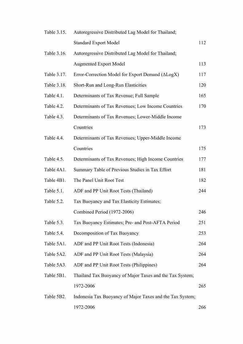
Table 3.15. Autoregressive Distributed Lag Model for Thailand;
Standard Export Model 112
Table 3.16. Autoregressive Distributed Lag Model for Thailand;
Augmented Export Model 113
Table 3.17. Error-Correction Model for Export Demand (ΔLogX) 117
Table 3.18. Short-Run and Long-Run Elasticities 120
Table 4.1. Determinants of Tax Revenue; Full Sample 165
Table 4.2. Determinants of Tax Revenues; Low Income Countries 170
Table 4.3. Determinants of Tax Revenues; Lower-Middle Income
Countries 173
Table 4.4. Determinants of Tax Revenues; Upper-Middle Income
Countries 175
Table 4.5. Determinants of Tax Revenues; High Income Countries 177
Table 4A1. Summary Table of Previous Studies in Tax Effort 181
Table 4B1. The Panel Unit Root Test 182
Table 5.1. ADF and PP Unit Root Tests (Thailand) 244
Table 5.2. Tax Buoyancy and Tax Elasticity Estimates;
Combined Period (1972-2006) 246
Table 5.3. Tax Buoyancy Estimates; Pre- and Post-AFTA Period 251
Table 5.4. Decomposition of Tax Buoyancy 253
Table 5A1. ADF and PP Unit Root Tests (Indonesia) 264
Table 5A2. ADF and PP Unit Root Tests (Malaysia) 264
Table 5A3. ADF and PP Unit Root Tests (Philippines) 264
Table 5B1. Thailand Tax Buoyancy of Major Taxes and the Tax System;
1972-2006 265
Table 5B2. Indonesia Tax Buoyancy of Major Taxes and the Tax System;
1972-2006 266

Table 5B3. Malaysia Tax Buoyancy of Major Taxes and the Tax System;
1972-2006 266
Table 5B4. Philippines Tax Buoyancy of Major Taxes and the Tax System;
1972-2006 266
Table 5B5. Thailand Tax Elasticity of Major Taxes and the Tax System;
1972-2006 267
Table 5B6. Indonesia Tax Elasticity of Major Taxes and the Tax System;
1972-2006 267
Table 5B7. Malaysia Tax Elasticity of Major Taxes and the Tax System;
1972-2006 268
Table 5B8. Philippines Tax Elasticity of Major Taxes and the Tax System;
1972-2006 268
Table 5B9. Thailand Tax Buoyancy of Major Taxes and the Tax System;
1972-1991 268
Table 5B10. Indonesia Tax Buoyancy of Major Taxes and the Tax System;
1972-1991 269
Table 5B11. Malaysia Tax Buoyancy of Major Taxes and the Tax System;
1972-1991 269
Table 5B12. Philippines Tax Buoyancy of Major Taxes and the Tax System;
1972-1991 269
Table 5B13. Thailand Tax Buoyancy of Major Taxes and the Tax System;
1992-2006 270
Table 5B14. Indonesia Tax Buoyancy of Major Taxes and the Tax System;
1992-2006 270
Table 5B15. Malaysia Tax Buoyancy of Major Taxes and the Tax System;
1992-2006 270

Table 5B16. Philippines Tax Buoyancy of Major Taxes and the Tax System;
1992-2006 271
Table 5C1. Thailand – Tax-to-Base; 1972-2006 273
Table 5C2. Thailand – Base-to-Income; 1972-2006 273
Table 5C3. Indonesia – Tax-to-Base; 1972-2006 273
Table 5C4. Indonesia – Base-to-Income; 1972-2006 273
Table 5C5. Malaysia – Tax-to-Base; 1972-2006 274
Table 5C6. Malaysia – Base-to-Income; 1972-2006 274
Table 5C7. Philippines – Tax-to-Base; 1972-2006 274
Table 5C8. Philippines – Base-to-Income; 1972-2006 274
Table 5C9. Thailand – Tax-to-Base; 1972-1991 275
Table 5C10. Thailand – Base-to-Income; 1972-1991 275
Table 5C11. Indonesia – Tax-to-Base; 1972-1991 275
Table 5C12. Indonesia – Base-to-Income; 1972-1991 275
Table 5C13. Malaysia – Tax-to-Base; 1972-1991 276
Table 5C14. Malaysia – Base-to-Income; 1972-1991 276
Table 5C15. Philippines – Tax-to-Base; 1972-1991 276
Table 5C16. Philippines – Base-to-Income; 1972-1991 276
Table 5C17. Thailand – Tax-to-Base; 1992-2006 277
Table 5C18. Thailand – Base-to-Income; 1992-2006 277
Table 5C19. Indonesia – Tax-to-Base; 1992-2006 277
Table 5C20. Indonesia – Base-to-Income; 1992-2006 277
Table 5C21. Malaysia – Tax-to-Base; 1992-2006 278
Table 5C22. Malaysia – Base-to-Income; 1992-2006 278
Table 5C23. Philippines – Tax-to-Base; 1992-2006 278
Table 5C24. Philippines – Base-to-Income; 1992-2006 278

Table 5D1. Cointegration test for variables used for computing
tax buoyancy; Combined period (1972-2006): Thailand 280
Table 5D2. Cointegration test for variables used for computing
tax buoyancy; Combined period (1972-2006): Indonesia 280
Table 5D3. Cointegration test for variables used for computing
tax buoyancy; Combined period (1972-2006): Malaysia 280
Table 5D4. Cointegration test for variables used for computing
tax buoyancy; Combined period (1972-2006): Philippines 281
Table 5D5. Cointegration test for variables used for computing
tax elasticity: Thailand 281
Table 5D6. Cointegration test for variables used for computing
tax elasticity: Indonesia 282
Table 5D7. Cointegration test for variables used for computing
tax elasticity: Malaysia 282
Table 5D8. Cointegration test for variables used for computing
tax elasticity: Philippines 282
Table 5D9. Cointegration test for variables used for computing
tax buoyancy; Pre- and Post-AFTA periods: Thailand 283
Table 5D10. Cointegration test for variables used for computing
tax buoyancy; Pre- and Post-AFTA periods: Indonesia 283
Table 5D11. Cointegration test for variables used for computing
tax buoyancy; Pre- and Post-AFTA periods: Malaysia 284
Table 5D12. Cointegration test for variables used for computing
tax buoyancy; Pre- and Post-AFTA periods: Philippines 284
Table 5D13. Cointegration test for variables used for the decomposition
of tax buoyancy; Combined period (1972-2006): Thailand 285

Table 5D14. Cointegration test for variables used for the decomposition
of tax buoyancy; Combined period (1972-2006): Indonesia 285
Table 5D15. Cointegration test for variables used for the decomposition
of tax buoyancy; Combined period (1972-2006): Malaysia 285
Table 5D16. Cointegration test for variables used for the decomposition
of tax buoyancy; Combined period (1972-2006): Philippines 285
Table 5D17. Cointegration test for variables used for the decomposition
of tax buoyancy; Pre-AFTA period (1972-1991): Thailand 286
Table 5D18. Cointegration test for variables used for the decomposition
of tax buoyancy; Pre-AFTA period (1972-1991): Indonesia 286
Table 5D19. Cointegration test for variables used for the decomposition
of tax buoyancy; Pre-AFTA period (1972-1991): Malaysia 286
Table 5D20. Cointegration test for variables used for the decomposition
of tax buoyancy; Pre-AFTA period (1972-1991): Philippines 287
Table 5D21. Cointegration test for variables used for the decomposition
of tax buoyancy; Post-AFTA period (1992-2006): Thailand 287
Table 5D22. Cointegration test for variables used for the decomposition
of tax buoyancy; Post-AFTA period (1992-2006): Indonesia 287
Table 5D23. Cointegration test for variables used for the decomposition
of tax buoyancy; Post-AFTA period (1992-2006): Malaysia 288
Table 5D24. Cointegration test for variables used for the decomposition
of tax buoyancy; Post-AFTA period (1992-2006): Philippines 288
Table 6.1. Average Tariff of Top 10 Items Under Tariff Restructuring
in Thailand, 2002 – 2005 307
Table 6.2. Nominal and Effective Rates of Protection
in Thailand 1908-2003 (percent) 308
Table 6.3. Thailand GDP by Sector, 2000 - 2008 (percent) 311

Table 6.4. Revenue from Tourism, 2000 – 2008 312
Table 6.5. Tax on Consumption and Tax Refund, 2000 – 2008 313

Chapter 1
INTRODUCTION
1

1.1. General Introduction and Motivation
Since World War II, most countries have experienced a rapid pace of the integration
of domestic economies into the international economy through the intensification of
the process of globalization. Globalization is a phenomenon which involves increases
in the flows of trade, capital, information and technology, as well as the mobility of
labour across borders. This period of rapidly increased globalization is associated with
a substantial expansion in international trade, world production, and consequently, a
rise in world economic welfare. In general, globalization encourages a free flow of
trade and investment across countries via the process of trade liberalization. Trade
liberalization is normally associated with the reduction, removal and elimination of
taxes on goods and services (including tariffs and import duties), and other trade
barriers such as quotas on imports, subsidies, and non-tariff barriers to trade. It also
includes the removal of trade-distorting policies, free access to market, free access to
market information, the reduction of monopoly or oligopoly power, free movement of
capital and labour between and within countries, and the creation of free trade zones.
Trade liberalization may also take many forms such as free trade zones, free trade
area, trade blocs, and free trade agreements at bilateral, multilateral, or regional
agreements.
The spread of trade liberalization over the world in the last decade has been driven by
its numerous benefits. The most outstanding advantage of free trade, which induces
most countries to walk toward free trade regime, is that open trade policies lead to a
better economic performance. In fact, the possible gains from trade have long been
pointed out by the early classical theorists; David Ricardo and Eli Heckscher. They
suggest that these gains result from specialization in production due to international
trade. If a country specializes according to its comparative advantage, the allocation
2

of domestic resource can be enhanced. This achievement improves the efficiency of
production because resources which have formerly been employed in the production
of other goods are now shifted to the production of the goods which a country
produces best. Consequently, the income and welfare of all trading partners will be
improved. Although an economy grows over time as a result of increases in its
productive resources and technology innovation, most of the economic literature
suggests that trade liberalization potentially improves the allocation of domestic
resources and consequently leads to an increase in economic welfare. According to
Dornbusch (1992), Salehezadeh and Henneberry (2002), and Dennis (2006), every
kind of import restrictions raises the price of import goods relative to export goods.
The removal of trade restrictions through the process of trade liberalization
encourages a shift of domestic resources from the production of import substitutes to
the production of export-oriented goods. Thus, the new allocation of resources due to
trade based on comparative advantage provides large benefits to domestic production
and generates growth in the medium to long term. On contrary, trade liberalization
may also have a negative effect on economic growth since it exposes a country to
volatility of output and terms of trade. Grossman and Helpman (1991) and Srinivasan
(2001) have developed endogenous growth models in the study of trade liberalization
and suggested that free trade may be growth-hindering since it leads to more volatility
in some specific sectors. Trade liberalization is also often followed by financial
liberalization with the later associates with more financial fragility. Through these
channels, trade liberalization is considered as a potential source of macroeconomic
volatility which is an important determinant of a wide variety of adverse outcomes
including fluctuation in GDP growth. There are many recent studies which suggest
important adverse impacts of trade liberalization, for example, Ramey and Ramey
3

(1995) point out that higher macroeconomic volatility tends to lead to lower growth;
Pallage and Robe (2003) and Barlevy (2004) suggest that if output and consumption
smoothing is an issue for the government to stabilize the domestic economy, output
and consumption volatility will finally lead to the reduction of economic welfare;
Gavin and Hausmann (1998) and Laursen and Mahajan (2005) indicate that trade
liberalization induces inequality and poverty in developing countries. These studies
are supported by Harrison (1996), Harrison and Hanson (1999), Rodríguez and
Rodrik (1999), which suggest that the positive association between trade liberalization
and economic growth found in many previous studies is flawed, particularly due to
the chosen measures of trade openness and model specification. They conclude that
those results are not robust and they fail to establish the relationship between more
open trade regimes and long-run economic growth. However, Greenaway, Morgan,
and Wright (1998) and Bolaky and Freund (2004) suggest that trade liberalization
may result in either an increase or a decrease in economic growth, depending on the
country’s characteristic and condition.
However, there are many examples which strongly support the argument that
openness to international trade brings more rapid growth to the country. According to
the World Bank (2002), almost half of developing countries which have lowered their
average tariffs by about 30 percentage points, are associated with an increase in trade
relative to income by over 80 percent in the post-1980 period, and experienced growth
of per capita income by 4 percent per annum in the 1980s, and 6 percent in the 1990s.
By contrast, the remaining developing countries, which have lowered average tariffs
by only 10 percentage points, are experienced very little or even no growth in GDP
per capita in the post-1980 period. From this evidence, many authors suggest that the
channel through which trade liberalization results in economic growth is by increasing
4

the volume of trade between countries.1 Since the empirical evidence suggests that
policies to promote trade openness, supported by sound domestic policies, leads to
faster growth, and, in line with the experience that the earlier strategy of attempting to
achieve growth through import substitution has been conclusively proved to have
failed, most developing countries have switched their trade policies from import
substitution to export promotion by implementing trade liberalization policy since
1980s.
Generally, there are three routes for trade to generate growth; the increase in domestic
demand, import substitution, and export promotion. An increase in domestic demand
is associated with the stimulation of expenditures inside the country, while import
substitution and export promotion are related to international trade effects. In general,
most developing and less developed countries have begun their economic
development by inducing an import substitution strategy in the first phase. Import
substitution is a strategy which reduces the country’s foreign dependency and
appreciates the domestic production by substituting the imported goods with the
locally produced goods. This strategy aims to protect domestic industries, i.e. infant
industries, until they are able to compete with the foreign industries. However, it
appears that the country that can benefit from an import substitution strategy is
generally rich and must have a large economy and huge internal market.
Unfortunately, most of the less developed and developing countries appear to have
smaller economies with lower per capita income. These countries are less likely to
succeed with an import substitution strategy. Therefore, in practice, the majority of
less developed and developing countries have shifted their policies from import
substitution in the first phase to serve for an export promotion strategy in the next
1 See Sengupta and Espana (1994) and Ramos (2001), for example.
5
phase, by hoping that an export promotion strategy will stimulate growth more
rapidly. On the other hand, an export promotion strategy, instead of promoting
industries which produce import substituted goods and protect infant industries,
particularly promotes the industries that have the potential for developing and
competing with foreign rivals in the world market. In order to gain an access to a
foreign market, liberalization policy is implemented to assist an export promotion
strategy. According to Edwards (1993), more liberalized economies have faster
growth of exports and in turn, this results in more rapidly growing country’s income.
Thus, over the past few decades, liberalizing the external trade regime has been one of
the central and most visible elements of many less developed and developing
countries to achieve accelerated exports, and consequently economic growth.
However, not all countries have benefited from the gains of trade liberalization. From
a trade perspective, while trade liberalization is generally associated with a substantial
increase in the volume of imports, there is nothing to guarantee that every country
participating in free trade will experience a considerable increase in the volume of
exports. Furthermore, if, after trade is liberalized, exports do not increase
proportionately as an increase in imports, the trade balance will be worsened further
and further. High imports without corresponding increases in exports leads to a trade
deficit and further results in a current account problem. On the fiscal side, trade
liberalization is likely to lead to a substantial decrease in international trade tax
revenue through the reduction of tariffs. The fiscal problem is more serious if a
country is highly dependent on international trade tax and if it places this tax as a
major source of government revenue. Usually, this fiscal problem is found in less
developed and developing countries. Thus, trade liberalization may in turn potentially
6

lead the country to a profound problem of deficits which includes both trade deficit
and fiscal deficit, at least in its transition period.
Generally, countries’ reliance on international trade tax is inversely related to their
income levels. This is because most of less developed and developing countries
usually lack administrative capacity which in turn reduces the efficiency of tax
collection. In addition, these countries also have large informal and subsistence
sectors which mean that a considerable amount of transactions cannot be taxed.
Furthermore, the influence of powerful lobbies creates a limitation for the tax
authorities to collect revenue in some sectors. Since domestic tax bases are limited,
the government has to meet its fiscal need by charging high rates on such an easy-to-
tax source as trade taxes and placing high dependence on international trade taxes.
With governments operating under a liberalization regime, revenue-declining
concerns are often considered as a serious issue for governments in implementing
trade and tax reform.
Although the revenue from an international trade tax has become less important over
the past few decades, it still continues to be a major source of government finance in
many less developed and developing countries. According to the WTO (2002),
international trade tax has generated on average 24.3 percent of total current revenues
over the last decade; for less developed and developing countries the share goes up to
36.2 and 28.7 percent, respectively. This compares to 1.3 percent for high-income
Organization for Economic Cooperation and Development (OECD) countries and 3.7
percent for developed countries. Thus, while the data show a decreasing trend
worldwide, less developed and developing countries are still highly dependent on this
tax source. As a consequence, even countries that are persuaded to enjoy substantial
economic growth and to reap other benefits from trade liberalization, most of less
7

developed and developing countries may fear of the very high cost of trade
liberalization in terms of the loss of tax revenue.
Certainly, domestic taxation is the first option for a government to manage with fiscal
problem rooted from trade liberalization since it is the most important instrument for
augmenting revenue, especially for less developed and developing countries.
Economists suggest that, in order to mitigate the loss of international trade tax
revenue, one strategy is to raise both domestic direct and indirect taxes, particularly
increasing revenue from goods and services tax, by implementing domestic tax
reform. By substituting revenue sources from international trade tax to broad-based
domestic taxes, economists believe that the negative impact of trade liberalization can
be offset or reduced. However, the suggestion that the fiscal problem can be
eliminated if trade liberalization is coordinated with domestic direct and indirect tax
may not be able to efficiently follow since trade liberalization may not only have a
directly negative impact on international trade tax, but it may possibly have an
indirectly adverse impact on various individual tax revenues. For example, trade
liberalization is always accompanied with other processes including privatization,
restructuration, and automation, which potentially cause tremendous job losses. These
processes may also link with cuts in wages and wage dumping. Consequently, the
process of trade liberalization may result in the contraction of the personal income tax
base, and thus the decline in personal income tax revenue. However, it is difficult to
draw any firm conclusions on the impact of trade liberalization on employment since
it is highly dependent on the growth effect of trade liberalization, country-specific
effect, and other contingent factors. Trade liberalization may also have an impact on
corporate income tax through changes in the exchange rate. Normally, exchange rate
depreciation occurs after trade is liberalized, while the price of imports is usually low
8

relative to price of domestic goods. This will possibly lead to a decline in the real
exchange rate, a rise in the relative price of imported inputs used by corporations in
production, and finally lower profitability of firms. However, in the currency
depreciation situation, exporters might benefit through stronger sales, but whether it
can be offset by higher input costs is still questioned. Thus, the impact of trade
liberalization on the corporate income tax base is still ambiguous. Trade liberalization
may be harmful to the tax on goods and services, mainly through changes in its tax
base. Generally, tariffs are applied to the import value. Then, excise tax is levied on
the base inclusive of tariffs. When imported goods enter into the domestic market,
such a goods and services tax as VAT is levied on the base inclusive of tariffs and
excise duties. Normally, trade liberalization is associated with the reduction or
elimination of tariffs. This possibly leads to a fall in the tax base since tariffs
constitute an element of the goods and services tax base. However, a high reduction of
tariffs may lead to a drastically increase in the volume of imports, offsetting the
decline in the value of imports. In addition, goods and services tax revenue may also
decline if there is a decrease of the output of import-substituted goods. However, in
the long term, if trade liberalization leads to economic growth, the growth of the
economy is likely to expand the consumption tax base, and consequently results in an
increase in the goods and services tax. Thus, again, the firm conclusion of how trade
liberalization affects the goods and services tax cannot be drawn.
Another strategy to mitigate the loss of international trade tax revenue is to strengthen
tax administration and collection and to improve the effectiveness of the tax system.
However, as discussed above that trade liberalization may have various adverse
impacts on many tax types, as a result, the performance of overall tax system would
be deteriorated. Until recently, many less developed and developing countries still
9

have experienced the difficulty in raising tax revenue to the level which is required to
promote the growth of their economies. A poor tax performance, in terms of raising
tax revenue, can mean either deficiency in the capability of tax administration, an
inadequate effort to collect or the deterioration of tax bases, or both. In order to
improve the performance of the overall tax system, domestic tax reform is a necessary
process. Tax reform is usually a basic component of trade liberalization. The key
objective of tax reform under the trade liberalization regime is to ensure that the tax
system is productive enough to mitigate the fiscal imbalance. In general, countries
which embark on the liberalization path also perform domestic tax reform at the same
time, in order to modernize their tax systems, with the hope that tax reform will
reduce compliance and collection costs, improve tax administration, and consequently
enhance revenue collection. Therefore, it is important to review tax revenue
performance as well as tax design and administration changes during the liberalization
period.
Thus, the following questions are addresses in this thesis:
1. What are the factors determining imports and exports? How does trade
liberalization affect the volume of imports and exports in both the short run
and the long run?
2. What is the impact of trade liberalization on domestic and international trade
taxes? How does the impact differ among countries with different level of
development?
3. How is trade liberalization associated with the enhancement of the
performance of the overall tax system? Which components of tax structure
have been the most responsive or rigid?
10

1.2.Various Issues Related to Trade Liberalization
1.2.1. Trade Liberalization and Structural Adjustment
During the 1980s and 1990s, there has been significant trade liberalization by
developing countries under the aegis of structural adjustment programs suggested by
the World Bank and the IMF. According to the original Washington Consensus, a
term attributed to Williamson (2003), the components of structural adjustment
reforms, in addition to trade liberalization, are;
1) Fiscal discipline; government budget deficits must be reduced.
2) Reorientation of public expenditures; public expenditures must be
reprioritized, especially to education, health care, and infrastructure
investment.
3) Tax reform; tax structure must be reformed by broadening the tax base and
adopting moderate marginal tax rates.
4) Financial market liberalization; lower interest rates must be set and subsidies
on interest rates must be eliminated. Financial markets must be deregulated.
5) Unified and competitive exchange rates; since international debt and trade
deficits are the major problems which lead to structural adjustment programs,
exchange rate devaluation is necessary because it solves the overvaluation of
exchange rates.
6) Openness to foreign direct investment; it is necessary to increase the rate of
the investment in developing countries and bring resources which would
otherwise be unavailable for economic growth.
11

7) Privatization; the ownership of a business, enterprise, agency, and public
service must be transferred from public sector to private sector in order to
reduce the role of inefficient and corrupt government.
8) Deregulation; any government rules and regulations that impede market entry
or restrict competition must be removed or simplified.
9) Secure property rights; property rights must be clearly established in legal
frameworks so that the incentives under structural adjustment programs could
be pursued.
Because structural adjustment programs have usually been imposed on developing
countries governments rather than on those of developed economies, and because they
imposed substantial hardship on populations, these programs have not always been
embraced nor pursued fully. Incomplete adoption of the Washington consensus has
led to some controversy concerning its effectiveness. Some critics have argued that
the failure of structural adjustment to work in many countries is not only due to too
little or too much reform, but also due to the reform is too soon for a country to
prepare, and also there are wrong sorts of reforms. Among critics with various
opinion, Rodrik (2006) pointed out a factual paradox; the fact that China and India
turn out to be successful in stimulating growth while their general economic policies
have remained opposite to the recommendations of the Washington consensus. And
since the evidence that the effects of the reform of macroeconomic policies, fiscal
policies, and trade openness on national growth rates is quite weak, Rodrik (2006)
suggested that those reforms are ineffective because the reform does not specifically
focus on the area which has the most binding constraints on economic growth. He
suggested that, after identifying the most binding constraints, appropriate policy
responses must be generated and institutional reform must be taken place. A
12

government is needed to ensure appropriate institutions are put in place. Institutions
are crucial to both the success of structural adjustment programs and to economic
development. Legal and regulatory frameworks must be established and new market
structures are needed.
Considering trade liberalization, the most common policy reform recommended to
developing countries, Rodrik (2006) indicated that trade liberalization must be
accompanied by complementary adjustment policies, particularly macroeconomic
reform, and must go along with a long list of conditions, in order to be effective and
to be ensured to enhance welfare. One of many conditions is that there must be no
adverse effects on the fiscal balance, or if there are, there must be alternative and
expedient ways of making up for the lost fiscal revenues. Although he believes that
trade policy is overemphasized, and that macroeconomic reform and institutional
innovations are far more important in fostering economic growth, he agrees that trade
liberalization accompanies development and that in long run an economy which fails
to integrate with international markets will grow more slowly.
1.2.2. Trade Liberalization, Economic Growth, and National Welfare
Under certain circumstances, a country’s overall welfare is in some sense improved
by freer trade, which should thus be viewed as desirable. In simplest terms, the
welfare gains from trade come from the fact that a country that moves from autarky to
free trade gets to trade at a price ratio different from the autarky price ratio. As a
result, this must make a country better off. This is the most basic form in which a
country enjoys welfare benefits in moving from autarky to free trade. Opening up to
trade offers an opportunity to trade at international prices rather than domestic prices.
This opportunity in itself offers a gain from exchange, as consumers can buy cheaper
13

imported goods and producers can export goods at higher foreign prices. Further,
there is a gain from specialization as the new prices established in free trade
encourage industries to reallocate production from goods that the closed economy was
producing at relatively high cost to goods that it was producing at relatively low cost.
Thus, the static gains from trade arise from shifting the mixed outputs toward goods
of comparative advantage, by holding fixed the economy’s technology and
endowments so its production possibility frontier (PPF) remains static, while
permitting consumers to take advantage of the new price. However, the fact that
technological change is endogenous means that a move from autarky to free trade has
additional dynamic welfare effects. The static analysis ignores many dynamic
consequences of trade liberalization. There are many authors suggesting that a
dynamic setting free trade is harmful to economic growth. For instances, Findlay
(1980) presented the use of a dynamic two-region model, each region producing a
distinctly different product. In order to embody interregional differences, he proposed
that the labour markets of each region have dissimilar structures. Specifically, the
North is assumed to manufacture the investment good using the services of all
available capital and labour. In contrast, labour is in perfectly elastic supply at a
constant real wage in the South, a primary consumption good producer. By assuming
these asymmetries between regions, he developed a vigorous formal analysis and
showed that trade is the engine of growth for the South. The power of the engine is
determined, however, by the natural growth rate of the North, and in this sense the
South does not have its own growth engine. Technological improvements also have
asymmetrical results. Hicks-neutral or Harrod-neutral shifts in the production function
of the North leave the terms of trade unchanged in the long run and increase its real
per-capita income. In the South, however, a Solow-neutral shift in the production
14

function leads to a proportional decline in the terms of trade and brings about a
decrease in its real per-capita income measured in terms of manufactured goods.
Another well-recognized dynamic analysis of welfare gains from freer trade is
Krugman (1981). In order to show that initial discrepancy in capital-labour ratios of
the two adjacent, competing regions will cumulate over time, and will inevitably lead
to the division into the capital-rich, industrial region and capital-poor, agricultural
region, he developed a two region model of uneven regional development and
examined the effect of international trade upon the world distribution of income when
there are external economies to physical capital accumulation in the manufacturing
sector. That is, more-industrialized countries cumulatively accumulate capital than
less-industrialized countries under the assumption of increasing return of technology.
In his model, there are two countries, North and South, which have the same amount
of labour force and produce two goods, a manufacturing good and agricultural
product. A single world price of manufacturing goods in terms of agricultural
products was assumed. In other word, a single world price of agricultural products
was set to unit. Manufacturing production was assumed as a function of capital input
and labour input, and its technology is increasing return, while agricultural products
were assumed to be produced by labour alone. In addition, labour forces were
assumed to consume agricultural goods alone, and their saving ratios are zero which
means unit labour cost to be one. Under these assumptions, he first investigated the
North-South relationship by assuming there is international trade but no international
capital movement. Because the profit rate of the manufacturing sector of the North is
higher than that of the South, capital accumulation in the North is faster than in the
South. If North-South relation starts where Northern capital stock is larger than
Southern capital stock, northern manufacture will grow faster and finally North will
15

become industrial region and South will be specialized in agriculture (or at least less-
industrial region). He then allowed international investment by assuming the
movement of capital between two regions. With capital mobility, there is a two-stage
pattern of development which trade is the engine of growth in North through
increasing exports of manufactures in the first stage and then exports of capital in the
second stage, suggesting the justification of imperialism. In conclusion, freer trade in
dynamic aspect might a country (which is initially a “rich” country) to grow faster
than others (which are mostly “poor” and underdeveloped country) and this is the
Krugman’s theory of uneven development.
The concern that freer trade possibly leads to unequal development was also proposed
by Matsuyama (1992). In general, sectors differ in the degree of increasing returns to
scale and in growth potential. When freer trade leads to specialization in sectors with
low growth potential, it may have detrimental effects. Similarly, trade liberalization
can lead to the agglomeration of industrial increasing returns to scale activities in few
countries and this may have an adverse effect in the remaining regions of the world.
Countries which have comparative disadvantage in industrial sectors, especially in
less developed and developing countries, have a higher risk to suffer from the
negative impact of trade liberalization and globalization. From this concept,
Matsuyama (1992) constructed a model of a two-sector economy, agriculture and
manufacturing, with endogenous growth to demonstrate that a country specializing in
agriculture may be worse off after trade than in autarky. The key assumption of the
model is that the industrial sector is the engine of growth because learning by doing.
He shows that a high agricultural productivity is beneficial in closed economy, as it
releases resources that can be employed in the industrial. However, it may be
detrimental for a small open economy, as it may induce specialization in agriculture.
16
For the closed economy case, higher agricultural productivity, which is assumed to be
exogenous, translate into higher growth by shifting labour to manufacturing.
However, for the small open economy case, the small open economy will grow faster
than the world economy if it has a comparative advantage in the productivity in
manufacturing and vice versa, because growth is proportional to the fraction of labour
employed in manufacturing. Freer trade expands the sector of comparative advantage
and then learning by doing amplifies the initial comparative advantage. So, an
economy with less productive agriculture allocates more labour to manufacturing and
will grow faster. Thus, in this case, there is a negative link between agricultural
productivity and growth.
1.2.3. Trade Liberalization and “Contractionary” Devaluation
Governments embark on trade liberalization program in the hope to gain long-term
benefits from competition and comparative advantage. However, whatever long-run
benefits might be anticipated, the issues of short- and medium-run adjustment costs
are usually raised by those who oppose free trade since the costs are considerably
high. One of the most interesting issues related to trade liberalization is the
contractionary devaluation. Typically, trade liberalization is accompanied by
devaluation. The major policy objective of devaluation is to generate a readjustment
in the relative price of tradable and nontradable goods and to improve the external
position of the country. However, a number of authors recently have questioned the
effectiveness of devaluation as a policy tool. There is an argument that even though
nominal devaluation may achieve their goals of generating a relative price
readjustment and improving trade balance, these goals may be achieved at a very high
cost. In particular, it has been pointed out that one of such costs is the decline in total
17
output generated by devaluation. This critique has finally considered as the
contractionary devaluation problem.
From an analytical point of view, devaluation has an influence on the economy
through a number of channels. According to the more traditional view, devaluation
will either have an expansionary effect on aggregate output, or the worst case will
leave aggregate output unaffected. On one hand, if there is unutilized capacity,
nominal devaluation will be expansionary and total aggregate output will finally
increase. On the other hand, if the economy is operating under full employment,
nominal devaluation will be translated into equiproportional increase in prices, with
the real exchange rate and aggregate output being unaffected. Contrary to the
traditional view, there are several theoretical reasons which explain why devaluation
can be contractionary and how it generates a decline in aggregate real activity,
including employment. For example, Krugman and Taylor (1978) provided a
framework following a simple Keynes-Kalecki model of an open economy to analyze
the potential short-run effects of nominal devaluation. The assumptions underlying
their model are; i) there are two distinct sectors, one produces the (non-tradable) home
goods for domestic markets while the other produces the export goods for
international markets. ii) The price of home goods is determined by a mark-up over
direct input costs, while that of the imported input is fixed in terms of international
currency. iii) The nominal wage rate is constant in terms of the domestic currency. iv)
In the short run, substitution responses of both exports and imports to price changes
are negligible. v) Interest rates are kept constant by action of the monetary authorities.
Following these underlying characteristics, Krugman and Taylor (1978) concluded
that devaluation can lead to short-run contraction through three channels. First, in
general, a country which devalues its currency is in deficit at the time. In the presence
18

of a trade deficit, the valuation effect of an exchange rate change will be greater on
imports than on exports because of the greater initial volume of the imports. As a
consequence, there is the greater valuation effect of devaluation on imports in the
presence of a trade deficit and when measured in terms of the domestic currency.
Second, devaluation can generate a redistribution of income from groups with a low
marginal propensity to save to groups with a high marginal propensity to save,
resulting in a decline in aggregate demand and output. Third, a redistribution of
revenues from the private sector to the government sector which reduces demand for
the home goods, given a fixed level of government spending. Thus, in conclusion,
trade liberalization, when accompanied by devaluation policy, is likely to have
undesirable effects on economy by shifting the income distribution against labour and
reducing output and employment.
1.2.4. Trade Liberalization and Poverty Reduction
Among the most important concerns as trade liberalizes and economy integrates with
the world economy is the link between economic globalization and poverty. In
general, global economic integration has complex effects on income, culture, society,
and environment. However, in the debate over globalization’s merits, its impact on
poverty is particularly important. If international trade and investment primarily
benefit the rich, many people will feel that restricting trade to protect jobs, culture, or
the environment is worth the costs. But if restricting trade imposes further hardship on
poor people in the developing countries, many of the same people will think
otherwise. In a recent paper, Dollar and Kraay (2000) provided empirical evidence in
support of a positive and significant relationship between changes in trade and
changes in inequality, reaching the conclusion that expansions in trade raised growth
as well as incomes of the poor. They investigated the link between the income of the
19

poor and overall income (per capita GDP at PPP in 1985 international dollars). The
analysis was based on a sample of 80 countries over four decades and the poor are
defined as the bottom one fifth of the income distribution. From their paper, it can be
concluded that; i) On average across countries and over time, growth is distribution
neutral. ii) any factor which increases the growth rate is good for the poor. iii) The
income of the poor rises one-for-one with overall growth and the effect of growth on
the income of the poor is no different in poor countries than in rich countries. iv) The
income of the poor do not fall more than proportionately during economic crises. v)
The poverty-growth relationship has not changed in recent years. vi) Openness to
foreign trade benefits the poor to the same extent that it benefits the whole economy.
vii) Good rule of law and fiscal discipline benefit the poor to the same extent that they
benefit the whole economy. viii) No evidence is found that formal democratic
institutions or public spending on health and education have systematic effects on the
income of the poor. ix) World Bank and IMF policy packages increase the growth rate
and therefore, these policy packages should be the core of poverty reduction
strategies.
On the other side, antiglobalization activists are convinced that economic integration
has been widening the gap between the rich and the poor. Globalization benefits the
rich but does very little for the poor, perhaps even making them lot harder. There is a
number of criticisms and argument about the result of the work of Dollar and Kraay
(2000) placed by many authors such as Weisbrot et al (2001), and Nye, Reddy, and
Watkins (2002). The main criticisms of Dollar and Kraay (2000) can be concluded as
follows; i) The policy conclusions inferred by Dollar and Kraay (2000) from their
regressions are not persuasive as in most cases the results are statistically
insignificant. ii) The paper has no theoretical underpinnings or foundations. That is,
20

presumed relationships are not derived from any theoretical models. This comes to the
question of why there should be a one-to-one relationship between increases in per
capita income and the income of the poor. iii) Instead of using time series data, the
study is based on cross-country data, although some countries have very small
observations. This tells us very little about how individual countries will develop over
time. Although cross-country studies may indicate average trends, individual country
experiences can differ quite significantly. In fact, the use of a cross country
regression, based on the variability of income between countries, to infer the likely
temporal variability as economies grow is a very strong assumption. iv) The work of
Dollar and Kraay (2000) did not give any insight of how the income of the poor
changes when there are significant changes in the size distribution of income. In
addition, the case that the income growth of every quantile is proportionate to the
overall growth of GDP is not likely to be true. v) The definition of poverty used by
Dollar and Kraay (2000) is open to question. Taking the bottom quantile of the
income distribution as an indication of the extent of poverty is inadequate because it is
neither a measure of absolute poverty, nor is it an appropriate measure of relative
poverty. It tells us nothing about the relationship between the average income of the
bottom 20 per cent of income recipients and the poverty line, and it cannot highlight
changes that may occur in income distribution within the bottom quantile. Even if
economic growth does benefit the poor on a one-to-one basis, the poor would still fall
behind the rest of the population in absolute terms. vi) There are critical of the
openness index used by the work of Dollar and Kraay (2000) and further argue that
the regressions show no direct relationship between openness and the income of the
poor. That is, if freer trade is good for poverty reduction, it must have an indirect
effect through growth rather than a direct effect on poverty per se. vii) The variables
21

in the regressions show little or nothing about the relationships between most of the
variables examined, except for the correlation between economic growth and the
income of the poor. However, correlation does not imply causation. Even if there is a
relationship between the variable on the left hand side of the equation and the
independent variables on the right hand side, it may run in both directions and the
postulated regression is then a set of relationships characterizing the interrelationships
among jointly determined variables.
In conclusion, although there is strong evidence that economic growth normally
reduces income poverty, freer trade-led-growth still has many controversies. Since
there is no firm conclusion that freer trade leads to faster economic growth, there are
many argument whether freer trade should really reduce poverty, even in the long run.
In addition, the available cross-country data provide no clear evidence that trade
liberalization reduces poverty, at least in the short run. Thus, trade liberalization in the
hope that it will help reduce poverty should be done with care. Countries which
embark on trade liberalization need to have well-functioning social safety nets in
order to ease the tension between implementing trade reforms and alleviating poverty.
They also need to prepare some government budgets for offsetting some adverse
effects which trade liberalization may potentially lead to.
1.2.5. Trade Liberalization and External Shocks
Theoretically, there is only little evidence to support the claim that openness to trade
is associated with greater volatility. Moreover, even if this were the case, the idea that
the political system would then optimally deliver more insurance in the form of bigger
government is doubtful. As a consequence, recently, there has been interest in
investigating the relationship between trade openness and the size of government.
22

Among a number of papers, Rodrik (1998) demonstrated that a positive correlation
between trade openness and the size of government exists for a broad sample
including both developed and developing countries. He presented evidence to support
the hypothesis that larger governments provide social insurance in more open
economies facing higher terms of trade risk. If openness is associated with greater
risk, it is expected that openness is related to greater public expenditure to provide
greater social insurance. Rodrik (1998) used cross-country data to investigate the
nature of the relationship between trade openness (measured by the ratio of imports
plus exports to GDP) and government size (measured by the ratio of government
consumption to GDP) and found that there is a strong positive causation from the
former to the latter. Challenging the view that regards market and government as
substitutes, Rodrik (1998) took this evidence to suggest that there may be a degree of
complementary between them. Particularly, he argued that the causal relationship
between openness to trade and government size can be explained by compensation
hypothesis – that is the increased volatility brought about by growing exposure to, and
dependence on developments in the rest of the world creates incentives for
governments to provide social insurance against internationally generated risk. Since
trade openness raises exposure to risk, this reflects an increase in consumption
volatility and uneven income distribution, which is then reduced by a larger
government size.
From the suggestion that trade liberalization brings with it the necessity for larger
government to mitigate the volatility and external shocks, the capacity to tax for the
government in order to meet higher expenditure is of concern, especially for the
government in less developed and developing countries. In fact, the influence of
government in an economy goes beyond its spending and tax collection. State
23

ownership of enterprises, price control, mandate, and restrictions on competition are
examples of government intervention that can have profound effect on an economy.
All of these raise concerns that trade liberalization may have led to fiscal difficulties
and even inefficiently large government.
1.3. Outline of the Thesis
This thesis consists of three main chapters, all devoted to investigate the various
impacts of trade liberalization on trade and tax performance. In order to address the
first question, an empirical analysis is presented in Chapter 3 and investigates whether
there exists a long-run relationship between trade and its major determinants. It also
examines the impact of trade liberalization on the volume of imports and exports. In
the analysis of trade liberalization and the formation of trade policy, one of the major
concerns of policy makers is the responsiveness of trade flow to change in income and
relative price. The impact of trade liberalization policy is highly dependent on the size
of income, import price, and export price elasticities. As far as the analysis of import
price, export price, and income elasticities is concerned, the empirical investigation of
import and export demand functions is one of the most interesting research areas of
international economics. International economists have dedicated a substantial
amount of effort to the estimation of import and export demand functions, both at the
aggregate and disaggregated levels. Estimated elasticities are very important for
policy makers since they represent a crucial link between trade policies and changes
in trade flow, the degree to which trade policies affect the balance of payments and a
country’s economic performance.
Therefore, Chapter 3 highlights one of the key issues which currently has a wide
academic and political controversy by focusing on the question whether trade
24

liberalization really brings about an increase in international trade. This chapter seeks
to estimate the likely impact of trade liberalization policies on the volume of imports
and exports using aggregated import and export demand functions in Thailand for the
period 1960 to 2007. Thailand is one of the developing countries that grew rapidly
during the past two decades. Thailand, like many other developing countries, has
switched from a closed economy to a more open economy by inducing free trade
policies in the hope that trade liberalization will bring an improvement in its overall
economic performance and address balance of payments difficulties. Thailand has
formally introduced trade liberalization policy with its membership of AFTA in 1992
and the WTO in 1995, though its tariffs have been gradually reduced over time. By
opening the country, Thailand primarily hopes to achieve better export performance
and hence alleviate the ongoing trade deficit problem. Although, there is still a
concern that trade liberalization is generally found to be positively associated with the
volume of imports, while it may not lead to an increase in the volume of exports in the
same proportion, it is found that, for Thailand, the volume of exports has exceeded the
volume of imports for almost all years in the post-liberalization period.
Thus, in Chapter 3, we put an effort to assess empirically the major determinants of
import and export demand functions in Thailand using the cointegration technique to
estimate the long-run relationship and error-correction mechanism to examine the
dynamic behaviour. We, then, estimate the income and price elasticities from both
import and export demand functions by using an Autoregressive Distributed Lagged
(ARDL) model. We also compare these estimates with the estimates obtained using
cointegration techniques and an ECM. Finally, we analyze the impact of trade
liberalization on the volume of imports and exports in both the short run and long run.
25

When compared with the studies of free trade related growth, employment, or trade
creation and diversion, there have been a relatively small number of both theoretical
and empirical studies on the revenue impact of trade liberalization. This is an equally
important area of inquiry, because if trade liberalization leads to a reduction in tax
revenues, this can have serious implications for fiscal reform of countries that have a
budget constraint. Hence, after we investigate the impact of trade liberalization on
trade performance, we turn our focus to its impact on tax revenues, in order to shed
light on a controversy whether trade liberalization is a potential source of fiscal
instability, especially for countries which have high dependency on trade tax for their
public revenue. Although some authors suggest that trade liberalization could proceed
while adverse consequences can be avoided by coordinating liberalization with
potential government budget spending, sound macroeconomic policies, and effective
measures on the revenue; including raising domestic direct and indirect taxes,
widening and developing new tax bases, improving effectiveness of public spending,
raising public saving, and strengthening tax collection and administration, many
countries find that it is very difficult in practice to prevent the adverse effects on the
fiscal revenues.2 The problem is due to various restrictions such as the level of
development, the political instability, the constrained institutional capacities, and the
limitation of country’s geography.
Therefore, Chapter 4 is devoted to examine the effect on both international trade tax
and domestic taxes after trade is liberalized. As discussed above, although trade
liberalization is usually associated with the reduction of trade restrictions including
tariffs, and hence tends to lower international trade tax revenue, the relationship
between trade liberalization and other domestic tax revenues is still ambiguous, or
2 See Glenday (2002) and Keen and Ligthart (2004), for example.
26

even the impact on trade tax revenue itself is an empirical matter. In addition, tax
reform, in practice, is a very difficult task for many less developed and developing
countries to pursue. If trade liberalization is found to have a negative impact on
domestic tax revenues, domestic tax reform by using those instruments may be
inapplicable. This raises the further question of whether these countries should
implement the reform in the same way as it did in developed countries.
As stated earlier, the impact of trade liberalization on tax revenues may vary
depending on the level of development. Chapter 4 uses panel data of 134 countries
over 24 years covering the period 1980-2003 and divides countries into four groups;
low income, lower-middle income, upper-middle income, and high income countries.
However, the study concentrates on the impact of trade liberalization on tax revenues
of low and middle income countries since the sufferings from the loss of tax revenues,
if exist, are much higher for countries that have constrained government’s income
sources. Chapter 4 employs the traditional and extended tax effort model, using a
fixed-effects approach, with a two-way estimate, incorporating time and individual
country effects in order to obtain reliable results.
The impact of trade liberalization on tax revenue is investigated in more detail in
terms of the performance of the overall tax system. Domestic tax reform, which
usually is implemented at the same time as trade is liberalized, is an important
instrument for raising tax yield. In general, the productivity of the overall tax system
should be improved after the tax reform takes place. However, as mentioned earlier,
the effect of trade liberalization on the overall tax system is ambiguity. Trade
liberalization may either improve or deteriorate tax bases, depending on many
different factors. On one hand, fiscal revenue can be improved if trade liberalization is
accompanied by such supportive situations as a large expansion in international trade
27

volume, economic growth, employment, a rise in income level, and devaluation of
exchange rate. On the other hand, fiscal revenue can be deteriorated if trade
liberalization is associated with a shrink in trade volume, job losses, and deterioration
in corporate profit. Although it is difficult to determine accurately the direction of
change in overall tax revenue as a result of trade liberalization, changes in tax revenue
can be measured by applying the concept of tax buoyancy and tax elasticity since tax
revenue depends crucially on revenue productivity and tax structure (Suliman, 2005).
Growth in tax revenues may occur through automatic responses of the tax yield
through changes in national income and/or through the imposition of new taxes,
revision of the rate-structure of existing taxes, expansion of the tax bases, tax
amnesties, and tougher compliance and enforcement measures. Changes in tax yield
resulting from the modification of tax parameters (i.e., rates, base) are called
“discretionary changes” which stem from legislative action. Generally, tax buoyancy
and tax elasticity are the measures used to evaluate the ability of country’s tax system
to mobilize its revenue (Asher, 1989). Tax buoyancy measures the change in the
overall tax yield from changes in GDP whereas tax elasticity measures the change in
tax yield resulting from variations in national income with tax parameters held
constant (i.e., discretionary changes being removed). In Chapter 5, a measure of
revenue productivity of the tax system is used to determine whether the
responsiveness of tax revenues is high or low in Thailand relative to the other three
founding countries of the ASEAN Free Trade Area (including Indonesia, Malaysia,
and Philippines). By using the buoyancy and elasticity framework, Chapter 5 applies
the concept of tax buoyancy and elasticity to evaluate the implications of the process
of trade liberalization on revenue mobilization. The main objective of Chapter 5 is to
estimate tax buoyancy and tax elasticity of the Thailand tax system, compared to
28

those of its three neighbour countries. The evaluation is done to measure the response
of the tax system to trade liberalization by AFTA in 1992. By estimating tax
buoyancy and tax elasticity, this chapter addresses the question of whether Thailand’s
major trade liberalization by becoming AFTA members results in the enhancement of
the flexibility of the tax system. In addition, Chapter 5 decomposes tax buoyancy to
obtain the buoyancy of tax revenue with respect to its tax base and the buoyancy of
tax base with respect to income. The decomposition of tax buoyancy is beneficial
since it gives us capability of identifying factors which are responsible for rapid or
lagged revenue growth.
Finally, Chapter 6 reports the main findings, and draws policy implications. Possible
extensions for future research are also presented.
29

Chapter 2
A SURVEY OF THE THEORY OF TRADE
LIBERALIZATION
30

2.1. Introduction
When developing countries have reduced tariffs on tradable goods to improve the
allocation of their productive resources, these tariff cuts almost always lead to a loss
of government revenue. In most developed economies where their domestic tax bases
are well developed, the revenue loss can easily be offset by raising tax on
consumption. However, in most less developed and developing countries where the
international trade tax is the major source of tax revenue and the domestic tax bases
are not well developed, how to make up the shortfall in trade tax revenue, if there is
any, through other compensatory domestic taxes is still a major concern. With such a
heavy dependence on international trade tax as a major source of revenue, a key
concern for these countries is how to recover, from other tax sources, the revenue loss
that trade liberalization potentially entails.
In addition to widening the tax base and improving tax administration, a country
which undertakes a reduction in a tariff rate usually seek alternative domestic taxes to
substitute for the lost trade tax revenue. There are generally two strategies to offset
the revenue shortfall following a reduction in the tariff rate. The first is the strategy
using a domestic indirect tax, more specifically, a consumption tax. This strategy is
widely supported since using a broad-based consumption tax for revenue
compensation seems to be the most applicable approach in practice. The other
strategy is to use a domestic direct tax, more specifically a profit tax, to offset the
revenue shortfall. The rationale to use a profit tax as compensation is that the
producers are those who reap the profit from tariff reduction by reducing the price at a
very small proportion of tariff reduction to consumers. Therefore, producers are the
group who should receive this tax burden and a profit tax should be applied as a
compensatory measure.
31

This chapter provides theoretical underpinnings for the strategies to offset the revenue
shortfall from the loss of a tariff revenue due to tariff cut in order to provide a bird’s
eye view of the major theoretical contributions to the revenue implication of trade
liberalization. Section 2 is devoted to the strategy to offset the revenue shortfall as a
result of tariff reduction by using a broad-based consumption tax. Section 3 examines
the strategy to compensate the revenue shortfall by using a profit tax, a relative
narrow-based direct tax. The conclusion is contained in Section 4 of this chapter.
2.2. The Strategy to Offset Revenue Shortfall from The loss of Foreign Trade
Tax by Using Domestic Indirect Tax
Conventional models of trade liberalization typically assume that a fall in tariff
revenue in the post-liberalization period is offset by increasing consumption tax. Keen
and Ligthart (1999, 2004) suggest that, although the issue of trade tax revenue
reduction in many less developed and developing countries is very acute because tax
on international trade is their large source of revenue and their tax administration
capability is generally poor, there is still room for enhancing revenue in the period of
tariff reduction by coordinating a cut of tariff with a point-for-point increase in
domestic consumption taxes. With some rigorous conditions, this strategy ensures that
countries liberalizing their trade will end up with increases in both tax revenues and
welfare.
The following gives a brief summary of the model. The model considers a small open
economy and comprises three sectors; a representative household, a perfectly
competitive production sector, and a government. There are T tradable commodities.
World prices are denoted by . Taxes include tariffs p ( )τ and consumption taxes .
Thus producer prices are
( )t
p τ+ and consumer prices (q are ) p tτ+ + .
32

The expenditure function of the representative household is defined as
, where q is consumer prices and u is utility. ( , ) ; 0q qE q u E >
0The revenue function of the representative firm is defined as ( ) ; p pR p Rτ+ > ,
where p τ+ is producer prices.
It is assumed that public revenue from tariffs and consumption taxes ( ) will be
returned to consumers in the form of a lump-sum transfer. Thus, the income-
expenditure identity can be represented as:
G
Market Clearing Condition : ( , ) = ( ) + E q u R p Gτ+ (2.1)
Where = ( , ) + ( , ) ( )q q pG t E q u E q u R pτ τ⎡ ⎤⋅ ⋅ − +⎣ ⎦ (2.2)
The revenue from consumption taxation is denoted by the first term of equation (2.2),
while the revenue from tariffs is denoted by the second term of equation (2.2).
Consider a simultaneous tax reform by reducing tariffs by = 0n oτ τ τΔ − < (where nτ
and oτ r resent the “new” and “old” tariffs, respectively) and increasing consumption
taxes by an exactly offsetting amount = nt t
ep
0otΔ − > , (that is tτ−Δ = is
simultaneous reform results in the change of producer prices and so the domestic
production (as a reflection of tariff reduction), while consumer prices are entirely
unaffected (as a reflection of a point-for-point increase in consumption taxes). Tarff
reduction will result in an improvement in production efficiency and the
rearrangement of domestic production will consequently induces increases in the
value of output at world price. Since the value of output at world price increases,
welfare increases. Consider an increase in tax revenue. Initially, the government
collects revenue from a narrow-based tariff on imported commodities. The use of the
Δ ). Th
33

consumption tax will expand the tax base in which tax will be collected not only on
imported goods, but also on import substitutes produced domestically. As a
consequence, a coordinated tariff reduction with a point-for-point increase in
consumption taxes which maintain consumer prices unchanged will lead to an
increase in both government revenue and welfare.
Alternatively, this can be shown by using a simple diagrammatic interpretation as
presented in Figure 2.1.
Figure 2.1: Partial Equilibrium of Coordinated Tax-tariff Reform
For simplicity, we suppose that there are initially no consumption taxes. The only tax
that is collected by the government is the tariff and is set at 0τ . Initially, consumption
is at point t (line zt), domestic production is at point u (line zu), the amount of imports
is ut, and the public revenue is the area tuvw. After implemented a coordinated tax-
tariff reform by replacing the tariff 0( )τ with a consumption tax at exactly the
same rate
1( )t
0 1( )tτ = , the consumption still remains at point t but the domestic
production drops to point x (line yx), while the amount of imports increase from ut to
S
0 1p p tτ+ = +
y x
z tu
vw
D
p
34

xv. The initial (domestic) producer surplus (uxyz) disappears. However, public
revenue rises from tuvw to tvyz, with the additional revenue uwyz exceeding the
reduction in initial producer surplus (uxyz) by the amount of the improvement in
production efficiency (uwx). Thus, in summary, a reduction in tariffs accompanied by
an increase in consumption taxes that leaves consumer prices unchanged obviously
increases both tax revenue and welfare.
The main importance of this model is that it makes a first attempt to offer a formal
theory of policy reform to offset the loss of revenue caused by the tariff reduction.
While the advantage of this model is its ease of use, the assumption underlying the
model that it is base on perfect competition may be far from the real economy. In
addition, the result cannot be extended to deal with the reduction of tariffs on
intermediate goods used to produce tradable goods since it is not possible to offset a
tariff reduction by increasing consumption tax without affecting consumer price.
Following Keen and Ligthart (1999, 2004), many other economists have developed a
variety of models by changing the assumption from perfect completion to imperfect
competition in order to get closer to the real economy. Some models concentrate on
tariff reduction on intermediate inputs since these goods tend to be a major import in
most of less developed and developing countries. Other strategies besides using
consumption taxes to offset the loss of revenue are also proposed. In the following
section, we discuss a theoretical model in terms of imperfect competition and using
domestic direct tax to mitigate revenue loss from tariff reduction.
35

2.3. The Strategy to Offset Revenue Shortfall from The loss of Foreign Trade
Tax by Using Domestic Direct Tax
While Keen and Ligthart (1999, 2004) focus their study on offsetting the loss of tariff
revenue by using broad-based consumption taxes, other studies propose a strategy to
offset this loss by using a relatively narrow-based but less distorted profit tax.
Mujumdar (2004) gives two rational suggestions why the government should rely
more on a tax on firm profits instead of a commodity tax in order to achieve the offset
objective. First, many industries in most of less developed and developing countries
tend to have a very high oligopolistic power. Suppose that countries liberalize their
trade and if the price elasticity of demand is very low, which is likely to be, especially
in the case of the short run. Instead of reducing the price at the same proportion of
tariff reduction, producers may pass on only a small percentage of tariff reduction to
consumers by lowering the price by a very little amount and they may reap a
“windfall” profits of this tariff reduction. Therefore, it is reasonable for government to
collect tax revenue from such profits. Second, since it is generally perceived that
firms may make substantial profits from tariff reduction, there may be a very high
resistance from consumer groups if the government chooses to recover the revenue
shortfall by placing a higher consumption taxes and this possibly causes further
political problems. In fact, when the tariff rate of the intermediate input is reduced,
this will reduce tariff revenue on one hand, and will increase the firm’s profit by
reducing the cost of production of the final goods on the other hand. The higher
profits, together with the higher profit tax rate, will increase the profit tax revenue.
This revenue could be used to offset the shortfall generated by tariff reduction.
36

Tariff Reduction on an Intermediate Input under Imperfect Competition
Mujumdar (2004) suggests that though intermediate inputs constitute a large share in
world trade and thus deserves special treatment, very little effort has been made to
develop a tariff-tax reform strategies for this class of goods. In addition, he argues that
the model proposed earlier by Keen and Ligthart (1999) can be devised only under the
condition of a perfectly competitive production sector and hence cannot be extended
to cover an imperfectly competitive case. Thus Mujumdar (2004) considers the
question of whether government can make up a shortfall in revenue if it reduces a
tariff on an intermediate input under imperfect competition, while the make up by
using profit tax must ensure that both consumers and producers must be better off in
the post-liberalization period. The assumptions underlying the model are that an
industry comprises identical firms, importing the same intermediate input, so they
all have the same cost function. Each firm assembles all inputs to make a final
tradable product and sells its entire output in the domestic market.
N
Let denote the import price of the intermediate input. The model adopts the small
and open economy assumption by further assuming that all firms are price takers with
respect to the import price and changes in total quantity demanded of
intermediate inputs do not affect the import price ( . The (ad valorem) tariff
collected by the government is applied to the intermediate input at the rate t . The cost
of assembling intermediate input to produce each unit of output is assumed to be
identical across firms and is equal to c .
wP
( )wP
)wP
Let denote the output of firm i here iq 1, 2,...,i N= . Thus, the total cost function of
firm can be represented as: i
37

(1 )wiC P t c iq⎡ ⎤= ⋅ + + ⋅⎣ ⎦ (2.3)
The aggregate demand for the industry’s product can be shown as the inverse demand
function of firms’ output:
P a bQ= − (2.4)
where is the market price, and P1
N
ii
Q=
= q∑ , is the total industry output. It is also
assumed that purchasing the product from the domestic market is cheaper than
importing it.
Later, the firm profits will be taxed at the rate T (where 0 T 1≤ < ). Since the price of
output is equal to throughout the market, all firms are assumed to compete in
quantities.
P
The objective of any firm i is to maximize its after-tax profit and it can be shown by
maximizing firm’s profit, that is;
{ }Max (1 ) (1 )wi iT Pq P t c q⎡ ⎤∏ = − − + +⎣ ⎦ i
The model assumes that the firms compete like Cournot oligopolists in the product
market. Thus, for Cournot competition with many firms, the equilibrium output level
of each individual firm is:
(1 )( 1)
wci
a c P tqN b
− − +=
+ (2.5)
and thus the total equilibrium industry output is:
(1 )1
wc c
iN a c P tQ Nq
N b⎡ ⎤− − +⎛ ⎞= = ⎜ ⎟ ⎢ ⎥+⎝ ⎠ ⎣ ⎦
(2.6)
38
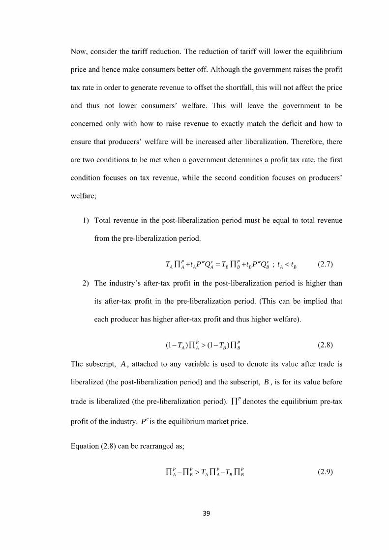
Now, consider the tariff reduction. The reduction of tariff will lower the equilibrium
price and hence make consumers better off. Although the government raises the profit
tax rate in order to generate revenue to offset the shortfall, this will not affect the price
and thus not lower consumers’ welfare. This will leave the government to be
concerned only with how to raise revenue to exactly match the deficit and how to
ensure that producers’ welfare will be increased after liberalization. Therefore, there
are two conditions to be met when a government determines a profit tax rate, the first
condition focuses on tax revenue, while the second condition focuses on producers’
welfare;
1) in the post-liberalization period must be equal to total revenue
from the pre-liberalization period.
Total revenue
P w c P w cA A A A B B B BT t P Q T t P∏ + = ∏ + Q B
The industry’
; (2.7) At t<
2) s after-tax profit in the post-liberalization period is higher than
its after-tax profit in the pre-liberalization period. (This can be implied that
each producer has higher after-tax profit and thus higher welfare).
(1 ) (1 )P PA A BT T B− ∏ > − ∏ (2.8)
he subscript,T , attached to any variable is used to denote its value after trade is A
liberalized (the post-liberalization period) and the subscript, B , is for its value before
trade is liberalized (the pre-liberalization period). P∏ denotes the equilibrium pre-tax
profit of the industry. cP is the equilibrium market price.
Equation (2.8) can be rearranged as;
PP P PA B A A BT T B∏ −∏ > ∏ − ∏ (2.9)
39

From equation (2.7), P P W c W cA A B B B B AT T t P Q t P∏ − ∏ = − AQ . Substitute this into the right-
hand-side (R.H.S.) of equation (2.9) and we have;
P P W c W cA B B B At P Q t P Q∏ −∏ > − A (2.10)
The tariff reduction reduces tariff revenue if;
(2.11) (1 )wB Aa c P t t> + + +
It is assumed that the condition stated in equation (2.11) holds. If equation (2.11) is
satisfied, it ensures that firm i will produce in the market.
The expression for PA∏ and in equation (2.10) can be re-written as; P
B∏
(1 ) (1 )c w c c w c W c W cA A A B B B B B AP c P t Q P c P t Q t P Q t P Q⎡ ⎤ ⎡ ⎤− − + − − − + > −⎣ ⎦ ⎣ ⎦ A (2.12)
Re-arranging terms in equation (2.12) and we have;
c w c c w cA A BP c P Q P c P Q⎡ ⎤ ⎡− − > − −⎣ ⎦ ⎣ B⎤⎦
w
(2.13)
Since the terms and c wAP c P⎡ ⎤− −⎣ ⎦
cBP c P⎡ ⎤− −⎣ ⎦ are both positive, we can rewrite the
equation as;
c cA Bc cB A
Q P c PQ P c P
− −>
− −
w
w (2.14)
Substituting cAQ and and simplifying equation (2.14), we have; c
BQ
(1 )(1 )
w wA
w wB A
a c P t a c P NP ta c P t a c P NP t− − + − − +
>− − + − − +
wB
w (2.15)
Since the numerator and the denominator on each side of equation (2.15) are positive,
we can re-arrange them to get;
[ ] [ ] [ ] [ ]( 1)( ) 1 ( 1)( ) 1w wA A A B Bt N a c P t N Nt t N a c P t N Nt− − + − − > − − + − − B (2.16)
40

If and the tariff is lowered but not eliminated, equation (2.15) gives us that
, which is true. If
1N =
A Bt t< 1N = and now the tariff is eliminated ( , instead of
reduced, equation (2.16) gives us that , which is also true. This can be
implied that when the industry is a monopoly, the government can determine a profit
tax rate in order to make up for revenue shortfall and make producers still better
off.
0)At =
20 (wBP t> − )
( )AT
Now, consider when and tariff is eliminated 1N > ( 0)At = . The left-hand-side
(L.H.S) of equation (2.16) turns out to be equal to zero, while the first term on the
R.H.S of equation (2.16) is positive but the second term is negative. Thus the net
value of the R.H.S cannot be determined and we cannot say that the L.H.S > the
R.H.S. We also cannot assert that the L.H.S > the R.H.S when and the tariff is
only reduced, but not eliminated. Thus, this implies that when there is more than one
firm in the industry, the government may not be able to determine a profit tax rate
in order to make up for revenue shortfall and make producers still better off.
1N >
( )AT
Therefore, from the model, Mujumdar (2004) concludes that only when the industry is
a monopoly can it be certain that raising the profit tax alone will generate enough
revenue to make up for the shortfall following a tariff reduction. This strategy can
also ensure that consumers and producers are better off in the post-liberalization
period as a result of an increase in welfare. However, the larger number of firms in the
industry lowers the probability that raising the profit tax alone is able to achieve the
purpose of the revenue offset and increasing welfare. This, consequently, leads the
government to use the more distortionary form of taxation, such as the consumption
tax, in order to meet the shortfall of tax revenue.
41

Tariff Reduction under the Condition of Product Differentiation
Haque and Mukherjee (2004) argue that the results proposed by Mujumdar (2004),
which indicate that only if the industry is a monopoly can we be certain that the
government could use the profit tax to make up any shortfall in tariff revenue and also
make both consumers and producers better off, are not robust when the products are
differentiated. When product differentiation is taken into the analysis, their model
shows that there always exists a degree of product differentiation such that the
government can achieve these objectives for any finite number of firms in the
industry. Thus, their results are more supportive for the government to reduce import
tariffs than those of Mujumdar (2004).
Following Mujumdar’s (2004) model, Haque and Mukherjee (2004) make
assumptions very similar to those used in Mujumdar’s (2002) work. The model
assumes a small open economy with an industry with symmetric firms so that the
input price remains constant irrespective of the imports by the firms. The assumption
of symmetric firms means that all firms have the same cost function and import a
certain key input. It is also assumed that one unit of output requires one unit of input
and the assembling cost of each unit is identical across firms. Unlike Mujumdar’s
(2004) model, they assume zero cost of assembly for simplicity since this does not
affect the qualitative results. They also assume no any other costs of production. For
each unit of import input, the ad valorem tariff t is imposed so the total cost of the
firm is;
N
thi
(2.17) (1 )wiC P t q= + i
The model assumes that the firm faces the inverse demand function as; thi
42

1
1
N
i ij
P a q qθ−
=
= − − j∑ (2.18)
where and . 1, 2,...,i N= i j≠ θ denotes the degree of product differentiation and
ranges from 0 to 1. The value of 0θ = implies isolated goods, while 1θ = implies
homogeneous products which corresponds to Mujumdar (2004).
The objective of the firm is to maximize profit which can be expressed as; thi
{ }Max (1 ) (1 )wi i iT Pq P t q⎡ ⎤∏ = − − +⎣ ⎦ i
The equilibrium output of the firm, thi 1, 2,...,i N= is:
(1 )2 ( 1)
wci
a P tqNθ
− +=
+ − (2.19)
and thus the total equilibrium industry output is:
(1 )
2 ( 1)
wc c
i
N a P tQ Nq
Nθ
⎡ ⎤− +⎣ ⎦= =+ −
(2.20)
and the equilibrium price charged by the firm is: thi
[ ]1 ( 1) (12 ( 1)
wc
i
a N PP
Nθ
θ)t+ + − +
=+ −
(2.21)
Consider when a tariff is reduced, equations (2.19) and (2.21) obviously show that
output of each firm has been increased while the price has been decreased, and thus
make the consumers better off. Again, the government has two objectives left to be
achieved; the revenue and producers’ welfare objectives.
In order for the government to be able to determine the profit tax in a way to make up
the shortfall in revenue, the increase in the industry’s pre-tax profit must be greater
than the shortfall in tariff revenue. Referring to equation (2.12), the only difference in
43

the following equation is that it assumes no cost of assembly. Thus, this case can be
written as;
(1 ) (1 )c w c c w c W c W cA A A B B B B B A AP P t Q P P t Q t P Q t P Q⎡ ⎤ ⎡ ⎤− + − − + > −⎣ ⎦ ⎣ ⎦ (2.22)
and equation (2.14) can be re-written as;
c cA Bc cB A
Q P PQ P P
−>
−
w
w (2.23)
Substituting cAQ , and c
BQ cAP , by using equations (2.20) and (2.21) and simplifying
equation (2.23), then we have;
cBP
(1 ) (1 ( 1))(1 ) (1 ( 1))
w wA
w wB A
a P t a P N P ta P t a P N P t
θθ
− + − + + −>
− + − + + −
wB
w (2.24)
and then we can re-arrange equation (2.24) to get;
( ) ( )( )( ) ( )( )
( 1) 1 1 1 ( 1)
1 1 1
wA A A
wB B
a N t P t N N t a N t
P t N N t
θ θ θ θ
θ θ
⎡ ⎤− − − + + − > −⎣ ⎦⎡ ⎤− − + + −⎣ ⎦
B (2.25)
or
*( )( 1) (1 )
wA B
wA B
P t tN a P t t
θ θ+< ≡
⎡ ⎤− − + +⎣ ⎦ (2.26)
From equation (2.26), since for any finite number of firms (as from equation
(2.11), ), the government can always find a profit tax to
achieve the revenue-welfare objective when the products are sufficiently
differentiated. This implies that for any given finite number of firms, there always
exists a degree of product differentiation such that the government can achieve this
goal. This result is in contrast to that of Mujumdar (2004). Haque and Mukherjee
(2004) suggest that because outputs and profits are continuous with respect to the
* 0θ >
0>(1 )wB Aa c P t t− + + +
44

degree of product differentiation, each firm becomes a near monopolist for its
products when the products are sufficiently differentiated. Therefore, the government
can use higher profit tax revenue to offset the shortfall of tariff revenue when the
degree of product differentiation is sufficiently high. However, if the products are not
very much differentiated, this will generate higher competition between the producers
as products become more substitutes. The higher competition between the final goods
producers, after the tariff rate is reduced, will not significantly increase their profits
and thus profit tax revenue may not be high enough to compensate the loss of tariff
revenue.
Equation (2.26) also presents the negative relationship between and N *θ . As the
number of firms increase, the competition between the final goods producers
increases.
( )N
*θ has been reduced, meaning that the product differentiation may not be
high enough to increase profits significantly, and hence the likelihood that the
government can use a profit tax to cover the loss of tariff revenue has been decreased.
Tariff Reduction under the Condition of Free Entry with a Certain Entry Cost
Haque and Mukherjee (2005) extend the analysis from their previous study by
examining whether the market under free entry with a certain entry cost can recover
the revenue loss as a result of tariff reduction on an intermediate input. Although the
analysis is on the intermediate goods in an imperfectly competitive product market so
the firms have significant market power, they allow for free entry with a certain entry
cost and find different revenue implications depending on the cost of entry. From their
findings, they suggest that, in the long run, a sufficiently large entry cost will generate
higher tariff revenue and profit tax revenue due to the entry of new firms into the
industry, and hence the market itself will compensate for any shortfall in revenue as a
45
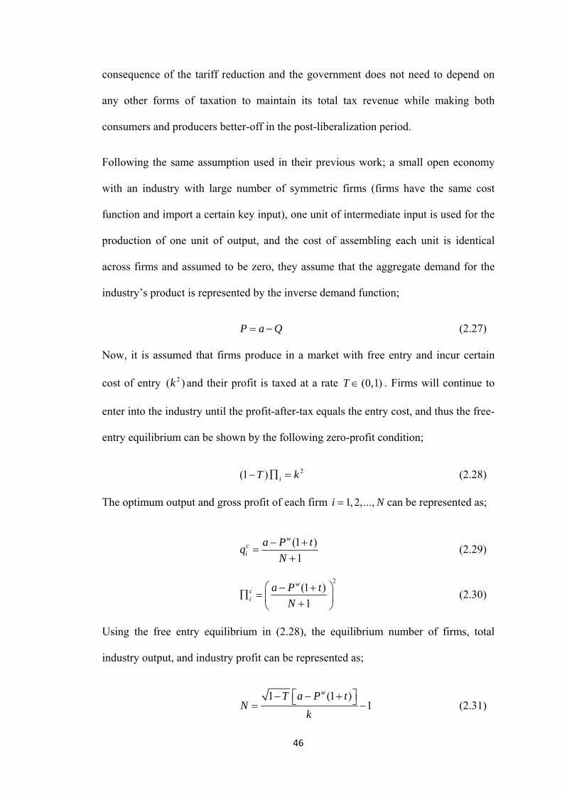
consequence of the tariff reduction and the government does not need to depend on
any other forms of taxation to maintain its total tax revenue while making both
consumers and producers better-off in the post-liberalization period.
Following the same assumption used in their previous work; a small open economy
with an industry with large number of symmetric firms (firms have the same cost
function and import a certain key input), one unit of intermediate input is used for the
production of one unit of output, and the cost of assembling each unit is identical
across firms and assumed to be zero, they assume that the aggregate demand for the
industry’s product is represented by the inverse demand function;
P a Q= − (2.27)
Now, it is assumed that firms produce in a market with free entry and incur certain
cost of entry and their profit is taxed at a rate 2( )k (0,1)T ∈ . Firms will continue to
enter into the industry until the profit-after-tax equals the entry cost, and thus the free-
entry equilibrium can be shown by the following zero-profit condition;
2(1 ) iT k− ∏ = (2.28)
The optimum output and gross profit of each firm 1, 2,...,i N= can be represented as;
(1 )1
wci
a P tqN
− +=
+ (2.29)
2
(1 )1
wci
a P tN
⎛ − +∏ = ⎜ +⎝ ⎠
⎞⎟ (2.30)
Using the free entry equilibrium in (2.28), the equilibrium number of firms, total
industry output, and industry profit can be represented as;
1 (1 )1
wT a P tN
k
⎡ ⎤− − +⎣ ⎦ (2.31) = −
46

1 (1 )
1
wc c
i
T a P t kQ Nq
T
⎡ ⎤− − + −⎣= =−
⎦ (2.32)
( )1 (1 )
(1 )
wc c
i
T a P t k kN
T
⎡ ⎤− − + −⎣ ⎦∏ = ∏ =−
(2.33)
From (2.29) and (2.30), it is obvious that tariff reduction will increase both output and
profit of individual firm and will consequently reduce the price of the product if the
number of firms remains fixed. With the assumption of free entry, new firms will
continue to enter into the industry until their profit-after-tax is equal to the entry cost,
. This will finally increase the equilibrium number of firms in the industry, total
industry output, and the gross industry profit as stated in equation (2.31) to (2.33).
2k
First, Haque and Mukherjee (2005) establish the condition under which the
government needs to use non-distortionary taxation (profit tax) to recover the revenue
loss, if there is any, as a result of tariff reduction. Thus, equation (2.34) presents the
condition whether there is any possibility that tariff revenue might increase or stay the
same after the tariff is reduced, without any change in the profit tax, T . Tariff
reduction means that . A Bt t<
w c w cA A BP t Q P t Q≥ B (2.34)
In previous work, the number of firms remains unchanged . Referring to
equation (2.11), tariff reduction reduces tariff revenue if and only if;
( )A BN N=
(1 )wA Ba P t t> + + (2.35)
If equation (2.35) is assumed to be satisfied, following equation (2.29), it ensures a
positive output of the entering firms. Using the expressions for c cA A iAQ N q= and
47

cB BQ N q= c
iB , and utilizing equation (2.31), (2.32), and (2.35) into equation (2.34), we
can re-arrange equation (2.34) to get a critical level of entry cost, , as follows; tk
( )1 1wA Bk T a P t t t⎡ ⎤≥ − − + + ≡⎣ ⎦ k (2.36)
Equation (2.36) proposes that, for any given profit tax rate, there always exists a level
of entry cost, such that tariff revenue will always increase following a reduction
in tariff rate. The reason underlying the above result is that tariff reduction reduces the
marginal cost of each firm and leads to an increase in profit. Higher profit attracts
more firms to enter into the industry and they continue entering until profit-after-tax
equals to the entry cost. This will lead to increase in import demand of intermediate
input and will consequently increase tariff revenue. However, tariff revenue would
fall for all
tk k≥
( )0, tk k∈ .
Second, Haque and Mukherjee (2005) establish the condition under which the
reduction in tariff revenue can be compensated for by an automatic increase in
industry profit for all entry costs ( )0, tk k∈ and leaving the profit tax rate, T ,
unchanged. From equation (2.33), for a given profit tax, when tariff is reduced, gross
industry profit will increase and finally lead to an increase in profit tax revenue. Thus,
if an increase in profit tax revenue (while keeping T fixed) dominates the reduction in
tariff revenue for , the total revenue will increase. This can be shown by the
following equation.
(0, tk k∈ )
c w c c w cA A A B BP t Q T P t Q T B+ ∏ ≥ + ∏
or, ( ) ( )c c w c cA B B B AT P t Q t Q∏ −∏ ≥ − A (2.37)
48

Using the expressions for c cA A iAN π∏ = and c
B B iN cBπ∏ = and utilizing equation (2.35),
we can re-arrange equation (2.37) to get a critical level of the entry cost in
which, for any value beyond this critical level, the government does not need to take
any compensatory measure by raising profit tax. This can be shown by the following
equation;
( )TRk
( )1 1
1
wA B TR
T a P t tk
T T
⎡ ⎤− − + +⎣≥+ −
k⎦ ≡ (2.38)
where . TR tk k<
Equation (2.38) proposes that, for any given profit tax rate, T , there always exists a
level of entry cost, , such that tariff revenue will decline but total revenue
will increase following a reduction in the tariff rate because an increase in profit tax
revenue dominates the reduction in tariff revenue.
[ , )TR tk k k∈
Last, Haque and Mukherjee (2005) consider the case where . From
equation (2.38), it is very obvious that for any , total revenue decreases since
an increase in profit tax revenue cannot offset the reduction in tariff revenue as a
result of the reduction of the tariff rate. In this case, the government can make up the
shortfall in its revenue by raising the profit tax rate from to . The revenue
recovered can be achieved only if an increase in the industry’s profit tax revenue is
higher than the shortfall in tariff revenue. This can be presented as;
[0, )TRk k∈
AT
TRk k<
BT
( )c c w c cA A B B B B A AT T P t Q t Q∏ − ∏ ≥ − (2.39)
Using the expressions for c cA A iAQ N q= , , c c
B BQ N q= iBc cA A iAN π∏ = and c c
B BN iBπ∏ =
and substituting them into equation (2.39), and assuming 0k = , equation (2.39) can
be re-arranged as;
49
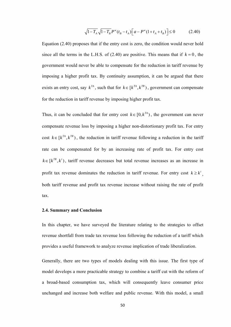
1 1 ( ) (1 )w wA B B A A BT T P t t a P t t⎡− − − − + + ≤⎣ 0⎤⎦ (2.40)
Equation (2.40) proposes that if the entry cost is zero, the condition would never hold
since all the terms in the L.H.S. of (2.40) are positive. This means that if , the
government would never be able to compensate for the reduction in tariff revenue by
imposing a higher profit tax. By continuity assumption, it can be argued that there
exists an entry cost, say , such that for , government can compensate
for the reduction in tariff revenue by imposing higher profit tax.
0k =
TAk [ , )TA TRk k k∈
Thus, it can be concluded that for entry cost , the government can never
compensate revenue loss by imposing a higher non-distortionary profit tax. For entry
cost , the reduction in tariff revenue following a reduction in the tariff
rate can be compensated for by an increasing rate of profit tax. For entry cost
, tariff revenue decreases but total revenue increases as an increase in
profit tax revenue dominates the reduction in tariff revenue. For entry cost ,
both tariff revenue and profit tax revenue increase without raising the rate of profit
tax.
[0, )TAk k∈
[ , )TA TRk k k∈
[ , )TR tk k k∈
tk k≥
2.4. Summary and Conclusion
In this chapter, we have surveyed the literature relating to the strategies to offset
revenue shortfall from trade tax revenue loss following the reduction of a tariff which
provides a useful framework to analyze revenue implication of trade liberalization.
Generally, there are two types of models dealing with this issue. The first type of
model develops a more practicable strategy to combine a tariff cut with the reform of
a broad-based consumption tax, which will consequently leave consumer price
unchanged and increase both welfare and public revenue. With this model, a small
50

open economy is considered with three related sectors including a representative
household, a perfectly competitive production sector, and a government. The model
considers the reduction of tariff in tradable commodities which is combined with a
point-for-point increase in the domestic consumption tax. A point-for-point
adjustment of the consumption tax is needed to exactly offset the impact of the tariff
reduction on the consumer price. The model does not only make a first attempt to
offer a formal theory of policy reform to offset the loss of revenue caused by tariff
reduction, but it also provides a remarkably simple and practicable way to reap the
efficiency gain from tariff reduction while improve the government’s revenue
position. However, the assumption underlying the model is perfect competition which
is far from the real economy. In addition, the model cannot be extended to deal with
the reduction of tariffs on intermediate goods used to produce tradable goods since it
is not possible to offset the tariff reduction by increasing consumption tax without
affecting the consumer price.
The second type of model examines the reduction of a tariff on an intermediate input
because trading in intermediate inputs accounts for a large share in world trade. The
model investigates whether the government can make up a shortfall in revenue if the
government reduces the tariff on an intermediate input under imperfect competition,
while the make up by using profit tax must ensure that both consumers and producers
must be better off in the post-liberalization period. The model shows that only when
the industry is a monopoly can it be certain that raising the profit tax alone will
generate enough revenue to make up for the shortfall following the tariff reduction.
This strategy can also ensure that consumers and producers are better off in the post-
liberalization period as a result of an increase in welfare. However, a model dealing
with product differentiation shows that there always exists degree of product
51

differentiation such that the government can achieve these objectives for any finite
number of firms in the industry. The model suggests that when the products are
sufficiently differentiated, each firm becomes a near monopolist for its products and
the government can use higher profit tax revenue to offset the shortfall of tariff
revenue. A further developed model dealing with the entry costs shows that the
possibility that the government can use a profit tax as a compensatory measure for the
loss of tariff revenue may alter depending on the range of entry cost, from high to
low. The model shows that a sufficiently large entry cost will generate higher tariff
revenue and profit tax revenue due to the entry of new firms into the industry, and
hence the market itself will compensate for any shortfall in revenue as a consequence
of the tariff reduction and the government does not need to depend on any other forms
of taxation to maintain its total tax revenue while making both consumers and
producers better-off in the post-liberalization period. However, with a low entry cost,
the government would never be able to compensate the reduction in tariff revenue by
imposing higher profit tax.
52

Chapter 3
TRADE LIBERALIZATION AND
TRADE PERFORMANCE IN THAILAND
53
3.1. Introduction
The impact of trade liberalization on the volume of trade in developing countries
remains an unsettled question in economics, although a number of related literatures
have been recently studied (see, for example, Mouna and Ahmad Reza (2001);
Thomakos and A. Ulubasoglu (2002); Santos-Paulino and Thirlwall (2004); Pacheco-
Lopez (2005); Pacheco-Lopez and Thirlwall (2006); Wu and Zeng (2008)). Within
this body of knowledge, numerous effort has been gone into estimate the import and
export demand functions for many developing countries and the results have been
mixed. This is unfortunate since import and export elasticities are generally highly
dependent on income, relative prices, and trade policy in particular. The analysis of
import demand and export demand is necessary to understand the effects of trade
liberalization may have a wide range of effects on a country’s economy. For example,
if trade liberalization policies induce a higher volume of imports than exports, then
this may adversely affect the balance of payments of the country in question. Given
such an adverse influence, it is thus important to establish import and export demand
functions. This chapter seeks to estimate the likely impact of trade liberalization
policies on the volume of imports and exports using aggregated import and export
demand functions in Thailand for the period 1960 to 2007.
This chapter has two main purposes. In the first place, within the international trade
literature, it is generally found that trade relationships fluctuate over time because
many macroeconomic variables, which determine trade relations, are non-stationary
in nature. In addition, trade relationships are subject to both gradual and sudden
changes over time (Goldstein and Khan, 1985). Gradual changes are regarded as
changes in the macroeconomic environments which potentially have an impact on
international trade in long term, such as the process of economic development, the
54

growth of the country, and the consequences of changes in government trade policies.
Sudden changes are regarded as changes in macroeconomic variables which have an
immediate effect on international trade, such as fluctuations in exchange rates and a
substantial increase in oil price. Considering these concerns, our interest is to
investigate whether there exists a long-run relationship between trade and its major
determinants. A thorough understanding of the determinants behind imports and
exports is necessary for policy makers to formulate appropriate trade policy.
The second aim of this chapter is to analyze the impact of trade liberalization on the
volume of imports and exports in Thailand. Since 1960, many developing countries
have switched from a closed economy to a more opened economy by inducing free
trade policies in the hope that liberalization will bring an improvement on overall
economic performance and address balance of payments difficulties.3 In line with this
general trend, Thailand has formally introduced trade liberalization policy since its
accession to the AFTA in 1992 and the WTO in 1995, though its tariffs have been
gradually reduced over the time. By opening the country, Thailand primarily hopes to
achieve better export performance and hence alleviate the ongoing trade deficit
problem. Theoretically and empirically, trade liberalization is generally found to be
positively associated with the volume of imports, while it does not lead to an increase
in the volume of exports in the same proportion. From the UNCTAD Trade and
Development Report 1999, trade liberalization has often contributed to a widening of
the trade deficit in developing countries in general. For most developing countries, the
average trade deficit in the 1990s was higher than in the 1960s-1970s by
approximately 3-5 percentage of GDP. However, in the case of Thailand, it is found
3 This is based on the history of the GATT in which its second phase (lasted from 1959 to 1979) and third phase (lasted from 1986 to 1993) and the replacement of the WTO, have focuses on the reduction and elimination of tariffs.
55

that the trade balance in the post-liberalization era has improved rather than worsened.
For almost all years in the post-liberalization period, the volume of exports has
exceeded the volume of imports. Still, a substantial increase in the volume of exports
since the mid 1990s, which overwhelms an increase in the volume of imports, is
mainly due to the currency depreciation after Asian financial crisis. Accordingly, in
this chapter we examine whether trade liberalization has had any impact on the import
and export performance of the Thailand economy.
Thus, with this background, the aims of this chapter are to assess empirically the
major determinants of import and export demand functions in Thailand using
cointegration technique to estimate the long-run equilibrium relationship and error-
correction model to examine the dynamic behaviour. We, then, aim to estimate the
income and price elasticities from both import and export demand functions. Finally,
we need to ascertain the impact of trade liberalization on the volume of imports and
exports in both the short run and the long run.
The rest of this chapter is divided into five main sections. Section 2 provides a
comprehensive description of Thailand’s trade profile and its trade policies as well as
background information on the characteristics of Thailand’s imports and exports over
the studying period. Section 3 briefly reviews the related theoretical literature, and
outlines the empirical studies on import and export demand function. Section 4 deals
with model specification, data sources, and methodology used in this study. Section 5
discusses the results of the estimation procedures. The chapter ends with some brief
summaries and concluding remarks in section 6.
56

3.2. Thailand’s Import and Export and Trade Policies
Thailand’s International Trade Sector
Since 1960, international trade has become more substantial in terms of its share of
Thailand’s Gross Domestic Product (GDP). As shown in Figure 3.1, trade (defined as
the summation of imports and exports) as a percentage of GDP has steadily increased
over time. From only 33 percent of GDP in 1960, trade accounted for almost 150
percent of GDP in 2005, though it went down to approximately 130 percent of GDP
in 2007. Obviously, the international trade sector has become increasingly important
for Thailand.
Figure 3.1: Trade as a Percentage of GDP
0
50
100
150
200
1960
1962
1964
1966
1968
1970
1972
1974
1976
1978
1980
1982
1984
1986
1988
1990
1992
1994
1996
1998
2000
2002
2004
2006
% o
f GD
P
Year
Source: World Bank; World Development Indicators (December 2008)
From Figure 3.2, trade in both goods and services have shown impressive rates of
growth. The proportion of trade in goods to GDP rose from only about 30 percent in
1960 to approximately 105% in 2007, reaching its peak about 122% in 2005. The
proportion of trade in services to GDP also rose gradually from only 3 percent in 1960
to 27% in 2007.
57

Figure 3.2: Trade in Goods and Services as a Percentage of GDP
020406080
100120140
1960
1962
1964
1966
1968
1970
1972
1974
1976
1978
1980
1982
1984
1986
1988
1990
1992
1994
1996
1998
2000
2002
2004
2006
Perc
enta
ge o
f GD
P
Year
Trade in Goods
Trade in Services
Source: World Bank; World Development Indicators (December 2008)
Over the studying period, the structure of Thailand’s exports has considerably
changed. From Figure 3.3, agricultural exports began to decrease in the early 1960s
and have declined substantially for the whole period, while manufactured exports
began to increase in the late 1960s and have dramatically risen since then. In 1960,
agricultural exports accounted for almost 40 percent of merchandise exports, while
manufactured exports only made up 2 percent. Thailand started promoting export-
oriented industries in the early 1970s. Exports of manufactures goods have turned out
to be higher than exports of agricultural goods since 1975. In 2007, manufactured
exports reached the highest point, accounting for about 80 percent of merchandise
exports, while agricultural raw materials exports, decreasing over the period,
computed only 5 percent. This sharp rise in manufactured exports and fall in
agricultural exports is another remarkable feature of Thailand’s exports.
58

Figure 3.3: Share of Agricultural and Manufactures exports in Merchandise exports
0
20
40
60
80
100
1960
1963
1966
1969
1972
1975
1978
1981
1984
1987
1990
1993
1996
1999
2002
2005%
of m
erch
andi
se e
xpor
ts
Year
Agricultural raw materials exports
Manufactures exports
Source: World Bank; World Development Indicators (December 2008)
Considering imports, from Figure 3.4, it is found that imports of manufactured goods
are much higher than imports of agricultural products. Although Thailand adopted an
import-substitution policy in 1958 and switched from import-substitution
industrialization to export-oriented industrialization in later years, imports of inputs,
materials, and capital goods show no obvious sign of declining. In average,
manufactured imports accounted for approximately 70 percent of merchandise
imports, whereas agricultural imports made up only 3 percent of merchandise imports.
This reflects the fact that Thailand is a big importer of manufactured products in
which these products are needed in the production process of medium to high-
technological goods. It also reflects the fact that Thailand has a high consumption in
imported luxury goods.
59

Figure 3.4: Share of Agricultural and Manufactures imports in Merchandise imports
0
20
40
60
80
100
1960
1963
1966
1969
1972
1975
1978
1981
1984
1987
1990
1993
1996
1999
2002
2005
% o
f mer
chan
dise
impo
rts
Year
Agricultural raw materials imports
Manufactures imports
Source: World Bank; World Development Indicators (December 2008)
Figure 3.5 provides the picture of Thailand’s imports and exports from 1960 to 2007.
Before 1997, imports exceeded exports in almost all years. The main reason is that
Thailand’s exports are highly dependent on the imports of raw materials, machinery,
and crude oil. In addition, the high consumption of imported luxury goods, when the
economy was booming, resulted in the high demand for imported goods.4 However, it
is very obvious that exports substantially increased during 1997 and 1998, while
imports slightly declined in 1998. Exports jumped from 39 percent of GDP in 1996 to
48 percent of GDP in 1997 and 59 percent of GDP in 1998. A substantial increase in
exports was mainly due to the currency depreciation after the financial crisis in 1997.
The majority of the growth in exports over the past decade was in manufactured
goods, particularly high-tech products and the major source countries being Japan and
NAFTA (North American Free Trade Agreement) countries, especially United States
4 According to Siamwalla (1999) and Warr (2005), we can divided Thai economy into 4 sub periods including; I. 1960‐1985 (Pre‐boom); is the period that Thai economy got its foundation right by investing in
physical infrastructure which later help made economic growth high and stable. However, there was still high macroeconomic uncertainty.
II. 1986‐1996 (Boom); is the period that Thailand had an extraordinary high economic growth. III. 1997‐1998 (Crisis); is the period that Thailand and Many ASEAN countries encountered with
economic and financial crisis. IV. 1999‐Present (Post‐crisis); is the period that Thailand has recovered and challenged with world
economic fluctuation.
60

of America. Due to the export jump in 1997, imports have turned out to be lower than
exports from that year. However, the impact of currency depreciation on imports
seems to be only one year after the crisis. Since 1999, imports have risen continually,
as usual. Much of the increase in imports is in raw materials, intermediate goods, and
capital goods, such as mineral and metal products, chemicals and plastic materials,
electronic parts, and industrial machinery, industrial tools and parts, which are
required in the production process of exports, rather than consumer goods and a
substitution for domestic production. The main import sources of countries are Japan,
United States, and China.
Figure 3.5: Imports and Exports of Goods and Services
01020304050607080
1960
1962
1964
1966
1968
1970
1972
1974
1976
1978
1980
1982
1984
1986
1988
1990
1992
1994
1996
1998
2000
2002
2004
2006
% o
f GD
P
Year
Imports of goods and services
Exports of goods and services
Source: World Bank; World Development Indicators (December 2008)
From Table 3.1, it can be seen that the balance of trade has made the greater
contribution to the current account position. This, again, reflects the importance of the
international trade sector in Thailand. From 1975 to 1996, Thailand suffered from a
trade deficit, and hence a current account deficit in almost all years. The impact of
currency depreciation was immediately seen in the trade balance and the current
account. In 1997, trade balance turned out to have a surplus after ten years of a deficit.
In 1998, net trade surplus jumped to over 16,000 million US dollars, accounting for
61

approximately a 10-fold increase from previous year. After 1996, Thailand has a trade
surplus, although the surplus has dropped in some years.
Table 3.1: Details in Current Account of Thailand, 1975-2007
Year Million US$ Net current
transfers Net income Net trade in goods
1975 80.67 10.99 -672.69 1976 46.86 -53.68 -193.14 1977 39.51 -38.14 -783.97 1978 40.13 -148.22 -858.37 1979 58.86 -277.87 -1,550.34 1980 210.14 -229.31 -1,902.47 1981 167.52 -502.43 -2,028.95 1982 183.09 -514.56 -730.56 1983 277.78 -227.09 -2,861.12 1984 174.97 -440.24 -1,897.74 1985 165.24 -597.13 -1,332.14 1986 224.73 -816.71 388.38 1987 223.77 -829.67 -424.46 1988 236.28 -894.37 -2,074.42 1989 246.25 -780.52 -2,916.11 1990 213.30 -853.39 -6,750.84 1991 260.90 -1,075.39 -5,989.18 1992 645.60 -1,707.72 -4,161.02 1993 749.64 -1,406.25 -4,288.13 1994 1,127.56 -1,730.80 -3,699.83 1995 486.51 -2,113.63 -7,968.06 1996 759.72 -3,385.33 -9,488.17 1997 478.81 -3,480.24 1,571.58 1998 414.39 -3,567.14 16,237.90 1999 353.18 -2,990.96 14,013.30 2000 585.86 -1,381.30 11,700.61 2001 600.73 -2,457.16 8,543.46 2002 603.42 -3,663.36 9,043.92 2003 940.93 -4,973.24 11,174.59 2004 2,131.49 -6,120.42 10,785.24 2005 3,003.63 -7,173.50 3,387.69 2006 3,368.01 -6,843.50 13,843.67 2007 3,938.05 -5,709.98 25,959.75
Source: World Bank; World Development Indicators (December 2008)
Figure 3.6 shows the declining trend in both Thailand and the world’s average tariff
rates. In 1960, Thailand’s average tariff rate was initially very high, approximately
62

70%, while the world’s tariff rate was about 55%. From Figure 3.6, the average tariff
rates of both Thailand and the world have gradually decreased over time. During the
mid 1980s to the early 1990s, the gap between Thailand’s average tariff rate and the
world’s tariff rate was very high because the country implemented the protection
policies for the domestic substitutes industries. However, in 1994, there was a steep
decline in Thailand’s average tariff rate, from approximately 46% in 1993 to 23% in
1994. This is mainly due to an agreement made with ASEAN and GATT for the
country to become a member of AFTA in 1992 and the WTO in 1995. Since then,
Thailand’s average tariff rate has been only little higher than that of the world. In
2007, Thailand’s average tariff rate was reduced to only 10%, while the world’s
average tariff rate was recorded at 8%.
Figure 3.6: Trends in Average Tariff Rates
010203040506070
1960
1962
1964
1966
1968
1970
1972
1974
1976
1978
1980
1982
1984
1986
1988
1990
1992
1994
1996
1998
2000
2002
2004
2006
Perc
ent
Year
Thailand's Average Tariff Rate
World's Average Tariff Rate
Source: United Nations Conference on Trade and Development (UNCTAD), 2007
In order to investigate the trend between imports and the tariff rate, we plot the graph
of the share of imports in GDP against Thailand’s average tariff rate. Figure 3.7
shows that there is a linkage between the country’s average tariff rate and the share of
imports in GDP. By looking at the diagram, there is evidence of a negative
relationship between the two variables.
63

Figure 3.7: Thailand’s Import Share of GDP and Thailand’s Average Tariff Rate
0
10
20
30
40
50
60
70
0 10 20 30 40 50 60 70 8Thailand
's Average
Tariff Rate
(%)
Imports as a percentage of GDP
0
Source: WDI and UNCTAD
Trade liberalization was not only associated with the country’s import share, but there
also seemed to be a relationship with Thailand’s export share. Similarly, we plot the
graph of the share of exports in GDP against world’s average tariff rate. Figure 3.8
shows that world’s tariff reductions seemed to be associated with an increase in the
share of export in GDP.
Figure 3.8: Thailand’s Export Share of GDP and World’s Average Tariff Rate
0
10
20
30
40
50
60
0 10 20 30 40 50 60 70 8World's Average
Tariff Rate
(%)
Exports as a percentage of GDP
0
Source: WDI and UNCTAD
Having described the trade characteristics of Thailand, we now give a brief outline of
Thailand’s trade policy.
64

Thailand’s Trade Liberalization Policy
By implementing an open trade regime in its international trade, Thailand has been
recognized as one of the fastest growing economies in the world. With the global
trend, Thailand has used many trade measures as instruments to strengthen the
competitiveness of domestic industries to compete in the world market. By pursuing
the policy of freer trade-led-development, Thailand has participated in many
international forums such as the Uruguay Round of GATT, the Asia-Pacific
Economic Cooperation forum (APEC), and the ASEAN Free Trade Area (AFTA).
Another important step to free trade was its accession to the World Trade
Organization (WTO) on 1 January 1995. Since then, Thailand has implemented
various measures in compliance with its commitments in the WTO. The tariff system
has been restructured while many laws have been enacted in accordance with the
Trade Related Aspects of Intellectual Property Rights (TRIPs) agreement. Most of the
goods and services sectors are going through the liberalization process. Many
quantitative restrictions on various types of agricultural products have been eliminated
and replaced by tariff measures in line with the procedure prescribed in the agriculture
agreement. In short, Thailand has attempted to open its economy by implementing
many laws and regulations as its part of commitment to the WTO. As stated earlier,
Thailand is also participating in many regional cooperation schemes. As one of the
countries in the Asia-Pacific region, Thailand has closely followed development in
APEC and tried to ensure that this forum is consistent with multilateralism, the
concept created by the WTO. As one of the leading nations in ASEAN, Thailand has
played an important role in the establishment of the ASEAN Free Trade Area (AFTA)
which encourages free trade and cooperation among neighbouring countries in this
region.
65

a) The Uruguay Round and the WTO
With the success of the Uruguay Round negotiation, Thailand believed that
trade negotiations under GATT, the establishment of the WTO and the
improvement of international trade rules and negotiations would create a more
stable economic environment, greater economic development, and higher
income from trade. By being involved in the Uruguay Round and the creation
of the WTO, the main objectives are to assure greater trade liberalization
through the reduction and elimination of both tariff and non-tariff barriers, to
improve the effectiveness of the rules and regulations governing international
trade, to bring about fairness and transparency in the market, and to prevent
new trade barriers that may obstruct international trade. With these beliefs,
Thailand became a member of GATT in October 1982 and the 59th founding
member of the WTO on 28 December 1994.
Under the WTO agreements, Thailand has to reduce an average of 24 percent
of tariffs on agricultural products. The country also needs to eliminate non-
tariff barriers for 23 agricultural products and convert these NTBs into tariff
measures in accordance with the tariffication process. In addition, tariffs of
over 4,000 items of industrial and fisheries products have to be reduced during
this process and this results in an average of 28 percent of tariff reduction.
b) Asia-Pacific Economic Cooperation (APEC)
Created in 1989, Asia-Pacific Economic Cooperation (APEC) is aim to
improve cooperation, trade, and investment in the region. In the context of
APEC, liberalization, trade and investment facilitation, and technical
cooperation in the APEC region are considered as a priority. Under APEC, the
Free Trade Area of the Asia-Pacific Region (FTAAP) has been proposed by
66

the member nations in which its scope is not only focusing on the reduction of
tariffs and other trade restrictions, but also the creation of a free trade zone.
The development of FTAAP is now under study and may take many years to
reach the conclusion. Considering Thailand, its policies toward APEC are
made compatible with its commitment under the WTO. Under the 1994 Bogor
declaration, Thailand has to reduce its tariffs to below 5 percent by 2020.
c) The ASEAN Free Trade Area (AFTA)
Thailand is one of the founding members of ASEAN, which later established
the ASEAN Free Trade Area (AFTA). The agreement was signed in Singapore
on 28 January 1992. The main objective in the establishment of AFTA is to
reduce and eliminate intra-regional tariffs on all manufactured items including
capital goods and processed agricultural products to 0-5 percent and remove
non-tariff barriers over 15 years, starting from the beginning of 1992 and
finalizing by the end of 2008. As for Thailand, there are two packages of tariff
reductions under AFTA which have been commenced on 15 February 1992.
For the first package, from 1992, Thailand has reduced the tariff rates up to 30
percent on all manufactured items imported from ASEAN, except for certain
sensitive products such as petrochemical, plastic products, and televisions. For
the second package, from the end of 1994, Thailand has to reduce further tariff
rates of products under the Fast Track Programme in accordance with the tariff
reduction schedule as follows;
From 26-30 percent to 25 percent
From 21-25 percent to 20 percent
From 15-20 percent to 15 percent
From 11-14 percent to 10 percent
67

From 6-10 percent to 5 percent
However, under the meeting held in September 1994 in Chiang Mai, in view
of the present economic challenges and the conclusion of the Uruguay Round
multilateral negotiations, ASEAN has agreed to shorten the time frame that
was initially set from 15 to 10 years. That is all reduction, elimination and
removal of tariff and non-tariff barriers must be accomplished by 1 January
2003 instead of 2008.
In summary, as Thailand’s economic performance has become more increasingly
dependent on international trade, the country has joined a number of trade agreements
with other countries. With the hope to achieve the benefit of attaining economic
prosperity, Thailand has realized the importance of liberalization and open trade to the
country’s development.
3.3. General Review: Empirical Studies on the Relationship between Trade
Liberalization, Imports, and Exports
For several decades, the determinants of trade, the behaviour of import and export
demand functions have been analyzed in many different studies. Among an
impressive range of empirical studies, the most important works include Houthakker
and Magee (1969), Khan (1974), Murray and Ginman (1976), Salas (1982), Melo and
Vogt (1984), Goldstein and Khan (1985), Bahmani-Oskooee (1986), Sarmad (1989),
Clarida (1994), Carone (1996), Sinha (1997), Senhadji (1998), Thomakos and
Ulubasoglu (2002), Aydin et al (2004), Santos-Paulino and Thirlwall (2004), Dutta
and Ahmed (2004), Pacheco-Lopez (2005), Dash (2006), Huseyin (2006), and Aliyu
(2007). For instance, Houthakker and Magee (1969) investigate demand elasticities
for both imports and exports with respect to income (GNP in constant prices) and
68
prices for the United States comparing with a number of developed countries. Using
the ordinary least-squares (OLS) method and annual data over the period 1951-1966,
they found that the income elasticity of demand for imports for the U.S. and other
developed countries is about the same, while the income elasticity of demand for
exports for the U.S. is relatively low, resulting in trade balance problem as the world
grows. The price elasticities estimated for all countries appeared to be very low. Khan
(1974) examined the effect of prices on trade flow by estimating import and export
demand functions using annual data for 15 developing countries over the period 1951-
1969. By using two-stage least-squares method, he found that prices have a significant
and substantial impact on both import and export demand for all countries used in his
study. Murray and Ginman (1976) estimated the traditional aggregate import demand
for the U.S. over the period 1950 to 1964 by using quarterly data. They found that the
income elasticity varied from 0.96 to 1.94 whereas the import price elasticity was
approximately equal to one. Salas (1982) investigated the structure of Mexican
imports for the period 1961 to 1979 by focusing on private sector imports. He also
determined the possibility of a structural break in the import demand functions for the
period 1961-1977 and 1961-1979, since Mexico has changed its trade policies from
traditionally protective international trade policies from 1976. He found that imports
of Mexico were highly dependent on relative import price but had a very low response
to income changes. The price elasticity was improved when the country adopted
liberalization policies, while the income elasticity was dropped in the liberalized
period. Melo and Vogt (1984) estimated real income and relative price elasticities of
demand for imports of Venezuela by using disaggregated annual data covering the
period 1962 to 1979. At the aggregate level, the price elasticity was very high (-
2.086), comparing with other studies. The income elasticity was also found to be
69

higher than unity (1.879). At the disaggregated level, income and price elasticities for
most goods were higher than unity, except for manufacturing imports which both
price and income were highly inelastic. Goldstein and Khan (1985) provided a
comprehensive survey of the literature on the determinants of trade focusing on the
role of income and prices and estimated import demand function for 14 developed
countries. They found that income seemed to have higher impact on import demand
than prices. Bahmani-Oskooee (1986) used quarterly data from 1973 to 1980 period
and provided the estimates of aggregate import and export demand functions for
seven developing countries. He also provided estimates of price and exchange rates
response patterns by introducing a distributed lag structure on the relative prices and
on the effective exchange rate. After estimating import and export demand functions
using the Almon procedure, it is found that developing countries generally were price
inelastic, but income elastic concerning demand for imported goods. However, both
income and price appeared to be highly inelastic for all countries under study. Sarmad
(1989) estimated import demand functions for total imports of Pakistan for the period
1959 to 1986 at both the aggregate and disaggregate levels. He found that the
aggregate elasticities for both income and relative price were lower than unity (0.923
for income elasticity and -0.415 for price elasticity). At the disaggregate level, the
income elasticities ranged from 1.4 to as low as 0.45, depending on the type of import
goods. Similarly, the disaggregate price elasticities ranged from -1.2 to -0.42.
More recent studies have applied cointegration and error-correction technique in the
study of import and export demand functions. For example, Clarida (1994) derived an
econometric equation used for estimating the parameters of the demand for imported
nondurable consumer goods of the U.S. by using quarterly data covering the period
1967 to 1982. He estimated a long-run equilibrium relationship between consumer
70

goods imported, relative price of imports, and consumption of domestically produced
goods and found that all these variables are cointegrated. The long-run price elasticity
of import demand was estimated to average -0.95, while the elasticity of import
demand with respect to a permanent increase in real spending was equal to 2.15.
Carone (1996) estimated aggregate import demand for total and non-oil merchandise
imports of the U.S. over the period 1970 to 1992 using cointegration and error-
correction approaches. He found a statistically significant long-run relationship
between the volume of imports and real income and relative prices. Sinha (1997)
estimated import demand function for Thailand by using annual data covering the
period 1953 to 1990 and applying cointegration and ECM approaches. He found that
both price and income were inelastic in the short run. Relative import price was still
inelastic in the long run while income turned out to be very elastic in the long run.
Senhadji (1998) estimated a structural import demand function for 77 developing and
industrial countries from 1960 to 1993 by using cointegration and the fully modified
ordinary least squares estimator (FMOLS). He found that imports seem to be inelastic
in the short run but are more responsive to relative prices in the long run (average
short-run price elasticity is -0.26, while average long-run price elasticity is -1.08).
Similarly, he found that imports respond more to income in the long run than in the
short run (average long-run income elasticity is equal to 1.45, whereas average short-
run income elasticity is equal to 0.45). He also found that industrial countries tend to
have higher income elasticities and lower price elasticities than developing countries.
Aydin et al (2004) developed a single equation and a vector auto-regression
framework and used quarterly data covering the period 1987 to 2003 to estimate
import demand for the Turkish economy. They found that both long-run and short-run
income elasticities were higher than unity (1.999 and 1.188 for long-run and short-
71

run, respectively), while both long-run and short-run price elasticities were lower than
unity (-0.402 for long-run and -0.527 for short-run). Dash (2006) investigated the
behaviour of the import demand function for India using annual data from 1975 to
2003. Economic activity (GDP), import price, foreign exchange reserves, and price of
domestically produced goods were included as determinants of aggregate import
demand. It is found that the aggregated import volume was cointegrated with all
variables stated earlier and the import demand of India was largely explained by price
of domestically produced goods, GDP, lag of import and foreign exchange reserves.
Huseyin (2006) estimated an aggregate demand function for Turkey using monthly
data during the period 1994 to 2003 and applied cointegration and error correction
modeling approaches to investigate the long-run relationship and the dynamics of
short-run adjustment process. It is found that there was a unique equilibrium
relationship existing among the real quantity of imports, relative prices, and real GNP.
The value of income elasticity of import demand was lower than price elasticity,
suggesting that Turkey’s imports were sensitive more to import price changes than to
income changes. In addition, the speed of adjustment to long-run equilibrium was not
very high. Aliyu (2007) examined the determinants of import and export demand
functions for Nigerian economy using data covering the period of 1970 to 2004. It is
found that current income had very little influence on both imports and exports while
lag income highly affected both, especially on export demand. Nigeria’s exports
expanded substantially because of very high income elasticity. In addition, the price
elasticity of imports appeared to be higher than price elasticity of exports.
There are many studies investigating the role of trade liberalization on trade flow. The
analysis was generally done by including the measures of trade liberalization into both
import and export demand functions. For example, Thomakos and Ulubasoglu (2002)
72

analyzed the impact of trade liberalization on import demand of Turkish economy by
using annual disaggregated data for the period 1970 to 1995 covering 26 industries. In
order to analyze the impact of trade liberalization, they tested for different elasticities
over “closed” and “open” economy periods, and found that the effects of the trade
reforms of the 1980s were significant for a number of industries. The elasticities
estimated from many types of products were found to have changed notably as a
result of liberalization. Santos-Paulino and Thirlwall (2004) used panel data analysis
to examine the impact of trade liberalization on exports, imports, and the balance of
payments for 22 developing countries that have adopted trade liberalization policies
since the mid-1970s. Using different techniques such as the fixed effects and
generalized method of moments (GMM) for panel data analysis, they found that
reductions in export and import duties had significantly affected the growth of exports
and imports, with the impact on import growth greater. The impact of a more
liberalized trade regime raised import growth by more than exports. They also found
that liberalization increased income and price elasticities of both the demand for
imports and for exports. However, trade liberalization increased the price elasticity of
demand for imports greater than for exports, and hence the balance of trade was
possibly deteriorated after trade liberalization. They also suggested that the impact of
liberalization differed depending on the level of initial protection of the country. Dutta
and Ahmed (2004) investigated the behaviour of Indian aggregate imports during the
period 1971 to 1995. In order to capture the effect of the import liberalization policy
on import demand, they included a dummy variable with a value 1 for 1992-1995, the
liberalization period. They found that aggregate import volume was cointegrated with
relative import prices and real GDP. In the estimated ECM, import prices, lags of real
GDP and a liberalization dummy were found to be important determinants of import
73

demand function for India, with quite a slow speed of adjustment to equilibrium.
Import demand in India was largely explained by real GDP but appeared to be less
sensitive to import price changes, implying the noncompetitive nature of India’s
imports. An estimate of liberalization dummy was equal to only 0.14, showing little
effect of import liberalization policy on aggregate import volume. Pacheco-Lopez
(2005) investigated the impact of trade liberalization, during the mid 1980s from the
participation of the North American Free Trade Agreement (NAFTA) on exports,
imports, the balance of payments and growth in Mexico using annual data covering
the period 1970 to 2000. In order to identify the long-run relationship between the
dependent and independent variables, an autoregressive distributed lag (ARDL)
estimation technique were adopted in his study. He used a liberalization dummy to
capture the impact of trade liberalization. On export side, he found that export growth
responded substantially to the growth of the U.S. economy, but the price elasticity of
Mexican exports is quite low. NAFTA was found to have no impact on Mexican
export performance. On the import side, he found that import growth responded
substantially to both income and price changes. It is found that NAFTA had a
significant positive impact on import growth.
3.4. The Model and Methodology
In this study, we firstly apply the traditional import (export) demand functions and
then use the Autoregressive Distributed Lag (ARDL) model to estimate the short-run
and long-run elasticities in Thailand’s import (export) demand over the period 1960-
2007. We also compare these estimates with the estimates obtained using
cointegration techniques and an ECM.
74

3.4.1. The Model Specification and Equations
Although there is a large amount of literature on the import and export demand
modelling in general, the question how import and export models are appropriately
specified is still of interests. Although the specification of the models depend on a
number of factors, Goldstein and Khan (1985) suggested that the most important
things should be considered are the purpose of modelling exercise, the type of the
good being trade, institutional framework under which trade takes place, and the
availability of data. From trade theory, there are two basic models often used in the
studies of international trade; model of perfect substitutes and model of imperfect
substitutes. On one hand, perfect substitution model assumes perfect substitutability
between domestic and foreign goods. Thus, under the key assumption of perfect
substitution, a country could only be either an exporter or an importer of a traded
good, but not both. Since this is not observed in the real world, the perfect substitution
model is less popular in the empirical studies than the imperfect substitution model.
However, the perfect substitution model is typically used in the case of highly
disaggregate data set. On the other hand, the fundamental assumption underlying the
imperfect substitution model is that neither imports nor exports can be considered
perfect substitutes for the domestic products. This model is thus more realistic and is
more suitable for the case of aggregate data.5
Regarding the demand-supply relationships in the export and import equations, theory
suggests that one should emphasize the simultaneous relations between quantities and
prices, and hence demand and supply of import (export) equations should be
simultaneously solved in the system in order to avoid any possible biased results.6
5 See Goldstein and Khan (1985) 6 See Stern, Francis and Schumacher (1976)
75

However, like many other studies, since we concentrate on the estimation of import
and export demand equation, another important assumption must be applied to the
supply relationships. Typically, it is assumed that the import and export supply price
elasticities facing any individual country are infinite. The important advantage of this
assumption is that it allows the estimation of the import and export demand equations
by using single-equation method, in which the price variables are treated as
exogenous variables. However, Goldstein and Khan (1978) pointed out the drawback
of this assumption that although infinite price elasticity of supply may be justified in
the case of import supply, it seems to be unreasonable in the case of the supply of
exports of a small open economy. They argued that if the world demand for the goods
from a certain small individual country substantially increases, the country will not be
able to meet the demand without changing in price of exports (unless there exist large
idle resources). Still, the assumption of infinite price elasticity is necessary for our
analysis and must be hold in this study.
Following the relevant literature (see, for example, Houthakker and Magee (1969);
Leamer and Stern (1970); Khan (1974); Goldstein and Khan (1985); Carone (1996);
Bahmani-Oskooee and Niroomand (1998); and Santos-Paulino and Thirlwall (2004)),
we use the standard import and export demand functions to analyze the impact of
trade liberalization on the volume of imports and exports for Thailand. The standard
specification of the import and export demand models is similar to any other demand
model. The quantity of imports and exports demanded will be treated as endogenous
variables while the relative price of imports (price of imported goods relative to the
price of domestic goods), the relative price of exports (price of exported goods
relative to the world export price), world’s real income and country’s real income will
76

be considered as exogenous variables. By assuming the price and income elasticities
of demand are constant over time, the import function can be specified as follows:
1
2
aaM
tD t
PtM A
P⎡ ⎤
= ⎢ ⎥⎣ ⎦
Y (3.1)
where tM is the volume of imports at time t; A is a constant; ( )M D tP P denotes
relative import prices at time t; is the level of country’s income at time t. tY
There are still other assumptions underlying the imperfect substitute model. We
assume that the import demand is always equal to the level of imports ( )dM M= so
that we are able to apply the demand function in our study. Another basic assumption
is that, by using the relative price as a determinant, we assume that there is no money
illusion, homogeneity implying in prices.7
Regarding the appropriate specification of import demand, there is no theory
providing a specific functional form for this demand function. However, Thursby and
Thursby (1984) tested specifications of import demand and concluded that the log-
linear form is more desirable than the linear form. Other advantages of the logarithmic
form are their convenience and the ease of interpretation.8 Thus, following previous
studies9, taking the logs of the above function, the import function can be transformed
into logarithmic form as follow:
0 1 2ln ln lnt t t tM a a Y a RPM u= + + + (3.2)
where is the relative price. However, Goldstein and Khan (1976) have argued
that if imports of the country are considered as the difference between consumption
RPM
7 See Carone (1996) for more details 8 See Carone (1996) 9 See Khan and Ross (1977) and Boylan et al. (1980) for example
77

and production of domestically produced import substitutes, production may rise
faster (slower) than consumption in response to a rise (fall) in real income. Therefore,
imports could fall (rise) as real income increase, resulting in a negative (positive) sign
for income elasticity.
In order to capture the impact of trade liberalization on the import demand function,
we modify the basic model by including Thailand’s average tariff rates and a
liberalization dummy variable
(TT )
)(LIB . The dummy variable takes the value 1 from
1992 and 0 otherwise; this is based on Thailand joining the ASEAN Free Trade Area
(AFTA) from 1992 and a member of the World Trade Organization (WTO) since
1995. We expect a negative coefficient for TT and a positive coefficient for the
liberalization dummy. Thus, the augmented import demand function can be written as
equation (3.3):
0 1 2 3 4ln ln ln lnt t t t t tM a a Y a RPM a TT a LIB u= + + + + + (3.3)
As for the export demand model, again following the literature, we assume that the
main determinants of a country’s exports are relative export prices and world income.
Thus, we assume that the export demand function for each country can be represented
as follows:
1
2
bbX
tXW t
PtX B
P⎡ ⎤
= ⎢ ⎥⎣ ⎦
W (3.4)
where is the volume of exports at time t; is a constant; tX B ( X XW tP P ) is export price
relative to world export price at time t; is the level of world’s income at time t. tW
Following the same approach used for the import demand function, the export
demand function takes the following form after taking logs:
78

0 1 2ln ln lnt tX b b W b RPX u= + + +t t
)
)
(3.5)
where is the relative (export) price (to world export price). Generally, an
increase in export prices relative to that of the rest of the world is expected to be
harmful for a country’s exports, resulting in a negative export price elasticity .
Economic theory also suggests that an increase in the world income is related to
increase in a country’s exports, yielding a positive income elasticity .
RPX
1( )b
2( )b
Then, we modify the traditional export demand model by introducing our measures of
trade liberalization; World’s average tariff rates on one hand and a
liberalization dummy variable
(TW
(LIB taking the value 1 from 1992 onwards on the
other. Since trade liberalization is expected to be associated with a devaluation of the
exchange rate, exports should increase after trade has been liberalized. Thus, we
expect a positive coefficient for the liberalization dummy and a negative coefficient
for TW . Thus, the augmented estimating equation can be written as equation (3.6)
0 1 2 3 4ln ln ln lnt t t tX b b W b RPX b TW b LIB u= + + + + +t t (3.6)
3.4.2. The Data
In order to avoid any misinterpretation of the empirical results, this section provides
the description of all variables appearing in the estimated equation. We have
estimated our trade models using annual data covering the period from 1960 to 2007.
Data are obtained from the IMF’s International Financial Statistics (IFS) and World
Bank, World Development Indicators (WDI). The data set consists of the following
items:
79

Imports ( )M :
Imports of Goods and Services; constant 2000 US$. Source; World Bank, World
Development Indicators (WDI), December 2008.
Exports ( )X :
Exports of Goods and Services; constant 2000 US$. Source; World Bank, World
Development Indicators (WDI), December 2008.
Domestic Income : ( )Y
Thailand GDP; constant 2000 US$. Source; World Bank, World Development
Indicators (WDI), December 2008.
World Income : ( )W
World GDP; constant 2000 US$. Source; World Bank, World Development Indicators
(WDI), December 2008.
Relative Import Price ( )RPM :
Relative Import Price used in the import demand function is the ratio of import price
to domestic price ( )M DP P , where MP (Thailand’s import price index) is defined as
import unit values; and DP (Thailand’s domestic price index) is defined as consumer
price indice. Both import unit values and consumer price indices are measured in
index number form and the selected base year is 2000. The source of international
price index data is IMF’s International Financial Statistics (IFS), January 2009. IFS
publishes these series (having the interpretation of implicit price deflators) for a wide
80

selection of countries all expressed in US dollars. The most recent base used in IFS
for various countries is 2000 and is the base used in this study.
Relative Export Price ( )RPX :
Relative Export Price used in the export demand function is the ratio of export price
to world export price ( )P where X XWP , XP ( ailand’s export price index) and Th XWP
(the world’s export price index) are defined as export unit values of Thailand and the
world, respectively. Both indices are measured in index number form and the selected
base year is 2000. The source of export price index data is IMF’s International
Financial Statistics (IFS), January 2009.
Thailand’s Average Applied Tariff Rates ( ) : TT
Thailand’s average tariff rates (unit; unweighted in percent) are calculated by the
United Nations Conference on Trade and Development (UNCTAD). The calculation
is based on unweighted averages for all goods in ad valorem rates, or applied rates, or
MFN rates whichever data are available. Source; UNCTAD TRAINS database, 2007.
World’s Average Applied Tariff Rates ( ) : TW
World’s average tariff rates (unit; unweighted in percent) are calculated by the United
Nations Conference on Trade and Development (UNCTAD). The calculation is based
on unweighted averages for all goods in ad valorem rates, or applied rates, or MFN
rates whatever data are available for 169 countries. Source; UNCTAD TRAINS
database, 2007.
81

Trade Liberalization Dummy ( )LIB :
The dummy variable takes value of 1 from 1992 onward, the year which Thailand
joined AFTA and later in 1995 becomes a member of WTO, and 0 otherwise.
3.4.3. The Methodology
The findings in the early cointegration literature that in regression models containing
non-stationary I(1) variables, standard statistical inference is in general not valid, led
to the widespread use of cointegration methods and ECMs in estimating short-run and
long-run elasticities, instead of the traditional ARDL approach. However, in this
study, in order to investigate the empirical relationship between imports (exports),
domestic (world) real income, and relative import (export) prices and to examine the
constancy of their relationship, especially in the light of trade liberalization, in terms
of tariff reduction and the AFTA and WTO membership, we apply one of the
traditional and the most widely used methods, known as the Autoregressive
Distributed Lag (ARDL) model to study both long-run and short-run relationship
between them. Unfortunately, there is a major limitation of applying the ARDL model
when variables concerned are non-stationary. Regressions among such variables are
often spurious unless the variables are cointegrated. In order to test for stationarity of
time series data and the order of integration of variables, we apply two formal unit
root tests. The details are described below.
a) Unit Root Tests
In a time series model, the presence of a unit root causes a violation of the
assumptions of the classical linear regression model. A unit root means that the
observed time series is not stationary. When non-stationary time series are used in a
82

regression model, one may obtain apparently significant relationships from unrelated
variables. This phenomenon is called the spurious regression problem.
The first stage involves testing for stationarity of each time series variable. A test of
stationarity of time series data that has become the most popular in econometric
analysis is the unit root test. Dickey and Fuller (1979, 1981) provide a formal
procedure to test for the presence of a unit root. In the DF test, it is assumed that the
error term is uncorrelated. However, the DF test is only valid for an AR(1) process. In
the case that the time series is correlated at higher lags, Dickey and Fuller have
developed a test by adding lag differences of the time series, known as the
Augmented Dickey-Fuller (ADF) test. The ADF test provides the appropriate tests
statistics to determine whether a series contains a unit root, unit root plus drift, and/or
unit root plus drift plus a time trend. In order to choose the optimum lag length for
ADF test, Akaike and Schwartz Information Criteria (AIC and SIC, respectively) is
normally considered. In this study, we consider only the lowest value of SIC.
Phillips and Perron (1988) have developed a more comprehensive theory of unit root
nonstationarity by using nonparametric statistical methods to take care of the
autocorrelation in the error terms without adding lagged difference terms. The test is
similar to an ADF test, but it incorporates an automatic correction to the DF
procedure to allow for autocorrelated residuals. The Phillips-Perron (PP) test usually
gives similar conclusions as the ADF test but the calculation of the PP test statistics is
more complex.
In this study, we test variables for their order of integration using both the Augmented
Dickey-Fuller (1981) and Phillips-Perron (1988) tests for unit roots.
83

Next, since the ARDL model assumes the existence of a unique long-run relationship
among the variables, cointegration analysis should be used to establish the existence
of such a relationship. Thus, we test for the existence of a long-run relationship
between the volume of imports (exports), domestic (world) real income, and relative
import (export) prices for the standard import (export) model. Later in the study, we
add Thailand (World) average tariff rates for the augmented import (export) model as
a measure for trade liberalization.
b) Cointegration Analysis
Although there is a number of methods for testing cointegration proposed in the
literature, two methods including the Two-Step Approach proposed by Engle and
Granger (1987) and the Full Information Maximum Likelihood Approach proposed
by Johansen and Juselius (1990) are the most popular and widely used in time series
analysis.
Engle-Granger (EG) Cointegration Test
Engle and Granger (1987) have proposed that if a linear relationship genuinely exists
between two non-stationary variables, the error term should be stationary over time.
However, if the error term is not bounded, the variables are not related - they are not
cointegrated. The first step of the EG cointegration test is to run a standard OLS
regression on the variables, which are assumed to be I(1), and obtain the residuals.
The second step is to perform an ADF test on the residuals to see if they have a unit
root. If a unit root is not present, the residuals are stationary and the variables are
cointegrated. The ADF test conducted in this step is similar to that used to test
variables for a unit root.
84

Johansen-Juselius (JJ) Cointegration Test
When there are more than two variables used in the equation, the maximum likelihood
approach of Johansen and Juselius provides more robust results than other
cointegrating methods (Asteriou, 2006). In order to avoid the use of two-step
estimators, Johansen and Juselius (1990) have applied the maximum likelihood
procedure, then estimated and tested for the presence of multiple cointegrating
vectors. The JJ procedure relies heavily on the relationship between the rank of a
matrix and its characteristic roots. This method sets up the non-stationary time series
as a vector autoregressive (VAR) model of the form;
1
1
p
t i t i t pi
X X X tε−
− −=
Δ = ∏ Δ +∏ +∑ (3.7)
where is a vector of non-stationary (in levels) variables. tX 1 ...i iI A A∏ = − + + + with
1,...,= .i p
Before the JJ procedure is conducted to find the number of cointegrating vectors, the
optimum lag is needed to be determined. Sims (1980) has recommended utilizing
likelihood ratio tests to select an optimum lag length. Alternatively, Enders (1995) has
suggested that the optimum lag length can be selected by using Akaike AIC
information criterion or Schwarz SIC information criterion. Cheung and Lai (1993)
study supported this point, that for autoregressive processes, standard lag selection
criteria such as the AIC and the SIC can be useful for choosing the right lag order for
the JJ test. Thus, in this study, we determine the optimum lag length used in equation
(3.7) by SIC.
85

The rank of the matrix is determinant in finding the number of cointegrating
vectors. The rank of the matrix
∏
∏ is equal to the number of independent cointegrating
vectors. There are three possible ways;
- If the matrix ∏ has rank , then is stationary and all the components are
I(0) – time series at level can be used in the estimation.
n tX
- If the matrix ∏ has rank 0, the matrix is null, and it represents nonstationarity
and no long-run equilibrium relationship. Hence, equation (3.7) can be
estimated as a usual VAR model only after first differencing.
- If the matrix ∏ has rank r and 0 r n< < , then there are unit roots in the
system and linear combinations which are stationary. In other words, there
are cointegrating relationships and time series in level can be used in the
estimation.
n r−
r
r
Johansen and Juselius (1990) have provided two different test statistics that can be
used for the hypothesis of the existence of r cointegrating vectors; the trace test and
the maximum eigenvalue test. The two statistics take the following forms;
Trace Test; 1
( ) ln(1 )n
trace ii r
r Tλ λ= +
= − −∑ (3.8)
The trace statistic tests the null hypothesis that the number of cointegrating vectors is
less than or equal to r against a general alternative.
Maximum Eigenvalue Test; max 1( , 1) ln(1 )rr r Tλ λ ++ = − − (3.9)
The maximum eigenvalue statistic tests the null hypothesis that the number of
cointegrating vectors is exactly equal to r against the alternative of r+1 cointegrating
vectors.
86

As stated earlier, since ARDL presumes the existence of a unique long-run
relationship, the JJ analysis seems to be the most appropriate approach because it is
able to test for the number of cointegrating relationships among a set of non-
stationary variables. However, if the number of cointegrating vector is larger than
one, we have to impose different identification restrictions on each of the vector in
order to interpret them economically. In this study, the investigation of long-run
equilibrium relationship is conducted by means of the Johansen and Juselius method
of cointegration test.
c) Autoregressive Distributed Lag (ARDL) Model
In this study, an ARDL(p,q) model for imports (exports) is constructed in order to
estimate a dynamic relationship for Thailand’s import (export) demand. The standard
model can be written as;
0 1 20 0 0
ln ln ln lnp q q
t i t i i t i i t i ti i i
Imports; M M Y RPM uα α α α− − −= = =
+ + + +∑ ∑ ∑ (3.10) =
Exports; 0 1 20 0 0
ln ln ln lnp q q
t i t i i t i i t i ti i i
X X W RPXβ β β β− −= = =
u−= + + +∑ ∑ ∑ +
i t
(3.11)
And the augmented import (export) can be written as;
Imports;
0 1 2 30 0 0 0
ln ln ln ln lnp q q q
t i t i i t i i t i i ti i i i
M M Y RPM TT uα α α α α− − −= = = =
= + + + + +∑ ∑ ∑ ∑ −
(3.12)
Exports;
0 1 2 30 0 0 0
ln ln ln ln lnp q q q
t i t i i t i i t i i t i ti i i i
X X W RPX TW uβ β β β β− − −= = = =
= + + + + +∑ ∑ ∑ ∑ −
(3.13)
87

d) Error-Correction Model (ECM)
The concepts of vector autoregression (VAR) model, error correction models, and
cointegration are closely related in time series analysis and often used together to
characterize the relationships between the series being studied. In essence, it can be
shown that, with re-parameterization, the error-correction model is a standard VAR in
first differences augmented by error-correction terms. Moreover, according to the
Granger Representation theorem, a vector error correction (VEC) represents for a set
of variables that are integrated of order one I(1), and implies cointegration among
variables and vice versa (Engle and Granger, 1987).
An Error-Correction Mechanism (ECM) model is a way of combining the long run,
cointegrating relationship between the levels variables and the short-run relationship
between the first differences of the variables. The principle behind the error-
correction model is that there often exists a long-run equilibrium relationship between
two economic variables. In the short run, however, there may be disequilibrium. With
the error-correction mechanism, a proportion of the disequilibrium is corrected in the
next period. The error-correction process is thus a means to reconcile short-run and
long-run behaviour.
Consider the following bivariate model;
0 1 11 1
n n
t i t i i t i t ti i
Y Y X Zβ α β δ ε− − −= =
Δ = + Δ + Δ + +∑ ∑
i
(3.14)
In the error-correction model, the right-hand side contains the short-run dynamic
coefficients (i.e., 1,iα β ) as well as the long-run coefficient (i.e., δ ). The long-run
coefficient δ is expected to be negative and significant, and, less than one (in absolute
value), which is required for the error to bring the system back to the equilibrium. The
88

absolute value of δ decides how quickly the equilibrium is restored. Before
performing ECM, we also perform weak exogeneity test. Details are shown in the
next section.
In summary, the estimation of the demand for imports and exports in Thailand is
made up of five steps:
1. Detect the order of integration of the variables comprising our dataset using
Augmented Dickey-Fuller (ADF) and Phillips-Perron (PP) tests.
2. Run OLS static regression (Engle-Granger approach) and then apply ADF test
on the estimated error term in order to test for cointegration (We also provide
Johansen’s Full-Information Maximum Likelihood (FIML) approach for
comparison purpose).
3. Estimate Autoregressive Distributed Lag (ARDL) models for imports
(equation (3.10) and (3.12)) and exports (equation (3.11) and (3.13)).
4. Test for the weak exogeneity for variables used in the study.
5. Investigate the dynamic behaviour by
5.1 Apply Engle and Granger procedure to obtain restricted Error Correction
Mechanism (ECM) models.
Estimate unrestricted Error-Correction Mechanism (ECM) models based on the
previous ARDL(p,q).
89
3.5. Empirical Analysis
In this section, we use the autoregressive distributed lag (ARDL) model to estimate a
dynamic relationship for Thailand’s import and export demand and to investigate the
impact of trade liberalization on imports and exports. The analysis employs annual
data for the period 1960-2007.
3.5.1. Import Demand
3.5.1.1. The Analysis of the Long-run Total Import Demand
1) Stationary Test: Unit Root Analysis
We start the investigation of import demand by evaluating the time series properties
of the variables. To this end, we first establish the variables’ orders of integration.
Briefly stated, a variable is integrated of order d, written I(d), if it requires
differencing d times before it achieves stationary. To test for the integration properties
of the variables concerned, we employ standard unit root tests by applying two
asymptotically equivalent tests: the augmented Dickey-Fuller (ADF) test and the
Phillips-Perron (PP) test. Our observed time series include aggregate import volume
( )M , real domestic GDP ( , relative import prices ()Y / )RPM PM PD= , and
Thailand’s average tariff rates ( . All variables have been transformed by taking
natural logarithms. The results from these tests for each variable are provided in the
table below can be seen that the ADF and PP tests suggest that each variable is non-
stationary when expressed in levels.
)TT
90

Table 3.2: ADF and PP Unit Root Tests for Stationarity (Import Model)
Test for I(0) Test for I(1) ln(M) ln(Y) ln(RPM) ln(TT) Δln(M) Δln(Y) Δln(RPM) Δln(TT)
ADF without trend -1.00 -1.61 -2.48 -0.16 -5.35 -3.86 -4.49 -7.02 with trend -2.84 -1.62 -2.46 -1.29 -5.34 -4.15 -4.44 -5.88
PP without trend -1.00 -1.68 -1.92 -0.03 -5.19 -3.92 -4.28 -7.04 with trend -2.35 -1.04 -1.92 -1.12 -5.22 -4.15 -4.22 -7.11 Note: The Augmented Dickey-Fuller (ADF) test assumes that the series follows an AR(p) process and adding p lagged difference terms of the dependent variable to the right-hand side of the test regression:
yy
1 1 1 2 2 . . .t t t t t p t pd y y x d y d y d y tα δ β β β υ− − −
′= + + + + + +−
The test reported is a t-ratio which it is used to test the null hypothesis that the variable employed in the study has a unit root. 95% critical values are -2.93 (for the case without trend) and -3.51 (for the case with trend).
The Phillips-Perron (PP) test modifies the t-ratio of the α coefficient so that serial correlation does not affect asymptotic distribution of the test statistic. The PP test is based on the statistic:
1 / 2
0 0 01 / 2
0 0
ˆ( ) ( (2
T f s et tf f sα α
) )γ γ α⎛ ⎞ −= −⎜ ⎟
⎝ ⎠%
Testing the same null hypothesis that the series are not stationary, 95% critical values are also the same as those for ADF test. Source; Eviews 6
From Table 3.2, the tests indicate that the variables under consideration are stationary
in their first differences. From the results we conclude that the variables are integrated
of order 1.
If the time series are non-stationary in their levels, they are integrated with integration
of order 1, when their first differences are stationary. These variables can also be
cointegrated if there are one or more linear combinations among the variables that are
stationary. If these variables are cointegrated, then there is a constant long-run linear
relationship among them. In the next section, a formal test of cointegration is
performed following the Engle-Granger method and the Johansen (1988) and
Johansen-Juselius (1990) maximum likelihood technique. Both approaches are
applied to investigate whether there is a long-run stationary steady state between
Thailand’s real imports, real GDP, and relative import prices. Besides these main
determinants, Thailand’s average tariff rates series is included as an additional
determinant for import demand.
91
2) Cointegration Analysis
Since it has been determined that the variables are integrated of order 1, cointegration
analysis is performed. In this section, the cointegration test, using the two-step
estimation suggested by Engle and Granger, is employed. In the first step, the OLS
regression is performed in order to obtain the long-run equilibrium relationship
among variables of interest. In this step, the standard import model is estimated by
regressing the volume of import on real GDP and relative import price. Then, the
augmented import model, which includes Thailand’s average rate as an independent
variable, is estimated. The result is as follows;
Standard Import Model
ln 7.94 1.29ln 0.52 lnt t tM Y RPM= − + − (3.15)
[-15.37 [6.10] [-3.76]
R2 = 0.98 SER = 0.13 DW = 0.63
Cointegration Tests
CRDW; 0.511, 0.386, 0.322 (1, 5 and 10 percent critical values)
ADF = -2.90 [-1.95] PP = -2.94 [-1.95]
where the numbers in parentheses below the estimated parameters are t statistics.
From the cointegrating equation shown above, an economic interpretation of the
results can be presented as follows; the long-run income elasticity of demand for
imports is quite high (one percent increase in GDP increases imports by 1.29 percent),
while the long-run price elasticity of demand for imports is rather low (one percent
decrease in relative import price increases imports by only 0.52 percent).
In the second step, we test whether the residuals obtained from equation (3.15) are
I(0). If it appears that the series of residuals obtained in the first step is stationary, it
92
can be included as the error-correction term in the estimation of the short-run
dynamics of imports in the ECM model. First, we employ the ADF test to check the
stationary of residuals. The result shows that the t-statistic is -2.90, while the 95%
critical value for the test is -1.95. We are then inclined to reject the null hypothesis of
unit root in the residuals at 5% significance level. The PP test also supports the result
obtained from the ADF test. The test statistic is equal to -2.94, which is greater than
the PP (-1.95) in absolute value at 5% critical level. Both results obtained from the
ADF and PP tests infer about cointegration between variables.
Next, we perform the Cointegrating Regression Durbin-Watson (CRDW) test as
Gujarati (2003) suggested. The null hypothesis is that there is a unit root in the
residuals. The DW statistic obtained from equation (3.15) is 0.63 which is greater than
the critical values (0.511, 0.386, 0.322 for 1%, 5% and 10% levels of significance
respectively), and thus we can reject the hypothesis that the residuals are non-
stationary and confirm the hypothesis of cointegration.
Now, we include Thailand’s average tariff rate as our liberalization measure. The
results are presented as follows;
Augmented Import Model
ln 5.67 1.22ln 0.39ln 0.17 lnt t t tM Y RPM= − + − − TT (3.16)
[-5.43] [35.03] [-2.74] [-2.47]
R2 = 0.98 SER = 0.13 DW = 0.61
Cointegration Tests
CRDW; 0.511, 0.386, 0.322 (1, 5 and 10 percent critical values)
ADF = -2.87 [-1.95] PP = -2.95 [-1.95]
where the numbers in parentheses below the estimated parameters are t statistics.
93

The income and price elasticities in the augmented import model are similar to those
found in standard model. The long-run income elasticity is higher than unity (1.22),
while the long-run price elasticity is low (-0.39). Imports also do not highly respond
to changes in the country’s average tariff rate since one percent decrease in Thailand’s
average tariff rate is associated with only 0.17 percent increase in imports.
We then perform the unit root test for the series of residuals obtained from equation
(3.16). The ADF test shows that the t-statistic is -2.87, which is over than the ADF
95% critical value (-1.95). Likewise, the t-statistic obtained from the PP test is -2.95,
higher than the PP (-1.95) at 5% critical level. The CRDW test also points out in the
same way. The DW statistic obtained from equation (3.16) is 0.61 which is greater
than the critical values (0.511, 0.386, 0.322 for 1%, 5% and 10% levels of
significance respectively). Thus, we can then reject the null hypothesis of unit root in
the residuals at 5% significance level and it can be concluded that there is
cointegration between variables.
Another test for cointegration, Johansen-Jusellius (JJ) method, also known as Full-
Information Maximum Likelihood Approach: FIML Estimation, is conducted to
determine whether any combinations of the variables are cointegrated. The approach
is essentially a vector autoregression based test, treating all variables as potentially
endogenous. The test is also capable of identifying multiple cointegrating vectors.
Accordingly, it overcomes the inherent weaknesses of the traditional two-step Engle-
Granger test. Before undertaking the cointegration test, we first specify the relevant
order of lags (p) of the Vector Autoregression (VAR) model. The lag order is
determined using the Schwarz criterion. By doing this, we find that the optimum lag
length is equal to 1.
94

After the optimum lag length is found, we now can perform the cointegration test.
According to Johansen and Juselius (1990), there are two statistics testing the number
of cointegrating relations. The first method is based on the maximum eigenvalue, and
thus it is called maximum eigenvalue test. The second test statistic is based on
likelihood ratio test about the trace of matrix, and hence it is called the trace test.
Table 3.3 reports the results of these tests.
Table 3.3: Johansen Tests for the Number of Cointegrating Vectors: Standard Import
Model
Tests Maximal eigenvalues Eigenvalue Trace
Null Alternative Statistics 95% critical value
Statistics 95% critical value
0r = 1r = 25.91 21.13 34.62 29.80 1r ≤ 2r = 16.04 18.73 19.48 22.14 2r ≤ 3r = 5.86 14.26 8.71 15.49 3r ≤ 4r = 3.63 9.18 5.92 10.57 4r ≤ 5r = 2.85 3.84 2.85 3.84
Note: r denotes the number of cointegrating vectors.
Table 3.4: Cointegration Vector: Standard Import Model
Cointegration vector: ln(M) ln(Y) ln(RPM) -1.00 1.31 -0.61
[3.28] [-4.42] Note: t ratio is shown in parentheses [ ]
For the standard import model, the results indicate the presence of a unique
integrating vector (the cointegration vector is reported in Table 3.4). The null
hypothesis of no cointegration (r = 0) is rejected at the 5 percent significance level
while the null hypothesis of at most one cointegrating vector cannot be rejected.
Similarly, when we add Thailand’s average tariff rates, both maximal eigenvalue and
trace statistics at the 5 percent significance level indicate the presence of a unique
95

cointegrating vector. Results of the test are reported in Table 3.5 and the cointegration
vector is reported in Table 3.6.
Table 3.5: Johansen Tests for the Number of Cointegrating Vectors: Augmented
Import Model by Including Thailand’s Average Tariff Rates
Tests Maximal eigenvalues Eigenvalue Trace
Null Alternative Statistics 95% critical value
Statistics 95% critical value
0r = 1r = 31.90 28.59 58.91 54.08 1r ≤ 2r = 18.05 22.30 27.01 35.19 2r ≤ 3r = 15.16 18.14 21.48 27.83 3r ≤ 4r = 6.28 15.89 8.96 20.26 4r ≤ 5r = 2.68 9.16 2.68 9.16
Note: r denotes the number of cointegrating vectors.
Table 3.6: Cointegration Vector: Augmented Import Model by Including Thailand’s
Average Tariff Rates
Cointegration vector: ln(M) ln(Y) ln(RPM) ln(TT) -1.00 1.25 -0.50 -0.18
[2.50] [-3.16] [-1.96] Note: t ratio is shown in parentheses [ ]
It is worth noting that the coefficients estimated obtained from the JJ method are very
similar to those obtained from the two-step EG method. In addition, our estimated
long-run income and price elasticities are consistent with those often found in other
studies which concentrate on developing countries.10 Those results usually present
income elastic and price inelastic.
10 See Sinha (1997) for example
96

3) Autoregressive Distributed Lag (ARDL) Model
The autoregressive distributed lag (ARDL) model has been a widely used model for
estimating demand relationships in a time-series context. In an import model, the level
of imports is explained by lags of itself and current and lagged values of a number of
explanatory variables (income, relative import prices, openness, tariffs, etc.), and
hence the ADRL model has an appealing separation of short- and long-run effects.
For ARDL model, it is assumed the existence of a unique long-run relationship among
variables. Cointegration analysis can be used to establish the existence of such a
relationship. The JJ analysis seems to be particularly well-suited in this respect since
it makes it possible to test for the number of cointegrating relationships among a set
of non-stationary variables. However, if the number of cointegrating vectors is larger
than one, the ARDL approach will be failed because it can only estimate one long-run
relationship and it might be that the estimated relationship is a linear combination of
the true underlying relationships. Thus, the ARDL approach is considered as a
supplement to the cointegration approach which is useful when it has been established
that there is only one long-run relationship among the considered variables.
In this section, we use the ARDL approach to estimate a dynamic relationship for
Thailand’s import demand 1960-2007. As shown above, ADF and PP tests confirm
that I(1) hypothesis cannot be rejected at 5% level of significance. Then, the JJ test for
the number of cointegrating relationships among variables indicates the presence of a
unique long-run relationship. Thus we can now proceed to estimate the ARDL model.
In estimating the Autoregressive Distributed Lag Model for Thailand’s import
demand, we pick the lag-lengths (p,q) using the Schwarz’s criterion. This results for
the lag length are (1,1) which is reasonable since we are dealing with annual data.
Thus, the ARDL model for Thailand’s import demand can be presented as follow;
97
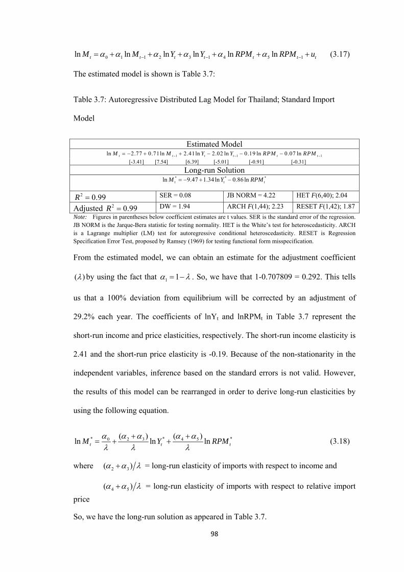
0 1 1 2 3 1 4 5 1ln ln ln ln ln lnt t t t t t tM M Y Y RPM RPM uα α α α α α− −= + + + + + +− (3.17)
The estimated model is shown is Table 3.7:
Table 3.7: Autoregressive Distributed Lag Model for Thailand; Standard Import
Model
Estimated Model 1 1ln 2.77 0.71ln 2.41ln 2.02 ln 0.19 ln 0.07 lnt t t t t 1tM M Y Y RPM RPM− − −= − + + − − −
[-3.41] [7.54] [6.39] [-5.01] [-0.91] [-0.31]
Long-run Solution * *ln 9.47 1.34 ln 0.86 lnt t
*tM Y R= − + − PM
2 0.99R = SER = 0.08 JB NORM = 4.22 HET F(6,40); 2.04
Adjusted 2 0.99R = DW = 1.94 ARCH F(1,44); 2.23 RESET F(1,42); 1.87 Note: Figures in parentheses below coefficient estimates are t values. SER is the standard error of the regression. JB NORM is the Jarque-Bera statistic for testing normality. HET is the White’s test for heteroscedasticity. ARCH is a Lagrange multiplier (LM) test for autoregressive conditional heteroscedasticity. RESET is Regression Specification Error Test, proposed by Ramsey (1969) for testing functional form misspecification.
From the estimated model, we can obtain an estimate for the adjustment coefficient
( )λ by using the fact that 1 1α λ= − . So, we have that 1-0.707809 = 0.292. This tells
us that a 100% deviation from equilibrium will be corrected by an adjustment of
29.2% each year. The coefficients of lnYt and lnRPMt in Table 3.7 represent the
short-run income and price elasticities, respectively. The short-run income elasticity is
2.41 and the short-run price elasticity is -0.19. Because of the non-stationarity in the
independent variables, inference based on the standard errors is not valid. However,
the results of this model can be rearranged in order to derive long-run elasticities by
using the following equation.
* *0 2 3 4 5( ) ( )ln ln lnt t*tM Y RPMα α α α α
λ λ λ+ +
= + + (3.18)
where 2 3( )α α λ+ = long-run elasticity of imports with respect to income and
4 5( )α α λ+ = long-run elasticity of imports with respect to relative import price
So, we have the long-run solution as appeared in Table 3.7.
98

We also estimate the autoregressive distributed lag model for augmented import
model which now includes Thailand’s average tariff rates as a liberalization measure.
Again, by using the Schwarz’s criterion, we find that the optimum lag using in the
estimation is (1,1). The estimated model is as follow and the estimated results are
reported in Table 3.8.
0 1 1 2 3 1 4 5 1
6 7 1
ln ln ln ln ln lnln lnt t t t t t
t t t
M M Y Y RPM RPMTT TT uα α α α α α
α α− − −
−
= + + + + ++ + +
(3.19)
Table 3.8: Autoregressive Distributed Lag Model for Thailand; Augmented Import
Model
Estimated Model 1 1 1ln 2.39 0.70ln 2.21ln 1.82ln 0.11ln 0.08ln 0.23ln 0.21lnt t t t t t t 1tM M Y Y RPM RPM TT TT− − −= − + + − − − − + −
[-2.75] [7.39] [5.81] [-4.58] [-0.53] [-0.40] [-2.51] [2.18]
Long-run Solution * * *ln 7.96 1.28 ln 0.64 ln 0.07 lnt t t
*tM Y RPM= − + − − TT
2 0.99R = SER = 0.08 JB NORM = 2.93 HET F(8,37); 1.69
Adjusted 2 0.99R = DW = 2.21 ARCH F(1,44); 2.75 RESET F(1,41); 1.12
Note: Figures in parentheses below coefficient estimates are t values. SER is the standard error of the regression. JB NORM is the Jarque-Bera statistic for testing normality. HET is the White’s test for heteroscedasticity. ARCH is a Lagrange multiplier (LM) test for autoregressive conditional heteroscedasticity. RESET is Regression Specification Error Test, proposed by Ramsey (1969) for testing functional form misspecification.
After estimating the model, we can obtain an estimate for the adjustment coefficient
( )λ which is equal to 0.30. In the augmented model, the short-run income elasticity is
2.21 and the short-run price elasticity is -0.11. The short-run elasticity of imports with
respect to tariff is -0.23. The long-run demand for import can be calculated as shown
above in Table 3.8.
4) Exogeneity; Import Demand Function
One of the conditions necessary to perform inference in a single-equation framework
is weak exogeneity of the cointegrating variables. Johansen (1992) shows that, under
weak exogeneity, single-equation estimation remains efficient in a cointegrated
99

system, whereas if weak exogeneity fails, then system modelling is needed despite the
super consistency of estimators in I(1) processes.11 In some cases, the failure of weak
exogeneity can lead to a large loss of efficiency.12 Thus, testing for weak exogeneity
is as important in non-stationary cointegrated systems as it is in stationary cases.13
According to Harbo, Johansen, Nielsen, and Rahbek (1998), weak exogeneity can be
tested by estimating the conditional model with assumed exogeneity and inserting the
estimated cointegrating vectors back into the marginal model. Weak exogeneity is
established by statistical insignificance of the cointegrating vectors in the marginal
model. More specifically, weak exogeneity of Thailand’s real income, relative import
price, and Thailand’s average tariff rates will be accepted if the error-correction term
of conditional model for import demand is statistically insignificant.
Therefore, we start by specify three autoregressive marginal models for domestic
income , relative import price ( ln )YΔ ( ln )RPMΔ , and Thailand’s average tariff rates
. In order to obtain well specified marginal processes, an appropriate dummy
variable is added into each model, including 1) in marginal model for ,
dum1997 for taking into account the Asian financial crisis in 1997; 2) in marginal
model for , dum1973 for taking into account the oil price shock in 1973
and; 3) in marginal model for
( lnTTΔ )
lnΔ
lnYΔ
RPM
lnTTΔ , dum1992 for taking into account the
membership of AFTA and the WTO membership which Thailand joined since 1992
and 1995, respectively. The value of the dummies is 1 for the observations indicated
by their names and 0 elsewhere. Then, we add the error-correction term
1 3 lnt t 1 5 ln 1t 7 1ln )t(ln M Y RPM TTα α α −+− −− + − into the marginal models of real
11 See Philips (1990), and Philips and Loretan (1991) for example. 12 See Hendry and Mizon (1991) for example. 13 See Ericsson (1992)
100

income, relative prices, and average tariff rates, and re-estimate them to investigate
the significance of the error-correction term. We also provide various diagnostic tests
and these tests uniformly suggest that, in all case, marginal models for ,
, and do not suffer from problems of non-normality, serial
correlation, heteroscedasticity, and mis-specification. The results are reported below:
lnYΔ
ln RPMΔ
lnYΔ =
2 0.39R =
lnTTΔ
lnYΔ
0.28 lnt tY+ Δ
Marginal model for augmented by the error-correction term
1 10.13 0.06 1997 0.04dum ecm− −− − − t [-1.84] [1.95] [-2.97] [-1.55]
0.03SER = 1.82DW =
; 0= .73NORM JB ; (1, 43) 2.54ARCH F = ; (5, 40) 0.79HET F =
; (RESET F
ln
1, 41) = 0.20
lnΔ
0.35
Marginal model for augmented by the error-correction term RPM
RPM 1 10.20 ln 0.15 1973 0.04t t tRPM dum ecm− −Δ = Δ + − − + [-1.79] [2.92] [3.86] [-1.45]
0.05SER = 1.92DW = 2 0.38R =
; 0= .78NORM JB ; (1, 43) 2.57ARCH F = ; (5, 40) 0.HET F = 68
; (RESET F
lnTTΔ =
2 0.39R =
1, 41) = 0.09
lnTTΔ
0.33 lnTT− Δ
Marginal model for augmented by the error-correction term
1 10.26 0.45 1992 0.06t t dum ecm− −− + t [1.92] [-2.47] [-5.16] [1.04]
0.11SER = 1.95DW =
; 1= .16NORM JB ; (1, 43) 0.16ARCH F = ; (5, 40) 0.HET F = 51
; (RESET F 1, 41) = 0.24
It is clear from the results that the coefficient of the error-correction term is
insignificant for all three models, confirming that Thailand’s real GDP, relative
101

import price, and Thailand’s average tariff rates can be considered as weakly
exogenous.
5) Dynamic Adjustment Estimates
In this section, we determine how well the dynamic process which generates
Thailand’s level of imports can be captured by a single-equation error-correction
model (SEECM). From results presented above, the presence of a cointegrating vector
together with the evidence of weak exogeneity suggest that we can use a single-
equation error-correction representation without the loss of either efficiency or the
ability to perform proper inference.14 From our general ARDL model;
Standard Import Model:
0 1 20 0 0
ln ln ln lnp q q
t i t i i t i i t i ti i i
M Y RPM uα α α α− − −= = =
= + + + +∑ ∑ ∑
i t
M
and Augmented Import Model:
0 1 2 30 0 0 0
ln ln ln ln lnp q q q
t i t i i t i i t i i ti i i i
M M Y RPM TT uα α α α α− − −= = = =
= + + + + +∑ ∑ ∑ ∑ −
1t
By differencing the ARDL model and rewriting ARDL to ECM, a re-parameterization
of the ARDL equation in the form of an error-correction model (SEECM) can be
written as;
Standard Import Model:
*1 1ln ( ) ln ( ) ln ( ) ln [ln ln ]t t i t t t tM A L M B L Y C L RPM M Mϕ μ− −Δ = Δ + Δ + Δ + − +−
and Augmented Import Model:
14 See Banerjee et al. (1986, 1993)
102
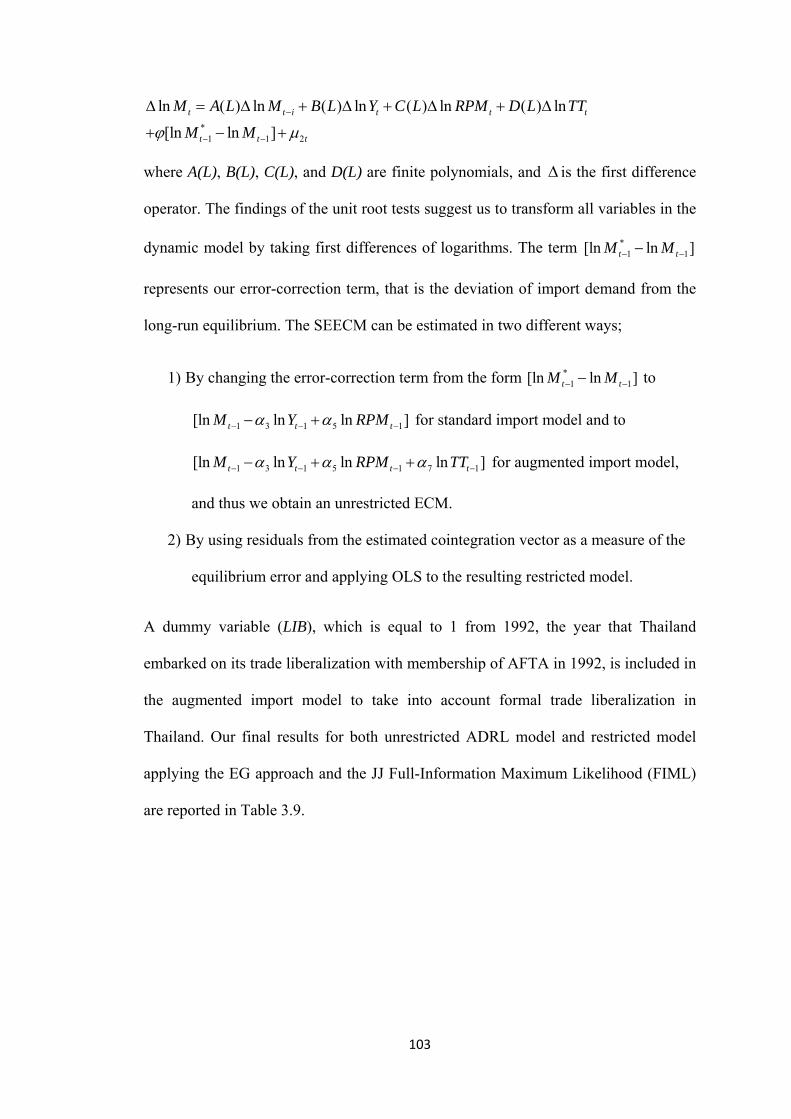
*1 1 2
ln ( ) ln ( ) ln ( ) ln ( ) ln
[ln ln ]t t i t t
t t t
tM A L M B L Y C L RPM D L T
M Mϕ μ−
− −
Δ = Δ + Δ + Δ + Δ
+ − +
T
where A(L), B(L), C(L), and D(L) are finite polynomials, and Δ is the first difference
operator. The findings of the unit root tests suggest us to transform all variables in the
dynamic model by taking first differences of logarithms. The term *1 1[ln ln ]t tM M− −−
or-correction term, that is the deviation of import demand from the
long-run equilibrium. The SEECM can be estimated in two different ways;
represents our err
1) By changing the error-correction term from the form to *1 1[ln ln ]t tM M− −−
1 3 1 5 1[ln ln ln ]t t tM Y RPMα α− − −− + for standard impo
7 1ln ]t
rt model and to
1 3 1 5 1[ln ln lnt t tM Y RPM TTα α− − α −−− + + for augmented import
y using residuals from the estimated coint
model,
and thus we obtain an unrestricted ECM.
2) B egration vector as a measure of the
A dummy variable (
equilibrium error and applying OLS to the resulting restricted model.
LIB), which is equal to 1 from 1992, the year that Thailand
embarked on its trade liberalization with membership of AFTA in 1992, is included in
the augmented import model to take into account formal trade liberalization in
Thailand. Our final results for both unrestricted ADRL model and restricted model
applying the EG approach and the JJ Full-Information Maximum Likelihood (FIML)
are reported in Table 3.9.
103

ln MΔTable 3.9: Error-Correction Model for Import Demand ( )
el Augmented Model (dummy)
Variable Standard Model Augmented Mod
Unrestricted Restricted Restricted JJ
Unrestricted Restricted Restricted Unrestricted Restricted Restricted EG EG JJ EG JJ
ln tY Δ 2.41**(0.38)
*** 7)
2.21(0.38)
*
2.35(0.41)
*
* 2.26*** (0.36)
2.31(0.3
***
2.15*** (0.33)
2.13**(0.36)
***
2.37*** (0.39)
2.25**(0.42)
ln tRPMΔ -0.19 (0.21)
-0.10 (0.20)
-0.21 (0.22)
-0.11 (0.20)
-0.08 (0.18)
-0.15 (0.21)
-0.09 (0.20)
-0.12 (0.19)
-0.17 (0.21)
lnTTΔ t -0.23***
(0.09) -0.26*** (0.09)
-0.22** (0.09)
-0.19* (0.10)
-0.22** (0.09)
-0.20* (0.10)
1tecm − -0.30*** ** ** * * (0.09)
-0.31*(0.12)
-0.30*(0.09)
-0.28*(0.11)
-0.32***(0.09)
-0.28*(0.11)
1ln tM − -0.29*** (0.09)
* -0.30*** (0.09)
-0.34**(0.10)
1ln tY − 0.39*** (0.12)
39*** (0.12)
42*** (0.12)
0. 0.
1ln tRPM − -0.25** (0.10)
-0.19* (0.10)
-0.17* (0.10)
1ln tTT − -0.02 (0.05)
-0.01 (0.05)
tLIB 0.06 (0.06)
0.03 (0.02)
02 (0.03) 0.
Constant .77*** (0.81)
.06** (0.03)
.06*** (0.03)
** .06*** (0.02)
.06** (0.03)
** .09*** (0.03)
.07** (0.03)
-2 -0 -0 -2.39*(0.87)
-0 -0 -2.31*(0.87)
-0 -0
2R 0.59 57 54 0.65 64 0.60 0. 0. 0. 0.65 0.65 0.60
2R 0.54 0.54 0.51 0.58 0.60 0.56 0.58 0.60 0.55
SER 0.08 0.08 0.08 0.08 0.08 0.08 0.08 0.08 0.08
DW 1.94 1.84 2.34 2.22 2.17 2.25 2.18 2.18 2.16
NORM JB = 1.14 JB = JB = JB = 2.93 JB = JB = JB = 2.53 JB = JB = 1.22 2.00 2.16 0.01 2.28 0.10
ARCH F(1,44) =3.18
F(1,44) = 2.07
F(1,42) = 3.34
F(1,44) =2.75
F(1,44) = 2.31
F(1,42) = 1.75
F(1,44) =2.19
F(1,44) = 2.37
F(1,42) = 1.58
HET F(10,36) = 2.10
F(6,40= 1.89
)
)
)
)
)
)
F(6,38= 0.80
F(14,32) = 3.93
F(8,38= 3.14
F(8,36= 1.05
F(15,31) = 3.63
F(9,37= 2.45
F(9,35= 1.01
RESET F(1,40) = 0.61
F(1,42) = 0.71
F(1,40) = 0.45
F(1,38) = 0.44
F(1,41) = 1.04
F(1,39) = 0.01
F(1,37) = 0.45
F(1,40) = 1.16
F(1,38) = 0.01
Note: he aster ( in tat i t , 5 an respect ely. Figures in rent w ent es rd
by Ramsey (1969) for testing
similar. Although we interpret our results based on comparison purpose, we focus our
2
higher than those of the general unrestricted autoregressive model (in fact, SER of the
Tiv
isks (***), **), (*) dicate s istical sign ficance a the 10% %, and 1% signific ce level,
pa heses belo coeffici estimat are standa errors. SER is the standard error of the regression. DW is the Durbin-Watson Statistic. NORM is the Jarque-Bera statistic for testing normality. ARCH is the test for autoregressive conditional heteroscedasticity. HET is the White’s test for heteroscedasticity. RESET is Regression Specification Error Test, proposedfunctional form misspecification.
From Table 3.9, the results of the two models (unrestricted and restricted) are very
economic interpretation on the restricted SEECM using EG approach, since this
model is more preferable on the ground of goodness-of-fit criteria. First, considering
both the standard and augmented import model, the R value can be considered good
(0.59 to 0.65). The estimated standard error of regression, in all cases (0.08) are not
restricted model is slightly lower than that of unrestricted model when working to a
104

number of decimal places), suggesting the validity of the parameter-reduction process.
All the diagnostic tests confirm the appropriateness of the specification which suggest
to us that all import demand models are appropriately set.
In both standard and augmented models, the coefficient of the error-correction term,
which reflects the impact of having 1ln tM − out of the long-run equilibrium, appears
highly significant at 1% level and e correct (negative) sign, suggesting the
significance of the speed of adjustment in response to a deviation from the long run
equilibrium. The error-correction coefficient of standard model, estimated at -0.30, is
almost equal to that of augmented models (-0.32 for augmented model with dummy).
This shows a slow speed of convergence to equilibrium, which is accounted
approximately 30% each year.
Next, considering the short-run incom
has th
e elasticity, this estimate for both the standard
coefficient of the
and the augmented models is larger than the long-run elasticity (+2.26 for standard
model, +2.15 for augmented model without liberalization dummy, and +2.37 for
augmented with liberalization dummy), suggesting that the income change has a
potentially comtemporaneous effect on the change of the volume of imports. The size
of the coefficients shows a large and immediate impact of a change in GDP on import
demand. However, the price elasticity does not appear to be significant in the short-
run, though it is significant in the long run and has an expected sign.
Considering the measures of trade liberalization, on one hand, the
average tariff rates is significant with an expected sign, implying that the effect of
change in tariff rates on the volume of imports is negative. The estimated coefficient
indicates that a 1 percent change in tariff rates leads to approximately 0.2 percent
change in the level of imports. It is also found that the short-run elasticity is larger
105

than that of the long run. On the other hand, trade liberalization dummy appears to be
insignificant both in standard and augmented models.
The insignificance of relative import price elasticity must be carefully taken care of.
import to export demand. Again, we first
As mentioned in Carone (1996), this may be due to the measurement errors in the data
coming from the method of calculation of our import price, in which we use the
import unit value index as a proxy for import price. Carone (1996) has suggested that
it could possibly lead the estimated coefficient to be biased toward zero. Another
explanation is on the downward bias which could possibly have arisen from the use of
a domestic price index. This is because this index is composed of both tradable and
non-tradable goods. However, these two indices are the only close approximations for
the calculation of relative import prices now available over a long period of time.
3.5.2. Export Demand
3.5.2.1. The Analysis of the Long-run Total Export Demand
1) Stationary Test: Unit Root Analysis
Now, we turn our investigation from
conduct tests for the time series properties of the variables concerned. Like for import
demand, we employ standard unit root tests by applying two asymptotically
equivalent tests: the augmented Dickey-Fuller (ADF) test and the Phillips-Perron (PP)
test. Our observed time series include aggregate export volume ( )X , world GDP ( )W
, relative export price ( / )RPX PX PW= , and world’s average tariff rates ( )TW . All
rithms. The results from these tests for
each variable are provided in the table below and can be seen that the ADF and PP
variables have been converted to natural loga
tests suggest non-stationarity of each variable when expressed in levels.
106

Table 3.10: ADF and PP Unit Root Tests for Stationarity (Export Model)
Test for I(0) Test for I(1) ln(X) ln(W) ln(RPX) ln(TW) Δln(X) Δln(W) Δln(RPX) Δln(TW)
ADF without trend -0.59 -2.49 -2.01 0.60 -6.81 -3.73 -6.72 -5.69 with trend -1.60 -3.05 -2.22 -1.39 -6.73 -4.39 -6.71 -5.58
PP without trend -0.59 -2. 1.04 -6.81 -3.6 -5.62 51 -1.90 6 -8.70with trend -1.65 -2.89 -2.21 -1.42 -6.73 -4.29 -11.06 -5.76
e th ts te t the variables under consideration are
ationary in their first differences. From the results we conclude that the variables are
ined that the examined variables are integrated of order 1,
erformed. First, the cointegration test using the two-step
estimation, suggested by Engle and Granger, is employed. The results of the OLS
ln 19.24 1.82ln 0.52lnt t t
From Tabl 3.10, e tes indica hat
st
integrated of order 1.
2) Cointegration Analysis
Since it has been determ
cointegration analysis is p
regression are shown below:
Standard Export Model
X W RPX= − + − (3.20)
] [-5.24]
R2 = 0.99 SER = 0.10 DW = 0.96
Cointegration Tests
CRDW; 0.511, 0.386, 0.322 (1, 5 and 10 percent critical values)
ADF = -2.72 [-1.95] PP = -2.72 [-1.95]
From the cointegrating equation shown above, an economic interpretation of the
results can be presented as follows; the long-run income elasticity of demand for
exports is high (one percent increase in world’s GDP increases exports by 1.82
[-18.99] [32.26
107

percent), while the long-run price elasticity of demand for exports is rather low (one
percent decrease in relative export price increases exports by only 0.52 percent).
I(0). If it appears that the residuals obtained in the first step is stationary, they can be
included as error-correction term in the estimation of the short-run dynami
In the second step, we test whether the residuals obtained from equation (3.20) are
cs of
Next, we perform the Cointegrating Regression Durbin-Watson (CRDW) test as
equation (3.20) is 0.96 which is greater than
exports in ECM model. First, we employ the ADF test to check the stationary of
residuals. The result shows that the t-statistic is -2.72, while the 95% critical value for
the test is -1.95. We are then inclined to reject the null hypothesis of a unit root in the
residuals at the 5% significance level. The PP test also supports the result obtained
from the ADF test. The test statistic is equal to -2.72, which is greater than the PP (-
1.95) at 5% critical level. Both results obtained from the ADF and PP tests infer about
cointegration between variables.
Gujarati (2003) suggested. The null hypothesis is that there is a unit root in the
residuals. The DW statistic obtained from
the critical values (0.511, 0.386, 0.322 for 1%, 5% and 10% levels of significance
respectively), and thus we can reject the hypothesis that the residuals are non-
stationary and confirm the hypothesis of cointegration.
Now, we include world’s average tariff rate as our liberalization measure. The results
are presented as follows;
108

Augmented Import Model
t5.99 1.31ln 0.20ln 0.62lnt t tX W RPX= − + − −ln TW (3.21)
[-2.28] [-6.20]
R2 = 0.99 SER = 0.10 DW = 1.14
Cointegration Tests
itical values)
-1.95]
ce elasticities in augmented export model are lower than those
er than unity (1.31),
ice elasticity is quite low (-0.20). Exports moderately respond to
95% critical value (-1.95). Likewise, the t statistic obtained from the PP test is -2.98,
rated. Before carrying out the
cointegration test, we first specify the relevant order of lags (p) of the Vector
[-2.64] [14.16]
CRDW; 0.511, 0.386, 0.322 (1, 5 and 10 percent cr
ADF = -2.98 [-1.95] PP = -2.98 [
The income and pri
found in standard model. The long-run income elasticity is high
while the long-run pr
changes in the world’s average tariff rate since a one percent decrease in world’s
average tariff rate is associated with only 0.62 percent increase in exports.
We then perform the unit root test for the series of residuals obtained from equation
(3.21). The ADF test shows that the t-statistic is -2.98, which is over than the ADF
lower than the PP (-1.95) at 5% critical level. The CRDW test also points out in the
same way. The DW statistic obtained from equation (3.21) is 1.14 which is greater
than the critical values (0.511, 0.386, 0.322 for 1%, 5% and 10% levels of
significance respectively). Thus, we can then reject the null hypothesis of a unit root
in the residuals at the 5% significance level and it can be concluded that there is
cointegration between variables.
Next, the cointegration test using the JJ method is undertaken to determine whether
any combinations of the variables are cointeg
109

Autoregression (VAR) model. The lag order is determined using the Schwarz
criterion. By doing this, we find that the optimum lag length is equal to 1.
According to Johansen and Juselius (1990), there are two tests for the number of
cointegrating relations; the maximum eigenvalue and the trace test. Table 3.11 an
After the optimum lag length is found, we now can perform the cointegration test.
d
Tests
3.13 report the results of these tests for cointegrating relationship between variables.
The results indicate that there exists only one cointegrating relationship, both for the
standard and the augmented export models and the cointegration vectors are presented
in Table 3.12 and 3.14, respectively.
Table 3.11: Johansen Tests for the Number of Cointegrating Vectors: Standard Export
Model
Maximal eigenvalues Eigenvalue Trace Null Alternative Statistics 95% critical
value Statistics 95% critical
value 0 29.84 21.13 42.16 29.80 r = 1r = 1r ≤ 2r = 10.41 14.26 12.32 15.49 2r ≤ 3r = 0.04 1.91 1.91 3.84
Note: denotes the numb of cointegrati
Table 3.12: Cointegration Vector: S
Coi n vec
r er ng vectors.
tandard Export Model
ntegratio tor: ln(X) ) ln(W ln(RPX) -1.00 1.77 -0.52
[4.77] [-2.81] Note: t ratio is shown in parentheses [ ]
110

Table 3.13: Johansen Tests for the Number of Cointegrating Vectors: Augmented
Export Model by Including the World’s Average Tariff Rates
Tests Maximal eigenvalues Eigenvalue Trace
Null Alternative Statistics 95% critical tics 95% critical value
Statisvalue
0r = 1r = 36.61 27.58 59.59 47.86 1r ≤ 2r = 13.88 21.13 22.98 29.80 2r ≤ 3r = 8.67 14.26 9.11 15.49 3r ≤ 4r = 0.44 3.84 0.43 3.84
Note: r denotes the number of cointegratin
Table 3.14: Cointegration Vector: Augmented rt Model cluding ’s
tion vector:
g vectors.
Expo by In World
Average Tariff Rates
Cointegraln(X) ln(W) ln(RPX) ln(TW) -1.00 1.34 -0.27 -0.71
[4.76] [-2.42] [-3.78] Note: s shown in p s [ ]
cien ted obtained from the JJ method are very
timate a dynamic relationship for
of a unique long-run relationship. Thus we can now proceed to the estimation of the
t ratio i arenthese
Again, it is found that the coeffi ts estima
similar to those obtained from the two-step EG method.
3) Autoregressive Distributed Lag (ARDL) Model
In this section, we use the ARDL approach to es
Thailand’s export demand over the period 1960-2007. In the export model, the
volume of exports is explained by lags of itself and the current and lagged values of a
number of explanatory variables (world income, relative export prices, world tariffs),
and hence the ADRL model has an appealing separation of short- and long-run
effects. As shown above, the ADF and PP tests confirm that the I(1) hypothesis
cannot be rejected for each variable at the 5% level of significance. Then, the JJ test
for the number of cointegrating relationships among variables indicates the presence
111

ARDL model. In estimating the Autoregressive Distributed Lag Model for Thailand’s
Import Demand, we pick the lag-lengths (p,q) using Schwarz’s criterion. This results
in lag length equal to (1,1) which is reasonable since we are dealing with annual data.
Thus, the ARDL model for Thailand’s import demand can be presented as follow;
0 1 1 2 3 1 4 5 1ln ln ln ln ln lnt t t t t t tX X W W RPX RPX uβ β β β β β− −= + + + + + +− (3.22)
The estimated model is shown is Table 3.15:
Table 3.15: Autoregressive Distributed Lag Model for Thailand; Standard Export
Estimated Model
Model
1 1ln 3.82 0.80 ln 0.75 ln 0.39 ln 0.19 ln 0.09 lnt t t t t 1tX X W W RPX RPX− − −= − + + − − + [-2.20] [9.58] [2.45] [-1.18] [-1.82] [0.81]
Long-run Solution * *ln 1 lnt t
*t9.52 1.85 ln 0.55X W+ − R= − PX
2 0.99R = SER = 0.07 JB NORM = 1.75 HET F(10,36); 0.48
Adjusted DW = 2. (1,44); 0.71 RESET F(1,40); 3.24 2 0.99R = 16 ARCH F
From the estimated model, we can obtain an dj estimate for the a ustment coefficient
( ) by using the fact that 1 1β λ= −λ . So, we have that 1-0.804 = 0.196. This tells us
eac of lnXt
that a 100% deviation from equilibrium will be corrected by an adjustment of 19.6%
h year. The coefficients and lnRPXt in Table 3.15 represent the short-run
income and price elasticities, respectively. The short-run income elasticity is 0.75 and
the short-run price elasticity is -0.19. Because of the non-stationarity in the
independent variables, inference based on the standard errors is not valid. However,
the results of this model can be rearranged in order to derive long-run elasticities by
using the following equation.
* *0 2 3 4 5( ) ( )ln ln ln *tt tX W RPXβ β β β β
λ λ+ +
= + +λ
(3.23)
112
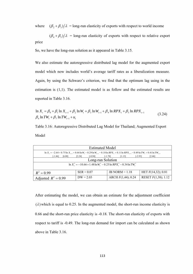
where 2 3( )β β λ+ = long-run elasticity of exp
orts with respect to world income
4 5( )β β λ+ = long-run elasticity of exports with respect to relative export
the augmented export
model which now includes world’s average tariff rates as a liberalization measure.
Again, by using the Schwarz’s criterion, we find that the optimum lag using in the
estimation is (1,1). The estimated model is as follow and the estimated results are
reported in Table 3.16.
1t
price
So, we have the long-run solution as it appeared in Table 3.15.
We also estimate the autoregressive distributed lag model for
0 1 1ln lnt t 2 3 1 4 5
6 7 1
ln ln ln lnln ln
t t t
t t t
X X W W RPX RPTW TW u
Xβ β −= + + β β β ββ β
−
−
+ + ++ +
− (3.24)
Table 3.16: Autoregressive Distributed Lag Model for Thailand; Augm
Model
Estimated Model
ented Export
1 1 1ln 2.64 0.75 ln 0.66 ln 0.29 ln 0.18 ln 0.11ln 0.49 ln 0.41lnt t t t t t t 1tX X W W RPX RPX TW TW− − −= − + + − − + − + −
[-1.46] [6.88] [2.24] [-0.94] [-1.78] [1.13] [-2.93] [2.46]
Long-run Solution * * *ln 10.66 1.48 ln 0.25 ln 0.34 lnt t t
*tX W RPX TW= − + − −
2 SER = RM = 1.18 HET F(14,32)0.99R = 0.07 JB NO ; 0.81
Adjusted DW = 2.03 ARCH F(1,44); 0.24 RESET F(1,38); 1.12 2 0.99R =
After estimating the model, we can obtain an estimate for the adjustment coefficient
( )λ which is equal to 0.25. In the augmented model, the short-run income elasticity is
0.66 and the short-run price elasticity is -0.18. The short-run elasticity of exports with
respect to tariff is -0.49. The long-run demand for import can be calculated as shown
above in Table 3.16.
113

4) Exogeneity; Expo nd Function
ee autoregressive marginal models for the
rt Dema
Δ
Following the same step, we specify thr
world’s real income ( ln )W , relative export prices ( ln )RPXΔ , and world’s average
tariff rate ( ln )TWΔ . We include a dummy variable arginal model and the
detail is as f ) in marginal model for lnW
for each m
ollows; 1 Δ , dumREC for taking into account
the world economic recession resulting from , when world economic
growth was weak between 1973-1975; 2) in marginal model for ln RPXΔ , dum1973
for taking into account the oil price shock in 1973 and; 3) in m odel for
lnTWΔ , dumGATT for taking into account the two phases of GATT including
The error-correction term
1 3 1 5 1 7 1(ln ln ln ln )t t t tX W RPX TW
the oil crisis
arginal m
Tokyo Round and Uruguay Round.15
β β β− − − −− + + is again added into the marginal
mode and world’s average tariff rate, and
each model is re-estimated in order to investigate the significance of the error-
correction term. The test results are listed below;
Marginal model for lnWΔ augmented by the erro
ls of world real income, relative export price,
r-correction term
[-1.18] [3.86] [-1.85) [-1.33] 1 1ln 0.13 0.51 0.01 0.01t t tW dumREC ecm− −Δ = − + − − lnWΔ
2 0.35R = 0.01SER = 1.95DW =
; 0.0NORM JB = 2 ; (1, 43) 0.01ARCH F = ; (5, 40) 1.72HET F =
; (1, 41) 0.05RESET F =
15 Tokyo Round is the final round in the second phase, starting from 1973 and covering for 74 months. This round focuses on the reduction tariff barriers. This round is considered as a major tariff reduction round since tariffs worth more than 300 billion US dollars were reduced between 1973 and 1979. The third phase of GATT consists only of Uruguay Round which starts from 1986 to 1994. In this round, not only tariffs were continually reduced, but new areas such as textiles, clothing, and agricultural products were also included in trade negotiations. Intellectual property rights were also considered. After this round, the GATT becomes the WTO in 1995.
114

Marginal model for augmented by the error-correction term
t
ln RPXΔ
1 1ln 1.14 0.45 ln 0.30 1973 0.11t tRPX RPX dum ecm− −Δ = − Δ + − [1.68] [-2.45] [6.65] [-1.41]
2 0.50R = 0.05SER = 1.83DW =
; 0.5NORM JB = 6 ; (1, 42) 0.14ARCH F = ; (5,39) 0.75HET F =
; (1,39) 0.08RESET F =
Marginal model for augmented by the error-correction term
t
lnTWΔ
1 1ln 0.59 0.56 ln 0.58 0.05t tTW TW dumGATT ecm− −Δ = − − Δ − − [-0.40] [-4.36] [-5.81] [-0.38]
2 0.45R = 0.11SER = 1.88DW =
; 0.NORM JB = 41 ; (1, 42) 0.23ARCH F = ; (5,39) 0.74HET F =
; (1,39) 0.39RESET F =
The results presenting above show that, for all marginal models, the coefficient on the
error-correction term is insignificant. This is a strong evidence of weak exogeneity.
Therefore, we can conclude that lnWΔ , ln RPXΔ , and lnTWΔ are weakly
exogenous and it is possible to condition the short-run model on these variables.
5) Dynamic Adjustment Estimates
In this section, we determine how well the dynamic process which generates
Thailand’s volume of exports can be captured by a single-equation error-correction
together with the evidence of weak exogeneity suggest that we can construct a single-
model (SEECM). From results presented above, the presence of a cointegrating vector
equation error-correction model. From our general ARDL model;
115
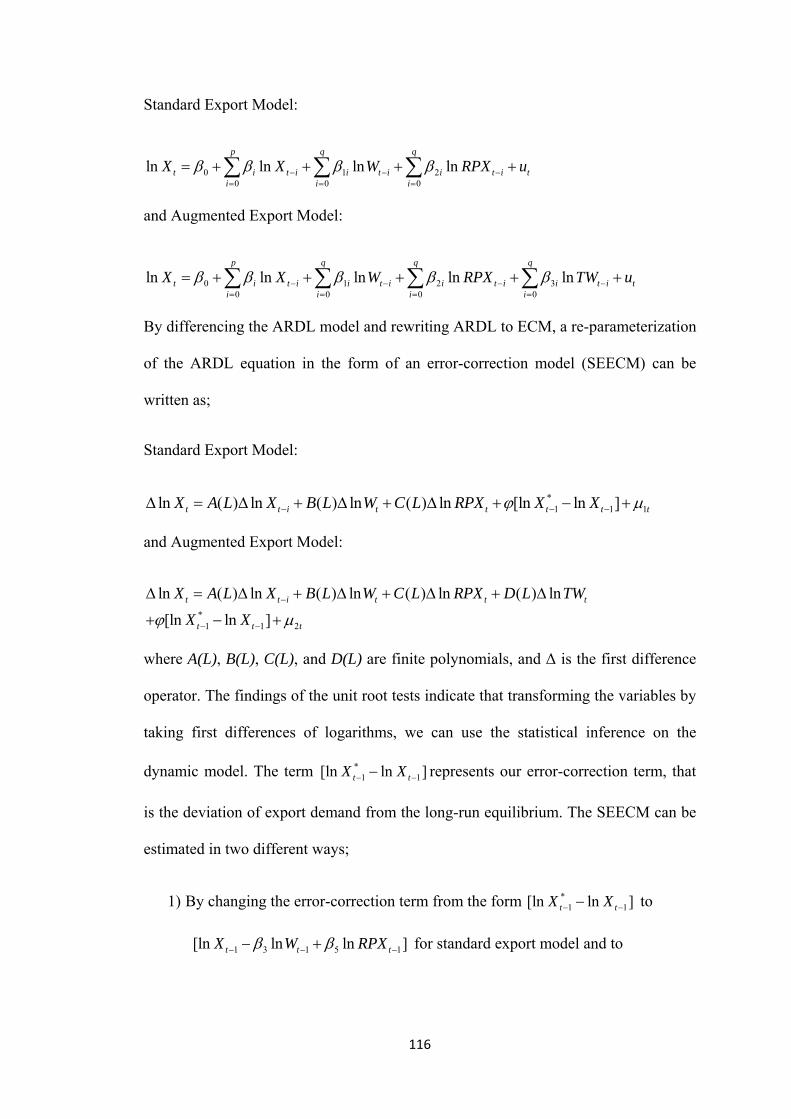
Standard Export Model:
0 1 20 0 0
ln ln ln lnp q q
t i t i i t i i t i ti i i
X X W RPXβ β β β− −= = =
= + + + +∑ ∑ ∑ u−
and Augmented Export Model:
0 1 2 30 0 0 0
ln ln ln ln lnp q q q
t i t i i t i i t i i t i ti i i i
X X W RPX TW uβ β β β β− − −= = = =
= + + + + +∑ ∑ ∑ ∑ −
l and rewriting ARDL to ECM, a re-parameterization
of the ARDL equation in the form of an error-correction model (SEECM) can be
written as;
1t
By differencing the ARDL mode
Standard Export Model:
ln tX A *1 1( ) ln ( ) ln ( ) ln [ln ln ]t i t t t tL X B L W C L RPX X Xϕ μ− −Δ + Δ + Δ + − + Δ = −
odel:
t
and Augmented Export M
*1 1 2
ln ( ) ln ( ) ln ( ) ln ( ) ln
[ln ln ]t t i t t
t t t
X A L X B L W C L RPX D L TW
X Xϕ μ−
− −
Δ = Δ + Δ + Δ + Δ
+ − +
where A(L), B(L), C(L), and D(L) are finite polynomials, and Δ is the first difference
operator. The findings of the unit root tests indicate that transforming the variables by
taking first differences of logarithms, we can use the statistical inference on the
dynamic model. The term *1 1[ln ln ]t tX X− −− represents our error-correction term, that
1) By changing the error-correction term from the form 1 1[ln ln ]t tX X− −− to
1 3 1 5[ln ln lnt tX W
is the deviation of export demand from the long-run equilibrium. The SEECM can be
estimated in two different ways;
t
*
1]RPXβ β− − −− + for standard export model and to
116

1 3 1 5 1 7 1[ln ln ln ln ]t t t tX W RPX TWβ β β− − − −− + + for au mod
ECM.
tion vector as a measure of the
equilibrium error and applying OLS to the resulting restricted m
gmented export el,
2)
odel.
A d
the libe gmented
and thus we obtain an unrestricted
By using residuals from the estimated cointegra
ummy variable (LIB), which is equal to 1 from 1992, the year that Thailand started
ralization process with membership of AFTA, is included in the au
export model to take into account formal trade liberalization in Thailand. Our final
results for both unrestricted ADRL model and restricted model applying JJ Full-
Information Maximum Likelihood (FIML) are reported in Table 3.17.
Table 3.17: Error-Correction Model for Export Demand ( ln XΔ )
Variable Standard Model Augmented Model Augmented Model (dummy)
Unrestricted Restricted EG
Restricted JJ
Unrestricted Restricted EG
Restricted JJ
Unrestricted Restricted EG
Restricted JJ
ln tWΔ 0.75** (0.31)
0.73*** (0.29)
0.65** (0.29)
0.66** (0.29)
0.71*** (0.27)
0.57** (0.27)
0.58* (0.32)
0.55*** (0.16)
0.45* (0.25)
ln tRPXΔ -0.19* (0.11)
5* 8)
-0.18*(0.10
-0.18*(0.10
-0.19* (0.10)
-0.1(0.0
)
-0.18** (0.09)
-0.14*(0.07)
)
-0.18* (0.09)
-0.14*(0.08)
ln tTWΔ -0.49*** -0.52*** -0.43*** -0.51*** -0.46*** (0.17) (0.15) (0.15) (0.17)
-0.55*** (0.16) (0.16)
1tecm − -0. -0.1 -0. -0.1 -0. -0.120**(0.08)
5* (0.07)
26**(0.11)
4* (0.07)
24**(0.11)
3* (0.07)
1ln tX − -0.20** (0.08)
-0.25**(0.11)
-0.23* (0.12)
1ln tW − 0.36** (0.16)
0.37** (0.16)
-0.10 (0.11)
1ln tRPX − -0.11 7)
.07) .07) (0.0
-0.06 (0
-0.06 (0
1ln tTW − -0.09 -0.10 (0.11)
(0.11)
tLIB 0.02 2)
0.02 .02)
0.03 (0.05) (0.0 (0
Constant 0.06*** .02)
0.06*** .02)
0.04** .02)
0.05** .02)
0.05** 2)
0.06*** .02)
-3.82**(1.74) (0 (0
-2.64* (1.50) (0 (0
-2.36* (1.37) (0.0 (0
2R 0.22 0.22 0.19 0.34 0.31 0.35 0.33 0.36 0.37
2R 0.13 17 0.13 28 25 28 24 0. 0.25 0. 0. 0.23 0. 0.
SER 0.07 07 0.07 0.07 06 07 0. 0. 0. 0.07 0.06 0.07
DW 2.16 2.15 2.19 2.03 1.98 2.18 2.09 2.03 2.19
NORM JB = 1.75 JB = 2.04
JB = 2.62
JB = 1.18 JB = 1.18
JB = 2.46
JB = 1.18 JB = 1.60
JB = 3.19
ARCH F(1,440.71
) = )
)
) = )
)
) = )
)
F(1,44= 0.69
F(1,44= 0.16
F(1,440.24
F(1,44= 0.26
F(1,44= 0.03
F(1,440.26
F(1,44= 0.06
F(1,44= 0.01
HET F(10,36) = )
)
) = )
)
) = )
) 0.45
F(6,40= 0.53
F(6,40= 0.69
F(14,320.62
F(8,38= 1.12
F(8,38= 1.51
F(15,310.73
F(9,37= 1.35
F(9,37= 1.66
RESET F(1,40) = )
)
) = )
)
) = )
) 1.36
F(1,42= 1.18
F(1,42= 2.73
F(1,380.14
F(1,41= 0.10
F(1,41= 2.06
F(1,370.25
F(1,40= 0.01
F(1,40= 1.49
117

As re orted le , ho m t u e m
unrestricted rest ) ery ilar. However, when considering both the
standard and augmented export model, the R2 values appear to be somewhat lower
than those of import models (0.19 to 0.37). The estimated standard errors for the
augmented models, in all cases, are lower general unrestricted
autoregressive model, suggesting the validity of the parameter-reduction process. All
the diagnostic tests confirm no evidence of high correlation, no serial correlation, no
any problem of heteroskedasticity, and no problem of non-normality in the residuals.
for both standard and augmented models, which indicate a slow speed of adjustment
towards the equilibrium state. The coefficients on the error-correction term can be
interpreted as the yearly speed of adjustment respect to short-run disequilibria. We
can read the estimated coefficient as if approximately 20-26% of any disequilibrium
inherited from the last period is eliminated in the next period.
and augmented models
are lower than unity (+0.73 for standard model, +0.71 for augmented model without
liberalization dummy, and +0.55 for augmented with liberalization dummy),
suggesting that world income change has a small immediate impact on change in the
volume of exports. However, the income impact seems to be larger in the long run
than in the short run.
n export price elasticity is negatively significant, showing an
p in Tab 3.17 like t se of i ports, he res lts of th two odels
( and ricted are v sim
than those of the
The estimated coefficient of error-correction term has a negative sign which is
consistent with the theory. However, the estimated values of the parameters are low
Considering the short-run income elasticity, the coefficients, in all cases, are
significant with correct sign. The estimates for both standard
For the short-run price elasticity, while the import price elasticity is insignificant in
short run, the short-ru
118

immediate effect on export demand. However, the values are all approximately equal
to 0.2, which indicate a low short-run inelastic response of the quantity of exports to
relative export price change.
The short-run elasticities of the world’s average tariff rate are -0.52 and -0.55. The
estimates are highly significant and have a negative sign as expected. This implies
We have used a battery of tests, and utilized all possible variants of estimation
run, in analyzing both the import demand
that world trade liberalization has an immediate impact on export demand. However,
the trade liberalization dummy appears to be insignificant, implying that trade
liberalization in Thailand (as becoming a member of AFTA and the WTO) does not
have any significant impact on export demand in the short run.
3.5.3. Comparison
methods for both the short run and the long
as well as the export demand function for Thailand. The reason for employing so
many tests, and considering both standard and non-standard estimation methods, is to
check on the robustness of the results. Since policy makers wish to re-structure policy
(trade liberalization or tariff reduction or alleviation of the trade deficit or currency
alignments), on the basis of the import and export demand functions, it is vital that we
get consistent, sensitive and robust results. Thus, we need to analyse carefully what
the estimated elasticities are and what implications they may have on trade policy.
However, simply because of the plethora of results, the variety of consistent estimates
used, and the many different parameter values of the estimated equations, it is
imperative to do a comparison and draw appropriate conclusion about the nature and
range of price/income elasticities in a small and highly open developing economy like
Thailand. In the following table, the empirical findings as for elasticities are summed
119

up and then these values are discussed carefully later. In what follows, we summarise
the results in tabular form and then conduct a comparative discussion drawing
conclusions on the policy implications of our results.
Table 3.18: Short-Run and Long-Run Elasticities
Imports Exports Thailand’s
GDP Relative
Import Price Thailand’s
Average Tariff Rate
World’s GDP Relative Export Price
World’s Average Tariff
Rate Short
Run Long Run
Short Run
Long Run
Short Run
Long Run
Short Run
Long Run
Short Run
Long Run
Short Run
Long Run
Long Run )
1.22 0.17 1.31 0.62 OLS (EG
-0.39 - -0.20 -
Cointegrating Vector (JJ)
1.25 1.34 -0.50 -0.18 -0.27 -0.71
ARDL(1,1) 2.21 1.28 -0.11 -0.64 -0.23 -0.07 0.66 1.48 -0.18 -0.25 -0.49 -0.34 Unrestricted ECM
2.21 -0.11 -0.23 0.66 -0.18 -0.49
Restricted ECM (EG)
2. -0 0 0. -0. 0.15 .08 - .26 71 18 - 52
Restricted ECM (JJ)
2.13 -0.15 -0.22 0.57 -0.14 -0.43
From Table 3.18, it is shown that the results are close to each other and, in some
ases, identical. The coefficients on short-run income and price elasticities obtained
pact in the short run always greater than the long
c
from the unrestricted ECM appear to be identical to those derived in ARDL(1,1). As a
matter of fact, the unrestricted ECM is nothing more than a re-parameterization of the
standard ARDL; therefore they give similar results. However, the other methods of
estimation also have similar values of the elasticity parameters. We interpret this as an
example of robustness.
Considering first the import model, it appears that domestic income has a very high
influence on imports, with the im
run. The empirical result shows that imports to Thailand are found to be income
elastic (greater than unity), which suggests that, as Thailand’s economy grows, the
demand for imports will grow at a faster rate. The implication is that this high income
elasticity of import demand will lead to an automatic worsening in trade balance,
120

ceteris paribus. The problem is particularly serious in the short run since it is found
that the income elasticity of import demand is greater than 2 i.e. extremely high
elasticity. Any increase in the growth rate will increase the trade deficit and generate a
large current account deficit both in short and long run.
The high income elasticity of import demand also reflects many trade and production
aspects of Thailand. First, it can be implied that economic growth does not necessarily
lead to an increase in the production of import substituted goods, given that imports
are equal to domestic demand minus domestic production of import substitutes. Since
the early 1970s, when Thailand has switched its trade policy from import-substitution
industrialization to export-oriented industrialization, import substitution industries
have no longer been subsidized nor protected; since then Thailand has been a big
importer of manufactures products since these products are needed in the production
process of medium to high-technological goods which are a main component of Thai
exports. Most parts of Thailand’s import composition include raw materials,
intermediate products, and capital goods such as metal and mineral products,
chemical and plastic materials, electronic parts, and industrial machinery, industrial
tools and parts, which are required in the production process of export goods rather
than consumer goods and a substitution for domestic production. Second, this fact is
in line with the suggestion given by Goldstein and Khan (1985) who mentioned that
income elasticity of import demand is not homogeneous across all product categories.
They suggested that the income elasticity of demand for imports tends to be high for a
country which has a high proportion of manufacture good in its import composition,
while the country which imports a high proportion of non-manufactured goods tends
to have a lower income elasticity of import demand. Third, this further implies that,
for most developing countries which have experienced a substantial change in their
121

economic structure and the composition of imports, the improvement in the level of
economic development tends to be associated with an increase in the income elasticity
of import demand. This view is supported by the study of Lo et al (2007), which
investigated the link between economic development and the income elasticity of
demand for imports. They proposed that a rising level of economic development of a
country tends to generate a higher income elasticity of its import demand because in
the process of economic development, there is a tendency for the percentage of
manufacturing import in total imports to rise. As the composition of imports changes
to manufactured, intermediate, and capital goods, there is a tendency for a developing
country to grow to be an industrialized country, and thus this economic development
reflects in a high income elasticity of demand for imports. Finally, in addition,
Thailand is not only a big importer of manufactured and intermediate goods, but it
also is a big importer of luxury goods. A high income elasticity of import demand
reflects the fact that the bulk of the imports to Thailand are luxury goods, rather than
essential goods. Thailand is one of the most outstanding Asian countries, which
experienced a transition from underdeveloped status to become a more industrialized
export base country following export promotion policy. This generates a rapid
economic growth rate and substantially changes the structure of its economy during
the process of economic development. This growth phenomenon results in the high
consumption of imported luxury goods, when economy was booming, the high
demand for import luxury goods and consequently, the high income elasticity of
demand for imports.
Although the income elasticities in the short and long run are both greater than unity,
implying that imports are a superior good, it is interesting to note that the long run
elasticities are relatively smaller. Both the cointegrating long run equations with
122
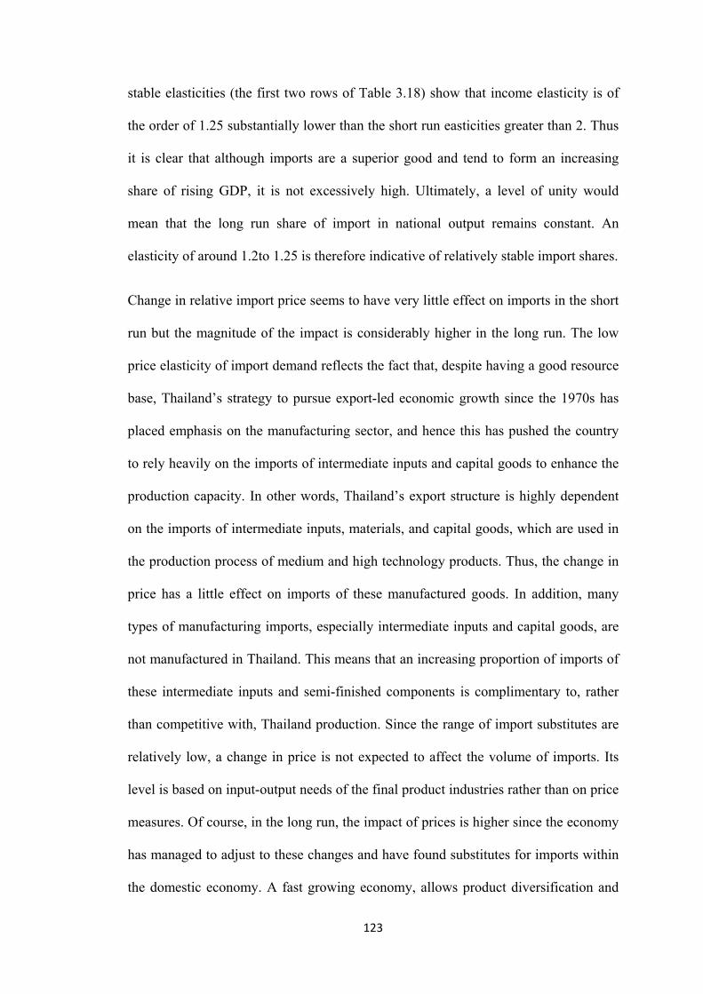
stable elasticities (the first two rows of Table 3.18) show that income elasticity is of
the order of 1.25 substantially lower than the short run easticities greater than 2. Thus
it is clear that although imports are a superior good and tend to form an increasing
share of rising GDP, it is not excessively high. Ultimately, a level of unity would
mean that the long run share of import in national output remains constant. An
elasticity of around 1.2to 1.25 is therefore indicative of relatively stable import shares.
Change in relative import price seems to have very little effect on imports in the short
run but the magnitude of the impact is considerably higher in the long run. The low
price elasticity of import demand reflects the fact that, despite having a good resource
base, Thailand’s strategy to pursue export-led economic growth since the 1970s has
placed emphasis on the manufacturing sector, and hence this has pushed the country
to rely heavily on the imports of intermediate inputs and capital goods to enhance the
production capacity. In other words, Thailand’s export structure is highly dependent
on the imports of intermediate inputs, materials, and capital goods, which are used in
the production process of medium and high technology products. Thus, the change in
price has a little effect on imports of these manufactured goods. In addition, many
types of manufacturing imports, especially intermediate inputs and capital goods, are
not manufactured in Thailand. This means that an increasing proportion of imports of
these intermediate inputs and semi-finished components is complimentary to, rather
than competitive with, Thailand production. Since the range of import substitutes are
relatively low, a change in price is not expected to affect the volume of imports. Its
level is based on input-output needs of the final product industries rather than on price
measures. Of course, in the long run, the impact of prices is higher since the economy
has managed to adjust to these changes and have found substitutes for imports within
the domestic economy. A fast growing economy, allows product diversification and
123

import demand can be reduced, with higher prices, because import substituting
industries have managed to develop.
run and long run, but the impact is quite small. As stated earlier, Thailand’s import
structure comprises the imports of interm
The reduction of Thailand’s average tariff rate seems to increase imports in both short
ediate inputs and capital goods in a high
For the export model, although the change in the world’s income appears not to have
ple, Houthakker and
proportion. In order to promote an export-led growth policy, the government
generally does not impose a tariff, or if there is one the rate is low, on these types of
products because the low input tariff makes it less costly to produce the final goods,
and thus improves the competitiveness of the country’s export goods. Instead, many
types of tariffs are imposed on final goods. Since raw materials, intermediate inputs,
and capital goods are imported at zero or low tariff rates, as a result, tariff reduction
does not have a substantial impact on Thailand’s import pattern.
a large immediate impact on exports, its impact is considerably high in the long run.
This evidence is consistent with other studies (see, for exam
Magee (1969)), that, in general, fast-growing countries seem to face a high income
elasticity of demand for exports. The empirical evidence of high income elasticity of
demand for exports has an important implication for exports of Thailand and other
developing countries in general. That is, the export growth of Thailand as well as that
of most developing countries is highly dependent on the economic performance of
developed countries. With reference to the high long-run income elasticity of demand
for exports, this can be implied that Thailand’s manufactured exports have a high
degree of exposure to its traditional export markets such as the U.S., Japan, and
among ASEAN countries. However, the effect of change in relative export price on
exports is very low in both short run and long run. On one hand, the low price
124

elasticity of export demand can be implied that the developing countries, including
Thailand, are not capable of using price competition to maintain or increase exports.
On the other hand, it can be implied that Thailand’s export markets are fairly
established. However, the high income elasticity of demand for exports could also be
viewed as an upward bias since there is an argument obtained from Krugman (1989),
that in the case of a high proportion of manufactured exports, the absence of a
variable to capture product quality improvements or product diversification will tend
to bias the estimated income elasticity of demand for exports upwards.
An interesting empirical observation from Table 3.18 is that the long run world
income elasticity of exports is similar to the long run domestic income elasticity of
imports (the former being somewhat higher). If for example, world income grew at a
economy as a result of the continued liberalization of trade and investment, the
similar rate as Thailand GDP, the impact on the trade balance would be negligible
since exports and imports would grow at a similar rate. In fact, because Thailand has
consistently grown faster than the rest of the world that there has been an enduring
issue about trade deficits.
Unlike the import model, world’s tariff reduction seems to improve exports of the
country in both short and longer terms. Through the increased integration of the world
manufacturing industries of Thailand have expanded significantly in terms of exports,
employment, and output. Manufactured exports have contributed significantly to the
growth and the economic development of the country. Currently, the bulk of
manufactured exports, which make up the largest share of the country’s total exports,
comprise the exports of computer and computer parts, transformer, generator and
motor, electrical appliances and electronic products, telecommunication equipments,
and integrated circuit. From the empirical result, Thailand seems to be successful in
125

gaining from the global tariff reduction since it is able to diversify its exports into
more manufactured goods and boost manufacturing through technology upgrading,
research and development, education and training, and these in turn strengthen the
country’s supply capacity.
To summarize, when comparing income effect between imports and exports, although
the magnitude of impact in long run is almost the same, the impact of change in
domestic GDP on imports seems to overwhelm that of a change in the world’s GDP
country. This can be inferred that global trade liberalization through the reduction of
he volume of imports
and exports in Thailand by means of the reduction of tariffs and joining AFTA and
itional import (export) demand functions
on exports in the short run. This may finally result in the problem in trade balance in
the short run, as stated above. However, this should not be a problem in the long run.
Thus policy makers need not be overly concerned about trade deficit unless it creates
a sort of currency and financial crisis of the past. Under ‘normal’ circumstances, the
trade negative balance will correct itself over time. The price effect on both imports
and exports is obviously very low in the short-run. However, in the long-run, it
appears that the impact of relative import price on imports is higher than the impact of
relative export price on exports.
Considering tariff reduction, the impact of world’s tariff reduction on exports seems
to be higher than the impact of Thailand’s tariff reduction on imports of its own
international tariff structures is beneficial for the country. It is clear that the various
WTO negotiations have overall benefited Thailand much more.
3.6. Conclusion
In this study, we analyze the impact of trade liberalization on t
the WTO membership by applying the trad
126

and then using the Autoregressive Distributed Lagged (ARDL) model to estimate the
short-run and long-run elasticities in Thailand’s import (export) demand over the
period 1960-2007. We also compared these estimates with the estimates obtained
using the cointegration techniques and an ECM. It turns out that the ARDL approach
and the cointegration and ECM approach give very similar results.
On one hand, in the aggregate import demand function for Thailand, the aggregate
import volume is cointegrated with Thailand’s GDP, Thailand’s relative import price,
and Thailand’s average tariff rate. On the other hand, in aggregate export demand
function for Thailand, the aggregate export volume is cointegrated with the world’s
GDP, Thailand’s relative export price, and the world’s average tariff rate. Results of
the estimated dynamic specification of the functions show that Thailand’s import
demand is largely explained by the country’s GDP, while Thailand’s export demand
is largely influenced by world’s GDP. As domestic income increases, Thailand’s
import expands more than proportionately. However, prices seem to have very little
effect on imports. This reflects the pattern of imports of the country that the country is
highly dependent on the imports of raw materials, intermediate goods, and capital
goods, such as mineral and metal products, chemicals and plastic materials, electronic
parts, and industrial machinery, industrial tools and parts, which are required in most
of the production process (also the production for exports), rather than consumer
goods and a substitution for domestic production. As for exports, it is found that
exports react moderately fast to a change in world income but relatively slowly to
movement in their relative price. The results of both import and export demand
functions are consistent with other studies, which generally find that developing and
industrial countries tend to have significantly higher income elasticities and lower
price elasticities.
127

In general, a country liberalizes its trade because it hopes that it will gain special
access to the market of its trading partner. More specific, a country agrees to reduce
or eliminate its trade barriers when it reaches agreement that other trading partners
at the expenses of other countries. In a world of tariff reductions, Thai imports will
will also reduce or eliminate their trade barriers. By this means, a country expects that
the loss from opening its market is overwhelmed by the gain from freer trade.
However, there is nothing to guarantee that every country participating in free trade
will experience a considerable increase in the volume of exports. Furthermore, if,
after trade is liberalized, exports do not increase proportionately as an increase in
imports, the trade balance will be worsened. High imports without a corresponding
increase in exports increase the trade deficit and further lead to current account
problem. Our results provide strong evidence that trade liberalization in terms of tariff
reduction promotes both imports and exports, with the impact of world’s tariff
reduction on exports is much higher than the impact of Thailand’s tariff reduction on
its imports. Thus, it can be concluded that, for Thailand, trade liberalization through
tariff reduction does not ultimately lead to the deterioration in trade balance per se. In
addition, liberalization in Thailand could be construed as a beggar-thy-neighbour
policy, in which Thailand can seek benefit from trade liberalization all over the world
rise but its exports will rise far more. However, we find no evidence of a statistically
significant effect of institutionalized trade liberalization, in terms of joining AFTA
and the WTO, on both imports and exports.
128

Chapter 4
ESTIMATING THE IMPACT OF
TRADE LIBERALIZATION ON TAX REVENUE
129

4.1. Introduction
While trade liberalization has long been investigated by a number of studies and
believed to provide benefits for those countries which promote freer trade by inducing
trade creation, lowering consumer prices, raising countries’ welfare and increasing
h
competition for the domestic economy which finally may help domestic markets
reach higher efficiency16, very few studies paid attention to issues concerning the
consequence of trade liberalization decreasing tax revenues, not only on international
trade taxes as a result of tariff reduction, but also on domestic taxes as a result of
erosion of tax bases. T is leads to a controversy whether trade liberalization is a
potential source of fiscal instability, especially for countries which have high
dependency on trade tax for their public revenue. Each step in liberalizing trade for
many developing and less developed countries is now very sensitive because it raises
the issue of revenue losses which may continue to be a very big problem for any
budget-constrained government where trade tax is the major revenue source of the
country. Although it is found that trade taxes are not a significant source of revenue in
OECD countries since they are accounted for only 0.5 percent of total tax revenues,
the dependency on trade taxes is much higher in middle income countries; around 16
percent in average. The fear of the impact of trade liberalization seems to be
substantial in low income countries because the percentage of trade tax in total tax
revenues is as high as 26 percent on average.17 Because of such a high dependence on
trade tax for revenue, any country which has that tax structure and commits itself to
any form of trade liberalization must be concerned about how to mitigate the revenue
loss, a serious problem that trade liberalization potentially entails.
16 See Viner (1950), Lipsey (1957), Kemp and Wan (1976), Wonnacott and Lutz (1989), Krugman (1991) and Summers (1991) for example. 17 See Pelzman (2004).
130

There are some studies suggesting that the revenue problem can be solved if trade
liberalization is co-ordinated with potential government budget spending, sound
macroeconomic policies, and effective measures on tax revenue, including raising
18
complicated than that of trade tax, so the replacement from these alternative sources
through the liberalization process, the trade tax continues to be a major source of
domestic direct and indirect taxes, widening and developing new tax bases, improving
effectiveness of public spending, raising public saving, and strengthening tax
collection and administration. However, what is good in theory may not be
applicable in practice. Many countries find it is very difficult to implement these
responses in order to prevent the adverse effects on fiscal revenues. The reason that
most developing and less developed countries usually rely heavily on trade tax is not
only because of the ease of collection, but also because they have some constraints.
Their restrictions may have various explanations such as the political instability, the
constrained institutional capacities, and the limitation of a country’s geography.
Generally, countries, which have a small geographical area, tend to have small
domestic market, small population size, and un-diversified production. These
attributes result in narrow tax bases, leading to the difficulty in switching revenue
sources from trade tax to other domestic taxes. In addition, the structure of income
and consumption taxes, especially for Value Added Taxes (VAT) is much more
requires a good design of country’s tax practice reform. Developing and less
developed countries always face the problem of domestic tax reform because of their
relative lack of skillful authorities and efficient tax system. Moreover, the empirical
work constructed by Pelzman (2004) suggests that, although countries may be going
revenue, especially for budget-constrained countries. Increases in domestic taxes, in
18 See Peters (2002), Mujumdar (2004), Keen and Ligthart (2004), and Glenday (2000) for example.
131

order for countries to compensate for the loss in tariff revenue, yield diminishing
returns. He also finds that as domestic taxes increase, more and more economic
activities are pushed into the informal sector. Hence, he concludes that trade
liberalization tends to have a negative impact on the domestic revenue for developing
countries. The level of countries’ economic development also has a significant
influence since developing and less developed countries generally have relatively low
institutional quality, corrupt governments, and low technology, causing a problem in
the improvement of tax collection and administration. Cutting down the government
expenditure as a consequence of the decrease in revenue seems not to be feasible
since it directly reduces welfare. In addition, government spending on the social
sector, infrastructure, national defense, and poverty reduction cannot easily be cut
because it may also raise political issues. If it chooses to do this, the government may
easily be pressured by affected groups and those who oppose free trade.
Although some countries are able to cope with the negative fiscal effects of trade
liberalization by using a mix of tax and non-tax policy, the non-tax policy seems to
play a limited role. The results of non-tax policies such as improving macroeconomic
performance, controlling inflation, controlling public spending, and increasing the
reliance on non-tax revenues are likely to be uncertain and these policies are able to
be accomplished only in the long term. The most possible efficient alternative to deal
with fiscal difficulties in the short and medium term is to use the tax policy response
by introducing domestic tax reforms, for both income and consumption taxes.
However, since trade liberalization could possibly lead to a reduction in output,
corporate profits, and employment in certain sectors that face greater competition
from lower-cost foreign products, this impact on domestic tax bases could finally
result in the reduction of domestic taxes. Although the net outcome depends crucially
132

on many factors such as the flexibility of wages and prices to allow the full
adjustment of relative prices after trade is liberalized, the ability of domestic firms to
face higher competition, the structure of economy, and the structure of country’s tax
system, the adverse effect of trade liberalization on domestic tax revenues is an
important issue to be taken care of when a country walks along the liberalization path.
For many developing and less developed countries, the loss of trade tax revenue is
itself a very big problem. If trade liberalization is also associated with the reduction in
other domestic tax revenues, it will be a much hard work for governments in these
countries to pursue domestic tax reform by substituting their sources of revenue from
trade taxes to income and consumption taxes which may consequently end up with
unsuccessful replacement, and hence the failure of tax reform.
Although a large number of studies have tried to investigate the net impact of trade
liberalization on trade tax revenue, very little attention has been devoted to examining
the impact of trade liberalization on domestic taxes. The aim of this chapter is to
examine the effect on both trade taxes and domestic taxes after trade is liberalized,
focusing particularly on low and middle income countries. This chapter attempts to
investigate this issue by adopting the traditional tax effort model, using a panel data
approach for 134 countries over 24 years covering the period 1980-2003 and
employing the two-way fixed effects approach.
This chapter is organized as follows: the next section is devoted to a brief literature
review. Section 3 provides a background for the traditional tax effort model. Section 4
describes the extended model, data, and estimating procedure. Section 5 presents and
discusses the results for full sample and each income group. Section 6 concludes the
chapter.
133
4.2. General Review: Theoretical and Empirical Background on the Relationship
Between Trade Liberalization, International Trade Tax, and Domestic Taxes
ile
ces
s to lower trade tax revenue.
developing and less developed countries which decide to liberalize trade. Aizenman
trade openness and financial integration by taking them as exogenous factors. From
In this section, the literature survey starts with some notable works pointing that it is
possible for countries to be unsuccessful in implementing domestic tax reform wh
they are in the process of trade liberalization. Some restrictions are revealed since
they possibly account for the failure of tax reform. Then, some related studies are
reviewed to highlight how trade liberalization may affect each type of taxes.
4.2.1. The Failure of Revenue Source Substitution
The most obvious way of how trade liberalization affects tax revenue is that it redu
trade restrictions including tariffs, and hence tend
However, the relationship between trade liberalization and other domestic tax
revenues is still ambiguous, or even the impact on trade tax revenue itself is an
empirical matter. Compared with the studies of free trade related growth,
employment, or trade creation and diversion, there have been a relatively small
number of both theoretical and empirical studies on the revenue impact of trade
liberalization. Among the studies, there is an attempt to investigate the possibility of
mitigating the decrease in trade tax revenue since this is the major concern of most
and Jinjarak (2006) study the relationship between globalization and the changes in
the “easy to collect” and “hard to collect” taxes; defining the “easy to collect” taxes
are the revenues from tariff and seigniorage, while the “hard to collect” taxes are the
revenues from Value Added Tax (VAT), and using two measures of globalization;
the hypothesis that globalization may lead to a reduction of the countries’ tax
134

revenues, especially for most developing countries, by shifting tax base from “easy to
collect” to “hard to collect” taxes, they show that the revenue of “easy to collect”
taxes declined by about 20%, while the revenue of “hard to collect” taxes increased
only 9% between the period 1980-1999.
The results of Aizenman and Jinjarak (2006) seem to be supported by the work of
Baunsgaard and Keen (2005). They examine whether countries can recover their loss
taxes and they may not be able to recover their loss of trade tax
of trade tax revenue, as a result of trade liberalization, from increasing domestic tax
revenues by running regressions on both full sample and three separate groups; low,
middle, and high income countries. The results show that, for the full sample,
although openness is significantly positively related to domestic tax revenues, its
impact is quite small. The degree of revenue recovery is only 20 to 50 cents per
dollar. For low income countries, openness is positively significant with a stronger
impact than that of full sample. However, the recovery rate is the lowest; less than 30
cents per dollar. For middle income countries, openness is still positively significant.
The recovery rate is a bit higher, from 45 to 65 cents per dollar. For high income
countries, openness is insignificant in all specifications. However, the recovery rate is
more than offset since domestic tax increases from 1.5 to 3 dollar, especially for those
which adopt VAT.
In addition to the evidence that countries may fail to shift their tax bases from trade
tax to other domestic
by raising domestic tax revenues, there is also evidence that trade liberalization itself
is likely to hinder the substitution of tax revenues. Agbeyegbe, Stotsky, and
WoldeMariam (2004) construct an empirical study using panel data of 22 countries in
Sub-Saharan Africa over 1980-1996 to address the question whether trade
liberalization leads to a reduction in total tax revenues through its effect on
135

international trade tax and other domestic taxes. The results strongly support the
uncertain effect of trade liberalization. Although the results suggest that trade
liberalization leads to stronger total tax revenues and trade tax revenue, there is
evidence that trade liberalization is associated with weaker income tax and goods and
services tax. A reduction in domestic taxes may potentially result in the difficulty of
replacing sources of revenue.
Even if trade liberalization has no effect on domestic taxes, tax reform is a very
difficult task for many less developed and developing countries to pursue. Now, if
ese countries tend to be highly dependent
trade liberalization has a negative impact on domestic tax revenues, reform by using
these sources may be inapplicable. This raises the question whether these countries
should implement the reform in the same way as developed countries. What is the
difference between these countries and most developed countries? In the next section,
the exploration of some unique features of developing and less developed countries is
provided in order to investigate their restriction which may cause the failure of tax
reform.
4.2.2. Characteristics of Developing and Less Developed Countries: Self
Constraints
The impact of trade liberalization seems to be substantial in developing and less
developed countries since the revenue of th
on international trade tax. Actually, these countries have long used trade tax and
subsidies, import and export quotas, and other non-tariff barriers to adjust their
international trade. The traditional trade tax has been used to achieve two major
purposes; increasing revenue for the public sector and protecting their infant and local
industries. However, since the beginning of the liberalization period, many industrial
136

nations have attempted to promote the high and sustainable growth to the global
economy. One of their policies is to pursue global trade liberalization through the
World Trade Organization (WTO) or Free Trade Agreements (FTAs). No matter how
well the economic structures of developing and less developed countries are prepared
or no matter how willing they are to liberalize their trade, they have already and
automatically been forced to walk along the path of globalization and liberalizing
programme.
As stated in Khattry and Rao (2002), policy options which are developed for
advanced economies are not appropriate and cannot be implemented in low and
1. Geographical constraints
The size disadvantages have widely and obviously been observed in standard
mall country has a small domestic market which results in
middle income countries since they possess unique features which are the important
constraints and cause the transition problematic. Those limited features can be
categorized into three groups.
economic theories. First, a s
industries being unable to obtain economies of scale. Second, a small nation tends to
have less domestic competition within its internal market which leads to an inefficient
allocation. Third, as it is pointed by Helpman and Krugman (1985) about the lack of
strategic trade policy, a small nation has less potential in preparing their domestic
firms to enter the world market and it also has limited potential to use import-
substitution policy. Fourth, many small nations have poor domestic resources, leading
to a narrow range of domestic output. As a result, these countries are highly
dependent on imports and exports which make them quite vulnerable to external
economic shocks.
137

Smallness does not only have an impact on production, allocation, and competition as
stated above, size also affects a country’s tax receipt. Since small and less developed
nsumption tax such as VAT. For instance, while a trade tax imposes
predominant arguments is that the tax base of a consumption tax is generally much
countries tend to have high dependence on trade tax for their revenue, trade
liberalization, especially by the reduction of tariffs, severely seems to decrease trade
tax revenue, and hence causes fiscal problems. According to Peters (2002), he
explores the fiscal effects of trade liberalization for the Caribbean Community
(CARICOM), as the case of small open economies, by using descriptive analysis and
concludes that because CARICOM possesses two restrictive characteristics; small
size and low level of development, these countries usually have small domestic
markets and un-diversified or even mono-production. These features force this
community to be highly dependent on external trade and have narrow tax bases. He
also points that although the magnitude of the impact of trade liberalization is difficult
to assess, there could be a shortfall in the short-run trade tax revenue as much as 45
percent. The mitigation of the decline in revenue by introducing broad based
consumption taxes (i.e. VAT) seems to be difficult due to the many countries’
restrictions such as the size of domestic markets and the level of economic
development.
There are several traditional arguments for substituting trade-based tax to more a
broad-based co
distortions on both consumption side and production side, consumption taxes distort
only consumption, hence a trade tax generates more distortion and a consumption tax
is more preferable than a trade tax. Among those reasons, one of the most
larger than that of a trade tax so a consumption tax could potentially be used to
mitigate the loss of trade tax receipts or even to raise overall tax revenues. However,
138
this argument is likely to be practicable only for large size countries because in order
to gain the revenue from the consumption tax, a large consumption base is needed. It
is very difficult for small countries to raise a considerable amount of consumption tax
revenue since they have only a small domestic market and hence limited
consumption. In addition, there is some evidence that poverty levels and income
distribution tend to be more uneven in smaller than in larger countries. This may also
push the level of consumption in small countries down and as a result reduce the
amount of consumption tax collection.
However, the problem of fiscal compensation for lost revenue from trade
liberalization is not likely to be limited in small countries. Rajaraman (2003) attempts
to investigate where the fiscal compensation can be sourced by using descriptive
analysis and reviewing the literature since he finds that the loss in tariff revenues in
India have resulted in diminishing aggregate tax revenue. Although the theoretical
results from Keen and Ligthart (1999) suggest that the loss in tariff revenues can be
replaced by domestic indirect taxes, more specifically a price-neutral VAT and
conclude that VAT could enhance both revenue and welfare, the empirical work using
cross-country regressions for 183 countries of Ebrill et al (2001) shows the
contradictory results that VAT is not significant in raising tax revenues.19 Together
with the lack of empirical evidence on revenue enhancement by VAT adoption,
Rajaraman (2003) concludes that there is not enough evidence to ensure that India’s
loss in trade tax revenue can be compensated by a consumption tax.
19 Note that openness is also included in the regression as one of tax revenues determinant and it is found that openness has a significant positive impact on tax revenues.
139

2. Structural constraints
“Economic Development with Unlimited Supplies of Labour”, Lewis (1954)
odel and demonstrates that a country becomes more
urbanized as its economy grows. As countries develop, it has been observed that tax
because they compose
dispersed, small-scale firms and produce primary products which are associated with
In
constructs a two-sector m
bases grow more than proportionately to the growth of income. That is the capacity to
tax grows with the growth of GDP (Musgrave, 1969). Supported by later work, Tanzi
(1987) studies the relationship between tax levels and economic development and
conclude in the same way that, as countries grow, they become urbanized.
Urbanization leads to an increase in both the need for tax revenue and the capacity to
tax. On the demand side, urbanization leads to higher demand for public services and
hence the government needs to raise more income from tax revenue in order to
support its public activities. On the supply side, urbanization leads to larger tax bases
and higher development in public services facilitating tax collection which in turn
improves the capacity to tax of the government.
Unlike developed economies, low and middle income countries tend to be more rural.
Rural economic activities are much more difficult to tax
the subsistent economy rather than commercial economy. Even if there is a surplus for
commerce, these firms often escape tax collection. In addition, because these firms
are informal in their nature, their income is very difficult to assess and hence it is hard
to include them in the income tax base. As a result, the government usually levies
taxes on agricultural exports which is much easier instead of attempts to assess their
income. This is one of the reasons why low and middle income countries tend to have
a high proportion of trade tax in their total tax revenues. Moreover, most population in
less developed and developing countries tend to be children and elders, falling in the
140

age-dependency group. With a high age-dependency ratio, the income tax bases in
less developed and developing countries are much narrower than income tax bases in
developed countries. These aspects limit the possibility to substitute sources of tax
revenues from trade tax to income tax when tax reform is preceded after trade
liberalization.
3. Institutional and political constraints
Institutional quality has a direct effect on a country’s tax collection. In less developed
and developing countries, there is weak management, with poor information, auditing
ith inefficient and high corruption tax and supervision of staff, in line w
administrations, leading to the difficulty in assessing taxes. These factors, when
combined with high tax evasion as a result of the weakness of the rule of law and the
lack of administrative capacity, result in low level of tax revenues in low and middle
income countries. These features contribute to the use of trade tax in these countries
because, when compared with income base tax or consumption base tax, trade tax is
relatively easy to assess and monitor and has less problems of tax evasion.
In low and middle income countries, there is also political obstruction which impedes
the domestic tax reform and domestic tax base expansion. The influence of powerful
lobbies makes some sectors be exempted from taxation. It is demonstrated by
Ndikumana (2001) that political power used by some interest groups results in
lobbying and tax exemption. This results in the limited use of both personal income
and corporate income taxes. In addition, it is found that low quality institution and
political instability have a negative influence on goods and services tax collection
(Aizenman and Jinjarak, 2006). Thus, it can be concluded that low quality of
institutional factors is an obstruction to the mitigation of the loss in trade tax.
141

So far, we have investigated the reasons why a country may fail to recover the loss in
trade tax revenue and be unsuccessful in reforming its domestic taxes by using the
explanation of country’s attributes and excluding the effect of trade liberalization on
Trade liberalization may have a different impact on different kinds of tax revenue.
e revenue impact of trade liberalization
nal trade tax, personal
in import tariffs,
ralization, often leads to a drop in trade tax revenue,
case of countries in the Caribbean community which are constrained by having a
leads to a reduction in trade tax receipt and finally a decrease in total tax revenues.
tax revenues from the frame. In the next section, we introduce trade liberalization into
the picture and review the studies which show how trade liberalization may affect
each tax type.
4.2.3. The Effect of Trade Liberalization on Tax Revenues
This section reviews the literature studying th
by dividing tax revenues into 4 categories, including internatio
income tax, corporate income tax, and goods and services tax.
1. International Trade Tax
Generally, international trade tax revenue is thought to decrease after countries
liberalize their trade. Many studies point out that the reduction
associated with trade libe
especially for small open economies which their tax revenues tend to be more heavily
dependent on international trade. Peters (2002) investigates this issue by taking the
small size and lower level of development. Although the trade tax revenue effect of
trade liberalization is generally uncertain depending on many factors such as
countries’ conditions, initial position of tariffs, and the level of import elasticities of
substitution, he finds the evidence that trade liberalization in these countries usually
142

Ebrill et al. (1999) provide a clear-cut explanation of the effect of trade liberalization
on trade tax. They state that the revenue implications depend largely on the volume of
imports after trade is liberalized. Generally, trade restrictions are composed of two
restrictions (Figure 4.1). When the initial tariff rate is prohibitively high, trade
reduction after trade is fairly liberalized at the revenue maximizing rate, the increase
major components, tariff barriers and non-tariff barriers. Although the main aim of
trade liberalization is to reduce or eliminate both restrictions, most liberalization
usually considers the removal of quantitative restrictions at the first phase and then
the continual reduction of tariff rates in the second stage. They reason that goods,
which are restricted by quotas, usually are tariff imposed. If quotas of these goods are
removed, it is possible that trade tax revenue may increase at least in the very first
stage of liberalization as the volume of imports is likely to increase. This may also be
true in the case of the replacement of quantitative restriction such as quotas by tariffs.
The initial tariff levels, their coverage, and the extent to which they are reduced, play
a significant role in determining the impact on international trade tax revenue. Ebrill
et al (1999) reason that if the initial tariff rates are high, tariff reduction may lead to
an increase in trade tax revenue since price elasticities of demand and supply are not
constant over the entire range of prices. This effect can be illustrated by a Laffer
curve, which demonstrates the relationship between trade tax revenue and trade
volumes are likely to be severely compressed and trade tax revenue will be very low.
Reducing tariffs will lead to a substantial increase in trade volumes and a decrease in
the incentive to evade taxes. These combinations are more than compensating for the
lower tariff rate, which results in higher tariff revenue. However, if there is a further
in trade volume will not be large enough to offset the lower tariffs and now the direct
effect of tariff reduction will result in the loss of revenue. As a result, overall tariff
143

revenue will therefore decrease (Ebrill et al, 1999; Khattry and Rao, 2002; and
Agbeyegbe et al, 2004).
Figure 4.1: Laffer Curve
Ebrill et al (1999) also mention that if the liberalization is accompanied with the
reduction in tariff dispersion, trade tax revenue may increase. The rationale is that a
reduction in the dispersion of tariffs is often done by lowering the higher tariffs and
increasing the lower ones in order to reduce them to average value and usually, highly
elastic demanded goods such as final consumption goods stated above are also high
tax levied. As a result, a reduction in tariff dispersion may lead to an increase in trade
tax revenue. In addition, the reduction in tariffs is often associated with the reduction
of tax evasion and tariff exemptions. It is intuition that the higher the tariffs, the
higher the tax evasion since evasion leads to high marginal benefit for importers.
Many works find that there is a positive relationship between tariff rates and tax
Tariff Rate
Trad
e Tax Re
venu
e
Revenue Maximizing Rate
144

evasion.20 Recent research shows empirical evidence that a one percent increase in
tariff rates is associated with a three percent increase in tax evasion (Fisman and Wei,
2001). The tariff reduction, of course, raises the costs for tax evaders and hence
lowers the level of tax evasion, thus it may bring an increase in trade tax revenue. For
tariff exemptions, Pritchett and Sethi (1993) find that high tariff rates do not necessary
lead to high trade tax revenue. Very similar to the case of tax evasion, they argue that
higher tariff rates lead to higher incentives for importers to attempt to seek
exemptions. The reverse relationship is also true. The lower tariff rates may not bring
a decrease in trade tax revenue since the temptations for abuse of any system of
exemptions will decrease with the lower level of tariffs.
Trade tax revenue may also depend on the price elasticity of demand for imports and
the price elasticity of supply of import substitutes. According to Ebrill et al (1999)
and Agbeyegbe et al (2004), if either the price elasticity of demand for imports or the
price elasticity of supply of import substitutes is high enough, there may be revenue
gain in later stage of liberalization if the new value of imports (higher volume of
imports multiplied by lower tariff rates) exceeds the value of imports before
liberalization take places. The volume of imports can be increased in two ways. On
one hand, since the prices of imported goods are cheaper after the restrictions are
removed, if the price elasticity of demand for imports is elastic enough, the volume of
imports may increase to the point which import values offset the loss from tariff
reduction. On the other hand, the prices of import substitutes domestically producing
are forced to be lowered when imported goods increase due to competition. As a
result, domestic output decreases and thus imports increase. However, the elasticity
issue might be very complicated because it depends on the timing and characteristic
20 See Clotfelter (1983), Fisman and Wei (2001) for example.
145

of each good. Generally, imported consumer durable goods respond to the price
changes more than do intermediate goods and raw materials (Clarida, 1996). In
addition, most countries always reduce their restrictions from raw materials,
intermediate goods to final consumption goods which are usually import competing
goods, consecutively, in order to avoid political contention (Ebrill et al, 1999). In this
case, an increase in trade tax revenue may occur only in later stage when tariffs of
final consumption goods, which are often taxed at high rates, are eliminated.
Trade liberalization does not only involve the reduction or removal of tariffs and
quantitative restriction, but it may also involve the reduction or elimination of an
export tax. Similar to the case of tariff cut, if the reduction of the export tax leads to a
substantial increase in a country’s export volume, a country may be able to collect
more trade taxes. However, if the reduction of an export tax does not bring about a
significant increase in export volume, trade tax revenue will be decreased.
However, countries may have a revenue problem due to the deterioration of their
terms of trade.21 It is possible that when many developing and less developed
countries liberalize their trade simultaneously, there will be an excess supply of
similar products which could lower the export prices and finally could exacerbate
their terms of trade. This could directly affect a country’s export sector and severely
worsen export tax revenue.
In conclusion, it is very difficult to determine precisely the effect of trade
liberalization on international trade tax revenue since trade liberalization may either
decrease or even increase trade tax revenue, depending on the form, the level of
liberalization and countries’ environmental liberalization conditions. The net impact
21 See Devereux and Chen (1999) for example.
146

of trade liberalization on trade tax is an empirical matter. Trade tax revenue may also
be affected by other important variables such as the level of economic development,
the exchange rate, the macroeconomic environment, and the effectiveness of tax and
customs administrations (Ebrill et al, 1999).22
2. Personal Income Tax
There seems to be no direct effect of trade liberalization on personal income tax.
Trade liberalization, however, is likely to transmit its contribution to personal income
tax revenue through economic growth. Ebrill et al (1999) point out that there is now
considerable empirical evidence that trade liberalization is related to the higher level
of economic growth. Frankel and Romer (1999) construct an empirical study to
investigate the effect of trade on income by applying the gravity model and using
geographic factors as an alternative instrument for trade. They find that trade
substantially raises income since a one percent increase in the shares of imports and
exports in GDP leads to a one-half to two percent increase in income per person. This
means that trade liberalization which induces higher volume of trade is associate with
higher income growth. Frankel and Rose (2000) estimate the consequences of
currency unions that have on the long-run level and rate of growth of real income, via
trade. The most interesting part of their study is the substantial impact of free trade
agreements, a form of trade liberalization, on international trade in which they find
that free trade agreements roughly triple the trade between countries. They suggest
that the contribution of currency unions to an economy comes from the higher volume
of trade which occurs as a result of trade encouragement after countries join the
22 The effect of exchange rate on tax revenue is still ambiguous as the results from different studies are mixed. For example, using the same data set and similar approach, Adam et al (2001) find a significant relationship between exchange rate and tax revenue, while Agbeyegbe et al (2004) find no evidence supporting the relationship between them.
147

union, rather than macroeconomic or financial influences. The benefit to a country’s
economy from being a member of a currency union comes through the promotion of
trade, rather than through the benefit from any monetary policy as proponents of
currency unions advertise. A more recent study, Baier and Bergstrand (2005)
construct a gravity framework using differenced panel data and find that the effect of
free trade agreements on trade flows is almost quintupled, again supporting the
hypothesis that free trade agreements lead to an increase in trade volume which
stimulates economic growth.
Economic growth is likely to have a direct impact on both personal income tax and
uch less
total tax revenues. Higher per capita income leads to a wider personal income tax
base. Many previous literatures reached a conclusion that there is a significant
positive relationship between economic development and personal income tax
revenue. For instance, Musgrave (1984) provides a solid theory supporting a causal
relationship between per capita income and tax level in his tax base and tax handle
theory. He states that an increase in per capita income raises the size of public sector
which in turn increases a country’s tax base and taxable capacity. Tanzi (1987)
demonstrates the association between economic growth and tax by using regression
analysis and found in the same way that overall tax revenue is positively influenced
by the level of per capita income. Although the correlation is not strong, he also finds
that per capita income growth has a positive impact on personal income tax.
However, it is pointed out by Tanzi (1987) that personal income tax is m
important in developing and less developed countries than it is in developed countries
(in terms of actual collection). This may be due to the difficulty in assessing personal
income, high administrative costs and other structural constraints. As stated in
Aizenman and Jinjarak (2006), most developing and less developed countries have
148

low level of investment in their tax capacity, leading to poor ability of auditing. In
addition, personal income tax, in those countries, is relatively easy to be evaded
because most developing and less developed countries generally have weak penalty
on tax evasion and structural factors that increase the ease of tax evasion. Moreover,
in developing and less developed countries, personal income tax is usually levied on
wages of public sector employees and the employees of the large, and often foreign,
corporations (Tanzi, 1987). All of these depress the personal income tax base,
resulting in a narrower base in developing and less developed countries than in
developed countries, and hence lower revenue from this tax.
Inflation is another factor which may affect personal income tax. There is large a
literature on the effect of inflation on taxation, especially in the 1970s and early 1980s
when inflation was high. Most studies suggest that the impact of inflation on personal
income tax could be considerably large. Inflation may affect personal income tax,
especially for capital gain tax, by leading to an increase in effective tax rates because
this tax is computed as a fraction of changes in nominal value.23 Theoretically,
inflation affects income tax in three ways; altering real factor incomes, affecting the
measurement of taxable income, and changing the real value of deductions,
exemptions, credits, ceilings and floors, bracket widths, and all other tax provisions
legally fixed in nominal terms (Aaron, 1976). There are also many empirical studies
which prove their relationship, for example, Greytak and McHugh (1978) point that
there is a substantial increase in personal income tax revenue, occurring as a result of
purely a nominal increase in income which appears during inflationary periods. The
large increase of tax receipts is due to the progressive nature of this type of tax.
23 See Aaron (1976), Bailey (1976), and Tanzi (1980) for example.
149

3. Corporate Income Tax
und to be more important to less developed and developing
rade liberalization on corporate income tax is also very difficult to
income tax.
Corporate income tax is fo
countries. In these countries, corporate income tax is usually collected from a few
large corporations which have sizable profits. In addition, taxing a few large firms is
administratively easy for government in less developed and developing countries
(Tanzi, 1987).
The effect of t
estimate. Like international trade taxes, how trade liberalization affects corporate
income tax depends on many factors such as the volume of trade, the price elasticity
of demand for imports and the price elasticity of supply of import substitutes, and the
initial domestic prices. If trade liberalization leads to a higher volume of imports or
exports, import and export companies, which generally have a large share of output in
most less developed and developing countries, may benefit from increasing volume of
trade and consequently result in higher corporate income tax. After trade is
liberalized, there is the price adjustment of import goods and domestic goods. If the
initial prices of domestic goods are lower than the prices of import goods, the
domestic production of import substitutes is likely to be increased because domestic
prices are higher after a country liberalized its trade. Consequently, a tax on corporate
income which is derived from the increase in production of import substitutes should
increase. However, if the relative prices of import substitutes are higher before trade
is liberalized, trade liberalization tends to lower domestic prices and decrease the
production of domestic goods, and hence lower corporate profits and corporate
150

The deterioration in terms of trade, which possibly occurs when countries that export
the same or similar items liberalize simultaneously, could potentially affect corporate
income tax revenue. Because exporters now export less, income earned from exports
decreases, and hence corporate income tax collected from export companies tend to
be diminished.
Like personal income tax, trade liberalization influences corporate income tax through
the growth effect. Generally, firm’s profits grow with the growth of the economy.
Tanzi (1987) finds a significant positive relationship between economic growth and
corporate income tax. He also points out that the impact of economic development on
corporate income tax is greater than on personal income tax.
4. Goods and Services Tax
Tax on consumption is usually considered as a good solution for offsetting the
decrease in fiscal revenue since a consumption tax has broader base and distorts the
economy less than a trade tax (e.g., Keen and Ligthart, 1999; Peters, 2002; Mujumdar,
2004; Baunsgaard and Keen, 2005).24 However, the impact of trade liberalization and
other physical constraints may make the domestic tax reform a lot harder for
developing and less developed countries. The impact of trade liberalization on goods
and services tax is more complicated to assess since the effect is indirect and also
depends on many factors such as the price elasticity of demand for imports and the
price elasticity of supply of import substitutes. For example, when tariffs are reduced,
the relative price of imports to import substitutes produced domestically decreases,
24 Although the substitution from trade tax to consumption tax is acceptable, an increase in domestic consumption tax as a strategy of offsetting reductions in tariffs is later refused by Keen and Ligthart (2004). They reproduce model under imperfect competition and find that an increase in consumption tax rate potentially reduces overall domestic welfare, contrary to the model formed under perfect competition in Keen and Ligthart (1999) in which they find umambiguous benefit.
151

and hence domestic consumers tend to switch their consumption from domestically
produced import substitutes to imports. This leads to a decrease in tax revenue
collected from domestically produced import substitutes and an increase in tax
revenue obtained from imports. However, the net change in tax revenues cannot be
generally predicted.
The domestic tax reform itself by switching the reliance of taxes from international
trade tax to consumption tax may also affect the revenue. If the domestic consumption
tax is levied only on domestically produced goods (import substitutes), trade
liberalization tends to lowers the revenue from domestic indirect tax. But, if taxes are
levied on both imports and domestically produced goods, goods and services tax tends
to be increased. Ebrill et al (1999) state that trade liberalization may affect goods and
services tax revenue if the imported goods, which their tariffs are reduced, are
included, at a significant proportion, in the domestic tax base. The direction of its
impact depends on the volumes of imports after trade is liberalized. If there is no
significant change in import volumes, leading to an unchanged import values, trade
liberalization may immediately lower goods and services tax revenue. However, if the
import volumes increase at a significant level, goods and services tax revenue may
also increase.
The indirect effect of trade liberalization on goods and services tax revenue can also
be viewed through its impact on economic growth, like personal income and
corporate income taxes as stated above. Because tax bases grow as countries grow,
this should also be true for the consumption tax base since its base also relates to the
growth of income. People should have more money in their hand as GDP grows,
which means that there is higher purchasing power and higher demand for domestic
consumption. However, surprisingly, the results shown in Tanzi (1987) stated that
152

there is no correlation between the share of domestic tax on goods and services in
GDP and per capita income.
Besides economic growth, a country’s size could play an important role in
determining the domestic consumption tax (Peters, 2002). Generally, a consumption
tax is a more significant revenue source in the bigger countries than in the smaller
countries because the amount of tax collection depends directly on the domestic
consumption. Larger countries tend to have a high population and a large domestic
market whereas smaller countries seem to have less population and their size of
domestic market is smaller. As a result, switching sources of revenue from a trade tax
to a broad-based consumption tax, although applicable for developed countries, may
cause fiscal problems for developing and less developed countries.
In conclusion, the empirical literature on trade liberalization and taxation supports the
claim that the net effect of trade liberalization is uncertain and the net change in tax
revenue as a result of liberalizing trade is an empirical matter. In addition, the impact
on each tax type depends on many different factors. The following section applies the
traditional tax effort model and employs an econometrics approach in order to
investigate further the relationship between trade liberalization and countries’ tax
revenue.
4.3. The Basic Model of Tax Effort
A considerable number of studies have attempted to find measures of fiscal
performance. In previous works, the tax ratio has always served as a rough index of a
country’s tax performance or a measure of the relative effort of a country.25
Generally, tax ratio analysis aims to explain the main determinants of differences in
25 See Bahl (1971), Ansari (1982), and Stotsky and WoldeMariam (1997) for example.
153

the tax ratio across countries. Most research concludes that the reason why there are
such differences is because countries have different “capacities” to tax. Among early
studies, Musgrave (1969) makes a great contribution to the explanation of why less
developed countries usually have a low level of tax revenue by presenting a key term,
“Tax handles”. Tax capacity or tax handle has been introduced as a key to increasing
tax effort. For low income countries, it is much more difficult to impose and collect
taxes than in an advanced economy. He reasons that it is not only the skills and
facilities of tax administration in those countries that are less developed, but also the
structure of their economies can afford fewer and less adequate “handles” on which to
collect taxes. Thus, the relative absence of adequate tax handles in less developed
economies is a main reason in explaining why their tax to GDP ratios is lower than
those of highly developed economies.
In the previous studies, a variety of methods have been tried to estimate tax effort.
However, the most commonly used approach is to regress the tax performance on
variables that serve as proxies for a country’s tax handles. This means that the
independent variables used in this approach are represented as the major determinants
for tax effort. By regressing tax effort, the stochastic model is used where T is the
total tax revenue, Y is a proxy for income (either GDP or GNP), and T/Y is the tax
ratio. The independent variables which are expected to influence the tax ratio are
represented by Xi (i=1, 2,…, n) and u is the error term. This can be expressed in the
following functional relationship:
/ ( ,..., , )i nT Y f X X u= (4.1)
The most traditional explanatory variables in the conventional tax effort studies are
those controlling for a country’s economic structure. These variables reflect the idea
154
that the availability of tax handles influences the level of tax effort. The following is
the list of explanatory variables suggested by economic theory and by many previous
empirical works. An overview of empirical results from some related literature is
summarized in Appendix 4A. The independent variables that have been widely used
by previous research are:
(1) Level of Economic Development: measured by GDP per capita. Higher income,
reflecting a higher level of development, is usually associated with higher
capacity of tax payers to pay taxes as well as a greater capacity of the
government to collect taxes from them. In addition, rich countries tend to have a
higher degree of monetization of the economy and better tax administration
(Agbeyegbe et al., 2004). Moreover, rich countries often tax proportionately
higher than poor countries. Hence, it is expected that there is a positive
relationship between the ratio of total tax revenue to GDP and GDP per capita.
(2) Composition of GDP: measured by the share of the agricultural sector and the
industrial (including mining) sector in GDP. The share of the agricultural sector
in GDP is used for reflecting the difficulty of taxing different economic
components since the agricultural sector is generally the major sector in less
developed countries and most agricultural activities are related with many small
firms which organize their activities at the subsistent level. It is relatively
difficult to assess the income of the agricultural sector for income tax purpose
and consumption taxes such as VAT are usually exempted for agricultural
products. In addition, the agricultural sector reflects a possible degree of tax
evasion in the economic sector. Thus, the share of agriculture in GDP is
expected to be negatively related with total tax revenue. By contrast, more
developed economies usually show a large share of industrial sector in their
155

GDP. This sector is relatively easy to tax and, in line with the quality of tax
administration of developed countries, this sector yields a large amount of tax
revenue for developed countries. Therefore, the share of the industrial (including
mining) sector is expected to have a positive impact on total tax revenue.
(3) Openness: measured by the ratio of imports plus exports to GDP. For a public
sector and a fiscal policy study, openness has long been considered as an
important determinant and used for studying the impact on the tax level.26 The
ratio of trade to GDP has been constructed as a tool for different measurement
such as the level of trade barriers, the degree of globalization, and the extent of a
country’s foreign trade sector, depending on the purpose of study. Although it is
quite difficult to assess the direct impact of openness on tax revenues since
openness may influence taxation indirectly by affecting many economic
variables which in turn affect tax revenue, most studies find a strong association
between the degree of openness and tax revenue.27 Since tax revenues of less
developed economies, especially from a trade tax perspective, tend to have high
dependency on the international trade sector, an increase in the degree of trade
openness is expected to bring higher trade tax. Thus, a positive relationship is
expected between them.
4.4. The Extended Model, Data, and Empirical Methodology
In this study, in addition to the degree of trade openness, two more indices are
introduced to investigating the impact of trade liberalization, including average tariff
rates and the number of free trade agreements, which will be discussed later. This
26 See Lotz and Morss (1970), Alícia and Boix (2002), and Wibbels and Arce (2003) for example. 27 See Ebrill, Stotsky and Gropp (1999), Agbeyegbe, Slotsky and WoldeMariam (2004), Baunsgaard and Keen (2005), and Aizenman and Jinjarak (2006) for example.
156

study divides samples into four categories (low-income countries, lower-middle
income countries, upper-middle income countries, and high-income countries) in
order to investigate how different groups of countries are affected by trade
liberalization. In order to investigate the effect of trade liberalization on each tax type,
this study not only investigates the impact of trade liberalization on total tax revenue,
but also extends the study to four sub-category including international trade tax,
personal income tax, corporate income tax, and goods and services tax. The model
specification changes in regard to the difference in the level of economic development
and types of taxes.
From the previous section, since the level of economic development is assumed to be
positively related to total tax revenue, it should also be expected that this variable is
positively related to every type of tax, except for the trade tax. This is because higher
level of income means that countries possess a higher quality of tax administration
which is a necessary condition for them to achieve efficient tax collection.28
However, the expected negative sign for trade tax is associated with the assumption
that developed economies have relatively low reliance on trade tax.29 As countries
grow, they will use trade taxes less, and hence get lower receipt from trade tax
revenue. Therefore, the level of economic development is expected to be negatively
related to trade tax.
In this study, agricultural share is applied to the estimation of low and lower-middle
income countries, while industrial share is applied to upper-middle income and high
income countries. Since the share of the agricultural sector in GDP is assumed to have
a negative relationship with total tax revenue by the reasons stated above, the same
28 See Aizenman and Jinjarak (2006). 29 See Ebrill et al. (1999), Agbeyegbe et al. (2004), Baunsgaard and Keen (2005), and Aizenman and Jinjarak (2006) for example.
157

relationship should also be expected between the share of agricultural in GDP and all
types of taxes. By contrast, the share of the industrial sector in GDP is expected to
have a positive relationship with total tax revenue, so it should also be expected to
have the same relationship with every type of tax.
The model specification used in this study is drawn from the model which is generally
used in the tax effort study. However, the traditional literature on tax effort has
ignored the role of other key variables such as aid and debt, which could possibly be
important factors influencing total tax revenue. Thus in order to investigate the role of
these variables on taxation, they are included in the extended model with the
assumption of their relationship with total tax revenue specified below;
(1) Transfer of Aid: measured by aid per capita. Aid and grants have been used as
an important source for financing the development of a number of less
developed and developing countries for a few decades. Aid dependence could
potentially erode the quality of institutions by weakening governmental
accountability and the state bureaucracies, increasing political instability,
encouraging rent seeking and corruption, raising conflict over control of aid
funds, and alleviating the incentive to reform inefficient policies and
institutions, and therefore leads to a decrease in revenues from tax collection.30
Hence, this variable is expected to have a negative relationship with total tax
revenue.31 Aid may directly reduce a government’s dependence on domestic tax
30 See Meyer (1992), Maren (1997), Dollar and Pritchett (1998), and Brautigam (2000) for example. 31 It is worth noting that although aid per capita is generally found to be negatively related with total tax revenues (see Franco‐Rodriguez, Morrissey, and McGillivray, 1998, as an example), Gupta et al (2003) find that it could possibly related both positively and negatively with the overall level of tax revenue.
158
revenues or even be used for domestic tax reduction.32 A negative relationship
should also be expected for all types of taxes.
(2) Public Debt: measured by debt per capita. In many countries, especially for low
income countries, a high level of public spending leads to large fiscal deficits
and an increase in public debt.33 The interest on the debt and the debt itself can
be paid with current tax revenues. This may result in raising tax revenues in
order for the government to finance its large debt. Hence, it is expected that
public debt is positively related to total tax revenue. However, for debt payment,
different countries may raise revenue from different types of taxes. This is an
empirical matter.
For personal income tax, inflation should be added in the equation in order to
investigate the effect of “bracket creep”. Bracket creep is the situation that higher
inflation leads companies to make a higher payment for their employees in order to
compensate for the rising of inflation. This automatically pushes more taxable income
into higher tax bracket and expands the personal income tax base by increasing the
number of tax payers (pushing those who have never been taxed into tax bracket).
Hence, higher inflation is possibly related to higher personal income tax.
(3) Inflation: measured by inflation rate. Since inflation leads to an increase in
income in nominal term as stated above, it is assumed that inflation is positively
related to personal income tax.
For international trade tax, the exchange rate may play an important role in
determining the receipt of this tax. Since most part of trade tax relies on tariff revenue
32 See Feyzioglu et al. (1998), and Moore (1998) for example. 33 See Tanzi and Blejer (1988) for further discussion on the association between fiscal deficits and public debt.
159
which depends on the volume of imports, a significant change in the exchange rate
may result in a significant change in import volume and hence trade tax revenue.
(4) Exchange Rates: measured by national currency per US dollar. Currency
appreciation could potentially lead to a higher volume of imports and higher
tariff revenue as a consequence. Hence, a negative relationship is expected
between exchange rates and trade tax.
Because trade liberalization can take many forms, this study introduces other proxies
for trade liberalization including average tariff rates and the number of free trade
agreements. The former will be applied as a regressor only for the trade tax equation
because it is assumed that there is “Laffer effect” for trade tax revenue, while the
latter will be applied for every type of tax. By including the average tariff rate as an
explanatory variable for trade tax, it helps us investigate whether a further reduction
in tariff rate results in the decrease in trade tax revenue.
(5) Average Tariff Rates: The relationship between the average tariff rates and trade
tax is assumed to be nonlinear since it is expected to capture the existence of
“Laffer curve”. Hence, a quadratic form is used to estimate the effect of this
indicator of trade liberalization on international trade tax revenue. The revenue-
maximizing tariff rate is obtained by solving for ATR in the following equation:
, i.e., 1 22 ( ) 0b b ATR+ = 1
22bATRb−
= .
The most recent form of trade liberalization, free trade agreements, is accounted for in
the model since there are many concerns about advantages and disadvantages which
these agreements bring to the country. Hence, the variable FTA is included in every
tax model to see how FTA may affect each type of tax.
160

(6) Free Trade Agreements: measured by the summation of the number of free trade
agreement that are signed. Instead of using 0-1 dummy, this study introduces a
new indicator for trade liberalization by applying the summation of the number
of agreements which each country has in force. Types of agreements included
custom unions, preferential arrangement, service agreement, and free trade
agreement. Trade liberalization is usually assumed to be harmful for less
developed countries since these countries do not have a good preparation for tax
reform. In addition, these countries are usually forced by developed countries to
sign trade agreements even though such agreements are disadvantageous, in
exchange for avoiding non-trade barriers used by developed countries (e.g.
environmental concerns or intellectual properties). Free trade agreement may
not only decrease trade tax by directly reducing tariff revenue, but may also
affect other types of tax via reducing domestic companies’ profits, leading to job
loss. By contrast, most FTAs give privilege and opportunities for developed
economies to enter to new markets, and hence leading to higher profit for
companies in developed countries. Hence an FTA is expected to be harmful for
less developed countries but to be beneficial for developed economies.
Hence, the basic model of tax effort can be extended as:
( , , , , , , , )TTR f PCGDP AGR IND OPEN PCAID PCDEBT FTA U=
)
(4.2a)
( , , , , , , , , ,ITT f PCGDP AGR IND OPEN PCAID PCDEBT EXR ATR FTA U= (4.2b)
( , , , , , , , ,PIT f PCGDP AGR IND OPEN PCAID PCDEBT INF FTA U= )
)
)
(4.2c)
( , , , , , , ,CIT f PCGDP AGR IND OPEN PCAID PCDEBT FTA U= (4.2d)
( , , , , , , ,GST f PCGDP AGR IND OPEN PCAID PCDEBT FTA U= (4.2e)
161

where TTR is the ratio of total tax revenue to GDP, ITT is the ratio of international
trade tax revenue to GDP, PIT is the ratio of personal income tax revenue to GDP,
CIT is the ratio of corporate income tax revenue to GDP, GST is the ratio of goods
and services tax revenue to GDP, per capita GDP is deducted by PCGDP, AGR and
IND are the share of agricultural sector and industrial sector in GDP34, OPEN is the
degree of trade openness measured by imports plus exports divided by GDP, PCAID
is aid per capita, PCDEBT is debt per capita35, EXR is the exchange rate, INF is
inflation rate, ATR is average tariff rates, and FTA is the summation of the number of
free trade agreements.
The following section explains the data set and methodology used in this study. The
data set for GDP per capita, share of agricultural and industrial sectors in GDP, aid
per capita, debt per capita, and inflation rate are obtained from World Development
Indicators (WDI). Data for exchange rates are obtained from IMF Government
Finance Statistics (GFS). For trade liberalization indicators, this study uses the
traditional measure of trade openness; the ratio of exports plus imports to GDP at
current prices. Data are obtained from Penn World Table 6.2 (PWT 6.2). Average
tariff rates data are obtained from the WTO, IDB database and trade policy review.
This study uses data for FTAs which are currently in force and notified to
GATT/WTO. The FTAs data set are collected by the World Trade Organization
(WTO). For tax revenue, data are obtained from the World Tax Database (WTD) and
IMF Government Finance Statistics (GFS). In total, this study uses data of 134
countries covering the period 1980-2003.
34 AGR is used as a regressor for low income and lower‐middle income countries, whereas IND is used as a regressor for upper‐middle income and high income countries. 35 Note that PCAID and PCDEBT are not used as regressors in tax models for high income countries.
162

Empirical studies of the effect of trade liberalization on tax revenues are usually either
cross-country studies using aggregate data, or individual-country studies using
country of interest’s data. However, this study employs panel data estimation
technique to estimate their relationship. Using panel data is an attractive alternative
because it provides greater statistical power and offers greater flexibility in terms of
explanatory variables. A set of 134 countries is taken and divided into four groups.
Therefore, the panel data for 30 low income, 39 lower-middle income, 30 upper-
middle income, and 35 high income countries over 24 years for the period 1980 to
2003 will be used to evaluate the impact of trade liberalization on the taxation of
countries at different level of economic development. This study employs a fixed-
effects approach, with a two way estimate, incorporating time and individual country
effects. The fixed effects model is as follow:
0/it it i t it itT Y Xα α γ β ε= + + + + (4.3)
This model has an overall constant term ( 0α ) as well as a group effect for each
country ( iα ) and a time effect for each period ( tγ ). The ratio of tax to GDP ( ) is
altered by each tax type stated above.
/it itT Y
itX represents a set of control variables which
vary depending on tax types and the level of economic development.
4.5. Empirical Results
Before estimating those equations stated above, a panel unit root test following Levin,
Lin, and Chu (2002) was conducted in order to test the stationarity of our variables.
The results of the test, presented in Appendix 4B, indicate that all variables are
stationary at level. This section reports the results of estimating equation (4.2a) –
(4.2e), by using the two-way fixed effects model considering both group and time
163

effects for all tax categories. Table 4.1 represents the results for the full sample while
Tables 4.2-4.5 report results for four sub-samples defined by income level,
comprising low, lower-middle, upper-middle and high income countries. The
sequence of specification is different depending on each tax type and the country’s
income level. Although many independent variables are included, the discussion
mainly focuses on the key question of interest: the effect of trade liberalization on tax
revenue.
164

Table 4.1: Determinants of Tax Revenue; Full Sample
Dependent Variable: ln of Tax Revenues TTR ITT PIT CIT GST ln PCGDP 0.655*** ‐0.382*** 1.036*** 1.186*** 0.664** (0.163) (0.092) (0.371) (0.323) (0.280) AGR ‐0.007 ‐0.047 ‐0.009 ‐0.021 ‐0.015 (0.012) (0.033) (0.018) (0.017) (0.013) ln PCAID ‐0.017 0.006 ‐0.179** ‐0.028 ‐0.042 (0.047) (0.080) (0.073) (0.058) (0.050) ln PCDEBT 0.169*** 0.169 0.196** 0.101* 0.257*** (0.042) (0.150) (0.090) (0.060) (0.052) INF ‐ ‐ 0.002** ‐ ‐ (0.001) ln EXR ‐ ‐0.126*** ‐ ‐ ‐ (0.030) OPEN 0.006** 0.009** 0.006 0.073** 0.043** (0.003) (0.004) (0.004) (0.033) (0.020) ATR ‐ 0.027** ‐ ‐ ‐ (0.011) ATR‐Squared ‐ ‐0.0003*** ‐ ‐ ‐ (0.0001) FTA ‐0.088** ‐0.089*** ‐0.061 ‐0.063 ‐0.103** (0.041) (0.017) (0.053) (0.040) (0.043) R‐Squared 0.711 0.791 0.725 0.738 0.713 Adjusted R‐Squared 0.676 0.746 0.685 0.705 0.678 Number of Countries 90 87 81 85 90 Number of Observations 1149 660 928 1040 1144 Country Effects Yes Yes Yes Yes Yes Time Effects Yes Yes Yes Yes Yes Source: Author's calculation Notes: Figures in parenthesis are standard errors *** indicates that a coefficient is significant at the 1% level ** significant at the 5% level * significant at the 10% level
Table 4.1 contains the results for the whole sample of countries. Many of the
estimated coefficients for the explanatory variables are in line with the predictions and
largely coincide with previous findings in the literature. For domestic taxes, the level
of economic development is positively correlated with the use of more complicated
165

taxes. By contrast, as expected, the negative relationship between per capita GDP and
trade tax indicates that countries tend to lower their dependency on trade tax as they
grow. Overall, the higher level of income is associated with a higher total tax ratio.
The share of agricultural sector in GDP, although shows negative sign, has no
significant impact on all taxes. Aid per capita has a negative relationship only with
personal income tax ratio, while debt per capita has a significant positive relationship
with all domestic taxes but insignificant for trade tax. The positive sign of the
coefficient for inflation indicates the presence of “bracket creep”; the situation when
companies compensate their employees for rising inflation by giving them higher
payment, which in turn push the tax-paying employees into higher income tax
brackets. The pattern depends on the existence of a progressive tax system, in which
marginal tax rates increase with higher income. Hence, inflation results in increased
personal income tax collections by the government without any change to tax
regulations. The result is in line with that of previous study (see for example, Greytak
and McHugh, 1978) that higher inflation potentially pushes wages and salaries into
higher tax brackets. The significant negative relationship between exchange rates and
trade tax supports the hypothesis that currency appreciation leads to higher volume of
imports, and hence increases trade tax revenue.
For trade liberalization indices, the positive relationship between the degree of trade
openness and trade tax coincides with economic theory as trade liberalization, which
leads countries to have higher trade volumes, results in an increase in trade tax. The
positive relationship between openness and other taxes also points out that openness
has a contribution to the collection of domestic taxes. Opening countries to world
trade may help boost corporate profit and the flow of goods and services within
countries. The relationship between average tariff rates and trade tax is significant for
166

the full sample of countries. The positive coefficient of ATR is indicative of a tradeoff
between reduced international trade tax revenue and reduced protection. The negative
magnitude of ATR2 suggests that a potential “Laffer effect” exists for trade tax
revenue. The coefficient for the number of free trade agreements turn out to have
negative sign and significant for trade tax; supporting the assumption that, since most
free trade agreements generally aim to reduce and eliminate trade barriers, especially
tariff on imports, joining a trade agreement directly results in a decrease in trade tax
revenue.
Next, the sample is split into four income groups. Table 4.2 presents panel fixed
effects estimates for 30 low income countries. Overall, the results are more robust
than those estimated for the full sample. The level of income has a significant positive
impact on domestic taxes but a negative impact on trade tax, with a remarkable high
magnitude. The significant negative effect of the agricultural sector, especially on
corporate income tax, indicates the difficulty in taxing an economy with most parts
being from the primary sector. There is no evidence supporting the view that aid
reduces collecting tax in low income countries. However, debt seems to be a tax
driving force. Higher debt is associated with higher tax collection, especially for all
domestic taxes. Inflation still significantly leads to “bracket creep”, and hence high
personal income tax. The coefficient for the exchange rate is statistically significant
with a negative sign, supporting the hypothesis that the appreciation of a currency
leads to higher imports, and consequently trade tax revenue.
Now turn to variables of our interests, the degree of trade openness, average tariff
rates, and the number of free trade agreements. The coefficients for trade openness are
positively significant for all tax types with very similar magnitude. An increase in tax
revenues, especially for trade tax, as a result of an increase in the international trade
167

sector in GDP strongly supports the hypothesis that tax revenues of low income
countries have a high dependency on trading with other nations. The more the country
opens itself to trade with the world, the more the benefits for taxation. There is one
important notice for this positive relationship. Although the development of the tax
system (e.g. the application of complicated taxes such as VAT) in most of low income
countries is perceived that it is in the very first stage, the results show that these
countries, at least, develop their tax system to the level that is able to reap the benefits
which come with trade liberalization. Trade openness may raise the goods and
services tax by increasing domestic buying, through an increase in the variety of
goods and services. It may be associated with an increase in corporate income tax by
enhancing the corporate profits of imports and exports companies. The association
between trade liberalization and personal income tax is somewhat complicated. Many
previous studies find that there is a positive relationship between openness to trade
and income growth (see for example Frankel and Romer, 1999). As income grows,
there is a shift in taxable income and taxpayers move into higher tax brackets, and this
possibly results in higher amount of personal income tax collection.
For trade tax, the sign of the coefficients for ATR is positive and ATR2 is negative,
and both are significant, which illustrates the expected “Laffer effect”. The revenue-
maximizing tariff rate of international trade taxation is estimated to be approximately
43% while, from average tariff rates data, it is clear that the effective rate of tariff has
already been reduced below this rate in all low income countries. Thus, for countries
in this group, the further reduction in average tariff rates generally results in a
decrease in trade tax revenue.
Trade liberalization via free trade agreements seems not to be the wisest way since the
results show that the coefficients for free trade agreements are negatively significant
168

for all taxes. The remarkable high magnitude supports the hypothesis that a free trade
agreement is harmful for less developed economies’ taxation. In addition to a
decrease in trade tax, a free trade agreement is also associated with a drop in domestic
taxes both income and consumption taxes. This may cause a problem if these
countries choose to liberalize their trade by forming an agreement and plan to mitigate
the loss in trade tax by raising any of their domestic taxes.
169

Table 4.2: Determinants of Tax Revenues; Low Income Countries
Dependent Variable: ln of Tax Revenues TTR ITT PIT CIT GST ln PCGDP 1.579** ‐1.154** 1.945** 3.003*** 1.743** (0.596) (0.547) (0.796) (0.847) (0.809) AGR ‐0.005 ‐0.034 ‐0.012 ‐0.054** ‐0.059** (0.027) (0.045) (0.031) (0.026) (0.023) ln PCAID ‐0.063 ‐0.314 0.019 ‐0.157 ‐0.159 (0.235) (0.408) (0.235) (0.216) (0.231) ln PCDEBT 0.255** ‐0.639 0.632** 0.333** 0.277** (0.115) (0.439) (0.318) (0.129) (0.124) INF ‐ ‐ 0.002** ‐ ‐ (0.001) ln EXR ‐ ‐0.440*** ‐ ‐ ‐ (0.161) OPEN 0.025** 0.031** 0.037*** 0.023** 0.026** (0.013) (0.013) (0.013) (0.010) (0.013) ATR ‐ 0.052** ‐ ‐ ‐ (0.025) ATR‐Squared ‐ ‐0.001** ‐ ‐ ‐ (0.000) FTA ‐0.098*** ‐0.095** ‐0.048** ‐0.056** ‐0.014*** (0.021) (0.048) (0.023) (0.023) (0.005) R‐Squared 0.690 0.733 0.773 0.726 0.671 Adjusted R‐Squared 0.616 0.606 0.705 0.653 0.593 Number of Countries 24 22 24 23 24 Number of Observations 301 162 259 271 302 Country Effects Yes Yes Yes Yes Yes Time Effects Yes Yes Yes Yes Yes Source: Author's calculation Notes: Figures in parenthesis are standard errors *** indicates that a coefficient is significant at the 1% level ** significant at the 5% level * significant at the 10% level
Table 4.3 represents the results of 39 lower-middle income countries. The
significance and the signs of coefficients for GDP per capita still support the
hypothesis that as countries develop, they make use of more complicated taxes but
lower their reliance on trade tax. The significant positive relationship between
170

agricultural share and trade tax indicates the fact that countries which their economic
structure relies on the primary sector tend to use a trade tax as an important source of
revenue. Contrary to the results of low income group, the impact of the share of the
agricultural sector in GDP on the consumption tax is positive and significant,
indicating the importance of the technological matter. A possible explanation is that,
in general, most agricultural goods and foodstuffs, which remain in their natural state,
are exempt from VAT. Although these countries base their economies on the
agricultural sector, they possess technology which is high enough to transform
agricultural products into intermediate and final goods, which gives them value
added, and hence makes them no longer have exempt status. Thus, an increase in the
flow of domestic agricultural processed products is associated with an increase in
consumption tax receipts. For countries in this income group, aid tends to reduce tax
revenue in recipient countries, especially for personal income and corporate income
taxes. There is also evidence indicating that lower income countries usually raise
revenue from domestic taxes, both income and consumption taxes, to pay their debt.
The coefficient for inflation shows the effect of “bracket creep” and the coefficient for
exchange rates has a significant negative sign, which is the same as for low income
countries.
The coefficients for the degree of trade openness are all positive and significant with a
similar magnitude to those in low income countries, reflecting that tax bases of these
countries are highly dependent on international trade sector. The coefficients for
average tariff rates show the existence of “Laffer curve” in which the revenue-
maximizing rate is approximately at 25%. Although the rate is much lower than that
of the low income group, their current average tariff rates have already been lowered
below that point since the second half of the 1980s. Thus, again, a reduction in tariff
171

rates generally leads to a fall in trade tax revenue. The sign on the number of free
trade agreements shows negative and significant coefficients for all tax types. Trade
liberalization via joining a trade agreement thus appears to lower total taxes,
obviously through its effect on both trade tax and domestic taxes.
172
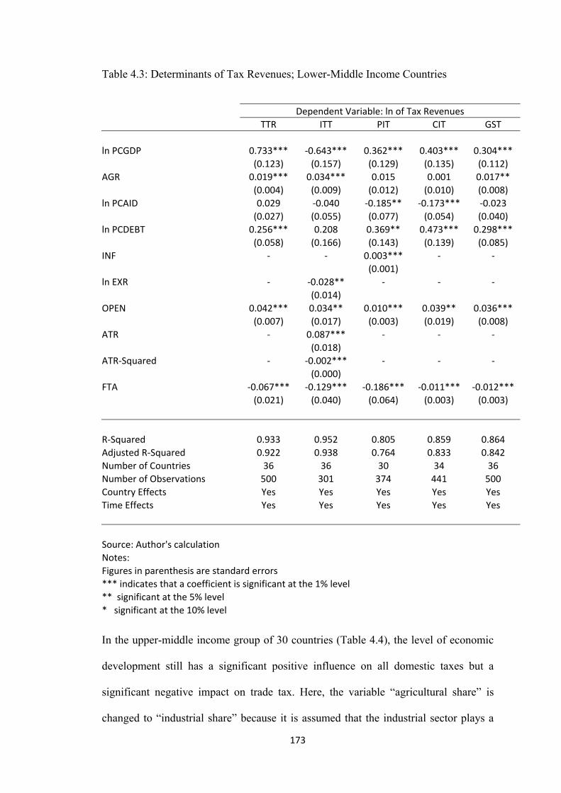
Table 4.3: Determinants of Tax Revenues; Lower-Middle Income Countries
Dependent Variable: ln of Tax Revenues TTR ITT PIT CIT GST ln PCGDP 0.733*** ‐0.643*** 0.362*** 0.403*** 0.304*** (0.123) (0.157) (0.129) (0.135) (0.112) AGR 0.019*** 0.034*** 0.015 0.001 0.017** (0.004) (0.009) (0.012) (0.010) (0.008) ln PCAID 0.029 ‐0.040 ‐0.185** ‐0.173*** ‐0.023 (0.027) (0.055) (0.077) (0.054) (0.040) ln PCDEBT 0.256*** 0.208 0.369** 0.473*** 0.298*** (0.058) (0.166) (0.143) (0.139) (0.085) INF ‐ ‐ 0.003*** ‐ ‐ (0.001) ln EXR ‐ ‐0.028** ‐ ‐ ‐ (0.014) OPEN 0.042*** 0.034** 0.010*** 0.039** 0.036*** (0.007) (0.017) (0.003) (0.019) (0.008) ATR ‐ 0.087*** ‐ ‐ ‐ (0.018) ATR‐Squared ‐ ‐0.002*** ‐ ‐ ‐ (0.000) FTA ‐0.067*** ‐0.129*** ‐0.186*** ‐0.011*** ‐0.012*** (0.021) (0.040) (0.064) (0.003) (0.003) R‐Squared 0.933 0.952 0.805 0.859 0.864 Adjusted R‐Squared 0.922 0.938 0.764 0.833 0.842 Number of Countries 36 36 30 34 36 Number of Observations 500 301 374 441 500 Country Effects Yes Yes Yes Yes Yes Time Effects Yes Yes Yes Yes Yes Source: Author's calculation Notes: Figures in parenthesis are standard errors *** indicates that a coefficient is significant at the 1% level ** significant at the 5% level * significant at the 10% level
In the upper-middle income group of 30 countries (Table 4.4), the level of economic
development still has a significant positive influence on all domestic taxes but a
significant negative impact on trade tax. Here, the variable “agricultural share” is
changed to “industrial share” because it is assumed that the industrial sector plays a
173

more important role in developed economies. The industrial sector is easier to tax than
the agricultural sector since businesses performing in the industrial sector usually
keep better accounts and records. In addition, products produced in this sector are
rarely exempt from the consumption tax. As expected, the coefficients for the share of
the industrial sector in GDP are statistically significant with a positive sign. Aid per
capita turns out to be negatively significant not only with income taxes, but also with
the consumption tax. This means that as these countries receive more aid, they have
less dependency on tax revenue, and hence there is a possibility that they use aid as a
domestic tax reduction since tax reduction is a tool that governments use to get more
vote and supporters for their next term (see for example Moore, 1998). The result is
inline with other studies such as that of Franco-Rodriguez, Morrissey, and
McGillivray (1998). The coefficient for debt per capita is positively significant for
income and goods and services taxes. This illustrates that upper-middle income
countries may choose to use domestic taxes as a mean of their debt payment. Inflation
still has a positive impact on personal income tax which illustrates the effect of
“bracket creep”. The coefficient for the exchange rates is negative and significant, in
line with the results of the other two income groups.
Increased trade openness again is observed to have led to an increase in the receipt of
all tax types, showing the high influence of the international trade sector in
determining tax collection. A potential “Laffer effect” exists for trade tax and the
revenue-maximizing rate of trade taxation, estimated to be 25%, is again higher than
the actual rate. The coefficients for free trade agreements are negative and significant
for all taxes, once again indicating that there is a harmful effect of trade liberalization
through trade agreement, not only on trade tax as usual, but also on domestic taxes.
174

Table 4.4: Determinants of Tax Revenues; Upper-Middle Income Countries
Dependent Variable: ln of Tax Revenues TTR ITT PIT CIT GST ln PCGDP 0.440*** ‐1.251*** 0.661*** 0.279*** 0.763*** (0.139) (0.160) (0.119) (0.085) (0.140) IND 0.014*** 0.001 0.058*** 0.037*** 0.023*** (0.004) (0.018) (0.023) (0.008) (0.007) ln PCAID ‐0.053*** ‐0.041 ‐0.098** ‐0.114*** ‐0.040** (0.017) (0.042) (0.046) (0.036) (0.021) ln PCDEBT 0.163*** ‐0.165 0.644*** 0.093** 0.291*** (0.065) (0.182) (0.148) (0.048) (0.055) INF ‐ ‐ 0.008*** ‐ ‐ (0.002) ln EXR ‐ ‐0.057*** ‐ ‐ ‐ (0.022) OPEN 0.014*** 0.036*** 0.020*** 0.100** 0.047*** (0.006) (0.011) (0.005) (0.046) (0.017) ATR ‐ 0.116** ‐ ‐ ‐ (0.053) ATR‐Squared ‐ ‐0.002** ‐ ‐ ‐ (0.001) FTA ‐0.032** ‐0.098*** ‐0.081** ‐0.057** ‐0.016** (0.015) (0.037) (0.039) (0.029) (0.008) R‐Squared 0.873 0.910 0.786 0.881 0.922 Adjusted R‐Squared 0.845 0.871 0.729 0.854 0.904 Number of Countries 30 29 27 28 30 Number of Observations 348 197 295 328 342 Country Effects Yes Yes Yes Yes Yes Time Effects Yes Yes Yes Yes Yes Source: Author's calculation Notes: Figures in parenthesis are standard errors *** indicates that a coefficient is significant at the 1% level ** significant at the 5% level * significant at the 10% level
For high income countries (Table 4.5), the coefficients for per capita GDP support the
hypothesis that a higher level of economic development is associated with a higher
use of complicated taxes and lower use of trade tax. The tax ratios, except for the
trade tax, are positively related to the share of the industrial sector in GDP, which
175

again reflects the greater ease of taxing the profits of industry rather than the income
from agriculture. The coefficient of inflation indicates that “bracket creep” exists
when there is higher inflation. Appreciation of currency leads to higher imports, and
hence higher trade tax.
For trade openness, although the coefficients are positive and significant for trade tax,
corporate income tax, and consumption tax, it is insignificant in raising total tax to
GDP. The level of economic development and the structure of the economy now seem
to matter. The result confirms Bahl’s (1971) comment that in developed economies,
trade tends to be less relevant than per capita income in determining the tax ratio.
Average tariff rates do not have a significant impact on trade tax, although the sign
shows that “Laffer effect” possibly occurs. Noticeably, while free trade agreements
have a significant negative impact on trade tax, similarly to the results of other
income groups, the coefficients for this variable are positive and significant for all
domestic taxes and total tax. This is interesting since the results indicate that while
low and middle income countries have to be careful in signing any trade agreement
because it may end up with the loss of tax revenue, high income countries, which
usually be the mainstay of urging other less developed countries to sign such
agreement, may benefit from trade agreement by gaining more tax revenue.
176

Table 4.5: Determinants of Tax Revenues; High Income Countries
Dependent Variable: ln of Tax Revenues TTR ITT PIT CIT GST ln PCGDP 0.622*** ‐0.706*** 0.762*** 0.723** 0.978*** (0.222) (0.268) (0.308) (0.346) (0.367) IND 0.013** ‐0.010 0.052*** 0.032*** 0.035** (0.006) (0.026) (0.012) (0.009) (0.015) INF ‐ ‐ 0.015** ‐ ‐ (0.007) ln EXR ‐ ‐0.900*** ‐ ‐ ‐ (0.262) OPEN 0.002 0.021*** 0.004 0.110** 0.052** (0.002) (0.008) (0.002) (0.054) (0.022) ATR ‐ 0.236*** ‐ ‐ ‐ (0.070) ATR‐Squared ‐ ‐0.004 ‐ ‐ ‐ (0.003) FTA 0.045** ‐0.022*** 0.048** 0.121*** 0.091*** (0.020) (0.008) (0.024) (0.021) (0.022) R‐Squared 0.923 0.982 0.883 0.902 0.927 Adjusted R‐Squared 0.914 0.973 0.868 0.891 0.919 Number of Countries 32 14 28 30 32 Number of Observations 632 129 552 588 629 Country Effects Yes Yes Yes Yes Yes Time Effects Yes Yes Yes Yes Yes Source: Author's calculation Notes: Figures in parenthesis are standard errors *** indicates that a coefficient is significant at the 1% level ** significant at the 5% level * significant at the 10% level
4.6. Conclusions
In research of trade liberalization, a lot of attention has been paid to its impact on
export performance, economic growth, employment, income distribution, and wage
inequality, but very little to its impact on taxation and government revenue. These are
equally important areas of inquiry, because if trade liberalization leads to a reduction
177

in tax revenues, this can have serious implications for fiscal reform of countries that
have a budget constraint. In other words, because trade liberalization is possibly
associated with a decrease in international trade tax revenue, if its negative impact is
spread on other domestic taxes, the suggesting solution using tax reform by replacing
trade tax with income or consumption taxes may be inefficient or even be
inapplicable. The sufferings from the loss of tax revenue may be much higher for
countries that have constrained government’s income sources, especially for most of
low and middle income countries which have a high dependency on trade tax revenue.
Dividing the estimation into four sub-samples including low, lower-middle, upper-
middle, and high income countries, the results of the analysis undertaken are strong
and robust to the estimation technique using two-way fixed effects, which means that
the conclusion can be presented with some confidence.
First, trade liberalization that leads to higher imports and exports has significantly
affected all taxes in low and middle income groups. The estimation has revealed the
important of the international trade sector in low and middle income countries’
economies. Openness to international trade obviously helps stimulate the collection of
income taxes, possibly by increasing employment, wage level, and corporate profits.
It also has a contribution to the consumption tax, possibly by spurring flows of goods
within the country. The positive relationship between the degree of trade openness
and trade tax means that openness possibly is a stimulus to higher volume of trade
between countries and consequently increases trade tax receipts at the current level of
the tariff rate. The effect of trade openness on both trade tax and domestic taxes
emphasizes the fact that, for low and middle income countries, not only is their trade
sector highly dependent on international sector, but also their entire economic
structure will be affected if there is any change in countries’ international trade
178

system. A change which leads to an increase in trade volume will consequently
benefit these countries’ taxation. By contrast, trade tends to be less relevant than per
capita income in determining tax revenue in high income countries. Thus, although
overall results suggest that trade liberalization via increasing trade openness generally
has a contribution to taxation in all countries, the degree of its benefit depends on the
country’s level of economic development and economic structure.
Second, there is an existence of the Laffer effect on trade tax in low and middle
income countries. From the estimated results, the actual tariffs are below the revenue-
maximizing rate, which in turn illustrates that a further reduction of tariff levels could
actually decrease trade tax revenue. This implies that trade liberalization in the form
of tariff reduction is harmful to countries where trade tax accounts for a high
proportion of their tax revenues.
Third, the impact of trade liberalization in the form of free trade agreements differs
according to the level of economic development. While free trade agreements have a
strong negative impact on all kind of taxes in low and middle income countries, they
seem to have a contribution to taxation in high income countries. The results raise
issues concerning agreements which are signed between developed and less
developed countries. Generally, many less developed countries are afraid of joining
any agreement with developed countries because most parts of their economic sector
are not well prepared for freer and higher competition, while developed countries,
which usually initiate such agreements, are believed to have a higher ability to take
advantages from those agreements. Their fear of trade liberalization is in line with
studies which suggest that freer trade may potentially lead to the fall in domestic
corporate profit, job loss, or even business shutdown. The negative impact of FTAs on
tax revenue may or may not result from the evidence suggested above. However, the
179

present results do suggest that the problem on taxation to be faced when entering free
trade agreements, especially in low and middle income countries, is a real one. Tax
reform suggested by economic theory and international experience by moving away
from international trade taxation and compensating the loss of trade tax by raising
more revenue from income and consumption taxes may be inapplicable since these
taxes also severely suffer from FTAs, not to mention the difficulties in improving
domestic tax administration which requires reorganizing along functional lines,
modernizing procedures, computerizing systems, and training people.
In conclusion, it should be stressed that because trade liberalization may take many
forms, its effects vary greatly in detail of liberalization. The results here do not imply
that trade liberalization in the form of FTAs is harmful to taxation since each
agreement differs in its detail. However, its negative impact is worth highlighting.
One policy conclusion from the results, therefore, would be that countries which need
to promote trade liberalization, especially for low and middle income countries, need
to take great care in every step of moving toward freer trade. Balancing the advantage
and disadvantage of trade liberalization may possibly help countries mitigate their
loss of trade tax revenue and achieve successful tax reform.
180

Appendix 4A: Summary of Previous Studies in Tax Effort
Table 4A1: Summary Table of Previous Studies in Tax Effort
Study Lotz and
Morss (1967)
Shin (1969) Bahl (1971) Tanzi (1992)
Piancastelli (2001) Teera (2002)
Alm, Martinez-
Varquez and Schneider
(2004)
Bahl (2003)
Sample Developing and Developed Countries
Developing and Developed Countries
Developing Countries
Developing Countries
Developing and Developed Countries
Developing and Developed Countries
Developing and Developed Countries
Less Developed Economies and OECD
Dependent Variable
Ratio of Tax Revenue to GNP
Tax Ratio Taxable Capacity
Tax Share Ratio of Total Tax Revenues to GDP
Tax to GDP Ratio
Ratio of Total Tax Revenues to GDP
Ratio of Tax Revenue to GDP
Independent Variables
GNP per capita
GNP per capita
Income per capita
Income per capita
GNP per capita
GDP per capita
GNP per capita
Sign + + + + + Mixed Results - Significance Significant
for full sample and low income countries, insignificant for high income countries
Significant for full sample
Insignificant Generally significant but insignificant for some years
Not always significant
Not always significant
Significant
Independent Variables
Ratio of imports plus exports to GNP
Foreign Trade Ratio
The Export Ratio
The Share of Imports in GDP
Ratio of Trade to GDP
Ratio of imports plus exports to GDP
Ratio of Openness
Sign + + + + + Both + and - + Significance Significant
for full sample and low income countries, insignificant for high income countries
Insignificant Not always significant
Significant Significant Positively significant for low and middle income countries, negative or insignificant for high income countries
Significant
Independent Variables
The Agricultural Income Ratio
The Agricultural Share
The Share of Agricultural sector in GDP
The Share of Agricultural sector in GDP
Ratio of Agriculture to GDP
Ratio of Agriculture to GNP
Sign - - - - Both + and - - Significance Insignificant Significant Significant Significant Negatively
significant for low income countries, positive and significant in some estimations for middle income countries
Insignificant
Independent Variables
The Mining Share
The Share of Industrial Sector in GDP
Ratio of Manufacturing to GDP
Ratio of Mining to GDP
The Non-Agricultural Share of GDP
Sign + + - + + Significance Significant Significant Insignificant Significant Significant Independent Variables
Level of Foreign Debt in GDP
The Share of Service Sector in GDP
Shadow Economy
Ratio of Shadow Economy to GDP
Sign + + + - Significance Not always
significant Not always significant
Not always significant
Significant
Independent Variables
Ratio of International Trade Tax to GDP
Sign - Significance Insignificant
181

Appendix 4B: Panel Unit Root Test
This study employs the Levin-Lin-Chu (LLC) test which is one of the first unit root
tests to be developed for panel data. The results in the table below indicate that there
is no presence of unit root. The LLC test rejects the null hypothesis of a unit root,
showing that all variables used in the study are stationary at level.
Table 4B1: The Panel Unit Root Test
Variables Full Sample Low
Income
Lower-
Middle
Income
Upper-
Middle
Income
High
Income
Taxes
lnTTR -6.11*** -7.74*** -9.15*** -7.42*** -8.53***
lnITT -7.84*** -17.95*** -5.81*** -9.16*** -13.04***
lnPIT -8.85*** -7.59*** -3.74*** -10.73*** -13.23***
lnCIT -3.96*** -1.97*** -5.07*** -4.50*** -3.31***
lnGST -7.87*** -7.02*** -4.75*** -9.71*** -4.35***
Independent
Variables
lnPCGDP -4.35*** -3.29*** -4.94*** -3.91*** -5.08***
AGR -2.51*** -2.93*** -2.26*** - -
IND -18.12*** - - -18.57*** -17.47***
lnPCAID -9.37*** -7.39*** -8.36*** -10.09*** -
lnPCDEBT -7.23*** -10.03*** -7.36*** -5.93*** -
INF -2.11*** -2.15*** -2.11*** -2.70*** -2.37***
lnEXR -5.10*** -4.62*** -2.47*** -7.27*** -4.71***
OPEN -3.69*** -3.57*** -4.41*** -2.03*** -3.63***
ATR -4.13*** -3.25*** -9.49*** -3.87*** -5.57***
ATR-
Square -6.97*** -7.36*** -6.77*** -5.62*** -8.68***
FTA -2.28*** -1.87*** -2.54*** -4.17*** -7.32***
The number in the table present Levin, Lin and Chu test statistics *** indicates the significance at 1% level
182

Chapter 5
The Impact of Trade Liberalization on
Revenue Mobilization and Tax Performance
183

5.1. Introduction
Trade liberalization is always considered as a potential source of fiscal instability
because it is usually associated with the decline in international trade tax revenue.
One of the critical issues about revenue related trade liberalization is that the boost to
international trade tax revenue from higher trade volume, as a consequence of tariff
reduction, will be insufficient to outweigh the revenue-dampening effect of tariff rate
reduction. Furthermore, in some cases, international trade tax revenue may be driven
down as a result of the reduction in international trade tax rates combined with the
weak expansion of it tax base. In order for a government to maintain fiscal stability
while liberalizing trade, an appropriate domestic tax reform must be performed. In
fact, in many programmes supported by the World Trade Organization (WTO),
substantial trade liberalization is suggested to be accompanied by comprehensive
domestic tax reform. More specifically, the loss of international trade tax revenue
should be compensated for by higher revenues from the taxation of domestic goods
and services and from direct taxes on income and profits.
The decrease in international trade tax revenue can be matched by an increase in
revenue from domestic indirect taxation. Keen and Ligthart (1999) suggest that a
combined tariff cut with a point-to-point increase in domestic consumption tax can
lead to an increase in public revenue. In particular, most countries have increased
reliance on Value-added tax (VAT), in which the VAT is suggested by many authors
to reduce the possibility of tax evasion and does not hurt the external competitiveness
of domestic producers. Value-added tax has been introduced in ASEAN countries,
with varying degree of success. VAT is introduced as part of an overall tax reform
during trade liberalization because it is administrated quite effectively and helped
boost fiscal revenue. However, in practice, the revenue performance of VAT and its
184
distributional effects will depend on the tax’s specific design and on the quality of its
administration. In addition, VAT tends to be less effective in developing countries
that have large informal sectors.
Considering the reform of tax administration itself, in the past, the lack of
administrative capacity reduces the efficiency of tax collection, while the large size of
the informal and subsistence sectors means that a large proportion of transactions
cannot be taxed. In addition, the influence of powerful lobbies makes some sectors
off-limits to the tax authorities. As a result the domestic tax base is narrow and a
government tries to meet its fiscal needs by charging high rates on easy-to-tax sectors
such as international trade (Kubota, 2000). Many recent studies suggest that one of
the keys to collect higher tax revenue is to improve tax administration. The main
problems of tax administration which are needed to be addressed include the lack of
financial and material resources, poorly trained staff, ineffective procedures, the
absence of effective taxpayer services, and corruption. To resolve these problems,
some countries has restructured their tax system, for example, by strengthening tax
administration, establishing tax monitoring units, improving audit practices, and
computerizing the tax system. Following these reforms, improving tax administration
could reduce tax evasion and consequently enhance fiscal revenue.
Generally, tax reform is an important instrument for raising tax yield. Usually, tax
productivity should be improved after the country reformed its tax system. However,
the effect of trade liberalization on the overall tax system is ambiguous. A positive
fiscal effect can arise if trade liberalization is accompanied by 1) a large expansion in
international trade volume which results in an increase in international trade tax, 2)
economic growth which later increases production, employment, and income level
and results in a larger base for personal and corporate income taxes, 3) devaluation of
185

the exchange rate which raises the domestic value of imports and hence stimulates
people to switch consumption from imports goods to domestic products and thus
increases goods and services tax base. By contrast, a negative fiscal effect can also
happen if trade liberalization is accompanied by shrinking trade volumes, job losses,
and deterioration in corporate profit. In addition, in principle, it is difficult to
determine the direction of change in tax revenue as a result of trade liberalization
because it depends crucially on revenue productivity and tax structure (Suliman,
2005). That is, growth in tax revenues may occur through automatic responses of the
tax yield through changes in national income and/or through the imposition of new
taxes, revision of the rate-structure of existing taxes, expansion of the tax bases, tax
amnesties, and tougher compliance and enforcement measures. Changes in tax yield
resulting from the modification of tax parameters (i.e., rates, base) are called
“discretionary changes” which stem from legislative action. Generally, tax buoyancy
and tax elasticity are the measures used to evaluate the ability of country’s tax system
to mobilize its revenue (Asher, 1989). Tax buoyancy measures the change in the
overall tax yield from changes in GDP whereas tax elasticity measures the change in
tax yield resulting from variations in national income with tax parameters held
constant (i.e., discretionary changes being removed).
In this chapter, a measure of revenue productivity of the tax system is used to
determine whether the responsiveness of tax revenues is high or low in Thailand
relative to three of the other founding countries of the ASEAN Free Trade Area
(Indonesia, Malaysia, and Philippines). By using the buoyancy and elasticity
framework, this chapter applies the concept of tax buoyancy and elasticity to evaluate
the implications of the process of trade liberalization on revenue mobilization. The
main objective of this chapter is to estimate tax buoyancy and tax elasticity of the tax
186
system of Thailand, compared to those of its three neighbour countries. The
evaluation is done to measure the response of the tax system to trade liberalization by
AFTA in 1992. More specifically, in this chapter we address the question of whether
Thailand’s major trade liberalization by becoming an AFTA member results in the
enhancement of the flexibility of the tax system. If there is any change or
improvement in Thailand’s tax system, which components of the tax structure have
been the most responsive, and why? If not, which tax sources have been rigid, and
why? What policy implications can be drawn? The results will be used for
comparison purpose in order to gain a wider perspective on the impact of AFTA on
the tax system among big ASEAN nations.
The rest of this chapter is divided into five sections. Section 2 gives details of taxation
choices in revenue from reforming income and consumption taxes discussed from a
theoretical perspective. This section also provides an overview of fiscal profiles of
Thailand and the other three ASEAN countries as well as the discussion on their fiscal
policies in order to identify any policy changes which occurred during the 1990s,
especially when countries joined AFTA. Section 3 reviews theoretical and empirical
studies on tax buoyancy and tax elasticity. Section 4 summarizes the methodology
and the data. Section 5 presents the empirical analysis. The final section gives some
summary and concluding remarks.
5.2. The Reform of Taxation in Developing Countries
In most developing countries, the major problem of the fiscal consequences of trade
liberalization is how to fit the revenue compensation into revenue loss from
liberalization. This area of concern involves domestic tax reform which is associated
with broad issues of economic policy, tax administration, and tax structure design.
187

Among the issues concerning tax reform, the most important and interesting point is
how to design the composition of tax structure. More specifically, the critical issue of
tax reform is how the government should design the major components of tax
structure to cooperate with trade liberalization in order to make the whole tax
structure desirable, administratively practicable, and politically feasible. Thus,
understanding fiscal backgrounds and fiscal policies of countries is a very necessary
step before tax reform is performed and evaluated. In addition, knowing which tax
handles should be used for domestic tax reform is crucial since it helps a government
to perform the reform efficiently.
Therefore, this section begins with the discussion on the main types of taxes that are
generally suggested to be used for tax reform. Then, the fiscal backgrounds and fiscal
policies in each of the four countries will be discussed to provide an insight of fiscal
movement of these four countries.
5.2.1. The Choice between Income and Consumption taxes: Theoretical
Considerations
This section begins with the choice between income tax and consumption tax, as a
tool for offsetting revenue shortfall as a consequence of trade liberalization. Although
the tax literature has traditionally suggested income tax as a preferred tool in raising
revenue, many recent works have emphasized a broad-based consumption tax as a
preferred source to mitigate the loss of revenue.36 The supporters of consumption tax
propose that the most attractive reason for using this tax source as a tool for revenue
offsetting is because consumption offers a large tax base for developing countries.
Moreover, the difficulties that arise with income tax administration are also the cases
36 See Auerbach (1996) and Jorgensen (1996) for example.
188

to avoid income taxes used for mitigation. However, another group has suggested that
reforming the tax system by focusing on consumption tax also encounters problems.
The modern concern proposed by Keen (2007) suggests that there is a failure in
applying the value-added tax (VAT) in some developing countries since the
administration of such a tax requires accurate accounting for financial transactions. In
general, central considerations in the debate of the reform focusing on income tax or
consumption tax are efficiency and equity, especially for developing countries which
usually have high inequality of income and wealth. For efficiency issue, the
theoretical literature has pointed out that taxing income is less efficient than taxing
consumption since it reduces higher welfare. Generally, income tax consists of two
broad components, a labour tax and a capital tax. On the part of labour tax, theory
suggests that taxing on labour wages causes additional distortions on savings while
consumption tax does not. On the part of capital tax, since capital can be divided into
physical capital and human capital, theory suggests that, although both taxing on
capital and taxing on consumption may have similar consequence by depressing
physical capital accumulation, capital tax may also have an additional impact on
human capital accumulation, which further lowers social welfare. Thus, when
considering efficiency, consumption tax is believed to be a more preferable tool for
raising revenue to offset the loss from trade liberalization. Another issue in the choice
between raising income tax and raising consumption tax involves the impact on
equity. This concern is particularly important in developing countries since there
usually is a highly uneven income distribution. The theoretical literature has
suggested that consumption tax is inherently more regressive than income taxes.
Taxing consumption is suggested to be ineffective in achieving equity objectives
because both the rich and the poor consume the same goods that are being taxed at the
189

same rate (though consuming in different proportions). Therefore, from the equity
point of view, raising revenue using income tax is preferable to raising revenue using
consumption tax. However, it is found that an application of consumption tax is
relatively feasible in practice and hence, is widely adopted by many developing
countries.
Since developing countries usually rely heavily on such convenient tax handles as
tariffs and import duties and count on these international trade taxes as an important
source of government revenue, lowering tariff rates in the process of trade
liberalization in order to join the World Trade Organization (WTO), to participate in
regional trading agreement such as AFTA or NAFTA, or to reach any bilateral trading
agreements with developed countries, could have a the significant impact on economy
and the government revenue of these countries. A significant loss in budgetary
revenue could possibly occur, at least in the short run before the volume of imports
respond to the changes in tariffs. As stated earlier, most developing countries have
decided to mitigate the loss under this circumstance by increasing domestic
consumption tax rather than increasing income tax since it is the most viable option
on grounds of both policy and administration. However, in order to determine
precisely the choice between income and consumption taxes, various aspects of these
tax handles should be discussed and compared. The following subsection highlights
some of the most important aspects of major tax handles used for mitigating the
revenue loss.
Personal Income Tax
In most developing countries, personal income tax (PIT) has yielded very little
revenue and thus is not counted as the most important tax handle in the tax structure
190

as it usually is in developed countries. This is mainly because there is a very small
number of individuals who are subject to PIT. In addition, administrative capabilities
are the major concerns in these countries. Cnossen and Bird (1990) provides a
comprehensive discussion on the PIT which highlights many interesting conceptual
issues.
Tax Rate
In general, the rate structure of the PIT in developing countries is not the primary
concern since many of these countries have maintained the progressivity of the PIT
tax rate by applying many rate brackets. Instead, the major concern is on tax
deduction, exemption, and credit which could severely affect the progression in the
rate structure. Cnossen and Bird (1990) suggest that in many developing countries, the
effectiveness of nominal rate progressivity in delivering effective rate progressivity is
substantial lowered by the high level of personal exemption. In particular, exemptions
and deductions in most cases are commonly found to benefit individuals with high
incomes. Such exemptions and deductions include the exemption of capital gain from
tax, the high deductions for medical and educational expenses, and the low taxation of
financial income. By reducing the number of rate brackets, exemptions, and
deductions, the effective rate progressivity of a country could be improved and,
therefore, the revenue raising objective together with an equity objective could be
achieved. In developing countries, it is also usually found that political constraints
impede the restructuring of PIT rates, a substantial improvement in PIT revenue
mobilization and in equity objective can also be achieved by replacing PIT deductions
with tax credits, which is equally beneficial for all tax payers in all tax brackets.
However, the use of tax credits accounts for a very little proportion in developing
countries.
191

Another important issue relating to PIT rate structure is the level of the top marginal
PIT rate. In some developing countries, this rate is almost equal or even exceeds the
corporate income tax (CIT) rate by a significant margin. This could drive taxpayers
from the PIT structure to the CIT form since various expense deductions in the CIT
structure provide a strong incentive for those taxpayers, which finally distort the tax
structure because the change does not generate from doing business purpose but
solely from tax purpose. Therefore, tax policy makers must be careful when choosing
to increase the PIT rate to offset the revenue loss from trade liberalization that the top
marginal PIT rate must be significantly lower than the CIT rate.
Tax Base
In addition to the problems of the high levels of exemptions and deductions that tend
to deteriorate the effective progressivity of a progressive nominal rate structure and
narrow the PIT base, most developing countries often encounter the problem of taxing
certain groups that have deficiency in coverage. Generally, these hard-to-tax groups
include small and medium enterprises, small and medium retail establishments, small
traders, professionals, and farmers, which are particularly important compositions in
developing countries. There are substantial difficulties in obtaining information on
their income. While data on earnings of employees in the public sector and in larger
private establishments are widely available, data for these hard-to-tax groups are not.
The computation of income tax based on their earnings or profit margins is very
difficult and hence requires other treatments than those provided by refined methods
of tax administration and provisions in the revenue code. However, the governments
of many developing countries are often reluctant to push these hard-to-tax groups into
the PIT structure since they do not want to lose political supports, as these groups are
accounted for a substantial proportion of the country’s population.
192
Corporate Income Tax
In developing countries, the issues which are related to tax reform by using CIT are
numerous and complex. Some of those issues are similar to those found in many
developed countries. However, this section focuses on two problematic issues which
are still prevalent in most developing countries; multiple CIT rates based on a sectoral
differentiation and tax incentives to promote investment.
Tax Rate
Generally, developing countries have a higher tendency to have multiple CIT rates
which are differentiated among sectors than that of developed countries. This includes
the exemption and deduction from tax of certain sectors. CIT rate differentiation in
most of developing countries is a result of past economic regimes which emphasize
the state’s role in resource allocation. There is an argument that multiple CIT rates
may distort the proper function of the market force. To address the distortion in the
sectoral allocation of resources, unifying multiple CIT rates across sectors is
suggested as an important tax policy in developing countries. However, unifying
multiple CIT rates may encounter a serious problem if the government chooses the
strategy to offset the revenue shortfall from trade liberalization by raising CIT rates
from sectors which reap benefit from the lower tariffs. This difficulty does not include
those sectors which have some kind of political power which may impede the strategy
to offset revenue shortfalls by using corporate income tax.
Tax Incentives
Although granting tax incentives to promote investment is quite common in countries
around the world, evidence suggests that it is particularly high for developing
193

countries. Investment incentives in developing countries are frequently given to both
domestic and foreign-owned businesses. Investment incentives may take various
forms, but among all the different forms of tax incentives, tax holidays and reduced
tax rates are the most popular among developing countries. There is an argument that
the revenue cost of tax incentives in the forms of tax holidays and reduced tax rates
are very high. In particular, tax incentives will be very costly if they are given to
businesses or sectors which benefit from lower import price as a result of tariff
reduction.
Goods and Services Tax
Goods and services tax usually plays a major part in the tax structure of developing
countries. The reason is very simple that goods and services tax is easier to impose
than income taxes. For collecting goods and services tax, fewer points of tax
collection are needed and taxation is concentrated on products either at the very first
stage of domestic manufacture or at various stages of production. In developed
countries, goods and services tax may be imposed as either a retail sales tax on
consumption or a value added tax of the consumption type by exempting capital
goods from the base. Where both options are available, the choice between them is a
matter of administrative convenience since the covered tax base and the burden
distribution will be the same. However, in developing countries, the retail option is
usually not available because the retail sector tends to be small, informal, and
unstable. The consequences are that sales cannot be determined accurately and
enforcement at the retail level is difficult. Therefore, most of developing countries
choose to go toward the value added approach since it is more feasible in practice. As
a result of its relative simplicity, developing countries usually implement domestic tax
reform by introducing the value added tax (VAT). However, it is usually found that
194

many important sectors in developing countries, including wholesale and service
sectors, have been left out of the VAT structure. In addition, the VAT credit
mechanism is still very restrictive, especially when it comes to provide tax credit to
for the capital goods. These problems greatly reduce the possibility of success when a
country chooses to introducing tax reform by focusing on goods and services tax.
5.2.2. Overview of Fiscal Profile
The four countries’ fiscal operations for the period 1972 to 2006 are highlighted from
Figures 5.1-5.4. All figures show that both government revenue and expenditure
maintained consistent growth patterns. In Figure 5.1, the graph shows that Thailand
suffered from a long-time deficit until 1988. Then, in the 1990s, revenue exceeded
expenditure until 1997, the year of the Asian economic crisis. During the crisis, there
was a drop in both revenue and expenditure, but a decrease was much larger for
revenue. From 1997, expenditure started to exceed revenue in absolute terms. In
addition, over the period 1991 to 2006, government revenue increased by 7.66% on
average compared with an increase of 9.80% in expenditure. Revenue started to
exceed expenditure again in 2003, although the gap between them was much lower
than that in the early 1990s period. Likewise, Indonesia and Malaysia had a huge
surplus in the second half of 1980s and the early 1990s. They also experienced a drop
in both revenue and expenditure in the Asian crisis period. They were able to maintain
a surplus from the second half of 1980s until now although the gap narrowed. By
contrast, the Philippines suffered from a deficit for almost the whole period, though
there was a little surplus during 1991-1996. From Figure 5.4, the deficit continued to
2006. Obviously, the deficit is can be traced from the economic crisis which occurred
in 1997. For most countries which have suffered the Asian financial crisis, including
these four countries, it was transformed to a full-blown recession in the real economy
195

of production. In order for the government to stimulate the domestic economy and
moderate economic recession, a large amount of government expenditure was utilized
for many years after the recession. Figures 5.1-5.4 point out that all four countries
need to boost revenue, especially for the Philippines, in order to prevent a fiscal
deficit which may potentially cause a rise in public debt and other fiscal problems in
the future.
Figure 5.1: Budgetary Revenues and Expenditures in Thailand, 1972 to 2006
0
10000
20000
30000
40000
50000
Total Revenue (US Dollar; Millions)
Total Expenditure (US Dollar; Millions)
Source: IMF the Government Finance Statistics (GFS); December, 2008
Figure 5.2: Budgetary Revenues and Expenditures in Indonesia, 1972 to 2006
0
10000
20000
30000
40000
50000
60000
70000
Total Revenue (US Dollar; Millions)
Total Expenditure (US Dollar; Millions)
Source: IMF the Government Finance Statistics (GFS); December, 2008
196
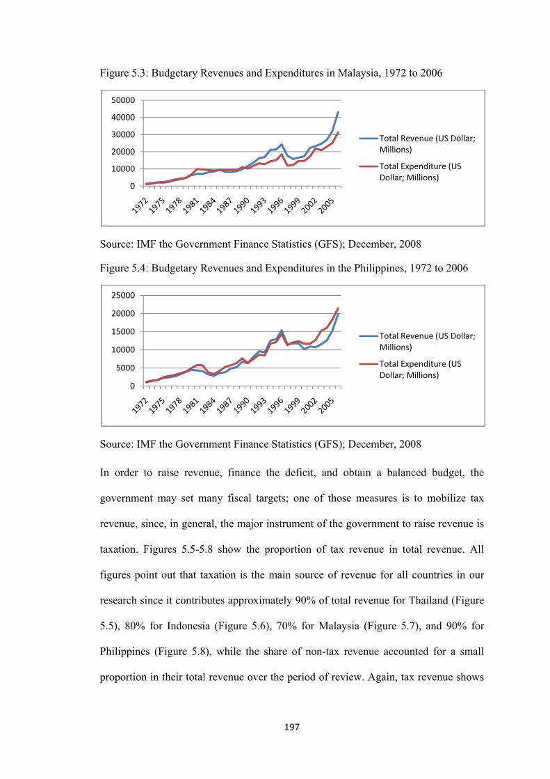
Figure 5.3: Budgetary Revenues and Expenditures in Malaysia, 1972 to 2006
0
10000
20000
30000
40000
50000
Total Revenue (US Dollar; Millions)
Total Expenditure (US Dollar; Millions)
Source: IMF the Government Finance Statistics (GFS); December, 2008
Figure 5.4: Budgetary Revenues and Expenditures in the Philippines, 1972 to 2006
0
5000
10000
15000
20000
25000
Total Revenue (US Dollar; Millions)
Total Expenditure (US Dollar; Millions)
Source: IMF the Government Finance Statistics (GFS); December, 2008
In order to raise revenue, finance the deficit, and obtain a balanced budget, the
government may set many fiscal targets; one of those measures is to mobilize tax
revenue, since, in general, the major instrument of the government to raise revenue is
taxation. Figures 5.5-5.8 show the proportion of tax revenue in total revenue. All
figures point out that taxation is the main source of revenue for all countries in our
research since it contributes approximately 90% of total revenue for Thailand (Figure
5.5), 80% for Indonesia (Figure 5.6), 70% for Malaysia (Figure 5.7), and 90% for
Philippines (Figure 5.8), while the share of non-tax revenue accounted for a small
proportion in their total revenue over the period of review. Again, tax revenue shows
197

a declining
even a high
trend durin
her level tha
ng the crisis
an that befor
s period but
re crisis, in
t it has risen
line with th
n back since
he trend of t
e the early 2
their total re
2000s to
evenue.
Figure 5.5
Millions); T
: Share of
Thailand, 19
f Tax and
972-2006
Non-Tax RRevenue inn Total Revvenue (US Dollar;
0
10000
20000
30000
40000
Source: IM
Figure 5.6
Millions); I
Source: IM
0100002000030000400005000060000
MF the Gove
: Share of
Indonesia, 1
MF the Gove
1972
1974
1976
1978
1972
1974
1976
1978
ernment Fin
f Tax and
1972-2006
ernment Fin
1980
1982
1984
1986
1980
1982
1984
1986
198
ance Statist
Non-Tax R
ance Statist
1988
1990
1992
1994
1988
1990
1992
1994
8
tics (GFS);
Revenue in
tics (GFS);
1994
1996
1998
2000
2002
1994
1996
1998
2000
2002
December,
n Total Rev
December,
2002
2004
2006
Non‐Tax R
Tax Reven
2002
2004
2006
2008
venue (US
2008
evenue
ue
Dollar;
Non‐Tax R
Tax Reven
evenue
ue

Figure 5.7
Millions); M
: Share of
Malaysia, 1
f Tax and
972-2006
Non-Tax RRevenue inn Total Revvenue (US Dollar;
0
10000
20000
30000
40000
50000
Source: IM
Figure 5.8
Millions); P
Source: IM
Considering
that trade l
trade tax re
accounted f
It ranked a
trade tax sh
1992 to 19
0
5000
10000
15000
20000
MF the Gove
: Share of
Philippines,
MF the Gove
g the impac
liberalizatio
evenue for a
for approxim
s the secon
hows a decli
997, the per
1972
1974
1976
1978
1972
1974
1976
1978
ernment Fin
f Tax and
, 1972-2006
ernment Fin
ct of trade l
on has been
all 4 countri
mately 25%
nd most imp
ining trend
riod that the
1980
1982
1984
1986
1980
1982
1984
1986
199
ance Statist
Non-Tax R
6
ance Statist
liberalizatio
n associated
ies. For Tha
% of total ta
portant tax s
over the pe
e country jo
1988
1990
1992
1994
1988
1990
1992
1994
9
tics (GFS);
Revenue in
tics (GFS);
on on tax re
d with a m
ailand (Figu
x revenue o
source until
eriod of stud
oined AFTA
1994
1996
1998
2000
2002
1994
1996
1998
2000
2002
December,
n Total Rev
December,
evenue, Fig
marked decli
ure 5.9), int
on average f
l 1991. Alth
dy, it drops
A. In 2006,
2002
2004
2006
2002
2004
2006
2008
venue (US
2008
gures 5.9-5.1
ine in inter
ternational t
from 1972 t
hough inter
very rapidly
internation
Non‐Tax R
Tax Reven
evenue
ue
Non‐Tax R
Tax Reven
Dollar;
evenue
ue
12 show
rnational
trade tax
to 1990.
rnational
y during
nal trade

tax accounted for only 8% of total tax revenue and ranked the least important among
major taxes in the country. Considering other taxes, goods and services tax ranked the
most important tax revenue source for Thailand. It accounted for approximately 50%
over the review period. Unlike the theory, goods and services tax does not show any
increasing trend to mitigate the loss of international trade tax over the liberalization
period. Instead, corporate income tax has risen since the late 1980s and become the
second most important tax in 2006. In 2006, corporate income tax accounted for more
than 30% of total tax revenue. Although the loss of international trade tax in Thailand
seems to be successfully mitigated, there are some concerns since corporate income
tax base is not as wide as the goods and services tax base. This may cause a problem
in raising revenue in the longer term.
Figure 5.9: Trends of Thailand’s Major Taxes
0
10
20
30
40
50
60
1972
1974
1976
1978
1980
1982
1984
1986
1988
1990
1992
1994
1996
1998
2000
2002
2004
2006
Personal Income Tax
Corporate Income Tax
Goods and Services Tax
International Trade Tax
Other
Source: IMF the Government Finance Statistics (GFS); December, 2008
For Indonesia (Figure 5.10), the international trade tax was about 20% of total tax
revenue in 1972 and has declined over the period. It accounted for approximately only
6% of total tax revenue in 2006. Like Thailand, the international trade tax was found
200

to be the least important tax source at the end of the period. Considering other taxes,
corporate income tax was considered to be the most important tax revenue source for
Indonesia during 1970s and 1980s since it accounted for over 50% of total tax
revenue on average. However, corporate income tax dropped rapidly in 1993 and the
revenue loss from corporate income tax was compensated by the rise of personal
income tax. In 2006, corporate income tax accounted for only about 8% of total tax
revenue, while personal income tax accounted for almost 40% of total tax revenue,
ranked the second most important tax revenue source for the country. In line with the
theory, goods and services tax shows an upward trend over the period of study. In
2006, it comprised almost 50% of total tax revenue and was the most important
source of tax revenue for the country.
Figure 5.10: Trends of Indonesia’s Major Taxes
0102030405060708090
1972
1974
1976
1978
1980
1982
1984
1986
1988
1990
1992
1994
1996
1998
2000
2002
2004
2006
Personal Income Tax
Corporate Income Tax
Goods and Services Tax
International Trade Tax
Other
Source: IMF the Government Finance Statistics (GFS); December, 2008
For Malaysia (Figure 5.11), the international trade tax shows a very obvious
downward trend over the period. In 1972, it is the most important tax revenue source
of the country by accounting for almost 40% of total tax revenue. However, its
proportion in total tax revenue dropped to approximately only 8% in 2006. At the end
of the study period, corporate income tax seems to play an important role for
201

government revenue since it made up approximately 50% of total tax revenue. The
goods and services tax does not show any increasing trend over the period as it
accounted for about 30%, ranked the second most important tax revenue.
Figure 5.11: Trends of Malaysia’s Major Taxes
0
10
20
30
40
50
60
1972
1974
1976
1978
1980
1982
1984
1986
1988
1990
1992
1994
1996
1998
2000
2002
2004
2006
Personal Income Tax
Corporate Income Tax
Goods and Services Tax
International Trade Tax
Other
Source: IMF the Government Finance Statistics (GFS); December, 2008
For Philippines (Figure 5.12), although international trade tax dropped rapidly after
the country joined AFTA, tax revenue from this source is still important for the
country since it was over 20% of total tax revenue in 2006, almost equal to the
proportion of corporate income tax and ranked the second most important tax revenue
source for the country. Although personal and corporate income taxes show an
upward trend, they grew very slowly, compared with other countries. The goods and
services tax does not seem to help mitigate the loss of international trade tax revenue
since it does not increase over time. From this fact, the Philippines may encounter a
severe problem if liberalization causes a significant reduction in international trade
tax revenue because there is no other taxes can help mitigate the loss.
202

Figure 5.12: Trends of Philippines’s Major Taxes
0
10
20
30
40
50
60
1972
1974
1976
1978
1980
1982
1984
1986
1988
1990
1992
1994
1996
1998
2000
2002
2004
2006
Personal Income Tax
Corporate Income Tax
Goods and Services Tax
International Trade Tax
Other
Source: IMF the Government Finance Statistics (GFS); December, 2008
From Figure 5.13 to Figure 5.16, Thailand’s data of tax revenues and per capita GDP
are plotted on the graph to demonstrate the relationship between them. Figure 5.13
shows that reliance on revenue from international trade tax is inversely related to the
country’s income levels. This fact is in line with the result in previous chapter. When
GDP is low, the country lacks administrative capacity, which reduces the efficiency of
tax collection. Government finds that it is difficult to tax the transaction of the
informal and subsistence sectors, which accounts for a large share in the country’s
economy. Additionally, the influence of powerful lobbies makes some sectors off-
limits to the tax authorities. As a result, the domestic tax base is narrow and the
government tries to meet its fiscal need by placing high rates on easily taxable sectors,
and one of those is on international trade (Kubota, 2000). However, as the country
grows, it relies less on the international trade tax and depends more on other domestic
taxes. While there is a decreasing trend in international trade tax against the income
level over the review period, taxes on income and profits increase with the level of
income. Figure 5.14 and Figure 5.15 show that taxes on income and profits are
positively associated with the country’s income level. From these two figures, it
203

seems that Thailand has tried to recover the loss of international trade tax by
collecting more income tax and profit tax, especially corporate income tax. However,
tax on goods and services does not show a clear relationship with the change in
income level. Figure 5.16 demonstrates that as the income changes, the goods and
services tax still remains at around 50% of total tax revenue and shows no increasing
trend as income increases.
Figure 5.13: Thailand’s reliance on international trade tax measured against income
levels, 1972-2006
0
5
10
15
20
25
30
35
40
2.4 2.6 2.8 3 3.2 3.4 3.6Revenu
e from
Internationa
l Trade
Tax
(percentage of Total Tax Reven
ue)
Log real per capita GDP
Source: IMF the Government Finance Statistics (GFS); December, 2008 and World Bank, World Development Indicators (WDI); December 2008
204

Figure 5.14: Thailand’s reliance on personal income tax measured against income
levels, 1972-2006
02468
101214161820
2.4 2.6 2.8 3 3.2 3.4 3.6Revenu
e from
Persona
l Incom
e Tax
(percentage of Total Tax Reven
ue)
Log real per capita GDP
Source: IMF the Government Finance Statistics (GFS); December, 2008 and World Bank, World Development Indicators (WDI); December 2008
Figure 5.15: Thailand’s reliance on corporate income tax measured against income
levels, 1972-2006
0
5
10
15
20
25
30
35
2.4 2.6 2.8 3 3.2 3.4 3.6Revenu
e from
Corpo
rate In
come
Tax
(percentage of Total Tax
Revenu
e)
Log real per capita GDP
Source: IMF the Government Finance Statistics (GFS); December, 2008 and World Bank, World Development Indicators (WDI); December 2008
205

Figure 5.16: Thailand’s reliance on goods and services tax measured against income
levels, 1972-2006
0
10
20
30
40
50
60
2.4 2.6 2.8 3 3.2 3.4 3.6Revenu
e from
Corpo
rate In
come
Tax
(percentage of Total Tax Reven
ue)
Log real per capita GDP
Source: IMF the Government Finance Statistics (GFS); December, 2008 and World Bank, World Development Indicators (WDI); December 2008
Figures 5.17-5.20 show the reliance of Indonesia’s major taxes on its income level.
Like the case of Thailand, Figure 5.17 shows that international trade tax is inversely
related to the country’s income level. As a country’s income grows, personal income
tax gradually increases, although it jumps up in later years when GDP reaches a high
level (Figure 5.18). However, unlike that of Thailand, corporate income tax does not
seem to mitigate the loss of international trade tax since it does not grow with the
country’s income (Figure 5.19). Still, there is a good sign for Indonesia since the
graph in Figure 5.20 shows that goods and services tax grows along with the
country’s income level. This implies that what really happens in practice is in line
with what the principle that loss of international trade tax revenue could be offset by
higher domestic consumption tax revenue. There is a chance to substitute domestic
consumption tax for international trade tax while maintaining government revenue for
Indonesia.
206

Figure 5.17: Indonesia’s reliance on international trade tax measured against income
levels, 1972-2006
0
5
10
15
20
25
2.2 2.4 2.6 2.8 3 3.2
Revenu
e from
Internationa
l Trad
e Tax
(percentage of Total Tax
Revenu
e)
Log real per capita GDP
Source: IMF the Government Finance Statistics (GFS); December, 2008 and World Bank, World Development Indicators (WDI); December 2008
Figure 5.18: Indonesia’s reliance on personal income tax measured against income
levels, 1972-2006
051015202530354045
2.2 2.3 2.4 2.5 2.6 2.7 2.8 2.9 3 3.1Revenu
e from
Internationa
l Trade
Tax
(percentage of Total Tax Reven
ue)
Log real per capita GDP
Source: IMF the Government Finance Statistics (GFS); December, 2008 and World Bank, World Development Indicators (WDI); December 2008
207

Figure 5.19: Indonesia’s reliance on corporate income tax measured against income
levels, 1972-2006
0102030405060708090
2.2 2.4 2.6 2.8 3 3.2
Revenu
e from
Internationa
l Trad
e Tax
(percentage of Total Tax
Revenu
e)
Log real per capita GDP
Source: IMF the Government Finance Statistics (GFS); December, 2008 and World Bank, World Development Indicators (WDI); December 2008
Figure 5.20: Indonesia’s reliance on goods and services tax measured against income
levels, 1972-2006
0
10
20
30
40
50
60
2.2 2.3 2.4 2.5 2.6 2.7 2.8 2.9 3 3.1Revenu
e from
Internationa
l Trade
Tax
(percentage of Total Tax Reven
ue)
Log real per capita GDP
Source: IMF the Government Finance Statistics (GFS); December, 2008 and World Bank, World Development Indicators (WDI); December 2008
Figures 5.21-5.24 show the relationship of Malaysia’s major taxes and its income
level. As shown by Figure 5.21, international trade tax is, again, negatively related to
the country’s income level. For Malaysia, Figures 5.22 and 5.23 show that personal
208
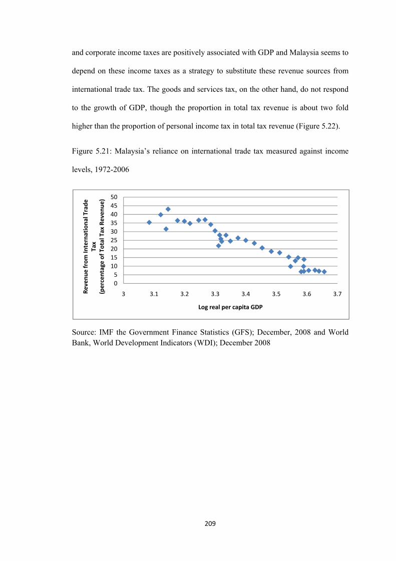
and corporate income taxes are positively associated with GDP and Malaysia seems to
depend on these income taxes as a strategy to substitute these revenue sources from
international trade tax. The goods and services tax, on the other hand, do not respond
to the growth of GDP, though the proportion in total tax revenue is about two fold
higher than the proportion of personal income tax in total tax revenue (Figure 5.22).
Figure 5.21: Malaysia’s reliance on international trade tax measured against income
levels, 1972-2006
05
101520253035404550
3 3.1 3.2 3.3 3.4 3.5 3.6 3.7Revenu
e from
Internationa
l Trade
Tax
(percentage of Total Tax Reven
ue)
Log real per capita GDP
Source: IMF the Government Finance Statistics (GFS); December, 2008 and World Bank, World Development Indicators (WDI); December 2008
209

Figure 5.22: Malaysia’s reliance on personal income tax measured against income
levels, 1972-2006
02468
1012141618
3 3.1 3.2 3.3 3.4 3.5 3.6 3.7Revenu
e from
Internationa
l Trade
Tax
(percentage of Total Tax Reven
ue)
Log real per capita GDP
Source: IMF the Government Finance Statistics (GFS); December, 2008 and World Bank, World Development Indicators (WDI); December 2008
Figure 5.23: Malaysia’s reliance on corporate income tax measured against income
levels, 1972-2006
0
10
20
30
40
50
60
3 3.1 3.2 3.3 3.4 3.5 3.6 3.7
Revenu
e from
Internationa
l Trade
Tax
(percentage of Total Tax Reven
ue)
Log real per capita GDP
Source: IMF the Government Finance Statistics (GFS); December, 2008 and World Bank, World Development Indicators (WDI); December 2008
210

Figure 5.24: Malaysia’s reliance on goods and services tax measured against income
levels, 1972-2006
0
5
10
15
20
25
30
35
40
3 3.1 3.2 3.3 3.4 3.5 3.6 3.7Revenu
e from
Internationa
l Trade
Tax
(percentage of Total Tax Reven
ue)
Log real per capita GDP
Source: IMF the Government Finance Statistics (GFS); December, 2008 and World Bank, World Development Indicators (WDI); December 2008
Figures 5.25-5.28 present the reliance of Philippines’s major taxes on its income
level. Similar to other three countries, international trade tax is inversely related to the
income level, as shown in Figure 5.25. However, as presented by Figures 5.26 and
5.28, personal income and goods and services taxes do not increase as income
increases. The only major tax of Philippines that grows with its GDP is corporate
income tax (Figure 5.27). This may raise concerns of how the Philippines’s
government will coordinate tariff and tax reform while maintaining government
revenue.
211
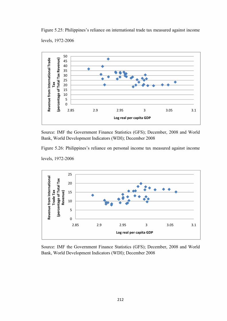
Figure 5.25: Philippines’s reliance on international trade tax measured against income
levels, 1972-2006
05
101520253035404550
2.85 2.9 2.95 3 3.05 3.1Revenu
e from
Internationa
l Trade
Tax
(percentage of Total Tax Reven
ue)
Log real per capita GDP
Source: IMF the Government Finance Statistics (GFS); December, 2008 and World Bank, World Development Indicators (WDI); December 2008
Figure 5.26: Philippines’s reliance on personal income tax measured against income
levels, 1972-2006
0
5
10
15
20
25
2.85 2.9 2.95 3 3.05 3.1
Revenu
e from
Internationa
l Trad
e Tax
(percentage of Total Tax
Revenu
e)
Log real per capita GDP
Source: IMF the Government Finance Statistics (GFS); December, 2008 and World Bank, World Development Indicators (WDI); December 2008
212

Figure 5.27: Philippines’s reliance on corporate income tax measured against income
levels, 1972-2006
0
5
10
15
20
25
2.85 2.9 2.95 3 3.05 3.1Revenu
e from
Internationa
l Trade
Tax
(percentage of Total Tax Reven
ue)
Log real per capita GDP
Source: IMF the Government Finance Statistics (GFS); December, 2008 and World Bank, World Development Indicators (WDI); December 2008
Figure 5.28: Philippines’s reliance on goods and services tax measured against
income levels, 1972-2006
0
10
20
30
40
50
60
2.85 2.9 2.95 3 3.05 3.1Revenu
e from
Internationa
l Trade
Tax
(percentage of Total Tax Reven
ue)
Log real per capita GDP
Source: IMF the Government Finance Statistics (GFS); December, 2008 and World
Bank, World Development Indicators (WDI); December 2008
213

5.2.3. Summary of Fiscal Policies
This section provides direction of fiscal policies and identifies policy changes under
the implementation of tax reform following trade liberalization in each of the four
countries. Generally, in performing domestic tax reform, the government expects an
improvement in the quality of the tax structure by emphasizing the country’s tax
potential in order to establish fiscal sustainability and increase the level of the
country’s tax competence both for the transition period of trade liberalization and in
the long term. In offsetting the revenue loss from trade liberalization, domestic tax
reform increases the opportunity to raise national revenue without increasing rates by
either increasing the capacity of tax administration, or expanding tax bases or both.
The reason is that, particularly for less developed and developing countries, there is
still room for improvement since the utilization of both tax administration and tax
bases are far from up to capacity. Therefore, this section is dedicated to discuss fiscal
policies in each of the four countries implemented in line with domestic tax reform
which is undertaken in the period of trade liberalization (the period of joining AFTA,
in particular) in order to investigate how the selected countries have attempted to
achieve the objective of revenue loss mitigation.
5.2.3.1. Thailand’s Tax Reform
Since the first Economic and Social Development Plan was introduced in 1961 in
order to promote industrial development and pursue an import substitution strategy,
the tax structure has been simultaneously adjusted and fine-tuned to enhance
effectiveness and efficiency of tax administration. However, from the 1960s to 1980s,
there was no major change in the country’s tax framework. It was not until the early
1990s that the government started thoroughly to review its tax system. The 1990s was
214

a period of substantial development and there was a dramatic change in global trend.
There was a large increase in international trade, investment, and factor mobility.
Trade policies have been changed from import substitution to export orientation and
protectionism has been gradually reduced. More social and economic cooperation has
been established in the region such as Asia-Pacific Economic Cooperation (APEC)
and ASEAN Free Trade Area (AFTA) which are mainly aimed to spur trade
liberalization in the Asian region. In order to integrate Thailand into the world
economy, a trade liberalization policy has been adopted and thus tax reform policies
have been used to mitigate the potential revenue loss from tariff reduction and to
enhance the productivity of the tax system as a whole.
Since the early 1990s, Thailand has implemented economic reform in various areas
including public, financial, and fiscal sectors. As part of overall fiscal reform, the
Thai government has implemented major domestic tax reforms, marked by the
introduction of the value added tax (VAT) and other tax reform measures starting in
1992. The rationale of domestic tax reform is twofold. Firstly, tax reform is a part of
changes in tax structure to offset any revenue loss from tariff reduction. By this
means, the Thai government has attempted to substitute revenue sources from tariffs
and custom duties to income and consumption taxes, reducing the dependency on
international trade tax and focusing to generate more revenue from domestic tax
bases. Secondly, tax reform is implemented to increase the efficiency in revenue
generation in a reasonably non-distorting, equitable, and sustainable manner.
The major composition of government revenue comprises personal income tax,
corporate income tax, value added tax, import duties, and excise tax. In Thailand, tax
revenue is collected through three departments, namely the Revenue Department, the
Excise Department, and the Custom Department. These three departments work under
215

the authority of the Ministry of Finance. The Revenue Department is responsible for
the collection of personal income tax, corporate income tax, value added tax, special
business tax, petroleum tax. The Excise Department is responsible for the collection
of tobacco tax, liquor tax, automobile tax, and other selected excise tax. The Custom
Department is responsible for the collection of import and export duties. Among the
three departments, the Revenue Department is the most important tax collection
department since the revenue collected by this department comprises approximately
70% of total tax revenue.
Major tax reforms which have been undertaken since the 1990s focus not only on
import duties, income taxes, and consumption tax, but also on tax administration.
Detail of the reform are given below.
Comprehensive Reform of the Custom Tariff Structure
In Thailand, custom duties are levied on both imports and selected exports. Duties are
levied on either a specific or an ad valorem basis depending on which one is higher.
In 1985, Thailand’s average tariff rate was over than 40%, with the highest rate being
for passenger cars in which the rate is over than 80%. However, as the country joined
free trade agreement as AFTA and trade liberalization programme provided by the
WTO, tariff rates have recently been reduced to the target range of three rates in
accordance with the production processes. The target rates are 1% for raw materials
and inputs which are not locally produced, 5% for semi-finished products, and 10%
for finished products, products requiring extra protection, and luxury goods. Although
the reform package has not yet been completed for all products, a number of products
in most categories have already adjusted to the new rates. Remaining items are such
as petrochemical products in which their tariffs rate will be reduced in line with the
216
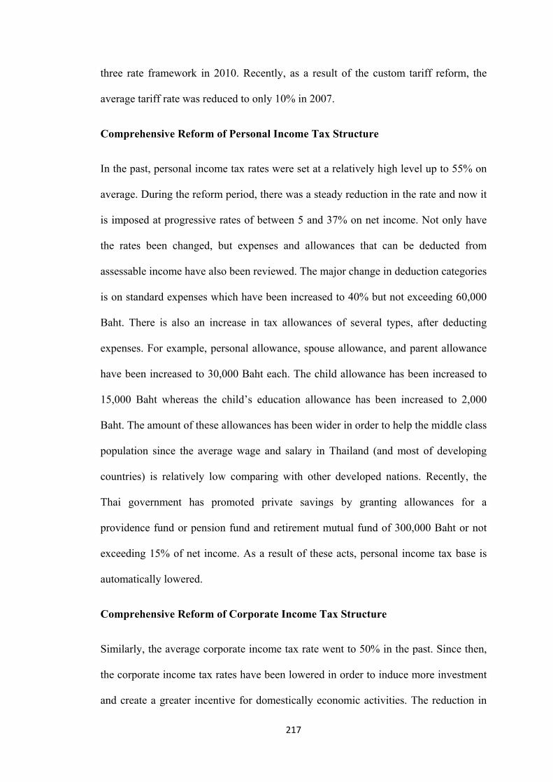
three rate framework in 2010. Recently, as a result of the custom tariff reform, the
average tariff rate was reduced to only 10% in 2007.
Comprehensive Reform of Personal Income Tax Structure
In the past, personal income tax rates were set at a relatively high level up to 55% on
average. During the reform period, there was a steady reduction in the rate and now it
is imposed at progressive rates of between 5 and 37% on net income. Not only have
the rates been changed, but expenses and allowances that can be deducted from
assessable income have also been reviewed. The major change in deduction categories
is on standard expenses which have been increased to 40% but not exceeding 60,000
Baht. There is also an increase in tax allowances of several types, after deducting
expenses. For example, personal allowance, spouse allowance, and parent allowance
have been increased to 30,000 Baht each. The child allowance has been increased to
15,000 Baht whereas the child’s education allowance has been increased to 2,000
Baht. The amount of these allowances has been wider in order to help the middle class
population since the average wage and salary in Thailand (and most of developing
countries) is relatively low comparing with other developed nations. Recently, the
Thai government has promoted private savings by granting allowances for a
providence fund or pension fund and retirement mutual fund of 300,000 Baht or not
exceeding 15% of net income. As a result of these acts, personal income tax base is
automatically lowered.
Comprehensive Reform of Corporate Income Tax Structure
Similarly, the average corporate income tax rate went to 50% in the past. Since then,
the corporate income tax rates have been lowered in order to induce more investment
and create a greater incentive for domestically economic activities. The reduction in
217

the corporate income tax rate is in line with the global trend for lowering tax rates.
Currently, corporate income tax is set at 30% on net profit for all types of businesses.
However, further reduced rates are also applied depending on the type of businesses.
These reduced rates have been recently used as policy instruments to promote certain
sectors such as Small and Medium Enterprises (SMEs) and listed companies. These
acts, on one hand, automatically reduce the collection by lowering the tax rate, but on
the other hand, may help improve the corporate income tax base by including more
businesses into the tax structure.
Comprehensive Reform of Goods and Services Tax Structure
One of the most important tax reforms in recent Thai history is the introduction of the
value added tax (VAT) in 1992 as a replacement for the business tax. After the VAT
was implemented, products that were liable for higher tax amount under the business
tax such as electrical appliances, automobiles, perfume and cosmetics were taxed at
the normal VAT rate and higher excise tax, leaving the tax burden remains
unchanged. The VAT is a tax on total consumption expenditure in which the burden is
purely on consumers. The VAT is charged at a single rate of 7%.
Comprehensive Reform of Tax Administration
Together with the reform in the structure of taxation, the tax administration has also
been substantial improved during the 1990s. The most important reform is the
introduction of online processing and the use of web base technology. In the past, the
process of tax collection was time consuming. By introducing information and
communication technologies, the working process has been largely shortened. The tax
database, data processing system, tax supervision system, and supporting system have
also been improved. These actions help improving up-to-date taxpayer information,
218

enhancing voluntary compliance, lowering debt delinquency, increasing taxpayer’s
cooperation, and consequently increasing the amount of tax collection.
5.2.3.2. Malaysia’s Tax Reform
Recently, the Malaysian government has faced the real challenge to assure its fiscal
sustainability due to the decline of revenue from tariff reduction. At the same time,
the government has attempted to lessen the budget reliance on international trade tax
and to depend more on domestic taxes. Besides increasing the efficiency of
expenditure, on the revenue side, the Malaysian government has no other choice but
effectively to mobilize domestic taxes because they have a great potential to be the
main source of government funding. Although there are many way to mobilize tax
revenue, including increasing tax rates, expanding tax bases, and improving tax
administration, the Malaysian government tends to choose to increase national
revenue by the process of tax reform without having to increase tax rates. The major
objectives for the reform in Malaysia’s tax system are to simplify the tax system, to
modernize the tax administration, to introduce various incentives to promote
investment, to introduce tax reliefs to reduce the tax burden of the lower income
group, to improve the investment climate, to promote domestic consumption, to foster
a caring society, and to enhance R&D and skill training.
Unlike many other countries which adopted the reform package that provides major
tax changes in the tax reform, Malaysia has also taken the incremental approach
which consists of a series of small steps of tax changes. The reform was undertaken
gradually and easy to manage by the tax authorities as well as to be withdrawn if
unpopular. However, the most notable tax reform of Malaysia’s tax system is the
introduction of the self-assessment system done in 1992. At that time, the Malaysian
219
government found that there is an opportunity to mitigate the loss of tariff revenue by
increasing capacity in personal income tax. The government has also realized that
there should have a better system for tax administration to deal with the increasing
number of taxpayers without a proportionate increase in the number of staff of tax
authorities. Self assessment is not a new tax but it is a system in which tax payers
must determine their own tax liabilities and make a payment accordingly. Along with
the self assessment system, there is an enhancement in ICT capabilities in order to
capture and update tax payers’ information and to improve audit and investigation
management.
5.2.3.3. Indonesia’s Tax Reform
Tax revenue is a main source of income for Indonesia. The country’s tax system is
based on personal income tax and value added tax system. The main difference that
distinguishes Indonesia’s tax system from the others is its relatively small dependence
on international trade tax over time. With limited dependence on international trade
tax, trade reform under trade liberalization regime has only a moderate impact on
government revenue. However, what seems to be a serious problem is the potential of
corporate income tax collection, especially once oil and gas revenues have been
removed. Since the 1980s, the proportion of oil and natural gas tax revenues has
gradually decreased from almost 80% to approximately only 10% in corporate income
tax. Since then, corporate income tax has experienced a substantial decrease and thus
a reform is needed to improve the efficiency of corporate income tax collection.
Therefore, the need to implement tax reform in Indonesia is not only raised from trade
liberalization perspective, but also from a business competitiveness perspective.
Therefore, the Indonesian government has set two main objectives for reforming the
220

country’s tax structure. With a more integrated world economy, Indonesia has to walk
into the process of trade liberalization, both in regional and world trade. Tax reform
must be done to mitigate the loss in tariff revenue, which used to be one of the main
sources of the country’s revenue. Tax reform must also help improve the investment
climate in order to attract more investors, both domestic and foreign ones, to put their
portfolio in the country.
Reform of Personal Income Tax
Personal income tax in Indonesia is subject to a five-bracket progressive rate, ranging
between 5% and 35%. Most of individual taxpayers are permanent workers and pay
their tax by wage withholding. Only a few proportions of taxpayers pay their income
tax by self assessment. Since the potential of the personal income tax system has been
great for decades, there was no significant personal income tax reform during the
1990s. However, there is an improvement in computer system over time to investigate
and assess individual taxpayers.
Comprehensive Reform of Corporate Income Tax
Except for the decrease once gas and oil revenues are removed from its structure, the
amount of revenue collected from the corporate income tax is relatively low compared
with other taxes. The very low collection is mainly due to Indonesia’s corporate
structure in which over 90% of Indonesian industry corporate is dominated by small
and medium enterprises where most of them are not legal entity and hence are not tax
registration companies. In addition, most of these businesses are retailers and
agricultural businesses which have a high tendency of tax evasion. The possibility of a
tax base expansion, although very difficult, is necessary since these small and medium
enterprises largely dominate the corporate structure and make a great contribution to
221

Indonesian GDP. The reform is aimed to include these companies into the corporate
income tax base but the expected time frame to collect majority of revenue from these
sources is in the medium term.
Comprehensive Reform of the VAT
In Indonesia, VAT is imposed with a single rate at 10% and is levied on a broad base
of goods and services. After implementation of tax reform in the early 1990s, various
tax policy measures related to VAT have been changed to improve the revenue
productivity of VAT including the reduction of VAT exemptions, the removal of the
zero rate VAT except for exports, the abolishment of the exemption on government-
borne VAT on certain goods, and the collection on most food products except basic
goods consumed by the poor and certain strategic goods including agriculture. The
government has also strengthened the VAT structure by expanding the base to, for
example, mining and hotels. A substantial improvement in tax administration,
particularly by introducing new technologies, was also achieved in the 1990s period.
5.2.3.4. Philippines’s Tax Reform
In the past, the Philippines tax system was not very strong and buoyant. The
inefficiency of the overall tax structure forced the country to be highly dependent on
such international trade tax as import tariffs. As a result of the absence of tax
productivity, many infrastructures were not constructed, public utilities deteriorated,
and health services remained inadequate. Although the Philippines’ government has
privatized its assets and borrowed heavily to finance the budget deficit, these
measures have provided only a temporary solution in the short and medium terms but
could not guaranteed the long-term fiscal stability for the country. Together with
globalization and the upward trend of free trade around the world, Philippines has
222

automatically been forced to reduced its high dependency on international trade tax.
Thus, in order to maintain its fiscal position and to create a productive and consistent
tax structure, comprehensive tax and tariff reforms were introduced in March 1992, in
line with the AFTA membership.
As goods and services tax is the highest performer among all tax types, the
Philippines’ government has focused tax reform on personal and corporate income
taxes. In implementing income tax reform, the Philippines’ government has aimed to
generate more tax revenue by simplifying the tax system in order to encourage greater
compliance from taxpayers, including those in the underground economy, removing
areas of discretion which provides avenues for tax avoidance and abuse, broadening
the tax base by investigating undeclared revenues and hidden taxpayers, improving
the taxation of the hard-to-tax income, reducing exemptions to enhance the amount of
revenue, and strengthening the enforcement of laws. The most significant reform in
the personal income tax structure is the use of residence instead of citizenship as a
basis for taxation. In order to solve the problem of tax avoidance, tax brackets have
been broadened so that additional wages or earnings would be subject to the same tax
rate and not to a higher marginal tax rate. On the other hand, in order to raise
corporate income tax revenue, the Philippines government needs to push more SMEs
into the tax structure. In order to achieve this goal, the corporate tax rate has been
gradually reduced. The Philippines government has also broadened the base of the tax
system by instituting control on deductible expenses which are often subject to the
discretion of the taxpayer and tax examiner. Such discretion can potentially lead to
abuses and tax avoidance practices which finally result in the leakages and loopholes
in the corporate income tax system.
223

5.3. General Review: Buoyancy and Elasticity of Tax Revenue and Empirical
works on Revenue Productivity of the Tax System
In order for a government to plan properly how to mitigate the loss in trade tax
revenues by substituting trade taxes to other domestic taxes, it is important to be able
to estimate tax buoyancy, built-in tax elasticity, and the impact of discretionary
changes on tax revenues. In fact, the estimation of the responsiveness of tax revenues
has long been a central empirical issue in applied public economics. The concepts of
tax buoyancy and tax elasticity are very important in the study of modern taxation
(Mansfield, 1972). Tax buoyancy and tax elasticity are usually used to measure tax
productivity. They measure the responsiveness of tax yield to changes in national
income. In general, changes in tax revenues are caused by automatic responses of tax
yield through national income changes and discretionary changes. Discretionary
changes are normally legislative actions done by the government such as the
imposition of new taxes, revision of existing tax rates, expansion of tax bases,
modification of tax amnesties, and enforcement of new measures. By concepts, tax
buoyancy measures the relationship between historical tax revenue and national
income in terms of proportional increase in tax revenue following a one percent
change in national income. On the other hand, tax elasticity measures relationship
between tax revenue at a constant tax structure and national income. If there is no
change in tax parameters (i.e., tax rates, tax base) during the reference period,
buoyancy will be same as elasticity. In other words, elasticity of tax is the rate of
proportionate change in the tax revenue due to change in national income while tax
buoyancy is the composite of the change in tax revenue due to change in national
income and discretionary tax changes.
224

However, the estimation of tax elasticity has suffered from a specification bias which
results from the unavailability of data. Ehdaie (1990) states that the lack of “an
observable quantitative variable” which is capable of reflecting all changes in an
individual (or overall) tax system, has a great impact on the accuracy of the
estimation. Because such necessary data as the effective tax rates and the changing
composition and growth of tax base are usually not available in most countries, the
need for a method for adjusting the historical tax series for discretionary changes has
arisen. Until recently, there are two widely used adjustment methods in the literature;
which are the proportional adjustment method and the dummy variable method. Both
methods will be described in the following topics.
Proportional Adjustment Method
The proportional Adjustment (PA) Method is used to eliminate the discretionary
effects from the revenue series. This method is usually attributed to many sequential
studies including Prest (1962), Mansfield (1972), Bahl (1972), and Chelliah and
Chand (1974). Based on the procedure proposed by Mansfield (1972), the
proportional adjustment method for computing tax elasticity involves a three-step
process. First, a preliminary series of adjusted tax yields is obtained by subtracting the
budgetary estimates of the effects of discretionary tax changes from the actual tax
yield, that is,
,t t t tT T D= − (5.1)
where;
,t tT is the adjusted or cleaned tax yield in the tth year
tT is the actual tax revenue yield in the tth year
225

tD is the budget estimate of the yield arising out of discretionary tax changes in the tth
year
Second, this preliminary series ( ) is further adjusted to exclude the continuing
impact of each discretionary change on all future years’ tax yields by multiplying by
the ratio of the previous year’s adjusted figure to the actual tax receipt. It can be
shown that this procedure involves a factor sequence, each element of which
represents the effect of the automatic component of tax changes in earlier years.
These two steps constitute the ‘data cleaning’ process, that is,
,t tT
1 1,1
12 2
1
23 3
2
1,
1
( )
( )( )
( )( )
( )( ) tt t
t
T T
TT TT
TT TT
TT TT
−
−
′ =
⎡ ⎤′′ = ⋅⎢ ⎥
⎣ ⎦⎡ ⎤′
′ = ⋅⎢ ⎥⎣ ⎦
⎡ ⎤′′ = ⋅⎢ ⎥
⎣ ⎦
M
,2
,3
t
Through sequential substitution, it can be shown that the above formula can be
rewritten in terms of and as; tT s tD s
1
1
( ) ( )t
j jt t t
j j
T DT T D
T
−
=
⎡ ⎤−′ = − ⎢
⎢ ⎥⎣ ⎦∏ ⎥ (5.2)
which is Mansfield core equation for proportional adjustment data cleaning.
Third, the resulting series of ‘cleaned’ tax yields is then regressed on some measure of
the tax base to obtain the necessary elasticity values.
However, using the proportional adjustment method is likely to cause bias in the
estimation. The essential weakness of the proportional adjustment method lies in the
data cleaning procedure. It is asserted that this procedure yields a series which is
226

systematically biased, and will therefore lead to biased elasticity estimates. Thus, the
proportional adjustment method, as commonly used, will almost always yield biased
estimates of the tax elasticity.37
For example on empirical study done when estimating the tax elasticity by using
proportional adjustment approach, Mansfield (1972) estimates tax buoyancy and tax
elasticity of Paraguay’s tax system from 1962 to 1970 to analyze the growth of
revenue. In his study, tax buoyancy and tax elasticity of Paraguay’s tax system are
calculated to be 1.69 and 1.14, respectively. Both coefficients for buoyancy and
elasticity are also estimated and compared for major taxes including income tax,
wealth taxes, and import taxes. Then, tax elasticities are decomposed into tax-to-base
elasticities and base-to-income elasticities in order to compare the growth rates. From
the results, he concludes that discretionary changes in the country’s tax system
primarily lead to a substantial increase in the tax ratio over the period of study. The
improvement of tax-to-base elasticities is necessary for the country to obtain more tax
yield. A more recent study, Muriithi and Moyi (2003), analyzed the productivity of
Kenya’s overall tax system and its major taxes, including direct taxes, import duties,
excise duties, and sale tax and VAT, after the tax structure was modernized in 1986.
In general, it is assumed that the tax yield or productivity should be improved after a
country’s tax system is reformed. Taking the analysis over the period 1973 to 1999,
the study estimates before- and after-reform buoyancy and elasticity, and then
compared the flexibility. They conclude that tax reform improves the response of tax
revenue to both the automatic changes in GDP and the discretionary tax measures,
and thus the tax reform in Kenya has a positive impact on both overall tax revenue
and individual tax types. Ayoki, Obwona, and Ogwapus (2005) investigated the link
37 See Feldstein (1972) for example.
227
between tax reforms and revenue mobilization in Uganda, which took place in the
year 1996, over the period 1988 to 2003 by applying the concept of tax elasticity and
tax buoyancy to measure the responsiveness of tax revenue to changes in income and
excluding the effects of discretionary changes using proportional adjustment method.
They conclude that tax reforms have a different impact on individual taxes. The
reforms have a positive impact on both direct taxes and VAT/sales tax. The reforms
have a bigger impact on direct taxes on indirect taxes. However, similar to the result
of Muriithi and Moyi (2003), they find that overall tax structure in Uganda is
inelastic. The responses of overall tax revenues are affected by inefficiency of
revenue administration, exemption, tax evasion, and inelastic tax bases.
Dummy Variable Method
The dummy variable approach involves using a dummy variable to represent each
discretionary change. The dummy variable technique was first developed by Singer
(1968) to estimate the income elasticity of the state income tax revenue by
introducing a dummy to capture exogenous tax policy changes. Based on Singer
(1968) and Choudhry (1979), this method applies dummy variables to adjust for
discretionary revenue effects and estimate the tax elasticity. They use a dummy
variable as a proxy for each discretionary change which occurs during the period
under study and then construct a single-equation econometric model to estimate tax
elasticity as follow;
(5.3) 0 1 21
ln lnn
t t ii
T Y Dβ β β=
= + + +∑ i tU
where;
tT is tax revenue in the tth year
228

tY is GDP in aggregate level in the tth year
iD is a dummy variable used as a proxy for the ith discretionary change occurring
during the period under the study
1β is tax elasticity at the aggregate level. The coefficient measures the percentage
change in tax revenue resulting from the endogenous change in the tax base caused by
a one percent change in GDP
The sign means that if there is more than one discretionary change taking place
during the period, the equation will be generalized to include additional dummy
variables. However, the use of dummy variables to capture discretionary changes in
tax rates and tax structures may be inappropriate if discretionary tax changes have
been made frequently in the past. If discretionary changes occur too often, the
estimation will confront the problem of insufficient observations. In addition, this will
lead to an excessive reduction in the degrees of freedom and cause a problem for the
efficiency of the estimators.
∑
The study of the impact of trade liberalization on tax revenues is often related to the
use of dummy variable technique. Recent empirical studies on trade liberalization
applying tax buoyancy and tax elasticity concepts and using dummy variable as a
proxy for liberalization have highlighted the effect of trade liberalization on tax
revenue mobilization. A number of attempts have been made to test whether trade
liberalization has a negative impact on tax collection, especially trade taxes, since it is
believed that reducing trade barriers, particularly by reducing or eliminating tariffs, is
a major cause of substantial reduction in trade tax revenues. However, the results are
somewhat mix. For example, Chipeta (1998) evaluates the impact of tax reform as a
result of trade liberalization in 1980 on Malawi’s tax structure during 1970 to 1993.
229

The study investigates whether tax reform increases the yield of the tax system. From
the results, he concluded that tax yield is not buoyant in both pre and post reform. It
means that liberalization does not improve the yield of the tax system. Changing other
discretionary measures, such as raising tax rates, imposing new taxes, or extending
existing taxes to new activities, may also not improve the buoyancy of the tax system.
In addition, the analysis of the components of tax elasticities shows that the tax base is
very rigid after the reform, which can be implied that the tax base has grown less
rapidly than GDP. Moreover, Malawi suffers from many other problems, such as tax
evasion, tax exemption, tax allowance, corruption, and underground economy. This
results in the more difficulty in raising the country’s tax revenue. Matlanyane and
Harmse (2002) evaluate the implications of trade liberalization on international trade
tax revenue by taking the case of the South African economy over 1974 to 2000. They
use the standard method to calculate tax buoyancy and employ a dummy variable
method to calculate the effect of trade liberalization, involving using a dummy
variable as a proxy for liberalization and regressing trade tax revenue on a
liberalization dummy using single equation ordinary least square. Additionally,
imports as a percentage of GDP, exchange rate, and the average tariff rate are also
included in the equation. They conclude that trade tax revenue in South Africa is
highly productive. In addition, the tariff reform dummy variable is significantly
different from zero. This implies that liberalization policies in South Africa have been
able to increase trade tax revenue. More recent work, Suliman (2005) estimates tax
buoyancy and tax elasticity of the Sudanese tax system for the period 1970 to 2002 by
placing the question on whether trade liberalization, which takes places in 1992, has
an impact on revenue mobilization. The results show that the Sudanese tax system is
not buoyant or elastic. The comparison of the performance of the tax system before
230
and after trade liberalization shows that the buoyancy of import taxes was improved
after reform, while the conclusions for all other major taxes cannot be drawn because
their estimated values of both coefficients and constants move in the opposite
direction. In addition, comparison of buoyancy and elasticity over the sample period
indicates that the various discretionary changes improved revenue mobilization from
import tax yield. Considering the impact of trade liberalization on tax yield in nominal
term, the coefficient on the liberalization dummy is only significant for personal
income tax with a negative impact. However, the coefficients of the liberalization
dummy, as well as the slope dummy, are significant for almost all taxes when
regressing taxes in real term. This implies that inflation has a considerable effect on
the growth of Sudanese tax revenues. Brafu-Insaidoo and Obeng (2008) estimate
import tax revenue productivity regarding the quantitative effect of import
liberalization on tariff revenue in Ghana over the period 1966 to 2003. The results
show that tariff revenue in Ghana is neither buoyant nor elastic, there is even an
increase in tariff revenue as a result of exchange rate depreciation after trade is
liberalized. The study also finds that import liberalization has a negative impact on
tariff revenue. The decomposition analysis shows that the degree of responsiveness of
the import tax to change in its tax base declines during the liberalization period,
compared with the pre-liberalization period. The decomposition analysis also points
that the reduction in the official average tariff rate results in the loss of tariff revenue
over the period of liberalization.
Other Data Adjustment Methods
Since a complete adjustment of historical tax revenue series is not possible in any of
the methods, many authors have tried to apply different techniques to estimate the
built-in elasticity of a tax system. Bilquees (2004) examines the buoyancy and
231

elasticity of the tax system in Pakistan over the period 1974-75 to 2002-03 by using
the Divisia Index Approach. By applying the vector autoregressive (VAR) technique
to estimate buoyancy and elasticity, he finds that both buoyancy and elasticity of
Pakistan’s overall tax system are less than unity, which these results confirm the
existence of continued exemptions, allowances, and loopholes for evasion. By using
the decomposition technique, the results suggest that broadening tax bases of indirect
taxes is required in order to increase tax revenues.
5.4. Framework of the Study
5.4.1. Methodology and the Regression Models
In the previous section, we discuss the tax performance estimation technique to be
used in this study along with methods of removing the effect of discretionary changes
in the tax system. Although there is a number of methodologies for revenue
estimation and tax modelling, Ahmed (1994) suggests that the conditional approach
using buoyancy and elasticity is the most widely used and practicable approach. This
approach has proved to be useful and used by the IMF for evaluating performance and
forecasting the revenue of its member countries. Furthermore, Manasen (1981) and
Gamboa (2002) confirm that among tax performance evaluating and revenue
forecasting methodologies, the tax buoyancy and tax elasticity approach using the
regression procedure gives a better fit where the errors of estimation are minimized.
Thus, for purposes of this study, the tax buoyancy and tax elasticity approach is used
to estimate tax performance and the productivity of tax system in Thailand for the
period 1972-2006 relative to 3 other countries, Indonesia, Malaysia, and Philippines,
which are founding members of ASEAN and originally signed the AFTA agreement
in 1992. These four countries used in this study not only are the original members
232
which formed ASEAN and the AFTA agreement, but they also have a comparable
level of economic development as measured by GDP per capita in purchasing power
parity (ppp) terms.38 Chelliah (1971) suggests that in order for the policymakers to
decide the level of taxation, they often make a comparison of their country’s tax
performance with that of other countries at similar stage of development. The
advantage of considering countries which have a similar stage of development is that
it gives a better and correct picture when relative productivity is compared. Thus, we
use ppp adjusted GDP per capita to compare the level of development of these four
ASEAN countries since it provides a better index of living standard than in US dollar
term. From GDP data, we found that ppp adjusted GDP per capita of these four
countries are quite close to each other. Then, we can conclude that the four countries
used in our study have similar economic characteristics, although there might be some
geographical and socio-political differences.
Tax revenue may change due to a variety of factors, for example, changes in income,
changes in the efficiency of tax assessment and tax collection, and changes in tax
rates and tax base. In evaluating the productivity of a tax system, two measures are
usually considered. These are the buoyancy and the income elasticity of tax revenue.
While the latter measures the changes in tax revenue as a result of the changes in
income, the former measures the changes in tax revenue because of the changes not
only in income but also other discretionary changes in tax policy.
38 In choosing the sample, this study considers the availability of data and GDP per capita ppp as estimated by World Bank, World Development Indicators (2008). Although, at the time AFTA was originally signed, ASEAN had six members, including Brunei, Indonesia, Malaysia, Philippines, Singapore, and Thailand, two members, namely, Brunei and Singapore are restricted by the availability of data so we exclude them from our research. Although AFTA agreement now covers 10 ASEAN countries, this study does not include the four latecomers which compose of Vietnam (joined in 1995), Laos and Myanmar (joined in 1997), and Cambodia (joined in 1999). This is because though these four latecomers were required to sign the AFTA agreement in order to join ASEAN, they were given longer time frames in which to meet AFTA's tariff reduction obligations.
233

Osoro (1995) indicates that tax buoyancy can be estimated by the following equation;
T Y βα ε= (5.4)
where T is total tax revenue, Y is income (e.g. GDP), and ε is the error term. A log-
transform of equation (5.4) enables us to derive the buoyancy coefficient. This can be
represented as;
ˆˆln ln lntT t tYα β= + +ε (5.5)
where β̂ provides an estimate of tax buoyancy. It measures the change in total tax
revenue due to a change in GDP and the effect of discretionary changes in tax policy
in percentage terms. This standard measure of revenue productivity expresses the tax
flow in terms of GDP.
Next, in order to estimate the built-in tax elasticity, the historical revenue data need to
be adjusted to exclude the effect of discretionary tax changes from tax revenue data.
The two common methods adopted to remove the effect of discretionary changes in
tax system, including the proportional adjustment method and the dummy variable
method, were discussed in an earlier section. Although there is no complete
adjustment of historical revenue series for any of the methods, the proportional
adjustment requires use of budget estimates of tax yields resulting from discretionary
changes in which such data are not available since the data on discretionary revenues
provided by government are normally incomplete. Not only the difficulty in obtaining
budget estimates, but there also is the question for the reliability of these data since
the calculation of these data is based on different models and methods for each
country. Alternatively, the dummy variable method does not require the use of such
difficult to obtain data as budget estimates. This method is considerably easy to use
since all that is needed is a dummy variable to represent important discretionary
234

changes in the tax system for each year when a policy shift occurred. The dummy
variable method is relatively simple to use because the proportional adjustment
method is found to be hard to clean the tax data series of the impact of changes to the
tax system. Since it is difficult to quantify the effects of any discretionary changes,
due to non-availability of the relevant data, the dummy variable technique is
considered to be useful. The only disadvantage of the dummy variable method is that
it cannot be used properly when discretionary tax changes are quite frequent in the
past. However, in the case of Thailand, Indonesia, Malaysia, and Philippines, there
have not been any frequent changes in discretionary tax measures over the study
period. Therefore, we choose to estimate tax elasticity by applying the dummy
variable technique as a method of adjustment.
Thus, in order to adjust the impact of trade liberalization on tax revenue, the dummy
variable technique suggested by Singer (1968) has been introduced for the exercise.
By using this technique, we introduce a dummy variable into equation (5.5) and it
takes value 1 for each year after each country joined the AFTA agreement in 1992,
which is the only major tax change for each country. The resulting model is;
1 2ˆ ˆˆln ln lnt tT Y i tDα β β= + + +ε
tD LogY⋅
(5.6)
where is dummy variable accounting for the AFTA agreement introduced in 1992. iD
Trade liberalization may also have an impact on GDP. Thus, in this study, we
introduce a slope dummy variable into equation (5.6). To derive the slope dummy
function, we introduce ( ), equal to the product of GDP and AFTA dummy.
The coefficient of ( ) measures the discontinuous effect of changes in
i
i tD LogY⋅
235

income and trade liberalization. Hence, the final model which includes both the
intercept and slope dummy variables can be represented as follow;
1 2 3ˆ ˆ ˆˆln ln ln ( ln )t t i i t tT Y D D Yα β β β ε= + + + ⋅ + (5.7)
Where;
tT is tax revenue
tY is Gross Domestic Product (Typically in the empirical studies, the GDP (income) is taken as base)
iD is dummy variable ( for pre AFTA period and 0D = 1D = for the post-AFTA period)
( lni tD Y⋅ ) is an interaction term included to allow for a change in the slope of the tax revenue function over the period of trade liberalization
α̂ is the intercept during the pre-AFTA period ( 0D = )
2β̂ is the differential intercept during the post-AFTA period ( 1D = )
If the regression coefficient of the dummy variable, 2β̂ , is significantly positive then
the average tax revenue goes up; If it is significantly negative, then the average tax
revenue goes down during the post-AFTA period.
1̂β is the regression coefficient or the magnitude of tax elasticity during the pre-AFTA
period ( ): 0D = 1̂ 0β >
3β̂ is the differential coefficient or the magnitude of differential tax elasticity during
the post-AFTA period ( ). It allows a shift (an upward / a downward) in tax
elasticity during the post-AFTA period when
1D =
1D = , 3β̂ may take any value. The
statistical significance of 3β̂ demonstrate the presence of difference between the
magnitude of the tax elasticity during the post-AFTA period and the magnitude of tax
elasticity during the pre-AFTA period.
1̂ˆ
3β β±
1̂ˆ
is the magnitude of tax elasticity during the post-AFTA period ( ). If 1D =
3β β± is more or less than 1̂β then there will be an upward or a downward shift in
236

the degree of tax elasticity during post AFTA period; If 1̂ˆ
3β β± is equal to 1̂β then the
magnitude of tax elasticity remains the same in pre- and post-AFTA periods, implying
the absence of shift.
After defining the model for tax buoyancy and tax elasticity, we then perform time
series analysis by regressing equations over different period, detailed as follows;
1) In order to compare tax buoyancy and tax elasticity, we regress equation (5.5)
and equation (5.7) over the 1972-2006 period to obtain indices of tax
buoyancy and tax elasticity, respectively. Buoyancy greater than elasticity
means that the discretionary tax measures improve revenue mobilization of
tax, while buoyancy less than elasticity implies that revenue mobilization
worsens as a result of the introduction of the discretionary tax measures.
2) In order to compare the performance of the tax system and each individual tax
handle before and after joining the AFTA agreement, we regress equation
(5.5) over two periods; 1972-1991 and 1992-2006. If the estimate of tax
buoyancy over the period 1972-1991 is lower than that of the period 1992-
2006, it can be implied that tax performance increases after the country joined
AFTA member. If tax buoyancy obtained from the 1972-1991 period is higher
than that obtained from the 1992-2006 period, it can be implied that tax
productivity is worse after the country liberalized its trade to ASEAN
countries.
In addition, the analysis is extended to assess the tax performance of both direct and
indirect taxes and therefore, in order to obtain tax buoyancy (tax-to-income) and tax
elasticity of each tax category, four other models are estimated with the same
237

specification for the four categories of taxes.39 Therefore, equation (5.5) and (5.7) will
be applied for both total tax revenue and each individual tax handle. The major
revenue components to be considered are:
1) International Trade Tax
2) Personal Income Tax
3) Corporate Income Tax
4) Goods and Services Tax
The regression of total tax revenue and its disaggregated sources will be applied to
Thailand and 3 other ASEAN countries, including Indonesia, Malaysia, and
Philippines, for comparison purpose.
To consider further trends in the individual tax source, we decompose tax buoyancy to
obtain the buoyancy of tax revenue with respect to its tax base and the buoyancy of
tax base with respect to income. This can be expressed as following;
i i i i
ii i
T T B BYY T B T Y B
⎡ ⎤ ⎡ ⎤ ⎡Δ Δ Δ× = × ⋅ ×⎢ ⎥ ⎢ ⎥ ⎢Δ Δ Δ⎣ ⎦ ⎣ ⎦ ⎣ i
Y ⎤⎥⎦
(5.8)
where is tax revenue from the individual ith tax and iT iB is the base of the individual
ith tax.
The decomposition of buoyancy into tax-to-base and base-to-income is very useful for
policy analysis since it tells us which component of growth that is amenable to policy
manipulation. Indraratna (1991) suggests that decomposing tax buoyancy is beneficial
since the government will be able to identify factors which are responsible for rapid or
lagged revenue growth. Generally, factors which affect the tax-to-base buoyancy,
such as tax rates, exemptions, and improvement in tax administration are within the
39 Direct taxes include personal income and corporate income taxes, while indirect taxes include goods and services tax and international trade tax.
238
control of tax administration or fiscal authorities and therefore making this measure
important for policy purposes. On the other hand, the base-to-income buoyancy
reveals the structure of economy changes with economic growth, which is beyond the
scope of tax authorities’ control. The decomposition of buoyancy will be conducted
for both the combined period (1972-2006) and pre- and post-AFTA periods (1972-
1991 and 1992-2006, respectively).
For total tax revenue, this study considers GDP as the tax base since Stotsky and
WoldeMariam (1997) suggest that the use of GDP as an determinant for tax revenue
is more appropriate than the use of GNP because the former includes non-resident
income earned locally and excludes income received from abroad by residents, while
the latter excludes non-resident income earned locally but includes income received
from abroad by residents. Since, in general, local income of non-residents is taxed
while remittances from abroad are not, thus GDP produces a more accurate measure
of the tax base for total tax revenue.
In the decomposition step, we use different tax bases for each tax category, depending
on how each individual tax is levied. Typically, personal income tax is often levied
(with some deduction permitted) on the total income of the taxable person, generally
including income from employment (personal earnings or wages), income from
business, income from basic agriculture or forestry, income from rents and royalties,
and income from interest, dividends, capital gains, and other income. Personal income
tax is usually collected on a pay-as-you-earn basis and it can be collected at a
progressive, proportional or regressive rates. On the other hand, corporate income tax
is a generally levied on net profit of a juristic company or partnership at the end of an
accounting period. The term “juristic company or partnership” means a limited
company, limited partnership or registered partnership and includes any joint venture,
239

any trading or profit-seeking activity carried on by any revenue producing business.
The corporate income tax base is the net profit, normally known as net income, net
earnings, and bottom line is ascertained by subtracting all allowed deductible
expenses from total sales in an accounting period. The allowed deductible expenses
are subjected to conditions commonly found in corporate income tax laws of most
countries. Considering two indirect taxes, first, goods and services tax is generally
referred to a value added tax (VAT), single business tax, or turnover tax. It is
considered to be the broadest-based tax relative to other individual tax handles since it
is levied on nearly all supplies of goods and services. Next, the international trade tax,
generally includes import and export tariffs. It is usually charged on the movement of
goods into and out of the country. Generally, duties are levied on an ad valorem basis.
In certain cases, however, both ad valorem and specific rates are given and the tariff
that gives the most revenue will apply.
However, because the legal base of each tax handle is not known with precision, we
use the following proxies as bases for each major revenue source. First, merchandise
trade as a share of GDP will be used as a proxy for the international trade tax. Second,
compensation of employees will be used as a proxy base for personal income tax.
Third, the share of industry in GDP will be used as a proxy for corporate income tax
since business profit data are difficult to obtain and most of agriculture-based firms
either pay very low tax or are exempted from corporate income tax. Last, household
final consumption expenditure will be taken as a proxy base for the consumption tax.
The first and very important step in time series analysis is to test the data for
stationarity. Each variable in the regression model must be stationary since Granger
and Newbold (1974) and Phillips (1986) point out that the regression results may be
spurious or nonsense if the estimated variables are non-stationary. Thus, for research
240

using time series data, stationarity is vital. For this reason, we have to run the
regression with stationary variables, I(0). If a variable is stationary, or it does not have
unit root, in level, it is said to be integrated of order zero; I(0). However, if we
observe that the order of integration for each series is different, thus we have to
transform (i.e. differencing) the variable until stationary. For example, if a variable is
not stationary in levels but stationary in its first differenced form, it is said to be
integrated of order one; I(1). If the variables are found to be integrated of order one,
I(1) process, then we run the regression with the first differenced of the variables. In
this study, the presence of a unit root in a time series will be tested by using
Augmented Dickey-Fuller (1979 and 1981) and Phillips-Perron (1988) tests before
estimating the coefficients of tax buoyancy and tax elasticity.
5.4.2. Variables, Data and Sources
In this study, we estimate the tax buoyancy and tax elasticity of four ASEAN
countries by using annual data covering the period from 1972 to 2006. The choice of
sample size is mainly determined by the availability of data. Both tax buoyancy and
tax elasticity are measured in real terms in which we have to adjust tax revenue, GDP,
and other related data for inflation before running the regressions. This is because the
use of nominal measures would cause the estimate of tax buoyancy and tax elasticity
to be biased towards 1. The real measures of revenue productivity will be obtained by
using the Consumer Price Index (CPI) as a deflator. The data set consists of the
following items:
1. Total tax revenue, international trade tax revenue, personal income tax
revenue, corporate income tax revenue, and goods and services tax revenue –
241

Unit: US Dollars; Source: IMF, Government Financial Statistics (GFS),
December 2008.
2. Gross Domestic Product (GDP) – Unit: constant 2000 US Dollars; Source:
World Bank, World Development Indicators (WDI), December 2008.
3. Merchandise Trade as a share of GDP - the sum of merchandise exports and
imports divided by the value of GDP; Unit: Percentage of GDP; Source:
World Bank, World Development Indicators (WDI), December 2008.
4. Compensation of employees – Compensation of employees consists of all
payments in cash to employees in return for services rendered, and
government contributions to social insurance schemes such as social security
and pensions that provide benefits to employees (the sum of wages, salaries,
and employers’ social contribution); Unit: US Dollars; Source: National
Authorities, International Labour Organization, National Central Banks,
National Statistics, and World Bank, World Development Indicators (WDI),
December 2008.
5. The share of industry in GDP – Unit: Percentage of GDP; Source: The Penn
World Table (PWT Version 6.2), World Bank, World Development Indicators
(WDI), December 2008.
6. Household final consumption expenditure - (formerly known as private
consumption) the market value of all goods and services, including durable
products (such as cars, washing machines, and home computers), purchased
by households. Unit: constant 2000 US Dollars; Source: World Bank, World
Development Indicators (WDI), December 2008.
7. AFTA dummy variable - The dummy variable takes value of 1 since 1992,
when these four countries found the AFTA agreement, and 0 otherwise.
242

5.5. Empirical Results
In this part, we will estimate the buoyancy and elasticity of the overall tax revenue
and individual tax handles. We will provide both before- and after-liberalization as
well as combined period for buoyancy estimates. In addition, the decomposed tax-to-
base and base-to-income estimates are presented in order to investigate the
responsiveness of tax base and tax administration.
Test of Stationarity
In estimating the productivity of tax system and each individual tax handle, the first
and very important step is to ascertain the stationarity of the variables under study.
Stationarity is an important concept in time series econometrics since the standard
regression model makes assumptions which regard the stationarity of the variables
and the error term. Therefore, our preliminary task in the estimation procedure is to
check for the stationarity of variables by testing for the order of integration. In
general, we might need to difference a time series d times in order to induce
stationarity and the series is called integrated of order d and is denoted by I(d). In this
study, we employ standard unit root tests by applying two asymptotically equivalent
tests: the augmented Dickey-Fuller (ADF) test and the Phillips-Perron (PP) test. Our
observed time series include total tax revenue (TTR), international trade tax revenue
(ITT), personal income tax revenue (PIT), corporate income tax revenue (CIT), goods
and services tax revenue (GST), gross domestic product (GDP), merchandise trade
(MER), compensation of employees (LAB), the share of industry in GDP (IND), and
household final consumption expenditure (CONS). All variables have been converted
to natural logarithms. The results of the ADF and PP tests with constant and trend for
243

Thailand are presented from Table 5.1. The test results for other three ASEAN
countries are provided in Appendix 5A.
Table 5.1: ADF and PP Unit Root Tests (Thailand)
THAILAND Variable ADF PP
I(0) I(1) I(0) I(1) No trend With
trend No trend With
trend No trend With
trend No trend With
trend TTR -1.36 -1.71 -4.79 -4.73 -1.40 -1.98 -4.80 -4.75 ITT -2.26 -2.09 -4.35 -4.39 -1.81 -1.59 -4.29 -4.33 PIT -1.30 -1.62 -6.12 -6.19 -1.30 -1.66 -6.12 -6.21 CIT -1.16 -2.95 -3.12 -4.02 -1.43 -2.29 -3.05 -3.94 GST -1.43 -1.93 -5.99 -5.95 -1.42 -2.04 -5.99 -5.95 GDP -0.99 -1.65 -3.16 -3.61 -1.49 -1.14 -3.20 -3.61 MER -0.30 -2.37 -5.61 -5.54 -0.29 -2.35 -5.61 -5.53 LAB -1.54 -2.29 -6.02 -6.20 -1.72 -2.29 -6.02 -6.20 IND -0.77 -2.32 -6.88 -6.79 -0.44 -2.31 -7.16 -7.23
CONS -0.93 -1.96 -3.55 -3.57 -1.23 -1.55 -3.61 -3.57 Note: The Augmented Dickey-Fuller (ADF) test assumes that the series follows an AR(p) process and adding p lagged difference terms of the dependent variable to the right-hand side of the test regression:
yy
1 1 1 2 2 . . .t t t t t p t pd y y x d y d y d y tα δ β β β υ− − −
′= + + + + + +−
The test reported is a t-ratio which it is used to test the null hypothesis that the variable employed in the study has a unit root. 95% critical values are -2.93 (for the case without trend) and -3.51 (for the case with trend).
The Phillips-Perron (PP) test modifies the t-ratio of the α coefficient so that serial correlation does not affect asymptotic distribution of the test statistic. The PP test is based on the statistic:
1 / 2
0 0 01 / 2
0 0
ˆ( ) ( (2
T f s et tf f sα α
) )γ γ α⎛ ⎞ −= −⎜ ⎟
⎝ ⎠%
Testing the same null hypothesis that the series are not stationary, 95% critical values are also the same as those for ADF test. Source; Eviews 6
The results of ADF and PP tests from Table 5.1 and presented in Appendix 5A
indicate that each variable is nonstationary in level but they are all found to be
stationary in their first differences. From the results we conclude that all variables
used for Thailand and other three ASEAN countries are integrated of order 1. Then,
the cointegration test using the two-step estimation suggested by Engle and Granger is
employed. The cointegration results are provided in Appendix 5D, which it is found
that these variables are cointegrated, suggesting that there is a constant long-run linear
relationship among them. With this conclusion, we then use ordinary least squares
244

(OLS) to estimate equation 5.5 and 5.7 in order to obtain tax buoyancy and tax
elasticity.
The Estimation of Tax Buoyancy and Tax Elasticity
After the time series log variables are found stationary in first difference, I(1) and it is
also found that variables under study are cointegrated, next, this study utilizes a time
series regression approach, by fitting a log regression model presented in equation 5.5
and 5.7 to estimate tax buoyancy and tax elasticity for total tax, international trade
tax, personal income tax, corporate income tax, and goods and services tax revenues.
Estimates of tax buoyancy and tax elasticity have been derived using the Cochrane-
Orcutt iterative procedure, which corrects the problem of autocorrelation. We also
perform various diagnostic tests and these tests uniformly suggest that, in all case, our
results do not suffer from problems of non-normality, serial correlation,
heteroscedasticity, and mis-specification. The following sections provide the
estimates of tax buoyancy and tax elasticity for the combined period, as well as tax
buoyancy divided into pre- and post-AFTA periods. In addition, the decomposition of
tax buoyancy (tax-to-base and base-to-income) over the combined and pre- and post-
AFTA periods is provided in later section for further analysis. Full regression results
are provided in Appendix 5B and Appendix 5C.
245

Table 5.2: Tax Buoyancy and Tax Elasticity Estimates; Combined Period (1972-
2006)
Country Tax Category Tax Buoyancy
Tax Elasticity
Dummy Slope Dummy
Difference in Coefficient
Thailand Total Tax Revenue
1.44 1.73 12.72 -0.51 -0.29
International Trade Tax
0.77 1.34 25.00 -1.00 -0.57
Personal Income Tax
1.69 2.21 29.20 -1.16 -0.52
Corporate Income Tax
2.11 1.89 -18.32 0.72 0.22
Goods and Services Tax
0.71 0.94 11.72 -0.47 -0.23
Indonesia Total Tax Revenue
0.86 0.65 1.45 0.57 0.21
International Trade Tax
-1.21 -1.74 -20.85 0.82 0.53
Personal Income Tax
0.82 0.12 -66.84 2.62 0.70
Corporate Income Tax
-2.37 -0.87 91.97 -3.60 -1.50
Goods and Services Tax
2.74 2.04 -25.13 0.98 0.70
Malaysia Total Tax Revenue
0.60 0.85 14.20 -0.57 -0.25
International Trade Tax
-0.36 0.33 29.73 -1.21 -0.69
Personal Income Tax
0.87 0.91 4.02 -0.16 -0.04
Corporate Income Tax
0.74 0.58 -2.82 0.12 0.16
Goods and Services Tax
0.83 1.08 18.65 -0.75 -0.25
Philippines Total Tax Revenue
1.76 1.41 -25.20 1.03 0.35
International Trade Tax
1.64 2.18 44.89 -1.81 -0.54
Personal Income Tax
1.93 0.39 -52.67 2.13 1.54
Corporate Income Tax
2.60 2.86 30.58 -1.21 -0.26
Goods and Services Tax
1.31 1.62 18.57 -0.74 -0.31
The measures of buoyancy and elasticity of the whole tax system and of its major
components are obtained by the estimated regression coefficients and are presented in
Table 5.2. As seen the buoyancy of Thailand’s total tax revenue is estimated at 1.44,
which is well above unity. This means that the tax system yields a 1.44% change in
tax revenue for every 1% change in GDP, implying that the tax structure in Thailand
is buoyant. A number of other observations can be made on the basis of the figures in
246

Table 5.2. First, taxes on personal income and corporate income are generally
buoyant, while taxes on goods and services and international trade are not. Clearly,
the overall buoyancy of the tax system is a consequence of the buoyant income and
profit taxes, especially for corporate income tax with the buoyancy estimated at 2.11.
However, the low buoyancy of international trade tax adversely affects the overall
buoyancy of the total tax. A comparison of the tax handles reveals that corporate
income tax has the highest buoyancy coefficient, while the goods and services tax has
the lowest. The estimated coefficients also imply that tax on international trade is not
buoyant, with the buoyancy calculated at only 0.77. The low buoyancy on
international trade tax, in some parts, might be due to its own nature; in principle, it
does not grow along with the economic growth. In other parts, it might be due to tax
evasion, tax exemptions, corruption in tax administration, and the presence of the
underground economy. However, the major concern is on the inflexibility of the
goods and services tax, where the buoyancy is less than unity, only 0.71. In principle,
the goods and services tax is a broad-based tax which the government usually uses to
raise revenue. The strictness of the goods and services tax implies that the Thai
government may encounter problems in raising revenue to mitigate the fiscal deficit
or to mitigate the loss of international trade tax.
Next, by comparing Thailand’s tax buoyancy with that of other countries, it is found
that tax systems of Thailand and Philippines are flexible, while tax systems of
Indonesia and Malaysia are inflexible. Among our sample countries, the Philippines
tax system is the most buoyant but the Malaysian tax system is the most rigid. For
Philippines, the estimates of tax buoyancy are buoyant for all tax categories. Like
Thailand, the buoyancy of the Philippines tax system is a consequence of income and
profit taxes, with the highest buoyancy for corporate income tax. By contrast, for the
247

Malaysian tax system, the estimated coefficients show that tax buoyancies are
inflexible for all major tax handles. Especially for its international trade tax, it is
found that the sign of the estimated coefficient is negative, implying that the revenue
from international trade decreases as Malaysia’s economy grows. Other taxes which
are found to be negatively related to income are international trade tax and corporate
income tax of Indonesia.
Then, we compare the estimates of tax buoyancy and tax elasticity. The comparison
method is very important because it reveals the revenue impact of discretionary
policy. The elasticity approach is used to adjust for the effect of trade liberalization
after joining AFTA on the productivity of tax system and each tax revenue source.
Considering the estimates of the elasticities of total tax revenue and major taxes
calculated by using the dummy variable approach developed by Singer (1968), the
overall elasticity is 1.73, showing that Thailand’s overall tax system is elastic. The
results in Table 5.2 indicate that overall tax buoyancy is less than the tax elasticity,
implying that the revenue mobilization of Thailand is worse as a result of becoming
an AFTA member. For each major category of Thailand’s tax, elasticity exceeds
buoyancy in all cases, except for corporate income tax, which implies that trade
liberalization by joining AFTA is associated with the decline in revenue productivity
of almost all taxes. Only corporate income tax is improved after the liberalization
period. This can also be seen by considering the estimated coefficient on the dummy
and slope dummy. The liberalization dummy and the slope shift dummy are
significant for both the overall and individual taxes with different sign and magnitude,
which strongly suggests that the tax-income regressions for the two time periods,
before and after trade liberalization, are different. From the results present in Table
5.2, the ASEAN Free Trade Agreement leads to a negative change in the slope of the
248

total tax-income regression, meaning that Thailand’s total tax revenue is less elastic in
the post-AFTA period. The estimated coefficient of the slope dummy, showing the
value equal to -0.51, implies that Thailand’s total tax elasticity has declined from 1.73
in the pre-AFTA period to only 1.22 in the post-AFTA period. International trade,
personal income, and goods and services taxes show the same pattern as total tax
revenue. Their slope dummy are -1.00, -1.16, and -0.47, meaning that tax elasticity of
these tax handles have decreased in the post-AFTA period from 1.34, 2.21, and 0.94
to 0.34, 1.05, and 0.47, respectively. Only corporate tax elasticity has increased from
1.89 to 2.61 during the post-AFTA period. The results imply that, after Thailand
signed AFTA, although the overall tax system of Thailand is still elastic, the elasticity
of the tax system deteriorated, in which international trade tax and goods and services
tax have turned out to be very inelastic.
Considering tax elasticities of the other three ASEAN countries, the other country
where revenue mobilization worsened during the post-AFTA period is Malaysia, with
total tax buoyancy less than total tax elasticity. Total tax elasticity decreases from
0.85 to only 0.28, which is very inelastic. Like Thailand, the inelasticity of Malaysia’s
total tax revenue results from the fall of international trade tax, personal income tax,
and goods and services tax during the post-AFTA period. However, unlike Thailand,
there is not much improvement in the elasticity of corporate income tax during the
post-AFTA period, and hence makes Malaysia’s tax system as a whole very rigid. By
contrast, total tax buoyancies of Indonesia and Philippines exceed their total tax
elasticities. As seen in the table, the difference between the estimated coefficients of
the overall buoyancy and elasticity are positive, suggesting that the growth in tax
revenue of these two countries is accounted for by discretionary policy rather
automatic changes. This implies that the ASEAN Free Trade Agreement improves
249

revenue mobilization of the tax system of these countries. The slope dummy of total
tax revenue of Indonesia is equal to 0.57, implying that the elasticity of Indonesia’s
tax system has improved from 0.65 during pre-AFTA period to 1.22 during post-
AFTA period, which changes the whole system from inelastic to elastic. Although
there is a considerable decline in the elasticity of corporate income tax during the
post-AFTA period, there is also a substantial increase in the elasticity of personal
income tax and an increase in the elasticity of international trade tax and goods and
services tax which are more than enough to offset the fall in the elasticity of corporate
income tax, and thus results in a higher elasticity for Indonesia’s whole tax system.
Likewise, the slope dummy of total tax revenue of the Philippines is equal to 1.03,
suggesting that the elasticity of Philippines’s tax system has improved from 1.41
during pre-AFTA period to 2.44 during post-AFTA period, changing the whole tax
system from fairly elastic to very elastic. However, when consider the individual tax
handle, it is found that an improvement in total tax elasticity is a result of an
improvement in elasticity only for personal income tax. For the Philippines, personal
income tax elasticity improves from 0.39, which is very inelastic during the pre-
AFTA period, to 2.52 which is very elastic during the post-AFTA period. The
elasticities of international trade tax (2.18), corporate income tax (2.86), and goods
and services tax (1.62) have reduced during the post-AFTA period to 0.37, 1.65, and
0.88, respectively.
250

Table 5.3: Tax Buoyancy Estimates; Pre- and Post-AFTA Period
Country Tax Category Overall Tax Buoyancy
Pre-AFTA Tax Buoyancy
Post-AFTA Tax Buoyancy
Thailand
Total Tax Revenue 1.44 1.83 1.77 International Trade
Tax 0.77 1.57 0.79
Personal Income Tax 1.69 1.36 1.05 Corporate Income Tax 2.11 2.22 4.14
Goods and Services Tax 0.71 0.97 0.71
Indonesia
Total Tax Revenue 0.86 0.68 1.44 International Trade
Tax -1.21 -1.24 1.33
Personal Income Tax 0.82 0.30 5.08 Corporate Income Tax -2.37 -0.90 -6.00
Goods and Services Tax 2.74 0.31 3.84
Malaysia
Total Tax Revenue 0.60 0.79 0.42 International Trade
Tax -0.36 0.39 -1.28
Personal Income Tax 0.87 0.91 0.72 Corporate Income Tax 0.74 0.46 0.87
Goods and Services Tax 0.83 1.02 0.24
Philippines
Total Tax Revenue 1.76 0.66 2.32 International Trade
Tax 1.64 1.91 0.47
Personal Income Tax 1.93 1.40 1.94 Corporate Income Tax 2.60 2.66 1.35
Goods and Services Tax 1.31 1.57 0.50
In order to compare the performance of the tax system before and after trade is
liberalized, estimated tax buoyancy for different taxes over 1972-1991 and 1992-2006
are reported in Table 5.3. All estimated coefficients are significant, giving us a firm
comment on the changes of buoyancies. The results are all in line with the comparison
between buoyancy and elasticity and the analysis of elasticity presented in the
previous table. As seen, the overall tax buoyancy of Thailand shows a little decrease
of approximately 6% after liberalization. The table reveals that the estimated values of
coefficients of the major tax handles move in the opposite directions. The only tax
handle that has an increase in performance is in the case of corporate income tax. On
the other hand, the performance of the other three major tax handles, including
international trade tax, personal income tax and goods and services tax, seems to
251

decline in the period of liberalization. It is notable that the rigidity of the international
trade tax and goods and services tax is a result of the decline in their performance
during the post-AFTA period. Malaysia is the other country in our sample which
shows a decline in tax performance during the post-AFTA period. The difference of
buoyancy between pre- and post-AFTA period suggests that the performance of
Malaysia’s overall tax system drops about 37% in the second half that Malaysia
entered into AFTA. Like Thailand, corporate income tax is the only source that shows
an increase in performance during the post-AFTA period. However, the other three
major taxes shows a decrease in performance during the post-AFTA period and thus
results in a drop in its overall tax performance over the whole period. It is important
to note that the negative relationship between international trade tax and income is
mainly due the change in the post-AFTA period, that the buoyancy changes from
positively inflexible value to fairly flexible but negative value.
Indonesia and Philippines show an improvement in overall tax performance during
the post-AFTA period. Both countries firstly suffer from the rigidity in the tax system
during the first half (the buoyancies are accounted for 0.68 for Indonesia and 0.66 for
Philippines in the pre-AFTA period), but their performance has been substantially
improved during the second half (1.44 for Indonesia and 2.32 for Philippines).
However, there is a big difference between these two countries, that is, Indonesia still
suffers from the rigidity of total tax revenue, though gaining benefit from
performance improvement in the post-AFTA period, while the Philippines tax system
is very buoyant. The reason why Indonesia’s tax system is still not buoyant is mainly
due to the continually reduction in the performance of corporate income tax,
especially in the post-AFTA period. For Philippines, an improvement in overall tax
performance is only due to an improvement in personal income tax. Although other
252
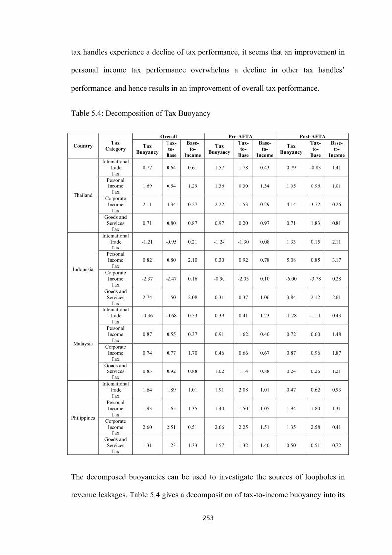
tax handles experience a decline of tax performance, it seems that an improvement in
personal income tax performance overwhelms a decline in other tax handles’
performance, and hence results in an improvement of overall tax performance.
Table 5.4: Decomposition of Tax Buoyancy
Country Tax Category
Overall Pre-AFTA Post-AFTA
Tax Buoyancy
Tax-to-
Base
Base-to-
Income
Tax Buoyancy
Tax-to-
Base
Base-to-
Income
Tax Buoyancy
Tax-to-
Base
Base-to-
Income
Thailand
International Trade Tax
0.77 0.64 0.61 1.57 1.78 0.43 0.79 -0.83 1.41
Personal Income
Tax 1.69 0.54 1.29 1.36 0.30 1.34 1.05 0.96 1.01
Corporate Income
Tax 2.11 3.34 0.27 2.22 1.53 0.29 4.14 3.72 0.26
Goods and Services
Tax 0.71 0.80 0.87 0.97 0.20 0.97 0.71 1.83 0.81
Indonesia
International Trade Tax
-1.21 -0.95 0.21 -1.24 -1.30 0.08 1.33 0.15 2.11
Personal Income
Tax 0.82 0.80 2.10 0.30 0.92 0.78 5.08 0.85 3.17
Corporate Income
Tax -2.37 -2.47 0.16 -0.90 -2.05 0.10 -6.00 -3.78 0.28
Goods and Services
Tax 2.74 1.50 2.08 0.31 0.37 1.06 3.84 2.12 2.61
Malaysia
International Trade Tax
-0.36 -0.68 0.53 0.39 0.41 1.23 -1.28 -1.11 0.43
Personal Income
Tax 0.87 0.55 0.37 0.91 1.62 0.40 0.72 0.60 1.48
Corporate Income
Tax 0.74 0.77 1.70 0.46 0.66 0.67 0.87 0.96 1.87
Goods and Services
Tax 0.83 0.92 0.88 1.02 1.14 0.88 0.24 0.26 1.21
Philippines
International Trade Tax
1.64 1.89 1.01 1.91 2.08 1.01 0.47 0.62 0.93
Personal Income
Tax 1.93 1.65 1.35 1.40 1.50 1.05 1.94 1.80 1.31
Corporate Income
Tax 2.60 2.51 0.51 2.66 2.25 1.51 1.35 2.58 0.41
Goods and Services
Tax 1.31 1.23 1.33 1.57 1.32 1.40 0.50 0.51 0.72
The decomposed buoyancies can be used to investigate the sources of loopholes in
revenue leakages. Table 5.4 gives a decomposition of tax-to-income buoyancy into its
253

constituent parts (i.e., tax-to-base and base-to-income). It is evident that the buoyancy
of the Thailand tax system is mainly due to the high tax-to-base buoyancy of
corporate income tax, especially in the post-AFTA period. The higher-than-unity
value of tax-to-base index suggests that there is a large improvement in the
administration of collection of this tax. However, it is notable that base-to-income
estimates of corporate income tax are quite low, indicating that tax bases for corporate
income taxes are quite rigid in both pre- and post-AFTA periods. This indicates that
trade liberalization does not result in a large expansion of the bases of this tax handle,
that it does not play any role in increasing corporate profit, stimulating investment,
and setting up of new businesses.
On the other hand, the estimate of base-to-income for personal income tax is quite
high, implying that the personal income tax base responds favourably to changes in
income. Unfortunately, the growth in personal income tax revenue lags behind the
growth in its base. This partly results in the less responsiveness of total tax revenue to
changes in GDP than the level that it should be.
For the international trade tax, the low values of tax-to-base and base-to-income
buoyancies probably signify not only both tax evasion and inefficient tax
administration but also the impact of trade liberalization. In the pre-AFTA period, the
value of tax-to-base buoyancy of international trade tax is very high while the value of
base-to-income buoyancy is very low, implying that during this period Thailand
successfully raised revenue from this tax source because of the nature of this tax. It
was easy to collect and the rate was set at very high levels, and was not due to the
level of international trade. However, in the post-AFTA period, the value of tax-to-
base buoyancy turns out to be very negative while the value of base-to-income
buoyancy is very buoyant, implying that, in this period trade liberalization results in a
254
substantial increase in the volume of international trade but the effect of the reduction
in the tariff rate overwhelms the effect of an increase in international trade, and hence
results in the reduction in international trade tax revenue. This finding may be
explained by the following factors. First, the pre-liberalization period is characterized
by a narrow base of international trade tax. It is not until the 1990s that exports and,
especially, imports expand considerably with the growth of GDP. Second, there are
weaknesses in international trade tax administration since the tax system, information
management, skills of tax authorities are poor during this period. Third, the
inefficiency of tax system contributes to loopholes for tax evasion and corruption.
For the goods and services tax, which also has the value of tax-to-base and base-to-
income estimates lower than unity, the reported values probably signifies tax evasion
and inefficient tax administration in the period that the country imposed business tax.
The results show tax-to-base estimates of the goods and services tax substantially
improves in the liberalization period, which is the same period that the country
changes the collection from business tax to value added tax. However, the decline of
base-to-income buoyancy from 0.97 to 0.81 reflects a low growth of private
consumption, the proxy base of this tax. The contraction of the consumption tax base
with respect to GDP implies that the country must be cautious in proceeding tax
policy and any policy related since the consumption tax base is the widest base
compared with other bases. In fact, both theory and experience in practice suggest that
the country should improve the revenue collection from goods and services tax to
mitigate the loss in international trade tax revenue. The rigid consumption tax base
may further cause the problem in revenue substitution.
Overall, for Thailand, trade liberalization improves the base-to-income buoyancy of
only international trade tax (from 0.43 to 1.41), but deteriorates the base-to-income
255

buoyancy of the other three major taxes; personal income tax (from 1.34 to 1.01),
corporate income tax (from 0.29 to 0.26), and goods and services tax (from 0.97 to
0.81). This indicates that trade liberalization, by joining AFTA, impacts on total tax
bases and seems to worsen total tax revenue. It causes the expansion of the
international trade tax base, it lowers the responsiveness of both direct and indirect
domestic tax bases, especially for the goods and services tax base which is the widest
tax base of the country. However, tax-to-base indexes of almost all tax handles,
except that of international trade tax, increase in the liberalization period, which
suggests that the post-AFTA tax structure is generally more flexible. This reflects the
improvement of tax administration of the country. The values of tax-to-base indexes
of personal income tax, corporate income tax and goods and services tax in the post-
liberalization period, which are equal to and higher than unity, suggest revenue
leakage is no longer a major problem of these taxes. For income and profit taxes, it
can be attributed to the improvement in tax administration, tax investigation, and
accounting audit. For goods and services tax, it can be attributed to the relative
effectiveness of tax reforms in the goods and services tax, which it does not only
make the tax system simpler but also reduce avenues for evasion and corruption. The
major reform includes the introduction of VAT, which the new tax reduces the
exemptions and shifts the system away from multiple business tax rates to single VAT
rate. The improvement in the performance of tax collection relative to the expansion
of the tax base is an important issue deriving from the results since it implies that
there is a success in tax reform after trade liberalization. However, since the desired
goal of tax reform is to make both the whole tax structure and the individual tax
handles more buoyant, the more rigidity of tax bases after trade is liberalized are the
major concern for the government but it is beyond the control of the tax authorities.
256

Considering its three neighbouring countries, Indonesia, Malaysia, and Philippines, it
is found that the reasons that make each country’s tax system rigid or flexible are
different. First, considering Indonesia, the rigidity of Indonesia’s tax system is mainly
due to the reduction in its corporate income tax collection. The negative sign of tax-
to-base coefficients means that, as the industry sector grows, Indonesia collects less
revenue from this tax. This is because Indonesia has continually cut its corporate
income tax rate in order to spur its investment and growth, especially after the
monetary crisis in 1997 which the country has experienced significant economic
instability. However, it seems that the loss of corporate income tax revenue is more
than covered by an increase of two tax sources, personal income and goods and
services taxes. For personal income tax, the success of revenue mobilization is mainly
due to the high buoyancy of base-to-income, especially in the post-AFTA period.
Base-to-income buoyancy of personal income tax substantially increases from only
0.78 to 3.17, implying that as Indonesia’s economy grows, more and more taxable
persons are included in the tax bracket as a result of substantial increase in wage and
salary level. For goods and services tax, both tax-to-base and base-to-income
buoyancies considerably increase in the post-AFTA period. This suggests that both
tax administration and tax base of goods and services tax have been largely improved
after the country entered into AFTA. The international trade tax has also experienced
an increase of both tax-to-base and base-to-income during the post-AFTA period,
implying that there is an improvement in the performance of tax authorities and
improvement in the level of imports and exports. This is a good sign for the country’s
tax reform since, in the liberalization period, there is no significant decrease in
international trade tax because both the tax base and tax authorities seem to have
257

improved. Furthermore, the tax base and the ability to collect the goods and services
tax, which is the broadest-based tax, have also been improved.
For Malaysia, it is found that corporate income tax is the only tax source that has
experienced an increase in tax buoyancy during the post-AFTA period. An
improvement of buoyancy of corporate income tax results from an increase in both
tax-to-base and base-to-income, especially the latter. The decline in tax buoyancy of
the international trade tax is rooted from the decrease in both tax-to-base and base-to-
income buoyancies, which indicates that not only AFTA may cause a reduction in
international trade tax collection via the reduction and elimination of a tariff, but
ASEAN Free Trade Agreement may also not have any impact in increasing the level
of international trade. On the other hand, the decline in tax buoyancy of personal
income and goods and services taxes comes only from the decrease in tax-to-base
buoyancy, suggesting that tax reform in the post-AFTA period may not be successful
in Malaysia since tax authorities do not show any sign of improvement regarding to
an expansion of tax bases.
Last, for Philippines, it is found that personal income tax is the only tax source that
has experienced an increase in tax buoyancy during the post-AFTA period, resulting
from an improvement in both tax-to-base and base-to-income. Corporate income tax
has experienced a little increase in tax-to-base buoyancy but a substantial decline in
base-to-income buoyancy, and hence results in the decline in corporate income tax
buoyancy during the liberalization period. This indicates that there is a contraction of
the corporate income tax base during the liberalization period. On the other hand, the
international trade tax and the goods and services tax have experienced a decline in
both tax-to-base and base-to-income buoyancies during the post-AFTA period.
Although the reduction of international trade tax revenue is an acceptable outcome of
258

AFTA, the decline of the level of trade is not an expected consequence. In addition,
the decline in tax-to-base and base-to-income buoyancies of goods and services tax
also indicates the failure of tax reform during the post-AFTA period.
5.6. Conclusion
Thailand and three neighbouring countries, including Indonesia, Malaysia, and
Philippines, have developed regional cooperation among Southeast Asian countries by
founding ASEAN which aims to accelerate economic growth, economic stability, and
other social progress among its members. In order to reach the aim of regional
economic development, ASEAN members have established the ASEAN FREE Trade
Area (AFTA) in 1992, which is an agreement concerning the elimination of trade
impediments. Since then, these member countries have liberalized its trade system
and have made significant progress towards a more open trade regime through the
reduction and elimination of both tariff and non-tariff barriers and through the
simplification of the tax system by conducting domestic tax reform. In principle, trade
liberalization may potentially have an impact on tax revenues both on tax productivity
and tax bases. Generally, trade liberalization is accompanied with tax reform and one
of the major objectives of tax reform is to increase tax productivity. Thus, in general,
trade liberalization should be associated with an increase in the country’s tax
productivity. Trade liberalization may also have an impact on the country’s tax bases
in many different ways. For example, trade liberalization usually results in an increase
in the country’s international trade volume, which is the tax base for international
trade tax. But trade liberalization itself is related to the reduction and elimination of
trade barriers, including tariffs, which directly reduces international trade tax revenue.
This leads to an ambiguity in the changes in trade tax revenue after liberalization. In
addition, other domestic tax bases may be affected by open trade regime. For instance,
259

trade liberalization, which is associated with an increase in the volume of trade, may
lead to a rise in corporate profit of exporting and importing companies which is an
important base for corporate income tax. It may also link with an expansion in the
consumption tax base since, in principle, trade liberalization may not only be related
to an increase in international trade, but it may also be related to an increase in
domestic trade by an increase in import volume. Trade liberalization may also have a
role in stimulating employment, especially for businesses in the international trade
sector, and hence drive up wages and salaries and consequently improve the personal
income tax base. Thus, in this chapter, we have investigated the impact of trade
liberalization, specifically AFTA, on revenue mobilization and tax productivity of
Thailand compared to those of three other ASEAN nations over the period 1972 to
2006 by applying the concept of tax buoyancy and tax elasticity.
Our results reveal that the tax system of Thailand and Philippines as a whole are
buoyant and elastic, while the tax system of Indonesia and Malaysia are not. The
buoyancy of Thailand’s and the Philippines tax system is mainly due to the high
buoyancy of corporate income taxes. By contrast, the rigidity of Indonesia tax system
is primarily caused by the inflexibility of the corporate income tax, while the rigidity
of Malaysia’s tax system is rooted in the inflexibility of all tax handles. Tax buoyancy
of pre- and post-AFTA indicates that Thailand and Malaysia have experienced a
decline in tax performance, whereas Indonesia and Philippines have experienced an
increase in tax performance during the liberalization period. The results are in line
with the analysis of tax elasticity which suggests that revenue mobilization of
Thailand and Malaysia is worse, while revenue mobilization of Indonesia and
Philippines has improved as a result of ASEAN Free Trade Area.
260

Considering the decomposed buoyancies, it appears that the high buoyancy of
Thailand’s tax system is particularly due to the high tax-to-base buoyancy of
corporate income tax, especially in the post-AFTA period. However, Thailand has
experienced a decline in base-to-income buoyancy during the post-AFTA period. An
increase in tax-to-base buoyancy can be inferred that the performance of corporate
income tax collection has been substantially improved. This is because recently both
countries have concentrated more on large companies that have a high potential in
paying large amount of tax, i.e. by setting up a large tax office which primarily
focuses on auditing these large businesses. However, a decline in base-to-income
buoyancy can be inferred that trade liberalization may be harmful to the ability to
make a profit of domestic companies. The results show that the Philippines seems to
follow the similar pattern that the high overall tax buoyancy resulted from an increase
in tax-to-base buoyancy of corporate income tax, though its base-to-income buoyancy
is very rigid in the liberalization period.
For Thailand, the other tax handle that is buoyant over the whole period of the study
is personal income tax, although the personal income tax buoyancy faces a small
decline during the post-AFTA period. The comparison of the decomposed buoyancies
of taxes to their respective bases and the bases to income indicates that an increase in
buoyancy of personal income tax is a contribution of an improvement in tax
administration and tax collection rather than an expansion of its base in the post-
liberalization period. This is because in the past decade, there is a large improvement
in the technology system that helps both tax authorities to calculate easily individual
income tax withholding and employers to withhold the correct amount from their
employees. This technology advance is particularly helpful since it correctly
withholds tax at source, and hence substantially reduces tax evasion. The other
261

country used in our study which shows an increase in the performance of personal
income tax collection is Philippines. However, the big difference between Thailand
and Philippines is that, for Philippines, there is no signal of personal income tax base
erosion during the post-AFTA period since there is an increase in both tax-to-base and
base-to-income personal income tax buoyancies after Philippines’s trade is
liberalized.
Two other individual tax handles which are not buoyant over the whole period of
study are the international trade tax and the goods and services tax. For the
international trade tax, the rigidity of this tax handle is mainly due to a substantial
decline in tax buoyancy in the liberalization period. The decline in tax buoyancy in
the post-AFTA period is as result of a large decline in tax-to-base buoyancy, not from
base-to-income buoyancy since the results show that there is a large increase in the
international trade tax base during this period. This suggests that the effect of tariff
reduction and the reduction in other related trade tax rates overwhelms an increase in
trade volume, and hence results in the reduction of international trade tax revenue.
The other two countries which have experienced a decline in the international trade
tax buoyancy are Malaysia and Philippines. Unlike Thailand, these two countries have
experienced a decrease in both tax-to-base and base-to-income, suggesting that these
countries may encounter a fall in trade volume as a result of trade liberalization.
Indonesia seems to be the only country which has experienced an increase in
international trade tax buoyancy. An increase in buoyancy of this tax handle results
from an increase in both tax-to-base and base-to-income, suggesting that trade
liberalization for Indonesia does not only have a positive impact on its trade volume,
but also has advantage on revenue productivity of this tax handle.
262

The rigidity of the goods and services tax is mainly due to a low tax-to-base buoyancy
in the pre-AFTA period and low base-to-income in the post-AFTA period. Although
tax buoyancy of the goods and services tax is quite rigid over the whole period, the
results show that this tax handle has a significant improvement in tax administration
and tax collection as its tax-to-base index substantially increases in the post-
liberalization period. This is mainly due to the VAT introduction in the context of
domestic tax reform as a result of liberalization. The introduction of VAT as a
replacement for the business tax makes the tax system simpler and reduces avenues
for evasion and corruption since it reduces the exemptions and shifts the system away
from multiple business tax rates to a single VAT rate. However, it is worth noting that
for the goods and services tax with base-to-income buoyancy lower than unity and
decreasing considerably from the pre-AFTA period, this indicates a low growth of
private consumption and tax authorities have very few options for improving
coefficients since the growth of this tax base is a macroeconomic problem outside the
control of tax authority. The government must be very careful in proceeding with its
macroeconomic policy because the contraction of the goods and services tax base
might cause the problem of revenue mobilization in the future. In addition, for
Thailand, the results suggest that the revenue mitigation policy by replacing tax
sources from international trade tax to broad-base goods and services tax is not very
successful. There are two other countries that seem to be faced with a similar
problem, Malaysia and Philippines. Indonesia seems to be the only country which is
successful in domestic tax reform since it does not have a negative impact on in
international trade tax revenue, but it also receives more revenue from goods and
services tax since both the tax base and tax administration of this tax handle are
improved in the post-AFTA period.
263
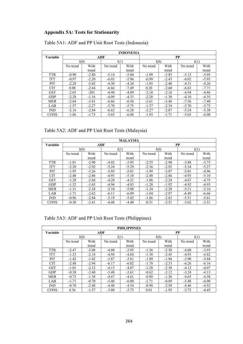
Appendix 5A: Tests for Stationarity
Table 5A1: ADF and PP Unit Root Tests (Indonesia)
INDONESIA Variable ADF PP
I(0) I(1) I(0) I(1) No trend With
trend No trend With
trend No trend With
trend No trend With
trend TTR -0.90 -2.80 -5.14 -5.04 -1.09 -2.83 -5.12 -5.05 ITT -0.97 -2.20 -6.03 -5.96 -0.99 -2.43 -6.02 -5.95 PIT -2.29 -3.02 -4.30 -4.24 -1.85 -2.40 -4.31 -4.26 CIT 0.08 -2.64 -6.66 -7.49 0.20 -2.60 -6.63 -7.71 GST -2.03 -201 -4.98 -4.89 -2.18 -2.16 -4.94 -4.86 GDP -2.28 -1.16 -4.09 -4.33 -2.28 -1.30 -4.10 -4.35 MER -2.64 -3.41 -6.66 -6.56 -2.61 -3.46 -7.56 -7.40 LAB -1.57 -2.27 -5.70 -5.75 -1.57 -2.34 -5.70 -5.75 IND -2.16 -2.84 -6.62 -6.28 -2.27 -2.87 -5.24 -5.38
CONS -1.86 -1.73 -5.65 -6.08 -1.93 -1.71 -5.65 -6.08
Table 5A2: ADF and PP Unit Root Tests (Malaysia)
MALAYSIA Variable ADF PP
I(0) I(1) I(0) I(1) No trend With
trend No trend With
trend No trend With
trend No trend With
trend TTR -1.81 -2.90 -4.02 -3.95 -2.55 -2.90 -3.88 -3.75 ITT -2.20 -2.92 -5.24 -5.29 -2.36 -2.92 -5.24 -5.27 PIT -1.95 -3.26 -5.05 -5.01 -1.99 -3.07 -5.01 -4.96 CIT -2.48 -2.86 -4.93 -5.10 -2.48 -2.86 -4.93 -5.10 GST -1.28 -2.68 -4.28 -4.21 -1.86 -2.24 -4.67 -4.75 GDP -1.32 -1.65 -4.94 -4.93 -1.28 -1.92 -4.92 -4.93 MER -1.31 -2.34 -5.10 -5.08 -1.34 -2.20 -5.21 -5.16 LAB -1.71 -2.62 -6.11 -6.09 -1.84 -2.87 -6.49 -6.66 IND -0.96 -2.84 -5.19 -5.02 -1.86 -2.82 -5.51 -5.61
CONS -0.30 -2.41 -4.48 -4.40 -0.51 -2.51 -3.62 -3.51
Table 5A3: ADF and PP Unit Root Tests (Philippines)
PHILIPPINES Variable ADF PP
I(0) I(1) I(0) I(1) No trend With
trend No trend With
trend No trend With
trend No trend With
trend TTR -2.47 -3.08 -4.08 -3.95 -1.56 -2.50 -4.08 -3.95 ITT -1.23 -2.18 -4.94 -4.84 -1.30 -2.45 -4.93 -4.82 PIT -1.42 -1.42 -3.87 -3.81 -1.89 -1.94 -3.90 -3.84 CIT -2.48 -2.94 -6.17 -6.02 -1.78 -2.33 -6.26 -6.16 GST -1.01 -2.12 -4.13 -4.07 -1.28 -2.38 -4.12 -4.07 GDP -0.38 -2.40 -3.48 -3.61 -0.62 -2.12 -3.24 -4.13 MER -0.73 -1.38 -4.67 -4.61 -0.80 -1.56 -4.65 -4.58 LAB -1.71 -0.70 -5.46 -6.00 -1.71 -0.69 -5.48 -6.00 IND -0.70 -2.48 -4.48 -4.54 -0.98 -2.50 -4.46 -4.52
CONS 0.36 -1.57 -3.80 -3.75 0.01 -1.93 -3.73 -4.45
264

Appendix 5B: Regression Results – Tax Buoyancy and Tax Elasticity
Tables below present the full regression results of tax buoyancy and tax elasticity
computed by the authors using Eviews econometric software. Overall tax system
(TTR) composes of four major taxes including international trade tax (ITT), personal
income tax (PIT), corporate income tax (CIT), and goods and services tax (GST).
Figures in parentheses [ ] below coefficient estimates are t values. R2 represents the
coefficient of determination. SER is the standard error of the regression. DW
represents the Durbin-Watson statistic, used to test the autocorrelation in the
residuals. JBNORM is the Jarque-Bera statistic for testing normality. The null
hypothesis is that errors are normally distributed. Serial LM is the Breusch-Godfrey
Lagrange multiplier test for serial correlation. The null hypothesis of the test is that
there is no serial correlation in the residuals. ARCH is a Lagrange multiplier (LM)
test for autoregressive conditional heteroscedasticity. The null hypothesis is that there
is no heteroscedasticity. RESET is Regression Specification Error Test, proposed by
Ramsey (1969) for testing functional form misspecification. The null hypothesis is
that there is no misspecification.
Tax Buoyancy; Combined Period (1972-2006)
Table 5B1: Thailand Tax Buoyancy of Major Taxes and the Tax System; 1972-2006
Constant Buoyancy R2 SER DW JBNORM Serial LM
ARCH RESET
ITT 2.09 [3.74]
0.77 [0.26]
0.92 0.20 1.72 1.95 F(1,30); 0.38
F(1,31); 0.01
F(1,30); 0.86
PIT -21.41 [-6.75]
1.69 [13.31]
0.98 0.17 2.24 0.49 F(1,30); 0.36
F(1,31); 0.08
F(1,30); 0.46
CIT -31.55 [-12.05]
2.11 [19.96]
0.99 0.15 1.91 0.30 F(1,30); 0.11
F(1,30); 0.13
F(1,28); 0.69
GST 5.10 [2.14]
0.71 [7.32]
0.92 0.14 2.17 0.56 F(1,30); 0.25
F(1,31); 0.07
F(1,30); 0.19
TTR -12.95 [-4.48]
1.44 [12.47]
0.98 0.14 2.23 0.03 F(1,30); 0.46
F(1,31); 0.04
F(1,30); 0.16
265

Table 5B2: Indonesia Tax Buoyancy of Major Taxes and the Tax System; 1972-2006
Constant Buoyancy R2 SER DW JBNORM Serial LM
ARCH RESET
ITT 52.43 [6.09]
-1.21 [-3.56]
0.91 0.27 2.03 0.23 F(2,27); 1.36
F(1,30); 1.04
F(1,28); 1.62
PIT 12.35 [2.73]
0.82 [2.41]
0.73 0.40 2.12 0.88 F(2,27); 2.26
F(1,30); 0.39
F(1,28); 0.78
CIT 84.11 [4.83]
-2.37 [-3.48]
0.89 0.41 2.26 1.02 F(2,29); 0.38
F(1,31); 0.08
F(1,30); 1.30
GST -50.66 [-2.55]
2.74 [2.24]
0.64 0.23 2.05 F(2,29); 2.21
F(1,31); 0.02
F(1,30); 0.62
TTR 10.84 [2.18]
0.86 [4.40]
0.91 0.20 1.92 2.74 F(2,29); 0.31
F(1,31); 0.02
F(2,29); 0.11
Table 5B3: Malaysia Tax Buoyancy of Major Taxes and the Tax System; 1972-2006
Constant Buoyancy R2 SER DW JBNORM Serial LM
ARCH RESET
ITT 30.42 [5.39]
-0.36 [-2.85]
0.74 0.20 1.69 1.32 F(2,29); 0.49
F(1,31); 0.13
F(1,30); 1.11
PIT -3.88 [-13.96]
0.87 [7.76]
0.95 0.14 1.88 2.10 F(2,29); 0.22
F(1,31); 1.16
F(2,29); 0.22
CIT 4.14 [2.24]
0.74 [3.79]
0.94 0.16 2.01 0.50 F(2,29); 0.17
F(1,31); 2.02
F(2,29); 0.36
GST 1.47 [3.53]
0.83 [8.46]
0.96 0.12 1.94 0.87 F(2,27); 0.64
F(1,30); 0.43
F(1,28); 0.32
TTR 8.44 [2.72]
0.60 [4.78]
0.93 0.12 2.03 0.52 F(2,27); 0.04
F(1,30); 1.21
F(2,27); 0.42
Table 5B4: Philippines Tax Buoyancy of Major Taxes and the Tax System; 1972-2006
Constant Buoyancy R2 SER DW JBNORM Serial LM
ARCH RESET
ITT -20.93 [-3.21]
1.64 [3.34]
0.84 0.24 2.03 0.84 F(2,29); 0.25
F(1,31); 0.30
F(1,30); 0.44
PIT -27.28 [-2.80]
1.93 [3.21]
0.96 0.19 2.06 0.93 F(2,27); 0.19
F(1,30); 0.01
F(1,28); 0.63
CIT -43.71 [-5.98]
2.60 [8.89]
0.93 0.23 2.07 0.71 F(2,27); 0.71
F(1,30); 0.96
F(1,28); 0.23
GST -10.91 [-2.43]
1.31 [0.38]
0.93 0.16 1.88 0.52 F(2,27); 0.34
F(1,30); 0.15
F(1,28); 0.79
TTR 14.11 [6.02]
1.76 [2.73]
0.95 0.16 1.95 1.10 F(2,27); 1.22
F(1,30); 0.12
F(1,28); 2.68
266

Tax Elasticity
Table 5B5: Thailand Tax Elasticity of Major Taxes and the Tax System; 1972-2006
Constant
Elasticity
Dummy
Slope dumm
y
R2 SER
DW
JBNORM
Serial LM
ARCH RESET
ITT -11.83 [-2.49]
1.34 [3.41]
25.00 [3.41]
-1.00 [-3.07]
0.93
0.20
1.65
1.22 F(2,27);
1.07
F(1,31);
0.15
F(1,28);
0.33 PIT -34.17
[-10.28] 2.21
[16.32] 29.20 [2.55]
-1.16 [-2.57]
0.98
0.16
2.07
0.40 F(2,27);
0.82
F(1,31);
7.49
F(1,28);
1.24 CIT -26.17
[-3.01] 1.89
[5.37] -18.32 [-2.85]
0.72 [2.87]
0.99
0.16
1.82
0.26 F(2,27);
0.32
F(1,31);
0.25
F(1,28);
0.64 GST
-16.62 [-6.22]
0.94 [8.63]
11.72 [2.33]
-0.47 [-2.65]
0.93
0.14
2.03
0.44 F(2,27);
0.17
F(1,31);
0.19
F(1,28);
0.31 TTR
-20.17 [-5.15]
1.73 [11.01]
12.72 [2.24]
-0.51 [-2.10]
0.98
0.14
2.08
1.36 F(2,27);
0.26
F(1,31);
0.04
F(1,28);
0.67
Table 5B6: Indonesia Tax Elasticity of Major Taxes and the Tax System; 1972-2006
Constant
Elasticity
Dummy
Slope dumm
y
R2 SER
DW
JBNORM
Serial LM
ARCH RESET
ITT 65.96 [3.05]
-1.74 [-2.02]
-20.85 [-4.81]
0.82 [2.05]
0.91
0.28
1.64
0.21 F(2,27);
2.11
F(1,31);
0.32
F(1,28);
1.57 PIT 18.54
[3.59] 0.12
[2.01] -66.84 [-2.19]
2.62 [2.40]
0.71
0.42
1.64
0.89 F(2,27);
1.20
F(1,31);
0.02
F(1,28);
1.98 CIT 46.37
[4.45] -0.87
[-2.09] 91.97 [2.35]
-3.60 [-2.36]
0.89
0.41
2.23
1.13 F(2,27);
0.51
F(1,31);
0.02
F(1,28);
2.77 GST
-34.47 [-2.58]
2.04 [3.23]
-25.13 [-2.43]
0.98 [2.05]
0.64
0.23
2.00
1.90 F(2,27);
1.79
F(1,31);
0.01
F(1,28);
0.83 TTR
6.98 [3.37]
0.65 [2.04]
1.45 [2.18]
0.57 [2.96]
0.91
0.21
1.99
3.28 F(2,27);
0.58
F(1,31);
0.05
F(2,27);
0.46
267

Table 5B7: Malaysia Tax Elasticity of Major Taxes and the Tax System; 1972-2006
Constant
Elasticity
Dummy
Slope dumm
y
R2 SER
DW
JBNORM
Serial LM
ARCH RESET
ITT 13.82 [2.36]
0.33 [3.79]
29.73 [2.25]
-1.21 [-2.16]
0.76
0.20
2.00
0.79 F(2,25);
0.28
F(1,30);
0.01
F(1,26);
0.63 PIT -1.33
[-2.53] 0.91
[4.23] 4.02
[4.65] -0.16
[-4.58] 0.95
0.15
1.85
1.82 F(2,27);
0.22
F(1,31);
1.14
F(2,27);
0.21 CIT 7.98
[2.64] 0.58
[3.81] -2.82
[-2.69] 0.12
[3.89] 0.94
0.16
2.03
0.42 F(2,27);
0.43
F(1,31);
2.06
F(1,28);
0.06 GST
-4.61 [-3.53]
1.08 [8.53]
18.65 [3.50]
-0.75 [-3.49]
0.96
0.11
2.05
0.53 F(2,25);
0.26
F(1,30);
4.01
F(1,26);
1.01 TTR
2.44 [4.01]
0.85 [3.40]
14.20 [2.10]
-0.57 [-2.93]
0.94
0.12
2.03
2.90 F(2,25);
0.07
F(1,30);
0.76
F(1,26);
0.06
Table 5B8: Philippines Tax Elasticity of Major Taxes and the Tax System; 1972-2006
Constant
Elasticity
Dummy
Slope dumm
y
R2 SER
DW
JBNORM
Serial LM
ARCH RESET
ITT -32.85 [-3.03]
2.18 [2.12]
44.89 [2.52]
-1.81 [-5.75]
0.84
0.24
2.10
0.42 F(2,27);
0.23
F(1,31);
1.90
F(1,28);
0.46 PIT 10.46
[2.56] 0.39
[6.33] -52.67 [-3.10]
2.13 [2.38]
0.96
0.19
2.14
0.65 F(2,25);
1.01
F(1,30);
0.01
F(1,26);
1.31 CIT -43.01
[-5.27] 2.86
[8.58] 30.58 [2.62]
-1.21 [-2.56]
0.95
0.20
2.07
0.01 F(2,25);
0.83
F(1,30);
001
F(1,26);
1.72 GST
-18.67 [-4.68]
1.62 [5.46]
18.57 [4.68]
-0.74 [-4.62]
0.94
0.16
1.93
0.30 F(2,25);
0.06
F(1,30);
0.54
F(1,26);
0.09 TTR
12.14 [2.71]
1.41 [3.62]
-25.20 [-2.76]
1.03 [2.71]
0.96
0.16
1.95
0.55 F(2,25);
0.87
F(1,30);
0.43
F(1,26);
1.60
Buoyancy; Pre-AFTA (1972-1991)
Table 5B9: Thailand Tax Buoyancy of Major Taxes and the Tax System; 1972-1991
Constant Buoyancy R2 SER DW JBNORM Serial LM
ARCH RESET
ITT -17.60 [-6.00]
1.57 [13.22]
0.95 0.15 1.99 1.84 F(2,24); 0.35
F(1,16); 0.01
F(1,15); 0.60
PIT -12.42 [-2.61]
1.36 [4.43]
0.99 0.10 2.00 0.34 F(2,14); 0.52
F(1,16); 1.35
F(1,15); 0.34
CIT -34.18 [-8.30]
2.22 [13.18]
0.98 0.12 1.60 0.81 F(2,12); 0.54
F(1,15); 1.57
F(1,13); 1.53
GST -1.45 [-2.42]
0.97 [23.42]
0.97 0.07 1.92 1.35 F(2,14); 0.05
F(1,16); 1.56
F(1,15); 0.42
TTR -22.67 [-10.63]
1.83 [21.38]
0.98 0.10 2.21 1.28 F(2,14); 0.73
F(1,16); 1.73
F(1,15); 0.37
268
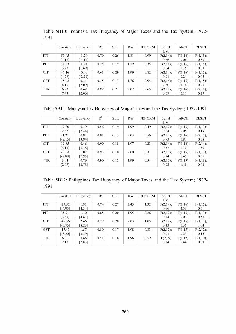
Table 5B10: Indonesia Tax Buoyancy of Major Taxes and the Tax System; 1972-1991
Constant Buoyancy R2 SER DW JBNORM Serial LM
ARCH RESET
ITT 53.45 [7.18]
-1.24 [-4.14]
0.79 0.26 1.81 0.99 F(2,14); 0.26
F(1,16); 0.06
F(1,15); 0.30
PIT 14.23 [3.27]
0.30 [1.69]
0.25 0.19 1.79 0.35 F(2,14); 0.04
F(1,16); 0.15
F(1,15); 0.03
CIT 47.16 [4.79]
-0.90 [-2.29]
0.61 0.29 1.99 0.82 F(2,14); 0.01
F(1,16); 0.24
F(1,15); 0.05
GST 15.42 [4.10]
0.31 [2.09]
0.35 0.17 1.76 0.94 F(2,14); 2.80
F(1,16); 3.14
F(1,15); 0.23
TTR 6.22 [7.43]
0.68 [2.06]
0.88 0.22 2.07 3.65 F(2,14); 0.09
F(1,16); 0.11
F(2,14); 0.29
Table 5B11: Malaysia Tax Buoyancy of Major Taxes and the Tax System; 1972-1991
Constant Buoyancy R2 SER DW JBNORM Serial LM
ARCH RESET
ITT 12.30 [2.37]
0.39 [2.44]
0.56 0.19 1.99 0.49 F(2,12); 0.04
F(1,15); 0.05
F(1,13); 0.19
PIT -1.21 [-2.15]
0.91 [3.94]
0.91 0.13 2.03 0.56 F(2,14); 0.73
F(1,16); 0.81
F(2,14); 0.38
CIT 10.85 [3.13]
0.46 [8.38]
0.90 0.18 1.97 0.23 F(2,14); 0.32
F(1,16); 1.10
F(2,14); 1.30
GST -3.19 [-2.88]
1.02 [7.95]
0.93 0.10 2.00 0.31 F(2,12); 0.94
F(1,15); 1.45
F(1,13); 0.35
TTR 3.94 [2.07]
0.79 [2.78]
0.90 0.12 1.99 0.54 F(2,12); 0.05
F(1,15); 1.48
F(1,13); 0.02
Table 5B12: Philippines Tax Buoyancy of Major Taxes and the Tax System; 1972-1991
Constant Buoyancy R2 SER DW JBNORM Serial LM
ARCH RESET
ITT -25.52 [-4.95]
1.91 [4.34]
0.74 0.27 2.43 1.32 F(2,14); 0.66
F(1,16); 2.53
F(1,15); 0.51
PIT 38.71 [3.33]
1.40 [4.87]
0.85 0.20 1.95 0.26 F(2,12); 0.14
F(1,15); 0.03
F(1,13); 0.55
CIT -45.56 [-5.75]
2.66 [8.23]
0.79 0.20 2.03 1.05 F(2,12); 0.43
F(1,15); 0.36
F(1,13); 1.04
GST -17.43 [-3.20]
1.57 [3.59]
0.89 0.17 1.98 0.83 F(2,12); 0.01
F(1,15); 0.23
F(2,12); 0.15
TTR 6.61 [2.17]
0.66 [2.83]
0.51 0.16 1.96 0.59 F(2,9); 0.84
F(1,12); 0.44
F(1,10); 0.68
269

Buoyancy; Post-AFTA (1992-2006)
Table 5B13: Thailand Tax Buoyancy of Major Taxes and the Tax System; 1992-2006
Constant Buoyancy R2 SER DW JBNORM Serial LM
ARCH RESET
ITT -50.80 [-2.41]
0.79 [4.99]
0.71 0.21 2.43 1.81 F(2,10); 0.93
F(1,12); 0.01
F(1,11); 3.01
PIT -4.98 [-2.71]
1.05 [3.03]
0.44 0.20 1.97 0.48 F(2,10); 0.06
F(1,12); 0.68
F(1,11); 0.15
CIT -83.89 [-2.78]
4.14 [3.56]
0.88 0.16 2.37 0.33 F(2,10); 1.53
F(1,12); 0.02
F(1,11); 1.11
GST 4.96 [2.40]
0.71 [8.47]
0.88 0.16 2.38 0.74 F(2,10); 2.59
F(1,12); 0.11
F(1,11); 0.71
TTR -21.42 [-2.91]
1.77 [2.15]
0.62 0.19 2.40 1.44 F(2,10); 0.34
F(1,12); 0.09
F(1,11); 0.95
Table 5B14: Indonesia Tax Buoyancy of Major Taxes and the Tax System; 1992-2006
Constant Buoyancy R2 SER DW JBNORM Serial LM
ARCH RESET
ITT 14.04 [2.37]
1.33 [2.19]
0.86 0.26 1.87 1.40 F(2,10); 2.72
F(1,12); 0.48
F(1,11); 0.83
PIT -10.95 [-3.22]
5.08 [2.07]
0.59 0.58 1.95 0.13 F(2,10); 0.04
F(1,12); 0.62
F(1,11); 0.14
CIT 177.91 [6.89]
-6.00 [-6.00]
0.79 0.53 2.03 1.00 F(2,10); 0.01
F(1,12); 0.01
F(1,11); 0.20
GST -77.85 [-3.70]
3.84 [4.87]
0.81 0.24 1.96 0.49 F(2,10); 0.67
F(1,12); 0.27
F(1,11); 2.92
TTR 13.34 [2.33]
1.44 [0.65]
0.49 0.20 1.81 0.89 F(2,10); 1.87
F(1,12); 0.02
F(1,11); 0.11
Table 5B15: Malaysia Tax Buoyancy of Major Taxes and the Tax System; 1992-2006
Constant Buoyancy R2 SER DW JBNORM Serial LM
ARCH RESET
ITT -64.28 [-2.10]
-1.28 [-4.64]
0.89 0.16 2.13 3.76 F(2,9); 0.55
F(1,12); 0.23
F(1,10); 2.42
PIT 3.48 [2.44]
0.72 [2.30]
0.61 0.17 1.64 3.36 F(2,10); 0.41
F(1,12); 0.89
F(1,11); 0.51
CIT 0.82 [2.30]
0.87 [3.94]
0.69 0.15 1.90 0.83 F(2,10); 0.04
F(1,12); 0.01
F(1,11); 0.07
GST 16.17 [4.03]
0.24 [4.13]
0.67 0.12 2.11 0.51 F(2,9); 0.81
F(1,12); 1.76
F(1,10); 1.93
TTR 17.90 [3.21]
0.42 [3.48]
0.68 0.12 2.25 1.55 F(2,9); 0.43
F(1,12); 0.13
F(1,10); 0.87
270

Table 5B16: Philippines Tax Buoyancy of Major Taxes and the Tax System; 1992-2006
Constant Buoyancy R2 SER DW JBNORM Serial LM
ARCH RESET
ITT 33.57 [2.05]
0.47 [3.02]
0.85 0.19 1.83 2.94 F(2,9); 1.28
F(1,12); 0.49
F(1,10); 2.34
PIT -6.11 [-2.57]
1.94 [4.71]
0.75 0.15 2.18 1.27 F(2,10); 0.23
F(1,12); 0.05
F(1,11); 0.50
CIT -12.27 [-2.24]
1.35 [3.23]
0.66 0.20 1.84 0.22 F(2,9); 0.01
F(1,12); 2.48
F(1,10); 0.07
GST 9.47 [2.88]
0.50 [2.16]
0.42 0.16 1.75 1.09 F(2,9); 0.85
F(1,12); 1.51
F(1,10); 0.89
TTR -34.93 [-2.50]
2.32 [4.06]
0.86 0.16 1.82 0.47 F(2,12); 0.58
F(1,15); 0.01
F(1,13); 0.85
271

Appendix 5C: Regression Results – The Decomposition of Tax Buoyancy
Tables below present the full regression results of the decomposition of tax buoyancy
computed by the authors using Eviews econometric software. The decomposition is
done for all four major taxes including international trade tax (ITT), personal income
tax (PIT), corporate income tax (CIT), and goods and services tax (GST).
Merchandise trade as a share of GDP is used as a proxy base for international trade
tax. Compensation of employees is used as a proxy base for personal income tax. The
share of industry in GDP is used as a proxy base for corporate income tax. Household
final consumption expenditure is used as a proxy base for consumption tax. Figures in
parentheses [ ] below coefficient estimates are t values. R2 represents the coefficient
of determination. SER is the standard error of the regression. DW represents the
Durbin-Watson statistic, used to test the autocorrelation in the residuals. JBNORM is
the Jarque-Bera statistic for testing normality. The null hypothesis is that errors are
normally distributed. Serial LM is the Breusch-Godfrey Lagrange multiplier test for
serial correlation. The null hypothesis of the test is that there is no serial correlation in
the residuals. ARCH is a Lagrange multiplier (LM) test for autoregressive conditional
heteroscedasticity. The null hypothesis is that there is no heteroscedasticity. RESET is
Regression Specification Error Test, proposed by Ramsey (1969) for testing
functional form misspecification. The null hypothesis is that there is no
misspecification.
272

The Decomposition of Tax Buoyancy; Combined Period (1972-2006)
Table 5C1: Thailand – Tax-to-Base; 1972-2006
Constant Tax-to-Base
R2 SER DW JBNORM Serial LM
ARCH RESET
ITT 18.84 [12.98]
0.64 [2.52]
0.92 0.21 1.59 0.52 F(2,29); 0.78
F(1,31); 0.12
F(1,30); 0.99
PIT 10.23 [2.58]
0.54 [2.06]
0.99 0.15 1.91 0.32 F(2,29); 0.03
F(1,31); 0.01
F(2,29); 0.81
CIT -5.11 [-2.79]
3.34 [6.63]
0.97 0.23 1.86 0.14 F(2,25); 1.47
F(1,29); 0.16
F(1,26); 2.72
GST -3.11 [-2.70]
0.80 [7.08]
0.92 0.14 2.20 0.53 F(2,29); 0.31
F(1,31); 0.14
F(1,30); 0.26
Table 5C2: Thailand – Base-to-Income; 1972-2006
Constant Base-to-Income
R2 SER DW JBNORM Serial LM
ARCH RESET
ITT -11.04 [-2.77]
0.61 [3.89]
0.96 0.08 1.81 0.66 F(2,29); 0.21
F(1,31); 1.02
F(1,30); 0.32
PIT 15.42 [3.87]
1.29 [8.06]
0.54 0.16 1.92 0.39 F(2,29); 0.04
F(1,31); 0.23
F(1,30); 0.07
CIT -3.29 [-16.16]
0.27 [34.03]
0.99 0.02 2.05 1.48 F(2,29); 0.22
F(1,31); 0.71
F(1,30); 0.49
GST 2.70 [5.41]
0.87 [44.64]
0.99 0.02 1.91 1.35 F(2,29); 2.18
F(1,31); 0.30
F(1,30); 0.52
Table 5C3: Indonesia – Tax-to-Base; 1972-2006
Constant Tax-to-Base
R2 SER DW JBNORM Serial LM
ARCH RESET
ITT 19.94 [13.01]
-0.95 [-25.54]
0.91 0.27 1.86 0.18 F(2,29); 0.58
F(1,31); 0.54
F(1,30); 0.68
PIT 6.02 [2.35]
0.80 [2.94]
0.73 0.39 1.90 0.71 F(2,29); 0.07
F(1,31); 0.23
F(1,30); 0.08
CIT 19.55 [2.27]
-2.47 [-2.49]
0.89 0.40 2.09 0.38 F(2,29); 0.51
F(1,31); 0.41
F(1,30); 0.98
GST -15.02 [-3.25]
1.50 [8.05]
0.95 0.23 1.75 021 F(2,29); 0.38
F(1,31); 0.01
F(1,30); 1.24
Table 5C4: Indonesia – Base-to-Income; 1972-2006
Constant Base-to-Income
R2 SER DW JBNORM Serial LM
ARCH RESET
ITT -1.42 [-2.76]
0.21 [3.01]
0.55 0.15 1.87 0.14 F(2,29); 0.30
F(1,31); 0.04
F(1,30); 0.34
PIT -35.44 [-2.65]
2.10 [3.40]
0.94 0.28 2.32 0.82 F(2,29); 1.87
F(1,31); 0.04
F(1,30); 0.56
CIT -3.74 [-4.03]
0.16 [4.44]
0.86 0.05 1.93 0.38 F(2,29); 0.04
F(1,31); 1.07
F(1,30); 0.41
GST -2.61 [-2.96]
2.08 [4.15]
0.99 0.06 1.78 0.23 F(2,29); 0.23
F(1,31); 0.13
F(1,30); 0.50
273

Table 5C5: Malaysia – Tax-to-Base; 1972-2006
Constant Tax-to-Base
R2 SER DW JBNORM Serial LM
ARCH RESET
ITT 17.99 [4.92]
-0.68 [-6.95]
0.74 0.20 2.05 0.72 F(2,27); 0.23
F(1,30); 0.60
F(1,28); 0.46
PIT 9.57 [3.65]
0.55 [4.37]
0.95 0.13 2.27 0.14 F(2,29); 0.49
F(1,31); 0.27
F(1,30); 0.32
CIT 19.85 [7.21]
0.77 [2.60]
0.94 0.16 1.96 0.16 F(2,29); 0.01
F(1,31); 0.43
F(1,30); 0.56
GST -11.29 [-4.22]
0.92 [8.24]
0.96 0.11 1.90 0.51 F(2,27); 0.79
F(1,30); 1.23
F(1,28); 0.41
Table 5C6: Malaysia – Base-to-Income; 1972-2006
Constant Base-to-Income
R2 SER DW JBNORM Serial LM
ARCH RESET
ITT -8.43 [-7.63]
0.53 [12.05]
0.97 0.07 1.81 0.32 F(2,27); 0.01
F(1,30); 0.49
F(2,27); 0.10
PIT 13.28 [8.45]
0.37 [5.63]
0.84 0.14 2.18 0.64 F(2,29); 0.31
F(1,31); 2.49
F(1,30); 0.47
CIT -4.36 [-5.36]
1.70 [5.15]
0.93 0.03 1.73 0.57 F(2,29); 0.14
F(1,31); 1.82
F(1,30); 0.57
GST 2.11 [3.90]
0.88 [4.04]
0.99 0.03 1.95 0.30 F(2,27); 0.22
F(1,30); 0.09
F(1,28); 0.91
Table 5C7: Philippines – Tax-to-Base; 1972-2006
Constant Tax-to-Base
R2 SER DW JBNORM Serial LM
ARCH RESET
ITT 24.00 [10.84]
1.89 [3.55]
0.84 0.25 2.00 0.55 F(2,27); 0.37
F(1,30); 0.36
F(1,28); 0.96
PIT 7.80 [2.55]
1.65 [5.76]
0.96 0.17 1.95 1.67 F(2,27); 0.18
F(1,30); 0.34
F(1,28); 0.63
CIT -30.71 [-7.79]
2.51 [2.21]
0.94 0.21 2.21 0.42 F(2,27); 1.48
F(1,30); 0.03
F(1.28); 0.38
GST -8.56 [-2.84]
1.23 [4.32]
0.93 0.16 1.98 0.67 F(2,27); 0.55
F(1,30); 0.10
F(1,28); 0.95
Table 5C8: Philippines – Base-to-Income; 1972-2006
Constant Base-to-Income
R2 SER DW JBNORM Serial LM
ARCH RESET
ITT -21.03 [-2.60]
1.01 [2.27]
0.96 0.09 1.98 1.61 F(2,27); 0.25
F(1,30); 0.36
F(2,27); 0.89
PIT -12.62 [-3.30]
1.35 [2.57]
0.96 0.16 1.99 0.12 F(2,27); 0.36
F(1,30); 0.22
F(1,28); 0.35
CIT -9.45 [-7.05]
0.51 [5.15]
0.95 0.02 1.94 0.49 F(2,27); 1.67
F(1,30); 0.03
F(1,28); 0.53
GST -1.87 [-2.73]
1.33 [2.19]
0.99 0.01 2.32 0.43 F(2,27); 2.02
F(1,30); 0.21
F(1,28); 0.55
274

The Decomposition of Tax Buoyancy; Pre-AFTA (1972-1991)
Table 5C9: Thailand – Tax-to-Base; 1972-1991
Constant Tax-to-Base
R2 SER DW JBNORM Serial LM
ARCH RESET
ITT 14.64 [10.41]
1.78 [6.09]
0.97 0.11 2.37 0.67 F(2,14); 1.40
F(1,16); 0.30
F(1,15); 1.50
PIT 3.39 [3.87]
0.30 [2.08]
0.99 0.11 1.99 0.41 F(2,12); 0.07
F(1,15); 0.74
F(1,13); 0.91
CIT 6.46 [2.45]
1.53 [8.74]
0.97 0.16 1.89 1.26 F(2,12); 0.04
F(1,15); 0.97
F(1,13); 14.52
GST -6.55 [-5.02]
0.20 [5.92]
0.97 0.07 1.92 0.31 F(2,14); 0.07
F(1,16); 1.84
F(1,15); 0.36
Table 5C10: Thailand – Base-to-Income; 1972-1991
Constant Base-to-Income
R2 SER DW JBNORM Serial LM
ARCH RESET
ITT -6.70 [-2.56]
0.43 [4.06]
0.84 0.08 1.83 0.68 F(2,12); 0.04
F(1,15); 0.27
F(1,13); 1.19
PIT 14.27 [2.93]
1.34 [6.92]
0.57 0.13 1.65 0.55 F(2,14); 0.31
F(1,16); 0.01
F(1,15); 0.57
CIT -3.69 [-9.28]
0.29 [18.10]
0.96 0.02 2.17 1.18 F(2,14); 0.23
F(1,16); 0.43
F(1,15); 0.94
GST 2.73 [6.20]
0.97 [17.23]
0.99 0.01 1.89 0.16 F(2,10); 1.44
F(1,12); 0.93
F(1,11); 1.62
Table 5C11: Indonesia – Tax-to-Base; 1972-1991
Constant Tax-to-Base
R2 SER DW JBNORM Serial LM
ARCH RESET
ITT 17.11 [7.88]
-1.30 [-2.15]
0.80 0.25 2.05 1.21 F(2,14); 0.11
F(1,16); 0.06
F(1,15); 0.84
PIT 41.64 [11.92]
0.92 [6.29]
0.85 0.29 1.88 0.45 F(2,14); 0.41
F(1,16); 1.70
F(1,15); 0.45
CIT 14.51 [3.67]
-2.05 [-2.52]
0.67 0.27 2.33 0.55 F(2,14); 0.92
F(1,16); 0.14
F(1,15); 1.52
GST -11.99 [-2.73]
0.37 [8.58]
0.92 0.22 1.94 1.45 F(2,14); 0.58
F(1,16); 1.55
F(1,15); 0.72
Table 5C12: Indonesia – Base-to-Income; 1972-1991
Constant Base-to-Income
R2 SER DW JBNORM Serial LM
ARCH RESET
ITT 1.53 [2.48]
0.08 [2.34]
0.33 0.09 1.76 0.47 F(2,10); 0.80
F(1,14); 0.49
F(1,11); 0.82
PIT 68.32 [18.04]
0.78 [11.66]
0.96 0.15 2.08 1.89 F(2,14); 0.42
F(1,16); 0.82
F(1,15); 2.35
CIT -3.09 [-2.23]
0.10 [2.16]
0.69 0.06 2.07 0.38 F(2,14); 0.25
F(1,16); 0.88
F(1,15); 0.32
GST -2.25 [-3.10]
1.06 [9.74]
0.97 0.08 1.81 0.44 F(2,14); 0.08
F(1,16); 0.01
F(1,15); 0.14
275

Table 5C13: Malaysia – Tax-to-Base; 1972-1991
Constant Tax-to-Base
R2 SER DW JBNORM Serial LM
ARCH RESET
ITT 17.50 [6.12]
0.41 [2.83]
0.70 0.17 1.52 1.81 F(2,14); 0.53
F(1,16); 0.23
F(1,15); 1.35
PIT -15.23 [-2.50]
1.62 [5.92]
0.91 0.13 1.83 0.34 F(2,14); 0.13
F(1,16); 0.01
F(1,15); 0.22
CIT 14.57 [3.61]
0.66 [3.38]
0.88 0.17 1.92 1.23 F(2,12); 1.17
F(1,15); 0.75
F(1,13); 0.32
GST -5.33 [-2.71]
1.14 [13.68]
0.95 0.09 1.93 0.73 F(2,12); 0.20
F(1,15); 0.06
F(2,12); 0.24
Table 5C14: Malaysia – Base-to-Income; 1972-1991
Constant Base-to-Income
R2 SER DW JBNORM Serial LM
ARCH RESET
ITT -25.67 [-3.91]
1.23 [4.77]
0.90 0.06 1.58 0.66 F(2,12); 0.46
F(1,15); 0.98
F(1,13); 2.21
PIT 12.55 [4.24]
0.40 [3.26]
0.93 0.07 1.95 0.74 F(2,14); 1.93
F(1,16); 0.04
F(2,14); 0.91
CIT 15.48 [2.09]
0.67 [2.78]
0.85 0.04 2.00 0.30 F(2,14); 0.40
F(1,16); 2.65
F(1,15); 0.43
GST 2.32 [2.38]
0.88 [21.60]
0.98 0.37 2.06 0.17 F(2,12); 0.32
F(1,15); 0.13
F(1,13); 0.01
Table 5C15: Philippines – Tax-to-Base; 1972-1991
Constant Tax-to-Base
R2 SER DW JBNORM Serial LM
ARCH RESET
ITT 13.48 [2.31]
2.08 [3.53]
0.80 0.26 1.90 0.55 F(2,12); 0.26
F(1,15); 0.33
F(1,13); 0.73
PIT 9.53 [3.01]
1.50 [4.38]
0.86 0.19 1.89 1.12 F(2,12); 0.02
F(1,15); 0.28
F(1,13); 1.11
CIT -31.83 [-4.26]
2.25 [2.19]
0.78 0.21 1.87 0.65 F(2,12); 0.01
F(1,15); 0.35
F(1,13); 0.32
GST -10.64 [-5.59]
1.32 [2.72]
0.89 0.17 2.08 1.05 F(2,12); 0.06
F(1,15); 0.12
F(1,13); 0.01
Table 5C16: Philippines – Base-to-Income; 1972-1991
Constant Base-to-Income
R2 SER DW JBNORM Serial LM
ARCH RESET
ITT -1.46 [-3.64]
1.01 [3.54]
0.55 0.08 1.75 0.50 F(2,12); 0.36
F(1,15); 0.86
F(1,13); 0.90
PIT -18.21 [-5.25]
1.05 [3.52]
0.96 0.17 1.88 1.27 F(2,12); 0.13
F(1,15); 0.11
F(1,13); 0.62
CIT -3.15 [-3.77]
1.51 [10.61]
0.91 0.02 1.85 0.67 F(2,12); 0.28
F(1,15); 0.45
F(1,13); 1.37
GST -1.61 [-8.18]
1.40 [2.60]
0.99 0.01 2.13 1.22 F(2,12); 1.26
F(1,15); 0.29
F(1,13); 0.32
276

The Decomposition of Tax Buoyancy; Post-AFTA (1992-2006)
Table 5C17: Thailand – Tax-to-Base; 1992-2006
Constant Tax-to-Base
R2 SER DW JBNORM Serial LM
ARCH RESET
ITT 25.50 [15.41]
-0.83 [-2.23]
0.72 0.21 2.18 2.66 F(2,9); 0.32
F(1,12); 1.01
F(1,10); 0.42
PIT 6.52 [2.03]
0.96 [6.77]
0.74 0.15 1.98 0.61 F(2,9); 2.05
F(1,12); 0.39
F(1,10); 1.42
CIT 8.45 [2.23]
3.72 [2.04]
0.81 0.21 2.05 0.58 F(2,9); 0.39
F(1,12); 0.33
F(1,10); 1.66
GST -3.01 [-15.46]
1.83 [2.30]
0.50 0.19 2.28 0.94 F(2,9); 1.15
F(1,12); 0.01
F(1,10); 1.86
Table 5C18: Thailand – Base-to-Income; 1992-2006
Constant Base-to-Income
R2 SER DW JBNORM Serial LM
ARCH RESET
ITT 20.61 [2.47]
1.41 [7.54]
0.93 0.07 2.29 0.28 F(2,10); 2.56
F(1,12); 0.69
F(1,11); 1.31
PIT 20.98 [3.25]
1.01 [2.28]
0.39 0.19 2.29 0.11 F(2,10); 2.01
F(1,12); 0.09
F(1,11); 1.80
CIT -2.85 [-2.58]
0.26 [5.97]
0.87 0.02 1.67 0.28 F(2,10); 0.44
F(1,12); 0.01
F(1,11); 0.28
GST 4.26 [12.54]
0.81 [5.81]
0.98 0.01 1.85 1.00 F(2,14); 4.06
F(1,16); 1.40
F(1,15); 0.16
Table 5C19: Indonesia – Tax-to-Base; 1992-2006
Constant Tax-to-Base
R2 SER DW JBNORM Serial LM
ARCH RESET
ITT 20.36 [14.89]
0.15 [4.17]
0.86 0.27 2.08 0.56 F(2,9); 0.87
F(1,12); 0.54
F(1,10); 0.56
PIT 3.83 [2.23]
0.85 [3.15]
0.65 0.54 1.71 1.45 F(2,10); 0.18
F(1,12); 0.50
F(1,11); 0.15
CIT 36.79 [3.27]
-3.78 [-4.17]
0.47 0.47 1.98 0.93 F(2,10); 0.05
F(1,12); 0.22
F(1,11); 0.03
GST -3.58 [-5.65]
2.12 [4.96]
0.65 0.27 1.56 1.98 F(2,10); 0.33
F(1,12); 0.01
F(1,11); 0.92
Table 5C20: Indonesia – Base-to-Income; 1992-2006
Constant Base-to-Income
R2 SER DW JBNORM Serial LM
ARCH RESET
ITT 58.98 [2.30]
2.11 [3.67]
0.46 0.18 2.06 0.38 F(2,9); 0.19
F(1,12); 0.34
F(1,10); 0.45
PIT -61.18 [-2.82]
3.17 [3.73]
0.77 0.36 2.24 0.11 F(2,10); 1.64
F(1,12); 0.61
F(1,11); 1.71
CIT -3.52 [-2.28]
0.28 [2.88]
0.73 0.03 1.86 0.27 F(2,9); 0.27
F(1,12); 0.71
F(1,10); 0.23
GST 9.66 [7.79]
2.61 [2.50]
0.99 0.02 1.84 0.30 F(2,10); 0.63
F(1,12); 0.25
F(1,11); 1.11
277

Table 5C21: Malaysia – Tax-to-Base; 1992-2006
Constant Tax-to-Base
R2 SER DW JBNORM Serial LM
ARCH RESET
ITT 26.98 [5.09]
-1.11 [-10.81]
0.83 0.19 1.90 0.14 F(2,9); 0.36
F(1,12); 0.05
F(1,10); 2.25
PIT 8.21 [2.39]
0.60 [3.89]
0.79 0.12 2.29 0.21 F(2,10); 1.12
F(1,12); 0.45
F(1,11); 3.19
CIT 34.30 [2.24]
0.96 [3.27]
0.72 0.15 2.02 0.05 F(2,9); 0.16
F(1,12); 0.01
F(1,10); 2.13
GST 16.06 [4.35]
0.26 [2.70]
0.68 0.12 2.15 0.40 F(2,9); 0.99
F(1,12); 2.39
F(1,10); 2.14
Table 5C22: Malaysia – Base-to-Income; 1992-2006
Constant Base-to-Income
R2 SER DW JBNORM Serial LM
ARCH RESET
ITT -5.76 [-3.24]
0.43 [6.14]
0.76 0.06 1.56 0.56 F(2,9); 0.58
F(1,12); 0.32
F(1,10); 0.37
PIT -13.19 [-2.09]
1.48 [3.19]
0.29 0.19 2.03 0.12 F(2,9); 0.44
F(1,12); 0.40
F(1,10); 1.05
CIT -5.24 [-4.46]
1.87 [3.45]
0.92 0.03 2.18 0.20 F(2,9); 0.89
F(1,12); 0.77
F(1,10); 0.50
GST -6.16 [-3.38]
1.21 [16.77]
0.99 0.02 1.91 0.88 F(2,9); 0.47
F(1,12); 0.06
F(1,10); 1.37
Table 5C23: Philippines – Tax-to-Base; 1992-2006
Constant Tax-to-Base
R2 SER DW JBNORM Serial LM
ARCH RESET
ITT 31.71 [9.09]
0.62 [8.45]
0.92 0.14 1.87 0.38 F(2,9); 0.38
F(1,12); 0.10
F(1,10); 2.72
PIT 12.56 [2.16]
1.80 [5.05]
0.75 0.16 1.86 1.10 F(2,9); 0.19
F(1,12); 0.09
F(1,10); 0.34
CIT -30.89 [-4.06]
2.58 [2.22]
0.58 0.22 1.80 0.57 F(2,9); 0.10
F(1,12); 0.01
F(1,10); 0.21
GST 9.32 [2.03]
0.51 [2.62]
0.42 0.16 1.77 1.27 F(2,9); 0.85
F(1,12); 1.40
F(1,10); 0.97
Table 5C24: Philippines – Base-to-Income; 1992-2006
Constant Base-to-Income
R2 SER DW JBNORM Serial LM
ARCH RESET
ITT 14.82 [2.05]
0.93 [2.90]
0.92 0.08 2.18 0.78 F(2,9); 4.01
F(1,12); 0.25
F(1,10); 1.30
PIT -30.13 [-6.14]
1.31 [6.70]
0.93 0.14 1.99 0.77 F(2,9); 0.12
F(1,12); 0.34
F(1,10); 0.26
CIT -3.69 [-3.66]
0.41 [10.27]
0.97 0.02 2.29 1.16 F(2,9); 0.84
F(1,12); 1.29
F(1,10); 1.54
GST -8.83 [-3.97]
0.72 [3.44]
0.99 0.01 2.35 0.33 F(2,9); 2.00
F(1,12); 1.32
F(1,10); 1.12
278
Appendix 5D: Cointegration Test – Tax Buoyancy and Tax Elasticity
Tables below present the cointegration test for variable used to calculate tax buoyancy
and tax elasticity computed by the authors using Eviews econometric software. In this
study, the Engle-Granger (EG) approach is applied to test for cointegration. The
concept of the EG approach is that if cointegration genuinely exists between
variables, the error term should remain roughly constant over time, i.e. it should be
stationary. However, if the error term is tending to increase over time, this implies
that the variables are not cointegrated. There are two steps in performing the EG
cointegration test. After it is found that all variables in all countries are I(1) in the
stationary test using ADF and PP approaches, the first step here is to run a standard
OLS regression on the variables. The residuals obtained from the first step will be
used to test for unit root by using the ADF and PP procedure. If a unit root does not
exist, the residuals are stationary and we can conclude that the variables under
investigation are cointegrated, and therefore buoyancy, elasticity, and decomposition
results are meaningful.
Figures in parentheses [ ] below coefficient estimates are t values. The residual tests
using both ADF and PP methods report a t-ratio which is used to test the null
hypothesis that the residual has a unit root.
Cointegration test for variables used for computing tax buoyancy; Combined
period (1972-2006)
For combined period (1972-2006), the critical values for both the ADF and the PP
tests are as follows; 90% critical value is -1.61, 95% critical value is -1.95, and 99%
critical value is -2.64.
279

Table 5D1: Thailand
C lnGDP
Unit Root Test for Residual
ADF PP lnITT 2.09
[3.74] 0.77
[0.26] -4.92 -4.92
lnPIT -21.41 [-6.75]
1.69 [13.31]
-7.56 -7.59
lnCIT -31.55 [-12.05]
2.11 [19.96]
-5.64 -5.64
lnGST 5.10 [2.14]
0.71 [7.32]
-6.20 -6.18
lnTTR -12.95 [-4.48]
1.44 [12.47]
-6.53 -6.47
Table 5D2: Indonesia
C lnGDP
Unit Root Test for Residual
ADF PP lnITT 52.43
[6.09] -1.21
[-3.56] -5.73 -5.76
lnPIT 12.35 [2.73]
0.82 [2.41]
-5.93 -5.93
lnCIT 84.11 [4.83]
-2.37 [-3.48]
-6.49 -6.44
lnGST -50.66 [-2.55]
2.74 [2.24]
-5.83 -6.10
lnTTR 10.84 [2.18]
0.86 [4.40]
-5.54 -5.55
Table 5D3: Malaysia
C lnGDP
Unit Root Test for Residual
ADF PP lnITT 30.42
[5.39] -0.36
[-2.85] -4.78 -4.78
lnPIT -3.88 [-13.96]
0.87 [7.76]
-5.45 -5.46
lnCIT 4.14 [2.24]
0.74 [3.79]
-6.16 -6.17
lnGST 1.47 [3.53]
0.83 [8.46]
-5.58 -5.58
lnTTR 8.44 [2.72]
0.60 [4.78]
-5.55 -5.57
280

Table 5D4: Philippines
C lnGDP
Unit Root Test for Residual
ADF PP lnITT -20.93
[-3.21] 1.64
[3.34] -5.74 -5.74
lnPIT -27.28 [-2.80]
1.93 [3.21]
-5.73 -5.74
lnCIT -43.71 [-5.98]
2.60 [8.89]
-6.04 -6.02
lnGST -10.91 [-2.43]
1.31 [0.38]
-5.27 -5.27
lnTTR 14.11 [6.02]
1.76 [2.73]
-5.68 -5.70
Cointegration test for variables used for computing tax elasticity
D is a dummy variable for trade liberalization by joining AFTA. It takes value 1
between 1992 and 2006, and 0 elsewhere.
D*LogGDP is a slope dummy.
The critical values for both the ADF and the PP tests are as follows; 90% critical
value is -1.61, 95% critical value is -1.95, and 99% critical value is -2.64.
Table 5D5: Thailand
C lnGDP D D*lnGDP
Unit Root Test for Residual
ADF PP lnITT -11.83
[-2.49] 1.34
[3.41] 25.00 [3.41]
-1.00 [-3.07]
-4.76 -4.77
lnPIT -34.17 [-10.28]
2.21 [16.32]
29.20 [2.55]
-1.16 [-2.57]
-6.19 -6.18
lnCIT -26.17 [-3.01]
1.89 [5.37]
-18.32 [-2.85]
0.72 [2.87]
-3.88 -3.88
lnGST -16.62 [-6.22]
0.94 [8.63]
11.72 [2.33]
-0.47 [-2.65]
-5.77 -5.78
lnTTR -20.17 [-5.15]
1.73 [11.01]
12.72 [2.24]
-0.51 [-2.10]
-6.03 -6.03
281

Table 5D6: Indonesia
C lnGDP D D*lnGDP
Unit Root Test for Residual
ADF PP lnITT 65.96
[3.05] -1.74
[-2.02] -20.85 [-4.81]
0.82 [2.05]
-4.83 -4.88
lnPIT 18.54 [3.59]
0.12 [2.01]
-66.84 [-2.19]
2.62 [2.40]
-4.63 -4.63
lnCIT 46.37 [4.45]
-0.87 [-2.09]
91.97 [2.35]
-3.60 [-2.36]
-6.36 -6.32
lnGST -34.47 [-2.58]
2.04 [3.23]
-25.13 [-2.43]
0.98 [2.05]
-5.60 -5.64
lnTTR 6.98 [3.37]
0.65 [2.04]
1.45 [2.18]
0.57 [2.96]
-5.66 -5.66
Table 5D7: Malaysia
C lnGDP D D*lnGDP
Unit Root Test for Residual
ADF PP lnITT 13.82
[2.36] 0.33
[3.79] 29.73 [2.25]
-1.21 [-2.16]
-5.62 -5.63
lnPIT -1.33 [-2.53]
0.91 [4.23]
4.02 [4.65]
-0.16 [-4.58]
-5.35 -5.34
lnCIT 7.98 [2.64]
0.58 [3.81]
-2.82 [-2.69]
0.12 [3.89]
-6.23 -6.26
lnGST -4.61 [-3.53]
1.08 [8.53]
18.65 [3.50]
-0.75 [-3.49]
-5.80 -5.80
lnTTR 2.44 [4.01]
0.85 [3.40]
14.20 [2.10]
-0.57 [-2.93]
-5.67 -5.67
Table 5D8: Philippines
C lnGDP D D*lnGDP
Unit Root Test for Residual
ADF PP lnITT -32.85
[-3.03] 2.18
[2.12] 44.89 [2.52]
-1.81 [-5.75]
-5.98 -5.98
lnPIT 10.46 [2.56]
0.39 [6.33]
-52.67 [-3.10]
2.13 [2.38]
-6.01 -6.00
lnCIT -43.01 [-5.27]
2.86 [8.58]
30.58 [2.62]
-1.21 [-2.56]
-5.90 -5.90
lnGST -18.67 [-4.68]
1.62 [5.46]
18.57 [4.68]
-0.74 [-4.62]
-5.38 -5.35
lnTTR 12.14 [2.71]
1.41 [3.62]
-25.20 [-2.76]
1.03 [2.71]
-5.52 -5.55
282

Cointegration test for variables used for computing tax buoyancy; Pre- and Post-
AFTA periods
For Pre-AFTA period (1972-1991), the critical values for both the ADF and the PP
tests are as follows; 90% critical value is -1.61, 95% critical value is -1.96, and 99%
critical value is -2.70.
For Post-AFTA period (1992-2006), the critical values for both the ADF and the PP
tests are as follows; 90% critical value is -1.60, 95% critical value is -1.97, and 99%
critical value is -2.74.
Table 5D9: Thailand
Pre-AFTA (1972-1991) Post-AFTA (1992-2006)
C lnGDP Unit Root Test for
Residual C lnGDP Unit Root Test for
Residual ADF PP ADF PP
lnITT -17.60 [-6.00]
1.57 [13.22]
-4.46 -4.44 -50.80 [-2.41]
0.79 [4.99]
-4.53 -4.53
lnPIT -12.42 [-2.61]
1.36 [4.43]
-4.59 -4.64 -4.98 [-2.71]
1.05 [3.03]
-3.57 -3.57
lnCIT -34.18 [-8.30]
2.22 [13.18]
-3.60 -3.65 -83.89 [-2.78]
4.14 [3.56]
-4.46 -4.51
lnGST -1.45 [-2.42]
0.97 [23.42]
-4.00 -4.00 4.96 [2.40]
0.71 [8.47]
-4.16 -4.17
lnTTR -22.67 [-10.63]
1.83 [21.38]
-5.36 -5.36 -21.42 [-2.91]
1.77 [2.15]
-4.46 -4.46
Table 5D10: Indonesia
Pre-AFTA (1972-1991) Post-AFTA (1992-2006)
C lnGDP Unit Root Test for
Residual C lnGDP Unit Root Test for
Residual ADF PP ADF PP
lnITT 53.45 [7.18]
-1.24 [-4.14]
-3.90 -3.90 14.04 [2.37]
1.33 [2.19]
-2.81 -2.87
lnPIT 14.23 [3.27]
0.30 [1.69]
-3.65 -3.66 -10.95 [-3.22]
5.08 [2.07]
-3.54 -3.54
lnCIT 47.16 [4.79]
-0.90 [-2.29]
-4.27 -4.27 177.91 [6.89]
-6.00 [-6.00]
-3.68 -3.68
lnGST 15.42 [4.10]
0.31 [2.09]
-4.13 -4.23 -77.85 [-3.70]
3.84 [4.87]
-3.46 -3.46
lnTTR 6.22 [7.43]
0.68 [2.06]
-4.39 -4.39 13.34 [2.33]
1.44 [0.65]
-3.36 -3.36
283

Table 5D11: Malaysia
Pre-AFTA (1972-1991) Post-AFTA (1992-2006)
C lnGDP Unit Root Test for
Residual C lnGDP Unit Root Test for
Residual ADF PP ADF PP
lnITT 12.30 [2.37]
0.39 [2.44]
-4.11 -4.11 -64.28 [-2.10]
-1.28 [-4.64]
-4.03 -4.06
lnPIT -1.21 [-2.15]
0.91 [3.94]
-4.38 -4.51 3.48 [2.44]
0.72 [2.30]
-2.98 -2.99
lnCIT 10.85 [3.13]
0.46 [8.38]
-4.52 -4.53 0.82 [2.30]
0.87 [3.94]
-3.57 -3.57
lnGST -3.19 [-2.88]
1.02 [7.95]
-4.10 -4.10 16.17 [4.03]
0.24 [4.13]
-3.85 -3.87
lnTTR 3.94 [2.07]
0.79 [2.78]
-3.87 -3.87 17.90 [3.21]
0.42 [3.48]
-3.96 -3.96
Table 5D12: Philippines
Pre-AFTA (1972-1991) Post-AFTA (1992-2006)
C lnGDP Unit Root Test for
Residual C lnGDP Unit Root Test for
Residual ADF PP ADF PP
lnITT -25.52 [-4.95]
1.91 [4.34]
-5.18 -5.17 33.57 [2.05]
0.47 [3.02]
-3.30 -3.22
lnPIT 38.71 [3.33]
1.40 [4.87]
-4.03 -4.03 -6.11 [-2.57]
1.94 [4.71]
-3.58 -3.59
lnCIT -45.56 [-5.75]
2.66 [8.23]
-4.19 -4.19 -12.27 [-2.24]
1.35 [3.23]
-3.31 -3.31
lnGST -17.43 [-3.20]
1.57 [3.59]
-3.96 -3.96 9.47 [2.88]
0.50 [2.16]
-3.12 -3.13
lnTTR 6.61 [2.17]
0.66 [2.83]
-3.65 -3.72 -34.93 [-2.50]
2.32 [4.06]
-3.55 -3.56
Cointegration test for variables used for the Decomposition of tax buoyancy;
Combined period (1972-2006)
For combined period (1972-2006), the critical values for both the ADF and the PP
tests are as follows; 90% critical value is -1.61, 95% critical value is -1.95, and 99%
critical value is -2.64.
284

Table 5D13: Thailand
Tax
Tax-to-Base
Base
Base-to-Income
C ln of Tax Base
Unit Root Test for Residual C lnGDP
Unit Root Test for Residual
ADF PP ADF PP lnITT 18.84
[12.98] 0.64
[2.52] -4.60 -4.60 lnMER -11.04
[-2.77] 0.61
[3.89] -5.15 -5.14
lnPIT 10.23 [2.58]
0.54 [2.06]
-5.61 -5.61 lnLAB 15.42 [3.87]
1.29 [8.06]
-5.55 -5.56
lnCIT -5.11 [-2.79]
3.34 [6.63]
-5.17 -5.17 lnIND -3.29 [-16.16]
0.27 [34.03]
-4.48 -4.49
lnGST -3.11 [-2.70]
0.80 [7.08]
-6.30 -6.27 lnCONS 2.70 [5.41]
0.87 [44.64]
-5.42 -5.42
Table 5D14: Indonesia
Tax
Tax-to-Base
Base
Base-to-Income
C ln of Tax Base
Unit Root Test for Residual C lnGDP
Unit Root Test for Residual
ADF PP ADF PP lnITT 19.94
[13.01] -0.95
[-25.54] -5.65 -5.65 lnMER -1.42
[-2.76] 0.21
[3.01] -5.33 -5.33
lnPIT 6.02 [2.35]
0.80 [2.94]
-5.39 -5.39 lnLAB -35.44 [-2.65]
2.10 [3.40]
-6.67 -6.69
lnCIT 19.55 [2.27]
-2.47 [-2.49]
-8.78 -8.83 lnIND -3.74 [-4.03]
0.16 [4.44]
-5.94 -5.94
lnGST -15.02 [-3.25]
1.50 [8.05]
-5.01 -4.99 lnCONS -2.61 [-2.96]
2.08 [4.15]
-5.27 -5.28
Table 5D15: Malaysia
Tax
Tax-to-Base
Base
Base-to-Income
C ln of Tax Base
Unit Root Test for Residual C lnGDP
Unit Root Test for Residual
ADF PP ADF PP lnITT 17.99
[4.92] -0.68
[-6.95] -5.84 -5.84 lnMER -8.43
[-7.63] 0.53
[12.05] -6.12 -6.12
lnPIT 9.57 [3.65]
0.55 [4.37]
-6.57 -6.61 lnLAB 13.28 [8.45]
0.37 [5.63]
-6.35 -6.35
lnCIT 19.85 [7.21]
0.77 [2.60]
-5.64 -5.64 lnIND -4.36 [-5.36]
1.70 [5.15]
-5.71 -5.71
lnGST -11.29 [-4.22]
0.92 [8.24]
-5.46 -5.46 lnCONS 2.11 [3.90]
0.88 [4.04]
-5.45 -5.45
Table 5D16: Philippines
Tax
Tax-to-Base
Base
Base-to-Income
C ln of Tax Base
Unit Root Test for Residual C lnGDP
Unit Root Test for Residual
ADF PP ADF PP lnITT 24.00
[10.84] 1.89
[3.55] -6.41 -6.41 lnMER -21.03
[-2.60] 1.01
[2.27] -6.50 -6.48
lnPIT 7.80 [2.55]
1.65 [5.76]
-5.45 -5.46 lnLAB -12.62 [-3.30]
1.35 [2.57]
-5.54 -5.54
lnCIT -30.71 [-7.79]
2.51 [2.21]
-6.61 -6.58 lnIND -9.45 [-7.05]
0.51 [5.15]
-5.55 -5.57
lnGST -8.56 [-2.84]
1.23 [4.32]
-5.52 -5.52 lnCONS -1.87 [-2.73]
1.33 [2.19]
-6.12 -6.15
285

Cointegration test for variables used for the Decomposition of tax buoyancy;
Pre-AFTA period (1972-1991)
For Pre-AFTA period (1972-1991), the critical values for both the ADF and the PP
tests are as follows; 90% critical value is -1.61, 95% critical value is -1.96, and 99%
critical value is -2.70.
Table 5D17: Thailand
Tax
Tax-to-Base
Base
Base-to-Income
C ln of Tax Base
Unit Root Test for Residual C lnGDP
Unit Root Test for Residual
ADF PP ADF PP lnITT 14.64
[10.41] 1.78
[6.09] -5.02 -5.01 lnMER -6.70
[-2.56] 0.43
[4.06] -4.54 -4.48
lnPIT 3.39 [3.87]
0.30 [2.08]
-3.99 -3.99 lnLAB 14.27 [2.93]
1.34 [6.92]
-3.64 -3.64
lnCIT 6.46 [2.45]
1.53 [8.74]
-4.60 -4.52 lnIND -3.69 [-9.28]
0.29 [18.10]
-4.57 -4.57
lnGST -6.55 [-5.02]
0.20 [5.92]
-3.95 -3.96 lnCONS 2.73 [6.20]
0.97 [17.23]
-4.59 -5.00
Table 5D18: Indonesia
Tax
Tax-to-Base
Base
Base-to-Income
C ln of Tax Base
Unit Root Test for Residual C lnGDP
Unit Root Test for Residual
ADF PP ADF PP lnITT 17.11
[7.88] -1.30
[-2.15] -4.51 -4.51 lnMER 1.53
[2.48] 0.08
[2.34] -3.48 -3.46
lnPIT 41.64 [11.92]
0.92 [6.29]
-4.06 -4.05 lnLAB 68.32 [18.04]
0.78 [11.66]
-4.39 -4.39
lnCIT 14.51 [3.67]
-2.05 [-2.52]
-5.13 -5.13 lnIND -3.09 [-2.23]
0.10 [2.16]
-4.97 -4.97
lnGST -11.99 [-2.73]
0.37 [8.58]
-4.02 -4.02 lnCONS -2.25 [-3.10]
1.06 [9.74]
-3.95 -3.95
Table 5D19: Malaysia
Tax
Tax-to-Base
Base
Base-to-Income
C Ln of Tax Base
Unit Root Test for Residual C lnGDP
Unit Root Test for Residual
ADF PP ADF PP lnITT 17.50
[6.12] 0.41
[2.83] -3.35 -3.35 lnMER -25.67
[-3.91] 1.23
[4.77] -5.82 -5.84
lnPIT -15.23 [-2.50]
1.62 [5.92]
-3.84 -3.84 lnLAB 12.55 [4.24]
0.40 [3.26]
-4.22 -4.26
lnCIT 14.57 [3.61]
0.66 [3.38]
-4.17 -4.18 lnIND 15.48 [2.09]
0.67 [2.78]
-5.79 -5.74
lnGST -5.33 [-2.71]
1.14 [13.68]
-4.04 -4.04 lnCONS 2.32 [2.38]
0.88 [21.60]
-4.13 -4.13
286

Table 5D20: Philippines
Tax
Tax-to-Base
Base
Base-to-Income
C ln of Tax Base
Unit Root Test for Residual C lnGDP
Unit Root Test for Residual
ADF PP ADF PP lnITT 13.48
[2.31] 2.08
[3.53] -3.81 -3.81 lnMER -1.46
[-3.64] 1.01
[3.54] -4.21 -4.21
lnPIT 9.53 [3.01]
1.50 [4.38]
-3.79 -3.79 lnLAB -18.21 [-5.25]
1.05 [3.52]
-3.78 -3.78
lnCIT -31.83 [-4.26]
2.25 [2.19]
-3.82 -3.82 lnIND -3.15 [-3.77]
1.51 [10.61]
-3.82 -3.84
lnGST -10.64 [-5.59]
1.32 [2.72]
-4.16 -4.16 lnCONS -1.61 [-8.18]
1.40 [2.60]
-4.54 -4.51
Cointegration test for variables used for the Decomposition of tax buoyancy;
Post-AFTA period (1992-2006)
For Post-AFTA period (1992-2006), the critical values for both the ADF and the PP
tests are as follows; 90% critical value is -1.60, 95% critical value is -1.97, and 99%
critical value is -2.74.
Table 5D21: Thailand
Tax
Tax-to-Base
Base
Base-to-Income
C ln of Tax Base
Unit Root Test for Residual C lnGDP
Unit Root Test for Residual
ADF PP ADF PP lnITT 25.50
[15.41] -0.83
[-2.23] -4.12 -4.10 lnMER 20.61
[2.47] 1.41
[7.54] -4.63 -4.68
lnPIT 6.52 [2.03]
0.96 [6.77]
-4.24 -4.29 lnLAB 20.98 [3.25]
1.01 [2.28]
-4.61 -4.61
lnCIT 8.45 [2.23]
3.72 [2.04]
-3.75 -3.75 lnIND -2.85 [-2.58]
0.26 [5.97]
-3.41 -3.44
lnGST -3.01 [-15.46]
1.83 [2.30]
-4.21 -4.23 lnCONS 4.26 [12.54]
0.81 [5.81]
-4.41 -4.48
Table 5D22: Indonesia
Tax
Tax-to-Base
Base
Base-to-Income
C ln of Tax Base
Unit Root Test for Residual C lnGDP
Unit Root Test for Residual
ADF PP ADF PP lnITT 20.36
[14.89] 0.15
[4.17] -2.83 -2.82 lnMER 58.98
[2.30] 2.11
[3.67] -3.73 -3.75
lnPIT 3.83 [2.23]
0.85 [3.15]
-3.98 -3.92 lnLAB -61.18 [-2.82]
3.17 [3.73]
-4.34 -4.28
lnCIT 36.79 [3.27]
-3.78 [-4.17]
-4.17 -4.15 lnIND -3.52 [-2.28]
0.28 [2.88]
-3.60 -3.60
lnGST -3.58 [-5.65]
2.12 [4.96]
-2.94 -2.91 lnCONS 9.66 [7.79]
2.61 [2.50]
-5.91 -5.89
287

Table 5D23: Malaysia
Tax
Tax-to-Base
Base
Base-to-Income
C Ln of Tax Base
Unit Root Test for Residual C lnGDP
Unit Root Test for Residual
ADF PP ADF PP lnITT 26.98
[5.09] -1.11
[-10.81] -3.44 -3.43 lnMER -5.76
[-3.24] 0.43
[6.14] -3.15 -3.15
lnPIT 8.21 [2.39]
0.60 [3.89]
-4.49 -4.49 lnLAB -13.19 [-2.09]
1.48 [3.19]
-3.58 -3.58
lnCIT 34.30 [2.24]
0.96 [3.27]
-3.66 -3.66 lnIND -5.24 [-4.46]
1.87 [3.45]
-4.09 -4.11
lnGST 16.06 [4.35]
0.26 [2.70]
-3.94 -3.97 lnCONS -6.16 [-3.38]
1.21 [16.77]
-3.45 -3.44
Table 5D24: Philippines
Tax
Tax-to-Base
Base
Base-to-Income
C ln of Tax Base
Unit Root Test for Residual C lnGDP
Unit Root Test for Residual
ADF PP ADF PP lnITT 31.71
[9.09] 0.62
[8.45] -3.85 -3.85 lnMER 14.82
[2.05] 0.93
[2.90] -4.81 -4.86
lnPIT 12.56 [2.16]
1.80 [5.05]
-3.36 -3.36 lnLAB -30.13 [-6.14]
1.31 [6.70]
-3.59 -3.59
lnCIT -30.89 [-4.06]
2.58 [2.22]
-3.23 -3.23 lnIND -3.69 [-3.66]
0.41 [10.27]
-4.17 -4.17
lnGST 9.32 [2.03]
0.51 [2.62]
-3.17 -3.18 lnCONS -8.83 [-3.97]
0.72 [3.44]
-4.53 -4.47
288

Chapter 6
GENERAL CONCLUSION
289

6.1. Summary and Conclusions
As a growth strategy, trade liberalization has been encouraged by most countries
around the world for over two decades. It has also been formally introduced into
Thailand when it became an AFTA member in 1992 and a WTO member in 1995.
This thesis has examined the relationships between the special features of trade
liberalization and revenue performance of countries with different levels of
development. The study has also provided in-depth analysis of how trade
liberalization affects trade and tax productivity of Thailand at the aggregate level.
This concluding chapter highlights the main results found in this thesis, offers some
general conclusions, draws policy implications, and suggests some areas for future
research.
6.1.1. Qualifications
Before we summarize the main findings of this thesis, it is important to clarify its
boundaries and specify some qualifications. In the estimation of the short-run and
long-run elasticities by using Thailand’s import and export demand functions
(Chapter 3), relative import and export prices, which are used for calculating import
and export price elasticities, are based on unit-value indices. The use of these unit-
value indices are subject to well-recognized bias. Since unit-value indices are derived
from customs data, which measure the change in price or volume of an aggregate over
different items, or items of different quality, changes in the mix of the heterogeneous
items mainly cause bias in unit-value indices. The bias is also caused by the poor
quality of recorded data on quantities. As mentioned in many previous studies, such
bias possibly lowers the estimates of import and export price elasticities.
290

In examining the effect of trade liberalization on taxation of countries with different
level of development (Chapter 4), a new measure of trade liberalization has been
introduced by applying the summation of the number of agreements which country
entries into force. However, types of agreements may take many forms such as
custom unions, preferential arrangement, service agreement, and free trade agreement.
Effects on taxation may vary greatly in detail of liberalization, and hence the
conclusion of those results should be considered with care that all types of trade
liberalization are not harmful to taxation since they differ in their detail.
In investigating the responsiveness of the tax system (Chapter 5), non-availability of
required data have limited the extent of the analysis performed, especially for the
quality of tax-related data and data for discretionary and non-discretionary tax
changes. Also, the ability to assess accurately the productivity of some tax sources
requires more reliable tax base data, i.e. data on company profits.
Another concern is on the use of a partial equilibrium analysis. A partial equilibrium
approach has been adopted in all chapters in order to investigate trade and tax
performance under a liberalization policy. Therefore, some aspects of interactions
between government policy toward trade liberalization and trade and tax reactions, as
well as revenue consequences, may not be fully captured in our models.
6.1.2. The Main Findings
Since this study aims to investigate whether trade liberalization has a dual impact on
the trade balance and fiscal balance, Chapter 3 starts by proposing import and export
demand functions to assess empirically the major determinants of imports and exports
of Thailand, as an example of a developing country. Then, the study adds
liberalization factors to the classical formulation of the import and export demand
291
functions in order to ascertain the impact of trade liberalization on the volume of
imports and exports in both short run and long run. From the results, we have found
that the aggregate import volume is cointegrated with Thailand’s GDP, Thailand’s
relative import price, and Thailand’s average tariff rate, while the aggregate export
volume is cointegrated with world’s GDP, Thailand’s relative export price, and
world’s average tariff rate. Thus, a long-run equilibrium relationship could be
established among variables of our interest. Results of the estimated dynamic
specification of the functions also present their short-run relationship. In the
estimation of coefficients, it is found that, for Thailand’s imports, Thailand’s import
demand is largely explained by domestic GDP. As domestic income increases,
Thailand imports expand more than proportionately. The short-run income elasticity
is much larger than the long-run elasticity, suggesting that income change has a
potentially comtemporaneous effect on change in the volume of imports. However,
prices seem to have very little effect on imports. The price elasticity does not appear
to be significant in the short run, though it is significant in the long run but the
estimated value is a rather low. The result that prices seem to have very little effect on
imports reflects the nature of the import pattern in the country. Thailand is highly
dependent on the imports of raw materials, intermediate goods, and capital goods such
as mineral and metal products, chemicals and plastic materials, electronic parts, and
industrial machinery, industrial tools and parts, which are required in most of the
production processes (also the production for exports), rather than consumer goods
and a substitution for domestic production.
For Thailand’s exports, the result seems to be very similar since Thailand’s export
demand is largely dependent on world GDP, rather than on relative export price.
However, the long-run income elasticity of demand for exports is quite high, while
292

the short-run income elasticity of demand for exports is rather low, suggesting that the
income impact seems to be larger in the long run than in the short run. The result that
the impact of change in domestic GDP on imports seems to overwhelm the impact of
change in the world’s GDP on exports in the short run, raises concern about the
problem in trade balance in the short run.
The impact of trade liberalization on trade volume is also analyzed by introducing two
measures of liberalization; average tariff rates and trade liberalization dummy.
Considering average tariff rates, for import demand, it is found that the effect of a
change in Thailand’s average tariff rates on the volume of imports is negative, with
the short-run elasticity being a little larger than that in the long run. By contrast,
although the effect of change in World’s average tariff rates on the volume of exports
is also found to be negative, the impact is much larger in the long-run. In addition, the
impact of the reduction of average tariff rates is much higher on export demand than
on import demand. This suggests that the reduction of overall average tariff rates
(including those of Thailand) seems to increase both imports and exports, with the
impact on exports larger than on imports. Thus, it can be inferred that trade
liberalization by tariff reduction is beneficial for Thailand. However, the coefficient
on the trade liberalization dummy appears to be insignificant for both import and
export demands.
These results indicate that, for Thailand, trade liberalization does not lead to the
deterioration in the trade balance. Instead, it helps improve Thailand’s export
performance. Although trade liberalization in the form of tariff reduction is associated
with an increase in imports, it leads to the expansion of exports in higher proportion.
However, a trade deficit may still occur in the short run and it will lead to further
current account problems. This is because of the very high short-run income elasticity
293

of demand for imports. For Thailand, the short-term trade deficit is hard to avoid since
the problem is rooted in its trade structure rather than from its trade policies.
However, in the long run, Thailand is likely to gain more from freer trade, partly as a
contribution from the liberalization policy. The problem of trade balance, and thus
current account problem, should also be improved in longer term.
Although trade liberalization is not found to be associated with the problem of the
trade deficit, the problem of fiscal deficit may still persist since it is widely accepted
that trade liberalization potentially leads to a substantial reduction of tariff revenue. A
reduction of the tariff, even though it may be partially offset by an increase in the
volume of trade transaction, often leads to a loss in the country’s tax revenue and
consequently threatens the fiscal balance. In order to deal with the fiscal imbalance
problem, governments have to implement domestic tax reform at the same time as
trade is liberalized. Fiscal reform is normally done by raising the revenues from
domestic taxes, especially the broad-based consumption tax, to mitigate the highly
possible loss of international trade tax, as a result of such liberalization as tariffs
reduction. However, fiscal reform is not always successful, especially for most of the
less developed and developing countries. While tax structures of developed
economies are very similar to a certain extent, tax structures of less developed and
developing economies vary widely. The restrictions of these countries may be due to
the low level of economic and social development, the political instability, the
constrained institutional capacities, and the limitation of a country’s geography. Fiscal
problem is worsened if trade liberalization has passed any negative impact on to tax
revenues. Therefore, Chapter 4 is dedicated to examine the effect of trade
liberalization on both international trade and domestic taxes, by applying tax effort
model and employing a two-way fixed effect approach. Besides the study of a full
294
sample of 134 countries, the study categorizes countries into four groups; low income,
lower-middle income, upper-middle income, and high income countries, depending
on their level of income. In the full sample, the results indicate that the level of
economic development is the most important determinant of overall tax revenues. It
appears that when countries grow, they tend to lower their dependency on such an
easy-to-collect tax as international trade tax and collect more revenues from more
complicated domestic taxes. The results are in line with many other studies.40 High
income countries tend to have a relatively high level of development and thus, are
usually associated with higher capacity of taxpayers to pay taxes as well as a greater
capacity of governments to collect taxes. High income countries also tend to have a
higher degree of monetization of the economy and better tax administration. As a
consequence, high income countries tend to have higher capacity to collect revenues
from hard-to-collect or complicated taxes such as the goods and services tax and
corporate income tax. By contrast, low and middle income countries normally lack
capacity of tax administration, which finally results in the high dependence on easy-
to-collect tax such as international trade tax.
In order to investigate the impact of trade liberalization, Chapter 4 introduces three
different measures of trade liberalization including openness, average tariff rates and
the number of free trade agreements. Considering trade openness, the results show
that the degree of international trade has significantly affected all major taxes in low
and middle income countries. The results suggest that an increase in total tax revenues
as a result of an increase in the proportion of international trade in GDP strongly
supports the hypothesis that tax revenues of low income and most of middle income
countries have a high dependency on trading with other nations. The more these
40 See Agbeyegbe et al. (2004) for example
295

countries open themselves to trade with the world, the more the benefits they have for
taxation. For countries at every level of development, openness is found to be
positively related to international trade and goods and services taxes. Openness
possibly is a stimulus to higher volumes of trade between countries and consequently
increases international trade tax receipts at the current level of tariff rate. The
contribution of trade openness toward goods and services tax is possibly by spurring
flows of goods within the country. The results also show that openness to
international trade helps stimulate the collection of personal income taxes in low and
middle income countries, possibly by stimulating growth which in turn, increasing
employment and the wage level. It is notable that while trade openness increases
revenues from each tax in very similar proportion for low and lower-middle income
countries, it increases revenue from corporate income tax for upper-middle and high
income countries in an outstanding proportion. This result suggests that openness may
be linked with higher corporate profits. It is possible that firms in developed
economies have a higher capability to make profits from international trade than firms
in less developed and developing countries. Although overall results suggest that trade
openness has a contribution to taxation in all countries, the degree of its benefit is still
dependent upon the country’s level of economic development and economic structure.
Considering the second measure of trade liberalization, average tariff rates, this
measure is introduced into our analysis in order to investigate the impact of tariff
reduction on international trade tax since it is suggested that the initial tariff levels,
their coverage, and the extent to which they are reduced, play a significant role in
determining the impact on international trade tax revenue. If the initial tariff rates are
high, tariff reduction may lead to an increase in international trade tax revenue. This
effect can be illustrated by a Laffer curve, which demonstrates the relationship
296
between international trade tax revenue and tariff rates. When the initial tariff rate is
prohibitively high, trade volumes are likely to be severely limited and international
trade tax revenue will be very low. Reducing a tariff will decrease an incentive of tax
evasion and will lead to a substantial increase in trade volumes. These combination
effects will more than compensate the lower tariff rates and hence result in higher
tariff revenue. However, a further reduction to a tariff lower than the revenue
maximizing rate will result in the loss of international trade tax revenue since the
increase in trade volumes will not be large enough to offset the lower tariffs. The
results show that there exists a Laffer effect on international trade tax in low and
middle income countries. The revenue-maximizing tariff rate of international trade
taxation of low income countries is estimated to be approximately 43% while, from
average tariff rates data, the peak was at 44.2% in 1983 and 43.2% in 1991. Thus, it is
clear that the effective rate of tariff has already been reduced below this rate in all low
income countries. A potential Laffer effect also exists for the international trade tax in
middle income countries and the revenue-maximizing rate is estimated to be 25%.
However, the highest average tariff rate of middle income countries was 32% in 1983,
and thus again, the revenue-maximizing rate is higher than the actual rate. Since the
actual tariffs are below the revenue-maximizing rate for both low income and middle
income countries, the results illustrate that a further reduction of tariff levels could
actually decrease international trade tax revenue in these countries. This implies that
trade liberalization in the form of tariff reduction is considerably harmful to countries
where international trade tax is accounted for a high proportion of their tax revenues.
The results suggest that the reduction of average tariff rates in high income countries
does not have a significant impact on their international trade tax, though Laffer effect
possibly occurs.
297

The last measure of trade liberalization included in the study of Chapter 4 is the
summation of the number of agreements which a country has in force. Types of
agreements include custom unions, preferential arrangement, service agreement, and
free trade agreement. The results show that trade liberalization in the form of free
trade agreements is associated with the decrease in the international trade tax revenue
in all countries, especially those with low and middle income. It is also found that the
impact of trade liberalization in the form of free trade agreements on domestic taxes
differs according to the level of economic development. While free trade agreements
have a strong negative impact on all kind of domestic taxes in low and middle income
countries, they seem to have a contribution to domestic taxation in high income
countries. The results raise issues concerning agreements which are signed between
developed and less developed countries. Generally, many less developed countries are
afraid of joining any agreement with developed countries because most parts of their
economic sector are not well prepared for freer and higher competition, while
developed countries, which usually initiate such agreements, are believed to have a
higher ability to take advantages from those agreements. However, many less
developed and developing countries are usually forced by developed countries to sign
trade agreement even though such an agreement is disadvantageous, in exchange for
avoiding non-trade barriers used by developed countries (e.g. environmental concerns
or intellectual properties). The fear of trade liberalization in less developed and
developing countries is in line with evidence and studies which suggest that freer
trade may potentially lead to the fall in domestic corporate profits, job losses, or even
business shutdown. The negative impact of FTAs on domestic tax revenues may or
may not result from evidence suggested above. However, the results from Chapter 4
do suggest that the problem of domestic taxation to be faced in taking forward free
298

trade agreements in low and middle income countries is a real one. By contrast, most
FTAs give privilege and opportunities for developed economies to enter new markets
in less developed countries, and hence leading to higher profit for companies,
especially those related to international trade, in developed countries. From the
results, it can be concluded that trade liberalization in terms of the number of
agreements which a country signs may be harmful to taxation in less developed and
developing countries but may be beneficial to taxation in developed countries.
The results from Chapter 4 suggest that tax reform in less developed and developing
countries recommended by economic theory and international experience by moving
away from international trade taxation and compensating the loss of international
trade tax by utilizing other domestic sources, such as income and consumption taxes,
may be inapplicable since their domestic taxes may also severely suffer from trade
liberalization, not to mention the difficulties in improving domestic tax administration
which requires reorganizing along functional lines, modernizing procedures,
computerizing systems, and training people. However, domestic tax reform is still
necessary since it is one of a few instruments for raising revenues to mitigate the loss
of an international trade tax. Generally, tax reform is implemented at the same time as
trade liberalization as an important mechanism for raising tax yield because a
government realizes that the loss of revenue from an international trade tax may
potentially cause further fiscal problems. Tax reform always includes restructuring a
country’s tax system, for example, by strengthening tax administration, establishing
tax monitoring units, improving audit practices, and computerizing tax system.
Following these reforms, improving tax administration could reduce tax evasion and
consequently enhance fiscal revenue. In general, tax productivity should be improved
after the country reformed its tax system. However, trade liberalization makes the
299

consequences of the reform of the overall tax system ambiguous since it has various
impacts on a country’s tax bases. Chapter 5 applies the concept of tax buoyancy and
tax elasticity in order to evaluate the ability of country’s tax system to mobilize its
revenue since the performance of the tax system crucially depends on tax bases and
tax administration.
In Chapter 5, tax buoyancy and tax elasticity are used as measures of revenue
productivity of the tax system to determine whether the responsiveness of tax
revenues is high or low in Thailand relative to three other founding countries of the
ASEAN Free Trade Area (Indonesia, Malaysia, and Philippines). All of these
countries are categorized as developing countries or middle income countries so the
negative impact of trade liberalization found in previous chapters may exist, and the
impact on their revenue performance is worth investigated. The aim of Chapter 5 is to
estimate tax buoyancy and tax elasticity of Thailand’s tax system, compared to those
of its three neighbouring countries. The evaluation is done to measure the response of
the tax system to trade liberalization by AFTA in 1992. Tax buoyancy and elasticity
are estimated in order to address the question of whether Thailand’s major trade
liberalization by becoming an AFTA member results in the enhancement of the
flexibility of the tax system. Tax buoyancy is also decomposed to obtain the buoyancy
of tax revenue with respect to its tax base and the buoyancy of tax base with respect to
income. The decomposition of buoyancy into tax-to-base and base-to-income is very
useful for policy analysis since it tells us which component of growth that is amenable
to policy manipulation. It also tells us which components of the tax structure have
been the most responsive or most rigid and which parts of tax system should be
improved.
300

The results reveal that the tax system of Thailand and Philippines as a whole is
buoyant and elastic, while the tax system of Indonesia and Malaysia is not. The
buoyancy of Thailand’s and the Philippines tax system is mainly due to the high
buoyancy of corporate income taxes. By contrast, the rigidity of Indonesia’s tax
system is primarily caused by the inflexibility of corporate income tax, while the
rigidity of Malaysia’s tax system is due to the inflexibility of all tax sources. Tax
buoyancy of pre- and post-AFTA indicates that Thailand and Malaysia have
experienced a decline in tax performance, whereas Indonesia and the Philippines have
experienced an increase in tax performance during the liberalization period. The
analysis of tax buoyancy of pre- and post-AFTA period are in line with the analysis of
tax elasticity.
Considering Thailand’s tax system, the decomposition of tax buoyancy shows that the
high buoyancy of its tax system is particularly due to the high tax-to-base buoyancy of
corporate income tax, especially in the post-AFTA period. An increase in tax-to-base
buoyancy can be inferred that the performance of corporate income tax collection has
been substantially improved. This is because recently Thailand concentrated more on
large companies that have high a potential to pay a large amount of tax, i.e. by setting
up a large tax office which primarily focuses on auditing these large businesses.
However, Thailand has experienced a decline in base-to-income buoyancy during the
post-AFTA period. A decline in base-to-income buoyancy can be inferred that trade
liberalization may harm the ability of domestic companies to make a profit. This
result is in line with that presented in previous chapters where trade liberalization may
deteriorate the corporate tax base of low and middle income countries. Fortunately, in
the case of Thailand, corporate tax administration has been largely improved so it
does not result in the decline of corporate tax revenue.
301

Similarly, an increase in buoyancy of personal income tax is a contribution to an
improvement in tax administration and tax collection rather than an expansion of its
base in the post-liberalization period. This is because in the past decade, there is a
large improvement in the technology system that help both tax authorities to calculate
easily individual income tax and employers to withhold the correct amount from their
employees. This technology advance is particularly helpful since it correctly
withholds tax at source, and hence substantially reduces tax evasion. Like corporate
income tax, the result shows that base-to-income buoyancy of a personal income tax
faces a decline during post-liberalization period, suggesting that Thailand’s trade
liberalization may be associated with such negative impacts on the personal income
tax base as job losses, unemployment, or wage cut. This result is also in line with the
result presented in the previous chapter that there is possibility that trade liberalization
will be harmful to personal income tax in less developed and developing countries.
The results show that the international trade tax is not buoyant over the whole period
of study. The rigidity of this tax source is mainly due to a substantial decline in tax
buoyancy in the liberalization period. The decline in tax buoyancy in the post-AFTA
period is a result of a large decline in tax-to-base buoyancy, not from base-to-income
buoyancy since the results show that there is a large increase in international trade tax
base during this period. The result is in line with the study in Chapter 3 which shows
that trade liberalization helps stimulate the trade performance of Thailand. It leads to
an increase in both imports and exports, though not at the same proportion. This result
suggests that the effect of tariff reduction and the reduction in other related trade tax
rates overwhelms an increase in trade volume, and hence results in the reduction of
international trade tax revenue.
302

The results also show that the goods and services tax is not buoyant in both the pre-
and post-liberalization period. The rigidity of the goods and services tax is mainly due
to low tax-to-base buoyancy in the pre-AFTA period and low base-to-income in the
post-AFTA period. Although tax buoyancy of the goods and services tax is quite rigid
over the whole period of study, the results show that this tax source has a significant
improvement in tax administration and tax collection as its tax-to-base index
substantially increases in the post-liberalization period. This is mainly due to VAT
introduction in the context of domestic tax reform as a result of liberalization. The
introduction of VAT as a replacement for a business tax makes the tax system simpler
and reduces avenues for evasion and corruption since it reduces the exemptions and
shifts the system away from multiple business tax rates to a single VAT rate.
However, it is found that base-to-income buoyancy of goods and services tax is lower
than unity and decreasing considerably from the pre-AFTA period. Referring to the
results from previous chapters, trade liberalization may be harmful to the goods and
services tax in low and middle income countries. In the case of Thailand, trade
liberalization may be related to the deterioration of goods and services tax base since
the lower value of base-to-income buoyancy points in this direction. This may be due
to slower growth of private consumption during post-liberalization period. However,
the certain effect of trade liberalization on the goods and services tax base is
somewhat complicated and further analysis is needed to indicate its precise impact.
In conclusion, in the case of Thailand, it is found that although tax administration has
been improved for all individual taxes, most of the tax bases have deteriorated during
the post-liberalization period. As a consequence, overall tax revenue cannot be raised
to the expected level. However, the deterioration in many domestic tax bases is
beyond the control of tax authorities. Tax authorities have very few options for
303

improving tax bases since this is a macroeconomic problem outside the control of tax
authority. The results give a warning to the government that it must be very careful in
proceeding macroeconomic policy because the contraction of the domestic tax bases
causes the failure in revenue substitution from international trade tax to domestic
taxes and also causes further problem in revenue mobilization in the future.
The main contribution of this thesis to the literature is quite significant in three
aspects. First, it represents an attempt to explore the relationship between the current
policy towards trade liberalization and trade and revenue performance. It contributes
to the growing literature not only by considering trade effects of trade liberalization,
but also by providing empirical analysis of tax revenue effects, in which trade
liberalization may have a different impact when implemented on countries with
different level of development. In addition, it contributes to the study of tax revenue
productivity as a result of tax reform which is implemented in cooperation with trade
liberalization policy.
Second, this study is the first attempt to examine the relationship between imports,
exports, income, relative prices, and average tariff rates in Thailand by using import
and export demand functions within the cointegration and the ECM framework. This
study provides important insights on how trade liberalization affects trade
performance of a developing economy.
Third, buoyancy and elasticity concepts are initially employed for Thailand’s tax
system, since it is crucial to investigate the productivity of the overall tax system
before and after trade is liberalized in order to detect changes in revenue productivity
and examine which parts of the tax system have experienced an improvement or
rigidity as a consequence of trade liberalization. The findings from the study generate
304

important policy implications which do not appear from the analysis using other
approaches.
6.2. Clarifications and Conclusions Derived from the Econometrics
6.2.1. The Impact of Trade Liberalization on the Tariff Structure of Thailand
As in other developing countries, Thailand has implemented both tariff and
quantitative restrictions as trade policy instruments, but historically, there has been
greater reliance on tariffs rather than quantitative restrictions. However, Thailand has
made significant progress in trade liberalization over the past three decades. Since the
1980s, the Thai Government has been significantly shifting its trade policy in order to
promote more efficient industrial development, reduce protectionism and improve the
overall tariff structure. Part of Thailand’s structural adjustment has been progression
of import tariff adjustments, aimed at reductions in compliance with ASEAN Free
Trade Area (AFTA) and the World Trade Organization (WTO) principles. As a result,
Thailand does not prohibit imports in any category and continues to liberalize its trade
accordingly.
Tariff restructuring has received renewed emphasis as an essential part of overall
economic reforms aimed at strengthening efficiency and competitiveness. From 1985
to 1995, import custom duty rates have been changed several times in line with
economic considerations and government policy. Before 1 January 1995, the tariff for
imported goods was relatively high using up to 39 rates from 0-100 percent with an
average percentage of 31.15. On 1 January 1995, the government reduced import
tariff rates to only 6 bands (excluding motor vehicles) as follows;
305

- 0 percent: exempted duty goods, including instruments and appliances used in
dental, medical, surgical or veterinary sciences
- 1 percent: raw materials
- 5 percent: primary and fundamental products
- 10 percent: secondary products
- 20 percent: finished products
- 30 percent: special protection products
In mid-1997, the reform process was temporarily interrupted by the financial crisis.
Tariffs on a number of luxury imports were temporarily raised in 1997 to increase tax
revenue in order to meet the budget surplus of one percent of GDP agreed to with the
International Monetary Fund (IMF) in late 1997. Table 6.1 provides selected items
that had tariff rate cuts between 2002 and 2005 according to the magnitude of the
cuts. Changes in tariff rates between 2006 and 2008 are minor, compared to the 2005
tariff structure. All in all, over the past three decades, there have been significant
reductions in nominal tariff rates. Currently, the average import tariff rates is
approximately 10 percent in 2009.
306

Table 6.1: Average Tariff of Top 10 Items Under Tariff Restructuring in Thailand,
2002 - 2005
Average Tariff Rates Tariff Difference 2000 -2005 2002 2003 2004 2005
Rubber 23.3 23.3 15.0 8.6 14.7 Glass and Glassware 18.0 10.1 10.1 10.1 7.9
Knitted Fabrics 20.0 20.0 12.5 5.0 15.0
Base Metals 9.4 3.2 2.5 2.5 6.9 Woven Fabrics, Lace, etc.
20.0 20.0 13.2 6.1 13.9
Man-Made Staple Fibre 15.9 15.9 9.4 4.8 11.1
Wadding Yarns 17.7 17.7 11.4 6.1 11.5
Cotton Miscellaneous 15.5 15.5 9.2 4.8 10.7
Silk 14.9 14.9 8.9 5.1 9.8 Metals 19.1 13.6 13.6 10.1 9.0 Source: The Custom Department, Minister of Finance.
At the sectoral level, industries producing intermediate goods (such as chemicals,
fertilizer, construction material, and metal products) have relatively low rate of tariff
protection. By contrast, final-goods producing sectors (such as food and drinks,
pharmaceuticals, and garments), with the exception of non-electrical machinery and
electrical machinery and equipment, have relatively high rates of protection. In
addition, tariff rates are generally higher for manufacturing, compared with
agriculture and other primary product sectors. This is indicated in Table 6.2 by the
fact that the average applied tariff rates (without the various exemptions) for the
manufacturing sector were higher than those for the overall economy between 1980
and 2003. This is consistent with patterns observed in other developing countries and
reflects the belief in industrialization as the path to economic growth.
307

Table 6.2: Nominal and Effective Rates of Protection in Thailand 1908-2003 (percent)
Rates of Protection 1980 1985 2002 2003
NRP ERP NRP ERP NRP ERP NRP ERP Process Foods 34.4 58.1 30.9 135.2 22.7 37.4 20.3 32.4 Textile Products 41.0 74.5 27.8 118.4 18.9 36.4 18.6 36.2
Leather and Footwear Products
54.1 87.8 26.8 152.7 18.8 20.8 18.5 23.8
Wood Products 31.6 65.4 28.2 62.0 13.7 26.6 13.5 26.9
Paper and Pulp 24.0 20.4 17.8 53.5 14.4 47.8 10.5 32.2
Chemical and Petroleum Products
32.8 43.0 21.4 44.5 9.4 16.7 8.4 14.2
Rubber Products 29.1 42.1 26.8 42.0 23.2 58.5 23.2 58.8
Other Non-Metal Products
36.7 72.1 23.0 108.5 15.0 32.8 10.0 19.3
Metal Products 25.2 35.6 16.6 70.9 13.2 25.1 10.7 20.0
Machinery 22.4 27.1 14.3 29.3 6.2 -0.5 6.2 0.9 Consumer Goods and Motor Vehicles
31.2 48.4 19.7 45.6 11.4 18.8 10.6 19.8
Total Manufacturing 32.9 51.7 23.8 78.4 16.4 27.8 15.4 24.4
Note: NRP = Nominal Rates of Protection, ERP = Effective Rates of Protection Source: The Custom Department, Minister of Finance.
As a consequence of the cascading tariff structure, nominal protection does not
provide a precise picture of protection in a particular industry. Since the protection of
a domestic industry depends not only on the tariff rate on its competitive import, but
also on the tariffs paid on its intermediate inputs, the concept of effective rates of
protection have been proposed because it depends not only on the tariff rate
applicable to that sector, but also on tariffs of all other sectors which provide
production input (intermediate and capital goods) to that sector.
308
From Table 6.2, a broad comparison provides useful information in understanding the
evolution of the protection structure in Thailand. Two major inferences can be drawn.
First, from 1980 to 2003, the estimates of effective rates of protection presented a
downward trend in all industries. The average ERP in the manufacturing fell from
51.7% in 1980 to 27.8% and 24.4% in 2002 and 2003, respectively. Second, the
pattern of ERP estimates across industries did not change significantly between 1980
and 2003. As a consequence of the cascading tariff structure, ERP estimates for
finished goods such as agro-processing products, textiles, and leather products are
likely to be higher than those for intermediate products (e.g. chemical and petroleum
products, machinery, and metal products). Generally, in Thailand, protection tends to
be granted to industries that have high level of industry concentration and are
experiencing increased import competition. The relatively open foreign investment
policy regime in Thailand means that the government is more responsive to requests
made by foreign investors, including requests for tariff cuts. The decision to grant
protection to Thai industries is justified by the ability of industries to generate
employment and income to the country.
6.2.2. The Composition of Thailand GDP
From 2000, Thailand’s economy has grown steadily by approximately 8 percent.
There is a wide base for growth, with each sector contributing to the development of
the country. Starting from an agrarian economy, Thailand has gradually changed for
industrialization which strengthens its industry sector, while the boom in the tourism
industry since the past decade has strengthened the service sector. Nowadays,
manufacturing and tourism are the two largest contributors to GDP.
309

Agriculture has been the traditional backbone of the country, since Thailand is ranked
among the top five producers of food in the world. It is also the world’s largest
supplier of rice and flowers, particularly orchids, which it exports mainly to Japan and
Europe. In addition, it is the world’s largest producer of rubber and continues to be
the leading exporter of tapioca and frozen shrimp. Despite its output, the agricultural
sector is on the decline, and is slowly being overtaken by the industry and service
sectors in terms of contribution to GDP. As shown in Table 6.3, in 2008, agricultural
sector was accounted for only 11.64 percent of GDP, whereas non-agricultural sectors
were accounted for 88.36 percent of GDP.
With the re-orientation of production from import substitution to export promotion,
the country has been driven toward industrialization and the manufacturing industry
has grown steadily until it exceeded agriculture in terms of contribution to GDP. The
country’s first step into manufacturing was food processing, which effectively built on
its strong agricultural sector. Nowadays, it is the world’s largest exporter of canned
pineapple, canned tuna, computer and computer appliances, and electrical parts.
310

Table 6.3: Thailand GDP by Sector, 2000 - 2008 (percent)
Year 2000 2001 2002 2003 2004 2005 2006 2007 2008
Agriculture 9.02 9.13 9.43 10.41 10.31 10.33 10.74 10.68 11.64 Agriculture, Hunting and Forestry
6.63 6.97 7.46 8.56 8.66 8.79 9.29 9.48 10.48
Fishing 2.39 2.16 1.97 1.85 1.65 1.54 1.45 1.20 1.17 Non-Agriculture 90.98 90.87 90.57 89.59 89.69 89.67 89.26 89.32 88.36 Mining and Quarrying 2.37 2.46 2.49 2.61 2.70 3.14 3.28 3.27 3.47
Manufacturing 33.59 33.43 33.69 34.84 34.45 34.70 35.10 35.57 34.93 Electricity, Gas and Water Supply 2.97 3.25 3.22 3.23 3.25 3.11 3.05 2.91 2.89
Construction 3.06 3.01 3.04 2.95 3.00 3.05 3.00 2.92 2.87 Wholesale and Retail Trade 17.22 16.68 15.89 15.01 14.96 14.65 14.18 14.23 14.14
Hotels and Restaurants 5.59 5.63 5.68 5.06 5.15 4.89 4.93 4.89 4.82
Transport, Storage and Communications
8.04 8.32 8.24 7.73 7.59 7.32 7.24 7.34 7.09
Financial Intermediation 2.96 2.95 3.12 3.42 3.60 3.69 3.62 3.62 3.86
Real Estate, Renting and Business Activities
3.29 3.19 3.15 3.01 2.90 2.80 2.67 2.52 2.39
Public Administration and Defence
4.29 4.33 4.49 4.43 4.56 4.59 4.47 4.38 4.41
Education 3.99 3.94 3.88 3.74 3.84 3.96 4.04 4.23 4.16 Health and Social Work 1.96 2.04 1.98 1.81 1.80 1.91 1.92 1.92 1.87
Other Community, Social and Personal Service Activities
1.50 1.50 1.56 1.63 1.77 1.74 1.65 1.40 1.36
Private Households with Employed Persons
0.14 0.14 0.14 0.13 0.13 0.12 0.11 0.11 0.11
Gross Domestic Product (GDP) 100 100 100 100 100 100 100 100 100
Source: National Economic and Social Development Board (NESDB)
The country’s service sector is experiencing steady growth, with the boom in the
tourism industry. The table below shows that expenditure by tourists has risen
steadily. As a percentage of GDP, in 2008, tourism is accounted for approximately 10
percent of the GDP, with over 14 million international tourists and over 3 million
311

domestic tourists for the year, spending an average of 5,000 Baht per person per day.
There is no doubt that tourism is a significant contributor to the Thailand economy.
From Table 6.4, the revenue from tourism shows a continually increasing trend. The
total revenue from tourism the revenue has risen from 495,788 million Baht in 2000,
and hit 867,700 million Baht in 2008. This amount is almost equal to 50 percent of the
country’s total exports.
Table 6.4: Revenue from Tourism, 2000 – 2008
Year International Domestic Total
Million (Baht)
Change (%)
Million (Baht)
Change (%)
Million (Baht)
Change (%)
2000 285,272 12.75 210,516 3.61 495,788 8.68 2001 299,047 4.83 223,732 6.28 522,779 5.44 2002 323,484 8.17 235,337 5.19 558,821 6.89 2003 309,269 -4.39 289,987 23.22 599,256 7.24 2004 384,360 24.28 317,225 9.39 701,585 17.08 2005 367,380 -4.42 334,717 5.51 702,097 0.07 2006 482,319 31.29 322,534 -3.64 804,853 14.64 2007 500,013 3.67 337,893 4.76 837,906 4.11 2008 515,822 3.16 351,878 4.14 867,700 3.56
Source: Tourism Authority of Thailand
Although actual tax receipts from the tourism could not be obtained, it is assumed by
the Revenue Department that, currently, 20 percent of all tourism receipts is collected
in taxes (both consumption tax and income taxes paid by tourism sector workers). By
using this assumption, tourism has made a great contribution to total tax revenue in
more recent years. Despite high receipts from tourism, this sector has a relatively low
contribution on consumption tax revenue. Like many other countries, Thailand allows
tourists to claim back the VAT that is paid on goods that are bought in the country.
Table 6.5 presents that although Thailand has experienced an increase in the VAT,
theVAT refund has increased in higher percentage. In addition, the amount of refund
in recent years is showing an increasing trend. In 2000, it was accounted for
312

approximately 31%, while it was 37% in 2008. The high proportion of tax refund
finally results in a low consumption tax receipt. This gives a warning to the
government that overall tax structure may be significantly affected if the amount of
tax refund continues to increase.
Table 6.5: Tax on Consumption and Tax Refund, 2000 – 2008
Year Value Added Tax Tax Refund
Millions of Baht Change (%) Millions of
Baht Change (%)
2000 139,167 4.26 43910 2.17 2001 126,803 -8.88 40,113 -8.65 2002 147,228 16.11 49,926 24.46 2003 150,457 2.19 51,046 2.24 2004 154,682 2.81 53,947 5.68 2005 159,395 3.05 56,008 3.82 2006 163,188 2.38 58,163 3.85 2007 168,911 3.51 60,147 3.41 2008 170,895 1.17 63,283 5.21
Source: The Revenue Department, Minister of Finance
6.2.3. The Problem Associated With Quantifying the Impact of Trade
Liberalization on Tax Revenues
The difficulties in quantifying the impact of trade liberalization on taxation and
government revenues arise because the effects depend significantly on the form of
liberalization and the circumstances under which it occurs. Consider first the impact
of trade liberalization on tariff revenue; although trade liberalization is presumed to
reduce trade tax revenues, the impact is in fact ambiguous. This is because the impact
depends crucially on the nature of a country’s trade barriers and its strategy of trade
reform. Since Thailand has applied a mixed strategy in order to mitigate any negative
impact of trade liberalization, many institution and policy variables are related with
liberalization. Thus, it is somewhat difficult to separate the impact of those factors in
order to obtain a “pure” impact of trade liberalization. Furthermore, it is difficult to
313

assess the size and direction of the impact of trade liberalization on government
revenues because custom duty and international trade tax rates have continually
declined prior to its accession to AFTA and the WTO, and continued to decrease
afterwards. This is also happened during Asian financial crisis, with a depreciating
currency, in which expectations were driving importers to change their purchasing
decisions, and thus the volume of imports in aggregate.
Indirect effects are more difficult to assess. There is also an issue that trade
liberalization may have indirect and interactive effects on domestic tax revenues.
Trade liberalization can interact with the domestic tax system indirectly through the
impact on the macroeconomic environment and economic growth. If trade
liberalization is linked to higher rate of economic growth, it will lead to both a better
static allocation of resources and to a higher rate of output growth. This consequently
leads to expansion of tax bases and also the expansion of revenue potential. However,
if trade liberalization is associated with job losses, shrink in corporate profits, and
contraction in consumption of domestic goods, the revenue consequences will be
different. The analysis of the impact on tax revenue of trade liberalization needs a
more complicated structural model and a tool such as computable general equilibrium
(CGE) model in order to give a more accurate picture of the consequence of trade
liberalization.
In addition, trade liberalization may have various forms such as bilateral agreement,
regional agreement or multilateral agreement. Each form of liberalization varies
greatly in its detail. The difference in details of liberalization, as a result, leads to an
ambiguous outcome on taxation and government revenue. Thus, this raises the
question of how precisely it is to assess the impact of the “whole process” of
314

liberalization. To be more specific, one should consider on the effect of each
agreement.
6.2.4. The Issue of Income Distribution and Profitability of Corporations in
Thailand
Although there are expected gains from trade liberalization for the economy in
various aspects, one of the critical questions is whether trade liberalization leads to
disproportionate increased in income, especially for the poor. Economists expect that
trade liberalization will help developing countries reduce poverty. Trade liberalization
is expected to increase demand for goods produced by developing countries’ poor and
low-skilled workers, leading to higher wages for unskilled workers and improving
poverty. Trade liberalization is also expected to raise the prices of the agricultural
products produced by the poor and to reduce prices of goods that the poor consume. If
opening up to trade is associated with higher growth, it may be associated with a
decline in poverty as well. However, in some developing countries including
Thailand, economic growth seems to be followed by a widening income gap between
the poor and the rich, and between skilled and unskilled workers. It seems to have the
positive association between rising income inequality and high economic growth over
time. While the GDP grew at an average rate of 5% in the 1980s and 1990s, income
inequality increased steadily during the same period. For Thailand, the role of
agricultural sector has a great influence on the country’s income distribution.
Recently, while the share of the agricultural sector in GDP has decreased, the labour
force in the agricultural sector is still accounted for more than half of the total labour
force in the country. However, income level in the agricultural sector is lower than
that of other sectors. Moreover, income level is very volatile because farm prices and
harvest directly affect the value of agricultural output. This fact is in line with the
315

result presented in Chapter 5 that there is no significant expansion of personal income
tax base. The high income inequality and relatively low level of income in agricultural
sector explains why personal income tax base in Thailand is quite rigid.
Another interesting issue is the association between trade liberalization and corporate
profits. For Thailand, trade liberalization appears to have a significant effect on
profitability. Declining import tariffs are associated with falling profits as firms are
subject to increasing import competition. This effect is strongest for the firms with the
highest levels of import competition. Export-oriented industries do not seem to benefit
from declining export tariffs, since the rates are very low, as a result of export-
oriented policy that was introduced in 1980s. As a consequence, corporate income tax
base is quite rigid in post-liberalization period. Fortunately, there has been a lot
improvement in the country’s tax administration, i.e. improvement in the technology
system that helps tax authorities to monitor and audit firms’ profits more accurately.
The improvement is particularly aimed at the collection from large businesses. This is
because large companies normally have a high potential in paying large amount of
tax. There is also the set up of a large tax office which primarily focuses on auditing
these large businesses. All of these help maintain corporate income tax receipt at a
high level, even though its tax base is experiencing a large contraction.
6.3. Policy Implications
When jointly considered, the three main chapters of this thesis bear important policy
implications. In general, a country will agree to reduce or eliminate its trade barriers
when it reaches agreement that other trading partners will also reduce or eliminate
their trade barriers. That is, in order to implement a trade liberalization policy, a
country must ensure that the loss from opening its market is overwhelmed by the gain
316

from freer trade. The results in Chapter 3, by suggesting that trade liberalization by
means of tariff reduction has a significant impact on Thailand’s trade volume, provide
empirical underpinnings for the increased interest of the government in pursuing trade
liberalization. Since the results in the chapter show that the impact of the world’s
tariff reduction on exports is much higher than the impact of Thailand’s tariff
reduction on its imports, this implies that, in order to promote exports, the government
should support the proliferation of global trade liberalization, especially in terms of
tariff reduction. The strategy to promote world free trade has been obviously followed
as it can be seen that Thailand has supported Mr.Supachai Panitchpakdi, a former
deputy prime minister and minister of commerce of Thailand, who played a vital role
in promoting trade liberalization in the Southeast Asia region through what has
become the ASEAN Free Trade Area (AFTA), to be elected as a Director General of
World Trade Organization (WTO) and he took office from 2002 to 2005. At present,
he has taken office of United Nations Conference on Trade and Development
(UNCTAD) as a Secretary-General of UNCTAD and continued his work on free trade
policy. However, the results in Chapter 3 show that Thailand’s international trade
structure is highly dependent on the imports of raw materials, intermediate goods, and
capital goods which are required in most of the production process, particularly
production for exports. In order to prevent a trade deficit or other negative impacts
caused by world economic fluctuation, the government should strengthen its domestic
economy, especially manufacturing sector.
Freer trade does not only seem to be beneficial when considering trade performance
perspective, but it may also help improving the performance if considering the
revenue perspective. The main results from Chapter 4 imply that Thailand’s overall
taxation will benefit from an increase in the proportion of trade to GDP. Therefore,
317

creating a favorable environment and infrastructure with a stable trade policy and
effective trade regulation is a significant task facing most of low and middle income
countries, including Thailand. However, trade liberalization varies widely in its forms
and details. As also shown by the results in Chapter 4, trade liberalization in terms of
the number of free trade agreements may be harmful to taxation of less developed and
developing countries. This result warns the governments, particularly for those of less
developed and developing countries, when negotiating any trade agreement with
developed countries, to be very careful in details of each agreement.
Since the results in Chapter 5 reveal that many tax bases of Thailand’s domestic tax
sources deteriorated after trade is liberalized, the government should implement
policies to alleviate the pain which these tax bases suffer in order to improve revenue
productivity and prevent political issues since liberalization policy is also induced by
the government.
6.4. Option for Further Study
In this study, we have found that there are a number of directions which could be
explored in future research. First, there is still room to examine the impact of trade
liberalization on trade performance by applying import and export demand functions
using disaggregated data. The disaggregated import and export demand models will
provide a more complete picture of how trade liberalization affects trade at the sector
level. The disaggregated model can be used by Thai policy makers to draw more
accurate liberalization policies on specific sectors.
Second, individual tax sources may be affected by a range of factors that are not
captured by the variables used in traditional tax effort model. Recently, many
observers have drawn the conclusion that changes in tax revenues are caused by
318

intangible factors. Therefore, other explanatory variables, particularly structural
variables, such as institutional variables, and other policy variables should also be
included into the model in further study. When data are available, we would like to
test how these variables affect countries’ tax revenues. By including institutional and
policy factors, we will be able to perform an in-depth examination of how institutions
and policies affect the pattern of taxation. This is of importance since institutions are
closely related to liberalization policy.
Third, although the tax administration of Thailand is likely to be substantially
improved after trade is liberalized, tax evasion associated with the underground
economy is still a major problem facing tax administration in Thailand and many
other less developed and developing countries. In many cases, tax reform induced by
trade liberalization does not play a significant role in solving the evaded tax problem
and the black market activities since it is found that the underground economy
remains sizable and growing. Further research which includes checking of tax
evasion, tax compliance, and black market activities will help improve accountability
of tax authorities.
319

BIBLIOGRAPHY
320

Aaron, H. J. 1976. “Inflation and the Individual Income Tax.” The American
Economic Review 66, No. 2 (May 1976) : 193-199.
Adam Christopher, David Bevan, and Gerard Chambas. 2001. “Exchange Rate
Regimes and Revenue Performance in Sub-Saharan Africa.” Journal of
Development Economics 64 : 173-213.
Adserà, Alícia. and Carles Boix. 2002. “Trade, Democracy, and the Size of the Public
Sector: The Political Underpinnings of Openness.” International Organization
56, No.2 (Spring 2002) : 229-262.
Agbeyegbe, Terence, Janet G. Stotsky and Asegedech WoldeMariam. 2004. “Trade
Liberalization, Exchange Rate Changes, and Tax Revenue in Sub-Saharan
Africa.” IMF Working Paper 2004-178 (September 2004).
Ahmed, Qazi M. 1994. “The Determinants of Tax Buoyancy: An Experience from
Developing Countries.” The Pakistan Development Review vol.33, issue 4
Part 2 (Winter 1994): 1089-1098.
Aizenman, Joshua. and Yothin Jinjarak. 2006. “Globalization and Developing
Countries – A Shrinking Tax Base?” NBER Working Paper No.11933
(January 2006).
Alesina, Alberto. and Wacziarg, Romain. 1998. “Openness, Country Size, and
Government.” Journal of Public Economics 69, No.3 (September 1998) : 305-
321.
Aliyu, Shehu Usman Rano. 2007. “Imports-Exports Demand Functions and Balance
of Payments Stability in Nigeria: A Co-integration and Error Correction
Modeling.” MPRA Paper no.10396 (March 2007): 1-25.
Alm, James., Roy Bahl and Matthew N. Murray. 1991. “Tax Base Erosion in
Developing Countries.” Economic Development and Cultural Change 39,
No.4 (July 1991) : 849-872.
Anderson, James E. 1979. “A Theoretical Foundation for the Gravity Equation.” The
American Economic Review 69, No.1 (March 1979) : 106-116.
321

Anderson, James E. and Eric Van Wincoop. 2003. “Gravity with Gravitas: A Solution
to the Border Puzzle.” The American Economic Review 93, No.1 (March
2003) : 170-192.
Ansari, M. M. 1982. “Determinants of Tax Ratio: A Cross-Country
Analysis.” Economic and Political weekly June 19 : 1035-1042.
Asher, Mukul G. 1989. “Fiscal Systems and Practices in ASEAN: Trends, Impact,
and Evaluation.” Singapore ASEAN Economic Research Unit, ISEAS.
Asteriou, Dimitrios. 2006, Applied Econometrics: A Modern Approach Using
EViews and Microfit, Palgrave Macmillan.
Auerbach, Alan J. 1996. “Tax Reform, Capital Allocation, Efficiency, and Growth.”
In Henry J. Aaron and William G. Gale, eds., Economic effects of
fundamental tax reform, pp. 29-82. Washington, DC : Brookings Institution,
Auriol, Emmanuelle. and Michael Warlters. 2004. “Taxation Base in Developing
Countries.” Unpublished Working Paper 2004.
Aydin, M. Faruk., Ugur Ciplak, and M. Eray Yucel. 2004. “Export Supply and Import
Demand Models for the Turkish Economy.” Research Department Working
Paper, The Central Bank of the Republic of Turkey, No: 04/09 (June 2004):
107-123.
Ayoki, M., Obwana M. and M. Ogwapus. 2005. “Tax Reforms and Domestic
Revenue Mobilization in Uganda.” Global Development Network,
Washington, D.C., Institute of Policy Research and Analysis (January 2005).
Bagwell, Kyle. and Robert W. Staiger. 1993. “Multilateral Tariff Cooperation During
the Formation of Regional Free Trade Area.” NBER Working Paper No.4364
(May 1993).
Bahl, Roy W. 1972. “Alternative Methods for Tax Revenue Forecasting in
Developing Countries: A Conceptual Analysis.” IMF Unpublished Paper
(October 1972).
322

Bahmani-Oskooee, Mohsen. 1986. “Determinants of International Trade Flows; the
Case of Developing Countries.” Journal of Development Economics 20
(1986): 107-123.
Bahmani-Oskooee, Mohsen. and Farhang Niroomand. 1998. “Long-Run Price
Elasticities and the Marshall-Lerner Condition Revisited.” Economics Letters
vol.61, issue.1 (October 1998): 101-109.
Baier, Scott L. and Jeffrey H. Bergstrand. 2001. “The growth of world trade: tariffs,
transport costs, and income similarity.” Journal of International Economics 53
(February 2001) : 1-27.
Baier, Scott L. and Jeffrey H. Bergstrand. 2004. “Economic Determinants of Free
Trade Agreements.” Journal of International Economics 64 (October 2004) :
29-63.
Baier, Scott L. and Jeffrey H. Bergstrand. 2005. “Do Free Trade Agreements Actually
Increase Members’ International Trade?” Federal Reserve Bank of Atlanta:
Working Paper Series 2005-3 (February 2005).
Bailey, M. J. 1976. “Inflationary Distortions and Taxes.” in H.J. Aaron, ed., Inflation
and the Income Tax Washington, D.C.: Brookings Institution, pp. 291-330.
Balassa, Bela. 1967. “The Impact of the Industrial Countries’ Tariff Structure on
Their Imports of Manufactures from Less-Developed Areas.” Economica 34,
No.136 (November 1967) : 372-383.
Baldwin, Richard E. 2003. “Openness and Growth: What’s the Empirical
Relationship?” NBER Working Paper No.9578 (March 2003).
Baldwin, Richard E. and Frederic Robert-Nicoud. 2000. “Free Trade Agreements
without Delocation.” The Canadian Journal of Economics 33 (August 2000) :
766-786.
Barlevy, Gadi. 2004. “The Costs of Business Cycles Under Endogenous
Growth.” American Economic Review Vol.94, No.4 (September 2004) : 964–
990.
323

Barro, Robert J. and Xavier Sala-i-Martin 1995. Economic Growth. New York : Mc-
Graw Hill,
Battersby, Bryn and Robert Ewing. 2005. “International Trade Performance: The
Gravity of Australia’s Remoteness.” Treasury Working Paper 2005-03 (June
2005).
Baunsgaard, Thomas and Michael Keen. 2005. “Tax Revenue and (or?) Trade
Liberalization.” IMF Working Paper 2005-112 (June 2005).
Beckerman, W. 1956. “Distance and the Pattern of Intra-European Trade.” The
Review of Economics and Statistics 38, No.1 (February 1956) : 31-40.
Bergstrand, Jeffrey H. 1985. “The Gravity Equation in International Trade: Some
Microeconomic Foundations and Empirical Evidence.” The Review of
Economics and Statistics 67, No.3 (August 1985) : 474-481.
Bergstrand, Jeffrey H. 1989. “The Generalized Gravity Equation, Monopolistic
Competition, and the Factor Proportions Theory in International Trade.” The
Review of Economics and Statistics 71, No.1 (February 1989) : 143-153.
Bergstrand, Jeffrey H. 1990. “The Heckscher-Ohlin-Samuelson Model, The Linder
Hypothesis and the Determinants of Bilateral Intra-Industry Trade.” The
Economic Journal 100, No.403 (December 1990) : 1216-1229.
Bhagwati, Jagdish N. and T. N. Srinivasan. 1980. “Revenue Seeking: A
Generalization of the Theory of Tariffs.” The Journal of Political Economy 88,
No.6 (December 1980) : 1069-1087.
Bhagwati, Jagdish N. 1991. The World Trading System at Risk. Princton : Princton
University Press,
Bhagwati, Jagdish N. and Arvind Panagariya. 1996. “Preferential Trading Areas and
Multilateralism: Strangers, Friends or Foes?” in Jagdish Bhagwati and Arvind
Panagariya, eds., The Economics of Preferential Trade Agreements.
Washington, D.C.: AEI Press,
Bhagwati, Jagdish N., Arvind Panagariya, and T.N. Srinivasan. 1998. Lectures on
International Trade. Cambridge, MA. : The MIT Press,
324

Bhagwati, Jagdish N., David Greenaway, and Arvind Panagariya. 1998. “Trading
Preferentially: Theory and Policy.” The Economic Journal 108, No.449 (July
1998) : 1128-1148.
Bilquees, F. 2004. “Elasticity and Buoyancy of the Tax System in Pakistan.” The
Pakistan Development Review vol.43, issue 1 (Spring 2004): 73-93.
Bivens, Josh L. 2006. “Trade Deficits and Manufacturing Job Loss: Correlation and
Causality.” Briefing Paper 171. Washington, D.C.: Economic Policy Institute
(March 2006).
Bogetić, Željko and Fareed Hassan. 1993. “Determinants of Value-Added Tax
Revenue.” World Bank Policy Research Working Paper 1203 (October 1993).
Bolaky, B. and C. Freund. 2004. “Trade, Regulations, and Growth.” World Bank
Policy Research Working Paper No. 3255 (April 2004), the World Bank,
Washington, DC.
Boylan, T. A., M. P. Cuddy, and I. O’Muircheartaigh. 1980, “The Functional Form of
the Aggregate Import Demand Equation; A Comparison of Three European
Economies.” Journal of International Economics, Vol.10, pp. 561-566.
Brafu-Insaidoo, William G. and Camara K. Obeng. 2008. “Effect of Import
Liberalization on Tariff Revenue in Ghana.” AERC Research Paper no.180,
African Economic Research Consortium, Nairobi (June 2008).
Brautigam, Deborah 2000. Aid Dependence and Governance. Stockholm : Almqvist
& Wiksell International,
Cairncross, F. 1997. The Death of Distance. How the Communications Revolution is
Changing Our Lives. Boston : Harvard Business School Press,
Carone, Giuseppe. 1996. “Modeling the U.S. Demand for Imports Through
Cointegration and Error Correction.” Journal of Policy Modeling 18(1) (1996):
1-48.
Carrere, Céline and Maurice Schiff. 2004. “On the Geography of Trade: Distance is
Alive and Well.” World Bank Policy Research Working Paper 3206 (February
2004).
325

Chan-Hyun Sohn. 2002. “How FTAs Affect Income Levels of Member Countries:
Converge or Diverge?” Korea Institute for International Economic Policy:
Working Paper 02-14 (December 2002).
Chelliah, R. J. 1971. “Trends in Taxation in Developing Countries.” IMF Staff Paper
Vol.18, No.2 (July 1971) : 254-325.
Chelliah, Raja J. and Sheetal K. Chand. 1974. “A Note on Techniques of Adjusting
Tax Revenue Series for Discretionary Changes.” IMF Unpublished Paper
(August 1974).
Cheung, Yin-Wong. and Lai, Kon S. 1993. “A Fractional Cointegration Analysis of
Purchasing Power Parity.” Journal of Business and Economic Statistics vol.11,
issue.1 (January 1993): 103-112.
Chipeta, C. 1998. “Tax Reform and Tax Yield in Malawi.” AERC Research Paper
no.81, African Economic Research Consortium, Nairobi (March 1998).
Choudhry, Nurun N. 1979. “Measuring the Elasticity of Tax Revenue: A Divisia
Index Approach.” IMF Staff Papers vol.26, no.1 (March 1979).
Clarida, H. Richard. 1994. “Cointegration, Aggregate Consumption, and the Demand
for Imports: A Structural Econometric Investigation.” The American
Economic Review vol.84, no.1 (March 1994): 298-308.
Clarida, H. Richard. 1996. “Consumption, Import Prices, and the Demand for
Imported Consumer Durables: A Structural Econometric Investigation.” The
Review of Economics and Statistics 78, No.3 (August 1996) : 369-374.
Clotfelter, C. T. 1983. “Tax Evasion and Tax Rates: An analysis of Individual
Returns.” The Review of Economics and Statistics 65, No.3 (August 1983) :
363-373.
Cnossen, Sijbren, and Richard M. Bird. 1990, The Personal Income Tax: Phoenix
from the Ashes?, The Netherlands: North-Holland.
Coe, DT., Subramanian, A., Tamirisa, N., and Rikhil R. Bhavnani. 2002. “The
Missing Globalization Puzzle.” IMF Working Papers No.2/171 (October
2002).
326

Dash, Aruna K. 2006. “An Econometric Estimation of the Aggregate Import Demand
Function for India.” The ICFAI Journal of Applied Finance vol.12, no.6 (June
2006): 30-40.
Davery, F., Tabellini, G., Bentolila, S., and H. Huizinga. 2000. “Unemployment,
Growth and Taxation in Industrial Countries.” Economic Policy Vol.15, No.30
(April 2000) : 47-104.
Deardorff, Alan V. 1984. “Testing Trade Theories and Predicting Trade Flows.” In
R.W. Jones and P.B. Kenen, eds., Handbook of International Economics,
Vol.1, pp. 467-517. New York : North-Holland,
Deardorff, Alan V. 1995. “Determinants of Bilateral Trade: Does Gravity Work in a
Neoclassical World?” NBER Working Paper No.5377 (December 1995).
De Benedictis, De Santis and Claudio Vicarelli. 2005. “Hub-and-Spoke or Else? Free
Trade Agreements in the Enlarged EU – A Gravity Model Estimate.” ENEPRI
Working Paper No.37, (June 2005).
Dennis, Allen. 2006. “Trade Liberalization, Factor Market Flexibility, and Growth:
The Case of Morocco and Tunisia.” World Bank Policy Research Working
Paper No.3857 (March 2006), the World Bank, Washington, DC.
Devereux, John. and Chen, Lein Lein. 1999. “Growth, the External Terms of Trade
and Endogenous Trade Liberalization.” Public Choice 98, issue 1-2 : 43-57.
Dickey, D. A. and Fuller, W. A. 1979. “Distribution of the Estimators for
Autoregressive Time Series with a Unit Root.” Journal of the American
Statistical Association 74 (June 1979): 427-431.
Dickey, D. A. and Fuller, W. A. 1981. “Likelihood Ratio Statistics for Autoregressive
Time Series with a Unit Root.” Econometrica vol.49, no.4 (July 1981): 1057-
1072.
Dollar, David. 1992. “Outward-Oriented Developing Economies Really Do Grow
More Rapidly: Evidence from 95 LDCs, 1976-1985.” Economic Development
and Cultural Change 40, Issue 3 : 523-544.
327

Dollar, D., and Aart Kraay. 2000. “Growth is Good for the Poor.” The World Bank
Development Research Group (March 2000).
Dollar, D., and Aart Kraay. 2003. “Institutions, Trade, and Growth: Revisiting the
Evidence.” World Bank Policy Research Working Paper 3004 (March 2003).
Dollar, D., and Lant Pritchett. 1998. Assessing Aid: What Works, What Doesn’t, and
Why. New York : Oxford University Press,
Dornbusch, Rudiger. 1992. “The Case for Trade Liberalization in Developing
Countries.” Journal of Economic Perspectives Vol.6, Issue.1 (Winter 1992) :
69-85.
Dutta, Dilip. and Nasiruddin Ahmed. 2004. “An Aggregate Import Demand Function
for India: A Cointegration Analysis.” Applied Economics Letters vol.11,
no.10 (August 2004): 607-613.
Ebrill, L., J. Stotsky, and R. Gropp 1999. “Revenue Implication of Trade
Liberalization.” IMF Occational Paper No.180.
Ebrill, L., Michael Keen, Jean-Paul Bodin, and Victoria Summers. 2001. The Modern
VAT. Washington D.C. : International Monetary Fund,
Edwards, Sebastian. 1993. “Openness, Trade Liberalization, and Growth in
Developing Countries.” Journal of Economic Literature Vol.31, Issue.3
(September 1993) : 1358–1393.
Edwards, Sebastian. 1998. “Openness, Productivity and Growth: What Do We Really
Know?” Economic Journal 108, Issue 447 (March 1998) : 383-398.
Ehdaie, Jaber. 1990. “An Econometric Method for Estimating the Tax Elasticity and
the Impact on Revenues of Discretionary Tax Measures: Applied to Malawi
and Mauritius.” World Bank Policy Research Working Paper no.334
(February 1990).
Enders, Walter. 1995. Applied Econometric Time Series, John Wiley & Sons, Inc,
New York.
328

Engel, C. and Kenneth Kletzer. 1986. “Tariffs, Saving and the Current
Account” NBER Working Paper No.1869 (March 1986).
Engle, Robert F. and Granger Clive W. J. 1987. “Co-integration and Error Correction:
Representation, Estimation, and Testing.” Econometrica vol.55, no.2 (March
1987): 251-276.
Ethier, J. Wilfred 1995. Modern International Economics. Norton International
Student Edition, New York : W W Norton & Co Ltd,
Feder, G. 1980. “Alternative Opportunities and Migration: Evidence from
Korea.” The Annals of Regional Science 14, No.1 (March 1980) : 1-11.
Feinberg, Robert M. and Kara M. Olson. 2005. “Tariff Liberalization and Increased
Administrative Protection: Is There a Quid Pro Quo?” Unpublished Working
Paper 2005.
Feldstein, Martin S. 1972. “Corporate Taxation and Dividend Behaviour: A Reply and
Extension.” Review of Economic Studies vol.39, no.2, Blackwell Publishing
(April 1972): 235-240.
Feyzioglu, Tarhan., Vinaya Swaroop., and Min Zhu. 1998. “A Panel Data Analysis of
the Fungibility of Foreign Aid.” World Bank Economic Review 12, No.1 : 29-
58.
Findlay, Ronald. 1980. “The Terms of Trade and Equilibrium Growth in the World
Economy.” The American Economic Review vol.70, no.3 (June 1980): 291-
299.
Fisman, Raymond. and Shang-Jin Wei. 2001. “Tax Rates and Tax Evasion: Evidence
from “Missing Imports” in China.” Unpublished Working Paper 2001.
Foot, DK. and WJ Milne. 1984. “Net Migration Estimation in an Extended,
Multiregional Gravity Model.” Journal of Regional Science 24, No.1 : 119-
133.
Franco-Rodriguez, S., Morrissey, O. and McGillivray, M. 1998. “Aid and the Public
Sector in Pakistan: Evidence with Endogenous Aid.” World Development 26 :
1241-1250.
329

Frankel, Jeffrey A. 1997. Regional Trading Blocs in the World Economic System.
Washington D.C. : Institute of International Economics,
Frankel, Jeffrey A. and Andrew K. Rose. 2000. “Estimating the Effect of Currency
Unions on Trade and Output.” NBER Working Paper No.7857 (August 2000).
Frankel, Jeffrey A. and David Romer. 1999. “Does Trade Cause Growth?” The
American Economic Review 89, No.3 (June 1999) : 379-399.
Gamboa, Ana MA. Sophia J. 2002. “Development of Tax Forecasting Models:
Corporate and Individual Taxes.” PID Discussion Paper Series no.2002-06,
Philippines Institute for Development Studies (April 2002).
Gavin, Michael. and Ricardo Hausmann. 1998. “Growth with Equity: The Volatility
Connection.” in Nancy Birdsall, Carol Graham, and Richard H. Sabot,
eds., Beyond tradeoffs: Market Reforms and Equitable Growth in Latin
America, Washington, DC: Inter-American Development Bank and the
Brookings Institution : 91–109.
Glenday, Graham. 2002. “Trade Liberalization and Customs Revenues: Does trade
liberalization lead to lower customs revenues? The Case of Kenya.” Journal of
African Finance and Economic Development Vol.5, Issue.2 (Autumn 2002) :
89-125.
Goldberg, S. and Klein, W. 1998. “Foreign Direct Investment, Trade, and Real
Exchange Rate Linkages in Developing Countries.” in Glick, R.,
ed., Managing Capital Flows and Exchange Rates: Lessons from the Pacific
Basin. Cambridge : UK, pp.73-100.
Goldstein, Morris. And Moshin S. Khan. 1976. “Large versus small price changes and
the demand for imports.” IMF Staff Papers vol.23 (March 1976): 200-225.
Goldstein, Morris. And Moshin S. Khan. 1978. “The Supply and Demand for Exports:
A Simultaneous Approach.” The Review of Economics and Statistics vol.60,
no.2 (April 1978): 275-286.
Goldstein, Morris. And Moshin S. Khan. 1985. “Income and Price Effects in Foreign
Trade.” In R.W. Jones and P.B. Kenen, eds., Handbook of International
330

Economics, Elsevier, vol.2, chapter 20, pp. 1041-1105. Amsterdam : North-
Holland,
Granger, Clive W. J. and P. Newbold. 1974. “Spurious regressions in
econometrics.” Journal of Econometrics vol.2, issue 2 (July 1974): 111-120.
Greenaway, David., Wyn Morgan and Peter William Wright. 1998. “Trade Reform,
Adjustment and Growth: What does the Evidence Tell Us?” The Economic
Journal Vol.108, Issue.450 (September 1998) : 1547-1561.
Greytak, David. and Mc Hugh, Richard. 1978. “Inflation and the Individual Income
Tax.” Southern Economic Journal 45, No. 1 (July 1978) : 168-180.
Grossman, Gene M. and Elhanan Helpman. 1991. “Innovation and Growth in the
Global Economy.” MIT Press, Cambridge, MA.
Gujarati, Damodar N. 2003, Basic Econometrics, McGraw-Hill.
Gupta, S., B. Clements, A. Pivovarsky, and E. R. Tiongson. 2003. “Foreign Aid and
Revenue Response: Does the Composition of Aid Matter?” IMF Working
Paper 2003-176 (September 2003).
Haque, M. Emranul. and Arijit Mukherjee. 2004. “Free Entry and Government
Revenue Under Trade Liberalization.” University of Nottingham Research
Paper No.2004/38, The University of Nottingham.
Haque, M. Emranul. and Arijit Mukherjee. 2005. “On the Revenue Implications of
Trade Liberalization Under Imperfect Competition.” Economics Letters
Vol.88, Issue.1 (July 2005) : 27-31.
Harbo, Ingrid., Soren Johansen, Bent Nielsen, and Anders Rahbek. 1998.
“Asymptotic Inference on Cointegrating Rank in Partial Systems.” Journal of
Business and Economic Statistics vol.16, issue.4 (October 1998): 388-399.
Harrison, Ann. 1996. “Openness and Growth: A Time-Series, Cross-Country Analysis
for Developing Countries.” Journal of Development Economics Vol.48,
Issue.2 (March 1996) : 419-447.
331

Harrison, Ann. and G. H. Hanson. 1999. “Who Gains from Trade Reform? Some
Remaining Puzzles.” Journal of Development Economics Vol.59, Issue.1
(June 1999) : 125-154.
Helliwell, John F. 1998. How Much Do National Borders Matter?. Washington D.C. :
Brookings Institution Press,
Helpman, Elhanan. 1984. “A Simple Theory of International Trade with Multinational
Corporations.” Journal of Political Economy 92, No.3 (June 1984) : 451-471.
Helpman, Elhanan and Paul R. Krugman. 1985. Market Structure and Foreign Trade:
Increasing Returns, Imperfect Competition, and the International Economy.
Cambridge : The MIT Press,
Houthakker, H. S. and Stephen P. Magee. 1969. “Income and Price Elasticities in
World Trade.” The Review of Economics and Statistics,vol.51, no.2 (May
1969): 111-125.
Hummels, D. 1999. “Have International Transportation Costs Declined?” Graduate
School of Business : University of Chicago (July 1999).
Huseyin, Kalyoncu. 2006. “An Aggregate Import Demand Function for Turkey: A
Cointegration Analysis.” MPRA Paper no.4260 (April 2006): 1-11.
Hutchinson, William K. 2002. “Does Ease of Communication Increase Trade?
Commonality of Language and Bilateral Trade.” Department of Economics:
Vanderbilt University: Working Paper No.02-W17 (June 2002).
Indrarana, Yuthika. 1991. “The Measurement of Tax Elasticity in Sri Lanka: A Time
Series Approach.” Central Bank of Sri Lanka Staff Studies vol.33, nos.1&2 -
2003: 73-110.
Irwin, Douglas A. and Marko Terviö. 2000. “Does Trade Raise Income? Evidence
from the Twentieth Century.” NBER Working Paper No.7745 (June 2000).
Johansen, Soren. 1988. “Statistical Analysis of Cointegration Vectors.” Journal of
Economic Dynamics and Control vol.12, issue.2-3 (1988): 231-254.
332

Johansen, Soren. 1992. “Testing Weak Exogeneity and the order of Cointegration in
UK Money Demand Data.” Journal of Policy Modelingl 14(3) (1992): 313-
334.
Johansen, Soren. and Katarina Juselius. 1990. “Maximum Likelihood Estimation and
Inference on Cointegration with Applications to the Demand for
Money.” Oxford Bulletin of Economics & Statistics vol.52, issue 2 (May
1990): 169-210.
Jorgenson, Dale W. 1996. “The Economic Impact of Fundamental Tax Reform.” In
Michael J. Boskin, eds., Frontiers of tax reform, pp. 181-196. Stanford, CA :
Hoover Institution Press,
Kaufmann, D., A. Kraay and M. Mastruzzi. 2006. Governance Matters V:
Governance Indicator for 1996-2005, World Bank, (September 2006).
Keen, Michael. 2004. “VAT Attacks!.” IMF Working Paper 2007-142 (June 2007).
Keen, Michael. and Jenny E. Ligthart. 1999. “Coordinating Tariff Reduction and
Domestic Tax Reform.” IMF Working Paper 1999-93 (July 1999).
Keen, Michael. and Jenny E. Ligthart. 2004. “Coordinating Tariff Reduction and
Domestic Tax Reform Under Imperfect Competition.” Centre for Economic
Research Discussion Paper No.78 (May 2004), Tilburg University.
Kemp, Murray. C. and H. Y. Wan Jr. 1976. “An Elementary Proposition Concerning
the Formation of Customs Unions.” Journal of International Economics 6 :
95-98.
Khan, Mohsin S. 1974. “Import and Export Demand in Developing Countries.” IMF
Staff Papers vol.21 (November 1974): 678-693.
Khan, Moshin S. and Knud Z. Ross. 1977, “The Functional Form of the Aggregate
Import Demand Equation.” Journal of International Economics, Vol.7, pp.
149-160.
Kneller, R., Bleaney, M. F., and N. Gemmell. 1999. “Fiscal Policy and Growth:
Evidence from OECD Countries.” Journal of Public Economics 74 : 171-190.
333

Krishna, Pravin. 1998. “Regionalism and Multilateralism: A Political Economy
Approach.” The Quarterly Journal of Economics 113, No.1 (February 1998) :
227-251.
Krueger, Anne O. 1999. “Are Preferential Trading Arrangements Trade-Liberalizing
or Protectionist? ” The Journal of Economic Perspectives 13, No.4 (Autumn
1999) : 105-124.
Krugman, Paul. 1981. “Trade, Accumulation, and Uneven Development.” Journal of
Development Economics vol.8, issue.2 (April 1981) : 149-161.
Krugman, Paul. 1989. “Differences in Income Elasticities and Trends in Real
Exchange Rates.” NBER Working Paper No.2761 (November 1989).
Krugman, Paul. 1991. “The Move to Free Trade Zones.” Policy Implications of Trade
and Currency Zones. Federal Reserve Bank of Kansas City,
Krugman, Paul. and Lance Taylor. 1978. “Contractionary Effects of
Devaluation.” Journal of International Economics vol.8, issue.3 (August 1978)
: 445-456.
Kubota, Keiko. 2000. “Fiscal Constraints, Collection Cost, and Trade
Policies.” World Bank Policy Research Working Paper no.2366 (June 1989).
Laursen, Thomas. and Sandeep Mahajan. 2005. “Volatility, Income Distribution, and
Poverty.” in Joshua Aizenman and Brian Pinto, eds., Managing Economic
Volatility and Crises: A Practitioner’s Guide, Cambridge University Press
New York : 101–136.
Lawrence, R. Z. 1998. “Comment on Barry Eichengreen, Douglas A. Irwin, the role
of history in bilateral trade flows.” In Frankel J. A., eds., The Regionalization
of the World Economy, pp. 57-59. University of Chicago Press : Chicago,
Leamer, Edward E. 1974. “The Commodity Composition of International Trade in
Manufactures: An Empirical Analysis.” Oxford Economic Papers 26, No.3
(November 1974) : 350-374.
334

Leamer, Edward E. and James Levinsohn. 1995. “International Trade Theory: The
Evidence.” In G. Grossman and K. Rogoff, eds., Handbook of International
Economics, Vol.3, pp. 1339-1394. Elsevier Science B.V. : Amsterdam,
Leamer, Edward E. and R.M. Stern. 1970, Quantitative International Economics,
Boston, MA: Allyn and Bacon.
Levin, A., C.F. Lin and C.S.J.Chu. 2002, “Unit Root Tests in Panel Data: Asymptotic
and Finite-Sample Properties.” Journal of Econometrics vol.108, issue.1, (May
2002) : 1-24
Levy, Philip I. 1997. “A Political-Economic Analysis of Free-Trade
Agreements.” The American Economic Review 87, No.4 (September 1997) :
506-519.
Lewis, W. A. 1954. “Economic Development with Unlimited Supplies of
Labour.” The Manchester School of Economic and Social Studies (May 1954)
: 139-191.
Linnemann, Hans. 1966. An Econometric Study of International Trade Flows.
Amsterdam : North-Holland,
Lipsey, Richard G. 1957. “The Theory of Customs Unions: Trade Diversion and
Welfare.” Economica 24, No.93 (February 1957) : 40-46.
Lo, Melody, W. Charles Sawyer and Richard L. Sprinkle. 2007. “The Link between
Economic Development and the Income Elasticity of Import
Demand.” Journal of Policy Modeling, Vol.29, Issue.1: 133-140.
Lotz, Joergen R. and Elliott R. Morss. 1970. “A Theory of Tax Level Determinants
for Developing Countries.” Economic Development and Cultural Change 18,
No.3 (April 1970) : 328-341.
Manasan, Rosario G. 1981. “Survey and Review of Forecasting Models in Internal
Government Revenues.” Philippines Institute for Development Studies
Working Paper 81-13 (March 1981).
Mansfield, Charles Y. 1972. “Elasticity and Buoyancy of a Tax System: A Method
Applied to Paraguay.” IMF Staff Papers vol.19, no.2 (July 1972): 425-446.
335

Maren, Michael 1997. The Road to Hell: The Ravaging Effects of Foreign Aid and
International Charity. New York : The Free Press,
Marsden, K. 1983a. “Links Between Taxes and Economic Growth: Some Empirical
Evidence.” World Bank Staff Working Paper No.605 Washington, D.C.
Matlanyane, A. and Chris Harmse. 2002. “Revenue Implications of Trade
Liberalization in South Africa.” South African Journal of Economics vol.70,
issue 2 (March 2002): 155-161.
Matsuyama, Kiminori. 1992. “Agricultural Productivity, Comparative Advantage, and
Economic Growth.” Hoover Institution Working Paper no.E-92-3 (January
1992).
McCallum, John. 1995. “National Borders Matter: Canada-U.S. Regional Trade
Patterns.” The American Economic Review 85, No.3 (June 1995) : 615-623.
Melo, Oscar. and Michael G. Vogt. 1984. “Determinants of the Demand for Imports
of Venezuela.” Journal of Development Economics 14 (1984): 351-358.
Meyer, Carrie A. 1992. “The Irony of Donor Efforts to Build Institutions: A Case
Study from the Dominican Republic.” Journal of Institutional and Theoretical
Economics 184, No.4 (December 1992) : 628-644.
Milesi-Ferretti, Gian Maria, and N. Roubini. 1995. “Growth Effects of Income and
Consumption Taxes: Positive and Normative Analysis.” NBER Working
Paper No.5317 (October 1995).
Moore, Mick. 1998. “Death Without Taxes: Democracy, State Capacity, and Aid
Dependence in the Fourth World.” In G. White and M. Robinsons,
eds., Toward a Democratic Developmental State, Oxford : Oxford University
Press,
Mouna Cherkaoui. and Jalali Naini Ahmad Reza. 2001. “Trade Liberalization, Real
Exchange Rate, and Export Diversification in Selected North African
Economies.” Unpublished Working Paper (September 2001).
336

Mujumdar, Sudesh. 2004. “Revenue Implications of Trade Liberalization Under
Imperfect Competition.” Economics Letters Vol.82, Issue.1 (January 2004) :
83-89.
Murray, Tracy. and Peter J. Ginman. 1976. “An Empirical Examination of the
Traditional Aggregate Import Demand Model.” The Review of Economics and
Statistics vol.58, no.1 (February 1976): 75-80.
Muriithi, Moses K. and Eliud D. Moyi. 2003. “Tax Reforms and Revenue
Mobilization in Kenya.” AERC Research Paper no.131, African Economic
Research Consortium, Nairobi (May 2003).
Musgrave, R. A.1969. Fiscal Systems. New Haven : Yale University Press,
Musgrave, R. A., and P. B. Musgrave 1984. Public Finance in Theory and Practice.
4th ed. New York : McGraw-Hill,
Ndikumana, L. 2001. “Fiscal Policy, Conflict, and Reconstruction in Burundi and
Rwanda.” UNU/WIDER Working Paper 2001/62. Helsinki : UNU/WIDER.
Nye, Howard L. M., Reddy, Sanjay G., and Kevin Watkins. 2002. “Dollar and Kraay
on “Trade, Growth, and Poverty”: A Critique.” International Development
Economics Associates Network IDEAS (June 2002).
Organization for Economic Cooperation and Development. 2001. “Tax and the
Economy: A Comparative Assessment of OECD Countries.” Paris.
Osoro, Nehemiah E. 1993. “Revenue Productivity Implications of Tax Reform in
Tanzania.” AERC Research Paper no.20, African Economic Research
Consortium, Nairobi (September 1993).
Osoro, Nehemiah E. 1995. “Tax Reforms in Tanzania: Motivations, Directions and
Implications.” AERC Research Paper no.38, African Economic Research
Consortium, Nairobi (October 1995).
Pacheco-López, Penélope. 2005. “The Impact of Trade Liberalization on Exports,
Imports, the Balance of Payments and Growth: the Case of Mexico.” Journal
of Post Keynesian Economics vol.27, issue 4 (July 2005): 595-619.
337

Pacheco-López, P. and A. P. Thirlwall. 2006. “Trade Liberalisation, the Income
Elasticity of Demand for Imports and Growth in Latin America.” Journal of
Post Keynesian Economics vol.29, issue 1 (October 2006): 41-69.
Pallage, St´ephane. and Michel A. Robe. 2003. “On the Welfare Cost of Economic
Fluctuations in Developing Countries.” International Economic Review
Vol.44, No.2 (May 2003) : 677–698.
Pelzman, Joseph. 2004. “Trade Liberalization and Fiscal Reform: Evidence from Two
Case Studies – Morocco and Jamaica – and a General Cross-Country
Econometric Analysis.” Working Papers fr1004, Development Alternatives,
Inc., Fiscal Reform in Support of Trade Liberalization Project.
Peters, Amos. 2002. “The Fiscal Effects of Tariff Reduction in the Caribbean
Community.” CARICOM Secretariat .
Phillips, Peter C. B. 1986. “Understanding Spurious Regressions in
Econometrics.” Journal of Econometrics vol.33, issue 3 (December 1986):
311-340.
Phillips, EC.B. and P. Perron. 1988. “Testing for a Unit Root in Time Series
Regression.” Biometrika 75(2): 335-346.
Pöyhönen, Pentti. 1963. “A Tentative Model for the Volume of Trade Between
Countries.” Weltwirtschaftliches Archiv 90 :93-99.
Prest, Alan R. 1962. “The Sensitivity of the Yield of Personal Income Tax in the
United Kingdom.” The Economic Journal vol.72, no.287 (September 1962):
576-596.
Pritchett, L., and Geeta Sethi. 1999. “Tariff Rates, Tariff Revenue, and Tariff
Reform.” World Bank Policy Research Working Paper 1143 (May 1993).
Ramey, Garey. and Valerie A. Ramey. 1995. “Cross-Country Evidence on the Link
Between Volatility and Growth.” American Economic Review Vol.85, No.5
(December 1995) : 1138–1151.
338

Ramos, F.F.R. 2001. “Exports, Imports, and Economic Growth in Portugal: Evidence
from Causality and Cointegration Analysis.” Economic Modelling Vol.18,
Issue.4 (December 2001) : 613-623.
Ramsey, J. B. 1969. “Test for Specification Errors in Classical Linear Least-Squares
Regression Analysis.” Journal of the Royal Statistical Society. Series B
(Methodological) vol.31, no.2 (1969): 350-371.
Rauch, James E. 1999. “Networks versus Markets in International Trade.” Journal of
International Economics 48 (June 1999) : 7-35.
Riezman, Raymond. 1999. “Can Bilateral Trade Agreements Help to Induce Free
Trade?” The Canadian Journal of Economics 32, No.3 (May 1999) : 751-766.
Rodríguez, F. and D. Rodrik. 1999. “Trade Policy and Economic Growth: A Skeptic’s
Guide to the Cross-national Evidence.” Centre for Economic Discussion
Policy Paper No.2143, London.
Rodrik, Dani. 1994. “Getting Interventions Right: How South Korea and Taiwan
Grew Rich.” NBER Working Paper No.4964 (December 1994).
Rodrik, Dani. 1998. “Why Do More Open Economies Have Bigger
Governments?” Journal of Political Economy vol.106, issue 5 (October 1998):
997-1032.
Rodrik, Dani. 2006. “Goodbye Washington Consensus, Hello Washington
Confusion?” Journal of Economic Literature vol.44, issue 4 (December 2006):
973-987.
Rose, Andrew, K. 2004. “Do We Really Know That the WTO Increases Trade?.” The
American Economic Review 94, No.1 (March 2004) : 98-114.
Sachs, Jeffrey and Andrew Warner. 1995. “Economic Reform and the Process of
Global Integration.” Brooking Papers on Economic Activity 1 : 1-95.
Salas, Javier. 1982. “Estimation of the Structure and Elasticities of Mexican Imports
in the Period 1961-1979.” Journal of Development Economics 10 (1982): 297-
311.
339

Salehezadeh, Zohre. and Shida Rastegari Henneberry. 2002. “The Economic Impacts
of Trade Liberalization and Factor Mobility: The Case of the
Philippines.” Journal of Policy Modeling Vol.24, Issue.5 (August 2002) : 483-
486.
Santos-Paulino, A. and A. P. Thirlwall. 2004. “The Impact of Trade Liberalisation on
Exports, Imports and the Balance of Payments of Developing Countries.” The
Economic Journal, Royal Economic Society 114, No.493 (February 2004):
F50-F72.
Sarmad, Khwaja. 1989. “The Determinants of Import Demand in Pakistan.” World
Development vol.17, no.10 (1989): 1619-1625.
Savage, Richard I. and Karl W. Deutsch. 1960. “A Statistical Model of the Gross
Analysis of Transactions Flows.” Econometrica 28 (July 1960) : 551-572.
Scott, Robert E. 2003. “The High Price of “Free” Trade: NAFTA’s Failure Has Cost
the United States Jobs Across the Nation.” Briefing Paper 147. Washington,
D.C.: Economic Policy Institute (November 2003).
Sengupta, J.K., and Espana, J.R. 1994. “Exports and Economic Growth in Asian
NICs: An Econometric Analysis for Korea.” Applied Economics Vol.26,
Issue.1 (January 1994) : 41-51.
Senhadji, Abdelhak. 1998. “Time-Series Estimation of Structural Import Demand
Equations: A Cross-Country Analysis.” IMF Staff Papers vol.45, no.2 (June
1998): 236-268.
Siamwalla, Ammar. 1999. “The Thai Economy: Fifty Years of Expansion.” In A.
Siamwalla (editor), Thailand’s Boom and Bust, Thailand Development
Research Institute.
Sims, Christopher A. 1980. “Macroeconomics and Reality.” Econometrica vol.48,
no.1 (January 1980): 1-48.
Singer, Neil M. 1968. “The Use of Dummy Variables in Estimating the Income
Elasticity of State Income Tax-Revenue.” National Tax Journal vol.21, issue 2
(June 1968): 200-204.
340

Sinha, Dipendra. 1997. “Determinants of Import Demand in Thailand.” International
Economic Journal vol.11, issue 4 (December 1997): 73-83.
Slaughter, Matthew J. 1997. “Per capita Income Convergence and the Role of
International Trade.” NBER Working Paper No.5897 (January 1997).
Srinivasan, T. N. 2001. “Trade, Development and Growth.” Princeton Essays in
International Economics No. 225, International Economics Department,
Princeton University.
Srivastava, Rajendra K. and Robert T. Green. 1986. “Determinants of Bilateral Trade
Flows.” The Journal of Business 59, No.4 (October 1986) : 623-640.
Stern, Robert M. 1973. “Tariffs and Other Measures of Trade Control: A Survey of
Recent Developments.” Journal of Economic Literature 11, No.3 (September
1973) : 857-888.
Stern, Robert M., Jonathan Francis, and Bruce Schumacher. 1976. “Price Elasticities
in International Trade.” Trade Policy Research Centre, London, November
1976.
Stotsky, Janet G. and Asegedech WoldeMariam. 1997. “Tax Effort in Sub-Saharan
Africa.” IMF Working Paper 1997107 (September 1997).
Suliman, Kabbashi Medani. 2005. “The Impact of Trade Liberalization on Revenue
Mobilization and Stability in Sudan.” African Development Review vol.17,
no.3 (December 2005): 405-434.
Summers, Lawrence. 1991. “Regionalism and the World Trading System.” Policy
Implications of Trade and Currency Zones. Federal Reserve Bank of Kansas
City,
Tanzi, V. 1980. Inflation and the Personal Income Tax: An International Perspective.
Cambridge : Cambridge University Press,
Tanzi, V.1987. “Quantitative Characteristics of the Tax Systems of Developimg
Countries.” in Newbery and Stern (1987). : 205-241.
341

Tanzi, V. and Blejer M. I. 1988. “Public Debt and Fiscal Policy in Developing
Countries.” in Arrow K. J. and Boskin J., ed., The Economics of Public Debt.
Chapter 8,
Thomakos, Dimitrios D. and Mehmet A. Ulubasoglu. 2002. “The Impact of Trade
Liberalization on Import Demand.” Journal of Economic and Social Research
4 (1) (2002) : 1-26.
Thursby, Jerry. And Marie Thursby. 1984. “How Reliable are Simple, Single
Equation Specifications of Import Demand?” The Review of Economics and
Statistics vol.66, no.1 (February 1984): 120-128.
Tinbergen, J. 1962. Shaping the World Economy: Suggestions for an International
Economic Policy. New York : The Twentieth Century Fund,
Torgler, B., and F. Schneider. 2007. “Shadow Economy, Tax Morale, Governance,
and Institutional Quality: A Panel Analysis.” CESifo Working Paper No.
1923, Category 1: Public Finance (February 2007).
Tran Van Hoa. 2004. “Australia-Thailand Free Trade Agreement: Challenges and
Opportunities for Bilateral Trade Policy and Closer Economic
Relations.” University of Wollongong: Economics Working Paper Series 04-
12 (August 2004).
Viner, J. 1950. The Customs Union Issue. New York : Carnegie Endowment for
International Peace,
Wacziarg, R., and K. H. Welch. 2003. “Trade Liberalization and Growth: New
Evidence.” NBER Working Paper No.10152 (December 2003).
Warr, Peter. 2005. Thailand: Beyond Asian Crisis (ed), London : Routledge.
Weisbrot, M., Baker, D., Naiman, R., and Gila Neta. 2001. “Growth May Be Good
for the Poor – But are IMF and World Bank Policies Good for
Growth?” Central for Economic and Policy Research Briefing Paper (May
2001).
342

343
Wibbels, Erik. and Moisés Arce. 2003. “Globalization, Taxation, and Burden-Shifting
in Latin America.” International Organization 57, No.1 (Winter 2003) : 111-
136.
Williamson, John. 2003. “From Reform Agenda to Damaged Brand Name: A short
history of the Washington Consensus and suggestions for what to do
next.” Finance and Development (September 2003) : 10–13.
Wonnacott, Paul. and Mark Lutz 1989. “Is There a Case for Free Trade Areas?” in
Jeffrey Schott, ed., Free Trade Areas and U.S. Trade Policy. Washington D.C.
: Institute of International Economics,
Wonnacott, Ronald J. 1996. “Free-Trade Agreements: For Better or Worse?” The
American Economic Review 86, No.2 (May 1996) : 62-66.
World Bank. 2002. “Globalization, Growth, and Poverty: Building an Inclusive World
Economy.” A World Bank Policy Research Repot Vol.1 No.23591 (January
2002).
World Trade Organization. (2002). International Trade Statistics.
Wu, Yi. and Li Zeng. 2008. “The Impact of Trade Liberalization on the Trade
Balance in Developing Countries.” IMF Working Paper 2008-14 (January
2008).