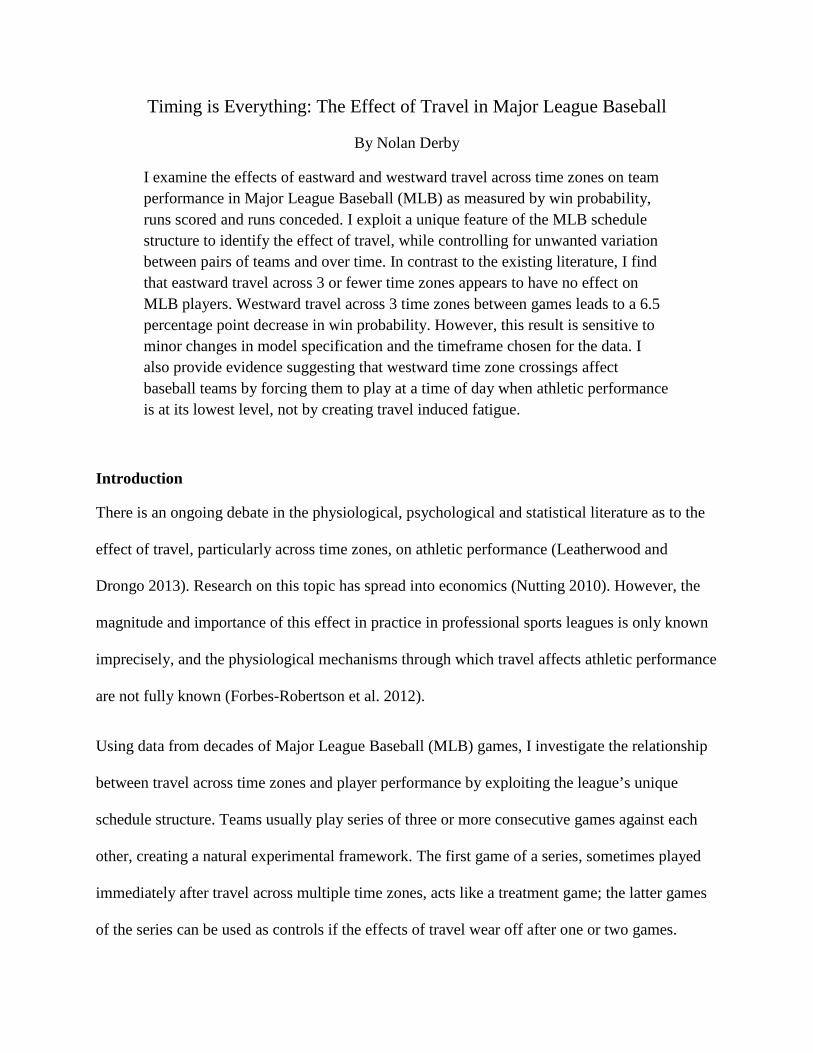
Timing is Everything: The Effect of Travel in Major League Baseball

By Nolan Derby

I examine the effects of eastward and westward travel across time zones on team performance in Major League Baseball (MLB) as measured by win probability, runs scored and runs conceded. I exploit a unique feature of the MLB schedule structure to identify the effect of travel, while controlling for unwanted variation between pairs of teams and over time. In contrast to the existing literature, I find that eastward travel across 3 or fewer time zones appears to have no effect on MLB players. Westward travel across 3 time zones between games leads to a 6.5 percentage point decrease in win probability. However, this result is sensitive to minor changes in model specification and the timeframe chosen for the data. I also provide evidence suggesting that westward time zone crossings affect baseball teams by forcing them to play at a time of day when athletic performance is at its lowest level, not by creating travel induced fatigue.

Introduction

There is an ongoing debate in the physiological, psychological and statistical literature as to the

effect of travel, particularly across time zones, on athletic performance (Leatherwood and

Drongo 2013). Research on this topic has spread into economics (Nutting 2010). However, the

magnitude and importance of this effect in practice in professional sports leagues is only known

imprecisely, and the physiological mechanisms through which travel affects athletic performance

are not fully known (Forbes-Robertson et al. 2012).

Using data from decades of Major League Baseball (MLB) games, I investigate the relationship

between travel across time zones and player performance by exploiting the league’s unique

schedule structure. Teams usually play series of three or more consecutive games against each

other, creating a natural experimental framework. The first game of a series, sometimes played

immediately after travel across multiple time zones, acts like a treatment game; the latter games

of the series can be used as controls if the effects of travel wear off after one or two games.

Using this within series approach to control for unwanted team pair and time variation, I find

evidence that travel has a statistically significant and negative effect on win probability, similar

in magnitude to the difference in win percentage between the top team in baseball and an average

team. However, this is only true for westward travel across three time zones—all other forms of

travel have no effect on win probabilities, runs scored or runs conceded—and the result is

sensitive to changes in model specification. Additionally, my results suggest that the effect of

travel on MLB teams is less severe and less precisely known than is suggested in previous papers

(Winter et al. 2009; Recht, Lew, and Schwartz 1995).

I also attempt to determine if my results provide support for either of two popular theories in the

physiological literature on athletic ability and travel by subjecting my preliminary results to

several extensions and robustness checks. I find little support for the theory that travel affects

MLB players by making them increasingly fatigued; however, I provide some evidence that

travel affects athletes by forcing them to effectively compete at a time of day associated with a

trough in human athletic performance (e.g. Kline et al. 2007).

Background Information

Major League Baseball is, since 1998, an organization of 30 professional teams, each of whom

plays a 162 game regular season schedule. 14 of these teams play in the Eastern Time Zone,

compared to 8 in the Central, 2 in the Mountain and 6 in the Pacific Time Zone. The first MLB

games were played in 1876, among 8 teams collectively known as the National League. Since

then, MLB has expanded, adding the American League in 1901 and increasing the number of

teams to 26 in 1977, 28 in 1994 and 30 between the 1997 and 1998 seasons. From 1998 to 2012,

these teams were organized into 2 and 6 divisions. Divisions are composed of teams from

similar, broad geographic areas; each team plays about half of its games against a division rival,

and about 80% of its remaining games against other teams in its same league.

No team has to travel more than two time zones from its home stadium to reach the home

stadium of any one of its division rivals. However, the American and National leagues both

contain multiple teams from the Eastern and Pacific Time Zones. Teams played at least two

series against every other team in their league in every year from 1998 to 2012. Therefore, I

observe hundreds of games in each season in which one team has travelled east or west across

multiple time zones between two games, while the other team has not crossed any time zones

during that same period.

Literature Review

The literature on the effect of travel on sports performance can be divided into several branches.

Physiological papers have subjected elite athletes to flights across multiple time zones, measured

their athletic performance using several tests every day after the flight for up to two weeks and

compared these performances to results obtained by the same athletes before travel. Lemmer et

al. (2002) separate members of the German Olympic Team onto two different flights: one

travelling east across eight time zones and the other travelling west across six time zones. The

authors find that both sets of athletes experience reduced grip strength, hormone levels, blood

pressure and heart rate for as long as seven days after travel. In a similar experiment, Reilly,

Atkinson and Budgett (2001) find that leg, back and grip strength and sleep quality and length

deteriorate on the first day after travel, and do not return to normal levels until five to seven days

after time zone crossings.

It should be noted, however, that athletes in North American professional sports leagues never

have to travel across more than three time zones at once between games. Since the marginal

effect of an additional time zone crossing on athletic performance is likely increasing in the

number of time zones crossed (Leatherwood and Drongo 2013), travel across three or fewer time

zones may have no effect on athletic performance. Physiological experiments of this nature may

provide suggestive evidence as to a negative effect of travel across time zones on elite athletic

performance. However, one might suspect that the adrenaline and higher stakes induced by a

competitive match produce a higher level of performance from elite athletes than tests conducted

in a controlled, laboratory setting.

A second branch of the literature has thus attempted to determine if the detrimental effects of

time zone crossings observed in closely monitored experiments are present in professional sports

leagues as well. For example, Nutting (2010) looks at the effect of travel on NBA teams, and

finds that westward travel across one or two time zones decreases win probabilities by about 7%,

but only in the second half of the season. Win probabilities also increase substantially in the

second half of the season for the team that enjoys the larger number of off days before a game,

leading the author to conclude that travel negatively affects NBA players by increasing fatigue.

In a review of existing research on travel and sports performance, Leatherwood and Drongo

(2013) note that an important, unanswered question in the literature is whether eastward and

westward travel have differential effects on elite athletes. Proponents of the theory that westward

travel has a larger effect than eastward travel on athletic performance in North American

professional sports leagues point out that games played in the Pacific Time Zone often begin at

6-7 PM local time, 9-10 PM Eastern Standard Time (EST), and often end 3 or more hours later.

Visiting players on an Eastern Time Zone team may therefore feel as though the game is actually

starting at 9-10 PM, and finishing at 12-1 AM. Several papers show that for elite athletes, leg and

back strength, and performance indicators like blood pressure and heart rate, are at their lowest

levels in the late evening and early morning and peak in the early to late afternoon (for a

comprehensive list, see Leatherwood and Drongo 2013). Therefore, Eastern teams may be at a

disadvantage when playing night games in the Pacific Time Zone. For the remainder of this

paper, I refer to this hypothesis as the “Effective Time Theory.”

A retrospective study of National Football League (NFL) games finds that West Coast teams

performed significantly better against East Coast teams than predicted by Las Vegas point

spreads in Monday Night Football games played over a 25 year period from 1970-1994 (Smith et

al. 1997). Since these games always started at 9:00 PM EST, regardless of their location, the

authors argue this is evidence for the Effective Time Theory. In a similar paper, Jehue et al.

(1993) also find that NFL teams experience a substantial increase in performance when playing

at an effective time of day in the late afternoon, early evening hours. Pacific Time Zone based

teams also enjoy a significant increase in win percentage above their average for the rest of the

season when playing in night games against teams from other time zones.

Kline et al. (2007) design an experiment in which elite swimmers were asked to perform 200

metre time trials at maximum effort at eight different 3 hour intervals, from 2 AM to 11 PM,

over the course of 50-55 hours, while being subjected to identical sleep schedules and other

environmental conditions. The authors find that swim times decrease by about 5 to 6 seconds

from a mean time of 169.5 seconds at 2 AM, 5 AM and 8 AM, but are otherwise quite similar.

Their results suggest a trough in athletic performance in very late evening, early morning hours.

Other physiological experiments and studies have concluded that eastward travel is more

detrimental than westward travel for elite athletic performance (e.g. Reilly 2009). The dominant

theory used to explain these results is that the human body can more easily adjust to eastward

travel, which lengthens the day, than westward travel, which shortens it (Leatherwood and

Drongo 2013; Loat and Rhodes 1989). More specifically, Manfredini et al. (1998) list several

physiological factors affecting athletic performance, including sleep quality and duration, which

are more negatively affected by eastward travel than westward travel. Reilly and Edwards (2009)

argue that athletes travelling east have fewer hours available to adjust to time zone transitions

through outdoor exercise during daylight hours, and find that sleep cycles take longer to recover

from eastward travel than westward travel. Evidence from these papers is compelling, but the

authors only study eastward travel across five or more time zones.

I argue that my results provide additional support for the Effective Time Theory, and find little

evidence that travel exacerbates fatigue experienced over the course of the gruelling 162 game

MLB schedule. However, baseball requires less anaerobic physical exertion than professional

sports like football and basketball. Travel induced fatigue may have a stronger impact on win

probabilities in more cardio intensive sports, as suggested by the results in Nutting (2010).

Papers on the Effect of Travel in Major League Baseball

Similar studies have also been conducted for Major League Baseball (MLB). To my knowledge,

Recht, Lew and Schwartz (1995) is the first article to look at the effect of travel across time

zones on win probabilities and runs scored in MLB. The authors look only at games in the 1991-

1993 seasons involving a team from the Pacific Time Zone and a team from the Eastern Time

Zone where one team had travelled across 3 time zones in the previous 3 days. They conclude

that travelling from the Pacific to Eastern Time Zone has a negative effect on win probability and

runs scored. Travel from the Eastern to Pacific Time Zone does not have a statistically

significant effect on win probability.

Winter et al. (2009), using data from the 1998 to 2007 seasons, find that travelling across three

time zones between games in less than 24 hours decreases win probability by 8.8 percentage

points. Both my paper and Winter et al. (2009) have a similar research question. However,

Winter et al. simply compare win percentages in these games with win percentages in games in

which neither team has just travelled across a time zone in the past 24 hours. In fact, neither

Winter et al. (2009) or Recht, Lew and Schwartz (1995) fully control for differences in team

quality, starting pitchers used for these games or other endogenous variables correlated with

travel distance. They obtain their results by simple OLS, using few or no controls. To deal with

these concerns, I propose an identification strategy to remove variation at the team pair, series

level. I also separate east and west travel in an attempt to provide additional evidence as to

whether or not the direction of time zone crossings influences athletic performance.

Data

I use game schedules for every MLB season from 1998, the first year after the league expanded

to its current number of 30 teams, to 2013 from the Retrosheet Database in my main

specifications. The Retrosheet Database provides runs scored and the name of the starting pitcher

for the home and visiting teams in every MLB game played after 1973, and the number of

pitchers used by each team in each game. Retrosheet also provides the date when each game was

played. From this information, I can infer if the home or visiting team enjoyed an off day before

every game, the travel schedules for each team in each MLB season, and the percentage of

games won by each team in each season.

To control for differences in the effectiveness of starting pitchers in each game, I use the starting

pitcher ID’s provided by Retrosheet in conjunction with data provided from the Lahman

Database on ERA; home runs, walks and hit by pitches allowed; innings pitched; and strikeouts

for every starting pitcher in MLB from 1977-2013. Tables 1.I and 1.II contain summary statistics

for the variables obtained from these two databases.

Econometric Model and Identification Strategy

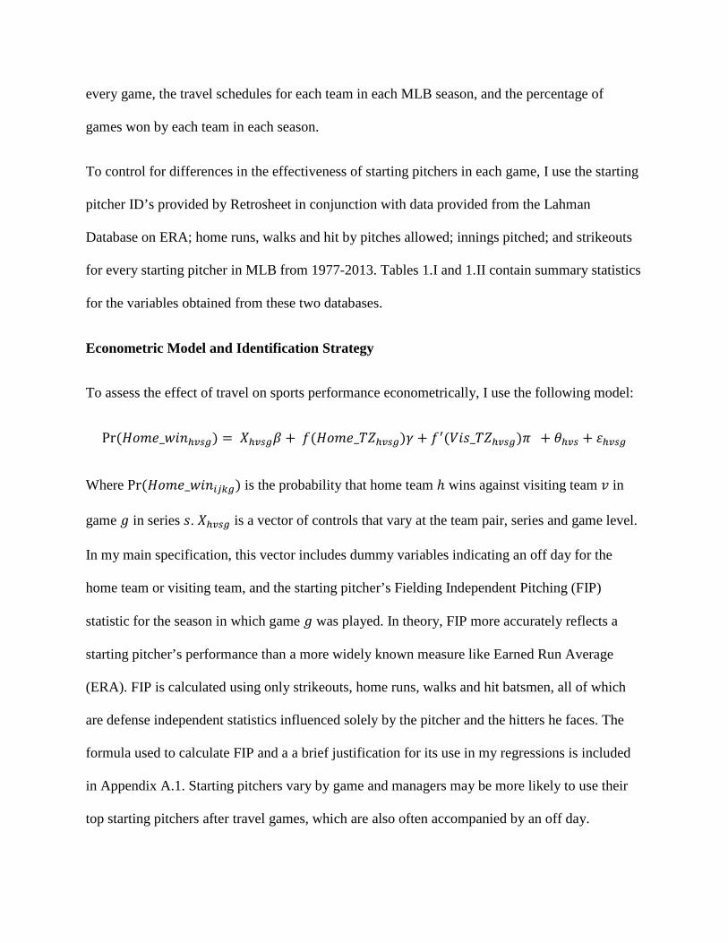
To assess the effect of travel on sports performance econometrically, I use the following model:

Pr (𝐻𝑜𝑚𝑒_𝑤𝑖𝑛ℎ𝑣𝑠𝑔) = 𝑋ℎ𝑣𝑠𝑔𝛽 + 𝑓(𝐻𝑜𝑚𝑒_𝑇𝑍ℎ𝑣𝑠𝑔)𝛾 + 𝑓′(𝑉𝑖𝑠_𝑇𝑍ℎ𝑣𝑠𝑔)𝜋 + 𝜃ℎ𝑣𝑠 + 𝜀ℎ𝑣𝑠𝑔

Where Pr (𝐻𝑜𝑚𝑒_𝑤𝑖𝑛𝑖𝑗𝑘𝑔) is the probability that home team ℎ wins against visiting team 𝑣 in

game 𝑔 in series 𝑠. 𝑋ℎ𝑣𝑠𝑔 is a vector of controls that vary at the team pair, series and game level.

In my main specification, this vector includes dummy variables indicating an off day for the

home team or visiting team, and the starting pitcher’s Fielding Independent Pitching (FIP)

statistic for the season in which game 𝑔 was played. In theory, FIP more accurately reflects a

starting pitcher’s performance than a more widely known measure like Earned Run Average

(ERA). FIP is calculated using only strikeouts, home runs, walks and hit batsmen, all of which

are defense independent statistics influenced solely by the pitcher and the hitters he faces. The

formula used to calculate FIP and a a brief justification for its use in my regressions is included

in Appendix A.1. Starting pitchers vary by game and managers may be more likely to use their

top starting pitchers after travel games, which are also often accompanied by an off day.

Therefore, I argue, it is important to control for the expected effectiveness of the starting pitcher

in each game.

I also observe the number of pitchers used by each team in each game, but I omit this variable

from my main specification; one effect of travel may be to tire out the starting pitcher and force

the travelling manager to use more relief pitchers than usual. In OLS estimations, I also control

for linear time trends by including a year variable as a regressor—important when runs scored is

used as a dependent variable, since offense has been trending downward since the 1998 season—

and the winning percentage of each team over the course of the season in which game 𝑔 was

played. 𝜃ℎ𝑣𝑠 represents fixed effects that vary at the team pair and series level. Eliminating this

term through my series fixed effects estimator is my preferred method of controlling for

confounding time and team pair variation.

𝑓(. ) and 𝑓′(. ) are functions of the number of time zones travelled by the home and visiting

teams respectively between games 𝑔 − 1 and 𝑔, and their coefficients 𝛾 and 𝜋 are my

parameters of interest. I distinguish between east and west time zone crossings by creating

separate dummy variables for east and west travel. Modelling 𝑓 and 𝑓′ in this way allows me to

account for the possibility that the relationship between time zone crossings and win probability

is non-linear and heterogeneous between east and west travel.

Over 90% of MLB series from 1998 to 2013 are 3 or more games in length. Thus, a simple

within-series differencing approach allows me to eliminate team pair, series fixed effects and

identify the effect of travel across time zones on win probability. I assume that any effects of

time zone crossings are present in the first and/or second games of a series, but are eliminated, or

at least mitigated, by the third and/or fourth games of the series. I later justify this assumption by

showing that any negative effects of time zone crossings are eliminated by the second game

played post-travel.

All of my results are obtained without clustered standard errors. However, if the error terms for

games within the same series are sometimes correlated, for example because one team is on a

“hot streak” and has a higher win probability during the series than its observable characteristics

would predict, then my standard errors are of the form 𝜀ℎ𝑣𝑠𝑔 = 𝛿ℎ𝑣𝑠 + 𝜖ℎ𝑣𝑠𝑔. In this case, I

should cluster my standard errors at the series level. However, Sire and Redner (2009) conclude

that MLB results over the past half century suggest that games are in fact independent, and that

the observed frequency and duration of winning and losing streaks are consistent with chance,

after conditioning on team ability. In light of this result, I refrain from clustering my standard

errors in my main specifications. Results obtained using standard errors clustered at the series

level are included in Appendix A.2. I also refrain from using heteroskedasticity robust standard

errors so that I can perform Hausman tests to check to see if OLS is consistent under the

hypothesis that my Series FE estimator is consistent, but show in Table A.2.1 that this has

virtually no effect on my main results.

Results:

I. Main Specification: The Effect of Travel on Win Probability

OLS regression of the model just described, using the post-expansion 1998 MLB season as my

start year, shows that win probability is affected by time zone crossings only when the home or

visiting team has travelled westward across 3 time zones between its current and previous games.

To interpret my results I define the effect size as the simple average of the coefficients on

westward travel across 3 time zones by the home and visiting teams, and test for joint

significance of these two variables using an F-test. This method implies that travel across three

time zones decreases the win probability of the travelling team by 4.1 percentage points in the

first game played post-travel, a result that is significant at the 10% level. After controlling for

series fixed effects, my preferred specification, the average effect size of westward travel across

3 time zones increases to 6.5 percentage points and is significant at the 5% level. Both my OLS

and Series FE estimates suggest that eastward travel across 3 time zones has no effect on win

probabilities. Table 2 contains full results.

II. The Effect of Travel on Position Players vs. Pitchers

Position players in MLB typically play almost every game of their team’s regular season

schedule and provide all of the offense for their teams. By contrast, the workload for a starting

pitcher is so intense that they rarely play more than once during any given 4 or 5 game stretch.

Relievers—pitchers who replace the starter during a game—are also usually given at least one

game off between appearances, in order to protect their throwing arms and prevent injury1. One

might expect then that travel has a relatively larger impact on position players: unlike most

pitchers, they do not have an opportunity to rest between games.

To test this hypothesis, I replace my dependent variable, winning percentage of the home team,

with runs scored by the home team and runs scored by the visiting team. I also control for the

total number of outs recorded in each game. This is important when runs scored by the home

team is used as the dependent variable, since the home team has 3 fewer outs with which to score

runs if it is leading after the top of the 9th inning. It is also possible that managers respond to the

negative effects of travel by using more pitchers than in a normal game. To account for this

1 Baseball Reference shows that from 1998-2010, relievers enjoyed at least one off day before pitching more than 75% of the time: Baseball Reference. 2011. “More pitching appearances are coming with zero days’ rest”. February 23. http://www.baseball-reference.com/blog/archives/10071

possibility, I include number of pitchers used by the visiting and home teams as additional

controls as well.

If travel does negatively affect position players, the magnitude of the coefficient on westward

travel across three time zones for the home team should be negative when runs scored by the

home team is the dependent variable. If teams concede more runs in games played post-travel,

then the coefficients on indicators for travel by the home team should be positive when visiting

team runs scored is the dependent variable. Analogous statements of course hold if runs scored

by the visiting team is used as the dependent variable instead.

The results, shown in Table 4, suggest that runs scored by the visiting team decrease by about

-0.33 runs per game in the team’s first game played after travelling west across three time zones.

The coefficient on the indicator for the home team travelling west across three time zones is

about 0.23, but insignificant. However, an F-test shows that the hypothesis that these two

coefficients are equal to one another cannot be rejected. Similar results are obtained when runs

scored by the home team is used as a dependent variable; therefore, there is no evidence that

travel across three time zones has a more negative effect on position players than pitchers.

Surprisingly, home teams also appear to score an additional 0.33 runs per game when the visiting

team has travelled east across three time zones before a game, a result that is significant at the

5% level. My earlier results imply that visiting team win probability and runs scored do not

change after such travel, even though the average home and visiting team run differential for

games played after 1998 is only 0.13 runs and 28% of games over this timeframe were decided

by one run. Eastward travel across three time zones by the home team also appears to have no

effect on runs scored by the visiting team, as shown in Table 4. In light of these other results

indicating that eastward travel does not affect MLB players, I treat the apparent relationship

between eastward travel by the visiting team across three time zones and runs scored by the

home team as anomalous. Overall, I conclude that travel does not appear to have differential

effects on position players and pitchers.

III. Interpretation of Results and Comparison to the Existing Literature

Previous papers that have studied the effects of travel across 3 time zones on win probabilities

and scoring in Major League Baseball have concluded that the effect of such travel is substantial

and highly significant. Recht, Lew and Schwartz (1995) find, using data from 1991 to 1993, that

teams based in the Eastern Time Zone score 1.24 more runs per game and are 8.8 percentage

points more likely to win when hosting an opponent that has just travelled east three time zones.

Their results show no effect of travel when the home team instead has travelled east across three

time zones. My results in Table 2 suggest that both of these numbers are strongly influenced by

the authors’ choice of seasons. When looking at games played from 1998 to 2013, eastward

travel by the visiting team across three time zones increases runs scored by the home team by

only 0.4 runs per game, and has no statistically significant effect on win percentage.

Furthermore, if eastward travel across three time zones really does have a negative effect on run

production, it is not clear why this relationship should hold for only visiting teams. Results from

both my paper and Recht, Lew and Schwartz (1995) show that teams returning from the Pacific

Time Zone to host a game in the Eastern Time Zone are unaffected by such travel.

Winter et al. (2009) find, using data from 1997-2006, that travel across three time zones, by the

home or visiting team, decreases the win probability of the travelling team by 8.8 percentage

points. While the authors also conclude that westward travel has a stronger effect than eastward

travel, their results suggest that crossing three time zones in either direction significantly affects

win percentage. By contrast, I find, using an expanded 1998-2013 dataset, that only westward

travel had any significant effect on win probability. Full results are available in Table 2. The

average effect of such travel by the home and visiting teams on win probability decreases from

8.8 percentage points to 6.5 percentage points when controlling for series fixed effects, and to

4.1 percentage points when using OLS.

Using 1998, the year of the last MLB expansion, as my own cut-off year is still somewhat

arbitrary, as MLB has featured both a 162 game schedule and teams located in both the Eastern

and Pacific Time Zones since 1962. From 1977, the year after MLB expanded from 24 to 26

teams, to 2013, westward travel across three time zones decreases win probability in the first

game played post-travel by only 3.6 percentage points when controlling for series fixed effects,

and 3.0 percentage points using OLS. Table 3 contains full results. Furthermore, the coefficients

become jointly significant at the 10% level or just above it when using OLS or series fixed

effects estimates, despite the addition of 21 years’ worth of data.

I still prefer using 1998 as the cut-off year in most of my specifications, as changes in scheduling

format, improvements in average player quality and training, and different rest schedules for

starting pitchers since the 1970s and 1980s may have altered the effects of travel in ways that I

cannot control for or observe. One might expect though, given increases in player salary and

scientific knowledge about how to counteract the effects of jet lag over time that MLB players

have become better at dealing with travel in more recent years. If the effect of travel across three

time zones on MLB players is as substantial as suggested in Recht, Lew and Schwartz (1995)

and Winter et al. (2009), it is difficult to explain why the impact of travel on win probability and

runs scored in MLB decreases as I increase the number of seasons included in my data set.

Therefore, I attempt to determine if travel has any effect on MLB players by running several

additional regressions motivated by physiological theories on the relationship between travel and

athletic performance.

Extensions

IV. The Effect of Travel at Night and During Long Games

As mentioned, there remains debate in the literature as to whether or not eastward or westward

travel has a stronger impact on athletic performance in North American professional sports

leagues. The Effective Time Theory, based on evidence that athletic performance is at its lowest

level in late evening, early morning hours, is the favoured explanation for those who believe that

westward travel is more detrimental.

Just over two-thirds of MLB games from 1998-2013 were played at night, with the vast majority

of these games starting at 7:00 PM local time. The remaining third were played during the day,

usually starting at either 11:30 AM or 2:30 PM local time. Ideally, I would like to see if the

negative effects of westward travel across three time zones are exacerbated in night games, when

the team travelling from the Eastern Time Zone is playing in a game starting at 10 PM EST.

However, since 1998, only 15 day games have been played after the home or visiting team has

just travelled west across 3 time zones, compared to 674 night games meeting the same criteria.

My later results suggest full acclimation to westward travel across 3 time zones takes only 1

game, so the lack of day games post cross-country travel makes it difficult to determine if the

Effective Time Theory can explain the negative effect of westward travel. However, I do observe

the length, in minutes of each game in my data set, which provides me with an alternative means

to test this theory. I interact an indicator variable for travel across 2 time zones by the home or

visiting team before the game with an indicator for the game being above mean length of 175

minutes and played at night to see if westward travel across two time zones has a negative effect

in long games. To control for the possibility that travelling teams perform worse in long games

because of fatigue, I add the same interactions terms for travel across three time zones as well.

As predicted by the Effective Time Theory, home winning percentage increases by about 7.1

percentage points in long, night games in which the visiting team has travelled west across two

time zones, and decreases by 15 percentage points in such games when the home team has

travelled west across two time zones instead. F tests show that these coefficients are jointly

different from zero at the 5% level, and different from visiting and home team winning

percentages in other games in which westward travel across two time zones occurred beforehand.

The same interaction terms for westward travel across three time zones, and eastward travel

across two and three time zones, are not significant jointly or on their own. These results suggest

that the Effective Time Theory explains the negative effect of westward travel across two time

zones in long, night games. Table 5 contains full results.

V. Testing for Travel Persistence over More than One Game

My analysis up to this point has assumed that the negative effects of westward travel across three

time zones last for only one game. Since approximately 90% of all MLB series played since

1998 consisted of three or more games, my data set allows me to test the possibility that travel

effects persist into the second game as well using my series FE estimator. To do this, I generate

two binary variables: one indicates eastward or westward travel across three time zones between

the current and previous game, while the other indicates the same type of travel between the

previous game, and the game before that. The third game of the series is then effectively the

control game (along with the fourth and fifth games of the series, if played).

My results suggest westward travel across three time zones is, in fact, only detrimental in the

first game played after the time zone crossings. Using my series FE estimator I find that home

win percentage does not change significantly in the second game played after travel, regardless

of whether the home or visiting team travelled prior to the series. To control for the possibility

that travel across three time zones lasts for more than two games, but is felt most strongly in the

first game post travel, I run the same estimation using OLS, again controlling for both teams’

win percentage over the course of the season in place of series fixed effects. Again, I find that

crossing three time zones only has a statistically significant effect on win percentage in the first

game played post-travel. Result tables are available in Appendix A.3.

VI. Travel, Fatigue and the 2006 Amphetamine Ban

It is well documented that MLB was suffering from a performance enhancing drug problem in

the 1990s and early 2000s. Included among these substances is a class of drugs known as

amphetamines, which increase energy levels before games and combat the inevitable fatigue that

arises during a gruelling MLB schedule requiring teams to play 162 games in 180 days. MLB

banned amphetamines before the start of the 2006 season, which may have increased the

negative effects of travel on performance. To test this possibility, I add interaction terms

identifying post-2005 games in which one team has travelled across three time zones since their

previous game.

Despite anecdotal evidence from former MLB players and medical experts involved with the

league that amphetamine usage was rampant before the 2006 ban2, I find no evidence that travel

has a more negative effect on performance in games played after 2006. The coefficients on the

post-2006, westward travel across three time zones terms are both insignificant, on their own and

jointly in an F-test. Furthermore, coefficients on the post-2006 interaction terms often have the

opposite sign expected if the amphetamine ban increased travel related fatigue.

One possibility, suggested by Will Carroll3, a noted author on the use of performance enhancing

substances in Major League Baseball, and the New York Times4 is that players successfully

substituted away from amphetamines to similar substances after the 2006 amphetamine ban.

Alternatively, many players may still be using amphetamines, in violation of the League’s drug

policy. Therefore, I use an alternative test to see if travel affects players by making them

increasingly more fatigued: I interact my standard travel variable with a binary variable

indicating a game played in the second half of the season. If travel does affect players by making

them more tired, then the data should show that the decrease in win probability after travel across

three time zones is greater in the second half than in the first half of the season. However, results

in Appendix A.4 show that I cannot reject the hypothesis that the effects of travel across three

time zones are constant throughout the season.

Conclusion

Contrary to findings in previous papers studying the effect of travel on team performance in

MLB, this paper shows that eastward travel across three time zones appears to have no effect on

2 Carroll, Will. 2006. “Under the Knife: Amphetamines and Baseball.” Baseball Prospectus, February 2. http://www.baseballprospectus.com/article.php?articleid=4740 3 Ibid. 4 Curry, Jack. 2006. “With Greenies Banned, Up for a Cup of Coffee?” New York Times, April 1. http://www.nytimes.com/2006/04/01/sports/baseball/01greenies.html?pagewanted=all&_r=1&

win probability or run production. Westward travel across three time zones leads to an estimated

6.5 percentage point decrease in win probability in the next game played by the travelling team,

though this effect size decreases to 3.6 percentage points when I use 1977 instead of 1998 as the

start year for my data set. These results, coupled with my finding that westward travel across two

time zones also has a negative effect on win probability in long, night games played post-travel,

suggest that professional MLB players suffer from travel only when it forces them to play in late

evening, early morning hours before becoming accustomed to a time zone change. By contrast, I

find no evidence to support the hypothesis that travel affects MLB players by intensifying

fatigue. Viewed in the context of the broader literature, my overall results add to a growing body

of literature suggesting that elite athletes suffer a decline in performance when forced to play

games in the late evening or early morning. However, future research is needed to determine

when and if the negative, fatiguing effects of travel on athletic performance observed in

controlled laboratory settings manifest themselves in other professional sports leagues.

References

Forbes-Robertson, Sarah, Edward Dudley, Pankaj Vadgama, Christian Cook, Scott Drawer, and Liam Kilduff. 2012. “Circadian Disruptions and Remedial Interventions.” Sports Medicine 42(3): 185-208. Jehue, Richard, David Street, and Robert Huizenga. 1993. “Effect of time zone and game time changes on team performance: National Football League.” Medicine and Science in Sports and Exercise 25(1) 127-131. Kline, Christopher E., J. Larry Durstine, J. Mark Davis, Teresa A. Moore, Tina M. Devlin, Mark R. Zielinski, and Shawn D. Youngstedt. 2007. “Circadian variation in swim performance.” Journal of Applied Physiology 102: 641-649. Lahman, Sean. 2013. “Lahman’s Baseball Database.” http://www.seanlahman.com/baseball-archive/statistics/ (accessed July 30, 2014). Leatherwood, Whitney E., and Jason L Dragoo. 2013. “Effect of airline travel on performance: a review of the literature.” British Journal of Sports Medicine 47 (9): 561-567. Lemmer, Bjorn, Ralph-Ingo Kern, Gudrun Nold, and Heinz Lohrer. 2002. “Jet lag in athletes after eastward and westward time-zone transition”. Chronobiology International 19(4): 743-764. Loat, C.E.R., and E.C. Rhodes. 1989. “Jet-lag and human performance.” Sports Medicine 8(4): 226-238. Manfredini, Roberto, Fabio Manfredini, Carmelo Fersini, and Francesco Conconi. 1998. British Journal of Sports Medicine 32(2) 101-106. Nutting, Andrew W. 2010. “Travel costs in the NBA production function.” Journal of Sports Economics 11(5) 533-548. Recht, Lawrence D., Robert A. Lew, and William J. Schwartz (1995). “Baseball teams beaten by jet lag.” Nature 377: 583.

Reilly, Thomas. 2009. “How can travelling athletes deal with jet-lag?” Kinesiology 41(2): 128-135.

Reilly, Thomas, and Ben Edwards. 2007. “Altered sleep-wake cycles and physical performance in athletes.” Physiology and Behavior 90(2-3): 274-284.

Reilly, Thomas., Greg Atkinson, and Richard Budgett. 2001. “Effect of Low-Dose Temazepam on Physiological Variables and Performance Tests Following a Westerly Flight Across Five Time Zones.” International Journal of Sports Medicine 22(3): 166-174.

Sire, Clément, and Sidney Redner. 2009. “Understanding baseball team standings and streaks.” The European Physical Journal B-Condensed Matter 67(3): 473-481.

Smith, David W. 1989. “Retrosheet Game Logs 1977-2013”. Retrosheet. http://www.retrosheet.org/gamelogs/index.html (accessed July 30, 2014). Smith, Roger S., Christian Guilleminault, and Bradley Efron. 1997. “Circadian Rhythms and Enhanced Athletic Performance in the National Football League.” Sleep 20(5): 362-365. Winter, Christopher W., William R. Hammond, Noah H. Green, Zhiyong Zhang and Donald L. Bilwise. 2009. “Measuring circadian advantage in baseball: a 10-year retrospective study” International Journal of Sports Physiology and Performance 4(3): 394-401.

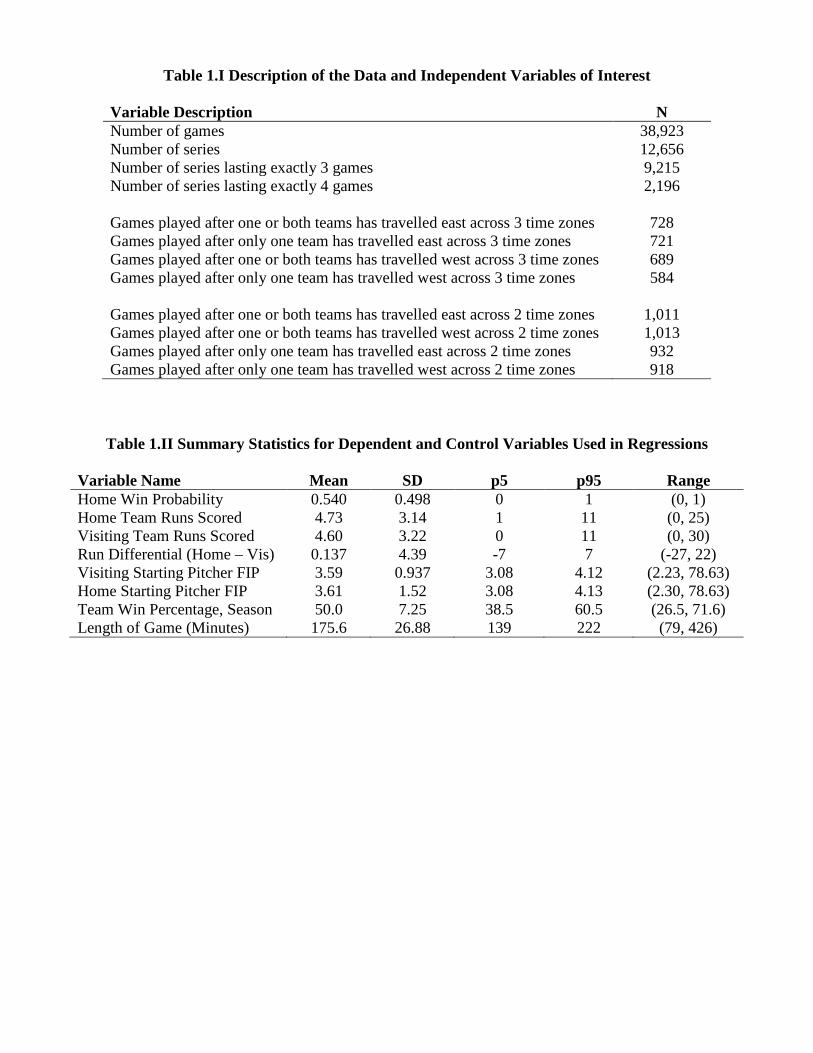
Table 1.I Description of the Data and Independent Variables of Interest

Variable Description N Number of games 38,923 Number of series 12,656 Number of series lasting exactly 3 games 9,215 Number of series lasting exactly 4 games 2,196 Games played after one or both teams has travelled east across 3 time zones

728

Games played after only one team has travelled east across 3 time zones 721 Games played after one or both teams has travelled west across 3 time zones 689 Games played after only one team has travelled west across 3 time zones 584 Games played after one or both teams has travelled east across 2 time zones

1,011

Games played after one or both teams has travelled west across 2 time zones 1,013 Games played after only one team has travelled east across 2 time zones 932 Games played after only one team has travelled west across 2 time zones 918

Table 1.II Summary Statistics for Dependent and Control Variables Used in Regressions

Variable Name Mean SD p5 p95 Range Home Win Probability 0.540 0.498 0 1 (0, 1) Home Team Runs Scored 4.73 3.14 1 11 (0, 25) Visiting Team Runs Scored 4.60 3.22 0 11 (0, 30) Run Differential (Home – Vis) 0.137 4.39 -7 7 (-27, 22) Visiting Starting Pitcher FIP 3.59 0.937 3.08 4.12 (2.23, 78.63) Home Starting Pitcher FIP 3.61 1.52 3.08 4.13 (2.30, 78.63) Team Win Percentage, Season 50.0 7.25 38.5 60.5 (26.5, 71.6) Length of Game (Minutes) 175.6 26.88 139 222 (79, 426)

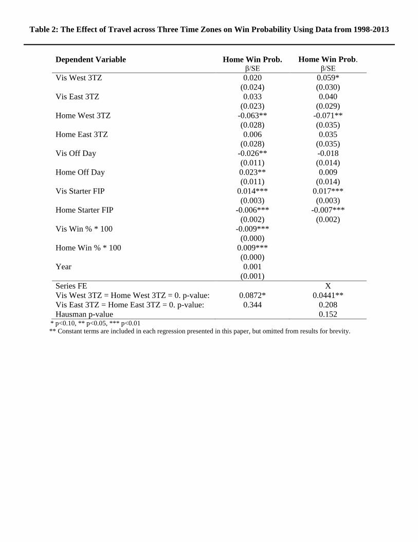
Table 2: The Effect of Travel across Three Time Zones on Win Probability Using Data from 1998-2013

Dependent Variable Home Win Prob. β/SE

Home Win Prob. β/SE

Vis West 3TZ 0.020 0.059* (0.024) (0.030) Vis East 3TZ 0.033 0.040 (0.023) (0.029) Home West 3TZ -0.063** -0.071** (0.028) (0.035) Home East 3TZ 0.006 0.035 (0.028) (0.035) Vis Off Day -0.026** -0.018 (0.011) (0.014) Home Off Day 0.023** 0.009 (0.011) (0.014) Vis Starter FIP 0.014*** 0.017*** (0.003) (0.003) Home Starter FIP -0.006*** -0.007*** (0.002) (0.002) Vis Win % * 100 -0.009*** (0.000) Home Win % * 100 0.009*** (0.000) Year 0.001 (0.001) Series FE Vis West 3TZ = Home West 3TZ = 0. p-value:

0.0872*

X 0.0441**

Vis East 3TZ = Home East 3TZ = 0. p-value: 0.344 0.208 Hausman p-value 0.152

* p<0.10, ** p<0.05, *** p<0.01 ** Constant terms are included in each regression presented in this paper, but omitted from results for brevity.

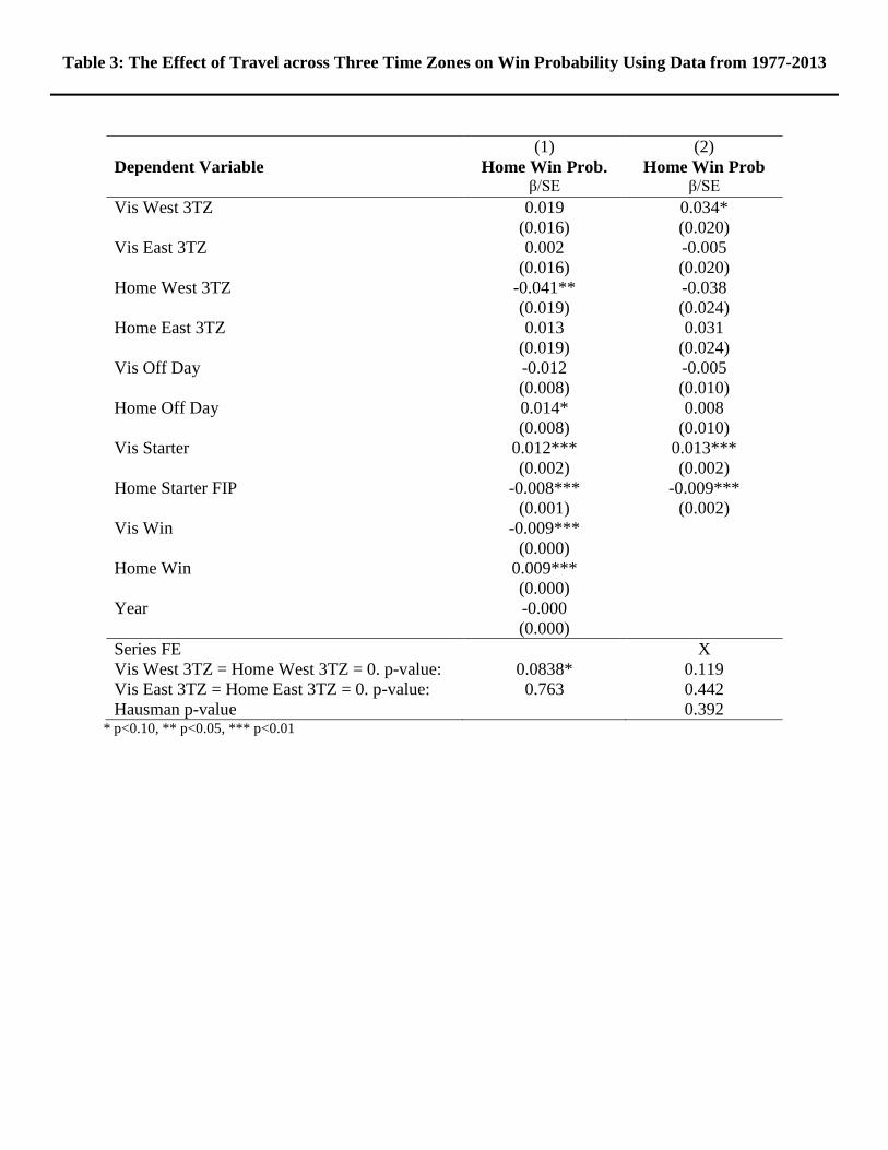
Table 3: The Effect of Travel across Three Time Zones on Win Probability Using Data from 1977-2013

(1) (2) Dependent Variable Home Win Prob. Home Win Prob β/SE β/SE Vis West 3TZ 0.019 0.034* (0.016) (0.020) Vis East 3TZ 0.002 -0.005 (0.016) (0.020) Home West 3TZ -0.041** -0.038 (0.019) (0.024) Home East 3TZ 0.013 0.031 (0.019) (0.024) Vis Off Day -0.012 -0.005 (0.008) (0.010) Home Off Day 0.014* 0.008 (0.008) (0.010) Vis Starter 0.012*** 0.013*** (0.002) (0.002) Home Starter FIP -0.008*** -0.009*** (0.001) (0.002) Vis Win -0.009*** (0.000) Home Win 0.009*** (0.000) Year -0.000 (0.000) Series FE Vis West 3TZ = Home West 3TZ = 0. p-value:

0.0838*

X 0.119

Vis East 3TZ = Home East 3TZ = 0. p-value: 0.763 0.442 Hausman p-value 0.392

* p<0.10, ** p<0.05, *** p<0.01

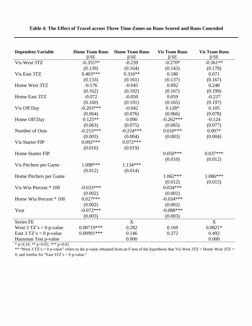
Table 4: The Effect of Travel across Three Time Zones on Runs Scored and Runs Conceded

Dependent Variable Home Team Runs β/SE

Home Team Runs β/SE

Vis Team Runs β/SE

Vis Team Runs β/SE

Vis West 3TZ -0.355** -0.239 -0.270* -0.361** (0.139) (0.164) (0.143) (0.170) Vis East 3TZ 0.403*** 0.316** 0.180 0.071 (0.133) (0.161) (0.137) (0.167) Home West 3TZ -0.176 -0.045 0.092 0.248 (0.162) (0.192) (0.167) (0.199) Home East 3TZ -0.072 -0.050 0.059 -0.227 (0.160) (0.191) (0.165) (0.197) Vis Off Day -0.203*** -0.042 0.128* 0.105 (0.064) (0.076) (0.066) (0.078) Home Off Day 0.125** 0.090 -0.262*** -0.124 (0.063) (0.075) (0.065) (0.077) Number of Outs -0.215*** -0.224*** 0.010*** 0.007* (0.003) (0.004) (0.003) (0.004) Vis Starter FIP 0.092*** 0.072*** (0.016) (0.019) Home Starter FIP 0.050*** 0.037*** (0.010) (0.012) Vis Pitchers per Game 1.098*** 1.134*** (0.012) (0.014) Home Pitchers per Game 1.062*** 1.086*** (0.012) (0.015) Vis Win Percent * 100 -0.033*** 0.034*** (0.002) (0.002) Home Win Percent * 100 0.027*** -0.034*** (0.002) (0.002) Year -0.072*** -0.088*** (0.003) (0.003) Series FE West 3 TZ’s = 0 p-value

0.00719***

X 0.282

0.169

X 0.0821*

East 3 TZ’s = 0 p-value 0.00991*** 0.146 0.372 0.492 Hausman Test p-value 0.000 0.000 * p<0.10, ** p<0.05, *** p<0.01 ** “West 3 TZ’s = 0 p-value” refers to the p-value obtained from an F-test of the hypothesis that Vis West 3TZ = Home West 3TZ = 0, and similar for “East 3TZ’s = 0 p-value.”

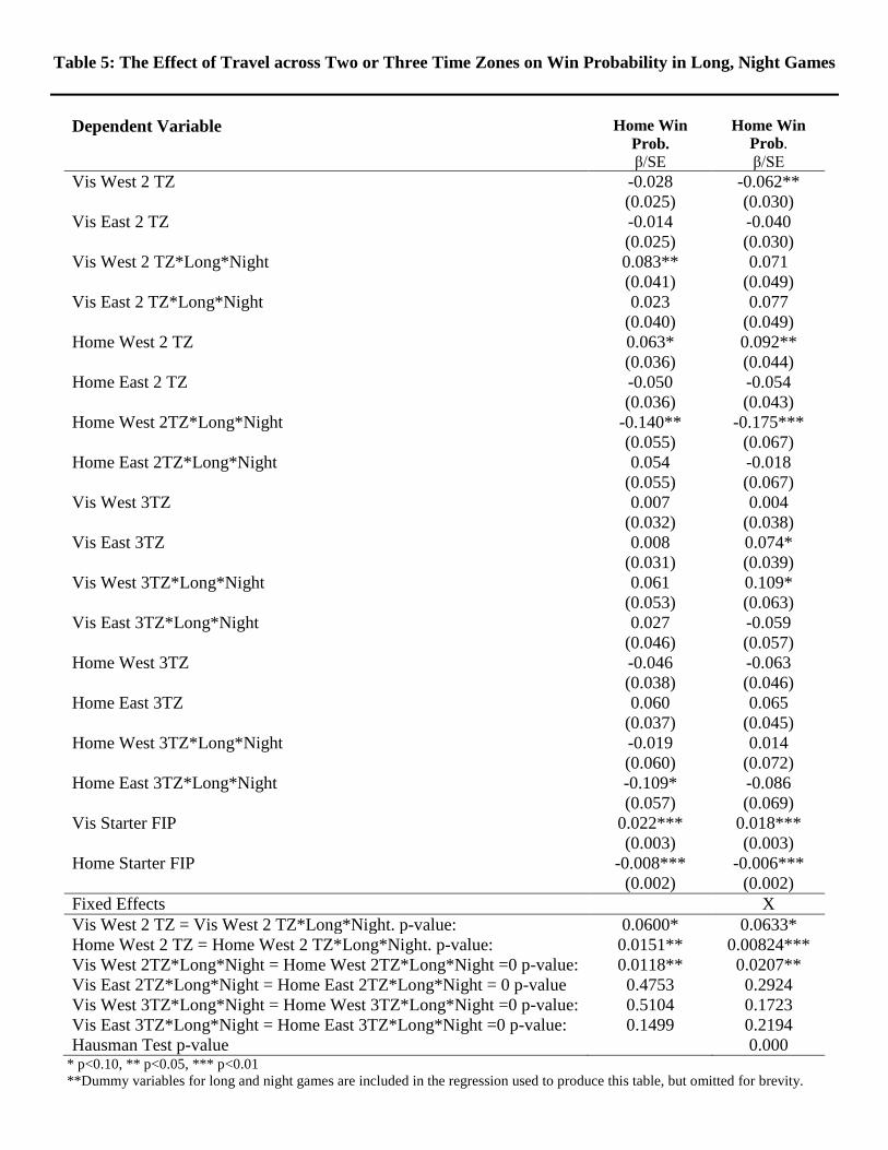
Table 5: The Effect of Travel across Two or Three Time Zones on Win Probability in Long, Night Games

Dependent Variable Home Win

Prob. β/SE

Home Win Prob. β/SE

Vis West 2 TZ -0.028 -0.062** (0.025) (0.030) Vis East 2 TZ -0.014 -0.040 (0.025) (0.030) Vis West 2 TZ*Long*Night 0.083** 0.071 (0.041) (0.049) Vis East 2 TZ*Long*Night 0.023 0.077 (0.040) (0.049) Home West 2 TZ 0.063* 0.092** (0.036) (0.044) Home East 2 TZ -0.050 -0.054 (0.036) (0.043) Home West 2TZ*Long*Night -0.140** -0.175*** (0.055) (0.067) Home East 2TZ*Long*Night 0.054 -0.018 (0.055) (0.067) Vis West 3TZ 0.007 0.004 (0.032) (0.038) Vis East 3TZ 0.008 0.074* (0.031) (0.039) Vis West 3TZ*Long*Night 0.061 0.109* (0.053) (0.063) Vis East 3TZ*Long*Night 0.027 -0.059 (0.046) (0.057) Home West 3TZ -0.046 -0.063 (0.038) (0.046) Home East 3TZ 0.060 0.065 (0.037) (0.045) Home West 3TZ*Long*Night -0.019 0.014 (0.060) (0.072) Home East 3TZ*Long*Night -0.109* -0.086 (0.057) (0.069) Vis Starter FIP 0.022*** 0.018*** (0.003) (0.003) Home Starter FIP -0.008*** -0.006*** (0.002) (0.002) Fixed Effects X Vis West 2 TZ = Vis West 2 TZ*Long*Night. p-value: 0.0600* 0.0633* Home West 2 TZ = Home West 2 TZ*Long*Night. p-value: Vis West 2TZ*Long*Night = Home West 2TZ*Long*Night =0 p-value: Vis East 2TZ*Long*Night = Home East 2TZ*Long*Night = 0 p-value Vis West 3TZ*Long*Night = Home West 3TZ*Long*Night =0 p-value: Vis East 3TZ*Long*Night = Home East 3TZ*Long*Night =0 p-value:

0.0151** 0.0118** 0.4753 0.5104 0.1499

0.00824*** 0.0207** 0.2924 0.1723 0.2194

Hausman Test p-value 0.000 * p<0.10, ** p<0.05, *** p<0.01 **Dummy variables for long and night games are included in the regression used to produce this table, but omitted for brevity.

Appendices

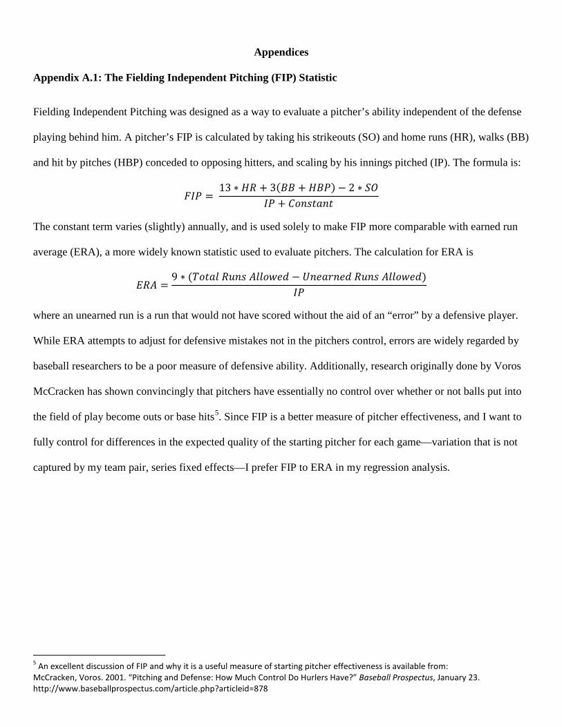
Appendix A.1: The Fielding Independent Pitching (FIP) Statistic

Fielding Independent Pitching was designed as a way to evaluate a pitcher’s ability independent of the defense

playing behind him. A pitcher’s FIP is calculated by taking his strikeouts (SO) and home runs (HR), walks (BB)

and hit by pitches (HBP) conceded to opposing hitters, and scaling by his innings pitched (IP). The formula is:

𝐹𝐼𝑃 = 13 ∗ 𝐻𝑅 + 3(𝐵𝐵 + 𝐻𝐵𝑃) − 2 ∗ 𝑆𝑂

𝐼𝑃 + 𝐶𝑜𝑛𝑠𝑡𝑎𝑛𝑡

The constant term varies (slightly) annually, and is used solely to make FIP more comparable with earned run

average (ERA), a more widely known statistic used to evaluate pitchers. The calculation for ERA is

𝐸𝑅𝐴 =9 ∗ (𝑇𝑜𝑡𝑎𝑙 𝑅𝑢𝑛𝑠 𝐴𝑙𝑙𝑜𝑤𝑒𝑑 − 𝑈𝑛𝑒𝑎𝑟𝑛𝑒𝑑 𝑅𝑢𝑛𝑠 𝐴𝑙𝑙𝑜𝑤𝑒𝑑)

𝐼𝑃

where an unearned run is a run that would not have scored without the aid of an “error” by a defensive player.

While ERA attempts to adjust for defensive mistakes not in the pitchers control, errors are widely regarded by

baseball researchers to be a poor measure of defensive ability. Additionally, research originally done by Voros

McCracken has shown convincingly that pitchers have essentially no control over whether or not balls put into

the field of play become outs or base hits5. Since FIP is a better measure of pitcher effectiveness, and I want to

fully control for differences in the expected quality of the starting pitcher for each game—variation that is not

captured by my team pair, series fixed effects—I prefer FIP to ERA in my regression analysis.

5 An excellent discussion of FIP and why it is a useful measure of starting pitcher effectiveness is available from: McCracken, Voros. 2001. “Pitching and Defense: How Much Control Do Hurlers Have?” Baseball Prospectus, January 23. http://www.baseballprospectus.com/article.php?articleid=878

Appendix A.2: Clustered and Heteroskedasticity Robust Standard Errors

Throughout this paper, I use errors that are not robust to heteroskedasticity, so that I can perform Hausman tests

to determine if my series FE estimator is eliminating meaningful variation, and refrain from clustering my

standard errors. Allowing for heteroskedasticity robust standard errors has essentially zero effect on the p-

values that I obtain for my coefficients of interest in any of the regressions performed in my paper. However,

despite the findings in Sire and Redner (2009) that MLB games are independent, clustering standard errors at

the series or team pair level when I control for series fixed effects often implies that my coefficients of interest

are only significant at the 10% level or just above it instead of the 5% level. This is likely because I lose over

12,000 degrees of freedom relative to OLS when I control for series fixed effects, and I am identifying the

effects of westward travel from about 2% of my observations as shown in Table 1I. Table A.2.1 below

illustrates this point for my results from my regressions with home win probability as my dependent variable:

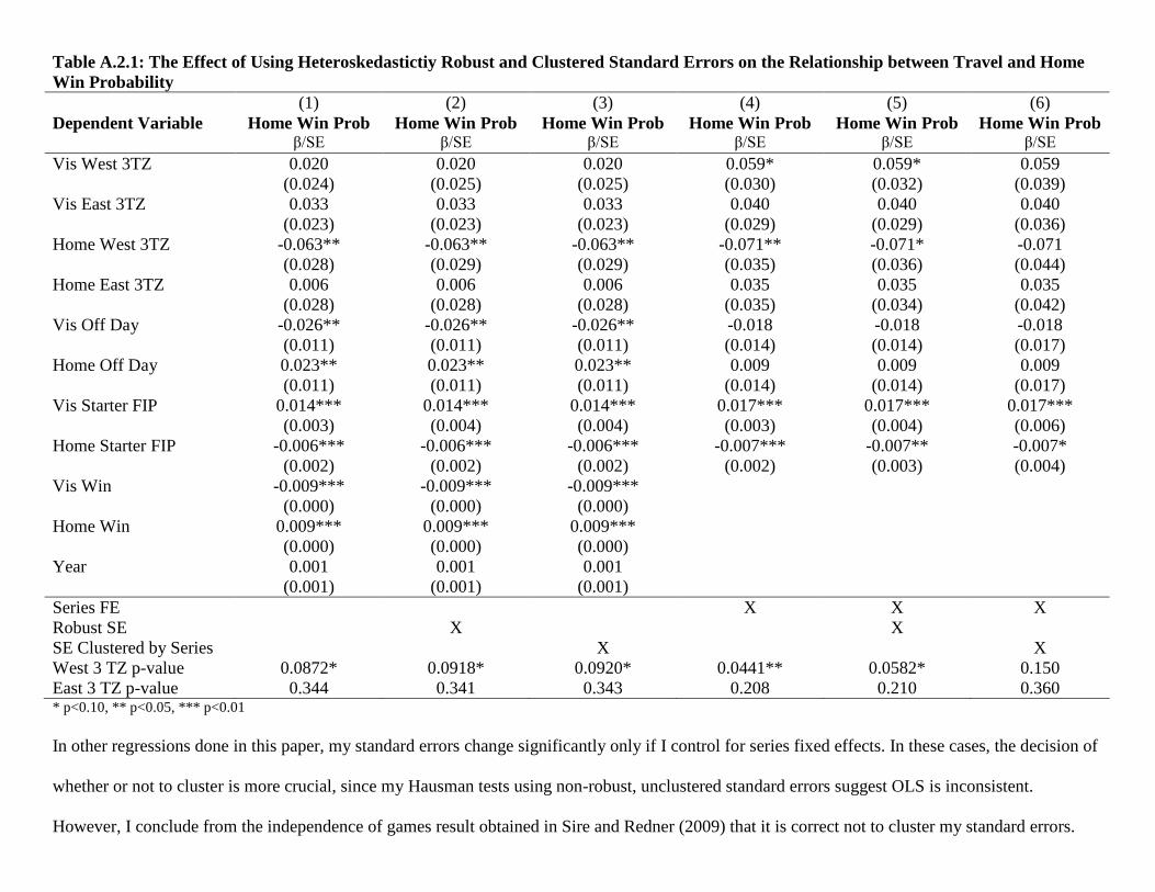
Table A.2.1: The Effect of Using Heteroskedastictiy Robust and Clustered Standard Errors on the Relationship between Travel and Home Win Probability (1) (2) (3) (4) (5) (6) Dependent Variable Home Win Prob Home Win Prob Home Win Prob Home Win Prob Home Win Prob Home Win Prob β/SE β/SE β/SE β/SE β/SE β/SE Vis West 3TZ 0.020 0.020 0.020 0.059* 0.059* 0.059 (0.024) (0.025) (0.025) (0.030) (0.032) (0.039) Vis East 3TZ 0.033 0.033 0.033 0.040 0.040 0.040 (0.023) (0.023) (0.023) (0.029) (0.029) (0.036) Home West 3TZ -0.063** -0.063** -0.063** -0.071** -0.071* -0.071 (0.028) (0.029) (0.029) (0.035) (0.036) (0.044) Home East 3TZ 0.006 0.006 0.006 0.035 0.035 0.035 (0.028) (0.028) (0.028) (0.035) (0.034) (0.042) Vis Off Day -0.026** -0.026** -0.026** -0.018 -0.018 -0.018 (0.011) (0.011) (0.011) (0.014) (0.014) (0.017) Home Off Day 0.023** 0.023** 0.023** 0.009 0.009 0.009 (0.011) (0.011) (0.011) (0.014) (0.014) (0.017) Vis Starter FIP 0.014*** 0.014*** 0.014*** 0.017*** 0.017*** 0.017*** (0.003) (0.004) (0.004) (0.003) (0.004) (0.006) Home Starter FIP -0.006*** -0.006*** -0.006*** -0.007*** -0.007** -0.007* (0.002) (0.002) (0.002) (0.002) (0.003) (0.004) Vis Win -0.009*** -0.009*** -0.009*** (0.000) (0.000) (0.000) Home Win 0.009*** 0.009*** 0.009*** (0.000) (0.000) (0.000) Year 0.001 0.001 0.001 (0.001) (0.001) (0.001) Series FE X X X Robust SE X X SE Clustered by Series X X West 3 TZ p-value 0.0872* 0.0918* 0.0920* 0.0441** 0.0582* 0.150 East 3 TZ p-value 0.344 0.341 0.343 0.208 0.210 0.360 * p<0.10, ** p<0.05, *** p<0.01 In other regressions done in this paper, my standard errors change significantly only if I control for series fixed effects. In these cases, the decision of

whether or not to cluster is more crucial, since my Hausman tests using non-robust, unclustered standard errors suggest OLS is inconsistent.

However, I conclude from the independence of games result obtained in Sire and Redner (2009) that it is correct not to cluster my standard errors.

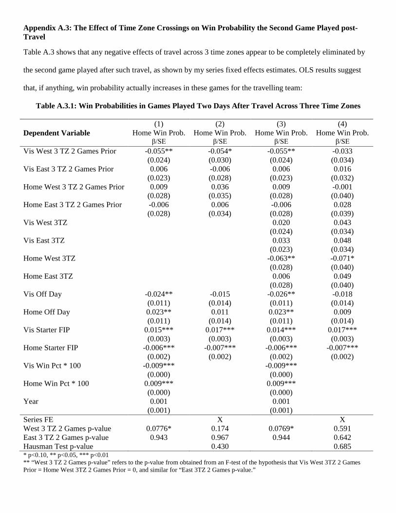
Appendix A.3: The Effect of Time Zone Crossings on Win Probability the Second Game Played post-Travel

Table A.3 shows that any negative effects of travel across 3 time zones appear to be completely eliminated by

the second game played after such travel, as shown by my series fixed effects estimates. OLS results suggest

that, if anything, win probability actually increases in these games for the travelling team:

Table A.3.1: Win Probabilities in Games Played Two Days After Travel Across Three Time Zones

(1) (2) (3) (4) Dependent Variable Home Win Prob. Home Win Prob. Home Win Prob. Home Win Prob. β/SE β/SE β/SE β/SE Vis West 3 TZ 2 Games Prior -0.055** -0.054* -0.055** -0.033 (0.024) (0.030) (0.024) (0.034) Vis East 3 TZ 2 Games Prior 0.006 -0.006 0.006 0.016 (0.023) (0.028) (0.023) (0.032) Home West 3 TZ 2 Games Prior 0.009 0.036 0.009 -0.001 (0.028) (0.035) (0.028) (0.040) Home East 3 TZ 2 Games Prior -0.006 0.006 -0.006 0.028 (0.028) (0.034) (0.028) (0.039) Vis West 3TZ 0.020 0.043 (0.024) (0.034) Vis East 3TZ 0.033 0.048 (0.023) (0.034) Home West 3TZ -0.063** -0.071* (0.028) (0.040) Home East 3TZ 0.006 0.049 (0.028) (0.040) Vis Off Day -0.024** -0.015 -0.026** -0.018 (0.011) (0.014) (0.011) (0.014) Home Off Day 0.023** 0.011 0.023** 0.009 (0.011) (0.014) (0.011) (0.014) Vis Starter FIP 0.015*** 0.017*** 0.014*** 0.017*** (0.003) (0.003) (0.003) (0.003) Home Starter FIP -0.006*** -0.007*** -0.006*** -0.007*** (0.002) (0.002) (0.002) (0.002) Vis Win Pct * 100 -0.009*** -0.009*** (0.000) (0.000) Home Win Pct * 100 0.009*** 0.009*** (0.000) (0.000) Year 0.001 0.001 (0.001) (0.001) Series FE West 3 TZ 2 Games p-value

0.0776*

X 0.174

0.0769*

X 0.591

East 3 TZ 2 Games p-value 0.943 0.967 0.944 0.642 Hausman Test p-value 0.430 0.685 * p<0.10, ** p<0.05, *** p<0.01 ** “West 3 TZ 2 Games p-value” refers to the p-value from obtained from an F-test of the hypothesis that Vis West 3TZ 2 Games Prior = Home West 3TZ 2 Games Prior = 0, and similar for “East 3TZ 2 Games p-value.”

Appendix A.4: Travel Effects in the First and Second Half of the Season and After the Amphetamine Ban

To test the theory that travel becomes more damaging to player performance as the season progresses and

players become more fatigued and susceptible to injury, I interact my three time zone crossing variables with an

indicator for the game being played in the second half of the season. Table A.4.1 shows that the null hypothesis

that travel has the same impact on win probability in both halves of the season cannot be rejected at even the

10% level. However, since the coefficients on these interaction terms are consistent with the hypothesis that

travel in the second half of the season is more detrimental, I expand my sample size to 1977-2013. Table A.4.2

shows that it is even more difficult to reject the null hypothesis that travel has the same effect on win

probabilities in both halves of the season when using data from 1977-2013. Table A.4.3 shows that the 2006

amphetamine ban in MLB had no effect on the relationship between travel and win probability.

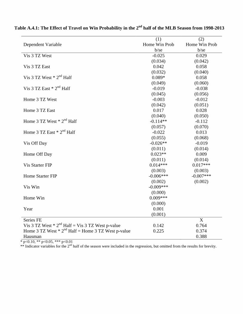
Table A.4.1: The Effect of Travel on Win Probability in the 2nd half of the MLB Season from 1998-2013

(1) (2) Dependent Variable Home Win Prob Home Win Prob b/se b/se Vis 3 TZ West -0.025 0.029 (0.034) (0.042) Vis 3 TZ East 0.042 0.058 (0.032) (0.040) Vis 3 TZ West * 2nd Half 0.089* 0.058 (0.049) (0.060) Vis 3 TZ East * 2nd Half -0.019 -0.038 (0.045) (0.056) Home 3 TZ West -0.003 -0.012 (0.042) (0.051) Home 3 TZ East 0.017 0.028 (0.040) (0.050) Home 3 TZ West * 2nd Half -0.114** -0.112 (0.057) (0.070) Home 3 TZ East * 2nd Half -0.022 0.013 (0.055) (0.068) Vis Off Day -0.026** -0.019 (0.011) (0.014) Home Off Day 0.023** 0.009 (0.011) (0.014) Vis Starter FIP 0.014*** 0.017*** (0.003) (0.003) Home Starter FIP -0.006*** -0.007*** (0.002) (0.002) Vis Win -0.009*** (0.000) Home Win 0.009*** (0.000) Year 0.001 (0.001) Series FE Vis 3 TZ West * 2nd Half = Vis 3 TZ West p-value

0.142

X 0.764

Home 3 TZ West * 2nd Half = Home 3 TZ West p-value 0.225 0.374 Hausman 0.388

* p<0.10, ** p<0.05, *** p<0.01 ** Indicator variables for the 2nd half of the season were included in the regression, but omitted from the results for brevity.

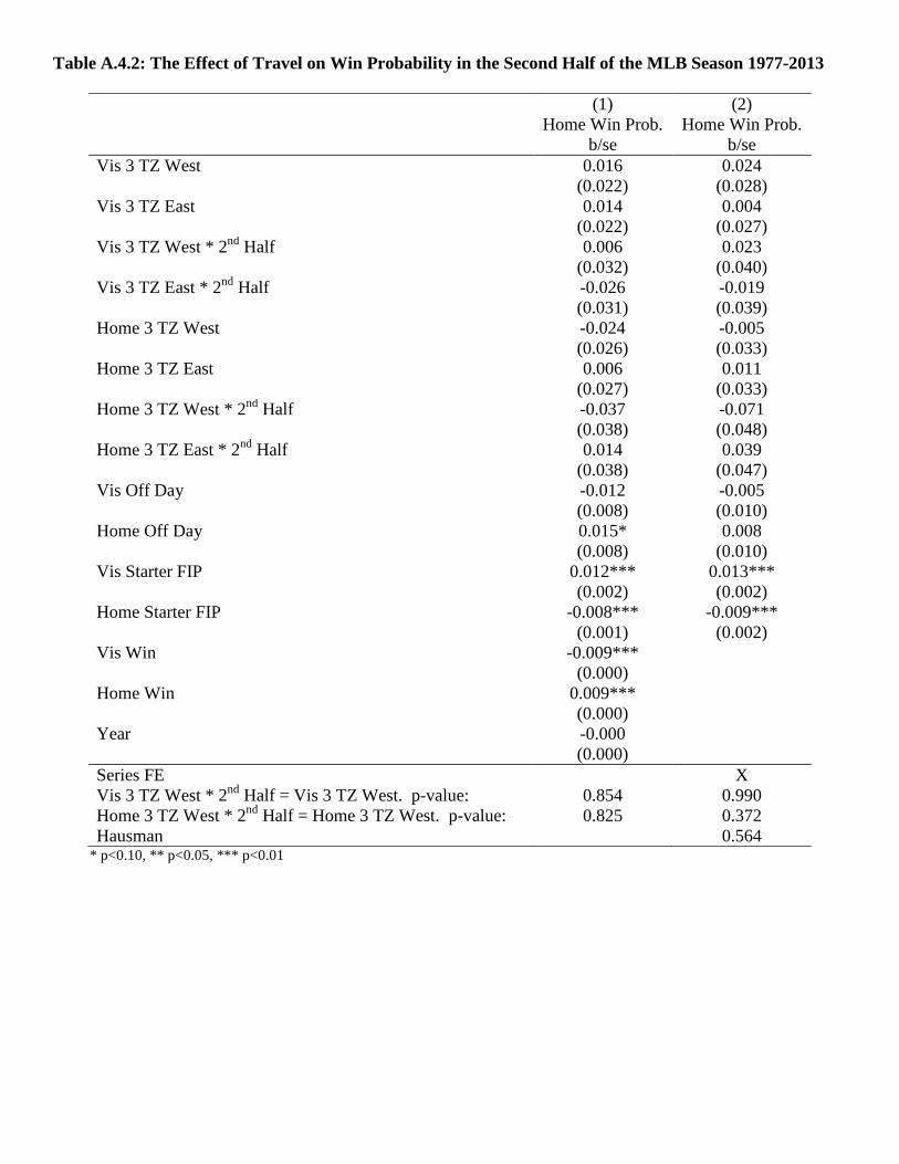
Table A.4.2: The Effect of Travel on Win Probability in the Second Half of the MLB Season 1977-2013

(1) (2) Home Win Prob. Home Win Prob. b/se b/se Vis 3 TZ West 0.016 0.024 (0.022) (0.028) Vis 3 TZ East 0.014 0.004 (0.022) (0.027) Vis 3 TZ West * 2nd Half 0.006 0.023 (0.032) (0.040) Vis 3 TZ East * 2nd Half -0.026 -0.019 (0.031) (0.039) Home 3 TZ West -0.024 -0.005 (0.026) (0.033) Home 3 TZ East 0.006 0.011 (0.027) (0.033) Home 3 TZ West * 2nd Half -0.037 -0.071 (0.038) (0.048) Home 3 TZ East * 2nd Half 0.014 0.039 (0.038) (0.047) Vis Off Day -0.012 -0.005 (0.008) (0.010) Home Off Day 0.015* 0.008 (0.008) (0.010) Vis Starter FIP 0.012*** 0.013*** (0.002) (0.002) Home Starter FIP -0.008*** -0.009*** (0.001) (0.002) Vis Win -0.009*** (0.000) Home Win 0.009*** (0.000) Year -0.000 (0.000) Series FE Vis 3 TZ West * 2nd Half = Vis 3 TZ West. p-value:

0.854

X 0.990

Home 3 TZ West * 2nd Half = Home 3 TZ West. p-value: 0.825 0.372 Hausman 0.564

* p<0.10, ** p<0.05, *** p<0.01

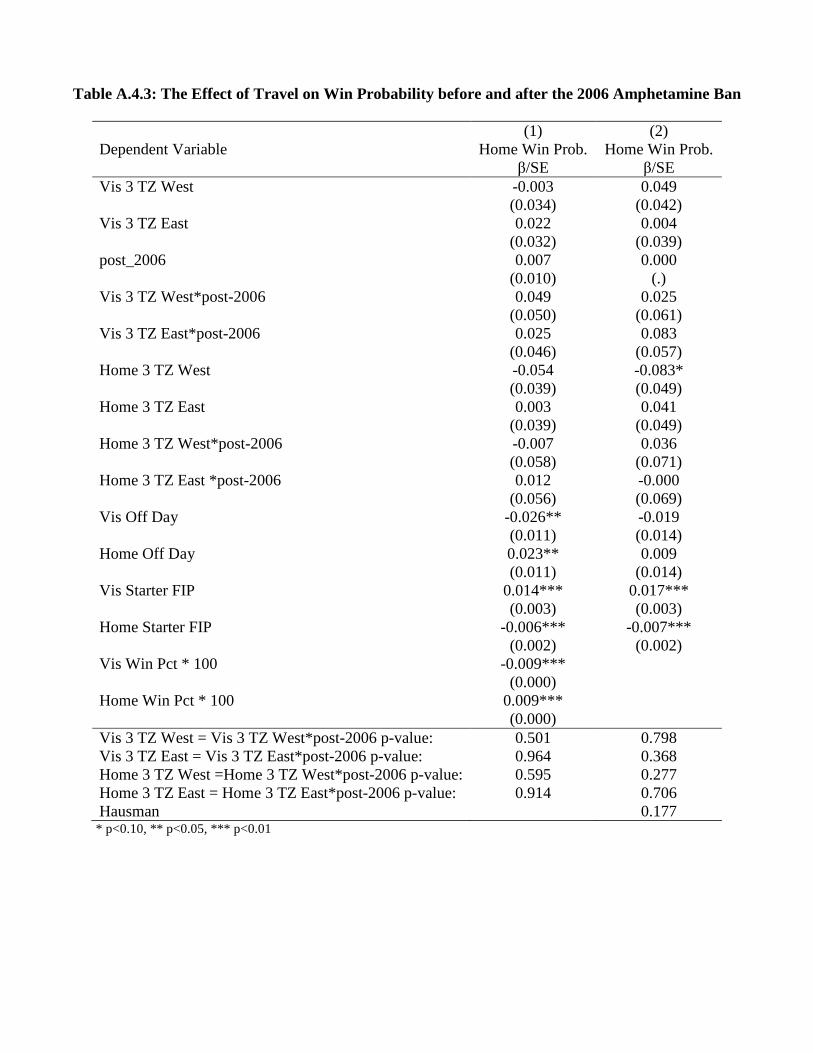
Table A.4.3: The Effect of Travel on Win Probability before and after the 2006 Amphetamine Ban

(1) (2) Dependent Variable Home Win Prob. Home Win Prob. β/SE β/SE Vis 3 TZ West -0.003 0.049 (0.034) (0.042) Vis 3 TZ East 0.022 0.004 (0.032) (0.039) post_2006 0.007 0.000 (0.010) (.) Vis 3 TZ West*post-2006 0.049 0.025 (0.050) (0.061) Vis 3 TZ East*post-2006 0.025 0.083 (0.046) (0.057) Home 3 TZ West -0.054 -0.083* (0.039) (0.049) Home 3 TZ East 0.003 0.041 (0.039) (0.049) Home 3 TZ West*post-2006 -0.007 0.036 (0.058) (0.071) Home 3 TZ East *post-2006 0.012 -0.000 (0.056) (0.069) Vis Off Day -0.026** -0.019 (0.011) (0.014) Home Off Day 0.023** 0.009 (0.011) (0.014) Vis Starter FIP 0.014*** 0.017*** (0.003) (0.003) Home Starter FIP -0.006*** -0.007*** (0.002) (0.002) Vis Win Pct * 100 -0.009*** (0.000) Home Win Pct * 100 0.009*** (0.000) Vis 3 TZ West = Vis 3 TZ West*post-2006 p-value: 0.501 0.798 Vis 3 TZ East = Vis 3 TZ East*post-2006 p-value: 0.964 0.368 Home 3 TZ West =Home 3 TZ West*post-2006 p-value: 0.595 0.277 Home 3 TZ East = Home 3 TZ East*post-2006 p-value: 0.914 0.706 Hausman 0.177

* p<0.10, ** p<0.05, *** p<0.01