Effect of world fertility scenarios on international livingstandards

Author

Guest, RS, McDonald, IM

Published

2004

Journal Title

The Economic Record

DOI

https://doi.org/10.1111/j.1475-4932.2004.00179.x

Copyright Statement

© 2004 Blackwell Publishing. This is the author-manuscript version of the paper. Reproduced inaccordance with the copyright policy of the publisher.

Downloaded from

http://hdl.handle.net/10072/5330

Link to published version

http://www.blackwellpublishing.com/

Griffith Research Online

https://research-repository.griffith.edu.au

13/08/2003

The Effect of World Fertility Scenarios on International Living Standards

Ross S. Guest Griffith University

Australia

Ian M. McDonald The University of Melbourne

Australia

ABSTRACT

This paper applies a two good, multi-region Ramsey-Solow model to determine the impact of future demographic change on international living standards and the optimal rate of national saving. Notable features of the model include: an outward looking model of utility, a premium in the interest rate for capital importing regions, an exchange rate expressed as the relative price of traded and non-traded goods, and a vintage model of production. The world economy is divided into nine regions consisting of the eight regions in the United Nations long run demographic projections (1998 Revision) plus Japan as a separate region. The model is simulated for the low, medium and high fertility scenarios as projected for all regions by the United Nations. The model suggests that there will be a flow of international capital from the ageing regions to the younger regions; and that the world interest rate will fall. The lower world interest rate will cause a loss in living standards for ageing regions, the lenders, and a gain for the younger regions, borrowers. Lower fertility leads to greater downward movement in the world interest rate, thereby increasing the loss to ageing regions and the gain to younger regions of demographic change. The impact on living standards of alternative fertility rates is dominated by the dependency effect, with the capital widening and capital intensity effects playing minor roles. The real exchange rate response to demographic change turns out to be small in this model, particularly for the developing regions.

1

The Effect of Fertility Rates on International Living Standards and Saving in a

World Model with Flexible Real Exchange Rates 1. Introduction There is currently, in OECD countries in particular, a vigorous debate about the

macroeconomic impact of future demographic change. Public concern is widespread

that future demographic change will imply lower living standards. This concern has led

to pressure on policy makers in high income countries to attempt by policy change to

increase the fertility rate. However, the theoretical and empirical evidence is

ambiguous. The transition to lower population growth caused by low fertility yields a

short term dividend for living standards in the form of lower youth dependency and

lower capital widening requirements. This dividend is offset later on by higher old age

dependency. For a discussion along with simulation results see Weil, 1999; Elmendorf

and Sheiner, 2000; and Guest and McDonald, 2002(c).

These models are, however, single region models. In a multi-region framework

the effect on living standards depends on the effects of lower fertility rates on net

international capital flows, through the effect on saving and investment flows, which in

turn alters world interest rates. The effect of changing world interest rates on living

standards differs for borrowing and lending regions. For borrowers the effect on

income is positive while for lenders it is negative. Also, different rates of population

ageing among regions will tend to alter real exchange rates which can in turn impact

on relative living standards. Rapidly ageing regions, for example, will tend to

experience appreciating real exchange rates to the extent that the increase in the

relative price of labour in these countries tends to increase the price of non-traded

relative to traded goods since non-traded goods are more labour intensive.

2

This paper quantifies, by simulation, the impact of three scenarios of future

demographic change, based on alternative fertility rates, on world interest rates and

living standards. The three different fertility assumptions – low, medium and high –

implied by UN population projections for the 21st century are used.

There are several classes of multi-regional macroeconomic models that can be

used to simulate the macroeconomic implications of demographic change. The model

in this paper is a two good, multi-regional Cass-Ramsey-Solow model. Although

generations are not overlapping in this framework, heterogeneity of workers and

consumers is captured by weighting for age-specific productivity and consumption

needs, respectively. Single good versions of this class of models are the OECD model

in Borsch-Supan (1996) and the two region open economy model in Cutler et al.

(1990). A variation on this approach is the overlapping generations models of Turner

et al. (1998) using the OECD’s Minilink model, the models of the Ingenue Team

(2001) and Fougere, M. and Merette, M. (1999), and the macroeconometric model of

Masson and Tryon (1990). The distinction that we make here between traded and non-

traded goods puts this model in the class of the multi-good, multi-region, general

equilibrium models such as the G-cubed model (see, for example, McKibbin, W.J. and

Nguyen, J., 2001), although the model here has less complexity than, for example, the

G-cubed model.

2. Demographic projections

In this model, the world economy is divided into nine regions consisting of the eight

regions in the United Nations (2000) long run demographic projections plus Japan as a

separate region. The nine regions are: Africa, Asia (excluding China, India and Japan),

China, Europe, India, Japan, Latin America, North America and Oceania. This is a

3

larger number of regions than has been adopted in other models listed above. We

choose for comparison the low, medium and high fertility scenarios in the United

Nations projections (up to 2150). The medium scenario assumes that fertility in all

major areas stabilizes at replacement level around 2050; the low scenario assumes that

fertility is half a child lower than in the medium scenario; and the high scenario

assumes that fertility is half a child higher than in the medium scenario.

For each of these population scenarios, employment projections by age and sex

are calculated from the International Labour Organisation (ILO, 2001) database: Key

Indicators of the Labour Market (KILM). These data provide labour force and

population by age group and sex for each country in the world for the latest year –

typically 1999 or 2000. From these data the aggregate labour force participation rates

(LFPR) for each of the nine regions, by age group, are calculated. These age and sex-

specific LFPRs are assumed to be the age-specific employment to population (L/N)

ratios.

There is quite a wide variation in the L/N ratios between regions. For example,

for males and females combined the L/N for 15-24 year olds for Europe is 0.47 while it

is 0.79 for China and 0.66 for North America. We assume that it is unlikely that such

divergences will persist as economic development progresses. Hence employment

projections for each region are calculated by assuming that the age-specific L/N ratios

(for both sexes) partially converge toward those of North America according to the

following formula:

( ) ( ) ( )( )

σ

=

−−

aj

NAa

ajaj NLNL

NLNL,1

,1, (1)

where j is the year from 2001 to 2150, NA is North America, a is the age group, σ is

the convergence parameter set equal to 0.025.

4

Following Cutler et al. (1990) and Elmendorf and Sheiner (2000) the

employment and population numbers are weighted to account for, respectively, age-

specific differences in labour productivity and consumption needs. Labour productivity

of middle-aged workers is higher than that of both younger and older workers and this

is reflected in their relative wages. In the absence of reliable data for all regions on

labour productivity by age, we adopt as an expediency the age-productivity relation in

Miles (1999), where the productivity weight is a quadratic function of age: 0.05age –

0.0006age2. Consumption needs also vary by age – in particular, education and

medical expenses. To allow for this, we apply the consumption weights in Cutler et al

(1990); that is 0.72 for 0-19 year olds, 1.0 for 20-64 year olds and 1.27 for over 64

year olds. Both productivity weights and consumption weights are non-gender specific.

The aggregate weighted L/N ratio for each region is the support ratio (Cutler et

al., 1990). A decrease in the support ratio implies a diminished capacity to meet a

given level of consumption needs per capita. An increase in the support ratio implies

the opposite. Chart 1 plots the support ratios for the nine regions for the medium

fertility scenario which we refer to as the base case. The five regions with imminently

declining support ratios are Japan, Europe, China, North America and Oceania.1 These

regions will be referred to here as the ageing regions. The other four regions: Africa,

Asia, India and Latin America, are younger in that their support ratios follow a hump-

shape, rising initially then declining. These regions will be described as the younger

regions. This classification of regions is also valid for the low fertility and high fertility

scenarios.

In order to ensure that the economy converges to a new steady state, the

demographic projections described above are applied only for the period 2000 to 2100,

5

at which point the rate of growth of aggregate weighted employment is assumed to

remain constant. This constant growth rate is also the rate at which aggregate weighted

population is assumed to grow indefinitely.

3. The model

The important features of the model are described here. A full list of equations and

variables are given in the Appendix. The method of solving the model is also described

in the Appendix.

3.1 Firms

Output of traded and non-traded goods is produced according to vintage, Cobb-

Douglas technology with constant returns to scale. While the vintage capital model,

appropriately calibrated, yields the same long run solution as the homogeneous capital

model (Solow, 1960), there can be differences in the short run response to shocks of,

for example, a demographic nature (Guest and McDonald, 2001). For a generic

comparison of vintage and homogenous capital models see Greenwood (1977). One

practical reason for adopting a vintage rather than homogeneous capital model is that it

obviates the need for adjustment costs in investment.

As in the two good model in Obstfeld and Rogoff, 1996, it is assumed that non-

traded (N) goods cannot be capital goods, only consumer goods, which implies that the

output of N goods is equal to the consumption of N goods. There are two reasons for

this assumption: it simplifies the solution procedure (see Appendix) and it captures, to

an approximation, the observation that consumption goods and services have a higher

non-traded component than do traded goods.

3.2 Consumers

1 The decline in the support ratio for Europe and for China does not commence until 2010 and 2005,

6

Each region is populated by infinitely lived dynasties of people who differ only in that

their consumption demands are age-specific. We consider the behaviour of a

representative consumer whose age is the average age of the population, weighted by

the population shares of each age group. For this consumer, we adopt the model of

consumption in Obstfeld and Rogoff (1996), modified for a reference level of

consumption in the intertemporal utility function (discussed below).

In this model, the consumer is faced with both an intratemporal and an

intertemporal maximisation problem. The intratemporal optimisation problem is

solved by optimally allocating a given value of consumption, measured as an index,

between traded and non-traded goods. It is assumed that while all consumers are

intratemporal optimisers not all consumers are intertemporal optimisers. Rather 30%

of consumers are rule-of-thumb consumers, meaning that they always consume a fixed

proportion of their income. This is a common assumption in applied economy-wide

models; in the context of population ageing see, for example, the application of the

MSG3 model in McKibbin and Nguyen, 2001 and the OECD’s MINILINK model in

Turner et a., 1998.

The consumers who optimise intertemporally maximise an outward-looking

utility function, as in Carroll et al. (1997), where each consumer compares their

consumption against the consumption of others in deriving their utility. Carroll et al.

(1997) cite a range of evidence from the literature, both theoretical and empirical, in

support of two alternative forms of what they call “comparison utility”.2 From our

point of view, perhaps the most compelling argument is that models of comparison

respectively. However, the initial rise in the support ratio is very small. 2 One form of comparison utility is the “outward-looking” model that we adopt here. The other form is the “inward-looking” model in which consumers compare their consumption with their own past consumption rather than the consumption of others. Both forms of comparison utility generate a type of habit formation in consumption which implies the sort of persistence in consumption that we observe in

7

utility generate persistence in the time series of consumption that matches the

persistence found in the actual data.

3.3 Assumptions about capital mobility and productivity growth

We assume that capital is not perfectly mobile which is consistent with extensive

evidence. For a discussion of the various explanations of imperfect capital mobility see

Gordon and Bovenberg (1996); and for a survey of the evidence on the Feldstein-

Horioka puzzle as an indicator of imperfect capital mobility see Coakley, Kulasi and

Smith (1999). The most important explanation according to Gordon and Bovenberg

(1996) is asymmetric information between investors of different countries. In

particular, foreign investors know less about the economic prospects of another

country than do the residents of that country. Gordon and Bovenberg develop a

theoretical model, for which they find empirical support, in which the interest rate, r, in

capital importing countries is higher than the world interest rate, r . The latter is the

rate received by lenders in capital exporting countries. The interest rate premium in

capital importing countries is a function of the amount of capital imported. There is

also evidence that countries – small countries in particular - face a risk premium that

depends on their existing stock of foreign debt (see Juttner and Luedecke (1991) for

the case of Australia). We allow for both of these mechanisms – asymmetric

information and a risk premium – in determining the interest rate.

Steady state labour productivity growth is exogenous and constant at 1.5% per

annum for all regions. This implies two things – first, that there is no influence of

demographic change on technical progress and, second, that there is no convergence of

labour productivity among the nine regions. On the effect of demographic change on

technical progress both the theoretical and empirical evidence is ambiguous, as

the data. This is the main motivation for adopting comparison utility in this paper and from that point of

8

discussed by Cutler et al. (1990, p. 38). Consider slower population growth. On the

one hand slower population growth makes innovation less profitable by reducing the

gains from economies of scale through the spreading of fixed costs; and a smaller

youth share of the population may reduce innovation through a loss of “dynamism”;

also, in endogenous growth models such as that in Steinman et al. (1998) lower

population growth results in less human capital accumulation and therefore a lower

growth rate of labour productivity. On the other hand, there are several potential

mechanisms through which slower population growth can boost labour productivity.

Less urban congestion, for example, could enhance labour productivity growth. Also,

slower labour force growth implies a higher relative price of labour and therefore

greater incentive to innovate through capital investment. And the model in Fougere

and Merrete (1998) shows that slower population growth will increase human capital

formation, through tax effects, which could boost productivity growth if endogenous

growth occurs through human capital formation. The empirical evidence on the effect

of fertility on labour productivity is relatively scarce - see for example Galor et al.

(1997), Ahituv (2001) and Hondroyiannis and Papapetrou (1999) - and somewhat

conflicting. Hence the assumption here of zero net effect of demographic change on

total factor productivity growth seems to be a reasonable starting point.

With respect to the zero convergence assumption, Barro and Salai-Martin

(1995, p.26) report that the hypothesis of absolute convergence – where poor countries

catch-up with rich countries in their GDP per capita, without allowing for any control

variables – has received mixed empirical support.3 Nevertheless, most multi-regional

macroeconomic models adopt some form of productivity convergence. Using the

view it does not matter whether we adopt the outward-looking model or the inward-looking model. 3 The hypothesis of conditional convergence, which controls for various characteristics of economies, has received stronger empirical support. However, even the testing of this weaker hypothesis faces some

9

OECDs multi-regional “Minilink” model, Turner et al (1998) assume slow

convergence in the rates of technical progress of their five world regions, as distinct

from convergence in their productivity levels. The Ingenue Team (2001) assume

extremely slow convergence in levels of productivity – the gap between rich and poor

countries appears to close by about 20% over 100 years. Dynamic intertemporal

general equilibrium models, such as the G-Cubed Model, also typically incorporate

some form of technology catch-up (McKibbin, 1999). In this paper, zero convergence

in total factor productivity is assumed because, in our initial simulations, we found that

all but a very small rate of convergence tended to swamp the effects of differences in

fertility rates that we were attempting to isolate. As a result of this, and the uncertainty

in the empirical literature about productivity convergence, we felt that zero

convergence was a reasonable assumption for our purposes.

4. The simulation method

The solution procedure is to first calibrate an initial steady state which implies that

both population and employment are initially growing at constant rates. The

demographic projections are then introduced as unanticipated “shocks”. Cutler et al.

(1990) argue that “it is not obvious how best to model [demographic change] as a

single shock” (p.23). The approach they and others typically adopt is to assume that

the population has been stable at which point a demographic shock occurs so that

employment and population follow the projections described above. Following the

shock, it is assumed that consumers and firms know the future demographic structure

and choose optimal consumption and investment levels accordingly.

serious econometric problems. See Durlauf and Quah in Taylor and Woodford eds. (1999) for a comprehensive discussion of the theory and empirical tests of convergence hypotheses.

10

Once the initial steady state is defined for each region, the optimal path in

response to the demographic shock is determined by finding the new initial value of

the consumption index that leads to the steady state. Given the resulting paths for all

nine regions of the world, the model is closed by ensuring that the world current

account balance is zero. This is achieved by an iterative process as follows. An

arbitrary initial path of the world interest rate is chosen over a very long horizon and,

given this path, the optimal plan for each region is calculated so that the economy

reaches a steady state. Then a new path of the world interest rate is chosen by adjusting

the interest rate in each year in which the world current account balance is not equal to

zero. This process is repeated until the world current account balance is equal to zero

in each year.

5. Saving, investment, net capital flows and the world rate of interest

Figure 2 shows the impact of the future patterns of demographic change on the world

rate of interest. Under all fertility scenarios the world interest rate falls, following a

small adjustment upwards immediately following the shock.

The demographic shock initially increases optimal saving slightly in the ageing

regions (as identified in Figure 1) because their consumption possibilities are lower as

a result of ageing. It is therefore optimal to smooth consumption by making an

immediate downward adjustment to consumption starting from a steady state.4 After a

brief initial period, saving steadily declines for the ageing regions, reflecting their

declining capital requirements which is evident in the investment series in Figure 3.

The younger regions initially reduce optimal saving because their consumption

possibilities are higher as a result of their populations initially becoming younger for a

11

period of some years, as indicated by their rising support ratios. After this initial

adjustment saving rises for these regions, reflecting their growing capital requirements.

The net effect of these saving and investment patterns is a small initial increase

in the world interest rate following the ageing shock followed by a decline by about

one percentage point from maximum to minimum. For base case demographics the

world interest rate remains below its current level from 2010 onwards.

For most of the next century – from 2020 onwards - the lower are fertility rates

around the world the lower is the world interest rate (Figure 2). A lower fertility

scenario amounts to a bigger ageing shock which magnifies the response of world

saving and investment, resulting in a larger initial rise and larger subsequent fall in the

world interest rate. A higher world fertility scenario has converse effects – a smaller

demographic shock resulting in a smaller fall in the world interest rate.

Alternative world fertility scenarios have different effects on savings of ageing

regions compared with younger regions. For illustration, Figure 3 compares the effect

of the demographic shock caused by the medium (base) and low fertility scenarios on

saving, investment and the current account balance. For the younger regions, the effect

of low fertility on saving is muted compared with the effect on ageing regions. The

reason for this can be seen by considering the income and substitution effects of a

lower interest rate. For ageing regions, who are lenders, lower interest rates reduce

saving through substitution and through income. But younger regions are debtors,

borrowing to finance their higher consumption possibilities. For debtors, lower interest

rates have offsetting income and substitution effects on saving. The substitution effect

tends to reduce saving while the income effect tends to increase it. The net result is a

small decrease in saving relative to that for ageing regions.

4 Note that in a model with imperfect capital mobility it is not optimal to adjust immediately to the new

12

Current account surpluses of the ageing regions are matched by current account

deficits of the younger regions, implying the export of capital from the former to the

latter.5 Lower fertility rates impact only very slightly on the size of these capital flows

– saving is lower but so is investment.

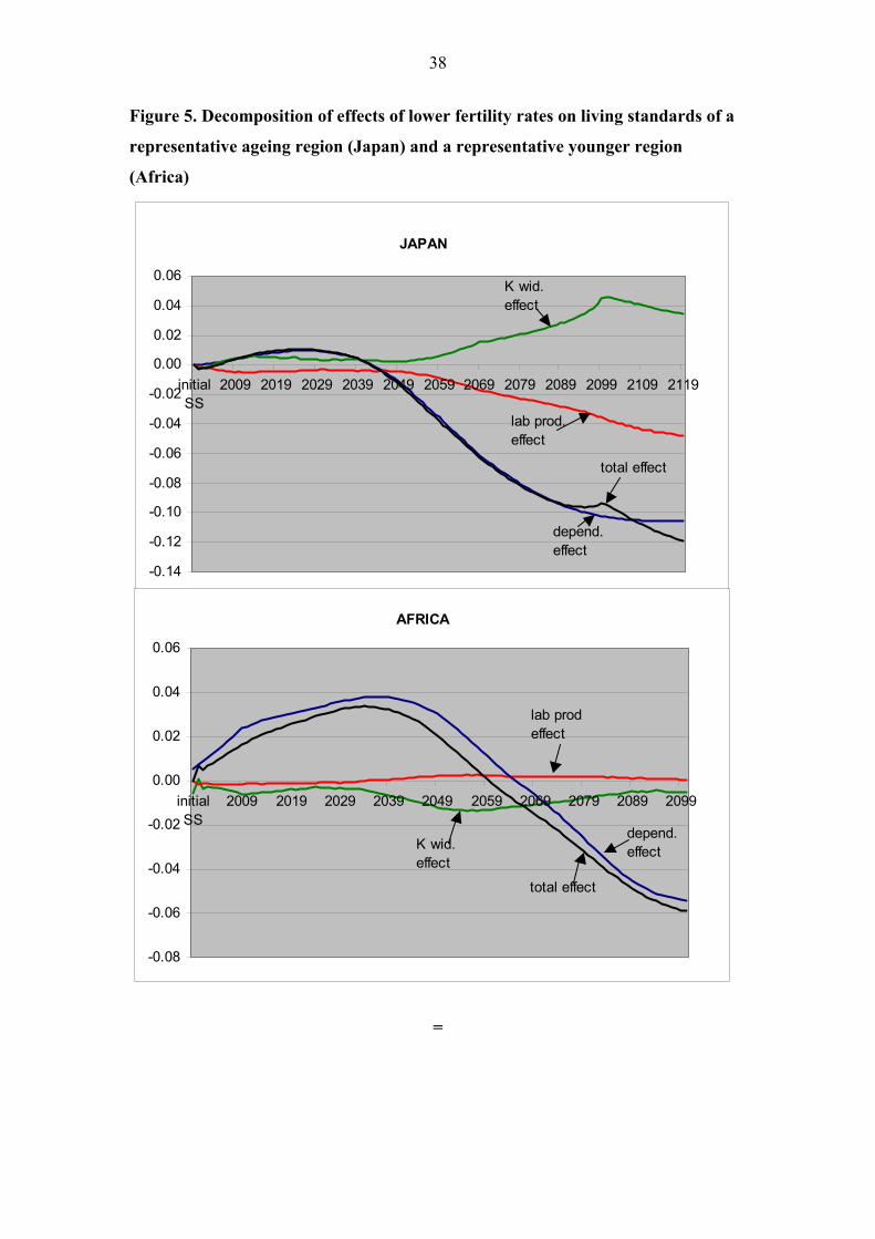
6. Living standards

Living standards are defined as aggregate consumption per equivalent person, C/P.

The impact on living standards of a demographic shock is the net result of three

effects: the dependency effect, the capital widening effect and a labour productivity

effect, see Elmendorf and Sheiner (2000)6.

Higher (lower) overall dependency (the combination of youth and old age

dependency) implies fewer (more) workers per person, which reduces (increases)

consumption possibilities. The capital widening effect refers to the impact of a change

in the rate of growth of employment on the level of investment needed to maintain a

given capital-labour ratio. Lower (higher) employment growth increases (decreases)

consumption possibilities. The labour productivity effect refers to the temporary

change in labour productivity resulting from the temporary change in capital labour

ratios as a result of a demographic shock. In a two good model such as this, average

labour productivity is also affected by shifting of labour between sectors of unequal

labour productivity. Since the T sector in this model has higher labour productivity

than the N sector, any relative expansion or contraction of the T sector has an

steady state level of consumption because the interest rate varies along the optimal path and this alters the path of consumption. 5 The description of ageing regions as creditors and younger regions as debtors refers to the short term response to the ageing shock, typically for the first two decades at least. Beyond that, the pattern is reversed in some cases. Also, Europe is neither a significant creditor or large debtor in the short term. This is consistent with the pattern of its support ratio (Figure 1) which shows a small rise initially before it declines. 6 Elmendorf and Sheiner refer to a capital intensity effect which we call a labour productivity effect because it is perhaps more descriptive for this model (see discussion below).

13

expansionary or contractionary effect on average labour productivity.7 The assumption

here that N sector output consists entirely of consumption goods - that is, YN = CN -

means that any adjustment to the aggregate consumption to output ratio must fall on

the T sector. In the case of Japan for example, the aggregate consumption to output

ratio rises following the shock and this draws labour from the higher productivity T

sector to the low productivity N sector. Hence average labour productivity falls. For

Africa however, the process works in reverse; the aggregate consumption to output

ratio falls therefore labour is released into the T sector which raises average labour

productivity. The implication is that the low fertility scenario results in a bigger fall in

average labour productivity than does the base scenario for ageing regions like Japan;

and a bigger rise in average labour productivity than under the base case for younger

regions like Africa.

Figure 4a illustrates the effects of the demographic shock on living standards

for both a representative ageing/creditor region (Japan) and a representative

younger/debtor region (Africa) under base, low and high fertility scenarios.8 It can be

seen that the demographic shock has different impacts on living standards for the

ageing regions compared with the younger regions. The shock reduces living standards

in the ageing regions and raises living standards in the younger regions. This is due to

two effects. First, because ageing regions face an imminent decline in their support

ratios (Figure 1) their living standards fall, relative to the no demographic change

outcome. Younger regions, however, face rising support ratios for an initial period

(Figure 1). This allows them to enjoy living standards that are higher than they would

be if there were no demographic change. Second, the reduction in the world rate of

7 The strong assumption: YN=CN is not necessary for this a result to apply. It only requires that (C/Y)N>(C/Y)T and that (K/L)T>(K/L)N.

14

interest reduces incomes in the ageing regions because they are creditors and increases

income in the younger regions, who are debtors. These effects of the demographic

shock – higher living standards for ageing regions and lower living standards for

younger regions – apply for all fertility scenarios.

A lower fertility shock tends to improve living standards in the near term and

reduce them later on (see Figures 4a and 4b). Lower fertility has offsetting effects on

consumption possibilities. There are consumption dividends from lower youth

dependency and lower capital widening requirements which are offset by higher old

age dependency later on. How the net effect of these is smoothed out depends on the

path of the interest rate. Lower fertility rates put downward pressure on interest rates.

This creates an intertemporal substitution effect, which is to bring consumption

forward. The result is the pattern in Figure 4b showing higher consumption for an

initial period under lower fertility, but lower consumption later on.

Figures 4a and 4b show only two regions in order to clearly illustrate the

patterns in graphical form. For all regions, the effects of lower and higher fertility

relative to medium fertility are summarised in Table 2. As can be seen from this table,

it is generally the case that the initial gain from lower fertility is smaller for the ageing

regions, and is more short-lived, than for the younger regions. The reason is the

different income effects, for ageing/lending regions and younger/borrowing regions, of

the change in interest rates brought by lower fertility.

8 Japan and Africa are extreme examples of ageing and younger regions, respectively. They are chosen to emphasise the contrast between these two types of regions. They are representative in that the other regions in their group are similar to them.

15

LOW FERTILITY

Nth Am Jap China Europe Oceania India Latin Am Africa Asia2010 1.3 0.5 1.6 1.0 1.8 2.3 2.1 1.7 2.22020 1.6 1.0 2.2 1.4 2.2 3.2 2.8 2.6 2.82030 0.9 1.0 1.7 1.1 1.6 2.9 2.6 3.3 2.72040 -0.6 0.3 0.4 0.0 0.3 1.8 1.5 3.1 1.82050 -2.9 -1.5 -1.8 -2.1 -1.9 -0.7 -0.8 1.8 -0.32100 -14.8 -9.7 -7.8 -10.8 -7.8 -7.7 -7.2 -5.9 -7.0

*The above panel shows that, at any given time, ageing regions generally face smaller gains and/or bigger losses from low fertility than do younger regions

HIGH FERTILITY

Nth Am Jap China Europe Oceania India Latin Am Africa Asia2010 -1.8 -0.6 -1.1 -1.6 -0.8 -2.2 -2.2 -1.7 -2.02020 -1.9 -1.0 -1.8 -1.7 -1.0 -3.0 -2.7 -2.5 -2.72030 -1.0 -0.9 -1.6 -1.0 -0.9 -2.8 -2.5 -2.9 -2.62040 -0.1 -0.4 -0.9 0.5 -1.1 -2.2 -1.9 -2.9 -2.12050 1.1 1.1 0.3 2.6 -0.9 -0.9 -0.5 -2.4 -0.92100 7.2 5.2 3.8 5.3 2.8 3.4 3.4 2.4 3.4

*The above panel shows that, at any given time, ageing regions generally face bigger gains and/or smaller losses from high fertility than do younger regions

ageing regions younger regions

ageing regions

% change in consumption per equivalent person relative to medium fertility*

Table 2 Effects of low and high fertility on living standards

% change in consumption per equivalent person relative to medium fertility*younger regions

We now decompose the total effect on living standards into the three

component effects according to the following identity:

PL

LY

YC

PC=

which in per person or per worker units is

αα

yy

cc = (2)

We focus on the case of lower fertility for illustration – the results for higher

fertility are the converse of those for lower fertility. The dependency effect of lower

fertility describes the lower consumption possibilities that result from there being

fewer workers relative to consumers, which is the case once the short term reduction in

youth dependency is offset by the rise in old age dependency. The dependency effect is

the effect on consumption possibilities of a lower value of L/P = α and is therefore

approximated9 by, according to (2), ( ) [ ]baselowbasec ααα − . This gives the net effect of

a reduction in youth dependency and an increase in old age dependency. The capital

16

widening effect refers to the lower capital requirements of a more slowly growing

labour force, which increases consumption possibilities. A lower investment share of

output allows a higher consumption share (C/Y), other things equal. Therefore, the

capital widening effect is given by ( ) ( ) ( )[ ]baselowbase ycycy )()( ααα − . The labour

productivity effect refers to changes in Y/L=y holding all else constant and is given by

( ) [ ]baselowbase yyyc − .

The three effects of lower world fertility rates are plotted in Figure 5 for the

representative ageing region (Japan) and the representative younger region (Africa).

The dependency effect accounts for virtually the entire effect on living standards, with

the capital widening effect and labour productivity effects almost cancelling each other

out.

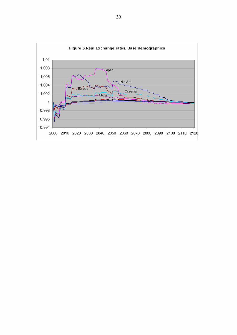
7. The role of the real exchange rate

The distinction between traded and non-traded goods adds quite a degree of

complexity to the model. The motivation for this was the possibility that different rates

of population ageing would alter the relative price of non-traded goods across regions.

The idea is that shortages of labour require imply higher real wages relative to the cost

of capital, which increases the relative prices of non-traded goods since they are

relatively labour intensive. Hence the rapidly ageing regions would face higher relative

prices of non-traded goods and therefore higher real exchange rates, which could in

turn impact on living standards. Simulations revealed however that the real exchange

rate response to demographic shifts is quite small, especially for the developing

regions. See Figure 6.

9 Ignoring second order terms.

17

The exchange rate is determined by the interest rate which does not respond

much to the demographic changes simulated here. The maximum change in the interest

rate from peak to trough is about one percentage point. One reason for the modest

response of the interest rate is the equilibrating forces that operate when interest rates

change. Consider younger regions (Africa, Latin America and Asia) for whom

population ageing is relatively distant. They face strong demand for capital relative to

saving and therefore their foreign debt rises which raises their interest rates and hence

lowers the relative price of labour. (At the same time their relative abundance of labour

increases which further lowers the relative price of labour.) The higher return to saving

induces higher optimal saving and lower demand for capital which offsets the first

round effect on debt and interest rates. The reverse applies for regions facing current or

imminent population ageing. They face weak demand for capital relative to saving

which reduces their foreign liabilities and hence lowers their interest rates and hence

raises their relative price of labour. They face further pressure on the relative price of

labour from the shortage of working age people. The resulting fall in interest rates

encourages current consumption rather than saving which helps to reverse the process

of falling interest rates. These equilibrating effects mitigate the interest rate response to

demographic change.

The magnitude of the response of the real exchange rate also depends on the

difference in capital labour ratios between the two sectors (see Appendix B for

derivation). In general, the size of the gap between the capital labour ratios for the

traded and non-traded sectors determines the magnitude of the effect of a given

demographic change on the real exchange rate. Hence if there is very little difference

in the capital labour ratios then a proportional change in aggregate employment (via a

demographic shock) will cause very little proportional change in the exchange rate.

18

This is what happens for developing regions, especially Africa, India and Latin

America. They have very low overall capital labour ratios which means that the

absolute difference in those ratios for the two sectors is small. Hence the real exchange

rate response to demographic change is smaller for those regions. This effect, together

with the small response in the interest rate described above, means that the absolute

impact on the exchange rate is particularly small for developing regions.

8. Conclusion

From the simulations in this paper, four major conclusions stand out. First, under all

three of the UN demographic scenarios - that is, low, medium and high fertility, the

ageing regions will tend to be lenders and the young regions will tend to borrow. This

pattern reflects the greater investment opportunities in the younger regions, due to

faster employment growth. These investment opportunities will attract international

capital flows. Second, under all demographic scenarios world interest rates can be

expected to be lower for most of the next century. This is because, over this period,

demographic change will cause greater downward pressure on world investment than

on world saving. Third, demographic change, under all fertility scenarios, will have an

adverse effect on living standards in the ageing regions and a beneficial effect in the

young regions. The increased dependency in the ageing regions contrasted with a

period of decreased dependency in the younger regions is one reason for this. However

there is a second reason. Because ageing regions are lenders and therefore creditors,

lower interest rates will cause a loss in income and thus living standards. For young

regions, which are the borrowers and therefore debtors, low interest rates will improve

income and living standards. Fourth, the real exchange rate responses to the

demographic changes simulated here are relatively small and therefore will not play a

19

significant role in the effect on living standards. This is particularly so for the

developing countries because their capital labour ratios are lower than those of the

developed regions.

20

Appendix A This Appendix describes the analytics of the model and the solution procedure.

Let YT and YN be output of traded (T) and non-tradable (N) goods, respectively.

Let VT and VN be the number of vintages of capital employed in producing tradable and

non-tradable goods, respectively10. Assume that output is produced according to a

vintage production function with Cobb-Douglas technology:

( ) ( ) ([[ ]∑−

=

−−−−−−

− +−=1

0

1,1,,,

1, 1

TV

kTktTktTktTktT

kTtT lLIAδY γγ

δ )]

)]

)

)

(A1)

( ) ( ) ([[ ]∑−

=

−−−−−−

− +−=1

0

1,1,,,

1, 1

NV

kNktNktNktNktN

kNtN lLIAδY γγ

δ (A2)

which can be approximated by

( ) ( )( γγ δδ −−− ++−= 1

1,1, 1 TTTTTTTT lLIAYY (A3)

( ) ( )( γγ δδ −−− ++−= 1

1,1, 1 NNNNNNNN lLIAYY (A4)

which, in turn, can be expressed in intensive form where y is output in efficiency units

per equivalent worker.

( )( )

γγ δδ −

−

++

++−

=1

1, 111

TT

TTT l

lix

yy (A5)

( )( )

γγ δδ −

−

++

++−

=1

1, 111

NN

NNN l

lix

yy (A6)

Let qT and qN be the effective labour available to work on new capital. It can be shown

that for the T and N sectors ( )

δ++

=l

li 1q . To see this, note that

ALIi = and therefore

10 We follow the assumption in Obstfeld and Rogoff (1996) that only tradable goods can be transformed into capital. They describe this assumption as “inessential but helpful” (p.204). In our version of their model this assumption allows an analytic solution for lN and lT; otherwise numerical methods would be required.

21

( ) ( )11 )1(

11−−

=+

+=+

ALI

lALlIli . Therefore ( )

( )δδ ++

=+

=− l

lilALI 1

1

q is the ratio of new

capital, I, to effective labour available to work on new capital, ( )δ+− l1AL . The latter

consists of the share, l, of the increase in aggregate employment and the share, δ, of

aggregate employment that has been from capital that has been scrapped.

Investment in each of the two sectors is determined by the condition that the

marginal product of capital is equal to the user cost of capital, r+δ. Therefore

γ

δγ −

+

=1

1

TT r

q (A7)

γ

δγ −

+

=1

1

NN r

eq (A8)

The real wage, w, is equal to the marginal product of labour in each sector. That is,

( )( ) wqA TT =−− γγ γ111

(A9)

( )( ) wqAe NN =

−− γγ γ11

1 (A10)

The four equations (A7) to (A10) can be solved for the four endogenous

variables qT, qN, w and e. However, in order to determine iT and iN from qT and qN it is

necessary to allocate the exogenously given growth in aggregate employment between

lT and lN. This is done by first assuming that N goods cannot be capital goods, only

consumer goods. This implies that the output of N goods is equal to the consumption

of N goods (following the assumption in Obstfeld and Rogoff, 1996). To explain how

this allows us to separate out lT and lN we begin by describing the model of

consumption.

The consumer’s intratemporal maximization problem.

22

Define an index of total consumption for the representative consumer (see Table 1 for

the full list of variables) at time t:

( )11

,11

,1

1−−−

−+=

ψψ

ψψ

ψψψ

ψ µµ tNttTtt ccc (A11)

µt is time varying because the representative consumer’s relative preferences for traded

and non-traded goods vary with age. This reflects the observation that preferences for

medical and health services, which are essentially non-traded goods, are age-

dependent. In particular, we would expect that dependents, who are predominantly the

young and old, have a higher demand for non-traded relative to tradable goods than do

working age people. A simple way to accommodate this is to assume that age-based

variation in consumption demands reflects entirely variation in demand for non-

tradable relative to tradable goods. This implies that µ for the representative consumer

varies over time in proportion to variation in average consumption demands, defined

astP

N

. Therefore,

tt P

N

= 0µµ .

Total expenditure on cT and cN, measured in units of T goods is, dropping time

subscripts

NT eccE +≡ (A12)

In each period the consumer maximizes (A11) subject to (A12) yielding

( )ψ

µµ −=−

ec

c

T

N

1 (A13)

Combining (11) and (12) yields

( ) ψµµµ

−−+= 11 e

EcT ; and ( )( ) ψ

ψ

µµµ

−

−

−+−

= 111

eEpcN (A14)

Let PC be the price, in T goods, of a unit of the consumption index and it is defined as

the minimum E such that c=1. Using this and substituting (A14) into (A12) yields

23

( )[ ] ψψµµ −−−+= 1111 ePC (A15)

Given (A14), (A15) and the definition that E=cPC, gives

cP

c CT

ψ

µ−

=

1 ; and ( ) cPec CN

ψ

µ−

−= 1 (A16)

This solves the intratemporal maximization problem for the representative consumer.

The consumer’s intertemporal maximization problem.

It is assumed that a proportion, (1-ξ), of consumers are intertemporal optimisers and ξ

are rule-of-thumb consumers who consume a constant proportion of their income.

The utility that consumers derive from a given amount of consumption differs

according to their consumption demands. The representative consumer maximizes the

following intertemporal utility function:

( )βθ

β

ω −+

=

−−

∞

=∑ 1

1 11

1

t

tt

opt

zs

cU j=1,..,h (A17)

where z is a reference stock of consumption and s is the weighted average of the age-

specific consumption weights of all consumers at time t. The age-specific consumption

weights are: 0.72 for people under 20, 1.0 for people from 20-64 and 1.27 for those

over 64.

In (A17) copt denotes the consumption of intertemporally optimising

consumers. Consumers are assumed to be outward looking in the sense that their

reference stock of consumption, z, is a function of the average consumption of all

consumers across all age groups rather than a function of their own consumption. The

parameter ω indexes the importance of the reference stock of consumption. Here we

set ω=1 and define zt=coptt-1 which is equal to the average consumption of all

optimising consumers in period t-1.

The first order condition for intertemporally optimising consumers is

24

( ) Ct

Ct

tC

t

topt

i

topt

i

PP

rr

cV

cV

111

1

1)1(+

++

+

+=+=

∂∂

∂∂

(A18)

where rC is the own rate of interest on the consumption index, c;11 and r is the rate of

interest on tradables. Bonds are indexed to tradables so that B bonds are a claim on rB

tradables per period (Obstfeld and Rogoff, 1996, p.229). Note that in the steady state,

PCt=PC

t+1 and therefore rCt+1= rt+1.

Reflecting the effects of both asymmetric information in foreign investment

and a risk premium, the interest rate is determined by the following simple linear

function 12 :

dddrr 211 )( λλ +−+= − (A19)

where λ2=0.01 and if (d-d-1)>0 then λ1=0.1, otherwise λ1=0. These parameter values

are broadly consistent with the empirical evidence in Gordon and Bovenberg (1996)

for capital importing countries. It implies that a region with a current account deficit of

5% of GDP and debt equal to 50% of GDP has an equilibrium interest rate that is 1%

above the world interest rate. Simulations showed that the size of λ1 and λ2 have some

effect on the optimal paths of living standards for a given demographic scenario but

have almost no effect on the impact that alternative fertility scenarios have on optimal

paths of living standards.

The solution to (A18) given (A19), yields:

11 The intuition for the difference between r and rC is as follows. PC is a monotonic increasing function of p; and e=PN/PT. Hence if P falls over time (i.e. PC

t/ PCt+1 is rising), then T goods are becoming more

expensive relative to N goods. Therefore a dollar of expenditure buys fewer traded goods relative to units of the consumption index, than before. Hence the own interest rate on T goods has to rise to equal a given own interest rate on the consumption index. 12 For capital importing regions, while the interest rate, r, represents the equilibrium interest rate which is both the return on saving and the cost of capital (less depreciation), it is not equal to the rate that is paid on overseas borrowing. The latter is equal to dr 2λ+ which (for those regions) is less than r.

25

( ) gnpzzPrd

dr

cc C

opt

opt

−

−+−+−−+

∂∂

=&&&

11 βθβ

(A20)

The consumers who, as a rule-of-thumb, consume a fixed proportion of their

income, have the same consumption as the optimising consumers in the initial steady

state but hold that level fixed as a proportion of their income. Hence the ageing shock

only affects their consumption only insofar as it alters their level of income, which is

the same for all consumers. The consumption of rule-of-thumb consumers is denoted,

crot; note that c=ξcrot + (1-ξ)copt.

The standard national accounting identity gives the equation of motion for debt.

( ) NTNT pyyeiicdxdrd −−+++−=α

)(& (A21)

The steady state implies that and 0=d& 0=c& which yields the following steady state

equations:

(( dxdreiipyyc NTNT ) )−−−−+= )(α (A22)

gr βθ −= (A23)

Calibration and solution

The production function is calibrated such that the capital intensity the T sector

is higher than in the N sector by assumption. In particular the capital output ratio in the

T sector, (k/y)T, is assumed to be 1.25 times the value of k/y for both sectors

combined. This implies that for the T sector, the depreciation rate is lower and/or the

capital elasticity of output is higher than in the N sector. We assume that the two

sectors have the same capital output elasticities but different rates of depreciation. In

That is, capital importing regions face a higher equilibrium interest rate than the rate they pay on overseas borrowings (Gordon and Bovenberg, 1996).

26

particular, given the first order condition for investment and the condition that output

and capital are in an initial steady state, ryk

NTNT −

=

−1

,0

0, γδ .

The initial exogenously given employment level is allocated between the T and

N sectors as follows. We follow the simplifying assumption in Obsfeld and Rogoff

(1996) that N goods cannot be capital goods – they can only be consumption goods.

This implies that output in the N sector is determined by consumption in the N sector;

that is, YN=CN. In turn, CN is given by (A14), where the initial steady state value of C

is determined by (A22). Hence given the parameter, µ, the shares of YN and YT in

initial GDP (exogenously given) can determined endogenously. However, given we

know more about the actual shares of N and T goods in output from available data than

we do about the value of µ in the intratemporal utility function, it is more sensible to

calibrate µ, given exogenous values for the output shares of T and N goods.

Proceeding in this way, let initial output in the T sector be an exogenously given

proportion, b, of initial aggregate GDP. This implies that ( )b

byy

LL

N

T

T

N −=

1

,0

,0

,0

,0 where y0

is given for both sectors by assuming an initial steady state in which y1=y0 and l=lN=lT.

Given aggregate initial L, then L0,N and L0,T can be determined, and hence YN. The

value of µ is then solved for by setting YN=CN. Hence it is necessary to set

exogenously either of the parameters µ or b, from which the other is determined.

In order to calculate output in each sector over time it is necessary to allocate

the growth rate of aggregate employment between the T and N sectors: lT and lN. This

is done by noting that YN=CN at each point in time and using (A16) and (A20) to

determine CN. The following analytic solution for lN is derived:

27

N

NNN

NNNN

qLA

YCl δ

δγγ

−

−−=

−−

−

1,1

11, )1(

(A24)

The remaining base case parameter values adopted in the model are : β=2.0,

α=0.3, r in a steady state =0.05, g=0.015,13 ξ=0.3, ψ=1.0.

13 A steady state rate of labour productivity growth of 1.5% implies a rate of total factor productivity growth of approximately 1% given the elasticity in the production function.

28

Table 1 Symbols for variables and parameters used in the model

N Population in natural units L Labour force in equivalent worker units* P Population in equivalent person units*

α Support ratio = L/P*

n Growth rate of N l Growth rate of L p Growth rate of P A Total factor productivity

g Rate of steady state labour productivity growth

LE Labour force in efficiency units tgtE

t LeAL 0=

PE Population in efficiency units tgtE

t PeAP 0=

Y Aggregate output D Aggregate foreign liabilities, denominated here as debt C Aggregate consumption y Output per worker measured in efficiency units (Y/ L E) d Debt in efficiency units per worker ( ELD=d )

c Consumption in efficiency units per equivalent person ( EPCc = )

θ Rate of time preference

δ Rate of depreciation

γ Capital elasticity of output

β The reciprocal of the elasticity of intertemporal consumption

λ1 Change in the interest rate per unit change in the current a/c Λ2 Change in the interest rate per unit change in debt x (1+g)(1+l)-1 i Investment in efficiency units per worker for T and N goods w The real wage e The real exchange rate b The initial, exogenously given, share of traded goods in GDP

µ Parameter in consumption index that determines the share of T goods and N goods in the index

ψ Elasticity of intratemporal consumption (between T and N goods)

ξ Proportion of rule-of-thumb consumers

E Expenditure, measured in T goods, on T and N goods Pc Price, measured in T goods, of a unit of the consumption index z The reference level of consumption, here set equal to c-1

ω A measure of the importance of the reference stock of consumption

rc The own rate of interest on the consumption index r The own rate of interest on tradable goods q A shorthand variable equal to ( ) ( )δ++ ll1i , for T and N goods

29

Appendix B

This Appendix derives the result, given in the text, that the exchange rate response

depends on the absolute difference in the capital labour ratios between the two sectors.

Solving (A7) to A(10) above for the exchange rate, e, gives:

γ

=

N

T

qqe (B1)

Let and ( )[ ]TT lALl δ+= −1* ( )[ ]NN lAL δ+= −1

*l which is the total effective

labour available to work on new capital in the T and N sectors respectively.

Then, from the definition of q given in Appendix A, T

T lI

= *q and

NN l

Iq

= * . Let

the total employment available to work on new capital be denoted by l*; that is

. Substituting q***NT lll += T and qN into (B1) gives

−

=

NT lI

lIe ** lnlnln γ

= ( )** lnlnlnln NNTT lIlI +−−γ

Using the identities: *

**

*

*** lnlnln

T

NN

TT l

ll

llll −= and *

**

*

*** lnlnln

N

TT

NN l

llllll −= then

−= *

*

*

*

*lnln

TN ll

ll

lded γ (B2)

A demographic shock is represented by dlnl*, a proportional change in employment.

Equation (B2) shows that if new labour is allocated equally between the two sectors,

*

*

*

*

TN ll

ll

= and hence there is no change in the exchange rate following a demographic

shock.

30

The allocation of labour between the two sectors depends on their relative

marginal products of labour which in turn depends on their relative capital labour

ratios.

Note that it is the absolute difference between the shares of new employment

allocated between the sectors, and therefore the two capital labour ratios, that

determines the response of the exchange rate. Accordingly, if the ratio of aggregate

new capital to labour is low then the absolute differences between the capital labour

ratios in the two sectors will also be low and therefore the response of the exchange

rate will be low. This is the case for developing economies. That is, their capital labour

ratios are low and therefore their exchange rate response to a demographic shock is

small.

31

References

Ahituv, A. (2001), “Be Fruitful or Multiply: On the Interplay Between Fertility and

Economic Development”, Journal of Population Economics, 14, 51-71.

Barro, R. and Sala-I-Martin, X. (1995), “Economic Growth”, McGraw-Hill, New

York.

Borsch-Supan, A. (1996), “The Impact of Population Ageing on Savings, Investment

and Growth in the OECD Area”, in “Future Global Capital Shortages”, OECD,

Paris, 103-142

Carroll, C. D., Overland, J. and Weil, D, N. (1997), “Comparison Utility in a Growth

Model”, Journal of Economic Growth, 2, 339-367

Cutler, D.M., Poterba, J.M., Sheiner, L.M. and Summers, L.H. (1990) "An Aging

Society: Opportunity or Challenge?" Brookings Papers on Economic Activity,

(1), pp.1-74.

Elmendorf, D.W. and Sheiner, L.M. (2000), “Should America Save for its Old Age?

Fiscal Policy, Population Ageing and National Saving”, Journal of Economic

Perspectives, 14, 3, 57-74.

Fougere, M. and Merette, M. (1998), “Population Ageing, Intergenerational Equity and

Growth: Analysis with an Endogenous Growth, Overlapping Generations

Model”, International Conference on Using Dynamic Computable General

Equilibrium Models for Policy Analysis, Denmark, June 14-17

Fougere, M., and Merette, M. (1999) “Population ageing and economic growth in

seven OECD countries”. Economic Modelling, 16, 411-27.

Fuhrer, J.C. (2000), “Habit Formation in Consumption and Its Implications for

Monetary-Policy Models”, The American Economic Review, 90, 3, 367-390

32

Galor, O. and Hyoungsoo, Z. (1997), “Fertility, Income Distribution, and Economic

Growth: Theory and Cross-Country Evidence”, Japan and the World Economy,

9, 197-229

Guest, R. and McDonald, I.M., (2002a), “Vintage Versus Homogeneous Capital in

Simulations of Population Ageing: Does it Matter”, mimeo.

Guest, R. and McDonald, I.M., (2002b), “Would a Decrease in Fertility be a Threat to

Living Standards in Australia”, Australian Economic Review, 35, 1, 29-44

Guest, R. and McDonald, I.M., (2002c), “Population Ageing, Capital mobility and

Optimal Saving”, seminar paper presented at Queensland University of

Technology, August, 2002.

Hondroyiannis, G. and Papapetrou, E. (1999), “Fertility Choice and Economic

Growth: Empirical Evidence from the U.S.”, I.A.E.R., 5, 1, 108-120.

International Labour Organisation (ILO)(2001), “Key Indicators of the Labour Market

2001-2002”, ILO, Geneva.

International Monetary Fund (IMF) (2000), “Internationial Financial Statistics

Yearbook 2000”, IMF, Washington DC.

Masson, P.R. and Tryon, R.W. (1990), “Macroeconomic Effects of Projected

Population Ageing in Industrial Countries”, IMF Staff Papers, 37, 3.

McKibbin, W. (1999), “Forecasting the World Economy Using Dynamic Intertemporal

General Equilibrium Multi-Country Models”, Brookings Discussion Paper in

International Economics, #145, The Brookings Institution, Washington DC.

McKibbin, W.J. and Nguyen, J. (2001), “The Impact of Demographic Change in Japan

Some Preliminary Results from the MSG3 Model”, Research School of Pacific

and Asian Studies, Australian National University.

Miles, D., (1999) “Modelling the Impact of Demographic Change on the Economy”

33

Economic Journal, 109, pp.1-36.

Solow, R.M. (1960), “Investment and Technical Progress”, in Arrow, K., Karlin, A.,

Suppes, P. (eds.), Mathematical Methods in the Social Sciences, Stanford

University Press, Stanford.

Steinman, G., Prskawetz, A. and Feichtinger, G. (1998), “A Model of Escape From the

Malthusian Trap”, Journal of Population Economics, 11, 535-550

Summers, L.H. and Heston, A. (1993), “Penn World Tables”, available at

http://www.pwt.econ.upenn.edu/

Turner, D., Giorno, C. DeSerres, A., Vourch, A. and Richardson, P. (1998), “The

Macroeconomic Implications of Ageing in a Global Context”, OECD

Economic Department Working Papers, 193.

Taylor, J. B. and Woodford, M. (Eds.) (1999), “Handbook of Macroeconomics

Volume 1A”, Elsevier, Amsterdam.

United Nations (2000), “Long Range World Population Projections. Based on the 1998

Revision”, United Nations, New York 2001.

Weil, D. (1999), “Why has fertility Fallen Below Replacement in Industrial Nations,

and Will it Last?”, American Economic Review, 89, 2, 251-255.

34

Figure 1. Support ratios - 2000 to 2150. Base fertility.

Ageing regions

0.35

0.4

0.45

0.5

0.55

0.6

2000 2020 2040 2060 2080 2100 2120 2140

China

Japan

Europe

North America

Oceania

Other regions

0.35

0.4

0.45

0.5

0.55

0.6

2000 2020 2040 2060 2080 2100 2120 2140

Africa

Rest of Asia

India

Latin America

Figure 2. World interest rate for alternative fertility scenarios

0.04

0.045

0.05

0.055

0.06

initial SS 2019 2039 2059 2079 2099 2119

low

medium

high

35

Figure 3. Saving, investment and current account balances

Saving, % world GDPageing regions

10

12

14

16

initialSS

2019 2039 2059 2079 2099 2119

Investment, % world GDP, ageing regions

101112131415

initialSS

2019 2039 2059 2079 2099 2119

Saving, % world GDP other regions

8

10

12

initialSS

2019 2039 2059 2079 2099 2119

Investment, % world GDP, other regions

8

9

10

initialSS

2019 2039 2059 2079 2099 2119

CAB, % world GDP ageing regions

-0.5

0

0.5

1

1.5

initialSS

2019 2039 2059 2079 2099 2119

CAB, % world GDP, other regions

-1.5

-1

-0.5

0

0.5

initialSS

2019 2039 2059 2079 2099 2119

base

low

base

base

base

low

low

low

36

Figure 4a. Living standards of a representative ageing region (Japan) and a

representative younger region (Africa) under alternative fertility scenarios

JAPAN"ROW denotes rest of the w orld

70

80

90

100

110

initial SS 2019 2039 2059 2079 2099 2119

AFRICA"ROW" denotes rest of the w orld

90

100

110

120

130

initial SS 2019 2039 2059 2079 2099 2119

high

base

low

low

high

base

37

Figure 4b. Effects of alternative fertility rates on living standards of a

representative ageing region (Japan) and a representative younger region

(Africa). Percentage change relative to base demographics.

JAPAN

-10

-8

-6

-4

-2

0

2

4

6

8

10

initial SS 2019 2039 2059 2079 2099 2119

% c

hang

e re

l to

base

AFRICA

-10

-8

-6

-4

-2

0

2

4

6

8

10

initial SS 2019 2039 2059 2079 2099 2119

% c

hang

e re

l to

base

high

low

high

low

38

Figure 5. Decomposition of effects of lower fertility rates on living standards of a

representative ageing region (Japan) and a representative younger region

(Africa)

JAPAN

-0.14

-0.12

-0.10

-0.08

-0.06

-0.04

-0.02

0.00

0.02

0.04

0.06

initialSS

2009 2019 2029 2039 2049 2059 2069 2079 2089 2099 2109 2119

total effect

depend. effect

lab prod.effect

K wid.effect

AFRICA

-0.08

-0.06

-0.04

-0.02

0.00

0.02

0.04

0.06

initialSS

2009 2019 2029 2039 2049 2059 2069 2079 2089 2099

depend. effect

total effect

K wid.effect

lab prodeffect

=

39

Figure 6.Real Exchange rates. Base demographics

0.994

0.996

0.998

1

1.002

1.004

1.006

1.008

1.01

2000 2010 2020 2030 2040 2050 2060 2070 2080 2090 2100 2110 2120

Japan

Nth Am

EuropeOceania

China