The Effects of Agriculture and Snow Impurities on Climate and Air Pollution in California

Mark Z. Jacobson

Department of Civil and Environmental Engineering, Stanford University, Stanford,

California 94305-4020, USA; Email: jacobson@stanford.edu; Tel: (650) 723-6836

Final Report to the California Energy Commission’s Public Interest Energy Research

Environmental Area (PIEREA) – Dec. 15, 2006

Abstract. This paper discusses the effects of agriculture and snow impurities on California climate and air pollution. High-resolution data were used with the GATOR-GCMOM model to examine these issues. Results suggest that irrigation alone increased nighttime temperatures but decreased daytime temperatures more, causing a net cooling in California of about 0.025 K (0.045 oF) during August 2006. The conversion of native land in the 1800s to agriculture increased the albedo of the northern and middle San Joaquin Valley and decreased that of the southernmost valley, causing a net cooling due to irrigation plus albedo change of 0.03 K (0.054 oF). Maximum local decreases were 0.7 K (1.26 oF), occurring in the San Joaquin Valley. Irrigation also increased soil moisture, relative humidity, cloud optical depth, and drizzle and decreased wind speeds. Irrigation further increased low-solubility gases, such as CO and CH4 but decreased soluble gases, such as HNO3 and SO2, and slightly decreased ozone. Absorption of sunlight by black carbon and soildust in snow during February reduced land (snow plus nonsnow) albedo by 0.3%, reduced land-averaged snow depth by 0.5%, increased ground temperatures by 0.11 K (1.98 oF), and increased soil moisture by 0.07%. Because snow impurities hasten meltwater release and decrease soil water, reducing particle emissions can benefit water supply. Executive Summary Purpose: The purpose of this project was to examine the effects of agriculture and impurities in snow on California climate and air quality. These issues are important because observed global warming to date (approximately 0.75-0.8 K in the global average since 1850) is attributable primarily to warming by greenhouse gases and absorbing aerosol particles offset by cooling due to reflective aerosol particles. Regional changes in temperature, though, are also influenced by landuse change, such as conversion to agriculture, and by pollutants depositing to snow. Agriculture and pollutants in snow may also affect local weather, air pollution, and water supply. The purpose of this project was to quantify the short-term effects of agriculture and snow impurities on climate and other properties. Project Objectives: The objectives of this project were to carry out baseline and sensitivity numerical experiments to quantify the effects of agriculture and snow impurities. Simulations were run for August 2006 to examine the effects of agriculture

and February 1999 to examine the effects of impurities in snow. The model used was GATOR-GCMOM, a nested, global-through-urban-scale gas, aerosol, transport, radiation, general circulation, mesoscale, and ocean model. Emission data used for the model were highly resolved in space and time. The model treated the formation of clouds and precipitation from aerosol particles from physical principles and radiative transfer through clouds, aerosol particles, gases, and snow. To study the effects of agriculture, separate simulations examining the effects of irrigation alone and irrigation plus albedo change due to agriculture were run. To study the effects of impurities, absorption and scattering by black carbon and soildust inclusions in snow were accounted for. These impurities entered snow by wet and dry deposition following long-range and local transport. However, the contributions of pollution from Asia versus California were not separately quantified. Project Outcomes: Results from the simulations helped to clarify some previously unanswered questions about the effects of agriculture on California climate and air quality. First, conversion to agriculture since the 1800s may have resulted in an albedo increase of the northern and middle San Joaquin Valley but an albedo decrease of the southern valley. This result makes sense considering that, in the 1800s, the northern and middle valley was mostly low-albedo rangeland and marshland and the southern valley below Lake Tulare was mostly high-albedo mostly desert. The result also suggests that, when only albedo is considered, agriculture should slightly cool near-surface air temperatures during the day. Irrigation should also cool air during the day but warm it at night. From the simulations, it was found that irrigation alone decreased near-surface air temperatures by about 0.025 K and irrigation plus albedo changes decreased temperatures by about 0.03 K in the monthly average over all irrigated plus nonirrigated land. Nighttime temperatures increased while daytime temperatures decreased to a greater extent. Maximum local decreases in August temperatures were about 0.7 K, occurring in the San Joaquin Valley. Irrigation increased soil moisture by an average over land of about 6%, the relative humidity by about 0.4%, cloud optical depth by about 8%, cloud fraction by about 5%, and drizzle by about 7%. By increasing stability and reducing near-surface wind speeds, agriculture increased the mixing ratios of low-solubility, slowly-reacting gases, such as CO and CH4. By increasing cloudiness and removal by rainfall, agriculture decreased the mixing ratios of soluble gases, such as HNO3 and SO2. Further, agriculture shifted the mass of most chemical components from aerosols to clouds and precipitation. With respect to the snow simulations, absorption of solar radiation by black carbon and soildust in snow reduced snow- plus nonsnow-covered land albedo during February by about 0.3%, reduced land-averaged snow depth by about 0.5%, increased ground temperatures over land by about 0.11 K, increased soil moisture by about 0.07%, and increased the relative humidity by about 0.04%. Impurities in snow were found to decrease available water by increasing sublimation and to hasten meltwater release by increasing soil moisture. Conclusions: Since agriculture may have caused a net increase in albedo and a net cooling of the San Joaquin Valley, the valley’s observed historic warming may be due to anthropogenic pollutants rather than albedo change. Recently, the net effect of scattering plus absorbing aerosol particles was shown to cool the valley. As such, observed warming may be attributable to greenhouse gases less the net cooling effect of aerosol particles.

Irrigation from agriculture also affected clouds and moisture, reducing the intensity of total and ultraviolet sunlight reaching the ground. Feedbacks of irrigation to air pollution depend on whether irrigation enhances rainfall. When it does, pollution decreases due to enhanced pollution removal by wet deposition. When irrigation does not enhance rainfall, irrigation’s main effect is to stabilize the air by cooling the ground. Enhanced stability reduces vertical turbulence and horizontal wind speeds, thereby inhibiting certain air pollutants from mixing vertically and horizontally, respectively, increasing their concentrations. The addition of absorbing impurities to snow warms the snow, hastening meltwater release and increasing sublimation (decreasing water available for runoff). Although the effects of impurities on snow melting and sublimation should be greater in April than in February due to warmer temperatures and greater solar radiation in April, snow area in April is much smaller than in February, so newly-deposited impurities from Asia may have a lesser aggregate impact on snowmelt by the time they arrive in April, than local impurities, which are deposited over a larger snow area and during a period starting long before April. Recommendations: The numerical model results here are a step in the long process of trying to understand better the effects of landuse and pollution changes on climate and air quality. Whereas, the signs of the changes due to agriculture and impurities in snow found here appear robust, the magnitudes are more uncertain. Such uncertainty can be reduced by improving model resolution, initialization, treatment of physical, chemical, and dynamical processes, and input datasets. Understanding the effects examined here would also benefit from additional measurements of impurities in snow and meteorology at different distances from irrigated fields. The results of this study imply that irrigation from agriculture can enhance air pollution when clouds and rain are not imminent or present and for insoluble gases when they are. When clouds and rain are imminent or present, irrigation increases the wet removal of soluble gas and aerosol pollutants by increasing precipitation. Whereas, increasing wet removal of pollutants is beneficial to air quality, such removal increases the pollution content of runoff. Further studies are necessary to examine the effect of the increased pollutant content of runoff due to irrigation. This study did not examine changes in emissions due to agriculture practices (e.g., from disking, planting, fertilizing, harvesting, transporting crops), so cannot draw conclusions about the effects of agriculture on air pollution aside from the effects of irrigation and albedo change. This study also demonstrated that absorbing air pollution particles impact snowmelt, snow albedo, and ground temperatures, even in February. As such, efforts to reduce particle emissions, including both local and Asian emissions, will help to alleviate slightly the effect of climate change on early release of meltwater. Benefits to California: This study examined effects in California and parts of Nevada. It provided answers to several previously unanswered questions about the effects of agriculture and snow impurities on California climate and air pollution and provided recommendations of methods to ameliorate the effects. If taken, the recommendations could have collateral benefits. For example, reducing absorbing particle (e.g., soot) emissions, improves human health as well as reducing impacts on snowmelt. Similarly, reducing evaporation during irrigation not only reduces air pollution in rain-free areas but reduces the pollutant content of rainwater and increases water available to a growing

population. Because irrigation may increase air pollution removal when clouds and rain are imminent or present, irrigation may provide an air quality benefit in some situations. 1. Introduction Climate and air quality in California are undergoing changes that are expected to increase in the future. In order to focus regulation correctly, it is important to attribute accurately the changes to their causes. Whereas data analysis shows correlation between a hypothesized cause and an effect, only numerical modeling can attribute an effect to a specific cause. The purpose of this study is to use a numerical model to examine the effects of agriculture (irrigation and albedo change) and of pollutants in snow on California climate and air quality. First, previous work on these two topics is discussed. 1.A. Effects of Agriculture The replacement of virgin landscape with agriculture results in several sources of climate change: an increase in irrigation, a change in surface albedo, a change in the storage of carbon in the land, and the emissions of climate- and air-pollution-relevant gases and particles. Such emissions occur during the production and use of fertilizers and during cultivation, harvesting, and transport of agricultural food products. In this paper, only the effects of irrigation and albedo change on regional climate and air quality are examined. Irrigation affects soil moisture, which affects ground temperatures, vertical temperature profiles, and evaporation rates. Temperature profiles affect boundary layer depths, air pressures, wind speed, and wind direction. Evaporation affects the relative humidity, cloud formation, and precipitation. The effects of soil moisture on planetary boundary layer depth circulation patterns, and/or clouds have been studied by Zhang and Anthes [1982], Ookouchi et al. [1984], Mahfouf et al. [1987], Lanicci et al. [1987], Cuenca et al. [1996], Emori [1998], Jacobson [1999], Fennessy and Shukla [1999], and Martilli [2002], among others. The sensitivity of global meteorology to soil moisture variations has been studied by Walker and Rowntree [1977], Rind [1982], Mintz [1984], and Schar et al. [1999], among others. On an urban scale, Jacobson [1999] examined the effect of soil moisture on air pollution particles and gases, temperatures, and winds in Los Angeles. The study did not consider feedbacks of soil moisture to clouds and precipitation. In the absence of cloud feedbacks, decreasing soil moisture increased temperatures between the surface and 600 hPa, increased near-surface wind speeds, but decreased near-surface pollutant concentrations over two days. Increasing soil moisture had the opposite effect. Slower wind speeds, associated with high soil moisture contents, delayed times of peak ozone mixing ratios in the eastern Los Angeles basin. Faster wind speeds, associated with low soil moisture contents, advanced times of peak mixing ratios. High soil moisture resulted in thinner boundary layer depths, increasing average near-surface primary pollutant concentrations. Low soil moisture resulted in thicker boundary layer depths, decreasing average concentrations. Barnston and Schickedanz [1984] concluded from data that irrigation from 1931-1970 over the southern Great Plains of the United States was correlated with a decrease in surface temperature and an increase in precipitation. In a modeling study, Segal et al. [1997] found a continental-averaged increase in average rainfall due to irrigation in North America over the last 100 years. Moore and Rojstaczer [2001], however, suggested through data analysis that irrigation-induced rainfall over the Great Plains of the United States between 1950 and 1997 was minor in comparison with natural factors affecting rainfall. They attributed the difference between results of Barnston and Schickedanz [1984] and their own study in part to general climate change, rather than irrigation change.

Christy et al. [2006] analyzed data and suggested that temperatures in the San Joaquin Valley of California increased at a rate of 0.07oC per decade from 1910-2003 whereas temperatures in the Sierra Nevada Mountains decreased at -0.02oC per decade. They attributed the difference to a decrease in the albedo of the valley relative to the mountains caused by irrigation during that period that resulted in greener vegetation. Snyder et al. [2006], on the other hand, who compared results from four regional climate models applied to the western United States, found that irrigation combined with landcover change decreased surface temperature in three out of four models tested. Similarly, Adegoke et al. [2003] found that combining increases in irrigation with land-use changes cooled the ground. Lobell et al. [2006] examined the effect of changes in irrigation, tillage, and crop productivity on global temperatures. They found that irrigation resulted in a global cooling, whereas increasing tillage caused a decrease in surface albedo and a slight global warming. The decrease in temperature due to greater irrigation outweighed the increase in temperature due to higher albedo Boucher et al. [2004] found that increasing irrigation without a change in landuse cooled the ground. In this study, the effects of irrigation and albedo change due to agriculture on California climate and air quality are examined. 1.B. Effects of Soot and Soildust Fossil-fuel soot consists primarily of black carbon (BC), organic matter (OM), and lesser amounts of sulfate and other material. Black carbon warms the air directly by absorbing solar radiation, converting the solar radiation into internal energy (raising the temperature of the soot), and emitting, at the higher temperature, thermal-infrared radiation, which is absorbed selectively by air molecules. The energized air molecules, which have long lifetimes, are transported to the large scale, including to the global scale. The soot particles, which are removed within days to weeks by rainout, washout, and dry deposition, do not travel so far as do the air molecules, but can travel hemispherically or globally under the right conditions.

Since soot particles absorb solar radiation, they prevent that radiation from reaching the ground, thereby cooling the ground immediately below them during the day. During the day and night, BC absorbs the Earth’s thermal-infrared radiation, a portion of which is redirected back to the ground, warming the ground. In sum, soot particles create three major types of vertical temperature gradients (a) a daytime gradient in the immediate presence of soot where the atmosphere warms and the ground cools, (b) a nighttime gradient in the immediate presence of soot where the atmosphere warms and the ground warms, (c) a large-scale day- and nighttime gradient in the absence of soot but in the presence of advected air heated by soot where the atmosphere warms and the ground temperature does not change. In only one of these cases, which covers only a portion of the globe and only during the day, does soot cool the ground. These three types of vertical temperature gradients set in motion feedbacks to meteorology, clouds, other aerosol components, and radiation that affect temperatures further.

When BC deposits to a surface, such as snow, it warms the surface by absorbing

solar radiation. The heating melts snow, reducing snow depth and reflectivity. Soildust is a weaker solar absorber but is often present in greater concentrations than is black carbon. When soildust deposits to snow, it also absorbs sunlight, melting snow, reducing snow depth and reflectivity.

Several studies have reported measurements of black carbon in snow [e.g.,

Warren, 1982; 1984; Clarke and Noone, 1985; Chylek et al., 1987; Noone and Clarke, 1988; Warren and Clarke, 1990; Grenfell et al., 1994; 2002]. Other studies have modeled

the albedo of snow containing BC inclusions [e.g., Warren and Wiscombe, 1980; 1985; Chylek et al., 1983; Warren, 1984; Aoki et al., 2000], the albedo of sea ice containing BC inclusions [Light et al., 1998], and the optical properties of ice or snow containing other inclusions [e.g., Higuchi and Nagoshi, 1977; Gribbon, 1979; Clark and Lucey, 1984; Woo and Dubreuil, 1985; Podgorny and Grenfell, 1996]. Warren and Wiscombe [1980], for example, found that a concentration of 15 ng/g of soot in snow might reduce the albedo of snow by about 1 percent.

A third, recent set of studies has examined the effect on global climate of albedo

changes due to soot in snow. Hansen and Nazarenko [2003] calculated, by prescribing changes in surface albedos, that BC absorption in snow and sea ice, alone, might cause 0.17 K of the observed global warming to date. Jacobson [2004] performed global simulations in which the time-dependent spectral albedos and emissivities over snow and sea ice were predicted with a radiative transfer solution, rather than prescribed. The model treated the cycling of size-resolved BC+OM between emission and removal by dry deposition and precipitation to snow, sea ice, and other surfaces. Particles entered size-resolved clouds and precipitation by nucleation scavenging and aerosol-hydrometeor coagulation. Precipitation brought BC to the surface, where internally- and externally-mixed BC in snow and sea ice affected albedo and emissivity through radiative transfer. The 10-year averaged incremental warming due to absorption of fossil-fuel plus biofuel soot in snow and sea ice was +0.06 K with a modeled range of +0.03 to +0.11 K. BC was calculated to reduce snow and sea ice albedo by about 0.4% in the global average and 1% in the Northern Hemisphere. The globally-averaged modeled BC concentration in snow and sea ice from all sources was about 5 ng/g; that in rainfall was about 22 ng/g. About 98% of BC removal from the atmosphere was due to precipitation; the rest, to dry deposition. Hansen et al. [2005] re-estimated the effect of snow albedo changes due to BC on surface temperatures as +0.065 K. Flanner et al. [2006] estimate the climate response of biomass plus biofuel plus fossil-fuel BC as +0.1 K (with low forest fire emissions) to +0.15 K (high forest fire emissions), With 80% of the BC in the low-fire case being due to fossil-plus biofuels, the resulting warming due to these sources was about +0.08 K.

Black carbon and soildust in snow in the Sierra Nevada Mountains can originate

locally or from Asia. Some measurement and modeling studies have shown that pollution outflow from Asia is maximum around April [e.g., Goldstein et al., 2004; Park et al., 2005]. Asian aerosol particles appear at sea level in the U.S. primarily during April but aerosol mass at elevated mountain sites in the western U.S. may be present all year around [VanCuren et al., 2005]. VanCuren and Cahill [2002] similarly found that Asian pollution in North America peaked in spring at 500-3000 m above sea level in concentrations between 0.2 and 5 µg/m3 and Roberts et al. [2006] found Asian aerosols in stratified layers between 500 and 7500 m above sea level. The composition of Asian particle pollution has been estimated in one study as 30% mineral, 28% organic compounds, 4% black carbon, 10% sulfate, <5% nitrate and <1% sea salt [Van Curen, 2003]. Asian dust is thought to comprise about 10-15% of fine particle mass at elevated sites in the Western U.S. [Liu et al., 2003].

In this study, the effects of black carbon and soildust absorption in snow on

ground temperatures, soil moisture, snow depth, reflectivity, the relative humidity and other parameters are examined. The study accounts for the long-range and local transport of soildust and black carbon but does not isolate the long ranges versus local contributions. The simulations were carried out for February 1999. Although, more black carbon and soildust travel from Asia to North America in April than in February, snow depths and snow areas in California are greater in February than in April. For example, the climatological mean snow depth at Mammoth Lakes is 30 inches in February and 9

inches in April. That at Sagehen Creek is 41 inches in February and 21 inches in April. That at Yosemite is 9 inches in February and 2 inches in April. That at Sierra City is 21.3 inches in February and 7.6 inches in April [Western Regional Climate Center, 2006]. As such, soildust and black carbon coming from Asia in April fall over a smaller surface area of snow than does local soildust and black carbon in February. On the other hand, incident solar radiation and temperatures are greater in April than in February, so the same level of impurities in snow should cause more melting per unit area of snow in April than in February. Because the simulations here were carried out in February, they may underestimate the effect of impurities on the melt rate. 2. Description of the Model The model used for this study was GATOR-GCMOM, a parallelized and one-way-nested global-through-urban scale Gas, Aerosol, Transport, Radiation, General Circulation, Mesoscale, and Ocean Model [Jacobson, 1997a,b; 2001a,b; 2002a; 2004, 2006]. The model treated time-dependent gas, aerosol, cloud, radiative, dynamical, ocean, and transport processes.

2.A. Atmospheric Dynamical and Transport Processes On the global scale, the model solved the hydrostatic momentum equation and the thermodynamic energy equation with the potential-enstrophy, mass, and energy-conserving scheme of Arakawa and Lamb [1981]. In nested regional domains, the solution scheme conserved enstrophy, mass, and kinetic energy [Lu and Turco, 1995]. Dynamical schemes on all domains used spherical and sigma-pressure coordinates in the horizontal and vertical, respectively. Transport of gases (including water vapor) and aerosol particles was solved with the scheme of Walcek and Aleksic [1998] using modeled online winds and vertical diffusion coefficients, determined by the 2.5 order turbulence closure of Mellor and Yamada [1982]. 2.B. Gas processes Gas processes included emission, photochemistry, advection, turbulence, cloud convection of gases, nucleation, washout, dry deposition, and condensation onto and dissolution into aerosol particles, clouds, and precipitation. Gases affected solar and thermal-IR radiation, aerosol formation, and cloud evolution, all of which fed back to meteorology. Gas photochemistry was solved with SMVGEAR II [Jacobson, 1998b]. The chemical mechanism for this study included 143 gases, 282 kinetic reactions, and 36 photolysis reactions. 2.C. Aerosol Processes For the present application, aerosol processes were treated with a single size distribution consisting of 12 size bins ranging from 0.002 to 50 µm in diameter, and 16 aerosol components per bin (Table 1). The model is generalized though, so that any number of discrete, interacting aerosol size distributions can be treated and used for cloud development [Jacobson, 2003]. The aerosol size bin structure was the moving-center structure, whereby bin edges were fixed but bin centers moved in diameter space due to changes in particle size [Jacobson, 1997a]. Parameters treated prognostically in each size bin included particle number concentration and individual component mole concentration. Single-particle volume was calculated assuming particles contained a solution and nonsolution component, as in Jacobson [2002b], which also describes most numerical techniques used for solving aerosol physical and chemical processes. Table 1. Aerosol and hydrometeor size distributions treated in the model and the chemical constituents present in each size bin of each size distribution.

Aerosol Cloud / Cloud / Cloud /

Internally Mixed (IM)

Precipitation Liquid

Precipitation Ice

Precipitation Graupel

Number Number Number Number BC BC BC BC POM POM POM POM SOM SOM SOM SOM H2O(aq)-hydrated H2O(aq)-hydrated H2O(aq)-hydrated H2O(aq)-hydrated H2SO4(aq) H2SO4(aq) H2SO4(aq) H2SO4(aq) HSO4

- HSO4- HSO4

- HSO4-

SO42- SO4

2- SO42- SO4

2- NO3

- NO3- NO3

- NO3-

Cl- Cl- Cl- Cl- H+ H+ H+ H+ NH4

+ NH4+ NH4

+ NH4+

NH4NO3(s) NH4NO3(s) NH4NO3(s) NH4NO3(s) (NH4)2SO4(s) (NH4)2SO4(s) (NH4)2SO4(s) (NH4)2SO4(s) Na+ (K+,Mg2+,Ca2+) Na+ (K+,Mg2+,Ca2+) Na+ (K+,Mg2+,Ca2+) Na+ (K+,Mg2+,Ca2+) Soildust Soildust Soildust Soildust Pollen/spores/bact. Pollen/spores/bact. Pollen/spores/bact. Pollen/spores/bact. H2O(aq)-condensed H2O(s) H2O(s)

POM is primary organic matter; SOM is secondary organic matter. H2O(aq)-hydrated is liquid water hydrated to dissolved ions and undissociated molecules in solution. H2O(aq)-condensed is water that condensed to form liquid hydrometeors. Condensed and hydrated water existed in the same particles so that, if condensed water evaporated, the core material, including its hydrated water, remained. H2O(s) was either water that froze from the liquid phase or that directly deposited from the gas phase as ice. Emitted particles included fossil-fuel soot (BC, POM, H2SO4(aq), HSO4

-, SO42-), sea spray (H2O, Na+, K+, Mg2+,

Ca2+, Cl-, NO3-, H2SO4(aq), HSO4

-, and SO42-), biomass and biofuel burning (same chemicals as sea spray

plus BC, POM), soildust, pollen, spores, and bacteria. For sea spray and biomass/biofuel burning, K+, Mg2+, Ca2+ were treated as equivalent Na+. Homogenously nucleated species (H2O, H2SO4(aq), HSO4

-, SO42-.

NH4+) entered the internally-mixed distribution. Condensing gases on all distributions included H2SO4 and

SOM. Gases dissolving in all distributions included HNO3, HCl, and NH3. The liquid water content and H+ of each bin were determined as a function of the relative humidity and ion composition from equilibrium calculations. All distributions were affected by self-coagulation loss to larger sizes and heterocoagulation loss to other distributions (except the internally-mixed distribution, which had no heterocoagulation loss).

Size-dependent aerosol processes included emission, homogeneous nucleation, condensation, dissolution, aerosol-aerosol coagulation, aerosol-cloud/ice/graupel coagulation, equilibrium hydration of liquid water, internal-particle chemical equilibrium, irreversible aqueous chemistry, evaporation of cloud drops to aerosol-particles, transport, sedimentation, dry deposition, rainout, and washout. Aerosol particles affected solar and thermal-IR radiation, cloud evolution, gas concentration, and surface albedo, all of which fed back to meteorology.

Homogeneous nucleation and condensation of sulfuric acid were solved

simultaneously between the gas phase and all size bins with a mass-conserving, noniterative, and unconditionally stable scheme [Jacobson, 2002b] that also solved condensation of organic gases onto size-resolved aerosol particles. The model further treated nonequilibrium dissolutional growth of inorganics (e.g., NH3, HNO3, HCl) and soluble organics to all size bins with a mass-conserving nonequilibrium growth solver, PNG-EQUISOLV II [Jacobson, 2005a], where PNG is Predictor of Nonequilibrium Growth. EQUISOLV II is a chemical equilibrium solver that determines aerosol liquid water content, pH, and ion distributions following nonequilibrium growth. Aerosol-aerosol coagulation was solved among all size bins and components and among total particles in each bin with a volume-conserving, noniterative, algorithm [Jacobson, 2002b]. Coagulation kernels included those for Brownian motion, Brownian diffusion

enhancement, van der Waals forces, viscous forces, fractal geometry of soot aggregates, turbulent shear, turbulent inertial motion, and gravitational settling. 2.D. Regional-Scale Gas-Aerosol-Cloud-Turbulence Interactions Cloud thermodynamics and microphysics in the regional domain were treated explicitly [Jacobson et al., 2007]. The cloud module included algorithms that treated the 3-D time-dependent evolution and movement of aerosol-containing size- and composition-resolved clouds and precipitation. Water vapor and size- and composition-resolved aerosol particles were transported using predicted horizontal and vertical velocities. When the partial pressure of water vapor exceeded the saturation vapor pressure over liquid water or ice on an aerosol particle or pre-existing hydrometeor-particle surface, water vapor condensed or deposited on the particle. The saturation vapor pressure was affected by the Kelvin effect and Raoult’s law, both of which were calculated from aerosol and hydrometeor composition. Thus, changes in, for example, surface tension due to organics and inorganics affected the activation properties of aerosol particles. The numerical solution for hydrometeor growth accounted for water vapor condensation and deposition onto all activated size-resolved aerosol particles and pre-existing size-resolved hydrometeor simultaneously. The numerical scheme was unconditionally stable, noniterative, positive-definite, and mole conserving.

Following the condensation/deposition calculation, liquid drops and ice crystals were partitioned from a single size-resolved aerosol distribution into separate liquid and ice hydrometeor size distributions, where each discrete size bin contained all the chemical components of the underlying CCN aerosol particles. Table 1 shows the chemical makeup of these two distributions. A third discretized hydrometeor distribution, graupel, was also tracked. This distribution formed upon heterocoagulation of the liquid water and ice hydrometeor distributions, contact freezing of aerosol particles with the liquid distribution, heterogeneous-homogeneous freezing of the liquid distribution, and evaporative freezing of the liquid distribution. The graupel distribution also contained all the chemical components from the aerosol and other hydrometeor distributions (Table 1). Following the partitioning of aerosol particles to liquid drops and ice crystals, the size-resolved cloud processes treated in the model included the following: hydrometeor-hydrometeor coagulation (liquid-liquid, liquid-ice, liquid-graupel, ice-ice, ice-graupel, and graupel-graupel), aerosol-hydrometeor coagulation, large liquid drop breakup, settling to the layer below (or precipitation from the lowest layer to the surface), evaporative cooling during drop settling, evaporative freezing (freezing during drop cooling), heterogeneous-homogeneous freezing, contact freezing, melting, evaporation, sublimation release of aerosol cores upon evaporation/sublimation, coagulation of hydrometeors with interstitial aerosols, irreversible aqueous chemistry, gas washout, and lightning generation from size-resolved coagulation among ice hydrometeors. The kernel for all cloud coagulation interactions and aerosol-cloud coagulation interactions included a coalescence efficiency and collision kernels for Brownian motion, Brownian diffusion enhancement, turbulent inertial motion, turbulent shear, settling, thermophoresis, diffusiophoresis, and charge. Numerical techniques used for these processes are given in Jacobson [2003]. During the microphysical calculations, changes in energy due to condensation, evaporation, deposition, sublimation, freezing, and melting were included as diabatic heating terms in the thermodynamic energy equation; energy was conserved exactly due to cloud formation and decay. Similarly, total water (water vapor, size-resolved aerosol water, size-resolved cloud water, soil water, and ocean water) was conserved exactly.

Following the cloud- and aerosol microphysical calculations each time step, size-resolved aerosol particles and hydrometeors particles (if they existed) in each grid cell were transported by the horizontal and vertical winds and turbulence. Thus, three-dimensional size-resolved clouds (stratus, cumulus, cumulonimbus, cirrus, etc.) formed, moved, and dissipated in the model. Aerosol particles of different size were removed by size-resolved clouds and precipitation through two mechanisms: nucleation scavenging and aerosol-hydrometeor coagulation. Both processes were size-resolved with respect to both aerosol particles and hydrometeor particles. 2.E. Radiative Processes Radiative processes include UV, visible, solar-IR, and thermal-IR interactions with gases, size/composition-resolved aerosols, and size/composition-resolved hydrometeor particles. Radiative transfer was solved with the scheme of Toon et al. [1989]. Calculations were performed for >600 wavelengths/probability intervals and affected photolysis and heating. Gas absorption coefficients in the solar-IR and thermal-IR were calculated for H2O, CO2, CH4, CO, O3, O2, N2O, CH3Cl, CFCl3, CF2Cl2, and CCl4 as in Jacobson [2005b]. Aerosol-particle optical properties were calculated assuming that black carbon (BC) (if present in a size bin) comprised a particle's core and all other material coated the core. Shell real and imaginary refractive indices for a given particle size and wavelength were obtained by calculating the solution-phase refractive index, calculating refractive indices of non-solution, non-BC species, and volume averaging solution and nonsolution refractive indices. Core and shell refractive indices were used in a core-shell Mie-theory calculation [Toon and Ackerman, 1981]. Cloud liquid, ice, and graupel optical properties for each hydrometeor size and radiation wavelength were also determined from Mie calculations by assuming cloud drops and ice crystals contained a BC core surrounded by a water shell. The surface albedos of snow, sea ice, and water (ocean and lake) were wavelength-dependent and predicted by (rather than specified in) the model [Jacobson, 2004]. 2.F. Ocean Surfaces Ocean mixed-layer velocities, energy transport, and mass transport were calculated with a gridded 2-D potential enstrophy-, kinetic energy-, and mass-conserving shallow-water equation module, forced by wind stress [Ketefian and Jacobson, 2007]. Water (ocean and lake) temperatures were also affected by sensible, latent, and radiative fluxes. Nine additional layers existed below each ocean mixed-layer grid cell to treat energy diffusion from the mixed layer to the deep ocean and ocean chemistry. Dissolution of gases to the ocean and ocean chemistry were calculated with OPD-EQUISOLV O [Jacobson, 2005c], where OPD solves nonequilibrium transport between the ocean and atmosphere and EQUISOLV O solves chemical equilibrium in the ocean. Both schemes were mass conserving and unconditionally stable. 2.G. Agricultural Land and Other Surfaces The model treated ground temperatures and moisture over subgrid surfaces (12 soil classes and roads, roofs, and water in each grid cell). It also treated vegetation over soil, snow over bare soil, snow over vegetation over soil, sea-ice over water, and snow over sea-ice over water [Jacobson, 2001a]. The initial soil moisture fields in all model domains were obtained from the monthly climatology of Nijssen et al. [2001]. The fractional vegetation cover, necessary for these calculations, was obtained from the 1-km resolution data set of Zeng et al. [2000]. For all surfaces except sea ice and water, surface and subsurface temperatures and liquid water content were found with a time-dependent 10-layer module.

For each of the 12 subgrid soil classes in each grid cell, it was necessary to find the fractional agricultural land for applying irrigation to. This fraction was determined from landuse data at 1-km resolution [USGS, 1999]. The landuse dataset consists of 24 landuse categories, one of which is assigned to each square kilometer. Five categories of data included agricultural land: dryland cropland and pasture, irrigated cropland and pasture, mixed dryland/irrigated cropland and pasture, cropland/grassland mosaic, and cropland/woodland mosaic. At each location in the model domain, the soil type [Miller and White, 1998] and the landuse type were known at 1 km resolution. As such, it was possible to determine the fractional agricultural land for each soil type in each model grid cell. Fig. 2a shows the fractional agricultural land in each grid cell as a whole, which is the sum of the product of the agricultural fraction of each soil type and the fraction of the grid cell consisting of each soil type. The figure shows a strong agricultural presence in the San Joaquin Valley. Agriculture, though, existed throughout the model domain at lower levels. The figure also indicates that about 4.15 percent of all land area in the California model domain (which includes land area outside of California as well) consisted of an agricultural landuse category. 2.H. Irrigation Irrigation data for the study were obtained from Salas et al. [2005]. Data were available at 5-km resolution and daily temporal resolution for 1983, 1996, and 1997. Separate datasets were available for each year assuming either 1950s or early 2000s climate conditions. Here, the 1997 data set with early 2000s climate conditions was used. The 5-km resolution data were converted to coarser model-resolution data in a water-conserving manner for each day of the year. Fig. 2b shows an example of the resulting irrigation rates for August 1. The figure shows that most irrigation in California occurs in the San Joaquin Valley. Some irrigation occurs in the Eastern Los Angeles basin (approximately 118 oW, 34oN) and to the east and northeast of San Diego (33oN). Daily irrigation, which was now a model grid cell-average value, was applied proportionally to the fraction of agricultural land in each subgrid soil class in the grid cell. Thus, for example, if a grid cell consisted 50% of sandy loam and 50% clay loam, and the agriculture fraction of sandy loam was 30% and that of clay loam was 60%, one third of all irrigation in the cell was applied to the sandy loam soil class and two-thirds was applied to the clay loam class. 2.I. Treatment of Agricultural Albedo Recent surface albedo data were obtained from a 1-km resolution dataset derived from AVHRR measurements for August 1990 [Martien and Umeda, 1993]. From these data, it was possible to calculate the albedo of land without agriculture mathematically as

!

Anon"ag =Acur " Aag fag

1" fag (1)

where Acur is the albedo of land from the data, fag is the fraction of land occupied by agriculture (Section 2.G), and Aag is an assumed albedo of agricultural crops. The albedo of agricultural crops varies with season and type of crop. Gutman et al. [1999], for example, found that the visible albedo of corn in Iowa ranged from 0.12-0.14 in spring to 0.2-0.22 in August to 0.18 in September to 0.12 in October. Giambelluca et al. [1997] found the albedo of cropland in Brazil to range from 0.17-0.176. Here, albedo of agricultural land was estimated at Aag =0.18. In addition, it was assumed that the albedo of land displaced by agriculture was that of nonagricultural land, as determined from Equation 1. Figure 3 shows both the baseline albedo (with agriculture) and the albedo difference (with minus without agriculture), derived from the baseline albedo data and

Equation 1, respectively. The figure shows that agriculture may have increased the albedo of the northern and middle San Joaquin Valley but decreased the albedo of the southern valley. This result is consistent with the fact that the northern and middle valley was mostly rangeland and marshland (low albedo) and the southern 15% of the valley below Lake Tulare was (and still is) mostly desert, which has a high albedo, in the 1800s [Kahrl, 1979]. Thus, the addition of agriculture should increase the albedo of the northern and middle valley and decrease that of the southern valley, as found here. 2.J. Treatment of BC in Snow BC in the model entered snow by precipitation and dry deposition. BC’s concentration in snow was also affected by changes in snow depth due to melting, vapor deposition, and sublimation. Precipitation to the surface included size-resolved liquid, ice, and graupel. Aerosol components were carried to the surface in each size bin of each hydrometeor type. The calculation of dry deposition of soot to snow accounted for aerodynamic resistance, resistance to molecular diffusion, and the fall speed of particles. At the surface, snow and graupel were aggregated into one effective size bin for radiative calculations (rsn=150 µm), which is in the range of typical effective radii used for snow optical calculations [e.g., Grenfell et al., 1994; Aoki et al., 2000]. This radius was chosen for use here based on a best-fit of modeled to measured spectral albedo [Jacobson, 2004]. The effective radius of snow grains was assumed not to change due to snow aging, although in reality, snow aging causes the effective radius to increase and the albedo of new snow to decrease over time [e.g., Flanner et al., 2006]. Because snow aging affects snow albedo when soot is both present and absent, not including it should have a somewhat minor effect on the albedo change due to soot in snow. For example, a 10% reduction in snow albedo due to aging combined with a 1% reduction in albedo due to soot causes a 0.1% error in the albedo change due to soot caused by not accounting for aging.

To account for radiative effects of BC in snow, one snow layer was added to the bottom of each atmospheric model column (which otherwise extended from the surface to 55 km) during radiative calculations. The wavelength-dependent upward irradiance divided by downward irradiance at the top of this layer was the calculated surface solar albedo (0.165 to 10 µm). The wavelength-dependent emissivity, used for spectral thermal-IR calculations (3-1000 µm), was one minus the calculated albedo. As such, the model predicted (rather than prescribed) the changes in albedo and emissivity of snow each radiative time step, and these change were affected by aerosol inclusions within snow and atmospheric optical properties. Because changes in albedo and emissivity affected incident solar radiation and heating, such changes affected the melting of snow, which fed back to soil moisture, albedo, and other climate variables.

Snow depth (Ds , cm) in the model was affected by precipitation and melting

[Jacobson, 2001a, Equation 36] as well as sublimation/ice deposition (added subsequently). Within each snow layer, it was necessary to calculate the concentration of BC. The time-dependent BC in snow (moles-BC cm-3-snow) was calculated primarily as the sum of the concentrations of BC from precipitation and dry deposition, as described in Jacobson [2004]. For snow-BC optical calculations, BC was treated as partly internally mixed as a core within snow grains and partly externally mixed from snow grains (in both cases, the BC was still internally mixed with other aerosol constituents). The refractive index of BC was taken from Krekov [1993]. The density of emitted soot aggregates varies as a function of diameter and composition from 0.2-2.25 g/cm3 [e.g., Fuller et al., 1999]. The value 1.5 g/cm3 was chosen because it is relatively consistent with the mean size of emitted soot from Maricq et al., 2000, Figure 5, although no single number captures the density of soot.

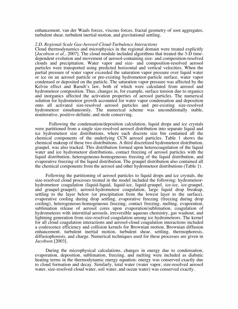
Figure 1 below shows the effect on spectral albedo of different levels of BC in snow. The result suggests that 25 ng/g of BC might reduce the albedo of snow at 550 nm by 2.3%. Clarke and Noone [1985] similarly found that the addition of 25 ng/g of soot to snow decreased snow albedo by about 2.0%. The modeled effect of BC on emissivity is small. For example, at wavelength 7.75 µm, an increase from 0 to 500 ng/g BC increases emissivity by only 0.0005%. Figure 1. Comparison of modeled spectral albedos over snow containing different BC mass mixing ratios when each snow grain contains a single internally-mixed BC inclusion and the rest of the BC in snow is assumed to be externally-mixed (all BC particles in snow are assumed to be 266-nm diameter). The zenith angle (θ) was 72o. From Jacobson [2004].

0

0.2

0.4

0.6

0.8

1

0.2 0.4 0.6 0.8 1

025100250500

Wavelength (µm)

Alb

edo

Snow

r=150 µm, !=72

BC (ng/g)

3. Description of Simulations Nested simulations were run to examine the effects of agriculture and absorption within snow on California climate and air pollution. For both studies, baseline and sensitivity simulations were carried out. For the agricultural study, simulations were run for August 2006; for the snow study, simulations were run for February 1999. The model was run in nested mode from the global to regional scale. Two one-way nested domains were used: a global domain (4o-SN x 5o-WE resolution) and a California domain (0.2ox0.15o ≈ 21.5 km x 14.0 km with the southwest corner grid cell centered at 30.0oN and -126.0oW and 60 SN cells x 75 WE cells). The global domain included 39 sigma-pressure layers between the surface and 0.425 hPa. The nested regional grids included 26 layers between the surface and 103.5 hPa, matching the bottom 26 global-model layers exactly. Each domain included five layers in the bottom 1 km. The nesting time interval for passing meteorological and chemical variables was one hour. The gas and particle emission inventory used was the U.S. National Emission Inventory for 2002 [USEPA, 2006a]. The inventory accounted for over 370,000 stack and fugitive sources, 250,000 area sources, and 1700 source classification code (SCC) categories of onroad and nonroad mobile sources. Pollutants emitted hourly included CO, CH4, paraffins, olefins, formaldehyde, higher aldehydes, toluene, xylene, isoprene, monoterpenes), NO, NO2, HONO, NH3, SO2, SO3, H2SO4, particle black carbon, particle organic carbon, particle sulfate, particle nitrate, and other particulate matter. From the raw U.S. inventory, special inventories were prepared for each model domain. Particle mass emissions were spread over multimodal lognormal distributions. Additional emission types treated in the model were biogenic gases (isoprene, monoterpenes, and other volatile organics from vegetation and nitric oxide from soils), soildust, sea spray,

pollen, spores, and bacteria, NO from lightning, DMS from the oceans, volcanic SO2, many gases and particles from biomass burning, and CO2, H2, and H2O from fossil-fuel combustion and biomass burning. For August 2006, a baseline simulation (with irrigation and current albedo) and two sensitivity simulations (one without irrigation but with current albedo and the other without irrigation and with pre-agriculture albedo) were run. For February 1999, a baseline simulation (with absorption by BC and soildust in snow) and one sensitivity simulation (without absorption in snow) were run. In the February baseline simulation, BC and soildust emissions, evolution, and absorption within snow were treated. In the sensitivity simulation, BC and soildust absorption within snow were not treated. Sources of BC emissions in the model included shipping, aircraft, other fossil fuels, biofuels, and biomass burning. Land-based fossil-fuel soot (BC, OM, and sulfate) emissions were obtained from USEPA [2006] within the U.S. and Bond et al. [2004] outside the U.S.. Shipping BC emissions were obtained by scaling BC emission factors to the sulfur shipping emission rate from Corbett et al. [2003], as described in Jacobson [2006]. Aircraft BC emissions inventory were derived by applying BC emission factors to the 1999 commercial, military, and charter aircraft fuel use data of Sutkus et al. [2001] and Mortlock and Van Alstyne [1998]. Soildust emissions as a function of size, soil type, wind speed, soil moisture, and snow cover were calculated with the method of Marticorena et al. [1997] using soil data from Miller and White [1998].

The global domain simulations were the same for both baseline and sensitivity

California-domain simulations to ensure that errors due to coarser resolution in the global domain did not influence results in the finer California domain.

The model dynamics time steps were 300 s (global domain) and 10 s (California

domain). The time interval for nesting between the domains was 1 hour. Nesting was treated using a five-row buffer layer at each horizontal boundary in each fine domain to relax concentrations and other variables from the coarse domain, as in Jacobson [2005d, Section 21.1.11]. Variables passed at the horizontal boundaries included temperature, specific humidity, wind velocity, gas concentrations (including total water as water vapor), and size- and composition-resolved aerosol concentrations. Clouds themselves were treated with no-flux boundary conditions since total water as water vapor moved across boundaries and could generate new clouds; however, there is no reason why clouds could not be passed across the boundaries as well for future studies.

For February 1999, initial meteorological fields were obtained from National Center for Environmental Prediction (NCEP) reanalysis fields for February 1 1999, at 12 GMT (NCEP, 2003). Aerosol and gas fields in all domains were similarly initialized from background data. U.S. EPA ambient air quality data [USEPA, 2006b]. for O3, CO, NO2, SO2, PM2.5, and PM10 were then assimilated with background values at the initial time. For August 2006, initial meteorological fields were obtained from Global Forecast System (GFS) 1ox1o data. No data assimilation, nudging, or model spinup was performed during any simulation and gas/aerosol fields were initialized from background values. 4. Effects of Agriculture Figure 4 shows baseline and sensitivity simulation results related to agriculture. Each subfigure includes (in the upper right corner), the average parameter value over all land in the figure, which includes land in California and parts of Nevada. Table 2 summarizes statistics from the figures and figures not shown. Statistics over all land rather than irrigated land only are shown since the latter do not capture feedbacks to areas beyond

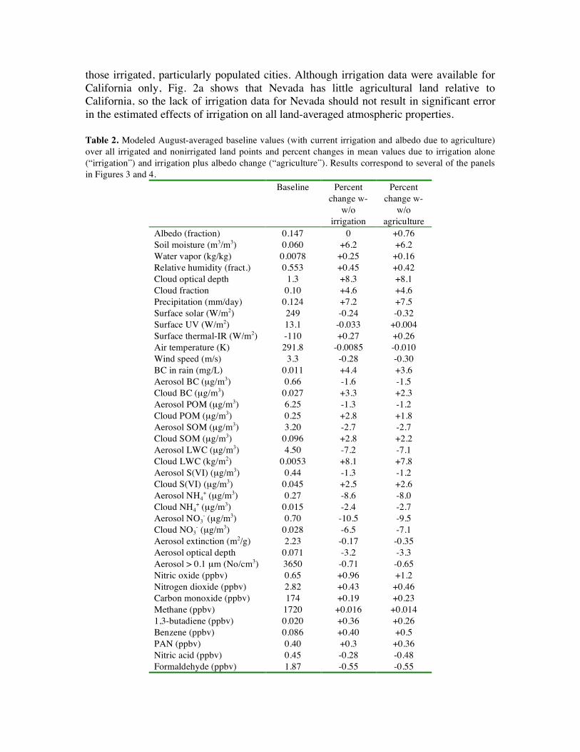
those irrigated, particularly populated cities. Although irrigation data were available for California only, Fig. 2a shows that Nevada has little agricultural land relative to California, so the lack of irrigation data for Nevada should not result in significant error in the estimated effects of irrigation on all land-averaged atmospheric properties. Table 2. Modeled August-averaged baseline values (with current irrigation and albedo due to agriculture) over all irrigated and nonirrigated land points and percent changes in mean values due to irrigation alone (“irrigation”) and irrigation plus albedo change (“agriculture”). Results correspond to several of the panels in Figures 3 and 4.

Baseline Percent change w-

w/o irrigation

Percent change w-

w/o agriculture

Albedo (fraction) 0.147 0 +0.76 Soil moisture (m3/m3) 0.060 +6.2 +6.2 Water vapor (kg/kg) 0.0078 +0.25 +0.16 Relative humidity (fract.) 0.553 +0.45 +0.42 Cloud optical depth 1.3 +8.3 +8.1 Cloud fraction 0.10 +4.6 +4.6 Precipitation (mm/day) 0.124 +7.2 +7.5 Surface solar (W/m2) 249 -0.24 -0.32 Surface UV (W/m2) 13.1 -0.033 +0.004 Surface thermal-IR (W/m2) -110 +0.27 +0.26 Air temperature (K) 291.8 -0.0085 -0.010 Wind speed (m/s) 3.3 -0.28 -0.30 BC in rain (mg/L) 0.011 +4.4 +3.6 Aerosol BC (µg/m3) 0.66 -1.6 -1.5 Cloud BC (µg/m3) 0.027 +3.3 +2.3 Aerosol POM (µg/m3) 6.25 -1.3 -1.2 Cloud POM (µg/m3) 0.25 +2.8 +1.8 Aerosol SOM (µg/m3) 3.20 -2.7 -2.7 Cloud SOM (µg/m3) 0.096 +2.8 +2.2 Aerosol LWC (µg/m3) 4.50 -7.2 -7.1 Cloud LWC (kg/m2) 0.0053 +8.1 +7.8 Aerosol S(VI) (µg/m3) 0.44 -1.3 -1.2 Cloud S(VI) (µg/m3) 0.045 +2.5 +2.6 Aerosol NH4

+ (µg/m3) 0.27 -8.6 -8.0 Cloud NH4

+ (µg/m3) 0.015 -2.4 -2.7 Aerosol NO3

- (µg/m3) 0.70 -10.5 -9.5 Cloud NO3

- (µg/m3) 0.028 -6.5 -7.1 Aerosol extinction (m2/g) 2.23 -0.17 -0.35 Aerosol optical depth 0.071 -3.2 -3.3 Aerosol > 0.1 µm (No/cm3) 3650 -0.71 -0.65 Nitric oxide (ppbv) 0.65 +0.96 +1.2 Nitrogen dioxide (ppbv) 2.82 +0.43 +0.46 Carbon monoxide (ppbv) 174 +0.19 +0.23 Methane (ppbv) 1720 +0.016 +0.014 1,3-butadiene (ppbv) 0.020 +0.36 +0.26 Benzene (ppbv) 0.086 +0.40 +0.5 PAN (ppbv) 0.40 +0.3 +0.36 Nitric acid (ppbv) 0.45 -0.28 -0.48 Formaldehyde (ppbv) 1.87 -0.55 -0.55

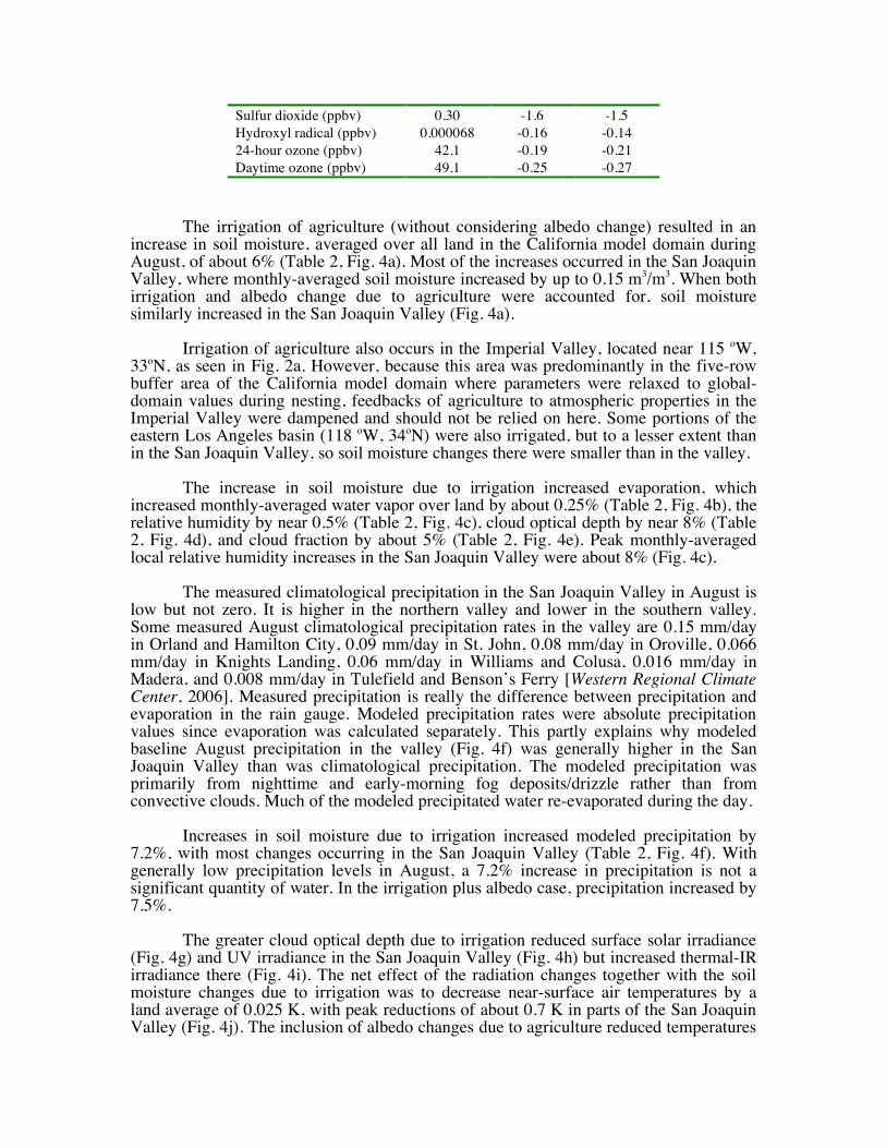
Sulfur dioxide (ppbv) 0.30 -1.6 -1.5 Hydroxyl radical (ppbv) 0.000068 -0.16 -0.14 24-hour ozone (ppbv) 42.1 -0.19 -0.21 Daytime ozone (ppbv) 49.1 -0.25 -0.27

The irrigation of agriculture (without considering albedo change) resulted in an increase in soil moisture, averaged over all land in the California model domain during August, of about 6% (Table 2, Fig. 4a). Most of the increases occurred in the San Joaquin Valley, where monthly-averaged soil moisture increased by up to 0.15 m3/m3. When both irrigation and albedo change due to agriculture were accounted for, soil moisture similarly increased in the San Joaquin Valley (Fig. 4a). Irrigation of agriculture also occurs in the Imperial Valley, located near 115 oW, 33oN, as seen in Fig. 2a. However, because this area was predominantly in the five-row buffer area of the California model domain where parameters were relaxed to global-domain values during nesting, feedbacks of agriculture to atmospheric properties in the Imperial Valley were dampened and should not be relied on here. Some portions of the eastern Los Angeles basin (118 oW, 34oN) were also irrigated, but to a lesser extent than in the San Joaquin Valley, so soil moisture changes there were smaller than in the valley. The increase in soil moisture due to irrigation increased evaporation, which increased monthly-averaged water vapor over land by about 0.25% (Table 2, Fig. 4b), the relative humidity by near 0.5% (Table 2, Fig. 4c), cloud optical depth by near 8% (Table 2, Fig. 4d), and cloud fraction by about 5% (Table 2, Fig. 4e). Peak monthly-averaged local relative humidity increases in the San Joaquin Valley were about 8% (Fig. 4c). The measured climatological precipitation in the San Joaquin Valley in August is low but not zero. It is higher in the northern valley and lower in the southern valley. Some measured August climatological precipitation rates in the valley are 0.15 mm/day in Orland and Hamilton City, 0.09 mm/day in St. John, 0.08 mm/day in Oroville, 0.066 mm/day in Knights Landing, 0.06 mm/day in Williams and Colusa, 0.016 mm/day in Madera, and 0.008 mm/day in Tulefield and Benson’s Ferry [Western Regional Climate Center, 2006]. Measured precipitation is really the difference between precipitation and evaporation in the rain gauge. Modeled precipitation rates were absolute precipitation values since evaporation was calculated separately. This partly explains why modeled baseline August precipitation in the valley (Fig. 4f) was generally higher in the San Joaquin Valley than was climatological precipitation. The modeled precipitation was primarily from nighttime and early-morning fog deposits/drizzle rather than from convective clouds. Much of the modeled precipitated water re-evaporated during the day. Increases in soil moisture due to irrigation increased modeled precipitation by 7.2%, with most changes occurring in the San Joaquin Valley (Table 2, Fig. 4f). With generally low precipitation levels in August, a 7.2% increase in precipitation is not a significant quantity of water. In the irrigation plus albedo case, precipitation increased by 7.5%. The greater cloud optical depth due to irrigation reduced surface solar irradiance (Fig. 4g) and UV irradiance in the San Joaquin Valley (Fig. 4h) but increased thermal-IR irradiance there (Fig. 4i). The net effect of the radiation changes together with the soil moisture changes due to irrigation was to decrease near-surface air temperatures by a land average of 0.025 K, with peak reductions of about 0.7 K in parts of the San Joaquin Valley (Fig. 4j). The inclusion of albedo changes due to agriculture reduced temperatures

further, by a total land-average of 0.03 K (Fig. 4j). Thus, the net increase in albedo of up to 6% locally in California due to agriculture (Fig. 3b) had a measurable impact on land-averaged temperature. The effect of irrigation on air temperatures was net cooling; however, irrigation generally warmed the air slightly at night but cooled it to a greater extent during the day (Fig. 5), reducing the magnitudes of both temperature maximums and minimums. The net cooling of near-surface air and increase in precipitation due to agriculture (irrigation plus albedo change) found here is consistent in direction with the data analysis results of Barnston and Schickedanz [1984] but also with Moore and Rojstaczer [2001], who concluded that the magnitude of precipitation change due to agriculture may be small. The cooling due to agriculture is also consistent with results from Adegoke et al. [2003], Boucher et al. [2004], Snyder et al. [2006], and Lobell et al. [2006]. Because agriculture appears to have increased rather than decreased the albedo over most of the San Joaquin Valley, the net warming found in the valley by Christy et al. [2006] may be due to other factors (e.g., anthropogenic greenhouse gas and absorbing particle warming) rather than an increase in agriculture as speculated therein. The observed warming in the valley is unlikely to be due to the sum of all anthropogenic aerosol particles; Jacobson and Kaufman [2006], for example, found a net cooling (nighttime warming and greater daytime cooling) due to such particles in the San Joaquin Valley. Although black carbon in aerosol particles causes warming, it is dominated by larger amounts of scattering aerosol particles. The increase in drizzle in the San Joaquin Valley due to irrigation increased the concentration of pollutants in rainwater, increasing wet removal of these pollutants. For example, irrigation alone increased the concentration of BC in cloud water by about 3.3% (Table 2) and rainwater by about 4.4% (Table 2, Fig. 4k) and decreased it in air by about 1.6% (Table 2, Fig. 4l) on average over all land, but mostly in the San Joaquin Valley. Due to enhanced drizzle, irrigation similarly decreased aerosol POM, SOM, S(VI), NH4

+, and NO3

- (Table 2). Although a higher relative humidity (Table 2) tended to increase aerosol liquid water content (ALWC), the removal of hydrating aerosol constituents caused a net decrease in ALWC (Table 2). The net effect of irrigation, therefore, in the San Joaquin Valley was to decrease aerosol extinction (Table 2), optical depth (Table 2, Fig. 4m), and number (Table 2, Fig. 4n). Irrigation slightly increased the near-surface mixing ratios of low-solubility, slowly reacting gases, such as CO, CH4 (Table 2) by reducing the mixing depth and decreasing the near-surface wind speed (Table 2). It reduced the mixing depth by cooling the ground (Table 2, Fig. 3h), thereby increasing stability. The enhanced stability reduced turbulent kinetic energy and shearing stress, which reduced vertical transport of faster winds aloft to the surface. Irrigation slightly increased the near-surface mixing ratios of low-solubility, slowly reacting gases, such as CO, CH4 (Table 2) by (a) cooling the ground (Table 2, Fig. 4j), thereby increasing stability and reducing the mixing depth, and (b) decreasing the near-surface wind speed (Table 2, Fig. 4t). Irrigation reduced wind speed by cooling the surface, thereby increasing stability, reducing turbulent kinetic energy, shearing stress, and the vertical transport of faster winds aloft to the surface. Irrigation decreased the near-surface mixing ratios of soluble gases, such as HNO3 (Fig. 4q), HCHO (Fig. 4r), and SO2 (Table 2) by increasing cloud liquid water and precipitation. The reduction in aldehydes and UV radiation (Fig. 4h) reduced OH in the valley (Fig. 4s). The reduction in UV radiation and increase in near-surface NO and NO2 (Table 2, Fig. 4p) in the northern San Joaquin Valley helped to decrease near-surface ozone in the northern valley (Fig. 4o) and increase PAN, on average over land (Table 2).

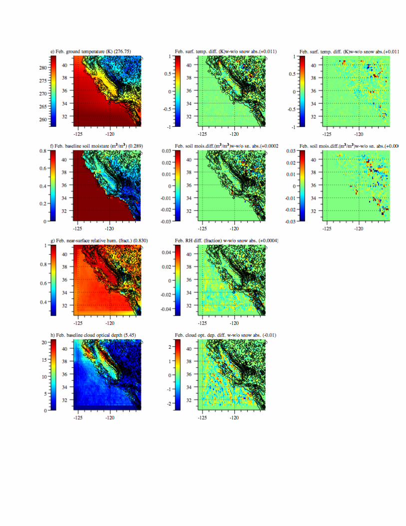
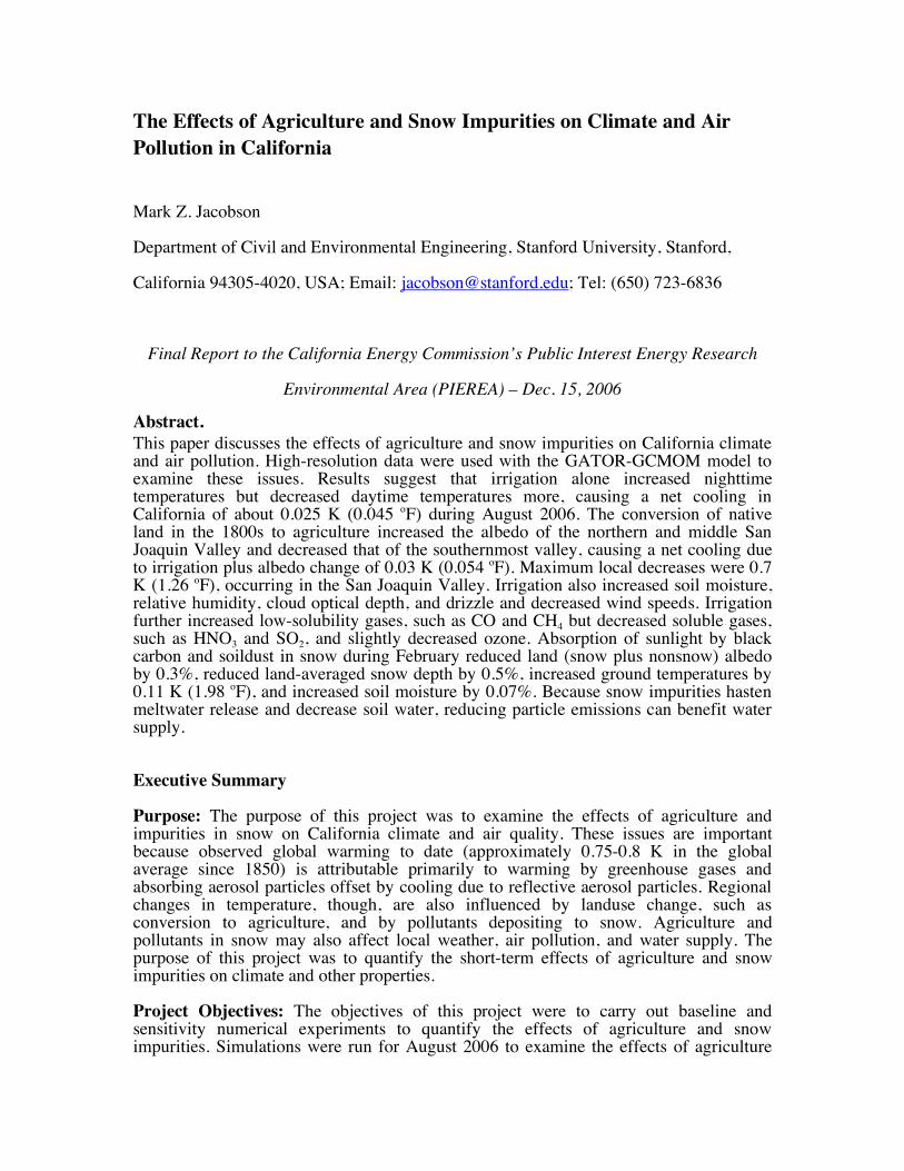
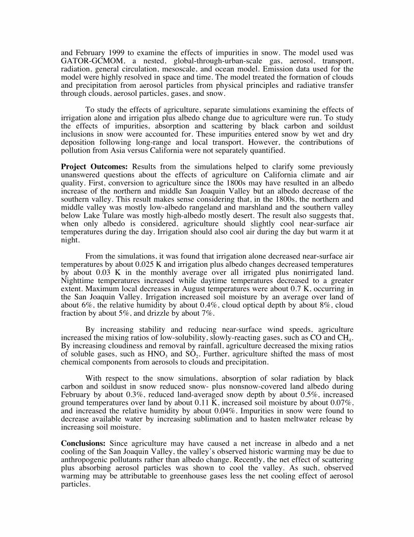
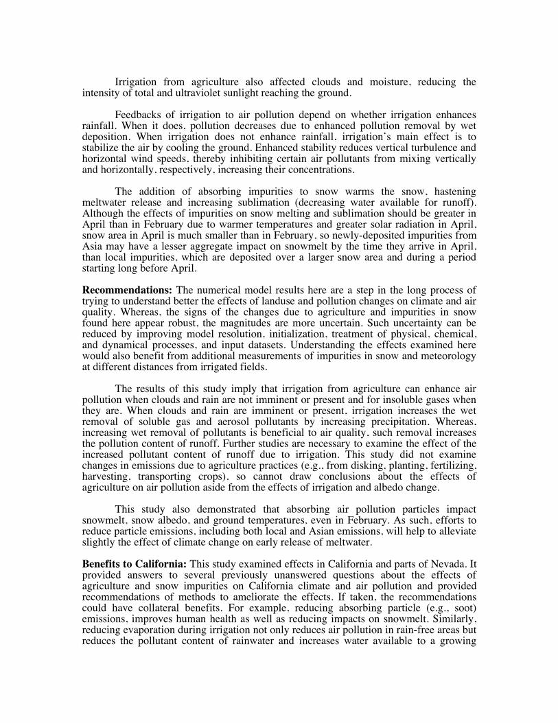
A decrease in nitrogen oxides in the southern valley (Fig. 4p) contributed to an ozone increase there (Fig. 4o). Table 2 indicates that percent changes in several parameters due to irrigation were relatively small. This might suggest that the magnitude and direction of the modeled changes could be random. However, if the changes were random, the results would change randomly upon a change in the initial conditions or of a parameterization in the model and would not follow what might be expected from physical principles. However, Table 2 indicates that, when a second sensitivity test was run for each domain (e.g., when both albedo and irrigation were perturbed) the percent changes were close to those when only irrigation was perturbed. Further changes in both sensitivities could be explained in terms of physical principles. As such, it appears unlikely that the sign of the changes found were random or noise but were real responses to irrigation and/or albedo changes. The magnitudes of the changes are more uncertain and would undoubtedly change further upon an improvement in model resolution and physical processes treated. 5. Effects of Impurities in Snow February 1999 was a moderately wet year in Northern California but dry in the Southern part of the state (Fig. 6). Most precipitation occurred along the northern coast and in the Sierra Nevada Mountains. The model was able to predict the locations of strong and weak precipitation as well as the magnitude in many locations although it overpredicted the magnitude in the Sierras by about a third (Fig. 6). Part of this error may be due to coarse model resolution (21.5 km x 14.0 km) and to initialization with the coarsely-resolved NCEP reanalysis (2.5o x 2.5 o). Table 3. Summary of February modeled mean baseline values over all land points in the model domain and percent changes in mean values due to BC and soildust absorption in snow. Data correspond to Figure 7.

Mean baseline value

(with absorption in snow)

Mean percent change with minus without absorption in snow

Snow depth (m) 0.0217 -0.41 Albedo (fraction) 0.247 -0.32 BC in air (µg/m3) 0.287 -0.02 BC in cloud particles (µg/m3) 0.027 +0.27 BC in rain (mg/L) 0.011 +0.20 BC in snow (mg/L) 0.0023 -1.8 Soildust in air (µg/m3) 0.187 -3.1 Soildust in cloud part. (µg/m3) 0.009 -3.6 Soildust in rain (mg/L) 0.082 +2.1 Soildust in snow (mg/L) 0.058 +4.3 Ground temperature (K) 276.75 +0.004 Soil moisture (m3/m3) 0.289 +0.07 Relative humidity (fraction) 0.83 +0.048 Cloud optical depth 5.45 -0.18

Most of the modeled snow fell in the Sierras although small amount fell in Northern and Eastern Nevada as well (Fig. 7a), as indicated by the higher albedos there

(Fig. 7b). Black carbon and soildust in the model were tracked through aerosols, clouds, rain, and snow (Figs. 7c, 7d). Both entered snow by wet and dry deposition. While nearly all BC in the model was anthropogenic, most soildust was natural and produced by the wind passing over loose sand or dirt. Absorption of solar radiation by BC and soildust together in snow reduced snow depth by about 0.4% (Table 3, Fig. 7a) and surface albedo by about 0.32% (Table 3, Fig. 7b) in February in the California domain over all land points (snow covered and non-snow-covered). Maximum snow depth and albedo decreases over snow were 2% and 4%, respectively. For comparison, Jacobson [2004] calculated that BC alone reduced snow and sea ice albedo by 0.4% in the annual and global average and 1% in the Northern Hemisphere. The larger effects on the global scale were due to the fact that the feedbacks operated over a much longer time in that study. Also, the Arctic and Northern Europe/Asia, where most of the black carbon effects occurred on the global scale, have nearby sources of BC (e.g., Europe and Asia) greater in magnitude than does California (mostly the San Joaquin Valley, Los Angeles, and San Francisco). The increased absorption by BC and soildust in snow increased the modeled ground temperature in February over all land by about 0.11 K (0.004%) (Table 3, Fig. 7e). For comparison, the global and annual average increase in near-surface air temperatures due to BC absorption alone in snow was about 0.06 K [Jacobson, 2004]. The reduction in snow due to absorption was compensated for in part by increases in meltwater and water vapor. Snow absorption increased soil moisture by about 0.07% (Table 3, Fig. 7f), water vapor by about 0.1%, and the relative humidity by about 0.05% (Table 3, Fig. 7g). The increase in soil moisture suggests a hastening of the release of meltwater due to absorption by impurities in snow. The increase in water vapor together with the loss in snow depth suggests a net reduction in water supply due to such impurities. The rate of snowmelt depends on ambient temperatures and temperature changes due to impurities in snow. In April, ambient temperatures are higher so more snow melts than in February, as indicated by the snow depth statistics discussed in Section 1. Similarly, the same level of impurities in snow speeds melting of snow in April more than in February because incident solar radiation, thus solar absorption and thermal-infrared heating by impurities, is greater in April. Finally, because less snowfall occurs in April than in February, more impurities can accumulate on top of snow without being buried by new snow in April. On the other hand since more snow is present in February, impurities in snow cause feedbacks over a larger region in February than in April. Overall, it is estimated that the results here for February may underestimate the effects of impurities on snowmelt relative to April. Finally, the higher water vapor in the San Joaquin Valley resulted in a slight increase in cloud optical depth there (Fig. 7h), although the land-averaged change in optical depth was negative (Table 3).

6. Conclusions This paper discussed the effects of irrigation and albedo change due to agriculture on California weather, climate, and air pollution, and the effects of black carbon and soildust absorption within snow on snowmelt and the subsequent feedback to California climate. Numerical simulations were run for August 2006 to examine the first issue and February 1999 to examine the second issue. Satellite albedo data and irrigation data were obtained to examine the first issue. An inversion method was combined with the satellite data to estimate California’s albedo in the absence of agriculture. It was found that agriculture may have increased the albedo of the northern and middle San Joaquin Valley but decreased the albedo of the southern valley relative to the albedo in the 1800s. Such a result implies that, when only albedo is considered, agriculture should cause a slight cooling of the valley. Irrigation should also cause cooling during the day but a warming at night. From the numerical simulations, it was found that irrigation alone decreased near-surface air temperatures by about 0.025 K and irrigation plus albedo changes decreased temperatures by about 0.03 K in the monthly average over land in the model domain (covering California and parts of Nevada). Nighttime temperatures increased while daytime temperatures decreased to a greater extent. Maximum local decreases in August temperatures were about 0.7 K, occurring in the San Joaquin Valley. Since agriculture caused a net summer cooling of the San Joaquin Valley, the valley’s observed historic warming appears more likely due to anthropogenic greenhouse gas buildup than to agriculture. Irrigation increased soil moisture by an average over land of about 6%, the relative humidity by about 0.4%, cloud optical depth by about 8%, cloud fraction by about 5%, and drizzle by about 7%. Increased stability due to irrigation decreased wind speeds. Both factors increased the near-surface mixing ratios of low-solubility, slowly-reacting gases, such as CO and CH4. By increasing cloudiness and wet removal, agriculture decreased the mixing ratios of soluble gases, such as HNO3 and SO2. Thus, irrigation reduced primary pollutant concentrations when precipitation or drizzle was imminent or present but increased such pollution when precipitation was absent. Reductions in UV radiation and increases in nitrogen oxides due to irrigation slightly decreased ozone in California. With respect to the effects of impurities in snow, absorption of solar radiation by black carbon and soildust in snow reduced land albedo in February by about 0.3%, reduced land-averaged snow depth by about 0.5%, increased ground temperatures over land by about 0.11 K, increased soil moisture by about 0.07%, and increased the relative humidity by about 0.04% over land. This result implies that impurities in snow may decrease water supply by increasing sublimation and may hasten the release of meltwater. Although the effects of impurities on snow melting should be greater in April than in February due to warmer temperatures and greater solar radiation in April, snow area in April is much lower than in February, so newly-deposited impurities from Asia may have a lesser aggregate impact on snowmelt by the time they arrive in April, than local impurities, which are deposited over a larger snow area and over a longer period prior to April. Nevertheless, this study implies that efforts to reduce both local and Asian particle emissions will help to alleviate slightly the effect of climate change on early release of meltwater. Reducing emissions have the additional benefit of improving human health. Whereas, the modeled signs of changes due to agriculture and impurities in snow may be relatively reliable, the magnitudes are more uncertain. Such uncertainty can be

reduced by improving model resolution, initialization, treatment of physical, chemical, and dynamical processes, and input datasets. Acknowledgments This work was funded by California Energy Commission’s Public Interest Energy Research Environmental Area (PIEREA) program. I would like to thank Guido Franco for helpful comments and William Salas for providing irrigation data. Legal Notice This report was prepared as a result of work sponsored by the California Energy Commission (Commission) and the University of California (UC). It does not necessarily represent the views of the Commission, UC, their employees, or the State of California. The Commission, the State of California, its employees, and UC make no warranty, express or implied, and assume no legal liability for the information in this report; nor does any party represent that the use of this information will not infringe upon privately owned rights. This report has not been approved or disapproved by the Commission or UC, nor has been approved or disapproved by the Commission or UC, nor has the Commission or UC passed upon the accuracy or adequacy of the information in this report.

References Adegoke, J.O., R.A.S. Pielke, J.L. Eastman, R. Mahmood, and K.G. Hubbard, Impact of

irrigation on midsummer surface fluxes and temperature under dry synoptic conditions: A regional atmospheric model study of the U.S. High Plains, Monthly Weather Review, 131, 556-564, 2003.

Aoki, T., T. Aoki, M. Fukabori, A. Hachikubo, Y. Tachibana, and F. Nishio, Effects of snow physical parameters on spectral albedo and bi-directional reflectance of snow surface, J. Geophys. Res., 105, 10,219-10,236, 2000.

Arakawa, A., and V. R. Lamb, A potential enstrophy and energy conserving scheme for the shallow water equations, Mon. Wea. Rev., 109, 18-36, 1981.

Barnston, A., and P.T. Schickedanz, The effect of irrigation on warm season precipitation in the southern Great Plains, J. Climate Appl. Meteor., 23, 865-888, 1984.

Bond, T.C., Streets, D.G., Yarber, K.F., Nelson, S.M., Woo, J.-H. & Klimont, Z., A technology-based global inventory of black and organic carbon emissions from combustion, J. Geophys. Res., 109, D14203, doi: 10.1029/2003JD003697, 2004.

Boucher, O., G. Myhre, A. Myhre, Direct human influence of irrigation on atmospheric water vapor and climate, Climate Dynamics, 22, 597-603, 2004.

Christy, J.R., W.B. Norris, K. Redmond, K.P. Gallo, Methodology and results of calculating Central California surface temperature trends: Evidence of human-induced climate change? J. Clim., 19, 548-563, 2005.

Chylek, P., V. Ramaswamy, and V. Srivastava, Albedo of soot-contaminated snow, J. Geophys. Res., 88, 10,837-10,843, 1983.

Chylek, P., V. Srivastava, L. Cahenzli, R.G. Pinnick, R.L. Dod, T. Novakov, T.L. Cook, and B.D. Hinds, Aerosol and graphitic carbon content of snow, J. Geophys. Res., 92, 9801-9809, 1987.

Clark, R.N., and P.G. Lucey, Spectral properties of ice-particulate mixtures and implications for remote sensing, 1, Intimate mixtures, J. Geophys. Res., 89, 6341-6348, 1984.

Clarke, A. D., and K. J. Noone, Soot in the Arctic snowpack: A cause for perturbations in radiative transfer, Atmos. Environ., 19, 2045-2053, 1985.

Corbett, J.J.; Koehler, H.W. J. Geophys. Res., 108 (D20), 4650, doi:10.1029/2003JD003751, 2003.

Cuenca, R.H., M. Ek, and L. Mahrt, Impact of soil water property parameterization on atmospheric boundary layer simulation, J. Geophys. Res., 101, 7269-7277, 1996.

Emori, S., The interaction of cumulus convection with soil moisture distribution: An idealized simulation, J. Geophys. Res., 103, 8873-8884, 1998.

Fennessy, M.J., and J. Shukla, Impact of initial soil wetness on seasonal atmospheric prediction, J. Clim, 12, 3167, 1999.

Flanner, M.G., C.S. Zender, and J.T. Randerson, Present day climate forcing and response from black carbon in snow, J. Geophys. Res., in press, 2006, www.ess.uci.edu/~zender/.

Fuller, K. A., W. C. Malm, and S. M. Kreidenweis, Effects of mixing on extinction by carbonaceous particles, J. Geophys. Res., 104, 15,941-15,954, 1999.

Giambelluca, T.W., D. Holscher, T.X. Bastos, R.R. Frazao, M.A. Nullet, and A.D. Ziegler, Observations of albedo and radiation balance over postforest land surfaces in the Eastern Amazon basin, J. Clim., 10, 919-928, 1997.

Global Forecast System (GFS), National Center for Environmental Prediction, http://nomads.ncdc.noaa.gov/data/gfs-avn-hi/, 2006.

Goldstein, A. H., D. B. Millet, M. McKay, L. Jaegle, L. Horowitz, O. Cooper, R. Hudman, D. Jacob, S. Oltmans and A. Clarke, Impact of Asian emissions on observations at Trinidad Head, California, during ITCT 2K2, J. Geophys. Res., 109, D23S17, doi:10.1029/2003JD004406, 2004.

Grenfell, T. C., S. G. Warren, and P. C. Mullen, Reflection of solar radiation by the Antarctic snow surface at ultraviolet, visible, and near-infrared wavelengths, J. Geophys. Res., 99, 18,669-18,684, 1994.

Grenfell, T.C., B. Light, and M. Sturm, Spatial distribution and radiative effects of soot in the snow and sea ice during the SHEBA experiment, J. Geophys. Res., 107, 10.1029/2000JC000414, 2002.

Gribbon, P.W.F., Cryoconite holes on Sermikavsak, West Greenland, J. Glaciol, 22, 177-181, 1979.

Gutman, G., G. Ohring, D. Tarpley, and R. Ambroziak, Albedo of the U.S. Great Plains as determined from NOAA-9 AVHRR data, J. Clim. 2, 608-617, 1989.

Hansen, J. and L. Nazarenko, Soot climate forcing via snow and ice albedos, Proc. Natl. Acad. Sci., doi/10.1073/pnas.2237157100, 2003.

Hansen, J., et al., Efficacy of climate forcing, J. Geophys. Res., 110, D18104, doi:10.1029/2005JD005776, 2005.

Higuchi, K., and A. Nagoshi, Effect of particulate matter in surface snow layers on the albedo of perennial snow patches, IAHS AISH Publ., 118, 95-97, 1977.

Jacobson, M. Z., Improvement of SMVGEAR II on vector and scalar machines through absolute error tolerance control. Atmos. Environ., 32, 791–796, 1998b.

Jacobson, M. Z., Development and application of a new air pollution modeling system. Part II: Aerosol module structure and design, Atmos. Environ., 31A, 131-144, 1997a.

Jacobson, M. Z., Development and application of a new air pollution modeling system. Part III: Aerosol-phase simulations, Atmos. Environ., 31A, 587-608, 1997b.

Jacobson, M. Z., Studying the effects of soil moisture on ozone, temperatures, and winds in Los Angeles, J. Appl. Meteorol., 38, 607-616, 1999.

Jacobson, M. Z., GATOR-GCMM: A global through urban scale air pollution and weather forecast model. 1. Model design and treatment of subgrid soil, vegetation, roads, rooftops, water, sea ice, and snow., J. Geophys. Res., 106, 5385-5402, 2001a.

Jacobson, M. Z., GATOR-GCMM: 2. A study of day- and nighttime ozone layers aloft, ozone in national parks, and weather during the SARMAP Field Campaign, J. Geophys. Res., 106, 5403-5420, 2001b.

Jacobson, M. Z., Control of fossil-fuel particulate black carbon plus organic matter, possibly the most effective method of slowing global warming, J. Geophys. Res., 107, (D19), 4410, doi:10.1029/ 2001JD001376, 2002a.

Jacobson, M. Z., Analysis of aerosol interactions with numerical techniques for solving coagulation, nucleation, condensation, dissolution, and reversible chemistry among

multiple size distributions, J. Geophys. Res., 107 (D19), 4366, doi:10.1029/ 2001JD002044, 2002b.

Jacobson, M. Z., Development of mixed-phase clouds from multiple aerosol size distributions and the effect of the clouds on aerosol removal, J. Geophys. Res., 108 (D8), 4245, doi:10.1029/2002JD002691, 2003.

Jacobson, M.Z., The climate response of fossil-fuel and biofuel soot, accounting for soot’s feedback to snow and sea ice albedo and emissivity, J. Geophys. Res., 109, D21201, doi:10.1029/2004JD004945, 2004.

Jacobson, M.Z., A solution to the problem of nonequilibrium acid/base gas-particle transfer at long time step, Aerosol Sci. Technol, 39, 92-103, 2005a.

Jacobson, M.Z., A refined method of parameterizing absorption coefficients among multiple gases simultaneously from line-by-line data, J. Atmos. Sci., 62, 506-517, 2005b.

Jacobson, M.Z., Studying ocean acidification with conservative, stable numerical schemes for nonequilibrium air-ocean exchange and ocean equilibrium chemistry, J. Geophys. Res., 110, D07302, doi:10.1029/2004JD005220, 2005c.

Jacobson, M.Z., Fundamentals of Atmospheric Modeling, Second Edition, Cambridge University Press, New York, 813 pp., 2005d.

Jacobson, M.Z., Effects of absorption by soot inclusions within clouds and precipitation on global climate, J. Phys. Chem., 110, 6860-6873, 2006.

Jacobson, M.Z., Y.J. Kaufman, Y. Rudich, Examining feedbacks of aerosols to urban climate with a model that treats 3-D clouds with aerosol inclusions, J. Geophys. Res., in review, 2007, www.stanford.edu/group/efmh/jacobson/iiie.html.

Jacobson, M.Z., and Y.J. Kaufman, Wind reduction by aerosol particles, Geophys. Res. Letters, 33 (24), doi:10.1029/2006GL027838, 2006.

Kahrl, W.L., ed., The California Water Atlas, Governor’s Office of Planning and Research, Sacramento, William Kaufmann, 1979.

Ketefian G., and M.Z. Jacobson, Development and application of a 2-D potential-enstrophy-, energy-, and mass-conserving mixed-layer ocean model with arbitrary boundaries, Mon. Weath. Rev., in review, 2007, http://www.stanford.edu/group/efmh/gsk/index.htm.

Krekov, G. M., Models of Atmospheric Aerosols. In Aerosol Effects on Climate. S. G. Jennings, ed., U. of Arizona Press, Tucson, Ariz., pp. 9-72, 1993.

Lanicci, J. M., T. N. Carlson, and T. T. Warner, Sensitivity of the Great Plains severe-storm environment to soil-moisture distribution, Mon. Wea. Rev., 115, 2660-2673, 1987.

Light, B., H. Eicken, G. A. Maykut, and T. C. Grenfell, The effect of included particulates on the spectral albedo of sea ice, J. Geophys. Res., 103, 27,739-27,752, 1998.

Liu W., P. K. Hopke, R. A. VanCuren, Origins of fine aerosol mass in the western United States using positive matrix factorization, J. Geophys. Res., 108 (D23), 4716, doi:10.1029/2003JD003678, 2003.

Lobell, D.B., G. Bala, and P.B. Duffy, Biogeophysical impacts of cropland management changes on climate, Geophys. Res. Lett., 33, L06708, doi:10.1029/2005GL025492, 2006.

Lu, R., and R. P. Turco, Air pollutant transport in a coastal environment, II, Three-dimensional simulations over Los Angeles basin, Atmos. Environ., 29, 1499-1518, 1995.

Mahfouf, J.-F., E. Richard, and P. Mascart, The influence of soil and vegetation on the development of mesoscale circulations. J. Appl. Meteorol., 26, 1483-1495, 1987.

Maricq, M., D. H. Podsiadlik, and R. E. Chase, Size distributions of motor vehicle exhaust PM: A comparison between ELPI and SMPS measurements, Aerosol Sci. Technol, 33, 239-260, 2000.

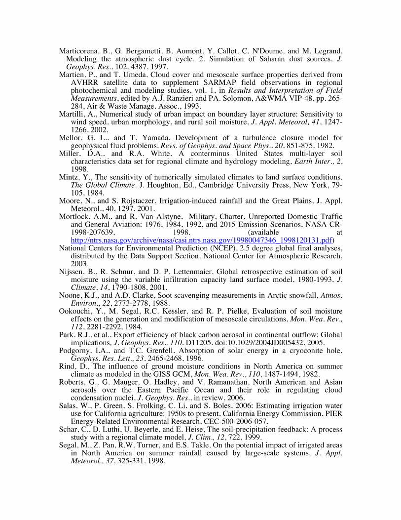
Marticorena, B., G. Bergametti, B. Aumont, Y. Callot, C. N'Doume, and M. Legrand, Modeling the atmospheric dust cycle. 2. Simulation of Saharan dust sources, J. Geophys. Res., 102, 4387, 1997.

Martien, P., and T. Umeda, Cloud cover and mesoscale surface properties derived from AVHRR satellite data to supplement SARMAP field observations in regional photochemical and modeling studies, vol. 1, in Results and Interpretation of Field Measurements, edited by A.J. Ranzieri and PA. Solomon, A&WMA VIP-48, pp. 265-284, Air & Waste Manage. Assoc., 1993.

Martilli, A., Numerical study of urban impact on boundary layer structure: Sensitivity to wind speed, urban morphology, and rural soil moisture, J. Appl. Meteorol, 41, 1247-1266, 2002.

Mellor, G. L., and T. Yamada, Development of a turbulence closure model for geophysical fluid problems, Revs. of Geophys. and Space Phys., 20, 851-875, 1982.

Miller, D.A., and R.A. White, A conterminus United States multi-layer soil characteristics data set for regional climate and hydrology modeling, Earth Inter., 2, 1998.

Mintz, Y., The sensitivity of numerically simulated climates to land surface conditions. The Global Climate. J. Houghton, Ed., Cambridge University Press, New York, 79-105, 1984.

Moore, N., and S. Rojstaczer, Irrigation-induced rainfall and the Great Plains, J. Appl. Meteorol., 40, 1297, 2001.

Mortlock, A.M., and R. Van Alstyne, Military, Charter, Unreported Domestic Traffic and General Aviation: 1976, 1984, 1992, and 2015 Emission Scenarios, NASA CR- 1998-207639, 1998. (available at http://ntrs.nasa.gov/archive/nasa/casi.ntrs.nasa.gov/19980047346_1998120131.pdf)

National Centers for Environmental Prediction (NCEP), 2.5 degree global final analyses, distributed by the Data Support Section, National Center for Atmospheric Research, 2003.

Nijssen, B., R. Schnur, and D. P. Lettenmaier, Global retrospective estimation of soil moisture using the variable infiltration capacity land surface model, 1980-1993, J. Climate, 14, 1790-1808, 2001.

Noone, K.J., and A.D. Clarke, Soot scavenging measurements in Arctic snowfall, Atmos. Environ., 22, 2773-2778, 1988.

Ookouchi, Y., M. Segal, R.C. Kessler, and R. P. Pielke, Evaluation of soil moisture effects on the generation and modification of mesoscale circulations, Mon. Wea. Rev., 112, 2281-2292, 1984.

Park, R.J., et al., Export efficiency of black carbon aerosol in continental outflow: Global implications, J. Geophys. Res., 110, D11205, doi:10.1029/2004JD005432, 2005.

Podgorny, I.A., and T.C. Grenfell, Absorption of solar energy in a cryoconite hole, Geophys. Res. Lett., 23, 2465-2468, 1996.

Rind, D., The influence of ground moisture conditions in North America on summer climate as modeled in the GISS GCM, Mon. Wea. Rev., 110, 1487-1494, 1982.

Roberts, G., G. Mauger, O. Hadley, and V. Ramanathan, North American and Asian aerosols over the Eastern Pacific Ocean and their role in regulating cloud condensation nuclei, J. Geophys. Res., in review, 2006.

Salas, W., P. Green, S. Frolking, C. Li, and S. Boles, 2006: Estimating irrigation water use for California agriculture: 1950s to present, California Energy Commission, PIER Energy-Related Environmental Research, CEC-500-2006-057.

Schar, C., D. Luthi, U. Beyerle, and E. Heise, The soil-precipitation feedback: A process study with a regional climate model, J. Clim., 12, 722, 1999.

Segal, M., Z. Pan, R.W. Turner, and E.S. Takle, On the potential impact of irrigated areas in North America on summer rainfall caused by large-scale systems, J. Appl. Meteorol., 37, 325-331, 1998.

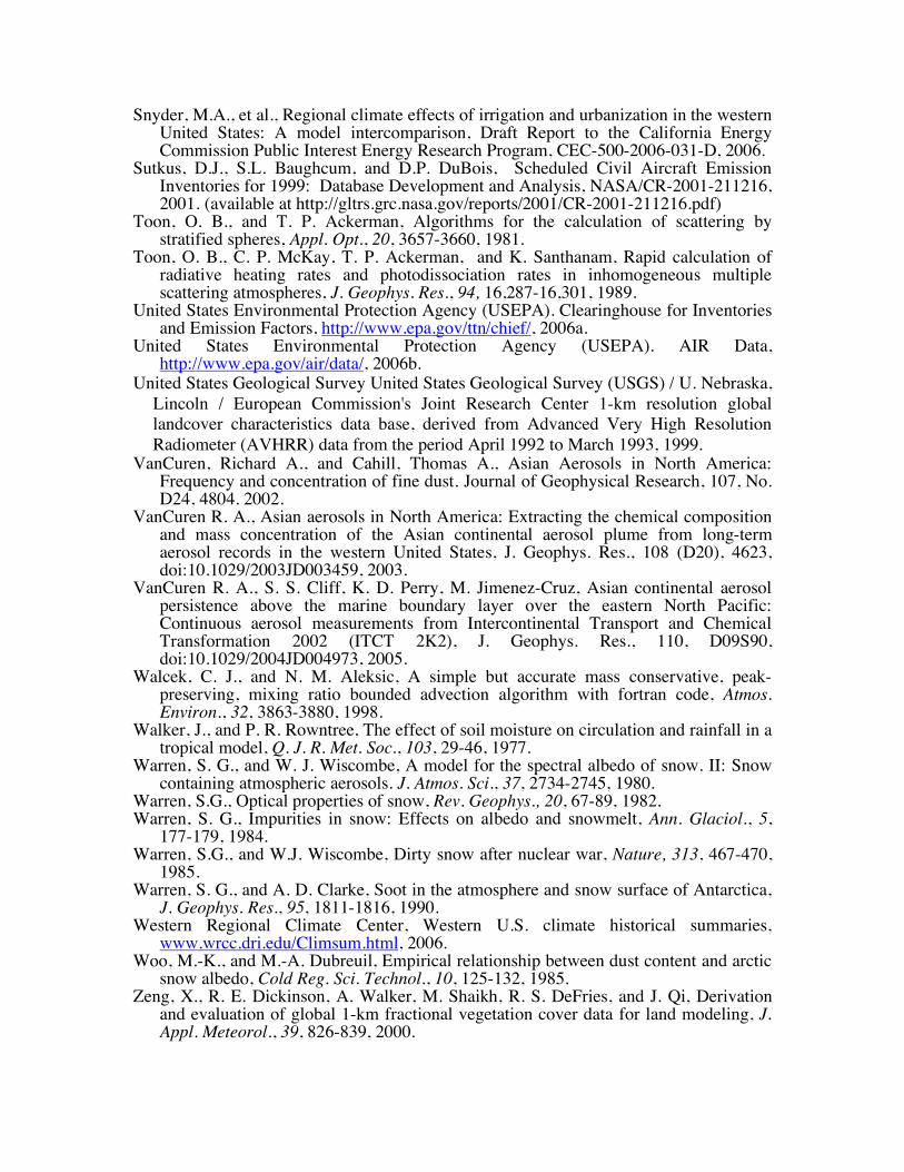
Snyder, M.A., et al., Regional climate effects of irrigation and urbanization in the western United States: A model intercomparison, Draft Report to the California Energy Commission Public Interest Energy Research Program, CEC-500-2006-031-D, 2006.

Sutkus, D.J., S.L. Baughcum, and D.P. DuBois, Scheduled Civil Aircraft Emission Inventories for 1999: Database Development and Analysis, NASA/CR-2001-211216, 2001. (available at http://gltrs.grc.nasa.gov/reports/2001/CR-2001-211216.pdf)

Toon, O. B., and T. P. Ackerman, Algorithms for the calculation of scattering by stratified spheres, Appl. Opt., 20, 3657-3660, 1981.

Toon, O. B., C. P. McKay, T. P. Ackerman, and K. Santhanam, Rapid calculation of radiative heating rates and photodissociation rates in inhomogeneous multiple scattering atmospheres, J. Geophys. Res., 94, 16,287-16,301, 1989.

United States Environmental Protection Agency (USEPA). Clearinghouse for Inventories and Emission Factors, http://www.epa.gov/ttn/chief/, 2006a.

United States Environmental Protection Agency (USEPA). AIR Data, http://www.epa.gov/air/data/, 2006b.

United States Geological Survey United States Geological Survey (USGS) / U. Nebraska, Lincoln / European Commission's Joint Research Center 1-km resolution global landcover characteristics data base, derived from Advanced Very High Resolution Radiometer (AVHRR) data from the period April 1992 to March 1993, 1999.

VanCuren, Richard A., and Cahill, Thomas A., Asian Aerosols in North America: Frequency and concentration of fine dust. Journal of Geophysical Research, 107, No. D24, 4804. 2002.

VanCuren R. A., Asian aerosols in North America: Extracting the chemical composition and mass concentration of the Asian continental aerosol plume from long-term aerosol records in the western United States, J. Geophys. Res., 108 (D20), 4623, doi:10.1029/2003JD003459, 2003.

VanCuren R. A., S. S. Cliff, K. D. Perry, M. Jimenez-Cruz, Asian continental aerosol persistence above the marine boundary layer over the eastern North Pacific: Continuous aerosol measurements from Intercontinental Transport and Chemical Transformation 2002 (ITCT 2K2), J. Geophys. Res., 110, D09S90, doi:10.1029/2004JD004973, 2005.

Walcek, C. J., and N. M. Aleksic, A simple but accurate mass conservative, peak-preserving, mixing ratio bounded advection algorithm with fortran code, Atmos. Environ., 32, 3863-3880, 1998.

Walker, J., and P. R. Rowntree, The effect of soil moisture on circulation and rainfall in a tropical model, Q. J. R. Met. Soc., 103, 29-46, 1977.

Warren, S. G., and W. J. Wiscombe, A model for the spectral albedo of snow. II: Snow containing atmospheric aerosols. J. Atmos. Sci., 37, 2734-2745, 1980.

Warren, S.G., Optical properties of snow, Rev. Geophys., 20, 67-89, 1982. Warren, S. G., Impurities in snow: Effects on albedo and snowmelt, Ann. Glaciol., 5,

177-179, 1984. Warren, S.G., and W.J. Wiscombe, Dirty snow after nuclear war, Nature, 313, 467-470,

1985. Warren, S. G., and A. D. Clarke, Soot in the atmosphere and snow surface of Antarctica,

J. Geophys. Res., 95, 1811-1816, 1990. Western Regional Climate Center, Western U.S. climate historical summaries,

www.wrcc.dri.edu/Climsum.html, 2006. Woo, M.-K., and M.-A. Dubreuil, Empirical relationship between dust content and arctic

snow albedo, Cold Reg. Sci. Technol., 10, 125-132, 1985. Zeng, X., R. E. Dickinson, A. Walker, M. Shaikh, R. S. DeFries, and J. Qi, Derivation

and evaluation of global 1-km fractional vegetation cover data for land modeling, J. Appl. Meteorol., 39, 826-839, 2000.

Zhang, D., and R.A. Anthes, A high-resolution model of the planetary boundary layer—Sensitivity tests and comparisons with SESAME-79 data, J. Appl. Meteorol., 21, 1594-1609, 1982.

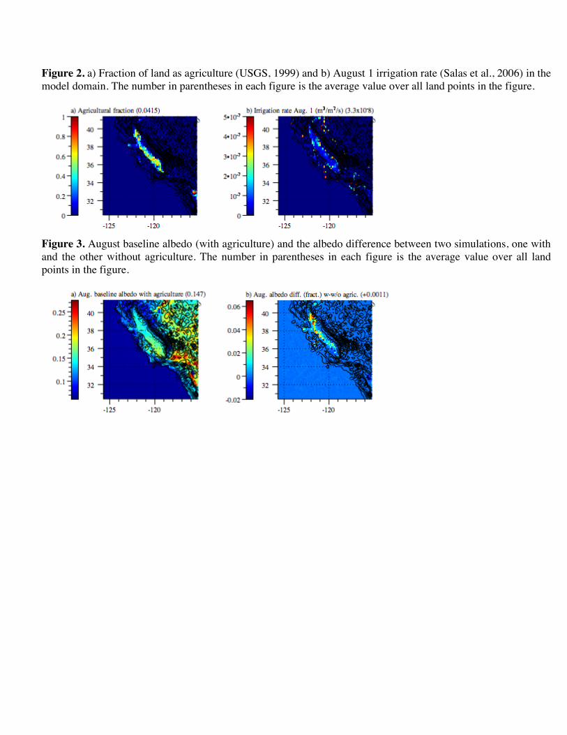
Figure 2. a) Fraction of land as agriculture (USGS, 1999) and b) August 1 irrigation rate (Salas et al., 2006) in the model domain. The number in parentheses in each figure is the average value over all land points in the figure.

Figure 3. August baseline albedo (with agriculture) and the albedo difference between two simulations, one with and the other without agriculture. The number in parentheses in each figure is the average value over all land points in the figure.

Figure 4. Modeled August-averaged baseline values (with irrigation and current albedo of agriculture) (left panel), baseline values minus those without irrigation (w-w/o irrig.) (middle panel), and baseline values minus those without irrigation and with pre-agriculture albedo (w-w/o agric.) (right panel) for several parameters in the California domain. Each number in parentheses is the average value over all land points.

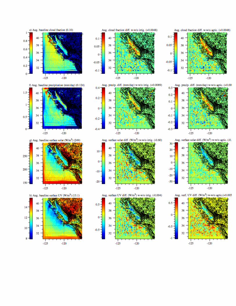
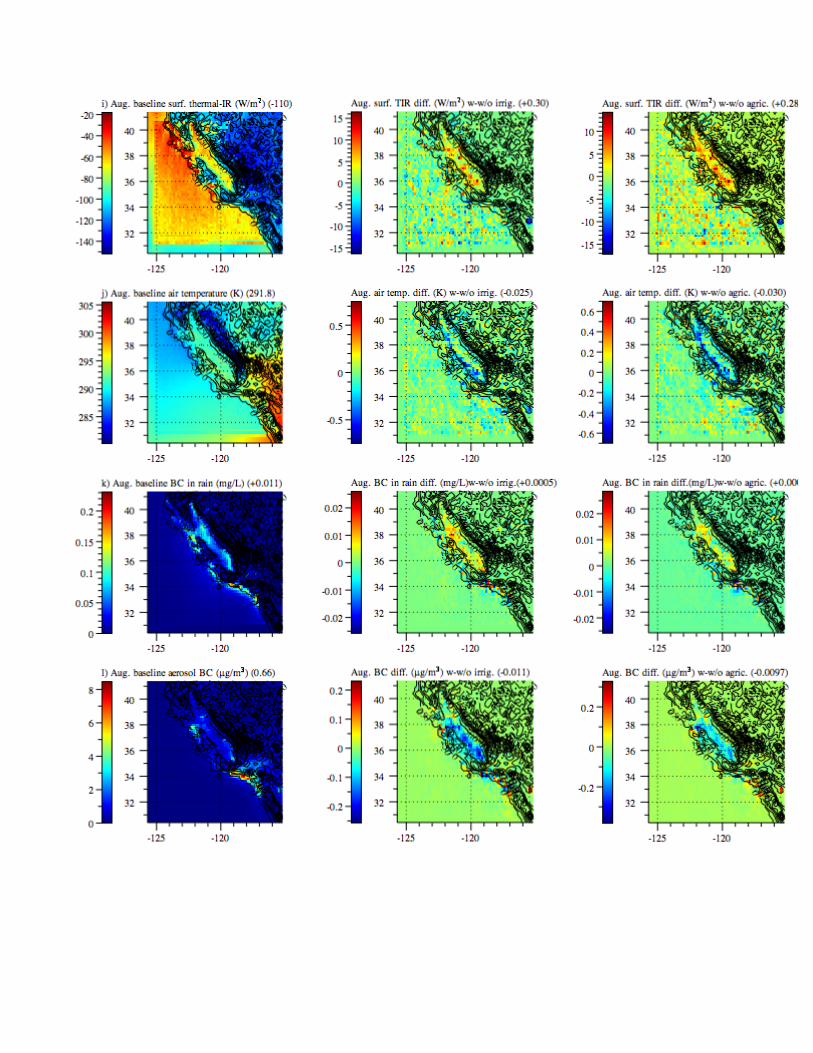
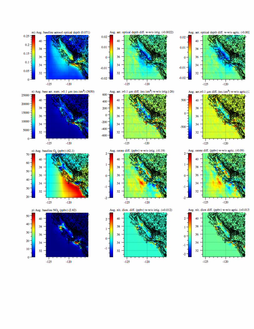
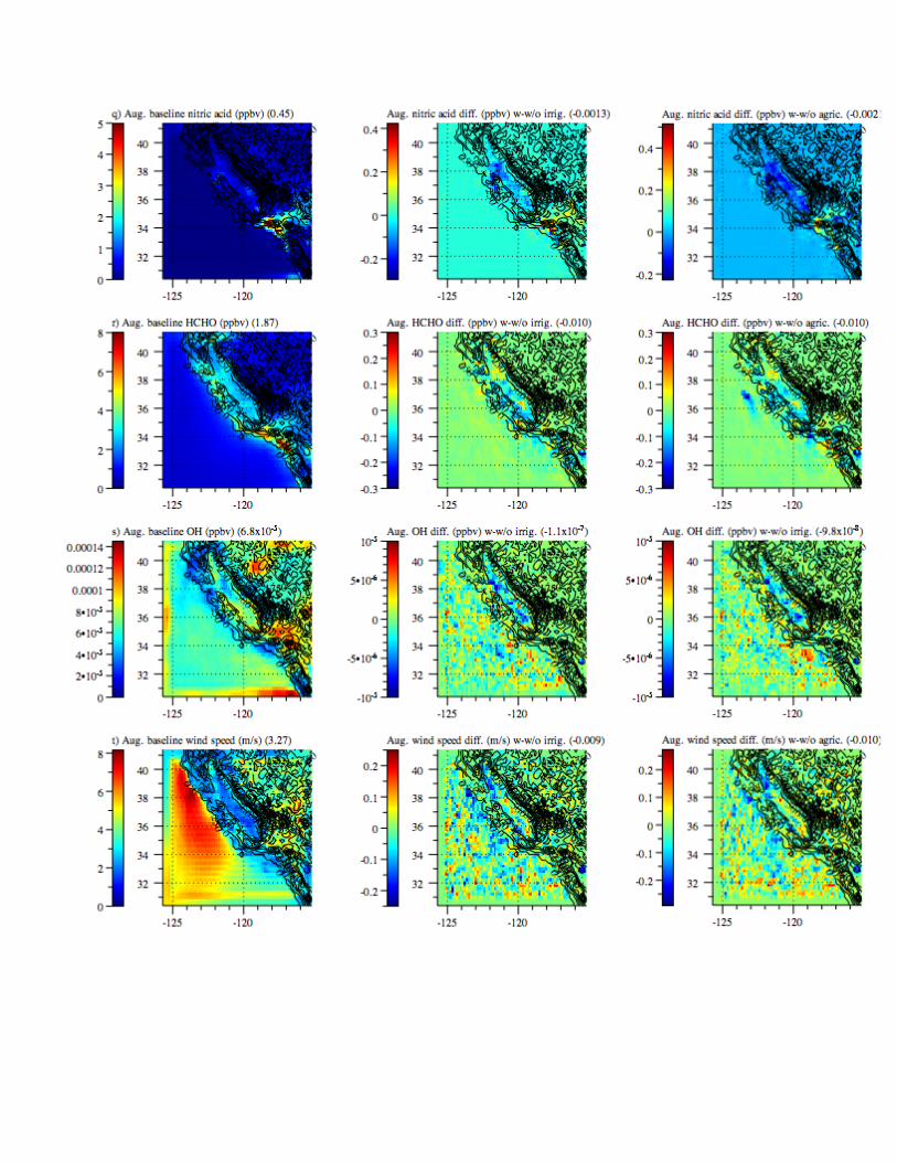
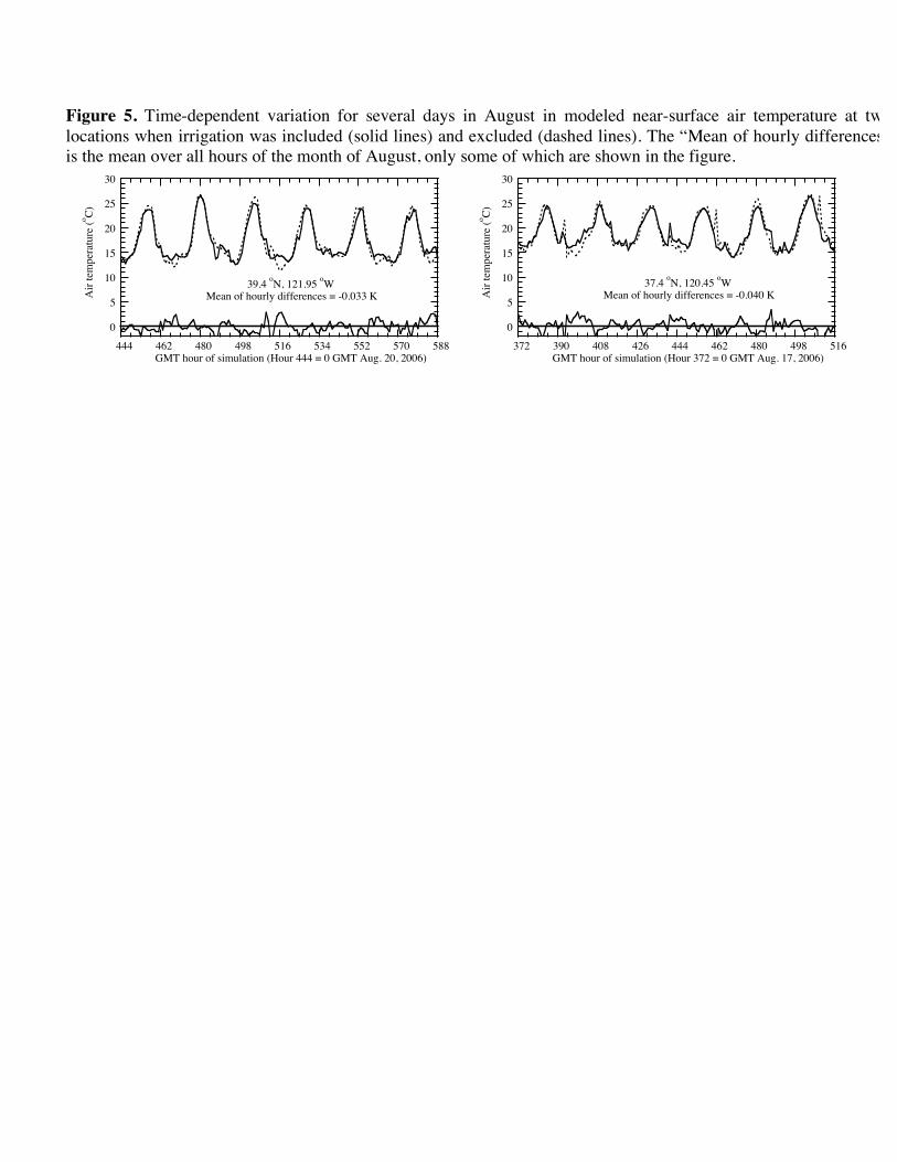
Figure 5. Time-dependent variation for several days in August in modeled near-surface air temperature at two locations when irrigation was included (solid lines) and excluded (dashed lines). The “Mean of hourly differences” is the mean over all hours of the month of August, only some of which are shown in the figure.

0

5

10

15

20

25

30

444 462 480 498 516 534 552 570 588

Air

tem

per

atu

re (

oC

)

GMT hour of simulation (Hour 444 = 0 GMT Aug. 20, 2006)

39.4 oN, 121.95

oW

Mean of hourly differences = -0.033 K

0

5

10

15

20

25

30

372 390 408 426 444 462 480 498 516

Air

tem

per

atu

re (

oC

)

GMT hour of simulation (Hour 372 = 0 GMT Aug. 17, 2006)

37.4 oN, 120.45

oW

Mean of hourly differences = -0.040 K

Figure 6. Modeled versus measured February precipitation.

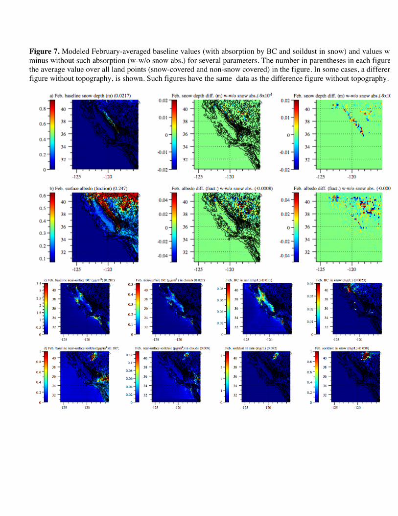
Figure 7. Modeled February-averaged baseline values (with absorption by BC and soildust in snow) and values with minus without such absorption (w-w/o snow abs.) for several parameters. The number in parentheses in each figure is the average value over all land points (snow-covered and non-snow covered) in the figure. In some cases, a difference figure without topography, is shown. Such figures have the same data as the difference figure without topography.