The effects of institutional and technological change and business cycle fluctuations on seasonal patterns in quarterly industrial production series

Econometrics Journal(2003), volume6, pp. 79–98.

The effects of institutional and technological change andbusiness cycle fluctuations on seasonal patterns in quarterly

industrial production series

DICK VAN DIJK†§, BIRGIT STRIKHOLM ‡ AND TIMO TERASVIRTA‡

†Econometric Institute, Erasmus University Rotterdam, P.O. Box 1738, NL-3000 DR Rotterdam,The Netherlands

E-mail:[email protected]‡Department of Economic Statistics, Stockholm School of Economics, Box 6501,

SE-113 83 Stockholm, SwedenE-mail:[email protected]; [email protected]

Received: February 2003

Summary Changes in the seasonal patterns of macroeconomic time series may be dueto the effects of business cycle fluctuations or to technological and institutional change orboth. We examine the relative importance of these two sources of change in seasonality forquarterly industrial production series of the G7 countries using time-varying smooth transitionautoregressive models. We find compelling evidence that the effects of gradual institutionaland technological change are much more important than the effects attributable to the businesscycle.

Keywords: Nonlinear time series, Seasonality, Smooth transition autoregression, Struc-tural change, Time-varying parameter.

1. INTRODUCTION

Seasonal fluctuations are an important source of variation in many macroeconomic time series.When monthly or quarterly series are modelled, it is often assumed that the seasonal patternof the series is constant over time, in which case it may be characterized by seasonal dummyvariables, see Miron (1996) and Miron and Beaulieu (1996), among others. On the other hand,it has been known for a long time that seasonality in a series may change over time. As Kuznets(1932) remarked:

For a number of years statisticians have been concerned with the problem ofmeasuring changes in the seasonal behaviour of time series.

The possible causes for such time-variation in seasonal patterns have also been a longstandingobject of interest. After examining a number of employment series from various countries andregions, Gjermoe (1931) wrote (in Norwegian):

§Corresponding author.

c© Royal Economic Society 2003. Published by Blackwell Publishing Ltd, 9600 Garsington Road, Oxford OX4 2DQ, UK and 350 MainStreet, Malden, MA, 02148, USA.

80 Dick van Dijk et al.

The strength of seasonal fluctuations has to do with thelevelof business activity. Amonth in a year of low employment is more affected by seasonality than the samemonth in a year of high employment (emphasis in original).

In fact, Gjermoe (1926) had already made a similar point.

The possibility that seasonality is affected by the business cycle has been reconsidered in themore recent literature. For example, Canova and Ghysels (1994) and Franses (1996, pp. 86–87)find that the seasonal pattern in quarterly US output growth is affected by the (NBER-dated)business cycle. In particular, it is found that the summer slowdown is less pronounced aroundbusiness cycle peaks. A similar conclusion is reached by Cecchetti and Kashyap (1996) andMatas-Mir and Osborn (2001), using an international data set of monthly production series at theindustry-level. Cecchettiet al. (1997) and Krane and Wascher (1999) document the same effectof the business cycle on seasonal patterns in US production, inventories and employment, whichis attributed to the fact that during a boom the presence of capacity constraints forces firms toproduce a larger fraction of output in off-peak seasons.

Business cycle fluctuations are not the only possible reason for changes in the seasonalpattern of output or employment series. In particular, technological change and changes ininstitutions and habits may cause changes in seasonality as well. As an example of the former,in the construction industry it has become possible to keep a construction site going year-roundin countries where, a few decades ago, work was interrupted for the winter months. As to thelatter type of change, the increase in paid leisure over the last few decades has gradually changedpeople’s vacation habits. At least in some Scandinavian countries it has become customary tospend a week of the annual holiday in the winter. Yet another example may be the increasinglyefficient use of capital and just-in-time production techniques. Many factories in Europe nolonger close down for the summer vacation but keep the production process running withoutinterruption. In all these examples, the result may have been that the seasonal pattern of, forexample, output and consumption series has changed over time.

Our aim is to compare the effects on seasonality of gradual institutional and technologicalchange with the effects attributable to the business cycle. As for the former, there do not seemto exist reliable aggregate measures for these changes. We allow for the possibility that theaggregate change is steady and continuous and simply use time as a proxy variable for it. Thismeans that we in fact contrast ‘Kuznets-type’ unspecified changes in seasonality with ‘Gjermoe-type’ changes caused by fluctuations in economic activity. The main question we ask is: whichof the two types is more prominent in practice, if any? We shall investigate the problem usingquarterly industrial production series of the world’s leading market economies, the G7 countries.

In this work, the logarithmic time series are differenced once in order to achieve stationarity,and the differenced series are used for modelling. For most countries, these first differences, orquarterly growth rates, are dominated by seasonal variation that almost completely inundates theother features of the series, see Figures 2 and 3 in what follows. The models we are going tobuild are constructed strictly to investigate the main research question formulated above aboutreasons for time-variation in seasonal patterns of industrial production series. Because mostof the variation captured by the parameters will be seasonal variation, models based on firstdifferences are not likely to be appropriate tools in forecasting industrial production severalquarters ahead. A typical forecaster would rather begin his analysis by transforming the originalquarterly series into annual differences which emphasize the low-frequency variation he is mostlikely interested in, build a linear or nonlinear model for them and use that for forecasting.

c© Royal Economic Society 2003

Sources of change in seasonality in industrial production 81

The plan of the paper is as follows. In Section 2, we describe the output series for the G7countries, focusing on the properties of their seasonal cycles. In Section 3, we present ourmain statistical tool, the time-varying smooth transition autoregressive (TV-STAR) model. InSection 4, we use Lagrange multiplier (LM) tests derived from the TV-STAR framework foraddressing the question of whether the changes in the seasonal patterns in the output series aredue to the effects of business cycle fluctuations or to technological and institutional change orboth. For all series except the US, we find convincing evidence that ‘Kuznets-type’ unspecifiedchange is much more important than ‘Gjermoe-type’ business cycle-induced change. In contrastto previous research our analysis suggests that, for the US, seasonality does not vary over thebusiness cycle nor has it changed over time. In Section 5, we specify and estimate TV-STARmodels to gain further insight into when and how seasonality in the quarterly output series haschanged. Section 6 contains final remarks. Material that for space reasons has been omitted fromthe paper is available at the websitehttp://swopec.hhs.se/hastef/abs/hastef429.htm.

2. PRELIMINARIES

2.1. Data

Our data set consists of quarterly seasonally unadjusted industrial production volume indexesfor the G7 countries, taken from the OECDMain Economic Indicators. The sample period runsfrom 1960.1 until 2001.3, except for Canada for which the series is available only from 1961.1.Obvious outliers in 1963.1 and 1968.2 for France and in 1969.4 for Italy are replaced by theaverage of the index values in the same quarter of the previous and the following year.

Seasonal variation is a dominant component in the German and the UK series, and the same istrue for France, Italy and Canada. A regression of the quarterly growth rates on the four seasonaldummies confirms this: the coefficients of determination lie between 0.68 (Canada) and 0.92(France). They are lower for Japan(0.21) and the US (only 0.06).

A common feature for Canada and three European countries, Germany, France and the UK, isthat the seasonal variation in the industrial output series appears to have dampened over time; seealso Figure 1. In particular, the drop in output in the third and fourth quarters peak have becomeless pronounced, which was also documented by Canova and Hansen (1995). The Japanese andthe US series do not show a third-quarter summer holiday slack in production. In the US, thequarterly growth in the 1990s was actually highest in the third quarter and lowest in the fourthquarter.

2.2. Deterministic and stochastic seasonality

In the case of nonstationary time series, time-varying seasonal patterns may often be convenientlycharacterized by seasonal unit roots, see Hylleberg (1994). Autoregressive models of seasonallydifferenced data are capable of generating series in which the seasonal pattern evolves overtime. In realizations from such models ‘summer may become winter’ or, in general, seasonsmay gradually ‘trade places’. Structural time series models offer another way of modellingstochastically time-varying seasonality; see Harvey (1989, Ch. 6) and Harvey and Scott (1994).In this approach, the time series is divided into components, of which the seasonal one isrepresented by a linear combination of trigonometric functions with stochastic coefficients. Ifthese coefficients have zero variance, seasonality is deterministic.



Figure 1. Industrial production for Germany, Japan and the UK.

Neither one of these alternatives, seasonal differencing or decomposing the time series,is directly applicable to our situation. The reason is that we intend to consider two types oftime-varying seasonality, variation due to technological and institutional change (‘unspecifiedchange’) and variation induced by cyclical fluctuations in economic activity, simultaneously. Thisrequires a model within which we can distinguish these two different sources of variation on theseasonal pattern from each other and thus compare their relative importance. For this reason we



employ the TV-STAR model of Lundberghet al. (2003), to be discussed in the next section,for our investigation. The paper that comes closest to ours as far as the modelling approach isconcerned is Matas-Mir and Osborn (2001). These authors use a threshold autoregressive modelin which the seasonal pattern, characterized by seasonal dummy variables, switches according toa business cycle indicator. Structural changes in seasonality are also accounted for by allowinglinear trends in the coefficients of the seasonal dummy variables. An important aspect in whichour approach differs from the one in Matas-Mir and Osborn (2001) is that the TV-STAR modelallows for more flexible nonlinear trends in seasonality, as will become clear in the following.

3. THE TV-STAR MODEL

We use the TV-STAR model to investigate the source of changes in seasonality in the G7 outputseries, because it is capable of describing business cycle nonlinearity and structural change inthe characteristics of a time series variable simultaneously. To suit our purposes, we augment themodel by seasonal dummies, such that for our quarterly time series it has the following form:

1yt = [(φ′

1xt + δ′

1Dt )(1 − G1(wt )) + (φ′

2xt + δ′

2Dt )G1(wt )][1 − G2(t∗)]

+ [(φ′

3xt + δ′

3Dt )(1 − G1(wt )) + (φ′

4xt + δ′

4Dt )G1(wt )]G2(t∗) + εt , (1)

whereyt is the log-level of the industrial production index,wt a stochastic transition variable,1

denotes the first differencing operator, defined by1kyt ≡ yt − yt−k for all k 6= 0 and1 ≡ 11,xt = (1, x′

t )′, xt = (1yt−1, . . . ,1yt−p)

′, Dt = (D∗

1,t , D∗

2,t , D∗

3,t )′

≡ (D1,t − D4,t , D2,t −

D4,t , D3,t − D4,t )′, Ds,t , s = 1, . . . , 4 are seasonal dummy variables, withDs,t = 1 when time

t corresponds with seasons andDs,t = 0 otherwise, andt∗ ≡ t/T with T denoting the samplesize. The transition functionsG j (st ) ≡ G j (st ; γ j , c j ), j = 1, 2, are assumed to be given by thelogistic function

G j (st ; γ j , c j ) = (1 + exp{−γ j (st − c j )/σst })−1, γ j > 0, (2)

where the transition variablest = wt ( j = 1) or st = t∗ ( j = 2), andσst = [var(st )]1/2

makesγ j scale-free. Asst increases, the logistic function changes monotonically from 0 to 1,with the change being symmetric around the location parameterc j , asG j (c j − z; γ j , c j ) =

1 − G j (c j + z; γ j , c j ) for all z. The slope parameterγ j determines the smoothness of thechange in the value of the logistic function. Asγ j → ∞, the logistic functionG j (st ; γ j , c j )

approaches the indicator functionI [st > c j ] and, consequently, the change ofG j (st ; γ j , c j )

from 0 to 1 becomes instantaneous atst = c j . Whenγ j → 0, G j (st ; γ j , c j ) → 0.5 for allvalues ofst .

The TV-STAR model distinguishes four regimes corresponding with combinations ofG1(wt )

andG2(t∗) being equal to 0 or 1. The transition variablewt in (1) is assumed to be a laggedseasonal difference,wt = 14yt−d, for certaind > 0. As this variable tracks the businesscycle quite closely for our quarterly industrial production series (see panels (b), (d) and (f) ofFigure 1), and because the logistic functionG j (st ) is a monotonic transformation ofst , theregimes associated withG1(14yt−d) = 0 and 1 will roughly correspond with recessions andexpansions, respectively. Thus, using14yt−d as transition variable ensures that the TV-STAR



model allows for ‘Gjermoe-type’ change in the seasonal pattern ofyt .1 On the other hand, thefunctionG2(t∗) enables the model to describe ‘Kuznets-type’ unspecified change as well.

The reason for defining the elements ofDt as D∗s,t ≡ Ds,t − D4,t , s = 1, 2, 3, is that

it effectively separates the deterministic seasonal fluctuations from the overall intercept. Forexample, the coefficients inδ1 = (δ11, δ12, δ13)

′ measure the difference between the interceptin the first three quarters of the year and the overall intercept, given by the first element ofφ1,in the regimeG1(14yt−d) = 0 andG2(t∗) = 0. The difference for the fourth quarterδ14 isobtained asδ14 = −

∑3s=1 δ1s. This parameterization makes it easy, for example, to test constant

seasonality while allowing for a business cycle influenced intercept under the null hypothesis, cf.Franses (1996, pp. 86–87).

The general TV-STAR model in (1) allows both the dynamics and the seasonal properties ofthe growth rate of industrial production to vary both over the business cycle and over time.By imposing appropriate restrictions on either the autoregressive parameters or the seasonaldummy parameters or on both, more restrictive models can be obtained. Of particular interesthere are models in which seasonality only varies either over time or over the business cycle. Amodel in which seasonality is constant over time is obtained ifδ1 = δ3 andδ2 = δ4 in (1).Similarly, a model in which seasonality is constant over the business cycle is obtained by settingδ1 = δ2 and δ3 = δ4. Whenδ1 = δ2 = δ3 = δ4, seasonality is linear and constant overtime. Imposing analogous restrictions onφi , i = 1, . . . , 4 results in models with constant butnonlinear, linear but time-varying, and linear and constant autoregressive dynamics, respectively.If both the seasonal patterns and the autoregressive dynamic structure are constant either overtime or over the business cycle, the TV-STAR model reduces to a STAR or TV-AR model,respectively. All these restrictions are testable, as will be discussed in the next section. Oftena useful restricted TV-STAR model is an additive one, containing a nonlinear and a time-varyingcomponent. For example, a model in which the seasonal dummy coefficients vary over time andthe autoregressive parameters enter nonlinearly can be written as

1yt = φ∗′

1 xt + δ∗′

1 Dt + φ∗′

2 xt G1(wt ) + δ∗′

2 Dt G2(t∗) + εt . (3)

In Section 5 we will use this form for the models for the industrial production series.

On the other hand, the TV-STAR model (1) is restrictive in the sense that it requires anynonlinearity or structural change to be common across the autoregressive dynamics and seasonaldummies. But then, model (3) does not contain that restriction becauseG1 only controls thelag structure andG2 the seasonal component. A potential limitation of both models (1) and(3) is that they only allow for a single change in the seasonal pattern over time. The modelcan be generalized in a straightforward fashion to accommodate multiple changes by includingadditional time-varying components. For example, an additive model in which the autoregressiveparameters enter nonlinearly and the seasonal dummy coefficients change over time following amixture of two patterns is given by

1yt = φ∗′

1 xt + δ∗′

1 Dt + φ∗′

2 xt G1(wt ) + δ∗′

2 Dt G2(t∗) + δ∗′

3 Dt G3(t∗) + εt . (4)

1It may be argued, however, that GNP is a more representative and more commonly used indicator of the business cyclethan industrial production. In fact, we repeated our tests described in Section 4 using lagged seasonal differences of GNPinstead of14yt−d as the transition variable. The results were very similar to the ones obtained by using14yt−d andtherefore are omitted.



4. CHANGES IN THE SEASONAL PATTERN AND THEIR CAUSES

4.1. Testing linearity and parameter constancy in the TV-STAR framework

The question posed in the Introduction about the causes of fluctuations in the seasonal pattern isaddressed within the framework of the TV-STAR model (1), in particular by testing hypothesesabout the coefficients of the model. In the previous section, it was emphasized that linearityor parameter constancy in the TV-STAR model (1) may be achieved by imposing equalityrestrictions on certain coefficient vectorsδi and/orφi . Note, however, that linearity or parameterconstancy of both the seasonal pattern and the dynamic autoregressive structure also results ifthe smoothness parameterγ j in the corresponding transition functionG j is set equal to zero.This is an indication of an identification problem present in the model: the TV-STAR model isonly identified under the alternative, not under the null hypothesis. For a general discussion, seeHansen (1996). In this paper, we follow the approach of Lundberghet al.(2003) and circumventthe identification problem by approximating the transition functions by their first-order Taylorexpansions, see also Luukkonenet al. (1988).

Let the null hypothesis of interest beH0 : γ1 = γ2 = 0, which is to be tested againstthe alternative hypothesisH1 : γ1 > 0 and/orγ2 > 0. Under H0, model (1) reduces toa seasonality-augmented linear autoregressive model, which we assume to be stationary andergodic. Furthermore, we assume that the moment conditionE[(1yt )

2(14yt )2] < ∞ is satisfied,

which is necessary for the asymptotic inference to be valid. In testingH0, we only assume thatd ∈ {1, . . . , r } in (1), that is, the true delayd is unknown but assumed to be no greater thanr . A convenient way to parameterize this assumption is by settingwt =

∑ri =1 ai 14yt−i , with

ad = 1 andai = 0 for all i 6= d; see Luukkonenet al. (1988) for further details. In this case,after rearranging terms the first-order Taylor expansion of (1) aroundH0 becomes

1yt = φ∗′

1 xt + δ∗′

1 Dt +

r∑i =1

(φ∗′

2,i xt + δ∗′

2,i Dt )14yt−i + (φ∗′

3 xt + δ∗′

3 Dt )t∗

+

r∑i =1

(φ∗′

4,i xt + δ∗′

4,i Dt )t∗14yt−i + R(γ1, γ2) + εt , (5)

whereR(γ1, γ2) is a remainder from the two Taylor expansions. Under the null hypothesis oflinearity and parameter constancy,R(γ1, γ2) ≡ 0, such that this remainder does not affect thedistribution theory.

Equation (5) is linear in parameters. Furthermore, and this is crucial, the parameter vectorsφ∗

2 = (φ∗′

2,1, . . . ,φ∗′

2,r )′

= γ1φ∗

2(θ) and δ∗

2 = (δ∗′

2,1, . . . , δ∗′

2,r )′

= γ1δ∗

2(θ), φ∗

3 = γ2φ∗

3(θ)

and δ∗

3 = γ2δ∗

3(θ), andφ∗

4 = (φ∗′

4,1, . . . ,φ∗′

4,r )′

= γ1γ2φ∗

4(θ) and δ∗

4 = (δ∗′

4,1, . . . , δ∗′

4,r )′

=

γ1γ2δ∗

4(θ) where φ∗

j (θ), δ∗

j (θ), j = 2, 3, 4, are non-zero functions of the parametersθ =

(φ′

1, . . . ,φ′

4, δ′

1, . . . , δ′

4)′. In view of this, the original null hypothesis becomes

H′

0 : φ∗

2,i = φ∗

3 = φ∗

4,i = 0, δ∗

2,i = δ∗

3 = δ∗

4,i = 0, i = 1, . . . , r

in the transformed equation (5). The standard LM statistic for testingH′

0 has an asymptoticχ2

distribution with(p + 4)(1 + 2r ) degrees of freedom under the null hypothesis. In practice, anF-version of the test is recommended because its size properties in small and moderate samples



are much better than those of theχ2-based test statistic, especially when the number of param-eters tested becomes large relative to the sample size. It should be noted that, depending on thevalues ofp andr , certain termsφ∗

2,i,014yt−i andφ∗

2,i, j 1yt− j 14yt−i should be excluded from(5) to avoid perfect multicollinearity.

In order to keep the notation simple, we have so far discussed the case where the standardlogistic function (2) is the transition function. It is useful to generalize this slightly as follows.Let

G j (st ; γ j , c j ) =

(1 + exp

{−

γ j

σ kst

k∏i =1

(st − c j i )

})−1

, γ > 0, c j 1 ≤ · · · ≤ c jk . (6)

This function allows more flexibility in the transition. When we test linearity against the TV-STAR model (1) with (6), a first-order Taylor expansion of (6) leads to terms with higherpowers of14yt− j and t∗ in equation (5); see, for example, Luukkonenet al. (1988), Grangerand Terasvirta (1993, Ch. 6) or Lundberghet al. (2003). The dimension of the null hypothesisincreases linearly ink, which implies that for small sample sizes such as the one available here,the tests fork > 1 can only be computed for fairly small values ofp andr . In the following wereport results fork = 1 and, whenever possible, fork = 3. Test results fork = 2 are availableupon request. The corresponding statistics are denoted as LMk.

Finally, it should be pointed out that the lag lengthp in (1) is unknown. It is selected fromthe linear seasonality-augmented autoregressive model using BIC with the maximum order setequal topmax = 12. As remaining residual autocorrelation may be mistaken for nonlinearity, weapply the Breusch–Godfrey LM test to examine the joint significance of the first 12 residualautocorrelations in the model that is preferred by the BIC. If necessary, the lag lengthp isincreased until the null hypothesis of no error autocorrelation can no longer be rejected at the5% significance level. Testing is carried out conditionally on the selected lag lengthp.

4.2. Testing hypotheses of interest

The test just described is a general linearity test within our maintained TV-STAR model (1). Inthis paper, however, the main interest lies in testing subhypotheses that place restrictions on theseasonal dummy variables. We may also set certain parameter vectors to zero (null vectors)a priori. This leads to a maintained model that is a submodel of (1). In particular, we areinterested in testing constant seasonality against the alternative that the seasonal pattern changessmoothly over time, conditional on the assumption that seasonality is not affected by the businesscycle and that the autoregressive structure does not change. In terms of the parameters in (5), thecorresponding null hypothesis is

HTV−AR,Ds,t0 : δ∗

3 = 0 assumingφ∗

2,i = φ∗

3 = φ∗

4,i = 0, δ∗

2,i = δ∗

4,i = 0, i = 1, . . . , r.

Another hypothesis of interest is testing constant seasonality against the alternative that theseasonal pattern is affected by the business cycle only:

HSTAR,Ds,t0 : δ∗

2,i = 0 assumingφ∗

2,i = φ∗

3 = φ∗

4,i = 0, δ∗

3 = δ∗

4,i = 0, i = 1, . . . , r.

A test against the joint alternative of smooth change and fluctuations ascribed to the businesscycle may be formed accordingly. The corresponding null hypothesis is denoted as

HTV−STAR,Ds,t0 .



These tests are based on the assumption of linearity of the dynamic structure of the time series1yt . But then, the first difference of the volume of industrial production may be a nonlinear ortime-varying process. One way of accounting for this possibility is to relax the zero restrictionsonφ∗

2,i , φ∗

3 andφ∗

4,i in the above tests. While testing the resulting null hypotheses is not difficultin practice, this may not be an optimal way to proceed. Instead it may be better to test ourtwo competing hypotheses concerning seasonality within a model which explicitly models thechanges in the autoregressive structure, either as a function of time (TV-AR) or as a functionof the business cycle (STAR). In that case, we may begin by testing linearity against STAR andTV-AR. The relevant null hypotheses (assuming constant seasonality and unknown delayd) are

HSTAR,1yt− j0 : φ∗

2,i = 0 assumingφ∗

3 = φ∗

4,i = 0, δ∗

2,i = δ∗

3 = δ∗

4,i = 0, i = 1, . . . , r,

and

HTV−AR,1yt− j0 : φ∗

3 = 0 assumingφ∗

2,i = φ∗

4,i = 0, δ∗

2,i = δ∗

3 = δ∗

4,i = 0, i = 1, . . . , r,

respectively. Assume for a moment thatHSTAR,1yt− j0 is rejected andH

TV−AR,1yt− j0 is not. This

implies that the dynamic behaviour of the process, excluding seasonality, may be adequatelycharacterized by a STAR model. We subsequently specify, estimate and evaluate a STAR modelfor 1yt . The issue is now the constancy of the coefficients of the seasonal dummy variables inthe STAR model. The maintained model may be written as follows:

1yt = φ′

1xt + φ′

2xt G1(st ) + {δ1 + δ2G2(14yt−l ) + δ3G3(t∗)

+ δ4G2(14yt−l )G3(t∗)}′Dt + εt , (7)

where the transition functionsG2(14yt−l ), l > 0, andG3(t∗) are logistic functions as in (6).Note that we can choose eitherst = 14yt−d or st = t∗ in (7). The relevant parameter constancyhypotheses can now be formulated within equation (7) in terms of the slope parameters in thetransition functionsG2(14yt−l ), l > 0 andG3(t∗) or in terms of the coefficient vectorsδ2,δ3 and δ4. Asymptotic theory for inference requires the assumption that the null model, (7)with δ2 = δ3 = δ4 = 0, is stationary and ergodic. Testing is based on the first-order Taylorapproximation ofG2(14yt−l ) andG3(t∗) as described in Section 4.1; for a general account ofSTAR model misspecification tests, see, for example, Terasvirta (1998) or van Dijket al.(2002).

4.3. Results

Table 1 reportsP-values of theF-statistics for testingHTV−AR,·0 , HSTAR,·

0 andHTV−STAR,·0 based

on a linear null model. The column headings LM1 and LM3 correspond to tests based on thefirst-order Taylor expansion of the transition function (6) withk = 1 and 3, respectively. Therow headingsDs,t and1yt− j correspond to tests involving the seasonal pattern only and theautoregressive coefficients only, respectively.2 All tests are computed with the maximum valueof the unknown delayr set equal to 4.

Plenty of evidence is found to support the argument that seasonality is changing forunspecified reasons, including institutional and technological change and actions by the statistics

2To save space, results for tests on the seasonal pattern and the autoregressive structure simultaneously are omitted butare available at the website.



Table 1.Testing linearity and parameter constancy of quarterly growth rates in industrial production.

Parameters STAR TV-AR TV-STAR

tested LM1 LM3 LM1 LM3 LM1 LM3

Canada (p = 8)

Ds,t 0.21 0.72 0.28 5.9E−5 0.20 0.049

1yt− j 0.068 0.35 0.37 0.11 0.13 —

France (p = 8)

Ds,t 0.34 0.035 1.0E−5 3.6E−8 3.8E−3 0.012

1yt− j 0.062 0.12 4.9E−5 5.7E−5 0.033 —

Germany (p = 5)

Ds,t 0.11 0.51 0.012 2.4E−4 0.16 0.10

1yt− j 3.8E−3 8.3E−3 0.015 0.086 0.028 0.070

Italy ( p = 6)

Ds,t 0.17 0.21 0.061 9.7E−6 0.29 0.11

1yt− j 0.094 0.12 0.11 8.9E−5 0.24 0.26

Japan (p = 5)

Ds,t 0.066 8.2E−4 0.019 2.5E−5 2.2E−4 5.1E−3

1yt− j 0.024 8.1E−3 3.7E−3 1.2E−3 1.1E−3 0.039

United Kingdom (p = 9)

Ds,t 0.030 0.071 2.1E−3 2.1E−3 0.016 2.1E−4

1yt− j 0.039 0.075 5.1E−3 0.016 0.058 —

United States (p = 7)

Ds,t 0.034 0.11 0.020 0.016 0.089 0.38

1yt− j 6.4E−3 0.014 0.49 0.73 0.33 —

Notes: The table containsP-values ofF-variants of the LMk, k = 1, 3, tests of linearity and parameter constancy withinthe TV-STAR model (1) for quarterly industrial production growth rates. The delay parameterd is assumed unknown,that iswt =

∑ri =1 ai 14yt−i with ad = 1 andai = 0 for all i 6= d, wherer is set equal to 4. The null hypotheses of

the different tests are linearity conditional on parameter constancy (STAR), constancy conditional on linearity (TV-AR)and linearity and constancy (TV-STAR). Rows labelledDs,t and1yt− j contain results for testing the seasonal dummiesand the lagged growth rates, respectively. All tests are performed conditional on assuming that the remaining parametersenter linearly and with constant parameters. A dash indicates that the test could not be computed due to a shortage indegrees of freedom.

producer, proxied by the time variable. The results for the LM1 statistic are mixed, but LM3rejects the null hypothesisHTV−AR,Ds,t

0 at the 0.01 level for all series except the US. On the otherhand, there is much less evidence to support the notion that seasonality varies with the business

cycle, as theP-values for the tests corresponding toHSTAR,Ds,t0 are considerably larger for all

seven countries. The only occasion in which aP-value lies below 0.01 is LM3 for Japan. ForJapan, there is in fact substantial evidence of both nonlinearity and parameter nonconstancy in theseries. For the other six countries, it seems that business cycle fluctuations are not a major causeof changes in the seasonal pattern. Finally, another fact obvious from Table 1 worth mentioning



is that testing against both types of changes in seasonality jointly has an adverse effect on power.More information is gained by looking at the two alternatives separately.

Two objections may be made at this point. First, seasonality may not be fully explainedby the seasonal dummy variables, but part of the seasonal variation may be absorbed in (orexplained through) the autoregressive dynamic structure of model (1). Pierce (1978) discussedthis possibility in connection with seasonal adjustment of economic time series. This variationmay be related to the business cycle. Second, results on testing linearity against STAR in Table 1(cells (1yt− j , STAR)), suggest that the dynamic behaviour of some of the industrial productionseries may be nonlinear. For other series a case can be made for a TV-AR process, that is, thedynamic behaviour may be time-varying because of phenomena proxied by time. It may thereforebe argued that the results just presented are affected by misspecification of the null model andthat in order to avoid this, it should already accommodate non-seasonal nonlinearity.3

This possibility can be considered by first modelling nonseasonal nonlinearity and carryingout the tests of constancy of the seasonal parameters within the nonlinear model, as discussed inSection 4.2. Detailed results of this approach are omitted and can be found at the website. Theycan be summed up by saying that by and large, the previous pattern is repeated. Admittedly, theP-values are somewhat higher because the autoregressive structure now explains more variationin these series than before. In fact, allowing for time-varying or STAR-type dynamic structuresonly eliminates the ‘Kuznets-type’ change in the seasonal pattern in the UK and the US. Theseasonal component in the US industrial production is very small anyway. There is weak evidencethat it may have been changing with the business cycle: theP-value for LM1 when testing againstSTAR equals 0.064 (see the website).

A general conclusion arising from the complete set of test results is that the institutional,technological and other (due to statistics producers) changes proxied by time are the main causeof changes in the seasonal pattern in the output series of G7 countries. As we have just pointedout, however, our conclusions are not completely unaffected by the choice of the model used forcarrying out the relevant tests. This may not be surprising, and mentioning it may even soundtrivial. Nevertheless, we wish to argue that our general conclusion seems remarkably robust tothe choice of the null model.

5. MODELLING CHANGING SEASONAL PATTERNS BY TV-STAR MODELS

Our test results in the previous section clearly show that seasonal patterns in the G7 output seriesare not constant over time. In this section, our aim is to characterize this change with a parametricmodel, instead of just demonstrating its existence through a number of hypothesis tests. We willattempt to build an adequate TV-STAR model for each of the series and focus on the componentsrelated to seasonal variation.

As the TV-STAR model is a rather flexible nonlinear model, we need a coherent modellingstrategy or modelling cycle in order to arrive at an acceptable parameterization. We choose the‘specific-to-general’ strategy of Lundberghet al. (2003). The main features of this modellingcycle are the following. First, starting with a seasonality-augmented linear autoregressive model,test linearity against STAR (14yt−d being the transition variable, where the value ofd is varied

3An alternative modification of the tests presented in Table 1 would be to allow the overall intercept to be affected by thebusiness cycle when testing for ‘Gjermoe’-type changes in seasonality, and to allow for the intercept to be time-varyingwhen testing for ‘Kuznets’-type changes in seasonality, cf. Franses (1996, pp. 86–87). Results from these tests are verysimilar to the ones shown in Table 1 and are therefore omitted.



to determine the appropriate value of the delay parameter) and TV-AR (t∗ being the transitionvariable). Choose the submodel against which the rejection is strongest (if it is strong enough,otherwise accept the linear model). Estimate the chosen model; this involves repeated estimationwhile reducing the size of the model through imposing exclusion and equality restrictions onparameters. Evaluate the estimated model by subjecting it to a number of misspecification tests.The results may either indicate that the estimated model is adequate or they may point at thenecessity of extending the model further, for example towards a full TV-STAR model. A detailedaccount of the modelling strategy can be found in Lundberghet al. (2003). Below, we report theTV-STAR models obtained for Germany, Japan and the UK in detail. This is followed by a briefsummary of the results obtained for the remaining countries.

5.1. Germany

For Germany, the results from the LM-type misspecification tests in the linear model indicate thatthe seasonal dummy coefficients may be varying for unspecified reasons and the autoregressivedynamics may be varying with the business cycle. The evidence for the latter disappears,however, once we allow the seasonal dummies to vary over time. To capture the variation in theseasonal pattern, we find that three TV components with standard logistic functions are required.The final specification is:

1yt = 1.67(0.40)

− 8.95(1.13)

D∗1,t + 7.02

(1.04)D∗

2,t − 8.25(1.11)

D∗3,t + 0.16

(0.063)1yt−1 + 0.12

(0.055)1yt−2 − 0.13

(0.062)1yt−7

− 0.18(0.064)

1yt−8 + (− 1.32(0.43)

+ 1.97(0.87)

D∗1,t − 2.56

(1.14)D∗

2,t − 6.26(1.69)

D∗3,t ) × G1(t∗; γ1, c1)

+ (− 6.24(0.94)

D∗2,t + 12.0

(1.24)D∗

3,t ) × G2(t∗; γ2, c2) + ( 4.52(1.28)

D∗2,t + 1.98

(0.94)D∗

3,t ) × G3(t∗; γ3, c3) + εt , (8)

G1(t∗; γ1, c1) = (1 + exp{− 5.89(2.94)

(t∗ − 0.20(0.025)

)/σt∗ })−1, (9)

G2(t∗; γ2, c2) = (1 + exp{− 500(−)

(t∗ − 0.40(−)

)/σt∗ })−1, (10)

G3(t∗; γ3, c3) = (1 + exp{− 5.58(−)

(t∗ − 0.83(0.035)

)/σt∗ })−1, (11)

σε = 1.60, σTV-STAR/AR = 0.70, SK = −0.43(0.015), EK = 0.77(0.026), JB = 8.55(0.014),

LMSC(1) = 0.38(0.54), LMSC(4) = 0.37(0.83), LMSC(12) = 1.17(0.31), ARCH(1) = 8.04(4.5E−3),

ARCH(4) = 8.66(0.070), AICTV-STAR/AR = −0.51, BICTV-STAR/AR = −0.22,

where OLS standard errors are given in parentheses below the parameter estimates,εt denotes theregression residual at timet , σε is the residual standard deviation,σTV-STAR/AR is the ratio of theresidual standard deviations in the estimated TV-STAR model (8) and the best fitting subset ARmodel, SK is skewness, EK excess kurtosis, JB the Jarque–Bera test of normality of the residuals,LMSC( j ) is the LM test for no residual autocorrelation up to and including lagj , ARCH(q) is theLM test of no ARCH effects up to orderq, and AICTV-STAR/AR and BICTV-STAR/AR are differencesbetween the Akaike and Schwarz Information Criteria, respectively, of the estimated TV-STARand the AR models. The numbers in parentheses following the test statistics areP-values. Furthermisspecification tests are reported in the top panel of Table 2. These indicate that the model is



Table 2.Diagnostic tests of parameter constancy and no remaining nonlinearity in TV-STAR models.

Transition Ds,t 1yt− j σ2ε

variable LM1 LM3 LM1 LM3 LM1 LM3

Germany

t 0.91 0.83 0.61 0.49 0.61 0.52

14yt−1 0.54 0.24 0.22 0.16 0.091 0.40

14yt−2 0.29 0.11 0.89 0.63 0.28 0.75

14yt−3 0.70 0.90 0.83 0.62 0.37 0.62

14yt−4 0.41 0.60 0.40 0.51 0.14 0.44

Japan

t 0.34 0.047 0.87 0.35 0.68 0.65

14yt−1 0.21 0.085 0.49 0.21 0.28 0.41

14yt−2 0.35 0.58 0.73 0.31 0.89 0.99

14yt−3 0.59 0.44 0.87 0.95 0.41 0.83

14yt−4 0.56 0.78 0.70 0.95 0.14 0.52

United Kingdom

t 0.21 0.087 0.65 0.36 0.47 0.13

14yt−1 0.46 0.54 0.89 0.22 0.57 0.51

14yt−2 0.92 0.35 0.50 0.89 0.81 0.96

14yt−3 0.69 0.44 0.21 0.26 0.40 0.87

14yt−4 0.62 0.29 0.45 0.61 0.58 0.34

Notes: The table containsP-values ofF-variants of LM diagnostic tests of parameter constancy (rows labelledt) andno remaining nonlinearity (rows labelled14yt−l , with l = 1, . . . , 4) of seasonal dummy coefficients (columns headedDs,t ), autoregressive parameters (columns headed1yt− j ), and residual variance (columns headedσ2

ε ) in estimatedTV-STAR models for quarterly industrial production growth rates for Germany, Japan and the UK.

adequate, at least in the sense that parameter constancy and no remaining nonlinearity are notrejected.

Panels (a) and (b) of Figure 2 show the value of the deterministic seasonal component inthe TV-STAR model and the transition functions, respectively. The first change in the seasonalpattern, which is centred around 1970, implies a substantial decline in the overall mean growthrate equal to 1.3%. In addition, the seasonal effects for the third and fourth quarters are amplified.This is partially reversed by the instantaneous change in the seasonal pattern that occurred in1978, which also captures a change in the seasonal effect in the second quarter from positive(7.02− 2.56 = 4.46) to negative (4.46− 6.24 = −1.78). The latter is reversed again by the lastchange, starting around the unification in 1989, which also further dampens the seasonal effectsfor the third and fourth quarters.

5.2. Japan

In the linear model for the Japanese industrial production series, both parameter constancy andlinearity are forcefully rejected for both the lagged autoregressive parameters and the seasonal



Figure 2. Characteristics of TV-STAR models for quarterly industrial production growth rates in Germany,Japan and the UK.



dummy coefficients. As parameter constancy of the seasonal dummy coefficients is rejected mostconvincingly, we start with a TV-AR model with time-varying seasonal dummy coefficients only.In the resulting TV-AR model, linearity and parameter constancy of the seasonal dummies arestill strongly rejected by the diagnostic tests. Accounting for this by sequentially including anonlinear component with14yt−1 as transition variable and a second TV-AR component andrecursively deleting insignificant coefficients, we finally obtain the specification:

1yt = 2.29(0.51)

− 1.77(0.54)

D∗1,t + 5.72

(2.11)D∗

2,t + 0.51(0.063)

1yt−1 + 0.17(0.054)

1yt−2 − 0.36(0.059)

1yt−5 − 0.17(0.062)

1yt−10

+ 0.29(0.070)

1yt−11 − 0.18(0.066)

1yt−12 + (− 1.61(0.44)

− 4.41(0.91)

D∗1,t + 3.34

(0.82)D∗

2,t ) × G1(t∗; γ1, c1)

+ (− 1.04(0.45)

+ 7.91(1.55)

D∗1,t − 11.3

(1.86)D∗

2,t + 5.85(1.12)

D∗3,t ) × G2(t∗; γ2, c2)

+ (− 5.66(2.08)

D∗2,t − 1.27

(0.41)D∗

3,t ) × G3(14yt−1; γ3, c3) + εt , (12)

G1(t∗; γ1, c1) = (1 + exp{− 8.92(1.82)

(t∗ − 0.23(0.019)

)/σt∗ })−1, (13)

G2(t∗; γ2, c2) = (1 + exp{− 3.47(0.86)

(t∗ − 0.79(0.027)

)/σt∗ })−1, (14)

G3(14yt−1; γ3, c3) = (1 + exp{− 1.60(0.79)

(14yt−1 + 8.56(3.31)

)/σ14yt−1})−1, (15)

σε = 1.30, σTV-STAR/AR = 0.72, SK = −0.41(0.020), EK = 0.48(0.11), JB = 5.70(0.058),

LMSC(1) = 0.32(0.57), LMSC(4) = 0.46(0.76), LMSC(12) = 1.13(0.34), ARCH(1) = 1.48(0.22),

ARCH(4) = 5.30(0.26), AICTV-STAR/AR = −0.46, BICTV-STAR/AR = −0.17.

The model contains two relatively smooth changes in the seasonal pattern, see also panels (c)and (d) in Figure 2. The first, which occurred during the first half of the 1970s, considerablyamplified the seasonal pattern, especially for the first and second quarters. The seasonal patternis changed completely by the second transition, which started around 1985 and was almostcompleted at the end of the sample period: the deviations of the mean for the first, secondand third quarters change from−6.18, 3.40 and−1.27, respectively, whenG1 = G3 = 1 andG2 = 0–1.73,−7.94, and 4.58 whenG1 = G2 = G3 = 1. Note that the structural changes alsoinvolve a substantial reduction of the average growth rate, from 2.29% via 0.68 to−0.37%.

5.3. United Kingdom

The test results for the UK in Table 1 indicate that both linearity and constancy can be rejectedfor both the seasonal dummy parameters and the lagged autoregressive terms at conventionalsignificance levels. As theP-value of the parameter constancy test applied to the seasonaldummies is the smallest, we start by specifying a TV-AR model where only the seasonal patternis allowed to change over time. Misspecification tests of parameter constancy and no remainingnonlinearity in this model indicate that linearity of the autoregressive parameters is rejected,where the tests select14yt−1 as the appropriate transition variable. In the resulting model, wefind evidence for additional time-variation in the seasonal pattern. Hence, we specify a model



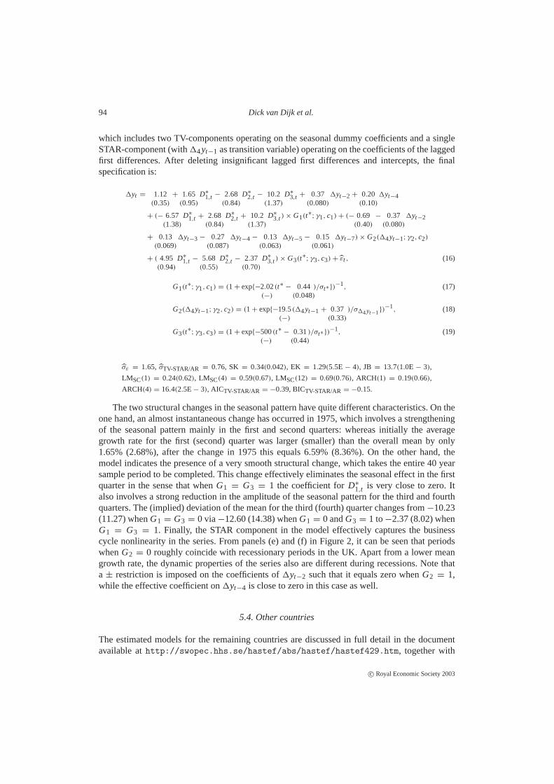
which includes two TV-components operating on the seasonal dummy coefficients and a singleSTAR-component (with14yt−1 as transition variable) operating on the coefficients of the laggedfirst differences. After deleting insignificant lagged first differences and intercepts, the finalspecification is:

1yt = 1.12(0.35)

+ 1.65(0.95)

D∗1,t − 2.68

(0.84)D∗

2,t − 10.2(1.37)

D∗3,t + 0.37

(0.080)1yt−2 + 0.20

(0.10)1yt−4

+ (− 6.57(1.38)

D∗1,t + 2.68

(0.84)D∗

2,t + 10.2(1.37)

D∗3,t ) × G1(t∗; γ1, c1) + (− 0.69

(0.40)− 0.37

(0.080)1yt−2

+ 0.13(0.069)

1yt−3 − 0.27(0.087)

1yt−4 − 0.13(0.063)

1yt−5 − 0.15(0.061)

1yt−7) × G2(14yt−1; γ2, c2)

+ ( 4.95(0.94)

D∗1,t − 5.68

(0.55)D∗

2,t − 2.37(0.70)

D∗3,t ) × G3(t∗; γ3, c3) + εt , (16)

G1(t∗; γ1, c1) = (1 + exp{−2.02(−)

(t∗ − 0.44(0.048)

)/σt∗ })−1, (17)

G2(14yt−1; γ2, c2) = (1 + exp{−19.5(−)

(14yt−1 + 0.37(0.33)

)/σ14yt−1})−1, (18)

G3(t∗; γ3, c3) = (1 + exp{−500(−)

(t∗ − 0.31(0.44)

)/σt∗ })−1, (19)

σε = 1.65, σTV-STAR/AR = 0.76, SK = 0.34(0.042), EK = 1.29(5.5E − 4), JB = 13.7(1.0E − 3),

LMSC(1) = 0.24(0.62), LMSC(4) = 0.59(0.67), LMSC(12) = 0.69(0.76), ARCH(1) = 0.19(0.66),

ARCH(4) = 16.4(2.5E− 3), AICTV-STAR/AR = −0.39, BICTV-STAR/AR = −0.15.

The two structural changes in the seasonal pattern have quite different characteristics. On theone hand, an almost instantaneous change has occurred in 1975, which involves a strengtheningof the seasonal pattern mainly in the first and second quarters: whereas initially the averagegrowth rate for the first (second) quarter was larger (smaller) than the overall mean by only1.65% (2.68%), after the change in 1975 this equals 6.59% (8.36%). On the other hand, themodel indicates the presence of a very smooth structural change, which takes the entire 40 yearsample period to be completed. This change effectively eliminates the seasonal effect in the firstquarter in the sense that whenG1 = G3 = 1 the coefficient forD∗

1,t is very close to zero. Italso involves a strong reduction in the amplitude of the seasonal pattern for the third and fourthquarters. The (implied) deviation of the mean for the third (fourth) quarter changes from−10.23(11.27) whenG1 = G3 = 0 via−12.60 (14.38) whenG1 = 0 andG3 = 1 to−2.37 (8.02) whenG1 = G3 = 1. Finally, the STAR component in the model effectively captures the businesscycle nonlinearity in the series. From panels (e) and (f) in Figure 2, it can be seen that periodswhenG2 = 0 roughly coincide with recessionary periods in the UK. Apart from a lower meangrowth rate, the dynamic properties of the series also are different during recessions. Note thata ± restriction is imposed on the coefficients of1yt−2 such that it equals zero whenG2 = 1,while the effective coefficient on1yt−4 is close to zero in this case as well.

5.4. Other countries

The estimated models for the remaining countries are discussed in full detail in the documentavailable athttp://swopec.hhs.se/hastef/abs/hastef/hastef429.htm, together with



a brief account of the most important modelling events or decisions made during the modellingcycle. To illustrate the main implications of the models for the seasonal patterns in industrialproduction in these countries, Figure 3 shows the seasonal component in the estimated TV-STARmodels for Canada, France and Italy.

The TV-STAR model for France shows a slowly changing seasonal pattern with decreasingamplitude. The deterministic component obtained from the model for Canadian output is suchthat the amplitude of the seasonal pattern first slowly increases until a rapid decrease takes placein the late 1980s. For Italy we find a similar pattern, with seasonality becoming more pronouncedduring the second half of the 1970s, followed by a swift (but relatively small) decline in theamplitude in 1994. Finally, for the US we find that allowing for nonlinearity in the autoregressivestructure eliminates all evidence suggesting that the seasonal pattern varies over time due tounspecified reasons or over the business cycle.

6. FINAL REMARKS

The results of this paper suggest that seasonal patterns in quarterly industrial production seriesfor the G7 countries have been changing over time. On the other hand, business cycle fluctuationsdo not seem to be the main cause for this change. Our findings are in contrast with Canova andGhysels (1994) and Franses (1996), who considered US output and concluded that the businesscycle influences the seasonal cycle. Similarly, Cecchettiet al. (1997) found that in the USseasonal fluctuations in production and inventories vary with the state of the business cycle. Thereare at least two reasons for differences between our results and those of the above authors. First,they only considered US series and included the GNP and inventories. The second, and perhapsthe most important, reason is that those authors did not consider causes other than business cyclefluctuations. Less restrictive considerations appear to lead to rather different conclusions.

It seems possible to reconcile our results with the findings of Matas-Mir and Osborn (2001).An important detail is that they used monthly series, whereas ours are quarterly. As the authorsexplain, a business-cycle induced change in summer months, visible in monthly series, can besubstantially masked at a quarterly frequency. Another reason for the differences in results isthat Matas-Mir and Osborn (2001) implicitly give a preference to business-cycle induced patternshifts, because other types of change are only described by linear trends in seasonal dummycoefficients. This may be too rigid a solution and a more flexible parameterization, offered bythe TV-STAR model, is needed to fully assess the role and significance of institutional andtechnological change in seasonal patterns of the series considered here. Thus the differencesin results between Matas-Mir and Osborn (2001) and our work may to a large extent be ascribedto differences in the emphasis, reflected both in the frequency of the series and the choice ofmodel.

As the ‘Kuznets-type’ unspecified change in seasonal patterns is in our work proxied bytime, we cannot give a definite answer to the question of what kind of change, technological,institutional, or ‘other’, has been important in the industrial output series we have investigated.The importance of our results lies in the fact that they make us aware of changes such as thegradual decrease in amplitude many series are showing. Some speculation about the reasonsfor this may be allowed. There is evidence of changes in inventory management affectingthe seasonal pattern of industrial output. Carpenter and Levy (1998) showed that inventoryinvestment and output are highly correlated not only at business cycle frequencies but also atseasonal frequencies. Given the importance of inventories for (changes in) fluctuations in output



Figure 3. Characteristics of TV-STAR model for quarterly industrial production growth rates in Canada,France and Italy.



(see Sichel (1994) and McConnell and Perez Quiros (2000), among others), it may well be thatchanges in inventory management such as the use of ‘just-in-time’ techniques have dampenedthe seasonal cycle in inventory investment and thereby affected the seasonal cycle in production.

On the other hand, very abrupt changes, such as the one in the German industrial outputseries in 1978, may most naturally be ascribed to the agency producing the data, unless otherinformation about the nature of the change is available. In general, it may sometimes be relativelyeasy to suggest individual causes for shifts in the seasonal pattern at the industry level. Becauseof aggregation this becomes more difficult where the volume of the total industrial output isconcerned.

The results also give rise to the question of how the current seasonal adjustment methodscope with series with time-varying seasonality. One may also ask what the consequences of suchvariation are on using seasonally adjusted series in macroeconomic modelling. Investigating thisquestion in the present context, however, must be left for future work. On the other hand, themodels estimated for seasonally unadjusted first differences in this work cannot be expected tobe useful in forecasting the volume of industrial production. Models that enhance and explainthe low-frequency fluctuations in the series are better suited for that purpose.

ACKNOWLEDGEMENTS

Financial support from the Jan Wallander’s and Tom Hedelius’ Foundation for Social Research,Contract No. J99/37, is gratefully acknowledged. The first author acknowledges financialsupport from the Netherlands Organization for Scientific Research (N. W. O.). The third authoracknowledges financial support from the Swedish Council for Research in the Humanities andSocial Sciences. We thank Jan Tore Klovland for bringing Gjermoe (1926) to our attention.We have also benefited from helpful comments and suggestions by the editor, an anonymousreferee, Eilev Jansen and participants at the conferences ‘Growth and Business Cycles in Theoryand Practice’, Manchester, June 2000, ‘Seasonality in Economic and Financial Variables’,Faro, October 2000, the ‘Third Workshop on New Approaches to the Study of EconomicFluctuations’, Hydra, May 2001, the Annual Conference of the European Economic Association,Lausanne, August 2001, and a seminar at Bilkent University, Ankara. Any remaining errors andshortcomings in the paper are ours.

REFERENCES

Canova, F. and E. Ghysels (1994). Changes in seasonal patterns: are they cyclical?Journal of EconomicDynamics and Control 18, 1143–71.

Canova, F. and B. E. Hansen (1995). Are seasonal patterns constant over time? A test for seasonal stability.Journal of Business & Economic Statistics 13, 237–52.

Carpenter, R. E. and D. Levy (1998). Seasonal cycles, business cycles, and the comovement of inventoryinvestment and output.Journal of Money, Credit and Banking 30, 331–46.

Cecchetti, S. G. and A. K. Kashyap (1996). International cycles.European Economic Review 40, 331–60.Cecchetti, S. G., A. K. Kashyap and D. W. Wilcox (1997). Interactions between the seasonal and business

cycles in production and inventories.American Economic Review 87, 884–92.Franses, P. H. (1996).Periodicity and Stochastic Trends in Economic Time Series. Oxford: Oxford

University Press.



Gjermoe, E. (1926). Arbeidsledigheten og arbeidsledighetsstatistikken in Norge.Statistiske meddelser 44,82–100.

Gjermoe, E. (1931). Det konjunkturcykliske element: beskjeftigelsegradens sesongbevegelse.Statsøkonomisk tidskrift 49, 45–82.

Granger, C. W. J. and T. Terasvirta (1993).Modelling Nonlinear Economic Relationships. Oxford: OxfordUniversity Press.

Hansen, B. E. (1996). Inference when a nuisance parameter is not present under the null hypothesis.Econometrica 64, 413–30.

Harvey, A. C. (1989).Forecasting, Structural Time Series Models and the Kalman Filter. Cambridge:Cambridge University Press.

Harvey, A. C. and A. Scott (1994). Seasonality in dynamic regression models.Economic Journal 104,1324–45. Cambridge: Cambridge University Press.

Hylleberg, S. (1994). Modelling seasonal variation. In C. P. Hargreaves (ed.),Nonstationary Time SeriesAnalysis and Cointegration. Oxford: Oxford University Press.

Krane, S. and W. Wascher (1999). The cyclical sensitivity of seasonality in US employment.Journal ofMonetary Economics 44, 523–53.

Kuznets, S. (1932). Seasonal pattern and seasonal amplitude: measurement of their short-term variation.Journal of the American Statistical Association 27, 9–20.

Lundbergh, S., T. Terasvirta and D. van Dijk (2003). Time-varying smooth transition autoregressive models.Journal of Business & Economic Statistics 21, 104–21.

Luukkonen, R., P. Saikkonen and T. Terasvirta (1988). Testing linearity against smooth transition autore-gressive models.Biometrika 75, 491–9.

Matas-Mir, A. and D. R. Osborn (2001). Does seasonality change over the business cycle? An investigationusing monthly industrial production series. University of Manchester, Centre for Growth and BusinessCycle Research Discussion Paper Series, No. 9.

McConnell, M. M. and G. Perez Quiros (2000). Output fluctuations in the United States: what has changedsince the early 1980s?American Economic Review 90, 1464–76.

Miron, J. A. (1996).The Economics of Seasonal Cycles. Cambridge, MA: MIT Press.Miron, J. A. and J. J. Beaulieu (1996). What have macroeconomists learned about business cycles from the

study of seasonal cycles?Review of Economics and Statistics 78, 54–66.Pierce, D. A. (1978). Seasonal adjustment when both deterministic and stochastic seasonality are present.

In A. Zellner (ed.),Seasonal Analysis of Economic Time Series. pp. 242–69. Washington, DC: USDepartment of Commerce, Bureau of the Census.

Sichel, D. E. (1994). Inventories and the three phases of the business cycle.Journal of Business andEconomic Statistics 12, 269–77.

Terasvirta, T. (1998). Modelling economic relationships with smooth transition regressions. In A. Ullah andD. E. A. Giles (eds),Handbook of Applied Economic Statistics. pp. 507–552. New York: Marcel Dekker.

van Dijk, D., T. Terasvirta and P. H. Franses (2002). Smooth transition autoregressive models—a surveyof recent developments.Econometric Reviews 21, 1–47.


Documents

The effects of institutional and technological change and business cycle fluctuations on seasonal patterns in quarterly industrial production series