THE EFFECTS OF MICRO- AND MACRO-SCALE GEOMETRIC PARAMETERS …

Virginia Commonwealth University Virginia Commonwealth University

VCU Scholars Compass VCU Scholars Compass

Theses and Dissertations Graduate School

2012

THE EFFECTS OF MICRO- AND MACRO-SCALE GEOMETRIC THE EFFECTS OF MICRO- AND MACRO-SCALE GEOMETRIC

PARAMETERS ON PERFORMANCE OF THE PLEATED AEROSOL PARAMETERS ON PERFORMANCE OF THE PLEATED AEROSOL

FILTERS FILTERS

Shahryar Fotovati Virginia Commonwealth University

Follow this and additional works at: https://scholarscompass.vcu.edu/etd

Part of the Engineering Commons

© The Author

Downloaded from Downloaded from https://scholarscompass.vcu.edu/etd/2681

This Dissertation is brought to you for free and open access by the Graduate School at VCU Scholars Compass. It has been accepted for inclusion in Theses and Dissertations by an authorized administrator of VCU Scholars Compass. For more information, please contact [email protected].

http://www.vcu.edu/

http://www.vcu.edu/

https://scholarscompass.vcu.edu/

https://scholarscompass.vcu.edu/etd

https://scholarscompass.vcu.edu/gradschool

https://scholarscompass.vcu.edu/etd?utm_source=scholarscompass.vcu.edu%2Fetd%2F2681&utm_medium=PDF&utm_campaign=PDFCoverPages

http://network.bepress.com/hgg/discipline/217?utm_source=scholarscompass.vcu.edu%2Fetd%2F2681&utm_medium=PDF&utm_campaign=PDFCoverPages

https://scholarscompass.vcu.edu/etd/2681?utm_source=scholarscompass.vcu.edu%2Fetd%2F2681&utm_medium=PDF&utm_campaign=PDFCoverPages

mailto:[email protected]

School of Engineering

Virginia Commonwealth University

This is to certify that the Dissertation prepared by Shahryar Fotovati entitled THE

EFFECTS OF MICRO- AND MACRO-SCALE GEOMETRIC PARAMETERS ON

PERFORMANCE OF THE PLEATED AEROSOL FILTERS has been approved by his

or her committee as satisfactory completion of the thesis or dissertation requirement for

the degree of Doctor of Philosophy

Dr. Hooman V. Tafreshi, School of Engineering

_______________________________________________________________________ Dr. Gary C. Tepper, School of Engineering

Dr. Ramana M. Pidaparti, School of Engineering

Dr. P. Worth Longest, School of Engineering

Dr. Stephen S. Fong, School of Engineering

Dr. Umit Ozgur, School of Engineering

Dr. J. Charles Jennett, Dean of the School of Engineering

Dr. F. Douglas Boudinot, Dean of the School of Graduate Studies

MARCH 12, 2012

© Shahryar Fotovati, 2012

All Rights Reserved

THE EFFECTS OF MICRO- AND MACRO-SCALE GEOMETRIC PARAMETERS

ON PERFORMANCE OF THE PLEATED AEROSOL FILTERS

A Dissertation submitted in partial fulfillment of the requirements for the degree of

Doctor of Philosophy at Virginia Commonwealth University.

by

SHAHRYAR FOTOVATI

MS in Mechanical Engineering, Shiraz University, IR, 2007

BS in Mechanical Engineering, Persian Gulf University, IR, 2001

Director: HOOMAN V. TAFRESHI

QIMONDA ASSISTANT PROFESSOR, DEPARTMENT OF MECHANICAL AND

NUCLEAR ENGINEERING

Virginia Commonwealth University

Richmond, Virginia

March 2012

ii

Acknowledgement

First and foremost, I offer my sincere gratitude to my supervisor, Dr. Hooman V.

Tafreshi, who has supported me throughout my PhD studies with his patience and

knowledge while allowing me the room to work in my own way. I attribute the level of

my PhD degree to his encouragement, enthusiasm, and immense knowledge. One simply

could not wish for a better or friendlier supervisor.

Besides my advisor, I would like to thank the rest of my thesis committee: Professor

Tepper, Professor Longest, Professor Pidaparti, Professor Fong, and Professor Ozgur, for

their insightful comments, and hard questions.

This work was supported by The Nonwovens Institute at NC State University. Their

financial supports are highly appreciated.

Last but not least, I would like to thank my family: my parents, Mahvash and Shahram,

my sister, Shahrzad and my beautiful Morvarid for supporting me spiritually throughout

my life. They always soften the life difficulties for me. I owe all my achievements to

them and I am happy to devote this work to them.

iii

Table of Contents

Page

List of Tables ..................................................................................................................... vi

List of Figures ................................................................................................................... vii

Chapter

1 Background and introductions ...........................................................................3

1.1 Aerosol filtration from a micro-scale point of view ................................3

1.2 Aerosol filtration from a macro-scale point of view .............................11

2 Micro-scale modeling of poly-dispersed fibrous media ..................................20

2.1 Introduction ...........................................................................................20

2.2 Unimodal equivalent diameters of bimodal media ................................21

2.3 Governing equations ..............................................................................24

2.4 Numerical approach ..............................................................................26

2.5 Results and discussions .........................................................................30

2.6 Experimental validation ........................................................................35

2.7 Conclusions ...........................................................................................36

3 Micro-scale modeling of filter media with different fiber orientations ...........51

3.1 Introduction ...........................................................................................51

3.2 Numerical simulations ...........................................................................53

3.3 Analytical expressions for filter performance .......................................57

iv


3.5 Conclusions ...........................................................................................64

4 Micro-scale modeling of media made of multi-lobal fibers ............................72

4.1 Introduction ...........................................................................................72

4.2 Equivalent circular fiber diameter for trilobal fibers .............................73

4.3 CFD simulations ....................................................................................76


4.5 Conclusions ...........................................................................................86

5 Macro-scale modeling of surface-dust loading in pleated filters .....................99

5.1 Introduction ...........................................................................................99

5.2 Pleated geometry and flow field ..........................................................100

5.3 Modeling dust deposition ....................................................................102

5.4 Results and discussions .......................................................................104

5.5 Conclusions .........................................................................................116

6 Macro-scale modeling of pleated depth filters ...............................................136

6.1 Introduction .........................................................................................136

6.2 Flow field and particle tracking ...........................................................138

6.3 Macro-scale modeling of dust loaded fibrous media ..........................141

6.4 Model implementation and validation .................................................145

v


6.6 Conclusions .........................................................................................151

7 Macro-scale modeling of pleated filters challenged with poly-disperse

aerosols ......................................................................................................163

7.1 Introduction .........................................................................................163

7.2 Modeling dust deposition ....................................................................165

7.3 Poly-dispersed particle consideration ..................................................167


7.5 Conclusions .........................................................................................173

8 Overall Conclusions .......................................................................................181

Literature Cited ................................................................................................................185

Appendices .......................................................................................................................191

A Granular filtration ..........................................................................................191

vi

List of Tables

Page

Table 1.1a: Commonly used expressions for dimensionless pressure drop.......................16

Table 1.1b: Commonly used expressions for permeability. ..............................................16

Table 1.2: Expressions for SFE due to Brownian diffusion. .............................................17

Table 1.3: Expressions for SFE due to interception. .........................................................17

Table 1.4: Expressions for SFE due to inertial impaction. ................................................18

Table 2.1: Sum of the squares of differences between experiment and formulation for

ln( )/P t ................................................................................................................................38

Table 2.2: Pressure drop results for blends of A-fibers and D-fibers ................................38

Table 2.3: Pressure drop results for blends of B-fibers and D-fibers ................................38

Table 3.1: Pressure drop per thickness (kPa/m) of media with different in-plane fiber

orientations. Fiber diameter, and SVF, and face velocity are 10 µm, 7.5%, and 0.1 m/s,

respectively. .......................................................................................................................66

Table 3.2: Pressure drop per thickness (kPa/m) of media with different through-plane

fiber orientations. Fiber diameter, and SVF, and face velocity are 10 µm, 7.5%, and 0.1

m/s, respectively. ...............................................................................................................66

Table 4.1: Pressure drop of the media shown in Figure 4.15. Prediction of the empirical

correlation of Davies (1973), obtained for media with circular fibers, is also added. .......87

Table 5.1: Different fibrous media considered for this study. .........................................118

vii

List of Figures

Page

Figure 1.1: Graphical demonstration for single fiber efficiency ........................................18

Figure 1.2: Pleated geometry (a) Rectangular geometry, (b) Triangular geometry ...........19

Figure 1.3: Dual scale configuration of a pleated medium ................................................19

Figure 2.1: An equivalent unimodal fibrous structure (right figure) for each bimodal (poly

dispersed) filter medium (left figure) .................................................................................39

Figure 2.2: a) Square unit cell with one fine and three coarse fibers (cn = 0.75); b)

simulation domain and boundary conditions; c) three possible fiber arrangements of

columns, rows and staggered configurations for the case of cn = 0.5 ...............................39

Figure 2.3: a) Contour plot of particle concentration (%) with 10pd nm; b) trajectories

for 2 µm particles; c) particle trajectories in the first unit cell. The filter is made up of

fibers of 1 and 3 micron diameter with an SVF of 10% ....................................................40

Figure 2.4: Effect of inlet particle number density (mesh density) on particle penetration

calculated via Lagrangian Method .....................................................................................41

Figure 2.5: A comparison between the efficiency of unimodal medium and analytical

expressions .........................................................................................................................41

Figure 2.6: Pressure drop per unit thickness of bimodal media .........................................42

Figure 2.7: Penetration per unit thickness of different bimodal filters with different fiber

diameter ratios and coarse fiber number (mass) fractions for Brownian particles ............43

viii


diameter ratios and coarse fiber number (mass) fractions of 0 5cn . ...............................44

Figure 2.9: Figure of merit of different bimodal filters with different cfR and cn ..............45

Figure 2.10: An example of our Poly-disperse fibrous medium with fiber diameters in the

range of 2–10µm. Streamlines are shown to illustrate the flow ........................................46

Figure 2.11: Diffusion (left) and interception (right) efficiency of mono-modal filters

with 2fd µm in comparison with existing semi-empirical expressions ........................47

Figure 2.12: Diffusion (left) and interception (right) efficiency of mono-modal filters

with 10fd µm in comparison with existing semi-empirical expressions .......................47

Figure 2.13: Particle collection efficiency for three different SVFs ..................................48

Figure 2.14: Results of fiber diameter measurements .......................................................49

Figure 2.15: Comparison between experimental collection efficiency and predicted values

using unimodal expressions with different equivalent definitions (Blends of A & D

fibers) .................................................................................................................................50

Figure 3.1: Fibrous structures (a) Parallel (b) Layered (c) 3-D random arrangement .......67

Figure 3.2: Three-D fibrous structures with (a) o15 (b) o30 (c) o45 in-plane and (d) o15 (e)

o30 (f) o45 through-plane fiber orientations ......................................................................67

Figure 3.3: An example of the computational domains considered in this work along with

the boundary conditions. ....................................................................................................68

ix

Figure 3.4: Effects of fibers’ in-plane orientation on the collection efficiency of media

with zero Through-plane orientation for (a) nano particles, (b) micron-size particles ......68

Figure 3.5: An example of unidirectional fibrous strictures (flow perpendicular to the

fibers axis) ..........................................................................................................................69

Figure 3.6: Effects of fibers’ through-plane orientation on the particle collection

efficiency of media with zero in-plane fiber orientation ...................................................69

Figure 3.7: Figure of Merit (FOM) of media with different in-plane (a-b) and through-

plane (c) fiber orientations. Fiber diameter, and SVF, and face velocity are 10 µm, 7.5%,

and 0.1 m/s, respectively ....................................................................................................70

Figure 3.8: Figure of Merit (FOM) of media with different in-plane fiber orientations, at

two different face velocities of 0.01 and 1 m/s, respectively.............................................71

Figure 3.9: Figure of Merit (FOM) of media with different through-plane fiber

orientations, at two different face velocities of 0.01 and 1 m/s, respectively. Fiber

diameter and SVF are 10 µm and 7.5%, respectively ........................................................71

Figure 4.1: a) trilobal fiber, source: http://www.fiberwebfiltration.com/Reemay.cfm, b)

overlapping ellipses forming a trilobal cross-section ........................................................87

Figure 4.2: Equivalent circular diameters obtained based on equal surface area and equal

perimeter are compared with the diameter of the circumscribed circle for trilobal fibers

with different aspect ratios and two different minor axes of b=2 and 4 micrometer. It can

x

be seen that equivalent diameter based on equal perimeter is very close to the diameter of

the circumscribed circle .....................................................................................................88

Figure 4.3: Our program’s flowchart for generating media with random trilobal fibers ...89

Figure 4.4: An example of our simulation domains consisting of 300 trilobal fibers with

an aspect ratio of 1.5 randomly placed in square domain resulting in an SVF of 10% .....89

Figure 4.5: (a) Contours of nano-particle concentration are shown in a trilobal medium

with an SVF of 10% consisting of fibers with an aspect ratio of 2. (b) Few particle

trajectories are shown to demonstrate particle collection due to interception ...................90

Figure 4.6: Influence of grid density on the pressure drop cause by a single fiber placed in

a domain with an SVF of 10% as shown in the inset .........................................................91

Figure 4.7: Influence of number of particles injected at the inlet on the penetration

prediction of a typical trilobal media simulated in this study (SVF of 10% and aspect

ratio of 2)............................................................................................................................91

Figure 4.8: Comparison between simulation results obtained for trilobal filters with SVF

of 10% and aspect ratio of 2 and their equivalent circumscribed media. Predictions of the

semi-empirical expressions of Stechkina and Fuchs (1965) and Lee and Liu (1982) are

added for comparison .........................................................................................................92

Figure 4.9: Deflection of the streamlines is mostly caused by the projected area of the

fibers on a plane normal to the flow direction. It can be seen that the flow pattern around

(a) a trilobal fiber and, (b) its circumscribed circle, are quite similar ...............................92

xi

Figure 4.10: Penetration per thickness for trilobal media and their equivalent area-based

and circumscribed media at a constant SVF of 10% (figures a–c), and at a constant aspect

ratio of 2 (figures d–f) ........................................................................................................93

Figure 4.11: Relationship between pressure drop of trilobal media and their equivalent

circumscribed equivalents for a SVF of 10% and different aspect ratios of 1.5, 2, 2.5 and

3. Curve fitting equations are given for each case for convenience ..................................94

Figure 4.12: Relationship between SVF of trilobal filters with different aspect ratios and

different minor axis diameter, and those of their circumscribed equivalent media ...........94

Figure 4.13: Pressure drop per thickness for trilobal filters and their circumscribed

equivalent media before and after pressure correction. .....................................................95

Figure 4.14: Trilobal fibers with different 1r values created with the mathematical

formulation which is used by Geodict software ................................................................95

Figure 4.15: 3-D fibrous media with trilobal fibers having an aspect ratio of 1.5 and an

SVF of 10% (a) and, circumscribed (b) and area-based equivalent media (c) ..................96

Figure 4.16: (a) Penetration per thickness and, (b) FOM calculated for the media shown

in the previous figure .........................................................................................................97

Figure 4.17: Star-shape fibers ............................................................................................97

Figure 4.18: Penetration of star-shaped fibers and their equivalent circumscribed. ..........98

Figure 4.19: Relationship between pressure drop of star-shaped media and their

equivalent circumscribed. ..................................................................................................98

xii

Figure 5.1: Simulation domain for a) rectangular pleats, and b) triangular pleats ..........118

Figure 5.2: Pressure drop of clean filters with U-shaped and V-shaped pleats with

different pleat counts at two different air inlet velocities of 0.2 and 1 m/s. The filter media

considered here have layered micro-structures (see Table 5.1) .......................................119

Figure 5.3: Pressure drop of clean filters with U-shaped and V-shaped pleats with

different pleat counts at two different air inlet velocities of 0.2 and 1 m/s. The filter media

considered here have three-dimensionally isotropic micro-structures (see Table 5.1) ....120

Figure 5.4: Dust cake deposition pattern and air streamlines inside rectangular and

triangular pleats with a) 4 pleats/ inch, b) 20 pleats/ inch, c) 15o pleat angle, and d) 4

o

pleat angle. Particle diameter and flow velocity are 3µm and 0.2 m/s, respectively .......121



o

pleat angle. Particle diameter and flow velocity are 10µm and 0.2 m/s, respectively .....122



o

pleat angle. Particle diameter and flow velocity are 10µm and 1 m/s, respectively ........123

Figure 5.7: Streamwise velocity magnitude on the centerline of pleat channels for a)

rectangular pleats, b) triangular pleats. The inlet velocity is 0.2 m/s ..............................124

Figure 5.8: Dust cake distribution along the x-direction inside rectangular and triangular

pleat geometries ...............................................................................................................125

xiii

Figure 5.9: Pressure drop increase during particle loading with rectangular and triangular

pleats for particles with pd of 3 and 10µm and inlet velocities of 0.2 and 1 m/s ............126

Figure 5.10: Pressure drop increase during particle loading with rectangular and

triangular pleats. The dust cake is assumed to be three times more permeable than the

fibrous media ...................................................................................................................127

Figure 5.11: Dust cake deposition pattern and air streamlines inside filters with 15

rectangular or triangular pleats per inch loaded with particles having 3 and 10µm

diameters with air velocities of 0.2 and 1 m/s .................................................................128

Figure 5.12: Comparison between the pressure drop increase for filters with 15

rectangular and triangular pleats per inch loaded with particles having 3 and 10µm

diameters with air velocities of 0.2 and 1 m/s .................................................................129

Figure 5.13: Clean filter pressure drop for pleat angles of 15o, 10

o, 8

o, 5

o, 4

o and 3

o,

regarding to different pleat heights ..................................................................................130

Figure 5.14: Clean filter centerline velocity profile for pleat angles of 15o, 10

o, 8

o, 5

o, 4

o

and 3o for different pleat heights ......................................................................................131

Figure 5.15: Clean filter face velocity profile for pleat angles 15o, 10

o, 8

o, 5

o, 4

o and 3

o

regarding to different pleat heights ..................................................................................132

Figure 5.16: Graphical dust pattern and streamlines for pleat angle of 15o and inlet

velocity of 0.2 m/s with 10µm injected particles .............................................................133

xiv

Figure 5.17: Graphical dust pattern and streamlines for pleat angle of 3o and inlet velocity

of 0.2 m/s with 10µm injected particles ...........................................................................134

Figure 5.18: Pressure drop increase ratio respect to number of time steps for injected

particles with 10µm diameter and 0.2m/s inlet velocity for pleat angles of 15o, 10

o, 8

o, 5

o,

4o and 3

o ...........................................................................................................................135

Figure 6.1: Simulation domain for triangular pleats with a pleat angle of 2θ and a pleat

height of L ......................................................................................................................153

Figure 6.2: Schematic illustration of transient particle deposit increase inside each

computational cell ............................................................................................................153

Figure 6.3: Numerical simulation flow chart. At each stage, the effective UDF has been

mentioned. ........................................................................................................................154

Figure 6.4: Comparison between our simulation outputs and the cell model semi-

empirical equations for particle penetration through a clean fibrous medium. The cell

model equations are shown in Chapter 1 .........................................................................155

Figure 6.5: Contour plots of cell SVF together with air streamlines showing an example

of particle deposition inside the fibrous zone at two different simulation times of 40t s

(a), and 180t s (b). The simulations are conducted with a particle diameter of

10pd µm at a speed of 0 05inu . m/s. The fibrous medium is assumed to have a SVF

xv

of 5% and a fiber diameter of 15fd µm with the thickness of 0.7mm. Maximum

allowable SVF is obtained accordingly from Equation 6.10 ...........................................156

Figure 6.6: Comparison between our pressure drop predictions and those of the semi-

empirical expression of Thomas et al. (2001) for fibrous flat sheets during dust

deposition. The fibrous medium is assumed to have a SVF of 5%, a fiber diameter of

15fd µm, and a thickness of 0.7mm ............................................................................157

Figure 6.7: Our collection efficiency predictions are used along with the semi-empirical

expression of Kanaoka et al. (1980) for particle penetration through fibrous flat sheets

during dust deposition. The curve fitting parameters are (a) λ=5000, (b) λ=3000, (c)

λ=250, and (d) λ=500. The fibrous medium is assumed to have a SVF of 5%, a fiber

diameter of 15fd µm, and a thickness of 0.7mm .........................................................158

Figure 6.8: Particle penetration per thickness obtained for clean filters with different pleat

counts at two different air inlet velocities of 0.05 and 0.5 m/s ........................................159

Figure 6.9: Effects of pleat count of the face velocity (a) and pressure drop (b) obtained

for clean filters at two different air inlet velocities of 0.05 and 0.5 m/s. Fibrous media

have a SVF of 5%, a fiber diameter of 15fd µm, a thickness of 0.7 mm .....................159


of particle deposition inside the fibrous zone in a pleated filter. The particle diameter and

xvi

air inlet velocity are considered to be 3pd µm and 0 05inu . m/s, respectively. Here

SVF is 5%, fiber diameter is 15fd µm, and thickness of 0.7 mm ..............................160

Figure 6.11: Instantaneous pressure drop versus time for two different particle diameters

of 100 nm and 3µm, and at two different air inlet velocities of 0.05 and 0.5m/s ............161

Figure 6.12: Instantaneous penetration versus time for two different particle diameters of

100 nm and 3µm, and at two different air inlet velocities of 0.05 and 0.5m/s ................162

Figure 7.1: Flow chart which describes poly-dispersed particle deposition ....................175

Figure 7.2: Graphical demonstration for mono-dispersed dust deposition pattern inside

filters 4, 8 and 12 pleats/in with (a) 1µm particles and 0.05 m/s inlet velocity and, (b)

10µm particles and 0.5 m/s inlet velocities ......................................................................176

Figure 7.3: Performance of filters with 4, 8, and 12 pleats/in with 1µm particles (a)

Pressure drop increase ratio for 0.05 m/s inlet velocity. (b) Collection efficiency increase

ratio for 0.05 m/s inlet velocity. (c) Pressure drop increase ratio for 0.5 m/s inlet velocity.

(d) Collection efficiency increase ratio for 0.5 m/s inlet velocity ...................................177

Figure 7.4: Performance of filters with 4, 8, and 12 pleats/in with 10µm particles and 0.5

m.s-1 inlet velocities. (a) Pressure drop increase ratio. (b) Collection efficiency increase

ratio ..................................................................................................................................178

xvii

Figure 7.5: Graphical demonstration for poly-dispersed dust deposition pattern inside

filters 4, 8 and 12 pleats/in with 1–10µm particles distribution for (a) 0.05 m/s inlet

velocity and, (b) 0.5 m/s inlet velocity ............................................................................179

Figure 7.6: Performance of filters with 4, 8, and 12 pleats/in with poly-dispersed particles

(a) Pressure drop increase ratio for 0.05 m/s inlet velocity. (b) Collection efficiency

increase ratio for 0.05 m/s inlet velocity. (c) Pressure drop increase ratio for 0.5 m/s inlet

velocity. (d) Collection efficiency increase ratio for 0.5 m/s inlet velocity ....................180

1

Abstract

THE EFFECTS OF MICRO- AND MACRO-SCALE GEOMETRIC PARAMETERS ON

PERFORMANCE OF THE PLEATED AEROSOL FILTERS

By Shahryar Fotovati, M.Sc.

A Dissertation submitted in partial fulfillment of the requirements for the degree of Doctor

of Philosophy at Virginia Commonwealth University.

Virginia Commonwealth University, 2012

Major Director: Dr. Hooman V. Tafreshi

Qimonda Assistant Professor, Department of Mechanical and Nuclear Engineering

While most filters are made of pleated fibrous media, almost all existing theories of aerosol

filtration are developed for flat media placed perpendicular to the air flow. Expressions

developed for flat sheet media do not provide accurate information directly useful for

designing a pleated filter, and therefore, most progress made in developing pleated filters is

based on empiricism. This study is aimed at establishing an enabling knowledge that

allows for a better design and optimization of pleated aerosol filters. This study is focused

on developing a predictive simulation method that accounts for the influence of a filter’s

micro-scale geometric parameters, such as fiber orientation, as well as its macro-scale

2

features, like pleat shape, in predicting the transient pressure drop and collection efficiency

with or without the effects of dust loading. The dual-scale simulation method developed in

this work is believed to be the only feasible approach for design and optimization of

pleated aerosol filters with the current academic-level computational power.

Our study is divided into two major tasks of micro- and macro-scale modeling. Our micro-

scale studies are comprised of a series of CFD simulations conducted in virtual 2-D or 3-D

fibrous geometries that resemble the internal micro-structure of a fibrous medium. These

simulations are intended to isolate the effects of each micro structural parameter and study

its influence on the performance of the filter medium. In detail, it is intended to propose a

method to predict the performance of micro-structures with fiber size distribution. Also,

the effects of micro-structural fiber orientation were investigated. Moreover, we offered

methodology to predict the performance of noncircular fibers using available analytical

expressions for circular fibers. It is shown that the circumscribed circle for a trilobal

shaped fiber gives the best prediction for collection efficiency. In macro-scale simulations,

on the other hand, the filter medium is treated as a lumped porous material with its

properties obtained via micro-scale simulations. Our results showed that more number of

pleats helps better performance of pleated filters, however, if the pleat channel becomes

blocked by dust cake then this effect is no longer valid.

3

CHAPTER 1 Background Information

Many works have been devoted to study of flow in nonwoven media and model and even

optimize them especially if they are used as aerosol filters. In some studies, only the clean

structures were assumed, however, in very few, dust depositions inside media were

considered. At first, we briefly review the theory of aerosol filtration and introduce

analytical expressions which will be used for validations purposes or introduce micro-scale

parameters in macro-scale modeling in other chapters. Another part of this chapter is

focused on introducing pleated filters as they are used as our macro-scale domain.

1.1 Aerosol Filtration from a Micro-Scale Point of View

Usually, Performance of any fibrous structure is pointed by their filtration characteristics

or more specifically, their pressure drop and particles collection efficiencies. Performance

of fibrous media has been studied for many years and there are many analytical, numerical,

and/or empirical correlations available for such calculations. In almost all of these studies a

fibrous medium is assumed to be made up of fibers with a unimodal circular fiber diameter

distribution (referred to as unimodal or mono dispersed medium here), placed normal to

the flow. It is more general to refer to permeability (inversely proportional to pressure

drop) of a medium instead of pressure drop. There are various well-known models for

predicting the pressure drop or permeability of such media. In almost all permeability

models, permeability of unimodal media, k , is presented as a function of fiber radius, r ,

4

and Solid Volume Fraction (SVF),α , of the media regardless of dust deposition(Tafreshi et

al. 2009, Jaganathan et al. 2008):

2

1

( )

k

r f α (1.1)

Where, ( )f α is referred to as dimensionless pressure drop and is only a function of solid

volume fraction.

Collection efficiency of a fibrous structure is defined as the fraction of the particles which

were captured by the fibrous medium. Knowing the number (concentration) of the particles

at the inlet and outlet gives us the collection efficiency of fibrous medium:

inlet outlet

inlet

N NE

N (1.2)

It is common to relate the collection efficiency to the penetration, the penetration is:

outlet

inlet

NP

N (1.3)

and therefore the collection efficiency is:

1E P (1.4)

1.1.1 Pressure Drop of the Clean Fibrous Structures

One of the most popular methods to predict the pressure drop of fibrous media is based on

the single fiber theory. In this method, according to pressure drop of a single circular fiber,

the total filter pressure drop will be estimated. In pioneering works done by Kuwabara

5

(1959) and Happel (1959), cell model was proposed to obtain an acceptable prediction for

performance of a single fiber. In this model, parallel circular cylinders are distributed

randomly and homogeneously in a viscous flow. They considered a circular cylindrical

fiber enclosed by imaginary coaxial circle. In that model, the Stokes approximation was

used to define the stream function as:

3B rψ Ar C ln Dr sinθ

r R (1.5)

where A , B , C and D are constants to be found. The stream functionψ , was obtained by the

general solution for Stokes flow equation which is as:

22

2 2

1 10r ψ

r r r r θ (1.6)

Kuwabara assumed the vorticity to vanish at the outer boundary, and found the constants in

equation (1.5) and he proposed the dimensionless pressure drop to be as:

4αf α

Ku (1.7)

Ku in equation (1.7) is Kuwabara factor which can be expressed as:

21ln 0.75

2 4Ku (1.8)

Happel used a given tangential stress and found constants in equation (1.5) and came up

with the following expression for dimensionless pressure drop:

2

2

4

1 1 1

2 2 1

αf α

αln α

α

(1.9)

6

Works of Kuwabara and Happel are limited to some special boundary conditions that they

assumed. Other definitions for dimensionless pressure drop proposed and are available in

literature inspired by work of Kuwabara, but for more general arrangements of fibers.

Henry and Ariman (1983) numerically solved the flow field around a staggered array of

parallel circular cylindrical fibers and offered the following for dimensionless pressure

drop:

2 32 446 38 16 138 9f α . α . α . α (1.10)

One of the most important correlations for dimensionless pressure drop for randomly

oriented layered fibrous structure was proposed by Davis (1973) which holds for vast

range of solid volume fractions of 0.6% to 30%:

3 2 364 1 56/f α α α (1.11)

Some other important expressions for dimensionless pressure drop have been listed in

Table 1.1a, as well. In that table, ff d/λKn 2 is the fiber Knudsen number, where λ is the

molecular mean free path of air (about 64 nm in normal temperatures and pressures)

and fd is fiber diameter.

In Table 1.1b, the presented common equations give permeability explicitly. In those

equations, 0K and 1K are zeroth and first order Bessel functions of the second kind, whereas

layTPk and lay

IPk are permeability constants in the through-plane and in-plane directions,

respectively. By through-plane, this means that the permeability is in the normal direction

to the fibrous plane, where, in-plane refers to the direction parallel with the fibrous plane.

7

The superscript “iso” is used to denote the permeability of a randomly 3-D fibrous

medium. In these equations, is the solid volume fraction of the media and r is the fiber

radius. Other expressions can be found in literature which we avoid to mention them here

for brevity (Jackson and James 1986, Rao and Faghri 1988). Using the dimensionless

pressure drop, the total filter pressure drop according to Darcy’s law (Dullien, 1992) will

be achieved as follow:

2Δ

μUtp f a

r (1.12)

In above expression, μ is viscosity related to the flow, U is the flow face velocity (velocity

normal to the fibrous domain) and t is the fibrous domain thickness.

1.1.2 Collection Efficiency of the Clean Fibrous Structures

Single fiber theory holds valid to predict collection efficiency of the fibrous structures. It

has to be mentioned that by collecting particles means particle collection by mechanical

means and the influence of magnetic force and other attractive forces between aerosol

particles and fibers will be neglected. According to single fiber theory, the collection

efficiency for single fiber is defined as:

single

2

f

YE

d (1.13)

In above fd is the fiber diameter andY denotes the distance between a trajectory and the

axis passing toward the fiber center, in such a way that particles injecting nearer to the axis

than this trajectory will be captured and those which are further will not. Figure 1.1

8

demonstrates the graphical explanation of Equation 1.13. In this study, we only consider

mechanical capture mechanisms, due to Brownian diffusion, interception and impaction.

i. Brownian Diffusion (DE )

Diffusion motion of the small particles has an important effect on capture efficiency. The

flow is at equilibrium and there is a distribution of thermal energy among the gas

molecules. When there are particles suspended inside the gas, they become in equilibrium

with it and hence, they receive a portion of the gas thermal energy as well. The Brownian

motion is caused by a constant energy exchange between gas molecules and suspended

particles. According to this fact the particles will start to diffuse randomly (Brownian

motion), and due to this random motion, the chance of collision between particles and

fibers increases, which leads to capture due to Brownian diffusion. This motion quantifies

by diffusion coefficient, which shows how single fiber collection efficiency is related to

Brownian diffusion.

ii. Direct Interception (RE )

This mechanism for capturing particles happens when aerosol particles size is large enough

to cause Brownian diffusion to be negligible, but it is not too large to let inertial effects

dominate particles motion. Under this circumstance, the particles are following streamlines

perfectly. Therefore, the capture due to interception can be explained entirely by the

airflow. The streamlines pattern in Stokes flow is independent of velocity. This causes the

interception to be also velocity-independent. The particles must have the velocity equal to

9

that of the airflow and therefore, the air viscosity has no effect on particles. The only

important parameters are particles and fibers diameter. The ratio of particles to fibers

diameter gives a dimensionless number which quantifies what portion of overall single

fiber efficiency is related to direct interception.

iii. Inertial Impaction (IE )

There are conditions that the particles are not following streamlines. Imagine sharp

curvature of streamlines, or any convergence or divergence of them, if acceleration of the

air flow is involved, the particles would not follow streamlines perfectly. Obviously, under

such conditions, the particles mass or inertia becomes important as well as the Stokes drag

exerted by the air over the particles. Considering and solving the equation of motion for a

spherical particle with diameter of pd and velocity ofU , inside a flow with viscosity of μ ,

the stopping time and distance for this particle before it comes to rest can be calculated.

These two parameters show that if a particle has larger aerodynamic diameter, this particle

will be least able to follow the streamlines. The dimensionless parameter which describes

capture by inertial impaction is the ratio between particles stoppage distance and fiber

diameter, which refers to the filter characteristic length. This dimensionless parameter is so

called Stokes number.

There are different available empirical/analytical expressions which predict the single fiber

collection efficiency due to each mechanism, and depend on fibrous medium based on its

10

solid volume fraction α, fibers diameter fd , and particles diameter pd . As we don’t intend

to discuss how these expressions are derived, we only refer to those expressions that we

might use in this study and in the following sections. Any of these expressions which

comes to our model, have been listed in Tables 1.2, 1.3 and 1.4 for SFE due to Brownian

diffusion, interception and inertial impaction, respectively.

In Table 1.2, Ku is the Kuwabara factor (see equation 1.8), and Pe is Peclet number which

is defined as /fPe U d D . Here / (3 )C PD C T d is the diffusivity, andσ denotes the

Boltzmann constant and is 23 2 2 11.38 10 ( )m kg s K .T and are the air temperature and

viscosity, respectively, and Pd is the particle diameter. In Table 1.3, R is the ratio of

particles to fibers diameter ( /p fR d d ) and the equations are valid for the range of 0.4R .

The Stokes number Stk , in Table 1.4, can be expressed as:

2

18

P P C

f

d C VStk

d (1.14)

In above, the general description for each captured mechanism which is included in this

thesis was provided. Knowing the thickness of the fibrous domain t , the total collection

efficiency of the filter can be achieved as:

41

1

Σ

f

α E tE exp

πd ( α ) (1.15)

where ΣE is the overall single fiber efficiency for the medium and can be stated as:

1 1 1 1Σ D R IE E E E (1.16)

11

Note that some of these expressions are limited to some assumptions related to special

range for particles diameter or SVF. We will use some of aforementioned dimensionless

pressure drop and SFE correlations to validate our simulations. We also use them to

introduce micro-scale parameters into our macro-scale model and simulate depth

deposition,

1.2 Aerosol Filtration from a Macro-Scale Point of View

The main objective of this study is to develop a macro-scale simulation methodology for

aerosol filtration that can be implemented with minimum CPU cost. In this method, instead

of focusing on fibrous micro-structures, we simulate the filter by assuming it as a lumped

porous zone. In particular, this method is applied on pleated filters, as very little previous

research exists in the literature. Almost all existing theories of aerosol filtration are

developed for flat media placed perpendicular to the air flow direction. These theories have

resulted in a series of semi-analytical expressions derived for calculating filter collection

efficiency and pressure drop, which have been widely used to design flat panel air filters.

Most filters, however, are made of pleated media. Expressions for flat filters do not

provide any information directly useful for designing pleated ones. Most of the progress

made in developing pleated media has therefore been based on empiricism.

Pressure drop across a pleated filter is caused by two equally important factors. The first

and most obvious contributor in the filter’s pressure drop is the fibrous medium. The

second contributing factor is the pleat geometry. In a pioneering work, Chen et al. (1995)

12

modeled the pressure drop across clean filters with rectangular pleats using a finite element

method and discussed the influence of the above factors in a filter’s total pressure drop.

These authors also showed that increasing the pleat count increases the pressure drop due

to the geometry but decreases that caused by the fibrous media. Therefore, there exists an

optimum pleat count at which the total pressure drop of a clean pleated filter is a minimum.

Raynor and Chae (2005) investigated the long term performance of the electrically charged

filters in a ventilation system. They tested fifteen pleated filters consisting of two different

fibers at each test, with small and large aerosol particles. They proposed a polynomial

correlation for the single fiber efficiency and the total fiber efficiency of the tested media.

The coefficients however are strongly dependent on their test filters. To our knowledge,

there are only very few studies in the literature dedicated to studying the influence of pleat

geometry, and almost all of them neglect the effects of dust deposition on pressure drop

(Chen et al., 1995; Lucke and Fissan, 1996; Del Fabbro et al., 2002; Caesar and Schroth,

2002; Subernat et al., 2003; Tronville and Sala, 2003; Wakeman et al., 2005; Waghode et

al., 2007; and Rebai et al., 2010).

Dust deposition can adversely affect the performance of a filter over time, and surprisingly,

it has not yet been included in the theories developed for filter design. The only published

work to include the collection efficiency in evaluating the influence of pleat geometry is

that of the work of Chen et al. (2008). This work is an experimental observation and

although presents some insights into the importance of collection efficiency in filter

optimization, do not propose any model useful for product development. These authors

13

tested V-shaped pleated filters with a solid volume fraction of 15% using DOP particles.

They showed that for the particles less that 0.5 µm in diameter, the pleat filters have higher

penetration rate than the flat filters, and concluded that face velocity in pleated filters is

higher than the velocity of the uniform flow. They reported that filtration efficiency

increases with increasing pleat count for the particles with diameter greater than 0.5 µm.

We will consider rectangular (U-shaped) and triangular (V-shaped) pleat shapes with

different dimensions, and solve the flow field with and without dust load. Figure 1.2 shows

the sample geometries that will be used to model pleated filters in this thesis. In this figure,

the independent geometrical parameters are shown where they are pleat height L , pleat

distance d , and pleat angle 2θ . Boundary conditions are presented in this figure as well. In

addition, the inlet velocity and face velocity are shown individually. The difference

between inlet and face velocity should be noticed as the inlet velocity has a constant

magnitude and denotes flow velocity at the far field, upstream of the media. However, face

velocity is the one at which the flow enters the medium and it varies locally. The pleats can

be considered as channels with permeable walls. At the inlet of the channel, the streamlines

will be contracted and rotated to enter into the channels. The flow will start to enter the

medium and the amount of mass inside the pleats will be reduced as we go deeper inside

the channels. Therefore, the centerline velocity and face velocity magnitude will vary as

flow penetrates into the channels. In addition, the pleat count (pleat distance or pleat angle)

and pleat height will strongly affect the velocity profile inside the pleats. We expect to see

different flow pattern inside rectangular and triangular geometries as well. At the pleat

14

channel inlet, streamlines have to contract and rotate even more sharply when the geometry

has rectangular shape. Previously, it was mentioned that particle size is the main factor to

specify how that particle follows streamline and based on what mechanism they will be

captured. It was pointed out that highly inertial particles will not follow streamlines if they

have sharp curvature or they converge or diverge fast. This becomes very important when

deposition of highly inertial particles starts, where these particles are not going to follow

streamlines and therefore, with different injected particles size, the dust cake pattern is

expected to be formed differently.

It is known that the dimensions of pleated geometries are usually on the order of

centimeters, while scales of the filter’s internal structure are ten thousand times smaller

(see Figure 1.3). The best way to model such geometries is dual-scale modeling. At micro-

scales we study the effects of in-plane and/or through-plane fiber orientation, fiber

diameter, and other microstructural parameters, while at macro-scales we investigate the

influence of pleat geometry. The first step to predict the performance of a pleated filter is

to study the importance of the flat sheets microstructural parameters. To obtain the

permeability of the fibrous medium, components of permeability tensor have to be

calculated. These components are related to the flow direction with respect to the fibers’

plane. For any given flow direction, there will be a component describing the medium’s

permeability normal to the fibers’ plane, and another component representing the

permeability parallel with the fibers. To model dust deposition, two methodologies will be

chosen. In one step, we consider the fibrous medium to be highly efficient (such as that of

15

a HEPA filter), and hence all the aerosol particles are assumed to be captured as they hit

the filter surface. Dust surface deposition pattern will be modeled and demonstrated as a

result. In order to model deposition, we will use Lagrangian approach. In addition, the dust

cake properties can be obtained if the cake is considered as a granular bed of particles. As

mentioned earlier, different pleated geometries, particles size and flow regimes, cause

different dust cake, and hence the pleated filter performance will change and can be

optimized. In general, the depth deposition will take place before surface deposition

occurs. To model more accurate dust cake, the second method is to consider depth and

surface deposition combined together. To do so, we introduced Eulerian-Lagrangian

approach. The details related to these methodologies will be explained in following

sections. Also, in many practical applications, the filters will not face mono-dispersed

particles. As will be seen later, simulating poly-dispersed dust cake is a real challenge.

However, it is of the interest to model deposition of particles with different diameters.

According to the literature, not many researches can be found on poly-dispersed particle

deposition and most of the available works are devoted to study mono-dispersed beds of

particles (Dullien, 1992, and Kasper et al., 2010). As will be explained in following

sections, we intend to define a novel method to simulate dust cake made of the poly-

dispersed particle distribution.

16

Table 1.1a: Commonly used expressions for dimensionless pressure drop

Eq. No. Investigator(s) Dimensionless pressure drop, f(α)

(1.17) Brown (1993)

(1.18) Drummond and Tahir (1984)

)425050(9961

996114

2 /α.αln.Kn.Ku

Kn.α

f

f

2774124761

8

α.α.αln

α

Table 1.1b: Commonly used expressions for permeability

Eq. No. Investigator(s) Permeability, k

(1.19) Spielman and Goren (1968)



)(

)(

4

3

4

1

4

1

0

1

layIP

layIP

layIP

k/rK

k/rK

r

k

α

1

0

( / )1 1 5

4 3 6 ( / )

isoiso

iso

K r kk

r K r k

)(

)(

2

1

4

1

0

1

layTP

layTP

layTP

k/rK

k/rK

r

k

α

17

Table 1.2: Expressions for SFE due to Brownian diffusion

Eq. No. Investigator(s) SFE expressions for diffusion

(1.22) Stechkina (1966)

(1.23) Liu and Rubow (1990)

(1.24) Payet (1991)

(1.25) Lee and Liu (1982)

(1.26) Pich (1965)

13231 62092 Pe.PeKu.E /D

32

311

61 PeKu

α.E

/

D

d

/

D CPeKu

α.E 32

311

613

1

)1(38801

Ku

PeαKn.C fd

'dd

/

D CCPeKu

α.E 32

311

61Rubow&LiuD

dE

C)(1

1

)6201(272 31313231 ///D KuKnPe.PeKu.E

Table 1.3: Expressions for SFE due to interception

Eq. No. Investigator(s) SFE expressions for interception

(1.27) Lee and Gieske (1980)

(1.28) Pich (1966)

(1.29) Liu and Rubow (1990)

(1.30) Lee and Liu (1982)

)ln5.0(996.1)ln5.075.0(2

)1ln()1)(996.11(2)1()1( 1

Kn

RRKnRRER

rR CR

R

KuE

)1(

16.0

2

)1(

16.0

2

R

R

KuER

R

knC

f

r

996.11

)1(3

2

1

1 2

αm

R

R

Ku

αE

mR

18

Table 1.4: Expressions for SFE due to inertial impaction

Eq. No. Regime / Investigator SFE expressions for inertial impaction

(1.31)Low Stokes Numbers

(Stechkina et al., 1969)

(1.32)Moderate Stokes Numbers

(Brown, 1993)

(1.33)High Stokes Numbers

(Brown, 1993)

24Ku

StkJEI

8.262.0 5.27)286.29( RRJ

StkEI

805.01

220770 23

3

.Stk.Stk

StkEI

df

Y

`dp

Figure 1.1: Graphical demonstration for single fiber efficiency

19

Figure 1.2: Pleated geometry (a) Rectangular geometry, (b) Triangular geometry

Impermeable

corner

Aerosol Flow Direction

2

Aerosol Flow Direction

Figure 1.3: Dual scale configuration of a pleated medium

20

CHAPTER 2 Micro-Scale Modeling of Poly-Dispersed Fibrous

Filter Media

2.1 Introduction

Performance of fibrous media has been studied for many years and there are many

analytical, numerical, and/or empirical correlations available for such calculations. In

almost all of these studies a fibrous medium is assumed to be made up of fibers with a

unimodal fiber diameter distribution (referred to as unimodal medium in this study).

However, a great portion of the fibrous filters are made up of blends of coarse and fine

fibers (referred to as bimodal filters). In these filters, fine fibers contribute to the high

filtration efficiency while coarse fibers provide the mechanical rigidity. Despite their

importance, bimodal (or multimodal/poly disperse) media have not been adequately

studied in the literature and, unlike the case of unimodal media, there are no simple

expressions/correlations that can be used to predict their pressure drop or collection

efficiencies. This is partly because there are too many independent, but coupled, variables

that need to be included in developing a model for such predictions. Note here that

bimodal filters are those made up of blends (intimately mixed) of fibers with two different

Contents of this section have been published in an article entitled “Analytical Expressions for Predicting

Capture Efficiency of Bimodal Fibrous Filters”, by S. Fotovati, H. Vahedi Tafreshi, A. Ashari, S. A.

Hosseini, and B. Pourdeyhimi. Journal of Aerosol Science, 41(3), 295–305, 2010.

21

diameters, where multimodal or poly dispersed filters have a distribution of fibers with

different diameters. This study is the first to develop a reliable expression for calculating

permeability and collection efficiency of bimodal fibrous filters. Our simulations are

devised to find a unimodal equivalent diameter for each bimodal filter medium thereby

take advantage of the existing expressions of unimodal filter media (see Figure 2.1).

There are only a few studies dedicated to the development of predictive models for poly

dispersed fibrous material. Almost all of these models deal only with permeability

prediction for bimodal media (Lundstrom and Gebart 1995; Clague and Phillips 1997;

Papathanasiou 2001; Brown and Thorpe 2001; Jaganathan et al. 2008; Mattern and Deen

2008; and Tafreshi et al. 2009). In this work, for the first time, bimodal filters will be

considered for defining a unimodal equivalent diameter in such a way that it can be used

with the existing unimodal expressions for collection efficiency prediction. We will

expand the model to multimodal (poly dispersed) fibrous media.

2.2 Unimodal Equivalent Diameters of Bimodal Media

There are various expressions that have been developed for predicting pressure drop of

unimodal filter media over the past decades (e.g., Drummond and Tahir 1984; Jackson and

James 1986). In almost all these models, pressure drop across unimodal media is presented

as a function of fiber diameter and Solid Volume Fraction (α ) of the media and presented

in equation (1.12). We repeat this equation in term of fiber diameter here:

22

2

Δ 4

f

p Uf

t d (2.1)

Where μ andU are the fluid viscosity and flow face velocity, respectively, and t is the filter

thickness. As mentioned earlier, there are different expressions for dimensionless pressure

drop, ( )f α . In this part of the work, and based on the fiber sizes that we have chosen, the

slip boundary conditions have to be considered. According to Table 1.1a, only one of the

presented correlations include slip factor and therefore we use that expression for ( )f α

which was proposed by Brown (1993) (equation 1.17).

For the case of very small particles, capture is mainly due to the Brownian diffusion. As

mentioned before Brownian diffusion takes place as a result of a non-uniform temperature

field around a very small particle (smaller than about 100nm), which causes the particle to

exhibit erratic random displacements with time even in quiescent air. The existence of the

above non-uniform temperature field is due to the comparatively infrequent number of

collisions between the gas molecules and a very small particle, as the particle is often

smaller than the gas molecular mean free path. For this part of the study, single fiber

capture efficiency due to Brownian diffusion is given by equation (1.22) in Table 1.2.

For larger particles, where the size and mass of the particles are not negligible, filtration is

due to interception and inertial impaction as explained in Chapter 1. Large particles,

however, do not exhibit Brownian diffusion. Collection efficiency due to interception is

provided according to the work of Pich (1966) and presented in equation (1.28). In this

23

section, we also compare our results with the expression proposed by Liu and Rubow

(1990) which was pointed in equation (1.29) in Table 1.3.

According to the range of particle diameters that we used, inertial impaction has to be

added to our work as well. Collection efficiency due to inertial impaction is given by

Stechkina et al. (1969) in equation (1.31) in Table 1.4. It should be noticed that in regards

to the range of particle sizes considered in this part of the study (i.e. 10 nm < pd < 2 µm),

the Stokes number is relatively low and equation (1.31) has been chosen properly.

The total filter efficiency can be approximated by implementing equation (1.16) into

equation (1.15) and Particle penetration through a fibrous filter with a thickness of t can

be obtained by the adding equation (1.4) in (1.15) which gives:

4exp

(1 )f

E tP

d (2.2)

As mentioned earlier, there are very few studies dedicated to bimodal fibrous media, and

all of them are focused on pressure drop predictions. To our knowledge, there is no study

in which collection efficiency of a bimodal filter has been modeled for the purpose of

developing a predictive correlation. In a recent study, we calculated the pressure drop of a

series of bimodal fibrous media, and evaluated eight different methods of defining an

equivalent diameter for bimodal media. It was shown that the area-weighted average

diameter of Brown and Thorpe (2001), equation (2.3); volume-weighted resistivity model

of Clague and Phillips (1997), equation (2.4); and the cube root relation of Tafreshi et al.

(2009), equation (2.5), offer the best predictions over the entire range of mass (number)

24

fractions, 10 cn , with fiber diameter ratios of1 / 5cf c fR d d , and SVFs

of 5% 15% :

2 2

(2) 2c c f f

eq

c c f f

n r n rd

n r n r (2.3)

2 22vwreq c f f cd n r n r (2.4)

3 332creq c c f fd n r n r (2.5)

Here, cn , fn , cr , and fr are the number fraction and radius of coarse and fine fibers,

respectively. In the current study, we consider these established equivalent diameter

definitions, and evaluate their suitability for predicting the particle capture efficiency using

aforementioned equations proposed for SFE. Lastly, it is worth mentioning that a filter’s

pressure drop often increases as a result of an increase in its collection efficiency. This

makes it difficult to judge whether or not the filter has been designed properly. To

circumvent this problem, Figure of Merit (FOM), also referred to as Quality Factor, has

been defined and is widely used in the literature:

ln ( )

Δ

PFOM

p (2.6)

2.3 Governing Equations

In this part, we present the governing equations for simulating air and particle flow in a 2-

D model of aerosol fibrous filters. The air flow through the micro-structure of a filter is

25

believed to be governed by the Stokes equation, where the pressure drop is caused solely

by viscous forces.

0u v

x y (2.7)

2 2

2 2

p u u

x x y (2.8-1)

2 2

2 2

p v v

y x y (2.8-2)

For the case of small particles, we considered a convective-diffusive equation for the

concentration of the particles based on the Eulerian approach (Friedlander 2000):

2 2

2 2

n n n nu v D

x y x y (2.9)

where n is the nano-particle concentration. Equations (2.7), (2.8-1) and (2.8-2) are

numerically solved in a series of bimodal 2-D geometries using the Computational Fluid

Dynamics (CFD) code from ANSYS Inc. For larger particles ( 100nmpd ), we used a

Lagrangian modeling approach where each individual particle is tracked throughout the

solution domain. In the Lagrangian method, the force balance on a given particle is

integrated to obtain the particle position in time. The dominant force acting on a particle is

the air drag force. For Re / 1p pVd (Li and Ahmadi 1992):

2

18i p

i i p

p p c

dvv v

dt d C (2.10)

where iv and i pv are the respective field and particle velocity in the x or y direction.

26

When using a unit cell, one needs to use periodic boundary conditions in order for the unit

cell to be representative of the whole domain. An alternative approach is to replicate the

cells to obtain the required filter thickness (see Figure 2.2). This allows for considering a

uniform flow at the inlet. The size of the unit cells depends on the solid volume fraction

and diameter of the fibers. Here, we used a square unit cell with a dimension

of 0.5 2 20.5 ( (1 ) )c c c fh n d n d . The number of unit cells is not important, since the

results are presented per unit thickness of the filter. Note that one of the unit cells is

divided into two parts and has been added to the left and right sides of the whole geometry.

The SVF of the filters has been kept at 10% (a reasonable average SVF for filter media),

while the fiber diameters, and therefore the cell sizes were varied. Here, the coarse fiber

number fraction ( cn ) can only be 0, 0.25, 0.50, 0.75, and 1, where the first and last

numbers represent the number of coarse and fine fibers, respectively. We studied filters

with fiber diameter ratios ( cfR ) of 1, 2, 3, 5, and 7. The case of 0.50cn represents three

distinctive fiber arrangements depending on whether different fibers are placed in columns,

rows, or staggered fashion (see Figure 2.2c). Here, we only consider the staggered

configuration.

2.4 Numerical Approach

Boundary conditions are shown in Figure 2.2b. Uniform velocity and concentration

profiles are assumed for the incoming airborne particles at the inlet. It is assumed here that

27

particles that come in contact with the fibers will be captured and vanished from the

solution domain. Note that the inlet and outlet boundaries are placed far up and

downstream, so that a uniform flow can be assumed to prevail at the inlet and outlet (Wang

et al. 2006, Maze et al. 2007). We used an upstream distance of 5 cL d and 10 cL d for

our small particle (Eulerian) and large particle (Lagrangian) flow simulations, respectively,

to improve the calculation’s accuracy. For the case of small particles (Equation 2.9), we

assumed 0n at the fiber surface and 0n x at the outlet (no change in the particle

concentration flux at the outlet). The upper and lower boundaries are symmetry boundary

condition, meaning that gradient of any flow property (velocity, particle concentration …)

is zero at these boundaries. For the Lagrangian particle tracking, symmetry boundary

conditions act like a perfectly reflecting wall, i.e., particles colliding with the symmetry

boundaries will be reflected without any loss of momentum.

Standard Discrete Phase Model (DPM) in the ANSYS code treats the particles as point

masses, and therefore cannot calculate particle deposition due to interception. In this work,

we developed a UDF that modifies ANSYS’s standard DPM to include the particle

deposition via interception. This has been done by continuously monitoring the distance

between the particles’ centers and fibers’ surface during the trajectory tracking. If the

particle’s center of mass reaches a distance of away from a fiber, it will be counted as

deposited. Figure 2.3a shows the particle concentration contour plot throughout the domain

for a typical bimodal medium considered in this work. Here red to blue represent

normalized nano-particle concentration from one to zero. Note that the nano-particle

28

concentration close to the fibers is almost zero indicating the particle deposition. Figure

2.3b depicts the trajectory of particles’ centers of mass for 2µm particles in the same

solution domain. For the sake of clarity, only a few particle trajectories are shown.

Particles’ center of mass trajectories in the first unit cell are shown in Figure 2.3c with a

higher magnification. Interception of the particle trajectories by the fibers is evident. Note

that particles do not interact with each other. Therefore, one can (and must) release a large

number of particles to correctly predict the particle capture via interception and impaction.

For the dimensions considered in this chapter, considerable slip velocity occurs at the fiber

surface, as expected for flows with non-zero Knudsen numbers. To add this feature to the

ANSYS code, we developed another UDF that enables ANSYS to accept slip velocity at

the fiber surface (see Hosseini and Tafreshi 2010 for more details).

Our filter geometries were meshed with triangular cells in the filter zone and quadrilateral

cells in the fluid entry and exit zones. Depending on the fiber diameter ratio cfR , 50,000 to

400,000 cells were used in the simulations presented in this chapter. Larger numbers of

cells are considered in simulations with greater dissimilar fiber diameters. To ensure that

the simulation results are mesh-independent, one of our filter geometries was arbitrarily

chosen and the effect of mesh density on its pressure drop and collection efficiency was

calculated for different number of mesh points around the perimeter of the finer fiber. As it

was shown in our previous work (Jaganathan et al. 2008), increasing the number of mesh

points around the perimeter of the fine fibers beyond 40 does not influence the pressure

29

drop. We therefore used 40 mesh points around the fine fibers in our simulations, and

adjusted the mesh in the rest of the domain accordingly.

Figure 2.4 shows the influence of a number of particles introduced at the inlet on the

medium’s collection efficiency using the Lagrangian method (equation 2.10). The

horizontal axis here is the number of particles per unit of length at the inlet pN / h . It can

be seen that particle collection efficiency (due to interception and inertial impaction) is

independent of the number density of the particles at the inlet beyond a value of

about 72 10 . It is worth mentioning that we also obtained similar results when injecting

particles next to the symmetry boundaries to calculate the critical y-distance (the maximum

distance above the fiber axis of symmetry at the inlet where a particle can be intercepted)

and used it to calculate the percentage of intercepted fibers as suggested by Wang and Pui

(2008).

Figure 2.5 shows a comparison between the results of ANSYS+UDFs and those obtained

from the traditional analytical expressions. These results are obtained for a unimodal filter

medium with an SVF of 10% and a fiber diameter of 3µm. Note that our large-particle

collection efficiency calculations are in relatively good agreement with Equation 1.29 but

somewhat differ from the efficiency calculated using Equation 1.28. We therefore used

equation 1.29 in this part. Also note that since molecular thermal effects have not been

defined for our simulations, no thermal rebound (if any) or any effect of that nature should

30

be expected from the simulations (thermal rebound has been widely discussed in the

literature, see for instance Japuntich et al. 2007).

2.5 Results and Discussions

A series of bimodal media were considered here for the simulations. The fine fiber

diameter was fixed at 1µm and the coarse fiber diameters were varied from 1 to 7 µm,

while the SVF was kept constant at 10%. Pressure drop and particle penetration were

calculated for the above filter media with different coarse fiber fractions 0 1cn , and

compared with each other. Simulations were carried out for particles with diameters in the

range of 10 2pd µm, and their penetrations were calculated and compared with the

predictions of analytical models.

2.5.1 Equivalent Diameter for Mono-Dispersed Fibrous Media

In this subsection, we examine the accuracy of equations 2.3–2.5 in predicting the pressure

drop and collection efficiency of bimodal filter media. Figure 2.6 shows the pressure drop

per unit thickness of the a series of bimodal filters having different coarse-to-fine fiber

diameter ratios, and over the entire range of coarse fiber number fractions 0 1cn . It can

be seen that the pressure drop decreases by increasing the percentage of coarse fibers. This

is probably due to the fact that at a fixed SVF (10% here, for instance), the filter’s

available surface area decreases by increasing the percentage of coarse fibers, which leads

31

to fewer frictional effects, and consequently less pressure drops. A similar argument can

describe the decrease of the pressure drop upon increasing the diameters’ dissimilarity cfR .

Predictions of unimodal equivalent area-weighted average diameter, volume-weighted

resistivity model, and the cube root formula, when used for pressure drop calculation, are

also shown in Figure 2.6 for comparison. It can be seen that all the three models can

closely predict the results of the bimodal numerical simulations as expected.

To investigate the accuracy of these models in predicting particle collection efficiency of a

filter medium, we computed the filters’ particle penetration per unit thickness, and plotted

the results in Figures 2.7 and 2.8 for different diameter dissimilarities ( cfR ).

In Figure 2.7, we present the penetration of small particles in bimodal filter media, using

the above-mentioned unimodal equivalent diameter models (equations 2.3, 2.4, and 2.5).

Each diameter model is used in conjunction with equations that we mentioned, and

compared with the results of our numerical simulations. The cases of 0 25cn . and

0 75cn . are shown here, while the case of 0 5cn . is combined with the results shown in

Figure 2.8. It again can be seen that the area-weighted average diameter, volume-weighted

resistivity model, and the cube root formula all provide closely matching predictions. Note

in Figure 2.7 that penetration increases as the fiber diameter ratio increases. This is because

the dominant collection mechanism for Brownian particles (case of Figure 2.7) is

32

diffusion, and the collection efficiency for such particles is directly proportional to the

fibers’ surface area, which decreases with increasing cfR .

In Figure 2.8, we present particle penetration per unit thickness of the media for the entire

range of particles considered in this study, 10 2000pd nm. Without limiting the

generality of the conclusions, here we continue our discussion, using 0 5cn . for the sake

of simplicity of presentation. It can be seen that the area-weighted average diameter and

the cube root formulas provide relatively good matching predictions, although the cube

root formula seems to have slightly better predictions when the entire range of particles is

considered.

To make this comparison more quantitative, we calculated the sum of the squares of the

difference between ln( )P / t obtained from our bimodal CFD simulations, and those of the

proposed equivalent diameter definitions for different cfR values (see Table 2.1). It can be

seen that the Cube Root average diameter has minimum error at each cfR when compared

with the results obtained from the two other average diameters definitions. In Figure 2.8,

also note that particle penetration for the whole range of relevant particles, 10 2000pd

nm, and increases by increasing the fiber diameter ratio.

The simulations presented here have no limitations with regard to the fiber or particle size.

However, it should be noted that the conclusions drawn here are only valid for the range of

33

parameters considered in the simulations. For instance, the equivalent diameters discussed

here may not necessarily be accurate in predicting performance of filters made up of fibers

with very dissimilar diameters. Also, it should be noted that our conclusions are based on

the assumption that the fibers are clean. Obviously, deposition of particles on the fibers,

especially on the fine fibers, can drastically change the media’s micro-structure, and

renders the definition of an equivalent diameter ineffective.

2.5.2 Figure of Merit

In this section, we study the influence ofcn and cfR on the Figure of Merit (equation 2.6) of

bimodal filters. As was demonstrated in previous sections the cube root formula seems to

be a suitable model to define an equivalent unimodal diameter for estimating the pressure

drop and particle collection efficiency of most bimodal filters. We therefore used this

formula, together with the analytical unimodal expressions presented earlier (equations

presented in Tables 1–4 in Chapter 1), to study the FOM of bimodal filter media. Figure

2.9 shows the FOM of different bimodal filters having different fiber diameter ratios and

coarse fiber number fractions, but a constant SVF of 10%. It can be seen that FOM of

bimodal filters increases with increasing cfR when challenged with Brownian

particles 100pd nm. An opposite trend, however, can be observed when the filter is

challenged with larger particles. Comparing the results shown in Figure 2.9, it can also

been seen that FOM increases with increasing cn for Brownian particles ( 100pd nm)

and decreases for larger particles.

34

2.5.3 Equivalent Diameter for Poly-Dispersed Fibrous Media

In previous sub-section, we demonstrated an efficient way of defining equivalent unimodal

fiber diameter for bimodal fibrous media. It is of the interest to investigate the validity of

these equivalent diameters for calculating the performance of the multimodal (poly-

disperse) fibrous media. Our fiber diameter distribution spread from 2µm to 10µm with

actual diameters of 2, 4, 6, 8 and 10 microns. We used equation (2.22) and (2.28) for

collection efficiency values to compare with our simulation results (inertial impaction has

been neglected here).

Figure 2.10 shows the air flow streamlines in one of our poly-disperse media. Comparison

between our results and the above semi-empirical expressions are shown in Figures 2.11

and 2.12 for media with fiber diameters of 2µm and 10µm, respectively. It can be seen that

our results are in good agreement with the results of Equation (2.26). We will then use this

equation to check our modeling with poly-disperse media.

Figure 2.13a–c demonstrates particle collection efficiency for filters with three different

SVFs. In each figure, the normalized error is presented for each equivalent diameter. It can

be seen that, for most of particle diameters considered, cube root relation shows an

acceptable agreement with least normalized error.

35

2.6 Experimental Validation

For validation purposes a wet-lay mixing tank was built to produce wet-laid filters using

four different fibrous samples. Using an optical microscope, the diameters of the fibers

have been measured as shown in Figure 2.14a–d. Also, presented in Table 2.3, is the

average diameter and standard deviation of our measurements for each fiber type.

To experimentally verify the accuracy of our cube root formula, we produced series of

bimodal filters and tested them in DuPont Richmond. Our bimodal filters were made up of

fibers from groups labeled A, D, B, and D. In blending different fibers, we used mass

fractions, and by knowing the length and density of each fiber type, the number fractions

were calculated for the Equations 2.3–2.5. Filters were produced with a basis weight of

150 GSM. The filters were sandwiched between two mono-filament woven screens. We

made three samples for each fraction ratios (three repetitions of each case). For the A-D

filters (blends of A-fibers and D-fibers), the coarse mass fractions are: 0%, 57.1%, 80%,

92.3%, and 100%. For the B-D filters, the coarse mass fractions are: 0%, 40%, 66.8%,

85.8%, and 100%. The cfR for blends of A and D fibers is 2.15 and for B and D fibers

becomes 1.55.

The results for pressure drop (in the absence of dust loading) are presented in tables 2.2

and 2.3 for A-D blends and B-D blends, respectively. It has to be noticed that the above

results are presenting the minimum error between analytical expressions and experiment.

As can be seen, both Cube root and Area-weighted formula seem to have the least error

36

percentage, which indicates that our cube root formula is reliable. The results of this

experiment for collection efficiency for both tested blends of fibers are presented in the

Figure 2.15. Figures 2.15a–e give the comparison the collection efficiency for blends of A-

fibers and D-fibers and their related predicted efficiency using analytical correlations with

unimodal equivalent diameter. Note that in Figure 2.15 the difference between

experiments and analytical results has been minimized based on unimodal results.

Similarly the Cube-root formula (as well as Area-weighted average formula) gives the

closes results when compare to experiment. The same trend has been observed for the B-D

fiber blends.

2.7 Conclusions

While there are numerous analytical expressions available for predicting the performance

of unimodal filter media, there are practically no simple relationships for bimodal filters. In

this chapter, we examined three different criteria for defining an equivalent unimodal

diameter to be used in the existing expressions for predicting the collection efficiency and

pressure drop of bimodal filters. Among the definitions tested, the cube root relation seems

to better predict the performance (pressure drop and collection efficiency) of bimodal

filters with fiber diameter ratios of1 7cfR , and coarse fiber fractions of 0 1cn ,

when challenged with particles in the range of 10 nm to 2000 nm. The SVF of the filter

media simulated in this work was kept at 10% (a typical value for most air filters).

37

Simulating series of bimodal media with different properties, we showed that increasing

the ratio of fiber diameters, cfR , or number (mass) fraction of coarse fibers, cn , in filters

with constant SVF, leads to smaller pressure drops and greater particle penetrations. Our

results revealed that FOM of bimodal filters increases with increasing of cfR when

challenged with Brownian particles, and decreases for larger aerosol particles. It has also

been shown that FOM increases with increasing cn for Brownian particles ( 100pd nm),

and decreases for larger particles.

38

Table 2.1: Sum of the squares of differences between experiment and formulation

for ln( )/P t

Rcf

Cube Root

Average

Diameter

Area Weighted

Average

Diameter

Volume Weighted

Resistivity Average

Diameter

3 68.40 107 76.90 107 87.30 107

5 3.10 107 3.50 107 12.50 107

7 0.94 107 1.33 107 5.63 107

Table 2.2: Pressure drop results for blends of A-fibers and D-fibers.

100% c 75% c - 25% f 50% c - 50% f 25% c - 75% f 100% f

5.3%

5.3%

5.3%

5.3%

15.3%

32.6%

15.4%

52.4%

6.3%

6.2%

3.8%

20.4%2.3%

0.5%

6.7%

1.5%

14.3%

Pressure Drop (Pa)

Number-weighted

Error

Area-weighted

Volume-resistivity

Cube-root

2.3%

2.3%

2.3%

Error between simulation and experiment Equivalent diameter

Table 2.3: Pressure drop results for blends of B-fibers and D-fibers.

100% c 75% c - 25% f 50% c - 50% f 25% c - 75% f 100% f

5.3%

5.3%

5.3%

5.3%

14.2%

18.7%

14.4%

31.2%

5.6%

14.1%

5.7%

22.3%6.8%

8.5%

13.8%

8.6%

18.7%

Pressure Drop (Pa)

Number-weighted

Error

Area-weighted

Volume-resistivity

Cube-root

6.8%

6.8%

6.8%

Error between simulation and experiment

Equivalent diameter

39

Figure 2.1: An equivalent unimodal fibrous structure (right figure) for each bimodal (poly

dispersed) filter medium (left figure)

Figure 2.2: a) Square unit cell with one fine and three coarse fibers ( cn = 0.75); b)

simulation domain and boundary conditions; c) three possible fiber arrangements of

columns, rows and staggered configurations for the case of cn = 0.5.

40

a)

b)

c)

Figure 2.3: a) Contour plot of particle concentration (%) with 10pd nm; b) trajectories

for 2 µm particles; c) particle trajectories in the first unit cell. The filter is made up of

fibers of 1 and 3 micron diameter with an SVF of 10%.

41

Particle number density at inlet, NP/h, (m

-1)

Ln

P/t

(1/m

)

0 1E+07 2E+07 3E+07

-2.2E+03

-2.0E+03

-1.8E+03

-1.6E+03

Simulation for dP

= 1 µmd

f= 3 µm

Figure 2.4: Effect of inlet particle number density (mesh density) on particle penetration

calculated via Lagrangian Method.

dP

(nm)

Eff

icie

ncy

101

102

103

0

20

40

60

80

100

Current Simulation

ED, Brown [1993]

ER+I

, Liu & Rubow [1990]

ER+I

, Pich [1966]

df= 3 µm

Figure 2.5: A comparison between the efficiency of unimodal medium and analytical

expressions.

42

Δp

/t(P

a/m

)

nC

0 0.25 0.5 0.75 1

1E+06

2E+06

3E+06

4E+06

5E+06

SimulationArea-wt Ave.Vol-wt Res.Cube Root

Rcf=2

nC

0 0.25 0.5 0.75 1

1E+06

2E+06

3E+06

4E+06

5E+06


Rcf=2

Δp

/t(P

a/m

)

nC

0 0.25 0.5 0.75 1

1E+06

2E+06

3E+06

4E+06

5E+06


Rcf=3

nC

0 0.25 0.5 0.75 1

1E+06

2E+06

3E+06

4E+06

5E+06


Rcf=3

nC

0 0.25 0.5 0.75 10

1E+06

2E+06

3E+06

4E+06

5E+06


Rcf=7

nC

0 0.25 0.5 0.75 10

1E+06

2E+06

3E+06

4E+06

5E+06


Rcf=7

Δp

/t(P

a/m

)Δ

p/t

(Pa/

m)

nC

0 0.25 0.5 0.75 1

1E+06

2E+06

3E+06

4E+06

5E+06


Rcf=2

nC

0 0.25 0.5 0.75 1

1E+06

2E+06

3E+06

4E+06

5E+06


Rcf=2

Δp/t

(Pa/

m)

nC

0 0.25 0.5 0.75 1

1E+06

2E+06

3E+06

4E+06

5E+06


Rcf=3

nC

0 0.25 0.5 0.75 1

1E+06

2E+06

3E+06

4E+06

5E+06


Rcf=3

nC

0 0.25 0.5 0.75 10

1E+06

2E+06

3E+06

4E+06

5E+06


Rcf=7

nC

0 0.25 0.5 0.75 10

1E+06

2E+06

3E+06

4E+06

5E+06


Rcf=7

Δp/t

(Pa/

m)

Δp

/t(P

a/m

)

nC

0 0.25 0.5 0.75 1

1E+06

2E+06

3E+06

4E+06

5E+06


Rcf=2

nC

0 0.25 0.5 0.75 1

1E+06

2E+06

3E+06

4E+06

5E+06


Rcf=2

Δp

/t(P

a/m

)

nC

0 0.25 0.5 0.75 1

1E+06

2E+06

3E+06

4E+06

5E+06


Rcf=3

nC

0 0.25 0.5 0.75 1

1E+06

2E+06

3E+06

4E+06

5E+06


Rcf=3

nC

0 0.25 0.5 0.75 10

1E+06

2E+06

3E+06

4E+06

5E+06


Rcf=7

nC

0 0.25 0.5 0.75 10

1E+06

2E+06

3E+06

4E+06

5E+06


Rcf=7

Δp

/t(P

a/m

)

Figure 2.6: Pressure drop per unit thickness of bimodal media

43

dP(nm)

Ln

(P)/

t(1

/m)

20 40 60 80 100-1.5E+05

-1.0E+05

-5.0E+04

0.0E+00

Simulation, Rcf=3

Area-wt Ave.

Volume-wt Resistivity

Cube Root

Simulation Rcf=5

Area-wt Ave.


Cube Root

Simulation Rcf=7

Area-wt Ave.


Cube Root

nC=0.25

dP(nm)

Ln(P

)/t

(1/m

)

20 40 60 80 100-8.0E+04

-6.0E+04

-4.0E+04

-2.0E+04

0.0E+00

Simulation, Rcf=3

Area-wt Ave.


Cube Root

Simulation Rcf=5

Area-wt Ave.


Cube Root

Simulation Rcf=7

Area-wt Ave.


Cube Root

nC=0.75


diameter ratios and coarse fiber number (mass) fractions for Brownian particles.

44

dP(nm)

Ln

(P)/

t(1

/m)

101

102

103

-8.0E+04

-6.0E+04

-4.0E+04

-2.0E+04

0.0E+00

Simulation, Rcf=3

Area-wt Ave.


Cube Root

Simulation Rcf=5

Area-wt Ave.


Cube Root

Simulation Rcf=7

Area-wt Ave.


Cube Root

nC=0.5


diameter ratios and coarse fiber number (mass) fractions of 0 5cn . .

45

dP(nm)

FO

M

101

102

103

0

0.02

0.04

0.06

0.08

Cube Root, Rcf=3

Cube Root, Rcf=5

Cube Root, Rcf=7

nC= 0.5

dP(nm)

FO

M

101

102

103

0

0.02

0.04

0.06

0.08

Cube Root, nC= 0.25

Cube Root, nC= 0.5

Cube Root, nC= 0.75

Rcf= 5

Figure 2.9: Figure of merit of different bimodal filters with different cfR and cn .

46

Figure 2.10: An example of our Poly-disperse fibrous medium with fiber diameters in the

range of 2µm-10µm. Streamlines are shown to illustrate the flow.

47

dP

(nm)

ED

(%)

101

102

103

0

20

40

60

80

100 Simulation

Pich (1965)

Lee & Liu (1986)

Liu & Rubbow (1990)

dF

= 2 µm

SVF = 10 %

dP

(nm)

ER

+I(%

)

101

102

103

0

20

40

60

80

100

Simulation

Pich (1965)

Lee & Liu (1986)

Liu & Rubbow (1990)

dF

= 2 µm

SVF = 10 %

Figure 2.11: Diffusion (left) and interception (right) efficiency of mono-modal filters with

2fd µm in comparison with existing semi-empirical expressions.

dP

(nm)

ER

+I(%

)

1000 2000

0

10

20

30

Simulation

Pich (1965)

Lee & Liu (1986)

Liu & Rubbow (1990)

dF

= 10 µm

SVF = 10 %

dP

(nm)

ER

+I(%

)

1000 2000

0

20

40

Simulation

Pich (1965)

Lee & Liu (1986)

Liu & Rubbow (1990)

dF

= 10 µm

SVF = 10 %

Figure 12: Diffusion (left) and interception (right) efficiency of mono-modal filters with

10fd µm in comparison with existing semi-empirical expressions.

48

dP

(nm)

E(%

)

102

103

20

40

60

80

Current Study

Area-Wt. Ave.

Vol.-Wt. Res.

Cube Root

SVF = 10%

dP

(nm)

Norm

aliz

edE

rror

(%)

102

103

0

20

40

60

80Area-wt. Ave.

Vol.-wt. Res.

Cube Root

dP

(nm)E

(%)

102

103

10

20

30

40

50

60

70 Current Study

Area-Wt. Ave.

Vol.-Wt. Res.

Cube Root

SVF = 7.5%

dP

(nm)

Norm

aliz

edE

rro

r(%

)

102

103

0

10

20

30

40Area-wt. Ave.

Vol.-wt. Res.

Cube Root

dP

(nm)

E(%

)

102

103

10

20

30

40

50Current Study

Area-Wt. Ave.

Vol.-Wt. Res.

Cube Root

SVF = 5%

dP

(nm)

Norm

aliz

edE

rror

(%)

102

103

0

20

40

Area-wt. Ave.

Vol.-wt. Res.

Cube Root

a)

b)

c)

dP

(nm)

E(%

)

102

103

20

40

60

80

Current Study

Area-Wt. Ave.

Vol.-Wt. Res.

Cube Root

SVF = 10%

dP

(nm)

Norm

aliz

edE

rror

(%)

102

103

0

20

40

60

80Area-wt. Ave.

Vol.-wt. Res.

Cube Root

dP

(nm)E

(%)

102

103

10

20

30

40

50

60

70 Current Study

Area-Wt. Ave.

Vol.-Wt. Res.

Cube Root

SVF = 7.5%

dP

(nm)

Norm

aliz

edE

rro

r(%

)

102

103

0

10

20

30

40Area-wt. Ave.

Vol.-wt. Res.

Cube Root

dP

(nm)

E(%

)

102

103

10

20

30

40

50Current Study

Area-Wt. Ave.

Vol.-Wt. Res.

Cube Root

SVF = 5%

dP

(nm)

Norm

aliz

edE

rror

(%)

102

103

0

20

40

Area-wt. Ave.

Vol.-wt. Res.

Cube Root

dP

(nm)

E(%

)

102

103

20

40

60

80

Current Study

Area-Wt. Ave.

Vol.-Wt. Res.

Cube Root

SVF = 10%

dP

(nm)

Norm

aliz

edE

rror

(%)

102

103

0

20

40

60

80Area-wt. Ave.

Vol.-wt. Res.

Cube Root

dP

(nm)

E(%

)

102

103

20

40

60

80

Current Study

Area-Wt. Ave.

Vol.-Wt. Res.

Cube Root

SVF = 10%

dP

(nm)

Norm

aliz

edE

rror

(%)

102

103

0

20

40

60

80Area-wt. Ave.

Vol.-wt. Res.

Cube Root

dP

(nm)E

(%)

102

103

10

20

30

40

50

60

70 Current Study

Area-Wt. Ave.

Vol.-Wt. Res.

Cube Root

SVF = 7.5%

dP

(nm)

Norm

aliz

edE

rro

r(%

)

102

103

0

10

20

30

40Area-wt. Ave.

Vol.-wt. Res.

Cube Root

dP

(nm)E

(%)

102

103

10

20

30

40

50

60

70 Current Study

Area-Wt. Ave.

Vol.-Wt. Res.

Cube Root

SVF = 7.5%

dP

(nm)

Norm

aliz

edE

rro

r(%

)

102

103

0

10

20

30

40Area-wt. Ave.

Vol.-wt. Res.

Cube Root

dP

(nm)

E(%

)

102

103

10

20

30

40

50Current Study

Area-Wt. Ave.

Vol.-Wt. Res.

Cube Root

SVF = 5%

dP

(nm)

Norm

aliz

edE

rror

(%)

102

103

0

20

40

Area-wt. Ave.

Vol.-wt. Res.

Cube Root

dP

(nm)

E(%

)

102

103

10

20

30

40

50Current Study

Area-Wt. Ave.

Vol.-Wt. Res.

Cube Root

SVF = 5%

dP

(nm)

Norm

aliz

edE

rror

(%)

102

103

0

20

40

Area-wt. Ave.

Vol.-wt. Res.

Cube Root

a)

b)

c)

dP

(nm)

E(%

)

102

103

20

40

60

80

Current Study

Area-Wt. Ave.

Vol.-Wt. Res.

Cube Root

SVF = 10%

dP

(nm)

Norm

aliz

edE

rro

r(%

)

102

103

0

20

40

60

80Area-wt. Ave.

Vol.-wt. Res.

Cube Root

dP

(nm)

E(%

)

102

103

10

20

30

40

50

60

70 Current Study

Area-Wt. Ave.

Vol.-Wt. Res.

Cube Root

SVF = 7.5%

dP

(nm)

Norm

aliz

edE

rro

r(%

)

102

103

0

10

20

30

40Area-wt. Ave.

Vol.-wt. Res.

Cube Root

dP

(nm)

E(%

)

102

103

10

20

30

40

50Current Study

Area-Wt. Ave.

Vol.-Wt. Res.

Cube Root

SVF = 5%

dP

(nm)

Norm

aliz

edE

rror

(%)

102

103

0

20

40

Area-wt. Ave.

Vol.-wt. Res.

Cube Root

a)

b)

c)

dP

(nm)

E(%

)

102

103

20

40

60

80

Current Study

Area-Wt. Ave.

Vol.-Wt. Res.

Cube Root

SVF = 10%

dP

(nm)

Norm

aliz

edE

rro

r(%

)

102

103

0

20

40

60

80Area-wt. Ave.

Vol.-wt. Res.

Cube Root

dP

(nm)

E(%

)

102

103

10

20

30

40

50

60

70 Current Study

Area-Wt. Ave.

Vol.-Wt. Res.

Cube Root

SVF = 7.5%

dP

(nm)

Norm

aliz

edE

rro

r(%

)

102

103

0

10

20

30

40Area-wt. Ave.

Vol.-wt. Res.

Cube Root

dP

(nm)

E(%

)

102

103

10

20

30

40

50Current Study

Area-Wt. Ave.

Vol.-Wt. Res.

Cube Root

SVF = 5%

dP

(nm)

Norm

aliz

edE

rror

(%)

102

103

0

20

40

Area-wt. Ave.

Vol.-wt. Res.

Cube Root

dP

(nm)

E(%

)

102

103

20

40

60

80

Current Study

Area-Wt. Ave.

Vol.-Wt. Res.

Cube Root

SVF = 10%

dP

(nm)

Norm

aliz

edE

rro

r(%

)

102

103

0

20

40

60

80Area-wt. Ave.

Vol.-wt. Res.

Cube Root

dP

(nm)

E(%

)

102

103

20

40

60

80

Current Study

Area-Wt. Ave.

Vol.-Wt. Res.

Cube Root

SVF = 10%

dP

(nm)

Norm

aliz

edE

rro

r(%

)

102

103

0

20

40

60

80Area-wt. Ave.

Vol.-wt. Res.

Cube Root

dP

(nm)

E(%

)

102

103

10

20

30

40

50

60

70 Current Study

Area-Wt. Ave.

Vol.-Wt. Res.

Cube Root

SVF = 7.5%

dP

(nm)

Norm

aliz

edE

rro

r(%

)

102

103

0

10

20

30

40Area-wt. Ave.

Vol.-wt. Res.

Cube Root

dP

(nm)

E(%

)

102

103

10

20

30

40

50

60

70 Current Study

Area-Wt. Ave.

Vol.-Wt. Res.

Cube Root

SVF = 7.5%

dP

(nm)

Norm

aliz

edE

rro

r(%

)

102

103

0

10

20

30

40Area-wt. Ave.

Vol.-wt. Res.

Cube Root

dP

(nm)

E(%

)

102

103

10

20

30

40

50Current Study

Area-Wt. Ave.

Vol.-Wt. Res.

Cube Root

SVF = 5%

dP

(nm)

Norm

aliz

edE

rror

(%)

102

103

0

20

40

Area-wt. Ave.

Vol.-wt. Res.

Cube Root

dP

(nm)

E(%

)

102

103

10

20

30

40

50Current Study

Area-Wt. Ave.

Vol.-Wt. Res.

Cube Root

SVF = 5%

dP

(nm)

Norm

aliz

edE

rror

(%)

102

103

0

20

40

Area-wt. Ave.

Vol.-wt. Res.

Cube Root

a)

b)

c)

dP

(nm)

E(%

)

102

103

20

40

60

80

Current Study

Area-Wt. Ave.

Vol.-Wt. Res.

Cube Root

SVF = 10%

dP

(nm)

Norm

aliz

edE

rror

(%)

102

103

0

20

40

60

80Area-wt. Ave.

Vol.-wt. Res.

Cube Root

dP

(nm)

E(%

)

102

103

10

20

30

40

50

60

70 Current Study

Area-Wt. Ave.

Vol.-Wt. Res.

Cube Root

SVF = 7.5%

dP

(nm)

Norm

aliz

edE

rror

(%)

102

103

0

10

20

30

40Area-wt. Ave.

Vol.-wt. Res.

Cube Root

dP

(nm)

E(%

)

102

103

10

20

30

40

50Current Study

Area-Wt. Ave.

Vol.-Wt. Res.

Cube Root

SVF = 5%

dP

(nm)

Norm

aliz

edE

rror

(%)

102

103

0

20

40

Area-wt. Ave.

Vol.-wt. Res.

Cube Root

a)

b)

c)

dP

(nm)

E(%

)

102

103

20

40

60

80

Current Study

Area-Wt. Ave.

Vol.-Wt. Res.

Cube Root

SVF = 10%

dP

(nm)

Norm

aliz

edE

rror

(%)

102

103

0

20

40

60

80Area-wt. Ave.

Vol.-wt. Res.

Cube Root

dP

(nm)

E(%

)

102

103

10

20

30

40

50

60

70 Current Study

Area-Wt. Ave.

Vol.-Wt. Res.

Cube Root

SVF = 7.5%

dP

(nm)

Norm

aliz

edE

rror

(%)

102

103

0

10

20

30

40Area-wt. Ave.

Vol.-wt. Res.

Cube Root

dP

(nm)

E(%

)

102

103

10

20

30

40

50Current Study

Area-Wt. Ave.

Vol.-Wt. Res.

Cube Root

SVF = 5%

dP

(nm)

Norm

aliz

edE

rror

(%)

102

103

0

20

40

Area-wt. Ave.

Vol.-wt. Res.

Cube Root

dP

(nm)

E(%

)

102

103

20

40

60

80

Current Study

Area-Wt. Ave.

Vol.-Wt. Res.

Cube Root

SVF = 10%

dP

(nm)

Norm

aliz

edE

rror

(%)

102

103

0

20

40

60

80Area-wt. Ave.

Vol.-wt. Res.

Cube Root

dP

(nm)

E(%

)

102

103

20

40

60

80

Current Study

Area-Wt. Ave.

Vol.-Wt. Res.

Cube Root

SVF = 10%

dP

(nm)

Norm

aliz

edE

rror

(%)

102

103

0

20

40

60

80Area-wt. Ave.

Vol.-wt. Res.

Cube Root

dP

(nm)

E(%

)

102

103

10

20

30

40

50

60

70 Current Study

Area-Wt. Ave.

Vol.-Wt. Res.

Cube Root

SVF = 7.5%

dP

(nm)

Norm

aliz

edE

rror

(%)

102

103

0

10

20

30

40Area-wt. Ave.

Vol.-wt. Res.

Cube Root

dP

(nm)

E(%

)

102

103

10

20

30

40

50

60

70 Current Study

Area-Wt. Ave.

Vol.-Wt. Res.

Cube Root

SVF = 7.5%

dP

(nm)

Norm

aliz

edE

rror

(%)

102

103

0

10

20

30

40Area-wt. Ave.

Vol.-wt. Res.

Cube Root

dP

(nm)

E(%

)

102

103

10

20

30

40

50Current Study

Area-Wt. Ave.

Vol.-Wt. Res.

Cube Root

SVF = 5%

dP

(nm)

Norm

aliz

edE

rror

(%)

102

103

0

20

40

Area-wt. Ave.

Vol.-wt. Res.

Cube Root

dP

(nm)

E(%

)

102

103

10

20

30

40

50Current Study

Area-Wt. Ave.

Vol.-Wt. Res.

Cube Root

SVF = 5%

dP

(nm)

Norm

aliz

edE

rror

(%)

102

103

0

20

40

Area-wt. Ave.

Vol.-wt. Res.

Cube Root

a)

b)

c)

Figure 2.13: Particle collection efficiency for three different SVFs

49

0

2

4

6

8

10

12

14

16

18

9 11 13 15 19 17 21.5 22 22.5 23 23.5 24 24.5 25 25.5

Nu

mb

er

of

Data

po

ints

Fiber Diameter (µm)

Type A

0

5

10

15

20

25

30

9 10.5 12 13.5 15.5 16 16.5 17 17.5 18 18.5 19 21 23 25.5

Nu

mb

er o

f D

atap

oin

ts


Type B

0

5

10

15

20

25

9 10 11 11.5 12 12.5 13 13.5 14 14.5 15 17 19 21 23 25.5

Nu

mb

er

of

Data

po

ints


Type C

0

5

10

15

20

25

9 9.5 10 10.5 11 11.5 12 12.5 15 17 19 21 23 25.5

Nu

mb

er

of

Da

tap

oin

ts


Type D

Figure 2.14: Results of fiber diameter measurements.

50

dp

(µm)

E(%

)

0.2 0.4 0.6 0.80

20

40

Experiments

Analytical

100 % Type A0 % Type D

(a)

dp

(µm)

E(%

)

0.2 0.4 0.6 0.80

20

40

60

Experiments

Num-wt. ave.

Area-wt. ave.

Vol-wt. res.

Cube-root

75 % Type A25% Type D

(b)

dp

(µm)

E(%

)

0.2 0.4 0.6 0.80

20

40

60 Experiments

Num-wt. ave.

Area-wt. ave.

Vol-wt. res.

Cube-root


(c)

dp

(µm)

E(%

)

0.2 0.4 0.6 0.80

20

40

60

Experiments

Num-wt. ave.

Area-wt. ave.

Vol-wt. res.

Cube-root


(d)

dp

(µm)

E(%

)

0.2 0.4 0.6 0.80

20

40

60

80

Experiments

Analytical

100 % Type D

(e)

Figure 2.15: Comparison between experimental collection efficiency and predicted values

using unimodal expressions with different equivalent definitions (Blends of A & D fibers).

51

CHAPTER 3 Micro-Scale Modeling of Filter Media with

Different Fiber Orientations

3.1 Introduction

Fibrous filters are generally characterized by their collection efficiency and pressure drop.

During the past 50 years, there have been many studies dedicated to the development of

mathematical theories for predicting collection efficiency and pressure drop for fibrous

media (see Brown 1993 and Spurny 1998 for a complete review). Developing a general

filtration theory is computationally expensive, and consequently, almost all previous

models were based on oversimplified 2-D geometries in which the fibers were placed in

square or hexagonal arrangements perpendicular to flow. Results of such 2-D models were

then modified with a variety of empirical correction factors to compensate for errors

introduced to the models by unrealistic initial assumptions. The micro-structure of

disordered fibrous materials can, in general, be classified in three major categories:

unidirectional structures, where axes of all cylindrical fibers are parallel with one another

(e.g., Spielman and Goren 1968) (see Figure 3.1a); random layered (planar) structures,

where axes of cylindrical fibers lie randomly in parallel planes often perpendicular to the

flow direction (e.g., Koponen et al. 1998; Dhaniyala and Liu 1999; Wang et al. 2007; and

Contents of this section have been published in an article entitled “Influence of Fiber Orientation

Distribution on Performance of Aerosol Filtration Media”, by S. Fotovati, H. Vahedi Tafreshi, B.

Pourdeyhimi, Chemical Engineering Science, 6(18), 5285–5293, 2010.

52

Tahir and Tafreshi 2009; Hosseini and Tafreshi 2010a) (Figure 3.1b); and three-

dimensionally isotropic structures, where fibers axes can be randomly oriented in any

direction in 3-D space (e.g., Spielman and Goren 1968; Clague and Phillips 1997; Tahir

and Tafreshi 2009) (Figure 3.1c).

Even though numerous analytical and experimental investigations have been devised to

study fibrous filters, influence of fiber orientation on filtration efficiency of a fibrous

medium has not been sufficiently explored. For instance, effects of fibers’ in-plane

orientation in Figure 3.1b or through-plane orientation in Figure 3.1c have not been well

documented. Banks and his co-workers were the first to develop a single-fiber model to

study the effects of through-plane fiber orientation on pressure drop and particle collection

filtration due to Brownian diffusion (see Banks 1987 and Banks et al. 1990). Schweers and

Loffler (1994) contributed to this field by publishing an expression for predicting the role

of through-plane fiber orientation in particle capture due to interception. These authors

developed a macro-scale model for predicting the filtration efficiency of a non-

homogenous filter medium. To our knowledge, no published study has been dedicated to

investigate the role of fiber in-plane orientation. This is because studying the effect of in-

plane fiber orientation cannot be conducted with either a single-fiber model or with 2-D

fibrous geometries. Our objective in this task is to study the effect of both in-plane and

through-plane fiber orientations on pressure drop and collection efficiency of fibrous

filters.

53

3.2 Numerical Simulation

3.2.1 Virtual 3-D Micro-Structures

To study the influence of fiber orientation on the filtration efficiency of a fibrous medium,

we generated a series of 3-D virtual media using an in-house FORTRAN program (see

Tahir and Tafreshi 2009). Unlike our previous micro-scale simulations, here we restrict the

in-plane (or through-plane) fiber orientations, when the focus of our study is the effect of

through-plane (or in-plane) fiber orientation. This limitation is considered to better isolate

the effect of different in-plane or through-plane orientations. Figures 3.2a–c show

isometric and top views of media with different in-plane fiber orientations of 15, 30, and

45 degrees, all having a through-plane fiber orientation of zero. Similarly, media shown in

Figures 3.2d–f are comprised of fibers having different through-plane orientations of 15,

30, and 45 degrees, but an identical in-plane orientation of zero degree. As can be seen in

these figures, while the orientation of the fibers is fixed, their position within the domain is

allowed to be random. In order to minimize any flow in the lateral directions, and so better

isolate the effect of fiber orientation, we made sure that the number of fibers having an

angle of, say 30 degrees, is equal to the number of fibers having an angle of -30 degrees.

3.2.2 Flow Field Calculations

Once the virtual media are generated, Stokes flow equations are numerically solved in the

void space between the fibers using the ANSYS CFD code. The Stokes equations are given

as:

54

0u v w

x y z (3.1)

2 2 2

2 2 2

p u u uμ

x x y z (3.2-1)

2 2 2

2 2 2

p v v vμ

y x y z (3.2-2)

2 2 2

2 2 2

p w w wμ

z x y z (3.2-3)

Our simulation strategy here is based on specifying an inlet face velocity of 0.1 m/s

(resulting in a Reynolds number on the order of unity) to obtain the media’s pressure drop.

For the air flow at the fiber surface, we assumed the no-slip boundary condition. This is

because for the air thermal condition and the fiber diameters considered in this chapter, the

continuum flow is dominant. We used a SIMPLE algorithm for pressure-velocity coupling

along with a second order upwind scheme for the momentum equation discretization. Our

criterion for convergence was at least four orders of magnitude reduction in the residuals

for the continuity and momentum equations in the x, y, and z-directions. More importantly,

we monitored the pressure drop across the media during the iterations to ensure that no

significant changes occur in the flow field calculations upon performing further iterations

before a simulation is considered to be converged.

Figure 3.3 shows an example of the simulating domains and boundary conditions

considered here (flow is in the y-direction). We have used symmetry boundary conditions

for the sides of the computational box. The choice of the symmetry boundary condition is

55

justified considering the fact that no net flows in the lateral directions are expected, as

mentioned earlier in this section. The xyz dimensions of the filter media considered in the

simulations were kept at 280 290 280 µm3 (media thickness is 290µm). It is important to

ensure that the size of simulation domain is sufficiently large such that the pressure drop

values are not dependent on domain size. Here we used the Brinkman screening length

criterion, which is given by k , where k is permeability of the medium. According to

(Clague and Phillips 1997), a box size of about 14 times larger than the Brinkman’s length

is sufficient to smooth out the local heterogeneities. Here we used the expression of Davies

(1973) (see Section 3.3) to obtain an estimate of the relevant domain size, prior to the

simulations (see Tafreshi et al. (2009) for more information).

3.2.3 Particle Phase

In this part of the study, again, we considered three basic mechanisms that lead to the

capture of an aerosol particle in a neutral filter medium: interception, inertial impaction,

and Brownian diffusion. Brownian diffusion is important only for small particles.

Interception is important when the size of the particles and fibers are comparable, and

inertial impaction becomes considerable only when the particle’s momentum is not

negligible, either because of its large mass or velocity. The total particle collection

efficiency of a filter is the result of a combination of all the above mechanisms.

For the case of small particles, we considered a convective-diffusive equation (Eulerian

approach) for the concentration of the particles based on the Eulerian approach:

56

2 2 2

2 2 2

n n n n n nu v w D

x y z x y z (3.3)

To define this equation for ANSYS’s PDE solver, we developed a special User-Defined

Function (UDF) that was simultaneously executed during the computations. It is assumed

that particles which come in contact with the fibers will be captured, and vanish from the

solution domain. Note that the inlet and outlet boundaries are placed far up and

downstream from the media, so that a uniform flow can be assumed to prevail at the inlet

and outlet (Fotovati et al. 2010). For the case of small particles (equation 3.3), we assumed

0n at the fiber surface, and 0x

nat the outlet (more completed discussion on these

UDF can be found on Chapter 2).

For larger particles ( nmdP 100 ), we used a Lagrangian modeling approach, in which each

individual particle is tracked throughout the solution domain. In the Lagrangian method (as

mentioned in previous chapter for 2-D case), the force balance on a given particle is

integrated to obtain the particle’s position in time, where, the dominant force acting on a

particle is the air drag force. For 1/Re pp Vd (Li and Ahmadi 1992):

2

18( )

p

p

p p c

du μu u

dt d ρ C (3.4-1)

2

18( )

p

p

p p c

dv μv v

dt d ρ C (3.4-2)

2

18( )

p

p

p p c

dw μw w

dt d ρ C (3.4-3)

57

Note, that interception and inertial impaction play negligible roles in capturing very small

particles. On the other hand, for particles larger than 500 nm at normal temperatures and

pressures, Brownian diffusion is practically non-existent, and collection efficiency is due

solely to interception and inertial impaction. In this work, we consider Brownian diffusion

for particles up to 500 nm in diameter.

As discussed in Chapter 2, standard Discrete Phase Model (DPM) in the ANSYS code

treats the particles as point masses. We have, therefore, developed a UDF that modifies

ANSYS’s standard DPM to include the particle deposition via interception. We did not

include the Brownian forces in our Lagrangian trajectory calculation, as the effect of

Brownian diffusion in the ANSYS environment can be calculated more accurately by

using the aforementioned Eulerian method. Our filter geometries were meshed with

triangular cells ranging in number from 7,000,000 to 8,000,000. This was obtained by

considering about 50 grid points around the circular perimeter of a fiber.

3.3 Analytical Expressions for Filter Performance

Kuwabara (1959) was the first to develop a mathematical theory (cell model) for predicting

performance of fibrous filters with an ordered 2-D cell model. A filter’s pressure drop

depends on the air viscosity, filter thickness, flow face velocity (here 0.1m/s unless

otherwise stated), fiber diameter, and SVF, as mentioned in Equation 1.7. The correlation

of Davies (1973), on the other hand, is proven to be accurate for media with random

layered media (planar) - media with almost zero through-plane and random in-plane fiber

58

orientations (see Equation 1.11). For the case of collection efficiency predictions due to

mechanical capturing mechanisms, we used Equation 2.26 for collection due to Brownian

diffusion, with 0Kn . To predict interception efficiency, we used Equation 1.30 and for

the inertial impactions capture prediction, Equation 1.32 has been applied. Note that slip

boundary condition is neglected due the fibrous size ( 10fd µm) consideration in this part

of the study.


In this section, we present the results of our 3-D numerical simulations. The results

presented here are aimed at studying the effect of in-plane and through-plane fiber

orientation on pressure drop and collection efficiency of fibrous media.

3.4.1 Influence of In-Plane Fiber Orientation

To study the influence of fibers’ in-plane orientation on the performance of a fibrous

filtration medium, we developed a series of 3-D fibrous geometries with zero through-

plane fiber orientations (random layered media). The in-plane fiber orientation in these

media was varied from zero to 45 degrees. The SVF and fiber diameter of these media

were fixed at 7.5% and 10 µm, respectively (see Figure 3.2a-c).

Results of our CFD simulations conducted using these micro-structures are shown in

Figure 3.4a, where particle collection efficiency is plotted versus particle diameter. We

chose an SVF of 7.5% for the simulations presented here, as it is more or less close to the

59

SVF of most fibrous media used in air filtration. From Figure 3.4, it can be seen that the in-

plane fiber orientation distribution shows little or no influence on capture efficiency of

submicron particles (i.e., 50nm to 1µm, which is the most practical range of particles of

concern in aerosol filtration). For larger particles, however, our results indicate that the role

of fibers’ in-plane fiber orientation becomes important. Collection efficiency of large

particles (3 to 5 µm) is shown in a separate figure for better comparison. It can be seen that

collection efficiency increases with increasing the fibers’ directionality.

It is worth noting that while the collection efficiency increases as a result of a decrease in

the fibers’ in-plane orientation, pressure drop seems to remain almost unaffected (see

Table 3.1). This indicates that performance of a filter can be improved by changing the in-

plane orientation of the fibers, if the particles sizes are comparable relative to the fibers

size.

To further illustrate the influence of in-plane fiber orientation, we show our unidirectional

media in Figure 3.5. Here, the in-plane and through-plane fiber orientations are set equal to

zero. As can be seen in Table 3.1, the calculated pressure drops are between the pressure

drop values obtained from the Kuwabara cell model (ordered 2-D model) and Davies’

empirical correlation. Producing such media for filtration applications, of course, is not

practical, and we included them in our discussion here only for the completeness of the

study. For such micro-structures, pressure drop is slightly higher than what one may obtain

from a random layered medium, perhaps due to the shape of the “openings” between the

60

fibers. For the same reason, we also observe that collection efficiency of unidirectional

media immediately increases with increasing the particle diameter beyond 1 µm (see

Figure 3.4). In summary, one can conclude that the in-plane fiber orientation has no

significant influence on the pressure drop or collection efficiency of common fibrous

filters, having a fiber diameter of about 10 µm, when challenged with submicron aerosol

particles. More generally, one can conclude that as long as the diameter of the particles is

much smaller than that of the fibers (e.g., one order of magnitude), fibers’ in-plane

orientation has no influence on filter’s performance. Obviously, if the filter is made of

nanofibers, for instance, the influence of fibers’ in-plane orientation is always important. In

case of nanofiber filter media, collection efficiency increases by decreasing the fibers’ in-

plane orientation.

3.4.2 Influence of Through-Plane Fiber Orientation

To study the influence of fibers’ through-plane orientation on performance of a filter

medium, we developed 3-D fibrous geometries with different through-plane fiber

orientations (see Figure 3.2d-f). Here we set the fibers’ in-plane orientation equal to zero to

better isolate the effect. Results of our CFD simulations conducted using these micro-

structures are shown in Figure 3.6, where particle collection efficiency is plotted versus

particle diameter at fixed SVF and fiber diameter of 7.5% and 10µm, respectively. It can

be seen that nano-particle capture efficiency is almost independent of through-plane

orientation of the fibers. However, for larger particles, collection efficiency decreases by

increasing the fibers through-plane orientation.

61

In Table 3.2, we compare the pressure drop values obtained from simulations reported in

Figure 3.6 for efficiency. It can be seen that pressure drop decreases with increasing

through-plane fiber orientation. These results are also compared with the predictions of

Davies’ empirical correlation (1973). Obviously, as the experiments of Davies were

conducted using flat sheet media, his correlation is accurate only for media with negligible

through-plane orientations.

It is well known that increasing collection efficiency of a filter often comes at the cost of

additional pressure drops. As mentioned before, collection efficiency of a fibrous medium

decreases by increasing the fibers’ through-plane orientation (especially for larger

particles). This, however, is associated with a decrease in the medium’s pressure drop. To

judge if such a modification can help to produce better media, Figure of Merit (FOM, also

referred to as Quality Factor) has been defined (see Equation 2.6). Figures 3.7a–c show the

FOM of the media discussed in Figures 3.4 and 3.6. Increasing the in-plane orientation of

the fibers does not seem to have any clear influence on the FOM if the particles are at least

an order of magnitude smaller than the fibers (see Figure 3.7a). FOM of media with

different in-plane fiber orientations increases rapidly by decreasing the fibers’ in-plane

orientation, if the particles are comparable to fibers in size (see Figure 3.7b). It can be seen

in Figure 3.7c that increasing the fibers through-plane orientation increases the FOM for

nano-particles, but decreases it for larger particles (micron-size particles). This allows us to

recommend media with higher through-plane fiber orientation for filtering nano-particles,

62

but media with random layered (planar) micro-structure (minimum through-plane

orientation) for filtering larger particles.

As mentioned earlier, Banks (1987) and Banks et al. (1990) developed a single-fiber

analytical model to study the influence of through-plane fiber orientation on pressure drop

and collection efficiency. According to those authors, if a fiber’s axis forms an angle with

the air flow direction (is the complement angle of the through-plane angle discussed here),

then the permeability and collection efficiency due to diffusion can be calculated in terms

of . Recall that equations presented in section 3, are all obtained for media in which fibers

are arranged perpendicular to the direction of air flow (i.e., zero through-plane angle).

According to Banks (1987), the permeability of a fiber with an angle with respect to flow

direction (complement angle of the fibers through-plane angle) is:

2 21

2d df (θ ) (sin θ cos θ ) f (3.5)

where df denotes the dimensionless pressure drop of a medium with a non-zero through-

plane fiber orientation. Banks et al. (1990) also proposed a single-fiber relationship for

collection efficiency due to diffusion for fibers oriented with non-zero through-plane

orientation:

1 3/

D DE (θ ) E sin θ (3.6)

To calculate the interception collection efficiency of fibers oriented with non-zero through-

plane orientation, Schweers and Löffler (1994) adopted a single-fiber expression given as:

63

2

)22(sin1)( RR EE (3.7)

These equations are used in our study to predict the collection efficiency and pressure drop

of media with different through-plane fiber orientations. Note that we neglected the

collection efficiency due to inertial impaction if the particles are less than 2µm.

We calculated the Figure of Merit using the above equations and added them to Figure

3.7c. It can be seen that there is good agreement between the predictions of the above

semi-analytical models and our 3-D simulations.

3.4.3 Influence of Air Face Velocity

To explore whether or not the conclusions drawn so far are also valid for air filtration

applications at lower and higher face velocities, we repeated our simulations of zero

through-plane media with two alternatively face velocities (0.01 and 1 m/s). It was found

that even a tenfold increase or decrease does not result in any specific relationship between

the Figure of Merit and fibers’ in-plane orientation (see Figure 3.8). For the sake of

brevity, we only considered the in-plane fiber orientations of 15 and 45 degrees (SVF and

fiber diameters are not varied). The results indicate that regardless of the media’s face

velocity, in-plane fiber orientation has no effect on the FOM for most common filters (i.e.,

fiber diameter around 10µm) challenged with submicron aerosol particles. As mentioned

before, if the particles are comparable in size with the fibers (e.g., nanofiber media), then

the fibers’ in-plane orientation is no longer negligible.

64

For the case of media with different through-plane fiber orientations, we used the

expressions of Banks and his co-workers, along with the cell model equations presented in

previous subsection. Our results for face velocities of 0.01 and 1 m/s are given in Figure

3.9a and 3.9b. These results confirm that the conclusions made from Figure 3.7c are also

applicable to higher and lower face velocities.

3.5 Conclusions

We solved the air flow field in the void space between fibers in a series of 3-D fibrous

geometries with a fiber diameter of 10µm, SVF of 7.5% (a value close to that of most

common aerosol filters), and different in-plane and through-plane orientations. Extreme

care was taken to isolate the effect of fiber orientation from other parameters without

restricting the randomness of fiber positions. We studied the influence of fibers’ in-plane

and through-plane orientations on the pressure drop and capture efficiency of fibrous

media when challenged with submicron aerosol particles. Our results indicate that pressure

drop and submicron particle capture efficiency of a fibrous medium are independent of the

in-plane orientation of its fibers, but decrease when increasing the fibers’ through-plane

orientation. Calculating media’s Figure of Merit, we found that increasing the fibers’

through-plane orientation improves the performance of a filter medium when challenged

with nano-particle aerosols. The trend, however, reverses if the particles are large.

It was also shown that fibers’ in-plane orientation becomes important when the size of the

particles is comparable to that of the fibers. For fibers with a diameter of 10µm, the

65

influence of fibers’ in-plane orientation can be observed when the particles are greater than

1 µm. This brings us to the conclusion that the fibers’ in-plane orientation is important

even for submicron particles, if the media is made of nanofibers.

66

Table 3.1: Pressure drop per thickness (kPa/m) of media with different in-plane fiber


respectively.

Pressure drop per thickness (kPa/m)

Media with varying in-plane fiber orientations

Kuwabara

(1959)Angle = 0o Angle = 10o Angle = 15o Angle = 30o Angle = 45o Davies

(1973)

37.6 33.1 26.9 25.9 26.1 23.6 25.9

N/A Std. Dev. =

4.57

Std. Dev. =

3.5

Std. Dev. =

1.15

Std. Dev. =

1.77

Std. Dev. =

0.27

N/A

Table 3.2: Pressure drop per thickness (kPa/m) of media with different through-plane fiber


respectively.

Pressure drop per thickness (kPa/m)

Media with varying through-plane fiber orientations

Davies (1973) Angle = 0o Angle = 15o Angle = 30o Angle = 45o

25.9 33.1 31.4 18.1 16.9

N/A Std. Dev. =

4.57

Std. Dev. =

1.61

Std. Dev. =

0.84

Std. Dev. =

0.87

67

a) b) c)

Figure 3.1: Fibrous structures (a) Parallel (b) Layered (c) 3-D random arrangement

x

y

z

y

z

y

z

y

z

d)

e)

f)

x

y

z

x

z

x

z

b)

c)

a)

Figure 2

Figure 3.2: Three-D fibrous structures with (a) o15 (b) o30 (c) o45 in-plane and (d) o15 (e)

o30 (f) o45 through-plane fiber orientations

68

Figure 3.3: An example of the computational domains considered in this work along with

the boundary conditions.

dP(nm)

E(%

)

102

1030

5

10

15

20

25

Current Study, Angle = 0o





In-planeOrientation

SVF = 7.5 %V = 0.1 m/s

dP(µm)

E(%

)

3 3.5 4 4.5 5

40

50

60

70

80

90






In-planeOrientation

SVF = 7.5 %V = 0.1 m/s

Figure 3.4: Effects of fibers’ in-plane orientation on the collection efficiency of media with

zero Through-plane orientation for (a) nano particles, (b) micron-size particles.

69

Flow direction

Figure 3.5: An example of unidirectional fibrous strictures (flow perpendicular to the fibers

axis)

dP

(nm)

E(%

)

102

1030

5

10

15

20

25





SVF = 7.5 %V = 0.1 m/s

Through-planeOrientation

Figure 3.6: Effects of fibers’ through-plane orientation on the particle collection efficiency

of media with zero in-plane fiber orientation.

70

dP(nm)

FoM

102

1030

0.01

0.02






In-planeOrientation

SVF = 7.5 %V = 0.1 m/s

a)

dP(µm)

Fo

M

3 3.5 4 4.5 50.05

0.1

0.15

0.2

0.25






In-planeOrientation

SVF = 7.5 %V = 0.1 m/s

b)

dP

(nm)

Fo

M

102

1030

0.01

0.02

0.03





Semi-analytical, Angle = 0o




SVF = 7.5 %V = 0.1 m/s


c)

Figure 3.7: Figure of Merit (FOM) of media with different in-plane (a & b) and through-

plane (c) fiber orientations. Fiber diameter, and SVF, and face velocity are 10 µm, 7.5%,

and 0.1 m/s, respectively.

71

dP

(nm)

FoM

102

1030

0.2

0.4

0.6

0.8

In-plane Angle = 15o


SVF = 7.5%V = 0.01 m/s

a)

dP

(nm)

FoM

102

103

0

0.01

0.02

0.03



SVF = 7.5%V = 1 m/s

b)

Figure 3.8: Figure of Merit (FOM) of media with different in-plane fiber orientations, at

two different face velocities of 0.01 and 1 m/s, respectively.

dP

(nm)

Fo

M

102

1030

0.2

0.4

0.6

0.8

1

1.2

1.4

1.6

Through-plane Angle = 0o




SVF = 7.5 %V = 0.01 m/s


a)

dP

(nm)

Fo

M

102

1030

0.0005

0.001

0.0015

0.002





SVF = 7.5 %V = 1 m/s


b)

Figure 3.9: Figure of Merit (FOM) of media with different through-plane fiber

orientations, at two different face velocities of 0.01 and 1 m/s, respectively. Fiber diameter

and SVF are 10 µm and 7.5%, respectively.

72

CHAPTER 4 Micro-Scale Modeling of Media Made of Multi-

Lobal Fibers

4.1 Introduction

Fibers with trilobal cross-sections are currently used for air and water filtration in variety

of applications (Watanabe et al. 2009, Lamb and Costanza, 1980, Sanchez et al., 2007). An

example of such media is a family of Spun-bonded Polyester fibers produced by BBA

Fiberweb and sold under the brand name REEMAY. Since the infancy of filtration theory,

about fifty years ago, fibers have been assumed to have circular cross-sections. There are

many analytical, numerical, and empirical correlations available for predicting the

collection efficiency and pressure drop of fibrous media made of fibers with circular cross-

sections (referred to as circular media here for brevity). Our extensive literature search

resulted only in a very few studies reporting filtration performance of media with trilobal

fibers (referred to as trilobal media here for brevity). This includes the experimental studies

of Lamb and Costanze (1980), and Sanches et al. (2007), as well as the numerical

simulations of Raynor and Kim (2004). To the knowledge of the authors, however, no

analytical expressions have yet been proposed for predicting performance of filters with

trilobal fibers. Our objective in this part of the study is to establish simple analytical

Contents of this section have been published in an article entitled “Analytical Expressions for Predicting

Performance of Aerosol Filtration Media Made up of Trilobal Fibers” by S. Fotovati, H. Vahedi Tafreshi, B.

Pourdeyhimi, Journal of Hazardous Materials, 186 (2-3), 1503–1512, 2011.

73

expressions that allow investigators predict collection efficiency and pressured drop of

their trilobal fibrous filters. We will also discuss and compare performance of filters made

of trilobal fibers with their equivalent media made of circular fibers. In particular, we

conduct a series of computational fluid dynamics (CFD) simulations to determine an

equivalent circular fiber diameter, thereby take advantage of the existing expressions

developed in the past for filters with circular fibers.

In this chapter, analytical expressions will be used for filter performance predictions and

also validation purposes. For the case of pressure drop, we will use the work of Drummond

& Tahir (1984), as it has been introduced in Table 1.1a by Equation 1.18. In addition, to predict

collection efficiency, Equation 1.22 is used for capture due to Brownian motion. For the cases of

interception and inertial impaction Equations 1.30 and 1.31are implemented, respectively.

4.2 Equivalent Circular Fiber Diameter for Trilobal Fibers

Expressions given in Chapter 1 are defined for medium with circular fibers. There are no

such relationships for trilobal media; trial-and-error has been the only possible method for

developing trilobal media. A widely accepted, but not documented, notion among the

practitioners has been to consider an equivalent circular fiber that has the same cross-

sectional area as the trilobal fibers, and use it in the equations given in Chapter 1. Our

objective here is to firstly determine whether or not such an area-based equivalent fiber

diameter definition is accurate, and if not, propose an alternative definition.

74

Figure 4.1a shows an example of a fibrous filter with trilobal fibers used for particle

filtration. Trilobal fibers are often produced by forcing a polymer through Y- shaped slots

(Xue et al., 2005) and the final geometry of the fiber does not have a specific mathematical

descriptions. Therefore, we approximated these geometries with three overlapping ellipses

(see Figure 4.1b). To generate a trilobal cross-section, we rotated an ellipse about its

antipodal point by 120 and 240 degrees and united the resulting ellipses with one another.

Considering an ellipse along the x-axis, we have:

2 2 2 2 2 2

0( )b x x a y a b (4.1)

where a and b are lengths of the ellipse’s major and minor axes, respectively, 0x e.a is

the x-coordinate of the ellipse’s center, and 2 21 ( )e b / a is its eccentricity. After a -

degree rotation about the left antipodal point, we obtain:

2 2 2 2 2 2

0( ) ( )b xcosθ x y sinθ a ycosθ x sinθ a b (4.2)

It is now easy to find the coordinates of the intersection points between the above ellipses

and use them to calculate the perimeter of the trilobal cross-section. For the perimeter

calculations, we represent the original ellipse in parametric form, i.e.,

( )r θ a cosθ ,b sinθ and calculated the length of the arc from point D to point A

(corresponding to Dθ and Aθ , respectively). The perimeter, p , of the trilobal geometry is

then:

6 ( ) ( )A

D

θ

θp r θ r θ dθ (4.3)

75

where ( )r θ d r / d θ . To find the surface area of the trilobal cross-sections, we

considered the original ellipse and calculated the surface area under the arc from point D to

point A (corresponding to Dx and Ax , respectively). Therefore,

2 2

06 1A

D

x

tx

s s b ( x x ) / a dx (4.4)

where s and ts are the surface area of the trilobal cross-sections and the triangular area

formed between the three intersection points (shown in grey in Figure 4.1b), respectively.

Knowing the coordinates of the intersection points A, B, and C, the surface area of this

equilateral triangle can easily be calculated:

2 21 2 3 ( ) ( )t B BA As / sinπ / x x y y (4.5)

Knowing s and p , we can then define equivalent circular geometries having identical areas

or perimeters as the trilobal cross-sections and determine the accuracy of such equivalent

diameter definitions in predicting pressure drop and collection efficiency of trilobal media.

Here, we also define an equivalent diameter based on the trilobal cross-section’s

circumscribed circle and used it in performance prediction.

Figure 4.2 compares equivalent circular diameters obtained for trilobal cross-sections

having different size and aspect ratios ( ζ a / b ). These calculations indicate that

equivalent diameters based on the perimeter and circumscribed circle are almost identical.

Therefore, we only use circumscribed circles in the rest of this chapter and compare them

with the area-based diameter definition.

76

4.3 CFD Simulations

The governing equations are the same as what we presented in third section of Chapter 2.

To generate 2-D random fibrous geometries, a FORTRAN computer program is developed

to produce fibrous structures of different porosities and thicknesses. The media generation

process is explained in the flow chart shown in Figure 4.3. Trilobal fibers are treated as

circles with a diameter equal to that of their circumscribed circle and randomly placed in a

square domain. The media generation starts by sequentially adding the fibers into a square

domain with a size obtained from SVF and the number of fibers considered for the

simulations. Distance between a new fiber and the existing ones are continuously

monitored to avoid fiber-fiber overlaps. Moreover, to ensure that a high-quality mesh can

be generated inside the domain, fibers were not permitted to touch one another. Therefore,

a minimum gap of ccd2.1 was enforced between the fibers’ center-to-center distance ( ccd is

the diameter of the circumscribed circle). Note that this is just a simplification considered

in this study, as the fibers do touch one another in a real filter medium. However, the

impact of crossover points (fiber-to-fiber contact points) on the pressure drop and

collection efficiency of a filter medium is quite negligible at porosities as high as those

considered in this part of the study (more than 90%) and in the absence of particle caking.

At the end of the media generation process, the geometry is exported to Gambit software (a

preprocessor for ANSYS CFD code) via a script file for meshing. The mesh files were then

exported to ANSYS for finite volume calculations. Figure 4.4 shows an example of a 2-D

random fibrous medium with a thickness of 380µm and a SVF of 10% consisting of 300

trilobal fibers having a minor axis of 2µm, and an aspect ratio of 1.5. Simulation boundary

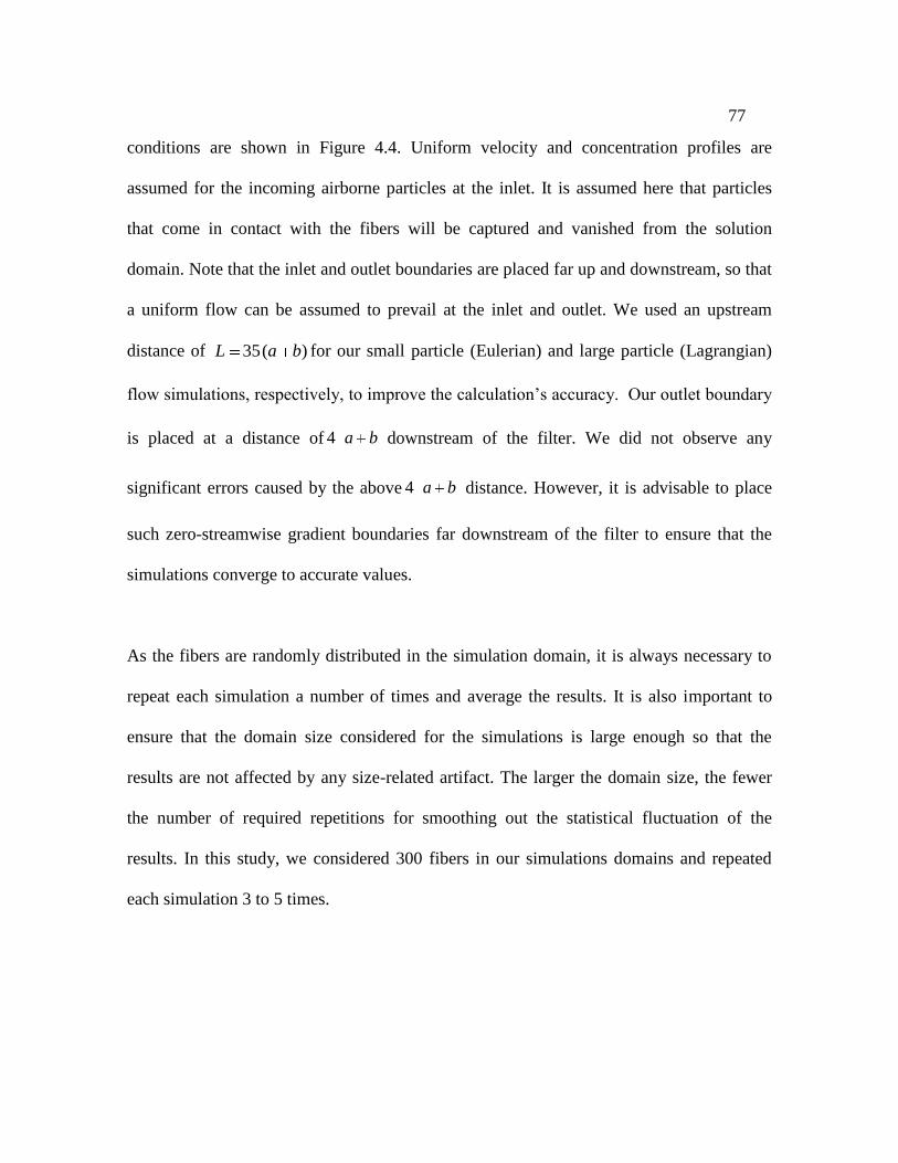
77

conditions are shown in Figure 4.4. Uniform velocity and concentration profiles are

assumed for the incoming airborne particles at the inlet. It is assumed here that particles

that come in contact with the fibers will be captured and vanished from the solution

domain. Note that the inlet and outlet boundaries are placed far up and downstream, so that

a uniform flow can be assumed to prevail at the inlet and outlet. We used an upstream

distance of 35( )L a b for our small particle (Eulerian) and large particle (Lagrangian)

flow simulations, respectively, to improve the calculation’s accuracy. Our outlet boundary

is placed at a distance of 4 a b downstream of the filter. We did not observe any

significant errors caused by the above 4 a b distance. However, it is advisable to place

such zero-streamwise gradient boundaries far downstream of the filter to ensure that the

simulations converge to accurate values.

As the fibers are randomly distributed in the simulation domain, it is always necessary to

repeat each simulation a number of times and average the results. It is also important to

ensure that the domain size considered for the simulations is large enough so that the

results are not affected by any size-related artifact. The larger the domain size, the fewer

the number of required repetitions for smoothing out the statistical fluctuation of the

results. In this study, we considered 300 fibers in our simulations domains and repeated

each simulation 3 to 5 times.

78

Symmetry boundary conditions are considered for the upper and lower boundaries of the

domain, i.e., the gradient of flow properties (velocity, particle concentration …) is zero at

these boundaries. The general problem with symmetry boundary condition is that it does

not allow lateral flow to take place. However, for large simulation domains, like those

considered here, this should not be a concern as the net flow in the lateral directions will

average to zero.

Standard Discrete Phase Model (DPM) in the ANSYS code ignores the dimensions of the

particle during trajectory tracking. Collision between a particle and a wall boundary is

considered to be the moment that the particle center of mass touches the wall boundary,

which obviously is not realistic. In this work, we developed a UDF to instruct ANSYS to

stop the particle if it comes in one radius distance from the wall boundary, as mentioned

previously. This has been done by continuously monitoring the distance between the

particles’ centers and fibers’ surface during the trajectory tracking. If the particle’s center

of mass reaches a distance of away from a fiber, it will be counted as deposited. Note that

for the Lagrangian particle tracking, symmetry boundary conditions act like a perfectly

reflecting wall, i.e., particles colliding with the symmetry boundaries will be reflected

without any loss of momentum.

Figure 4.5a shows the particle concentration contour plot throughout the domain for a

typical trilobal medium considered in this work. Red to blue represents normalized nano-

particle concentration from 1 to zero. Figure 4.5b depicts the trajectory of particles’ centers

79

of mass for 0.5µm particles in the same solution domain. For the sake of clarity, only a few

particle trajectories are shown. Our filter geometries were meshed with triangular cells in

the filter zone and quadrilateral cells in the fluid entry zones. Depending on the fiber aspect

ratio, 3,000,000 to 7,000,000 cells were used in the simulations presented in this section.

Larger numbers of cells are considered in simulations with greater aspect ratios to correctly

resolve the flow field at shaper corners of high aspect ratio fibers. To find out the

minimum number of mesh points needed to conduct mesh-independent simulations, a

single trilobal fiber was placed in the middle of a square 2-D domain. The sides of the

square were chosen such an SVF of 10% was achieved (see Figure 4.6). The pressure drop

caused by this single fiber was monitored as the number of mesh points per each lobe of

the fiber was increase from 10 to 100. It can be seen that grid density has negligible effect

on the pressure drop prediction for more than 80 grids per lobe.

To correctly predict the particle capture efficiency via interception and impaction, one

must release a large number of particles in the flow domain to ensure that the results are

independent of number of particles at inlet. Figure 4.7 shows the influence of number of

particles introduced at the inlet on the medium’s collection efficiency using the Lagrangian

method (equation 2.10). The horizontal axis here is the number of particles per unit of

length at the inlet ( hN p / ). It can be seen that particle collection efficiency (due to

interception and inertial impaction) is independent of the number density of the particles at

the inlet beyond a value of about 6102 , and so we used this density for the particle

injection at the inlet.

80


4.4.1 Performance of 2-D Micro-Structure

As mentioned before, despite their wide spread applications, trilobal media have not been

systematically studied in the literature. Unfortunately, there are no reliable experimental

studies available in the literature that could be used here for our model validation.

Therefore, we validate our simulation methodology by presenting a comparison between

results of our simulations of circular media with the predictions of some of the available

empirical/semi-empirical models that have been developed for media with circular fibers

(see Section 4.1). Figure 4.8 shows penetration per thickness through filter media with a

SVF of 10% made up of circular fibers with a diameter of 14.9 µm along with the

predictions of the expressions developed by Stechkina and Fucks (1966) and Lee and Liu

(1982). Good agreement between our modeling results and these empirical correlations is

evident especially for particles greater than 200 nm. In this figure, we also included our

simulation results obtained for trilobal media with fibers having an aspect ratio of

2ζ and a minor axis of 2b µm (resulting in a circumscribed diameter of 14.9 9 µm).

The idea of using the circumscribed circle was inspired by the fact that the flow inside a

fibrous medium is highly viscous ( Re 1 ) (i.e., Stokes flow regime), and the presence of

an obstacle (whether trilobal or circular) is sensed by the fluid particles (as well as the solid

nano-particles) far upstream of the fiber (see Figure 4.9). Therefore, streamlines are

deflected far before they are close to the fiber. Deflection of the streamlines is mostly

caused by the projected area of the fibers on a plane normal to the flow direction, rather

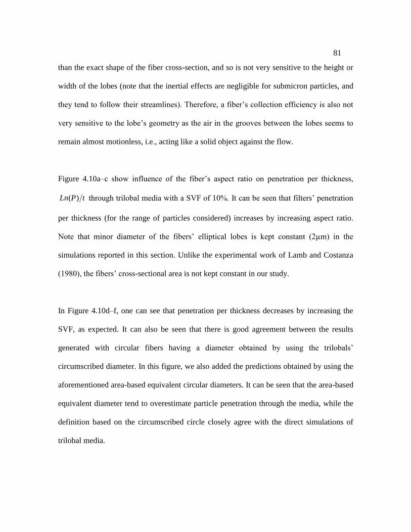
81

than the exact shape of the fiber cross-section, and so is not very sensitive to the height or

width of the lobes (note that the inertial effects are negligible for submicron particles, and

they tend to follow their streamlines). Therefore, a fiber’s collection efficiency is also not

very sensitive to the lobe’s geometry as the air in the grooves between the lobes seems to

remain almost motionless, i.e., acting like a solid object against the flow.

Figure 4.10a–c show influence of the fiber’s aspect ratio on penetration per thickness,

( )Ln P t through trilobal media with a SVF of 10%. It can be seen that filters’ penetration

per thickness (for the range of particles considered) increases by increasing aspect ratio.

Note that minor diameter of the fibers’ elliptical lobes is kept constant (2µm) in the

simulations reported in this section. Unlike the experimental work of Lamb and Costanza

(1980), the fibers’ cross-sectional area is not kept constant in our study.

In Figure 4.10d–f, one can see that penetration per thickness decreases by increasing the

SVF, as expected. It can also be seen that there is good agreement between the results

generated with circular fibers having a diameter obtained by using the trilobals’

circumscribed diameter. In this figure, we also added the predictions obtained by using the

aforementioned area-based equivalent circular diameters. It can be seen that the area-based

equivalent diameter tend to overestimate particle penetration through the media, while the

definition based on the circumscribed circle closely agree with the direct simulations of

trilobal media.

82

The results shown in Figure 4.10 indicate that diameter of the circumscribed circle of a

trilobal fiber can effectively be used to predict collection efficiency of trilobal filters. It

should be noted, however, that using this diameter, SVF of the media increases drastically.

The new SVF helps achieving good predictions for collection efficiency; however, it

results in wrong pressure drop estimates. To solve this problem, we simulated series of

trilobal single fibers in domains similar to the one shown in Figure 4.6, and calculated the

their pressure drops for different SVFs of 5, 6, 7.5, 9 and 10 percent and different aspect

ratios of 1.5, 2, 2.5 and 3. These simulations were then repeated for the circumscribed

equivalent fiber of each trilobal fiber for comparison purposes (see Figure 4.11). In this

figure, each line represents the relationship between pressure drop per thickness of trilobal

filters and their equivalent circumscribed media. Figure 4.11 can be used to predict the

pressure drop of a trilobal medium, tritp , using the pressure drop value of its equivalent

circumscribed medium, cctp , obtained with equations given in section 4.1. For the sake

of convenience, we also presented an equation for each line shown in Figure 4.11. Note

that to calculate cctp , one needs to know the SVF of the equivalent circumscribed

media. Assuming tK to be the ratio of the SVF of the equivalent medium to that of the

original trilobal media, we have:

t cc triK α / α (4.6)

where tri and cc are the SVF of media made of trilobal and circumscribed circles,

respectively. In general, ( )t tK K ζ ,b , where ba / is the fiber aspect ratio. We

calculated tK for different values of1 5b micron and1 5ζ , and plotted the results in

83

Figure 4.12. It can be seen that dependence on b is quite negligible in comparison to that on

the aspect ratio. This allows us to neglect the dependence on b and develop an easy

expression for ( )t tK K ζ , as follows:

36.04.1tK (4.7)

This equation can be used to calculate SVF of the circumscribed circle equivalent media of

each trilobal filter.

In Figure 4.13, we compare pressure drop per thickness of trilobal media and their

equivalent circumscribed media as they were obtained from our CFD simulations. The

media considered here have an aspect ratio of 2, a minor elliptical axis of 2b µm, and

three different SVFs of 5, 7.5, and 10 percent. As explained earlier, pressure drop of the

equivalent media is much higher than that of the actual trilobal filters. These pressure drop

values are then corrected using the relationships given in Figure 4.11 and added to Figure

4.13. It can be seen that corrected the pressure drop values are in good agreement can be

expected values. In this figure we also included the predictions of the analytical model of

Drummond and Tahir (1984) for the equivalent circumscribed media. The good agreement

between our simulation results and the well-known model of Drummond and Tahir (1984)

validates the accuracy of the simulations.

4.4.2 Test Case: Performance of 3-D Micro-Structure

This section is intended to examine whether or not equations and conclusions obtained

from our 2-D simulations are valid for real 3-D filters. In the absence of reliable

experimental data, we use 3-D virtual fibrous structures, as they more realistically

84

represent the micro-structure of a real filter medium Three-dimensional simulations require

extensive computing resources, and so are not suitable for an extensive parameter study.

Here, we use 3-D simulations for validation purposes only. To do so, we generate a few 3-

D fibrous media with trilobal fibers having 1 5ζ a / b . using the Geodict code, and

calculate their pressure drop and collection efficiencies. We then use our circumscribed

equivalent media to predict these results. GeoDict is a voxel-based code developed by

Math and Market, and is validated in many recent publications by other studies (e.g. see

Schulz et al., 2007). To generate the trilobal-shaped fibers, Geodict software uses a special

mathematical formulation for trilobal fibers as presented in Equation 4.8:

0 1

0 1

1 sin 3 cos

1 sin 3 sin

x r r . θ θ

y r r . θ θ (4.8)

Where, 0r and

1r are the constant and θ varies between 0 to 360 degrees. Figure 4.14 shows

three trilobal cross sections with different values of 0.95, 0.35 and 0.2 for1r . It is obvious

that using the Geodict software is not helpful if one wants to study the effects of lobes’

aspect ratio. Therefore, we only picked the geometry with0 7 8r . and the amplitude

of1 0 35r . , which gives the trilobal cross section with identical cross sectional area and

perimeter as our generated geometry. Our voxel size independence has revealed that

consistent results can be obtained from Geodict by using 0.3 µm as the voxel size. Here,

we compare the performance of trilobal media with that of their circumscribed and area-

based equivalent structures (see Figure 4.15). Collection efficiencies of these media are

compared with one another in Figure 4.16. It can be seen that circumscribed equivalent

85

media, unlike the area-based model, can be used to predict the efficiency of trilobal media

with acceptable accuracy. Table 4.1 presents pressure drop per thickness of media shown

in Figure 4.16. We also added the empirical correlation of Davies (1973) for comparison. It

can again be seen that our circumscribed-circle-equivalent model together with its

correction factor can be used to predict the pressure drop of a trilobal medium.

4.4.3 Filters with Star-Shaped Fibers

Here we considered 8-lobe star-shaped fibers. We rotated an ellipse for 45, 90, 135, 180,

225, 270 and 315 degrees around its antipodal point and result is a star-shaped fiber as it

can be seen in Figure 4.17. In this figure, both area-based equivalent circle and

circumscribed circle are shown. Figure 4.18 shows the effect of different aspect ratios on

the performance of star-shaped fibers. In this figure different aspect ratios of 2.5, 3 and 4

with constant SVF of 10% have been considered and the results for penetration per

thickness of media are presented. These results prove that the circumscribed equivalent

diameter is also applicable to star-shaped fibers, as they result in good prediction for the

collection efficiency of star-shaped fibers. More importantly, results of Figure 4.18 also

indicate that smaller aspect ratios lead to better collection efficiencies. In Figure 4.18, we

can also see a comparison between two filters with different SVFs of 5 and 10%, while the

aspect ratio is kept constant at 2.5. In Figure 4.19, each line represents the relationship

between pressure drop per thickness of star-shaped filters and that of their equivalent

circumscribed media. Figure 4.19 can be used to predict the pressure drop of a star-shaped

medium, Δstar

p t , using the pressure drop values of its equivalent circumscribed

86

medium, Δcc

p t . We also obtained curve fitting equations for lines shown in Figure 4.19.

Note that to calculate Δcc

p t , one needs to know the SVF of the equivalent circumscribed

media.

4.5 Conclusion

In this part of the study, for the first time we established a definition for an equivalent

circular fiber that can be used with the traditional filtration correlations (developed for

filters with circular fibers) for predicting collection efficiency of filters made of trilobal

fibers. Our study was conducted in 2-D simulation domains, and due to the lack of suitable

experimental data, validated via 3-D realistic simulations in which fibers random

orientations were taken into account. We demonstrated that the circumscribed circle of

trilobal fibers can be used with the existing traditional empirical/semi-empirical

correlations to predict the performance of a trilobal filter medium. We believe that the

information presented in this chapter can be used by the manufacturers to predict and

optimize performance of their media, and help in reducing the experimental trials before

the actual production process.

87

Table 4.1: Pressure drop of the media shown in Figure 4.15. Prediction of the empirical

correlation of Davies (1973), obtained for media with circular fibers, is also added.

3-D

SVF=10%Trilobal

Circum-

scribed

Area-

based

Davies

(1973)Eqs. in

Figure 10

∆Pave./t

(kPa/m)84.33 109.55 81.11 106.55 78

Std. dev. 6.67 16.67 2.78 - -

4.11

Figure 4.1: a) trilobal fiber, source: http://www.fiberwebfiltration.com/Reemay.cfm, b)

overlapping ellipses forming a trilobal cross-section.

88

Aspect ratio

deq

0 1 2 3 4 5 6 70

20

40

60

80

100b=2, Perimeter based

b=2, Circumscribed circle

b=2, Area based

b=4, Perimeter based

b=4, Circumscribed circle

b=4, Area based

Area-based Circumscribed

Perimeter-based

Figure 4.2: Equivalent circular diameters obtained based on equal surface area and equal

perimeter are compared with the diameter of the circumscribed circle for trilobal fibers

with different aspect ratios and two different minor axes of b=2 and 4 micrometer. It can

be seen that equivalent diameter based on equal perimeter is very close to the diameter of

the circumscribed circle.

89

Calculating size of the domain with

fibers aspect ratio and filter’s SVF

Input total number of trilobal fibers

and filter’s SVF

Create a random position for the center

of fiber

Check for overlaps

with previously

fibers

Save the fiber

Yes

No

Figure 4.3: Our program’s flowchart for generating media with random trilobal fibers.

35(a+b)4(a+b)

Vel

oci

ty i

nle

t

Symmetry

Symmetry

Pre

ssure

outl

et

Figure 4: An example of our simulation domains consisting of 300 trilobal fibers with an

aspect ratio of 1.5 randomly placed in square domain resulting in an SVF of 10%.

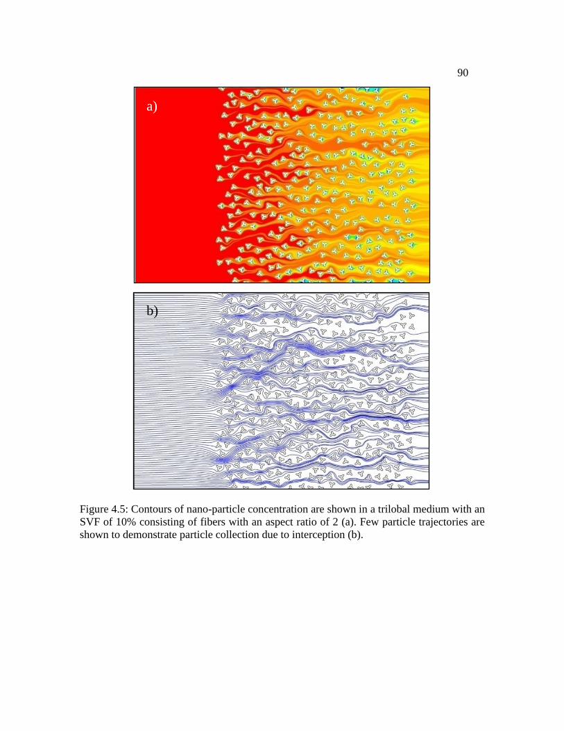
90

a)

b)

Figure 4.5: Contours of nano-particle concentration are shown in a trilobal medium with an

SVF of 10% consisting of fibers with an aspect ratio of 2 (a). Few particle trajectories are

shown to demonstrate particle collection due to interception (b).

91

Number of Mesh per Lobe

Pre

ssure

dro

p(P

a)

0 20 40 60 80 1002.4

2.5

2.6

2.7

2.8

2.9

SVF = 10 %AR = 2

Figure 4.6: Influence of grid density on the pressure drop cause by a single fiber placed in

a domain with an SVF of 10% as shown in the inset.

Particle number density at inlet, NP/h (m

-1)

Ln

(P)/

t(m

-1)

104

105

106

107

-800

-750

-700

-650

-600

-550

-500

-450

SVF = 10 %AR = 2d

P= 1 µm

Figure 4.7: Influence of number of particles injected at the inlet on the penetration

prediction of a typical trilobal media simulated in this study (SVF of 10% and aspect ratio

of 2).

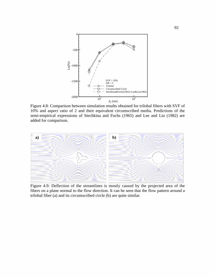
92

dP

(nm)

Ln

(P)/

t

102

103-2000

-1500

-1000

-500

0

Trilobal

Circumscribed Circle

Stechkina&Fuchs(1965)+Lee&Liu(1982)

SVF = 10%AR = 2

Figure 4.8: Comparison between simulation results obtained for trilobal filters with SVF of

10% and aspect ratio of 2 and their equivalent circumscribed media. Predictions of the

semi-empirical expressions of Stechkina and Fuchs (1965) and Lee and Liu (1982) are

added for comparison.

a)

b)

Figure 4.9: Deflection of the streamlines is mostly caused by the projected area of the

fibers on a plane normal to the flow direction. It can be seen that the flow pattern around a

trilobal fiber (a) and its circumscribed circle (b) are quite similar.

93

dP(nm)

Ln

(P)/

t

102

103

-1250

-1000

-750

-500

-250

0

Trilobal

Area-based circle

Circumscribed circle

SVF = 5 %AR = 2

dP(nm)

Ln

(P)/

t

102

103

-1250

-1000

-750

-500

-250

0

Trilobal

Area-based circle


SVF = 7.5 %AR = 2

dP(nm)

Ln

(P)/

t

102

103

-1250

-1000

-750

-500

-250

0

Trilobal

Area-based circle


SVF = 10 %AR = 2

dP(nm)

Ln(P

)/t

102

103

-1500

-1000

-500

0

Trilobal

Area-based circle


SVF = 10 %AR = 1.5

dP(nm)

Ln

(P)/

t

102

103

-1500

-1000

-500

0

Trilobal

Area-based circle


SVF = 10 %AR = 2

dP(nm)

Ln

(P)/

t

102

103

-1500

-1000

-500

0

Trilobal

Area-based circle


SVF = 10 %AR = 3

a)

f)c)

b) e)

d)

Figure 4.10: Penetration per thickness for trilobal media and their equivalent area-based

and circumscribed media at a constant SVF of 10% (figures a–c), and at a constant aspect

ratio of 2 (figures d–f).

94

(Pressure drop / t)cc

(Pa/m)

(Pre

ssu

red

rop

/t)

tri(P

a/m

)

100000 200000 300000 400000 500000

20000

40000

60000

80000

100000

120000

140000

AR = 1.5

AR = 2

AR = 2.5

AR = 3

∆ptri/t =0.6574 ∆pcc/t+7206

∆ptri/t =0.5404 ∆pcc/t+5959

∆ptri/t =0.3997 ∆pcc/t+10911

∆ptri/t =0.3434 ∆pcc/t+13068

Figure 4.11: Relationship between pressure drop of trilobal media and their equivalent

circumscribed equivalents for a SVF of 10% and different aspect ratios of 1.5, 2, 2.5 and 3.

Curve fitting equations are given for each case for convenience.

Aspect Ratio

Kt

1 2 3 4 5

1

2

3

4

5

6

7

991.0

36.04.1

2R

Kt

Figure 4.12: Relationship between SVF of trilobal filters with different aspect ratios and

different minor axis diameter, and those of their circumscribed equivalent media.

95

SVF (%)

Pre

ssure

dro

p/T

hic

knes

s(P

a/m

)

5 6 7 8 9 10

50000

100000

150000

200000

Trilobal


Drummond & Tahir (1984)

Circumscribed circle-modified

Figure 4.13: Pressure drop per thickness for trilobal filters and their circumscribed

equivalent media before and after pressure correction.

3 2 1 1 2 3

2

1

1

2

3

4

AR=1.05

2 1 1 2

2

1

1

2

3

AR=1.5

2 1 1 2

1

1

2AR=5

1 0 95r . 1 0 35r .

1 0 2r .

Figure 4.14: Trilobal fibers with different 1r values created with the mathematical

formulation which is used by Geodict software.

96

a)

x y

z

b)

x y

z

c)

x y

z

Figure 4.15: Three dimensional fibrous media with trilobal fibers having an aspect ratio of

1.5 and an SVF of 10% (a) and, circumscribed (b) and area-based equivalent media (c).

97

dP(nm)

Fo

M

102

103

0.005

0.01

0.015

Trilobal

Area-based circle

SVF = 10 %AR = 1.5

dP(nm)

Ln

(P)/

t

102

103

-1200

-1000

-800

-600

-400

Trilobal

Area-based circle


SVF = 10 %AR = 1.5

(a)

(b)

Figure 4.16: (a) Penetration per thickness and, (b) FOM calculated for the media shown in

the previous figure.


Area-based

circle Figure 4.17: Star-shape fibers

98

dP(nm)

-Ln

(P)/

t

102

103

-400

-350

-300

-250

-200

-150

-100

-50

Star_shaped, AR=3


SVF = 10%

dP(nm)

-Ln

(P)/

t

102

103

-300

-250

-200

-150

-100

-50

Star_shaped, AR=4


SVF = 10%

dP(nm)

-Ln

(P)/

t

102

103

-400

-350

-300

-250

-200

-150

-100

-50

Star_shaped, AR=2.5


SVF = 10 %

dP(nm)

-Ln

(P)/

t

102

103

-150

-100

-50

0

Star_shaped, AR=2.5


SVF = 5 %

dP(nm)

-Ln

(P)/

t

102

103

-400

-350

-300

-250

-200

-150

-100

-50

Star_shaped, AR=3


SVF = 10%

dP(nm)

-Ln

(P)/

t

102

103

-300

-250

-200

-150

-100

-50

Star_shaped, AR=4


SVF = 10%

dP(nm)

-Ln

(P)/

t

102

103

-400

-350

-300

-250

-200

-150

-100

-50

Star_shaped, AR=2.5


SVF = 10 %

dP(nm)

-Ln

(P)/

t

102

103

-150

-100

-50

0

Star_shaped, AR=2.5


SVF = 5 %

dP(nm)

-Ln

(P)/

t

102

103

-400

-350

-300

-250

-200

-150

-100

-50

Star_shaped, AR=3


SVF = 10%

dP(nm)

-Ln

(P)/

t

102

103

-300

-250

-200

-150

-100

-50

Star_shaped, AR=4


SVF = 10%

dP(nm)

-Ln

(P)/

t

102

103

-400

-350

-300

-250

-200

-150

-100

-50

Star_shaped, AR=2.5


SVF = 10 %

dP(nm)

-Ln

(P)/

t

102

103

-150

-100

-50

0

Star_shaped, AR=2.5


SVF = 5 %

dP(nm)

-Ln

(P)/

t

102

103

-400

-350

-300

-250

-200

-150

-100

-50

Star_shaped, AR=3


SVF = 10%

dP(nm)

-Ln

(P)/

t

102

103

-300

-250

-200

-150

-100

-50

Star_shaped, AR=4


SVF = 10%

dP(nm)

-Ln

(P)/

t

102

103

-400

-350

-300

-250

-200

-150

-100

-50

Star_shaped, AR=2.5


SVF = 10 %

dP(nm)

-Ln

(P)/

t

102

103

-150

-100

-50

0

Star_shaped, AR=2.5


SVF = 5 %

(a) (c)

(b) (d)

Figure 4.18: Penetration of star-shaped fibers and their equivalent circumscribed.

(Pressure drop / t)cc

(Pa/m)

(Pre

ssure

dro

p/

t)st

ar(P

a/m

)

0 50000 1000000

20000

40000

60000

AR = 2.5

AR = 3

AR = 4

∆p star /t = 0.8240 ∆pcc /t + 1844

∆p star /t = 0.8015 ∆pcc /t + 1036

∆p star /t = 0.7476 ∆pcc /t + 1732

Figure 4.19: Relationship between pressure drop of star-shaped media and their equivalent

circumscribed.

99

CHAPTER 5 Macro-Scale Modeling of Pleated Surface Filters

5.1 Introduction

Almost all existing theories of aerosol filtration are developed for flat media placed

perpendicular to the air flow direction. These theories have resulted in a series of semi-

analytical expressions derived for calculating filter collection efficiency and pressure drop,

which have been widely used to design flat panel air filters. Most filters, however, are

made of pleated media. Expressions for flat filters do not provide any information directly

useful for designing pleated ones. Most of the progress made in developing pleated media

has therefore been based on empiricism.

Pressure drop across a pleated filter is caused by two equally important factors. The first

and most obvious contributor in the filter’s pressure drop is the fibrous medium. The

second contributing factor is the pleat geometry. In a pioneering work, Chen et al. (1995)

modeled the pressure drop across clean filters with rectangular pleats using a finite element

method and discussed the influence of the above factors in a filter’s total pressure drop.

These authors also showed that increasing the pleat count increases the pressure drop due

Contents of this section have been published in an article entitled “Modeling Instantaneous Pressure Drop

of Pleated Thin Filter Media during Dust Loading” by S. Fotovati, S.A. Hosseini, H. Vahedi Tafreshi, and B.

Pourdeyhimi, Chemical Engineering Science, 66 (18), 4036–4046, 2011.

100

to the geometry but decreases that caused by the fibrous media. Therefore, there exists an

optimum pleat count at which the total pressure drop of a clean pleated filter is a minimum.

To the knowledge of the authors, there are only very few studies in the literature dedicated

to studying the influence of pleat geometry, and almost all of them neglect the effects of

dust deposition on pressure drop (Chen et al., 1995; Lucke and Fissan, 1996; Del Fabbro et

al., 2002; Caesar and Schroth, 2002; Subernat et al., 2003; Tronville and Sala, 2003;

Wakeman et al., 2005; Waghode et al., 2007; Lo et al., 2010; and Rebai et al., 2010). Dust

deposition can adversely affect the performance of a filter over time, and surprisingly, it

has not yet been included in the theories developed for filter design. Therefore, the

objective of our current study is to investigate the influence of particle deposition on the

rate of pressure drop increase in filters with different pleat geometries.

5.2 Pleated Geometry and Flow Field

In this study, we assume the fibrous media to be highly efficient like those used in HEPA

filters. Such media usually have a layered micro-structure with relatively low permeability.

Normally, dust particles (i.e., large particles with a diameter greater than 2-3 microns)

cannot penetrate through such filters. Consequentially, most of the particles deposit on the

surface of the fibrous media leading to the formation of a surface cake. Our study here is

aimed at modeling such filters. We performed a series of simulations to model filters

having rectangular (U-shaped) or triangular (V-shaped) pleats with different widths or

angles, respectively (see Figure 5.1). The geometric parameters are the pleat height L and

pleat width d (or pleat angle 2θ ). Another important parameter is the face velocity, which

101

is the flow velocity when it enters the fibrous media, medium and should not be confused

with inlet velocity, which is the flow velocity as it inters the filter (see Figure 5.1).

Unlike previous chapters, in this part of the study we are dealing with Navier-Stokes

equation and the convective terms are not negligible anymore. The governing equations for

the flow of air a pleated geometry are:

0u v

x y (5.1)

and

2 2

2 2( )

u u p u uu v

x y x x y (5.2-1)

2 2

2 2( )

v v p v vu v

x y y x y (5.2-2)

Governing equations for the air flow inside the fibrous media is the same as those shown in

Equations 5.1–5.2, except for the convective terms on the left hand side of the equations,

which will be negligible for flow in dense porous medium. In fact the filter media in our

work is modeled like a porous material with a given permeability tensor. As mentioned

earlier, most high-efficiency filter media have layered micro-structures, i.e., fibers that do

not have any significant through-plane orientations. In such media, the in-plane and

through-plane permeability constants are quite different from one another (see Tahir and

Tafreshi, 2009 and Fotovati et al., 2010 for more information). Spielman and Goren (1968)

proposed the following expressions for the in-plane and through-plane permeability of

layered media as we presented them in Table 1.1b (Equations 1.19 and 1.20). For

102

completeness of the study, we have also modeled pleated filters with three-dimensionally

isotropic fibrous structures. The expression of Spielman and Goren (1968) for 3-D

isotropic fibrous media is given as Equation 1.21 in Table 1.1b. This information is fed

into the ANSYS CFD code for simulating the pressure drop across pleated media. Due to

the inherent symmetry of the pleated geometries, we only considered one pair of pleats

bounded by symmetry boundary conditions (see Figure 5.1).

5.3 Modeling Dust Deposition

Unlike previous studies reported in the literature, our objective here is to simulate the

effects of pleat geometry on the dust cake formation and its effects on the pressure drop.

As dust particles are a few micrometers in diameter, they cannot normally penetrate a high-

efficiency filter. Therefore, it is reasonable to assume that dust particles will only deposit

on the surface of filter media. To model the deposition of dust particles on a filter surface,

we used the Lagrangian particle tracking method. In this method, each individual particle

is tracked throughout the simulation domain, and their positions are recorded once they are

deposited. In the Lagrangian method, the force balance on a given particle is integrated to

obtain the particle position at a given time. The dominant force acting on a particle is the

air drag force and it can be modeled with the equation we introduced in previous chapters

(Equation 2.10).

Previously, it has been mentioned that ANSYS treats a particle as a point mass and

therefore cannot calculate the particle deposition due to interception. We have addressed

103

this problem by defining a User Defined Function (UDF) that modifies ANSYS’s standard

particle tracking scheme to include the particle deposition via interception. In fact, if a

particle’s center of mass reaches a distance from the filter surface equal to its radius, it will

be counted as deposited. We created another UDF to make ANSYS recognize any particle

whose center reaches one diameter away from the center of any deposited particle, and

considers it to be captured as well. To simulate caking, we repeatedly injected batches of

randomly positioned particles from the inlet until a dust cake was formed. In our

simulations, we injected 160 batches of particles (each batch representing a pseudo time

step). To ensure the realistic randomness of the cakes, particles should be injected from

random positions on the inlet. This was accomplished by developing a UDF to enhance

ANSYS’s standard discrete phase module.

A User Defined Memory (UDM) value has been assigned to each marked cell (i.e., the cell

containing one or more deposited particles) in order to calculate its solid volume fraction.

If the solid volume fraction of a cell increased to a certain value, then the cell was

considered full and no other particle was allowed to enter that cell. In addition, the

permeability of that cell was decreased, which meant that this cell was a part of the dust

cake medium. An additional UDF has been developed to check the UDM value of each and

every cell in the domain, and to assign a permeability value (the cake’s permeability

constant) to them, if considered fully occupied. The cake permeability value was

approximated using the Kozeny- Carman expression (Dullien, 1991):

104

2 3

2180 1

p

KC

dk (5.3)

As it can be seen in the above equation, permeability of a granular cake strongly depends

on its porosity. Determining porosity of the cakes formed by deposition of dust particles on

the surface of a filter is a challenging task. However, there are a few studies in the

literature that report estimated values for porosity of cakes made up of different particle

diameters (Hoffmann and Finkers, 1995, Yu et al., 1997, Thomas et al., 2001, Kasper et

al., 2010). Here, we used the porosity values reported by Kasper et al (2010). As will be

discussed in the next section, porosity values of 65% and 85% have been considered for

cakes made of particles with diameters of 10µm and 3µm, respectively. With these cell

permeability values, the flow field was recalculated and the pressure drop values were

reported after each particle deposition.


As mentioned earlier, we considered rectangular (U-shaped) and triangular (V-shaped)

pleat shapes with different dimensions, and simulated their pressure drop with and without

dust load. We assumed a constant pleat height of 25.4 mm (1 in.), and the medium

thickness of 0.38 mm. For the rectangular and triangular pleats, we considered pleat counts

of 3, 4, 5, 7, 10, 15 and 20 pleats per inch and pleat angles of ( in Figure 5.1) 2, 4, 5, 8, 10,

15 and 20 degrees, respectively. We also used two inlet velocities of 0.2 m/s and 1.0 m/s,

and two dust particle diameters of 3µm and 10µm. With a constant thickness, we

arbitrarily chose different fiber diameters, porosities, and fiber orientations to simulate

105

different filter media with low (F1 and F4), medium (F2 and F5), and high (F3 and F6)

permeability constants (see Table 5.1).

5.4.1 Pressure Drop across Clean Pleated Filters

In this section, we discuss the effect of pleat count on pressure drop in the absence of dust

particle deposition (clean filters). As mentioned earlier, the total pressure drop across a

pleated filter can be attributed to the pressure drop caused by the fibrous media and that

brought about by the pleat geometry. For instance, increasing the pleat count (decreasing

the pleat width or angle) increases the geometry-induce pressure drop, while it reduces the

media-induced pressure drop. The latter is due to the fact that increasing the number of

pleats increases the total filtration surface, and so decreases the face velocity. A decreased

face velocity obviously results in a lower media-induced pressure drop. Similarly,

decreasing the number of pleats reduces the geometry-induced pressure drop and lead to

higher media-induced resistivity.

Figures 5.2a–b show the predicted pressure drop values for different U-shaped pleats at

two different air speeds of 0.2 and 1 m/s, respectively. Figure 5.2c– d show similar results

for V-shaped pleats. The filter media considered for these simulations are those shown in

Table 5.1 (F1, F2, and F3). The optimum pleat count for our U-shaped pleats seems to be

around 5 pleats per inch for the filter media with high permeability. The optimum pleat

count tends to shift towards larger values when the filter media is less permeable. Similarly

with the V-shaped pleats, our results indicate that with the highly permeable media, the

106

minimum pressure drop occurs at a pleat angle of about 10 to 15 degrees, and it moves

towards smaller pleat angles (larger pleat counts) by decreasing the medium’s

permeability. For the range of air velocities considered in this study, the influence of inlet

velocity on the optimum pleat count seems to be minor.

For the completeness of our study, we have also simulated the pressure drop for pleated

filters with three-dimensionally isotropic fibrous structure (F4, F5, and F6). Note that most

high-efficiency filter media have layered micro-structures similar to those of F1, F2, and

F3. Three-dimensionally isotropic media are only considered here to investigate whether or

not the fiber orientation and the media’s anisotropy have any significant influence on the

pressure drop of pleated filters or their optimum pleat counts. Interestingly, our results

indicate that isotropic media produce smaller pressure drop values compared with their

layered counterparts (see Figure 5.3). This is believed to be due to the fact that, for the

same fiber diameter and solid volume fraction, permeability of a layered media in the

through-plane direction is lower than that of a three-dimensionally isotropic media. Note

that, as will be discussed in the next subsections, air enters the media at a normal angle,

regardless of the pleat count (or angle) or flow velocity, and so the only component of the

permeability tensor that plays a dominant role becomes the through-plane component (see

Figures 5.4–5.6).

107

5.4.2 Dust Particle Deposition Pattern

To simulate deposition of dust particles, batches of particles were injected from the inlet

over the course of several “time steps”. Aerosol concentration was assumed to be 132 10

particles per cubic meter. Flow field throughout the domain was recalculated after

deposition of each batch of particles (each time step), and pressure drop was recorded. As

dust load simulations are CPU intensive in nature, we only considered the second fibrous

medium from Table 1, i.e., F2, for our dust-loaded filter simulations.

Figure 5.4 shows the dust distribution and flow streamlines inside different rectangular and

triangular pleats. Particle diameter and flow velocity at the inlet are 3µm and 0.2 m/s,

respectively. Figures 5.4a and 5.4c show that the dust cake covers all available filtration

surfaces quite uniformly for the geometries with small pleat counts. With higher pleat

counts (Figures 5.4b and 5.4d), some small dendrites are formed inside the pleats,

especially with the U-shaped pleats.

Figure 5.5a and 5.5b show the dust pattern and flow streamlines inside the U-shaped pleats

with 4 and 20 pleats per inch, respectively. In these simulations particle size to 10µm but

the flow velocity is the same as that of Figure 5.4. Simulations for the V-shaped pleats for

pleat angles of o15 and o4 are shown in Figure 5.5c and 5.5d, respectively. These results

indicate that while the dust distribution is still somewhat uniform for wide pleats (low pleat

counts either rectangular or triangular), increasing the pleat count increases the chance of

tall dendrite growth, which is the case with the geometry shown in Figure 5.5b. Also, note

108

that in the case shown in Figure 5.5b, particles tend to travel deeper inside the pleat

channels due to their considerable mass, leaving a noticeably clean surface near the pleat

entrance. This happens because larger particles cannot perfectly follow their streamlines at

the sharp 90-degree turn at the pleat entrance, and migrate to the center of the channel.

Obviously, this effect is less pronounced with triangular pleats as the turn at the pleat inlet

is milder.

The same simulations as discussed above are repeated with particles having a diameter of

10µm and the flow having a speed of 1.0 m/s (see Figure 5.6). Particles with a diameter of

10µm and a speed of 1.0 m/s have considerable inertia and tend to travel on straight lines,

rather than following their streamlines when encountering a deposited particle (or a sudden

turn). Consequently, if they come in contact with any deposited particle, the contact point

is most probably on the upstream side of the previously deposited particles. It is interesting

to note that, especially in Figure 5.6(a–b), dendrites tend to grow upstream against the flow

direction, and even formed a “bridge” over some part of the filter media near the inlet

(Figure 5.6a). Note also that for the pleat shown in Figure 5.6b the cake has moved deep

inside the pleat. Results of Figure 5.6 reveals that with high-inertia particles, even in the

case of small number of pleats one can observe non-uniform dust cake formation. Note

again that the dust deposition pattern in the V-shaped pleats is more uniform than that in

the U-shape pleats.

109

A higher pleat count results in a lower face velocity for a constant pleat height (Chen et al.,

2008, and Chen et al., 1995). This is due to the fact that with higher number of pleats the

filtration surface is larger, and for a constant flow rate through the filter, the face velocity

is inversely proportional to surface area. However, more pleat count leads to the formation

of narrower channels for the flow. The streamwise velocity through a pleat must be higher

when less mass is leaving the channel walls as a result of a higher pleat count inducing a

lower face velocity. Flow velocity averaged over the pleat’s centerline path is reported in

Figures 5.7a and 5.7b for rectangular and triangular pleats, respectively. As expected,

centerline velocity increases with increasing the pleat count or decreasing the pleat angle.

Because of this effect with higher pleat counts, i.e., higher streamwise and lower lateral

velocities, particles tend to travel on straight line and deposit deeper inside the pleat.

For further analysis, we provided the particles’ mass distribution along the x-direction over

the pleats. Figure 5.8 shows the deposited mass along the x-coordinate inside U-shaped

and V-shaped pleats for different flow velocities of 0.2 and 1 m/s and particle diameters of

3 and 10 µm. Mass of the deposited particles is give in an arbitrary unit as it is simply the

number of cells in the domain which are occupied with particles. As can be seen, with

lower pleat counts and at lower flow velocities, particles tend to cover the entire surface of

the pleats. Figures 5.8c and 5.8f quantitatively show the above observation that high-inertia

particles tend to deposit deep inside the pleats when the pleat count is high.

110

5.4.3 Effects of Dust Deposition on Pressure Drop

In the previous subsections we showed how different particle sizes and different flow

speeds come into account and discussed how they may affect dust deposition for different

pleat geometries. In this section we investigate the resultant effects on a filter pressure

drop. In particular, here we discuss how a filter pressure drop changes with respect to its

unloaded pressure drop. To minimize the statistical errors associated with random particle

injection and therefore random cake formation, we repeated each of our simulations up to

three times and averaged the results.

Figure 5.9 shows the pressure drop increase during particle loading in different rectangular

and triangular pleats at different air inlet speeds of 0.2 and 1 m/s. It can be seen that except

for the very early stages of loading, pressure drop increases almost linearly with increasing

the number of deposited particles (or time), especially when the air velocity is relatively

slow (i.e., 0.2 m/s). Obviously, the non-linearity in the pressure drop increase shown in

Figures 5.9e and 5.9f must be attributed to the non-uniform dust deposition inside the

pleats at an air velocity of 1 m/s, as discussed earlier. Interestingly, the rate of pressure

drop increase is higher with low pleat counts. In other words, increasing the number of

pleats greatly helps lowering the rate of increase of pressure drop during particle loading.

This is in contrast to the case of clean filters where there exists an optimum pleat count at

which the pressure drop is a minimum. Note that the final pressure drop is higher for larger

particles when the air velocity is kept constant (see Figures 5.9a–d). This is because

porosity of a cake made up of 10µm particles is less than the cake made of 3µm particles,

111

which leads to a lower permeability for former. When the air velocity is higher pressure

drop increase is less (see Figures 9c–f), which is most probably due to the non-uniformity

of the dust load. When the dust cake is not distributed uniformly over the filter media,

there are places where cake thickness is very thin or there is no dust at all. This allows air

to find the path of minimum resistance and flow through the filter with minimum pressure

drop.

5.4.4 Effects of Cake Permeability on the Optimal Pleat Count

The results discussed so far indicated that for the range of particle diameters and air

velocities considered, a higher pleat count results in a smaller rate of pressure drop

increase caused by particle loading. It should be noted that this conclusion depends on the

cake permeability relative to the filter media. Permeability of a granular medium (i.e., dust

cake) is normally one or two orders of magnitude lower than that of a fibrous medium.

This is mostly because granular beds pack denser than fibrous beds. It is informative here

to investigate if a higher pleat count still causes a smaller rate of pressure drop increase if

the dust cake is more permeable than the filter media. To do so, we assumed a highly

porous dust cake with a porosity of 92.5% made up of particles with a diameter of 10µm.

This cake is three times more permeable than the fibrous medium of the filter. Results of

these simulations, conducted with an air velocity of 0.2m/s, are given in Figure 5.10. It can

be seen that increasing the number of pleats does not result in lowering the rate of pressure

drop increase. As the fibrous medium is the most resistive element in such a condition,

non-uniform dust deposition does not necessary help with lowering the pressure drop. As

112

shown in the latter figure, one may still be able to find an optimum pleat count if the cake

permeability is higher than the filer media.

5.4.5 A Comparison between Rectangular and Triangular Pleats

The rectangular and triangular pleat geometries discussed in the past sections did not

necessarily have identical pleat counts, and so it was not accurately comment on the

performance of one versus the other. In this section we intend to compare filters having

rectangular and triangular pleats with identical pleat counts. Here we compare performance

of a filter with 15 rectangular pleats per inch with that of a filter with 15 triangular pleats

per inch (pleat angle of o4 ). Since both geometries have the same pleat width ( d ) hence

each injected batch of particles in their corresponding simulation domains includes the

same number of particles. Note that even though both geometries have the same pleat

count, the U-shaped geometry has a slightly more filtration surface area (see Figure 5.1).

The dust distribution and air streamlines inside the above rectangular and triangular pleats

are shown in Figure 5.11 for different air flow velocities of 0.2 and 1 m/s and different

particle diameters of 3 and 10 µm. As can be seen, a uniform dust deposition covers almost

the entire filter surface when the particles are small and the air flow is relatively slow. As

we increase the particle size, non-uniform dendrites begin growing inside the rectangular

pleat (see Figure 5.11b). Eventually, with the large particles and fast air flow, particles

travel deeper inside the channel leaving part of the filtration surface near the pleat entrance

almost clean. This effect is more pronounced with the rectangular pleats. Results of

Figures 5.11 clearly show that dust deposition is more uniform in triangular pleats.

113

Figure 5.12 shows pressure drop increase for U-shaped and V-shaped pleats for different

air flow velocities of 0.2 and 1 m/s, and different particle diameters of 3 and 10 µm. These

results indicate that a dust-loaded filter with rectangular pleats generate significantly

higher pressure drops when compared to its counterpart having triangular pleats, if the

particles are small and air flow is relatively slow (see Figure 5.12a). As the dust particle

diameter increases from 3µm to 10µm, the difference between the above pressure drop

values starts to vanish (see Figure 5.12b). This is believed to be due to the non-uniform

dust distribution in the rectangular pleats as discussed earlier. Surprisingly, by increasing

the air velocity to 1 m/s, an effect opposite of that shown in Figure 5.12a is observed (see

Figure 5.12c). For the high air velocity of 1m/s and the larger particles (10µm), our

simulations indicate a greater rate of pressure drop increase for the triangular pleats.

5.4.6 Effects of Pleat Height on the Performance of the Pleated Filters

It is important to investigate if the effect of pleat height can contribute to dust deposition

pattern. To study this, different triangular geometries with different pleat angles have been

chosen. For each pleat angle, the pleat channel with four different pleat heights has been

considered. In this study only triangular pleats were considered. Six different pleat angles

are considered as 15o, 10

o, 8

o, 5

o, 4

o and 3

o where, pleat heights are equal to 25.4 mm,

20.32 mm, 12.70 mm, and 7.62 mm. The fibrous medium thickness has been kept constant

and the fibrous structure inside the pleated filter for all of simulations is the same as

geometry F2 in Table 5.1. The inlet velocity for all simulations is again a constant value of

0.2 m/s. Dust particles with diameter of 10 µm has been considered.

114

Figure 5.13 shows the clean filter pressure drop for different pleat angles and pleat heights.

As can be seen, with constant angle, shorter pleat height causes more pressure drop. For

larger angles, the flow field is affected mostly because of the medium and because the

pleat angles become smaller.

Figure 5.14a–f shows the velocity profile along the center line of the pleated channels for

all six modeled pleat angles. As can be noticed, with large pleat angle and with longest

pleat height of 25.4 mm, the velocity over the centerline of the channel increases with a

smooth slope and remain almost uniform in most part of the channels. By reducing the

pleat height, the slope increases with faster rate and the maximum velocity happens to be at

the inlet part of the channel. The smallest pleat height of 7.62 mm causes a maximum

velocity at the channel inlet. Moreover, the maximum velocity over the centerline increases

as we decrease the pleat angle when the pleat height is constant. This confirms that

pressure drop due to geometrical effects increases when the pleat height is shorter or pleat

angle is smaller.

The pressure drop due to medium depends only on the face velocity. Face velocity is the

velocity which flow enters the fibrous medium. Figure 5.15(a–f) presents the face velocity

over the filtration surfaces for different pleat angles and heights. For the pleat angle of 15o

(Figure 5.15a), and for the constant pleat height, it can be seen that the face velocity

increases slightly as the flow goes deeper inside the pleated channel. In addition, by

decreasing the pleat height with constant angle, the face velocity increases. The reason is

115

that when the pleat angle is kept constant, the flow rate at the inlet is constant and with

shorter pleat height, the flow has to pass across reduced surface area and hence this causes

more face velocity.

The face velocity profile does not show the uniformity that was observed for large angles

as we decrease the pleat angle and as the pleat angle is reduced, the maximum of face

velocity magnitude shifts toward the beginning parts of the channel (see Figure 5.15f),

while it shows a slight reduction in magnitude as well. The latter perfectly explains why

with smaller pleat heights, large particles tend to deposit deeper inside the pleated

channels. The velocity increase causes inertial particles to move deeper and deposited near

the end of the channels (see Figure 5.16).

Figure 5.17 shows similar results for the smallest pleat angle. A comparison between these

two figures shows that, with larger angle and height, more uniform dust deposition has

been achieved. With the smaller angle, the uniformity is less pronounced in comparison

with other larger angles when the pleat height is 25.40 mm. However, this small uniformity

is somehow lost when the pleat height is getting shorter and shorter. Dust particles are

traveling deeper inside the pleated channel and as can be seen in Figure 5.17d, an unloaded

portion of the filter surface can be observed. Larger dendrites are formed and flow inside

the channel has been affected. In addition, at the site of initial entry into the filter, the

streamlines are no longer perpendicular to the surface of the medium when the either pleat

116

height or pleat angle is reduced. All these effects confirm the fact that shorter pleat heights

increase the geometrical effects.

Pressure drop ratios for different pleat angles and pleat heights are presented in Figure 5.18

(a–f). For relatively large pleat angles (Figures 5.18a–d), it seems that reducing the pleat

height causes a decrease in pressure drop increase ratio, and that the minimum pressure

drop increase happens to be at L= 7.62 mm with the 10 µm dust particles. In contrast, for

very small pleat angles, as can be seen in Figures 5.18e–f, the trend starts to change and the

minimum rate of increase in pressure drop ratio occurs at L= 12.70 mm. This clearly

indicates that, unlike what our previous study showed, for constant pleat height, with

various pleat heights and pleat angles there would be an optimum pleat height at which the

minimum pressure drop increase is the minimum.

5.5 Conclusions

Our simulations, developed for modeling the effects of dust-load on performance of

pleated filters demonstrate that there exists an optimum pleat count for clean filters at

which pressure drop reaches a minimum regardless of the in-plane or through-plane

orientation of the fibers. With the particle deposition included in the analysis, our results

indicated that the rate of increase of pressure drop decreases with increasing the pleat

count. We demonstrated that a higher pleat count results in a higher flow velocity inside

the pleat channels causing more non-uniformity in the dust deposition across the pleat.

Especially when particles are sufficiently large, the dust cake tends to form deeper inside

117

the pleated channel when the pleat count is high. This effect is observed to be less

pronounced when the pleats have a triangular shape. We also showed that if the dust cake

permeability is higher than that of the filters fibrous media, the rate of increase of pressure

drop does not always decrease with increasing the pleat count. Finally, by comparing

filters having 15 pleats per inch, we observed that rectangular pleats are preferred over the

triangular pleats when the particles are highly inertial, i.e., filtering high-speed large

particles. When particle’s inertia is small, our results indicate that triangular pleats cause

less pressure drop, and so are recommended.

118

Table 5.1: Different fibrous media considered for this study.

Filter

media

Fiber

diameter

(µm)

Solid Volume

Fraction

(%)

In-plane

Permeability

(m2)

Through-plane

Permeability

(m2)

Isotropic

Permeability

(m2)

F1 6 102.78 10-11 1.51 10-11 not applicable

F2 10 7.51.22 10-10 7.10 10-11 not applicable

F3 15 46.92 10-10 4.40 10-10 not applicable

F4 6 10 not applicable not applicable2.25 10-11

F5 10 7.5 not applicable not applicable1.01 10-10

F6 15 4 not applicable not applicable5.88 10-10

b) Symmetry

Symmetry

2θ

inle

t

a)

Ld

inle

t

Symmetry

Symmetry

Face velocity

Figure 5.1: Simulation domain for a) rectangular pleats, and b) triangular pleats

119

Pleat count (1/in)

p0

(Pa)

5 10 15 20

5

35

65

95k

TP

lay=1.51x10

-11(m

2) & k

IP

lay=2.78x10

-11(m

2)

kTP

lay=7.10x10

-11(m

2) & k

IP

lay=1.22x10

-10(m

2)

kTP

lay=4.40x10

-10(m

2) & k

IP

lay=6.92x10

-10(m

2)

U-shaped

uin= 0.2 m/s

a)

Pleat angle (deg.)

p0

(Pa)

5 10 15 20

5

25

45

65 kTP

lay=1.51x10

-11(m

2) & k

IP

lay=2.78x10

-11(m

2)

kTP

lay=7.10x10

-11(m

2) & k

IP

lay=1.22x10

-10(m

2)

kTP

lay=4.40x10

-10(m

2) & k

IP

lay=6.92x10

-10(m

2)

V-shaped

uin= 0.2 m/s

c)

Pleat angle (deg.)

p0

(Pa)

5 10 15 20

5

55

105

155

205 kTP

lay=1.51x10

-11(m

2) & k

IP

lay=2.78x10

-11(m

2)

kTP

lay=7.10x10

-11(m

2) & k

IP

lay=1.22x10

-10(m

2)

kTP

lay=4.40x10

-10(m

2) & k

IP

lay=6.92x10

-10(m

2)

V-shaped

uin= 1.0 m/s

d)

Pleat count (1/in)

p0

(Pa)

5 10 15 205

55

105

155

205255305 k

TP

lay=1.51x10

-11(m

2) & k

IP

lay=2.78x10

-11(m

2)

kTP

lay=7.10x10

-11(m

2) & k

IP

lay=1.22x10

-10(m

2)

kTP

lay=4.40x10

-10(m

2) & k

IP

lay=6.92x10

-10(m

2)

U-shaped

uin= 1.0 m/s

b)

Figure 5.2: Pressure drop of clean filters with U-shaped and V-shaped pleats with different

pleat counts at two different air inlet velocities of 0.2 and 1 m/s. The filter media

considered here have layered micro-structures (see Table 5.1).

120

Pleat angle (deg.)

p0

(Pa)

5 10 15 20

5

20

35

50

6580

kiso

=2.25x10-11

(m2)

kiso

=1.01x10-10

(m2)

kiso

=5.88x10-10

(m2)

V-shaped

uin= 1.0 m/s

d)

Pleat count (1/in)

p0

(Pa)

5 10 15 20

5

20

kiso

=2.25x10-11

(m2)

kiso

=1.01x10-10

(m2)

kiso

=5.88x10-10

(m2)

U-shaped

uin= 0.2 m/s

a)

Pleat count (1/in)

p0

(Pa)

5 10 15 205

20

35

50

65

80

kiso

=2.25x10-11

(m2)

kiso

=1.01x10-10

(m2)

kiso

=5.88x10-10

(m2)

U-shaped

uin= 1.0 m/s

b)

Pleat angle (deg.)

p0

(Pa)

5 10 15 20

5

20

kiso

=2.25x10-11

(m2)

kiso

=1.01x10-10

(m2)

kiso

=5.88x10-10

(m2)

V-shaped

uin= 0.2 m/s

c)

Figure 5.3: Pressure drop of clean filters with U-shaped and V-shaped pleats with different

pleat counts at two different air inlet velocities of 0.2 and 1 m/s. The filter media

considered here have three-dimensionally isotropic micro-structures (see Table 5.1).

121

a) pleat count =4 plt/in

b) pleat count =20 plt/in

c) pleat count =6 plt/in (2θ =15o)

d) pleat count =15 plt/in (2θ =4o)



o pleat

angle. Particle diameter and flow velocity are 3µm and 0.2 m/s, respectively.

122







o pleat

angle. Particle diameter and flow velocity are 10µm and 0.2 m/s, respectively.

123







o pleat

angle. Particle diameter and flow velocity are 10µm and 1 m/s, respectively.

124

Pleat angle (deg.)

u(m

/s)

5 10 15 20

0.25

0.3

0.35

0.4

Centerline Velocity

V-shaped

uin= 0.2 m/s

Pleat count (1/in)

u(m

/s)

5 10 15 20

0.3

0.4

Centerline Velocity

U-shaped

uin= 0.2 m/s

a)

b)

Figure 5.7: Streamwise velocity magnitude on the centerline of pleat channels for a)

rectangular pleats, b) triangular pleats. The inlet velocity is 0.2 m/s.

125

x (mm)

dep

osi

ted

mas

s(a

.u.)

0 5 10 15 20 25

0

250

500

15o

pleat angle

4o

pleat angle

V-shaped

dp= 10 µm

uin= 0.2 m/s

e)

x (mm)

dep

osi

ted

mas

s(a

.u.)

0 5 10 15 20 25

0

500

1000

1500

4 pleat/in

20 pleat/in

U-shaped

dp= 10 µm

uin= 0.2 m/s

b)

x (mm)

dep

osi

ted

mas

s(a

.u.)

0 5 10 15 20 25

0

250

500

15o

pleat angle

4o

pleat angle

V-shaped

dp= 10 µm

uin= 1.0 m/sf)

x (mm)

dep

osi

ted

mas

s(a

.u.)

0 5 10 15 20 25

0

500

1000

1500

4 pleat/in

20 pleat/in

U-shaped

dp= 10 µm

uin= 1.0 m/s

c)

x (mm)

dep

osi

ted

mas

s(a

.u.)

0 5 10 15 20 25

0

250

500

15o

pleat angle

4o

pleat angle

V-shaped

dp= 3 µm

uin= 0.2 m/s

d)

x (mm)

dep

osi

ted

mas

s(a

.u.)

0 5 10 15 20 25

0

500

1000

1500

4 pleat/in

20 pleat/in

U-shaped

dp= 3 µm

uin= 0.2 m/s

a)

Figure 5.8: Dust cake distribution along the x-direction inside rectangular and triangular

pleat geometries.

126

- - - - --

-- - - - - - - - - - - - - - - - - - - - - - - - - - - - - - - - - -

+ + + + + + + + + + + + + + + + + + + + + + + + + + + + + + + + + + + + + + + + +

Number of time steps

p/

p0

0 50 100 150

2

4

6

8 15o

pleat angle

10o

pleat angle

8o

pleat angle

5o

pleat angle

4o

pleat angle

3o

pleat angle

-

+

V-shaped

dp= 3 µm

b)

uin=0.2 m/s

- - - - --

- - - - - - - - - - - - - - - - - - - - - - - - - - - - - - - - - - -

+ + + + + + + + + + + + + + + + + + + + + + + + + + + + + + + + + + + + + + + + +


p/

p0

0 50 100 1500

10

204 pleat/in

5 pleat/in

7 pleat/in

10 pleat/in

15 pleat/in

20 pleat/in

-

+

U-shaped

dp= 3 µm

a)

uin=0.2 m/s

- - - - --

-- - - - - - - - - - - - - -

- - - -- - -

- - - - - - - - - -- -

-

+ + + + + + + + + + + + + + + + + + + + + + + + + + + + + + + + + + + + + + + + +


p/

p0

0 50 100 1500

10

20

30 4 pleat/in

5 pleat/in

7 pleat/in

10 pleat/in

15 pleat/in

20 pleat/in

-

+

U-shaped

dp= 10 µm

c)

uin=0.2 m/s

- - - - - --

- - - - - - - - - - - - - - - - - - - - - - - - - - - - - - - - - -

+ + + + + + + + + + + + + + + + + + + + + + + + + + + + + + + + + + + + + + + + +


p/

p0

0 50 100 1500

5

10

15o

pleat angle

10o

pleat angle

8o

pleat angle

5o

pleat angle

4o

pleat angle

3o

pleat angle

-

+

V-shaped

dp= 10 µm

d)

uin=0.2 m/s

- - - - - - - - - - - - - - - - - - - - - - - - - - - - - - - - - - - - - - - - -

+ + + + + + + + + + + + + + + + + + + + + + + + + + + + + + + + + + + + + + + + +


p/

p0

0 50 100 150

2

4

6

84 pleat/in

5 pleat/in

7 pleat/in

10 pleat/in

15 pleat/in

20 pleat/in

-

+

U-shaped

dp= 10 µm

e)

uin=1 m/s

- - - - --

--

--

--

-- - - - - - - - - - - - - - - - - - - - - - - - - - - -

+ + + + + + + + + + + + + + + + + + + + + + + + + + + + + + + + + + + + + + + + +


p/

p0

0 50 100 150

1

2

3

15o

pleat angle

10o

pleat angle

8o

pleat angle

5o

pleat angle

4o

pleat angle

3o

pleat angle

-

+

V-shaped

dp= 10 µm

f)

uin=1 m/s


pleats for particles with pd of 3 and 10µm and inlet velocities of 0.2 and 1m/s.

127

- - - - - - - - - - - - - - - - - - - - - - - - - - - - - - - - - - - - --

--

-

+ + + + + ++ + + + + + + + + + + + +

++ + +

++

++

++

++

++

++

++

++

++


p/

p0

0 50 100 150

1

1.1

1.2

15o

pleat angle

10o

pleat angle

8o

pleat angle

5o

pleat angle

4o

pleat angle

3o

pleat angle

-

+

V-shaped

dp= 10 µm

- - - - - - - - - - - - - - - - - - - - - - - - - - - - - - - - - - - - - - - - -

+ + + + + + + + + + + + + + + + + + + + + + + + + + ++ + + + + +

++

++

++

++


p/

p0

0 50 100 150

1

1.2

1.4

1.6

4 pleat/in

5 pleat/in

7 pleat/in

10 pleat/in

15 pleat/in

20 pleat/in

-

+

U-shaped

dp= 10 µm

a)

b)

uin=0.2 m/s

uin=0.2 m/s


pleats. The dust cake is assumed to be three times more permeable than the fibrous media.

128

b) dp= 10µm, uin= 0.2 m/s

c) dp= 10µm, uin= 1.0 m/s

a) dp= 3µm, uin= 0.2 m/s

Figure 5.11: Dust cake deposition pattern and air streamlines inside filters with 15

rectangular or triangular pleats per inch loaded with particles having 3 and 10µm diameters

with air velocities of 0.2 and 1 m/s.

129


p/

p0

0 50 100 150

1

2

3

4

5

U-shaped, 15 pleat/in

V-shaped, 4o

pleat angle

dp= 3 µm

uin= 0.2 m/s

a)


p/

p0

0 50 100 150

1

2

3

4

5

U-shaped, 15 pleat/in

V-shaped, 4o

pleat angle

dp= 10 µm

uin= 0.2 m/s

b)


p/

p0

0 50 100 150

1

1.2

1.4

1.6U-shaped, 15 pleat/in

V-shaped, 4o

pleat angle

dp= 10 µm

uin= 1.0 m/sc)

Figure 5.12: Comparison between the pressure drop increase for filters with 15 rectangular

and triangular pleats per inch loaded with particles having 3 and 10µm diameters with air

velocities of 0.2 and 1 m/s.

130

Pleat height (mm)

p0

10 15 20 25

2

3

4

5 Pleat angle = 15o

Pleat angle = 10o

Pleat angle = 8o

Pleat angle = 5o

Pleat angle = 4o

Pleat angle = 3o

Figure 5.13: Clean filter pressure drop for pleat angles of 15o, 10

o, 8

o, 5

o, 4

o and 3

o,

regarding to different pleat heights.

131

x (mm)

uce

nte

r(m

/s)

0 0.01 0.02 0.03

0

0.1

0.2

0.3

0.4Pleat heigth = 25.40 mm.

Pleat heigth = 20.32 mm.



2 = 15o

uin= 0.2 m/s

(a)

x (mm)

uce

nte

r(m

/s)

0 0.01 0.02 0.03

0

0.1

0.2

0.3

0.4





2 = 10o

uin= 0.2 m/s

(b)

x (mm)

uce

nte

r(m

/s)

0 0.01 0.02 0.03

0

0.1

0.2

0.3

0.4





2 = 8o

uin= 0.2 m/s

(c)

x (mm)

uce

nte

r(m

/s)

0 0.01 0.02 0.03

0

0.1

0.2

0.3

0.4

0.5





2 = 5o

uin= 0.2 m/s

(d)

x (mm)

uce

nte

r(m

/s)

0 0.01 0.02 0.03

0

0.1

0.2

0.3

0.4

0.5

0.6





2 = 4o

uin= 0.2 m/s

(e)

x (mm)

uce

nte

r(m

/s)

0 0.01 0.02 0.03

0

0.1

0.2

0.3

0.4

0.5

0.6

0.7 Pleat heigth = 25.40 mm.




2 = 3o

uin= 0.2 m/s

(f)

(a)

(b)

(c)

(d)

(e)

(f)

x (mm)

uce

nte

r(m

/s)

0 0.01 0.02 0.03

0

0.1

0.2

0.3





2 = 15o

uin= 0.2 m/s

(a)

x (mm)

uce

nte

r(m

/s)

0 0.01 0.02 0.03

0

0.1

0.2

0.3

0.4





2 = 10o

uin= 0.2 m/s

(b)

x (mm)

uce

nte

r(m

/s)

0 0.01 0.02 0.03

0

0.1

0.2

0.3

0.4





2 = 8o

uin= 0.2 m/s

(c)

x (mm)

uce

nte

r(m

/s)

0 0.01 0.02 0.03

0

0.1

0.2

0.3

0.4

0.5





2 = 5o

uin= 0.2 m/s

(d)

x (mm)

uce

nte

r(m

/s)

0 0.01 0.02 0.03

0

0.1

0.2

0.3

0.4

0.5

0.6





2 = 4o

uin= 0.2 m/s

(e)

x (mm)

uce

nte

r(m

/s)

0 0.01 0.02 0.03

0

0.1

0.2

0.3

0.4

0.5

0.6





2 = 3o

uin= 0.2 m/s

(f)

(a)

(b)

(c)

(d)

(e)

(f)

x (mm)

uce

nte

r(m

/s)

0 0.01 0.02 0.03

0

0.1

0.2

0.3





2 = 15o

uin= 0.2 m/s

(a)

x (mm)

uce

nte

r(m

/s)

0 0.01 0.02 0.03

0

0.1

0.2

0.3

0.4





2 = 10o

uin= 0.2 m/s

(b)

x (mm)

uce

nte

r(m

/s)

0 0.01 0.02 0.03

0

0.1

0.2

0.3

0.4





2 = 8o

uin= 0.2 m/s

(c)

x (mm)

uce

nte

r(m

/s)

0 0.01 0.02 0.03

0

0.1

0.2

0.3

0.4

0.5





2 = 5o

uin= 0.2 m/s

(d)

x (mm)

uce

nte

r(m

/s)

0 0.01 0.02 0.03

0

0.1

0.2

0.3

0.4

0.5

0.6





2 = 4o

uin= 0.2 m/s

(e)

x (mm)

uce

nte

r(m

/s)

0 0.01 0.02 0.03

0

0.1

0.2

0.3

0.4

0.5

0.6





2 = 3o

uin= 0.2 m/s

(f)

(a)

(b)

(c)

(d)

(e)

(f)

Figure 5.14: Clean filter centerline velocity profile for pleat angles of 15o, 10

o, 8

o, 5

o, 4

o

and 3o for different pleat heights.

132

x (mm)

Vfa

ce(m

/s)

0 0.005 0.01 0.015 0.02 0.0250.01

0.02

0.03

0.04

0.05

0.06

Pleat height = 25.40 mm




Pleat angle = 15o

uin= 0.2 m/s

(a)

x (mm)

Vfa

ce(m

/s)

0 0.005 0.01 0.015 0.02 0.025

0.02

0.04

0.06 Pleat height = 25.40 mm




Pleat angle = 5o

uin= 0.2 m/s

(d)

x (mm)

Vfa

ce(m

/s)

0 0.005 0.01 0.015 0.02 0.0250.01

0.02

0.03

0.04

0.05





Pleat angle = 10o

uin= 0.2 m/s

(b)

x (mm)

Vfa

ce(m

/s)

0 0.005 0.01 0.015 0.02 0.025

0.02

0.04

0.06Pleat height = 25.40 mm




Pleat angle = 4o

uin= 0.2 m/s

(e)

x (mm)

Vfa

ce(m

/s)

0 0.005 0.01 0.015 0.02 0.0250.01

0.02

0.03

0.04

0.05





Pleat angle = 8o

uin= 0.2 m/s

(c)

x (mm)

Vfa

ce(m

/s)

0 0.005 0.01 0.015 0.02 0.025

0.02

0.04

0.06





Pleat angle = 3o

uin= 0.2 m/s

(f)

(a)

(b)

(c) (f)

(e)

(d)

Figure 5.15: Clean filter face velocity profile for pleat angles 15

o, 10

o, 8

o, 5

o, 4

o and 3

o

regarding to different pleat heights.

133

(b)

(a)

(c)

(d)

Figure 5.16: Graphical dust pattern and streamlines for pleat angle of 15o and inlet velocity

of 0.2 m/s with 10µm injected particles.

134

(b)

(a)

(c)

(d)

Figure 5.17: Graphical dust pattern and streamlines for pleat angle of 3

o and inlet velocity

of 0.2 m/s with 10µm injected particles.

135


p/

p0

0 50 100 150

5

10

15 Pleat height = 25.40 mm




Pleat angle = 15o

uin= 0.2 m/s

dp= 10 µm

(a)


p/

p0

0 50 100 150

1

2

3

4





Pleat angle = 5o

uin= 0.2 m/s

dp= 10 µm

(d)


p/

p0

0 50 100 150

2

4

6

8





Pleat angle = 10o

uin= 0.2 m/s

dp= 10 µm

(b)


p/

p0

0 50 100 150

1

2

3





Pleat angle = 4o

uin= 0.2 m/s

dp= 10 µm

(e)


p/

p0

0 50 100 150

2

4

6





Pleat angle = 8o

uin= 0.2 m/s

dp= 10 µm

(c)


p/

p0

0 50 100 150

1

2

3Pleat height = 25.40 mm




Pleat angle = 3o

uin= 0.2 m/s

dp= 10 µm

(f)

(a)

(b)

(c)

(d)

(e)

(f)

Figure 5.18: Pressure drop increase ratio respect to number of time steps for injected

particles with 10µm diameter and 0.2m/s inlet velocity for pleat angles of 15o, 10

o, 8

o, 5

o,

4o and 3

o.

136

CHAPTER 6 Macro-Scale Modeling of Pleated Depth Filters

6.1 Introduction

In principle, pressure drop and particle collection efficiency of a pleated filter depend on

two contributing factors. The first, and most prominent, is the fibrous medium itself, and

the second, which is often underestimated, is the pleat geometry. The general consensus in

designing pleated fibrous filters in industry is that a filter’s collection efficiency is

independent of its pleat shape or pleat count, and filter designers often optimize the pleat

geometry only to minimize the filter’s pressure drop. This approach is quite suitable for

designing HEPA filters, where the filter media have very high particle collection

efficiency. However, when a filter’s particle collection efficiency small, like in the case of

pre-filters or auxiliary filters used in residential buildings, the pleat geometry can

significantly influence the collection efficiency of the filter, especially when the filter

becomes loaded with deposited particles over time. According to the literature and

published works to date, there are no criteria for designing pleat shape and pleat count for

optimizing both the pressure drop and collection efficiency. More importantly, the

influence of particle loading (i.e., filter aging) on performance of fibrous filters has never

Contents of this section have been published in an article entitled “A Macro-scale Model for Simulating

Pressure Drop and Collection Efficiency of Pleated Filters over Time”, by S. Fotovati, H. Vahedi Tafreshi,

B. Pourdeyhimi, Journal of Separation and Purification Technology , (submitted) 2011.

137

been studied in the past, except for our own work, in which the effects of micron-sized

dust deposition on pressure drop of HEPA filters were simulated (Fotovati et al., 2011).

The objective of the current chapter, therefore, is to develop a methodology for predicting

the effects of pleat shape on both instantaneous pressure drop and instantaneous collection

efficiency of a filter.

The first numerical simulation to study the effects of pleat geometry on performance of a

fibrous filters dates back to 1995, when Chen et al. calculated the pressure drop across

clean fibrous filters with rectangular pleats, and showed that there exists an optimum pleat

count at which the pressure drop of a clean pleated filter reaches a minimum. Since the

work of Chen et al. (1995), only a few other investigations have been reported in the

literature with regards to the effects of pleat geometry on performance of a filter as we

cited them in previous chapter. None of the above studies, however, included the effects of

particle loading in their pleat optimization. As mentioned before, the only available

publication in which particle deposition is taken into account in developing guidelines for

pleat shape optimization is that of ours presented in Chapter 5. Our previous simulations,

however, were only appropriate for HEPA filters, as the influence of pleat shape or dust

deposition on collection efficiency was neglected. This restriction is relaxed in the current

study, thanks to a new modeling concept that we have developed for inclusion of particle

deposition inside the fibrous structure over time, and simulation of instantaneous

performance of the filter. This has been made possible by developing a CPU-friendly

138

macro-scale model that treats the fibrous structure of a filter as a porous medium with

varying permeability and collection efficiency, as will be described later in this chapter.

6.2 Flow Field and Particle Tracking

In this study, we consider triangular (V-shaped) pleats with different widths (or angles) but

an identical length of 25.4 mm (see Figure 6.1). The fibrous medium is assumed to have a

thickness of 0.7 mm, an SVF of 5%, and a fiber diameter of 15µm. Two different inlet air

velocities of 0.05 m/s and 0.5 m/s with a constant aerosol number concentration of

92 10C m-3

are considered in this study. Note that the inlet velocity is the velocity of the

air flow at the inlet to the filter package (or the duct in which the filter is mounted) and

should not be confused with the face velocity, which is the air velocity as it enters the

fibrous media. Since our simulation domain is two-dimensional, we assume a unit length

for the dimension perpendicular to the simulation plane (xy plane). As the above particle

number concentration cannot be directly used in our 2-D simulations, an equivalent

particle concentration is obtained as follows. Let C denote the number of particles that pass

through a unit area perpendicular to the flow direction in the unit of time, then:

inC C u (6.1)

where inu is the inlet velocity. Assuming the particles to have a uniform spatial distribution,

one can specify the number of particles per unit of length in the y or z-direction as:

p inN C u (6.2)

Therefore, the number of particles to be injected at the inlet of our simulation domain in

each batch can be found by multiplying the linear particle density PN to the size of the inlet

139

boundary (i.e., W in the half-pleat geometry shown with solid lines in Figure 6.1). Note

that each batch injection resembles a time interval equal to one second.

Due to the inherent symmetry of the pleated geometries, we only considered one pleat

bounded by symmetry boundary conditions. The governing equations for the flow of air in

a pleated geometry are the Navier–Stokes equations as discussed in second section of

Chapter 5. Governing equations for the air flow inside the fibrous media is the same as

what we have for inlet domain, except for the convective terms on the left hand side of the

equations, which will be negligible for flow in dense porous medium (reducing to the

Stokes equations). In fact, the filter media in our work are modeled like a porous material

with a given permeability tensor. We assume that the fibrous media are layered and

therefore, the in-plane and through-plane permeability components can easily be obtained

from the expressions of Spielman and Goren (1968). This information is fed into the

ANSYS CFD code for simulating the pressure drop across pleated media.

We used to use Equation 2.9 to model sub-micron size particles using Eulerian approach.

In addition, in Equation 2.10 we presented a correlation due to a Lagrangian approach for

particle tracking in which balance of drag forces exerted on a particle is integrated to

obtain its speed and position over time. The latter is applied to track micron size particles

where the random Brownian motion of particles is negligible. In this part of the study

however, sub-micron size particles should be considered using DPM (Lagrangian

approach), as we considered the fibrous structure as a lumped porous zone. Therefore,

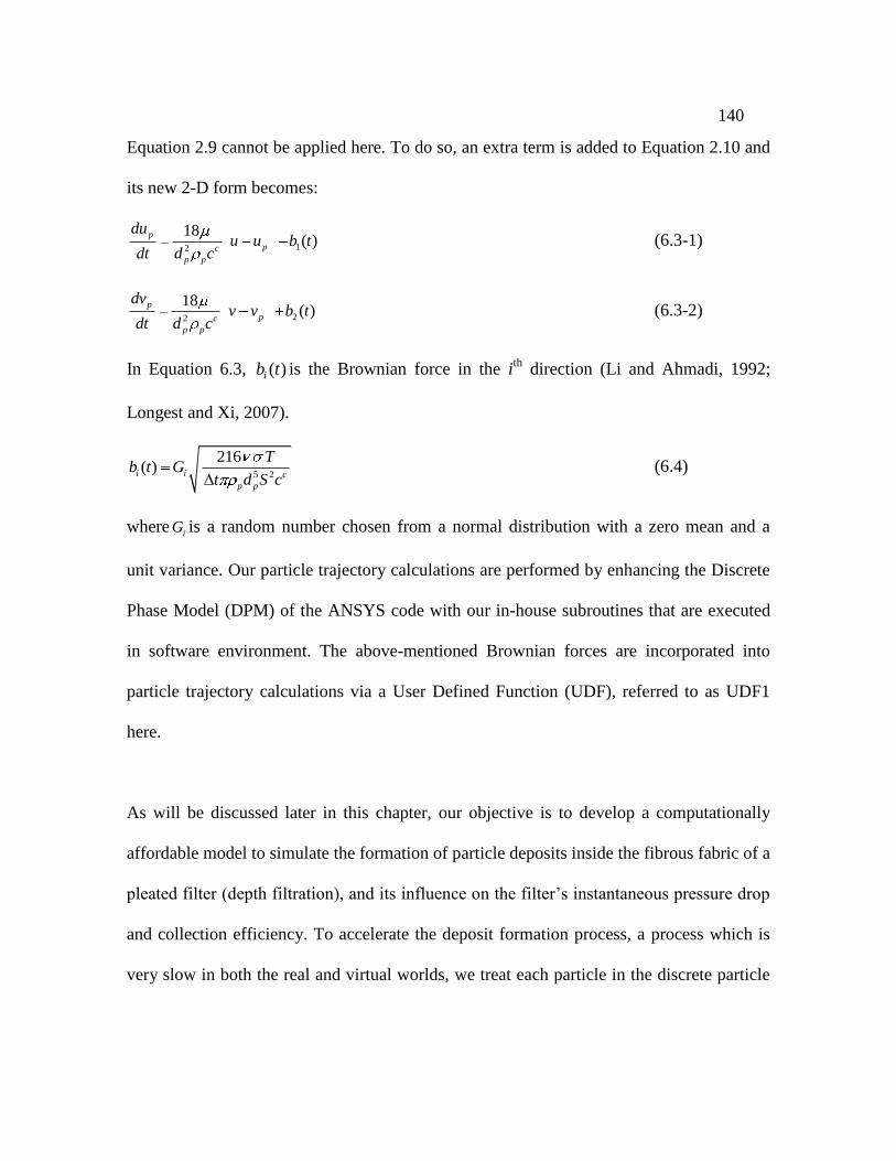
140

Equation 2.9 cannot be applied here. To do so, an extra term is added to Equation 2.10 and

its new 2-D form becomes:

12

18( )

p

pc

p p

duu u b t

dt d c (6.3-1)

22

18( )

p

pc

p p

dvv v b t

dt d c (6.3-2)

In Equation 6.3, ( )ib t is the Brownian force in the ith

direction (Li and Ahmadi, 1992;

Longest and Xi, 2007).

5 2

216( )

Δi i c

p p

Tb t G

t d S c (6.4)

where iG is a random number chosen from a normal distribution with a zero mean and a

unit variance. Our particle trajectory calculations are performed by enhancing the Discrete

Phase Model (DPM) of the ANSYS code with our in-house subroutines that are executed

in software environment. The above-mentioned Brownian forces are incorporated into

particle trajectory calculations via a User Defined Function (UDF), referred to as UDF1

here.

As will be discussed later in this chapter, our objective is to develop a computationally

affordable model to simulate the formation of particle deposits inside the fibrous fabric of a

pleated filter (depth filtration), and its influence on the filter’s instantaneous pressure drop

and collection efficiency. To accelerate the deposit formation process, a process which is

very slow in both the real and virtual worlds, we treat each particle in the discrete particle

141

tracking model as a clusters of particles of the same size. It is then possible to assume that

a cluster continuously deposits fractions of its mass (i.e., particles) as it travels through a

fibrous material. In other words, each computational cell inside the fibrous media acts as a

standalone virtual filter (with fiber diameter and SVF same as the whole fibrous fabric, but

a thickness equal to the size of the cell) that collects a fraction of the cluster’s mass. The

mass of each cluster is considered to be 13, 3 10t jm kg regardless of its diameter. With

this numerical scheme, one does not need to repeat the particle injection process thousands

of times or more to simulate the formation of particle deposit inside a fibrous medium.

6.3 Macro-Scale Modeling of Dust-Loaded Fibrous media

To model the deposition of aerosol particles inside a fibrous medium, the fibrous structure

is treated as a lumped porous layer in which the particles can deposit over time. This

causes the layer’s permeability and particle collection efficiency to change over time. In

contrast to our previous micro-scale modeling work (Chapters2–4), in which the micro-

structure of the fibrous structures were directly included in our simulations, in the current

simulations, the effects of microstructural parameters are fed to a macro-scale model that

simulates the entire dimensions of the filter. To accomplish this, a series of in-house

subroutines are developed to run simultaneously with the flow solver of the ANSYS code

for changing the local properties of the above-mentioned porous layer over time. In this

method, the SVF of each computational cell inside the filter media must be monitored and

increased in response to particle deposition. Ultimately, when the SVF of a cell reaches a

given limit, that cell has to become impermeable to particles (but not to air). The SVF for a

142

cell is defined as the ratio of the volume of deposited particles (and existing fibers) to the

volume of the cell.

In reality, the particle deposit formation inside a filter is a very slow process. Developing a

virtual simulation of this phenomenon requires extensive CPU time. To accelerate particle

deposit formation in our simulations, we have developed a new modeling strategy in which

each aerosol particle entering the domain (the discrete phase) is assumed to be a cluster of

imaginary particles (replicas) with the same size as the cluster itself, as mentioned in the

Section 6.2. The number of imaginary particles in each cluster cln is designed to be an

input depending on the actual size of the particle and the desired CPU time (the initial

mass of a cluster is a constant number arbitrarily chosen to be 13, 3 10t jm kg). Injecting

a cluster containing, for example, 1000 imaginary particles and tracking its trajectory

throughout the filter resembles the situation in which the trajectory of such a particle,

injected at the same location at the inlet, is tracked 1000 times. As our cluster travels

through the fibrous zone, it loses some of its mass in each computational cell to

proportional to the fraction of the above 1000 particles that will be filtered by the media.

Knowing the initial mass of a cluster at the inlet j,tm and the dimensions of the cells inside

the fibrous media, the mass of particles deposited in each cell can be obtained using the

available cell-model (see Tables 1.2–1.4) given in Chapter 1. Here, j is a counter for the

number of clusters in a single injection batch at the inlet. The initial mass for the thj cluster

in the injection batch can be calculated as:

143

13, 3 10t j p pclm n V (6.5)

The deposited mass d ,km after a cluster passes through a computational cell is:

d ,k i , j o, jm m m (6.6)

where the counter k refers to the number of clusters passing through any particular cell

(different from counter j , which is the particle identification number in the injection

batch), and d ,km is the deposited mass after the thk cluster has passed through a particular

cell (see Figure 6.2). The cell’s SVF can be calculated as follows:

,

V

p d k

c

c p

N m (6.7)

The flow field must be recalculated after each batch injection. However, before flow

recalculation, the permeability of the computational cells inside the fibrous domain should

be updated. To do so, we assume that the deposited particles make a permeable granular

medium around the fibers. For simplicity, we assume the fibrous and granular porous

media to act like resistors in series. We therefore update the directional permeability

components of the fibrous zone and obtain effective permeability constants as follows:

1 1 1

1 1 1

lay

IP IP g

lay

TP TP g

k k k

k k k

(6.8)

Where, the permeability of the particle bed ( gk ) is calculated using the Kozeny–Carman

expression (Dullien, 1991):

144

2 3

2180 1

p

g

dk (6.9)

As can be seen in Equation 6.9, permeability of a granular cake strongly depends on its

porosity which can be calculated using the result of Equation 6.7.

The SVF of cells collecting particles will eventually reach a maximum value. This value is

the minimum allowable porosity of a granular bed comprised of a given particle size.

Determining the porosity of the particle bed produced by the deposition of dust particles

inside a filter medium is a challenging task. We used the empirical correlation of Kasper et

al. (2010) obtained for mono-dispersed particles:

0.36 0.44 exp 0.29p

m p

w

d (6.10)

Note that in this equation particle diameter pd is in micrometers. It is worth mentioning

that the macro-scale modeling algorithm developed in this section of the dissertation for

predicting the instantaneous pressure drop and collection efficiency of pleated filters is

computationally quite inexpensive. The simulations presented in this study took on average

about 3–4 hours on a single CPU with a speed of 2.50 GHz. The simulation domains

considered for the study were meshed using 40000 to 250000 triangular cells depending on

the geometry. Mesh-independency has been ensured by monitoring the pressure drop

values obtained for clean media. Simulations presented here are obtained by considering

14 mesh-points across the thickness of the fibrous zone.

145

6.4 Model Implementation and Validation

6.4.1 CFD Implementation

Our simulation procedure starts by first solving the flow field inside the domain. With the

local velocity vectors at each computational cell available, we trace each cluster and if this

cluster is inside the filter domain, estimate the collection efficiency of each cell inside the

fibrous zone by developing a new UDF, hereon referred to as UDF2, using equations given

in Chapter 1. Since the DPM module of the ANSYS considers a particle as a point mass

instead of an object with a finite size, UDF2 also modifies ANSYS’s standard particle

tracking scheme to include particle deposition via interception, which is especially

important for particles depositing on previously deposited particles.

Continued particle injection results in an increase in the mass of the deposited particles

inside the cells. With the mass of deposited particles and their diameter available, new

SVFs (and so new permeability constants) will be assigned to the affected cells via a third

UDF (UDF3) that incorporates Equation 6.7 into the calculations. This procedure will be

repeated until the SVF of a cell inside the medium reaches a certain value obtained using

Equation 6.10. If a blocked cell is located upstream of the fibrous zone, further particle

encounters will result in surface deposition (as opposed to the depth deposition). We stop

our particle loading simulations before surface loading begins, as it is outside the scope of

the current study.

146

We define a User Defined Memory (UDM) for cells that are filled with particle deposits to

mark them as “blocked”. UDMs are allocated memory storage locations which are

assigned to each computational cell in the ANSYS code. When a cluster passes through a

cell within the fibrous domain, the amount of deposited mass must be recorded. To do so,

we defined another UDM for the amount of mass deposited in each cell. With the mass of

particles deposited in each cell recorded, UDF2 updates the SVF of the cells and stores the

information in another UDM. An additional UDF, hereon called as UDF4, is also

developed to update the permeability tensor of the affected cells. The above steps are

shown more systematically in the flowchart shown in Figure 6.3. The final UDF (UDF5)

that we have introduced into our simulation maintains the random injection of particles

into the domain.

6.4.2 Validation

To investigate how accurately the above methodology can simulate reality, we considered

a flat sheet filter––the only case for which some analytical/experimental correlations are

available. We started our investigation by modeling pressure drop and collection efficiency

for a clean filter. As can be seen in Figure 6.4, for a flat sheet with an SVF of 5%, a fiber

diameter of 15 µm, and an inlet air velocity of 0.2 m/s, our model predicts clean filter

collection efficiency values (shown in terms of 0ln ( ) /P t ) in perfect agreement with the

cell-model equations given in Chapter 1. Since the same equations are used in the

calculations shown in Figure 6.4, this agreement only indicates that there are no errors with

regards to the implementation of the cell-model equations in our simulations.

147

To simulate particle-loaded filters, we allow the particles to deposit inside the fibrous

domain. Figure 6.5 shows an example of our particle deposition simulations inside a flat

fibrous sheet at two different times during particle deposition. Particles have a diameter of

10 µm and the air inlet velocity is 0.05 m/s. Formation of particle dendrites and the

preferential paths of minimum resistance chosen by the streamlines can easily be seen in

this figure and its magnified subfigures. Here Black to white shows SVF of the cells in the

fibrous zone. The maximum allowable SVF is 0.6 here.

Only a few empirical correlations are available for predicting the instantaneous pressure

drop of a fibrous medium. Thomas et al. (2001) presented a semi-empirical expression to

obtain the pressure drop of loaded flat-sheet fibrous media,

0Δ Δ inp p κu m (6.11)

where κ is defined as 2 3(1 ) / ( )c

k p ph a c . Note that kh is the Kozeny constant

considered to be 5 for spherical particles. Figure 6.6 shows our pressure drop predictions

as a function of the mass of deposited particles for two different particle diameters and at

two different flow velocities. The predictions of Equation 6.11 are also added to this figure

for comparison. It can be seen that our instantaneous pressure drop calculations match

reasonably well with the predictions of Equation 6.11. Note that the x-axis in this figure is

the deposited mass m , non-dimensionalized using the mass of a single particle. After each

flow batch injection (i.e., time step), the total amount of mass deposited inside the fibrous

zone is recorded and used in Equation 6.11.

148

It is hard to present a one-to-one validation for our instantaneous collection efficiency

calculations here, only because most existing expressions for collection efficiency in the

literature require a variety of case-dependent empirical coefficients. However, to show that

our results for collection efficiency (penetration) follow a reasonable trend, we used the

expression of Kanaoka et al. (1980) as given below.

0 1E E m (6.12)

where λ is an empirical factor obtained here via curve fitting. 0E is the total single fiber

collection efficiency of a clean fiber. Figure 6.7 shows our predictions of 0ln ( / )P P as a

function of the mass of particle deposit in the filter. Equation 6.12 is fitted into our results

to better illustrate the trend of our simulation results.


In this section, we simulate filters with V-shaped pleats. In-plane and through-plane

permeability constants for the filter material are obtained using Equations 1.19 and 1.20 to

be 105.028 10lay

IPk m2 and 103.117 10lay

TPk m2, respectively. We considered filters with 4,

6, 8, 10, and 12 pleats per inch. To study the performance of clean filters, we considered

the particles ranging in size from 100 nm to 10 µm. With the unsteady simulations (filter

aging simulations), however, we only considered particles of 100 nm and 3 µm diameters.

These particles are chosen to simulate performance of our filters against low- and high-

inertia particles.

149

6.5.1 Clean Pleated Filters

Figure 6.8 shows 0ln ( ) /P t for filters with different pleat counts. Our results indicate that,

for light particles (e.g., submicron particles), higher collection efficiencies can be achieved

by increasing the pleat count. However, the effect of pleat count on collection efficiency is

negligible, or even becomes reserved, when particles are inertial (e.g., particles with a

diameter of about 10 microns). Note that as can be seen in Figure 6.8, this trend is valid for

at least any inlet velocities between 0.05 to 0.5 m/s. The effects of pleat count on collection

efficiency can be better explained by reporting the area-averaged face velocity over the

filtration surface in Figure 6.9a. It can be seen that face velocity decreases with increasing

pleat count. This improves particle capture due to Brownian diffusion, but adversely

affects particle capture due to inertial impaction. Therefore, the collection of a filter

changes depending on which capture mechanism is dominant for the given particle size.

Pressure drop values obtained for our clean pleated filters are presented in Figure 6.9b for

inlet velocities of 0.05 and 0.5 m/s. It can be seen that there exists an optimum pleat count

at which pressure drop is minimized, as expected.

6.5.2 Particle-Loaded Pleated Filters

To simulate particle-loaded filters, we allow the particles to deposit inside the fibrous

domain. Figure 6.10 shows an example of our particle deposition simulations inside V-

shaped geometries. Note how the streamlines adjust their paths between the particle

dendrites to flow through the most permeable regions.

150

In Figures 6.11, we present the influence of pleat count on the instantaneous performance

(pressure drop and collection efficiency) of pleated filters versus time for two different

particle diameters of 100 nm and 3 µm and flow velocities of 0.05 and 0.5 m/s. Note in

these figures that simulation time is different for aerosols with different particle diameters

or velocities. This is because, as mentioned before, each particle injection represents a time

interval equal to one second, and to accelerate particle deposit formation process, we have

assumed each injected particle to be a cluster of many particles with the same diameter as

the cluster itself. Therefore, injecting a batch of clusters with each cluster containing

cln particles accelerate the simulation time by a factor of cln . Note again that since loading

is a slower process for smaller particles, we have chosen a larger value for cln when

simulating small particles. The cln values are obtained by considering a constant mass for

the clusters regardless of their size. It is important to note that although a constant mass is

considered for each cluster 13, 3 10t jm kg (and the number concentration of the clusters

at the inlet has been kept at 92 10C m-3

) this does not mean that the mass concentration

of the aerosol particles has been kept constant for all the simulations reported here. The

value considered for the mass of our clusters is only an arbitrary number and does not need

to be held constant when varying the particle diameter. In our simulation method, the

number concentration of the aerosol particles is help constant kept at 92 10C m-3

and the

concept of clusters and imaginary particles within a cluster are only a means of advancing

in time without actually repeating the particle injection process.

151

The results shown in Figures 6.11and 6.12 indicate that the rate of increase of pressure

drop and collection efficiency decreases by increasing the number of pleats. This is chiefly

due to the fact that when a pleated filter is exposed to a given aerosol flow, each pleat

receives less number of particles when increasing the pleat count. Also note that increasing

the flow rate (flow speed) increases the rate of pressure drop increase, as expected (see

Figures 6.11a–d). Similarly, pressure drop increases much faster when particles are larger

(note that all filters are exposed to an aerosol with a fixed number concentration rather than

fixed mass concentration). As can be seen in Figures 6.12a–d, the rate of change of

collection efficiency is more for filters with less number of pleats. The information given

in Figures 6.11–6.12 clearly demonstrate that the new algorithm developed in this work

can be used to predict the instantaneous pressure drop and collection efficiency of a fibrous

filter in its entire actual dimensions and with an affordable computational time.

6.6 Conclusions

This Chapter has been focused on developing a novel macro-scale model for studying the

aging of pleated filters. To date, the current work is the only numerical simulation capable

of quantifying the effects of dust deposition inside the fibrous fabric of pleated filter media

to predict the instantaneous pressure drop and collection efficiency of a filter. Our

simulations with pleated filters exposed to flows of aerosol particles with different

diameters and velocities indicate that increasing the number of pleats decelerates the aging

of a filter. It was also shown that increasing the speed of the flow or the diameter of the

aerosol particles accelerates the aging process, if the aerosol number concentration is held

152

constant. Our algorithm has been used to obtain pressure drop values for dust loaded flat

sheet media. These values are compared with the experimental data reported by Thomas et

al., (2001), and good agreement has been observed.

153

2θ

inle

tSymmetry

Symmetry

outlet

W

Figure 6.1: Simulation domain for triangular pleats with a pleat angle of 2θ and a pleat

height of L .

md,1

md,2

md,3

…

md,kmi,j mo,j

mass deposited by

the 1st cluster that

entered the cell

mass deposited by

the kth cluster that

entered the cell

jth cluster

among those

injected at

the inlet

Figure 6.2: Schematic illustration of transient particle deposit increase inside a

computational cell.

154

Yes

start

Inject a cluster

Cluster inside

filter medium

No

Cluster touches

any blocked

cell

Yes Cluster deposits

No

Cell is

empty

Calculate cell path length and

obtain flow speed inside the cell

Find EΣ for the cell

Record the amount of mass

inside the cell

Mark the cell as not empty

Cluster leaves the cell

with reduced mass

Yes No

Find EΣ for the cell

Add the deposited mass to the

current mass and record it

Specify the SVF and

permeability to the cell

αc > αu

Cell will be blocked

Yes

No

Cluster

reaches

downstream

No

Yes

All

clusters

are

processed

No

Recalculate

flow

Yes

All

Clusters

are

processed

Recalculate

flow

Yes

No

Assign a new batch

UDF5

UDF1

UDF1 UDF2

UDF2

UDF1

UDF2

UDF3

UDF3

UDF2

UDF2

UDF4

UDF2

UDF3

UDF1

UDF4UDF4

UDF2

UDF3

UDF3

UDF3

UDF3

UDF1

UDF2

UDF2

UDF2

Figure 6.3: Numerical simulation flow chart. At each stage, the effective UDF has been

mentioned.

155

dp

(µm)

-ln

(P)/

t(1

/m)

10-1

100

101

101

102

103

Simulation

Semi-empirical

df= 15 (µm)

= 0.05

Figure 6.4: Comparison between our simulation outputs and the cell model semi-empirical

equations for particle penetration through a clean fibrous medium. The cell model

equations are shown in Chapter 1.

156

(a) (b)

Figure 6.5: Contour plots of cell SVF together with air streamlines showing an example of

particle deposition inside the fibrous zone at two different simulation times of 40t s (a),

and 180t s (b). The simulations are conducted with a particle diameter of 10pd µm at

a speed of 0 05inu . m/s. The fibrous medium is assumed to have a SVF of 5% and a fiber

diameter of 15fd µm with the thickness of 0.7mm. Maximum allowable SVF is obtained

accordingly from Equation 6.10.

157

m*

p(P

a)

0 1000 2000

2

2.1

2.2

CFD implementation

Semi-empirical

dp= 10 µm

uin= 0.05 m/s

m*

p(P

a)

0 200 400 600 800

0

20

40

60CFD implementation

Semi-empirical

dp= 10 µm

uin= 0.5 m/s

m*

p(P

a)

0 5E+07 1E+08

0

20

40

60CFD implementation

Semi-empirical

dp= 100 nm

uin= 0.05 m/s

m*

p(P

a)

0 5E+06 1E+07 1.5E+07

20

22

24

CFD implementation

Semi-empirical

dp= 100 nm

uin= 0.5 m/s

,Thomas (2001) ,Thomas (2001)

(a) (b)

(d)(c)

,Thomas (2001) ,Thomas (2001)

Figure 6.6: Comparison between our pressure drop predictions and those of the semi-

empirical expression of Thomas et al. (2001) for fibrous flat sheets during dust deposition.

The fibrous medium is assumed to have a SVF of 5%, a fiber diameter of 15fd µm, and

a thickness of 0.7mm.

158

(a) (b)

(d)(c)

m*

-ln

(P/P

0)

0 1000 2000

0

0.005

0.01

0.015

CFD implementation

Semi-empirical

dp= 1 µm

uin= 0.5 m/s

m*

-ln

(P/P

0)

0 200 400 600 800

0

0.02

0.04

0.06CFD implementation

Semi-empirical

dp= 1 µm

uin= 0.5 m/s

m*

-ln

(P/P

0)(

10

-2)

0 1E+07

0

0.02

0.04

0.06

0.08

CFD implementation

Semi-empirical

dp= 100 nm

uin= 0.5 m/s

m*

-ln

(P/P

0)

0 5E+07 1E+08

0

0.02

0.04

0.06CFD implementation

Semi-empirical

dp= 100 nm

uin= 0.05 m/s

, Kanaoka (1980) , Kanaoka (1980)

, Kanaoka (1980) , Kanaoka (1980)

Figure 6.7: Our collection efficiency predictions are used along with the semi-empirical

expression of Kanaoka et al. (1980) for particle penetration through fibrous flat sheets

during dust deposition. The curve fitting parameters are (a) λ=5000, (b) λ=3000, (c) λ=250,

and (d) λ=500. The fibrous medium is assumed to have a SVF of 5%, a fiber diameter of

15fd µm, and a thickness of 0.7mm.

159

X

X

X

X

X

X

X

dp

(µm)

-ln

(P0)/

t(1

/m)

10-1

100

101

500

10004 Pleat/in

6 Pleat/in

8 Pleat/in

10 Pleat/in

12 Pleat/in

X

V-shaped

uin

= 0.05 (m/s)

X

X

X

X

X

X

X

dp

(µm)

-ln

(P0)/

t(1

/m)

10-1

100

101

500

10002 Pleat/in

3 Pleat/in

4 Pleat/in

5 Pleat/in

6 Pleat/in

X

V-shaped

uin

= 0.5 (m/s)

(a)

(b)

X

X

X

X

X

X

X

dp

(µm)

-ln

(P0)/

t(1

/m)

10-1

100

101

500

10004 Pleat/in

6 Pleat/in

8 Pleat/in

10 Pleat/in

12 Pleat/in

X

V-shaped

uin

= 0.5 (m/s) (b)

Figure 6.8: Particle penetration per thickness obtained for clean filters with different pleat

counts at two different air inlet velocities of 0.05 and 0.5 m/s.

Pleat count (1/in)

ufa

ce(m

/s)

4 6 8 10 12

0.05

0.1u

in= 0.5 (m/s)

uin

= 0.05 (m/s)

V-shaped

(a)

Pleat count (1/in)

p0

(Pa)

4 6 8 10 1210

-1

100

101

uin

= 0.5 (m/s)

uin

= 0.05 (m/s)

kTP

lay= 3.117 x 10

-10& k

IP

lay= 5.028 x 10

-10

V-shaped(b)

Pleat count (1/in)

ufa

ce(m

/s)

4 6 8 10 12

0.05

0.1u

in= 0.5 (m/s)

uin

= 0.05 (m/s)

V-shaped

(a)

Pleat count (1/in)

p0

(Pa)

4 6 8 10 1210

-1

100

101

uin

= 0.5 (m/s)

uin

= 0.05 (m/s)

kTP

lay= 3.117 x 10

-10& k

IP

lay= 5.028 x 10

-10

V-shaped(b)

Figure 6.9: Effects of pleat count of the face velocity (a) and pressure drop (b) obtained for

clean filters at two different air inlet velocities of 0.05 and 0.5 m/s. Fibrous media have a

SVF of 5%, a fiber diameter of 15fd µm, a thickness of 0.7 mm.

160


of particle deposition inside the fibrous zone in a pleated filter. The particle diameter and

air inlet velocity are considered to be 3pd µm and 0 05inu . m/s, respectively. Here

SVF is 5%, fiber diameter is 15fd µm, and thickness of 0.7 mm.

161

- - - - - - - - - - - - - - - - - - - - - - - - - -------

-

-

-

-

-

-

-

-

t (s)

ln(P

)/ln

(P0)

0 2000 4000 6000

1

1.5

2

2.54 Pleats/in

6 Pleats/in

8 Pleats/in

10 Pleats/in

12 Pleats/in

-

V-shapedd

p= 3 (µm)

uin

= 0.5 (m/s)

-----------------------------

----------

------

------

--------------

-------

-----------------------------

t (s)

ln(P

)/ln

(P0)

0 5000 10000

1

1.2

1.4

4 Pleats/in

6 Pleats/in

8 Pleats/in

10 Pleats/in

12 Pleats/in

-

V-shapedd

p= 3 (µm)

uin

= 0.05 (m/s)

- - - - - - - - - - - - - - - - - - -- -

------

--

-

-

-

-

-

-

-

-

-

-

-

t (s)

ln(P

)/ln

(P0)

0 5E+07 1E+08

2

4

6 4 Pleats/in

6 Pleats/in

8 Pleats/in

10 Pleats/in

12 Pleats/in

-

V-shapedd

p= 100 (nm)

uin

= 0.5 (m/s)

- - - - - - - - - - - - - - - - - - - - - - - - - - - - -------------

-

--

-

-

-

-

-

-

-

t (s)

ln(P

)/ln

(P0)

0 5E+07 1E+08

1

1.2

1.4

1.6

1.84 Pleats/in

6 Pleats/in

8 Pleats/in

10 Pleats/in

12 Pleats/in

-

V-shapedd

p= 100 (nm)

uin

= 0.05 (m/s)

(e)

(f)

(g)

(h)

- - - - - - - - - - - - - - - - - - - - - --------

-

-

-

-

-

-

-

----

t (s)

p/

p0

0 2000 4000 6000

1

2

3

44 Pleats/in

6 Pleats/in

8 Pleats/in

10 Pleats/in

12 Pleats/in

-

V-shapedd

p= 3 (µm)

uin

= 0.5 (m/s)

-------------------------------------------

------------

-------

------

---------------------------------

t (s)

p/

p0

0 5000 10000

1

1.5

24 Pleats/in

6 Pleats/in

8 Pleats/in

10 Pleats/in

12 Pleats/in

-

V-shapedd

p= 3 (µm)

uin

= 0.05 (m/s)

- - - - - - - - - - - - - - - - --------

-

-

-

-

-

-

----------

t (s)

p/

p0

0 5E+07 1E+08

1

2

3

4

54 Pleats/in

6 Pleats/in

8 Pleats/in

10 Pleats/in

12 Pleats/in

-

V-shapedd

p= 100 (nm)

uin

= 0.5 (m/s)

- - - - - - - - - - - - - - - - - - - - - - - - - - ---------

--

-

--

---

--------

t (s)

p/

p0

0 5E+07 1E+08

2

4

6

8

4 Pleats/in

6 Pleats/in

8 Pleats/in

10 Pleats/in

12 Pleats/in

-

V-shapedd

p= 100 (nm)

uin

= 0.05 (m/s)

(a)

(b)

(c)

(d)

- - - - - - - - - - - - - - - - - - - - - - - - - -------

-

-

-

-

-

-

-

-

t (s)

ln(P

)/ln

(P0)

0 2000 4000 6000

1

1.5

2

2.54 Pleats/in

6 Pleats/in

8 Pleats/in

10 Pleats/in

12 Pleats/in

-

V-shapedd

p= 3 (µm)

uin

= 0.5 (m/s)

-----------------------------

----------

------

------

--------------

-------

-----------------------------

t (s)

ln(P

)/ln

(P0)

0 5000 10000

1

1.2

1.4

4 Pleats/in

6 Pleats/in

8 Pleats/in

10 Pleats/in

12 Pleats/in

-

V-shapedd

p= 3 (µm)

uin

= 0.05 (m/s)

- - - - - - - - - - - - - - - - - - -- -

------

--

-

-

-

-

-

-

-

-

-

-

-

t (s)

ln(P

)/ln

(P0)

0 5E+07 1E+08

2

4

6 4 Pleats/in

6 Pleats/in

8 Pleats/in

10 Pleats/in

12 Pleats/in

-

V-shapedd

p= 100 (nm)

uin

= 0.5 (m/s)

- - - - - - - - - - - - - - - - - - - - - - - - - - - - -------------

-

--

-

-

-

-

-

-

-

t (s)

ln(P

)/ln

(P0)

0 5E+07 1E+08

1

1.2

1.4

1.6

1.84 Pleats/in

6 Pleats/in

8 Pleats/in

10 Pleats/in

12 Pleats/in

-

V-shapedd

p= 100 (nm)

uin

= 0.05 (m/s)

(e)

(f)

(g)

(h)

- - - - - - - - - - - - - - - - - - - - - --------

-

-

-

-

-

-

-

----

t (s)

p/

p0

0 2000 4000 6000

1

2

3

44 Pleats/in

6 Pleats/in

8 Pleats/in

10 Pleats/in

12 Pleats/in

-

V-shapedd

p= 3 (µm)

uin

= 0.5 (m/s)

-------------------------------------------

------------

-------

------

---------------------------------

t (s)

p/

p0

0 5000 10000

1

1.5

24 Pleats/in

6 Pleats/in

8 Pleats/in

10 Pleats/in

12 Pleats/in

-

V-shapedd

p= 3 (µm)

uin

= 0.05 (m/s)

- - - - - - - - - - - - - - - - --------

-

-

-

-

-

-

----------

t (s)

p/

p0

0 5E+07 1E+08

1

2

3

4

54 Pleats/in

6 Pleats/in

8 Pleats/in

10 Pleats/in

12 Pleats/in

-

V-shapedd

p= 100 (nm)

uin

= 0.5 (m/s)

- - - - - - - - - - - - - - - - - - - - - - - - - - ---------

--

-

--

---

--------

t (s)

p/

p0

0 5E+07 1E+08

2

4

6

8

4 Pleats/in

6 Pleats/in

8 Pleats/in

10 Pleats/in

12 Pleats/in

-

V-shapedd

p= 100 (nm)

uin

= 0.05 (m/s)

(a)

(b)

(c)

(d)

Figure 6.11: Instantaneous pressure drop versus time for two different particle diameters of

100 nm and 3µm, and at two different air inlet velocities of 0.05 and 0.5m/s.

162

- - - - - - - - - - - - - - - - - - - - - - - - - -------

-

-

-

-

-

-

-

-

t (s)

ln(P

)/ln

(P0)

0 2000 4000 6000

1

1.5

2

2.54 Pleats/in

6 Pleats/in

8 Pleats/in

10 Pleats/in

12 Pleats/in

-

V-shapedd

p= 3 (µm)

uin

= 0.5 (m/s)

-----------------------------

----------

------

------

--------------

-------

-----------------------------

t (s)

ln(P

)/ln

(P0)

0 5000 10000

1

1.2

1.4

4 Pleats/in

6 Pleats/in

8 Pleats/in

10 Pleats/in

12 Pleats/in

-

V-shapedd

p= 3 (µm)

uin

= 0.05 (m/s)

- - - - - - - - - - - - - - - - - - -- -

------

--

-

-

-

-

-

-

-

-

-

-

-

t (s)

ln(P

)/ln

(P0)

0 5E+07 1E+08

2

4

6 4 Pleats/in

6 Pleats/in

8 Pleats/in

10 Pleats/in

12 Pleats/in

-

V-shapedd

p= 100 (nm)

uin

= 0.5 (m/s)

- - - - - - - - - - - - - - - - - - - - - - - - - - - - -------------

-

--

-

-

-

-

-

-

-

t (s)

ln(P

)/ln

(P0)

0 5E+07 1E+08

1

1.2

1.4

1.6

1.84 Pleats/in

6 Pleats/in

8 Pleats/in

10 Pleats/in

12 Pleats/in

-

V-shapedd

p= 100 (nm)

uin

= 0.05 (m/s)

(e)

(f)

(g)

(h)

- - - - - - - - - - - - - - - - - - - - - --------

-

-

-

-

-

-

-

----

t (s)

p/

p0

0 2000 4000 6000

1

2

3

44 Pleats/in

6 Pleats/in

8 Pleats/in

10 Pleats/in

12 Pleats/in

-

V-shapedd

p= 3 (µm)

uin

= 0.5 (m/s)

-------------------------------------------

------------

-------

------

---------------------------------

t (s)

p/

p0

0 5000 10000

1

1.5

24 Pleats/in

6 Pleats/in

8 Pleats/in

10 Pleats/in

12 Pleats/in

-

V-shapedd

p= 3 (µm)

uin

= 0.05 (m/s)

- - - - - - - - - - - - - - - - --------

-

-

-

-

-

-

----------

t (s)

p/

p0

0 5E+07 1E+08

1

2

3

4

54 Pleats/in

6 Pleats/in

8 Pleats/in

10 Pleats/in

12 Pleats/in

-

V-shapedd

p= 100 (nm)

uin

= 0.5 (m/s)

- - - - - - - - - - - - - - - - - - - - - - - - - - ---------

--

-

--

---

--------

t (s)

p/

p0

0 5E+07 1E+08

2

4

6

8

4 Pleats/in

6 Pleats/in

8 Pleats/in

10 Pleats/in

12 Pleats/in

-

V-shapedd

p= 100 (nm)

uin

= 0.05 (m/s)

(a)

(b)

(c)

(d)

- - - - - - - - - - - - - - - - - - - - - - - - - -------

-

-

-

-

-

-

-

-

t (s)

ln(P

)/ln

(P0)

0 2000 4000 6000

1

1.5

2

2.54 Pleats/in

6 Pleats/in

8 Pleats/in

10 Pleats/in

12 Pleats/in

-

V-shapedd

p= 3 (µm)

uin

= 0.5 (m/s)

-----------------------------

----------

------

------

--------------

-------

-----------------------------

t (s)

ln(P

)/ln

(P0)

0 5000 10000

1

1.2

1.4

4 Pleats/in

6 Pleats/in

8 Pleats/in

10 Pleats/in

12 Pleats/in

-

V-shapedd

p= 3 (µm)

uin

= 0.05 (m/s)

- - - - - - - - - - - - - - - - - - -- -

------

--

-

-

-

-

-

-

-

-

-

-

-

t (s)

ln(P

)/ln

(P0)

0 5E+07 1E+08

2

4

6 4 Pleats/in

6 Pleats/in

8 Pleats/in

10 Pleats/in

12 Pleats/in

-

V-shapedd

p= 100 (nm)

uin

= 0.5 (m/s)

- - - - - - - - - - - - - - - - - - - - - - - - - - - - -------------

-

--

-

-

-

-

-

-

-

t (s)

ln(P

)/ln

(P0)

0 5E+07 1E+08

1

1.2

1.4

1.6

1.84 Pleats/in

6 Pleats/in

8 Pleats/in

10 Pleats/in

12 Pleats/in

-

V-shapedd

p= 100 (nm)

uin

= 0.05 (m/s)

(e)

(f)

(g)

(h)

- - - - - - - - - - - - - - - - - - - - - --------

-

-

-

-

-

-

-

----

t (s)

p/

p0

0 2000 4000 6000

1

2

3

44 Pleats/in

6 Pleats/in

8 Pleats/in

10 Pleats/in

12 Pleats/in

-

V-shapedd

p= 3 (µm)

uin

= 0.5 (m/s)

-------------------------------------------

------------

-------

------

---------------------------------

t (s)

p/

p0

0 5000 10000

1

1.5

24 Pleats/in

6 Pleats/in

8 Pleats/in

10 Pleats/in

12 Pleats/in

-

V-shapedd

p= 3 (µm)

uin

= 0.05 (m/s)

- - - - - - - - - - - - - - - - --------

-

-

-

-

-

-

----------

t (s)p

/p

0

0 5E+07 1E+08

1

2

3

4

54 Pleats/in

6 Pleats/in

8 Pleats/in

10 Pleats/in

12 Pleats/in

-

V-shapedd

p= 100 (nm)

uin

= 0.5 (m/s)

- - - - - - - - - - - - - - - - - - - - - - - - - - ---------

--

-

--

---

--------

t (s)

p/

p0

0 5E+07 1E+08

2

4

6

8

4 Pleats/in

6 Pleats/in

8 Pleats/in

10 Pleats/in

12 Pleats/in

-

V-shapedd

p= 100 (nm)

uin

= 0.05 (m/s)

(a)

(b)

(c)

(d)

- - - - - - - - - - - - - - - - - - - - - - - - - -------

-

-

-

-

-

-

-

-

t (s)

ln(P

)/ln

(P0)

0 2000 4000 6000

1

1.5

2

2.54 Pleats/in

6 Pleats/in

8 Pleats/in

10 Pleats/in

12 Pleats/in

-

V-shapedd

p= 3 (µm)

uin

= 0.5 (m/s)

-----------------------------

----------

------

------

--------------

-------

-----------------------------

t (s)

ln(P

)/ln

(P0)

0 5000 10000

1

1.2

1.4

4 Pleats/in

6 Pleats/in

8 Pleats/in

10 Pleats/in

12 Pleats/in

-

V-shapedd

p= 3 (µm)

uin

= 0.05 (m/s)

- - - - - - - - - - - - - - - - - - -- -

------

--

-

-

-

-

-

-

-

-

-

-

-

t (s)

ln(P

)/ln

(P0)

0 5E+07 1E+08

2

4

6 4 Pleats/in

6 Pleats/in

8 Pleats/in

10 Pleats/in

12 Pleats/in

-

V-shapedd

p= 100 (nm)

uin

= 0.5 (m/s)

- - - - - - - - - - - - - - - - - - - - - - - - - - - - -------------

-

--

-

-

-

-

-

-

-

t (s)

ln(P

)/ln

(P0)

0 5E+07 1E+08

1

1.2

1.4

1.6

1.84 Pleats/in

6 Pleats/in

8 Pleats/in

10 Pleats/in

12 Pleats/in

-

V-shapedd

p= 100 (nm)

uin

= 0.05 (m/s)

(e)

(f)

(g)

(h)

- - - - - - - - - - - - - - - - - - - - - --------

-

-

-

-

-

-

-

----

t (s)

p/

p0

0 2000 4000 6000

1

2

3

44 Pleats/in

6 Pleats/in

8 Pleats/in

10 Pleats/in

12 Pleats/in

-

V-shapedd

p= 3 (µm)

uin

= 0.5 (m/s)

-------------------------------------------

------------

-------

------

---------------------------------

t (s)

p/

p0

0 5000 10000

1

1.5

24 Pleats/in

6 Pleats/in

8 Pleats/in

10 Pleats/in

12 Pleats/in

-

V-shapedd

p= 3 (µm)

uin

= 0.05 (m/s)

- - - - - - - - - - - - - - - - --------

-

-

-

-

-

-

----------

t (s)p

/p

0

0 5E+07 1E+08

1

2

3

4

54 Pleats/in

6 Pleats/in

8 Pleats/in

10 Pleats/in

12 Pleats/in

-

V-shapedd

p= 100 (nm)

uin

= 0.5 (m/s)

- - - - - - - - - - - - - - - - - - - - - - - - - - ---------

--

-

--

---

--------

t (s)

p/

p0

0 5E+07 1E+08

2

4

6

8

4 Pleats/in

6 Pleats/in

8 Pleats/in

10 Pleats/in

12 Pleats/in

-

V-shapedd

p= 100 (nm)

uin

= 0.05 (m/s)

(a)

(b)

(c)

(d)

((a)

(b)

(c)

(d)

(a)

(b)

(c)

(d)

Figure 6.12: Instantaneous penetration versus time for two different particle diameters of

100 nm and 3µm, and at two different air inlet velocities of 0.05 and 0.5m/s.

163

CHAPTER 7 Macro-Scale Modeling of Pleated Filters

Challenged with Poly-Disperse Aerosols

7.1 Introduction

Pleated filters are used in vast areas of application in automotive industry, HVAC systems,

and clean rooms among many others, especially when high performance in aerosol

filtration or compact design of filters is required. Controlling the air flow inside pleats is an

essential consideration which leads to minimizing pressure drop and maximizing particle

collection efficiency. as mentioned in previous two chapters, air flow control in pleated

filters usually depends on two major contributors. As discussed earlier, one is the fibrous

medium or flat sheet thin paper, which will be folded to make pleats. The second is the

pleat geometry (i.e. pleat width, pleat height and pleat shape) which can influence the

performance of the filter due to viscous effects. In addition, there is another factor involved

which can affect filter performance and that is dust deposition. In general, most of the

published research in studying pleated filters is concentrated on optimizing pleats to

minimize pressure drop (the related works have been cited in Chapter 5). To date, there are

no criteria for designing pleat shape and pleat count for optimizing both the pressure drop

and collection efficiency. More importantly, the influence of particle loading (i.e., filter

aging) on performance of fibrous filters has never been studied in the past. There only two

Content of this section is currently in the final stages of preparation for submission to an engineering

journal for publication.

164

studies can be found: analytical work of Rebai et al., (2010), our own works (Fotovati et

al., 2011; this work was previously presented in Chapter 5). In our work the effects of

micron-sized dust deposition on pressure drop of HEPA filters were simulated. In addition,

we introduced a numerical scheme which allows obtaining the deposition pattern of the

particles inside the fibrous filters (Fotovati et al., 2011, this work was previously presented

in Chapter 6) and also studying the collection efficiency of pleated filters.

The first two aforesaid works are limited to some sort of simplifications and mainly

covered surface deposition and monitored pleats pressure drop, while the latter is just

proposing a methodology to model in-depth dust deposition and measure the collection

efficiency of pleated filters. This part of the study, however, provides the most realistic and

comprehensive study about the performance of pleated filters to date. In this chapter, we

combine the depth and surface deposition and it is of the interest to investigate whether our

achievements for surface-only deposition can be verified when depth deposition is

included. We also allow the aerosol particles to be poly-dispersed in size and model their

deposition pattern. We consider the fibrous structure as a lumped porous zone, and

particles will be filtered inside the zone due to cell model equations for a fibrous domain.

When there is a poly-dispersed surface dust cake however, we assume that the cake acts as

a granular bed of spherical collectors (deposited particles in this case) and we therefore

solve the related equations at the outside cake for particle filtration. In addition, we assume

aerosol with range of particle-size distribution, and also, if it is acceptable, particles are

allowed to penetrate into currently deposited dust cakes. This novel methodology provides

165

the most complete and general study about the performance of pleated filters under dust-

load effects.

The flow field is modeled exactly the same fashion as we discussed in previous two

chapters. To track the aerosol particles and determine their paths through the filter, we

consider the same Lagrangian approach, introduced in previous chapter. Our particle

trajectory modeling and flow calculations are performed by enhancing the Discrete Phase

Model (DPM) of the ANSYS CFD code with our in-house subroutines (UDF’s) that are

executed in ANSYS’s environment. The strategy for particle tracking (both for depth and

surface deposition) is based on assigning a mass to each injected particle and monitoring

the rate of deposition. This means that we considered each injected particle as a group of

same size sub-particles (see Chapter 6 for more details).

7.2 Modeling of Dust Deposition

Instead of modeling Dust deposition inside the fibrous micro-structure, it is modeled while

fibrous media are considered as lumped porous region (for simulation domain see Figure

6.1 from previous chapter). Therefore, the particles can deposit over time, and their

permeability and collection efficiency would change as deposition occurs. In our

simulations we calculate the amount of mass deposition inside each computational cell

after each individual dust clusters pass across it, and the values for permeability would be

updated for flow recalculation. In addition, when dust clusters leave the filter, the amount

of mass which they carry is known and after all particles clusters are injected, the filter

166

penetration can be predicted inside simulation domain. The SVF for each cell is estimated

by knowing the amount of deposited mass in that cell and its volume. The maximum

allowable SVF (maxα ) for each cell is found according to the deposited particle diameter in

that cell using Equation 6.10 (Kasper et al., 2010). If the cell SVF is greater than the

predicted value by equation 6.10, then this cell is impermeable to the incoming particles

with diameter of pd . The flow field must be recalculated after each batch injection.

However, before flow recalculation, the permeability of the computational cells inside the

fibrous domain should be updated. To do so, we assume that the deposited particles make a

permeable granular medium around the fibers. For simplicity, we assume the fibrous and

granular porous media to act like resistors in series (see Equations 6.8 and 6.9).

With mono-dispersed particles, all injected particles have identical diameter ( pd ) and

therefore, no further consideration regarding particle diameter is necessary. The particle

tracking follows perfectly the steps presented in Figure 6.3 in previous chapter. First,

particle clusters enter the fibrous domain, and the cell model equations for cylindrical

fibrous structures are solved inside each computational cell using cell model equations

introduced in Chapter 1. According to these calculations, the permeability change due to

granular particle deposition inside the fibrous domain will be calculated and the directional

permeability components related to the fibrous domain will be updated before flow

recalculation. When a cell’s SVF reaches to its maximum allowable value, then if any

cluster touches this cell, all of its mass will deposit at once. This process will be taken

167

place until the cells adjacent to the filter surface are blocked. At this point, surface

deposition starts.

With surface deposition starts, then any newly incoming particle is faced with the granular

beds of previously deposited particles (granular filter). At this stage, we solve the cell

model equations for granular collectors (equations A1–A5 in Appendix A) inside cells that

contain deposited mass with the diameter of pd . The cells’ SVF will be assigned based on

the deposited mass and whenever the SVF is greater than the maximum allowable value,

the cell will be blocked and is not allowed to admit anymore particles.

7.3 Poly-Dispersed Particle Consideration

The main objective of this chapter is to study the influence of poly-dispersed dust

deposition on the performance of pleated geometries. It is important to note that with

polydisperse aerosol injection, particles may penetrate through already deposited cakes. To

conduct this study, we need to assign an equivalent diameter for each cell, when different

clusters with different diameters deposit inside it. A general definition for an average

particle diameter is given as (Dullien, 1992):

0

0

rp p p p

rp p p

d d n d d d

d

d n d d d

(7.1)

where pn d is the density function (number fraction) of each particle diameter. The

value 0r gives the result for the number average diameter. For the value of 2r , the

168

above expression gives the surface average, and with 3r , it gives the volume average

diameter. According to the works of Macdonald et al. (1979) and Rumpf and Gupte

(1971), the best results are obtained by the surface averaging method (i.e. 2r ). Thus in

the current work, we use this method to predict the average particle diameter inside each

cell.

We assumed that inside each cell, we deal with two different particle sizes, an averaged

diameter of already deposited particles in the cell ( pd ) and the diameter of currently

incoming cluster ( pd ). Therefore Equation 7.1 can be simplified to the following format:

3 3

2 2

p pp p

p pp p

d dd d

p

d dd d

n d n dd

n d n d (7.2)

In above,pd

n and pdn are the number fractions (density functions) for already deposited

particles and incoming particle, respectively. To find these number fractions, we simply

use the following:

p

p p

pp p

p

pp

pp p

dd

d ddd d

cl dd d

d d d

NmN n

m N N

m NN n

m N N

(7.3)

Parameter N refers to the exact number of particles while n is their fractional value

( 0 1n ). Also note that dm and clm are the cell’s deposited mass and incoming cluster

mass, while pd

m is the mass of one single particle with the diameter identical to that of the

169

averaged deposited particle in each cell, and pdm is the mass of single particle inside the

incoming cluster. Figure 7.1 shows these steps in a flow chart format. To add above

considerations into our simulations, we modified our UDF for particle-tracking, in such a

way that it checks for previously deposited mass inside each computational cell and

assigns the average dust particle diameter to it, where this diameter will be considered as

collector diameter in Equations A1–A4. Knowing incoming clusters’ diameters, and their

mass fractions, poly-dispersed dust deposition in pleated geometry can be modeled.


In the current work, we consider triangular (V-shaped) pleats with different widths (or

angles) but an identical length of 25.4 mm (same as what we have shown in Figure 6.1).

The pleat width is set in a sort of way that we model filters with 4, 8, and 12 pleats per

inch. The fibrous medium is assumed to have a thickness of 0.7 mm, SVF of 7.5%, and

fiber diameter of 15µm. Two different inlet air velocities of 0.05 m/s and 0.5 m/s with a

constant aerosol number concentration of 92 10C m-3

are considered in this study. Note

that the inlet velocity is the velocity of the air flow at the inlet to the filter package (or the

duct in which the filter is mounted) and should not be confused with the face velocity,

which is the air velocity as it enters the fibrous medium. Since our simulation domain is

two-dimensional, we assume a unit length for the dimension perpendicular to the

simulation plane (x-y plane). An equivalent particle concentration is obtained based on the

concentration flux at each time. Note that each injection batch resembles a time interval

170

equal to one second. After each injection we recalculate the flow field and monitor and

report the pressure drop and penetration changes. We injected particles with 1 and 10

micron in size as a sample for our mono-dispersed particle injection. To model poly-

dispersed particle deposition, we used particles with size dispersion between 1µm and 10

µm follows a lognormal distribution with mean diameter of 4.53 µm and standard

deviation of 0.733.

7.4.1 Mono-Dispersed Dust Loaded Filter Performance

At first our results for the effects of particles size and inlet velocity (inertia) on the

performance of pleated filters are presented. . Figure 7.2a–b gives the dust pattern inside

filters with 4, 8 and 12 pleats per inch for low and high inertial particles, respectively. In

Figure 7.2a, low inertial particles with 1µm diameter and 0.05 m.s-1

injection speed, shows

a very uniform deposition, no significant dendrite has been observed and in addition, the

depth deposition is not negligible as can be seen. Accordingly, no filter blocking can be

detected. With high inertial particles injection (Figure 7.2b), the depth deposition is not

dominant and surface deposition has been occurred faster compare to low inertial particle

injection. As was expected, large dendrites have been formed and blocked the filter. Note

that due to the random nature of dust injection, these dendrites may occur at any location

over the pleat surface or at any time. These blocking inside the pleat channels can be

detected faster when dealing with more number of pleats. Note that in this study, we did

not take particles bouncing into account.

171

In Figures 7.3 and 7.4, we reported transient pressure drop and collection efficiency

increase ratio during time. Each of our time steps represents one second, however, due to

simulations artifact (i.e. filter geometry generation simplifications) we decided to report

simulation times with an arbitrary unit. Figure 7.3a–b shows that filters with more number

of pleats always has less pressure drop and collection efficiency increase ratio, when they

are dealing with low inertial particles. Even though we let the simulations to continue for

long simulating time, no blocking by dendrites has been observed. With higher inertial

particles injection, as can be seen in Figure 7.3c–d, no significant change occurred

compare to results of Figure 7.3a–b. The values for maximum pressure drop and collection

efficiency increase ratio are significantly higher compare to very low inertial particles, and

the reason is due to higher aerosol flux that is injected into filter at each time step. Filters

with more number of pleats have higher pressure drop and collection efficiency increase

ratio and our results are in complete agreement with our previous work (Fotovati et al.,

2011). This trend cannot be observed as filter encounters with very highly inertial particles.

As Figure 7.4a–b depicts, even after a very short while, the filter is getting blocked by

dendrites and because this phenomenon happens faster for filters with higher number of

pleats, therefore, they have higher pressure drop and collection efficiency ratio.

7.4.2 Poly-Dispersed Dust Loaded Filter Performance

The graphical demonstrations of particle deposition pattern have presented in Figure 7.5a–

b. We let the simulations to run for 152000 time steps and as can be seen, regardless of

172

particle inertia, all of our simulations resulted in filter blocking by dust cake. In addition as

can be seen in Figure 7.5, depth filtration is important as well. The reason can be defined

regarding to the particles distribution. As is known, due to log-normal distribution, in each

injection batch there are a greater number of fine particles than large size particles, and as

we discussed in previous section, with smaller particle size, depth filtration must be

considered.

Figure 7.6a–b shows the increase ratio for filter pressure drop and collection efficiency for

filter faces with low inertial particles injection. As can be seen, unlike pressure drop, the

collection efficiency increase ratio is higher when filter comprises of fewer number of

pleats. The reason can be related to the importance of particles’ size distribution. Although

number fraction of small size particles is higher, mass fraction of the large size particles is

dominated. Therefore, with less number of pleats, filters are associated with higher values

of face velocity and therefore, collection efficiency increase ratio remains higher with

filters with less number of pleats. It was mentioned that respect to low inertial particles,

and due to our filter flat sheet parameters, the depth-deposition is also important because of

low filter efficiency for low inertial particles (see Figures 7.3b and d). Therefore, when

filter has more number of pleats per inch, this means that face velocity is lower, and

particles arrive into the fibrous domain with lower velocity. Conclusively, the filter

collects low inertial particles with higher performance. Figure 7.6c–d, presents the

performance of filters for the same particle distribution (as for the case in Figure 7.6a–b)

but with higher inlet speed. Again, when one wants to monitor the pressure drop increase

173

ratio, it can be seen that filters with higher number of pleats get blocked faster and

therefore, higher values for pressure drop can be obtained. In addition, with the identical

elapsed time steps, the pressure drop increase ratio of filters which operate under higher

flow rate is higher, which is an expected fact. In Figure 7.6d, again, due to more mass

fraction of particles with larger diameter at injection, unlike the pressure drop, more

number of pleats causes filter to have lower efficiency increase ratio. Also, the comparison

between Figures 7.6b and d, shows that at the same number of pleats, filter performs better

(i.e. it has lower pressure drop and higher collection efficiency increase ratio) when it

encounters lower inertial particles.

7.5 Conclusions

As an extension to our previous publications on the pleated filters subject, we conducted the most

realistic numerical study for the pleated filters, while they encounter particle surface and depth

deposition altogether. In addition, our model considered poly-dispersed particle deposition as well.

We showed that depth filtration should not be neglected when filter has low collection efficiency

due to low inertial (Stokes number) particle at injection. It has been demonstrated that low inertial

particles deposits inside the fibrous domain and therefore, filters are not getting blocked by dust

cake, regardless of the number of pleats.

For the case of mono-dispersed particles, with low inertial particles (low Stokes number), more

number of pleats always result in lower pressure drop and collection efficiency increase ratio. In

contrast, when filter encounters with highly inertial particles, then more number of pleats causes

174

filter to get blocked faster if the filter is exposed to aerosol for enough time. In this work we also

proposed a methodology to model poly-dispersed particle deposition in pleated filters. When

particles are poly-dispersed in size with log-normal distribution, then although each injection batch

of particles contains more number of small size particles, the mass fraction of larger particles is

higher and therefore, they will be collected better via filters with less number of pleats respect to

higher face velocity. However, due to the existence of low inertial (Stokes number) particles, the

dust depth deposition is observed. Also we showed that in the presence of filter blocking, those

with less number of pleats perform better in having higher collection efficiency and lower pressure

drop increase ratio.

175

cell is empty p pd d

p

p

d d

cl d

m ,m

m ,m

calculate the number fraction for

deposited particles and incoming

particle cluster.

calculate the area weighted

average particle diamter max pα α d

check the particle diameter and the

deposited averaged particle diameter

Yes

No

check for

mono-dispersed / poly-

dispersed particles

consideration

go to flow-chart

for deposition

Figure 7.1: Flow chart which describes poly-dispersed particle deposition.

176

(a)

(b)

Figure 7.2: Graphical demonstration for mono-dispersed dust deposition pattern inside

filters 4, 8 and 12 pleats/in with (a) 1µm particles and 0.05 m.s-1

inlet velocity and, (b)

10µm particles and 0.5 m.s-1

inlet velocities.

177

t (a.u.)

p/

p0

0 100000 200000

1

2

3

44 Pleats/in

8 Pleats/in

12 Pleats/in

uin= 0.05 m.s

-1

dP= 1 µm

t (a.u.)

Ln

(P)/

Ln

(P0)

0 100000 2000000

2

4

6

8

10

124 Pleats/in

8 Pleats/in

12 Pleats/in

uin= 0.05 m.s

-1

dP= 1 µm

(a)

(b)

t (a.u.)

p/

p0

0 100000 2000000

2

4

6

4 Pleats/in

8 Pleats/in

12 Pleats/in

uin= 0.5 m.s

-1

dP= 1 µm

(c)

t (a.u.)

Ln

(P)/

Ln

(P0)

0 100000 200000

0

10

20

30

40 4 Pleats/in

8 Pleats/in

12 Pleats/in

uin= 0.5 m.s

-1

dP= 1 µm

(d)

Figure 7.3: Performance of filters with 4, 8, and 12 pleats/in with 1µm particles (a)

Pressure drop increase ratio for 0.05 m.s-1

inlet velocity. (b) Collection efficiency increase

ratio for 0.05 m.s-1

inlet velocity. (c) Pressure drop increase ratio for 0.5 m.s-1

inlet

velocity. (d) Collection efficiency increase ratio for 0.5 m.s-1

inlet velocity.

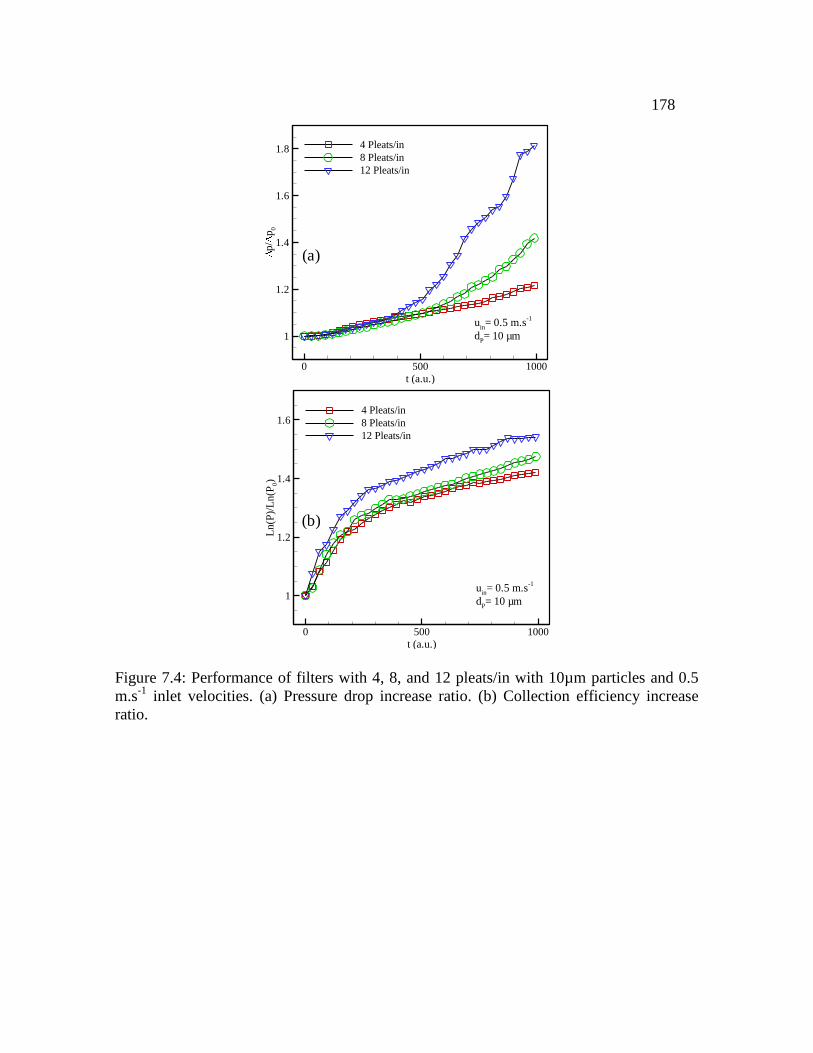
178

t (a.u.)

p/

p0

0 500 1000

1

1.2

1.4

1.6

1.8 4 Pleats/in

8 Pleats/in

12 Pleats/in

uin= 0.5 m.s

-1

dP= 10 µm

t (a.u.)

Ln

(P)/

Ln

(P0)

0 500 1000

1

1.2

1.4

1.64 Pleats/in

8 Pleats/in

12 Pleats/in

uin= 0.5 m.s

-1

dP= 10 µm

(a)

(b)

Figure 7.4: Performance of filters with 4, 8, and 12 pleats/in with 10µm particles and 0.5

m.s-1

inlet velocities. (a) Pressure drop increase ratio. (b) Collection efficiency increase

ratio.

179

(a)

(b)

Figure 7.5: Graphical demonstration for poly-dispersed dust deposition pattern inside

filters 4, 8 and 12 pleats/in with 1–10µm particles distribution for (a) 0.05 m.s-1

inlet

velocity and, (b) 0.5 m.s-1

inlet velocity.

180

t (a.u.)

p/

p0

0 50000 100000 150000

1

1.5

2

2.5

4 Pleats/in

8 Pleats/in

12 Pleats/in

uin= 0.05 m.s

-1

(a)

t (a.u.)

Ln

(P)/

Ln

(P0)

0 50000 100000 150000

1

2

34 Pleats/in

8 Pleats/in

12 Pleats/in

uin= 0.05 m.s

-1

(b)

t (a.u.)

p/

p0

0 50000 100000 150000

1

2

3

4

4 Pleats/in

8 Pleats/in

12 Pleats/in

uin= 0.5 m.s

-1

(c)

t (a.u.)

Ln

(P)/

Ln

(P0)

0 50000 100000 150000

1

1.5

2 4 Pleats/in

8 Pleats/in

12 Pleats/in

uin= 0.5 m.s

-1

(d)

Figure 7.6: Performance of filters with 4, 8, and 12 pleats/in with poly-dispersed particles

(a) Pressure drop increase ratio for 0.05 m.s-1

inlet velocity. (b) Collection efficiency

increase ratio for 0.05 m.s-1

inlet velocity. (c) Pressure drop increase ratio for 0.5 m.s-1

inlet

velocity. (d) Collection efficiency increase ratio for 0.5 m.s-1

inlet velocity.

181

CHAPTER 8 Overall Conclusions

This dissertation is intended to model the effects of micro-scale geometric parameters on

the performance of fibrous structures and propose a method to use them to study the effects

of the macro-scale geometric parameters on the performance of pleated filters. Our micro-

scale simulations (Chapters 2–4) are comprised of a series of computational fluid dynamics

calculations conducted in virtual fibrous geometries that resemble the internal micro-

structure of a fibrous medium. These simulations were conducted to isolate the effects of

each microstructural parameter (e.g., fiber diameter, fiber orientation, fiber cross-sectional

shape, and porosity) and study its influence of the performance of the filter medium. In our

macro-scale simulations (Chapters 5–7), the filter medium is treated as a lumped porous

material with its properties obtained via the results of the micro-scale simulations. The

macro-scale model is developed to simulate the unsteady-state performance of pleated

filters, and study the importance of their macro-scale dimensions (e.g., pleat shape, pleat

height, and pleat count).

While analytical expressions are available for the predicting performance of filters made

up of fibers with a unimodal distribution, there are few equally simple relations for

bimodal/multimodal filters. A series of numerical simulations were therefore formulated

for studying the performance of filter media with bimodal fiber diameter distributions. The

results were then utilized to establish an equivalent diameter for the bimodal media,

182

thereby taking advantage of the existing expressions for unimodal filters. Our results

indicate that the cube root relation of Tafreshi et al. (2009) offers the closest predictions

for the range of consideration for particle diameter, fiber number (mass) fractions, fiber

diameter ratio, and solid volume fraction (SVF). Another part of our micro-scale study was

conducted to better understanding of the influence of fibers’ in-plane and through-plane

orientations on the performance of fibrous media. Our results indicate that pressure drop of

common fibrous filters is independent of the in-plane orientation of the fibers, but decrease

with increasing the fibers’ through-plane orientation. More interestingly, it was found that

filters with higher through-plane fiber orientations have a higher Figure of Merit if

challenged with nano-particles. The Figure of Merit of these media, however, decreases as

the particle size increases, reversing the effect of fibers’ through-plane orientation. It was

also shown that when the diameter of the particles is comparable to that of the fibers,

collection efficiency increases with decreasing the fibers’ in-plane orientation, while the

pressure drop remains almost unchanged.

As mentioned, no mathematical formulations have yet been developed to predict the

performance of non-circular fibrous media. In this study, trilobal fibers with different

dimensions and aspect ratios were considered to study performance of filters made of such

fibers. More importantly, the above information was utilized to define an equivalent

medium with circular fibers. Our results indicate that the circumscribed circle of a trilobal

fiber can serve as an equivalent circular diameter, and thereby be used in the existing semi-

empirical correlations for predicting performance of filters with circular fibers. We have

183

also proposed easy-to-use expressions that can be used with our equivalent circumscribed

diameters for calculating the pressure drop of trilobal media.

While micro-scale simulations are accurate and most realistic, they are computationally

very expensive, and cannot be utilized to simulate a filter on scales comparable to its actual

dimensions. Therefore, we developed a novel macro-scale model that can incorporate

micro-scale information in cost-effective calculations performed for the filters in their

actual dimensions. Pleat optimization has been of particular interest in this study. We

considered three different classes of filters: 1) HEPA filters (performing as surface filters);

2) pre-filters (performing as depth filters); and 3) intermediate filters (performing at a level

between the above two extremes).

For HEPA pleated filters with the presence of dust surface deposition, it was found that the

rate of increase of pressure drop decreases with increasing the pleat count. Especially when

particles are sufficiently large, the dust cake tends to form deeper inside the pleated

channel when the pleat count is high. We also observed that rectangular pleats are

preferred over the triangular pleats when the particles are highly inertial, i.e., filtering high-

speed large particles.

To model pre-filters, a computationally affordable macro-scale method was developed to

simulate the instantaneous performance of these aerosol filters. Our results indicate that

increasing the number of pleats reduces the rate of increase of a filter’s pressure drop and

184

capture efficiency. Predictions of our model are compared against available experimental

data, and good agreement has been observed.

At last, we enhanced the above algorithms to model filters that do not necessarily perform

as a perfect depth or a perfect surface filter. For the case of mono-dispersed low-inertia

particles, more number of pleats always results in lower pressure drop and collection

efficiency increase. In contrast, when a filter encounters with highly inertial particles, then

more number of pleats causes the filter to clog faster. When particles are poly-dispersed in

size, then the aerosol contains higher mass fraction due to large size particles, and

therefore, fewer number of pleats shows better performance.

185

Literature Cited

186

References

Banks, D.O., 1987. Stokes flow through a system of parallel infinite cylinders with axes

oriented at angle top the direction of mean flow. Particulate Science and Technology 5,

339-353

Banks, D.O, Kurowski, G.J, Whitaker, S., 1990. Diffusion deposition on a fiber in non-

transverse flow. 2nd World congress: Particle Technology.

Batel, W., 1959. Chemie Ingenieur Technik, 31, 388.

Brown, R.C., 1993. Air filtration. Pergamon Press.

Brown, R.C. and Thorpe, A., 2001. Glass-fiber filters with bimodal fiber size distributions.

Power Technology. 118, 3.

Caesar, T., Schroth, T., 2002. The influence of pleat geometry on the pressure drop in deep

–pleated cassette filters. Filtration and Separation 39 (9), 48-54.

Chen, C.W., Huang1, S.H., Chiang, C.M., Hsiao, T.C., Chen, C.C., 2008. Filter quality of

pleated filter cartridges, Annual Occupation Hygiene, 52, 3, 207–212.

Chen, D.R., Pui, D.Y.H., Liu, B.Y.H., 1995. Optimization of Pleated Filter Designs Using

a Finite-Element Numerical Model. Aerosol Science and Technology 23 (4), 579-590.

Clague, S.D. and Phillips, R.J. (1997) A numerical calculation of the hydraulic

permeability of tree dimensional disordered fibrous media. Physics of Fluids. 9 (6), 1562.

Davies, C.N., 1973. Air Filtration. Academic Press, London.

Del Fabbro, L., Laborde, J.C., Merlin, P., Ricciardi, L., 2002. Air flows and pressure drop

modeling for different pleated industrial filters. Filtration and Separation 39 (1), 48-54.

Dhaniyala S., Liu, B.Y. H., 1999. “An asymmetrical, three-dimensional model for fibrous

filters. Aerosol Science and Technology 30 (4), 333-348.

Doganoglu, Y., Jog, V., Thambimuthu, K.V., Clift, R., 1978. Removal of fine particles

from gases in fluidized beds. Transactions of the Institution of Chemical Engineering 56:

296.

Drummond, J.E. and Tahir, M.I. (1984) Laminar viscous flow through regular arrays of

parallel solid cylinders. International Journal of Multiphase Flow. 10, 515.

187

Dullien, F.A.L., 1992. Porous Media, Fluid Transport and Pore Structure. Academic Press

Inc. 2nd

edition.

Friedlander, S.K., 2000. Smoke, Dust, and Haze: Fundamentals of Aerosol Dynamics, 2nd

edition Oxford University Press.

Fotovati, S., Tafreshi, H.V., Pourdeyhimi, B., 2010. Influence of fiber orientation

distribution on performance of aerosol filtration. Chemical Engineering Science. 65 (18):

5285-5293.

Fotovati, S., Hosseini, S.A., Tafreshi, H.V., Pourdeyhimi, B., 2011. Modeling

instantaneous pressure drop of pleated thin filter media during dust loading. Chemical

Engineering Science. 66: 4036–4046.

Fotovati, S., Tafreshi, H.V., Pourdeyhimi, B., 2012. Modeling instantaneous pressure drop

of pleated thin filter media during dust loading. Separation and Purification Technology

(submitted).

Happel, J., 1959. Viscous flow relative to arrays of cylinders. A.I.Ch.E. Journal 5 (2), 174-

177.

Henry, F.S., Ariman T., 1983. Particulate science and technology, 1, 1-20.

Hoffmann, A.C., Finkers, H.J., 1995. A relation for the void fraction of randomly packed

particle beds. Powder Technology 82 (2), 197-203.

Hosseini, S.A., Tafreshi, H.V., 2010. Modeling Permeability of 3-D Nanofiber Media:

Effects of Slip

Jackson, W.G. and James, F.D., 1986. The permeability of fibrous porous media. The

Canadian Journal of Chemical Engineering. 64, 364.

Jaganathan, S., Tafreshi, H.V. and Pourdeyhimi, B., 2008. On the Pressure Drop Prediction

of Filter Media with Bimodal Fiber Diameter, Powder Technology. 181, 89.

Kasper, G., Schollmeier, S., Meyer, J., 2010. Structure and density of deposits formed on

filter fibers by inertial particle deposition and bounce. Journal of Aerosol Science 41(12),

1167-1182.

Koponen, A., Kandhai, D., Hellen, E., Alava, M., Koekstra, A., Kataja, M., Niskanen, K.

Sloot, P., Timonen, J., 1998. Permeability of three dimensional random fiber webs.

Physical Review Letters 80(4), 716-719.

188

Kuwabara, S., 1959. The forces experienced by randomly distributed parallel circular

cylinders of spheres in a viscous flow at small Reynolds number. Journal of the Physical

Society of Japan 14 (4), 527-532.

Lamb, G.E.R., and Costanza, P.A., 1980. Influences of Fiber Geometry on the

Performance of Non-Woven Air Filters: 3. Cross-Sectional Shape, Text. Res. J. 50 (6) 362-

370.

Lee, K.W., Gieseke, J.A., 1980. Note on the approximation of interceptional collection efficiencies,

J. Aerosol Sci. 11, 335-341.

Lee, K.W., Liu, B.Y.H., 1982. Theoretical study of aerosol filtration by fibrous filters, Aerosol Sci.

Tech. 1, 147-161.

Li, A., Ahmadi, G., 1992. Dispersion and deposition of spherical-particles from point

sources in a turbulent chemical flow. Aerosol Science and Technology 16 (4), 209-226.

Liu, B.Y.H., Rubow, K.L., 1990. Efficiency, pressure drop and figure of merit of high

efficiency fibrous and membrane filter media, Fifth World Filtration Conference, Nice,

France (1990).

Lucke, T., Fissan, H., 1996. The prediction of filtration performance of high efficiency gas

filter elements, Chemical Engineering Science 51 (8), 1199-1208.

Lundstrom, S.T., Gebart, G.B., 1995. Effect of perturbation of fiber architecture on

permeability inside fiber tows. Journal of Composite Materials. 29, 424.

Macdonald, I.F., El-Sayed., M.S., Mow., K., Dullien F.A.L., 1979. Flow through porous-

media - ergun equation revisited. Industrial and Engineering Chemistry Fundamentals, 18

(3), 199-208.

Mattern, J.K., Deen, M.W., 2008. Mixing rules for estimating the hydraulic permeability of

fiber mixtures. AIChE Journal. 54, 32.

Papathanasiou T.D., 2001. The hydraulic permeability of periodic arrays of cylinders of

varying size. Journal of Porous Media. 4(4), 323.

Payet, S., 1991. Filtrationstationnaire et dynamique des aerosols liquids submicroniques,

These de l’universite Paris ХІІ4 oct., 150 p., rapport CEA-R-5589.

Pich, J., 1965. The filtration theory of highly dispersed aerosols, Staub Reinhalt. Luft. 5,

16-23.

Pich, J., 1966. In aerosol science C. N. Davis, Academic Press, New York.

http://apps.isiknowledge.com/full_record.do?product=WOS&search_mode=GeneralSearch&qid=6&SID=1DmMm6i872AN7@i8gaE&page=1&doc=6&cacheurlFromRightClick=no

189

Rebai, M., Prat, M., Meireles, M., Schmitz, P., Beclet, R., 2010. Clogging modeling in

pleated filters for gas filtration, Chemical Engineering Research and Design 88 (4A), 476-

486.

Rao, N., Faghri, M., 1988. Computer modelilng of aerosol filtration by fibrous filters.

Aerosol Science and Technology, 8 (2) 133-156.

Raynor, P.C., Kim, S.W., 2004. CFD modeling of filter fibers with non-circular cross-

sections, AAAR conference, Atlanta.

Raynor, P.C., Chae, S.J., 2005. The Long-Term Performance of Electrically Charged

Filters in a Ventilation System, Journal of Occupational and Environmental Hygiene, 1,

463–471.

Rumer, R.R., 1962. Proc. ASCE, Journal of Hydraulics Division, 88 (4) 147.

Rumpf, H., Gupte, A.R., 1971. Influence of porosity and particle size distribution in

resistance law of porous flow. Chemie Ingenieur Technik, 43 (6) 367.

Sanchez, J.R., Rodriguez, J.M., Alvaro, A., Estevez, A.M., 2007. The capture of fly ash

particles using circular and noncircular cross-section fabric filters, Environ. Prog. 26 (1)

50-58.

Schweers, E., Loffler F., 1994. Realistic modeling of the behaviour of fibrous filters

through consideration of filter structure. Powder Technology 80, 191-206.

Sirkar, K.K., 1975. Transport in packed beds at intermediate Reynolds numbers. Ind. Eng.

Chem. Fundam. 14: 73.

Spielman, L., Goren, S.L., 1968. Model for predicting pressure drop and filtration

efficiency in fibrous media, Environmental Science and Technology 2, 279.

Stechkina, I.B., 1969. Diffusion precipitation of aerosols in fiber filters, Dokl. Acad. Nauk. SSSR.

167, 1327.

Stechkina, I.B., Kirsch, A.A., Fuchs, N.A., 1969. Studies on fibrous aerosol filters- IV.

Calculus of aerosol deposition in model filters in the region of maximum penetration. Ann.

Ocup. Hyg. 12,1-8

Subrenat, A., Bellettre, J., Cloirec, P.L., 2003. 3-D numerical simulations of fows in a

cylindrical pleated filter packed with activated carbon cloth, Chemical Engineering

Science 58, 4965 – 4973.

190

Tafreshi H.V., Rahman M.S.A., Jaganathan S., Wang Q., Pourdeyhimi B., 2009.

Analytical Expressions for predicting permeability of bimodal fibrous porous media.

Chemical Engineering Science. 64, 1154.

Tahir, M. A., Tafreshi, H. V., 2009. Influence of fiber orientation on the transverse

permeability of fibrous media, Physics of Fluids 21, 083604.

Spurny, K.R., 1998. Advances in aerosol filtration, Lewis Publisher, CRC Press LLC: 471.

Thomas, D., Penicot, P., Contal, P., Leclerc, D., Vendel, J., 2001. Clogging of the fibrous

filters by solid aerosol particles experimental and modelling study. Chemical Engineering

Science 56 (11), 3549-3561.

Tien, C., 1989. Granular filtration of aerosols and hydrosols, Butterworths, Boston.

Tronville, P., Sala, R., 2003. Minimization of resistance in pleated-media air filter design:

empirical and CFD approach, HVAC&R Reasearch, 9, 1, 95-106.

Waghode, A.N., Hanspal, N.S., Wakeman, R.J., Nassehi, V., 2007. Numerical analysis

of medium compression and losses in filtration area in pleated membrane cartridge filters,

Chemical Engineering Comm., 194, 1053–1064.

Wakeman, R.J., Hanspal, N.S., Waghode, A.N., and Nassehi, V., 2005. Analysis of pleat

crowding and medium compression in pleated cartridge filters, Chemical Engineering

Research and Design, 83(A10), 1246–1255.

Wang, Q., Maze, B., Tafreshi, H.V., Pourdeyhimi, B., 2007. Simulating through-plane

permeability of fibrous materials with different fiber lengths. Modeling and Simulation in

Materials Science and Engineering 15(8), 855-868.

191

APPENDIX A: Granular Filtration

The three major particle capture mechanisms mentioned in Appendix A have been developed and

presented for fibrous media. To predict the capture mechanisms due to Diffusion in granular beds

for a single collector, we used the work of the following expression (Spurny, 1998):

2 34 /

DE g ε Pe (A1)

In above, Pe is the Peclet number and g ε is the correction factor. To obtain the capture

efficiency due to interception with Reynolds number less than 1, we used the following:

3 21 5RE . g ε R (A2)

The correction factor g ε for the range of granular collectors (previously deposited particles) in

this study is as following (Sirkar, 1975):

1 30 5

22 1 5 1 1 5 8 1 3 1 2 3 1

/.

g ε . ε . ε ε ε ε (A3)

Equation B3 is valid when the granular collector has 1Re , with cell porosity ε of greater than

0.33 and Peclet number greater than 1000. Finally, for the SFE due to inertial impaction, we used

the equation offered by Doganoglu (1978) and modified it for the range of our collector and

particles sizes:

2 89IE . Stk γ (A4)

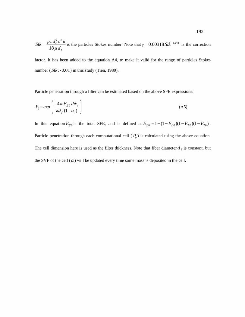
192

2

18

c

P P

f

ρ d c uStk

μdis the particles Stokes number. Note that

1 2480 00318 .γ . Stk is the correction

factor. It has been added to the equation A4, to make it valid for the range of particles Stokes

number ( 0 01Stk . ) in this study (Tien, 1989).

Particle penetration through a filter can be estimated based on the above SFE expressions:

00

4

(1 )

Σ c

f c

α E thkP exp

πd α (A5)

In this equation0ΣE is the total SFE, and is defined as

0 0 0 01 (1 )(1 )(1 )Σ D R IE E E E .

Particle penetration through each computational cell (0P ) is calculated using the above equation.

The cell dimension here is used as the filter thickness. Note that fiber diameter fd is constant, but

the SVF of the cell (α ) will be updated every time some mass is deposited in the cell.

193

VITA

Shahryar Fotovati

Education:

PhD, Mechanical and Nuclear Engineering

Virginia Commonwealth University. (Jan. 2009–March 2012)

Dissertation: Effects of Micro and Macro-Scale Geometrical Parameters on

Performance of Pleated Aerosol Filters.

M.Sc., Mechanical Engineering

Shiraz University. (Sep. 2004–Sep. 2007)

Thesis: Analysis and Control of Dynamic Stall on an Airfoil in 2-D Compressible

Turbulent Flows

B.Sc., Mechanical Engineering

Persian Gulf University. (Sep. 1996–May 2001)

Journal Publications:

1. S. Fotovati, H.V. Tafreshi, 2012, Pleated Filters Performance under Realistic dust

load conditions with poly-dispersed particles distribution; Effects of Depth and

Surface Deposition, (to be submitted).

2. B. Emami, S. Fotovati , H.V. Tafreshi, 2011. Effects of Fiber Orientation on

Permeability of Fibrous Media to Power-Law Fluids. Chemical Engineering Science

(under review).

3. S. Fotovati, H.V. Tafreshi, B. Pourdeyhimi, 2011. A Macro-scale Model for

Simulating Pressure Drop and Collection Efficiency of Pleated Filters over Time.

Separation and Purification Technology (under review).

194

4. S. Fotovati, S.A. Hosseini, H.V. Tafreshi, and B. Pourdeyhimi, 2011. Modeling

Instantaneous Pressure Drop of Pleated Thin Filter Media during Dust Loading.

Chemical Engineering Science, 66, 4036-4046.

5. S. Fotovati, H.V. Tafreshi, and B. Pourdeyhimi, 2011. Analytical Expressions for

Predicting Performance of Aerosol Filtration Media Made up of Trilobal Fibers.

Journal of Hazardous Materials, 186 (2), 1503-1512.

6. S. Fotovati, H.V. Tafreshi, and B. Pourdeyhimi, 2010. Influence of Fiber

Orientation Distribution on Performance of Aerosol Filtration. Chemical

Engineering Science, 65 (18), 5285-5293.

7. S. Fotovati, H.V. Tafreshi, et al., 2010. Analytical Expressions for Predicting

Capture Efficiency of Bimodal Fibrous Filters. Journal of Aerosol Science, 41 (3),

295-305.

Selected Conferences:

S. Fotovati, H.V. Tafreshi, and B. Pourdeyhimi. Transient Modeling of Dust-

Loaded Pleated Air Filters. American Filtration and Separation Society, June 2012,

Boca Raton, FL.

S. Fotovati, H.V. Tafreshi, and B. Pourdeyhimi. Transient Modeling of Dust-

Loaded Pleated Air Filters. American Filtration and Separation Society, May 9-12,

2011, Louisville, KY.

S. Fotovati, H.V. Tafreshi, and B. Pourdeyhimi. Effect of Fiber Orientation

Distribution on Filter Performance. American Filtration and Separation Society,

March 22-25, 2010, San Antonio, TX.

S. Fotovati, H.V. Tafreshi, B. Pourdeyhimi. Two-dimensional Modeling of

Nanoparticle Collection Efficiency in Bimodal Filters. American Filtration and

Separation Society, May 4-7, 2009, Minneapolis, MN.

195

Computational and Programming Skills

CFD Modeling: Turbulence, Aerodynamics, Discrete-Phase and Multi-Phase flows,

Porous Media.

Mesh Generation using Algebraic Model, or software.

Strong programming skills with: C++, FORTRAN, MATLAB, UDF.

Software packages: ANSYS-Fluent, GAMBIT, Flex-PDE, GeoDict, TECPLOT, MS

Office.

Experienced: AutoCAD, MATHEMATICA, Linux and Windows OS.

Familiarity: CFX, SOLIDWORK, ICEM CFD, R.

Honors and Awards:

Winner of the Best Technical Merit award in semiannual meeting IAB-NCRC (Jun.

2011).

Winner of VCU Dissertation Scholarship-award (Fall 2011).

Member of Honor Society of Phi Kappa Phi (2010-Present).

PhD GPA: 4.0 out of 4.0

Documents

THE EFFECTS OF MICRO- AND MACRO-SCALE GEOMETRIC PARAMETERS …