Ann. Geophys., 30, 695–701, 2012www.ann-geophys.net/30/695/2012/doi:10.5194/angeo-30-695-2012© Author(s) 2012. CC Attribution 3.0 License.

AnnalesGeophysicae

The emission of oxygen green line and density of O atom determinedby using ISUAL and SABER measurements

H. Gao1,2, J.-B. Nee2, and J. Xu1

1State Key Laboratory of Space Weather, CSSAR, Chinese Academy of Sciences, Beijing, China2Department of Physics, National Central University, Jhongli, Taiwan, China

Correspondence to:J.-B. Nee (jbnee@phy.ncu.edu.tw)

Received: 5 November 2011 – Revised: 28 March 2012 – Accepted: 31 March 2012 – Published: 19 April 2012

Abstract. Emissions of the 557.7 nm green line airglow ob-served by the ISUAL (Imager of Sprites and Upper Atmo-spheric Lightning) instrument on board the FORMOSAT-2satellite in May and November 2008 are studied here to de-rive the density distributions of the atomic oxygen by usingatmospheric parameters from MSISE-00 model and TIMED(Thermosphere Ionosphere Mesosphere Energetics and Dy-namics)/SABER (Sounding of the Atmosphere using Broad-band Emission Radiometry) measurements. The May obser-vations were made in 10 days from a fixed orbit of longitude(100◦ E) with the results showing emission rate and O atomdensity both peaked at heights of about 90 km over 10◦ to 20◦

latitudes in the Northern Hemisphere (NH). In the SouthernHemisphere (SH), the emission rate and density of O atomare both low compared with those in NH. In November, theobservations were made as the satellite traveled over all 14orbits around the earth, covering all longitudes and latitudesof 25◦ S–45◦ N. Strong peaks of emission rates and O atomsare found at heights of about 95 km in the mid-latitudes inboth hemispheres. In the equator, the airglow layer has aweaker emission rate but with higher altitude compared withthose of mid-latitudes. In the lower and upper mesosphereat heights below 85 km and above 105 km, there are moreO atoms in the equatorial regions than in the mid-latitudes.And there is a good correlation between the O atom and thetemperature structure. A comparison with O atom distribu-tion derived from OH airglow observed by TIMED/SABERat about the same time shows similar results.

Keywords. Atmospheric composition and structure (Air-glow and aurora; Middle atmosphere – composition andchemistry; Pressure, density, and temperature)

1 Introduction

The green line emission at the wavelength 557.7 nm (here-inafter referred to as 558 nm) arising from the O(1S–1D) tran-sition is one of the prominent nightglow features in the meso-sphere. The production of the excited oxygen atom O(1S) ofan energy 4.2 eV was first proposed by Chapman in terms ofa three body recombination of O atoms (Bates, 1988). How-ever, a two-step mechanism involving an excited state of O2was proposed later by Barth (1961). The Barth Mechanisminvolves the following steps:

O+ O+ M → O∗

2 + M (R1)

O+ O∗

2 → O(1S) + O2. (R2)

Studies of the green line and O atoms by various measure-ments have generally favored the Barth mechanism. Previousground based and rocket measurements have provided usefulinformation about the green line airglow, they are limited inspatial and time domains. The latest development of spaceinstruments such as WINDII (Wind Imaging Interferometer)and SABER have provided extended information about theglobal and temporal variations of the airglow. For exam-ple, Zhang and Shepherd (1999) have shown green line had amidnight enhancement and peaked in mid latitudes based onWINDII observations. In the same study, they have found theOH Meinel band airglow peaked in the equator. In fact, OHairglow is also related to the chemistry of O atom throughozone by the chemical reaction

H + O3 → OH∗+ O2 (R3)

with O3 produced from O atom by the three body recombi-nation process:

O+ O2 + M → O3 + M. (R4)

Published by Copernicus Publications on behalf of the European Geosciences Union.

696 H. Gao et al.: Emission of oxygen green line and density of O atom

Therefore, the measurements of OH airglow can also pro-vide information about abundance of O atom. The differ-ence in the latitudinal distributions of the O(1S) and OH air-glow reveals dynamic features governing their global distri-butions. A study of O atom from OH airglow observed byTIMED/SABER instruments is also studied in this paper tocompare with results from green line airglow.

McDade et al. (1986) has discussed the mechanism for theproduction of the green line based on Reactions (R1) and(R2) and derived an expression of the emission rate with thefollowing equation

V558nm= A558nm

[O

(1S

)](1)

=A558nmκ1 [O]3 [M]{(

A(1S

)+ κ5 [O2]

)(C

′(0)+C′(1) [O] +C

′(2) [O2])}

where [] means number density,V558nm is the emission ratein photons cm−3 s−1, [M] is the density of air includingboth O2 and N2. The rate constant with the three bodyrecombination of O atoms isκ1 = 4.7× 10−33(300/T )2,and the quenching rate of O

(1S

)by O2 is κ5 = 2.32×

10−12exp((−812− 1.82× 10−3T 2)/T ) (Capetanakis et al.,1993). In our study, the Einstein coefficientsA558nm andA(1S) are set as 1.26 s−1 and 1.34 s−1, respectively, whichwere given by Martin et al. (1999) and used in the study ofNakayama et al. (2006). ConstantsC

′(0), C′(1) andC

′(2) aregiven in McDade (1986).

From Eq. (1), we findV558nm is proportional to O atomto a cubic power: [O]3. The ratesk1 andk5 are temperaturedependent such that the net emission rate is inversely relatedto the temperature while O atom is positively related to thetemperature of the atmosphere. By measuring the emissionrate at 558 nm, we should be able to derive the density ofO atom with knowledge of the atmospheric temperature anddensity.

As we have discussed, the O atom can be studied by emis-sions of OH and O(1S). In the past, Russell et al. (2003, 2004)have investigated the O atom distribution based on the greenline data from WINDII measurements. Smith et al. (2010)have extensively studied the characteristic height of O atomover a region of 80–95 km by using the OH airglow measuredby SABER instrument.

In this paper, we will study the green line and O atom dis-tributions based on measurements made by the ISUAL in-strument on board the FORMOSAT-2 satellite. In the nextsection, we will discuss the ISUAL instrument and measure-ments of the green line. In the third section, results of OI558emission rate and distributions of O atoms are presented.Results of O atoms by using different atmospheric param-eters and the derivation by using SABER OH airglow arediscussed. Finally, a summary is given in the last section.

2 Instrument description and data processing

The ISUAL instrument on board the FORMOSAT-2 satel-lite was launched in May 2004 to a sun-synchronous orbit of890 km with an inclination angle of 98.9◦. The satellite has14 orbits a day circling around the earth and can observe thesame region of the atmosphere at a fixed latitude and longi-tude at the same local time. This type of observation providesa unique opportunity to study the upper atmosphere in detailcompared with other non-sun-synchronous satellites whichrequire months to return to the same local time at the sameplace.

The ISUAL instrument includes a CCD camera whichlooks through one of six interference filters to observe theatmospheric emissions in limb view (Nee et al., 2010). Inthis research, Filter #4 at 558 nm (FWHM 6 nm) is used tocapture images of the green line airglow layer. The CCDtakes 20 to 41 pictures of the atmosphere as the satellite trav-els along a specific orbit by looking out a distant window of3300 km away. Each CCD picture has 524 (horizontal)×

128 (vertical) pixels corresponding to a window of 1200 km(width)× 270 km (height) of the upper atmosphere. A spatialresolution of about 2.14 km per pixel has been determinedfrom the calibration.

Over the period of 7–16 May 2008, the green line wasobserved along the #10 orbit every night at midnight (localtime). Forty one pictures were taken as the satellite traveledalong this orbit. As an example, Fig. 1a gives a combined im-age of all 41 pictures to show a single layer of O(1S) airglowobserved on 10 May 2008. The observations started from theSH and ended in NH, covering latitudes of∼11◦ S–20◦ N.The orbit 10 covers longitudes of about 98◦ E–107◦ E (brieflydesignated as 100◦ E in this paper). For the second greenline observations for 1–2 November 2008, images have beentaken along every orbit with orbits on 1 November from #9to 14 and on 2 November from #1 to 8 and also #10. There-fore, these two day observations in November have coveredall regions around the earth. The orbits which the satellitetraveled to observe 558 nm airglow in this period are shownin Fig. 1b where one point on a track represents that one pic-ture was recorded there. There are 21 pictures taken alongevery orbit (except the #14 orbit on Nov.1 and the #7 orbiton 2 November in which 20 pictures were taken because oforbit connectivity. In addition, on 2 November, the #10 orbitrecorded 41 pictures).

By using an “onion-peel” process, the green line volumeemission rate profiles can be retrieved from the images as de-scribed in Nee et al. (2010). Although there are 512 columnpixels in one picture, we just use the 10 central column pix-els to produce a profile of the emission rate. These emissionrates are then used to calculate the O atom distributions byusing Eq. (1) described in the first section.

The SABER instrument on board the TIMED satellite waslaunched in December 2001 to an altitude of 625 km with aninclination angle 74.1◦. The satellite travels around the earth

Ann. Geophys., 30, 695–701, 2012 www.ann-geophys.net/30/695/2012/

H. Gao et al.: Emission of oxygen green line and density of O atom 697

4 

Over the period of May 7－16 2008, the green line was observed along the # 10 orbit every night

at the midnight hour (local time). Forty one pictures were taken as the satellite traveled along this orbit.

As an example, Fig. (1a) gives a combined image of all 41 pictures to show a single layer of O(1S)

airglow observed on May 10 2008. The observations started from the SH and ended in NH covering

latitudes of ～11°S－20°N. The orbit 10 covers longitudes of about 98°E－107°E (briefly designated as

100°E in this paper). For the second green line observations for Nov. 1－2 2008, images have been taken

along every orbit with orbits on Nov.1 from # 9 to 14 and on Nov.2 from #1 to 8 and also #10. Therefore,

these two day observations in November have covered all regions around the earth. The orbits which the

satellite traveled to observe 558 nm airglow in this period are shown in Fig. (1b) where one point on a

track represents that one picture was recorded there. There are 21 pictures taken along every orbit

(except the #14 orbit on Nov.1 and the #7 orbit on Nov. 2 in which 20 pictures were taken because of

orbit connectivity. In addition, on Nov. 2, the #10 orbit recorded 41 pictures.).

By using an ‘onion-peel’ process, the green line volume emission rate profiles can be retrieved

from the images as described in Nee et al. (2010). Although there are 512 column pixels in one picture,

we just use the 10 central column pixels to produce a profile of the emission rate. These emission rates

are then used to calculate the O atom distributions by using Eq. (1) described in the first section.

Figure 1 (a) An image of a layer of O(1S) airglow measured on May 10 2008. (b) The latitudes and

longitudes of ISUAL orbits. For Nov. 1－2 2008, one point in the figure represents one picture of

the OI558 nm airglow emission was taken there.

Fig. 1. (a) An image of a layer of O(1S) airglow measured on10 May 2008. (b) The latitudes and longitudes of ISUAL orbits.For 12 November 2008, one point in the figure represents one pic-ture of the OI558 nm airglow emission was taken there.

by about 15 orbits and takes about 60 days to cover the wholeearth in every 24 h local time. The SABER instrument is a10 channel infrared radiometer designed to measure the radi-ation, energy and structures of the MLT region (mesosphereand lower thermosphere). SABER observations cover fromthe winter hemisphere 53◦ to the summer hemisphere 83◦.For every 58 s, SABER scans from 0 to 180 km to take at-mospheric parameters including temperature, density, ozonedensity and OH airglow at the emission wavelengths 1.6 µmand 2.0 µm (see Russell et al., 1999). In this paper, we usethe SABER 2.0 µm OH emission and ozone to derive the Oatom by using the method introduced by Smith et al. (2010).

3 Results

3.1 558 nm emission rate

As an example, Fig. 2 shows the scattered diagrams of theheight distributions of the emission rates derived from all 41images measured on 10 May. Each image can derive a heightprofile separated by about 0.7◦ latitudes from the neighbor-ing images. The black line in Fig. 2 is the average profileof all 41 data. From this figure we can see all data can fit aGaussian distribution over a height range of 80–110 km withan average peak height of 92 km. As shown in Fig. 2, thepeak height is quite stable for all data despite that the emis-sion intensity can vary by about a factor of two. Such stableheight distribution was not observed in OH airglow (Nee etal., 2010).

The peak height of O(1S) airglow has been reported bymany groups using different instruments (Zhang and Shep-

5 

The SABER instrument on board the TIMED satellite was launched in December, 2001 to an

altitude of 625 km with an inclination angle 74.1°. The satellite travels around the earth by about 15

orbits and takes about 60 days to cover the whole earth in every 24 hours local time. The SABER

instrument is a 10 channel infrared radiometer designed to measure the radiation, energy and structures

of the MLT region (mesosphere and lower thermosphere). SABER observations cover the winter

hemisphere from 53° to the summer hemisphere 83°. For every 58 seconds, SABER scan from 0 to 180

km to take atmospheric parameters including temperature, density, ozone density, and OH airglow at the

emission wavelengths 1.6 μm and 2.0 μm (see Russell et al., 1999). In this paper, we have used the

SABER 2.0 μm OH emission and ozone to derive the O atom by using the method introduced by Smith

et al. (2010).

3 Results 3.1 558 nm emission rate

As an example, Fig. 2 shows the scattered diagrams of the height distributions of the emission

rates derived from all 41 images measured on May 10. Each image can derive a height profile separated

by about 0.7° latitudes from the neighboring images. The black line in Fig. 2 is the average profile of all

41 data. From this figure we can see all data can fit a Gaussian distribution over a height range of 80－

110 km with an average peak height of 92 km. As shown in Fig. 2, the peak height is quite stable for all

data, despite the emission intensity can vary by about a factor of two. Such stable height distribution

was not observed in OH airglow (Nee et al., 2010).

70

75

80

85

90

95

100

105

110

115

120

0 20 40 60 80 100 120 140 160 180

V558nm (photons cm-3 s-1)

Alti

tude

(km

)

41 profiles in orbit 10 on 10 May

 

Figure 2 Forty one scattered profiles of OI558 nm volume emission rate retrieved from images Fig. 2. Forty one scattered profiles of OI558 nm volume emissionrate retrieved from images taken from orbit 10 on 10 May 2008.The 41 data are marked by different colors and symbols with theaverage profile in black solid line.

herd, 1999; Liu et al., 2008a; Yee et al., 1997; Skinner etal., 1998) and rocket measurements (Melo et al., 1996). Theaverage peak height seems to be about 96 km. Our May ob-servation shows a lower peak height of about 92 km. The dif-ference may be related to the variations of airglow with thetime, season and dynamics, as discussed extensively in Liuet al. (2008a) by using WINDII measurement. Long termstudies show O(1S) can vary between 84–104 km dependingon the season and time (Liu et al., 2008a). The HRDI (HighResolution Doppler Imager) instrument also shows seasonaland local time variations of green line airglow (Skinner et al.,1998).

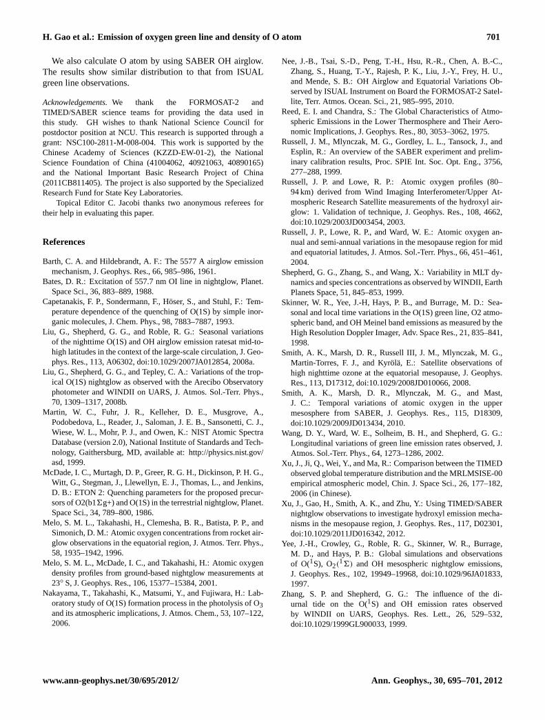
A contour diagram for green line in terms of height ver-sus latitude can be made by averaging the emission rate ingrids of 5 degree latitudes as shown in Fig. 3a and b for Mayand November data. For May data the measurements weremade over a fixed longitude of about 100◦ E and latitudes of10◦ S–20◦ N. We find the peak height is about 92 km and thepeak emission in the NH is higher than that in the SH. ForNovember data, the measurements were made over the lati-tudes of 25◦ S–45◦ N but over all longitudes. The results ofaveraging all longitudes gives a global distribution, showinggreen line emission at the equator is high in altitude but weakin intensity compared with those of mid-latitudes which havelower peak heights but stronger emission intensity. The twomid-latitude maxima are at about 95 km at 25◦ S and 93 kmat 30◦ N with emission rates of 180 photons cm−3 s−1 and240 photons cm−3 s−1, respectively. Our results are basicallyconsistent with WINDII/UARS data of Zhang and Shepherd(1999) who have shown OI558 nm emission rates are lownear equator but high in the mid-latitudes for March 1992,

www.ann-geophys.net/30/695/2012/ Ann. Geophys., 30, 695–701, 2012

698 H. Gao et al.: Emission of oxygen green line and density of O atom

7 

-10 -5 0 5 10 15 2080

85

90

95

100

105

110

(b) V558nm (Photons cm-3 s-1) in Nov.(a) V558nm (Photons cm-3 s-1) in May

Altit

ude

(km

)

Latitude (deg)

0.000 40.00 80.00 120.0 160.0 200.0

-20 -10 0 10 20 30 4080

85

90

95

100

105

110

Latitude (deg)

0.000 64.00 128.0 192.0 248.0

 

Figure 3 The height-latitudinal distributions of green line emission rates observed by ISUAL in (a) May

2008 along orbit 10 (longitude～100°E）and (b) November 2008 averaging over all longitudes.

We notice that the global measurement reveals a symmetric distribution with respect to the

equator with the NH and SH peaks appearing as mirror images of each other as shown in Fig. (3b).

The symmetric distribution is also found in WINDII observation as shown in Zhang and Shepherd

(1999).

3.2 Derivation of O atom density based on MSIS model

As discussed above, we can use the 558 nm emission rate to derive the density distribution of O

atoms by using Eq. (1) with the knowledge of background atmospheric temperature and density. Russell

et al. (2003, 2004) have used the MSIS model to calculate O atom based on WINDII 558 nm data. We

also used MSISE-00 model to derive O atom by using ISUAL OI 558 nm emission rate. We have

selected the model calculations by using the same time and geological coordinates corresponding to the

observations. Fig. (4a) shows 41 scattered diagrams of height distributions of O atom measured along

the longitude 100oE corresponding to the emissions shown in Fig. (3a).The average profile is shown as

the solid black line. From Fig. (4a), we can see O atom on 10 May has a peak at about 92 km and a

minimum at about 112 km. O atom increases with altitude above 112 km reaching a secondary peak

above 120 km. However, we must be reminded there are also more errors at height below 80 km and

above 110 km where emission rates are low and standard deviations are high.

Fig. 3. The height-latitudinal distributions of green line emissionrates observed by ISUAL in(a) May 2008 along orbit 10 (longitude∼100◦ E) and(b) November 2008 averaging over all longitudes.

December 1992, and February 1993 at midnight conditions.We also find the magnitudes of the emission rates of ISUALand WINDII data are close (Shepherd et al., 1999; Wang etal., 2002; Liu et al., 2008b).

We notice that the global measurement reveals a sym-metric distribution with respect to the equator with the NHand SH peaks, appearing as mirror images of each other asshown in Fig. 3b. The symmetric distribution is also foundin WINDII observation as shown in Zhang and Shepherd(1999).

3.2 Derivation of O atom density based on MSIS model

As discussed above, we can use the 558 nm emission rate toderive the density distribution of O atoms by using Eq. (1)with the knowledge of background atmospheric temperatureand density. Russell et al. (2003, 2004) used the MSIS modelto calculate O atom based on WINDII 558 nm data. We alsoused MSISE-00 model to derive O atom by using ISUALOI 558 nm emission rate. We have selected the model cal-culations by using the same time and geological coordinatescorresponding to the observations. Figure 4a shows 41 scat-tered diagrams of height distributions of O atom measuredalong the longitude 100◦ E corresponding to the emissionsshown in Fig. 2. The average profile is shown as the solidblack line. From Fig. 4a we can see O atom on 10 May hasa peak at about 92 km and a minimum at about 112 km. Oatom increases with altitude above 112 km, reaching a sec-ondary peak above 120 km. However, we must be remindedthere are also more errors at heights below 80 km and above110 km where emission rates are low and standard deviationsare high.

Based on results shown in Fig. 4a, the O atom distributioncan be fitted with a Chapman profile as described in Eq. (2)below. This is the way Reed and Chandra (1975) and Melo

8 

 

Figure 4 (a) Height distributions of O atom derived from forty-one 558 nm emission rates observed

along orbit 10 on May 10 2008 (in different symbols and colors). The solid black line represents the

average profile. (b) two profiles of specific latitudes and longitudes (7.2°S, 104°E) and (12.2°N,

100°E) (doted lines), and their simulated results (solid lines) by using Eq.(2).

Based on results shown in Fig. (4a), the O atom distribution can be fitted with a Chapman

profile as described in Eq. (2) below. This is the way Reed and Chandra (1975) and Melo et al.

(2001) have reported their distributions for the mesospheric O atoms.

[O]z =[O]maxexp{0.5[1-(z-hmax)/w]–exp[- (z-hmax)/w]} (2)

In Eq. (2), [O]z is the atomic oxygen density at an altitude z; [O]max and hmax are the peak density

and height of the atomic oxygen respectively, and w is the width of profile.

By using Eq. (2), we have simulated the O atom distribution in 70－120 km by a least-square

fit. In Fig. (4b), the dots are the height distributions of two observations at (7.2°S, 104°E) and

(12.2°N, 100°E) and solid lines for the fitting results. In this figure, we find the height distributions

of O atoms in the NH and SH are different, which should result from slightly un-symmetric

distribution of airglow intensities in NH and SH as can be seen in Fig. (3a).

It is known that MSISE-00 as an empirical model provides a good representation of the

atmosphere in the region of middle to lower mesosphere but is not very accurate in the mesopause

region (Xu et al., 2006). Recently by comparing the TIMED data with MSISE-00, Xu et al. (2006)

have reported the deviations of MSISE-00 model. They also found inconsistency for cases of

temperature inversions and some small scale deviations at different seasons.

3.3 Mesospheric temperatures based on SABER observations

Fig. 4. (a) Height distributions of O atom derived from forty-one558 nm emission rates observed along orbit 10 on 10 May 2008 (indifferent symbols and colors). The solid black line represents theaverage profile.(b) Two profiles of specific latitudes and longitudes(7.2◦ S, 104◦ E) and (12.2◦ N, 100◦ E) (doted lines), and their sim-ulated results (solid lines) by using Eq. (2).

et al. (2001) reported their distributions for the mesosphericO atoms:

[O]z=[O]maxexp{0.5[1−(z−hmax)/w]−exp[−(z−hmax)/w]}.

(2)

In Eq. (2), [O]z is the atomic oxygen density at an altitudez; [O]max andhmax are the peak density and height of theatomic oxygen, respectively, andw is the width of profile.

By using Eq. (2), we have simulated the O atom distribu-tion in 70–120 km by a least-square fit. In Fig. 4b, the dotsare the height distributions of two observations at (7.2◦ S,104◦ E) and (12.2◦ N, 100◦ E) and solid lines for the fittingresults. In this figure, we find the height distributions of Oatoms in the NH and SH are different, which should resultfrom slightly un-symmetric distribution of airglow intensi-ties in NH and SH, as can be seen in Fig. 3a.

It is known that MSISE-00 as an empirical model pro-vides a good representation of the atmosphere in the regionof middle to lower mesosphere but is not very accurate in themesopause region (Xu et al., 2006). Recently by comparingthe TIMED data with MSISE-00, Xu et al. (2006) have re-ported the deviations of MSISE-00 model. They also foundinconsistency for cases of temperature inversions and somesmall scale deviations at different seasons.

3.3 Mesospheric temperatures based on SABERobservations

We have employed TIMED/SABER temperature and densitydata as an alternative to the MSIS model for the calculationsof O atom. One of the problems of using SABER mea-surements with ISUAL is related to their different orbits andobservation strategies. It is rare that both satellites will belocated at the same region to observe the same atmosphere

Ann. Geophys., 30, 695–701, 2012 www.ann-geophys.net/30/695/2012/

H. Gao et al.: Emission of oxygen green line and density of O atom 699

10 

-10 -5 0 5 10 15 2080

85

90

95

100

105

110

Altit

ude

(km

)

Latitude (deg)

154.0 170.0 186.0 202.0 218.0 234.0 250.0

(a) Temperature (K) in May (b) Temperature (K) in Nov.

-20 -10 0 10 20 30 4080

85

90

95

100

105

110

Latitude (deg)

165.0 180.0 195.0 210.0 225.0 240.0 255.0

 

Figure 5 SABER temperatures correspond to the same orbital conditions for (a) May and (b)

November airglow observations.

3.4 O atom based on SABER observations

By using SABER temperature and density data in Eq. (1), we have calculated O atom

distributions for May and November with results shown in Fig. 6. Fig. (6a) indicates a layer of O

atoms exists in May at 85－95 km with the peak height increasing with latitude even though the

emission rate is relatively unchanged in height distribution as shown in Fig. (3a). This difference

should be attributed to the temperature distribution as shown in Fig. (5a). The number density of O

atoms in the NH is more and higher than those in the SH. A maximum of O atom appears at 10°N at

90 km. Besides these trends, there is a low value of O atom at about 95 km at 10°S in the SH related

with the temperature conditions shown in Fig. (5a).

In November, O atom shows several maxima and minima in different heights and latitudes.

Below 85 km, more O atoms are found at the equator than other regions. In the mid-latitudes there are

two minima found at about 25°S/N. In the region of 85－100 km, there is a peak of O atom at about 93

km at 30°N. The corresponding peak in the SH should lie at 30° but was partially cut in the diagram.

These two mid-latitude peaks form mirror images similar to the emission double shown in Fig. (3b). A

major peak of O atom is located at about 10°N at 110 km, and a secondary peak at 10°S at 104 km. The

last two peaks lying above 100 km are correlated with the temperature structure in this region as can be

seen in Fig. (5b).The secondary peak at 10°S may be a split from the major peak.

In terms of absolute number density, O atoms in May or November are both in the level of 1011

cm-3 which is close to other results reported in the literatures (e.g. Smith, et al., 2010; Russell et al.,

2003). We also calculated the volume mixing ratio (vmr) of O. The altitude-latitude distribution of the

Fig. 5. SABER temperatures correspond to the same orbital condi-tions for(a) May and(b) November airglow observations.

at the same time. Fortunately, SABER observations weremade around midnight in both periods of 7–16 May and 1–2 November 2008. We have therefore selected SABER ob-servations for heights of 80–110 km during 7–16 May 2008with the longitudes between 90◦ E and 110◦ E and during 1–2 November 2008 in all longitudes in the time interval of−02:00 LT to 02:00 LT local time to construct bins of 5 de-gree latitudes. We then used ISUAL OI 558 nm emission rateto calculate O atom density within these bins.

We will first look at the SABER temperature data since itis an important parameter in the calculations. Figure 5 showscontour diagrams of SABER temperatures for both May andNovember in 2008. We find from Fig. 5a the mesopause inMay is located at about 97 km with a low temperature ofabout 160 K. Below the mesopause, there is a warm layerwith a local temperature maximum of about 220 K at about83 km at 10◦ S. The height of this warm layer increasesto 92 km at 20◦ N. Higher temperatures also appear above105 km.

For November, the temperature structure shows a complexpattern in terms of multiple highs and lows. The mesopauseheight is at 95 km over the equatorial region and increases toabout 100 km at mid-latitudes in the SH and NH as shown inFig. 5b. In the lower mesosphere at about 85 km, the tem-perature in the equatorial region is higher than those in themid-latitudes. But in the upper mesosphere at heights 100–110 km, there is a warm layer corresponding to the thermo-sphere. In November, high temperatures in the mesospherecan be found in three regions: 81 km over the equator, 90 kmat both 25◦ S and 30◦ N. The highest temperature appearsabove the mesosphere at 110 km at 10◦ N.

By comparing Fig. 5b with Fig. 3b, we can see the stronger558 nm airglow layer lies near the mesopause. We must bereminded that emission is negatively correlated and O atomis positively correlated with temperature as given in Eq. (1),so that peak emission and O atom are correlated with coldand warm regions, respectively.

3.4 O atom based on SABER observations

By using SABER temperature and density data in Eq. (1), wehave calculated O atom distributions for May and Novemberwith results shown in Fig. 6. Figure 6a indicates a layer ofO atoms exists in May at 85–95 km with the peak height in-creasing with latitude even though the emission rate is rela-tively unchanged in height distribution as shown in Fig. 3a.This difference should be attributed to the temperature distri-bution as shown in Fig. 5a. The number density of O atoms inthe NH is more and higher than those in the SH. A maximumof O atom appears at 10◦ N at 90 km. Besides these trends,there is a low value of O atom at about 95 km at 10◦ S in theSH related to the temperature conditions shown in Fig. 5a.

In November, O atom shows several maxima and min-ima in different heights and latitudes. Below 85 km, moreO atoms are found at the equator than other regions. In themid-latitudes there are two minima found at about 25◦ S/N.In the region of 85–100 km, there is a peak of O atom at about93 km at 30◦ N. The corresponding peak in the SH shouldlie at 30◦ but was partially cut in the diagram. These twomid-latitude peaks form mirror images similar to the emis-sion double shown in Fig. 3b. A major peak of O atom islocated at about 10◦ N at 110 km, and a secondary peak at10◦ S at 104 km. The last two peaks lying above 100 km arecorrelated with the temperature structure in this region as canbe seen in Fig. 5b. The secondary peak at 10◦ S may be a splitfrom the major peak.

In terms of absolute number density, O atoms in May orNovember are both in the level of 1011 cm−3 which is closeto other results reported in the literatures (e.g. Smith et al.,2010; Russell et al., 2003). We also calculated the volumemixing ratio (vmr) of O. The altitude–latitude distribution ofthe vmr below 100 km is very similar to the calculations ofSmith et al. (2010) who used SABER OH(2.0 µm) airglowto derive the O atom density and mixing ratio. In addition,our results indicate that the O atom at 10◦ N (109 km) hasa mixing ratio about 0.4 compared with less than 0.3 at allother latitudes and heights.

3.5 Discussion

Following Smith et al. (2008, 2010) and using the new co-efficients given by Xu et al. (2012), we also calculated theO atoms in the 80–100 km height region based on SABEROH(2.0 µm) airglow emission rate and ozone density mea-sured in the period of 7–16 May 2008 in−02:00–02:00 LTand in longitudes 90◦ E–110◦ E. Another calculation hasbeen made for 1–2 November 2008 at−02:00–02:00 LT butover all longitudes. The altitude–latitude distribution of theO atom retrieved from SABER May data shows O atomspeaks over the latitudes 10◦ S–20◦ N and heights 80–100 kmsimilar to what are displayed in Fig. 6a. There are more Oatom in the NH than the SH and the peak height increasesin general toward mid-latitudes in the NH. SABER data also

www.ann-geophys.net/30/695/2012/ Ann. Geophys., 30, 695–701, 2012

700 H. Gao et al.: Emission of oxygen green line and density of O atom

11 

vmr below 100 km is very similar to the calculations of Smith et al. (2010) who used SABER OH(2.0

μm) airglow to derive the O atom density and mixing ratio. In addition, our results indicate that the O

atom at 10°N (109 km) has a mixing ratio about 0.4 compared with less than 0.3 at all other latitudes

and heights.

-10 -5 0 5 10 15 2080

85

90

95

100

105

110

Latitude

Alti

tude

(km

)

1.620E+11 2.620E+11 3.620E+11 4.620E+11 5.620E+11

(a) [O] (cm-3) in May

-20 -10 0 10 20 30 4080

85

90

95

100

105

110

(b) [O] (cm-3) in Nov.

Latitude

1.000E+07 2.000E+11 4.000E+11 6.000E+11 8.000E+11

 

Figure 6 Atomic oxygen density in latitude-height contour for (a) May and (b) November.

3.5 Discussion

Following Smith et al. (2008, 2010) and using the new coefficients given by Xu et al. (2012), we

also calculated the O atoms in the 80－100 km height region based on SABER OH(2.0 μm) airglow

emission rate and ozone density measured in the period of May 7－16, 2008 in -2:00－2:00 LT and in

longitudes 90°E－110°E. Another calculation has been made for Nov. 1－2, 2008 at -2:00－2:00LT but

over all longitudes. The altitude-latitude distribution of the O atom retrieved from SABER May data

shows O atoms peaks over the latitudes 10°S－20°N and heights 80－100 km similar to what are

displayed in Fig. (6a). There are more O atom in the NH than the SH and the peak height increases in

general toward mid-latitudes in the NH. SABER data also find low O atoms in the SH and equator at

about 95 km. For SABER November data over the latitudes 25°S－45°N and heights above 85 km, peak

O atoms are lying higher but with less density in the equator than those in the mid-latitudes similar to

what is shown in Fig. (6b). Below 85 km, O atom has higher density in the equatorial region than that at

mid-latitudes. SABER results also show O atom density is in the level of 1011 cm-3.

We also analyzed the altitude-latitude distributions of O atom derived from the green line emission

by using the atmospheric density and temperature from MSISE-00 model. The results indicate the

distributions in both May and Nov. are generally similar to those derived based on SABER

Fig. 6. Atomic oxygen density in latitude-height contour for(a) May and(b) November.

find low O atoms in the SH and equator at about 95 km. ForSABER November data over the latitudes 25◦ S–45◦ N andheights above 85 km, peak O atoms are lying higher but withless density in the equator than those in the mid-latitudessimilar to what is shown in Fig. 6b. Below 85 km, O atomhas higher density in the equatorial region than that at mid-latitudes. SABER results also show O atom density is in thelevel of 1011 cm−3.

We also analyzed the altitude–latitude distributions of Oatom derived from the green line emission by using the atmo-spheric density and temperature from MSISE-00 model. Theresults indicate the distributions in both May and Novemberare generally similar to those derived based on SABER ob-servations as shown in Fig. 6. Meanwhile some small differ-ences exist. For example, calculations made with MSISE-00model show constant altitudinal and latitudinal variations ofO atom density and there is not a low density region around95 km in the SH in May. This can be attributed to that thereis not such structure in the distribution of temperature fromMSISE-00 model.

It is worth mentioning that two coefficientsC′(1) andC

′(2)

in Eq. (1) are taken as 211 and 15 in our study. In fact, Mc-Dade et al. (1986) got four different sets of values for thetwo coefficients by fitting the green line emission rate pro-files from ETON rocket experiments using Eq. (1). In the fit-ting, they used four different sets of [O] which were obtainedbased on the [O] from CIRA 1972 and MSIS-83 atmosphericmodels, respectively. In this work, we use the values ofC

′(1)

andC′(2) obtained based on MSIS-83 model. However, the

atmospheric temperature and density from MSISE-00 modeland SABER are used, which are different from MSIS-83model. We will discuss the uncertainty in the derivation of[O] using new data and model due to the values ofC

′(1) andC

′(2) from MSIS-83 model.

According to the maximum and minimum ofC′(1) and

C′(2) given in Table 3 of McDade et al. (1986), we assume

C′(1) andC

′(2) decreasing by 10 % and 30 %, which meansC

′(1) andC′(2) are set as 0.9C

′(1) and 0.7C′(2), respectively.

12 

observations as shown in Fig. 6. Meanwhile some small differences exist. For example, calculations

made with MSISE-00 model show about constant altitudinal and latitudinal variations of O atom density

and there is not a low density region around 95 km in the SH in May. This can be attributed to that

there is not such structure in the distribution of temperature from MSISE-00 model.

It is worth mentioning that two coefficients '(1)C and '( 2 )C in Eq. (1) are taken as 211 and 15 in

our study. In fact, McDade (1986) got four different sets of values for the two coefficients by fitting

the green line emission rate profiles from ETON rocket experiments using Eq. (1). In the fitting,

they used four different sets of [O] which were obtained based on the [O] from CIRA 1972 and

MSIS-83 atmospheric models respectively. In this work, we use the values of '(1)C and '( 2 )C

obtained based on MSIS-83 model. However, the atmospheric temperature and density from

MSISE-00 model and SABER are used, which are different from MSIS-83 model. We will discuss

the uncertainty in the derivation of [O] using new data and model due to the values of '(1)C and '( 2 )C from MSIS-83 model.

According to the maximum and minimum of '(1)C and '( 2 )C given in Table 3 of McDade (1986),

we assume '(1)C and '( 2 )C decreasing by 10% and 30%, which means '(1)C and '( 2 )C are set as

0.9 '(1)C and 0.7 '( 2 )C , respectively. We use the new values to derive the [O] at three latitudes: 25°N/S

and the equator, by using the atmospheric temperature and density from SABER. We also calculate

the percentage errors as follows:

[ ] [ ] [ ](1) (2) (1) (2) (1) (2)0.9 ' , ' ' , ' ' , '100% O - O / O

C C C C C C× , [ ] [ ] [ ](1) (2) (1) (2) (1) (2)' ,0.7 ' ' , ' ' , '

100% O - O / OC C C C C C

× .

The results are shown in Figs. (7a) and (7b). From this figure, we can see that the derived [O]

decreases with '(1)C or '( 2 )C decreasing at all altitudes and latitudes. And all uncertainties of [O] are

less than 11% as shown in Fig. (7b).

Figure 7 (a) Altitudinal distributions of [O] at three latitudes derived by using three sets of values:

'(1)C and '( 2 )C , 0.9 '(1)C and '( 2 )C , '(1)C and 0.7 '( 2 )C , and (b) the percentage errors of [O] derived by

using the second and third sets of coefficients.

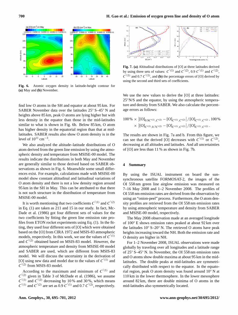
Fig. 7. (a)Altitudinal distributions of [O] at three latitudes derivedby using three sets of values:C

′(1) andC′(2), 0.9C

′(1) andC′(2),

C′(1) and 0.7C

′(1), and(b) the percentage errors of [O] derived byusing the second and third sets of coefficients.

We use the new values to derive the [O] at three latitudes:25◦N/S and the equator, by using the atmospheric tempera-ture and density from SABER. We also calculate the percent-age errors as follows:

100%×∣∣[O]0.9C′(1),C′(2) − [O]C′(1),C′(2)

∣∣/ [O]C′(1),C′(2) ,100%

×∣∣[O]C′(1),0.7C′(2) − [O]C′(1),C′(2)

∣∣/ [O]C′(1),C′(2) .

The results are shown in Fig. 7a and b. From this figure, wecan see that the derived [O] decreases withC

′(1) or C′(2),

decreasing at all altitudes and latitudes. And all uncertaintiesof [O] are less than 11 % as shown in Fig. 7b.

4 Summary

By using the ISUAL instrument on board the sun-synchronous satellite FORMOSAT-2, the images of theOI 558 nm green line airglow emission was measured on7–16 May 2008 and 1–2 November 2008. The profiles ofOI 558 nm emission rates are derived from the observation byusing an “onion-peel” process. Furthermore, the O atom den-sity profiles are retrieved from the OI 558 nm emission ratesby using atmospheric temperature and density from SABERand MSISE-00 model, respectively.

The May 2008 observation made at an averaged longitudeof 100◦ E shows emission rates peaked at about 92 km overthe latitudes 10◦ S–20◦ N. The retrieved O atoms have peakheights increasing toward the NH. Both the emission rate andO density are higher in NH.

For 1–2 November 2008, ISUAL observations were madeglobally by traveling over all longitudes and a latitude rangeof 25◦ S–45◦ N. In November, the OI 558 nm emission ratesand O atoms show double maxima at about 95 km in the mid-latitudes. The double peaks at mid-latitudes are symmetri-cally distributed with respect to the equator. In the equato-rial region, peak O atom density was found around 10◦ N at110 km in the lower thermosphere. In the lower mesospherearound 82 km, there are double minima of O atoms in themid-latitudes also symmetrically located.

Ann. Geophys., 30, 695–701, 2012 www.ann-geophys.net/30/695/2012/

H. Gao et al.: Emission of oxygen green line and density of O atom 701

We also calculate O atom by using SABER OH airglow.The results show similar distribution to that from ISUALgreen line observations.

Acknowledgements.We thank the FORMOSAT-2 andTIMED/SABER science teams for providing the data used inthis study. GH wishes to thank National Science Council forpostdoctor position at NCU. This research is supported through agrant: NSC100-2811-M-008-004. This work is supported by theChinese Academy of Sciences (KZZD-EW-01-2), the NationalScience Foundation of China (41004062, 40921063, 40890165)and the National Important Basic Research Project of China(2011CB811405). The project is also supported by the SpecializedResearch Fund for State Key Laboratories.

Topical Editor C. Jacobi thanks two anonymous referees fortheir help in evaluating this paper.

References

Barth, C. A. and Hildebrandt, A. F.: The 5577 A airglow emissionmechanism, J. Geophys. Res., 66, 985–986, 1961.

Bates, D. R.: Excitation of 557.7 nm OI line in nightglow, Planet.Space Sci., 36, 883–889, 1988.

Capetanakis, F. P., Sondermann, F., Hoser, S., and Stuhl, F.: Tem-perature dependence of the quenching of O(1S) by simple inor-ganic molecules, J. Chem. Phys., 98, 7883–7887, 1993.

Liu, G., Shepherd, G. G., and Roble, R. G.: Seasonal variationsof the nighttime O(1S) and OH airglow emission ratesat mid-to-high latitudes in the context of the large-scale circulation, J. Geo-phys. Res., 113, A06302,doi:10.1029/2007JA012854, 2008a.

Liu, G., Shepherd, G. G., and Tepley, C. A.: Variations of the trop-ical O(1S) nightglow as observed with the Arecibo Observatoryphotometer and WINDII on UARS, J. Atmos. Sol.-Terr. Phys.,70, 1309–1317, 2008b.

Martin, W. C., Fuhr, J. R., Kelleher, D. E., Musgrove, A.,Podobedova, L., Reader, J., Saloman, J. E. B., Sansonetti, C. J.,Wiese, W. L., Mohr, P. J., and Owen, K.: NIST Atomic SpectraDatabase (version 2.0), National Institute of Standards and Tech-nology, Gaithersburg, MD, available at:http://physics.nist.gov/asd, 1999.

McDade, I. C., Murtagh, D. P., Greer, R. G. H., Dickinson, P. H. G.,Witt, G., Stegman, J., Llewellyn, E. J., Thomas, L., and Jenkins,D. B.: ETON 2: Quenching parameters for the proposed precur-sors of O2(b16g+) and O(1S) in the terrestrial nightglow, Planet.Space Sci., 34, 789–800, 1986.

Melo, S. M. L., Takahashi, H., Clemesha, B. R., Batista, P. P., andSimonich, D. M.: Atomic oxygen concentrations from rocket air-glow observations in the equatorial region, J. Atmos. Terr. Phys.,58, 1935–1942, 1996.

Melo, S. M. L., McDade, I. C., and Takahashi, H.: Atomic oxygendensity profiles from ground-based nightglow measurements at23◦ S, J. Geophys. Res., 106, 15377–15384, 2001.

Nakayama, T., Takahashi, K., Matsumi, Y., and Fujiwara, H.: Lab-oratory study of O(1S) formation process in the photolysis of O3and its atmospheric implications, J. Atmos. Chem., 53, 107–122,2006.

Nee, J.-B., Tsai, S.-D., Peng, T.-H., Hsu, R.-R., Chen, A. B.-C.,Zhang, S., Huang, T.-Y., Rajesh, P. K., Liu, J.-Y., Frey, H. U.,and Mende, S. B.: OH Airglow and Equatorial Variations Ob-served by ISUAL Instrument on Board the FORMOSAT-2 Satel-lite, Terr. Atmos. Ocean. Sci., 21, 985–995, 2010.

Reed, E. I. and Chandra, S.: The Global Characteristics of Atmo-spheric Emissions in the Lower Thermosphere and Their Aero-nomic Implications, J. Geophys. Res., 80, 3053–3062, 1975.

Russell, J. M., Mlynczak, M. G., Gordley, L. L., Tansock, J., andEsplin, R.: An overview of the SABER experiment and prelim-inary calibration results, Proc. SPIE Int. Soc. Opt. Eng., 3756,277–288, 1999.

Russell, J. P. and Lowe, R. P.: Atomic oxygen profiles (80–94 km) derived from Wind Imaging Interferometer/Upper At-mospheric Research Satellite measurements of the hydroxyl air-glow: 1. Validation of technique, J. Geophys. Res., 108, 4662,doi:10.1029/2003JD003454, 2003.

Russell, J. P., Lowe, R. P., and Ward, W. E.: Atomic oxygen an-nual and semi-annual variations in the mesopause region for midand equatorial latitudes, J. Atmos. Sol.-Terr. Phys., 66, 451–461,2004.

Shepherd, G. G., Zhang, S., and Wang, X.: Variability in MLT dy-namics and species concentrations as observed by WINDII, EarthPlanets Space, 51, 845–853, 1999.

Skinner, W. R., Yee, J.-H, Hays, P. B., and Burrage, M. D.: Sea-sonal and local time variations in the O(1S) green line, O2 atmo-spheric band, and OH Meinel band emissions as measured by theHigh Resolution Doppler Imager, Adv. Space Res., 21, 835–841,1998.

Smith, A. K., Marsh, D. R., Russell III, J. M., Mlynczak, M. G.,Martin-Torres, F. J., and Kyrola, E.: Satellite observations ofhigh nighttime ozone at the equatorial mesopause, J. Geophys.Res., 113, D17312,doi:10.1029/2008JD010066, 2008.

Smith, A. K., Marsh, D. R., Mlynczak, M. G., and Mast,J. C.: Temporal variations of atomic oxygen in the uppermesosphere from SABER, J. Geophys. Res., 115, D18309,doi:10.1029/2009JD013434, 2010.

Wang, D. Y., Ward, W. E., Solheim, B. H., and Shepherd, G. G.:Longitudinal variations of green line emission rates observed, J.Atmos. Sol.-Terr. Phys., 64, 1273–1286, 2002.

Xu, J., Ji, Q., Wei, Y., and Ma, R.: Comparison between the TIMEDobserved global temperature distribution and the MRLMSISE-00empirical atmospheric model, Chin. J. Space Sci., 26, 177–182,2006 (in Chinese).

Xu, J., Gao, H., Smith, A. K., and Zhu, Y.: Using TIMED/SABERnightglow observations to investigate hydroxyl emission mecha-nisms in the mesopause region, J. Geophys. Res., 117, D02301,doi:10.1029/2011JD016342, 2012.

Yee, J.-H., Crowley, G., Roble, R. G., Skinner, W. R., Burrage,M. D., and Hays, P. B.: Global simulations and observationsof O(1S), O2(16) and OH mesospheric nightglow emissions,J. Geophys. Res., 102, 19949–19968,doi:10.1029/96JA01833,1997.

Zhang, S. P. and Shepherd, G. G.: The influence of the di-urnal tide on the O(1S) and OH emission rates observedby WINDII on UARS, Geophys. Res. Lett., 26, 529–532,doi:10.1029/1999GL900033, 1999.

www.ann-geophys.net/30/695/2012/ Ann. Geophys., 30, 695–701, 2012