The Engineer’s Guide to Motion Compensation

by John Watkinson

HANDBOOK

SERIES

UK £12.50

US $20.00

John Watkinson is an independent author, journalist and consultant inthe broadcast industry with more than 20 years of experience in research

and development.

With a BSc (Hons) in Electronic Engineering and an MSc in Sound andVibration, he has held teaching posts at a senior level with The Digital

Equipment Corporation, Sony Broadcast and Ampex Ltd., before forminghis own consultancy.

Regularly delivering technical papers at conferences including AES,SMPTE, IEE, ITS and Montreux, John Watkinson has also written

numerous publications including “The Art of Digital Video”, “The Art of Digital Audio” and “The Digital Video Tape Recorder.”

The Engineer’s Guide to Motion Compensation

by John Watkinson

Engineering with Vision

INTRODUCTION

There are now quite a few motion compensated products on the market, yet theydo not all work in the same way. The purpose of this document is to clarify theconfusion surrounding motion estimation by explaining clearly how it works, bothin theory and in practice.

Video from different sources may demonstrate widely varying motioncharacteristics. When motion portrayal is poor, all types of motion compensateddevices may appear to perform similarly, despite being widely divergent inapproach. This booklet will explain motion characteristics in such a way as toenable the reader select critical material to reveal tangible performance differencesbetween motion compensation systems.

Motion estimation is a complex subject which is ordinarily discussed inmathematical language. This is not appropriate here, and the new explanationswhich follow will use plain English to make the subject accessible to a wide range ofreaders. In particular a new non-mathematical explanation of the Fourier transformhas been developed which is fundamental to demystifying phase correlation.

CONTENTS

Section 1 – Motion in Television Page 21.1 Motion and the eye1.2 Motion in video systems1.3 Conventional standards conversion1.4 Motion compensated standards conversion1.5 Methods of motion estimation

1.5.1 Block matching1.5.2 Gradient methods1.5.3 Phase correlation

Section 2 – Motion estimation using phase correlation Page 232.1 Phase correlation2.2 Pre-processing2.3 Motion estimation2.4 Image correlation2.5 Vector assignment2.6 Obscured and revealed backgrounds

Section 3 – The Alchemist Page 393.1 Standards conversion3.2 Motion compensation3.3 Interpolation

Section 4 – Further applications Page 494.1 Gazelle - flow motion system4.2 Noise reduction4.3 Oversampling displays4.4 Telecine Transfer

SECTION 1 - MOTION IN TELEVISION

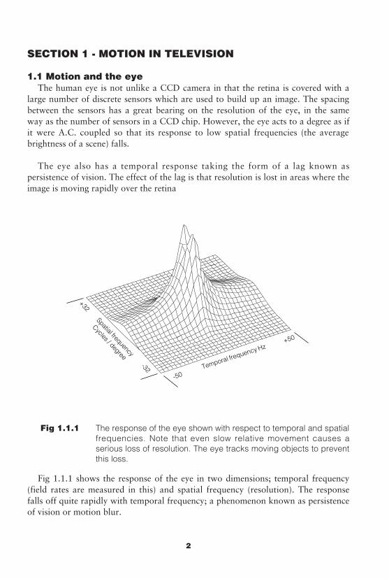
1.1 Motion and the eyeThe human eye is not unlike a CCD camera in that the retina is covered with a

large number of discrete sensors which are used to build up an image. The spacingbetween the sensors has a great bearing on the resolution of the eye, in the sameway as the number of sensors in a CCD chip. However, the eye acts to a degree as ifit were A.C. coupled so that its response to low spatial frequencies (the averagebrightness of a scene) falls.

The eye also has a temporal response taking the form of a lag known aspersistence of vision. The effect of the lag is that resolution is lost in areas where theimage is moving rapidly over the retina

Fig 1.1.1 The response of the eye shown with respect to temporal and spatialfrequencies. Note that even slow relative movement causes aserious loss of resolution. The eye tracks moving objects to preventthis loss.

Fig 1.1.1 shows the response of the eye in two dimensions; temporal frequency(field rates are measured in this) and spatial frequency (resolution). The responsefalls off quite rapidly with temporal frequency; a phenomenon known as persistenceof vision or motion blur.

Temporal frequency Hz

Spatial frequency

Cycles / degree

+32

-50

+50

-32

2

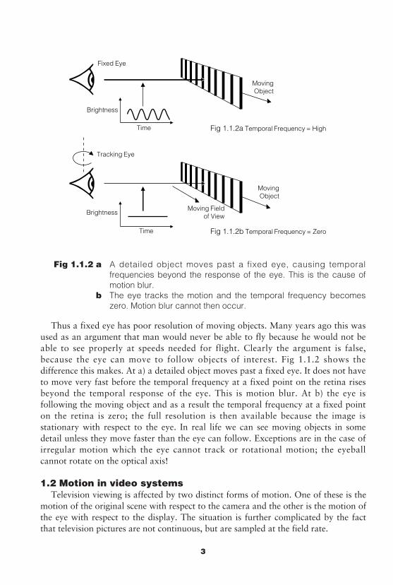
Fig 1.1.2 a A detailed object moves past a fixed eye, causing temporalfrequencies beyond the response of the eye. This is the cause ofmotion blur.

b The eye tracks the motion and the temporal frequency becomeszero. Motion blur cannot then occur.

Thus a fixed eye has poor resolution of moving objects. Many years ago this wasused as an argument that man would never be able to fly because he would not beable to see properly at speeds needed for flight. Clearly the argument is false,because the eye can move to follow objects of interest. Fig 1.1.2 shows thedifference this makes. At a) a detailed object moves past a fixed eye. It does not haveto move very fast before the temporal frequency at a fixed point on the retina risesbeyond the temporal response of the eye. This is motion blur. At b) the eye isfollowing the moving object and as a result the temporal frequency at a fixed pointon the retina is zero; the full resolution is then available because the image isstationary with respect to the eye. In real life we can see moving objects in somedetail unless they move faster than the eye can follow. Exceptions are in the case ofirregular motion which the eye cannot track or rotational motion; the eyeballcannot rotate on the optical axis!

1.2 Motion in video systemsTelevision viewing is affected by two distinct forms of motion. One of these is the

motion of the original scene with respect to the camera and the other is the motion ofthe eye with respect to the display. The situation is further complicated by the factthat television pictures are not continuous, but are sampled at the field rate.

Fixed Eye

Time

Brightness

Moving Fieldof View

Time

Tracking Eye

Brightness

MovingObject

MovingObject

Fig 1.1.2a Temporal Frequency = High

Fig 1.1.2b Temporal Frequency = Zero

3

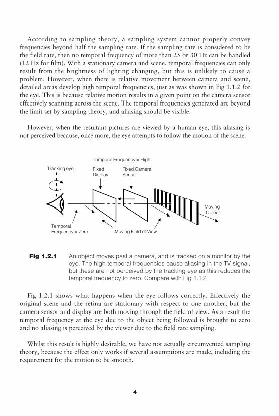
According to sampling theory, a sampling system cannot properly conveyfrequencies beyond half the sampling rate. If the sampling rate is considered to bethe field rate, then no temporal frequency of more than 25 or 30 Hz can be handled(12 Hz for film). With a stationary camera and scene, temporal frequencies can onlyresult from the brightness of lighting changing, but this is unlikely to cause aproblem. However, when there is relative movement between camera and scene,detailed areas develop high temporal frequencies, just as was shown in Fig 1.1.2 forthe eye. This is because relative motion results in a given point on the camera sensoreffectively scanning across the scene. The temporal frequencies generated are beyondthe limit set by sampling theory, and aliasing should be visible.

However, when the resultant pictures are viewed by a human eye, this aliasing isnot perceived because, once more, the eye attempts to follow the motion of the scene.

Fig 1.2.1 An object moves past a camera, and is tracked on a monitor by theeye. The high temporal frequencies cause aliasing in the TV signal,but these are not perceived by the tracking eye as this reduces thetemporal frequency to zero. Compare with Fig 1.1.2

Fig 1.2.1 shows what happens when the eye follows correctly. Effectively theoriginal scene and the retina are stationary with respect to one another, but thecamera sensor and display are both moving through the field of view. As a result thetemporal frequency at the eye due to the object being followed is brought to zeroand no aliasing is perceived by the viewer due to the field rate sampling.

Whilst this result is highly desirable, we have not actually circumvented samplingtheory, because the effect only works if several assumptions are made, including therequirement for the motion to be smooth.

Tracking eye

Temporal Frequency = High

Moving Field of ViewTemporalFrequency = Zero

MovingObject

FixedDisplay

Fixed CameraSensor

4

What is seen is not quite the same as if the scene were being viewed through apiece of moving glass because of the movement of the image relative to the camerasensor and the display. Here, temporal frequencies do exist, and the temporalaperture effect (lag) of both will reduce perceived resolution. This is the reason thatshutters are sometimes fitted to CCD cameras used at sporting events. Themechanically rotating shutter allows light onto the CCD sensor for only part of thefield period thereby reducing the temporal aperture. The result is obvious fromconventional photography in which one naturally uses a short exposure for movingsubjects. The shuttered CCD camera effectively has an exposure control. On theother hand a tube camera displays considerable lag and will not perform as wellunder these circumstances.

It is important to appreciate the effect of camera type and temporal aperture as ithas a great bearing on how to go about assessing or comparing the performance ofmotion compensated standards converters. One of the strengths of motioncompensation is that it improves the resolution of moving objects. Thisimprovement will not be apparent if the source material being used has poor motionqualities in the first place. Using unsuitable (i.e. uncritical) material could result intwo different converters giving the same apparent performance, whereas morecritical material would allow the better convertor to show its paces.

As the greatest problem in standards conversion is the handling of the time axis,it is intended to contrast the time properties of various types of video.

.

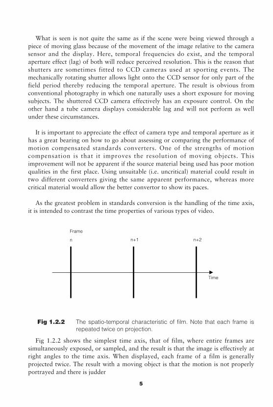
Fig 1.2.2 The spatio-temporal characteristic of film. Note that each frame isrepeated twice on projection.

Fig 1.2.2 shows the simplest time axis, that of film, where entire frames aresimultaneously exposed, or sampled, and the result is that the image is effectively atright angles to the time axis. When displayed, each frame of a film is generallyprojected twice. The result with a moving object is that the motion is not properlyportrayed and there is judder

n

Frame

Time

n+1 n+2

5

.

Fig 1.2.3 The frame repeating results in motion judder as shown here.

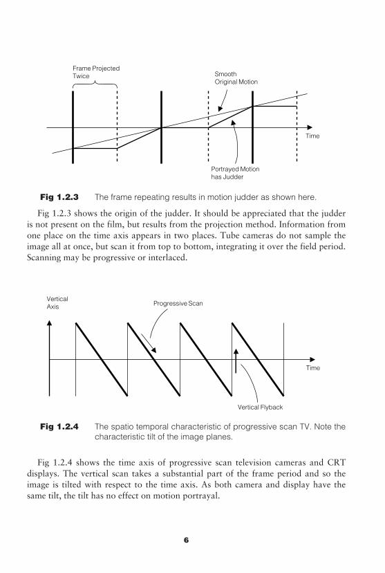
Fig 1.2.3 shows the origin of the judder. It should be appreciated that the judderis not present on the film, but results from the projection method. Information fromone place on the time axis appears in two places. Tube cameras do not sample theimage all at once, but scan it from top to bottom, integrating it over the field period.Scanning may be progressive or interlaced.

Fig 1.2.4 The spatio temporal characteristic of progressive scan TV. Note thecharacteristic tilt of the image planes.

Fig 1.2.4 shows the time axis of progressive scan television cameras and CRTdisplays. The vertical scan takes a substantial part of the frame period and so theimage is tilted with respect to the time axis. As both camera and display have thesame tilt, the tilt has no effect on motion portrayal.

VerticalAxis

Time

Progressive Scan

Vertical Flyback

Frame ProjectedTwice

Time

SmoothOriginal Motion

Portrayed Motionhas Judder

6

.

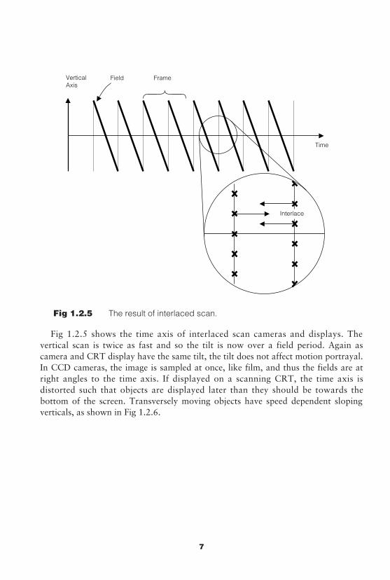
Fig 1.2.5 The result of interlaced scan.

Fig 1.2.5 shows the time axis of interlaced scan cameras and displays. Thevertical scan is twice as fast and so the tilt is now over a field period. Again ascamera and CRT display have the same tilt, the tilt does not affect motion portrayal.In CCD cameras, the image is sampled at once, like film, and thus the fields are atright angles to the time axis. If displayed on a scanning CRT, the time axis isdistorted such that objects are displayed later than they should be towards thebottom of the screen. Transversely moving objects have speed dependent slopingverticals, as shown in Fig 1.2.6.

VerticalAxis

Time

Frame

Interlace

Field

7

.

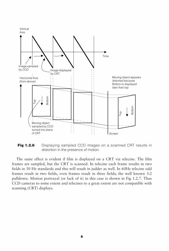
Fig 1.2.6 Displaying sampled CCD images on a scanned CRT results indistortion in the presence of motion.

The same effect is evident if film is displayed on a CRT via telecine. The filmframes are sampled, but the CRT is scanned. In telecine each frame results in twofields in 50 Hz standards and this will result in judder as well. In 60Hz telecine oddframes result in two fields, even frames result in three fields; the well known 3:2pulldown. Motion portrayal (or lack of it) in this case is shown in Fig 1.2.7. ThusCCD cameras to some extent and telecines to a great extent are not compatible withscanning (CRT) displays.

VerticalAxis

Time

Image displayedby CRT

Screen

Horizontal Axis(from above)

Moving objectsampled by CCDturned into planeof CRT

Top

Top

Bot

tom

Bot

tom

Moving object appearsdistorted becauseBottom is displayedlater than top

Image sampledby CCD

8

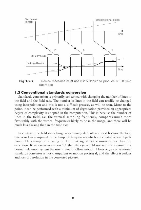
Fig 1.2.7 Telecine machines must use 3:2 pulldown to produce 60 Hz fieldrate video

1.3 Conventional standards conversionStandards conversion is primarily concerned with changing the number of lines in

the field and the field rate. The number of lines in the field can readily be changedusing interpolation and this is not a difficult process, as will be seen. More to thepoint, it can be performed with a minimum of degradation provided an appropriatedegree of complexity is adopted in the computation. This is because the number oflines in the field, i.e. the vertical sampling frequency, compares much morefavourably with the vertical frequencies likely to be in the image, and there will bemuch less aliasing than in the time axis.

In contrast, the field rate change is extremely difficult not least because the fieldrate is so low compared to the temporal frequencies which are created when objectsmove. Thus temporal aliasing in the input signal is the norm rather than theexception. It was seen in section 1.1 that the eye would not see this aliasing in anormal television system because it would follow motion. However, a conventionalstandards convertor is not transparent to motion portrayal, and the effect is judderand loss of resolution in the converted picture.

Film framesat 24Hz

Time

Smooth original motion

Portrayed Motion

Time

60Hz TV fields

2 3 2

9

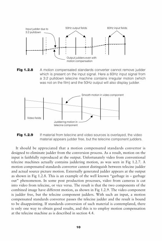
Fig 1.2.8 A motion compensated standards converter cannot remove judderwhich is present on the input signal. Here a 60Hz input signal froma 3:2 pulldown telecine machine contains irregular motion (whichwas not on the film) and the 50Hz output will also display judder.

.

Fig 1.2.9 If material from telecine and video sources is overlayed, the video material appears judder free, but the telecine component judders.

It should be appreciated that a motion compensated standards convertor isdesigned to eliminate judder from the conversion process. As a result, motion on theinput is faithfully reproduced at the output. Unfortunately video from conventionaltelecine machines actually contains juddering motion, as was seen in Fig 1.2.7. Amotion compensated standards convertor cannot distinguish between telecine judderand actual source picture motion. Externally generated judder appears at the outputas shown in Fig 1.2.8. This is an example of the well known “garbage in – garbageout” phenomenon. In some post production processes, video from cameras is cutinto video from telecine, or vice versa. The result is that the two components of thecombined image have different motion, as shown in Fig 1.2.9. The video componentis judder free, but the telecine component judders. With such an input, a motioncompensated standards convertor passes the telecine judder and the result is boundto be disappointing. If standards conversion of such material is contemplated, thereis only one way to obtain good results, and this is to employ motion compensationat the telecine machine as is described in section 4.4.

Video fields

Smooth motion in video component

Juddering motion intelecine component

Input judder due to3:2 pulldown

50Hz output fields

Output judders even withmotion compensation

60Hz input fields

10

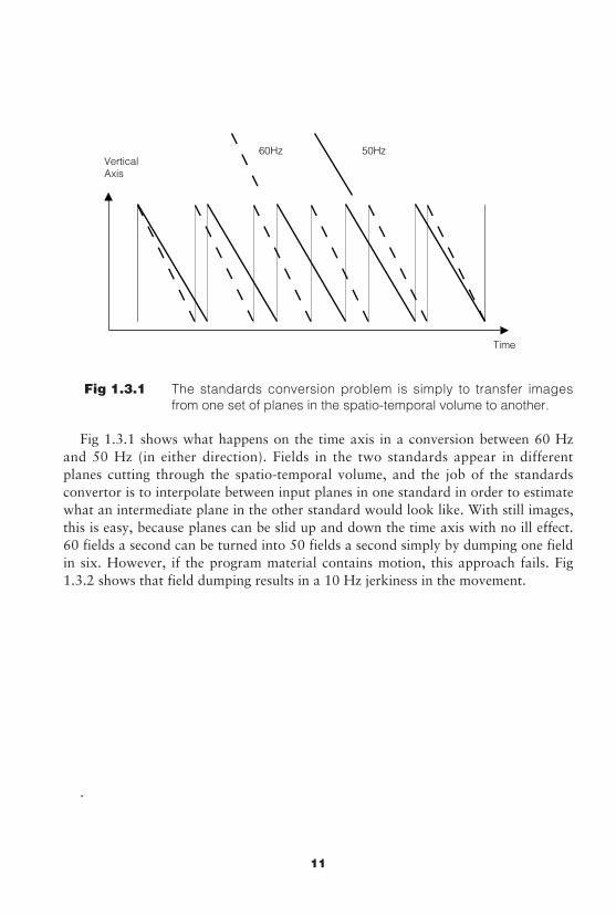
Fig 1.3.1 The standards conversion problem is simply to transfer imagesfrom one set of planes in the spatio-temporal volume to another.

Fig 1.3.1 shows what happens on the time axis in a conversion between 60 Hzand 50 Hz (in either direction). Fields in the two standards appear in differentplanes cutting through the spatio-temporal volume, and the job of the standardsconvertor is to interpolate between input planes in one standard in order to estimatewhat an intermediate plane in the other standard would look like. With still images,this is easy, because planes can be slid up and down the time axis with no ill effect.60 fields a second can be turned into 50 fields a second simply by dumping one fieldin six. However, if the program material contains motion, this approach fails. Fig1.3.2 shows that field dumping results in a 10 Hz jerkiness in the movement.

.

VerticalAxis

Time

60Hz 50Hz

11

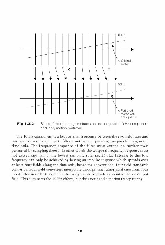
Fig 1.3.2 Simple field dumping produces an unacceptable 10 Hz componentand jerky motion portrayal.

The 10 Hz component is a beat or alias frequency between the two field rates andpractical converters attempt to filter it out by incorporating low pass filtering in thetime axis. The frequency response of the filter must extend no further thanpermitted by sampling theory. In other words the temporal frequency response mustnot exceed one half of the lowest sampling rate, i.e. 25 Hz. Filtering to this lowfrequency can only be achieved by having an impulse response which spreads overat least four fields along the time axis, hence the conventional four-field standardsconvertor. Four field converters interpolate through time, using pixel data from fourinput fields in order to compute the likely values of pixels in an intermediate outputfield. This eliminates the 10 Hz effects, but does not handle motion transparently.

Originalmotion

50Hz

60Hz

Portrayedmotion with10Hz judder

12

.

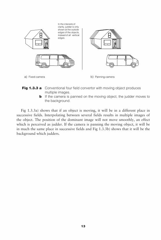
Fig 1.3.3 a Conventional four field convertor with moving object produces multiple images.

b If the camera is panned on the moving object, the judder moves tothe background.

Fig 1.3.3a) shows that if an object is moving, it will be in a different place insuccessive fields. Interpolating between several fields results in multiple images ofthe object. The position of the dominant image will not move smoothly, an effectwhich is perceived as judder. If the camera is panning the moving object, it will bein much the same place in successive fields and Fig 1.3.3b) shows that it will be thebackground which judders.

a) Fixed camera b) Panning camera

In the interests ofclarity, judder is onlyshown at the outsideedges of the objects,instead of all verticaledges.

13

.

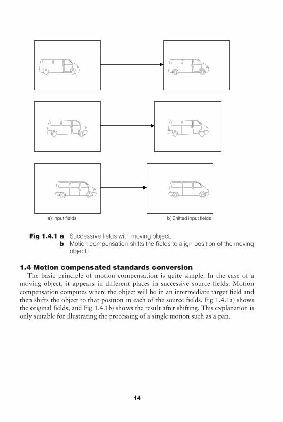
Fig 1.4.1 a Successive fields with moving object.b Motion compensation shifts the fields to align position of the moving

object.

1.4 Motion compensated standards conversionThe basic principle of motion compensation is quite simple. In the case of a

moving object, it appears in different places in successive source fields. Motioncompensation computes where the object will be in an intermediate target field andthen shifts the object to that position in each of the source fields. Fig 1.4.1a) showsthe original fields, and Fig 1.4.1b) shows the result after shifting. This explanation isonly suitable for illustrating the processing of a single motion such as a pan.

a) Input fields b) Shifted input fields

14

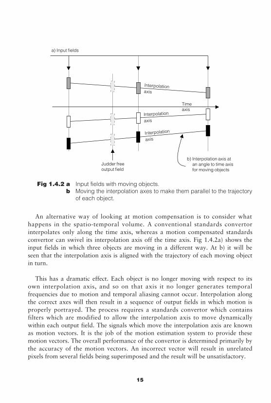
Fig 1.4.2 a Input fields with moving objects.b Moving the interpolation axes to make them parallel to the trajectory

of each object.

An alternative way of looking at motion compensation is to consider whathappens in the spatio-temporal volume. A conventional standards convertorinterpolates only along the time axis, whereas a motion compensated standardsconvertor can swivel its interpolation axis off the time axis. Fig 1.4.2a) shows theinput fields in which three objects are moving in a different way. At b) it will beseen that the interpolation axis is aligned with the trajectory of each moving objectin turn.

This has a dramatic effect. Each object is no longer moving with respect to itsown interpolation axis, and so on that axis it no longer generates temporalfrequencies due to motion and temporal aliasing cannot occur. Interpolation alongthe correct axes will then result in a sequence of output fields in which motion isproperly portrayed. The process requires a standards convertor which containsfilters which are modified to allow the interpolation axis to move dynamicallywithin each output field. The signals which move the interpolation axis are knownas motion vectors. It is the job of the motion estimation system to provide thesemotion vectors. The overall performance of the convertor is determined primarily bythe accuracy of the motion vectors. An incorrect vector will result in unrelatedpixels from several fields being superimposed and the result will be unsatisfactory.

Timeaxis

a) Input fields

Interpolationaxis

Interpolation

axis

Interpolation

axis

Judder freeoutput field

b) Interpolation axis atan angle to time axisfor moving objects

15

.

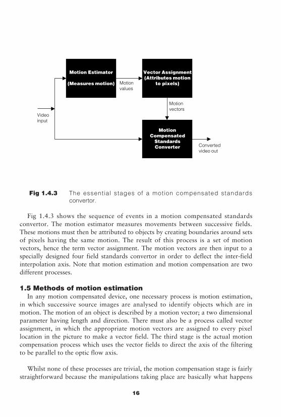
Fig 1.4.3 The essential stages of a motion compensated standardsconvertor.

Fig 1.4.3 shows the sequence of events in a motion compensated standardsconvertor. The motion estimator measures movements between successive fields.These motions must then be attributed to objects by creating boundaries around setsof pixels having the same motion. The result of this process is a set of motionvectors, hence the term vector assignment. The motion vectors are then input to aspecially designed four field standards convertor in order to deflect the inter-fieldinterpolation axis. Note that motion estimation and motion compensation are twodifferent processes.

1.5 Methods of motion estimationIn any motion compensated device, one necessary process is motion estimation,

in which successive source images are analysed to identify objects which are inmotion. The motion of an object is described by a motion vector; a two dimensionalparameter having length and direction. There must also be a process called vectorassignment, in which the appropriate motion vectors are assigned to every pixellocation in the picture to make a vector field. The third stage is the actual motioncompensation process which uses the vector fields to direct the axis of the filteringto be parallel to the optic flow axis.

Whilst none of these processes are trivial, the motion compensation stage is fairlystraightforward because the manipulations taking place are basically what happens

Convertedvideo out

Motion Estimator

(Measures motion)

Motionvectors

Vector Assignment(Attributes motion

to pixels)

MotionCompensated

StandardsConverter

Videoinput

Motionvalues

16

in a DVE. In motion estimation it is not the details of the problem which causedifficulty, but the magnitude. All of the available techniques need a fair amount ofprocessing power. Here the criterion is to select an algorithm which gives the bestefficiency at the desired performance level. In practice the most difficult section of amachine to engineer is the logic which interprets the output of the motion estimator.Another area in which care is needed is in the pre-processing which is necessary toallow motion estimation to take place between fields. The use of interlace meansthat one field cannot be compared directly with the next because the available pixelsare in different places in the image.

As television signals are effectively undersampled in the time axis, it is impossibleto make a motion estimator which always works. Difficult inputs having periodicstructures or highly irregular motion may result in incorrect estimation. Since anymotion estimation system will fail, it is important to consider how such a failure ishandled. It is better to have a graceful transition to conventional conversion than aspectacular failure. Motion estimation techniques can also be compared on theallowable speed range and precision. Standards conversion of sporting events willrequire a large motion range, whereas correction of film weave will require a rangeof a couple of pixels at worst, but will need higher sub-pixel accuracy. A slow-motion system needs both. Finally estimators can be compared on the number ofdifferent motions which can be handled at once. There are a number of estimationtechniques which can be used, and these are compared below. It is dangerous togeneralise about actual products as a result of these descriptions. The terminology isnot always used consistently, techniques are seldom used alone or in a pure form,and the quality of the vector assignment process is just as important, perhaps moreimportant, in determining performance.

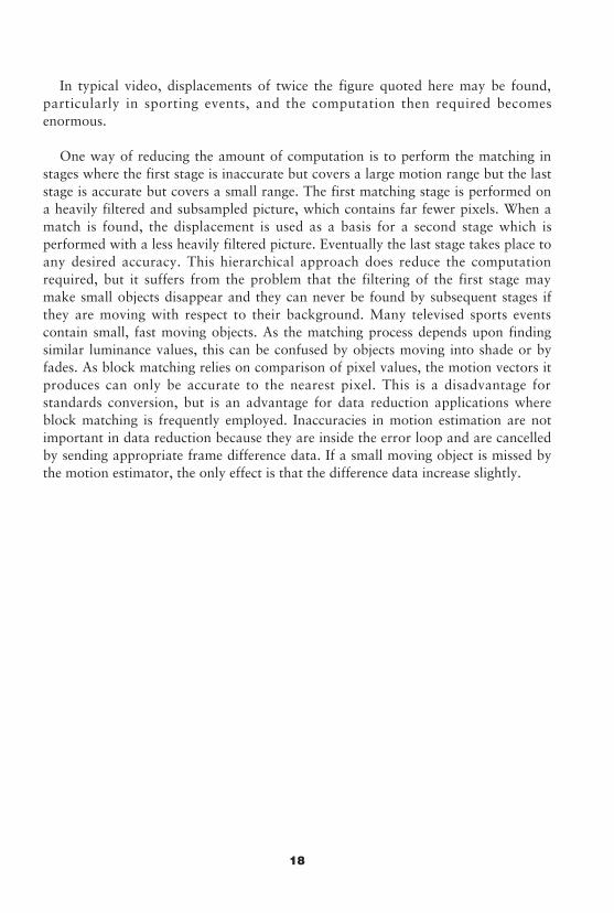
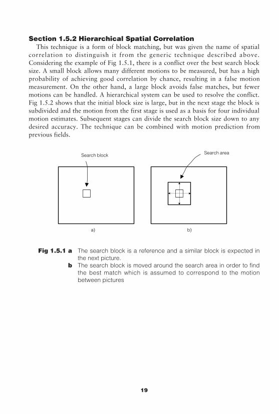
1.5.1 Block matchingFig 1.5.1 shows a block of pixels in an image. This block is compared, a pixel at

a time, with a similarly sized block b) in the same place in the next image. If there isno motion between fields, there will be high correlation between the pixel values.However, in the case of motion, the same, or similar pixel values will be elsewhereand it will be necessary to search for them by moving the search block to allpossible locations in the search area. The location which gives the best correlation isassumed to be the new location of a moving object.

Whilst simple in concept, block matching requires an enormous amount ofcomputation because every possible motion must be tested over the assumed range.Thus if the object is assumed to have moved over a sixteen pixel range, then it willbe necessary to test 16 different horizontal displacements in each of sixteen verticalpositions; in excess of 65,000 positions. At each position every pixel in the blockmust be compared with every pixel in the second picture.

17

In typical video, displacements of twice the figure quoted here may be found,particularly in sporting events, and the computation then required becomesenormous.

One way of reducing the amount of computation is to perform the matching instages where the first stage is inaccurate but covers a large motion range but the laststage is accurate but covers a small range. The first matching stage is performed ona heavily filtered and subsampled picture, which contains far fewer pixels. When amatch is found, the displacement is used as a basis for a second stage which isperformed with a less heavily filtered picture. Eventually the last stage takes place toany desired accuracy. This hierarchical approach does reduce the computationrequired, but it suffers from the problem that the filtering of the first stage maymake small objects disappear and they can never be found by subsequent stages ifthey are moving with respect to their background. Many televised sports eventscontain small, fast moving objects. As the matching process depends upon findingsimilar luminance values, this can be confused by objects moving into shade or byfades. As block matching relies on comparison of pixel values, the motion vectors itproduces can only be accurate to the nearest pixel. This is a disadvantage forstandards conversion, but is an advantage for data reduction applications whereblock matching is frequently employed. Inaccuracies in motion estimation are notimportant in data reduction because they are inside the error loop and are cancelledby sending appropriate frame difference data. If a small moving object is missed bythe motion estimator, the only effect is that the difference data increase slightly.

18

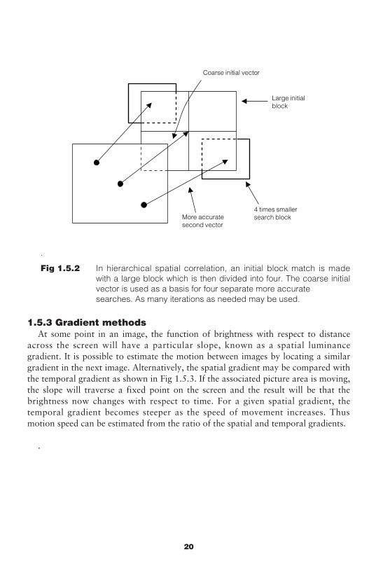
Section 1.5.2 Hierarchical Spatial CorrelationThis technique is a form of block matching, but was given the name of spatial

correlation to distinguish it from the generic technique described above.Considering the example of Fig 1.5.1, there is a conflict over the best search blocksize. A small block allows many different motions to be measured, but has a highprobability of achieving good correlation by chance, resulting in a false motionmeasurement. On the other hand, a large block avoids false matches, but fewermotions can be handled. A hierarchical system can be used to resolve the conflict.Fig 1.5.2 shows that the initial block size is large, but in the next stage the block issubdivided and the motion from the first stage is used as a basis for four individualmotion estimates. Subsequent stages can divide the search block size down to anydesired accuracy. The technique can be combined with motion prediction fromprevious fields.

Fig 1.5.1 a The search block is a reference and a similar block is expected inthe next picture.

b The search block is moved around the search area in order to findthe best match which is assumed to correspond to the motionbetween pictures

Search areaSearch block

a) b)

19

.

Fig 1.5.2 In hierarchical spatial correlation, an initial block match is madewith a large block which is then divided into four. The coarse initialvector is used as a basis for four separate more accurate searches. As many iterations as needed may be used.

1.5.3 Gradient methodsAt some point in an image, the function of brightness with respect to distance

across the screen will have a particular slope, known as a spatial luminancegradient. It is possible to estimate the motion between images by locating a similargradient in the next image. Alternatively, the spatial gradient may be compared withthe temporal gradient as shown in Fig 1.5.3. If the associated picture area is moving,the slope will traverse a fixed point on the screen and the result will be that thebrightness now changes with respect to time. For a given spatial gradient, thetemporal gradient becomes steeper as the speed of movement increases. Thusmotion speed can be estimated from the ratio of the spatial and temporal gradients.

.

Large initialblock

Coarse initial vector

4 times smallersearch blockMore accurate

second vector

20

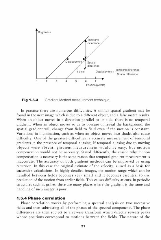
Fig 1.5.3 Gradient Method measurement technique

In practice there are numerous difficulties. A similar spatial gradient may befound in the next image which is due to a different object, and a false match results.When an object moves in a direction parallel to its side, there is no temporalgradient. When an object moves so as to obscure or reveal the background, thespatial gradient will change from field to field even if the motion is constant.Variations in illumination, such as when an object moves into shade, also causedifficulty. One of the greatest difficulties is accurate measurement of temporalgradients in the presence of temporal aliasing. If temporal aliasing due to movingobjects were absent, gradient measurement would be easy, but motioncompensation would not be necessary. Stated differently, the reason why motioncompensation is necessary is the same reason that temporal gradient measurement isinaccurate. The accuracy of both gradient methods can be improved by usingrecursion. In this case the original estimate of the velocity is used as a basis forsuccessive calculations. In highly detailed images, the motion range which can behandled between fields becomes very small and it becomes essential to useprediction of the motion from earlier fields. This causes difficulty at cuts. In periodicstructures such as grilles, there are many places where the gradient is the same andhandling of such images is poor.

1.5.4 Phase correlationPhase correlation works by performing a spectral analysis on two successive

fields and then subtracting all of the phases of the spectral components. The phasedifferences are then subject to a reverse transform which directly reveals peakswhose positions correspond to motions between the fields. The nature of the

Displacement

Brightness

1 pixel

Temporaldifference

Spatialdifference

1 2 3 4 5 6 7Position (pixels)

Displacement =Temporal difference

Spatial difference

21

transform domain means that if the distance and direction of the motion ismeasured accurately, the area of the screen in which it took place is not. Thus inpractical systems the phase correlation stage is followed by a matching stage notdissimilar to the block matching process. However, the matching process is steeredby the motions from the phase correlation, and so there is no need to attempt tomatch at all possible motions. By attempting matching on measured motion only theoverall process is made much more efficient.

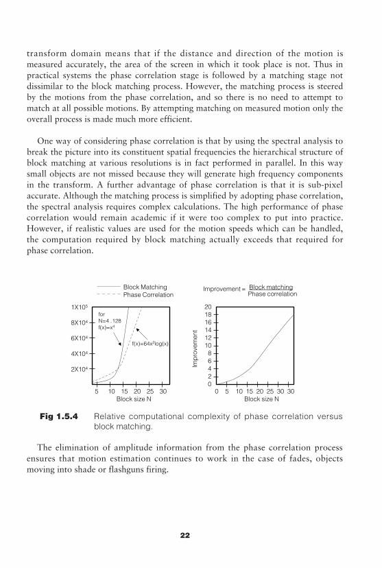
One way of considering phase correlation is that by using the spectral analysis tobreak the picture into its constituent spatial frequencies the hierarchical structure ofblock matching at various resolutions is in fact performed in parallel. In this waysmall objects are not missed because they will generate high frequency componentsin the transform. A further advantage of phase correlation is that it is sub-pixelaccurate. Although the matching process is simplified by adopting phase correlation,the spectral analysis requires complex calculations. The high performance of phasecorrelation would remain academic if it were too complex to put into practice.However, if realistic values are used for the motion speeds which can be handled,the computation required by block matching actually exceeds that required forphase correlation.

Fig 1.5.4 Relative computational complexity of phase correlation versusblock matching.

The elimination of amplitude information from the phase correlation processensures that motion estimation continues to work in the case of fades, objectsmoving into shade or flashguns firing.

5 10 15 20 25 30Block size N

Improvement = Block matchingPhase correlation

0 5 10 15 20 25 30 30Block size N

20181614121086420

1X105

8X104

6X104

4X104

2X104

Block MatchingPhase Correlation

f(x)=64x2log(x)

forN=4..128f(x)=x4

Imp

rove

men

t

22

Section 2 - MOTION ESTIMATION USING PHASE

CORRELATION

Based on the conclusions of the previous section, Phase Correlation has a greatdeal to offer, but is a complex process, and warrants a detailed explanation.

The use of motion compensation enhances standards conversion by movingpicture areas across the screen to properly portray motion in a different fieldstructure (see fig 1.4.1). Motion compensation is the process of modifying theoperation of a nearly conventional standards convertor. The motion compensationitself is controlled by parameters known as motion vectors which are produced bythe motion estimation unit. It should be stressed that phase correlation is just onestep, albeit a critical one, in the motion estimation process.

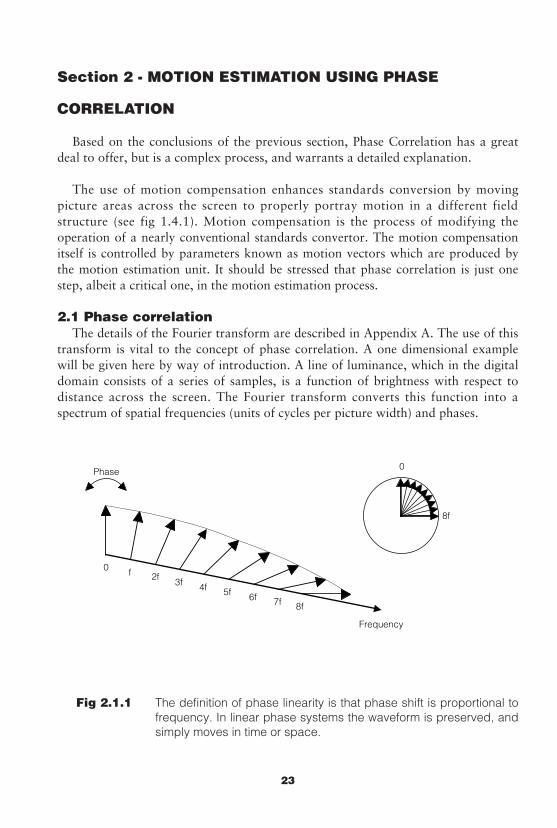
2.1 Phase correlationThe details of the Fourier transform are described in Appendix A. The use of this

transform is vital to the concept of phase correlation. A one dimensional examplewill be given here by way of introduction. A line of luminance, which in the digitaldomain consists of a series of samples, is a function of brightness with respect todistance across the screen. The Fourier transform converts this function into aspectrum of spatial frequencies (units of cycles per picture width) and phases.

.

Fig 2.1.1 The definition of phase linearity is that phase shift is proportional tofrequency. In linear phase systems the waveform is preserved, andsimply moves in time or space.

Frequency

Phase 0

8f

0 f 2f3f

5f 6f 7f 8f

4f

23

All television signals must be handled in linear-phase systems. A linear phasesystem is one in which the delay experienced is the same for all frequencies. If videosignals pass through a device which does not exhibit linear phase, the variousfrequency components of edges become displaced across the screen. Fig 2.1.1 showswhat phase linearity means. If the left hand end of the frequency axis (0) isconsidered to be firmly anchored, but the right hand end can be rotated to representa change of position across the screen, it will be seen that as the axis twists evenlythe result is phase shift proportional to frequency. A system having thischaracteristic is said to have linear phase.

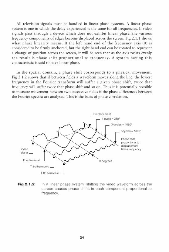
In the spatial domain, a phase shift corresponds to a physical movement.Fig 2.1.2 shows that if between fields a waveform moves along the line, the lowestfrequency in the Fourier transform will suffer a given phase shift, twice thatfrequency will suffer twice that phase shift and so on. Thus it is potentially possibleto measure movement between two successive fields if the phase differences betweenthe Fourier spectra are analysed. This is the basis of phase correlation.

.

Fig 2.1.2 In a linear phase system, shifting the video waveform across thescreen causes phase shifts in each component proportional tofrequency.

0 degrees

Videosignal

Displacement

Fundamental

Fifth harmonic

Third harmonic

1 cycle = 360°

3 cycles = 1080°

5cycles = 1800°

Phase shiftproportional todisplacementtimes frequency

24

.

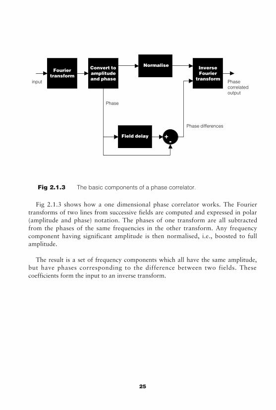
Fig 2.1.3 The basic components of a phase correlator.

Fig 2.1.3 shows how a one dimensional phase correlator works. The Fouriertransforms of two lines from successive fields are computed and expressed in polar(amplitude and phase) notation. The phases of one transform are all subtractedfrom the phases of the same frequencies in the other transform. Any frequencycomponent having significant amplitude is then normalised, i.e., boosted to fullamplitude.

The result is a set of frequency components which all have the same amplitude,but have phases corresponding to the difference between two fields. Thesecoefficients form the input to an inverse transform.

Phasecorrelatedoutput

Fouriertransform

Normalise InverseFourier

transforminput

Convert toamplitudeand phase

Field delay

Phase differences

Phase

25

.

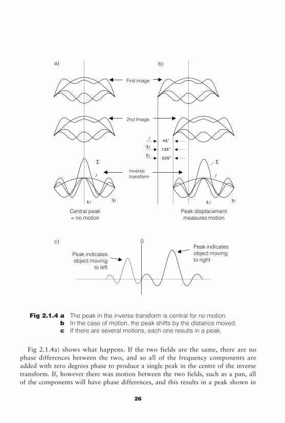
Fig 2.1.4 a The peak in the inverse transform is central for no motion. b In the case of motion, the peak shifts by the distance moved. c If there are several motions, each one results in a peak.

Fig 2.1.4a) shows what happens. If the two fields are the same, there are nophase differences between the two, and so all of the frequency components areadded with zero degrees phase to produce a single peak in the centre of the inversetransform. If, however there was motion between the two fields, such as a pan, allof the components will have phase differences, and this results in a peak shown in

First image

Inversetransform

2nd Image

Central peak= no motion

Peak displacementmeasures motion

a) b)

c)Peak indicatesobject movingto right

Peak indicatesobject moving

to left

0

26

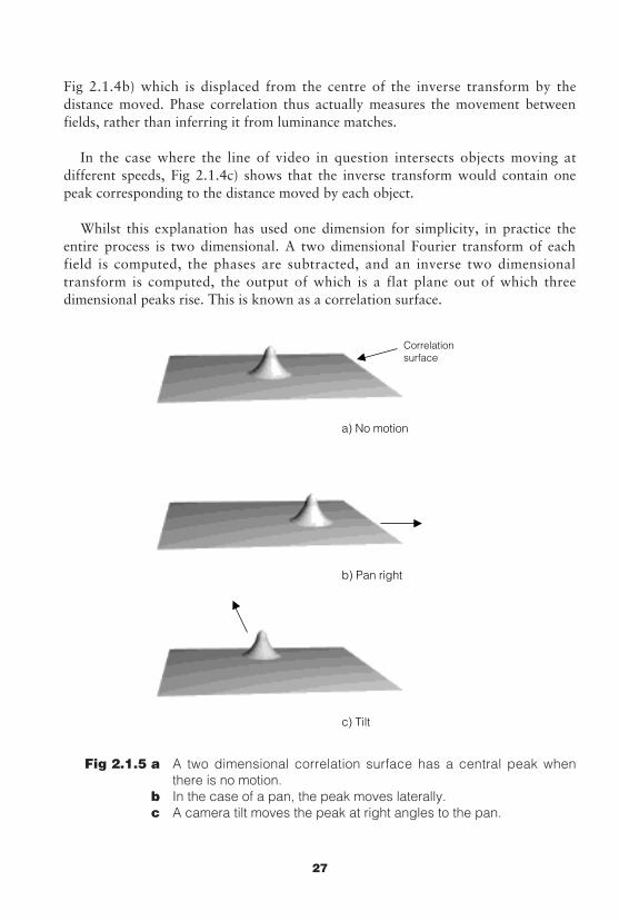
Fig 2.1.4b) which is displaced from the centre of the inverse transform by thedistance moved. Phase correlation thus actually measures the movement betweenfields, rather than inferring it from luminance matches.

In the case where the line of video in question intersects objects moving atdifferent speeds, Fig 2.1.4c) shows that the inverse transform would contain onepeak corresponding to the distance moved by each object.

Whilst this explanation has used one dimension for simplicity, in practice theentire process is two dimensional. A two dimensional Fourier transform of eachfield is computed, the phases are subtracted, and an inverse two dimensionaltransform is computed, the output of which is a flat plane out of which threedimensional peaks rise. This is known as a correlation surface.

Fig 2.1.5 a A two dimensional correlation surface has a central peak whenthere is no motion.

b In the case of a pan, the peak moves laterally.c A camera tilt moves the peak at right angles to the pan.

a) No motion

b) Pan right

c) Tilt

Correlationsurface

27

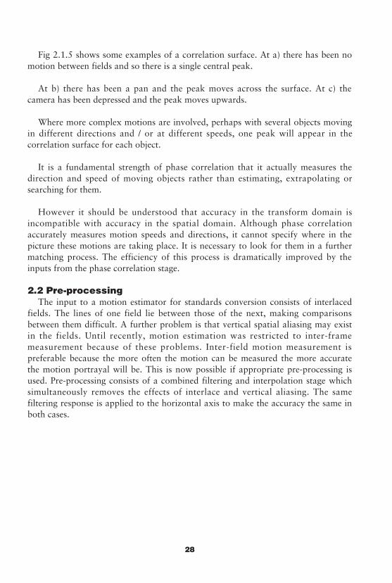
Fig 2.1.5 shows some examples of a correlation surface. At a) there has been nomotion between fields and so there is a single central peak.

At b) there has been a pan and the peak moves across the surface. At c) thecamera has been depressed and the peak moves upwards.

Where more complex motions are involved, perhaps with several objects movingin different directions and / or at different speeds, one peak will appear in thecorrelation surface for each object.

It is a fundamental strength of phase correlation that it actually measures thedirection and speed of moving objects rather than estimating, extrapolating orsearching for them.

However it should be understood that accuracy in the transform domain isincompatible with accuracy in the spatial domain. Although phase correlationaccurately measures motion speeds and directions, it cannot specify where in thepicture these motions are taking place. It is necessary to look for them in a furthermatching process. The efficiency of this process is dramatically improved by theinputs from the phase correlation stage.

2.2 Pre-processingThe input to a motion estimator for standards conversion consists of interlaced

fields. The lines of one field lie between those of the next, making comparisonsbetween them difficult. A further problem is that vertical spatial aliasing may existin the fields. Until recently, motion estimation was restricted to inter-framemeasurement because of these problems. Inter-field motion measurement ispreferable because the more often the motion can be measured the more accuratethe motion portrayal will be. This is now possible if appropriate pre-processing isused. Pre-processing consists of a combined filtering and interpolation stage whichsimultaneously removes the effects of interlace and vertical aliasing. The samefiltering response is applied to the horizontal axis to make the accuracy the same inboth cases.

28

.

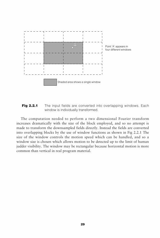
Fig 2.2.1 The input fields are converted into overlapping windows. Eachwindow is individually transformed.

The computation needed to perform a two dimensional Fourier transformincreases dramatically with the size of the block employed, and so no attempt ismade to transform the downsampled fields directly. Instead the fields are convertedinto overlapping blocks by the use of window functions as shown in Fig 2.2.1 Thesize of the window controls the motion speed which can be handled, and so awindow size is chosen which allows motion to be detected up to the limit of humanjudder visibility. The window may be rectangular because horizontal motion is morecommon than vertical in real program material.

Point ’A’ appears infour different windows

Shaded area shows a single window

29

2.3 Motion estimation

Fig 2.3.1 The block diagram of a phase correlated motion estimator

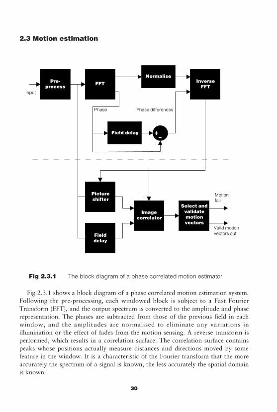
Fig 2.3.1 shows a block diagram of a phase correlated motion estimation system.Following the pre-processing, each windowed block is subject to a Fast FourierTransform (FFT), and the output spectrum is converted to the amplitude and phaserepresentation. The phases are subtracted from those of the previous field in eachwindow, and the amplitudes are normalised to eliminate any variations inillumination or the effect of fades from the motion sensing. A reverse transform isperformed, which results in a correlation surface. The correlation surface containspeaks whose positions actually measure distances and directions moved by somefeature in the window. It is a characteristic of the Fourier transform that the moreaccurately the spectrum of a signal is known, the less accurately the spatial domainis known.

Motionfail

Pre-process

NormaliseInverse

FFTinput

FFT

Pictureshifter

Phase differencesPhase

Fielddelay

Imagecorrelator

Select andvalidatemotionvectors

Valid motionvectors out

Field delay

30

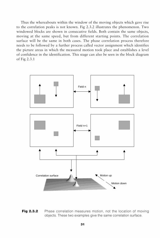
Thus the whereabouts within the window of the moving objects which gave riseto the correlation peaks is not known. Fig 2.3.2 illustrates the phenomenon. Twowindowed blocks are shown in consecutive fields. Both contain the same objects,moving at the same speed, but from different starting points. The correlationsurface will be the same in both cases. The phase correlation process thereforeneeds to be followed by a further process called vector assignment which identifiesthe picture areas in which the measured motion took place and establishes a levelof confidence in the identification. This stage can also be seen in the block diagramof Fig 2.3.1

.

Fig 2.3.2 Phase correlation measures motion, not the location of movingobjects. These two examples give the same correlation surface.

Field n

Motion up

Field n+1

Motion down

Correlation surface

31

To employ the terminology of motion estimation, the phase correlation processproduces candidate vectors, and a process called image correlation assigns thevectors to specific areas of the picture. In many ways the vector assignment processis more difficult than the phase correlation process as the latter is a fixedcomputation whereas the vector assignment has to respond to infinitely varyingpicture conditions.

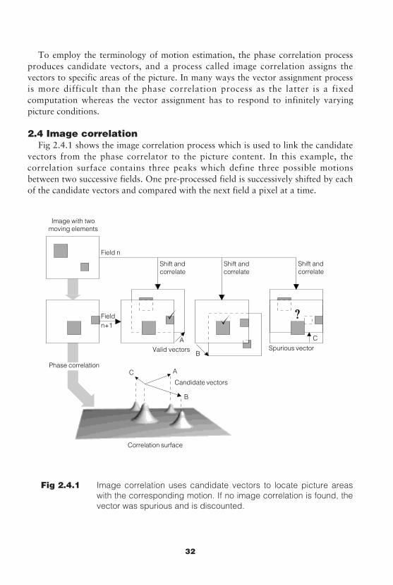
2.4 Image correlationFig 2.4.1 shows the image correlation process which is used to link the candidate

vectors from the phase correlator to the picture content. In this example, thecorrelation surface contains three peaks which define three possible motionsbetween two successive fields. One pre-processed field is successively shifted by eachof the candidate vectors and compared with the next field a pixel at a time.

.

Fig 2.4.1 Image correlation uses candidate vectors to locate picture areaswith the corresponding motion. If no image correlation is found, thevector was spurious and is discounted.

Field n

Candidate vectors

AC

Valid vectorsA

BSpurious vector

C

Fieldn+1

Shift andcorrelate

Shift andcorrelate

Shift andcorrelate

Correlation surface

Phase correlation

Image with twomoving elements

B

32

Similarities or correlations between pixel values indicate that an area with themeasured motion has been found. This happens for two of the candidate vectors,and these vectors are then assigned to those areas. However, shifting by the thirdvector does not result in a meaningful correlation. This is taken to mean that it wasa spurious vector; one which was produced in error because of difficult programmaterial. The ability to eliminate spurious vectors and establish confidence levels inthose which remain is essential to artifact-free conversion.

Image correlation is a form of matching because it is looking for similarluminance values in successive fields. However, image correlation is performed afterthe motion estimation when the motion is known, whereas block matching is usedto estimate the motion. Thus the number of correlations which a block matchermust perform is very high compared to those needed by an image correlator. Theprobability of error is therefore much smaller. The image correlator is not lookingfor motion because this is already known. Instead it is looking for the outline ofobjects having that known motion.

33

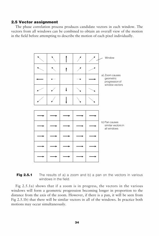
2.5 Vector assignmentThe phase correlation process produces candidate vectors in each window. The

vectors from all windows can be combined to obtain an overall view of the motionin the field before attempting to describe the motion of each pixel individually.

Fig 2.5.1 The results of a) a zoom and b) a pan on the vectors in variouswindows in the field.

Fig 2.5.1a) shows that if a zoom is in progress, the vectors in the variouswindows will form a geometric progression becoming longer in proportion to thedistance from the axis of the zoom. However, if there is a pan, it will be seen fromFig 2.5.1b) that there will be similar vectors in all of the windows. In practice bothmotions may occur simultaneously.

Window

a) Zoom causesgeometricprogression ofwindow vectors

b) Pan causessimilar vectors inall windows

34

An estimate will be made of the speed of a field-wide zoom, or of the speed ofpicture areas which contain receding or advancing motions which give a zoom-likeeffect. If the effect of zooming is removed from each window by shifting the peaksby the local zoom magnitude, but in the opposite direction, the position of the peakswill reveal any component due to panning. This can be found by summing all of thewindows to create a histogram. Panning results in a dominant peak in the histogramwhere all windows contain peaks in a similar place which reinforce.

Each window is then processed in turn. Where only a small part of an objectoverlaps into a window, it will result in a small peak in the correlation surfacewhich might be missed. The windows are deliberately overlapped so that a givenpixel may appear in four windows. Thus a moving object will appear in more thanone window. If the majority of an object lies within one window, a large peak willbe produced from the motion in that window. The resulting vector will be added tothe candidate vector list of all adjacent windows. When the vector assignment isperformed, image correlations will result if a small overlap occurred, and the vectorwill be validated. If there was no overlap, the vector will be rejected.

The peaks in each window reflect the degree of correlation between the two fieldsfor different offsets in two dimensions. The volume of the peak corresponds to theamount of the area of the window (i.e. the number of pixels) having that motion.Thus the largest peak should be selected first.

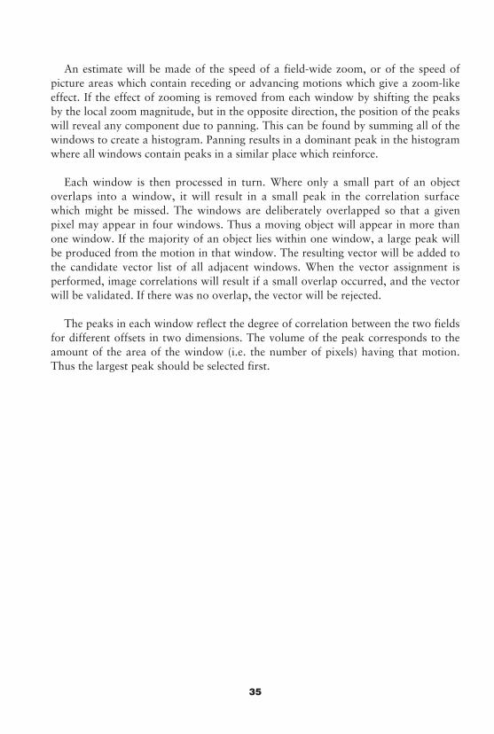
35

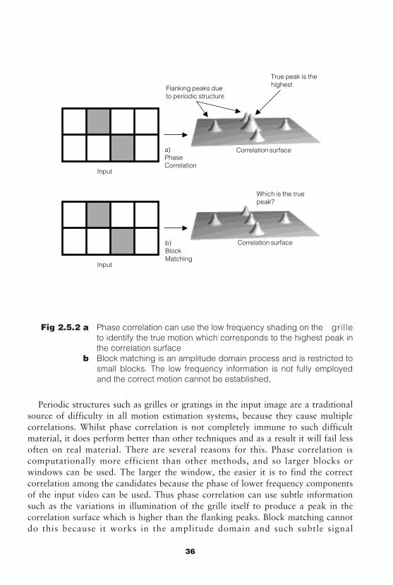
Fig 2.5.2 a Phase correlation can use the low frequency shading on the grilleto identify the true motion which corresponds to the highest peak inthe correlation surface

b Block matching is an amplitude domain process and is restricted tosmall blocks. The low frequency information is not fully employedand the correct motion cannot be established,

Periodic structures such as grilles or gratings in the input image are a traditionalsource of difficulty in all motion estimation systems, because they cause multiplecorrelations. Whilst phase correlation is not completely immune to such difficultmaterial, it does perform better than other techniques and as a result it will fail lessoften on real material. There are several reasons for this. Phase correlation iscomputationally more efficient than other methods, and so larger blocks orwindows can be used. The larger the window, the easier it is to find the correctcorrelation among the candidates because the phase of lower frequency componentsof the input video can be used. Thus phase correlation can use subtle informationsuch as the variations in illumination of the grille itself to produce a peak in thecorrelation surface which is higher than the flanking peaks. Block matching cannotdo this because it works in the amplitude domain and such subtle signal

Input

b)BlockMatching

a)PhaseCorrelation

Input

Flanking peaks dueto periodic structure

Which is the truepeak?

True peak is thehighest

Correlation surface

Correlation surface

36

components result in noise which reduces the correct correlation and the false onesalike. Fig 2.5.2a) shows the correlation surface of a phase correlated motionestimator when a periodic structure is input. The central peak is larger than theflanking peaks because correlation of all image frequencies takes place there. Inblock matching, shown at b) the correlation peaks are periodic but the amplitudesare not a reliable indication of the correct peak. A further way in which multiplecorrelations may be handled is to compare the position of the peaks in each windowwith those estimated by the pan/zoom process. The true peak due to motion will besimilar; the sub peaks due to image periodicity will not be and can be rejected.

Correlations with candidate vectors are then performed. The image in one field isshifted in an interpolator by the amount specified by a candidate vector and thedegree of correlation is measured. Note that this interpolation is to sub-pixelaccuracy because phase correlation can accurately measure sub-pixel motion. Highcorrelation results in vector assignment, low correlation results in the vector beingrejected as unreliable.

If all of the peaks are evaluated in this way, then most of the time validassignments will be made for which there is acceptable confidence from thecorrelator. Should it not be possible to obtain any correlation with confidence in awindow, then the pan/zoom values will be inserted so that that window moves in asimilar way to the overall field motion.

2.6 Obscured and revealed backgroundsWhen objects move, they obscure their background at the leading edge and reveal

it at the trailing edge. As a motion compensated standards convertor will besynthesising moving objects in positions which are intermediate to those in the inputfields, it will be necessary to deal carefully with the background in the vicinity ofmoving edges.

This is handled by the image correlator. There is only one phase differencebetween the two fields, and one set of candidate motion vectors, but the imagecorrelation between fields takes place in two directions.

The first field is correlated with the shifted second field, and this is called forwardcorrelation. The direction of all of the vectors is reversed, and the second field iscorrelated with the first field shifted; this is backward correlation. In the case of apan, the two processes are identical, but Fig 2.6.1 shows that in the case of amoving object, the outcomes will be different. The forward correlation fails inpicture areas which are obscured by the motion, whereas the backward correlationfails in areas which are revealed. This information is used by the standardsconvertor which assembles target fields from source fields.

37

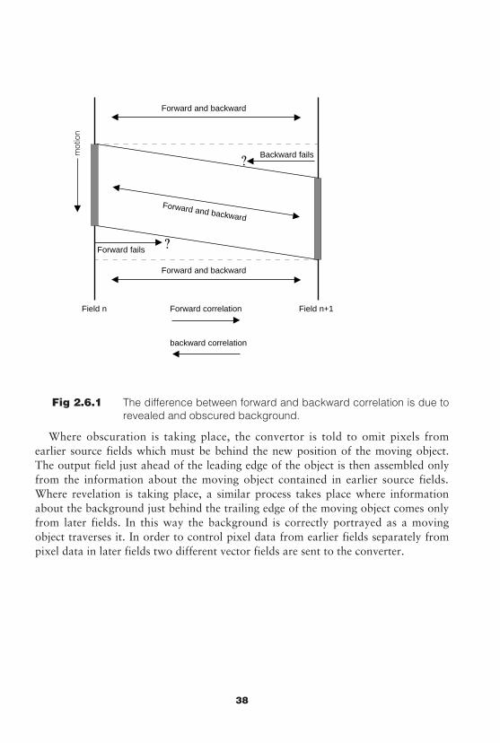
Fig 2.6.1 The difference between forward and backward correlation is due torevealed and obscured background.

Where obscuration is taking place, the convertor is told to omit pixels fromearlier source fields which must be behind the new position of the moving object.The output field just ahead of the leading edge of the object is then assembled onlyfrom the information about the moving object contained in earlier source fields.Where revelation is taking place, a similar process takes place where informationabout the background just behind the trailing edge of the moving object comes onlyfrom later fields. In this way the background is correctly portrayed as a movingobject traverses it. In order to control pixel data from earlier fields separately frompixel data in later fields two different vector fields are sent to the converter.

Forward and backward

Forward and backward

Forward and backward

Forward fails

Backward fails

Field n Field n+1Forward correlation

backward correlation

mot

ion

38

SECTION 3 – THE ALCHEMIST

The Alchemist is a high quality 24-point standards convertor which can operateas a stand alone unit. However, it is equipped with inputs to accept motion vectorsfrom an optional phase correlated motion estimation unit. Operation with andwithout motion compensation is described here.

3.1 Standards conversionStandards conversion is a form of sampling rate conversion in two or three

dimensions. The sampling rate on the time axis is the field rate and the samplingrate in the vertical axis is the number of lines in the unblanked field. The samplingrate along the line is 720 pixels per line in CCIR-601 compatible equipment. Forwidescreen or high definition signals it would be higher.

Considering first the vertical axis of the picture, taking the waveform describedby any column of pixels in the input standard, the goal is to express the samewaveform by a different number of pixels in the output standard.

This is done by interpolation. Although the input data consist of discrete samples,these actually represent a band limited analog waveform which can only join up thediscrete samples in one way. It is possible to return to that waveform by using alow-pass filter with a suitable response. An interpolator is the digital equivalent ofthat filter which allows values at points in between known samples to be computed.The operation of an interpolator is explained in the Appendix B.

There are a number of relationships between the positions of the known inputsamples and the position of the intermediate sample to be computed. The relativeposition controls the phase of the filter, which basically results in the impulseresponse being displaced with respect to the input samples. This results in thecoefficients changing. As a result a field can be expressed as any desired number oflines by performing a series of interpolations down columns of pixels.

A similar process is necessary along the time axis to change the field rate. In apractical standards convertor vertical and temporal processes are performedsimultaneously in a two dimensional filter.

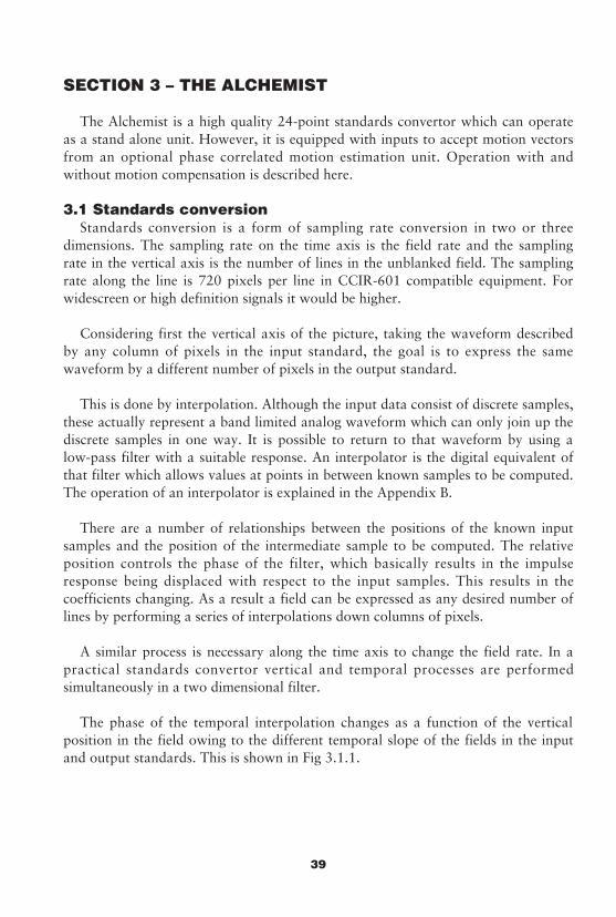
The phase of the temporal interpolation changes as a function of the verticalposition in the field owing to the different temporal slope of the fields in the inputand output standards. This is shown in Fig 3.1.1.

39

.Fig 3.1.1 The different temporal distribution of input and output fields in a

50/60Hz converter.

VerticalAxis

Timetemporal phase

temporal phase

40

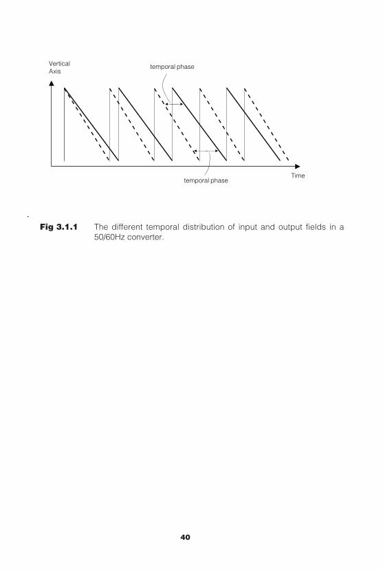
3.2 Motion CompensationIn a motion compensated standards convertor, the inter-field interpolation axis is

not aligned with the time axis in the presence of motion. Fig 3.2.1a) shows anexample without motion compensation and b) shows the same example withmotion compensation. In practice the interpolation axis is skewed by using themotion vectors to shift parts of the source fields.

Fig 3.2.1 At a) the interpolation axis is parallel with the time axis. The axismoves as shown in b) when motion compensation is used in orderto lie parallel to the axes of motion.

a) Without motioncompensation

Interpolation axis

Judder

Inputfield n+1

b) With motioncompensation

Interpolation axis

Parallel

Inputfield n

Outputfield

Inputfield n+1

Outputfield

Inputfield n

Not parallel

41

Shifting an area of a source field takes place in two stages. The displacement willbe measured in pixels, and the value is divided into the integer part, i.e the nearestwhole number of pixels, and the fractional part, i.e the sub-pixel shift. Pixels frominput fields are stored in RAM which the interpolator addresses to obtain input forfiltering. The integer part of the impulse response shift is simply added to the RAMaddress so that the pixels from the input field appear to have been shifted. Thevertical shift changes the row address and the horizontal shift changes the columnaddress. This is known as address mapping and is a technique commonly used inDVEs. Address mapping moves the image to pixel accuracy, and this stage isfollowed by using the sub-pixel shift to control the phase of the interpolator.Combining address mapping and interpolation in this way allows image areas to beshifted by large distances but with sub-pixel accuracy.

There are two ways of implementing the address mapping in a practical machinewhich are contrasted in Fig 3.2.2. In write-side shifting, the incoming source fielddata are sub-pixel shifted by the interpolator and written at a mapped write addressin the source RAM. The RAM read addresses are generated in the same way as for aconventional convertor. In read-side shifting, the source field RAM is written asnormal, but the read addresses are mapped and the interpolator is used to shift theread data to sub-pixel accuracy. Whilst the two techniques are equivalent, in factthe vectors required to control the two processes are quite different. The motionestimator computes a motion vector field in which a vector describes the distanceand direction moved by every pixel from one input field to another. This is not whatthe standards convertor requires.

42

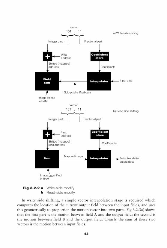
Fig 3.2.2 a Write-side modifyb Read-side modify

In write side shifting, a simple vector interpolation stage is required whichcomputes the location of the current output field between the input fields, and usesthis geometrically to proportion the motion vector into two parts. Fig 3.2.3a) showsthat the first part is the motion between field A and the output field; the second isthe motion between field B and the output field. Clearly the sum of these twovectors is the motion between input fields.

Interpolator

Coefficients

Fieldram

Shifted (mapped)address

Fractional part

Coefficientstore

Integer part

Vector

101 . 11

Writeaddress

Sub-pixel shifted data

Interpolator

Coefficients

Ram

Shifted (mapped)read address

Fractional part

Coefficientstore

Integer part

Vector

101 . 11

Mapped image

Readaddress

Sub-pixel shiftedoutput data

Image shiftedin RAM

Image not shiftedin RAM

a) Write side shifting

b) Read side shifting

Input data

43

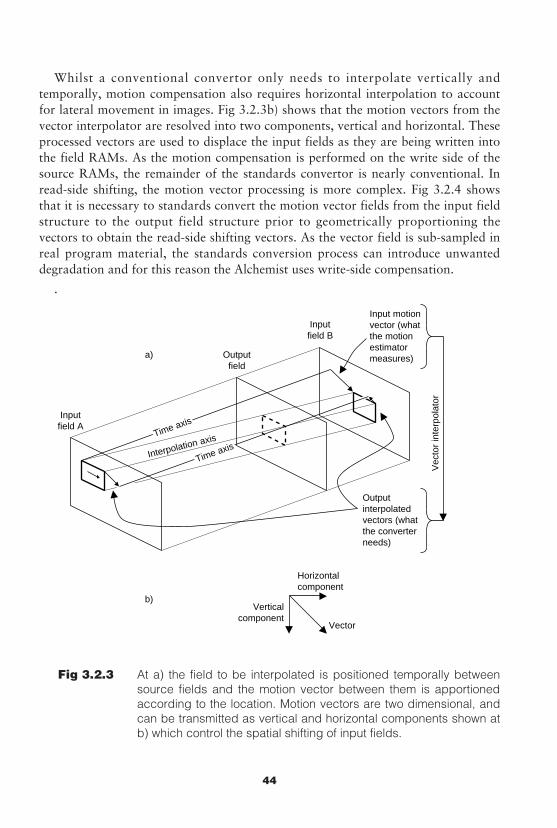
Whilst a conventional convertor only needs to interpolate vertically andtemporally, motion compensation also requires horizontal interpolation to accountfor lateral movement in images. Fig 3.2.3b) shows that the motion vectors from thevector interpolator are resolved into two components, vertical and horizontal. Theseprocessed vectors are used to displace the input fields as they are being written intothe field RAMs. As the motion compensation is performed on the write side of thesource RAMs, the remainder of the standards convertor is nearly conventional. Inread-side shifting, the motion vector processing is more complex. Fig 3.2.4 showsthat it is necessary to standards convert the motion vector fields from the input fieldstructure to the output field structure prior to geometrically proportioning thevectors to obtain the read-side shifting vectors. As the vector field is sub-sampled inreal program material, the standards conversion process can introduce unwanteddegradation and for this reason the Alchemist uses write-side compensation.

.

Fig 3.2.3 At a) the field to be interpolated is positioned temporally betweensource fields and the motion vector between them is apportionedaccording to the location. Motion vectors are two dimensional, andcan be transmitted as vertical and horizontal components shown atb) which control the spatial shifting of input fields.

Inputfield B

Inputfield A

Outputfield

Horizontalcomponent

Interpolation axis

Time axis

Input motionvector (whatthe motionestimatormeasures)

Outputinterpolatedvectors (whatthe converterneeds)

Vec

tor

inte

rpol

ator

Verticalcomponent

Vector

Time axis

a)

b)

44

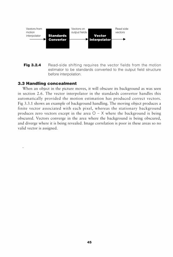
Fig 3.2.4 Read-side shifting requires the vector fields from the motionestimator to be standards converted to the output field structurebefore interpolation.

3.3 Handling concealmentWhen an object in the picture moves, it will obscure its background as was seen

in section 2.6. The vector interpolator in the standards convertor handles thisautomatically provided the motion estimation has produced correct vectors.Fig 3.3.1 shows an example of background handling. The moving object produces afinite vector associated with each pixel, whereas the stationary backgroundproduces zero vectors except in the area O – X where the background is beingobscured. Vectors converge in the area where the background is being obscured,and diverge where it is being revealed. Image correlation is poor in these areas so novalid vector is assigned.

.

Vextors frommotioninterpolator

Vectors onoutput fields

Read sidevectors

VectorInterpolator

StandardsConverter

45

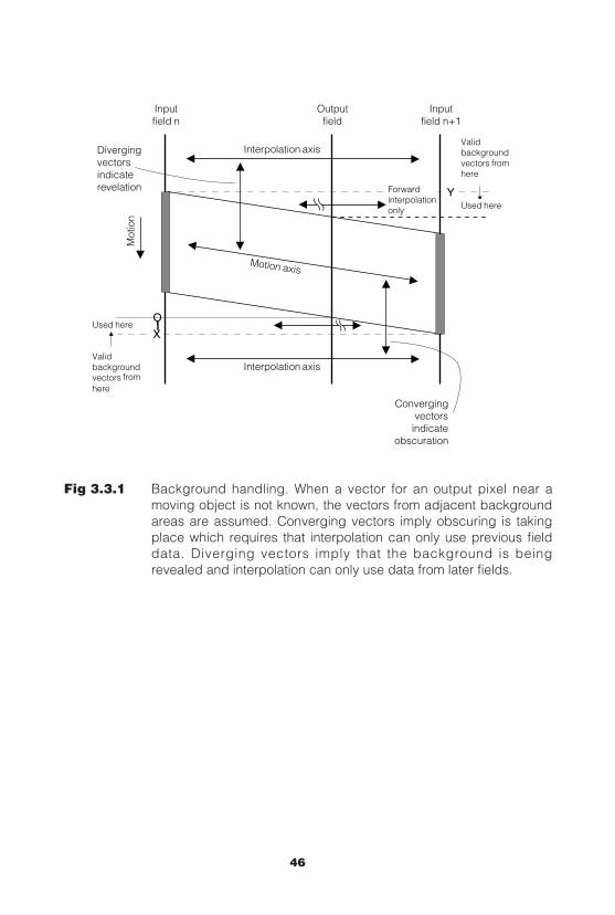
Fig 3.3.1 Background handling. When a vector for an output pixel near amoving object is not known, the vectors from adjacent backgroundareas are assumed. Converging vectors imply obscuring is takingplace which requires that interpolation can only use previous fielddata. Diverging vectors imply that the background is beingrevealed and interpolation can only use data from later fields.

Interpolation axis

Motion axis

Mot

ion

Forwardinterpolationonly

Used here

Validbackgroundvectors fromhere

Inputfield n+1

Interpolation axis

Inputfield n

Outputfield

Divergingvectorsindicaterevelation

Convergingvectorsindicate

obscuration

Validbackgroundvectors fromhere

Used here

46

An output field is located between input fields, and vectors are projected throughit to locate the intermediate position of moving objects. These are interpolated alongan axis which is parallel to the motion axis. This results in address mapping whichlocates the moving object in the input field RAMs. However, the background is notmoving and so the interpolation axis is parallel to the time axis.

The pixel immediately below the leading edge of the moving object does not havea valid vector because it is in the area O – X where forward image correlation failed.The solution is for that pixel to assume the motion vector of the background belowpoint X, but only to interpolate in a backwards direction, taking pixel data fromprevious fields. In a similar way, the pixel immediately behind the trailing edgetakes the motion vector for the background above point Y and interpolates only in aforward direction, taking pixel data from future fields. The result is that the movingobject is portrayed in the correct place on its trajectory, and the background aroundit is filled in only from fields which contain useful data. Clearly the convertor canonly handle image data from before the output field differently to that from afterthe output field if it is supplied with two sets of motion vectors.

When using write side compensation RAM data are overwritten in the area of theleading edge of a moving object as this is how concealment of the background isachieved. Clearly spurious vectors will result in undesireable overwriting. Thesolution adopted in the Alchemist is that simple overwriting is not used, but wheretwo writes take place to the same RAM address, a read modify write process isemployed in which both values contribute to the final value. Vectors haveconfidence levels attached to them. If the vector confidence is high, the overwritingvalue is favoured. If the confidence level is low, the original value is favoured.

3.5 Comparing standards convertersWhilst many items of video equipment can be tested with conventional

techniques such as frequency response and signal to noise ratio, the only way to testmotion compensated standards converters is subjectively. It is, however, importantto use program material which is sufficiently taxing otherwise performancedifferences will not be revealed.

The source of program material is important. If a tube camera is used, it willsuperimpose a long temporal aperture on the signal and result in motion blur. Thishas two effects, firstly the blur is a part of each field and so motion compensationcannot remove it. Secondly the blur may conceal shortcomings in a convertor whichbetter material would reveal. If camera motion blur is suspected, this can beconfirmed by viewing the material in freeze. The best material for testing will beobtained with CCD cameras. If shuttered cameras are available this is even better.

47

A good motion estimating convertor such as the Alchemist will maintainapparent resolution in the case of quite rapid motion with a shuttered CCD cameraas input, whereas any inaccuracy in the vectors will reduce resolution on suchmaterial.

When viewing converted material in which the cameraman pans a moving object,there will be very little judder on the panned object even without motion estimation,so the place to look is in the background, where panning causes rapid motion. Somebackgrounds conceal artifacts quite well. Grass or hedges beside race tracks do notrepresent a stringent test as they are featureless. On the other hand skiing and iceskating make good test subjects because in both there is likely to be sharply outlinedobjects in the background such as flagpoles or advertising around the rink, andthese will reveal any judder. Both are likely to result in high panning speeds, testingthe range of the motion vectors. Ballgames result in high speeds combined withsmall objects, and often contain fast pans where a camera tries to follow the ball.

Scrolling or crawling captions and credits make good test material, particularly ifcombined with fades as this tests the image correlator. Stationary captions withrapidly moving backgrounds test the obscuring /revealing process. The cautionsoutlined in section 1 regarding video from telecine machines should be heeded whenselecting demonstration material. A motion compensated standards converter doesnot contribute judder itself, but it cannot remove judder which is already present inthe source material. If use with telecine material is anticipated, it is important not tohave unrealistic expectations (See section 4.4).

48

SECTION 4 - FURTHER APPLICATIONS

Whilst standards conversion is the topic most often associated with motionestimation, it should be appreciated that this is only one application of thetechnique. Motion estimation is actually an enabling technology which findsapplication in a wide range of devices.

4.1 Slow Motion SystemsIn VTRs which are playing back at other than the correct speed, fields are

repeated or omitted to keep the output field rate correct. This results in judder onmoving objects, particularly in slow motion. A dramatic improvement in the slowmotion picture quality has been demonstrated by the Snell and Wilcox Gazelle flow-motion technology, which is a form of motion compensated standards convertorbetween the VTR and the viewer in which the input field rate is variable.

Slow-motion is one of the most stringent tests of motion estimation as a largenumber of fields need to be interpolated between the input fields and each one willhave moving objects synthesised in a different place.

4.2 Noise reductionNoise reduction in video signals works by combining together successive frames

on the time axis such that the image content of the signal is strongly reinforcedwhereas the random element in the signal due to noise does not. The noise reductionincreases with the number of frames over which the noise is integrated, but imagemotion prevents simple combining of frames. If motion estimation is available, theimage of a moving object in a particular frame can be integrated from the images inseveral frames which have been superimposed on the same part of the screen bydisplacements derived from the motion measurement. The result is that greaterreduction of noise becomes possible.

4.3 Oversampling displaysIn conventional TV displays, the marginal field rates result in flicker. If the rate at

which the display is refreshed is, for example, doubled by interpolating extra fieldsbetween those in the input signal, the flicker can be eliminated. This oversamplingtechnique is a simplified form of standards conversion which requires interpolationon the time axis. Motion compensation is necessary for the same reasons as it is instandards conversion.

49

4.4 Telecine TransferTelecine machines use a medium which has no interlace and in which the entire

image is sampled at one instant. Video is displayed with scan and interlace and sothere is a considerable disparity between the way the time axis is handled in the twoformats. As a result judder on moving parts of the image is inevitable with a directscanning telecine, particularly when 3:2 pulldown is used to obtain 60 Hz field rate.Proper telecine transfer actually requires a standards conversion process in the timeaxis which can only be done properly with motion compensation. The result is areduction in judder. Motion estimation can also be used to compensate for filmregistration errors.

These applications of motion estimation are all theoretically feasible, but are notyet all economically viable. As the real cost of digital processing power continues tofall, more of these applications will move out of the laboratory to becomecommercial devices.

The strengths of phase correlation make it the technique of choice for all of theseapplications. As high definition systems become more common, needing around fivetimes as many pixels per frame, the computational efficiency of phase correlationwill make it even more important.

50

APPENDIX AThe Fourier transform

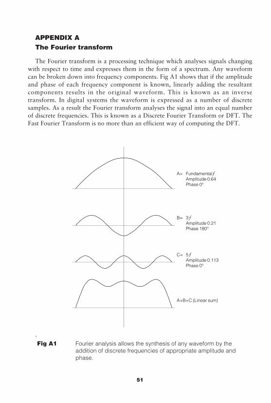
The Fourier transform is a processing technique which analyses signals changingwith respect to time and expresses them in the form of a spectrum. Any waveformcan be broken down into frequency components. Fig A1 shows that if the amplitudeand phase of each frequency component is known, linearly adding the resultantcomponents results in the original waveform. This is known as an inversetransform. In digital systems the waveform is expressed as a number of discretesamples. As a result the Fourier transform analyses the signal into an equal numberof discrete frequencies. This is known as a Discrete Fourier Transform or DFT. TheFast Fourier Transform is no more than an efficient way of computing the DFT.

.Fig A1 Fourier analysis allows the synthesis of any waveform by the

addition of discrete frequencies of appropriate amplitude andphase.

A= FundamentalAmplitude 0.64Phase 0°

B= 3Amplitude 0.21Phase 180°

C= 5Amplitude 0.113Phase 0°

A+B+C (Linear sum)

51

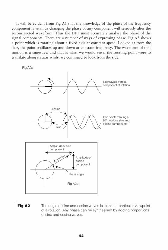
It will be evident from Fig A1 that the knowledge of the phase of the frequencycomponent is vital, as changing the phase of any component will seriously alter thereconstructed waveform. Thus the DFT must accurately analyse the phase of thesignal components. There are a number of ways of expressing phase. Fig A2 showsa point which is rotating about a fixed axis at constant speed. Looked at from theside, the point oscillates up and down at constant frequency. The waveform of thatmotion is a sinewave, and that is what we would see if the rotating point were totranslate along its axis whilst we continued to look from the side.

.Fig A2 The origin of sine and cosine waves is to take a particular viewpoint

of a rotation. Any phase can be synthesised by adding proportionsof sine and cosine waves.

Fig A2a

Sinewave is verticalcomponent of rotation

Amplitude of sinecomponent

sine

Two points rotating at90° produce sine andcosine components

cosine

Amplitude ofcosinecomponent

Amplitude

Fig A2b

Phase angle

52

One way of defining the phase of a waveform is to specify the angle throughwhich the point has rotated at time zero (T=0).

If a second point is made to revolve at 90 degrees to the first, it would produce acosine wave when translated. It is possible to produce a waveform having arbitraryphase by adding together the sine and cosine wave in various proportions andpolarities. For example adding the sine and cosine waves in equal proportion resultsin a waveform lagging the sine wave by 45 degrees.

Fig A2b shows that the proportions necessary are respectively the sine and thecosine of the phase angle. Thus the two methods of describing phase can be readilyinterchanged.

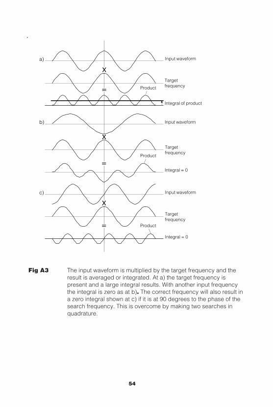
The Fourier transform analyses the spectrum of a block of samples by searchingseparately for each discrete target frequency. It does this by multiplying the inputwaveform by a sine wave having the target frequency and adding up or integratingthe products.

Fig A3a) shows that multiplying by the target frequency gives a large integralwhen the input frequency is the same, whereas Fig A3b) shows that with a differentinput frequency (in fact all other different frequencies) the integral is zero showingthat no component of the target frequency exists. Thus from a real waveformcontaining many frequencies all frequencies except the target frequency areexcluded.

53

.

Fig A3 The input waveform is multiplied by the target frequency and theresult is averaged or integrated. At a) the target frequency ispresent and a large integral results. With another input frequencythe integral is zero as at b). The correct frequency will also result ina zero integral shown at c) if it is at 90 degrees to the phase of thesearch frequency. This is overcome by making two searches inquadrature.

Input waveform

Integral of product

Targetfrequency

Input waveform

Targetfrequency

Integral = 0

Input waveform

Targetfrequency

Integral = 0

Product

Product

Product

a)

b)

c)

54

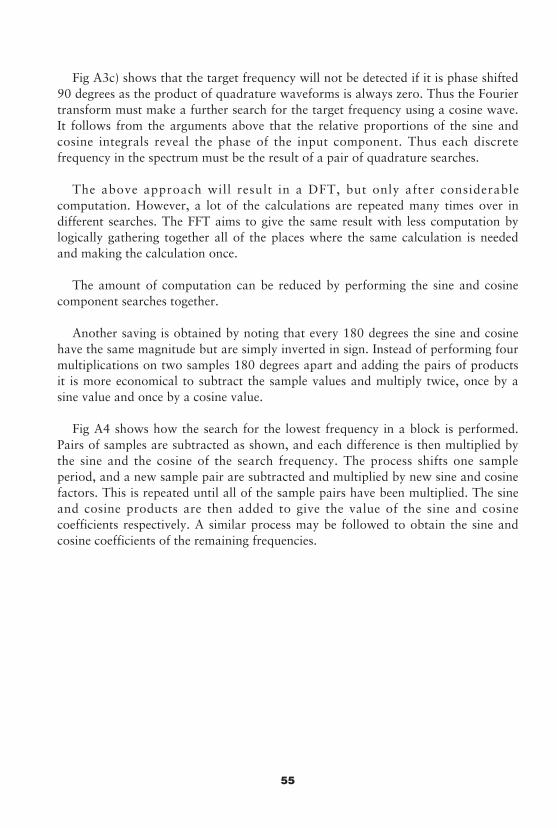
Fig A3c) shows that the target frequency will not be detected if it is phase shifted90 degrees as the product of quadrature waveforms is always zero. Thus the Fouriertransform must make a further search for the target frequency using a cosine wave.It follows from the arguments above that the relative proportions of the sine andcosine integrals reveal the phase of the input component. Thus each discretefrequency in the spectrum must be the result of a pair of quadrature searches.

The above approach will result in a DFT, but only after considerablecomputation. However, a lot of the calculations are repeated many times over indifferent searches. The FFT aims to give the same result with less computation bylogically gathering together all of the places where the same calculation is neededand making the calculation once.

The amount of computation can be reduced by performing the sine and cosinecomponent searches together.

Another saving is obtained by noting that every 180 degrees the sine and cosinehave the same magnitude but are simply inverted in sign. Instead of performing fourmultiplications on two samples 180 degrees apart and adding the pairs of productsit is more economical to subtract the sample values and multiply twice, once by asine value and once by a cosine value.

Fig A4 shows how the search for the lowest frequency in a block is performed.Pairs of samples are subtracted as shown, and each difference is then multiplied bythe sine and the cosine of the search frequency. The process shifts one sampleperiod, and a new sample pair are subtracted and multiplied by new sine and cosinefactors. This is repeated until all of the sample pairs have been multiplied. The sineand cosine products are then added to give the value of the sine and cosinecoefficients respectively. A similar process may be followed to obtain the sine andcosine coefficients of the remaining frequencies.

55

.

Fig A4 An example of a filtering search. Pairs of samples are subtractedand multiplied by sampled sine and cosine waves. The productsare added to give the sine and cosine components of the searchfrequency.

Xcos 135°

Inputsamples

Xsin 135°

0 1 2 3 4 5 6 7

Targetfrequency

Sinecomponent

Cosinecomponent

Xcos 90°

Xcos 45°

Xsin 90°

Xsin 45°

Xsin 0°

Xcos 0°

0 45 90 135 180

56

In practice some tricks are used to further reduce computation, but as the result isthe same it is not necessary to go into such details here. As a result of the FFT, thesine and cosine components of each frequency are available. For use with phasecorrelation it is necessary to convert to the alternative means of expression, i.e phaseand amplitude.

The number of frequency coefficients resulting from a DFT is equal to thenumber of input samples. If the input consists of a larger number of samples it mustcover a larger area of the screen, but its spectrum will be known more finely.

Thus a fundamental characteristic of such transforms is that the more accuratelythe frequency and phase of a waveform is analysed, the less is known about wheresuch frequencies exist on the spatial axis.

57

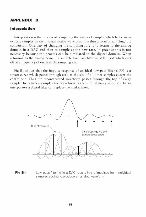
APPENDIX B

Interpolation

Interpolation is the process of computing the values of samples which lie betweenexisting samples on the original analog waveform. It is thus a form of sampling rateconversion. One way of changing the sampling rate is to return to the analogdomain in a DAC and then to sample at the new rate. In practice this is notnecessary because the process can be simulated in the digital domain. Whenreturning to the analog domain a suitable low pass filter must be used which cutsoff at a frequency of one half the sampling rate.

Fig B1 shows that the impulse response of an ideal low-pass filter (LPF) is asinx/x curve which passes through zero at the site of all other samples except thecentre one. Thus the reconstructed waveform passes through the top of everysample. In between samples the waveform is the sum of many impulses. In aninterpolator a digital filter can replace the analog filter.

Fig B1 Low pass filtering in a DAC results in the impulses from individualsamples adding to produce an analog waveform

Zero crossings are onesample period apart

Sum of impulses

58

.

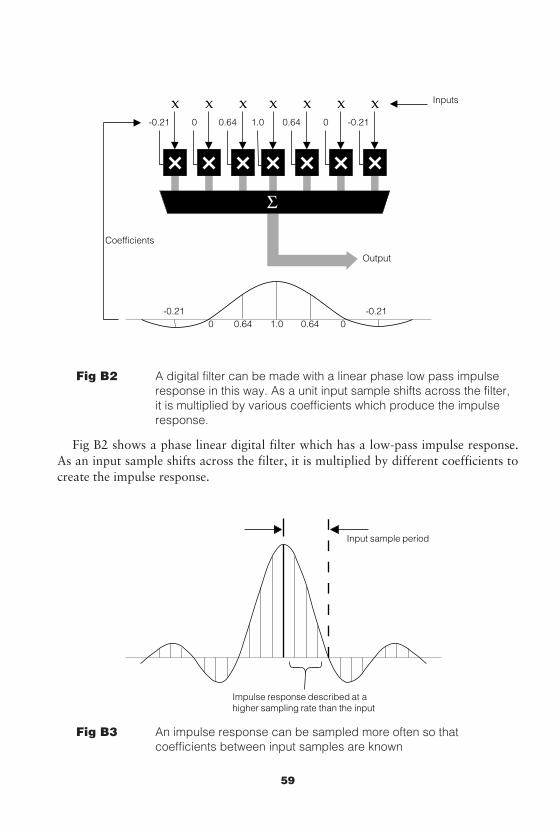
Fig B2 A digital filter can be made with a linear phase low pass impulseresponse in this way. As a unit input sample shifts across the filter,it is multiplied by various coefficients which produce the impulseresponse.

Fig B2 shows a phase linear digital filter which has a low-pass impulse response.As an input sample shifts across the filter, it is multiplied by different coefficients tocreate the impulse response.

Fig B3 An impulse response can be sampled more often so that coefficients between input samples are known

Impulse response described at ahigher sampling rate than the input

Input sample period

Inputs

Coefficients

Output

-0.21 0 0.64 1.0 00.64 -0.21

-0.210 0.64 1.0 0.64 0

-0.21

59

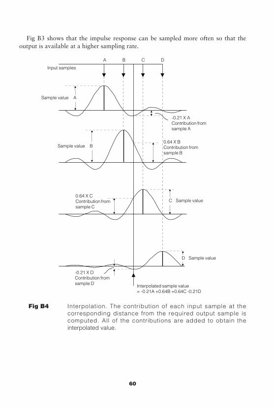
Fig B3 shows that the impulse response can be sampled more often so that theoutput is available at a higher sampling rate.

Fig B4 Interpolation. The contribution of each input sample at thecorresponding distance from the required output sample iscomputed. All of the contributions are added to obtain theinterpolated value.

Input samples

-0.21 X AContribution fromsample A

Sample value A

Sample value B

C Sample value

D Sample value

0.64 X BContribution fromsample B

0.64 X CContribution fromsample C

-0.21 X DContribution fromsample D

A B C D

Interpolated sample value= -0.21A +0.64B +0.64C -0.21D

60

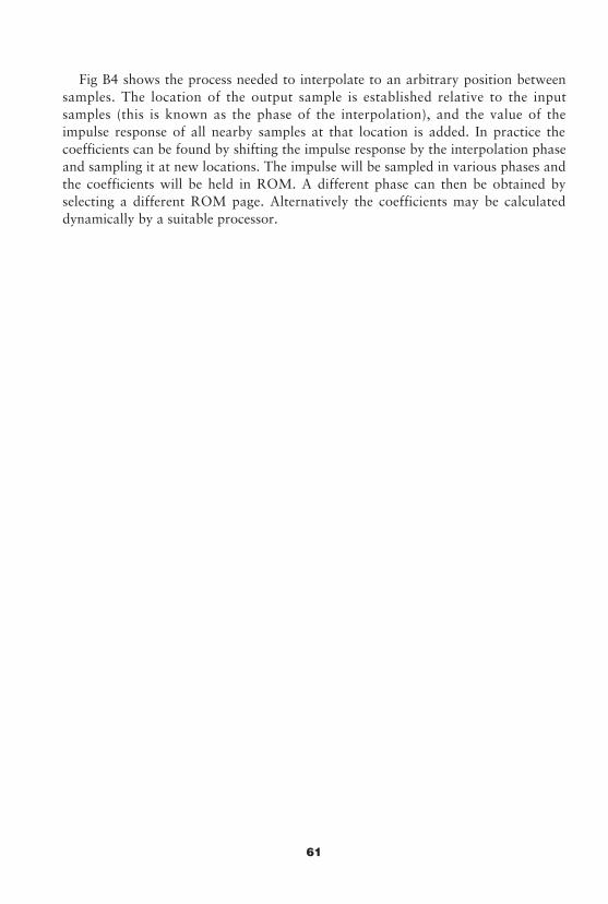
Fig B4 shows the process needed to interpolate to an arbitrary position betweensamples. The location of the output sample is established relative to the inputsamples (this is known as the phase of the interpolation), and the value of theimpulse response of all nearby samples at that location is added. In practice thecoefficients can be found by shifting the impulse response by the interpolation phaseand sampling it at new locations. The impulse will be sampled in various phases andthe coefficients will be held in ROM. A different phase can then be obtained byselecting a different ROM page. Alternatively the coefficients may be calculateddynamically by a suitable processor.

61

Published by Snell & Wilcox Ltd.

Durford Mill

Petersfield

Hampshire

GU13 5AZ

Tel: +44 (0) 703 821188

Fax: +44 (0) 703 821199

Copyright © Snell & Wilcox 1994

Text and diagrams from this publication may be reproduced providing acknowledgement is

given to Snell & Wilcox.

62