The equilibrium consequences of indexing∗

Philip Bond† Diego Garcıa‡

First draft: September 2016

This draft: July 2020

Abstract

We develop a benchmark model to study the equilibrium consequences of indexing

in a standard rational expectations setting. Individuals incur costs to participate in

financial markets, and these costs are lower for individuals who restrict themselves

to indexing. A decline in indexing costs directly increases the prevalence of index-

ing, thereby reducing the price efficiency of the index and augmenting relative price

efficiency. In equilibrium, these changes in price efficiency in turn further increase

indexing, and raise the welfare of uninformed traders. For well-informed traders, the

share of trading gains stemming from market timing increases relative to stock selection

trades.

JEL classification: D82, G14.

Keywords: indexing, welfare.

∗We thank seminar audiences at Baruch College, BI Oslo, Boston College, the Hanqing Institute of RenminUniversity, Hong Kong University, Insead, LBS, LSE, MIT, Michigan State University, Notre Dame, NYU,Stanford, the University of Alberta, UC San Diego, the University of Chicago, the University of Maryland,the University of North Carolina, the University of Rochester, UT Austin, the University of Utah, and theUniversity of Virginia and for helpful comments. Any remaining errors are our own.

†Philip Bond, University of Washington, Email: apbond@uw.edu; Webpage: http://faculty.

washington.edu/apbond/.‡Diego Garcıa, University of Colorado Boulder, Email: diego.garcia@colorado.edu; Webpage: http:

//leeds-faculty.colorado.edu/garcia/.

1 Introduction

The standard investment recommendation that financial economists offer to retail investors

it to purchase a low-fee index mutual fund or exchange-traded fund (ETF), a strategy often

describe as “index investing,” or simply “indexing.” An increasing number of indexing

products are available, and are increasingly inexpensive and accessible, and more and more

investors follow this advice.1 In this paper, we develop a benchmark model to analyze

the equilibrium consequences of a decrease in indexing costs, paying particular attention to

consequences for participation and welfare.

Our model has the following three features, all of which are necessary for the topic at

hand. First, and because much of the discussion of indexing revolves around retail investors,

some agents in our model have much less information about future asset cash flows than

others. Second, while agents seek trading profits, they also have other trading motives;2 we

model these as stemming from a desire to reallocate risk from non-financial income, with the

effect on agents’ desired trades resembling discount rate shocks. Third, there are costs to

participating in financial markets, which are potentially lower for investors who index. We

characterize what happens as indexing costs fall.

The direct consequence of a fall in indexing costs is, naturally, to draw investors into in-

dexing, and away from both more active trading strategies and non-participation in financial

markets. The marginal investor who switches from non-participation to indexing is relatively

uninformed. Similarly, the marginal investor who switches out of active trading into indexing

is someone who was uninformed relative to other active traders. So the direct consequence

of falling indexing costs is to reduce the price efficiency of the index and introduce a common

“noise” factor to stock prices of firms covered by the index,3 while simultaneously reducing

“liquidity” in individual stocks.

The central questions we ask in this paper are: What equilibrium effects follow from

these direct consequences of a fall in indexing costs? And what is the net effect on investors’

welfare? In particular, do equilibrium forces dampen the direct consequences, or are the

direct consequences instead self-reinforcing?

We find that the direct consequences are self-reinforcing. Although the reduction in price

efficiency associated with indexing may sound undesirable, investor welfare increases, even

for the least informed investors, as we discuss below. The increase in the welfare of indexing

1See, for example, French (2008) and Stambaugh (2014).2Absent such motives, the no-trade theorem would apply.3See evidence in, for example, Ben-David, Franzoni, and Moussawi (2018). To anticipate our formal

analysis: The reason why the investors who switch from active trading to indexing do not increase theaverage informedness of investors who trade the index is that, even before the switch, they were alreadytrading the index—either explicitly via an index fund or ETF, or implicitly via a basket of individual stocks.

1

investors draws in more relatively uninformed investors, amplifying the original effect.

Conversely, the direct consequence of relatively uninformed investors switching from ac-

tive trading to index investing is to increase the price efficiency of individual stock prices.

Although this sounds desirable, it reduces investor welfare. This induces yet more investors

to abandon active trading, again amplifying the original effect.

As the above discussion suggests, our key analytical result is that increases in participa-

tion in the market for a financial asset increase the welfare of those already participating.

Put differently, participation decisions are strategic complements.4 The underlying economic

force is that an individual investor prefers to trade in a market in which the average investor

is relatively uninformed; since the marginal investor is less informed than the average in-

vestor, this generates strategic complementarity. Although it may seem intuitive that an

investor prefers his average counterparty to be uninformed, this same force leads to prices

that are more divorced from cash flows, i.e., lower price efficiency, which is often interpreted

as being undesirable. Concretely, lower price efficiency in our framework means that prices

are more exposed to fluctuations in expected non-financial income that investors wish to

partially hedge, i.e., fluctuations in discount rates. As such, establishing an investor’s pref-

erence for less informed counterparties entails establishing that the benefits of a less informed

average counterparty exceed the costs of lower price efficiency.5 Perhaps surprisingly, and

despite the fact that we work with a canonical model of the type introduced by Diamond

and Verrecchia (1981), this analysis has not been conducted by the existing literature.

The central empirical predictions of our analysis are about price efficiency. As indexing

costs fall, and indexing increases, price efficiency of the index as a whole falls, while the

relative price efficiency of individual stocks increases. Moreover, price efficiency is lower for

stocks covered by the index than for those outside. It further follows that index reversals

become more pronounced, and a greater fraction of the trading gains of relatively informed

investors are attributable to “market timing” strategies as opposed to “stock selection”

strategies. Section 5 reviews empirical support for these findings.

Asides from its implications for the equilibrium effects of indexing, our paper also con-

tributes to the wider debate of the extent to which the financial sector contributes to social

welfare (see, e.g, Baumol (1965)). In particular, we work with a canonical model in which

a financial market exists because it facilitates risk-sharing, and show that informed trading

4Grossman and Stiglitz (1980) analyze traders’ decisions to become informed, taking the set of tradingagents as given, and show that information acquisition decisions are strategic substitutes: the incrementaltrading profits from private information decline as more traders become informed. In contrast, we considera setting without exogenous noise traders, and analyze traders’ participation decisions.

5This result is related to the so-called “Hirshleifer effect” (Hirshleifer (1971)), but does not follow directlyfrom it; see subsection 3.1 below, and also related discussions in Marın and Rahi (1999) and Dow and Rahi(2003).

2

generally worsens this risk-sharing function, while uninformed trading improves it. In Sec-

tion 7 we also explore an extension of our baseline model in which the information produced

by financial markets guides resource allocation decisions (see Bond, Goldstein, and Edmans

(2012) for a survey), and in doing so formalize a positive welfare effect of the increase in the

relative price efficiency that follows from lower indexing costs.

Related literature: In its general theme, our analysis is related to papers such as Sub-

rahmanyam (1991), Cong and Xu (2019), Stambaugh (2014), and Bhattacharya and O’Hara

(2018). Subrahmanyam (1991) models the introduction of index futures, while Cong and Xu

(2019) and Bhattacharya and O’Hara (2018) model the introduction of ETFs. An impor-

tant assumption in all three papers is how the introduction of a new financial product affects

the allocation of “noise” or liquidity traders across assets.6 Stambaugh (2014) analyzes the

effects of an exogenous decline in noise traders for financial markets, and in particular, for

actively managed investment funds.7 Relative to all these papers, we model the behavior

of all financial market participants, and in particular, analyze how a fall in indexing costs

affects participation decisions and welfare.

In an independent, contemporaneous, and complementary paper, Baruch and Zhang

(2018) likewise study the equilibrium consequence of indexing, though from a very differ-

ent perspective. They consider a multi-asset version of Grossman (1976), so that without

indexing prices fully reveal agents’ private signals. In this setting they show that an exoge-

nous increase in indexing reduces the amount of information prices contain about individual

assets, while the amount of information prices contain about aggregates is unaffected.

We have deliberately based our analysis on the canonical model of financial markets of

Diamond and Verrecchia (1981). Like Grossman and Stiglitz (1980), Hellwig (1980), and

Admati (1985), these authors analyze trade between differentially informed agents, but dif-

ferent from these papers, there are no exogenous “noise” or “liquidity” trades. Instead,

agents have heterogeneous and privately observed exposures to risk. Consequently, finan-

cial markets hold the potential to increase welfare by allowing agents to redistribute risk.

Perhaps surprisingly, and although a model of this type has been analyzed by a significant

number of authors, results on welfare are scarce.8 One significant algebraic complication

6Subrahmanyam (1991), and Cong and Xu (2019) allow for optimization by a subset of these traders.7Also related is Garleanu and Pedersen (2018), who among other things consider an investor’s choice

between actively and passively managed funds. However, they consider a financial market with a single riskyasset, making it hard to consider “indexing.”

8For results on the effect of information on welfare in different equilibrium models of financial markets,see, for example, Schlee (2001) and Kurlat (2019). The former paper analyzes the value of public signals in asetting in which individual endowments are public once they are realized, and so trades can be conditioned onthem, and characterizes conditions in which improvements in public information cause a Pareto deterioration.In contrast, in our setting (inherited from Diamond and Verrecchia (1981)), individual signals are private,

3

in characterizing welfare is that, when combined with the asset price, each agent’s private

exposure shock contains information about expected asset payoffs. To avoid this compli-

cation, Verrecchia (1982) and Diamond (1985) both consider a sequence of economies in

which the variance of each individual’s exposure shock grows with the number of agents,

and directly study the limit of this sequence. In the limit economy, each agent’s exposure

shock has infinite variance, and so expected utility prior to the realization of the exposure

shock is undefined, in turn making it impossible to analyze participation decisions prior to

the realization of exposure shocks.9

In an independent, contemporaneous, and complementary paper, Kawakami (2017) also

makes progress in characterizing welfare in a setting along the lines of Diamond and Ver-

recchia (1981). Whereas we focus on an economy with a continuum of agents and allow for

heterogeneity in the precision of signals about cash flows that agents observe, thereby al-

lowing us to consider the effect an increase in participation by relatively uninformed agents,

Kawakami instead considers a finite-agent economy with homogeneous signal precisions, in

which an increase in the size of the market is associated with better diversification of indi-

vidual exposure shocks. Analytically, we make more explicit use than Kawakami of market-

clearing conditions, which allows us to incorporate heterogeneity in signal precisions in a

tractable way.

Marın and Rahi (1999) obtain welfare results in a relatively specialized setting: there

are two classes of agents, one class of which sees identical signals about asset payoffs and

private endowments, and another class of completely uninformed agents. Moreover, the

traded asset is in zero net supply. Dow and Rahi (2003) also analyze welfare, and obtain

some tractability by inserting a risk-neutral market maker into the economy, which reduces

the applicability of the model for analyzing aggregate financial markets. In closely related

settings, Medrano and Vives (2004) argue that “the expressions for the expected utility of

a hedger . . . are complicated,” whereas Kurlat and Veldkamp (2015) write that “there is no

closed-form expression for investor welfare.” The complications, common to our model as

well, stem from the role of exposure shocks as signals about asset cash flows, on top of the

standard risk sharing role that motivates trade.

and individual endowments are likewise private, even after they are realized. The latter paper analyzeswhat is essentially an origination market in which sellers are strictly better informed than buyers, andcharacterizes the ratio of the social to private value of buyer information. In this setting, improvements inseller information reduce adverse selection, and so the social value of information is positive. In contrast,in our setting improvements in trader information do not necessarily reduce adverse selection, and ourresults imply that improvements in information of a positive measure of agents reduce the welfare of allcounterparties.

9If instead one modeled participation decisions as being made after the exposure shock, then almost allagents would participate, since their exposure shocks are so large.

4

Finally, we emphasize that we examine “indexing” in the sense of a “passive” investment

strategy based on an index. Other authors have analyzed the distinct topic of the role of

indices as benchmarks that affect the compensation of fund managers: see, e.g., Admati and

Pfleiderer (1997), Basak and Pavlova (2013), Buffa, Vayanos, and Woolley (2019).

2 The model

2.1 Preferences, assets, endowments, information

We work with a version of Diamond and Verrecchia (1981) in which there is a unit interval

of agents (see Ganguli and Yang (2009) and Manzano and Vives (2011)), i ∈ [0, 1], and

multiple assets. We emphasize that this is a canonical setting, in which risk-sharing benefits

lead to gains from trade, which in turn allows for informed trading. Indeed, we are unable

to think of a simpler or more standard framework that still contains the three key features

discussed in the introduction.

Each agent i has preferences with constant absolute risk aversion (CARA) over terminal

wealth Wi, and a coefficient of absolute risk aversion of γ. There are m risky assets available

for trading; and also a risk-free asset that is in perfectly elastic supply and has a net return

that we normalize to 0.10 Each asset k ∈ {1, . . . , m} produces a payoff given by random

variable Xk, with variance τ−1X . All exogenous random variables in the model are normally

distributed and mutually independent. Each agent’s initial endowment of each asset is S.

We characterize the competitive equilibrium of the economy, where agents are small relative

to the market, and act as price-takers. The equilibrium price of asset k is Pk.

In addition, agents have other sources of income (e.g., labor income, non-traded capital

income) that are correlated with the cash flows of the risky assets. For simplicity, we assume

the correlation is perfect. Specifically, let Zk and uik be random variables, and define agent

i’s income from sources other than the risky assets by

m∑

k=1

(

Zk + uik

)

Xk. (1)

Here, Zk + uik represents agent i’s non-financial exposure to the cash flow risk Xk. Agent

i privately observes the sum Zk + uik, but not its individual components Zk and uik. So

agents know their own income exposures Zk+ uik, but remain uncertain about the aggregate

10Alternatively, one can assume the risk-free asset is in zero net supply, and interpret the prices of riskyassets as forward prices (i.e., the amount of certain wealth that will be exchanged for the risky asset’s payoffat the terminal date). In this case, the market for the risk-free asset clears by Walras’s Law.

5

component of other agents’ exposures, Zk. The variances of Zk and uik are τ−1Z and τ−1

u

respectively, and E

[

Zk

]

= E [uik] = 0.

Our environment is symmetric across assets; this considerably simplifies the analysis

because it makes possible the change of basis that we describe in subsection 2.3. Moreover,

agents have the same risk aversion, initial asset endowments, and ex ante exposures to

other sources of risk, though they differ in their access to information, as described below.

These agent-symmetry properties are important in allowing us to tractably characterize the

expected utility from participation in financial markets, and hence participation decisions.

That said, the agent-symmetry assumptions can be relaxed to some extent. For example,

it is straightforward to instead assume that some agents have greater initial endowments of

financial assets but smaller ex ante exposures to non-financial risk, provided the combined

ex ante financial and non-financial exposure remains constant across agents. Similarly, we

could also generalize our analysis to allow some agents to have greater initial endowments

of financial assets but lower risk aversions, provided the two sources of variation offset each

other in an appropriate way.

Gains from trade stem from agents’ differential and privately observed realized exposures

Zk + uik. In equilibrium, aggregate exposures Zk affect prices, and so fluctuations in Zk are

effectively fluctuations in discount rates. It is also worth noting that one can give a more

behavioral interpretation to Zk + uik; looking ahead to agents’ optimal trade (11), Zk + uik

can be interpreting simply as a shock to agent i’s desired holding of asset k, independent of

the source of this shock.

The terminal wealth of agent i is determined by the combination of trading profits, payoffs

from initial asset endowments, and other income (1). For notational convenience, define

eik = S + Zk + uik

to represent agent i’s net exposure to cash flow Xk, stemming from the combination of initial

asset holdings and non-financial exposure.

We denote by θik agent i’s trade of asset k. The terminal wealth of an agent who makes

the vector of trades θi is

W(

θi, ei

)

≡m∑

k=1

θik

(

Xk − Pk

)

+sikXik+(

Zk + uik

)

Xik =

m∑

k=1

(

θik + eik

)(

Xk − Pk

)

+eikPk.

(2)

Prior to trading, each agent i observes private signals of the form

yik = Xk + ǫik,

6

where ǫik is a random variable with mean 0 and variance τ−1i .11

The precisions τ−1i of private signals are heterogeneous across agents, so that some agents

are more informed than others. Without loss of generality, we order agents so that signal

precision τi is decreasing in i; and for simplicity, we assume τi is strictly decreasing.12

An agent’s information set at the time of trading is hence the triple ofm-vectors(

yi, ei, P)

,

which consists of signals about cash flows yi; exposures ei; and prices P .

2.2 Indexing and participation

Agents incur a cost κ > 0 of fully participating in financial markets, reflecting a combination

of information collection and processing costs, psychic costs, expected trading costs, and the

cost of potentially trading in a less than optimal way. Agents make participation decisions

prior to observing any of(

yi, ei, P)

. This timing assumption for the participation decision is

important for tractability, since it ensures that all random variables are normally distributed

at the trading stage.

In addition to fully participating in financial markets, agents have the option of partici-

pating only via trading an “index” asset. The index covers the first l ≤ m of the m assets,

where we assume that l is a power of 2 (this greatly enhances tractability, as will become

clear in the next subsection). Since all assets have the same supply S, equal-weighted and

value-weighted indices coincide,13 and the cash flow produced by the index is

X1 ≡ l−1

2

l∑

k=1

Xk, (3)

where l1

2 is an index divisor, chosen so that var (X1) = τ−1X .

Formally, we denote by Θl the set of trade vectors that are feasible for an indexing agent,

11Note that an agent i has the same quality signal about all assets. We leave the interaction of heterogeneityof signal precision across assets with heterogeneity of signal precisions across agents for future research.

12Formally, our model is one in which all agents either invest directly in individual stocks, or else invest viapassive index funds (see below). An alternative interpretation is that agents with a low i index (and henceprecise signals) are relatively good at identifying skilled mutual and hedge funds (Garleanu and Pedersen(2018)), and the direct investments in the model are made through such intermediaries. Looking ahead, andas one would expect, agents’ desired trades depend on their exposure realizations. So in the intermediatedinvestment interpretation just described, agents would also pay attention to general “styles” of funds, inaddition to the skill of managers. See also Garcıa and Vanden (2009).

13The index defined in (3) is an equal-weighted index. It is also a value-weighted index, as follows. Sincean agent who trades the index trades an equal number of units of the l assets in the index, the value share

of the trade in asset k ≤ l to the agent’s total trades is Pk∑lj=1

Pj. Because the assets have the same market

supply S, this coincides with the value share of asset k in the portion of the market covered by the index,

i.e., SPk∑lj=1

SPj.

7

i.e., trades in which agent i buys or sells equal amounts of all assets in the index, and zero

units of any asset outside the index:

Θl ={

θi ∈ Rm : θij = θik for any j, k ∈ {1, . . . , l} and θik = 0 for k > l

}

.

The advantage of participating in financial markets only via indexing is that the partici-

pation cost is lower, which we denote by κ1 ∈ (0, κ). The lower participation cost of indexing

reflects lower trading costs, because of the availability of low cost index mutual funds and

exchange traded funds (ETFs); lower cognitive demands and attention costs; and lower in-

formation costs, since as our formal analysis will show, a sufficient statistic for agent i’s

private information under indexing is the average signal for assets in the index, 1l

∑lk=1 yik,

which can be interpreted as agent i restricting attention to broad economic aggregates.

Looking ahead, the main comparative static we will be interested in is a fall in the cost

of indexing κ1. This corresponds to falling fees, greater availability, and greater awareness

of products such as low-cost index funds and ETFs. It may also reflect an increase in public

awareness of the standard advice given by finance academics.

Finally, individuals i who do not participate in financial markets at all pay no participa-

tion cost, but do not trade, i.e., θik = 0 for all assets k.

The definition of an equilibrium in terms of pricing, participation decisions, and trading

strategies is standard. However, we postpone a formal statement of equilibrium conditions

until subsection 2.4. This allows us to give the definition directly in terms of a spanning set

of synthetic assets, which we introduce next, and use to conduct our analysis.

2.3 Disentangling markets

Although the fundamentals of different assets are independent in all dimensions, the presence

of indexing agents links the prices of distinct assets. For example, if j and k are two distinct

assets covered by the index, then an indexing agent’s exposure eij to cash flow risk Xj affects

the agent’s desired trade of asset k as well as of asset j.

Because of the entanglement that indexing produces between different assets covered by

the index, it is analytically very convenient to change basis and study the economy in terms

of a set of synthetic assets that are mutually independent even in the presence of indexers.14

The case of two assets (l = m = 2) is simple. The first synthetic asset is the index

portfolio, X1 = 1√2

(

X1 + X2

)

. The second synthetic asset is X2 = 1√2

(

X1 − X2

)

, which

can be labeled a “spread” asset, as it allows agents to trade on the relative mispricing between

14This change of basis is not essential to solve for equilibrium prices; see Admati (1985)’s analysis of amulti-asset version of Hellwig (1980).

8

assets 1 and 2. We next generalize this construction to l > 2 assets in the index. We first

give a representative example, and then formalize the change of basis.

Example: Suppose there are m = 5 assets and the index covers the first l = 4. Then

consider the following set of 5 synthetic assets, where the 1st synthetic asset is the index

asset, and pays X1 as defined in (3); the 5th synthetic asset coincides with the underlying

asset 5, i.e., it pays X5 = X5; and the remaining 3 synthetic assets are long-short positions

in assets covered by the index, and pay X2, X3, X4 defined by

X2 =1

2

(

X1 + X3 − X2 − X4

)

,

X3 =1

2

(

X1 + X2 − X3 − X4

)

,

X4 =1

2

(

X1 + X4 − X2 − X3

)

.

The five synthetic assets span the underlying assets Xk. Moreover, they are uncorrelated

(i.e., cov (Xj, Xk) = 0 for all j, k), and each has variance τ−1X . Note that E [X1] =

124E[

X1

]

=√4E[

X1

]

, while E [Xj ] = 0 for synthetic assets j = 2, 3, 4. Similarly the per-agent endow-

ment of the index synthetic asset 1 is 2S =√4S, while synthetic assets j = 2, 3, 4 are in

zero net supply.

Everything about the example extends to the general case (formally, see Lemmas A-1

and A-2 in appendix). Specifically, we construct l synthetic assets to span assets 1, . . . , l.

Synthetic asset 1 is the index asset that pays X1 as defined in (3), with E [X1] =√lE[

X1

]

and per-agent endowment S1 ≡√lS. Synthetic assets j = 2, . . . , l have payoffs denoted Xj ,

with E [Xj ] = 0 and per-capita endowment Sj ≡ 0. For assets j > l outside the index we

simply define Xj = Xj, i.e., the synthetic and fundamental asset coincide. The correlation

of any pair of synthetic assets is 0. The variance of each synthetic asset is τ−1X .

In general, we use tildes to denote quantities related to fundamental assets, and the

absence of a tilde to denote quants related to synthetic assets. For example, P is the vector

of prices of synthetic assets, and the vector θi is agent i’s portfolio of synthetic assets. So,

in terms of synthetic assets, the terminal wealth of agent i given the vector of exposures ei

and portfolio θi is

W (θi, ei) =m∑

k=1

(θik + eik) (Xk − Pk) + eikPk.

Consequently, to solve for equilibrium prices and welfare, we work directly with the

synthetic assets described above. By construction, the synthetic assets are independent of

each other in all respects. Moreover, and importantly, indexing corresponds simply to the

9

constraint that an agent can trade only synthetic asset 1, with no trade of any of the other

synthetic assets. This means we can analyze the equilibrium in the market for each synthetic

asset in isolation (given CARA preferences). Formally, we denote the set of trades available

to agents who pay the reduced participation cost κ1 by Θ1 ≡ {θi ∈ Rm : θik = 0 if k 6= 1}.

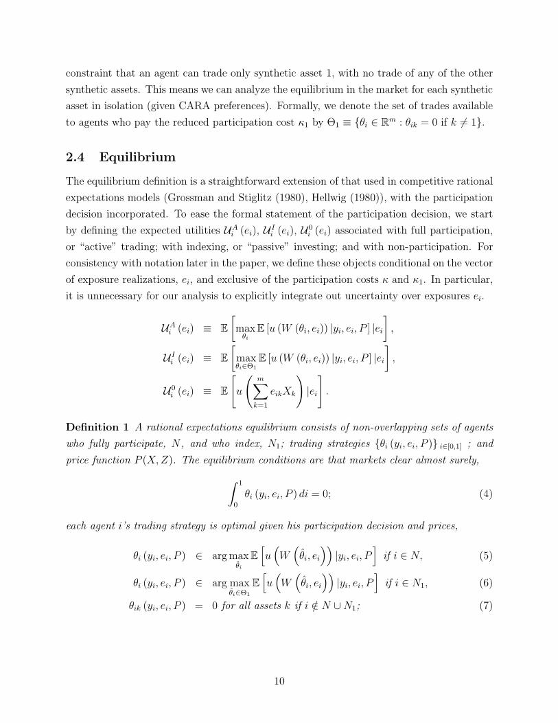
2.4 Equilibrium

The equilibrium definition is a straightforward extension of that used in competitive rational

expectations models (Grossman and Stiglitz (1980), Hellwig (1980)), with the participation

decision incorporated. To ease the formal statement of the participation decision, we start

by defining the expected utilities UAi (ei), U I

i (ei), U0i (ei) associated with full participation,

or “active” trading; with indexing, or “passive” investing; and with non-participation. For

consistency with notation later in the paper, we define these objects conditional on the vector

of exposure realizations, ei, and exclusive of the participation costs κ and κ1. In particular,

it is unnecessary for our analysis to explicitly integrate out uncertainty over exposures ei.

UAi (ei) ≡ E

[

maxθi

E [u (W (θi, ei)) |yi, ei, P ] |ei]

,

U Ii (ei) ≡ E

[

maxθi∈Θ1

E [u (W (θi, ei)) |yi, ei, P ] |ei]

,

U0i (ei) ≡ E

[

u

(

m∑

k=1

eikXk

)

|ei]

.

Definition 1 A rational expectations equilibrium consists of non-overlapping sets of agents

who fully participate, N , and who index, N1; trading strategies {θi (yi, ei, P )} i∈[0,1] ; and

price function P (X,Z). The equilibrium conditions are that markets clear almost surely,

∫ 1

0

θi (yi, ei, P ) di = 0; (4)

each agent i’s trading strategy is optimal given his participation decision and prices,

θi (yi, ei, P ) ∈ argmaxθi

E

[

u(

W(

θi, ei

))

|yi, ei, P]

if i ∈ N, (5)

θi (yi, ei, P ) ∈ arg maxθi∈Θ1

E

[

u(

W(

θi, ei

))

|yi, ei, P]

if i ∈ N1, (6)

θik (yi, ei, P ) = 0 for all assets k if i /∈ N ∪N1; (7)

10

and participation decisions are optimal, i.e.,

E[

UAi (ei) exp (γκ)

]

≥ max{

E[

U Ii (ei) exp (γκ1)

]

,E[

U0i (ei)

]}

if i ∈ N,

E[

U Ii (ei) exp (γκ1)

]

≥ max{

E[

UAi (ei) exp (γκ)

]

,E[

U0i (ei)

]}

if i ∈ N1,

E[

U0i (ei)

]

≥ max{

E[

UAi (ei) exp (γκ)

]

,E[

U Ii (ei) exp (γκ1)

]}

if i /∈ N ∪N1.

Throughout, we assume

4γ2(τ−1Z + τ−1

u ) < τX (8)

γ2 > 4τ0τu, (9)

where τ0 is the precision of agent 0’s information, i.e., the highest precision in the population

of agents. Condition (8) ensures that expected utility is well-defined for non-participating

agents; without this condition, such agents are exposed to so much risk that their expected

utilities are infinitely low. Condition (9) ensures that an equilibrium exists at the trading

stage (see Lemma 3 below). Loosely speaking, without this condition there is too much

trading based on information relative to trading based on risk-sharing; Ganguli and Yang

(2009) impose essentially the same condition.15

3 Informed trading and welfare in each asset market

Given our construction of synthetic assets as being independent from each other in all re-

spects, in this section we analyze the equilibrium of the market for an arbitrary synthetic

asset k in isolation. Likewise, we evaluate the expected utility associated with trading asset

k in isolation. For clarity, we retain the asset subscript k in the main text, while generally

omitting it in proofs in the appendix.

3.1 A public information benchmark

To gain intuition for our subsequent results on the relation between price efficiency and

the value of participation, it is useful to consider a benchmark case in which agents’ private

signals yik are replaced with a finite number of public signals about Xk, with all other aspects

of the model left unchanged (in particular, exposures eik are private information, and trade

15The main extension in Manzano and Vives (2011) relative to Ganguli and Yang (2009) is that theyallow for the error terms in the trader’s signals to be correlated. Non-zero correlation eliminates the needfor condition (9). Since our focus is on welfare, we choose to study the slightly more tractable model withconditionally independent estimation errors.

11

occurs only after agents observe these exposures). In this case, all agents have the same

posterior of Xk at the trading stage, and so by market clearing (4) and the expression for

the optimal trade θik in (11) below,

θik + eik = Sk + Zk.

So each agent’s terminal wealth is

Wik = (Sk + Zk) (Xk − Pk) + eikPk = (Sk + Zk)Xk + uikPk. (10)

The first term in (10) corresponds to simply dividing the economy’s aggregate cash flow

equally among agents, and is unaffected by signal precision; indeed, it corresponds to the

(symmetric)16 unconstrained solution to the social planner’s problem. In contrast, the second

term depends on the price Pk, which is certainly affected by signal precision.

Expression (10) indicates that, ceteris paribus, agents dislike variance of the price Pk. In

turn, the variance of Pk is determined by its dependence on the cash flow Xk and/or the

aggregate exposure Zk. Higher-precision signals about Xk increase Pk’s dependence on Xk,

and hence, ceteris paribus, the variance of Pk (corresponding to the Hirshleifer effect); but

they tend to decrease Pk’s dependence on Zk, and hence, ceteris paribus, the variance of Pk.

As such, the overall effect is unclear.17

3.2 Equilibrium at the trading stage

We start by characterizing the equilibrium outcome of the trading stage, taking participation

decisions as given. Since agents can always add noise to their signals, it follows that there

is a cutoff agent nk such that all better-informed agents i ≤ nk participate, and all worse-

informed agents i > nk do not participate. As standard in the literature, we focus on linear

equilibria, i.e., equilibria in which the price of asset k is a linear function of the cash flow Xk

and the aggregate exposure Zk. Also as standard, we characterize equilibria by conjecturing

that the price takes this linear form, and then verifying that it does (Lemma 3).

16In non-symmetric solutions, each agent has terminal wealth Wi = (Sk + Zk)Xk + Ki, where Ki is aconstant, and

∫

Kidi = 0.17It is worth noting that the limiting case of perfect information about Xk is straightforward. In this

case, the price Pk simply equals Xk, and so (10) reduces to Wik = eikXk, which is the autarchy outcome.Hence welfare is minimized by perfect information about Xk, since in this case the financial market cannotprovide any risk sharing (the Hirshleifer effect). Our analysis below concerns the more relevant non-limitcase. Moreover, note that Diamond (1985) characterizes how welfare changes as the precision of publicinformation changes, though with the mathematical compromises discussed earlier. In Appendix C, we showthat welfare in this benchmark case indeed monotonically declines in the precision of public information,though the proof is non-trivial, consistent with the discussion in the main text.

12

We relegate much of this analysis to the appendix. In particular, Lemmas A-5, A-6,

A-7 establish some basic properties that we uses in subsequent results. In the main text,

we focus on two results—Lemmas 1 and 2—which turn out to be critical for Propositions 1

and 2 covering participation decisions. Both Lemmas 1 and 2 hold generally in Diamond-

Verrecchia economies—and indeed, Lemma 1 holds in a wide class of CARA-normal settings.

Nonetheless, we are unaware of previous statements of either result.

In a linear equilibrium, each agent’s optimal trade has the standard mean-variance form,

θik + eik =1

γ

E [Xk|yik, eik, Pk]− Pk

var (Xk|yik, eik, Pk). (11)

As typical for this class of models, an important equilibrium quantity is the relative sensitivity

of price Pk to the true cash flow Xk and aggregate exposure Zk, which we denote by ρk:

ρk ≡ −∂Pk

∂Xk

∂Pk

∂Zk

.

We refer to ρk as the price efficiency of the risky asset, since

var(Xk|Pk)−1 = τX + ρ2kτZ , (12)

var(Xk|yik, eik, Pk)−1 = τX + ρ2k(τZ + τu) + τi. (13)

These expressions (derived in the proof of Lemma A-6 in the appendix) measure the ability

of an outside observer and agent i, respectively, to forecast the cash flow Xk.

The conditional variance var (Xk|yik, eik, Pk) is an important determinant of agent i’s

trades. Lemma 1 establishes that the harmonic mean of the conditional variance of partici-

pating agents equals the covariance of returns Xk−Pk and cash flows Xk. We stress that the

proof is very concise, and makes use only of the market clearing condition (4), the general

form of demand (11), and the assumption that random variables are distributed normally.

Lemma 1 In a linear equilibrium,

1

nk

∫ nk

0

1

var (Xk|yik, eik, Pk)di =

1

cov (Xk − Pk, Xk). (14)

Note that Lemma 1 nests the special case in which all agents are completely uninformed

about the cash flow Xk, so that the price is unrelated to Xk, and so for any agent i,

var (Xk|yik, eik, Pk) = var (Xk) = cov (Xk − Pk, Xk).

Among other things, we use Lemma 1 to characterize the equilibrium risk premium

13

E [Xk − Pk]. Taking the unconditional expectation of (11) gives

E [θik] + Sk =1

γ

E [Xk − Pk]

var (Xk|yik, eik, Pk).

Combined with market clearing (4) (specifically,∫ nk

0E [θik] di = 0), we obtain:

Corollary 1 In a linear equilibrium,

E [Xk − Pk] = γSkcov (Xk − Pk, Xk) .

As for Lemma 1, it may help to note that Corollary 1 nests the special case in which no

agent has any information, and so E[Xk − Pk] = γSkvar(Xk).

Both prices and exposure shocks play two distinct roles in determining an agent’s de-

mand: they directly affect demand, and separately, they also affect an agent’s beliefs about

the cash flow X , thereby indirectly affecting demand. To clarify this dual role, we write

θik

(

yik, eik, eik, Pk, Pk

)

for the demand of an agent who has exposure eik and can trade at

price Pk, but who evaluates his conditional distribution over Xk using the the information

set(

yik, eik, Pk

)

. Even though eik = eik and Pk = Pk, keeping separate track of the two roles

of prices and exposure shocks is conceptually useful. In particular, this separation allows

us to state the following result, which says that prices contain more information about cash

flows than exposures do. The intuition is that exposures are only informative about cash

flows because they provide information on whether a high price is due to a high cash flow

Xk or a low aggregate exposure shock Zk. That is, the information provided by exposures

is subsidiary to that provided by prices.

Lemma 2 In a linear equilibrium, the ratio of the informational to non-informational effect

of prices on demand exceeds the ratio of the informational to non-informational effect of

exposures on demand,∣

∣

∣

∫ nk

0∂θik∂Pk

di∣

∣

∣

∣

∣

∣

∫ nk

0∂θik∂Pk

di∣

∣

∣

>

∣

∣

∣

∫ nk

0∂θik∂eik

di∣

∣

∣

∣

∣

∣

∫ nk

0∂θik∂eik

di∣

∣

∣

. (15)

The trading stage of our model is almost exactly as in Ganguli and Yang (2009) and

Manzano and Vives (2011), with the only difference being that agents in our model have

heterogeneous signal precisions. As such, our next result closely follows these previous pa-

pers. Moreover: as in these previous analyses, our trading stage features two equilibria; and

we follow Manzano and Vives (2011) and focus on the stable equilibrium, which is the one

14

with lower price efficiency.18

Lemma 3 Given participation nk, there is unique stable linear equilibrium, in which price

efficiency ρk is the smaller root of the quadratic

ρ2kτu − γρk +1

nk

∫ nk

0

τidi = 0. (16)

Price efficiency ρk is decreasing in participation nk.

From Lemma 3, price efficiency is determined by the average information precision of

agents who actively trade, given by the term 1nk

∫ nk

0τidi. As participation increases, newly

participating agents lower this average. Even though these agents bring more information to

the market, they also bring more trade motivated by risk-sharing concerns, which function

in the same way as noise. Consequently, the net effect is to reduce price efficiency.19

3.3 Expected utility from participation

We next turn to agents’ participation decisions. To do so, we first characterize an agent’s

expected utility from participation. As noted in the introduction, a concise representation of

expected utility in economies of this type has proved challenging to obtain in related work.

The key to a concise representation is Corollary 1’s link between the risk premium E[Xk−Pk],

the aggregate amount of risk to share, Sk, and the endogenous covariance between returns

Xk − Pk and asset cash flows Xk. Looking ahead, a concise representation is important in

order to establish the strategic complementarity of participation decisions (Proposition 2),

which in turn allows us to take comparative statics in participation costs.

18Manzano and Vives (2011) give a mathematical definition of stability. One way to think about stabilityis in terms of condition (B-7) in the proof of Lemma 3. The right hand side (RHS) describes agents’ demands,which in turn depend on price efficiency (this can be seen explicitly from (B-8)). The left hand side (LHS) of(B-7) describes how prices must behave to clear the market, given agents’ demands on the RHS. Equilibriumprice efficiency is a fixed point of this relation. Moreover, the RHS is increasing in ρk, at least in theneighborhood of any solution. If the RHS crosses the 45o line from below, the corresponding equilibrium isunstable in the following sense: A small upwards perturbation in agents’ beliefs about price efficiency affectsagents’ demands and increases the RHS. To preserve market clearing, this then pushes ρk up, and preciselybecause the RHS crosses the 45o line from below, the change in ρk is greater than the original perturbationin agents’ beliefs about ρk, i.e., instability.

19More generally, the comparative static in Lemma 3 would hold even if agents have ex ante heterogeneoushedging needs, providing that the marginal participating agent adds more trading due to hedging than tradingdue to information, relative to the average participating agent. See also subsection 8.3.

15

We define the single-asset analogues of UAi (ei) and U0

i (ei) by

UAik (eik) ≡ E

[

maxθik

E [u ((θik + eik) (Xk − Pk) + eikPk) |yi, eik, Pk] |eik]

,

U0ik (eik) ≡ E [u (eikXk) |eik] = − exp

(

−γeikE[Xk] +γ2e2ik2τX

)

, (17)

i.e., respectively, the expected utility from participation in the market for asset k (active

trading), and the expected utility from not participating in the market for asset k. As

before, we write both quantities conditional on the exposure realization eik, and write UAik

exclusive of the participation cost. Note that non-participation expected utility follows from

the usual certainty equivalence formula.

Proposition 1 In a linear equilibrium with price efficiency ρk,

UAik(eik) = (dik (ρk)Dk (ρk))

−1/2 exp

(

−1

2Λk (ρk) (eik − Sk)

2

)

U0ik, (18)

where

dik (ρk) ≡ var (Xk|ei, Pk)

var(Xk|yi, ei, Pk), (19)

Dk (ρk) ≡ var (Xk − Pk|ei)var (Xk|ei, Pk)

, (20)

Λk (ρk) ≡

(

cov(Pk,eik)var(eik)

+ γcov(Xk − Pk, Xk))2

var(Xk − Pk|ei). (21)

Moreover, participation nk affects dik (ρk), Dk (ρk), and Λk (ρk) only via price efficiency ρk.

In light of Proposition 1, we often write UAik(eik; ρk) to make explicit its dependence on

price efficiency ρk. A participating agent’s gain relative to non-participation utility U0ik is

represented by the benefits Λk and Dk, which stem from risk-sharing and are the same for all

agents, no matter how precise or imprecise their private information; and dik, which stems

from the the advantages of more precise private information.

We note that the risk-sharing gains are increasing in the absolute difference of an agent’s

exposure shock eik relative to the average endowment in the economy, as such agents have

more to gain from trade. These risk-sharing gains are also increasing in Λk, defined in

(21), and a composite of three component terms. To interpret these terms, note first that

cov(Xk − Pk, Xk) is positive, since prices do not fully reflect future cash flows (formally,

Lemma 1); that cov(Pk, eik) is negative since prices are decreasing in the aggregate exposure

16

Zk (formally, Lemma A-7); and that Lemma 2 implies that the combined numerator termcov(Pk,eik)var(eik)

+ γcov (Xk − Pk, Xk) is positive.20 The three component terms in Λk have the

following interpretation. First, agents’ final wealth depends on their exposure shocks eik only

to the extent that they cannot hedge these at the trading stage: as standard in models with

CARA preferences, agents undo their risk exposure by trading against it (see (11)). Thus,

they prefer prices to covary as little as possible with their exposures, i.e., for |cov(eik, Pk)|to be small. Second, welfare is decreasing in cov(Pk, Xk), which is closely related to price

efficiency ρk (in particular, by Lemma 1 it is increasing in price efficiency), capturing the

Hirshleifer effect that risk-sharing is hampered when agents have accurate information at

the time of trading. Third, welfare is decreasing in the variance of trading profits, var(Xk −Pk|eik), as one would expect.

Turning to Dk, the denominator var (Xk|eik, Pk) is decreasing price efficiency ρk. Loosely

speaking, one would also expect the numerator var (Xk − Pk|eik) to decrease in price effi-

ciency, since in this case Pk is more closely related to Xk, and so Xk − Pk is less volatile.

The proof of Proposition 2 establishes that the numerator indeed falls, and moreover is the

dominant effect, so Dk is decreasing in price efficiency, and hence increasing in participation.

The key step in the proof follows from the fact that the demand curve slopes down in our

economy, even in spite of the informational role of higher prices forecasting higher cash flows

(formally, Lemma A-7).

The gains from trading on private information are captured by dik, which has a form

familiar from existing literature. In particular, dik directly measures the extent to which

observing the private signal yik improves agent i’s forecast of the cash flow Xk, relative to

forming forecasts based only on the publicly observable price Pk and the agent’s private

exposure eik. As one would expect, dik and hence utility is increasing in the precision of an

agent’s information, τi.

3.4 Strategic complementarity in participation decisions

Next, we show that agents’ individual participation decisions exhibit strategic complemen-

tarity. As discussed in the introduction, this is the key analytical result in the paper. And

as noted earlier, the key step in the proof is Lemma 2’s implication that the information in

prices affects demand more than the information in exposure shocks.

Proposition 2 As participation nk increases, each individual agent’s gain from participation

UAik (eik; ρk)− U0

ik (eik) increases.

20This last implication is established in (B-25) in the proof of Proposition 2.

17

Economically, the key driving force behind strategic complementarity is that, as par-

ticipation nk increases, price efficiency ρk drops (Lemma 3). Loosely speaking, lower price

efficiency increases the amount of risk-sharing that the financial market enables. Specifically,

the risk sharing function of the financial market is to enable agents with high idiosyncratic

exposures uik to share cash flow risk uikXk with agents with low idiosyncratic exposures.

Lower price efficiency corresponds to agents having less information about the cash flow

Xk, which makes risk sharing easier to sustain as in Hirshleifer (1971). However, and as

discussed in the context of the public information benchmark of subsection 3.1, the risk

sharing benefits of less efficient prices must be compared to the potential costs that arise

from more volatile prices, since if prices are less efficient, they are relatively more exposed to

the aggregate exposure shock Zk (essentially, the discount rate), and this can easily lead to

greater volatility. Proposition 2 establishes that the benefits of lower price efficiency always

dominate the potential costs.

4 The effect of declining indexing costs

We are now in a position to address our main question: How does a decline in the cost of

indexing, as represented by the parameter κ1, affect equilibrium outcomes?

For use throughout this section: Since the same number of agents participate in all the

non-index synthetic assets k 6= 1, by Lemma 3, price efficiency is the same for all such assets.

We write ρ−1 for this common level of price efficiency, along with ρ1 for the price efficiency

of the index asset.

We start by explicitly writing the expected utilities for agents who fully participate, who

index, and who do not participate. Using the asset-by-asset utility for agents who do not

participate in a given asset market, the expected utility of agents who do not participate is:

U0i (ei) = −

∣

∣

∣

∣

∣

m∏

k=1

U0ik(eik)

∣

∣

∣

∣

∣

. (22)

Similarly, the expected utility of agents who fully participate in financial markets is:

UAi (ei; ρ1, ρ−1) = −

∣

∣

∣

∣

∣

m∏

k=1

UAik(eik; ρk)

∣

∣

∣

∣

∣

. (23)

18

The expected utility of indexers is a mixture of these two cases:

U Ii (ei; ρ1) = −

∣

∣

∣

∣

∣

UAi1(ei1; ρ1)

m∏

k=2

U0ik(eik)

∣

∣

∣

∣

∣

. (24)

Relative to “active traders,” these agents miss out on the gains from trading assets outside

the index (k = l+1, . . . , m), as well from trading assets covered by the index in different pro-

portions to their index weights (as represented by non-zero positions in assets k = 2, . . . , l).

On the other hand, indexing agents benefit from lower participation costs, κ1 < κ. (Recall

that UAi and U I

i are defined as exclusive of participation costs κ and κ1.)

As we noted earlier, the sets of agents who participate fully, N , and who participate

either fully or via indexing, N ∪ N1, must both consist of all agents with precision levels

below some cutoff. Accordingly, define

n1 ≡ supN ∪N1,

n−1 ≡ supN.

Hence n1 is the number of agents who trade the index asset 1, while n−1 is the number

of agents trading all the remaining assets. Note that certainly n−1 ≤ n1, i.e., more agents

trade the index asset than any other asset, because all agents participate either fully or via

indexing trade the index asset. The number of agents who index, in the sense of participating

only via indexing, is n1 − n−1.

In particular, there are two distinct possible types of equilibrium. An indexing equilibrium

is one in which n1 − n−1 > 0; and a no-indexing equilibrium is one in which n1 − n−1 = 0.

Given these observations, an equilibrium is fully characterized by the values of n1 and n−1,

i.e., by the marginal agents who trade the index asset 1 and other assets k 6= 1. Accordingly,

we frequently denote a specific equilibrium by (n1, n−1).

Because of the strategic complementarities established in Proposition 2, participation

is self-reinforcing, and so there may simultaneously exist equilibria with high participation

levels, and equilibria with low participation levels. Whether such multiplicity in fact arises

depends on the distribution of information precisions, given by {τi}, on which we have

imposed almost no assumptions. We state our results below so as to allow for equilibrium

multiplicity.

19

4.1 The prevalence of indexing

With these preliminaries in place, we can state our main result on how indexing costs affect

participation decisions. In particular, we consider what happens as the indexing cost κ1 falls.

This corresponds to falling fees, greater availability, and greater awareness of products such

as low-cost index funds and ETFs. It may also reflect an increase in public awareness of the

standard advice given by finance academics.

We take this comparative static while leaving the cost of full participation, κ, unchanged;

however, our results remain qualitatively unchanged if κ also falls, but does by less than κ1.

As indexing costs κ1 fall, indexing equilibria are easier to support, and feature more

agents indexing and fewer agents fully participating. Conversely, no-indexing equilibria are

harder to support.

Proposition 3

(A) For any indexing cost κ1, at least one equilibrium exists.

(B) As the indexing cost falls, indexing equilibria are easier to support, and feature more

indexing. That is, for indexing costs κ1, κ′1 such that κ1 < κ′

1:

(i) If an indexing equilibrium exists at κ′1, an indexing equilibrium exists at κ1 also. Moreover,

indexing equilibria at κ1 feature more total participation, i.e., higher values of n1.21

(ii) If an indexing equilibrium exists at κ′1, the maximum amount of indexing in equilibria at

κ1 exceeds the maximum amount of indexing in equilibria at κ′1.

(C) As the indexing cost falls, no-indexing equilibria are harder to support. That is, for

indexing costs κ1, κ′1 such that κ1 < κ′

1, if a no-indexing equilibrium exists at κ1, a no-

indexing equilibrium exists at κ′1 also.

The economics behind Proposition 3 are relatively straightforward given the strategic

complementarity of participation decisions (Proposition 2). As indexing costs κ1 fall, this

directly increases the gain to participation-via-indexing. This in turn raises the gain to other

agents of participation-via-indexing, amplifying the original effect. At the same time, the

fall in indexing costs κ1 raises the marginal cost κ− κ1 of full participation, with analogous

effects: there is both a direct fall in full participation, which reduces the gain to other agents

of fully participating, in turn further reducing full participation. Combining, the amount

of indexing increases, with entry at both margins—some people who did not previously

participate start trading the index, and some people who previously traded non-index assets

switch to trading just the index.

21If multiple indexing equilibria exist, this statement should be interpreted as in Milgrom and Roberts(1994) as referring to extremal equilibria, i.e., equilibria with minimum and maximum participation levels.Note also that Milgrom and Roberts (1994)’s analysis ensures that extremal equilibria are well defined (e.g.,an equilibrium with maximum participation indeed exists).

20

Because agents who switch from full participation to indexing are better informed than

the average indexer, some readers may speculate that these marginal indexers would raise

the price efficiency of the index and reduce the attractiveness of indexing, contrary to our

argument. The reason that this does not happen is that the agents who switch from full

participation to indexing were already trading the index under full participation, and so

their switch does not affect trade in the index. Instead, the amount of trade in the index is

determined entirely by the some-participation/no-participation margin, i.e., n1.22

Given the strategic complementarity of participation decisions, the proof of Proposition

3 largely consists of applying monotone comparative statics (Milgrom and Roberts (1994)).

The main difficulties, which are handled in the formal proof, lie in simultaneously allow-

ing for the possibility of indexing and no-indexing equilibria, and in the fact that a fall

in κ1 simultaneously makes index participation more attractive but full participation less

attractive.

4.2 Indexing and price efficiency

As discussed, reductions in indexing costs affect agents’ trading decisions both directly, and

indirectly because of changes in price efficiency. Indeed, by Proposition 1 the spillover effect

of other agents’ trading decision can be summarized entirely by price efficiency.

Here, we collect our analysis’s implications for how reductions in indexing costs affect

price efficiency. A necessary preliminary is to relate the price efficiency of synthetic assets,

which is what our analysis makes direct predictions about, to the price efficiency of actual

assets. To do so, it is in turn useful to define the relative price efficiency of assets j, k by

var(Xj − Xk|Pj − Pk)−1.

That is, the relative price efficiency of assets j and k is the extent to which the relative price

of assets j and k forecasts the relative future cash flows of this same pair of assets. Empirical

papers such as Bai, Philippon, and Savov (2016) estimate relative price efficiency because

they include time fixed effects.

Lemma 4 The relative price efficiency of any pair of assets in the index, and also of any

pair of assets outside the index, is measured by ρ−1.

22In a model with wealth effects, it is possible that agents who switch from full participation to indexingwould trade the index more aggressively after the switch because they are no longer exposed to the risksassociated with trading non-index assets. On the other hand, the inability of these same agents to hedgenon-financial exposures that are uncorrelated with the index pushes in the opposite direction. Neither effectarises in our model with CARA utility.

21

Index price efficiency, i.e., var(X1|P1)−1, is directly measured by ρ1 (recall (12)). For

a broad-based index, such as the S&P 500, index price-efficiency is close to market price

efficiency.

The following is then immediate from Lemma 3 and Proposition 3:

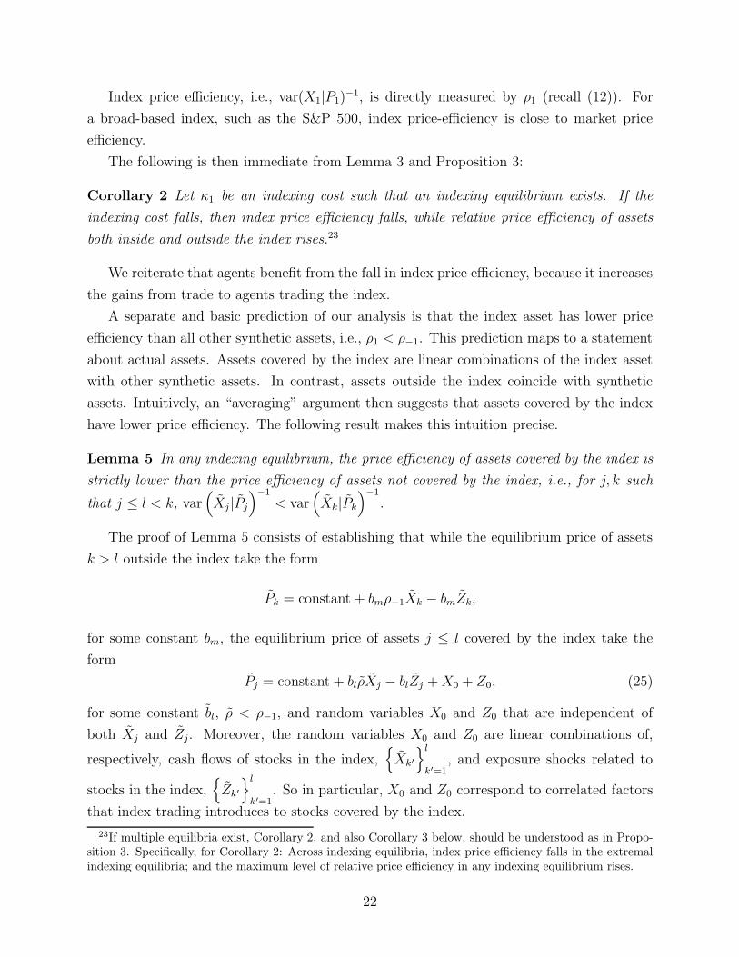
Corollary 2 Let κ1 be an indexing cost such that an indexing equilibrium exists. If the

indexing cost falls, then index price efficiency falls, while relative price efficiency of assets

both inside and outside the index rises.23

We reiterate that agents benefit from the fall in index price efficiency, because it increases

the gains from trade to agents trading the index.

A separate and basic prediction of our analysis is that the index asset has lower price

efficiency than all other synthetic assets, i.e., ρ1 < ρ−1. This prediction maps to a statement

about actual assets. Assets covered by the index are linear combinations of the index asset

with other synthetic assets. In contrast, assets outside the index coincide with synthetic

assets. Intuitively, an “averaging” argument then suggests that assets covered by the index

have lower price efficiency. The following result makes this intuition precise.

Lemma 5 In any indexing equilibrium, the price efficiency of assets covered by the index is

strictly lower than the price efficiency of assets not covered by the index, i.e., for j, k such

that j ≤ l < k, var(

Xj |Pj

)−1

< var(

Xk|Pk

)−1

.

The proof of Lemma 5 consists of establishing that while the equilibrium price of assets

k > l outside the index take the form

Pk = constant + bmρ−1Xk − bmZk,

for some constant bm, the equilibrium price of assets j ≤ l covered by the index take the

form

Pj = constant + blρXj − blZj +X0 + Z0, (25)

for some constant bl, ρ < ρ−1, and random variables X0 and Z0 that are independent of

both Xj and Zj. Moreover, the random variables X0 and Z0 are linear combinations of,

respectively, cash flows of stocks in the index,{

Xk′

}l

k′=1, and exposure shocks related to

stocks in the index,{

Zk′

}l

k′=1. So in particular, X0 and Z0 correspond to correlated factors

that index trading introduces to stocks covered by the index.

23If multiple equilibria exist, Corollary 2, and also Corollary 3 below, should be understood as in Propo-sition 3. Specifically, for Corollary 2: Across indexing equilibria, index price efficiency falls in the extremalindexing equilibria; and the maximum level of relative price efficiency in any indexing equilibrium rises.

22

As discussed in the introduction, one might have conjectured that the fall in the price

efficiency of the index associated with lower indexing costs would make indexing less attrac-

tive for uninformed investors, thereby generating a countervailing force. Instead, our analysis

shows that the entry of uninformed investors is self-reinforcing: as more such investors enter,

and price efficiency drops, indexing becomes more attractive rather than less, attracting still

more uninformed investors.

Conversely, one might have conjectured that the rise in relative price efficiency of assets

covered by the index would make individual trades more attractive. Again, this is not the

case: this increase makes trading individual assets less attractive for uninformed investors,

and so is again self-reinforcing.

4.3 Indexing and expected utilities

As the cost κ1 of indexing falls, the expected utility of indexing agents increases, reflecting

both the lower cost, and also the lower price efficiency of the index asset. In contrast, the

expected utility of fully participating agents is subject to conflicting forces. On the one

hand, fully participating agents benefit from the lower price efficiency of the index asset. On

the other hand, they are harmed by the higher price efficiency of other assets.

Combining:

Corollary 3 Let κ1 be an indexing cost such that an indexing equilibrium exists. If the

indexing cost falls, the expected utility of indexing agents increases. For agents who fully

participate, the share of trading gains stemming from trading the index asset increase.

4.4 Indexing, reversals, and informed trading

A direct implication of market-clearing (4) and agents’ trading decisions (11) is that

1

γE [X1 − P1|P1]

1

n1

∫ n1

0

1

var (X1|yi1, ei1, P1)= S1 + E [Z1|P1] , (26)

with analogous identities for other assets. Moreover, from Lemma A-7, we know E [Z1|P1] is

decreasing in P1, i.e., prices and exposure shocks are negatively correlated. Consequently, our

framework naturally generates a reversal pattern in prices, with high prices today associated

with lower expected returns.24

24Consequently, if an investor observes a low price for an asset, and has no exposure to economic shocks,he should take a long position in the asset, since its conditional expected return is high. That is, an investorcan profit from buying “value” stocks. Although this point is often overlooked, it is nonetheless a standardimplication of models of the type we consider here (see, e.g., Biais, Bossaerts, and Spatt, 2010).

23

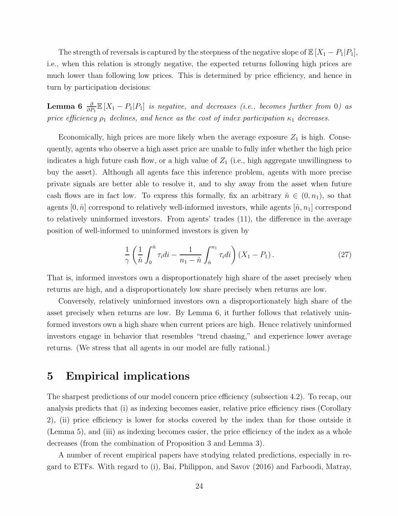
The strength of reversals is captured by the steepness of the negative slope of E [X1 − P1|P1],

i.e., when this relation is strongly negative, the expected returns following high prices are

much lower than following low prices. This is determined by price efficiency, and hence in

turn by participation decisions:

Lemma 6 ∂∂P1

E [X1 − P1|P1] is negative, and decreases (i.e., becomes further from 0) as

price efficiency ρ1 declines, and hence as the cost of index participation κ1 decreases.

Economically, high prices are more likely when the average exposure Z1 is high. Conse-

quently, agents who observe a high asset price are unable to fully infer whether the high price

indicates a high future cash flow, or a high value of Z1 (i.e., high aggregate unwillingness to

buy the asset). Although all agents face this inference problem, agents with more precise

private signals are better able to resolve it, and to shy away from the asset when future

cash flows are in fact low. To express this formally, fix an arbitrary n ∈ (0, n1), so that

agents [0, n] correspond to relatively well-informed investors, while agents [n, n1] correspond

to relatively uninformed investors. From agents’ trades (11), the difference in the average

position of well-informed to uninformed investors is given by

1

γ

(

1

n

∫ n

0

τidi−1

n1 − n

∫ n1

n

τidi

)

(X1 − P1) . (27)

That is, informed investors own a disproportionately high share of the asset precisely when

returns are high, and a disproportionately low share precisely when returns are low.

Conversely, relatively uninformed investors own a disproportionately high share of the

asset precisely when returns are low. By Lemma 6, it further follows that relatively unin-

formed investors own a high share when current prices are high. Hence relatively uninformed

investors engage in behavior that resembles “trend chasing,” and experience lower average

returns. (We stress that all agents in our model are fully rational.)

5 Empirical implications

The sharpest predictions of our model concern price efficiency (subsection 4.2). To recap, our

analysis predicts that (i) as indexing becomes easier, relative price efficiency rises (Corollary

2), (ii) price efficiency is lower for stocks covered by the index than for those outside it

(Lemma 5), and (iii) as indexing becomes easier, the price efficiency of the index as a whole

decreases (from the combination of Proposition 3 and Lemma 3).

A number of recent empirical papers have studying related predictions, especially in re-

gard to ETFs. With regard to (i), Bai, Philippon, and Savov (2016) and Farboodi, Matray,

24

and Veldkamp (2018) find that relative price efficiency has trended upwards over approxi-

mately the last 50 years, over broadly the same time period in which indexing has become

more prevalent. Over a more recent period, Glosten, Nallareddy, and Zou (forthcoming)

document that relative price efficiency increases precisely as ETF ownership of the under-

lying shares increases.25Antoniou et al. (2019) show that an increase in ETF ownership is

associated with a strengthening of the link between a firm’s investment and its own stock

price; since the empirical analysis includes time fixed effects, this suggests that managers

believe that increased ETF ownership increases relative price efficiency, consistent with our

model.26

With regard to (ii), Coles, Heath, and Ringgenberg (2020) and Bennett, Stulz, and Wang

(2020) find that inclusion in the Russell 2000 and SP 500 indices, respectively, is associated

with a decline in price efficiency. Farboodi, Matray, and Veldkamp (2018) show that for

stocks that have been included in the S&P 500 at some point in time, price efficiency is lower

during periods in which they are included. Qin and Singal (2015) find that price efficiency

of a stock decreases in a measure of its “indexed ownership.” Ben-David, Franzoni, and

Moussawi (2018) document that ETF ownership increases stock volatility, consistent with

the hypothesis that ETFs enable “liquidity shocks [to] propagate.” Also consistent with our

analysis, they provide evidence that the increase in volatility is not due to increased price

efficiency. Similarly, Brogaard, Ringgenberg, and Sovich (forthcoming) show that firms

that use commodities covered by leading commodity indices make less efficient production

decisions than firms that use commodities outside these indices.

While prediction (iii) is harder to directly test, a closely related prediction is that, as

indexing increases, informed trading profits will stem increasingly from “timing” strategies

based on the entire index, rather than individual asset trades. (See Corollary 3, with the

caveat that expected utilities are distinct objects from expected profits.) There is at least

some empirical evidence supporting this prediction. AQR document that the correlation

between hedge fund returns and market returns has risen from 0.6 to 0.9 over the last two

25We also note that Farboodi, Matray, and Veldkamp (2018) additionally show that relative price efficiencyhas declined for stocks outside the S&P 500, a finding that is inconsistent with our model. Among otherthings, these authors emphasize the importance of accounting for changes in firm size, which is outside thescope of our analysis. Israeli, Lee, and Sridharan (2017) estimate similar empirical specifications to Glosten,Nallareddy, and Zou (forthcoming), but use lagged changes in ETF ownership, and show that these areassociated with decreases rather than increases in relative price efficiency.

26Section 7 below formally incorporates managerial learning from prices. Antoniou et al. (2019) furtherdecompose stock prices into systematic and idiosyncratic components, where the systematic componentcaptures differences explained by time and industry effects. They find that increased ETF ownership hasa greater effect on the relation between investment and the systematic component of cash flows. This isconsistent with an asset k in our model corresponding to an industry as opposed to an individual firm.

25

decades.27 Related, Stambaugh (2014) documents a decline in asset-selection strategies by

active mutual funds over the same period. Also related, and using data since 2000, Gerakos,

Linnainmaa, and Morse (2019) show that a significant fraction of returns generated by active

mutual funds stem from market timing strategies.

Our model can also be used to study the effect of index inclusion on return variances and

covariances. For example, and as one would expect, index inclusion introduces a common

component to stock prices; see discussion immediately following Lemma 6. This is consistent

with evidence in Vijh (1994), Barberis, Shleifer, and Wurgler (2005), Greenwood (2008),

and Bennett, Stulz, and Wang (2020); and related, Da and Shive (2018) and Leippold, Su,

and Ziegler (2016) present evidence that individual stock correlations have risen with ETF

ownership. As noted, Ben-David, Franzoni, and Moussawi (2018) present evidence that ETF

ownership raises the volatility of individual stock prices.

The analysis in subsection 4.4 predicts that relatively uninformed ownership of an asset

increases when prices are high, and that this is followed by low subsequent returns. This

is consistent with the empirical evidence in Ben-Rephael, Kandel, and Wohl (2012) for

the market as a whole (i.e., the index asset), and in Jiang, Verbeek, and Wan (2017) and

Grinblatt et al. (2020) in the cross-section.28 Furthermore, Lemma 6 is consistent with the

empirical findings of Baltussen, van Bekkum, and Da (2019), who use international data to

document that negative serial correlation in index returns is associated with greater indexing,

and with Ben-David, Franzoni, and Moussawi (2018) who find that “ETF ownership increases

the negative autocorrelation in stock prices.”

Finally, it is worth noting that our model does not generate a price premium for index

inclusion, contrary to at least some empirical evidence. The reason is that changes in par-

ticipation in our model are always accompanied by changes in the supply of the asset being

traded, since we assume all agents have the same initial endowment.29 Because of this, index

inclusion affects prices only via its effect on price efficiency; and since price efficiency falls,

this leads to a fall in prices. In contrast, if one were to relax the assumption of equal initial

27See “Hedge fund correlation risk alarms investors,” Financial Times, June 29th, 2014.28Less directly, this prediction is also consistent with the finding in Kacperczyk, Van Nieuwerburgh, and

Veldkamp (2014) that the fraction of mutual fund returns stemming from timing strategies is greater inrecessions. Specifically, in our setting informed investors should shift into the index when index pricesare low, and out of the index when index prices are high. To the extent to which the second half ofthis strategy is constrained by difficulties shorting the index, this generates the findings of Kacperczyk,Van Nieuwerburgh, and Veldkamp (2014). (We should also note that the same authors suggest a distinctexplanation in Kacperczyk, Van Nieuwerburgh, and Veldkamp (2016).)

29Recall, in turn, that we use this assumption in the proof of Proposition 1. The empirical evidence onthe effects of index inclusion is mixed; while older studies found positive price reactions, Bennett, Stulz, andWang (2020) find that in more recent data “the positive announcement effect on the stock price of [S&P500] index inclusion has disappeared.”

26

endowments, the effect on prices would be determined by the relative strength of changes in

price efficiency and changes in the aggregate risk-sharing capacity of participating agents.

In general, we emphasize again that our model’s primary empirical predictions operate via

price efficiency.

6 Direct versus equilibrium effects

The consequences of a decline in indexing costs stem from a combination of direct effects

(e.g., more people index because of lower costs, and price efficiency is lower because the new

people indexing are relatively uninformed) and equilibrium effects (e.g., lower price efficiency

of the index further increases the attractiveness of indexing). In this section, we discuss the

relative contributions of the direct and equilibrium effects.

6.1 Spillover effects of changes in informedness

We have focused on the comparative static associated with indexing costs κ1. Naturally,

however, there are other interesting questions that one could pursue using our framework.

Here, we examine the consequences of an increase in the informedness of the most informed

agents in the economy. The idea that the most informed agents have grown more informed

has been suggested by a number of authors (e.g., Glode, Green, and Lowery (2012), Fishman

and Parker (2015), Bolton, Santos, and Scheinkman (2016); closely related is the idea that

“big data” and data processing have grown in importance, e.g., Farboodi, Matray, and

Veldkamp (2018)). This exercise has the virtue of highlighting the role of equilibrium effects;

in particular, since participation costs are unchanged, there is no direct effect.

Concretely, we consider a parameterization of our economy in which an indexing equilib-

rium (n1, n−1) exists, with n−1 > 0 so that some agents fully participate and actively trade

assets other than the index. We then consider the consequences of increasing the precision

of signals of the most informed agents [0, n], where n < n−1.

This increase in the informedness of the most informed agents increases the price efficiency

of both index and non-index assets. Consequently, fewer agents fully participate, and fewer

agents participate in financial markets (either fully or via indexing). In other words, even

though an increase in signal precisions makes prices more informativeness, it makes financial

markets less beneficial for agents. Hence our framework formalizes the channel via which in

increase in sophistication of the financial specialists places “ordinary” uninformed investors

at an increasing disadvantage (see references above). It also speaks to the older question of

whether insider trading is socially costly (e.g., Fishman and Hagerty (1992), Khanna, Slezak,

27

and Bradley (1994)).

6.2 Numerical decomposition of direct versus equilibrium effects

We now return to our main comparative static of considering a drop in indexing costs κ1.

We again starting from an indexing equilibrium (n1, n−1) with n−1 > 0, and associated

equilibrium price efficiency levels ρ1 and ρ−1. A fall in κ1 leads to a new equilibrium with

more total participation (n1 higher) and less full participation (n−1 lower); see Proposition 3.

This equilibrium effect can be decomposed into the direct effect associated with the change in

cost κ1, which we define as agents’ participation decisions under the new costs, but assuming

that price efficiency remains fixed at the original level (ρ1, ρ−1); and the remaining change,

which by definition is the equilibrium effect.

We illustrate the relative size of these effects via numerical simulation. We emphasize

that we view the simulation as being for illustrative purposes only; a realistic calibration of

our model is beyond the scope of this paper, and in any case, for calibration one would want

to consider a dynamic version of our model. We detail the parameters used for the numerical

simulation in Appendix D.

As a first step, Figure 6.2 shows the equilibria of our economy. The lefthand panel plots

the following: for a candidate fraction of agents who trade the index asset (the horizontal

axis), find the price efficiency of the index asset (Lemma 3), and then find the fraction

of agents who prefer indexing to autarchy. Stable equilibria correspond to points where

this function crosses the 45o line from above. The middle and righthand plots show the

corresponding functions for the choice of full participation versus indexing, and the choice

of full participation versus autarchy.

One point that is immediately apparent from Figure 6.2 is that the strategic complemen-

tarity effect in our model is strong, and multiple equilibria exist. This arises in all numerical

simulations that we examined. Specifically, there are four stable equilibria: No-one partic-

ipates (n1 = n−1 = 0); everyone fully participates (n1 = n−1 = 1); n1 = 62.14% index and

no-one fully participates (n−1 = 0); and n1 = 62.14% participate with n−1 = 25.65% fully

participating, so that 36.49% index. We focus on the last of these equilibria. (We do not see

any good theoretical argument for selecting among these equilibria; and the one we focus

on matches the empirical fact that some agents trade actively, some index, and some do not

participate.)

Next, we consider a small 1% decrease in the cost of indexing κ1. Table 6.2 displays the

results of the decomposition described above. The decomposition shows that the direct and

equilibrium effects are of the same order of magnitude, and that both are sizable (the total

28

0 50 100

0

10

20

30

40

50

60

70

80

90

100Index vs autarchy

0 50 100

0

10

20

30

40

50

60

70

80

90

100Full vs index

0 50 100

0

10

20

30

40

50

60

70

80

90

100Full vs autarchy

Figure 1: Equilibrium participation

29

Values under initial costs Total change Change due to Change due todirect effect equilibrium effect

n1 62.14% +1.3% +0.77% +0.53%n−1 25.65% −0.52% −0.30% −0.22%

Table 1: Decomposition into direct and equiulibrium effects. Changes are in percentagepoints.

elasticity with respect to cost changes is approximately 2).

7 Indexing and firm performance: Price efficiency and

feedback effects

The rise of index investing has generated a variety of concerns about the effect of indexing

on firm performance, including, for example, the fears that indexing investors will spend

less effort on firm governance, or that indexing results in extensive common ownership,

leading to reduced competition between firms, thereby reducing consumer surplus.30 We

have deliberately focused our analysis on indexing’s effects in an endowment economy, in

order to clearly delineate what we believe is an important channel.

The central economic force in our model is that indexing costs affect participation, which

affects price efficiency, which in turn affect participation. As such, the link between indexing

and firm performance that our analysis can best speak to is the possible effect of prices on

firms’ real decisions, a channel often referred to as the “feedback effect” (see Bond, Goldstein,

and Edmans (2012) for a survey). To this end, in this section we extend our baseline model

to allow for feedback effects. The extension is rich enough to embody two key effects, yet

simple enough to remain tractable.31

30For a discussion of the first point, along with some evidence against, see for example Appel, Gormley,and Keim (2016). For a discussion of the second point, see, for example, Azar, Schmalz, and Tecu (2018)and Schmalz (2018).

31A standard tractability hurdle in feedback models is to make sure that the distribution of the endogenouscash flow is such that agent’s portfolio decisions generate prices that allow for a tractable treatment ofagents’ updating from prices. Papers such as Sockin and Xiong (2015), Bond and Goldstein (2015), Sockin(2018), and Goldstein and Yang (2019) all contain competitive models of financial markets with asymmetricinformation in which economic agents extract information from financial prices and use this information toaffect firm cash flows. On top of this standard hurdle, we also need to ensure that it remains feasible tocharacterize participation decisions (Proposition 2, in turn building on Proposition 1). The issue here is thatCorollary 1—which, as we have noted, is key to characterizing expected utilities and hence participation—does not generalize to settings with feedback effects. The reason that our analysis in this section is nonethelesstractable is that it is one in which the feedback effects shift index cash flows only by a constant; the effectson long-short porfolios (e.g., synthetic asset 2) are more complicated, but these assets are in zero net supply,

30

7.1 Extended model

There are two assets covered by the index, m = l = 2. (These two assets can be interpreted

as covering broad sectors of the economy.) We denote by Vk the cash flow that is produced

by each of assets k = 1, 2. This cash flow is determined by a mixture of exogenous and

endogenous factors. Specifically, let η ≥ 0 be a constant; the endogenous components of

cash flows, which we denote by Ξ1 and Ξ2, are determined by

Ξ1 = argmaxξ

E

[

ξ − exp(

ξ − ηX1 + ηX2

)

|P1, P2

]

(28)

Ξ2 = argmaxξ

E

[

ξ − exp(

ξ − ηX2 + ηX1

)

|P1, P2

]

, (29)

where Xk continues to denote an exogenous and randomly distributed random variable; and

the total cash flow of each asset k = 1, 2 is

Vk = Xk + Ξk.

In words: Xk is an exogenous shock to the business environment of firm (or sector) k, and Ξk

is the effect of the actions of firm k’s executives on cash flows. These actions—for example,

firm expansion, or the consumption of private benefits—are chosen prior to the realization

of exogenous business environment shocks Xk; but the realized net benefit or cost of these

actions to executives depends on the realization of the business environment. In particular,

expansion of firm 1 has a lower marginal cost for firm 1’s executives when firm 1’s business

environment is more favorable, or when firm 2’s business environment is more favorable.32

Feedback effects arise in this setting because firms’ executives seek to learn about the

future business environment, X1, X2, from the financial asset prices P1, P2. Note that by

setting the parameter η to 0, executives’ decisions are independent of expectations about

X1, X2, and hence independent of prices P1, P2, so that this framework nests our baseline

model of exogenous cash flows as a special case.

Finally, an agent’s non-financial income continues to be given by (1), and in particular,

is unaffected by firm’s endogenous decisions.

7.2 Endogenous cash flows

It is straightforward to show that there is an equilibrium in which prices are linear functions

of the exogenous business environment shocks X1, X2 and the aggregate exposure shocks Z1,

and for zero net supply assets Corollary 1 trivially generalizes.32The use of the exponential function as the cost function in (28) and (29) is not essential; see Bond and

Goldstein (2015).

31

Z2. Given this, executives’ conditional expectations of X1, X2 are normal, and (28), (29)

rewrite as

Ξk = argmaxξ

(

ξ − exp

(

ξ − ηE[

Xk − X−k|P1, P2

]

+1

2η2var

(

Xk − X−k|P1, P2

)

))

,

where X−k denotes the business environment j 6= k. Hence

Ξk = ηE[

Xk − X−k|P1, P2

]

− 1

2η2var

(

Xk − X−k|P1, P2

)

.

We again analyze the economy in terms of synthetic assets, defined exactly as before. Since

there are two underlying assets there are two synthetic assets, which we refer to as the index

and spread asset, having cash flows V1 = X1+Ξ1 and V2 = X2+Ξ2, where Ξ1 and Ξ2 denote

the endogenous components of the synthetic asset cash flows:

Ξ1 = −η2var(

X1 − X2|P1, P2

)

= −2η2var (X2|P2) (30)

Ξ2 = 2ηE[

X1 − X2|P1, P2

]

= 23

2 ηE [X2|P2] . (31)

Note that the price P1 of the index asset contains no information about the difference in

business environments X2, as reflected in (30) and (31).

That is: Feedback affects the index cash flow by a term that is constant in equilibrium,

−2η2var (X2|P2). Moreover, this term captures the intuitive idea that cash flows are higher

when price efficiency is greater, so that var (X2|P2) is lower. The price efficiency that matters

is the price efficiency of the non-index asset 2, i.e., relative price efficiency.

In contrast, the unconditional mean of spread asset’s cash flow V2 is 0, regardless of

either the strength of feedback η or of price efficiency. Instead, feedback in the spread asset

implies that its cash flow responds to the price realization, increasing the volatility of the

spread asset’s cash flow. This effect is stronger when price efficiency is greater and hence

the conditional expectation E [X2|P2] is more volatile.

7.3 Equilibrium

The endogenous components of the cash flows, Ξk, are deterministic functions of prices Pk.

(One can see this directly from (28), (29), without appealing to the specific expressions in

(30), (31).) Given this, it is convenient to analyze the economy in terms of the prices of

assets that pay only the exogenous cash flows Vk − Ξk = Xk. We denote the price of these

32

assets by PXk , and note that, precisely because Ξk is deterministic given prices,

PXk = Pk − Ξk.

Hence agent i’s terminal wealth given trades θi is

Wi =2∑

k=1

θik(

Xk − PXk

)

+ Sk (Xk + Ξk) + (Zk + uik)Xk

=2∑

k=1

θik(

Xk − PXk

)

+ eikXk + SkΞk, (32)

where per capita endowments are S1 =√2S and S2 = 0 for the index and spread assets.

An immediate implication of these observations is that, given participation decisions,

equilibrium price efficiency is exactly as before (Lemma 3).

The combination of (30), (31) and (32) means that participation decisions in the feedback

economy are no harder to analyze than in our baseline case without feedback (η = 0). For

the index asset, feedback adds a cash flow component Ξ1 that is constant in equilibrium,

and is received both by agents who trade the index asset and those who do not participate

(θi1 = 0) and simply hold their original endowment. Consequently, feedback has no effect

on participation decisions for the index asset.

For the spread asset, feedback adds a cash flow component Ξ2 that fluctuates with the

price of the spread asset P2. But because the spread asset is in zero supply, S2 = 0, this

endogenous component does not affect participation decisions, as (32) makes clear.

7.4 Effects of falling costs of indexing

With the equilibrium characterization in hand, we revisit our central topic, viz, the equilib-

rium effects of a falling cost of indexing. As noted, price efficiency and participation decisions

are unchanged from the baseline case. Nonetheless, feedback introduces two new effects.

First, as indexing costs κ1 fall, the increase in the price efficiency of the spread asset

reduces uncertainty about business conditions X1 and X2 inducing executives to work harder

(or consume fewer private benefits), thereby increasing the cash flow of firms, and hence of

the index asset. This creates an additional welfare benefit for all agents in the economy who

are endowed with a long position in the underlying assets (in our model, this is all agents).

Second, as indexing costs κ1 fall, the increase in the price efficiency of the spread asset

increases the sensitivity of cash flows to the price of the spread asset P2, consistent with

33

the empirical findings in Antoniou et al. (2019);33 and since the equilibrium price PX2 of the

exogenous part of cash flows coincides with the baseline case, it follows that cash flows grow

more volatile. Nonetheless, this increase in cash flow volatility leaves welfare unchanged,

since returns Vk − Pk = Xk − PXk are unaffected, and agents have no initial endowment of

the spread asset (see (32)).34

8 Discussion

8.1 Multiple indices

So far, we have focused on the case of a single index, which we have typically interpreted as a

broad-based market index such as the S&P500. In reality of course, a large number of indices

co-exist, and investment vehicles such as ETFs are increasingly available on this assortment

of indices (see, for example, Lettau and Madhaven (2018) and Easley et al. (2020)).

We can straightforwardly extend our analysis to cover multiple indices, at least when the

indices are orthogonal to each other. To fix ideas, we consider here the case of two indices:

the first a broad-based market index, corresponding to synthetic asset 1; and the second an

index corresponding to the long-short positions associated with synthetic asset 2, which by

construction is uncorrelated with synthetic asset 1. For example, the second index might be

an index tracking the value factor, which is constructed as a long-short portfolio, and which

indeed has low correlation with the overall market. Moreover, there are a number of ETFs

that track the value factor.

The participation cost of participating via the market index is κ1, and the participation

cost of participating via the value factor is κ2. Hence an agent now has two additional

participation options—participation via just the value factor, and participation via the com-

bination of the market index and value factor—along with the three possibilities considered

so far (no participation, market index, full participation).

A fall in the cost κ2 of participating via the value factor has effects that are analogous

to those analyzed so far. As this cost falls, more agents trade the value factor, decreasing

the price efficiency of the value factor, thereby further increasing the attractiveness of the

value factor. In a typical case, the increased attractiveness of participation via value factor

strategies reduces the number of agents who fully participate in financial markets, increasing

33Here, we are viewing empirically-measured investment as a proxy for the decisions Ξk; our analysispredicts that the sensitivity of the relative decision Ξ2 to the price difference P2 rises with indexing.

34As noted from the outset, the particular framework we have analyzed is special in significant respects,and other specifications of feedback would potentially yield different implications for a reduction in indexingcosts. But the framework we use has the advantages of being highly tractable, and allowing us to highlighttwo specific consequences of extending our model to allow prices to affect cash flows.

34

the price efficiency of assets not covered by either the market index of the value factor, and

also of synthetic assets other than those corresponding to the market index and value factor,

and that may correspond to other factors.

8.2 Intensive margin of information acquisition

While the participation decision in our model can be thought of as an information acquisition

decision on the extensive margin, we have abstracted away from the intensive margin of

agents’ information acquisition efforts. Here, we briefly consider an extension that features

an intensive margin. For simplicity, we focus on the case of two assets, l = m = 2, so that

the synthetic assets are simply an index asset and a spread asset.

Suppose now that, instead of being exogenously endowed with informative signals about

cash flows yik, agents spend resources to collect information. Specifically, for constants ci > 0

and η, in order to collect signals about the index asset 1 and spread asset 2 with precisions

τi1 and τi2, respectively, agent i incurs a cost

ci(

τ 2i1 + τ 2i2 + ητi1τi2)

. (33)

In words: Agent i faces convex costs of increasing precision, and these costs vary across

agents. We assume that agents choose precisions at the same time that they make partici-

pation decisions.

The cost specification (33) says that agents collect two types of information: information

about market aggregates, yi1, and information about relative cash flows, yi2. We believe this

assumption is realistic; it also has the important advantage of allowing us to continue to

analyze the economy in terms of the synthetic index and spread assets.35

The parameter η in (33) captures the multitasking dimension of information acquisition.

In particular, if η > 0, then an increase in the precision of the signal about X1 increases the

the marginal cost of precision about X2, and vice versa.

Absent multitasking considerations (i.e., η = 0), the above model generates qualitatively

the same implications as our main model. Specifically, a fall in the cost of indexing κ1 has the

direct effect of decreasing participation in the spread asset and increasing participation in

the index asset. If precision decisions are artificially held fixed, these changes in participation

decrease price efficiency in the index asset and increase price efficiency in the spread asset.

Consequently, in equilibrium agents who trade the spread asset reduce the precisions of their

35In contrast, if we instead assumed that agents can choose precisions of signals about the underlying cashflows X1 and X2, then the change-of-basis to synthetic assets is much less useful. In a different context,Van Nieuwerburgh and Veldkamp (2010) establish conditions under which investors would indeed want tospecialize and focus their information acquisition efforts on a small number of assets.

35

spread asset signals, while agents who trade the index asset increase the precision of their

index asset signals. These endogenous changes in precision dampen the effect of the fall in

indexing costs, but do not qualitatively change any of the predictions, since the net effect is

still that equilibrium price efficiency rises in the spread asset and falls in the index asset.36

Multitasking considerations—and specifically, the case in which precision of one signal

increases the marginal cost of the other signal, i.e., η > 0—introduce an additional effect,

as follows. To isolate the effect in a transparent way, we consider the case in which κ1 is

sufficiently low that all agents trade the index asset, and a strict subset of agents trade

spread asset. In this case, a further reduction in κ1 reduces the number of agents trading the

spread asset; but does not affect the number of agents trading the index asset, since everyone

already trades it. So if precision decisions are artificially held fixed, the price efficiency of

the spread asset increases, while the price efficiency of the index asset is unchanged.

The new effect introduced by multitasking is that agents respond by increasing the preci-

sion of signals about the index asset, as follows. Agents who trade the spread asset respond

to the increase in its price efficiency by reducing the precision of signals about the spread as-

set, and—because of multitasking—increasing the precision of signals about the index asset.

Agents who previously traded the spread asset, but no longer do so after the fall in indexing

costs, likewise respond by increasing the precision of signals about the index asset, again for

multitasking reasons. Consequently, and different from our baseline model, price efficiency of

the index asset rises rather than falls. In this case, the fall in the cost of indexing generates

indirect effects that reduce the benefits of trading the index asset—though, of course, the

fall in indexing costs still carries a direct benefit.

As we noted, this multitasking effect is starkest in the case in which a fall in indexing

costs does not increase the number of agents trading the index asset. The case in which both

effects operate is more complicated, and the net effect is a quantitative question.

8.3 Revisiting the link between participation and price efficiency

The substantive implications of our analysis are all contingent on Lemma 3’s implication that

the price efficiency of an asset is decreasing in the level of participation in that asset. Recall

that this implication arises because the marginal new participating agent is less informed

than the average participating agent, but has the same non-informational trading motives.

Consequently, the marginal new participating agent adds proportionately more “noise” than

information to the market. Moreover, the empirical evidence surveyed in Section 5 provides

36This is straightforward to see. For example, suppose to the contrary that price efficiency rose in theindex asset. Then agents would decrease the precision of their signals, implying that price efficiency mustfall, a contradiction.

36

at least some support for the idea that price efficiency is decreasing participation.

Nonetheless, it is important to acknowledge that there are plausible economic forces that

would predict that price efficiency is instead increasing in participation:

Heterogenous risk aversion: If agents have differing levels of risk-aversion, γi, it is

straightforward to show that equilibrium price efficiency of asset k is given by the smaller

root of the quadraticρ2kτu|Nk|

∫

Nk

1

γidi− ρk +

1

|Nk|

∫

Nk

τiγidi = 0, (34)

where Nk is the set of agents participating in asset k. Consequently, a sufficient condition

Lemma 3’s conclusion that price efficiency is decreasing in participation to hold is that both1

|Nk|∫

Nk

1γidi and 1

|Nk|∫

Nk

τiγidi decrease in participation. Similarly, a sufficient condition for

price efficiency to increase in participation is that both 1|Nk|

∫

Nk

1γidi and 1

|Nk|∫

Nk

τiγidi increase

in participation.

In particular, if the agents differ only risk aversion levels, while having the same signal

precisions, then price efficiency is increasing in participation if the most risk-averse agents

gain most from participation. While, unfortunately, participation decisions are much harder

to evaluate analytically when risk aversion is heterogeneous, it is intuitive that participa-

tion gains are indeed increasing in risk aversion, and numerical simulations support this

intuition.37More generally, our analysis suggests that price efficiency is decreasing in partic-

ipation if the main source of heterogeneity among agents is differing signal precisions; but

increasing in participation if instead the main source of heterogeneity is differing levels of

risk aversion.

Quadratic trading costs in place of fixed participation costs: Our main model assumes

that agents pay fixed costs (κ and κ1) to participate in financial markets. An alternative

modeling approach would be to instead assume that agents incur costs at the time of trading.

To fix ideas, we consider here the highly tractable case in which trading costs take the form12κθ2ik, for some constant κ > 0, which is potentially smaller for trades of the index asset.38

Naturally, transaction costs reduce trade sizes, with (11) generalizing to

θik =E [Xk|yik, eik, Pk]− Pk − eikγvar (Xk|yik, eik, Pk)

γvar (Xk|yik, eik, Pk) + κ.

37See online appendix for expressions used in the numerical calculation. The main impediment to an ana-

lytical evaluation of participation is that the generalization of Corollary 1 delivers E [X − P ] = Scov(X−P,X)1

|N|

∫N

1

γidi

;

it then follows that the substitution of Corollary 1 in the proof of Proposition 1 is useful only for an agentwhose risk aversion γi matches the harmonic mean of participating agents.

38In an economy in which agents can observe the number of agents with a given signal who buy (re-spectively, sell) the asset, Davila and Parlatore (forthcoming) obtain results for linear and fixed transactioncosts.

37

Under this specification of costs, all agents participate in all markets, and costs affect the

intensive rather than extensive margin of participation. The relation between price efficiency

and the magnitude of the transaction cost parameter κ depends on relative effect of the

transaction cost on trade sensitivity to cash flow signals yik and exposure shocks eik, along

with how this relative sensitivity varies across agents with differing signal precisions.

Davila and Parlatore (forthcoming) analyze exactly this question in a closely related

economy, and find that the relation depends on the specific form of heterogeneity across

agents. In particular, they examine a model in which agents have heterogeneous prior be-

liefs about cash flows,39 and also observe subsequent signals of cash flows. They find that

price efficiency is decreasing in the transaction cost parameter if agents differ in their signal

precisions; but is increasing if instead agents differ in the accuracy of their prior beliefs.40

9 Conclusion

We develop a benchmark model to study the equilibrium consequences of indexing in a stan-

dard rational expectations setting (Grossman and Stiglitz (1980); Hellwig (1980); Diamond

and Verrecchia (1981)). Individuals must incur costs to participate in financial markets, and

these costs are lower for individuals who restrict themselves to indexing strategies. Individu-

als’ participation decisions exhibit strategic complementarity, and consequently, equilibrium

effects reinforce the direct consequences of declining costs of indexing. As indexing becomes

cheaper (1) indexing increases, while individual stock trading decreases; (2) aggregate price

efficiency falls, while relative price efficiency increases; (3) the welfare of relatively unin-

formed traders increases; (4) for well-informed traders, the share of trading gains stemming

from market timing increases, and the share of gains from stock selection decreases; (5)

market-wide reversals become more pronounced. We discuss empirical evidence for these

predictions.

39In Davila and Parlatore’s model, agents do not have exposure to non-financial cash flows (z + ui in ournotation) and instead trade because of heterogeneous prior beliefs.

40For completeness, in an online appendix we show that the former result relating to signal precisions holdsin our model also, at least for the case in which the population distribution of signal precisions is binary.

38

References

Admati, A. R. 1985. A noisy rational expectations equilibrium for multi-asset securitiesmarkets. Econometrica 53(3):629–57.

Admati, A. R., and P. Pfleiderer. 1997. Does it all add up? Benchmarks and the compensa-tion of active portfolio managers. The Journal of Business 70:323–50.

Antoniou, C., F. W. Li, X. Liu, A. Subrahmanyam, and C. Sun. 2019. The real effects ofexchange-traded funds. Working Paper .

Appel, I., T. Gormley, and D. Keim. 2016. Passive investors, not passive owners. Journal ofFinancial Economics 111–41.

Azar, J., M. Schmalz, and I. Tecu. 2018. Anticompetitive effects of common ownership.Journal of Finance 73:1513–65.

Bai, J., T. Philippon, and A. Savov. 2016. Have financial markets become more informative?Journal of Financial Economics 122:625–54.

Baltussen, G., S. van Bekkum, and Z. Da. 2019. Indexing and stock market serial dependencearound the world. Journal of Financial Economics 132:26–48.

Barberis, N., A. Shleifer, and J. Wurgler. 2005. Comovement. Journal of Financial Eco-nomics 75:283–317.

Baruch, S., and X. Zhang. 2018. Is index trading benign? Working Paper .

Basak, S., and A. Pavlova. 2013. Asset prices and institutional investors. American EconomicReview 103:1728–58.

Baumol, W. J. 1965. The stock market and economic efficiency. New York: FordhamUniversity Press.

Ben-David, I., F. Franzoni, and R. Moussawi. 2018. Do ETFs increase volatility? Journalof Finance 73:2471–535.

Ben-Rephael, A., S. Kandel, and A. Wohl. 2012. Measuring investor sentiment with mutualfund flows. Journal of Financial Economics 363–82.

Bennett, B., R. M. Stulz, and Z. Wang. 2020. Does joining the S&P 500 index hurt firms?Working Paper .

Bhattacharya, A., and M. O’Hara. 2018. Can ETFs increase market fragility? Effect ofinformation linkages in ETF markets. Working Paper .

Biais, B., P. Bossaerts, and C. Spatt. 2010. Equilibrium asset pricing and portfolio choiceunder asymmetric information. Review of Financial Studies 23:1503–43.

39

Bolton, P., T. Santos, and J. A. Scheinkman. 2016. Cream skimming in financial markets.Journal of Finance 71:709–36.

Bond, P., and I. Goldstein. 2015. Government intervention and information aggregation byprices. Journal of Finance 2777–812.

Bond, P., I. Goldstein, and A. Edmans. 2012. The real effects of financial markets. AnnualReview of Financial Economics 339–60.

Brogaard, J., M. C. Ringgenberg, and D. Sovich. forthcoming. The economic impact of indexinvesting. Review of Financial Studies .

Buffa, A. M., D. Vayanos, and P. Woolley. 2019. Asset management contracts and equilibriumprices. Working Paper .

Coles, J. L., D. Heath, and M. C. Ringgenberg. 2020. On index investing. Working Paper .

Cong, L. W., and D. X. Xu. 2019. Rise of factor investing: asset prices, informationalefficiency, and security design. Working Paper .

Da, Z., and S. Shive. 2018. Exchange traded funds and asset return correlations. EuropeanFinancial Management 24:136–68.

Davila, E., and C. Parlatore. forthcoming. Trading costs and informational efficiency. Journalof Finance .

Diamond, D. W. 1985. Optimal release of information by firms. Journal of Finance 40:1071–94.

Diamond, D. W., and R. E. Verrecchia. 1981. Information aggregation in a noisy rationalexpectations economy. Journal of Financial Economics 9:221–35.

Dow, J., and R. Rahi. 2003. Informed trading, investment, and welfare. Journal of Business439–54.

Easley, D., D. Michayluk, M. O’Hara, and T. J. Putniss. 2020. The active world of passiveinvesting. Working Paper .

Farboodi, M., A. Matray, and L. Veldkamp. 2018. Where has all the big data gone? WorkingPaper .

Fishman, M. J., and K. M. Hagerty. 1992. Insider trading and the efficiency of stock prices.RAND Journal of Economics 23:106–22.

Fishman, M. J., and J. A. Parker. 2015. Valuation, adverse selection, and market collapses.Review of Financial Studies 28:2575–607.

French, K. R. 2008. Presidential address: The cost of active investing. The Journal ofFinance 63:1537–73.

40

Ganguli, J., and L. Yang. 2009. Complementarities, multiplicity, and supply information.Journal of the European Economic Association 7(1):90–115.

Garcıa, D., and J. M. Vanden. 2009. Information acquisition and mutual funds. Journal ofEconomic Theory 144:1965–95.

Garleanu, N., and L. H. Pedersen. 2018. Efficiently inefficient markets for assets and assetmanagement. Journal of Finance 73:1663–712.

Gerakos, J., J. Linnainmaa, and A. Morse. 2019. Asset managers: Institutional performanceand factor exposures. Working Paper .

Glode, V., R. C. Green, and R. Lowery. 2012. Financial expertise as an arms race. Journalof Finance 67:1723–59.

Glosten, L., S. Nallareddy, and Y. Zou. forthcoming. ETF activity and informational effi-ciency of underlying securties. Management Science .

Goldstein, I., and L. Yang. 2019. Commodity financialization and information transmission.Working Paper .

Greenwood, R. 2008. Excess comovement of stock returns: Evidence from cross-sectionalvariation in nikkei 225 weights. Review of Financial Studies 21:1153–86.

Grinblatt, M., G. Jostova, L. Petrasek, and A. Philipov. 2020. Style and skill: Hedge funds,mutual funds, and momentum. Working Paper .

Grossman, S. J. 1976. On the efficiency of competitive stock markets where trades havediverse information. Journal of Finance 31(2):573–85.

Grossman, S. J., and J. E. Stiglitz. 1980. On the impossibility of informationally efficientmarkets. American Economic Review 70(3):393–408.

Hellwig, M. F. 1980. On the aggregation of information in competitive markets. Journal ofEconomic Theory 22:477–98.

Hirshleifer, J. 1971. The private and social value of information and the reward to inventiveactivity. The American Economic Review 61:561–74.

Israeli, D., C. Lee, and S. A. Sridharan. 2017. Is there a dark side to exchange traded funds?An information perspective. Review of Accounting Studies 1048–83.

Jiang, H., M. Verbeek, and Y. Wan. 2017. Information content when mutual funds deviatefrom benchmarks. Management Science 2038–53.

Kacperczyk, M., S. Van Nieuwerburgh, and L. Veldkamp. 2014. Time-varying fund managerskill. Journal of Finance 69.

———. 2016. A rational theory of mutual funds’ attention allocation. Econometrica 84.

41

Kawakami, K. 2017. Welfare consequences of information aggregation and optimal marketsize. American Economic Journal: Microeconomics 303–23.

Khanna, N., S. L. Slezak, and M. Bradley. 1994. Insider trading, outside search, and resourceallocation: why firms and society may disagree on insider trading restrictions. Review ofFinancial Studies 7:575–608.

Kurlat, P. 2019. The social value of financial expertise. American Economic Review 109:556–90.

Kurlat, P., and L. Veldkamp. 2015. Should we regulate financial information? Journal ofEconomic Theory 158:697–720.

Leippold, M., L. Su, and A. Ziegler. 2016. How index futures and ETFs affect stock returncorrelations. Working Paper .

Lettau, M., and A. Madhaven. 2018. Exchange-traded funds 101 for economists. Journal ofEconomic Perspectives 32:135–54.

Manzano, C., and X. Vives. 2011. Public and private learning from prices, strategic sub-stitutability and complementarity, and equilibrium multiplicity. Journal of MathematicalEconomics 47(3):346–69.

Marın, J. M., and R. Rahi. 1999. Speculative securities. Economic Theory 14:653–68.

Medrano, L. A., and X. Vives. 2004. Regulating insider trading when investment matters.Review of Finance 199–277.

Qin, N., and V. Singal. 2015. Indexing and stock price efficiency. Financial Management44:875–904.

Schlee, E. E. 2001. The value of information in efficient risk-sharing arrangements. AmericanEconomic Review 91:509–24.

Schmalz, M. 2018. Common-ownership concentration and corporate conduct. Annual Reviewof Financial Economics 10.

Sockin, M. 2018. Financial sector transparency and real investment. Working Paper .

Sockin, M., and W. Xiong. 2015. Informational frictions and commodity markets. Journalof Finance 70:2063–98.

Stambaugh, R. F. 2014. Presidential address: Investment noise and trends. The Journal ofFinance 69:1415–53.

Subrahmanyam, A. 1991. A theory of trading in stock index futures. Review of FinancialStudies 17–51.

Van Nieuwerburgh, S., and L. Veldkamp. 2010. Information acquisition and under- diversi-fication. Review of Economic Studies .

42

Verrecchia, R. E. 1982. Information acquisition in a noisy rational expectations economy.Econometrica 50(6):1415–30.

Vijh, A. M. 1994. S&P 500 trading strategies and stock betas. Review of Financial Studies7:215–51.

43

A Results omitted from main text

Note: Throughout the appendix, we frequently omit asset subscripts in order to enhance

notational transparency.

Lemma A-1 For any positive integers m and l ≤ m such that l is a power of 2, there

exists an m×m matrix A with the following properties: A is symmetric and invertible, with

A−1 = A (i.e., A is involutory); Ajk = 0 if j 6= k and either j > l or k > l; Ajk = 1 if

j = k > l; A1k = l−1

2 and |Ajk| = l−1

2 for all j, k ≤ l; for any j, j′ 6= j,∑m

k=1AjkAj′k = 0;

and∑l

k=1Ajk = 0 for j = 2, . . . , l.

Proof of Lemma A-1: We focus on cases l = m, since the generalization to l < m is

trivial. The proof is inductive: Given the existence of an m ×m matrix A with the stated

properties, we construct a 2m× 2m matrix B with the same properties. Specifically, define

B =1√2

(

A A

A −A

)

.

With the exception of the symmetry and inversion properties, it is straightforward to see

that B has the desired properties. To establish that B is involutory, simply note that

BB =1

2

(

A A

A −A

)(

A A

A −A

)

=1

2

(

AA + AA AA− AA

AA−AA AA + AA

)

=1

2

(

2Im 0m

0m 2Im

)

= I2m,

where Im denotes the m×m identity matrix and 0m denotes the m×m matrix in which all

entries are zero. To establish that B is symmetric, simply note that

B⊤ =1√2

(

A⊤ A⊤

A⊤ −A⊤

)

=1√2

(

A A

A −A

)

= B.

Finally, for the base case of m = 1, simply define A = (1). This completes the proof.

Lemma A-2 Let A be a matrix with the properties stated in Lemma A-1. Define synthetic

assets as paying off

Xk ≡m∑

j=1

AkjXj . (A-1)

The synthetic assets have the properties stated in the main text. Moreover, the price vectors

for fundamental and synthetic assets are related by P = AP and P = AP .

44

Proof of Lemma A-2: The properties of the synthetic assets all follow directly from the

properties of the matrix A. For the price vectors, the statement P = AP is immediate from

construction. Since A is involutory, it follows that AP = P .

Lemma A-3 Suppose X is a normally distributed random variable, and that an information

set F consists of a set of normally distributed random variables. Then the derivative of the

conditional expectation E [X|F ] with respect to a realization X of X is

∂

∂XE [X|F ] = 1− var (X|F)

var (X).

Proof of Lemma A-3: Let Σ22 be the variance matrix of the random variables in F ; and

Σ12 be the row vector of covariances between X and the random variables in F . The vector

of coefficients from the regressing each variable in F on X is Σ12

var(X). So by the properties of

multivariate normality,∂

∂XE [X|F ] = Σ12Σ

−122

Σ⊤12

var (X).

Also from multivariate normality,

var (X|F) = var (X)− Σ12Σ−122 Σ

⊤12.

Combining these two equations completes the proof.

Lemma A-4 Let ξ ∈ Rn be a normally distributed random vector with mean µ and variance-

covariance matrix Σ. Let b ∈ Rn be a given vector, and A ∈ R

n×n a symmetric matrix. If

I − 2ΣA is positive definite, then E[

exp(b⊤ξ + ξ⊤Aξ)]

is well defined, and given by:

E[

exp(

b⊤ξ + ξ⊤Aξ)]

= |I−2ΣA|−1/2 exp

(

b⊤µ+ µ⊤Aµ+1

2(b+ 2Aµ)⊤(I − 2ΣA)−1Σ(b+ 2Aµ)

)

.

(A-2)

Proof of Lemma A-4: Standard result.

Lemma A-5 In a linear equilibrium, ∂Pk

∂Zk

6= 0, and hence ρk is well-defined.

Proof of Lemma A-5: Differentiation of market clearing (4) with respect to Z yields

∂P

∂Z

∫ n

0

∂θi∂P

di+∂P

∂Z

∫ n

0

∂θi

∂Pdi+

∫ n

0

∂θi∂ei

di+

∫ n

0

∂θi∂ei

di = 0. (A-3)

Suppose that, contrary to the claimed result, ∂P∂Z

= 0. Then Z and ei provide no information

about the cash flow X , so that ∂θi∂ei

= 0 for all agents. In contrast, the non-informational

45

effect of exposure shocks on the portfolio decision is certainly negative (see (11)). But then

the LHS of (A-3) is strictly negative, a contradiction, completing the proof

The following properties of individual demand follow only from Bayesian updating. They

hold whenever price Pk is a linear function of Xk and Zk, regardless of whether Pk is an

equilibrium price.

Lemma A-6 If Pk is a linear function of Xk and Zk then the effects of non-informational

factors on demand θik are given by

∂θik∂eik

= −1;∂θik∂Pk

= −1

γ

1

var (Xk|yik, eik, Pk); (A-4)

while the effects of informational factors on demand θik satisfy

∂θik∂yik

=τikγ;

∂θik∂eik

=ρkγτu;

∂Pk

∂Zk

∂θik

∂Pk

= −ρkγ

(τZ + τu) ;∂Pk

∂Xk

∂θik

∂Pk

=ρ2kγ

(τZ + τu) .

(A-5)

Furthermore, these imply that

∂Pk

∂Zk

∂θik∂Pk

∂θik∂eik

= −τZ + τuτu

, (A-6)

∂Pk

∂Zk

∂θik

∂Pk

+∂θik∂eik

= −ρkγτZ . (A-7)

Proof of Lemma A-6: Consider first the case in which ∂P∂X

6= 0. The information content

of (yi, ei, P ) is the same as the information content of

(

yi,P − E [P ]

∂P∂X

+ E [X ] ,P − E [P ]

∂P∂X

+ E [X ] + ρ−1 (ei − S)

)

=(

X + ǫi, X − ρ−1Z,X + ρ−1 (ui + si − S))

.

Since ǫi, Z, and ui + si − S are independent and all have mean 0, the conditional variance

expressions (12) and (13) follow by standard normal-normal updating. Using ∂P∂X

= −ρ∂P∂Z

,

the corresponding conditional expectation E [X|yi, ei, P ] is given by

E [X|yi, ei, P ]

var (X|yi, ei, P )= τXE [X ] + ρ (τZ + τu)

(

ρE [X ]− P − E [P ]∂P∂Z

)

+ ρτu (ei − S) + τiyi.(A-8)

Finally, if ∂P∂X

= 0 then neither the price nor the exposure shock ei contains any information

about X ; and ρ = 0; so (12), (13), and (A-8) are all immediate.

46

The expressions in Lemma A-6 are then immediate from the demand equation (11),

completing the proof.

Lemma A-7 In a linear equilibrium, the aggregate demand curve slopes down, i.e.,

∫ nk

0

∂θik∂Pk

di+

∫ nk

0

∂θik

∂Pk

di < 0, (A-9)

and the price is an increasing function of Xk, and a strictly decreasing function of Zk,

∂Pk

∂Xk≥ 0 and

∂Pk

∂Zk< 0,

and so in particular ρk ≥ 0.

Proof of Lemma A-7: From Lemma A-6, ∂θi∂P

< 0 for all agents.

If ∂P∂X

= 0, then P contains no information about X , so∫ n

0∂θi∂P

di = 0, and (A-9) is then

immediate.

If instead ∂P∂X

6= 0, then ∂P∂X

∫ n

0∂θi∂P

di > 0 by Lemma A-6. By (B-6) and Lemma A-6,

∂P

∂X

∫ n

0

∂θi∂P

di+∂P

∂X

∫ n

0

∂θi

∂Pdi = −

∫ n

0

∂θi∂yi

di < 0. (A-10)

Hence ∂P∂X

> 0, which (again using (A-10)) implies (A-9).

Note that the above arguments also establish that ∂P∂X

≥ 0.

Lemma A-5 establishes that ∂P∂Z

6= 0. So to establish ∂P∂Z

< 0, suppose to the contrary

that ∂P∂Z

> 0. Then ρ ≤ 0, and Lemma A-6 implies∫ n

0∂θi∂ei

di < 0 and∫ n

0∂θi∂ei

di ≤ 0. Combined

with (A-9), this in turn implies that the LHS of (A-3) is strictly negative. The contradiction

completes the proof.

B Proofs of results stated in main text

Proof of Lemma 1: For use throughout, note that the price P is normally distributed in

a linear equilibrium. Differentiation of market clearing (4) with respect to X gives

∂

∂X

∫ n

0

θidi = 0.

Substituting in the portfolio θi from (11); recalling the property of multivariate normality

that conditional variances do not depend on the realizations of random variables; and noting

47

that ∂P∂X

= cov(P,X)var(X)

, it follows that

∫ n

0

∂∂X

E [X|yi, ei, P ]

var (X|yi, ei, P )di =

∫ n

0

cov(P,X)var(X)

var (X|yi, ei, P )di. (B-1)

By Lemma A-3,∂

∂XE [X|yi, ei, P ] = 1− var (X|yi, ei, P )

var (X). (B-2)

(Note that the RHS of (B-2) is simply the R2 of regressing cash flows on (yi, ei, P ).) Substi-

tution of (B-2) into (B-1) yields

(

1− cov (P,X)

var (X)

)∫ n

0

1

var (X|yi, ei, P )di =

∫ n

0

1

var (X)di,

which is equivalent to (14), completing the proof of Lemma 1.

Proof of Lemma 2: At various points in the proof, we make use of ρ < 0 and ∂P∂Z

< 0 (by

Lemma A-7), and ∂θi∂P

> 0 (by Lemma A-6).

Re-arranging market-clearing (A-3) gives

0 =∂P

∂Z

∫ n

0

∂θi∂P

di+

∫ n

0

∂θi∂ei

di+

(

∂P∂Z

∫ n

0∂θi∂P

di∫ n

0∂θi∂ei

di+ 1

)

∫ n

0

∂θi∂ei

di. (B-3)

By Lemma A-7 and market-clearing (A-3), we know

∫ n

0

∂θi∂ei

di+

∫ n

0

∂θi∂ei

di < 0. (B-4)

From (A-7) of Lemma A-6, ∂P∂Z

∂θi∂P

+ ∂θi∂ei

< 0, which together with ∂θi∂ei

> 0 implies

∂P∂Z

∫ n

0∂θi∂P

di∫ n

0∂θi∂ei

di+ 1 < 0.

So substituting (B-4) into (B-3) gives

0 >∂P

∂Z

∫ n

0

∂θi∂P

di+

∫ n

0

∂θi∂ei

di−(

∂P∂Z

∫ n

0∂θi∂P

di∫ n

0∂θi∂ei

di+ 1

)

∫ n

0

∂θi∂ei

di

=∂P

∂Z

∫ n

0

∂θi∂P

di− ∂P

∂Z

∫ n

0

∂θi

∂Pdi

∫ n

0∂θi∂ei

di∫ n

0∂θi∂ei

di. (B-5)

48

Using ∂P∂Z

< 0 and the signs established in Lemma A-6, inequality (B-5) is equivalent to

∫ n

0∂θi∂P

di∫ n

0∂θi∂P

di>

∫ n

0∂θi∂ei

di∫ n

0∂θi∂ei

di,

which is in turn equivalent to (15), completing the proof.

Proof of Lemma 3: Differentiation of market clearing (4) with respect to X yields

∂P

∂X

∫ n

0

∂θi∂P

di+∂P

∂X

∫ n

0

∂θi

∂Pdi+

∫ n

0

∂θi∂yi

di = 0. (B-6)

Combined with (A-3), it follows that

−∂P∂X∂P∂Z

= −∫ n

0∂θi∂yi

di∫ n

0∂θi∂ei

di+∫ n

0∂θi∂ei

di. (B-7)

Substituting in from Lemma A-6,

ρ =

1γ

∫ n

0τidi

∫ n

0

(

1− ργτu

)

di, (B-8)

which rearranges to (16). The comparative static of price efficiency is immediate from the

fact that 1n

∫ n

0τidi is decreasing in n.

Proof of Proposition 1: The final wealth of agent i, given optimal trading (11), is

Wi = eiP +E[X − P |yi, ei, P ] (X − P )

γvar(X|yi, ei, P ).

So by the standard expression for the expected utility of an agent with CARA utility facing

normally shocks, combined with simple manipulation, agent i’s expected utility at the time

of trading is

E [u (Wi) |yi, ei, P ] = − exp

(

−γ

(

eiP +1

2

E[X − P |yi, ei, P ]2

γvar(X|yi, ei, P )

))

. (B-9)

To obtain (18), we proceed in two stages. First, we integrate over realizations of the private

signal yi in (B-9). Second, we integrate over realizations of the price P . Note that the first

stage is relatively standard, and similar algebraic arguments can be found in the related

literature. Readers familiar with these arguments should proceed directly to the second

stage.

For the first stage, define ξi = E [X − P |yi, ei, P ] and Ai = −1/ (2var(X|yi, ei, P )). Minor

49

algebraic manipulation of Lemma A-4 implies

E[

exp(

ξ2iAi

)

|ei, P]

= (1− 2Aivar(ξi|ei, P ))−1

2 exp

(

Ai

1− 2Aivar(ξi|ei, P )E[ξi|ei, P ]2

)

.

(B-10)

By the law of total variance,

var(X − P |ei, P ) = var(E[X − P |yi, ei, P ]|ei, P ) + E[var(X − P |yi, ei, P )|ei, P ]

which implies

var(ξi|ei, P ) = var(X|ei, P )− var(X|yi, ei, P ),

and so

1− 2Aivar(ξi|ei, P ) =var(X|ei, P )

var(X|yi, ei, P )= di,

where di is as defined in (19). Substitution and straightforward manipulation implies that

expression (B-10) equals

d− 1

2

i exp

(

−1

2

E[X − P |ei, P ]2

var(X|ei, P )

)

,

and so

E [u (Wi) |ei, P ] = −d− 1

2

i exp

(

−γeiP − 1

2

E[X − P |ei, P ]2

var(X|ei, P )

)

, (B-11)

completing the first stage.

In the second stage, we integrate over realizations of P . Since P = (P − E[P |ei]) +E[X|ei]− E[X − P |ei], the expression in the exponent of (B-11) equals

−1

2

E[X − P |ei, P ]2

var(X|ei, P )− γei(P − E[P |ei])− γeiE[X|ei] + γeiE[X − P |ei]. (B-12)

Denote the expected return X − P given exposure ei by αe, and recall that E [ei] = S:

αe ≡ E[X − P |ei] = E[X − P ]− cov(P, ei)

var (ei)(ei − S) . (B-13)

Hence

E[X − P |ei, P ] =cov (X − P, P |ei)

var (P |ei)(P − E[P |ei]) + αe. (B-14)

50

By substitution and Lemma A-4, the expectation of (B-11) conditional on ei is given by

E [u (Wi) |ei] = −d− 1

2

i D− 1

2 exp (−γei (E [X ]− αe))

× exp

(

−1

2

α2e

var(X|ei, P )+

1

2

(

αecov(X − P, P |ei)var(P |ei)var(X|ei, P )

+ γei

)2var(P |ei)

D

)

(B-15)

where

D = 1 +cov (X − P, P |ei) 2

var (X|ei, P ) var (P |ei). (B-16)

The law of total variance and (B-14) together yield

var (E [X − P |ei, P ] |ei) = var (X − P |ei)− var (X|ei, P ) =cov (X − P, P |ei)2

var (P |ei), (B-17)

and substitution into (B-16) delivers (20).

For use below, note also that (B-17) implies that

var (P |ei)D

=var (P |ei) var(X|ei, P )

Dvar(X|ei, P )=

var (P |ei) var (X − P |ei)− cov (X − P, P |ei)2Dvar(X|ei, P )

=var (X|ei) var (X − P |ei)− cov (X − P,X|ei)2

Dvar(X|ei, P )

= var (X|ei)−cov (X − P,X|ei)2Dvar(X|ei, P )

(B-18)

where the penultimate equality follows from the fact that for any random variables r1, r2,

cov (r1 − r2, r1)2 − cov (r1 − r2, r2)

2 = var (r1 − r2) (var (r1)− var (r2)) ,

and the final equality follows from (20).

By a combination of algebraic manipulation and (B-16), (20), (B-18), expected utility

(B-15) equals

− (diD)−1

2 exp

(

−γeiE [X ] +1

2

α2e

var(X|P, ei)

(

cov(X − P, P |ei)2Dvar(P |ei)var(X|ei, P )

− 1

))

× exp

(

γeiαe

(

cov(X − P, P |ei)Dvar(X|ei, P )

+ 1

)

+1

2γ2e2i

var(P |ei)D

)

= − (diD)−1

2 exp

(

−γeiE [X ]− 1

2

α2e

Dvar(X|ei, P )

)

× exp

(

γeiαecov(X − P,X|ei)Dvar(X|ei, P )

+1

2γ2e2i

(

var(X|ei)−cov(X − P,X|ei)2Dvar(X|ei, P )

))

.

51

By further manipulation, and substitution of αe using (B-13), expected utility (B-15) equals

− (diD)−1

2 exp

(

−γeiE [X ] +γ2ei

2

2τX− 1

2

(αe − cov(X − P,X)γei)2

Dvar(X|ei, P )

)

= − (diD)−1

2 exp

(

−γeiE [X ] +γ2ei

2

2τX

)

× exp

−1

2

(

E[X − P ]− cov(X − P,X)γS − cov(X − P,X)γ (ei − S)− cov(P,ei)var(ei)

(ei − S))2

Dvar(X|ei, P )

.

Substituting Corollary 1’s expression for E[X − P ] into this last expression yields (21).

Finally, the fact that each of di, D, and Λ can be written as functions of exogenous

parameters and price efficiency ρ is established in the proof of Proposition 2.

Proof of Proposition 2: For use below, recall that ∂P∂X

= cov(X,P )var(X)

, ∂P∂Z

= cov(Z,P )var(Z)

, and hence

var (P |ei) =cov (X,P )2

var (X)2var (X) +

cov (Z, P )2

var (Z)2var (Z|ei) , (B-19)

var (X − P |ei) =

(

cov (X − P,X)

var (X)

)2

var (X) +

(

cov (P, Z)

var (Z)

)2

var (Z|ei) . (B-20)

Note also that Lemmas 1 and A-6 directly imply the following expression for the non-

informational effect of prices on aggregate demand:

1

n

∫ n

0

∂θi∂P

di = −1

γ

1

cov (X − P,X). (B-21)

We use repeatedly Lemma 3’s result that price efficiency decreases in participation n.

To establish the result, we show that each of the three terms di, D, and Λ are increasing

in participation n. We start with the term di, which corresponds to an agent’s expected

trading gains from her private information. Substitution of (13) delivers

di =τX + ρ2(τZ + τu) + τiτX + ρ2(τZ + τu)

.

Because price efficiency ρ is decreasing in participation n, the private gains from information,

di, are increasing in participation. Economically, when prices convey less information about

cash flows X , an agent’s private information about X is more valuable.

52

Next, we consider the term Λ. As a first step, (B-21) implies that

cov(P, ei)

var(ei)+ γcov(X − P,X) = −γcov (X − P,X)

var (Z)

var (ei)

(

− 1

γcov (X − P,X)

cov (P, ei)

var (Z)− var (ei)

var (Z)

)

= −γcov (X − P,X)var (Z)

var (ei)

(

1

n

∫ n

0

∂θi∂P

dicov (P, Z)

var (Z)− var (ei)

var (Z)

)

.(B-22)

Substituting (B-20) and (B-22) into (21), and again using (B-21), gives

Λ =γ2cov (X − P,X)2 var(Z)2

var(ei)2

(

1n

∫ n

0∂θi∂P

di cov(P,Z)var(Z)

− var(ei)var(Z)

)2

(

cov(X−P,X)var(X)

)2

var (X) +(

cov(P,Z)var(Z)

)2

var (Z|ei)

=

var(Z)2

var(ei)2

(

1n

∫ n

0∂θi∂P

di cov(P,Z)var(Z)

− var(ei)var(Z)

)2

1γ2

1var(X)

+(

− cov(P,Z)var(Z)

1γcov(X−P,X)

)2

var (Z|ei)

=

var(Z)2

var(ei)2

(

1n∂P∂Z

∫ n

0∂θi∂P

di− var(ei)var(Z)

)2

1γ2

1var(X)

+(

1n∂P∂Z

∫ n

0∂θi∂P

di)2

var (Z|ei). (B-23)

We next show that a key term in the numerator of (B-23) is negative, i.e.,

1

n

∂P

∂Z

∫ n

0

∂θi∂P

di− var (ei)

var (Z)< 0. (B-24)

Inequality (B-24) holds because, by (A-6), it is equivalent

1

n

∂P

∂Z

∫ n

0

∂θi∂P

di+1n

∫ n

0∂P∂Z

∂θi∂P

di1n

∫ n

0∂θi∂ei

di< 0,

and since ∂θi∂ei

= −1, ∂θi∂P

> 0 and ∂P∂Z

< 0, this inequality is in turn equivalent (15), i.e., prices

contain more information than exposure shocks.

Note also that, since cov(X − P,X) > 0 (by Lemma 1), equation (B-22) implies that

(B-24) is equivalent tocov(P, ei)

var(ei)+ γcov(X − P,X) > 0, (B-25)

a fact we refer to in the main text.

From (B-24) and (B-23), Λ is decreasing in 1n∂P∂Z

∫ n

0∂θi∂P

di. Substitution of (A-7) into the

market clearing condition (A-3), along with the basic property that the non-informational

53

effect of exposure shocks on demand is ∂θi∂ei

= −1, yields

1

n

∂P

∂Z

∫ n

0

∂θi∂P

di = 1 +ρ

γτZ . (B-26)

Hence 1n∂P∂Z

∫ n

0∂θi∂P

di is increasing in price efficiency ρ, and hence is decreasing in participation

n, implying that Λ is increasing in participation n.

Finally, we consider the term D, which we start by re-expressing. By the law of total

variance,

var (X|ei, P ) var (P |ei) =

(

var (X|ei)−cov (X,P |ei)2var (P |ei)

)

var (P |ei)

= var (X|ei) var (P |ei)− cov (X,P |ei)2 .

Substituting in (B-19) gives

var (X|ei, P ) var (P |ei) =cov (Z, P )2

var (Z)2var (Z|ei) var (X) . (B-27)

Also by (B-19), and making use of (B-21),

cov (X − P, P |ei) = cov (X,P |ei)− var (P |ei)

=cov (X,P )

var (X)(var (X)− cov (X,P ))− cov (Z, P )2

var (Z)2var (Z|ei)

=

( cov(X,P )var(X)

cov(Z,P )var(Z)

−cov(Z,P )var(Z)

var (Z|ei)cov (X − P,X)

)

cov (Z, P )

var (Z)cov (X − P,X)

=

(

−ρ+ γvar (Z|ei)1

n

∂P

∂Z

∫ n

0

∂θi∂P

di

)

cov (Z, P )

var (Z)

(

− 1

γ 1n

∫ n

0∂θi∂P

di

)

.(B-28)

Substitution of (B-27) and (B-28) into (B-16) yields:

D = 1 +

(

−ρ+ γvar (Z|ei) 1n∂P∂Z

∫ n

0∂θi∂P

di)2

γ2var (Z|ei) var (X)(

1n

∫ n

0∂θi∂P

di)2 . (B-29)

By (B-26) and the fact that var (Z|ei) = 1τZ+τu

,

−ρ+ γvar (Z|ei)1

n

∂P

∂Z

∫ n

0

∂θi∂P

di = (γ − ρτu) var (Z|ei) , (B-30)

54

and so

D = 1 +(γ − ρτu)

2 var (Z|ei)γ2var (X)

(

1n

∫ n

0∂θi∂P

di)2 . (B-31)

Note also that (B-30) implies that

γ − ρτu > 0, (B-32)

since, using 1n∂P∂Z

∫ n

0∂θi∂P

di = − ργvar(Z|ei) (see Lemma A-6), the LHS of (B-30) equals

−ρ

(

1 +1n∂P∂Z

∫ n

0∂θi∂P

di1n∂P∂Z

∫ n

0∂θi∂P

di

)

. (B-33)

Expression (B-33) is strictly positive because ∂θi∂P

> 0 and demand slopes down (Lemma

A-7).

Finally, from Lemma A-6 and (13),

1

n

∫ n

0

∂θi∂P

di = −1

γ

1

n

∫ n

0

1

var (X|yi, ei, P )di = −τX + ρ2(τZ + τu) +

1n

∫ n

0τidi

γ. (B-34)

So as participation n increases,∣

∣

1n

∫ n

0∂θi∂P

di∣

∣ declines, both because price efficiency declines;

and because the average signal precision of participating agents, 1n

∫ n

0τidi, declines.

It then follows from (B-31) and (B-32) that D increases as participation n increases.

Finally, substitution of Lemma 3’s expression for ρ into (B-34) yields

∣

∣

∣

∣

1

n

∫ n

0

∂θi∂P

di

∣

∣

∣

∣

=τX + ρ2τZ + γρ

γ,

thereby establishing that D can be expressed as a function of ρ only, completing the proof.

Proof of Proposition 3: For use throughout the proof, we write A �ρ1,ρ−1

i 0 if agent

i prefers full participation to non-participation when price efficiency is (ρ1, ρ−1), i.e., if

E[

UAi (ei; ρ1, ρ−1)

]

exp (γκ) ≥ E [U0i (ei)]. We define the relations I �ρ1

i 0 and A �ρ−1

i I

etc analogously, where “I” corresponds to participation via indexing. Note that the com-

parison between index-participation and non-participation depends only on ρ1, and not on

ρ−1; while the comparison between full participation and index-participation depends only

on ρ−1, and not on ρ1.

Also for use below, define

f (n) ≡ γ

2τu−√

(

γ

2τu

)2

− 1

τu

1

n

∫ n

0

τidi,

55

i.e., price efficiency associated with participation n (see Lemma 3).

Observe that n1 is an equilibrium level of participation in the index asset 1 only if it is

a fixed point of either the function

gA (n) ≡ max{

i : A �f(n),f(n)i 0

}

,

where both here and below we adopt the adopt the convention that the maximum of an

empty set is 0; or of the function

gI (n; κ1) ≡ max{

i : I �f(n)i 0 given κ1

}

.

Moreover, if n1 is fixed point of gA, then (n1, n−1 = n1) is a no-indexing equilibrium if and

only if

A �f(n1)n1

I; (B-35)

and if n1 is a fixed point of gI , then there is an indexing equilibrium with participation n1

in the index asset if and only if for some j ≤ n1,

I ≻ f(j)j A. (B-36)

Finally, define

gAI (n; κ1) = max{

i : A �f(n)i I given κ1

}

.

By Lemma 3 and Proposition 2, the function gA (respectively, gI , gAI) is continuous and

weakly increasing in n, and is strictly increasing in the neighborhood of any n for which

gA (n) ∈ (0, 1) (respectively, gI (n) ∈ (0, 1), gAI (n) ∈ (0, 1)).

(A) Let n1 be a fixed point of max {gA, gI} (at least one fixed point exists by Tarski), i.e.,

n1 = {gA (n1) , gI (n1)}. To establish the result, we show there is an n−1 ∈ [0, n1] such that

(n1, n−1) is an equilibrium. First, consider the case in which gA (n1) < n1. So 0 ≻ f(n1),f(n1)n1

A.

Moreover, I ≈f(n1)n1

0. Hence I ≻ f(n1)n1

A, implying gAI (n1) < n1. So gAI maps [0, n1] into

itself, and hence (by Tarski) has at least one fixed point in [0, n1], say n−1. By construction,

(n1, n−1) is an equilibrium. Second, consider the case in which gI (n1) ≤ n1. So 0 � f(n1)n1

I.

Moreover, A ≈f(n1),f(n1)n1

0. Hence A � f(n1)n1

I, establishing that (n1, n1) is an equilibrium.

(B) As κ1 falls, the function gI strictly increases at any value of n for which gI (n) ∈ (0, 1).

So by Corollary 1 of Milgrom and Roberts (1994), the extremal fixed points of gI increase.

Moreover, condition (B-36) is easier to satisfy. This establishes (i).

For (ii), let(

n′1, n

′−1

)

be the equilibrium with the most indexing at κ′1. Note that n′

−1 is

the smallest fixed point of gAI (·; κ′1). As κ1 falls, the function gAI decreases. So again by

56

Milgrom and Roberts’s Corollary 1, the smallest fixed point of gAI (·; κ1) is weakly smaller

than n′−1 (and strictly so if n′

−1 > 0). Combined with (i), the result follows.

(C) The function gA has the same set of fixed points at κ1 and κ′1. Condition (B-35) is

more demanding to satisfy at κ1. This completes the proof.

Proof of Lemma 4: Throughout the proof, we use the fact that in equilibrium there

exist scalars a and b such that the price of any non-index synthetic asset k 6= 1 is Pk =

a+ bρ−1Xk − bZk.

For assets j, k outside the index, the result is almost immediate, since the synthetic and

actual assets coincide, and so

Pj − Pk = bρ−1

(

Xj − Xk

)

− b(

Zj − Zk

)

, (B-37)

and so

var(Xj − Xk|Pj − Pk)−1 =

1

2τX +

1

2ρ2−1τZ ,

establishing the result.

For assets j, k covered by the index, synthetic and actual assets differ, and so an addi-

tional step is required. The key step is to establish that the relative payoff of actual assets

1 and 2 (and hence, by symmetry, any pair of assets covered by the index) equals the lin-

ear combination payoffs of a set of synthetic assets that does not include the index asset,

specifically,l

2∑

i=1

X2i =

√l

2

(

X1 − X2

)

. (B-38)

We establish (B-38) below. But taking this equality as given, along with the directly analo-

gous equalities∑

l

2

i=1 Z2i =√l

2

(

Z1 − Z2

)

and∑

l

2

i=1 P2i =√l

2

(

P1 − P2

)

, we know

√l

2

(

P1 − P2

)

=

l

2∑

i=1

P2i = bρ−1

l

2∑

i=1

X2i − b

l

2∑

i=1

Z2i = bρ−1

√l

2

(

X1 − X2

)

− b

√l

2

(

Z1 − Z2

)

,

which coincides with (B-37), and hence establishes the result for assets 1 and 2, and hence

(by symmetry) for any pair of assets j, k that are covered by the index.

It remains to establish (B-38). To do so, we show that the row vectors Ai of the matrix

A satisfyl

2∑

i=1

A2i =

√l

2(1,−1, 0m−2) , (B-39)

where 0m−2 denotes a row vector of length m− 2 in which all entries equal 0. The proof of

57

(B-39) can be rolled into the existing inductive proof of Lemma A-1, where recall that we

focus on the case m = l, since the extension to m > l is trivial. The base case is l = 2, and

holds since A = 1√2

(

1 1

1 −1

)

. For the inductive step, suppose that (B-39) holds for some

l; the matrix for the case 2l is

B =1√2

(

A A

A −A

)

.

Hence2l

2∑

i=1

B2i = 21√2

√l

2(1,−1, 0l−2, 0l) =

√2l

2(1,−1, 02l−2) ,

thereby completing the proof.

Proof of Lemma 4: By symmetry of assets covered by the index, it suffices to establish

the result for the underlying asset j = 1. From Lemma A-1, the underlying asset 1 is

related to synthetic assets 1, . . . , l by X1 = 1√l

∑li=1Xi, with analogous equalities for P1

and Z1. In equilibrium, there are constants a1, b1, b−1 such that synthetic asset prices are

given by P1 = a1 + b1ρ1X1 − b1Z1, and for any j = 2, . . . , l, by Pj = b−1ρ−1Xj − b−1Zj.

Moreover, ρ1 ≤ ρ−1, where the inequality is strict in any indexing equilibrium. Combining

these observations,

P1 =1√l

l∑

i=1

Pi

=1√l

(

a1 + b1ρ1X1 + b−1ρ−1

l∑

i=2

Xi − b1Z1 − b−1

l∑

i=2

Zi

)

=1√l

(

b1ρ1 + (l − 1) b−1ρ−1

l

l∑

i=1

Xi +l − 1

l(b1ρ1 − b−1ρ−1)X1 −

b1ρ1 − b−1ρ−1

l

l∑

i=2

Xi

)

+1√l

(

a1 −b1 + (l − 1) b−1

l

l∑

i=1

Zi −l − 1

l(b1 − b−1)Z1 +

b1 − b−1

l

l∑

i=2

Zi

)

=1√l

(

b1ρ1 + (l − 1) b−1ρ−1

l

l∑

i=1

Xi +b1ρ1 − b−1ρ−1

l

(

(l − 1)X1 −l∑

i=2

Xi

))

+1√l

(

a1 −b1 + (l − 1) b−1

l

l∑

i=1

Zi −b1 − b−1

l

(

(l − 1)Z1 −l∑

i=2

Zi

))

.

58

Note that

cov

(

l∑

i=1

Xi, (l − 1)X1 −l∑

i=2

Xi

)

= 0

cov

(

l∑

i=1

Zi, (l − 1)Z1 −l∑

i=2

Zi

)

= 0.

Hence

P1 =b1ρ1 + (l − 1) b−1ρ−1

lX1 +

b1ρ1 − b−1ρ−1

l

1√l

(

(l − 1)X1 −l∑

i=2

Xi

)

+a1√l− b1 + (l − 1) b−1

lZ1 −

b1 − b−1

l

1√l

(

(l − 1)Z1 −l∑

i=2

Zi

)

, (B-40)

where X1, Z1,(

(l − 1)X1 −∑l

i=2Xi

)

and(

(l − 1)Z1 −∑l

i=2 Zi

)

are mutually indepen-

dent. Consequently, since ρ1 < ρ−1,

var(

X1|P1

)−1

< τX +

(

b1ρ1 + (l − 1) b−1ρ−1

b1 + (l − 1) b−1

)2

τZ < τX + ρ2−1τZ = var(

Xk|Pk

)−1

,

completing the proof.

Proof of Lemma 6: From (26), Lemma A-6, and (B-26),

E [X1 − P1|P1] =S1 + E [Z1|P1]

1γ

1n1

∫ n1

01

var(X1|Yi1,ei1,P1)di

= −S1 + E [Z1|P1]1n1

∫ n1

0∂θi1∂P1

di= −S1 + E [Z1|P1]

1 + ρ1γτZ

∂P1

∂Z1

.

Note that

∂

∂P1E [Z1|P1] =

cov (Z1, P1)

var (P1)=

cov (Z1, P1)

var (Z1)

var (Z1)

var (P1)=

∂P1

∂Z1

var (Z1)(

∂P1

∂X1

)2

var (X1) +(

∂P1

∂Z1

)2

var (Z1).

Hence (and using the fact that ∂P1

∂Z1

is independent of Z1)

∂

∂P1

E [X1 − P1|P1] = − 1(

1 + ρ1γτZ

)(

ρ21var(X1)var(Z1)

+ 1) ,

completing the proof.

59

C Analysis of public signal economy

For notational transparency, we consider a single-asset version of our economy, and omit all

asset subscripts. We note also that the result below does not use the assumption in our

model that E [ei] is constant across agents i.

Proposition C-1 Consider the benchmark economy described in subsection 3.1, in which

agents do not possess any private information about the asset’s cash flow X, but instead all

observe a public signal of the form Y = X + ǫ, where ǫ ∼ N (0, τ−1ǫ ). In such a setting, each

agent’s expected utility is decreasing in the precision of the public signal, τǫ.

Proof: Agent i’s terminal wealth is

Wi = eiP + (θi + ei) (X − P ) ,

and he optimally chooses the portfolio

θi + ei =1

γ

E [X|Y ]− P

var (X|Y ).

So agent i’s expected utility at the trading stage is

E [− exp (−γWi) |Y, P ] = E

[

− exp

(

−γeiP − E [X|Y ]− P

var (X|Y )(X − P )

)

|Y, P]

= − exp

(

−γeiP − (E [X|Y ]− P )2

var (X|Y )+

1

2

(E [X|Y ]− P )2

var (X|Y )

)

= − exp

(

−γeiP − 1

2

(E [X|Y ]− P )2

var (X|Y )

)

.

We evaluate

E

[

− exp

(

−γeiP − 1

2

(E [X|Y ]− P )2

var (X|Y )

)

|ei]

. (C-1)

Expanding, this expression equals

E

[

− exp

(

−γeiE [X|Y ] + γei (E [X|Y ]− P )− 1

2

(E [X|Y ]− P )2

var (X|Y )

)

|ei]

.

By market clearing,1

γ

E [X|Y ]− P

var (X|Y )= S + Z,

60

i.e.,

E [X|Y ]− P = γvar (X|Y ) (S + Z) ,

and so (C-1) equals

E

[

− exp

(

−γeiE [X|Y ] +γ2var (X|Y )

2

(

2ei (S + Z)− (S + Z)2)

)

|ei]

.

Moreover,

E [X|Y ] =τXE [X ] + τǫY

τX + τǫ=

τ−1ǫ E [X ] + τ−1

X Y

τ−1X + τ−1

ǫ

=(var (Y )− var (X))E [X ] + var (X)Y

var (Y ).

Hence (C-1) equals

E

[

exp

(

−γeiE [X ] +γ2e2i2

var (X)2

var (Y )+

γ2var (X|Y )

2

(

2ei (S + Z)− (S + Z)2)

)

|ei]

.

By the law of total variance,

var (X) = var (X|Y ) + var (E [X|Y ]) = var (X|Y ) +var (X)2

var (Y ).

So (C-1) equals

E

[

− exp

(

−γeiE [X ] +γ2e2i2

var (X) +γ2var (X|Y )

2

(

2ei (S + Z)− (S + Z)2 − e2i)

)

|ei]

= E

[

− exp

(

−γeiX − γ2var (X|Y )

2(ei − (S + Z))2

)

|ei]

.

This expression is increasing in var (X|Y ), completing the proof.

61

D Parameters used in numerical simulation of subsec-

tion 6.2

#TBW

62

E Online appendix

E.1 Heterogenous risk aversion

Equation (B-7) in the existing proof of Lemma 3 generalizes to

ρ =

∫ N

0τiγidi

∫ N

0

(

1− ργiτu

)

di,

yielding (34).

Lemma 1 generalizes straightforwardly to

∫

N

1

γi

1

var (X|yi, ei, P )di =

∫

N1γidi

cov (X − P,X),

and so Corollary 1 becomes

E [X − P ] =Scov (X − P,X)

1|N |∫

N1γidi

.

For the remainder of this discussion, we focus on the case in which signal precision is constant

across agents. In this case, Lemma 1 becomes simply

1

var (X|yi, ei, P )=

1

cov (X − P,X),

and so

cov (X − P,X) = var (X|yi, ei, P ) =1

τX + τi + ρ2 (τZ + τu).

Recall that ρ = −∂P

∂X

∂P

∂Z

, so that

∂P

∂Z= −1

ρ

∂P

∂X= −1

ρ

cov (P,X)

var (X)

= −1

ρ

(var (X)− cov (X − P,X))

var (X)

= −1

ρ

(

1− cov (X − P,X)

var (X)

)

so thatcov(P, ei)

var (ei)=

∂P

∂Z

var (Z)

var (ei)= −1

ρ

(

1− cov (X − P,X)

var (X)

)

var (Z)

var (ei).

63

To evaluate the expected utility of participation, recall from the proof of Proposition 1

that, conditional on ei, it is given by

− (diD)−1

2 exp

(

−γieiE [X ] +γ2i ei

2

2τX

)

× exp

−1

2

(

E[X − P ]− cov(P,ei)var(ei)

(ei − S)− cov(X − P,X)γiei

)2

Dvar(X|ei, P )

.

To take expectations over ei, we write this expression as − (diD)−1

2 exp (K0 +K1ei +K2e2i ),

and where K0, K1 and K2 are constants given by

K0 = −1

2

(

E[X − P ] + cov(P,ei)var(ei)

S)2

Dvar(X|ei, P )

K1 = −γiE [X ]−

(

E[X − P ] + cov(P,ei)var(ei)

S)(

− cov(P,ei)var(ei)

− cov(X − P,X)γi

)

Dvar(X|ei, P )

K2 =γ2i

2τX− 1

2

(

− cov(P,ei)var(ei)

− cov(X − P,X)γi

)2

Dvar(X|ei, P ).

E.2 Trading costs instead of fixed participation costs

Here, we consider an alternative specification of costs, with agents paying a transaction cost

equal to 12κθ2i . So agent i chooses θi to maximize expected utility over terminal wealth

(θi + ei) (X − P ) + eiP − 1

2κθ2i .

The certainty equivalent is

(θi + ei)E [X − P |yi, ei, P ] + eiP − γ

2(θi + ei)

2 var (X|yi, ei, P )− 1

2κθ2i ,

yielding

E [X − P |yi, ei, P ] = γ (θi + ei) var (X|yi, ei, P ) + κθi,

and hence

θi =E [X − P |yi, ei, P ]− γeivar (X|yi, ei, P )

γvar (X|yi, ei, P ) + κ.

64

We characterize the effect of changes in the parameter κ on price efficiency in the simplest

case of heterogeneous signal precision, in which a fraction λ1 and λ2 of agents have signal

precisions τ1 and τ2, where without loss we assume τ1 ≥ τ2 In addition, we focus on the effect

of small changes in κ away from 0.

Consider a perturbation to X and Z in which X is changed by ∂P∂Z

and Z is changed by

− ∂P∂X

. By construction, this leaves the price P unchanged. By market clearing,

0 = λ1

τ1∂P

∂Z−ρτu

∂P

∂X

τX+τ1+ρ2(τZ+τ)+

γ ∂P

∂X

τX+τ1+ρ2(τZ+τu)γ

τX+τ1+ρ2(τZ+τu)+ κ

+ λ2

τ2∂P

∂Z−ρτu

∂P

∂X

τX+τ2+ρ2(τZ+τ)+

γ ∂P

∂X

τX+τ2+ρ2(τZ+τu)γ

τX+τ2+ρ2(τZ+τu)+ κ

.

Hence

0 = λ1τ1 + ρ2τu − γρ

γ + κ (τX + τ1 + ρ2 (τZ + τu))+ λ2

τ2 + ρ2τu − γρ

γ + κ (τX + τ2 + ρ2 (τZ + τu)).

The RHS of the above equality is strictly positive at ρ = 0. Stable equilibria are given by

solutions to the equality at which the RHS is decreasing in ρ.

The derivative to the RHS with respect to κ is

−λ1(τ1 + ρ2τu − γρ) (τX + τ1 + ρ2 (τZ + τu))

(γ + κ (τX + τ1 + ρ2 (τZ + τu)))2

− λ2(τ2 + ρ2τu − γρ) (τX + τ2 + ρ2 (τZ + τu))

(γ + κ (τX + τ2 + ρ2 (τZ + τu)))2 .

At κ = 0, this expression has the same sign as

−λ1

(

τ1 + ρ2τu − γρ) (

τX + τ1 + ρ2 (τZ + τu))

− λ2

(

τ2 + ρ2τu − γρ) (

τX + τ2 + ρ2 (τZ + τu))

. (C-1)

Also at κ = 0, there is a unique stable equilibrium, with

λ1

(

τ1 + ρ2τu − γρ)

= −λ2

(

τ2 + ρ2τu − γρ)

,

with both sides of this equality positive. So at the equilibrium value of ρ, expression (C-1)

has the same sign as

−(

τX + τ1 + ρ2 (τZ + τu))

+(

τX + τ2 + ρ2 (τZ + τu))

= τ2 − τ1 ≤ 0.

65

Hence an increase in the cost parameter away from 0 reduces equilibrium price efficiency ρ.

66

F ###

67

G Revision notes

H Editor

We apologize for the length of time we have taken to revise the paper. Some of our delay

has been due to competing professional obligations. In addition, some aspects of the revision

were challenging to execute. This was particularly the case for the request to extend our

paper to allow for real (i.e., feedback) effects. Although the version of this material that we

include in the paper (Section 7) is very tractable, it took us considerable time to find this

tractable framework, even though it is ex post obvious. It then took us (ex post, too much)

further time to realize that we could solve the new framework in such a simple way; indeed

we wrote out a lengthy appendix covering this material, before realizing that we could solve

for the new framework in the simple way we use.

We believe we have addressed all your suggestions. We think the paper is much-improved

as a result, and sincerely appreciate you pushing us to make these changes.

In addition to the changes suggested by you and the referees, we have also made relatively

small changes to tighten the exposition of the paper in a number of places.

We attach replies to the two referees. Regarding your own comments:

1. On the first issue, on why people switching from full participation to indexing doesn’t

raise price efficiency of the index: We now address this explicitly, both in the intro-

duction (see text around footnote 3) and in the main text (see text around footnote

22). In brief, the answer is that people who switch from full participation (“active

trading”) to indexing were trading the index as part of their active trading strategies;

and because of the separation across markets (due to independence of the synthetic

assets and CARA utility), their trade of the index is unaffected by their switch from

one form of participation to another.

On the second issue, on direct versus equilibrium (“amplification”) effects: R1’s sug-

gestion is extremely useful, and we have implemented it in subsection 6.2.

2. “the empirical results (which I generally like) could be attributable to the direct effect.

Any thoughts you have on testing for the indirect effects would be useful to include in

the empirical section of the paper.”

(a) As we noted in 1., we have implemented R1’s suggested decomposition in subsec-

tion 6.2.

(b) We have added the new subsection 6.1, where we discuss an implication that is

specific to the equilibrium aspects of our analysis (though one that is not directly

68

related to the issue of falling indexing costs)—specifically, the impact of some

investors exogenously become more informed, which is an issue that has attracted

some attention.

(c) You suggest discussing “which model parameters affect the amplification, and how

these parameters could possibly be estimated.” At least for now, we have not done

this, for a couple of reasons. First, the key “parameter” that effects amplification

is the shape of density function of signal precisions in the population, and this

seems very hard to independently estimate. Second, and more generally, one of

us (Philip) is actively working on a sufficient statistics approach to estimating

asset pricing models with heterogenous privately informed agents; and this is

sufficiently involved that it really feels like a topic for a separate paper, with little

that could be usefully incorporated in a concise way into our current paper.

(d) “The empirical section could use a bit more evidence on expected returns, volatil-

ities, correlations, and a stronger connection to the theoretical results in section

4.4.”

We have added additional references to empirical studies, in particular on the

effect on covariances, and on expected returns: Vijh (1994), Barberis, Shleifer,

and Wurgler (2005), Greenwood (2008), Bennett, Stulz, and Wang (2020), Qin

and Singal (2015).

We have also added references to specific theoretical results at the start of Section

5, which we agree is an improvement, and something we should have done before.

3. As you and R1 suggest, we now discuss both heterogenous risk aversion and different

ways of modeling participation in subsection 8.3. As R1 speculates, it is indeed possible

that each of these modeling changes can reverse the building-block result that price

efficiency is decreasing in participation. In the new draft, we are more explicit on the

fact that our substantive results are all contingent on this building block.

We still think that many aspects of our general framework would be useful even if one

changed assumptions so as to reverse the participation-price efficiency comparative

static. Moreover, and more contentiously: we think the comparative static in our main

model (price efficiency declines in participation) is the empirically plausible one, and

related, empirical facts such as the secular increase in relative price efficiency are at

least suggestive evidence in our favor.

4. “The main criticism, a key concern in both reports, is that the paper ignores potentially

important real economic costs from a deterioration in price efficiency as indexing costs

fall.”

69

Many thanks for pushing us to do this. We have added Section 7, which extends our

model to include feedback effects. As we noted above, after some searching we found

a framework that turns out (after more searching) to be very simple to analyze, so we

are able to fully cover everything in the main text. (Though please let us know if you

would prefer this material in an appendix.)

As anticipated by the reports, it is indeed the case that the changes in price efficiency

associated with indexing affect welfare. In the model we consider, this effect further

amplifies the benefit of indexing, though it does not change participation decisions.

Specifically: in the model we develop, it is relative price efficiency that matters for

real efficiency (this strikes as a very plausible representation of reality), and indexing

increases relative price efficiency.

As we explicitly note in the paper, we do not intend Section 7 to be the last word

on indexing and real effects. Instead, we view this material as a highly tractable

framework that allows us to formalize a couple of key effects.

We think this material very significantly improves the paper, and are very happy that

the review process pushed us to add it.

5. As you suggested, we have substantially extended our discussion of endogenous signal

precision (see subsection 8.2). We now link this material more tightly to our current

model.

(a) New to this version, we start by considering a cost-of-information specification in

which the marginal cost of information acquisition of each asset is independent of

other assets. Under this assumption, endogenous information acquisition doesn’t

qualitatively affect our results, though it does dampen them.

(b) We next show that if the independence of marginal costs is relaxed—following

Holmstrom and Milgrom, we term this as multitasking—then endogenous signal

precision potentially generates a new effect: In brief, people respond to higher

price efficiency in the spread asset by substituting out of collecting precise signals

about relative valuations and into collecting more precise signals about aggregates.

By itself, this effect changes our predictions for price efficiency of the index. Of

course, the other forces still operate, so the net effect is unclear. We are now

much more explicit about all this.

(c) On a small point: We feel we have successfully covered all of this in our discussion

in subsection 8.2, and accordingly, have not included a separate online appendix.

(d) You ask about different signal precisions for different assets.

70

i. Different signal precisions for the underlying assets would require very large

changes to our analysis, since it would stop our change-of-basis “trick” from

working (see footnote 35). So although this would be extremely interesting

to consider (and indeed, your own work confirms the interest), we think it is

beyond the scope of the paper.

ii. The analysis in subsection 8.2 predicts different signal precisions for different

synthetic assets.

iii. As elsewhere, we are now more explicit on all this in the paper.

6. Exactly as you suggest, in subsection 8.1 we explicitly develop the point about multiple

orthogonal indices that we previously alluded. As a concrete example, we mention the

case of a broad-based market index coexisting with a value-factor index. We appreciate

you pushing us to include this material.

I Referee 1

[# pull stuff from editor letter on larger referee 1 points]

Importance: #consider comparative static: most informed become more informed. De-

creases gains to active trading by less informed agents

Robustness: # be more upfront that everything is predicated on: declining costs -> more

participation -> less price efficiency. Davila-Parlatore analyze quadratic case. There results

emphasize the importance of the source of heterogeneity.

I.1 Main comments

Mechanism: It seems like one element of the underlying mechanism is missing in the de-

scriptions in the paper. That is, following a reduction in the cost of indexing not only are

non-participants becoming indexers (with the resultant effects described above) but also are

active investors becoming passive (because of a relative increase in the cost of active invest-

ing). Consequently, investors with signal precisions higher than those of the original indexers

are added to the group of indexers.

##Added discussion of this point following Proposition 3.

##In introduction: We have rewritten the two sentences in that the referee refers to, to

try to reduce confusion. Around the same place, we have also added a brief explanation in

footnote 3.

71

I.2 Minor comments

1. When first reading the introduction, I had a hard time to follow. I think that this has to

do with the fact that the model is not sufficiently described in the introduction. Consequently,

the reader cannot really figure out the underlying economic mechanisms. Hence, it would be

good if the model would be briefly introduced at the start and its key elements (Hirshleifer

effect, heterogeneous signal precision, ...) would be highlighted.

Many thanks for this comment. After rereading the introduction we completely agree.

We have added the new second paragraph, which lists what we view as the three key elements

(and which we think any model that addresses the topic must contain).

Note that, at least for now, we do not explicitly mention the Hirshleifer effect in this

second paragraph, though we do introduce the fact that agents don’t just trade because of

trading profits. From presenting the paper we have found that references to the Hirshleifer

effect cause considerable confusion for some audiences, so we prefer to defer references to it

until at least a little later in the paper.

2. The paper does not mention the existence of a risk-free asset in perfectly elastic supply.

However, without this assumption, it seems impossible to solve the model. It would be good

to explicitly mention this asset.

Thanks for pointing this out. We now explicitly state this assumption. In the associated

footnote 10 we also note an alternative assumption that gives the same results: the risk-free

asset is in zero net supply, and we are characterizing the forward price.

3. I would prefer if the focus of the paper would be exclusively on indexing, that is,

the practice of buying stocks only according to their index weights. In particular, having also

stocks outside the index seems not to add much. Plus, the empirical results go in the opposite

direction anyhow.

At least for now, we have continued to allow for assets outside the index. The referee is

correct that assets outside the index do not add a great deal. But in our view, the incremental

notational cost is very low; and allowing for such assets has the advantage of allowing us

to use the model to compare assets inside and outside the index. That said, if the referee

continues to feel that the paper would be better with all assets covered by the index we are

happy to revisit it.

4. I am struggling a little bit with the comment that equal and value-weighted indices

are the same because the supply is the same for all assets. For example, if two assets have

72

different prices (e.g., due to differences in aggregate endowment shocks), it seems that their

weights would be different as well. [I am probably am missing something here.]

Thanks for bring this up. We have received this same comment several times in seminars.

We’ve now added footnote 13, which explains what we have in mind.

5. It might be a good idea to remove the heterogeneity in endowed asset holdings si,k.

They do not add much and have to be “undone” by assumption (2) anyhow, so that investors

are ex-ante homogeneous (except for the difference in signal precisions).

As the referee suggests, we have removed the heterogeneity of initial asset holdings. (In

writing the original draft of the paper, we went back-and-forth on whether heterogeneity

of initial asset holdings was worth including.) We also briefly describe the very modest

extension of our previous draft in words.

6. The methodological contribution of the paper is quite substantial. Hence, I would

love to see a bit more of a discussion of how it was possible to come up with an explicit

characterization of expected utility (welfare). Along these lines, giving a “roadmap” of how

the different propositions connect might help the reader.

First, thanks for this comment.

We have given this issue a lot of thought, both prior to our initial submission and during

the revision stage. Unfortunately, our original submission already contains our best effort to

date on this. Specifically, at present we highlight the key substitution that delivers a tractable

expression for expected utility, namely Corollary 1; and the key property that determines

how price efficiency affects the expected utility from participation, namely Lemma 2. We

have also worked very hard—indeed, much harder than most papers in the literature—to

prove all results, including these two, using relatively basically market clearing arguments

wherever possible, and to minimize the use of opaque algebraic derivations that appear

special to the CARA-normal framework.

All that said: We very much wish we could provide more economic intuition for this

result. But everything we have tried has hit a wall at some point, and the material in the

paper is our best—though imperfect—effort.

If the referee has any suggestions on how to improve here, we would very much appreciate

the input, and would happily incorporate ideas.

7. Is there a typo in the market-clearing equation (7)? Following the discussion on the

bottom of page 9, it seems like the supply is not zero for all (artificial) assets. Actually,

73

it is only zero for assets k = 2, ..., l. [On page 14, also the supply is set to zero in the

market-clearing equations.]

The referee is correct in his/her statements total supply. But equation (7) is still correct,

because θi denotes the vector of trades, not final positions.

8. I am not sure whether equation (13) is really needed. Equation (14) makes it already

apparent that investors care about the variability of the difference between payoff and price

and, hence, price efficiency.

The referee makes a good point. We have rewritten subsection 3.1 accordingly—as a

result, it is substantially more concise.

J Referee 5

Page 5 is difficult to follow among other things because it is not clear what variables are

random and which ones are not. Assumption (2) should be explained better.

Thanks for bringing this to our attention. We have gone through page 5 and made

sure that we now explicitly state that each exogenous random variable (i.e., Xk, Zk, uik,

ǫik) is a random variable prior to its first use. Slightly related: To reduce unnecessary

repetition, we now simply state that all random variables are normally distributed and

mutually independent after introducing the first random variables (cash flows Xk).

Regarding Assumption (2): The other referee requested that we replace this assumption

with the simpler assumption that per capita initial endowments are constant across agents

(equal to S). We have followed this suggestion, and added a brief comment noting that the

assumption could be relaxed (to the previous assumption (2)).

There is a typo in equation (4): X ik should be X k

Many thanks for spotting this. We have corrected it.

Lemma 1 should be in the Appendix.

As suggested, we have moved Lemma 1 to the appendix. Along the same lines, we have

moved the more detailed points that previously followed Lemma 1. We agree this is an

improvement.

Section 3.2 presents a collection of known results specialized to the model and could be

streamlined. The notation distinguishing "trading" price and "information variable" price

74

may induce to confusion. It would be better to define a variable which characterizes the

information content of price and endowment.

On notation: We are very sympathetic to the concern, and we would like to do everything

possible to make things as easy as possible for the reader. Unfortunately, however, we haven’t

found a better solution, at least so far. For example, we considered using the analogous Greek

letters to e and P to denote the information content of endowment and prices; but both ǫ

and π have other standard uses (and indeed, we already use ǫ). We also considered using

adjacent letters to e and P , such as f and Q, but again we were very concerned by the same

issue. We considered replacing the “hat” with a superscript such as I (“information”); but

the improvement in clarity seems small, and we were worried that a superscript I risks being

confused with raising the variable to the power of I. Finally, we considered something along

the lines of Ieik and IPik, or alternatively σeik and σP

ik, for the information in endowments and

prices, but were concerned that while this highlights the information-aspect, it obscures the

underlying variable (endowment versus prices).

Given all of this, we have stuck with our current notation, at least for now. But if the

referee continues to feel that some other notation would be easier for the reader, we would

be happy to make this change.

One final point on all this: Now that we have moved much of the material of the old

subsection 3.2 to the appendix (see response to next comment), the information notation

now enters the main text only in Lemma 2 (the old Lemma 6).

Lemma 6 is relevant for the results since it shows that the relative information impact of

prices on demand is higher than that of endowments, leading to strategic complementarity

in participation decisions. Now it may lost among a series of small results.

Again, thanks for the suggestion. We have moved the previous Lemmas 3, 4 and 5 to the

appendix, and cut most of the associated discussion. We agree these results cover standard

material, and risk distracting the reader from our new analysis.

Along the same lines: The old Proposition 1 is now Lemma 3, in order to further highlight

that this is an almost-standard result, and not new to our analysis.

75