The Era of Big Spatial Data: A Survey - UCReldawy/publications/DBSJ_survey.pdf · The Era of Big Spatial Data: A Survey ... of the art work and highlighting open research problems

Invited PaperDBSJ Journal Vol. 13, No. 1

March 2015

The Era of Big Spatial Data:A Survey

Ahmed ELDAWY ♥

Mohamed F. MOKBEL ♦

The recent explosion in the amount of spatial data calls for spe-

cialized systems to handle big spatial data. In this paper, we sur-

vey and contrast the existing work that has been done in the area

of big spatial data. We categorize the existing work in this area

from three different angles, namely,approach, architecture, and

components. (1) The approaches used to implement spatial query

processing can be categorized ason-top, from-scratchand built-in

approaches. (2) The existing works follow differentarchitectures

based on the underlying system they extend such as MapReduce,

key-value stores, or parallel DBMS. (3) We also categorize the ex-

isting work into four main components, namely, language, index-

ing, query processing, and visualization. We describe each com-

ponent, in details, and give examples of how it is implemented in

existing work. At the end, we give cast studies of real applications

that make use of these systems to provide services for end users.

1. IntroductionIn recent years, there has been an explosion in the amounts of spa-

tial data produced by several devices such as smart phones, space tele-scopes, medical devices, among others. For example, space telescopesgenerate up to 150 GB weekly spatial data [12], medical devices pro-duce spatial images (X-rays) at a rate of 50 PB per year [14], a NASAarchive of satellite earth images has more than 500 TB and is in-creased daily by 25 GB [15], while there are 10 Million geotaggedtweets issued from Twitter every day as 2% of the whole Twitter fire-hose [7, 13]. Meanwhile, various applications and agencies need toprocess an unprecedented amount of spatial data. For example, theBlue Brain Project [45] studies the brain’s architectural and functionalprinciples through modeling brain neurons as spatial data. Epidemiol-ogists use spatial analysis techniques to identify cancer clusters [51],track infectious disease [19], and drug addiction [57]. Meteorologistsstudy and simulate climate data through spatial analysis [30]. Newsreporters use geotagged tweets for event detection and analysis [53].

Unfortunately, the urgent need to manage and analyze big spa-tial data is hampered by the lack of specialized systems, techniques,and algorithms to support such data. For example, while big data iswell supported with a variety of Map-Reduce-like systems and cloudinfrastructure (e.g., Hadoop [3], Hive [58], HBase [8], Impala [9],Dremel [46], Vertica [54], and Spark [66]), none of these systemsor infrastructure provide any special support for spatial or spatio-temporal data. In fact, the only way to support big spatial data is toeither treat it as non-spatial data or to write a set of functions as wrap-pers around existing non-spatial systems. However, doing so does not

♥ Nonmember Department of Computer Science and Engineering, Univer-sity of Minnesota, Twin Cities

[email protected]♦ Nonmember Department of Computer Science and Engineering, Univer-sity of Minnesota, Twin Cities

[email protected]

take any advantage of the properties of spatial and spatio-temporaldata, hence resulting in sub-par performance.

The importance of big spatial data, which is ill-supported in thesystems mentioned above, motivated many researchers to extend thesesystems to handle big spatial data. In this paper, we survey the ex-isting work in the area of big spatial data. The goal is to cover thedifferent approaches of processing big spatial data in a distributed en-vironment which would help both existing and future researchers topursue reasearch in this important area. First, this survey helps exist-ing researchers to identify possible extensions to their work by check-ing the broad map of all work in this area. Second, it helps futureresearchers who are going to explore this area by laying out the stateof the art work and highlighting open research problems.

In this survey, we explore existing work from three different an-gles, namely,implementation approach, underlying architecture, andspatial components. The implementation approachesare classified ason-top, from-scratch, andbuilt-in. The on-topapproach uses an ex-isting system for non-spatial data as a black box while spatial queriesare implemented through user-defined functions (UDFs). This makesit simple to implement but possibly inefficient as the system is stillinternally unaware of spatial data. Thefrom-scratchapproach is theother extreme where a new system is constructed from scratch to han-dle a specific application which makes it very efficient but difficult tobuild and maintain. Thebuilt-in approach extends an existing systemby injecting spatial data awareness in its core which achieves a goodperformance while avoiding building a new system from scratch. Theunderlying architecturesof most surveyed systems follow that of ex-isting systems for non-spatial data such as MapReduce [23], ResilientDistributed Dataset (RDD) [65], or Key-Value stores [22]. We alsocategorize thespatial componentsimplemented by these systems intolanguage, indexing, query processing, andvisualization. We give in-sights of how each of these components are supported using differentimplementation approaches and in different architectures. Finally, weprovide some key applications of big spatial data that combine differ-ent components in one system to provide services for end-users.

The rest of this paper is organized as follows. We start by givinan overview of the surveyed work in Section . Section describes thethree different approaches to handle big spatial data. Section dis-cusses the different underlying architectures and how spatial queriesare implemented in each one. The existing works of the four spatialcomponents, namely,language, indexing, query processing, andvisu-alization, are provided in Sections -. After that, Section provides afew examples of end-user applications that work with big spatial data.Finally, Section concludes the paper.

2. OverviewTable 1 provides a high level overview of the works discussed in

this paper. Each row in the table designates a system for big spatialdata while each column represents one aspect of the system. This sec-tion provides an overview of these systems and highlights the maindifferences between them. The rest of this paper delves into the de-tails of each aspect (i.e., column) and provide more insight about thedifferent work done from that aspect.

Approach. The three implementation approaches used in relatedwork areon-top, from-scratch, andbuilt-in. Due to its simplicity, theon-topapproach is used more than anything else. On the contrary, onlya few systems are built from scratch and their features are very limitedcompared to other systems. Due to their complexity, most of them arenot active in research anymore. Only SciDB is still active, however,it is designed mainly for scientific applications dealing with multidi-mensional arrays rather than spatial applications dealing with lines and

1


March 2015

Table 1: Case studies of systems

Approach Architecture Language Indexes Queries Visualization[21] On-top MapReduce - R-tree Image quality -[62,68,69] On-top MapReduce - R-tree RQ, KNN, SJ,

ANN-

[33] On-top MapReduce - - Multiway SJ -[60] On-top MapReduce - - - Single level[71] On-top MapReduce - - K-means -[17] On-top MapReduce - - Voronoi, KNN,

RNN, MaxRNN-

[42] On-top MapReduce - - KNN Join -[67] On-top MapReduce - - KNN Join -BRACE [61] From-scratch MapReduce BRASIL Grid SJ -PRADASE [43] Built-in MapReduce - Grid RQScalaGiST [41] Built-in MapReduce - GiST RQ, KNN -SpatialHadoop [26–29] Built-in MapReduce Pigeon* Grid, R-tree, R+-tree RQ, KNN, SJ, CG Single

level,Multilevel

Hadoop GIS [16] Built-in MapReduce QLS P Grid RQ, KNN, SJ -ESRI Tools for Hadoop [4,63] Built-in MapReduce HiveQL* PMR Quad Tree RQ, KNN -MD-HBase [48] Built-in Key-value store - Quad Tree, K-d tree RQ, KNN -GeoMesa [32] Built-in Key-value store CQL* Geohash RQ Through

GeoServerParadise [24] From-scratch Parallel DB SQL-Like Grid RQ, NN, SJ -Parallel Secondo [40] Built-in Parallel DB SQL-Like Local only RQ, SJ -SciDB [52,56] From-scratch Array DB AQL, AFL K-d tree RQ, KNN Single level[64] On-top RDD + Impala Scala-based On-the-fly SJ -GeoTrellis [6,36] On-top RDD Scala-based - Map Algebra -[70] From-scratch Other - K-d tree, R-tree RQ -

∗ OGC-compliant

polygons. The built-in approach is used with a few systems and mostof them are based on MapReduce due to the popularity of Hadoop.More details about the different approaches are given in Section .

Architecture. Most system discussed in this survey are built onexisting systems for big data and, hence, they follow their architec-tures. We can notice in the table that this column is quite diverse asit contains MapReduce-based systems, key-value stores, parallel DB,Array DB, resilient distributed dataset (RDD), and others. This showsa great interest of processing spatial data across a wide range of sys-tems. It is worth mentioning that we did not find any notable work forintegrating spatial data into the core of a distributed column-orienteddatabase such as Vertica [54], Dremel [46], or Impala [9]. Althoughthese systems can process points and polygons due to their extensibil-ity, this kind of processing is done as an on-top approach while thecore system does not understand the properties of spatial data [64].The different architectures are described in details in Section .

Language.A high level language allows non-technical users to usethe system without much knowledge of the system internal design.The Open Geospecial Consortium (OGC) defines standard data typesand functions to be supported by such a high level language. Whilemany systems provide a high level language for spatial processing,only three of them provide OGC-compliant data types and functions.Most of them are declerative SQL-like languages including HiveQL,Contextual Query Language (CQL), Secondo SQL-like language, andArray Query Language (AQL). Other languages are based on Scalaand Pig Latin which are both procedural languages. Although theremight not be a deep research in providing an OGC-compliant lan-guage, it is very important for end users to adopt the system especiallythat many users are not from the computer science field. Section pro-

vides more details about the language component.

Indexes. Spatial indexes allow system to store the data in the filesystem in a spatial manner taking the spatial attributes into consid-eration. The goal is to allow queries to run faster by making use ofthe index. The indexes implemented in systems vary and they includeboth flat indexes (grid and geohash) and hierarchical indexes (R-tree,R+-tree, Quad tree, PMR Quad tree and K-d tree). Notice that somesystems implement local-only indexes by creating an index in eachcluster node. This technique is relatively easy but is also limited as itcannot be used in queries where nearby records need to be processedtogether. This means that it has to access all file partitions to pro-cess each query which is more suitable for the parallel DB architecturesuch as Parallel Secondo [40]. SpatialSpark provides an on-the-fly in-dex which is constructed in an ad-hoc manner to answer a spatial joinquery but is never materialized to HDFS. This allows each machine tospeed up the processing of assigned partitions but it cannot be used toprune partitions as the data is stored as heap files on disk. This leavesspatial indexing in the RDD architecture an open research problem.Section gives more details about the distributed spatial indexes.

Queries. The main component of any system for big data process-ing is the query processing component which encapsulates the spatialqueries supported by the system. The queries supported by the systemscover a wide range of categories including;basic queriessuch as rangequery andkNN; join queriesincluding spatial join and kNN join;com-putational goemetryqueries such as polygon union, skyline, convexhull and Voronoi diagram construction;data miningqueries such asK-means; andraster operationssuch as image quality. The underlyingarchitecture affects the choice of operations to implement. For exam-ple, Hadoop, is geared towards analysis operations such as kNN join

2


March 2015

and spatial join, while HBase and Accumulo are designed for pointqueries which make them more suitable for interactive queries such aspoint queries and nearest neighbor queries. SciDB works natively withmultidimensional arrays which makes it more suitable for raster oper-ations working with satellite data. Section gives more details aboutthe supported queries.

Visualization. Visualization is the process of creating an image thatdescribes an input dataset such as a heat map for temperature. Thereare mainly two types of images,single levelimage which is generatedwith a fixed size and users cannot zoom in to see more details, andmultilevel image which is generated as multiple images at differentzoom levels to allow users to zoom in and see more details. Unlikeall other aspects, visualization is only supported by a few systems andonly one of them covers both single level and multilevel images. No-tice that the two systems that work with raster data support visualiza-tion as raster data is naturally a set of images which makes it reason-able to support visualization. GeoMesa supports visualization throughGeoServer [5], a standalone web service for visualizing data on maps.This means that GeoMesa provides a plugin to allow GeoServer to re-trieve the data from there while the actual visualization process runson the single machine running GeoServer. This technique works onlywith small datasets but cannot handle very large datasets due to thelimited capabilities of a single machine. The other approach is to in-tegrate the visualization algorithm in the core system which makes itmore scalable by parallelizing the work over a cluster of machines asdone in [29,52,60]. More details about visualization are given in Sec-tion .

3. Implementation ApproachIn this section, we describe the different approaches of implement-

ing a system for big spatial data. There are mainly three differentapproaches used in existing works, namely,on-top, from-scratch, andbuilt-in, as detailed below.

3. 1 On-top ApproachIn theon-topapproach, an underlying system for big data is used as ablack box while spatial data awareness is added through user-definedfunctions which are writtenon topof the system. The advantage ofthis approach is its simplicity as we do not need to delve into the im-plementation details of the system. Most existing system are flexibleand provide an easy way to add third party logic through standardAPIs. For example, Hadoop can be extended by defining custommapandreducefunctions [23]. In Spark [66], developers can write customlogic in Java or Scala through the resilient distributed dataset (RDD)abstraction [65]. Hive [58] exposes a SQL-like language which canalso be extended through UDFs.

This approach is used to implement several queries using the brute-force technique in Hadoop. In this case, all input records are scannedusing a MapReduce program to compute the answer. For example,a range query operation scans the whole file and tests each recordagainst the query range [68]. Similar techniques are used to imple-ment other operations such as k-nearest neighbor [68], image qualitycomputation [21], and computational geometry operations [26]. Bi-nary operations are done in a similar fashion where allpairsof recordsare scanned. For example, in spatial join, even pair of records is testedwith the join predicate to find matching pairs. Due to the huge sizesof input files, scanning all pairs is usually unpractical. Therefore,an alternative technique is employed where the files are spatially co-partitioned on-the-fly, such that each partition can be processed inde-pendently. This technique is used to answer spatial join query [69], allnearest neighbor (ANN) [68], approximate [67] and exact [42] kNN-join queries. For example, SJMR [69] is proposed as a MapReduce

spatial join algorithm which resembles the partition based spatial-merge (PBSM) join algorithm for distributed environments. In thisalgorithm, the map function partitions the data according to a uniformgrid while the reduce function finds overlapping records in each gridcell.

This technique is used in other systems as well. For example, ESRIproposes a set of user-defined functions (UDFs) [4] which extendsHive to support standard data types and operations. This allows writ-ing SQL-like queries to process spatial data in a similar way to spatialdatabase systems such as PostGIS and Oracle Spatial. A similar tech-nique is used to build Pigeon [27], an extension to Pig Latin [49] towrite spatial MapReduce queries. The spatial join operation is imple-mented in a similar way to the method described above in Hive [16],Spark, and Impala [64]. Raster operations have been also scaled outon Spark by combining it with GeoTrellis [36]

3. 2 From-scratch ApproachThe second approach to support big spatial data in a distributed en-vironment is to build a new systemfrom scratchto support a specificapplication. This gives the full flexibility to design the best techniqueto store the data and process it. However, it has two main drawbacks.First, the system requires a huge effort to build and maintain as allcomponents have to be created from scratch. Second, users that al-ready use existing systems to process non-spatial attributes do notwant to throw away their systems and use a new one to process spa-tial attributes, rather, they want one system to process both spatial andnon-spatial attributes.

One of the early systems that were designed from scratch to supportspatial data is Paradise [24]. It was proposed as a parallel DBMS forspatial data and was designed to support both vector and raster data.Unfortunately, it is no longer active in research and was not updatedin more than a decade. A more recent system is BRACE [61] whichis proposed to perform behavioral simulations based on the MapRe-duce architecture and it consists of three layers. Thelanguagelayercontains a high level language, termed BRASIL, for defining the logicof the simulation. Thestoragelayer stores the data in a distributedgrid index stored in the main memory of cluster machines. Thequeryprocessinglayer, termed BRACE, applies a series of distributed spa-tial joins to perform the behavioral simulation. Although this systemis very efficient, it is not suitable to perform any queries other than thebehavioral simulation which makes it very limited. Similarly, anothersystem is built from scratch which stores data in distributed K-d treesand R-trees and perform both point and range queries [70]. SciDB [56]is another example of a system build from scratch to handle multidi-mensional data. It is originally designed for scientific applicationswith high-dimensional data which means it can handle two or threedimensional spatial data such as satellite [52] or astronomic data [59].

3. 3 Built-in ApproachThe third approach to build a system for big spatial data is thebuilt-inapproach in which an existing system is extended by injecting spa-tial data awareness inside the core of the system. This is expected tocombine the advantages of the two other approaches. First, it is rela-tively easier than building a new system from scratch as it makes useof an existing system. Second, it achieves a good performance as thecore of the system is aware of spatial data and handles it efficiently.An extended system with built-in spatial support should be backwardcompatible with the original system which means it can still handlenon-spatial data as before but it adds special handling for spatial data.

For example, PRADASE [43] extends Hadoop to work with trajec-tory data where the data is stored in HDFS as a grid and an efficientspatio-temporal range query is implemented on it.MD-HBase [48]

3


March 2015

introduces a K-d tree and quad tree inside HBase [8] and uses it torun both range and kNN queries efficiently. GeoMesa [32] follows asimilar approach in Accumulo by building a geohash index. Hadoop-GIS [16] extends Hive with a grid index and efficient query processingfor range and self-join queries. SpatialHadoop [28] extends Hadoopwith grid index, R-tree, and R+-tree, and uses them to provide efficientalgorithms for range query, kNN, spatial join, and a number of com-putational geometry operations [26]. ScalaGiST [41] is an attempt toprovide a wide range indexes in Hadoop using a GiST-like abstraction.Parallel Secondo [40] extends a spatial DBMS, Secondo, to provide aparallel spatial DBMS system with a SQL-like query language.

4. ArchitectureThere are different architectures used in systems for big spatial data.

Since most of these systems extend existing systems for big data, theyfollow their underlying architecture. The features and limitations ofeach system affect the scope of spatial applications and queries thatcan be supported in it. For example, systems that are designed forlarge analytical queries, such as Hadoop, Hive, and Impala, are moresuitable to handle long-running spatial queries such as spatial join andkNN join. On the other hand, systems that are designed for interac-tive queries, such as key-value stores, are better to use if we want tosupport small queries such as point or nearest neighbor queries. Inthis section, we categorize the existing work in big spatial data ac-cording to the underlying system architecture and highlight the typesof queries that are better suited for each system architecture and howthey are implemented.

4. 1 MapReduceIn the MapReduce architecture, the data sits in a distributed file sys-tem while the query processing is done through the MapReduce ab-straction [23]. Typically, themap function scans the whole file andgenerates a set of intermediate key-value pairs. These pairs are shuf-fled across machines and grouped by the key where each group is re-duced separately. Although this abstraction is very generic and can beapplied in different system architectures, it was originally designedto handle long-running analytical queries. There are three notableopen source systems that support this architecture for non-spatial data,namely, Hadoop [3], the original open source MapReduce system,Hive [58], a data warehousing system built on-top of Hadoop, andPig Latin [49], a high level language for Hadoop. There are two mainlimitations to these systems which limit its applicability for differentqueries. (1) They all use the Hadoop Distributed File System (HDFS)which does not support file edits making it suitable for static data.(2) There is a significant overhead for starting each MapReduce jobmaking it unsuitable for interactive queries which should run in a sub-second, and iterative algorithms where hundreds of iterations mightrun for each algorithm and the overhead accumulates for each itera-tion (i.e., MapReduce job). Since Hadoop was the first open sourcesystem for distributed processing that is relatively easy to install anduse, most work in big spatial data is based on it.

As Hadoop is designed for analytical jobs, most operations builtfor Hadoop are long-running analytical jobs. This includes spatialindex construction [16, 21, 28, 39, 43, 63], image quality computa-tion for raster data [21], all nearest neighbor (ANN) [21], spatialjoin [16, 28, 69], and kNN join [42, 67]. Also, several computationalgeometry queries are implemented for Hadoop [26] including poly-gon union, skyline, convex hull, farthest and closets pairs. In addi-tion, visualization techniques have been proposed for spatial data inthe Hadoop environment [29,60]

Although Hadoop is not designed for interactive queries, someworks proposed MapReduce algorithms for a few interactive queries

for two reasons. First, users of Hadoop might occasionally need torun this type of queries and it would be better to run them as effi-cient as possible. Second, as mentioned above, Hadoop has been themain system for distributed processing for a few years and it is worth,from a research point of view, to test it with all types of queries.The implemented queries include range queries [16, 21, 28, 43, 63],kNN queries [16, 17, 21, 28, 63], and reverse nearest neighbor queries(RNN) [17]. Although most of these systems optimize the MapRe-duce job to return the result as fast as possible, there is a significantoverhead in starting the query making all of them unsuitable for aninteractive application. As a work around, some systems construct aspatial index using MapReduce and process it directly from the HDFSto avoid the overhead of the MapReduce job [29,44].

Similar to interactive queries, some iterative spatial queries can bealso implemented in MapReduce. For example, the k-means clusteringalgorithm was implemented in Hadoop [71] where each iteration runsas a separate MapReduce job. As expected, the significant overheadon each iteration makes the algorithm not very scalable with clustersize. For example, as reported in [71], using four machines reducesthe processing time by only25% instead of the ideal75%.

There is only one system that uses the MapReduce engine to pro-cess spatial iterative queries efficiently for behavioral simulation [61].However, this system does not use Hadoop at all as it builds a sys-tem from scratch for this application where all data resides in memorywhich reduces the total overhead. This at least shows that the limita-tions are coming from the Hadoop environment not the MapReduceabstraction.

4. 2 Key-value StoreAn alternative architecture is the key-value store where data is ab-stracted as a set of key-value records. This architecture is used in someopen source systems such as HBase [8] and Accumulo [2] and was in-spired by BigTable [22] designed by Google. In this architecture, datais manipulated in a per-record basis where each record is identified bya key and holds one or more values. Unlike Hadoop, HBase and Accu-mulo allow modifying and deleting records. In addition, they providequick access to a single record by keeping all records sorted by the key.Unfortunately, this efficiency with single records makes them less effi-cient than Hadoop in accessing (i.e., scanning) a very large file makingthem less efficient with analytical queries.

Using this architecture, it was possible to implement spatial indexesthat support insertions and deletions in real-time including K-d tree,quad tree [48], and Geohash index [32]. In both cases, the underly-ing order of key-value pairs is exploited by linearizing spatial recordsusing a space filling curve, such as the Z-curve or Geohash, and us-ing the linearized value as part of the key. This ensures that spatiallynearby records are stored close together on disk. On-top of these in-dexes, point, range and kNN queries were implemented efficiently bylimiting the search space to a very small range of keys in the index.

4. 3 Parallel DatabaseIn parallel database architecture, there is one master node and multi-ple slave nodes where the master node issues the query and the slavenodes execute the query. Each slave node runs a spatial DBMS in-stance which acts as a storage and query processing engine. For ex-ample, Parallel Secondo [40] runs multiple Secondo, a spatial DBMS,instances as one per node while using the task scheduler of Hadoopto coordinate these nodes. In this case, HDFS and MapReduce queryprocessing are both overridden by Secondo storage and query process-ing engine. This makes it easy to parallelize embarrasingly parallelproblems to multiple nodes but this solution is still limited as it doesnot incorporate global indexes.

4


March 2015

4. 4 Array DatabaseArray databases were proposed mainly for scientific applicationswhich deal with high dimensional data [55]. Since spatial data isnatively multi-dimensional, systems that employ this architecture canalso support spatial data. In particular, raster data is a good candidateto be supported in such architecture as each raster layer can be repre-sented as a two-dimensional array. The main queries that are supportedby array databases include selection (i.e., N-dimensional range query)and analytical queries using linear algebra. A drawback with this datamodel is that it cannot efficiently support lines or polygons as theycannot be directly stored in a common array structure.

SciDB implements efficient multidimensional selection queries us-ing a K-d tree index. In addition, its array data model makes it moresuitable for raster datasets, such as satellite images, which are natu-rally represented as a two-dimensional array. For raster datasets, itsupports aggregation queries, iterative algorithms, and convolution op-erations which combine multiple images [59].

4. 5 Resilient Distributed Dataset (RDD)RDD [65] is a programming paradigm designed to support complexanalytical queries using distributed in-memory processing. In this pro-gramming model, data is loaded from a distributed file system, goesthrough a pipeline of multiple in-memory operations, and the resultis finally stored back in the distributed file system. This is mainlyproposed as an improvement to Hadoop to avoid the huge overheadassociated with MapReduce programs by avoiding excessive interac-tion with disk. This makes it more suitable with iterative queries byprocessing the iterations while data is in memory and finally writingthe answer to disk. However, it still suffers from the limitations ofHDFS as it is used as the main file system.

The main system that uses RDD is Spark [66] which is availableas open source. Since this system is relatively newer than Hadoop,there has not been much work done in the area of big spatial data us-ing Spark. In [64], a spatial join query is implemented in Spark byimplementing a variation of the PBSM algorithm [50] to distribute thework across machines and then it uses a GPU-based algorithm to dothe join on each machine. In [36], Spark is combined with GeoTrel-lis [6], a system for raster data processing, to parallelize raster opera-tions. This is particularly useful for raster operations because most ofthem are very localized and embarrassingly parallel. Although Sparkis optimized for iterative processing, we did not find any work propos-ing RDD implementations for iterative spatial operations such as thek-means clustering algorithm.

5. LanguageAs most users of systems for big spatial data are not from com-

puter science, it is urgent for these systems to provide an easy-to-usehigh level language which hides all the complexities of the system.Although providing a language for spatial data might not be of greatinterest to researchers due to the limited research challenges, it is of agreat importance for end-users to adopt the system especially that mostof them are not from the computer science field. Most systems forbig non-spatial data are already equipped with a high level language,such as, Pig Latin [49] for Hadoop, HiveQL for Hive [58], AQL forSciDB [56], and Scala-based language for Spark [66]. It makes moresense to reuse these existing languages rather than proposing a com-pletely new language for two reasons. First, it makes it easier to adoptby existing users of these systems as they do not need to learn a to-tally new language. Second, it makes it possible to process data thathas both spatial and non-spatial attributes through the same programbecause the introduction of spatial constructs should not disable anyof its existing features of the language.

Extending a language to support spatial data incorporates the in-troduction ofspatial data typesand spatial operations. The OpenGeospatial Constortium (OGC) [10] defines standards for spatial datatypes and spatial operations to be supported by this kind of systems.Since these standards are already adopted by existing spatial databasesincluding PostGIS [11] and Oracle Spatial [37], it is recommendedto follow these standards in new systems to make it easier for usersto adopt. It also makes it possible to integrate with these existingsystems by exporting/importing data in OGC-standard formats suchas Well-Known Text (WKT). OGC standards are already adopted inthree languages for big spatial data, Pigeon [27] which extends PigLatin, ESRI Tools for Hadoop [4] which extends HiveQL, and thecontextual query language (CQL) used in GeoMesa [32]. Hadoop-GIS [16] proposesQLS P which extends HiveQL but it does not fol-low the OGC standards. In [61], an actor-based high level language,termed BRASIL, which is designed specifically for behavioral sim-ulations. SciDB provides an array query language (AQL) which isnot designed specifically for spatial data but can be extended throughuser-defined functions (UDFs).

6. IndexingInput files in a typical system for big data are not spatially organized

which means that the spatial attributes are not taken into considerationto decide where to store each record. While this is acceptable for tra-ditional applications for non-spatial data, it results in sub-performancefor spatial applications. There is already a large number of index struc-tures designed to speed up spatial query processing (e.g., R-tree [34],Grid File [47], and Quad Tree [31]). However, migrating these in-dexes to other systems for big data is challenging given the differentarchitectures used in each one. In this section, we survey the existingwork in spatial indexing in distributed systems for big data. First, wedescribe the general layout of distributed spatial indexes used in mostsystems. Then, we describe the existing techniques for spatial index-ing in three categories, namely,index bulk loading, dynamic indexing,andsecondary indexes. Finally, we give a brief discussion of how suchan index is made available to query processing.

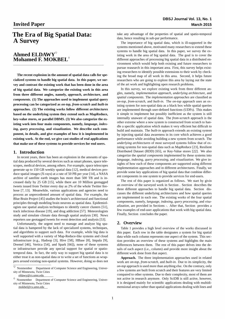
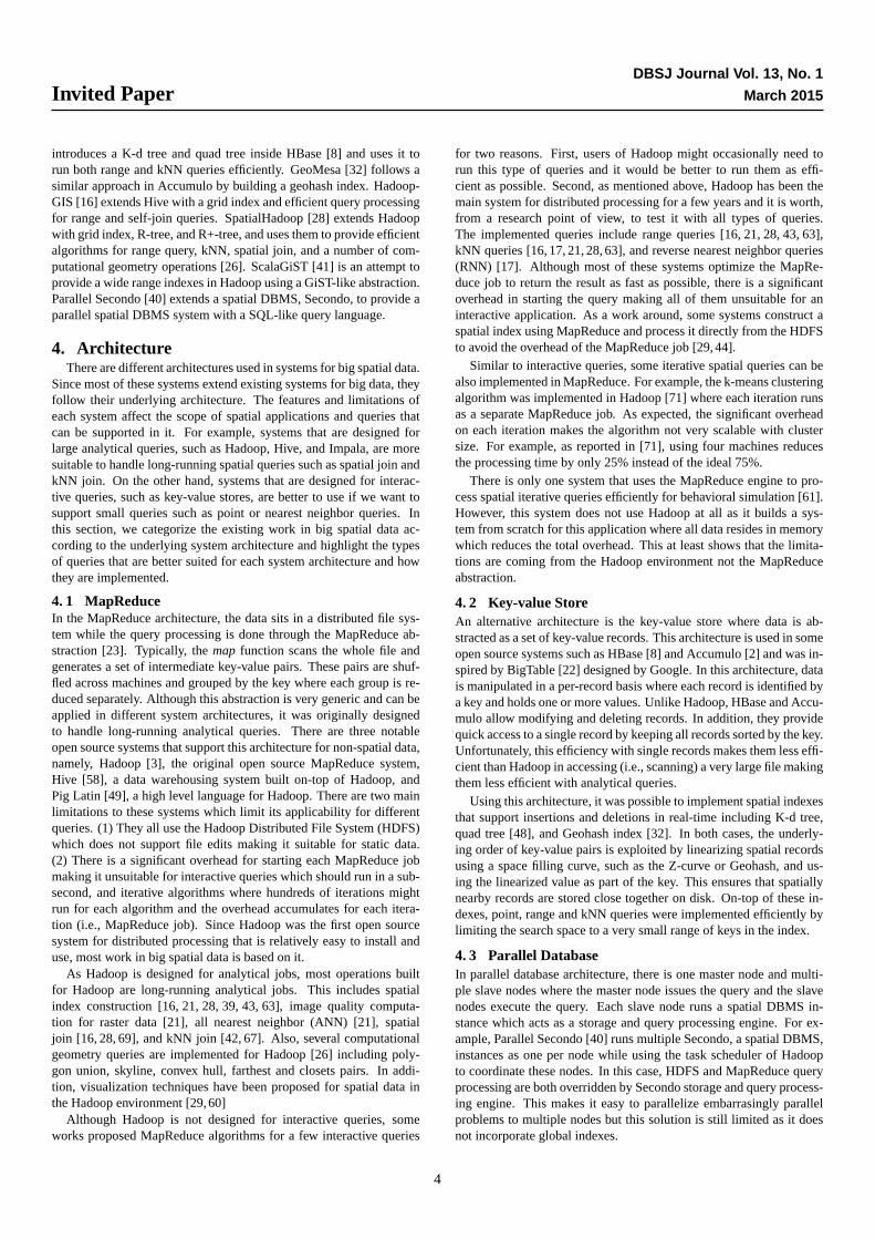
6. 1 Index LayoutThe general layout of spatial indexes created in distributed systemsis a two-layer index of one global index and multiple local indexes.The global index determines how the data is partitioned across ma-chines while local indexes determine how records are stored in eachmachine. This two-layer index lends itself to the distributed environ-ment where there is one master node that stores the global index andmultiple slave nodes that store local indexes. These two levels are or-thogonal which means a system can implement a global-only index, alocal-only index, or both. Besides, there is a flexibility in choosing anytype of index at each of the two levels. Figure 1 gives an example ofan R-tree global index constructed on a 400GB dataset that representsthe road network in the whole world. The blue points in the figurerepresent road segments while the black rectangles represent partitionboundaries of the global index. As shown in figure, this index handlesthe skewness very well by adjusting the size of the partitions such thateach partition contains, roughly, the same amount of data. For exam-ple, dense areas in Europe contain very small rectangles while sparseareas in the oceans contain very large rectangles.

6. 2 Index Bulk LoadingThe most common file system used in open source distributed systemsis the Hadoop Distributed File System. It is already used in Hadoop,Hive, HBase, Spark, Impala and Accumulo. HDFS has a major limi-tation that files can only be written in a sequential manner and, once

5


March 2015

Figure 1: R-tree partitioning of a 400GB road network data

written, cannot be further modified. This rules out most traditional in-dex building techniques as they rely on inserting records one-by-oneor in batches and the index structure evolves as records are inserted.Since HDFS is designed mainly for static data, most techniques focuson bulk loading the index which are described below.

To overcome the limitations of HDFS, most bulk loading techniquesuse a three-phase approach. In the first phase, the space is subdividedinto n partitions by reading a sample of the input file which is thenpartitioned inton partitions of roughly equal sizes. It is expected thatthe sample is a good representative of the data distribution in the orig-inal file. In the second phase, the input file is scanned in parallel, andeach record is assigned to one or more partitions based on its locationand the index type. Records in each partition are then loaded into aseparatelocal index which is stored in the file system. It is expectedthat the size of each partition is small enough to be indexed by a sin-gle machine. In the third phase, thelocal indexes are grouped undera commonglobal index based on their corresponding MBRs; i.e., theMBR of the root node of each local index.

In [16, 28], a uniform grid index is constructed by subdividing thespace using a uniform grid. Notice that in this case, no sample needsto be drawn from the input file as the space is always divided using auniform grid. Then, each record is assigned to all overlapping parti-tions and each partition is written as a heap file; i.e., no local indexingis required. Finally, the global index is created by building a simplein-memory lookup table that stores where each grid cell is stored ondisk.

This technique is also used in [21] to build an R-tree where thespace is subdivided by mapping each point in the random sample toa single number, using a Z-curve, sorting them based on the Z value,and then subdividing the sorted range inton partitions equal to num-ber of machines in the cluster. A similar technique is used in [28] tobuild both R-tree and R+-tree, wheren is first determined by dividingthe file size over the HDFS block capacity to calculate the expectednumber of blocks in the output file. Then, the sample is bulk loadedinto an in-memory R-tree using the STR bulk loading algorithm [38].While partitioning the file, if R-tree is used, each record is assigned toexactly one partition, while in R+-tree, each record is assigned to alloverlapping partitions. This technique is further generalized in [41] tobulk load any tree index described by the GiST abstraction [35].

In [63], a slightly modified technique is used to build a PMR Quadtree. First, a random sample is drawn form the file, linearized usinga Z-curve, and partitioned inton partitions. Then, without spatiallypartitioning the file, each machine loads part of the file and buildsan in-memory PMR Quad tree for that partition. The nodes of eachpartial quad tree are partitioned inton partitions based on their Z-curvevalues. After that, each machine is assigned a partition and merges allnodes in that partition into alocally consistentquad tree. Finally, theselocally consistentquad trees are merged into one final PMR Quad tree.

6. 3 Dynamic Indexes

Some applications require a dynamic index that accommodates inser-tions and deletions of highly dynamic data, such as geotagged tweets,moving objects, and sensor data. In this case, static indexes con-structed using bulk loading cannot work. HBase [8] and Accumulo [2]provide a layer on top of HDFS that allows key-value records to bedynamically inserted and deleted. Modification of records is accom-modated by using a multi-versioning system where each change is ap-pended with a new timestamp. In addition, these systems keep allrecords sorted by the key which allows efficient access to a singlerecord or small ranges of consecutive records. These systems are uti-lized to build dynamic indexes for spatial data as follow.

MD-HBase [48] extends HBase to support both quad tree and K-dtree indexes where the index contains points only. In this approach,each point is inserted as a record in HBase where the key is calculatedby mapping the two-dimensional point location to a single value on theZ-curve. This means that all points are sorted based on the Z-curve.After that, the properties of the Z-curve allows the sorted order to beviewed as either a quad tree or a K-d tree. This structure is utilizedto run both range and kNN queries efficiently. This technique is alsoapplies in [32] to build a geohash index in Accumulo but it extendsthe work in two directions. First, it constructs a spatio-temporal indexby interleaving the time dimension with the geohash of the spatial di-mensions. Second, it supports polygons and polylines by replicatingeach record to all overlapping values on the Z-curve. Although thesesystems provide dynamic indexes, they are designed and optimized forpoint queries which inserts or retrieves a single record. They can stillrun a MapReduce job on the constructed index, but the performance isrelatively poor compared to MapReduce jobs in Hadoop.

6


March 2015

SciDB [56] supports an efficient dynamic K-d tree index as it isdesigned for high dimensional data. Similar to HBase, SciDB usesmulti-versioning to accommodate updates and records are kept sortedusing their keys. However, unlike HBase and Accumulo, the key isallowed to be multidimensional which makes it ready to store spatialpoints. This technique is not directly applicable to lines or polygonsas a line or polygon cannot be assigned a single key.

6. 4 Secondary IndexesSimilar to traditional DBMS, distributed systems can build either aprimary index or a secondary index. In the primary index, recordsare physically reordered on the disk to match the index, while in sec-ondary index, records are kept in their original order while the indexpoints to their offset in the file. In HDFS, secondary indexes performvery poorly due to the huge overhead associated with random file ac-cess [39]. Therefore, most existing indexing techniques focus on pri-mary indexing. There are only two notable works that implement sec-ondary indexes [41, 63]. In both cases, the index is bulk loaded asdescribed earlier but instead of storing the whole record, it only storesthe offset of each record in the file. As clearly shown in [63], the per-formance of the secondary index is very poor compared to a primaryindex and is thus not recommended. However, it could be inevitable tohave a secondary index if users need to build multiple indexes on thesame file.

6. 5 Access MethodsCreating the index on disk is just the first part of the indexing process,the second part, which completes the design, is adding new compo-nents which allow the indexes to be used in query processing. Withoutthese components, the query processing layer will not be able to usethese indexes and will end up scanning the whole file as if there wereno index constructed. Most of the works discussed above do not men-tion clearly the abstraction they provide to the query processing logicand describe their query processing directly. This is primarily becausethey focus on specific queries and they describe how they are imple-mented. However, it is described in [28] that the index constructed inHadoop is made accessible to MapReduce programs through two com-ponents, namely, SpatialFileSplitter and SpatialRecordReader. TheSpatialFileSplitter accesses the global index with a user-defined filterfunction to prune file partitions that do not contribute to answer (e.g.,outside the user-specified query range). The SpatialRecordReader isused to process non-pruned partitions efficiently by using the local in-dex stored in each one.

This separation between the index structure on the file system andthe access methods used in query processing provides the flexibility toreuse indexes. For example, all of Hadoop, Hive, Spark, and Impalacan read their input from raw files in HDFS. This means that one indexappropriately stored in HDFS can be accessed by all these systems ifthe correct access methods are implemented. This also means that wecan, for example, construct the index using a Hadoop MapReduce job,and query that index from Hive using HiveQL.

7. QueryingA main part of any system for big spatial data is the query process-

ing engine. Different systems would probably use different process-ing engines such as MapReduce for Hadoop and Resilient DistributedDataset (RDD) for Spark. While each application requires a differ-ent set of operations, the system cannot ship with all possible spatialqueries. Therefore, the query processing engine should be extensibleto allow users to express custom operations while making use of thespatial indexes. To give some concrete examples, we will describe fivecategories of operations, namely, basic query operations, join opera-

tions, computational geometry operations, data mining operations, andraster operations.

7. 1 Basic Query OperationsThe basic spatial query operations include, point, range, and nearestneighbor queries. We give examples of how these operations are im-plemented in different systems, with, and without indexes.

Point and Range Queries:In a range query, the input is a set ofrecordsR a rectangular query rangeA while the output is the set ofall records inR overlappingA. A point query is a special case wherethe query range has a zero width and height. In [68], a brute forcealgorithm for range queries is implemented in MapReduce by scan-ning the whole file and selecting records that match the query area.In [16,28,63], the constructed index is utilized where the global indexis first used to find partitions that overlap the query range and thenthe local indexes, if constructed, are used to quickly find records inthe final answer. The reference point [25] duplicate avoidance tech-nique is used to eliminate redundant records in the answer if the indexcontains replication. Although this technique is efficient in design, itperforms bad for point queries and small ranges as it suffers from theoverhead of starting a MapReduce job. This overhead is avoided inGeoMesa [32] andMD-HBase [48], as they run on a key-value storewhich is more efficient for this kind of queries. In Hadoop, some ap-plications [18,29,44] achieve an interactive response for range queriesby bypassing the MapReduce engine and running the query against theindex on the file system directly.

nearest neighbor (NN) queries:There are different variations of NNqueries but the most common one is the kNN query. The kNN querytakes a set of pointsP, a query pointQ, and an integerk as input whilethe output is thek closest points inP to Q. In [16, 68], a brute forcetechnique is implemented in MapReduce where the input is scanned,the distance of each pointp ∈ P to Q is calculated, points are sortedbased on distance, and finally top-k points are selected. In [28,48,63],the constructed indexes are used by first searching the partition thatcontains the query point and then expanding the search, as needed, toadjacent partitions until the answer is complete. In [17], a differentapproach is used where a Voronoi diagram is constructed for the inputfile first, and then the properties of this diagram is used to answer kNNqueries. In addition to kNN query, this Voronoi diagram is also used toanswer both reverse NN (RNN) and maximal reverse NN (MaxRNN)queries. In [62], the all nearest neighbor (ANN) query is implementedin MapReduce which finds the nearest neighbor for each point in agiven set of points. It works as two MapReduce jobs where the firstone partitions the data using a Z-curve to group nearby points together,and finds the answer for points which are colocated with their NN inthe same partition. The second MapReduce job finds the NN for allremaining points using the brute-force technique.

7. 2 Join OperationsSpatial Join: In spatial join, the input is two setsR andS and a spatialjoin predicateθ (e.g., touches, overlaps or contains), and the outputis the set of all pairs〈r, s〉 wherer ∈ R, s ∈ S and the join predi-cateθ is true for〈r, s〉. If the input files are not indexed, the partitionbased spatial-merge (PBSM) join algorithm is used where the inputfiles are copartitioned using a uniform grid and the contents of eachgrid cell are joined independently. This technique is implemented inHadoop [69], Impala and Spark [64], without major modifications. Amore efficient algorithm is provided in [16] for the special case ofself-join when the input file is indexed using a uniform grid. In this al-gorithm, the partition step is avoided and the records in each grid cellare directly joined. In [28], a more efficient algorithm is implementedwhich provides a more general join algorithm for two files when one

7


March 2015

c1

c2

c3

c4

c5 c6

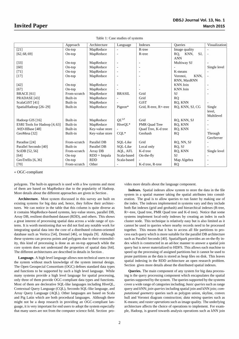
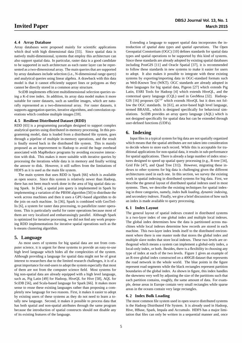
Figure 2: Pruning in skyline

or both files are indexed. If both files are indexed, it finds every pairof overlapping partitions and each pair is processed independently bya map task which applies an in-memory spatial join algorithm, such asthe plane-sweep algorithm. If only one file is indexed, it partitions theother file on-the-fly such that each partition corresponds to one par-tition in the indexed file. This allows a one-to-one mapping betweenthe partitions of the two files making it very efficient to join each pairindependently.kNN Join: Another join operation is the kNN join where the inputis two datasets of pointsR andS , and we want to find for each pointr ∈ R, its k nearest neighbors inS . In [67], a brute force technique isproposed which calculates all pairwise distances between every pair ofpointsr ∈ R ands ∈ S , sorts all of them, and finds the top-k for eachpoint r. A more efficient technique is proposed in the same work butit provides an approximate answer. The later technique first partitionsall points based on a Z-curve, and finds the kNN for each point withinits partition. In [42] an efficient and exact algorithm is provided for thekNN join query which runs in two MapReduce jobs. In the first job,all data is partitioned based on a Voronoi diagram and a partial answeris computed only for points which are colocated with their kNN in thesame partition. In the second phase, the kNN of all remaining pointsis calculated using the brute-force technique.

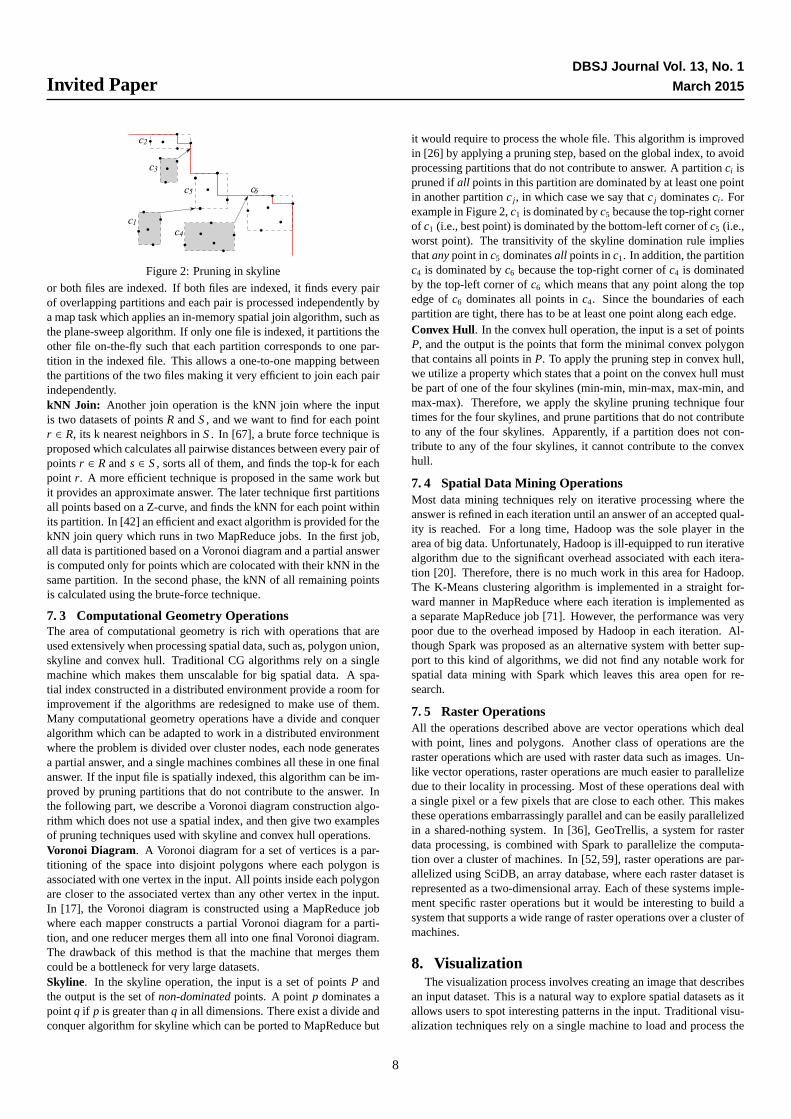
7. 3 Computational Geometry OperationsThe area of computational geometry is rich with operations that areused extensively when processing spatial data, such as, polygon union,skyline and convex hull. Traditional CG algorithms rely on a singlemachine which makes them unscalable for big spatial data. A spa-tial index constructed in a distributed environment provide a room forimprovement if the algorithms are redesigned to make use of them.Many computational geometry operations have a divide and conqueralgorithm which can be adapted to work in a distributed environmentwhere the problem is divided over cluster nodes, each node generatesa partial answer, and a single machines combines all these in one finalanswer. If the input file is spatially indexed, this algorithm can be im-proved by pruning partitions that do not contribute to the answer. Inthe following part, we describe a Voronoi diagram construction algo-rithm which does not use a spatial index, and then give two examplesof pruning techniques used with skyline and convex hull operations.Voronoi Diagram. A Voronoi diagram for a set of vertices is a par-titioning of the space into disjoint polygons where each polygon isassociated with one vertex in the input. All points inside each polygonare closer to the associated vertex than any other vertex in the input.In [17], the Voronoi diagram is constructed using a MapReduce jobwhere each mapper constructs a partial Voronoi diagram for a parti-tion, and one reducer merges them all into one final Voronoi diagram.The drawback of this method is that the machine that merges themcould be a bottleneck for very large datasets.Skyline. In the skyline operation, the input is a set of pointsP andthe output is the set ofnon-dominatedpoints. A pointp dominates apointq if p is greater thanq in all dimensions. There exist a divide andconquer algorithm for skyline which can be ported to MapReduce but

it would require to process the whole file. This algorithm is improvedin [26] by applying a pruning step, based on the global index, to avoidprocessing partitions that do not contribute to answer. A partitionci ispruned ifall points in this partition are dominated by at least one pointin another partitionc j, in which case we say thatc j dominatesci. Forexample in Figure 2,c1 is dominated byc5 because the top-right cornerof c1 (i.e., best point) is dominated by the bottom-left corner ofc5 (i.e.,worst point). The transitivity of the skyline domination rule impliesthatanypoint inc5 dominatesall points inc1. In addition, the partitionc4 is dominated byc6 because the top-right corner ofc4 is dominatedby the top-left corner ofc6 which means that any point along the topedge ofc6 dominates all points inc4. Since the boundaries of eachpartition are tight, there has to be at least one point along each edge.Convex Hull. In the convex hull operation, the input is a set of pointsP, and the output is the points that form the minimal convex polygonthat contains all points inP. To apply the pruning step in convex hull,we utilize a property which states that a point on the convex hull mustbe part of one of the four skylines (min-min, min-max, max-min, andmax-max). Therefore, we apply the skyline pruning technique fourtimes for the four skylines, and prune partitions that do not contributeto any of the four skylines. Apparently, if a partition does not con-tribute to any of the four skylines, it cannot contribute to the convexhull.

7. 4 Spatial Data Mining OperationsMost data mining techniques rely on iterative processing where theanswer is refined in each iteration until an answer of an accepted qual-ity is reached. For a long time, Hadoop was the sole player in thearea of big data. Unfortunately, Hadoop is ill-equipped to run iterativealgorithm due to the significant overhead associated with each itera-tion [20]. Therefore, there is no much work in this area for Hadoop.The K-Means clustering algorithm is implemented in a straight for-ward manner in MapReduce where each iteration is implemented asa separate MapReduce job [71]. However, the performance was verypoor due to the overhead imposed by Hadoop in each iteration. Al-though Spark was proposed as an alternative system with better sup-port to this kind of algorithms, we did not find any notable work forspatial data mining with Spark which leaves this area open for re-search.

7. 5 Raster OperationsAll the operations described above are vector operations which dealwith point, lines and polygons. Another class of operations are theraster operations which are used with raster data such as images. Un-like vector operations, raster operations are much easier to parallelizedue to their locality in processing. Most of these operations deal witha single pixel or a few pixels that are close to each other. This makesthese operations embarrassingly parallel and can be easily parallelizedin a shared-nothing system. In [36], GeoTrellis, a system for rasterdata processing, is combined with Spark to parallelize the computa-tion over a cluster of machines. In [52, 59], raster operations are par-allelized using SciDB, an array database, where each raster dataset isrepresented as a two-dimensional array. Each of these systems imple-ment specific raster operations but it would be interesting to build asystem that supports a wide range of raster operations over a cluster ofmachines.

8. VisualizationThe visualization process involves creating an image that describes

an input dataset. This is a natural way to explore spatial datasets as itallows users to spot interesting patterns in the input. Traditional visu-alization techniques rely on a single machine to load and process the

8


March 2015

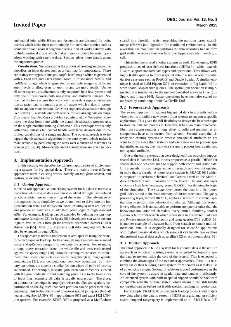
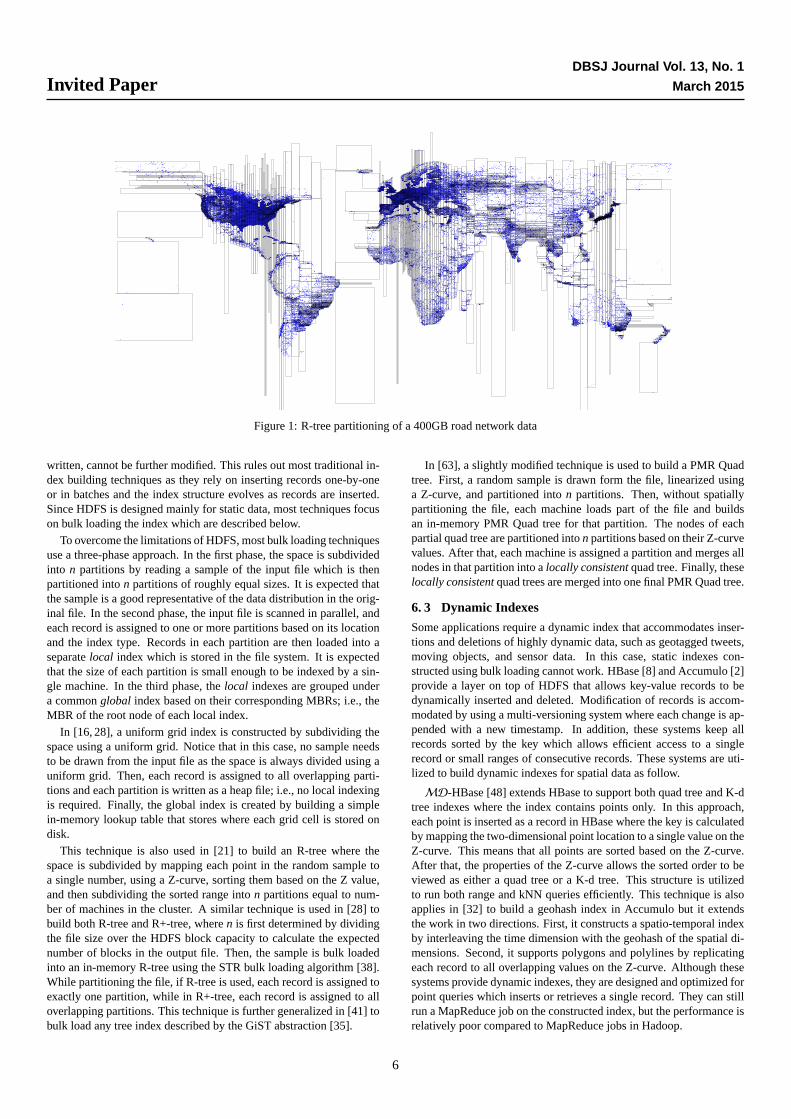
(a) No-cleaning (b) Cleaned data

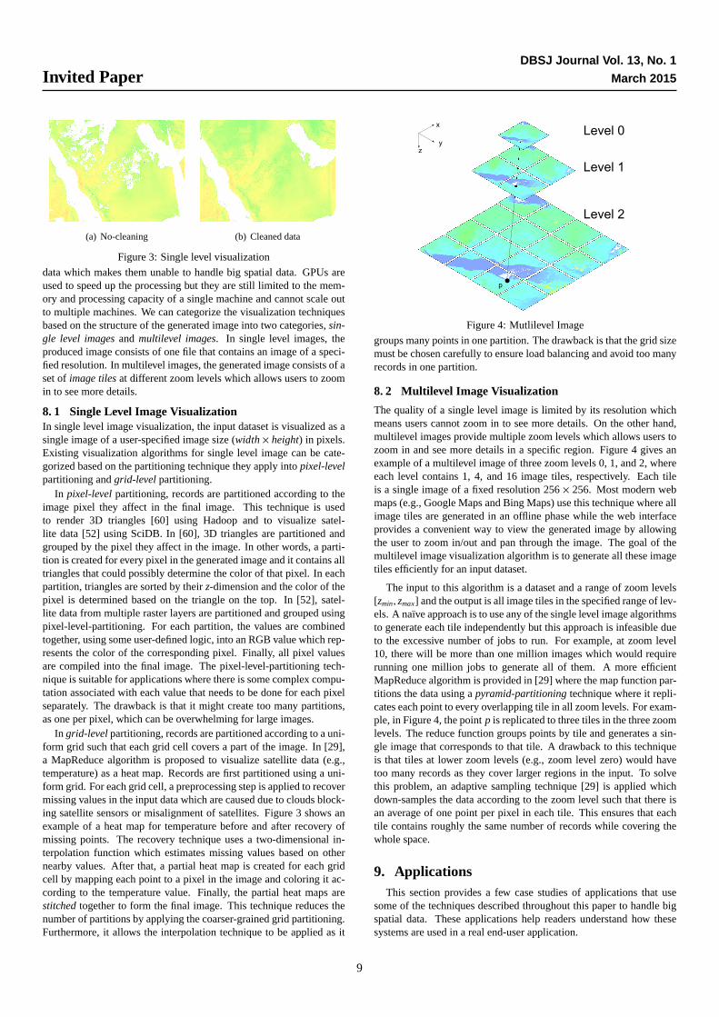
Figure 3: Single level visualization

data which makes them unable to handle big spatial data. GPUs areused to speed up the processing but they are still limited to the mem-ory and processing capacity of a single machine and cannot scale outto multiple machines. We can categorize the visualization techniquesbased on the structure of the generated image into two categories,sin-gle level imagesand multilevel images. In single level images, theproduced image consists of one file that contains an image of a speci-fied resolution. In multilevel images, the generated image consists of aset ofimage tilesat different zoom levels which allows users to zoomin to see more details.

8. 1 Single Level Image VisualizationIn single level image visualization, the input dataset is visualized as asingle image of a user-specified image size (width × height) in pixels.Existing visualization algorithms for single level image can be cate-gorized based on the partitioning technique they apply intopixel-levelpartitioning andgrid-levelpartitioning.

In pixel-levelpartitioning, records are partitioned according to theimage pixel they affect in the final image. This technique is usedto render 3D triangles [60] using Hadoop and to visualize satel-lite data [52] using SciDB. In [60], 3D triangles are partitioned andgrouped by the pixel they affect in the image. In other words, a parti-tion is created for every pixel in the generated image and it contains alltriangles that could possibly determine the color of that pixel. In eachpartition, triangles are sorted by theirz-dimension and the color of thepixel is determined based on the triangle on the top. In [52], satel-lite data from multiple raster layers are partitioned and grouped usingpixel-level-partitioning. For each partition, the values are combinedtogether, using some user-defined logic, into an RGB value which rep-resents the color of the corresponding pixel. Finally, all pixel valuesare compiled into the final image. The pixel-level-partitioning tech-nique is suitable for applications where there is some complex compu-tation associated with each value that needs to be done for each pixelseparately. The drawback is that it might create too many partitions,as one per pixel, which can be overwhelming for large images.

In grid-levelpartitioning, records are partitioned according to a uni-form grid such that each grid cell covers a part of the image. In [29],a MapReduce algorithm is proposed to visualize satellite data (e.g.,temperature) as a heat map. Records are first partitioned using a uni-form grid. For each grid cell, a preprocessing step is applied to recovermissing values in the input data which are caused due to clouds block-ing satellite sensors or misalignment of satellites. Figure 3 shows anexample of a heat map for temperature before and after recovery ofmissing points. The recovery technique uses a two-dimensional in-terpolation function which estimates missing values based on othernearby values. After that, a partial heat map is created for each gridcell by mapping each point to a pixel in the image and coloring it ac-cording to the temperature value. Finally, the partial heat maps arestitchedtogether to form the final image. This technique reduces thenumber of partitions by applying the coarser-grained grid partitioning.Furthermore, it allows the interpolation technique to be applied as it

Level 0

Level 1

Level 2

p

y

x

z

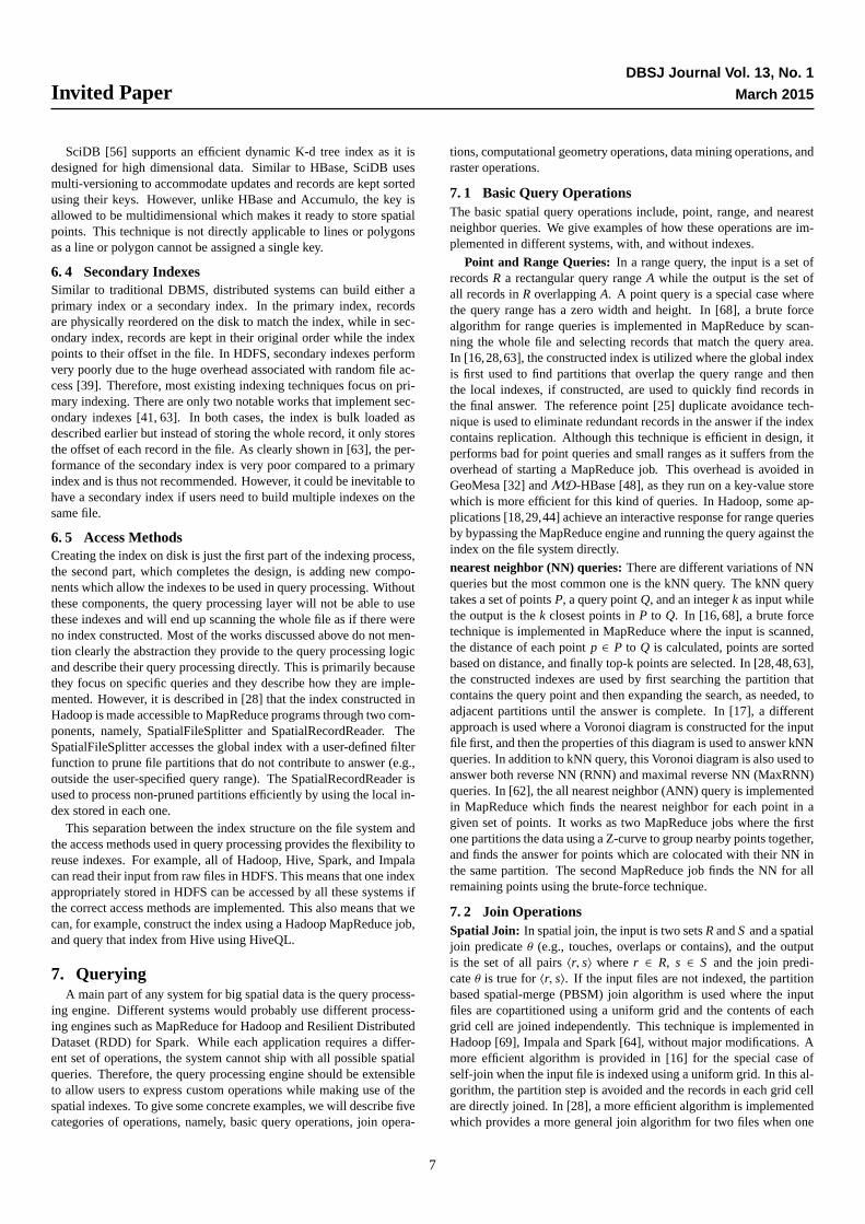
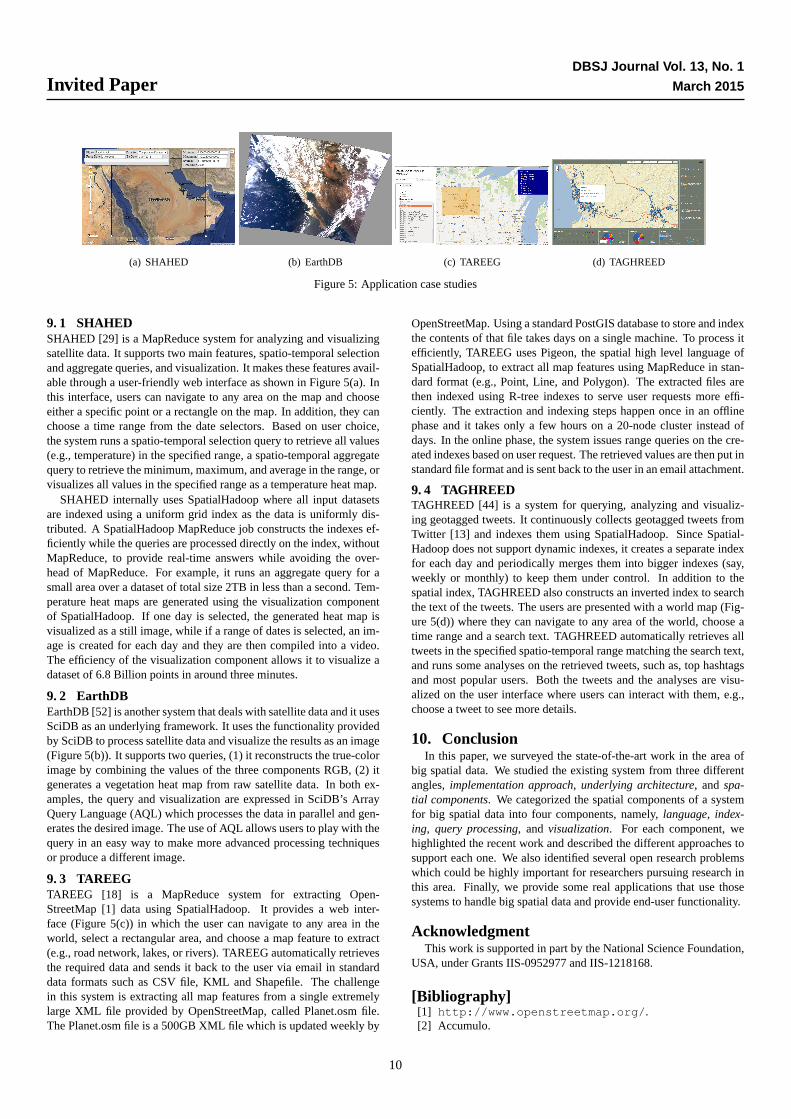
Figure 4: Mutlilevel Image

groups many points in one partition. The drawback is that the grid sizemust be chosen carefully to ensure load balancing and avoid too manyrecords in one partition.

8. 2 Multilevel Image Visualization

The quality of a single level image is limited by its resolution whichmeans users cannot zoom in to see more details. On the other hand,multilevel images provide multiple zoom levels which allows users tozoom in and see more details in a specific region. Figure 4 gives anexample of a multilevel image of three zoom levels 0, 1, and 2, whereeach level contains 1, 4, and 16 image tiles, respectively. Each tileis a single image of a fixed resolution256 × 256. Most modern webmaps (e.g., Google Maps and Bing Maps) use this technique where allimage tiles are generated in an offline phase while the web interfaceprovides a convenient way to view the generated image by allowingthe user to zoom in/out and pan through the image. The goal of themultilevel image visualization algorithm is to generate all these imagetiles efficiently for an input dataset.

The input to this algorithm is a dataset and a range of zoom levels[zmin, zmax] and the output is all image tiles in the specified range of lev-els. A naıve approach is to use any of the single level image algorithmsto generate each tile independently but this approach is infeasible dueto the excessive number of jobs to run. For example, at zoom level10, there will be more than one million images which would requirerunning one million jobs to generate all of them. A more efficientMapReduce algorithm is provided in [29] where the map function par-titions the data using apyramid-partitioningtechnique where it repli-cates each point to every overlapping tile in all zoom levels. For exam-ple, in Figure 4, the pointp is replicated to three tiles in the three zoomlevels. The reduce function groups points by tile and generates a sin-gle image that corresponds to that tile. A drawback to this techniqueis that tiles at lower zoom levels (e.g., zoom level zero) would havetoo many records as they cover larger regions in the input. To solvethis problem, an adaptive sampling technique [29] is applied whichdown-samples the data according to the zoom level such that there isan average of one point per pixel in each tile. This ensures that eachtile contains roughly the same number of records while covering thewhole space.

9. ApplicationsThis section provides a few case studies of applications that use

some of the techniques described throughout this paper to handle bigspatial data. These applications help readers understand how thesesystems are used in a real end-user application.

9


March 2015

(a) SHAHED (b) EarthDB (c) TAREEG (d) TAGHREED

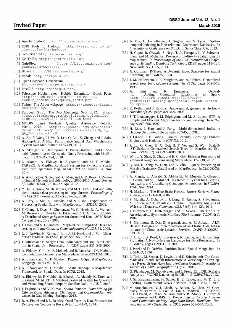
Figure 5: Application case studies

9. 1 SHAHEDSHAHED [29] is a MapReduce system for analyzing and visualizingsatellite data. It supports two main features, spatio-temporal selectionand aggregate queries, and visualization. It makes these features avail-able through a user-friendly web interface as shown in Figure 5(a). Inthis interface, users can navigate to any area on the map and chooseeither a specific point or a rectangle on the map. In addition, they canchoose a time range from the date selectors. Based on user choice,the system runs a spatio-temporal selection query to retrieve all values(e.g., temperature) in the specified range, a spatio-temporal aggregatequery to retrieve the minimum, maximum, and average in the range, orvisualizes all values in the specified range as a temperature heat map.

SHAHED internally uses SpatialHadoop where all input datasetsare indexed using a uniform grid index as the data is uniformly dis-tributed. A SpatialHadoop MapReduce job constructs the indexes ef-ficiently while the queries are processed directly on the index, withoutMapReduce, to provide real-time answers while avoiding the over-head of MapReduce. For example, it runs an aggregate query for asmall area over a dataset of total size 2TB in less than a second. Tem-perature heat maps are generated using the visualization componentof SpatialHadoop. If one day is selected, the generated heat map isvisualized as a still image, while if a range of dates is selected, an im-age is created for each day and they are then compiled into a video.The efficiency of the visualization component allows it to visualize adataset of 6.8 Billion points in around three minutes.

9. 2 EarthDBEarthDB [52] is another system that deals with satellite data and it usesSciDB as an underlying framework. It uses the functionality providedby SciDB to process satellite data and visualize the results as an image(Figure 5(b)). It supports two queries, (1) it reconstructs the true-colorimage by combining the values of the three components RGB, (2) itgenerates a vegetation heat map from raw satellite data. In both ex-amples, the query and visualization are expressed in SciDB’s ArrayQuery Language (AQL) which processes the data in parallel and gen-erates the desired image. The use of AQL allows users to play with thequery in an easy way to make more advanced processing techniquesor produce a different image.

9. 3 TAREEGTAREEG [18] is a MapReduce system for extracting Open-StreetMap [1] data using SpatialHadoop. It provides a web inter-face (Figure 5(c)) in which the user can navigate to any area in theworld, select a rectangular area, and choose a map feature to extract(e.g., road network, lakes, or rivers). TAREEG automatically retrievesthe required data and sends it back to the user via email in standarddata formats such as CSV file, KML and Shapefile. The challengein this system is extracting all map features from a single extremelylarge XML file provided by OpenStreetMap, called Planet.osm file.The Planet.osm file is a 500GB XML file which is updated weekly by

OpenStreetMap. Using a standard PostGIS database to store and indexthe contents of that file takes days on a single machine. To process itefficiently, TAREEG uses Pigeon, the spatial high level language ofSpatialHadoop, to extract all map features using MapReduce in stan-dard format (e.g., Point, Line, and Polygon). The extracted files arethen indexed using R-tree indexes to serve user requests more effi-ciently. The extraction and indexing steps happen once in an offlinephase and it takes only a few hours on a 20-node cluster instead ofdays. In the online phase, the system issues range queries on the cre-ated indexes based on user request. The retrieved values are then put instandard file format and is sent back to the user in an email attachment.

9. 4 TAGHREEDTAGHREED [44] is a system for querying, analyzing and visualiz-ing geotagged tweets. It continuously collects geotagged tweets fromTwitter [13] and indexes them using SpatialHadoop. Since Spatial-Hadoop does not support dynamic indexes, it creates a separate indexfor each day and periodically merges them into bigger indexes (say,weekly or monthly) to keep them under control. In addition to thespatial index, TAGHREED also constructs an inverted index to searchthe text of the tweets. The users are presented with a world map (Fig-ure 5(d)) where they can navigate to any area of the world, choose atime range and a search text. TAGHREED automatically retrieves alltweets in the specified spatio-temporal range matching the search text,and runs some analyses on the retrieved tweets, such as, top hashtagsand most popular users. Both the tweets and the analyses are visu-alized on the user interface where users can interact with them, e.g.,choose a tweet to see more details.

10. ConclusionIn this paper, we surveyed the state-of-the-art work in the area of

big spatial data. We studied the existing system from three differentangles,implementation approach, underlying architecture, andspa-tial components. We categorized the spatial components of a systemfor big spatial data into four components, namely,language, index-ing, query processing, and visualization. For each component, wehighlighted the recent work and described the different approaches tosupport each one. We also identified several open research problemswhich could be highly important for researchers pursuing research inthis area. Finally, we provide some real applications that use thosesystems to handle big spatial data and provide end-user functionality.

AcknowledgmentThis work is supported in part by the National Science Foundation,

USA, under Grants IIS-0952977 and IIS-1218168.

[Bibliography][1] http://www.openstreetmap.org/ .[2] Accumulo.

10


March 2015

[3] Apache. Hadoop.http://hadoop.apache.org/ .

[4] ESRI Tools for Hadoop. http://esri.github.io/gis-tools-for-hadoop/ .

[5] GeoServer.http://geoserver.org/ .[6] GeoTrellis.http://geotrellis.io/ .[7] GnipBlog. https://blog.gnip.com/tag/

geotagged-tweets/ .[8] HBase.http://hbase.apache.org/ .[9] Impala. http://impala.io/ .

[10] Open Geospatial Consortium.http://www.opengeospatial.org/ .

[11] PostGIS.http://postgis.net/ .[12] Telescope Hubbel site: Hubble Essentials: Quick Facts.

http://hubblesite.org/the_telescope/hubble_essentials/quick_facts.php .

[13] Twitter. The About webpage.https://about.twitter.com/company .

[14] European XFEL: The Data Challenge, Sept. 2012.http://www.eiroforum.org/activities/scientific_highlights/201209_XFEL/index.html .

[15] MODIS Land Products Quality Assurance Tutorial:Part:1, 2012. https://lpdaac.usgs.gov/sites/default/files/public/modis/docs/MODIS_LP_QA_Tutorial-1.pdf .

[16] A. Aji, F. Wang, H. Vo, R. Lee, Q. Liu, X. Zhang, and J. Saltz.Hadoop-GIS: A High Performance Spatial Data WarehousingSystem over MapReduce. InVLDB, 2013.

[17] A. Akdogan, U. Demiryurek, F. Banaei-Kashani, and C. Sha-habi. Voronoi-based Geospatial Query Processing with MapRe-duce. InCLOUDCOM, 2010.

[18] L. Alarabi, A. Eldawy, R. Alghamdi, and M. F. Mokbel.TAREEG: A MapReduce-Based System for Extracting SpatialData from OpenStreetMap. InSIGSPATIAL, Dallas, TX, Nov.2014.

[19] A. Auchincloss, S. Gebreab, C. Mair, and A. D. Roux. A Reviewof Spatial Methods in Epidemiology: 2000-2010.Annual Reviewof Public Health, 33:107–22, Apr. 2012.

[20] Y. Bu, B. Howe, M. Balazinska, and M. D. Ernst. HaLoop: effi-cient iterative data processing on large clusters.Proceedings ofthe VLDB Endowment, 3(1-2):285–296, 2010.

[21] A. Cary, Z. Sun, V. Hristidis, and N. Rishe. Experiences onProcessing Spatial Data with MapReduce. InSSDBM, 2009.

[22] F. Chang, J. Dean, S. Ghemawat, W. C. Hsieh, D. A. Wallach,M. Burrows, T. Chandra, A. Fikes, and R. E. Gruber. Bigtable:A Distributed Storage System for Structured Data.ACM Trans.Comput. Syst., 26(2), 2008.

[23] J. Dean and S. Ghemawat. MapReduce: Simplified Data Pro-cessing on Large Clusters.Communications of ACM, 51, 2008.

[24] D. J. DeWitt, N. Kabra, J. Luo, J. M. Patel, and J. Yu. Client-Server Paradise. InVLDB, pages 558–569, 1994.

[25] J. Dittrich and B. Seeger. Data Redundancy and Duplicate Detec-tion in Spatial Join Processing. InICDE, pages 535–546, 2000.

[26] A. Eldawy, Y. Li, M. F. Mokbel, and R. Janardan. CGHadoop:Computational Geometry in MapReduce. InSIGSPATIAL, 2013.

[27] A. Eldawy and M. F. Mokbel. Pigeon: A Spatial MapReduceLanguage. InICDE, 2014.

[28] A. Eldawy and M. F. Mokbel. SpatialHadoop: A MapReduceFramework for Spatial Data. InICDE, 2015.

[29] A. Eldawy, M. F. Mokbel, S. Alharthi, A. Alzaidy, K. Tarek, andS. Ghani. SHAHED: A MapReduce-based System for Queryingand Visualizing Spatio-temporal Satellite Data. InICDE, 2015.

[30] J. Faghmous and V. Kumar.Spatio-Temporal Data Mining forClimate Data: Advances, Challenges, and Opportunities. Ad-vances in Data Mining, Springer, 2013.

[31] R. A. Finkel and J. L. Bentley. Quad Trees: A Data Structure forRetrieval on Composite Keys.Acta Inf., 4:1–9, 1974.

[32] A. Fox, C. Eichelberger, J. Hughes, and S. Lyon. Spatio-temporal Indexing in Non-relational Distributed Databases. InInternational Conference on Big Data, Santa Clara, CA, 2013.

[33] H. Gupta, B. Chawda, S. Negi, T. A. Faruquie, L. V. Subrama-niam, and M. Mohania. Processing multi-way spatial joins onmap-reduce. InProceedings of the 16th International Confer-ence on Extending Database Technology, EDBT, pages 113–124,New York, NY, USA, 2013.

[34] A. Guttman. R-Trees: A Dynamic Index Structure for SpatialSearching. InSIGMOD, 1984.

[35] J. M. Hellerstein, J. F. Naughton, and A. Pfeffer. Generalizedsearch trees for database systems. InVLDB, pages 562–573,1995.

[36] A. Kini and R. Emanuele. Geotrel-lis: Adding Geospatial Capabilities to Spark.http://spark-summit.org/2014/talk/geotrellis-adding-geospatial-capabilities-to-spark .

[37] R. Kothuri and S. Ravada. Oracle spatial, geometries. InEncy-clopedia of GIS., pages 821–826. 2008.

[38] S. T. Leutenegger, J. M. Edgington, and M. A. Lopez. STR: ASimple and Efficient Algorithm for R-Tree Packing. InICDE,pages 497–506, 1997.

[39] H. Liao, J. Han, and J. Fang. Multi-dimensional Index onHadoop Distributed File System.ICNAS, 0, 2010.

[40] J. Lu and R. H. Guting. Parallel Secondo: Boosting DatabaseEngines with Hadoop. InICPADS, 2012.

[41] P. Lu, G. Chen, B. C. Ooi, H. T. Vo, and S. Wu. ScalaG-iST: Scalable Generalized Search Trees for MapReduce Sys-tems.PVLDB, 7(14):1797–1808, 2014.

[42] W. Lu, Y. Shen, S. Chen, and B. C. Ooi. Efficient Processing ofk Nearest Neighbor Joins using MapReduce.PVLDB, 2012.

[43] Q. Ma, B. Yang, W. Qian, and A. Zhou. Query Processing ofMassive Trajectory Data Based on MapReduce. InCLOUDDB,2009.

[44] A. Magdy, L. Alarabi, S. Al-Harthi, M. Musleh, T. Ghanem,S. Ghani, and M. F. Mokbel. Taghreed: A System for Querying,Analyzing, and Visualizing Geotagged Microblogs. InSIGSPA-TIAL, Nov. 2014.

[45] H. Markram. The Blue Brain Project.Nature Reviews Neuro-science, 7(2):153–160, 2006.

[46] S. Melnik, A. Gubarev, J. J. Long, G. Romer, S. Shivakumar,M. Tolton, and T. Vassilakis. Dremel: Interactive Analysis ofWeb-scale Datasets.Commun. ACM, 54(6):114–123, 2011.

[47] J. Nievergelt, H. Hinterberger, and K. Sevcik. The Grid File:An Adaptable, Symmetric Multikey File Structure.TODS, 9(1),1984.

[48] S. Nishimura, S. Das, D. Agrawal, and A. El Abbadi.MD-HBase: Design and Implementation of an Elastic Data Infras-tructure for Cloud-scale Location Services.DAPD, 31(2):289–319, 2013.

[49] C. Olston, B. Reed, U. Srivastava, R. Kumar, and A. Tomkins.Pig Latin: A Not-so-foreign Language for Data Processing. InSIGMOD, pages 1099–1110, 2008.

[50] J. Patel and D. DeWitt. Partition Based Spatial-Merge Join. InSIGMOD, 1996.

[51] L. Pickle, M. Szczur, D. Lewis, , and D. Stinchcomb. The Cross-roads of GIS and Health Information: A Workshop on Develop-ing a Research Agenda to Improve Cancer Control.InternationalJournal of Health Geographics, 5(1):51, 2006.

[52] G. Planthaber, M. Stonebraker, and J. Frew. EarthDB: ScalableAnalysis of MODIS Data using SciDB. InBIGSPATIAL, 2012.

[53] J. Sankaranarayanan, H. Samet, B. E. Teitler, and M. D. L. J.Sperling. TwitterStand: News in Tweets. InSIGSPATIAL, 2009.

[54] M. Stonebraker, D. J. Abadi, A. Batkin, X. Chen, M. Cher-niack, M. Ferreira, E. Lau, A. Lin, S. Madden, E. J. O’Neil,P. E. O’Neil, A. Rasin, N. Tran, and S. B. Zdonik. C-Store: AColumn-oriented DBMS. InProceedings of the 31st Interna-tional Conference on Very Large Data Bases, Trondheim, Nor-way, August 30 - September 2, 2005, pages 553–564, 2005.

11


March 2015

[55] M. Stonebraker, P. Brown, A. Poliakov, and S. Raman. The Ar-chitecture of SciDB. InSSDBM, 2011.

[56] M. Stonebraker, P. Brown, D. Zhang, and J. Becla. SciDB: ADatabase Management System for Applications with ComplexAnalytics.Computing in Science and Engineering, 15(3):54–62,2013.

[57] Y. Thomas, D. Richardson, and I. Cheung. Geography and DrugAddiction. Springer Verlag, 2009.

[58] A. Thusoo, J. S. Sen, N. Jain, Z. Shao, P. Chakka, S. Anthony,H. Liu, P. Wyckoff, and R. Murthy. Hive: A Warehousing Solu-tion over a Map-Reduce Framework.PVLDB, pages 1626–1629,2009.

[59] J. VanderPlas, E. Soroush, K. S. Krughoff, and M. Balazinska.Squeezing a Big Orange into Little Boxes: The AscotDB Systemfor Parallel Processing of Data on a Sphere.IEEE Data Eng.Bull., 36(4):11–20, 2013.

[60] H. T. Vo, J. Bronson, B. Summa, J. L. D. Comba, J. Freire,B. Howe, V. Pascucci, and C. T. Silva. Parallel Visualizationon Large Clusters using MapReduce. InIEEE Symposium onLarge Data Analysis and Visualization, LDAV, 2011.

[61] G. Wang, M. A. V. Salles, B. Sowell, X. Wang, T. Cao, A. J.Demers, J. Gehrke, and W. M. White. Behavioral Simulations inMapReduce.PVLDB, 3(1):952–963, 2010.

[62] K. Wang, J. Han, B. Tu, J. D. amd Wei Zhou, and X. Song. Ac-celerating Spatial Data Processing with MapReduce. InICPADS,2010.

[63] R. T. Whitman, M. B. Park, S. A. Ambrose, and E. G. Hoel. Spa-tial Indexing and Analytics on Hadoop. InSIGSPATIAL, 2014.

[64] S. You, J. Zhang, and L. Gruenwald. Large-Scale Spatial JoinQuery Processing in Cloud. Technical report, The City Collegeof New York, New York, NY.

[65] M. Zaharia, M. Chowdhury, T. Das, A. Dave, J. Ma, M. Mc-Cauly, M. J. Franklin, S. Shenker, and I. Stoica. Resilient Dis-tributed Datasets: A Fault-Tolerant Abstraction for In-MemoryCluster Computing. pages 15–28, 2012.

[66] M. Zaharia, M. Chowdhury, M. J. Franklin, S. Shenker, andI. Stoica. Spark: Cluster Computing with Working Sets. 2010.

[67] C. Zhang, F. Li, and J. Jestes. Efficient Parallel kNN Joins forLarge Data in MapReduce. InEDBT, 2012.

[68] S. Zhang, J. Han, Z. Liu, K. Wang, and S. Feng. Spatial QueriesEvaluation with MapReduce. InGCC, 2009.

[69] S. Zhang, J. Han, Z. Liu, K. Wang, and Z. Xu. SJMR: Paral-lelizing spatial join with MapReduce on clusters. InCLUSTER,2009.

[70] X. Zhang, J. Ai, Z. Wang, J. Lu, and X. Meng. An efficientmulti-dimensional index for cloud data management. InCIKM,pages 17–24, Hong Kong, China, 2009.

[71] W. Zhao, H. Ma, and Q. He. ParallelK-Means Clustering Basedon MapReduce. InCloudCom 2009, pages 674–679, 2009.

Ahmed ELDAWYis a fifth year PhD candidate at the department of Computer Scienceand Engineering, University of Minnesota. He obtained his B.Sc. andMS in Computer Science from Alexandria University in 2005 and2010, respectively. His research interest lies in the broad area of datamanagement systems. Ahmed released his ongoing PhD work, Spa-tialHadoop, as an open source project which has been used by sev-eral companies, organizations and research institutes around the world.During his PhD, he visited IBM T.J. Watson research center, MicrosoftResearch in Redmond, Qatar Computing Research Institute, and GISTechnology Innovation Center in Saudi Arabia. He has been awardedthe University of Minnesota Doctoral Dissertation Fellowship in 2014.

Mohamed F. MOKBEL(Ph.D., Purdue University, USA, MS, B.Sc., Alexandria University,Egypt) is an associate professor at University of Minnesota. He isalso the founding Technical Director of the KACST GIS Technology

Innovation Center, Umm Al-Qura University, Saudi Arabia. His cur-rent research interests focus on database systems, GIS, and big spatialdata. His research work has been recognized by four best paper awardsand by the NSF CAREER award 2010. Mohamed is/was general co-chair of SSTD 2011, program co-chair of ACM SIGSPATIAL GIS2008-2010, and IEEE MDM 2011, 2014. He is in the editorial boardof ACM Transactions on Spatial Algorithms and Systems and ACMTransactions on Database Systems. Mohamed has held various visit-ing positions at Microsoft Research, USA and Hong Kong Polytech-nic University. Mohamed is a founding member of ACM SIGSPA-TIAL and is currently serving as an elected chair of ACM SIGSPA-TIAL for the term 2014-2017. For more information, please visit:www.cs.umn.edu/˜mokbel

12

Documents

The Era of Big Spatial Data: A Survey - UCReldawy/publications/DBSJ_survey.pdf · The Era of Big Spatial Data: A Survey ... of the art work and highlighting open research problems