The Estimates of Environmental National Accounts for ... ·

Gains from Trade Are Not Enough

1

The Estimates of Environmental National Accounts for Venezuela and Mexico over the 20th century: accounting

for depleted oil* Mar Rubio

"Juan de la Cierva" Research Fellow Department of Economics and Business

Universitat Pompeu Fabra Barcelona 08005 Spain

ABSTRACT In principle, a country can not endure negative genuine savings for long periods of time without experiencing declining consumption. Nevertheless, theoreticians envisage two alternatives to explain how an exporter of non-renewable natural resources could experience permanent negative genuine savings and still ensure sustainability. The first one alleges that the capital gains arising from the expected improvement in the terms of trade would suffice to compensate for the negative savings of the resource exporter. The second alternative points at technological change as a way to avoid economic collapse. This paper uses the data of Venezuela and Mexico to empirically test the first of these two hypotheses. The results presented here prove that the terms of trade do not suffice to compensate the depletion of oil reserves in these two open economies.

Keywords: exhaustible resources, environmental accounts, net national product, genuine savings, foreign trade. JEL: Q01, N5, P24, F18

* This paper is a modified version of an earlier paper entitled ‘The Capital Gains from Trade are not Enough: Evidence From the Environmental Accounts of Venezuela and Mexico’, published first as a a working paper at UPF.Comments are welcomed to [email protected]


2

The Estimates of Environmental National Accounts for Venezuela and Mexico over the 20th century: accounting for depleted oil The traditional measure of a nation’s rate of accumulation of wealth is gross saving.

This is calculated as a residual: GNP minus public and private consumption. Gross

saving represents the total amount of produced output that is set aside for the future.

Gross savings rates can say little about the sustainability of development, however,

because productive assets depreciate through time: if this depreciation is greater than

gross saving, then aggregate wealth is in decline. Net saving, total gross saving less

the value of depreciation of produced assets, is one step closer to a sustainability

indicator, but focuses narrowly on produced assets. Environmental economist

assimilate natural resources to man made capital, since a country’s consumption may

be mainly supported by draining natural resources, i.e. from the depreciation of

natural capital. Traditionally computed net savings ignore the depreciation of natural

capital. Once natural capital depreciation is also subtracted we arrive to the concept

of ‘genuine savings’.

Hartwick [20] and Solow [55], building on the concepts of Hicks [23] established that

in order to achieve constant real consumption through time (the lower bound of

sustainability) it is necessary to keep the underlying capital stock constant. It

becomes a requirement that the value of the net change in the total capital stock (that

is the genuine savings) must be equal or greater than zero. In principle, a country can

not therefore endure negative genuine savings for long periods of time without

experiencing declining consumption, or the total collapse of its economy.

Nevertheless, theoreticians have envisaged some possibilities that would allow an

exporter of non-renewable natural resources to experience persistent negative

genuine savings and still ensure sustainability. The first one alleges that the capital

gains arising from the expected improvement in the terms of trade would allow the

resource exporter to compensate for the negative savings. The second alternative

points at technological change as a way to avoid economic collapse. The gains from

trade have now been included in environmental accounting models. Some of the more

representative are those of Asheim [1, 2], Hartwick [22], Newmayer [42], Sefton and

Weale [54] and Weale [64], while the technical change avenue remains largely

unexplored exception made of the contributions of Weitzman [66].

The exercises in this paper use the historical data of Venezuela and Mexico to test ex

post the validity of the predictions of the models that include capital gains from trade

in modifying the genuine savings indicator. Mexico and Venezuela have been oil


3

producers since the dawn of the oil era. Mexico started commercial production in

1901 and was the world’s greatest oil exporter and second producer by 1921.

Venezuela replaced Mexico in this position during the inter-war years. While Mexico

nationalized its oil industry by 1938 and followed an inward-looking strategy of

depleting the oil just to the extent necessary to fulfil domestic requirements,

Venezuela adopted a pure export-oriented strategy, leaving her oil in foreign hands

until 1976. After almost forty years of looking at each other with a mixture of criticism

and wonder, defending their own exploitation strategy as the best possible, Mexico

and Venezuela ended the twentieth century as state-owned medium-sized oil

exporters. The real benefit of ex post analysis is in making the most of the opportunity

to improve the analytical model used as much as in understanding the path that

history took.

The order of exposition in the paper is as follows:

1. The first exercise introduces the concept and computes the value of genuine

savings indicator for the Venezuelan and Mexican economies. By emphasising

the level of genuine savings, we are in effect asking the question: how much of

the net (environmentally adjusted) income was actually consumed? Or in other

words, were the countries living beyond their means? In this first exercise

Venezuela appears to have been living beyond its means for a very long period of

time, yet the expected decline in well-being cannot be observed. Hence, the

prediction of unsustainability implied by negative genuine savings comes into

question.

2. The second exercise examines the role of the terms of trade in modifying the

standard sustainability indicator in two alternative ways:

a) Using the methodology of Sefton and Weale [54] (imputed income method) that

takes into account the expected capital gains from trade for the adjustment of net

income. This second indicator reverses the view of the previous exercise, showing

that Venezuela and Mexico were never consuming beyond their means if the

expected gains from the terms of trade are taken into account.

b) Using one of the methodologies proposed in the national income literature for

assessing the effect of the actual changes in the terms of trade on national

income. The additions to welfare income due to the historical changes in the terms

of trade differ substantially from the expected terms of trade effects derived from

Sefton and Weale model resulting in the return of the paradox of negative genuine

savings without observable declines in well-being.

The exercises of this paper are restricted by the availability of traditional macro-

economic data. In particular, the short series on national income (NNP) shorten the


4

period of analysis to 1936-1985 for Venezuela and to 1950-1989 for Mexico. This

does not affect the main thrust of the argument.

The results of this paper are on line with the findings of Vincent et al. [63], who

estimated that Indonesia would have to invest more in order to sustain its

consumption levels when using an open economy model than using a closed

economy model. These results question the view that the exporter of natural

resources ‘does not have to do any investing in order to maintain its level of income

constant, so the whole of the revenue is available for consumption’ given the

expected gains in the terms of trade (Weale [64], pp.99-100). In the absence of

technical change, consuming the whole of the revenue may be a good theoretical

option but a bad economic decision.

The Standard Sustainability Indicator: Genuine Savings

The genuine savings indicator can be expressed in the form

YK

YK

YSZ NNMM δδ

−−= [1]

where S is gross savings, δMKM and δNKN are man-made capital and natural capital

depreciation respectively and Y is total output in the economy. According to its

authors, Pearce et al. [45], [46], Z ‘is an intuitive zero-order rule for determining

whether a country is on or off a sustainable development path at any one point in

time. The value of Z must be either zero or positive to ensure sustainability.’

By emphasising the level of genuine savings, we are in effect asking the question:

how much of the adjusted income was actually consumed? Gross savings are GNP

minus consumption. Net savings are gross savings minus depreciation of physical

capital, which can also be expressed as (GNP - δMKM )-C = NNP -C . Subtracting

natural capital depreciation from these net savings we arrive to genuine savings,

NNP-δNKN –C = NNPadj-C. Thus the Z indicator can actually be re-expressed in the

following terms:

YCNNP

Z adj −= [2]

where NNPadj is the environmentally adjusted net income (that is, NNP-δNKN) and C is

the sum of public and private consumption. Observe that, in the way it was originally

formulated, the genuine savings indicator implies the use of the net price method of

Repetto et al. [51] for adjusting the traditional NNP. This method establishes that

natural capital depreciation, δNKN, matches the total resource rent (Nt) for the year,

where the usual measure for the resource rent has been the surplus revenue accruing


5

to the owners of the resource after accounting for the contribution of capital and

labour inputs.

Figures 1 and 2 compare the sizes of the man-made capital depreciation (δMKM) as

recorded in the traditional accounts, with the measure of natural capital depreciation

(δNKN), that is Nt, estimated by Rubio [52] for the depletion of oil resources in Mexico

and Venezuela.

Natural resource depreciation –approximated by the depreciation of oil resources- is

larger than physical capital depreciation throughout the period studied in the case of

Venezuela. For Mexico the scale of the natural depreciation cannot be dismissed from

the 1970s onwards. Prior to that date the level of natural capital depreciation for

Mexico was of the order of 1.5 percent of traditional GDP. At least two caveats are

required in relation to this comparison. First, it is worth bearing in mind that the natural

capital depreciation estimates calculated here are only considering a single natural

resource, i.e. oil. It is the resource that generated the greatest rents and therefore the

greatest depreciation during the century, but the depreciation of other natural

resources should ideally be also accounted for (consider, for instance, natural gas).

Therefore, the figures shown here underestimate natural depreciation. In the second

place, the comparison should be regarded with caution since the historical estimates

of consumption of fixed capital are feeble, especially in the case of Mexico. All in all,

however the message from Figures 1 and 2 is clear: natural depreciation is by no

means negligible.


6

Figure 1: Man-made capital VS natural capital depreciation. Venezuela 1920s-1980s (mill. Bolivars current prices)

mill

cur

r bo

livar

s (lo

g)

year

Venezuela,fixed K consumption Oil depreciation (Net Price)

1920 1930 1940 1950 1960 1970 1980

1000

10000

100000

500000

Notes and sources: Fixed capital consumption (δMKM) data sources in Appendix D and natural capital depreciation δNKN from Rubio [52] as listed in Table A.1 in Appendix 1

Figure 2: Man-made capital VS natural capital depreciation.

Mexico1920s-1980s (mill. Pesos current prices (log))

mll

curr

pe

sos

(lo

g)

year

Mexico, fixed K consumption Oil depreciation (Net Price)

1920 1930 1940 1950 1960 1970 1980

3000

100000100000

1.0e+06

5.0e+06

Notes and sources: Fixed capital consumption (δMKM) data sources in Appendix D and natural capital depreciation δNKN from Rubio [52] and listed in Table A.2 in Appendix 1


7

These estimates of natural depreciation are used for the computation of the Z indicator

described in equation [1]. Figures 3 and 4 offer the graphical representation of the

gross, net and genuine savings as percentage of GDP for Mexico and Venezuela.

Figure 3: Genuine savings. Venezuela 1936-1985 (percentage over GDP)

- 2 0 %

- 1 0 %

0 %

1 0 %

2 0 %

3 0 %

4 0 %

5 0 %

1936

1938

1940

1942

1944

1946

1948

1950

1952

1954

1956

1958

1960

1962

1964

1966

1968

1970

1972

1974

1976

1978

1980

1982

1984

% o

f tra

dito

nal G

DP

G r o s s S a v i n g s N e t S a v i n g s G e n u i n e s a v i n g s Source: Table 3

Figure 4: Genuine savings. Mexico 1950-1985 (percentage over GDP)

- 2 0 %

- 1 0 %

0 %

1 0 %

2 0 %

3 0 %

4 0 %

1950

1952

1954

1956

1958

1960

1962

1964

1966

1968

1970

1972

1974

1976

1978

1980

1982

1984

% o

f tra

ditio

nal G

DP

G r o s s S a v in g s N e t s a v in g s G e n u in e s a v in g s

Source: Table 4.


8

This first exercise shows Venezuela’s Z indicator taking negative values by the 1930s

and from 1944 it permanently failed to satisfy the rule in equation [1]. This is a striking

result for an economy historically portrayed as an exceptionally high saver. In 1961

the IBRD reported ‘Venezuela has devoted 30 percent of its GNP to gross

investment, a proportion equalled or exceeded in only a few European countries

notably west Germany and Norway’ [26]. The Mexican indicator only turned negative

only for a couple of years in the early 1980s. These results are on the line of those

reported by Pearce and Atkinson [46](p.173) for Mexico for the year 1985 (0 genuine

savings). The results presented here also coincide with the World Bank [67] (p.12) for

the period 1970-1993, which reports that ‘strong savers like Brazil and Chile are offset

by the genuine dissaving of Venezuela and Ecuador and the near-zero genuine

savings of Mexico’. In theory, these results indicate that Venezuela has been living

beyond its means to a greater extent and for a longer period than Mexico.

According to the World Bank [67] (p.8) ‘persistently negative rates of genuine savings

must lead, eventually, to declining well-being’. The puzzling question regarding this

prediction is: for how long can a country endure negative genuine savings before the

eventual decline of well-being becomes apparent? If Mexican results were the

measure, it could be argued that a couple of years with negative genuine savings are

sufficient to observe a decline in well-being by the mid 1980s. In contrast, in

Venezuela negative rates of genuine savings occurred continuously for over 40 years

and yet, declining well-being was only perceived from the 1980s, and according to

some authors, only from the 1990s onwards (see Coronil [12] and Goodman [15]). Not in vain Venezuela has the best overall performance in Latin America throughout

the twentieth century in terms of traditional GDP growth according to Hofman [24]

(p.87). By any standards the negative rents of Venezuela were persistent enough,

yet the expected decline in well-being was greatly delayed. Hence, the predicted

unsustainability of negative genuine savings comes into question.

As mentioned above, several authors have theorised about the role of capital gains

arising from (1) improved terms of trade and (2) technological change in modifying the

Z>0 rule. The next section tests empirically the first of these theoretical objections to

the genuine savings indicator.

The Effects of the Terms of Trade

The national income literature has long noted the problem that traditional indicators in

‘may not be a good indicator of national welfare in an open economy experiencing

substantial change in its terms of trade.’ Hamada et al. [19] (p.752). This occurs

because traditional measures of output and income fail to account for the impact of


9

changing terms of trade on the consumption possibilities of the economy. Gutman [17]

summarised the many attempts to adjust for the terms of trade impact on the

measurement of national income, although it does not includes the later attempt by

Hamada et al. [19]. The general result from those attempts is in words of Irwin [27]

(p.100) ‘when the terms of trade deteriorated, measures of economic growth tended

to overstate gains in real income; when they improved, those measures understated

such gains.’

This observation has not escaped the analysis of environmental accountants. Sefton

and Weale [54] argued that the net price method is inappropriate for adjusting the net

income for the depletion of oil reserves in open economies precisely because it

ignores the effects on welfare income of the expected improvement of the terms of

trade of an oil exporter (the model explicitly mentioned by Sefton and Weale is not the

net price of Repetto, but Dasgupta et al. [13] and Hartwick [21], which are the

foundations of Repetto’s model). Accordingly, the sustainability rule Z presented in the

section above would differ for open and closed economies. Sefton and Weale derived

the necessary adjustment for an open economy that exports natural resources. Their

suggestion is that the adjusted income would be incomplete without an imputed

income for the stock of the resource targeted for export. This imputed income should

be included in the measures of adjusted income in order to take into account the

effects from the expected gains in the terms of trade. In fact their model suggest two

adjustments: an imputed income for the stock of resource targeted for export and a

rate of interest effect. Yet, the second adjustment is considered ‘harder to estimate

and it seems reasonable to assume is negligible as real interest rates can be

expected to remain almost constant in the long run’ (Sefton and Weale [54] p.46). Appendix 2 offers a brief discussion of Sefton and Weale method. The

environmentally adjusted income corresponding to Sefton and Weale methodology

responds to the following formulation:

Vti

iNNNPNNP tadj ++−=

1

where NNP is the traditionally computed net income, Nt is still the resource rent (the

net price in other words) and the last term corresponds to the expected gains from the

improved terms of trade. In this second exercise, the Z indicator is re-estimated using

equation [2], but rather than adjusting the traditional income by the net price method,

the net income is adjusted by the imputed income method just defined.


10

Figure 5:Genuine Savings Taking into Account the Expected Gains from Trade. Venezuela 1936-1985 (percentage over traditional GDP)

0 .0 %

5 .0 %

1 0 .0 %

1 5 .0 %

2 0 .0 %

2 5 .0 %

3 0 .0 %

3 5 .0 %

4 0 .0 %

4 5 .0 %

1936

1938

1940

1942

1944

1946

1948

1950

1952

1954

1956

1958

1960

1962

1964

1966

1968

1970

1972

1974

1976

1978

1980

1982

1984

% o

f tra

ditio

nal G

DP

G ro ss S a v in g s N e t S a v in g s G e n u in e S a v in g s (S & W )

Sources: Gross and net savings as in Table 3. Genuine savings correspond to the NNP minus the imputed income adjustment in Table A.3 in Appendix 1 (a discount rate of 6% is used here).

Figure 6:Genuine Savings Taking into Account the Expected Gains from Trade. Mexico 1950-1985 (percentage over traditional GDP)

0 %

5 %

1 0 %

1 5 %

2 0 %

2 5 %

3 0 %

3 5 %

4 0 %

1950

1951

1952

1953

1954

1955

1956

1957

1958

1959

1960

1961

1962

1963

1964

1965

1966

1967

1968

1969

1970

1971

1972

1973

1974

1975

1976

1977

1978

1979

1980

1981

1982

1983

1984

1985

% o

f tra

ditio

nal G

DP

G ro ss S a vin g s N e t S a vin g s G e n u in e S a vin g s (S & W )

Sources: Gross and net savings as in Table 4. Genuine savings correspond to the NNP minus the imputed income adjustment in Table A.4 in Appendix 1 (a discount rate of 6% is used here).


11

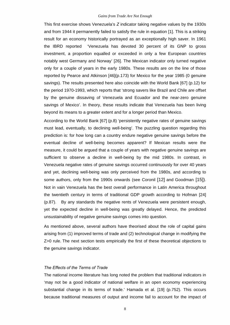
Figures 5 and 6 illustrate the effects of the expected gains from trade in modifying the

Z indicator. When net income is adjusted using the imputed income method, it

appears that Venezuela and Mexico consumed within their means throughout the

period analysed. According to the results the levels of consumption were not

necessarily unsustainable given the expected continuous improvement on the terms

of trade of a resource exporter. However, some important caveats should be taken

into account.

The expected gains from trade in Sefton and Weale method arise from the application

of Hotelling’s rule. That is the expectation that the resource rent is going to grow at

the rate of interest in the economy until the resource is exhausted. But the analysis of

the behaviour of the rents calculated for Mexico and Venezuela in the section above

revealed that there is no historical evidence supporting Hotelling’s principle (rents

have not grown at the rate of interest). Consequently, the possibility of escaping from

negative savings in open economies through the improvement of the terms of trade is

considerably reduced and needs further investigation.

The obvious way to establish the role of the terms of trade is to observe their historical

evolution. Figures 7 and 8 reveal the terms of trade for Venezuela and Mexico for the

relevant periods. Contrary to what would be expected from the application of

Hotelling’s rule, the terms of trade do not improve continuously in either of the two

countries. Venezuelan terms of trade improved markedly from 1942 to 1957 and

during the 1970s, but from the end of the 1958 until 1972 remained constant and from

the early 1980s declined notably. In the case of Mexico, before it re-started its oil

exports, the terms of trade exhibit a modest upward trend; when oil regained a

significant position in Mexican exports from 1974, the terms of trade improved briefly

but started to decline from the 1980s and finally arrived at a constant level. The

historical terms of trade do not satisfy the theoretical predications of the imputed

income method.


12

Figure 7: Venezuelan Terms of Trade, 1928-1989 (1968=100)

1

10

100

1000

1928

1930

1932

1934

1936

1938

1940

1942

1944

1946

1948

1950

1952

1954

1956

1958

1960

1962

1964

1966

1968

1970

1972

1974

1976

1978

1980

1982

1984

1986

1988

% (l

ogs)

T e rm s of trade( B lv)1968=100

Sources: Terms of trade calculated as the ratio between exports and imports price indexes. Export price index was elaborated using the exports and prices series of oil from Appendixes A and B. It is worth recalling that oil exports represent the vast majority of Venezuelan exports for the dates shown. Imports price index from Baptista [9].

Figure 8: Mexican Terms of Trade, 1960-1989 (1995=100)

1 0 .0 0

1 0 0 .0 0

1 0 0 0 .0 0

1960

1961

1962

1963

1964

1965

1966

1967

1968

1969

1970

1971

1972

1973

1974

1975

1976

1977

1978

1979

1980

1981

1982

1983

1984

1985

1986

1987

1988

1989

%

T e r m s o f T ra d e , 1 9 9 5 = 1 0 0

Source : Easterly et al. [14]


13

It is possible to argue that even if the rents had increased at the rates assumed by

Hotelling’s rule, the gains from the terms from trade may have not continuously

increased. Some of the gains apparently associated with the improved terms from

trade may be lost since oil is a basic input for producing the goods that the oil-

exporter-country needs to import. This is actually a common assumption in models

that take natural resources into account (for instance Sefton and Weale [54]). Higher

oil prices will influence the price of imports and the gains from the terms of trade will

be reduced. The theoretical models do not consider this feedback effect.

These results do not overrule the fact that the terms of trade have an effect in

modifying the Z indicator. Although Mexico and Venezuela did not experience the

continuous improvement in the terms of trade implicitly assumed by the imputed

income method, both countries were at different points in time open economies

experiencing substantial changes in their terms of trade. As a consequence, their

welfare incomes (their consumption possibilities) will differ from the standard income

measures and this will have an effect on whether they were living beyond their

means.

A re-estimation of the Z indicator is needed taking into account the effect on income of

the actual changes in the terms of trade instead of the expected gains from the terms

of trade. Hamada et al. [19] (p.761) affirm that ‘since the mid-1950 many authors have

discussed the measurement of the effect of changes in the terms of trade on real

income.’ In 1960, [43] proposed an adjustment procedure for assessing the effected

of changes in the terms of trade on national income and product. His adjustment has

the advantage of being specifically designed for the adjustment of net income (rather

than production that other methods attempt to adjust) and it does not include quantity

changes which facilitate the comparison with the expected gains. These reasons

justify the choice of this method among the available in the literature. For a discussion

of the alternatives see Hamada et al. [19]. His adjustment formula for income

gains/loss, taken here from Hamada et al. [19], ignores net property income from

abroad and can be expressed as:

⎟⎟⎠

⎞⎜⎜⎝

⎛− −

−

1

1

tM

tE

tM

tEt

PP

PPE [3]

where Et are exports in the current year t and, PE and PM denote exports and imports

deflator respectively, thus the ratio PE /PM corresponds to the terms of trade.

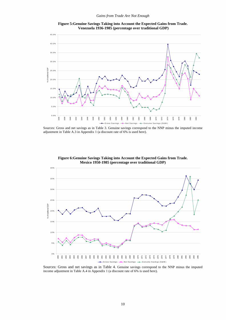
Employing this equation, Tables 1 and 2 present evidence on how much the terms of

trade fluctuations actually affect estimates of national income and contrast these

results with the expected gains from the terms of trade assumed by the imputed

income method. The results are shown as the percentage adjustment in income


14

(NNP). Within each table, Panel a examines the relevant periods by decade

averages, while Panel b divides the years into periods based on broad trends (such

as peak-to-trough movements) in the terms of trade. This second Panel magnifies the

possible effects of the terms of trade on measured income in the case of the actual

effect figures. The first line of each table describes the importance of trade in the

economy. It is evident from this line that the share of exports in Venezuela’s income is

much important than that of Mexico. This is relevant because as Spraos [57] revealed

the effects of the changes in the terms of trade on income are more important the

higher the proportion of income that is derived from exports.

By decades, the adjustment is most significant in the 1970s and the 1980s but with

opposite signs. The figures for the terms of trade adjustment may be interpreted as

follows: if the increase in the terms of trade from 1970 to 1979 is taken into account,

then the recorded national income in 1979 understates the level of Venezuela’s

income by about 7.2 percent. Similarly, the decline in the terms of trade of the 1980s

means that the national income in 1989 overstates the level of Mexico’s income by

about 1 percent.

In looking at broad trends in the terms of trade (Panel b), the adjustment is also

important (about 2 percent) for the period 1943-1957 for Venezuela, and the effects of

the changes in the terms of trade of the oil boom and oil crisis are considerably

magnified for both countries. These findings may lead economic historians to revise,

at the margin, their interpretation of parts of the century. As a consequence of the

terms of trade improvements, it appears that income increased much more than

suggested by conventional estimates of national income during the 1970s. Likewise,

the 1980s saw stronger losses in income than national accounts data suggested

because of the sharp deterioration of the terms of trade during the what it has been

called in Latin-American historiography the ‘lost decade’.


15

Table 1: Terms of Trade Effects on Venezuela's National Income (all figures as percentage of NNP)

Panel a 1936-1939 1940-1949 1950-1959 1960-1969 1970-1979 1980-1985

Share of exports 32.4% 28.0% 32.2% 29.7% 31.2% 27.4%Expected effect 13.5% 17.2% 18.3% 15.4% 23.3% 41.4%Actual effect 0.3% 1.1% 1.3% 0.0% 7.2% -2.5%

Panel b 1936-1942 1943-1957 1958-1972 1973-1981 1982-1985 1936-1985

Share of exports 32.8% 29.4% 29.2% 32.6% 26.1% 30.1%Expected effect 15.2% 17.9% 14.9% 30.3% 43.7% 20.9%Actual effect 0.1% 2.0% -0.3% 9.9% -8.3% 1.7%

Sources: The expected effect on income from expected improvements in the terms of trade corresponds to the second term (Vt(i/(1+i)) of Sefton and Weale’s equation. The actual effect on income from changes in terms of trade calculated using Nicholson’s method defined in equation [3] with data on exports as in Appendix B and terms of trade as in Figure 3. The sources of the NNP are listed in Appendix D.

Table 2: Terms of Trade Effects on Mexico's National Income (all figures as percentage of NNP)

Panel a 1960-1969 1970-1979 1980-1989 1960-1989

Share of exports 6% 5% 14% 8% Expected effect 0.1% 1.8% 26.9% 9.6% Actual effect 0.1% 0.1% -1.0% -0.3%

Panel b 1960-1973 1974-1981 1982-1986 1987-1989

Share of exports 5% 6% 16% 15% Expected effect 0.0% 7.8% 34.6% 17.3% Actual effect 0.0% 0.6% -2.6% 0.6%

Sources: The expected effect corresponds to the second term (Vt(i/(1+i)) of Sefton and Weale’s adjustment. The actual effect on income from changes in terms of trade calculated using Nicholson’s method defined in equation [3] with data on exports as in Appendix B and terms of trade as in Figure 4. The sources of the NNP are listed in Appendix D.


16

All in all, the actual effect on income from the terms of trade is much smaller than the

imputed income for each and every period. This is also true for the whole period: an

actual gain of 1.7 percent contrasts with the expected gain of 20.9 percent for the

period 1936-1985 for Venezuela, and for Mexico an expected gain of 9.6 per cent

contrasts with an actual loss of –0.3 percent for the period 1960-1989. The terms of

trade do not appear to have helped oil producers over the long run as much as some

theoretical models predict. We can now re-calculate the Z indicator taking into

account the effects on income from the actual changes in the terms of trade. Figures

9 and 10 display the results.

Contrary to the results obtained using the expected gains from trade, the additions to

income due to the historical changes in the terms of trade do not suffice to

compensate for the depletion of oil reserves, resulting in the return of the paradox of

negative genuine savings for over 30 years in the case of Venezuela and yet no

observable decline in well-being. The Mexican indicator also improves slightly as a

consequence of the effects of the terms of trade, but it still remains negative for the

early 1980s.

Following Irwin [27] at least two caveats should be noted to this section. First, the

analysis presented here presumes that an increase in the relative price of

exportables, an improvement in the terms of trade, is also an improvement from some

welfare standpoint. Although Krueger et al. [28] established this presumption, simple

connections between the terms of trade and national income or economic welfare

cannot necessarily be drawn. In words of Irwin, ‘a tariff that improves the terms of

trade, for example, may no increase national income if it reduces the volume of trade

excessively.’ Second, the figures for NNP and savings are estimates and their

precision should not be overstated. Thus, the figures presented here should be

considered merely illustrative of the impacts of the terms of trade and depreciation of

natural capital on national income.


17

Figure 9: Genuine Savings Taking into Account the Actual Gains from Trade. Venezuela 1936-1985 (percentage over traditional GDP)

-40 .0%

-30.0%

-20.0%

-10.0%

0.0%

10.0%

20.0%

30.0%

40.0%

50.0%

60.0%

70.0%

1936

1938

1940

1942

1944

1946

1948

1950

1952

1954

1956

1958

1960

1962

1964

1966

1968

1970

1972

1974

1976

1978

1980

1982

1984

% o

f GD

P

G ross Savings N et Savings G enuine Savings (orig ina l) G enuine Savings (ac tual T O T )

Sources: Gross and net savings as in Figure 1. Genuine savings correspond to the NNP (Appendix D) twice adjusted: firstly by the effects of the changes in the terms of trade calculated in Table 1 and secondly the corresponding natural capital depreciation was deducted.

Figure 10: Genuine Savings Taking into Account the Actual Gains from Trade.

Mexico 1950-1985 (percentage over traditional GDP)

-20%

-10%

0%

10%

20%

30%

40%

1960 1961 1962 1963 1964 1965 1966 1967 1968 1969 1970 1971 1972 1973 1974 1975 1976 1977 1978 1979 1980 1981 1982 1983 1984 1985

% o

f tra

ditio

nal G

DP

G ross Savings Net Savings G enuine Saving (standard) Genuine Savings (TOT adj)

Sources: Gross and net savings as in Figure 2. Genuine savings correspond to the NNP as listed in Appendix D twice adjusted: firstly by the effects of the changes in the terms of trade calculated in Table 2 and secondly the corresponding natural capital depreciation was deducted.


18

This paper has explored the first of two theoretical objections to the Z>0 rule: the role

of capital gains arising from improved terms of trade. It has been shown that although

theoretically it can be expected that the gains from improved terms of trade more than

compensate for the cost of depleting oil resources, thus guaranteeing the future

consumption of an oil exporter country, the historical changes in the terms of trade do

not correspond to the theoretical expectations. The historical evolution of the terms of

trade do not suffice to explain why Mexico and in particular Venezuela have enjoyed

non-declining consumption levels despite consuming most of the rents generated by

oil extraction. The terms of trade influenced income, but much less than expected,

being even negative in some instances. The results show that the role of

technological change in sustaining the historical levels of consumption may be

substantial since the terms of trade did not improve in the continuous way needed to

rescue the two economies from declining levels of consumption. This is an important

finding because while gains from trade have now been included in some

environmental accounting models, technological change is left out. As expected by environmental accountants, income differs when natural resources

are included in national accounts. But traditional income estimates do not always

exaggerate income as standard environmental accounting predicts once the effects of

the terms of trade are considered. This should not discourage environmental

accountants for it implies that the misfit between traditional and environmentally

adjusted income is even greater than simple theoretical models predicted. Traditional

measures of income can no longer be considered either a reliable indicator of

sustainable income or the future consumption possibilities of the economy.

These results also have implications for the analysis of the contrasting strategies of

Mexico and Venezuela. It would appear that Venezuela’s pure-resource-exporter

policy was more of a worry for environmental accountants than Mexico’s

conservationist approach. Nevertheless, the fact that Mexico opted for a closed

economy implies that there was a greater need to set aside the rents to replace the

depleted asset than if it had remained an open economy. Only in an open economy

does the possibility of capital gains from the terms of trade on the depleting asset

stock become relevant. In the 1970s, Mexican policy changed at the point when it

would have become even more relatively expensive to remain as a closed economy.

This should not however be taken as support for Venezuelan policies or for those

recommending that little or none of the rent should be reinvested for guaranteeing

future consumption possibilities. The resource exporter can consume today more not

only on account of the expected gains from the terms of trade as we saw, but also

because more of the resource will be available tomorrow at lower costs thanks to


19

technological change. But technological change is double edged. Technological

change can give costs advantages to the competitor producer countries or in the

extreme case it can eliminate the economic value of the reserves, etc, making

obsolete the whole of the natural capital stock. Then not even reinvesting the whole of

the current rent may guarantee the maintenance of the current level of consumption.

The results presented here are initial efforts at estimating indicators and are offered in

the spirit of transparent exchange of research results and thinking. They are intended

to stimulate dialogue and to advance both the methodologies used and the policy

applications of indicators for sustainable development. We learned that with no

technological change and no capital gains from trade, Venezuela would have been off

the sustainability path for over 40 years. The existence of anticipated capital gains for

the most part of the twentieth century allowed the country to avoid the expected

decline in well being expected from a negative savings indicator. The crucial

importance of capital gains/losses in determining the sustainability of resource driven

economies, opens a new item in the empirical research agenda of environmental

accountants

The analysis of different economic strategies and their impact on development and

environmental depletion measures yield new questions for the long-term sustainable

growth debate. Consequently, the results obtained have implications for political

planning over the use of the environment and the use of the recommendations made

by the environmental adjustments.

A final remark applies to all the exercises in this paper. The analyst should bear in

mind that savings are for the most part a residual value calculated from the macro

economic data which sources are in Appendix D, that in the calculation of the

resource rent average and not marginal costs have been used and that most of the

traditional macro indicators used in the calculations are also estimates. Nevertheless,

the overall message of the paper seems robust enough even when the figures

provided are not as precise as desired.


20

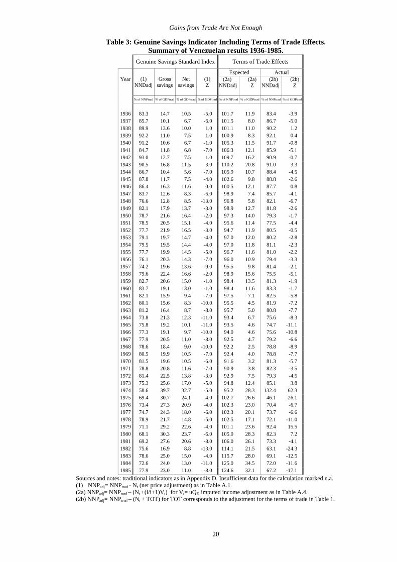
Table 3: Genuine Savings Indicator Including Terms of Trade Effects. Summary of Venezuelan results 1936-1985.

Genuine Savings Standard Index Terms of Trade Effects

Expected Actual Year (2a)

NNDadj(2a)

Z (2b)

NNDadj(2b)

Z

(1) NNDadj

Gross savings

Net savings

(1) Z

% of NNPtrad % of GDPtrad % of GDPtrad % of GDPtrad % of NNPtrad % of GDPtrad % of NNPtrad % of GDPtrad

1936 83.3 14.7 10.5 -5.0 101.7 11.9 83.4 -3.9 1937 85.7 10.1 6.7 -6.0 101.5 8.0 86.7 -5.0 1938 89.9 13.6 10.0 1.0 101.1 11.0 90.2 1.2 1939 92.2 11.0 7.5 1.0 100.9 8.3 92.1 0.4 1940 91.2 10.6 6.7 -1.0 105.3 11.5 91.7 -0.8 1941 84.7 11.8 6.8 -7.0 106.3 12.1 85.9 -5.1 1942 93.0 12.7 7.5 1.0 109.7 16.2 90.9 -0.7 1943 90.5 16.8 11.5 3.0 110.2 20.8 91.0 3.3 1944 86.7 10.4 5.6 -7.0 105.9 10.7 88.4 -4.5 1945 87.8 11.7 7.5 -4.0 102.6 9.8 88.8 -2.6 1946 86.4 16.3 11.6 0.0 100.5 12.1 87.7 0.8 1947 83.7 12.6 8.3 -6.0 98.9 7.4 85.7 -4.1 1948 76.6 12.8 8.5 -13.0 96.8 5.8 82.1 -6.7 1949 82.1 17.9 13.7 -3.0 98.9 12.7 81.8 -2.6 1950 78.7 21.6 16.4 -2.0 97.3 14.0 79.3 -1.7 1951 78.5 20.5 15.1 -4.0 95.6 11.4 77.5 -4.4 1952 77.7 21.9 16.5 -3.0 94.7 11.9 80.5 -0.5 1953 79.1 19.7 14.7 -4.0 97.0 12.0 80.2 -2.8 1954 79.5 19.5 14.4 -4.0 97.0 11.8 81.1 -2.3 1955 77.7 19.9 14.5 -5.0 96.7 11.6 81.0 -2.2 1956 76.1 20.3 14.3 -7.0 96.0 10.9 79.4 -3.3 1957 74.2 19.6 13.6 -9.0 95.5 9.8 81.4 -2.1 1958 79.6 22.4 16.6 -2.0 98.9 15.6 75.5 -5.1 1959 82.7 20.6 15.0 -1.0 98.4 13.5 81.3 -1.9 1960 83.7 19.1 13.0 -1.0 98.4 11.6 83.3 -1.7 1961 82.1 15.9 9.4 -7.0 97.5 7.1 82.5 -5.8 1962 80.1 15.6 8.3 -10.0 95.5 4.5 81.9 -7.2 1963 81.2 16.4 8.7 -8.0 95.7 5.0 80.8 -7.7 1964 73.8 21.3 12.3 -11.0 93.4 6.7 75.6 -8.3 1965 75.8 19.2 10.1 -11.0 93.5 4.6 74.7 -11.1 1966 77.3 19.1 9.7 -10.0 94.0 4.6 75.6 -10.8 1967 77.9 20.5 11.0 -8.0 92.5 4.7 79.2 -6.6 1968 78.6 18.4 9.0 -10.0 92.2 2.5 78.8 -8.9 1969 80.5 19.9 10.5 -7.0 92.4 4.0 78.8 -7.7 1970 81.5 19.6 10.5 -6.0 91.6 3.2 81.3 -5.7 1971 78.8 20.8 11.6 -7.0 90.9 3.8 82.3 -3.5 1972 81.4 22.5 13.8 -3.0 92.9 7.5 79.3 -4.5 1973 75.3 25.6 17.0 -5.0 94.8 12.4 85.1 3.8 1974 58.6 39.7 32.7 -5.0 95.2 28.3 132.4 62.3 1975 69.4 30.7 24.1 -4.0 102.7 26.6 46.1 -26.1 1976 73.4 27.3 20.9 -4.0 102.3 23.0 70.4 -6.7 1977 74.7 24.3 18.0 -6.0 102.3 20.1 73.7 -6.6 1978 78.9 21.7 14.8 -5.0 102.5 17.1 72.1 -11.0 1979 71.1 29.2 22.6 -4.0 101.1 23.6 92.4 15.5 1980 68.1 30.3 23.7 -6.0 105.0 28.3 82.3 7.2 1981 69.2 27.6 20.6 -8.0 106.0 26.1 73.3 -4.1 1982 75.6 16.9 8.8 -13.0 114.1 21.5 63.1 -24.3 1983 78.6 25.0 15.0 -4.0 115.7 28.0 69.1 -12.5 1984 72.6 24.0 13.0 -11.0 125.0 34.5 72.0 -11.6 1985 77.9 23.0 11.0 -8.0 124.6 32.1 67.2 -17.1

Sources and notes: traditional indicators as in Appendix D. Insufficient data for the calculation marked n.a. (1) NNPadj= NNPtrad - Nt (net price adjustment) as in Table A.1. (2a) NNPadj= NNPtrad – (Nt +(i/i+1)Vt) for Vt= uQE imputed income adjustment as in Table A.4. (2b) NNPadj= NNPtrad – (Nt + TOT) for TOT corresponds to the adjustment for the terms of trade in Table 1.


21

Table 4: Genuine Savings Indicator Including Terms of Trade Effects.

Summary of Mexican results 1950-1985.

Genuine Savings Standard Index Terms of Trade Effects

Expected Actual Year

(1) NNDadj

Gross savings

Net savings

(1) Z (2a)

NNDadj(2a)

Z (2b) NNDadj

(2b) Z

% of NNPtrad % of GDPtrad % of GDPtrad % of GDPtrad % of NNPtrad % of GDPtrad % of NNPtrad % of GDPtrad

1950 98.0 20.3 7.1 5.5 98.3 5.7 n.a n.a 1951 98.2 18.4 5.4 3.9 98.4 4.0 n.a n.a 1952 98.2 20.6 7.4 5.9 98.6 6.2 n.a n.a 1953 98.8 18.6 5.3 4.3 98.8 4.3 n.a n.a 1954 98.5 20.4 7.6 6.4 98.6 6.4 n.a n.a 1955 98.7 21.4 8.8 7.8 98.8 7.8 n.a n.a 1956 98.8 21.5 8.7 7.8 98.9 7.8 n.a n.a 1957 98.6 19.8 7.0 5.9 98.7 5.9 n.a n.a 1958 98.9 19.0 6.3 5.5 98.9 5.4 n.a n.a 1959 99.2 19.7 6.9 6.3 99.2 6.2 n.a n.a 1960 99.5 21.2 6.9 6.6 99.5 6.5 99.5 6.5 1961 99.1 17.5 4.5 3.9 99.2 3.8 99.2 3.8 1962 99.0 17.4 5.1 4.4 99.1 4.4 98.9 4.2 1963 99.1 17.6 4.4 3.7 99.2 3.7 98.7 3.3 1964 99.3 15.7 3.6 3.1 99.3 3.1 99.3 3.0 1965 99.4 15.5 3.3 2.9 99.4 2.9 99.4 2.8 1966 99.5 16.9 4.8 4.5 99.6 4.5 99.5 4.4 1967 99.6 18.7 6.6 6.4 99.6 6.3 99.5 6.1 1968 99.7 18.7 6.5 6.3 99.7 6.2 99.6 6.2 1969 99.7 26.0 13.2 13.0 99.7 12.9 99.8 13.0 1970 99.7 25.8 14.4 14.2 99.8 14.1 99.6 14.0 1971 99.6 27.5 12.8 12.5 99.6 12.4 99.6 12.4 1972 99.6 27.4 13.1 12.8 99.6 12.7 99.7 12.8 1973 99.3 27.0 13.9 13.3 99.3 13.2 99.3 13.2 1974 97.1 25.7 14.3 11.7 97.2 11.7 96.8 11.3 1975 96.9 24.3 14.1 11.3 97.2 11.5 96.9 11.2 1976 96.0 22.4 13.4 9.9 96.7 10.4 95.8 9.5 1977 94.1 22.3 15.1 9.8 95.7 11.0 94.7 10.2 1978 94.3 23.5 15.8 10.8 100.6 16.4 94.1 10.4 1979 92.5 23.6 15.9 9.3 101.9 17.7 91.7 8.3 1980 86.8 26.5 14.2 2.4 106.9 19.7 83.5 -1.8 1981 86.2 29.6 13.4 1.1 110.0 21.9 85.7 -0.3 1982 77.3 36.3 13.1 -6.5 116.1 27.3 79.0 -5.3 1983 69.9 32.6 13.1 -12.7 126.8 36.0 77.8 -5.9 1984 90.5 29.9 11.3 3.3 108.2 18.4 90.5 3.2 1985 79.8 34.4 11.4 -5.7 116.4 25.1 80.4 -5.4

Sources and notes: traditional indicators as in Appendix D. Insufficient data for the calculation marked n.a. (1) NNPadj= NNPtrad – Nt , net price adjustment as in Table A.2. (2a) NNPadj= NNPtrad – (Nt +(i/i+1)Vt) for Vt= uQE , imputed income adjustment as in Table A.4. (2b) NNPadj= NNPtrad – (Nt + TOT) for TOT corresponds to the adjustment for the terms of trade in Table 2.


22

APPENDIX 1

Table A.1: Venezuelan resource rent through time, 1920-1985 Aggregated rent, N Rent per unit, u Year Mll. Blv. Bolivars As % of price per barrel

1920 -4.8 -9.5 1921 -5.1 -3.7 1922 -3.7 -1.7 1923 4.4 1.0 13% 1924 31.5 3.5 39% 1925 98.4 4.9 54% 1926 206.0 5.8 62% 1927 218.4 3.6 56% 1928 375.2 3.5 67% 1929 581.7 4.3 71% 1930 608.2 4.5 73% 1931 332.1 2.8 66% 1932 496.3 4.3 77% 1933 176.2 1.5 54% 1934 303.6 2.2 67% 1935 332.7 2.2 68% 1936 362.7 2.3 68% 1937 384.5 2.1 65% 1938 293.0 1.6 54% 1939 238.1 1.2 47% 1940 257.5 1.4 49% 1941 426.7 1.9 62% 1942 188.2 1.3 41% 1943 295.0 1.6 52% 1944 513.8 2.0 62% 1945 648.2 2.0 61% 1946 905.6 2.3 60% 1947 1,502.3 3.5 64% 1948 2,556.7 5.2 70% 1949 2,200.9 4.6 66% 1950 2,561.0 4.7 72% 1951 2,754.2 4.4 72% 1952 3,123.1 4.7 72% 1953 3,284.9 5.1 72% 1954 3,593.7 5.2 73% 1955 4,316.1 5.5 76% 1956 4,956.6 5.5 76% 1957 6,277.0 6.2 76% 1958 5,261.6 5.5 72% 1959 4,789.4 4.7 69% 1960 4,572.1 4.4 67% 1961 4,907.0 4.6 70% 1962 5,592.0 4.8 75% 1963 5,550.4 4.7 75% 1964 8,653.4 7.0 82% 1965 8,551.9 6.7 82% 1966 8,295.8 6.7 82% 1967 8,671.7 6.7 82% 1968 8,990.5 6.8 83% 1969 8,663.9 6.6 83% 1970 9,088.4 6.7 83% 1971 11,385.9 8.8 86% 1972 11,143.4 9.5 87% 1973 17,178.3 14.0 90% 1974 45,686.0 42.1 95% 1975 36,840.9 43.0 93% 1976 37,409.2 44.6 94% 1977 41,662.7 51.1 95% 1978 37,662.5 47.7 93% 1979 62,337.5 72.5 94% 1980 83,690.1 105.5 93% 1981 90,320.7 117.5 92% 1982 72,278.0 104.6 89% 1983 60,657.9 92.3 85% 1984 93,405.6 141.7 89% 1985 82,187.4 134.1 86% Sources and notes: Nt= pq-rk-cl, that is the resource rent is the residual to the owner after discounting capital and labour costs from the gross revenue. Elaborated from the data in Appendixes A, F, G and H. A return of 15 per cent on capital invested in the oil sector was allowed in this calculation. Several alternative calculations on the return to capital were tried and do not convey substantial changes to the final results. These can be found in Rubio [52].


23

Table A.2: Mexican resource rent through time, 1927-1987 Aggregated rent, N Rent per unit, u year Mill. pesos pesos As percentage of price

per barrel 1921 1922 1923 1924 1925 1926 1927 126,45 1,97 80% 1928 73,62 1,47 72% 1929 65,60 1,47 71% 1930 61,55 1,56 76% 1931 55,52 1,68 72% 1932 49,63 1,51 66% 1933 57,86 1,87 70% 1934 109,04 2,86 86% 1935 113.97 2.83 83% 1936 104.53 2.55 77% 1937 192.95 4.12 84% 1938 133.20 3.46 73% 1939 107.63 2.51 59% 1940 81.55 1.85 51% 1941 83.32 1.94 55% 1942 61.64 1.77 46% 1943 63.35 1.80 44% 1944 43.81 1.15 29% 1945 26.51 0.61 16% 1946 69.53 1.41 27% 1947 95.60 1.70 34% 1948 306.36 5.24 59% 1949 412.22 6.77 62% 1950 737.08 10.18 74% 1951 854.98 11.06 72% 1952 967.04 12.51 73% 1953 656.61 9.07 63% 1954 957.91 11.45 66% 1955 997.48 11.16 63% 1956 1,081.69 11.93 63% 1957 1,395.71 15.81 65% 1958 1,228.90 13.14 22% 1959 987.68 10.25 53% 1960 664.06 6.70 41% 1961 1,342.55 12.57 59% 1962 1,548.65 13.85 60% 1963 1,507.72 13.13 58% 1964 1,474.52 12.76 55% 1965 1,354.98 11.49 49% 1966 1,212.38 10.01 43% 1967 1,185.42 8.91 38% 1968 981.42 6.89 30% 1969 1,121.84 7.49 33% 1970 1,050.03 6.70 29% 1971 1,745.92 11.20 38% 1972 2,109.21 13.07 41% 1973 4,703.35 28.52 62% 1974 24,029.17 114.50 87% 1975 32,123.24 122.80 88% 1976 50,602.45 172.64 91% 1977 100,964.59 281.95 93% 1978 122,561.50 276.91 92% 1979 209,874.85 390.88 93% 1980 517,399.55 730.18 96% 1981 740,845.46 877.87 96% 1982 1,881,754.29 1,877.18 97% 1983 4,429,150.09 4,552.49 99% 1984 2,331,022.40 2,378.98 96% 1985 8,148,324.36 8,486.66 98% 1986 7,847,933.75 8,856.60 97% 1987 23,235,250.45 25,056.37 97%

Sources and notes: Nt= pq-rk-cl, that is the resource rent is the residual to the owner after discounting capital and labour costs from the gross revenue. Elaborated from the data in Appendixes A, F, G and H. A return of 6 per cent on capital invested in the oil sector was allowed in this calculation. Several alternative calculations on the return to capital were tried and do not convey substantial changes to the final results. These can be found in Rubio [52]


24

Table A.3: Imputed value to the stock targeted for exports for Venezuela 1921-1985, Sefton and Weale Method. (negative figures in parentheses)

Year Vt=utQE -Nt+Vt(i/1+i) i=3% i=6% i=15%

1921 (149.08) 0.77 (3.33) (14.34)1922 (140.54) (0.37) (4.23) (14.60)1923 202.65 1.51 7.08 22.05 1924 1,724.67 18.71 66.10 193.43 1925 2,446.21 (27.15) 40.07 220.67 1926 4,194.66 (83.80) 31.46 341.15 1927 3,464.23 (117.50) (22.31) 233.45 1928 4,246.87 (251.46) (134.76) 178.79 1929 3,990.64 (465.45) (355.79) (61.16)1930 5,328.35 (452.97) (306.56) 86.84 1931 3,540.41 (228.97) (131.69) 129.70 1932 6,233.77 (314.70) (143.41) 316.84 1933 2,547.60 (101.96) (31.96) 156.13 1934 5,543.86 (142.09) 10.25 419.56 1935 6,429.00 (145.49) 31.16 505.82 1936 7,050.14 (157.37) 36.35 556.87 1937 7,519.11 (165.54) 41.07 596.21 1938 5,761.94 (125.19) 33.14 458.55 1939 4,709.35 (100.96) 28.44 376.14 1940 7,263.64 (45.95) 153.63 689.92 1941 10,644.62 (116.71) 175.78 961.68 1942 7,928.94 42.75 260.62 846.02 1943 10,791.19 19.30 315.82 1,112.54 1944 13,136.11 (131.17) 229.78 1,199.63 1945 13,911.06 (243.06) 139.18 1,166.25 1946 16,569.10 (423.00) 32.28 1,255.59 1947 24,675.17 (783.58) (105.56) 1,716.23 1948 39,011.97 (1,420.46) (348.51) 2,531.79 1949 36,461.71 (1,138.86) (136.98) 2,555.02 1950 39,511.32 (1,410.22) (324.55) 2,592.61 1951 38,786.71 (1,624.50) (558.74) 2,304.93 1952 42,138.92 (1,895.72) (737.84) 2,373.31 1953 49,563.93 (1,841.30) (479.40) 3,179.95 1954 54,155.41 (2,016.35) (528.29) 3,470.06 1955 64,802.85 (2,428.62) (648.00) 4,136.46 1956 73,072.17 (2,828.30) (820.46) 4,574.54 1957 91,598.38 (3,609.07) (1,092.18) 5,670.63 1958 87,861.97 (2,702.49) (288.26) 6,198.68 1959 76,644.19 (2,557.04) (451.05) 5,207.67 1960 73,001.87 (2,445.86) (439.95) 4,949.85 1961 74,373.97 (2,740.73) (697.11) 4,793.99 1962 76,710.32 (3,357.75) (1,249.94) 4,413.67 1963 75,832.04 (3,341.74) (1,258.06) 4,340.69 1964 114,054.70 (5,331.45) (2,197.51) 6,223.26 1965 110,532.69 (5,332.48) (2,295.31) 5,865.43 1966 107,730.95 (5,157.97) (2,197.78) 5,756.10 1967 101,568.39 (5,713.44) (2,922.59) 4,576.31 1968 101,106.42 (6,045.65) (3,267.49) 4,197.30 1969 93,133.68 (5,951.31) (3,392.23) 3,483.93 1970 87,447.84 (6,541.37) (4,138.52) 2,317.85 1971 115,111.21 (8,033.12) (4,870.14) 3,628.64 1972 121,395.17 (7,607.67) (4,272.03) 4,690.70 1973 239,467.92 (10,203.47) (3,623.47) 14,056.68 1974 713,399.88 (24,907.35) (5,304.86) 47,366.18 1975 708,383.56 (16,208.35) 3,256.30 55,556.97 1976 717,854.94 (16,500.85) 3,224.05 56,224.00 1977 802,217.38 (18,297.18) 3,745.80 62,974.32 1978 742,623.13 (16,032.70) 4,372.77 59,201.38 1979 1,144,123.63 (29,013.55) 2,424.18 86,895.98 1980 1,709,050.38 (33,911.98) 13,048.55 139,229.47 1981 1,906,609.75 (34,788.37) 17,600.62 158,367.53 1982 2,014,999.75 (13,588.65) 41,778.63 190,548.09 1983 1,859,640.38 (6,493.59) 44,604.80 181,903.91 1984 3,153,399.75 (1,559.03) 85,088.70 317,907.38 1985 3,065,309.50 7,093.42 91,320.66 317,635.53

Nt as in Table A.1 QE is the stock targeted for exports ‘assuming the ratio of the domestic utilisation of the resource to foreign utilisation remains constant’. Data derived from the data in Appendix A.


25

Table A.4: Imputed value to the stock targeted for exports. Mexico 1935-1985

Sefton and Weale Method. (negative figures in parentheses) Year Vt=utQE -Nt+Vt(i/1+i)

i=3% i=6% i=15% 1935 1,997.75 (55.78) (0.89) 146.61 1936 1,657.15 (56.27) (10.73) 111.62 1937 2,045.39 (133.37) (77.17) 73.84 1938 945.37 (105.67) (79.69) (9.89) 1939 911.49 (81.09) (56.04) 11.26 1940 689.32 (61.47) (42.53) 8.36 1941 402.57 (71.60) (60.54) (30.81) 1942 170.28 (56.68) (52.00) (39.43) 1943 52.46 (61.83) (60.38) (56.51) 1944 27.18 (43.02) (42.27) (40.26) 1945 29.18 (25.66) (24.86) (22.71) 1946 101.56 (66.57) (63.78) (56.29) 1947 114.33 (92.27) (89.13) (80.69) 1948 1,198.39 (271.46) (238.53) (150.05) 1949 975.66 (383.80) (356.99) (284.96) 1950 2,319.55 (669.53) (605.79) (434.53) 1951 1,686.54 (805.86) (759.51) (635.00) 1952 3,766.17 (857.34) (753.86) (475.80) 1953 876.51 (631.08) (607.00) (542.28) 1954 1,372.45 (917.93) (880.22) (778.89) 1955 1,547.23 (952.41) (909.90) (795.67) 1956 1,943.57 (1,025.08) (971.67) (828.18) 1957 1,419.20 (1,354.38) (1,315.38) (1,210.60) 1958 110.97 (1,225.67) (1,222.62) (1,214.43) 1959 33.28 (986.72) (985.80) (983.34) 1960 228.80 (657.39) (651.10) (634.21) 1961 2,608.93 (1,266.56) (1,194.87) (1,002.25) 1962 2,930.71 (1,463.29) (1,382.77) (1,166.39) 1963 2,646.11 (1,430.65) (1,357.94) (1,162.57) 1964 2,607.30 (1,398.58) (1,326.94) (1,134.44) 1965 2,071.58 (1,294.64) (1,237.72) (1,084.77) 1966 2,566.76 (1,137.62) (1,067.09) (877.59) 1967 2,081.27 (1,124.80) (1,067.61) (913.95) 1968 1,516.93 (937.23) (895.55) (783.56) 1969 1,574.04 (1,076.00) (1,032.75) (916.53) 1970 2,375.19 (980.85) (915.58) (740.22) 1971 1,696.81 (1,696.50) (1,649.88) (1,524.60) 1972 1,244.49 (2,072.96) (2,038.77) (1,946.89) 1973 2,554.10 (4,628.96) (4,558.78) (4,370.20) 1974 10,945.76 (23,710.37) (23,409.60) (22,601.46) 1975 65,245.06 (30,222.89) (28,430.12) (23,613.01) 1976 151,312.21 (46,195.30) (42,037.61) (30,866.07) 1977 475,758.31 (87,107.55) (74,034.88) (38,909.16) 1978 2,395,112.37 (52,800.94) 13,010.91 189,844.47 1979 4,648,334.08 (74,486.48) 53,238.39 396,429.56 1980 13,943,776.20 (111,270.19) 271,870.78 1,301,353.75 1981 22,541,948.51 (84,283.81) 535,113.94 2,199,408.50 1982 56,838,225.94 (226,271.88) 1,335,503.75 5,531,927.00 1983 147,849,366.55 (122,857.50) 3,939,682.00 14,855,550.00 1984 76,856,905.87 (92,471.75) 2,019,368.50 7,693,791.50 1985 260,638,189.67 (556,921.00) 6,604,780.50 25,847,960.00 1986 259,935,103.18 (277,008.50) 6,865,374.00 26,056,646.00 1987 726,356,555.59 (2,079,234.00) 17,879,274.00 71,506,912.00 1988 918,474,382.47 (3,278,902.00) 21,958,532.00 89,770,424.00 1989 822,735,404.02 (17,498,832.00) 5,107,928.00 65,851,312.00

Ntt as in Table A.2 QE is the stock targeted for exports ‘assuming the ratio of the domestic utilisation of the resource to foreign utilisation remains constant’. Data derived from the data in Appendix A.


26

APPENDIX 2

The adjustment proposed by Sefton and Weale to conventional income for the use of non-

renewable resources can be expressed as follows once the rate of interest is held constant

over time:1

( ) ∫ ∫∞

⎟⎟⎠

⎞⎜⎜⎝

⎛−++−=

0 0221 exp)0()0()0( dtrdsrRRRsNNPNNP

t

cw τ [app-1]

NNPw and NNPc denote the welfare income and the conventional expenditure estimate of

national income respectively. The rest of their nomenclature is as follows: s represents the per

unit price of the resource net of costs; R1 the amount of the resource used domestically, R2 the

amount of the resource exported and r is the rate of interest. As derived from the work of

Weitzman [65], in the absence of natural resource, the conventional income equals the welfare

income.

According to Sefton and Weale ‘the term –s(0)(R1(0)+R2(0)) is Hartwick’s adjustment for the

extraction of exhaustible resources in a closed economy’. Indeed, translating into our own

notation we can write this term as u(q1+q2)= Nt, that is the per unit rent times the amount

produced in the year. The remainder of the expression adds up to an imputed income on the

stock of the resource targeted for export. Both terms together constitute the adjustment term

proposed by Sefton and Weale.

They argue that a resource exporter ‘can enjoy a level of positive consumption, because even

though the country deplete its resource stock, the value of the remaining stock increases in

value’. This, they say, can be illustrated clearly from the expression above. If the resource

producing country exports all its oil, R1=0, then they claim the adjustment term becomes

∫ ∫∞

=−+−0 0

22 0)exp(t

dtrdrsRsR τ [app-2]

So they conclude that ‘in this case welfare income equals the conventional measure of NNP

so there is effectively no adjustment required’. But how can the adjustment term be equal to

zero? Take the alternative form of expressing the adjustment term also provided by Sefton and

Weale. Define SE(t) as the amount of the present stock of the resource earmarked for export,

so that

∫∞

=tE dRtS ττ )()( 2 [app-3]

1 This equation is a simplification of equation (46) in Sefton and Weale p.40, which originally reads:

( ) ∫ ∫ ∫∫∫ ∫∞ ∞ ∞•∞

⎟⎟⎠

⎞⎜⎜⎝

⎛−+⎟⎟

⎠

⎞⎜⎜⎝

⎛−++−+−++=⎟⎟

⎠

⎞⎜⎜⎝

⎛−

0 0 01

022112111

0 01 expexp)0()0()0()0()0())0()0()0(()0()0()0(exp dtrdHrdtrdsrRRRsHrTRsIqCdtrdrC

tt

τττ

The left-hand side is welfare income. The four first terms in the right-hand side are the principal elements of the standard NNP: consumption, investment, the balance of trade and net property income. The last term corresponds to the imputed income due to future interest rate changes and it is equal to zero if the interest rate is not expected to change over time.


27

Making use of Hotelling’s rule, which implies that the price of the resource net of extraction

costs increases over time at the rate of interest (this is the continuous version of the discrete

equation app4 above), thus

⎟⎠⎞⎜

⎝⎛= ∫

trdss

0exp)0( τ [app-4]

then the adjustment term can be expressed as:

ESsrsR )0()0(2 +− [app-5]

This is simply the result of taking the solution of the integral side of the adjustment term from

equation (48) in Sefton and Weale (assuming real interest remains constant). Since R1=0, all

of the resource is exported and SE equals the whole stock of the resource available S(0).

Observe that for adjustment term to become zero (so that no adjustment is required), the only

possibility is that the ratio of production to reserves must equal the exogenous rate of interest

(R2/S(0)=r), otherwise ‘the adjustment could be positive or negative at any point along the

optimal path’.

A closer look at the adjustment proposed by Sefton and Weale reveals that, if the whole of the

resource is exported, their adjustment is conceptually equivalent to the adjustment framed by

the Fundamental Equation of Asset Equilibrium. Translated into our notation, s is the per unit

price of the resource ut; R2 is the quantity extracted for exports q2 (understanding that total

production equals production for domestic use plus production for exports, qt=q1+q2); Q was

the notation used for the reserves or total stock S(0); using discrete instead of continuous time

formulation, so that the interest rate is i. If all the production is exported the adjustment

proposed by Sefton and Weale becomes:

tttt Qui

iqu)1( +

+− [app-6]

the first term is simply Nt, and we know that utQ is the value of the resource Vt according to

the Hotelling Valuation Principle (HVP), substituting

tt Vi

iN)1( +

+− [app-7]

The adjustment proposed by Sefton and Weale is precisely the change in value of the asset, if

the country exports all of its production, the per unit rents increase following Hotelling’s rule

and the interest rate does not change over time. In a closed economy model, where the

country exports none of its resources and the rate of interest is constant, the adjustment is

identical to the net price, -Nt, because there will be no gains from trade, thus Vt is nil. For a

lengthier description and the calculation of the values presented above see Chapters 2 and 5

in Rubio [52].


28

DATA APPENDICES BY COUNTRY

APPENDIX A: Production and consumption of oil

Venezuela: 1920-1990:Baptista [9], cuadro B-5. México: 1901-1992: México [35] cuadro 11.1, p.559.

APPENDIX B: Exports

Venezuela Total exports and oil exports: • 1911-1963: Venezuela [60], p.1049. From 1911 to 1917, 'oil exports' refer to asphalt

exports. • 1956-1967: Venezuela [61]. p.372, (overlapping years coincide with the previous source). • 1965-1975: PODE for the years 1970, 1973 and 1975, p. 11 in all cases; (overlapping

years coincide). From 1967 to 1975 there are some disagreements in the official published data over the value of oil exports due to different valuation (reference prices, tax prices, market prices)

• 1976-1985: PODE , 1985, pp.1 and 13. Mexico Total exports • 1901-1990 (in dollars in the original): México [35], p. 799-800. Oil exports • 1911-1936: México [30] p.21 (converted here from volume to value by multiplying the

former by the prices shown in Appendix F). • 1937: Haber et al. [18]. • 1938-1939: Pemex [47], p.47. • 1940-1974: Banco Nacional de Comercio Exterior [7]; (there were no exports between

1967 and 1973). • 1974-1988: Pemex [50], p.121.


29

APPENDIX D

Macroeconomic indicators Venezuela

Total GDP:

• 1920-1989: base series at constant prices of 1968 from Baptista [8], pp.35-36 reflated by the corresponding deflator for GDP from the same source, pp.300-301.

NDP: • 1920-1989: Calculated subtracting from the GDP the consumption of fixed

capital at current prices found in Baptista [8], cuadro IV, p.48. Mexico Total GDP: • 1901-1970 & 1990: México [35], p.401-402, cuadro 8.1. • 1987-1988, México [39], p.569, cuadro, 4.11. • 1971-1987: México [32], p.318. NDP/NNP (national income figures): • 1929-1940: (National income) Sáenz [53] p.32. • 1939-1960: (Net National income) Banco de México [5], p.73 (only used until 1950). • 1939-1968: (Net national income used only from 1950 to 1960), Nacional Financiera[40],

table 2.3 ), ultimate source is Banco de México. • 1950-1978: NDP equals the GDP from the sources above minus the consumption of

fixed capital calculated from Hofman series (see next heading below). • 1979-1981: (NNP) México [38], p.26. • 1980-1988: (NNP) Nacional Financiera[41] 1990, p146-147. • 1989-1992: (NNP) México [36], p.33. In order to obtain a complete data series for NDP, its series for the period 1979-1992 were calculated by subtracting the consumption of fixed capital from the GDP. The results are compatible with the NNP official series just referenced. Consumption of fixed capital: • The years pre-1960 calculated as the difference between the GDP and the national

income, (see above). • 1960-1978: the difference between the gross stock and the net stock of capital estimated

by Hofman [25], Table E.20 reflated to current prices by the corresponding average price indices for buildings/infrastructure and machinery and equipment by México [35], pp.966-967.

• 1977-1980: México [38], p.309. • 1980-1988: Nacional Financiera[41], p146-147 • 1984-1987: México [34], p.559. • 1988-1989: México [33], p.569. • 1990-1992: México [36], p.33.


30

APPENDIX E: Oil reserves

Venezuela Oil Reserves

• 1919, 1924, 1929, 1934 and 1939: [29], p.166.

• 1925 and 1935: United Nations [58], p.59.

• 1944-1970: Banco Central de Venezuela [3], p114.

• 1968-1976: Banco Central de Venezuela [4], p. 65 (data back to 1944; overlapping years coincide with the previous source).

• 1944-1985, PODE 1985, published the whole series.

At least until 1967, Venezuelan reserves included condensed materials. In 1982, the reserves of the Orinoco river in Amazonia were also included in the proven reserves despite the technical difficulties involved in their potential exploitation. From 1970 onwards, there are some important discrepancies between the figures published by the national offices and independent sources. These discrepancies obliged OPEC to publish two different sets of data for member countries,1970-1979 data available in the [44], p. 148. Mexico Oil reserves

• 1918: Pemex [49] • 1938-1992: México [35] p.536.

For Mexico, reservoirs seems to include gas along with oil and therefore, the production of natural gas –converted into oil equivalents- were included included at the time of calculating the reserves/production (R/P) ratio. Yet the average of BP [11] separate estimates for oil and gas (over 40 years for oil and above 70 years for gas in 1985) coincides with the figures presented here. The fact that our calculation is consistent with the R/P described by Sordo [56], pp. 102-103 for the history of Pemex provides some reassurance about its reliability.

APPENDIX F:

Oil prices

Venezuela

Oil prices: 1 921-1991: (in dollars per barrel in the original) Baptista [8]

Exchange rate (bolivar/US dollar):

• up to 1938: Venezuela [59], pp.417-420.

• 1939-1963: Venezuela [60], p.1046. • 1963-1985: PODE, 1985, p.151 Mexico Oil prices series knowing volumes and values produced and/or exported, oil prices were inferred from the following sources: • 1901-1923: México [31],p. 28. • 1923-1935: México [30], p.21. • 1938-1939: Pemex [48], p.17. • 1940-1973: Banco Nacional de Comercio Exterior [7] and Banco Nacional de Comercio

Exterior [6] • Prices 1975-1985: BP [10] p.14. Official Government selling prices on the first of January

and July each year (average taken) for the Isthmus crude.


31

APPENDIX G Costs in the oil industry

Venezuela Labour force: • 1921-1990 Baptista [9], cuadro B-5.

Wages in oil industry: • 1921-1990 Baptista [8], pp.139-141. Mexico Labour cost sources are as follow: • 1934-1936: México [37], pp.477-510. • 1937 Pemex [47]. • 1938-1992 México [35], p.573.

APPENDIX H

Capital Investment in the oil industry Venezuela Capital Investment in the Oil industry

• 1920-1946: Baptista [8], cuadro V-30, allocating 60 percent of total investment to the production branch of the industry.

• 1947-1961: Net capital investment in fixed assets in the production branch of the oil industry, Venezuela [62], p.24

• 1960-1970: Net capital investment in fixed assets in the production branch of the industry calculated from data in total net capital investment in fixed assets multiplied by the corresponding percentage of the production branch of the industry, PODE, 1970, p.142.

• 1964-1974: same procedure over data in PODE, 1974, p.13ff.

• 1975-1985: same procedure over data in PODE, 1985, p. 131 Overlapping data coincident, otherwise the most recent source was used.

Mexico

Capital Investment in the Oil Industry

• 1924: Dept. Estadística Nacional, as quoted in Gordon [16], p.53. • 1935: México [37], cuadros 145-160. • 1938-1979: México [35], p. 574. • 1960-1985: Pemex [50]


32

1. G. B. Asheim, Hartwick's rule in open economics, Canadian Journal of Economics (1986), 86, 395-402.

2. G. B. Asheim, Capital gains and net national product in open economies, Journal of Public Economics (1996), 59, 419-434.

3. Banco Central de Venezuela, La economía venezolana en los últimos treinta años, Caracas (1971).

4. Banco Central de Venezuela, La economía venezolana en los últimos treinta cinco años, Caracas (1978).

5. Banco de México, Informe anual, México D.F. (1960).

6. Banco Nacional de Comercio Exterior S.A., 6 años en el comercio exterior de México, México D.F. (1964).

7. Banco Nacional de Comercio Exterior S.A., Comercio Exterior de México, Editorial Cultura, México D.F. (Volumes for the period 1948-1973).

8. A. Baptista, Bases Cuantitativas de la Economía Venezolana, 1830-1989, Caracas (1991).

9. A. Baptista, Bases cuantitativas de la economía Venezolana. 1830-1995 (and data disk), Fundacion Polar, Caracas (1997).

10. British Petroleum, BP Statistical Review of World Energy, 1987, British Petrolum Company (1988).

11. British Petroleum, BP Statistical Review of World Energy, British Petrolum Company (yearly).

12. F. Coronil, The magical state: Nature, money, and modernity in Venezuela, University of Chicago Press, Chicago and London (1997).

13. P. Dasgupta and G. Heal, Economic Theory and Exhaustible Resources, Cambridge University Press, Cambridge (1979).

14. W. Easterly and M. Sewadeh, Global Development Network Growth Database, World Bank (2002).

15. L. W. Goodman, J. Mendelson Forman, M. Naim, J. S. Tulchin and G. Bland Eds., The lessons of the Venezuelan experience, Washington D.C. (1995).

16. W. C. Gordon, The Expropriation of Foreign-Owned Property in Mexico, Amercian Council of Public Affairs, Washington D.C (1941).

17. P. Gutman, The Measurement of Terms of Trade Effects, Review of Income and Wealth (1981), 27, 433-453.

18. S. H. Haber, N. Mauer and A. Razo, When Institutions do not Matter: The Rise and Decline of the Mexican Oil Industry, Paper presented at the Economic History Seminar at UC Berkeley, September 2001 (no published).

19. K. Hamada and K. Iwata, National Income, Terms of Trade and Economic Welfare, The Economic Journal (1984), 94, 752-771.

20. J. M. Hartwick, Intergenerational Equity and the Investing of Rents from Exhaustible Resources, American Economic Review (1977), 67, 972-974.

21. J. M. Hartwick, Natural resources, national accounting and economic depreciation, Journal of Public Economics (1990), 291-304.

22. J. M. Hartwick, Sustainability and constant consumption paths in open economies with exhaustible resources, Review of International Economics (1996), 3, 275-283.

23. J. R. Hicks, Value and Capital: An inquiry into some Fundamental Principles of Economic Theory, Oxford University Press, Oxford, UK (1946).


33

24. A. A. Hofman and N. Mulder, The Comparative Productivity Performance of Brazil and Mexico, 1950-1994, in "Latin America and the World Economy since 1800" (J. H. Coatsworth and A. Taylor, Eds.), Cambridge, MA (1998).

25. A. A. Hofman, The Economic Development of Latin America in the Twentieth Century, Cheltenham, UK (2000).

26. International Bank for Reconstruction and Development (IBRD), The Economic Development of Venezuela, Baltimore (1961).

27. D. Irwin, Terms of Trade and Economic Growth in Nineteenth Century Britain, Bulletin of Economic Research (1991), 43, 93-101.

28. A. O. Krueger and H. Sonnenschein, The Terms of Trade, the Gains from Trade, and Price Divergence, International Economic Review, 8, 121-127.

29. A. R. Martínez, El papel de la explotación petrolera en el proceso de modernización de la sociedad venezolana y la perspectiva inmediata, in "Hacia la Venezuela Post-petrolera [conference sponsored by la Academia Nacional de las Ciencias Económicas in 1985]" (F. Mieres, Ed.), Academia Nacional de Economía, Caracas (1989).

30. México, Government of, Estadística Petrolera, Revista de Industria. Revista Mensual (1937 December), 1, 21.

31. México. Departamento de la Estadística Nacional, El progreso económico de México. Un estudio económico estadístico, Republica Mexicana, México D.F. (1924).

32. México. Instituto Nacional de Estadística Geografía e Informática (INEGI), Estadísticas históricas de México, México D.F. (1990).

33. México. Instituto Nacional de Estadística Geografía e Informática (INEGI), Anuario Estadístico de los Estados Unidos Mexicanos, México D.F. (1990).

34. México. Instituto Nacional de Estadística Geografía e Informática (INEGI), Anuario Estadístico de los Estados Unidos Mexicanos, 1988-89, México D.F. (1990).

35. México. Instituto Nacional de Estadística Geografía e Informática (INEGI), Estadísticas históricas de México, México D.F. (1994).

36. México. Instituto Nacional de Estadística Geografía e Informática (INEGI), Sistema de Cuentas Nacionales de México1989-1992. Resumen General Vol. I, México D.F. (1994).

37. México. Secretaría de Patrimonio Nacional, El Petróleo de México, Goverment., México D.F. (1963).

38. México. Secretaría de Programación y Presupuesto, Anuario Estadístico de los Estados Unidos Mexicanos, 1981, México D.F. (1981).

39. México. Secretaría de Programación y Presupuesto, Anuario Estadístico de los Estados Unidos Mexicanos, 1989, México D.F. (1989).

40. Nacional Financiera, Statistics on the Mexican Economy, México D.F. (1974).

41. Nacional Financiera, La Economía Mexicana en Cifras, México D.F. (1991).

42. E. Newmayer, Measuring Genuine Savings: Are Most Resource-extracting Countries Really Unsustainable?, in "The Sustainability of Long-term Growth. Socioeconomic and Ecological Perspectives" (M. Munasinghe, O. Sunkel and C. de Miguel, Eds.), Edward Elgar, Cheltenham, UK (2001).

43. J. L. Nicholson, The Effects of International Trade on the Measurement of National Income, Economic Journal (1960), 70, 608-612.

44. Organisation of Petroleum Exporting Countries (OPEC), Annual Report, 1979, Vienna (1980).

45. D. W. Pearce and G. Atkinson, Capital Theory and the Measurement of Sustainable Development: An Indicator of Weak Sustainability, Ecological Economics (1993), 8, 103-108.


34

46. D. W. Pearce and G. Atkinson, Measuring Sustainable Development, in "Handbook of environmental economics" (D. W. Bromley, Ed.), Blackwell, Cambridge, MA (1995).

47. PEMEX, (Petróleos Mexicanos), Informes del Director General Senador Antonio J.Bermúdez 1947-1952, México D.F. (1952).

48. PEMEX, (Petróleos Mexicanos), Realizaciones en petróleos mexicanos durante el período 1947-1952, México D.F. (1952).

49. PEMEX, (Petróleos Mexicanos), Informe del Director General, 1953-1960, México D.F. (1953-1960).

50. PEMEX, (Petróleos Mexicanos), Anuario Estadístico 1988, México D.F. (1988).

51. R. Repetto, Wasting Assets: Natural Resources In the National Income Accounts, The World Resources Institute, Washington, D.C. (1989).

52. M. d. M. Rubio Varas, Towards Environmental Historical National Accounts for Oil Producers: Methodological Considerations and Estimates for Venezuela and Mexico over the 20th Century, PhD thesis, London School of Economics, London (2002).

53. J. Sáenz, El ingreso nacional neto de México, 1929-1945, Revista de Economía (1946 February).

54. J. A. Sefton and M. R. Weale, The net national product and exhaustible resources: The effects of foreign trade, Journal of Public Economics (1996), 61, 21-47.

55. R. Solow, On the intergenerational allocation of natural resources, Scandinavian Journal of Economics (1986), 123-137.

56. A. M. Sordo and C. R. López, Exploración, Reservas y Producción de Petróleo en México, 1970-1985, Colegio de México, México D.F. (1988).

57. J. Spraos, Inequalising Trade? A Study of Traditional North/South Specialisation in the Context of Terms of Trade Concepts, New York (1983).

58. United Nations. Economic Commission for Latin America, Economic Developments in Venezuela in the 1950s, Economic Bulletin for Latin America (1960), 1, 21-61.

59. Venezuela. Ministerio de Fomento, Anuario Estadístico de Venezuela, 1938, Caracas (1940).

60. Venezuela. Ministerio de Fomento, Anuario Estadístico de Venezuela, 1957-1963, Caracas (1964).

61. Venezuela. Ministerio de Fomento, Anuario Estadístico de Venezuela, 1967, Caracas (1968).

62. Venezuela. Ministry of Mines and Hydrocarbons, Venezuelan Petroleum Industry.Statistical Data, Caracas (1962).

63. J. R. Vincent, T. Panayotou and J. M. Hartwick, Resource depletion and sustainability in small open economies, Journal of Environmental Economics and Management (1997), 33, 274-286.

64. M. R. Weale, Environmental Statistics and the National Accounts, in "The Environment and Emerging Development Issues" (P. Dasgupta and K. G. Mäler, Eds.), Oxford (1997).

65. M. L. Weitzman, On the Welfare Significance of National Product in Dynamic Economy, Quarterly Journal of Economics (1976), 90, 156-162.

66. M. L. Weitzman, Sustainability and Technical Progress, Scandinavian Journal of Economics (1997), 99, 1-13.

67. World Bank, Expanding the Measure of Wealth. Indicators of Environmentally Sustainable Development Vol. 17, Washington, D.C. (1997).

Documents

The Estimates of Environmental National Accounts for ... ·