The Estimation of Design Rainfall for Durban Unicity

Draft Report to

eThekwini Municipality

ACRUcons Report

November 2002

J C Smithers (Pr Eng, PhD)School of Bioresources Engineering and Environmental Hydrology

University of NatalPietermaritzburg

South Africa

Disclaimer

While every reasonable effort has been made by the authors to obtain objective andrealistic results in this study, neither the authors, the School of Bioresources Engineeringand Environmental Hydrology, nor the University of Natal, nor any of their employees,make any warranty, express or implied, or assume any legal liability or responsibility forthe accuracy, completeness or usefulness of any information, product or processdisclosed by this report.

ii

TABLE OF CONTENTS

Page

LIST OF FIGURES . . . . . . . . . . . . . . . . . . . . . . . . . . . . . . . . . . . . . . . . . . . . . . . . . . . . . . . . iii

LIST OF TABLES . . . . . . . . . . . . . . . . . . . . . . . . . . . . . . . . . . . . . . . . . . . . . . . . . . . . . . . . . iv

1 PROJECT OBJECTIVES . . . . . . . . . . . . . . . . . . . . . . . . . . . . . . . . . . . . . . . . . . . . . . . . 1

2 APPROACHES TO DESIGN RAINFALL ESTIMATION . . . . . . . . . . . . . . . . . . . . . 1

3 THE RLMA&SI METHODOLOGY FOR DESIGN RAINFALL ESTIMATION . . . . 4

4 STUDY AREA AND AVAILABILITY OF OBSERVED RAINFALL . . . . . . . . . . . . 8

5 ESTIMATION OF THE MEAN OF THE AMS FOR DURATIONS < 24 HOURS . 10

6 EVALUATION OF RLMA&SI PROCEDURES IN STUDY AREA . . . . . . . . . . . . . 12

7 RESULTS . . . . . . . . . . . . . . . . . . . . . . . . . . . . . . . . . . . . . . . . . . . . . . . . . . . . . . . . . . . 14

8 DISCUSSION AND CONCLUSIONS . . . . . . . . . . . . . . . . . . . . . . . . . . . . . . . . . . . . 19

9 REFERENCES . . . . . . . . . . . . . . . . . . . . . . . . . . . . . . . . . . . . . . . . . . . . . . . . . . . . . . . 19

APPENDIX A

Examples of the Occurrence of Errors in Rainfall Data Files . . . . . . . . . . . . . . . . . . . 21

APPENDIX B

Description of Files . . . . . . . . . . . . . . . . . . . . . . . . . . . . . . . . . . . . . . . . . . . . . . . . . . . . 24

iii

LIST OF FIGURESPage

Figure 1 Distribution of 15 clusters of relatively homogeneous extreme short duration (#24 h) rainfall in South Africa . . . . . . . . . . . . . . . . . . . . . . . . . . . . . . . . . . . . . . . . . 2

Figure 2 Distribution of 78 clusters of relatively homogeneous extreme daily rainfall inSouth Africa (Smithers and Schulze, 2000b) . . . . . . . . . . . . . . . . . . . . . . . . . . . . . 3

Figure 3 Location of recording and daily raingauges within and surrounding the study area . . . . . . . . . . . . . . . . . . . . . . . . . . . . . . . . . . . . . . . . . . . . . . . . . . . . . . . . . . . . 10

Figure 4 D:24 h means of AMS for Cluster 8 derived by Smithers and Schulze (2002) . . 10Figure 5 D:24 h means of AMS for Cluster 8 revised in this study . . . . . . . . . . . . . . . . . . 11Figure 6 Comparison of design rainfall estimated from observed data and by the

RLMA&SI procedures at the Chats1 site . . . . . . . . . . . . . . . . . . . . . . . . . . . . . . . 13Figure 7 Comparison of design rainfall estimated from observed data and by the

RLMA&SI procedures at the Crabtree site . . . . . . . . . . . . . . . . . . . . . . . . . . . . . . 13Figure 8 Comparison of design rainfall estimated from observed data and by the

RLMA&SI procedures at the Dunkeld site . . . . . . . . . . . . . . . . . . . . . . . . . . . . . . 14Figure 9 Examples of design rainfall and 90% confidence limits estimated using the

RLMA&SI procedures at the Chats 1 site . . . . . . . . . . . . . . . . . . . . . . . . . . . . . . . 14Figure 10 Examples of 15 minute design rainfall in the study area . . . . . . . . . . . . . . . . . . . 16Figure 11 Examples of 1 h design rainfall in the study area . . . . . . . . . . . . . . . . . . . . . . . . . 17Figure 12 Examples of 24 h design rainfall in the study area . . . . . . . . . . . . . . . . . . . . . . . . 18

iv

LIST OF TABLES

Page

Table 1 Stations and length of record of rainfall data supplied to the study . . . . . . . . . . . . 9Table 2 Data excluded from the analysis . . . . . . . . . . . . . . . . . . . . . . . . . . . . . . . . . . . . . . . 9

1

1 PROJECT OBJECTIVES

The objectives of this study are to estimate design rainfall depths for durations ranging from 5minutes to 24 hours and for return periods ranging from 2 to 200 years for the eThekwinimetropolitan municipality's area of jurisdiction. The output should indicate the spatial variationin design rainfall depths for a given return period and duration within the study area. Estimatesof design rainfall are to be produced on a grid with a resolution 1' x 1' of a degreelatitude/longitude within the study area.

2 APPROACHES TO DESIGN RAINFALL ESTIMATION

One of the requirements for undertaking frequency analyses is the collection of long periods ofrecords. Given that the data at a site of interest will seldom be sufficient or available forfrequency analysis, it is necessary to use data from similar and nearby locations (Stedinger et al.,1993). This approach is known as regional frequency analysis and utilises data from several sitesto estimate the frequency distribution of observed data at each site (Hosking and Wallis, 1987;Hosking and Wallis, 1997). Thus, the concept of regional analysis is to supplement the timelimited sampling record by the incorporation of spatial randomness using data from differentsites in a region (Schaefer, 1990; Nandakumar, 1995).

Regional frequency analysis assumes that the standardised variate has the same distribution atevery site in the selected region and that data from a region can thus be combined to produce asingle regional rainfall, or flood, frequency curve that is applicable anywhere in that region withappropriate site-specific scaling (Cunnane, 1989; Gabriele and Arnell, 1991; Hosking andWallis, 1997). This approach can then also be used to estimate events at ungauged sites whereno rainfall or runoff data exists at the site (Pilon and Adamowski, 1992).

In nearly all practical situations a regional method has been found to be more efficient than theapplication of an at-site analysis (Potter, 1987). This view is also shared by both Lettenmaier(1985; cited by Cunnane, 1989), who expressed the opinion that “regionalisation is the mostviable way of improving flood quantile estimation”, and by Hosking and Wallis (1997) who,after a review of recent literature, advocate the use of regional frequency analysis based on thebelief that a “well conducted regional frequency analysis will yield quantile estimates accurateenough to be useful in many realistic applications”. Where slight statistical heterogeneity existswithin a region, regional analysis yields more accurate design estimates than at-site analysis(Lettenmaier and Potter, 1985; Cunnane, 1989; Hosking and Wallis, 1997). Even inheterogenous regions, regional frequency analysis may still be advantageous for the estimationof extreme quantiles (Cunnane, 1989; Hosking and Wallis, 1997).

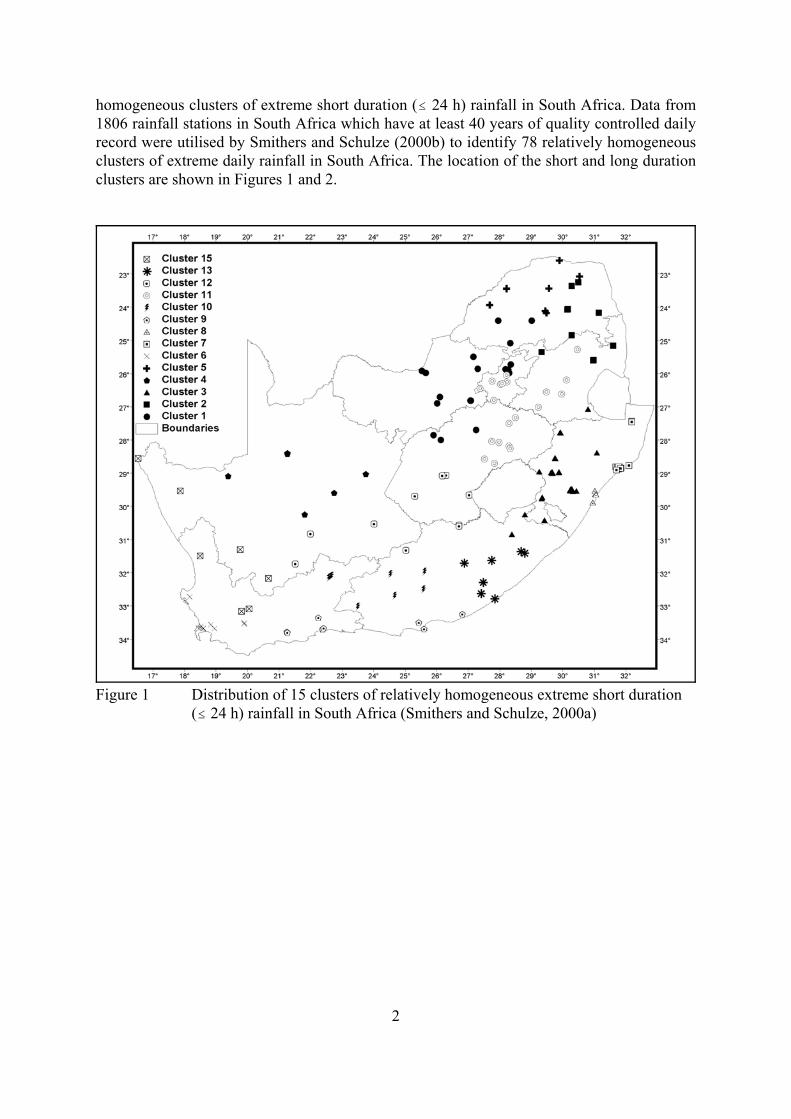
Regional approaches are not new in frequency analysis and many different techniques areavailable. The development of a regional index-flood type approach to frequency analysis basedon L-moments (Hosking and Wallis, 1993; 1997), termed the Regional L-Moment Algorithm(RLMA), has many reported benefits and has been successfully used by Smithers and Schulze(2000a; 2000b) to estimate short (# 24 h) and long (1 to 7 day) duration design rainfall in SouthAfrica.Smithers and Schulze (2000a) utilised digitised rainfall data from 172 recording raingauges inSouth Africa, which each had at least 10 years of record, and identified 15 relatively

2

Figure 1 Distribution of 15 clusters of relatively homogeneous extreme short duration(# 24 h) rainfall in South Africa (Smithers and Schulze, 2000a)

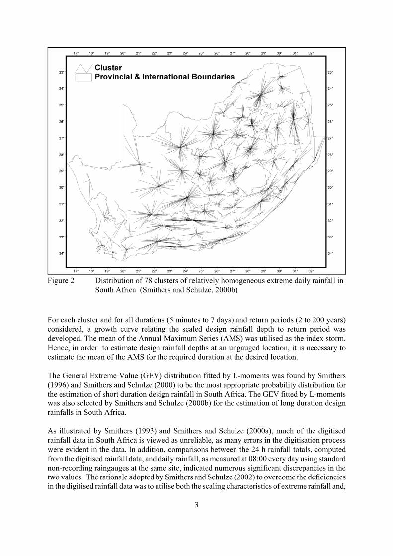
homogeneous clusters of extreme short duration (# 24 h) rainfall in South Africa. Data from1806 rainfall stations in South Africa which have at least 40 years of quality controlled dailyrecord were utilised by Smithers and Schulze (2000b) to identify 78 relatively homogeneousclusters of extreme daily rainfall in South Africa. The location of the short and long durationclusters are shown in Figures 1 and 2.

3

Figure 2 Distribution of 78 clusters of relatively homogeneous extreme daily rainfall inSouth Africa (Smithers and Schulze, 2000b)

For each cluster and for all durations (5 minutes to 7 days) and return periods (2 to 200 years)considered, a growth curve relating the scaled design rainfall depth to return period wasdeveloped. The mean of the Annual Maximum Series (AMS) was utilised as the index storm.Hence, in order to estimate design rainfall depths at an ungauged location, it is necessary toestimate the mean of the AMS for the required duration at the desired location.

The General Extreme Value (GEV) distribution fitted by L-moments was found by Smithers(1996) and Smithers and Schulze (2000) to be the most appropriate probability distribution forthe estimation of short duration design rainfall in South Africa. The GEV fitted by L-momentswas also selected by Smithers and Schulze (2000b) for the estimation of long duration designrainfalls in South Africa.

As illustrated by Smithers (1993) and Smithers and Schulze (2000a), much of the digitisedrainfall data in South Africa is viewed as unreliable, as many errors in the digitisation processwere evident in the data. In addition, comparisons between the 24 h rainfall totals, computedfrom the digitised rainfall data, and daily rainfall, as measured at 08:00 every day using standardnon-recording raingauges at the same site, indicated numerous significant discrepancies in thetwo values. The rationale adopted by Smithers and Schulze (2002) to overcome the deficienciesin the digitised rainfall data was to utilise both the scaling characteristics of extreme rainfall and,

4

as far as possible, the more abundant and reliable daily rainfall data which generally have longerrecord lengths than the digitised rainfall data.

The 24 h AMS are extracted from the digitised rainfall database using a continuously moving24 h “window” to identify the maximum 24 h event. The 1 day AMS contains the maximumevents extracted from the daily rainfall database, which contains 24 h rainfall totals recorded atfixed time intervals.

Smithers and Schulze (2002) developed regionalised regression equations to estimate the meanof the 1 day AMS at any location in South Africa. Thus, using the regionalsied 24 h : 1dayrainfall ratios developed by Smithers and Schulze (2000a), the mean of the 24 h AMS can beestimated at any location in South Africa. The estimation of the mean of the AMS for durations< 24 h has been refined by Smithers and Schulze (2002). For each of the 15 extreme shortduration rainfall clusters and for durations ranging from 5 minutes to 24 h, regression equationsrelating the D h to 24 h mean of the AMS have been developed. Thus, given the estimated meanof the 1 day AMS at the required site, the mean of the AMS for durations #24 h can beestimated. Similarly, regionalised relationships between the D day (2 # D #7) and 1 day AMSwere developed by Smithers and Schulze (2002). Thus, the mean of the AMS for durationsranging from 5 minutes to 7 days can be estimated at any location in South Africa.

Smithers and Schulze (2002) investigated the sampling variability and the effect of unreliabledigitised rainfall data on the development of growth curves. They concluded that the growthcurves were scale invariant and that the growth curve for the 1 day duration, which was deemedto be the most reliable, could thus be applied to durations ranging from 5 minutes to 7 days. Thisregional approach to design rainfall estimation developed by Smithers and Schulze (2002), whichis based on the Regional L-Moment Algorithm (Hosking and Wallis, 1993; Hosking and Wallis,1997), in conjunction with the Scale Invariance of the growth curves (RLMA&SI) has beenshown by Smithers and Schulze (2002) to result in reliable and consistent design values and wasthus utilised in this study to estimate design rainfalls. The RLMA&SI procedure is detailed inthe following chapter.

3 THE RLMA&SI METHODOLOGY FOR DESIGN RAINFALL ESTIMATION

An index storm approach, based on L-moments, has been developed for design rainfallestimation in South Africa (Smithers and Schulze, 2002). Growth curves which relate designrainfall, scaled by the mean of the AMS, to duration are utilised in conjunction with an estimateof the mean of the AMS at the required location to compute the rainfall depth for the specifiedduration and return period. Smithers and Schulze ( 2002) concluded that the growth curves arescale invariant and that the most reliable estimate of the growth curves are those derived fromthe daily rainfall database for the 1 day duration. Thus, the growth curves for the 1 day durationare applied to all durations ranging from 5 minutes to 7 days. Smithers and Schulze (2002)utilised 90% error bounds for the growth curves, which are used in conjunction with the 90%prediction intervals for the mean of the AMS, to estimate 90% error bounds for the designrainfall.

The mean of the 1 day AMS is estimated using regression equations for 7 regions in SouthAfrica, and corrected using a residual error surface. The mean for the 24 h AMS, as would be

5

estimated from continuously recorded rainfall data, is estimated as shown in Equation 2 from the1 day mean of the AMS and the 24 h :1 day ratios developed by Smithers and Schulze (2000a).

...2L L Ratio_ _1 124h day 24h : 1d= ×1

whereL_124h = mean of the 24 h AMS, extracted from digitised rainfall data, L_11day = mean of the 1 day AMS, extracted from daily rainfall data, andRatio24h : 1d = ratio to convert the mean of the 1 day AMS to 24 h AMS.

In order to estimate the means of the AMS for durations of 2 to 7 days, Equation 3 is used:

...3L L 1D D D_ _1 = + ×

φ α 1day

whereL_1D = mean of the AMS for duration = D days, ND = regression constant for duration = D days, and"D = regression coefficient for duration = D days.

Now, the regression constant and coefficient can be estimated from the following equations:

...4α θ τ σD D= + ×

where2 = regression constant ,J = regression coefficient, andF = transformation exponent for duration = D days,

and

...5φ ν κ ρD D= + ×

where< = regression constant,6 = regression coefficient, andD = transformation exponent for duration = D days.

Thus, for a given duration (D), Equations 4 and 5 can be used to estimate the parameters forEquation 3 and hence L_1D (2 #D #7 days) can be estimated using Equation 3.

However, the regressions for different durations may intersect when L_11 day values are usedwhich are outside of the range of values used in the regression analysis. Therefore, it is necessaryto estimate the slope of the relationship between the mean of the AMS (L_1) and duration. Thisis achieved by using L_1 values for durations of 1, 3 and 7 days derived from Equation 3 asshown in Equations 6, 7, 8 and 9.

For durations (D): 1 day < D # 3 day

6

...6SlopeL L

day dayday day

( )

log( _ ) log( _ )log( ) log( )1 3

3 1

3 1− =−

−

1 1

...7[ ][ ]L DL Slope Dday day day_ log( _ ) ) log( ) log( )( )1 1= + × −−10 1 1 3 1

For durations (D): 3 day < D # 7d day

...8SlopeL L

day dayday day

( )

log( _ ) log( _ )log( ) log( )3 7

7 31 13 1− =

−

−

...9[ ][ ]L DL Slope Dday day day_ log( _ ) log( ) log( )( )1 1= + × −−10 3 3 7 3

To estimate the mean of the AMS for durations < 24 h Equation 10 is used:

...10L L XCOEFF CONSTk h i k i k_ ( _ ), ,1 1= × +24

whereL_1k = mean of AMS for duration = k, minutesXCOEFFi,k = regression coefficient for cluster = i and duration = k minutes in

Table ?, andCONSTi,k = regression intercept for cluster = i and duration = k minutes in

Table ?.

Thus L_1k could be estimated for any available duration = k minutes. However, the regressionsfor different durations may intersect when L_124 h values are used which are outside of the rangeof values used in the regression analysis. Thus, it is necessary to estimate the slope of therelationship between L_1 and duration. This is achieved by using L_1 values for durations of 5,15 and 120 minutes derived from Equation 10 and the 24 h value calculated using Equation 2.

For durations (D minutes): 120 < D < 1440

...11SlopeL L

( )

log( _ ) log( _ )log( ) log( )1440 120

1440 120

1440 120− =−−

1 1

...12[ ][ ]L DL Slope Dh_ log( _ ) log( ) log( )( )1 1= − × −−10 24 1440 120 1440

For durations (D minutes): 15 < D < 120

...13SlopeL L

( )

log( _ ) log( _ )log( ) log( )120 15

120 15

120 15− =−−

1 1

...14[ ][ ]L DL Slope D_ log( _ ) log( ) log( )( )1 = − × −−10 120 120 15 1201

For durations (D minutes): 5 < D < 15

7

...15SlopeL L

( )

log( _ ) log( _ )log( ) log( )15 5

15 5

15 5− =−−

1 1

...16[ ][ ]L DL Slope D_ log( _ ) log( ) log( )( )1 = − × −−10 1 1515 15 5

Design rainfall depths are calculated using Equation 17.

...17DRE GC L_1i, j i, j i= ×where

DREi,j = design rainfall estimate for duration = i and return period = j,GCi,,j = growth curve for duration = i and return period = j, andL_1i = mean of AMS for duration = i estimated using the above procedures.

However, as shown by Smithers and Schulze (2002), the best estimate of the growth curve forall durations are the values derived from the daily rainfall database for the 1 day duration. HenceEquation 17 may be re-written as:

...18DRE GC L_1i, j 1 day, j= × i

The 90 % prediction interval for DREi,j is estimated by:

...19U U U

L L L i

90 90 90

90 90 90

DRE GC L_1

DRE GC L_1i, j i, day i

i, j i, day

= ×

= ×1

1

whereU90DREi,j = upper 90% error bound of design rainfall estimated for duration = i and

return period = j,U90GCi,j = upper 90% error bound of the growth curve for duration = i and return

period = j,U90L_1i = upper 90% error bound of the estimated mean of annual maximum series

for duration=i,L90DREi,j = lower 90% error bound of design rainfall estimated for duration = i and

return period = j,L90GCi,j = lower 90% error bound of the growth curve for duration = i and return

period = j, andL90L_1i = lower 90% error bound of the estimated mean of annual maximum series

for duration=i.

The prediction interval for the mean of the AMS is symmetrical about the estimated value andhence may be represented as

8

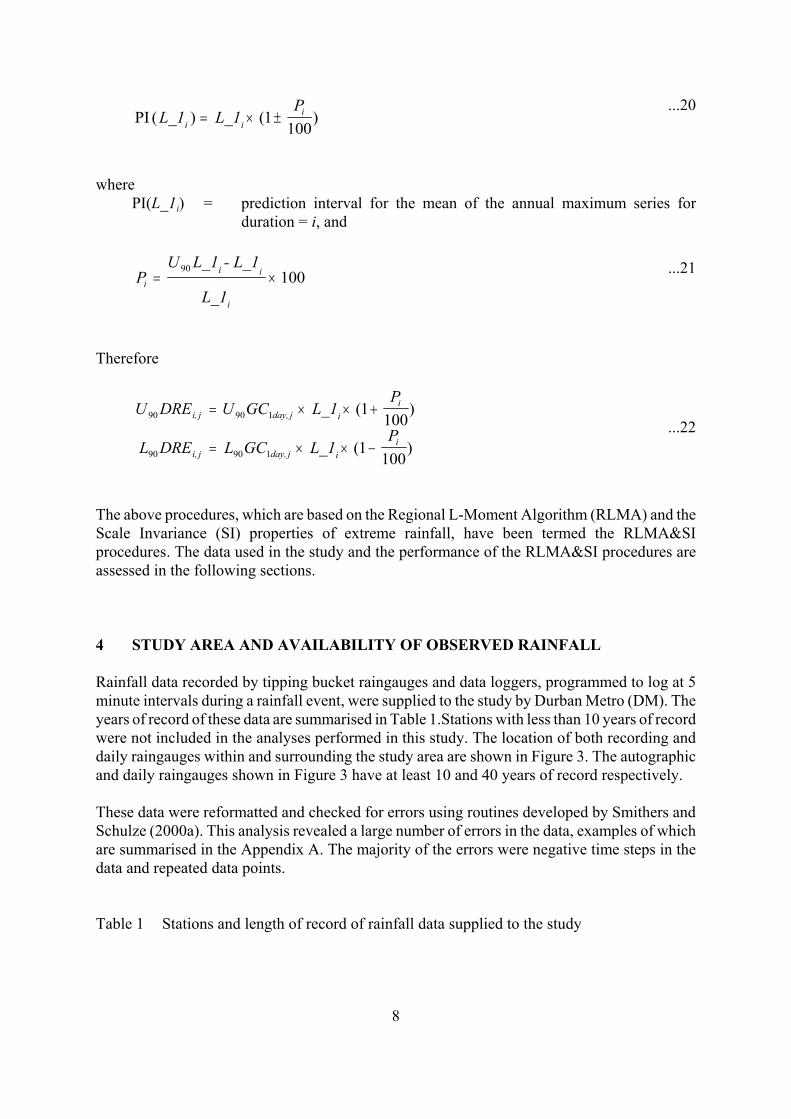
...20PI 1( ) ( )L_1 L_1

Pi i

i= × ±100

wherePI(L_1i) = prediction interval for the mean of the annual maximum series for

duration = i, and

...21PU L_1 - L_1

L_1

i i

i

i = ×90

100

Therefore

...22U U

P

L LP

i

i

90 90

90 90

1100

1100

DRE GC L_1

DRE GC L_1

i, j day, j i

i, j day, j i

= × × +

= × × −

1

1

( )

( )

The above procedures, which are based on the Regional L-Moment Algorithm (RLMA) and theScale Invariance (SI) properties of extreme rainfall, have been termed the RLMA&SIprocedures. The data used in the study and the performance of the RLMA&SI procedures areassessed in the following sections.

4 STUDY AREA AND AVAILABILITY OF OBSERVED RAINFALL

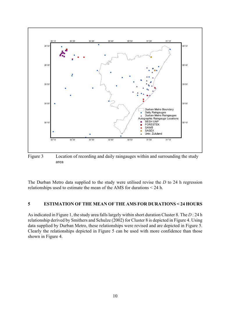
Rainfall data recorded by tipping bucket raingauges and data loggers, programmed to log at 5minute intervals during a rainfall event, were supplied to the study by Durban Metro (DM). Theyears of record of these data are summarised in Table 1.Stations with less than 10 years of recordwere not included in the analyses performed in this study. The location of both recording anddaily raingauges within and surrounding the study area are shown in Figure 3. The autographicand daily raingauges shown in Figure 3 have at least 10 and 40 years of record respectively.

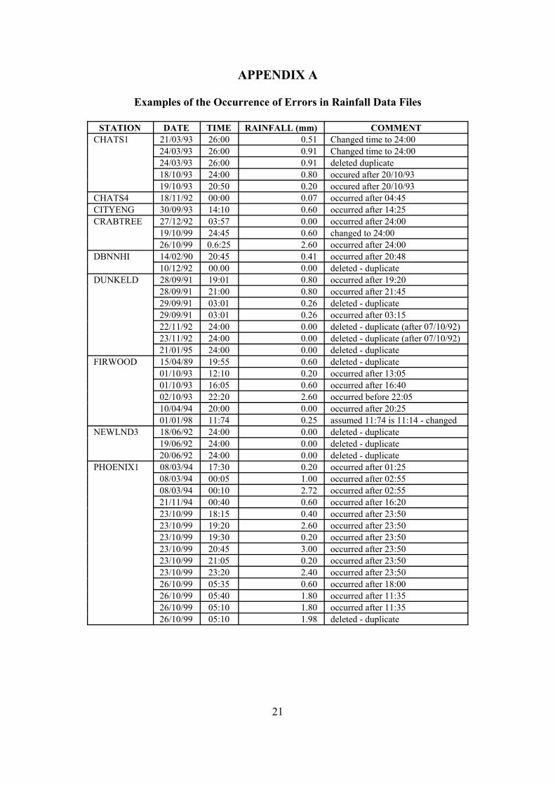
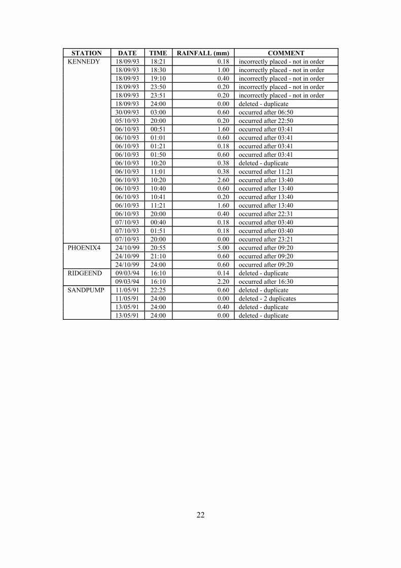
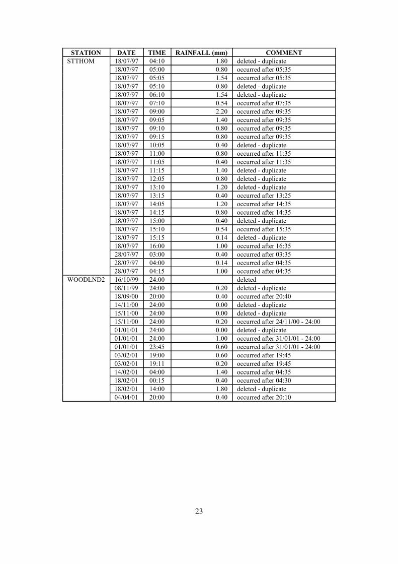
These data were reformatted and checked for errors using routines developed by Smithers andSchulze (2000a). This analysis revealed a large number of errors in the data, examples of whichare summarised in the Appendix A. The majority of the errors were negative time steps in thedata and repeated data points.

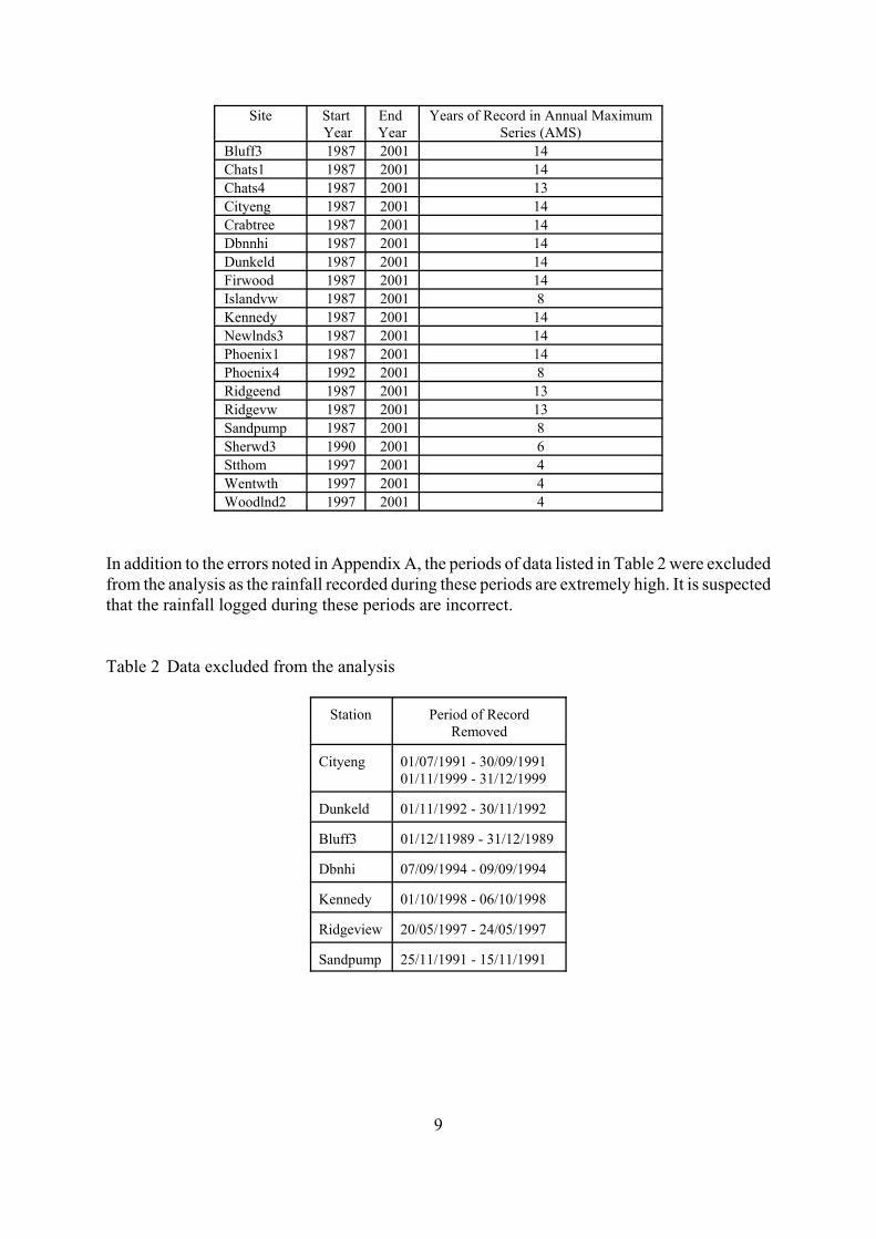
Table 1 Stations and length of record of rainfall data supplied to the study

9

Site Start Year

End Year

Years of Record in Annual MaximumSeries (AMS)

Bluff3 1987 2001 14Chats1 1987 2001 14Chats4 1987 2001 13Cityeng 1987 2001 14Crabtree 1987 2001 14Dbnnhi 1987 2001 14Dunkeld 1987 2001 14Firwood 1987 2001 14Islandvw 1987 2001 8Kennedy 1987 2001 14Newlnds3 1987 2001 14Phoenix1 1987 2001 14Phoenix4 1992 2001 8Ridgeend 1987 2001 13Ridgevw 1987 2001 13Sandpump 1987 2001 8Sherwd3 1990 2001 6Stthom 1997 2001 4Wentwth 1997 2001 4Woodlnd2 1997 2001 4

In addition to the errors noted in Appendix A, the periods of data listed in Table 2 were excludedfrom the analysis as the rainfall recorded during these periods are extremely high. It is suspectedthat the rainfall logged during these periods are incorrect.

Table 2 Data excluded from the analysis

Station Period of RecordRemoved

Cityeng 01/07/1991 - 30/09/199101/11/1999 - 31/12/1999

Dunkeld 01/11/1992 - 30/11/1992

Bluff3 01/12/11989 - 31/12/1989

Dbnhi 07/09/1994 - 09/09/1994

Kennedy 01/10/1998 - 06/10/1998

Ridgeview 20/05/1997 - 24/05/1997

Sandpump 25/11/1991 - 15/11/1991

10

Figure 3 Location of recording and daily raingauges within and surrounding the studyarea

The Durban Metro data supplied to the study were utilised revise the D to 24 h regressionrelationships used to estimate the mean of the AMS for durations < 24 h.

5 ESTIMATION OF THE MEAN OF THE AMS FOR DURATIONS < 24 HOURS

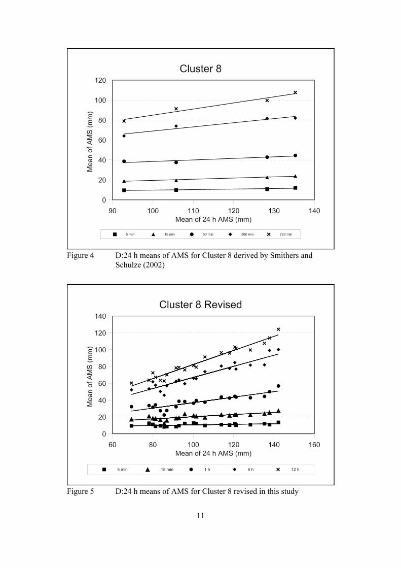
As indicated in Figure 1, the study area falls largely within short duration Cluster 8. The D : 24 hrelationship derived by Smithers and Schulze (2002) for Cluster 8 is depicted in Figure 4. Usingdata supplied by Durban Metro, these relationships were revised and are depicted in Figure 5.Clearly the relationships depicted in Figure 5 can be used with more confidence than thoseshown in Figure 4.

11

Figure 4 D:24 h means of AMS for Cluster 8 derived by Smithers andSchulze (2002)

Figure 5 D:24 h means of AMS for Cluster 8 revised in this study

12

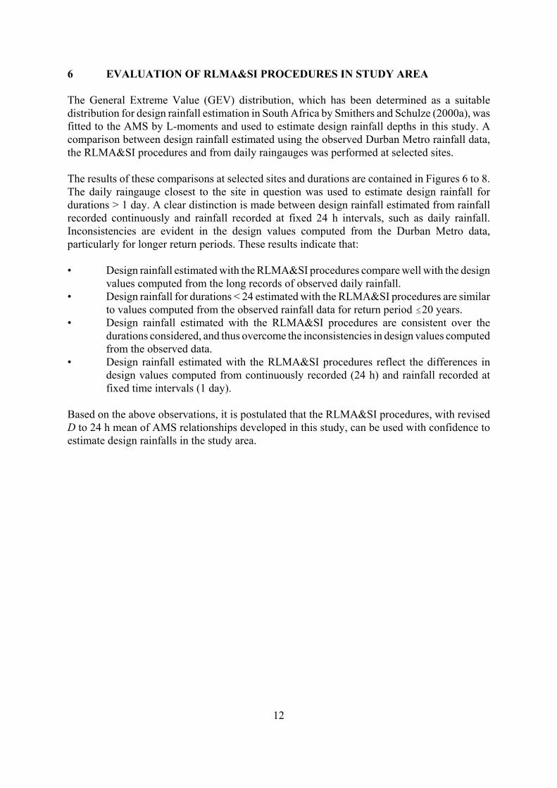
6 EVALUATION OF RLMA&SI PROCEDURES IN STUDY AREA

The General Extreme Value (GEV) distribution, which has been determined as a suitabledistribution for design rainfall estimation in South Africa by Smithers and Schulze (2000a), wasfitted to the AMS by L-moments and used to estimate design rainfall depths in this study. Acomparison between design rainfall estimated using the observed Durban Metro rainfall data,the RLMA&SI procedures and from daily raingauges was performed at selected sites.

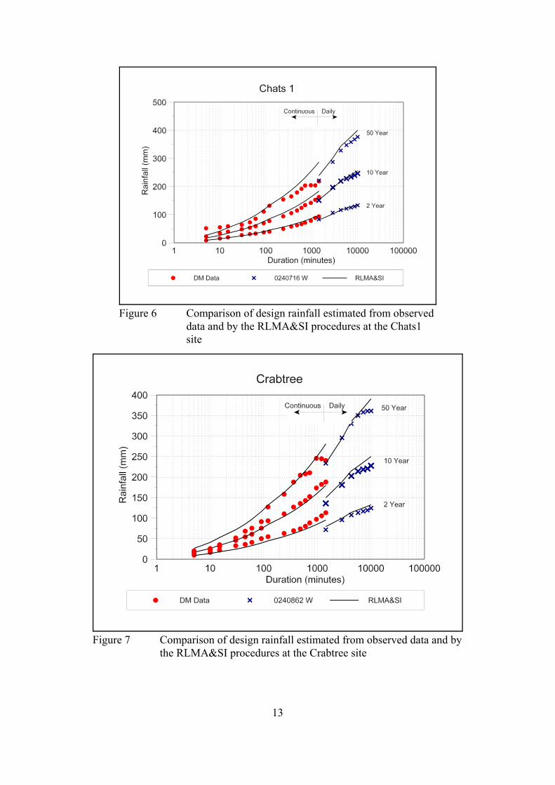
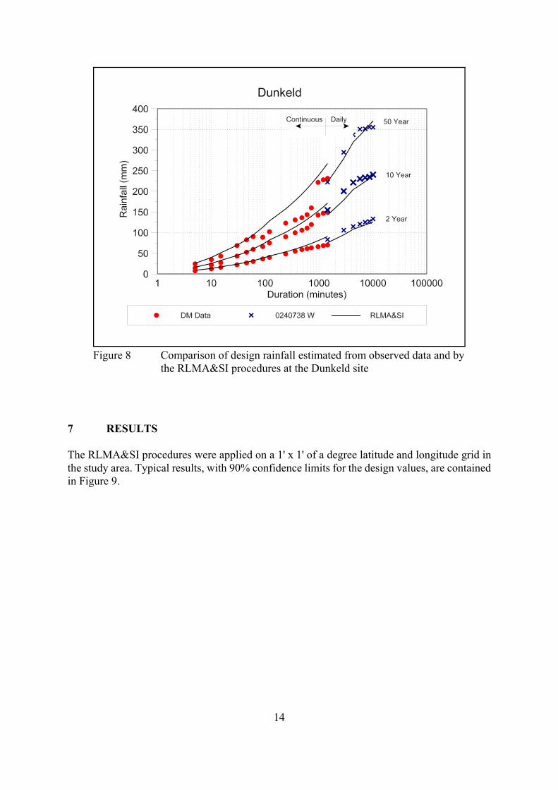
The results of these comparisons at selected sites and durations are contained in Figures 6 to 8.The daily raingauge closest to the site in question was used to estimate design rainfall fordurations > 1 day. A clear distinction is made between design rainfall estimated from rainfallrecorded continuously and rainfall recorded at fixed 24 h intervals, such as daily rainfall.Inconsistencies are evident in the design values computed from the Durban Metro data,particularly for longer return periods. These results indicate that:

• Design rainfall estimated with the RLMA&SI procedures compare well with the designvalues computed from the long records of observed daily rainfall.

• Design rainfall for durations < 24 estimated with the RLMA&SI procedures are similarto values computed from the observed rainfall data for return period #20 years.

• Design rainfall estimated with the RLMA&SI procedures are consistent over thedurations considered, and thus overcome the inconsistencies in design values computedfrom the observed data.

• Design rainfall estimated with the RLMA&SI procedures reflect the differences indesign values computed from continuously recorded (24 h) and rainfall recorded atfixed time intervals (1 day).

Based on the above observations, it is postulated that the RLMA&SI procedures, with revisedD to 24 h mean of AMS relationships developed in this study, can be used with confidence toestimate design rainfalls in the study area.

13

Figure 6 Comparison of design rainfall estimated from observeddata and by the RLMA&SI procedures at the Chats1site

Figure 7 Comparison of design rainfall estimated from observed data and bythe RLMA&SI procedures at the Crabtree site

14

Figure 8 Comparison of design rainfall estimated from observed data and bythe RLMA&SI procedures at the Dunkeld site

7 RESULTS

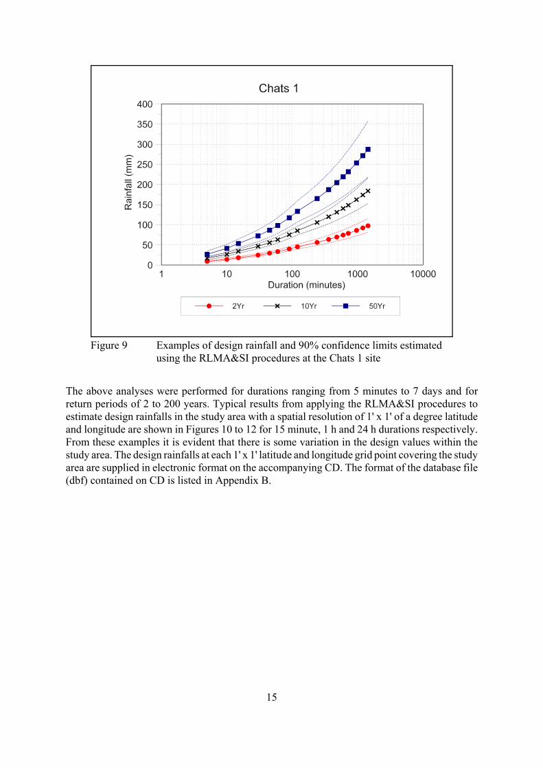
The RLMA&SI procedures were applied on a 1' x 1' of a degree latitude and longitude grid inthe study area. Typical results, with 90% confidence limits for the design values, are containedin Figure 9.

15

Figure 9 Examples of design rainfall and 90% confidence limits estimatedusing the RLMA&SI procedures at the Chats 1 site

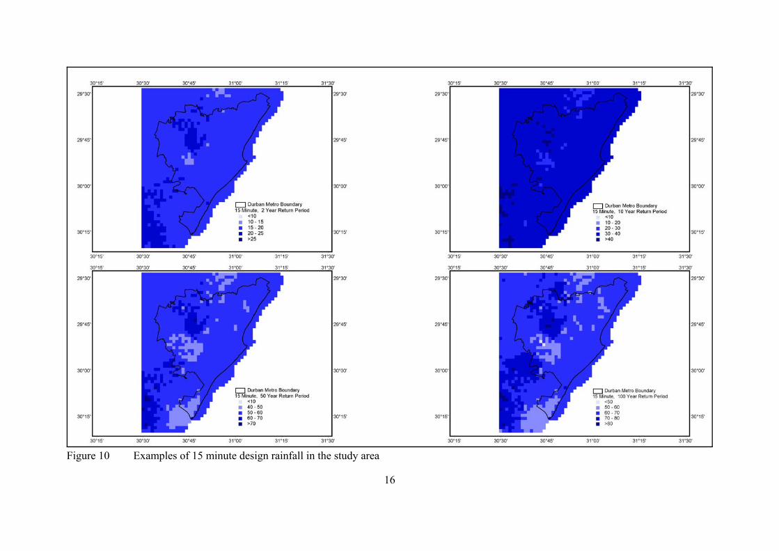
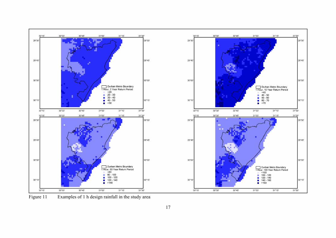
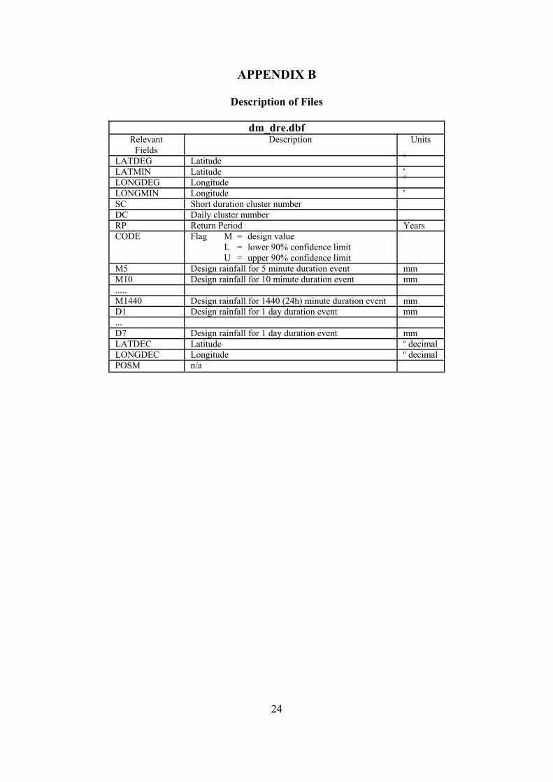
The above analyses were performed for durations ranging from 5 minutes to 7 days and forreturn periods of 2 to 200 years. Typical results from applying the RLMA&SI procedures toestimate design rainfalls in the study area with a spatial resolution of 1' x 1' of a degree latitudeand longitude are shown in Figures 10 to 12 for 15 minute, 1 h and 24 h durations respectively.From these examples it is evident that there is some variation in the design values within thestudy area. The design rainfalls at each 1' x 1' latitude and longitude grid point covering the studyarea are supplied in electronic format on the accompanying CD. The format of the database file(dbf) contained on CD is listed in Appendix B.

16

Figure 10 Examples of 15 minute design rainfall in the study area

17

Figure 11 Examples of 1 h design rainfall in the study area

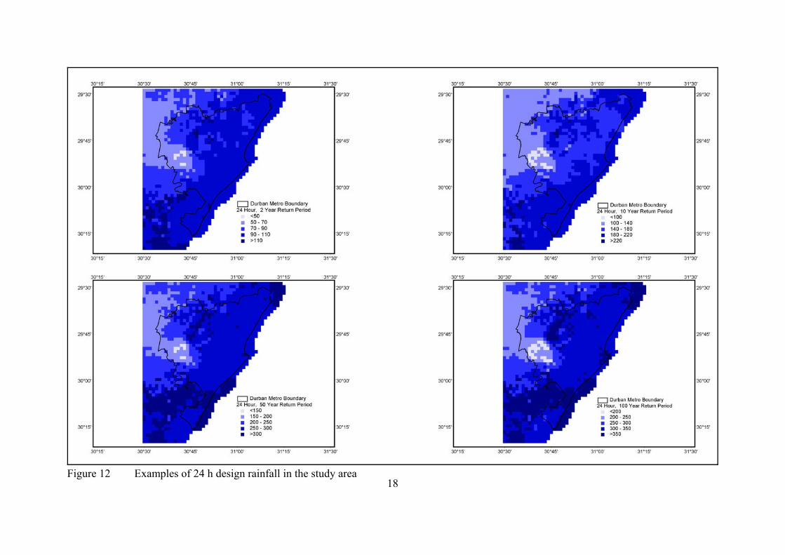
18Figure 12 Examples of 24 h design rainfall in the study area

19

8 DISCUSSION AND CONCLUSIONS

The regional approach as developed by Smithers and Schulze (2000a), and further refined andtermed the RLMA&SI procedures by Smithers and Schulze (2002), has been utilised andrefined to estimate short duration design rainfalls for the study area which encompasses theeThekwini Metropolitan Municipality's area of jurisdiction. This approach differs from thesingle site approach to design rainfall estimation used by, for example, Midgley and Pitman(1978), Alexander (1978; 1990), Adamson (1981), Schulze (1984) and Weddepohl (1988), andimproves the reliability of the design values.

The RLMA&SI procedures developed by Smithers and Schulze (2002) to estimate designrainfalls in South Africa have been applied in the study area on a 1' x 1' latitude and longitudegrid. These estimates have been compared to values estimated directly from the observed rainfalldata. In this study it has been shown that the RLMA&SI procedures generally result in consistentand reliable estimates of design rainfall, which are similar to design values estimated directlyfrom observed rainfall data. Design rainfall estimated using the RLMA&SI procedures are notaffected by at-site anomalies in the data. Daily rainfall data, which have longer records than thecontinuously recorded rainfall, are utilised in the analysis. In addition, the regional approach isfar more detailed and is based on an analysis of longer periods of records from more stations thanany other previous study on rainfall frequency analysis in South Africa. With the refinement ofthe relationship between the D h and 24 h mean of the AMS using data from the study area, itis postulated that the estimated design rainfalls may be used with confidence within the studyarea.

A listing and description of files containing the results generated in this study are contained inAppendix B.

9 REFERENCES

Adamson, P.T., 1981. Southern African storm rainfall. Technical Report No. TR 102.Department of Water Affairs, Pretoria, RSA.

Alexander, W.J.R., 1978. Depth-area-duration-frequency properties of storm precipitation inSouth Africa. Technical Report No. TR 83. Department of Water Affairs, Pretoria,RSA.

Alexander, W.J.R., 1990. Flood Hydrology for Southern Africa. SANCOLD, Pretoria, RSA.Alexander, W.J.R., 2001. Flood Risk Reduction Measures. University of Pretoria, Pretoria, RSA.Cunnane, C., 1989. Statistical distributions for flood frequency analysis. WMO Report No. 718.

World Meteorological Organization, Geneva, Switzerland. Dent, M.C., Lynch, S.D. and Schulze, R.E., 1987. Mapping mean annual and other rainfall

statistics over southern Africa. Report 109/1/89. Water Research Commission, Pretoria,RSA. 198 plus Appendices pp.

Gabriele, S. and Arnell, N., 1991. A hierarchical approach to regional flood frequency analysis.Water Resources Research, 27(6): 1281-1289.

Hosking, J.R.M. and Wallis, J.R., 1987. An index flood procedure for regional rainfall frequencyanalysis. EOS, Transactions, American Geophysical Union, 68: 312.

20

Hosking, J.R.M. and Wallis, J.R., 1993. Some statistics useful in a regional frequency analysis.Water Resources Research, 29(2): 271-281.

Hosking, J.R.M. and Wallis, J.R., 1997. Regional Frequency Analysis: An Approach Based onL-Moments. Cambridge University Press, Cambridge, UK. 224 pp.

Lettenmaier, D.P., 1985. Regionalisation in flood frequency analysis - Is it the answer ? US-China Bilateral Symposium on the Analysis of Extraordinary Flood Events. Nanjing,China.

Lettenmaier, D.P. and Potter, K.W., 1985. Testing flood frequency estimation methods using aregional flood generation model. Water Resources Research, 21: 1903-1914.

Midgley, D.C. and Pitman, W.V., 1978. A depth-duration-frequency diagram for point rainfallin Southern Africa. HRU Report 2/78. University of Witwatersrand, Johannesburg,RSA. 57 pp.

Nandakumar, N., 1995. Estimation of extreme rainfalls for Victoria - Application of the Forgemethod. Working Document 95/7. Cooperative Research Centre for CatchmentHydrology, Monash University, Clayton, Victoria, Australia.

Op Ten Noort, T.H., 1983. Flood peak estimation in South Africa. The Civil Engineer in SouthAfrica, October: 557-563.

Pilon, P.J. and Adamowski, K., 1992. The value of regional information to flood frequencyanalysis using the method of L-moments. Canadian Journal of Civil Engineering, 19(1):137-147.

Potter, K.W., 1987. Research on flood frequency analysis: 1983-1986. Review of Geophysics,25(2): 113-118.

Schaefer, M.G., 1990. Regional analyses of precipitation annual maxima in Washington State.Water Resources Research, 26(1): 119-131.

Schmidt, E.J. and Schulze, R.E., 1987. SCS-based design runoff. ACRU Report No. 24.Department of Agricultural Engineering, University of Natal, Pietermaritzburg, RSA.164 pp.

Schulze, R.E., 1984. Depth-duration-frequency studies in Natal based on digitised data. In: H.Maaren (Editor). South African National Hydrology Symposium. Department ofEnvironment Affairs, Technical Report TR119. Pretoria, RSA. 214-235.

Smithers, J.C., 1993. The effect on design rainfall estimates of errors in the digitised rainfalldatabase. In: S.A. Lorentz, S.W. Kienzle and M.C. Dent (Editors). Proceedings of theSixth South African National Hydrological Symposium. Department of AgriculturalEngineering, University of Natal. Pietermaritzburg, RSA. 95-102.

Smithers, J.C., 1996. Short-duration rainfall frequency model selection in Southern Africa.Water SA, 22(3): 211-217.

Smithers, J.C. and Schulze, R.E., 2000a. Development and evaluation of techniques forestimating short duration design rainfall in South Africa. WRC Report No. 681/1/00.Water Research Commission, Pretoria, RSA. 356 pp.

Smithers, J.C. and Schulze, R.E., 2000b. Long duration design rainfall estimates for SouthAfrica. WRC Report No. 811/1/00. Water Research Commission, Pretoria, RSA. 69 pp.

Smithers, J.C. and Schulze, R.E., 2002. Design rainfall and flood estimation in South Africa.WRC Project No. K5/1060. Draft final report (Project K5/1060) to Water ResearchCommission, Pretoria, RSA. 155 pp.

Stedinger, J.R., Vogel, R.M. and Foufoula-Georgiou, E., 1993. Frequency analysis of extremeevents. Handbook of Hydrology. McGraw-Hill, New York, USA.

Weddepohl, J.P., 1988. Design rainfall distributions for Southern Africa. Unpublished M.Sc.Dissertation, Department of Agricultural Engineering, University of Natal,Pietermaritzburg, RSA.

21

APPENDIX A

Examples of the Occurrence of Errors in Rainfall Data Files

STATION DATE TIME RAINFALL (mm) COMMENTCHATS1 21/03/93 26:00 0.51 Changed time to 24:00

24/03/93 26:00 0.91 Changed time to 24:0024/03/93 26:00 0.91 deleted duplicate18/10/93 24:00 0.80 occured after 20/10/9319/10/93 20:50 0.20 occured after 20/10/93

CHATS4 18/11/92 00:00 0.07 occurred after 04:45CITYENG 30/09/93 14:10 0.60 occurred after 14:25CRABTREE 27/12/92 03:57 0.00 occurred after 24:00

19/10/99 24:45 0.60 changed to 24:0026/10/99 0.6:25 2.60 occurred after 24:00

DBNNHI 14/02/90 20:45 0.41 occurred after 20:4810/12/92 00.00 0.00 deleted - duplicate

DUNKELD 28/09/91 19:01 0.80 occurred after 19:2028/09/91 21:00 0.80 occurred after 21:4529/09/91 03:01 0.26 deleted - duplicate29/09/91 03:01 0.26 occurred after 03:1522/11/92 24:00 0.00 deleted - duplicate (after 07/10/92)23/11/92 24:00 0.00 deleted - duplicate (after 07/10/92)21/01/95 24:00 0.00 deleted - duplicate

FIRWOOD 15/04/89 19:55 0.60 deleted - duplicate01/10/93 12:10 0.20 occurred after 13:0501/10/93 16:05 0.60 occurred after 16:4002/10/93 22:20 2.60 occurred before 22:0510/04/94 20:00 0.00 occurred after 20:2501/01/98 11:74 0.25 assumed 11:74 is 11:14 - changed

NEWLND3 18/06/92 24:00 0.00 deleted - duplicate19/06/92 24:00 0.00 deleted - duplicate20/06/92 24:00 0.00 deleted - duplicate

PHOENIX1 08/03/94 17:30 0.20 occurred after 01:2508/03/94 00:05 1.00 occurred after 02:5508/03/94 00:10 2.72 occurred after 02:5521/11/94 00:40 0.60 occurred after 16:2023/10/99 18:15 0.40 occurred after 23:5023/10/99 19:20 2.60 occurred after 23:5023/10/99 19:30 0.20 occurred after 23:5023/10/99 20:45 3.00 occurred after 23:5023/10/99 21:05 0.20 occurred after 23:5023/10/99 23:20 2.40 occurred after 23:5026/10/99 05:35 0.60 occurred after 18:0026/10/99 05:40 1.80 occurred after 11:3526/10/99 05:10 1.80 occurred after 11:3526/10/99 05:10 1.98 deleted - duplicate

STATION DATE TIME RAINFALL (mm) COMMENT

22

KENNEDY 18/09/93 18:21 0.18 incorrectly placed - not in order18/09/93 18:30 1.00 incorrectly placed - not in order18/09/93 19:10 0.40 incorrectly placed - not in order18/09/93 23:50 0.20 incorrectly placed - not in order18/09/93 23:51 0.20 incorrectly placed - not in order18/09/93 24:00 0.00 deleted - duplicate30/09/93 03:00 0.60 occurred after 06:5005/10/93 20:00 0.20 occurred after 22:5006/10/93 00:51 1.60 occurred after 03:4106/10/93 01:01 0.60 occurred after 03:4106/10/93 01:21 0.18 occurred after 03:4106/10/93 01:50 0.60 occurred after 03:4106/10/93 10:20 0.38 deleted - duplicate06/10/93 11:01 0.38 occurred after 11:2106/10/93 10:20 2.60 occurred after 13:4006/10/93 10:40 0.60 occurred after 13:4006/10/93 10:41 0.20 occurred after 13:4006/10/93 11:21 1.60 occurred after 13:4006/10/93 20:00 0.40 occurred after 22:3107/10/93 00:40 0.18 occurred after 03:4007/10/93 01:51 0.18 occurred after 03:4007/10/93 20:00 0.00 occurred after 23:21

PHOENIX4 24/10/99 20:55 5.00 occurred after 09:2024/10/99 21:10 0.60 occurred after 09:2024/10/99 24:00 0.60 occurred after 09:20

RIDGEEND 09/03/94 16:10 0.14 deleted - duplicate09/03/94 16:10 2.20 occurred after 16:30

SANDPUMP 11/05/91 22:25 0.60 deleted - duplicate11/05/91 24:00 0.00 deleted - 2 duplicates13/05/91 24:00 0.40 deleted - duplicate13/05/91 24:00 0.00 deleted - duplicate

STATION DATE TIME RAINFALL (mm) COMMENT

23

STTHOM 18/07/97 04:10 1.80 deleted - duplicate18/07/97 05:00 0.80 occurred after 05:3518/07/97 05:05 1.54 occurred after 05:3518/07/97 05:10 0.80 deleted - duplicate18/07/97 06:10 1.54 deleted - duplicate18/07/97 07:10 0.54 occurred after 07:3518/07/97 09:00 2.20 occurred after 09:3518/07/97 09:05 1.40 occurred after 09:3518/07/97 09:10 0.80 occurred after 09:3518/07/97 09:15 0.80 occurred after 09:3518/07/97 10:05 0.40 deleted - duplicate18/07/97 11:00 0.80 occurred after 11:3518/07/97 11:05 0.40 occurred after 11:3518/07/97 11:15 1.40 deleted - duplicate18/07/97 12:05 0.80 deleted - duplicate18/07/97 13:10 1.20 deleted - duplicate18/07/97 13:15 0.40 occurred after 13:2518/07/97 14:05 1.20 occurred after 14:3518/07/97 14:15 0.80 occurred after 14:3518/07/97 15:00 0.40 deleted - duplicate18/07/97 15:10 0.54 occurred after 15:3518/07/97 15:15 0.14 deleted - duplicate18/07/97 16:00 1.00 occurred after 16:3528/07/97 03:00 0.40 occurred after 03:3528/07/97 04:00 0.14 occurred after 04:3528/07/97 04:15 1.00 occurred after 04:35

WOODLND2 16/10/99 24:00 deleted08/11/99 24:00 0.20 deleted - duplicate18/09/00 20:00 0.40 occurred after 20:4014/11/00 24:00 0.00 deleted - duplicate15/11/00 24:00 0.00 deleted - duplicate15/11/00 24:00 0.20 occurred after 24/11/00 - 24:0001/01/01 24:00 0.00 deleted - duplicate01/01/01 24:00 1.00 occurred after 31/01/01 - 24:0001/01/01 23:45 0.60 occurred after 31/01/01 - 24:0003/02/01 19:00 0.60 occurred after 19:4503/02/01 19:11 0.20 occurred after 19:4514/02/01 04:00 1.40 occurred after 04:3518/02/01 00:15 0.40 occurred after 04:3018/02/01 14:00 1.80 deleted - duplicate04/04/01 20:00 0.40 occurred after 20:10

24

APPENDIX B

Description of Files

dm_dre.dbfRelevant

FieldsDescription Units

LATDEG Latitudeo

LATMIN Latitude 'LONGDEG Longitude

o

LONGMIN Longitude 'SC Short duration cluster numberDC Daily cluster numberRP Return Period YearsCODE Flag M = design value

L = lower 90% confidence limitU = upper 90% confidence limit

M5 Design rainfall for 5 minute duration event mmM10 Design rainfall for 10 minute duration event mm.....M1440 Design rainfall for 1440 (24h) minute duration event mmD1 Design rainfall for 1 day duration event mm...D7 Design rainfall for 1 day duration event mmLATDEC Latitude o decimalLONGDEC Longitude o decimalPOSM n/a