THE EUROPEAN SYNCHROTRON RADIATION FACILITY

HYDROSTATIC LEVELING SYSTEM –TWELVE YEARS

EXPERIENCE WITH A LARGE SCALE HYDROSTATIC LEVELING

SYSTEM

D. Martin

With special acknowledgements to G. Gatta, B. Perret and E. Claret

E.S.R.F., Grenoble, France

1. INTRODUCTION

This paper will discuss the European Synchrotron Radiation Facility (ESRF) Hydrostatic

Leveling Systems (HLS) composed over 500 sensors. Note that in this discussion an HLS

instrument will generally be referred to as a captor or sensor. This generic term refers to the

capacitive sensor, the vessel and the temperature sensor ensemble. Refer to figure 1 for a

schematic of the ESRF HLS instrument as well as its situation in the Storage Ring. We will

dwell principally on the performance of the two main systems, the so-called first generation

and second generation HLS, The main effort will be made to discuss how to qualify a large

scale HLS.

The ESRF HLS systems as any HLS are based on a water (or liquid) equipotential surface

common to all measuring points. The ESRF instruments are composed of three parts. The

captor vessel which holds the liquid, a capacitive sensor measuring the capacitance

(proportional to distance) between its electrode and the water surface and a temperature

sensor used to correct the dilation of water as a function of temperature between the different

vessels in the system

1.1 FIRST GENERATION STORAGE RING HLS

Note that in this discussion First Generation and SR HLS will be used interchangeably.

This original system was conceived and installed to minimize the number of leveling surveys

by providing a reliable real time height difference measure over a long (several month) time

period, to control the vertical movements made by the Steinsvik Maskinindustrie jacks during

a machine realignment, and finally to follow machine and ground motion events in real time.

As will be shown, these objectives have met with a varying degree of success

The first generation HLS is composed of 288 sensors three each installed on the 96

quadrupole girders in the Storage Ring (SR). The system has a precision of ~1 to 3 µm over

short time spans (less than 24 to 48 hours). It is robust and relatively trouble free. The captors

have been gathering data 24 hours per day over the last 12 years with only a handful of

breakdowns.

1.2 SECOND GENERATION STORAGE RING HLS

This system was conceived and installed to follow the evolution of the beam line front

ends and to provide a real time level reference in the beam line optical hutches. For a number

of reasons, these objectives were abandoned and ultimately the system was installed on the

SR tunnel roof to provide a real time monitoring of site evolution in the vertical direction. It

was also installed to provide large scale HLS qualification test system.

The second generation HLS is presently installed on the SR tunnel roof above the centers

of the quadrupole girders. All sensors are installed on the interior wall with the exception of

the injection zone area where they are installed on the exterior wall. Note that in this

discussion Second Generation and Roof HLS will be used interchangeably. This installation

is shown in figure 2.

2. HLS QUALIFICATION INTERNAL AND EXTERNAL COHERENCE

An HLS system’s coherence can be qualified in two ways. The first, internal coherence

refers how the system reacts with respect to known events such as a variation in the fluid

level. Three examples are filling/purging of the system, electrical cut test (for SR) and most

importantly the long-term stability followed in a controlled environment such as on a

metrological marble. External coherence refers how well the HLS results agree with an

independent control that has a well-established incertitude. Three examples are once again

long term stability on a marble, machine alignment with the motorized jacks and control with

the SR beam, and level and tilt surveys.

Fig. 1 Schematic of the ESRF HLS and its situation in the storage ring

equipotential

surface

capacitive sensor

temperature sensor

= Cε A

d

water tube

air

valve/tap

HLS sensors

Steinsvik Maskinindustrie jacks

equipotential

surface

capacitive sensor

temperature sensor

= Cε A

d

water tube

air

valve/tap

HLS sensors

Steinsvik Maskinindustrie jacks

Fig. 2 Installation of the so-called roof HLS second generation HLS

2.1 HLS QUALIFICATION INTERNAL COHERENCE The variation of the fluid level by either filling and/or purging has long been used at the ESRF to qualify the system coherence of an HLS. It provides two key controls: first that there is fluid communication between all of the vessels ensuring proper operation and a true equipotential reference surface; and secondly it verifies the sensor linearity over its full measurement range. Figure 3 shows the purging of the system over the period December 23 to 26, 1993. In the upper left corner we see the mean level of the system over this period. The upper right graph shows how the full system evolved over the period. The bottom graph shows the stability of the system with a standard deviation of 1 µm over the four hours prior to the operation.

Fig. 3 Purging of the storage ring HLS 23 to 26 December 1993

Fig. 3 Purging of the Storage Ring HLS 23 to 26 December 1993

Fig. 4 Purging of the Storage Ring HLS 23 to 26 December 1993 2 to 6 hours after the

purging start.

The subsequent figures 4, 5 and 6 show the evolution of the system immediately after, and 12 and 24 hours after the purging start. As one can see, although the system is seriously perturbed, it forms a smooth wave. A Fourier series (for example) can be used to model this smooth wave. Theoretically, if the system is functioning correctly, residuals from the smooth curve should be zero. However, in reality, small movements will occur and residuals with respect to the smooth curve represent a combination of these movements and departures from linearity over the measurement range for the system. For this reason it is extremely important to conduct this test during a calm period. These residuals are shown in the graphs at the bottom of figures 3 through 6. A resume of the situation for this test is given in table 1. The system is operating correctly in this instance. For comparison, figure 7 shows the system performance over a calm five-day period in September 2000. This figure gives an indication of the natural temporal change in the system under calm conditions. On the left of this figure is the development around the ring with respect to the origin for each hour over the five-day period. Of the right is the standard deviation of all of the captors with respect to their initial position as a function of time. There is degradation in the standard deviation of 2.5 µm in 48 hours. Generally, sensor linearity should only be an issue if there are large variations over time. At the ESRF this is not the case. Typical real peak-to-peak movements are in the order of ±300 µm per six months. Furthermore the water level doesn’t vary significantly over time. When there is a blockage in the system, a discontinuity in the wave is formed.

Time after purge start

"Wave" peak to peak (µm)

standard deviation of residuals with respect to the “Wave” (µm)

-2 ± 4 1

2 ± 1000 3

12 ± 250 6

24 ± 80 9

48 ± 40 13

Fig. 5 Purging of the Storage Ring HLS 23 to 26 December 1993 10 to 14 hours after the

purging start.

Figure 6 Purging of the Storage Ring HLS 23 to 26 December 1993 22 to 26 hours after the purging start.

-40

-20

0

20

40

dH o

ver 1

20 H

our P

erio

d 7

to

11 S

epte

mbe

r (µm

)

02468

1012

0 24 48 72 96 120Stan

dard

Dev

iatio

n of

HLS

(µ

m)

Fig. 7 Perturbations to the SR HLS system over a calm five-day period in September 2000.

The most important internal coherence test is the captor long-term stability. Captor long-term stability refers to coherence between real height difference and those reported by the HLS. This test should be performed on every HLS captor over a sufficiently long time period so as to demonstrate its temporal stability. At the ESRF this is conducted in a temperature controlled laboratory on a metrological marble. The marble is massive and no flexion is to be expected. All HLS are fixed to the marble and can only move as an ensemble in a plane. Theoretically after the planar movements have been modeled and removed from the captor readings we should see no movement between the different sensors. Figure 8 shows the results of tests made on the first generation SR HLS over the three-month period April to July 1997. As can be seen, the overall standard deviation is 16.3 µm. These results show very clearly that this particular sensor has a long term drift associated with it. The manufacturer of the ESRF HLS, FOGALE Nanotech has since confirmed this drift and proposed a solution. In parallel to the tests on the first generation system, the so-called second-generation system was also tested. This system proved to be significantly more stable with an overall standard deviation over the 3-month period of 1.7 µm. These results are shown in figure 9.

-90

-70

-50

-30

-10

10

30

50

15-Apr-9700:00

22-Apr-9700:00

29-Apr-9700:15

6-May-9700:15

13-May-9700:10

20-May-9700:00

27-May-9700:00

3-Jun-9700:00

10-Jun-9700:05

17-Jun-9700:15

29-Jun-9710:55

6-Jul-9710:35

dH (µ

m)

6000

6200

6400

6600

6800

7000

7200

7400

dH (µ

m)

SR026SR027SR028SR029SR030SR031SR032SR033Mean Plane

Overall Standard Deviation = 16.3 µm

Fig. 8 Laboratory tests showing the performance of the ESRF first generation HLS

Figure 9 Laboratory tests showing the performance of the ESRF second generation HLS system

-50

-40

-30

-20

-10

0

10

20

30

40

50

15-Apr-9700:00

22-Apr-9700:00

29-Apr-9700:15

06-May-9700:15

13-May-9700:10

20-May-9700:00

27-May-9700:00

03-Jun-9700:00

10-Jun-9700:05

17-Jun-9700:15

29-Jun-9710:15

06-Jul-9710:05

dH (µ

m)

6000

6200

6400

6600

6800

7000

7200

7400

dH (µ

m)

FEO36FE054FE170FE088FE100FE092FE114FE120Mean Plane

Overall Standard Deviation = 1.7 µm

These results demonstrate the absolute imperative to make long-term tests to validate the temporal behavior of an HLS system. This is of critical importance considering that one of the main incentives of using an HLS is to have real-time reliable data. If the instrument itself demonstrates a temporal drift, it is impossible to later separate real movements from drifts. 2.2 HLS QUALIFICATION EXTERNAL COHERENCE

As was mentioned earlier, external coherence refers how well the HLS results agree with an independent control that has a well-established incertitude. The captor long-term stability test can be considered both an internal and external coherence test.

-2

0

2

4

6

8

10

12

Dis

plac

emen

t (µ

m)

-10

-8

-6

-4

-2

0

2

4

6

8

10

dH (µ

m)

Jack Movements Beam Calibration

+10 µm stand. dev. = 1 µm Return stand. Dev. = 0.3 µm

Difference between HLS and Jack movements

Standard Deviation = 1.3 µm

Figure 10 Correlation between the first generation SR HLS, the Steinsvik Maskinindustrie jacks and the ESRF electron beam.

One of the primary uses of the first generation SR HLS is to control the vertical movements made by the Steinsvik Maskinindustrie jacks during machine realignment. The system has been used extensively and very successfully to control the 6-month vertical realignment operations of the SR with well as a number of experiments. This has provided a unique opportunity to control the system with the ESRF electron beam and to a smaller extent the high precision jacks installed under the ESRF magnet girders. Figure 10 shows the excellent correlation first between the HLS and the jacks and then the jacks and the beam. These tests show that the short-term reliability of the first generation system is excellent. The obvious question is: what is short term? In the case of this particular system we consider the results to be of excellent quality over a 48-hour period. The most important external qualification of an HLS is to compare it with leveling and tilt data. This type of qualification has been used extensively at the ESRF over the last twelve years. The HLS and Level/ Tilt data will be considered in two different ways. First, it is analyzed as the evolution of a system by the difference in the development around the ring at two different times, and secondly as the evolution of a single or girder triplet of sensors in time. This is illustrated in the graph shown in figure 11. The SR HLS is not registered in any way, all calculations are referenced with respect to an origin. To eliminate the effect of evaporation the mean sensor reading is subtracted from all readings. For consistency, these calculations are systematically applied to the Roof HLS and the Level and Tilt (LT) data. All Level /Tilt data for the SR are transformed to equivalent motion at the HLS positions. The Roof HLS vessels are equipped with a survey reference and are leveled directly Calculations are made and referred to in the following way at time t=x with respect to an origin at time t=0 for:

01

1

1

1,

==

−

==

−=

−−

−= ∑∑

t

n

jji

xt

n

jjixti hlsnhlshlsnhlsHHLS sensori reading

01

1

1

1,

==

−

==

−=

−−

−= ∑∑

t

n

jji

xt

n

jjixti hlsnhlshlsnhlsHHLS sensori reading

01

1

1

1,

==

−

==

−=

−−

−= ∑∑

t

m

kki

xt

m

kkixti ltmltltmltLTLevel/Tilti reading

01

1

1

1,

==

−

==

−=

−−

−= ∑∑

t

m

kki

xt

m

kkixti ltmltltmltLTLevel/Tilti reading

( ) xtiixtp LTLTddLT =+= −= 1,Level/Tilti+1 wrt Level/Tilti reading ( ) xtiixtp LTLTddLT =+= −= 1,Level/Tilti+1 wrt Level/Tilti reading

( ) xtiixtp HHddH =+= −= 1,HLSi+1 wrt HLSi reading ( ) xtiixtp HHddH =+= −= 1,HLSi+1 wrt HLSi reading

( ) xtiixti LTHdZ == −=,Height difference between HLSi and Level/Tilti ( ) xtiixti LTHdZ == −=,Height difference between HLSi and Level/Tilti

( )xtppxtp ddLTddHddZ

== −=,Double difference between HLS and Level/Tilt ( )xtppxtp ddLTddHddZ

== −=,Double difference between HLS and Level/Tilt

Girder 54 evolution in time

Captor 32 evolution i ti

11 June 2002

Time Development around the SR ring 1 Aug 2001 to 15 Oct 2002

Difference between two dates

Figure 11 The manner in which the HLS and Level/Tilt data are compared.

Calculations of interest are the difference in the evolution of height at the HLS captor positions measured by the HLS and Level/Tilt surveys (dZp,t=x); and the double differences of these values between adjacent HLS (ddZp,t=x). In particular we will consider the standard deviations of the full system SDdZp,t=x and SDddZp,t=x

Figure 12 To the left is a series of 10 simulations of the ESRF SR level network while to the

right is one of these simulations showing the error envelope and consequent incertitude associated with this level net.

There is an error envelope of incertitude associated with each level network. This envelope can be determined either by simulation or by a least squares adjustment calculation. Typically, for a level survey heights will oscillate about a smooth curve within this error envelope. It is the reference that will determine the precision with which a level survey can be used to control the HLS. This incertitude is demonstrated in the case of the ESRF SR level survey by the graphs shown in figure 12. A priori it is assumed that the HLS gives significantly superior results to the Level/Tilt surveys. Consequently, the majority of any difference detected between them should be attributable to the level and tilt survey incertitude. For comparison, the incertitude in the Z determination issued from the least squares adjustment calculation of the level survey will be considered the reference. For the a priori assumption to be true, SDdZp,t=x and SDddZp,t=x must be statistically equivalent or at least very close to this reference incertitude. For example, given that the Level/Tilt incertitude for the Storage Ring survey is 57µm, and assuming that the incertitude of the HLS is 10 µm for this arguments sake, SDdZp,t=x should be 58µm (i.e.

5710 22 + ). If SDdZp,t=x is significantly larger, one can conclude that the HLS incertitude is not superior to the level and tilt survey results. Finally, more than one comparison should be considered.

In the early years of the ESRF a number of comparison tests between N3 leveling and the HLS were made. At the time (1993 to 1994) seven of these comparisons gave a mean standard deviation in the height difference SDdZ of 100 µm. The mean double difference standard deviation SDddZ was 79 µm. No comparisons between tilt measurements and the HLS were made at that time. Figure 11 shows one of these previously published comparisons.

The 1993 to 1994 data shown in figure 11 was revisited and the tilt measures included. Wefind values of SDdZ of 71 µm and SDddZ of 62 µm. These results are shown in figure 12.We can compare these results to a more recent period of August to October 2002. This givesresults of 92 and 69 µm for SDdZ and SDddZ respectively shown in figure 13. These valuesshow that for the double difference data at least, results are very similar today as those madeten years ago. Finally we can do the same for an equivalent period of time for the tunnel roofsystem (September to December 2001). These results give values of SDdZ of 73 µm andSDddZ of 41 µm.

Figure 13 Comparison between HLS and leveling in 1993. Note that no tilt data was used atthat time.

Calculating SDdZ and SDddZ for both the SR and Roof systems and for 28 combinationsof surveys over the period August 2001 to October 2002 give the results summarized in table2. Values for the absolute and relative errors issued from the least squares adjustmentcalculations (the so called reference) are also given.

For the first generation SR HLS, SDdZ is 120 µm for the period 2001 to 2003 (100µm forthe period 1993 to 1994). The reference value error envelope for this level survey is 57 µm.SDddZ is 87 µm for the period 2001 to 2003 (79µm for the period 1993 to 1994). Thereference value error envelope for this level survey is 38 µm. Both SDdZ and SDddZ aresuperior to the reference incertitude's and we can say that this system is not particularlycoherent over the long term.

-0.60

-0.40

-0.20

0.00

0.20

0.40

0.60

1 2 3 4 5 6 7 8 9 1 0 1 1 1 2 1 3 1 4 1 5 1 6 1 7 1 8 1 9 2 0 2 1 2 2 2 3 2 4 2 5 2 6 2 7 2 8 2 9 3 0 3 1 3 2

Cell Nr

Mov

emen

ts in

mm

Machine movement/Hls Machine movement/N3 HLS-0.10mm HLS+0.10mm

HLS N3 comparison between Feb and Jun 93

Rms= 0.07mm

These results simply confirm those shown in figure 8. On the other hand, the second generation HLS installed on the roof of the SR tunnel fulfills the criteria for a system giving significantly superior results to those of the Level/Tilt survey data. In other words, we may consider this to be a reliable system.

Figure 14 Data from the previous 1993 to 1994 revisited but this time including tilt data.

SDdZ is 71 µm and SDddZ is 62 µm.

HLS System

dZ Level/ Tilt Incertitude issued from Simulation and Calculation

(µm)

Level/Tilt HLS comparison

SDdZ (µm)

ddZ Level/ Tilt double difference Incertitude issued from Simulation and Calculation

(µm)

Level/Tilt HLSdouble difference

comparison SDddZ (µm)

First Generation SR HLS 57 120 38 87

Second Generation Roof HLS

151 120 32 35

Table 2 Results of HLS Level/Tilt comparisons for the ESRF SR and Roof HLS.

This type of analysis is interesting, but it doesn’t allow one to fully appreciate the system behavior. This is not a trivial problem given the enormous quantity of data. In one year we collect approximately 2.5 million data points for the SR HLS alone! This sheer quantity of makes it difficult to imagine an all-encompassing representation to this data. Looking at individual captors over this period is informative – however for the case of the ESRF SR HLS there are 288 of them! Nonetheless, several examples showing this type of data representation are given at the end of this document in annex 1. Another way of looking at this data is to consider triplets of captors installed on the girders. Of particular interest in accelerators is the radial (across the girder) and longitudinal (along the girder) tilt. Once again several representative examples are given in annex 2. Examples show in annexes 1 and 2 are interesting in so far as they show the captor behavior over a long time period. They also demonstrate the remarkable advantages of using this type of system when it is operation correctly.

Figure 15 Data from 2002 with a SDdZ of 92 µm and SDddZ of 69µm.

3. CONCLUSIONS This paper has spent considerable time discussing and developing the methods used at the ESRF to qualify the proper operation and coherence of an HLS. In particular the importance of long term stability and independent control with an instrument that has a well-established incertitude, namely the level and tilt surveys made at the ESRF. The so-called first generation HLS was conceived and installed to fulfill three main objectives. The first, to minimize the number of leveling surveys by providing a reliable real time height difference measure over a long (several month) time period, has not been particularly successful. The second, to control the vertical movements made by the Steinsvik Maskinindustrie jacks during the machine realignment has been very successful. The HLS is regularly employed at the ESRF permitting the real time control of the machine realignment with beam in the machine. This provides a considerable savings in time at the startup for the machine as all pertinent parameters can be followed and corrected on line. Finally following machine and ground motion events in real time is generally reliable over short time spans typically in the order of 24 hours to two weeks. The second generation HLS presently installed on the Storage Ring tunnel roof on the other hand has unequivocally proved to be a reliable system. It demonstrates the usefulness of such a system when it is operating correctly.

4. REFERENCES

[1] Roux D., Alignment and Geodesy for the ESRF project, Proceedings of the First International Workshop on Accelerator Alignment, July 31-August 2, 1989, Stanford Linear Accelerator Center, Stanford University (USA). [2] Martin D, Roux D., Real Time Altimetric Control By A Hydrostatic Levelling System, Second International Workshop On Accelerator Alignment, September 10-12, 1990, Deutshes Elektronen Synchrotron (DESY, Germany). [3] Martin D, Alignment at The ESRF, EPAC (Berlin, Germany, Mars 1992). [4] Roux D., The Hydrostatic Levelling System (HLS)/Servo Controlled Precision Jacks. A New Generation Altimetric Alignment and Control System. PAC, Washington, USA, May 1993. [8] Farvacque L., Martin D., Mechanically Induced Influences on The ESRF SR Beam. Proceedings of the Fifth International Workshop on Accelerator Alignment, APS Chicago Il USA, October 1997. [10] Farvacque L., Martin D., Nagaoka R., Mechanical Alignment Based on Beam Diagnostics, Proceedings of the Sixth International Workshop on Accelerator Alignment 1999, Grenoble France. [11] Gatta G., Levet N., Martin D., Alignment at the ESRF, Proceedings of the Sixth International Workshop on Accelerator Alignment 1999, Grenoble France. [12] Martin D., Deformation Movements Observed at the European Synchrotron Radiation Facility, Proceedings of The 22nd Advanced ICFA Beam Dynamics Workshop on Ground Motion in Future Accelerators, November, 2000, SLAC, USA.

ANNEX 1 DEVELOPMENT OF INDIVIDUAL CAPTORS OVER TIME

Hi,t=x

LTi,t=x±2

Here we see generally good agreement over the first six months. After that the results are not so good.

Here we have strange behavior in the middle of the study period.

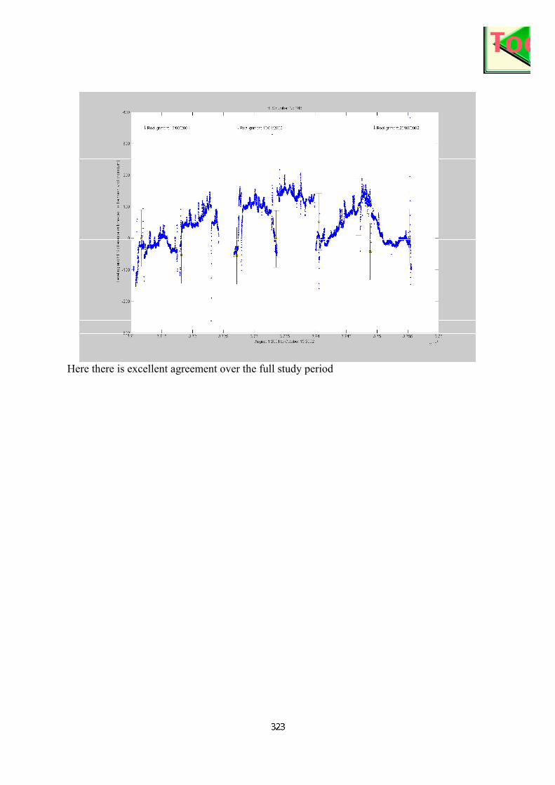
Here there is excellent agreement over the full study period

ANNEX 2 - DEVELOPMENT OF CAPTOR TRIPLETS INSTALLED ON GIRDERS

Measured radial tilt ±1 SD Measured longitudinal tilt ±1

SD

There is actually reasonably good agreement. This girder is installed next to one of the large air-conditioning vents.

There are problems with both the longitudinal and radial tilt.

There is a drift with the radial tilt.

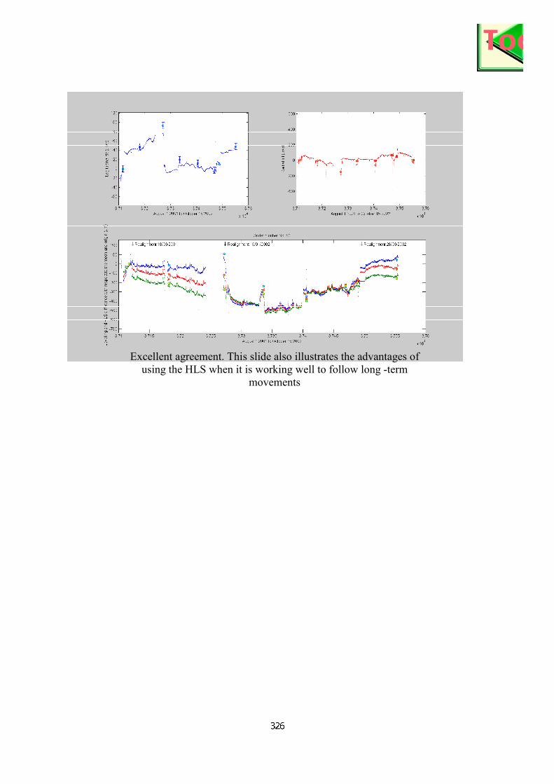
Excellent agreement. This slide also illustrates the advantages of

using the HLS when it is working well to follow long -term movements