The Evolution of Aggregate Stock Ownership:

A Unified Explanation

Kristian Rydqvist Joshua Spizman Ilya Strebulaev∗

September 2008

Abstract

Since World War II, the fraction of stocks owned directly by households has decreasedby more than 50 percentage points in the United States, the United Kingdom, andSweden. We argue that tax policy is the driving force. Using data from eight countries,we show that tax-favored investors have replaced households as stockholders and thatthe fraction of household ownership decreases with measures of the effective marginaltax rate. We further show that the changes in stock ownership accelerate during thehigh-inflation period of the 1970s and the 1980s. These findings are important for policyconsiderations on effective taxation and for financial economics research on the long-term effects of taxation on corporate finance and asset prices.

Keywords: Tax incidence, stock ownership, inflation, pensions.JEL Classification Numbers: G10, G20, H22, H30.

∗We are grateful for data and institutional information from Jyrki Ali-Yrkko of the Research Institute of the FinnishEconomy, Jan Bjuvberg and Leif Muten of the Stockholm School of Economics, Øyvind Bøhren and Dag Michalsen ofthe Norwegian School of Management, John Comisky of the Internal Revenue Service, Shamubeel Eaqub of Goldman& Sachs, Daniel Feenberg of NBER, Bjarne Florentsen of the Copenhagen Business School, Lucien Foldes, CarineGuilbault, Helen Katz, and Arlene Lachapelle of Canada Revenue Agency, Sebastian Herzog of the University ofMannheim, Andrew Jackson of Barclays Global Investors, Lari Kaartinen of the Finnish Central Securities Depository,Matti Kukkonen of the Swedish School of Economics, Matti Keloharju of the Finnish School of Economics andBusiness Administration, Lois Gottlieb of Morneau Sobeco, Riitta Ijas of the Finnish Tax Administration, EilaLaakso of Statistics Finland, Marten Palme of Stockholm University, Chihiro Shima of the Development Bank ofJapan, Sylvie Strobbe of Banque de France, Berouk Terefe of Statistics Canada, Kane Travers of the TaxationStatistics Administration, Daniel Waldenstrom of the Research Institute of Industrial Economics, Per-Olof Westerlundof Forhandlings- och samverkansradet PTK, and Elaine Zimmerman of the Office of Policy & Research. We alsowant to thank Franklin Allen, Andrei Kirilenko, Alan Macnaughton, Jennifer Huang, and seminar participants at theUNC Tax Symposium 2008, Vanderbilt, and Washington Area Finance Association 2008 for suggestions to improvethe paper. Rydqvist: Binghamton University and CEPR; e-mail: rydqvist@binghamton.edu . Spizman: BinghamtonUniversity; email: jspizma1@binghamton.edu . Strebulaev: Stanford University; email: istrebulaev@stanford.edu .

1 Introduction

One of the starkest stylized facts in finance is the decline of households’ direct equity ownership.

In the United States, individuals owned more than 90% of the stock market following World War

II compared to 27% in 2006. Large changes in the stock ownership structure have occurred also

in other countries for which data exist over long time periods. Since World War II, households’

direct ownership has decreased by more than 40 percentage points in the United Kingdom, Sweden

and Finland, and by more than 20 percentage points in Canada, Japan, Germany, and France.

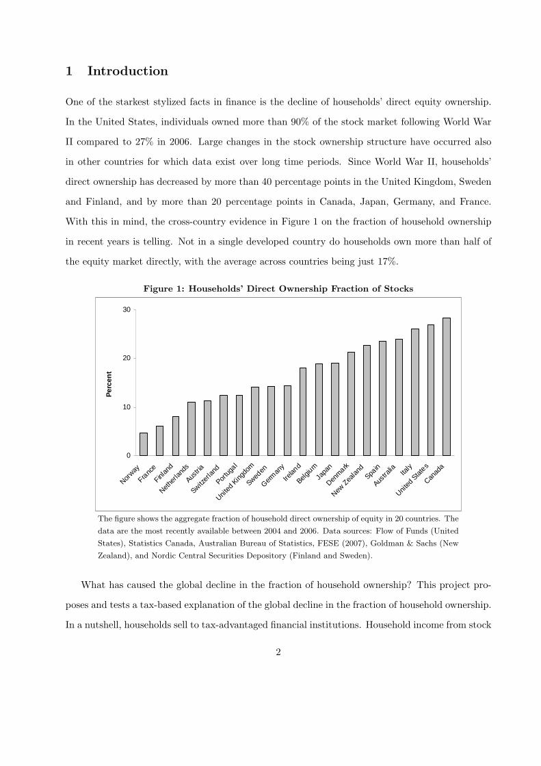
With this in mind, the cross-country evidence in Figure 1 on the fraction of household ownership

in recent years is telling. Not in a single developed country do households own more than half of

the equity market directly, with the average across countries being just 17%.

Figure 1: Households’ Direct Ownership Fraction of Stocks

0

10

20

30

Norway

Franc

e

Finlan

d

Nethe

rland

s

Austria

Switzer

land

Portug

al

Unite

d Kin

gdom

Sweden

Germ

any

Irelan

d

Belgiu

m

Japa

n

Denm

ark

New Z

eala

ndSpa

in

Austra

lia Italy

United

Stat

es

Canad

a

Per

cen

t

The figure shows the aggregate fraction of household direct ownership of equity in 20 countries. The

data are the most recently available between 2004 and 2006. Data sources: Flow of Funds (United

States), Statistics Canada, Australian Bureau of Statistics, FESE (2007), Goldman & Sachs (New

Zealand), and Nordic Central Securities Depository (Finland and Sweden).

What has caused the global decline in the fraction of household ownership? This project pro-

poses and tests a tax-based explanation of the global decline in the fraction of household ownership.

In a nutshell, households sell to tax-advantaged financial institutions. Household income from stock

2

ownership is subject to personal income tax, while financial institutions that manage pension as-

sets can defer income taxes to the time of withdrawal of funds. The principles for the taxation of

pension assets in the United States date back to the Revenue Act of 1926. Similar tax benefits

are granted pension asset management in Canada, United Kingdom, Japan, Germany, Sweden,

and Finland, but the institutional arrangements vary widely from predominantly pension funds

and mutual funds (401(k) plans and Individual Retirement Accounts) in the United States to life

insurance and book reserves in Germany.

Personal income taxes were relatively small before World War II, and the tax advantage of

pensions was relatively insignificant. However, income taxes increased dramatically in the beginning

of World War II creating a strong tax incentive to save for retirement. Interestingly and importantly

for our argument, income taxes remained at high levels after World War II and, in fact, rapidly

increased through the invisible hand of inflation and nominally-fixed tax tables.1 In addition,

households were hurt by inflation through its impact on nominal capital gains taxation. The process

of rising income taxes ended with the Tax Reform Act of 1986 (TRA 1986), the corresponding

tax reforms in the United Kingdom 1988, Canada 1988, Japan 1989, Sweden 1991, and Finland

1993, and the subsequent reduction of world-wide inflation. However, by this point in time, direct

ownership of stocks had largely been replaced by financial institutions and reached the low levels

we see in Figure 1. The combined effects of nominal taxation and inflation appears to have had

the strongest impact on the stock ownership structure in the United Kingdom, which suffered from

severe inflation in the 1970s, and in Sweden and Finland, where citizens were exposed to extreme

levels of taxation in the 1970s and the 1980s. At the other end of the spectrum, the combined

effects of tax and inflation on stock ownership structure appear to be relatively mild in Germany

with tight post-war monetary policy and in Japan with low effective marginal tax rates. The United

States and Canada fall between the two extremes.

The empirical researcher of tax effects encounters several difficulties. First, time-series variation

is primarily associated with a handful of significant tax reforms (the beginning of World War II and1Personal tax tables change infrequently from World War II to the 1970s. Frequent adjustments of personal tax

tables begins 1972 in Canada, 1977 in the United States, United Kingdom, and Finland, and 1979 in Sweden. Formalindexing in the United States begins with the Tax Reform Act of 1986. Germany and Japan do not follow the generalpattern and change their personal tax tables infrequently throughout the post-war period.

3

TRA 1986) and one needs to identify an appropriate source of variation in marginal tax rates (see

Bernheim (2002) for a discussion). We approach this statistical problem by relying on both time-

series and cross-country variation. Hence, we collect detailed historical information on aggregate

equity ownership and tax systems since World War II in eight developed countries. Second, another

empirical issue is to estimate effective as opposed to statutory marginal tax rates. We solve this

problem by constructing a proxy for the effective marginal tax rate from tax tables and GDP-per-

capita time series. For the United States and the United Kingdom, our proxy captures the level

and the dynamics of effective marginal tax rates estimated from tax returns. We show that the rate

of change in the fraction of household ownership is strongly statistically related to the proxy for the

effective marginal tax rate. A third difficulty is to determine the tax status of mutual funds. Income

of mutual funds passes through and gets taxed by the recipient. A tax-based explanation must

therefore show that the indirect stock ownership through a mutual fund income is tax-advantaged

relative to direct stock ownership. Consistent with the tax explanation, we find that the US mutual

fund industry is small and does not begin to grow until the enactment of 401(k) in 1981. We also

estimate that 65% of mutual fund stock portfolios are held in tax-deferred retirement accounts as

of 2006.

The tax mechanism and the resulting current structure of equity ownership have important

implications for both policy and corporate finance research. The role of taxation in shaping fi-

nancial institutions is largely ignored by researchers with the exception of Ippolito (1986) who

labels his argument the tax theory of pensions. In particular, the evidence suggests that not only

the existence of pension funds as we know them (as suggested by Ippolito) but also the existence

and the significance of mutual funds and life insurance companies owe a great deal to the specific

features of the tax code. Thus, the tax mechanism in the United States and the United Kingdom

facilitates a gradual replacement of widely-held direct ownership to widely-held indirect ownership

by financial intermediaries. By the same token, the tax mechanism can potentially explain not only

the portfolio behavior of households but also the transfer of shares to large corporations in some

countries. For example, pension funds in Japan and Sweden are small. Given that corporations

carry pension liabilities on their books, we provide an alternative explanation for the growth of

4

business groups that by the 1980s have come to dominate the financial systems in these countries.

At a more fundamental level, our results add to the ongoing discussion about the origins of

financial systems. LaPorta, Lopez-De-Silanes, Shleifer, and Vishny (1997) claim that financial

institutions are largely determined by static or very slowly changing legal systems while, on the

other hand, Rajan and Zingales (2003) show that countries with less efficient legal systems were

financially well developed in the beginning of the Twentieth Century. Our findings squarely support

the dynamic side of the argument by Rajan and Zingales (2003). Government tax regulation has

shaped financial institutions by creating tax clienteles and leading economic agents to invent ways

to circumvent their tax obligations. This inadvertently has implications for the functioning of the

financial system.

The evidence in Figure 1 casts doubts on the ongoing debate on capital income taxation. As

equity ownership has largely shifted away from households to tax-favored institutions, the economic

effects of manipulating marginal tax rates for households may be relatively small. For example,

the effect of the Jobs and Growth Tax Relief Reconciliation Act of 2003 (JGTRRA) is likely to

be much smaller than predicted.2 Also, a number of important insights on the role of personal

taxation are no longer practical or relevant and a frequently expressed desire of professors to avoid

incorporating personal taxes in their MBA valuation lectures seems to be justified.3 In particular,

the payout puzzle (Black (1976)), why corporations keep paying dividends in lieu of tax-favored

share repurchases, is not a puzzle if shareholders do not pay tax on dividends and capital gains.

Some evidence appears inconsistent with the tax theory. The recent United States evidence

represents an enigma. Even though JGTRRA significantly reduced dividend taxes to the lowest

level since the 1950s, recently we witness an even steeper decline in direct equity ownership than

ever before.

The rest of the paper proceeds as follows. Section 2 presents our evidence on the evolution2See the discussion in Poterba (2004), Julio and Ikenberry (2004), Chaetty and Saez (2005), Brav, Graham,

Harvey, and Michaely (2005).3Classical finance papers that emphasize and study the role of personal income tax include Brennan (1970) (tax-

CAPM), Elton and Gruber (1970) (tax clienteles), Black and Scholes (1974) (cross-section of returns), Black (1976)(payout policy), Miller (1977) (capital structure), and Constanides (1983) (trading strategies). It is important to notethat all these papers are published before TRA 1986 when marginal rates were high and when the household directequity ownership was more significant. Standard MBA textbooks incorporate personal taxation as an important toolin valuation (see e.g. Brealy, Myers, and Allen (2007), Berk and DeMarzo (2007)).

5

of stock ownership and shows the main stylized fact. Section 3 presents the hypothesis and the

methodology. Section 4 discusses personal income tax systems in the sample countries and reports

effective marginal tax rates. Section 5 presents our empirical results, Section 6 discusses alternative

explanations for the results, and Section 7 concludes. The appendix provides details on the tax

rules in each of the sample countries.

2 Evolution of Stock Ownership

The main stylized fact of this paper is a drastic long-term decline of household direct equity

ownership across the globe. We show this by reporting common trends in aggregate stock ownership

in eight developed countries: United States, Japan, United Kingdom, Canada, Germany, France,

Sweden, and Finland. The world market capitalization weights sum up to more than 90%.4

2.1 Ownership Data

The Federal Reserve publishes annual ownership statistics for the United States since 1945 (Flow

of Funds, Table L.213). The ownership shares are reported as fractions of both listed and non-

listed stocks. The Federal Reserve starts with the market value of listed stocks, adds an estimate

of non-listed stocks, eliminates inter-corporate ownership, and subtracts the ownership of finan-

cial institutions. The residual is labeled the “Household sector” and consists of the holdings of

households and non-profit organizations. This methodology means that the US household sector

is upward biased relative to the household sector in most other countries in Figure 1. The bias

arises from including non-listed stocks and non-profit organizations and from eliminating inter-

corporate ownership. The bias from non-listed stocks can be estimated from the difference between

the Flow of Funds total and stock market capitalization, and the ownership of non-profit organi-

zations is available from 1987-2000 (Table L.100a). We have no methodology to assess the bias

from eliminating inter-corporate ownership. Non-listed stocks and non-profit organizations account

for approximately four percentage points each of the household sector in 2006. Consequently, a4According to the World Federation of Exchanges for the year 2005: United States 51%, Japan 23%, United

Kingdom 9%, Canada 4.5%, Germany 3.7%, and Sweden 1.2%. Market capitalization weights for France and Finlandare missing.

6

comparable fraction of household ownership in the United States is 19%. We use the original Flow

of Funds numbers in our analysis below.5

Annual ownership statistics for Canada are available from Statistics Canada since 1961. The

ownership shares are constructed as in the United States except that the total is defined as the book

value of listed and non-listed stocks. A time-series based on market values is under construction and

will be analyzed in a future version of the paper. The household sector is derived as the residual and

consists of actual households and non-profit organizations. Inter-corporate ownership is explicit and

quite small. The percentage difference between total book value and market capitalization of the

Toronto Stock Exchange averages to 26% over 1980-2005. This is a large number and we recompute

the time-series of ownership for Canada. The recomputed fraction of household ownership in 2006

is 29% as shown in Figure 1. In the analysis below, we use the fractions from Statistics Canada

reduced by a time-series constant.

The Tokyo Stock Exchange reports annual ownership statistics for Japan since 1949. The

ownership shares are reported as fractions of the number of shares outstanding before 1970 and

as fractions of market values from 1970. Given that household portfolios tend to be concentrated

to small cap stocks, the aggregate household ownership share in 1949-1970 and the decline in

household ownership over this period is likely to be significantly overestimated. For the United

Kingdom, Germany, France, and Sweden, the ownership shares are fractions of market values. The

sources are listed in the notes of Table 1. Ownership data for the United Kingdom, Sweden, and

Finland are incomplete and only available for some years. The UK ownership statistics are based on

company surveys with the most recent ownership statistics from the share registry. The ownership

statistics from recent years are based on the official share registry in Sweden (since 1975) and

Finland (since 1994). The ownership data from Finland are compiled using a variety of methods.

The first data point from 1958 is based on tax-assessed values, the second data point from 1972 is

based on market values, the data points from 1980-1986 on nominal share values, and the recent

data points on equally-weighted averages of market values. As in Japan, the aggregate household

ownership share since 1980 and the decline in household ownership is likely to be overestimated.5Poterba and Samwick (1995) and French (2008) make attempts to adjust the household sector.

7

2.2 Common Patterns

Table 1 reports the level of stock ownership for six broad investor classes at three points of time:

the earliest available data point, 1990, and the most recent data point. For Japan and Germany,

we choose 1953 as the starting point to eliminate the effects of some initial turbulence shortly after

the war. The table provides several clear patterns.

Household ownership decreases. Column (1) shows that the reduction in the fraction of

household ownership is very large. The difference between the ownership shares in the first and

the third rows in each panel in the table measures how much it falls since World War II. The

equally-weighted average across the eight countries is 39.4%.

Financial institutions ownership increases. The ownership fractions of pension funds, mu-

tual funds, and life insurance companies are shown in columns (2)–(4). The growth in financial

institutions is large. To get a quantitative measure of this long-term growth, we sum across columns

(2)–(4) and take the difference between the sum in the first and the third rows in each panel. The

average difference across the eight countries is 24.2%.

Inter-corporate ownership increases before 1990. Inter-corporate ownership in column (5)

is significant in the countries placed in the bottom of Table 1. The average difference between the

first and the second row in Sweden, Japan, Germany, and Finland is 12.7%. We exclude France

with a relatively short time-series.

Foreign ownership increases after 1990. The foreign ownership fraction is reported in col-

umn (6). Foreign ownership takes off in 1990 after the removal of capital controls (OECD (2002)).

Capital controls in Australia, Canada, Finland, New Zealand, Sweden, and the United Kingdom

were adopted in preparation for or during World War II. Other countries established capital con-

trols in the immediate reconstruction period after the war. Canada removed its capital controls in

1951 and Germany in 1958. United States had capital controls in place during the Vietnam War

(1963–1973). The process of removing capital controls began in the United Kingdom in 1979 and

8

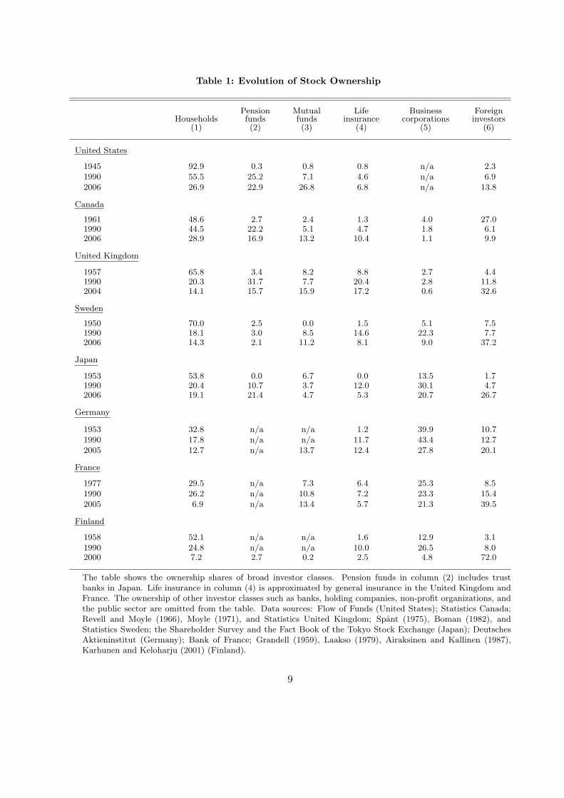
Table 1: Evolution of Stock Ownership

Pension Mutual Life Business ForeignHouseholds funds funds insurance corporations investors

(1) (2) (3) (4) (5) (6)

United States

1945 92.9 0.3 0.8 0.8 n/a 2.31990 55.5 25.2 7.1 4.6 n/a 6.92006 26.9 22.9 26.8 6.8 n/a 13.8

Canada

1961 48.6 2.7 2.4 1.3 4.0 27.01990 44.5 22.2 5.1 4.7 1.8 6.12006 28.9 16.9 13.2 10.4 1.1 9.9

United Kingdom

1957 65.8 3.4 8.2 8.8 2.7 4.41990 20.3 31.7 7.7 20.4 2.8 11.82004 14.1 15.7 15.9 17.2 0.6 32.6

Sweden

1950 70.0 2.5 0.0 1.5 5.1 7.51990 18.1 3.0 8.5 14.6 22.3 7.72006 14.3 2.1 11.2 8.1 9.0 37.2

Japan

1953 53.8 0.0 6.7 0.0 13.5 1.71990 20.4 10.7 3.7 12.0 30.1 4.72006 19.1 21.4 4.7 5.3 20.7 26.7

Germany

1953 32.8 n/a n/a 1.2 39.9 10.71990 17.8 n/a n/a 11.7 43.4 12.72005 12.7 n/a 13.7 12.4 27.8 20.1

France

1977 29.5 n/a 7.3 6.4 25.3 8.51990 26.2 n/a 10.8 7.2 23.3 15.42005 6.9 n/a 13.4 5.7 21.3 39.5

Finland

1958 52.1 n/a n/a 1.6 12.9 3.11990 24.8 n/a n/a 10.0 26.5 8.02000 7.2 2.7 0.2 2.5 4.8 72.0

The table shows the ownership shares of broad investor classes. Pension funds in column (2) includes trustbanks in Japan. Life insurance in column (4) is approximated by general insurance in the United Kingdom andFrance. The ownership of other investor classes such as banks, holding companies, non-profit organizations, andthe public sector are omitted from the table. Data sources: Flow of Funds (United States); Statistics Canada;Revell and Moyle (1966), Moyle (1971), and Statistics United Kingdom; Spant (1975), Boman (1982), andStatistics Sweden; the Shareholder Survey and the Fact Book of the Tokyo Stock Exchange (Japan); DeutschesAktieninstitut (Germany); Bank of France; Grandell (1959), Laakso (1979), Airaksinen and Kallinen (1987),Karhunen and Keloharju (2001) (Finland).

9

continued in Japan 1980, Australia 1983, France 1986, Sweden 1989, Italy and Norway 1990, and

Finland 1991.

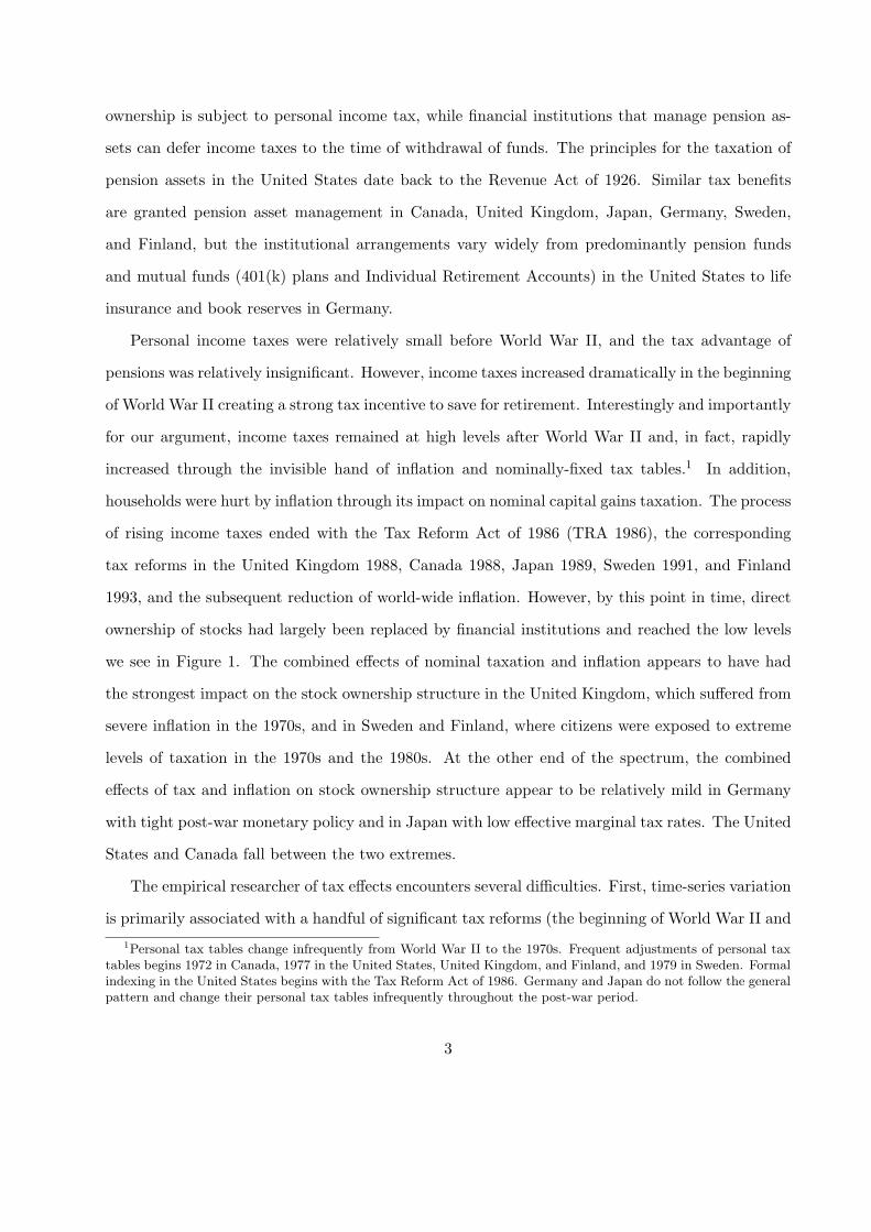
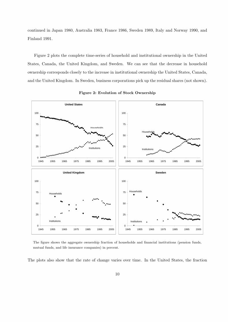
Figure 2 plots the complete time-series of household and institutional ownership in the United

States, Canada, the United Kingdom, and Sweden. We can see that the decrease in household

ownership corresponds closely to the increase in institutional ownership the United States, Canada,

and the United Kingdom. In Sweden, business corporations pick up the residual shares (not shown).

Figure 2: Evolution of Stock Ownership

United States

0

25

50

75

100

1945 1955 1965 1975 1985 1995 2005

Households

Institutions

Canada

0

25

50

75

100

1945 1955 1965 1975 1985 1995 2005

Households

Institutions

United Kingdom

0

25

50

75

100

1945 1955 1965 1975 1985 1995 2005

Households

Institutions

Sweden

0

25

50

75

100

1945 1955 1965 1975 1985 1995 2005

Households

Institutions

The figure shows the aggregate ownership fraction of households and financial institutions (pension funds,

mutual funds, and life insurance companies) in percent.

The plots also show that the rate of change varies over time. In the United States, the fraction

10

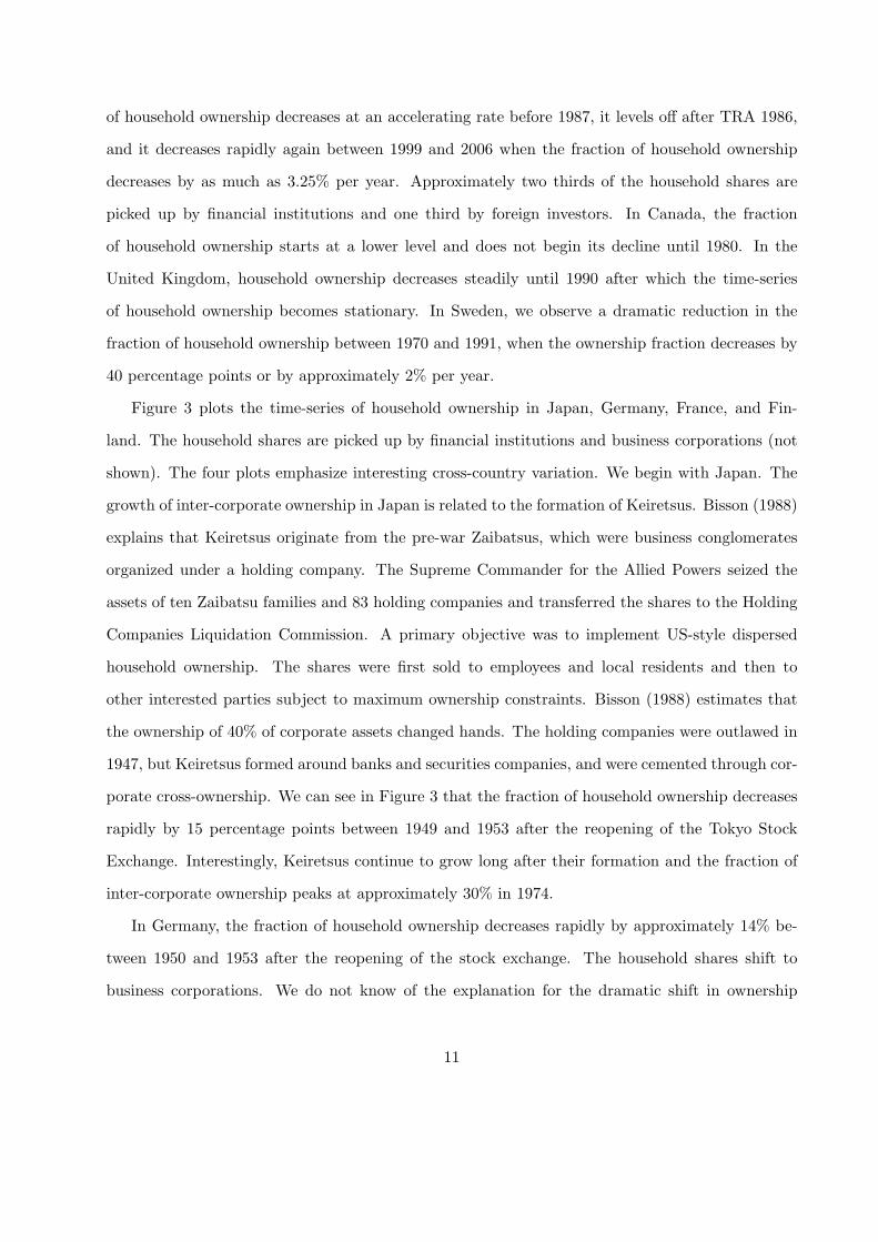
of household ownership decreases at an accelerating rate before 1987, it levels off after TRA 1986,

and it decreases rapidly again between 1999 and 2006 when the fraction of household ownership

decreases by as much as 3.25% per year. Approximately two thirds of the household shares are

picked up by financial institutions and one third by foreign investors. In Canada, the fraction

of household ownership starts at a lower level and does not begin its decline until 1980. In the

United Kingdom, household ownership decreases steadily until 1990 after which the time-series

of household ownership becomes stationary. In Sweden, we observe a dramatic reduction in the

fraction of household ownership between 1970 and 1991, when the ownership fraction decreases by

40 percentage points or by approximately 2% per year.

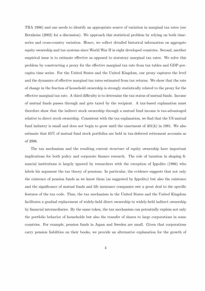
Figure 3 plots the time-series of household ownership in Japan, Germany, France, and Fin-

land. The household shares are picked up by financial institutions and business corporations (not

shown). The four plots emphasize interesting cross-country variation. We begin with Japan. The

growth of inter-corporate ownership in Japan is related to the formation of Keiretsus. Bisson (1988)

explains that Keiretsus originate from the pre-war Zaibatsus, which were business conglomerates

organized under a holding company. The Supreme Commander for the Allied Powers seized the

assets of ten Zaibatsu families and 83 holding companies and transferred the shares to the Holding

Companies Liquidation Commission. A primary objective was to implement US-style dispersed

household ownership. The shares were first sold to employees and local residents and then to

other interested parties subject to maximum ownership constraints. Bisson (1988) estimates that

the ownership of 40% of corporate assets changed hands. The holding companies were outlawed in

1947, but Keiretsus formed around banks and securities companies, and were cemented through cor-

porate cross-ownership. We can see in Figure 3 that the fraction of household ownership decreases

rapidly by 15 percentage points between 1949 and 1953 after the reopening of the Tokyo Stock

Exchange. Interestingly, Keiretsus continue to grow long after their formation and the fraction of

inter-corporate ownership peaks at approximately 30% in 1974.

In Germany, the fraction of household ownership decreases rapidly by approximately 14% be-

tween 1950 and 1953 after the reopening of the stock exchange. The household shares shift to

business corporations. We do not know of the explanation for the dramatic shift in ownership

11

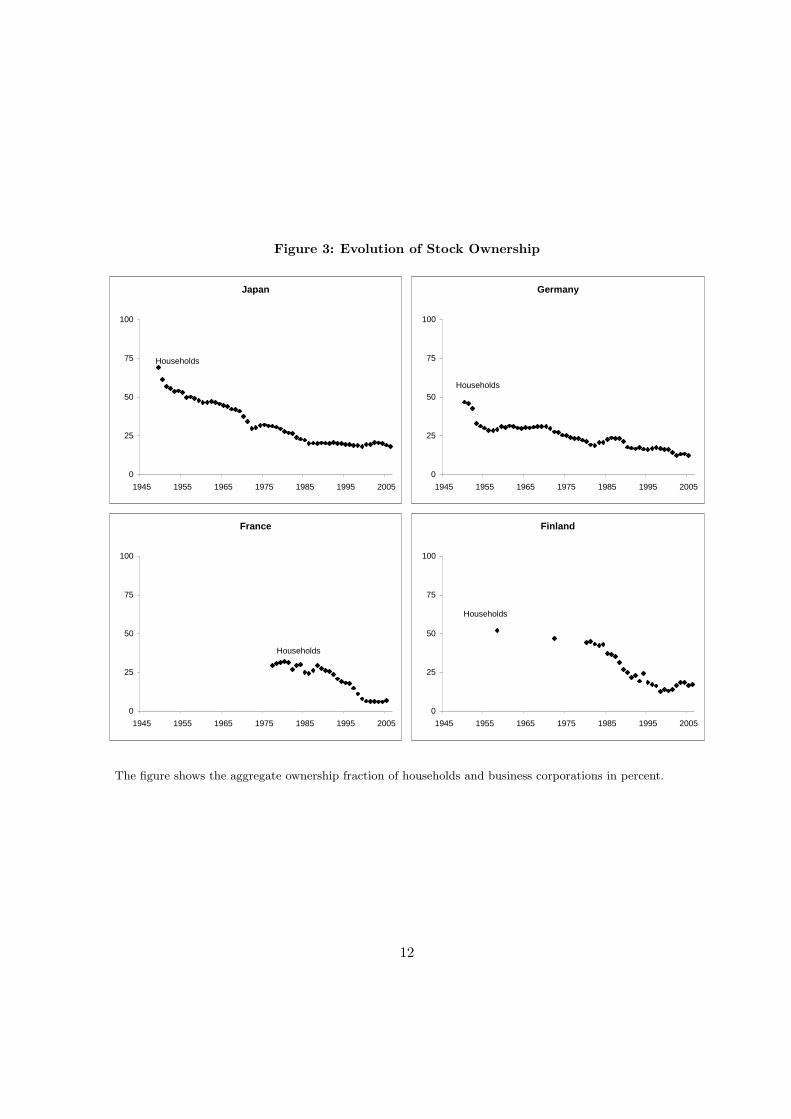
Figure 3: Evolution of Stock Ownership

Japan

0

25

50

75

100

1945 1955 1965 1975 1985 1995 2005

Households

Germany

0

25

50

75

100

1945 1955 1965 1975 1985 1995 2005

Households

Finland

0

25

50

75

100

1945 1955 1965 1975 1985 1995 2005

Households

France

0

25

50

75

100

1945 1955 1965 1975 1985 1995 2005

Households

The figure shows the aggregate ownership fraction of households and business corporations in percent.

12

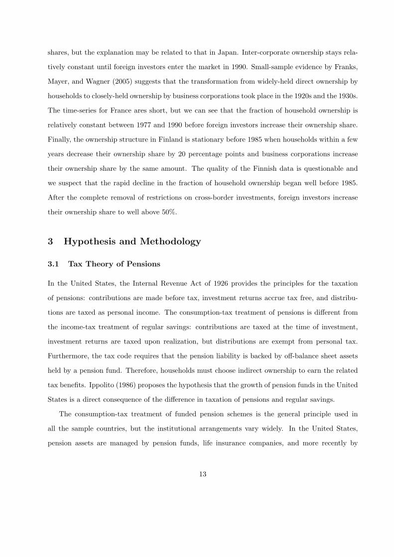
shares, but the explanation may be related to that in Japan. Inter-corporate ownership stays rela-

tively constant until foreign investors enter the market in 1990. Small-sample evidence by Franks,

Mayer, and Wagner (2005) suggests that the transformation from widely-held direct ownership by

households to closely-held ownership by business corporations took place in the 1920s and the 1930s.

The time-series for France ares short, but we can see that the fraction of household ownership is

relatively constant between 1977 and 1990 before foreign investors increase their ownership share.

Finally, the ownership structure in Finland is stationary before 1985 when households within a few

years decrease their ownership share by 20 percentage points and business corporations increase

their ownership share by the same amount. The quality of the Finnish data is questionable and

we suspect that the rapid decline in the fraction of household ownership began well before 1985.

After the complete removal of restrictions on cross-border investments, foreign investors increase

their ownership share to well above 50%.

3 Hypothesis and Methodology

3.1 Tax Theory of Pensions

In the United States, the Internal Revenue Act of 1926 provides the principles for the taxation

of pensions: contributions are made before tax, investment returns accrue tax free, and distribu-

tions are taxed as personal income. The consumption-tax treatment of pensions is different from

the income-tax treatment of regular savings: contributions are taxed at the time of investment,

investment returns are taxed upon realization, but distributions are exempt from personal tax.

Furthermore, the tax code requires that the pension liability is backed by off-balance sheet assets

held by a pension fund. Therefore, households must choose indirect ownership to earn the related

tax benefits. Ippolito (1986) proposes the hypothesis that the growth of pension funds in the United

States is a direct consequence of the difference in taxation of pensions and regular savings.

The consumption-tax treatment of funded pension schemes is the general principle used in

all the sample countries, but the institutional arrangements vary widely. In the United States,

pension assets are managed by pension funds, life insurance companies, and more recently by

13

mutual funds. In Section 6.2, we assess the relative importance of pension and non-pension assets

in US mutual funds. Pension funds and life insurance companies manage significant pension assets

also in Canada, the United Kingdom, and Japan. Japanese pension funds are often managed by

trust banks. Pension funds are small in Germany, France, Sweden, and Finland, where life insurance

companies dominate the pension business. Book reserves also play an important role in Germany,

Japan, and Sweden.

The following stylized setting illustrates the argument. An individual chooses between saving

inside or outside a retirement account. The annual rate of return is r and the time to retirement is

N years.6 Personal income is taxed at rate τ0 when it is earned and at rate τw when it is withdrawn.

Investment returns outside the retirement account are taxed at rate τi, i = 1, ..., N . All taxes are

fixed and known at time 0. Consider the individual who decides to set aside $100 pre-tax money

for retirement. If he invests outside a retirement account, the after-tax payoff after N years equals:

H = [100(1− τ0)]× [1 + r(1− τi)]N . (1)

Equation (1) shows that savings are taxed at rate τ0 when income is earned and at rate τi when

income is reinvested. Hence, household savings outside the retirement account are taxed twice.

Alternatively, if the individual saves inside a retirement account, the after-tax payoff after N years

equals:

P =[100(1 + r)N

]× (1− τw). (2)

Contributions to the retirement account can be made with pre-tax money, investment returns accrue

tax free, and distributions are taxed at rate τw. Hence, savings inside the retirement account are

taxed only once.

Equations (1) and (2) are equal and the individual is indifferent between saving outside or

inside a retirement account if τ0 = τw and τi = 0. This implies that pension savings inside a

retirement account offers two potential tax benefits. First, the individual can benefit from income

smoothing when the tax schedule is progressive and τ0 > τw, i.e., the individual can reduce his6In practice, both future returns and retirement age are uncertain. While we keep them deterministic for simplicity,

our argument can be easily extended to cover uncertainty as we discuss below.

14

life-time tax burden by saving when income is high and withdrawing when income is low. Second,

investment returns inside the retirement account accrue tax free, τi = 0. If we extend the model

with uncertainty and assume that individuals are risk averse, pension savings inside a retirement

account offers the additional advantage of risk sharing with the government: if realized returns are

high, the individual can afford to pay the tax, and if realized returns are low, the tax obligations

are reduced. In other words, a risk-averse investor prefers an uncertain future loss to a certain loss

today.7

For the various reasons outlined above, households have a tax incentive to switch from direct

to indirect ownership. The tax theory of pensions does not say anything about the speed by which

direct ownership is replaced by indirect ownership. There are good reasons to believe that the

process is slow and may well take half a century to complete as suggested by the evidence in Sec-

tion 2 above. First, households can access the tax-advantaged retirement account through payroll

deduction, which by construction is a slow process of building retirement wealth. Since 1975, US

households can also access individual retirement accounts and sell directly-held stocks to finance

IRA contributions, but contribution amounts are limited and with the exception of a short period

in 1982-1986 high-income households are not eligible. Second, assets in a retirement account are

illiquid as they cannot be used for other purposes than retirement. Early withdrawal or borrowing

against the retirement account are subject to penalty. Neither does the theory say that direct

ownership is irrational. There are many other reasons to save than to provide for retirement, and

households may hold stocks for speculation or for incentive reasons (insider ownership). Further-

more, there are investment restrictions and some stocks may not be available inside a retirement

account. For example, the Employee Retirement Income Security Act of 1974 (ERISA) states that

pension funds are subject to the prudent-man rule. Finally, many households may be ignorant

about the relative tax advantage of pensions and react slowly to tax code changes.7In addition, interest rate uncertainty increases the advantage of indirect ownership because P and H are convex

functions.

15

3.2 Empirical Measures

First, we construct a measure of the benefit to avoiding tax on investment income. Equations (1)

and (2) are not directly suitable for empirical testing because they approximate the taxation of

bonds rather than stocks. Therefore, in order to derive an empirical measure, let d be the expected

dividend yield, g the expected capital gain, and let τd and τg be the effective marginal tax rates on

dividends and capital gains, respectively. The expected rate of return from holding stocks inside a

retirement account is:

r = (1 + d)(1 + g)− 1 ≈ d + g, (3)

and the expected rate of return from direct stock ownership outside a retirement account is:

rτ = [1 + d(1− τd)]× [1 + g(1− τg)]− 1 ≈ (1− τd)d + (1− τg)g. (4)

Inflation is central to our analysis and we therefore work with real rates of return. Let i denote the

inflation rate. A simple measure of the relative tax advantage of holding stocks inside a retirement

account is the difference between the real rate of return from holding stocks inside and outside a

retirement account:

GAP =τdd + τgg

1 + i. (5)

Inflation enters the equation through the denominator, but it also enters through the effective

marginal tax rates τd and τg (bracket creep) and through the capital gains growth rate g because

capital gains taxation is nominal. GAP has a dividend and a capital gains component and we will

also examine the explanatory power of each component:

DIVTAX = τd, (6)

and

GAINTAX = τg. (7)

Next, we construct a measure of the benefit to income smoothing. Following Ippolito (1986), we

16

assume certainty, that investors cannot anticipate future changes in the tax code, that income does

not grow over the individual’s life time, and that the risk-free interest rate is zero. Positive interest

and earnings growth would reduce the need for saving and therefore reduce the benefit to income

smoothing, while uncertainty raises it as the demand for pre-cautionary saving increases. We think

our assumptions put an upper boundary on the benefit to income smoothing. An individual begins

contributing to a pension plan at the age of 25, retires at the age of 65, and dies at 78. For

simplicity, we assume that life expectancy is constant and ignore the fact that people live longer

today.8 Let φ be the consumption rate and 1−φ the savings rate. The life-cycle hypothesis means

that the individual chooses the same consumption rate throughout his life time. The individual

works 40 years and needs retirement income 13 years. If the individual pays income tax and makes

regular savings outside a retirement account, his life-time tax liability equals 40 × T (Y ), where

T (·) denotes annual tax liability and Y taxable income. If instead the individual saves inside a

retirement account, he can save pre-tax income and reduce life-time tax liability on earned income

to (40/φ)× T (φY ). A simple measure of the benefit to income smoothing is therefore:

SMOOTH = 1− T (φY)/φ

T (Y). (8)

This variable measures life-time tax savings from income smoothing as a fraction of life-time income

taxes.

3.3 Parameters

The empirical variables derived above require parameter estimates for effective marginal tax rates,

expected stock returns, and inflation. Details about country-specific tax regulations are deferred

to the Appendix.8For example, in the United States, life expectancy conditional on turning 65 years old has increased from 78 to

82 years old between 1950 and 2006.

17

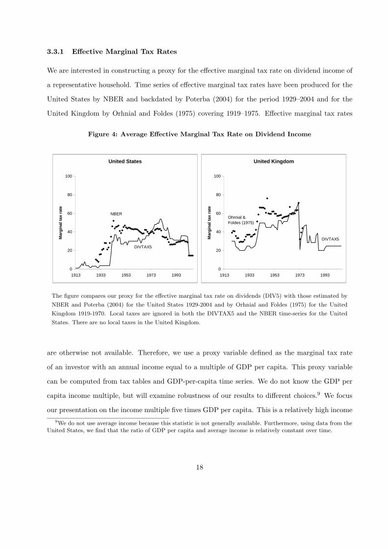
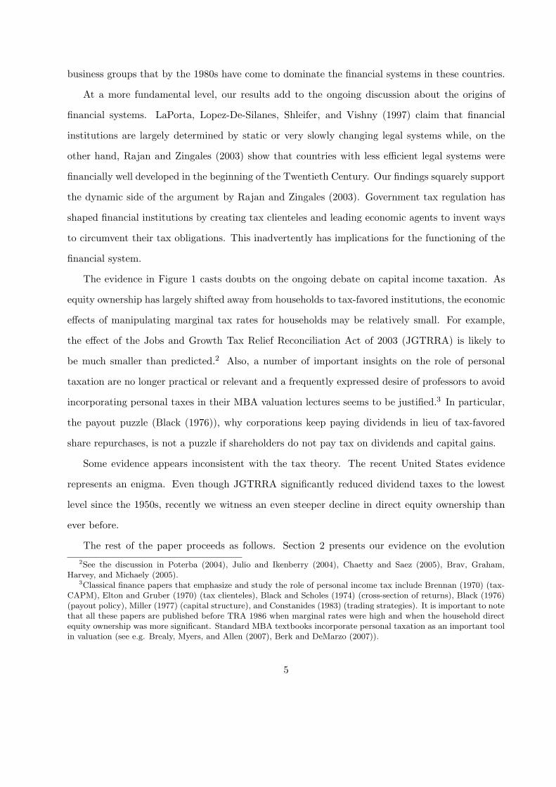
3.3.1 Effective Marginal Tax Rates

We are interested in constructing a proxy for the effective marginal tax rate on dividend income of

a representative household. Time series of effective marginal tax rates have been produced for the

United States by NBER and backdated by Poterba (2004) for the period 1929–2004 and for the

United Kingdom by Orhnial and Foldes (1975) covering 1919–1975. Effective marginal tax rates

Figure 4: Average Effective Marginal Tax Rate on Dividend Income

United States

0

20

40

60

80

100

1913 1933 1953 1973 1993

Mar

gin

al t

ax r

ate

DIVTAX5

NBER

United Kingdom

0

20

40

60

80

100

1913 1933 1953 1973 1993

Mar

gin

al t

ax r

ate

Ohrnial & Foldes (1975)

DIVTAX5

The figure compares our proxy for the effective marginal tax rate on dividends (DIV5) with those estimated by

NBER and Poterba (2004) for the United States 1929-2004 and by Orhnial and Foldes (1975) for the United

Kingdom 1919-1970. Local taxes are ignored in both the DIVTAX5 and the NBER time-series for the United

States. There are no local taxes in the United Kingdom.

are otherwise not available. Therefore, we use a proxy variable defined as the marginal tax rate

of an investor with an annual income equal to a multiple of GDP per capita. This proxy variable

can be computed from tax tables and GDP-per-capita time series. We do not know the GDP per

capita income multiple, but will examine robustness of our results to different choices.9 We focus

our presentation on the income multiple five times GDP per capita. This is a relatively high income9We do not use average income because this statistic is not generally available. Furthermore, using data from the

United States, we find that the ratio of GDP per capita and average income is relatively constant over time.

18

level which reflects our belief that the average stockholder is likely to be a high income earner.10

The associated effective marginal tax rate on dividends at this income level is denoted DIVTAX5.

Figure 4 plots DIVTAX5 against the available time series for the United States and the United

Kingdom. We see that DIVTAX5 is a good proxy for the two time series. It captures the dynamics,

especially the big increase in marginal tax rates at the beginning of World War II and the decrease

after TRA 1986.11 The time-series jump in the United Kingdom when the imputation-tax credit

is introduced in 1973.

There is an interesting, qualitative difference between DIVTAX5 and the other time series.

Focusing on the United States, we can see that DIVTAX5 increases by 26 percentage points, from

28% to 54%, between 1965 and 1980. These changes occur because tax tables are fixed and nominal

growth pushes many households into higher tax brackets. The bracket creep of the 1970s results

in the indexation of tax tables (since 1977), it becomes an important part of Ronald Reagan’s

presidential campaign, and ultimately it results in TRA 1986. The bracket creep is apparent also

in the NBER data. The marginal tax rate of the NBER measure is associated with a drop in the

GDP-per-capita-income multiple from about 12 in 1950 down to about three in 1980. However,

the NBER measure of the marginal tax rate increases by only four percentage points, from 39% to

43%, so DIVTAX5 suggests a more forceful bracket creep than the NBER measure. We believe this

difference can be explained by considering household behavior. DIVTAX5 assumes that households

passively pay their taxes as marginal tax rates increase, while the NBER measure suggests that

high-income households take actions to counter the bracket creep. What is of particular interest

for our study is that households switch from direct to indirect stock ownership. Other actions

may include the purchase of tax-exempt municipal bonds and overconsumption of housing financed

with tax-deductible mortgage debt. Our results below are not sensitive to the measurement error

in DIVTAX5.

Capital gains taxation is markedly different from dividend taxation. First, the statutory tax10This assumption is supported by data from the Survey of Consumer Finances 1998. For example, Poterba (2000)

says that 41% of directly-owned stocks are held by 0.8% of the households.11We have computed sum of squared differences between DIVTAX5 and the other two time series. The sum

of squared differences reaches a minimum at DIVTAX7, but the function is relatively flat between DIVTAX5 andDIVTAX12, so we do not think that DIVTAX7 is better than any close alternative.

19

rate on long-term capital gains is usually lower than the statutory rate on short-term gains and it is

often zero. Second, capital gains tax can be postponed until the stock is sold. The value of deferral

of capital gains has been subject to much debate. Miller (1977) refers to conventional folk wisdom

that 10 years of tax deferral is almost as good as exemption from tax. Bailey (1969) estimates the

value of deferral to 50% of the statutory rate, Protopapadakis (1983) finds estimates in the order

of 25%, and Chay, Choi, and Pontiff (2006) find it to be 55%. Green and Hollifield (2003) model

the advantage of deferral and find numerically that the effective tax rate on capital gains amounts

to approximately 50-60% of the statutory rate. We assume that the effective capital gains tax rate

is 50% of the long-term statutory rate evaluated at various income multiples of GDP per capita.

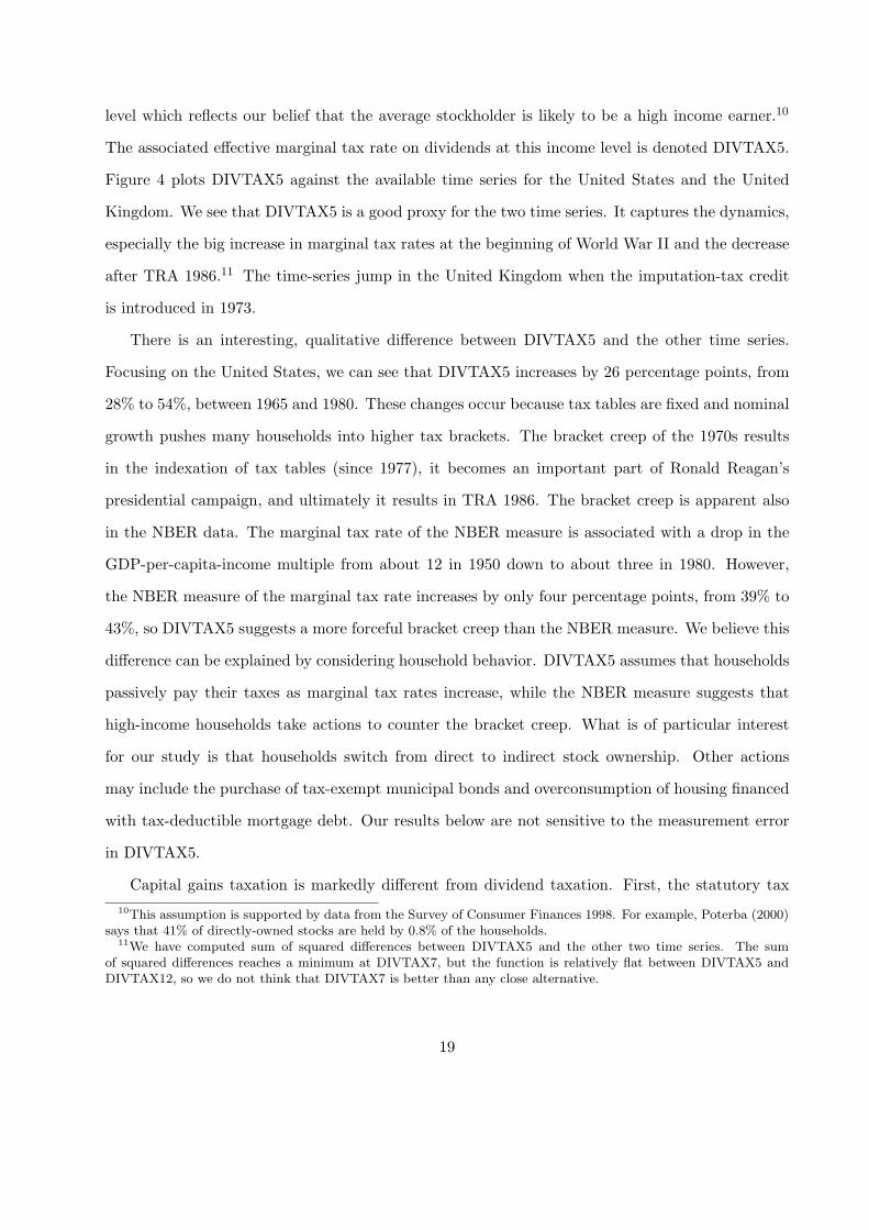
3.3.2 Expected Stock Returns and Inflation

Estimation of expected dividend yield and capital gains rate are intrinsically noisy. We make simple

first-order approximations and pursue a number of robustness checks. Table 2 reports arithmetic

average dividend yields, real GDP growth, and inflation for the seven countries we are interested

in. We assume that the expected dividend yield is d = 4%. A constant dividend yield ignores

Table 2: Parameters

Dividend yield GDP growth Inflation

1950- 1981- 1950- 1973- 1950- 1973- 1991-1980 2006 1972 2006 1972 1990 2006

United States 4.06 2.79 2.80 1.27 2.50 6.64 2.72

Japan 4.75 0.92 8.93 1.58 4.39 5.57 0.38

United Kingdom 5.28 3.90 2.48 2.18 4.29 10.32 2.85

Canada 4.00 2.63 3.27 1.80 2.63 7.35 2.09

Germany 3.31 3.06 6.79 2.12 2.20 3.66 2.07

France 4.63 1.81 5.32 8.26 1.80

Sweden 4.06 2.45 3.38 2.13 4.44 8.63 2.01

Finland 5.93 3.23 4.47 2.50 6.71 9.33 1.64

Average 4.40 2.71 4.57 1.92 4.06 7.47 1.95

The table reports arithmetic averages of macro variables. Data sources: Global Financial Data, InternationalHistorical Statistics.

20

observed variation across countries and well-known structural breaks in the time-series.12 The

low dividend yield in Japan post-1980 is noteworthy and important for our analysis because the

effective marginal tax rate on dividends in Japan depends on the dividend amount from each stock

in the investor’s portfolio. We assume that the expected capital gains rate is 2% plus expected

inflation measured as the three-year moving average. The 2% real growth rate is based on the

evidence of real GDP growth rate in Table 2. These numbers imply that the expected real rate of

return on stocks is approximately 6% before tax, which is within the range reported by Fama and

French (2002) between 1951 and 2000: 4.74% using the dividend growth model and 6.51% using

the earnings growth model.

4 Household Taxation of Stocks

Dividends are taxed as income, but many tax codes offer a dividend-tax relief to reduce the effects

of double taxation of corporate income. Canada introduced a dividend-tax credit in 1949, Japan in

1950, France in 1965, the United Kingdom in 1973, Germany in 1977, and Finland in 1993 under tax

codes which are often referred to as reduced-rate or imputation-tax systems. Furthermore, the tax

codes of Sweden 1991, Finland 1993, United Kingdom 1999, and United States 2003 differentiate

between ordinary income and investment income and subject investment income to lower marginal

tax rates. These tax systems are usually referred to as dual-income systems. The tax code of Japan

1965 combines all of these features: A large dividend from one stock is taxed as ordinary income

subject to a reduced rate, and a small dividend from one stock is taxed as investment income at a

low marginal tax rate.

United States begins taxing capital gains on stocks in 1916. Some other sample countries began

taxing capital gains on stocks relatively late: United Kingdom in 1965, Canada in 1972, and France

in 1976. Sweden begins taxing short-term capital gains in 1910 and Finland in 1920, but long-term

capital gains are tax exempt before 1967 in Sweden and 1986 in Finland. In Germany and Japan,12Substantially lower dividend yields in the United States and the United Kingdom after 1982 can partially be

explained by a dramatic increase in popularity of share repurchases following changes in regulation favoring theserepurchases. Since share repurchases are taxed differently from dividends, we do not add them back in Panel A ofTable 2.

21

long-term capital gains on stocks are effectively tax exempt throughout the time period we study.

4.1 Evolution of Marginal Tax Rates

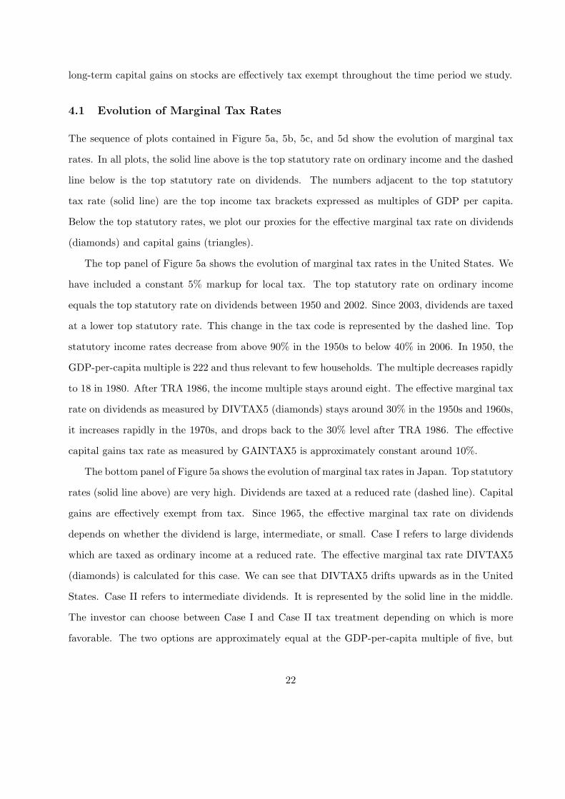
The sequence of plots contained in Figure 5a, 5b, 5c, and 5d show the evolution of marginal tax

rates. In all plots, the solid line above is the top statutory rate on ordinary income and the dashed

line below is the top statutory rate on dividends. The numbers adjacent to the top statutory

tax rate (solid line) are the top income tax brackets expressed as multiples of GDP per capita.

Below the top statutory rates, we plot our proxies for the effective marginal tax rate on dividends

(diamonds) and capital gains (triangles).

The top panel of Figure 5a shows the evolution of marginal tax rates in the United States. We

have included a constant 5% markup for local tax. The top statutory rate on ordinary income

equals the top statutory rate on dividends between 1950 and 2002. Since 2003, dividends are taxed

at a lower top statutory rate. This change in the tax code is represented by the dashed line. Top

statutory income rates decrease from above 90% in the 1950s to below 40% in 2006. In 1950, the

GDP-per-capita multiple is 222 and thus relevant to few households. The multiple decreases rapidly

to 18 in 1980. After TRA 1986, the income multiple stays around eight. The effective marginal tax

rate on dividends as measured by DIVTAX5 (diamonds) stays around 30% in the 1950s and 1960s,

it increases rapidly in the 1970s, and drops back to the 30% level after TRA 1986. The effective

capital gains tax rate as measured by GAINTAX5 is approximately constant around 10%.

The bottom panel of Figure 5a shows the evolution of marginal tax rates in Japan. Top statutory

rates (solid line above) are very high. Dividends are taxed at a reduced rate (dashed line). Capital

gains are effectively exempt from tax. Since 1965, the effective marginal tax rate on dividends

depends on whether the dividend is large, intermediate, or small. Case I refers to large dividends

which are taxed as ordinary income at a reduced rate. The effective marginal tax rate DIVTAX5

(diamonds) is calculated for this case. We can see that DIVTAX5 drifts upwards as in the United

States. Case II refers to intermediate dividends. It is represented by the solid line in the middle.

The investor can choose between Case I and Case II tax treatment depending on which is more

favorable. The two options are approximately equal at the GDP-per-capita multiple of five, but

22

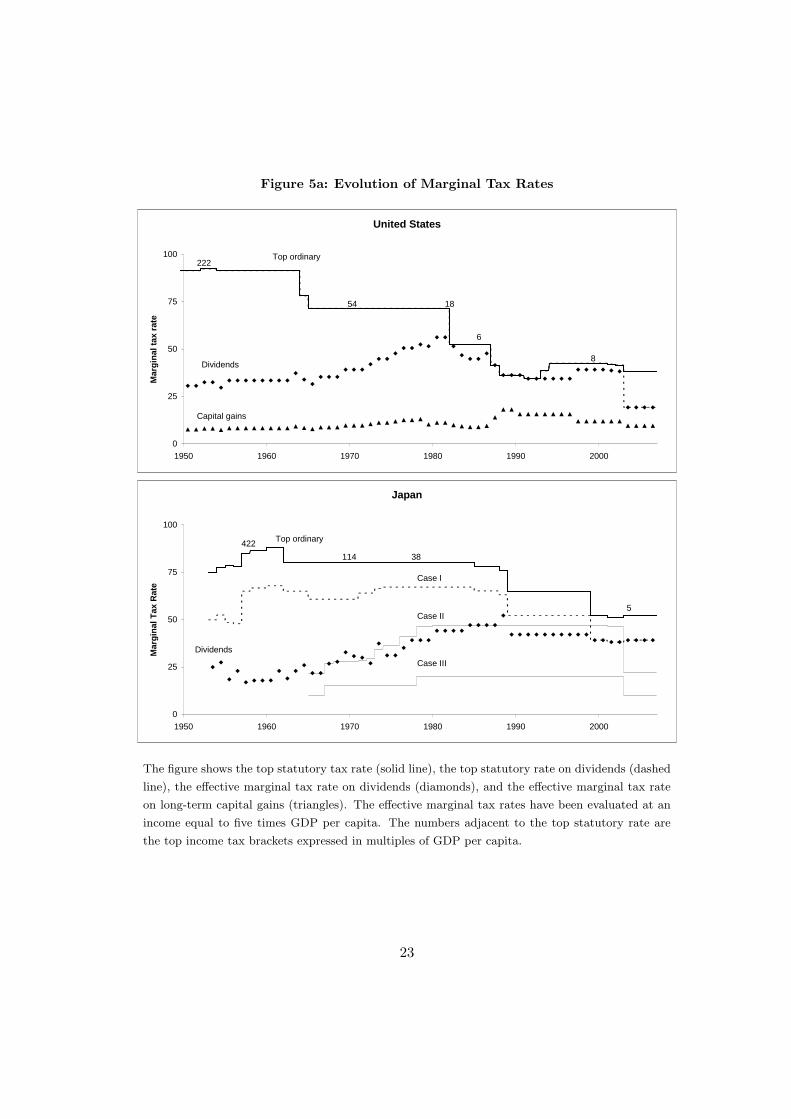
Figure 5a: Evolution of Marginal Tax Rates

United States

0

25

50

75

100

1950 1960 1970 1980 1990 2000

Mar

gin

al t

ax r

ate

Top ordinary

Dividends

Capital gains

222

54 18

6

8

Japan

0

25

50

75

100

1950 1960 1970 1980 1990 2000

Mar

gin

al T

ax R

ate

Top ordinary

Dividends

Case II

Case I

Case III

422

114 38

5

The figure shows the top statutory tax rate (solid line), the top statutory rate on dividends (dashed

line), the effective marginal tax rate on dividends (diamonds), and the effective marginal tax rate

on long-term capital gains (triangles). The effective marginal tax rates have been evaluated at an

income equal to five times GDP per capita. The numbers adjacent to the top statutory rate are

the top income tax brackets expressed in multiples of GDP per capita.

23

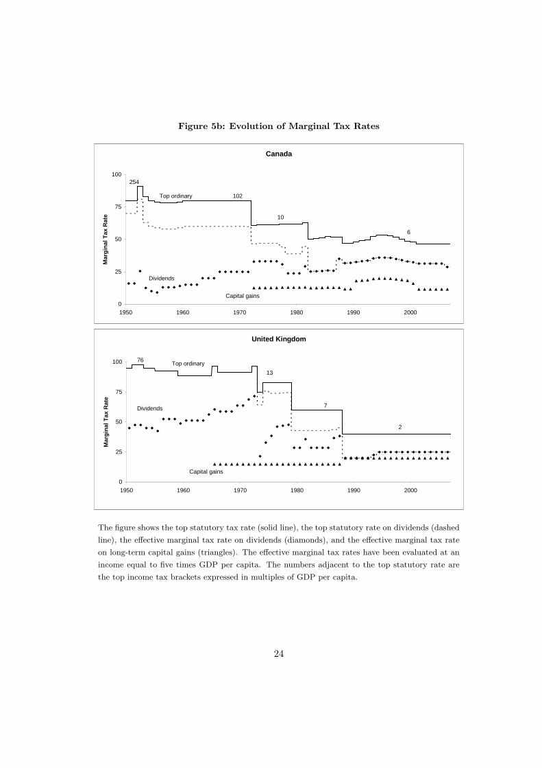
Figure 5b: Evolution of Marginal Tax Rates

Canada

0

25

50

75

100

1950 1960 1970 1980 1990 2000

Mar

gin

al T

ax R

ate

Top ordinary

Dividends

Capital gains

254

102

10

6

United Kingdom

0

25

50

75

100

1950 1960 1970 1980 1990 2000

Mar

gin

al T

ax R

ate

Top ordinary76

13

7

2

Dividends

Capital gains

The figure shows the top statutory tax rate (solid line), the top statutory rate on dividends (dashed

line), the effective marginal tax rate on dividends (diamonds), and the effective marginal tax rate

on long-term capital gains (triangles). The effective marginal tax rates have been evaluated at an

income equal to five times GDP per capita. The numbers adjacent to the top statutory rate are

the top income tax brackets expressed in multiples of GDP per capita.

24

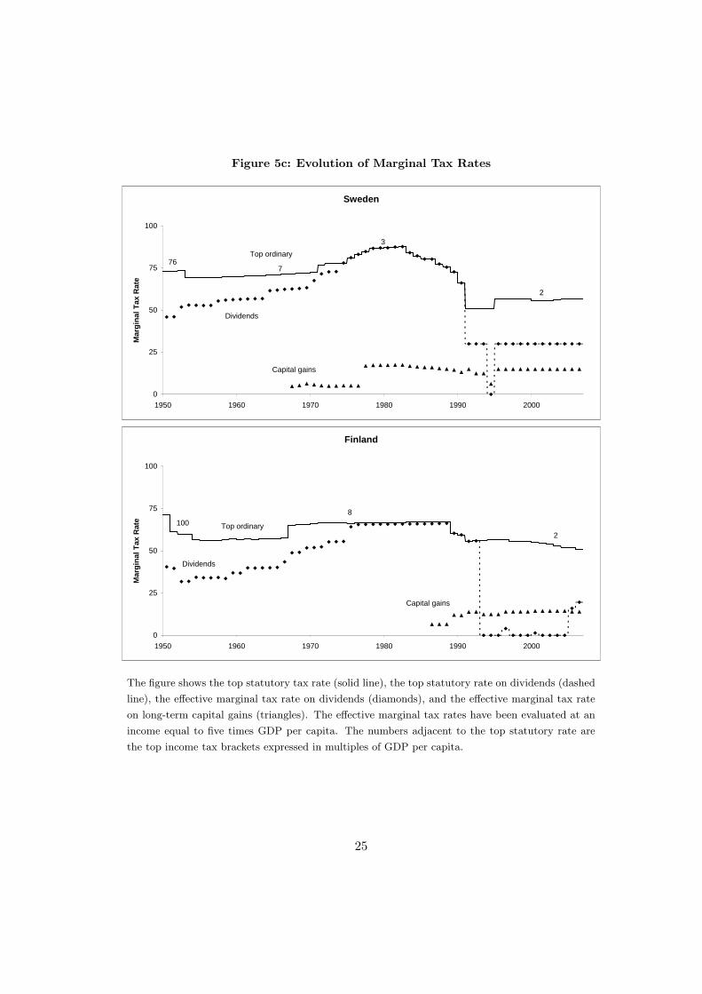
Figure 5c: Evolution of Marginal Tax Rates

Sweden

0

25

50

75

100

1950 1960 1970 1980 1990 2000

Mar

gin

al T

ax R

ate

Top ordinary

Dividends

Capital gains

767

3

2

Finland

0

25

50

75

100

1950 1960 1970 1980 1990 2000

Mar

gin

al T

ax R

ate

Top ordinary

Dividends

Capital gains

1008

2

The figure shows the top statutory tax rate (solid line), the top statutory rate on dividends (dashed

line), the effective marginal tax rate on dividends (diamonds), and the effective marginal tax rate

on long-term capital gains (triangles). The effective marginal tax rates have been evaluated at an

income equal to five times GDP per capita. The numbers adjacent to the top statutory rate are

the top income tax brackets expressed in multiples of GDP per capita.

25

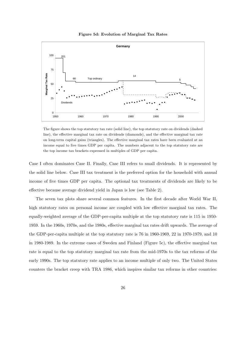
Figure 5d: Evolution of Marginal Tax Rates

Germany

0

25

50

75

100

1950 1960 1970 1980 1990 2000

Mar

gin

al T

ax R

ate

Top ordinary

Dividends

6814

5

201

The figure shows the top statutory tax rate (solid line), the top statutory rate on dividends (dashed

line), the effective marginal tax rate on dividends (diamonds), and the effective marginal tax rate

on long-term capital gains (triangles). The effective marginal tax rates have been evaluated at an

income equal to five times GDP per capita. The numbers adjacent to the top statutory rate are

the top income tax brackets expressed in multiples of GDP per capita.

Case I often dominates Case II. Finally, Case III refers to small dividends. It is represented by

the solid line below. Case III tax treatment is the preferred option for the household with annual

income of five times GDP per capita. The optional tax treatments of dividends are likely to be

effective because average dividend yield in Japan is low (see Table 2).

The seven tax plots share several common features. In the first decade after World War II,

high statutory rates on personal income are coupled with low effective marginal tax rates. The

equally-weighted average of the GDP-per-capita multiple at the top statutory rate is 115 in 1950-

1959. In the 1960s, 1970s, and the 1980s, effective marginal tax rates drift upwards. The average of

the GDP-per-capita multiple at the top statutory rate is 76 in 1960-1969, 22 in 1970-1979, and 10

in 1980-1989. In the extreme cases of Sweden and Finland (Figure 5c), the effective marginal tax

rate is equal to the top statutory marginal tax rate from the mid-1970s to the tax reforms of the

early 1990s. The top statutory rate applies to an income multiple of only two. The United States

counters the bracket creep with TRA 1986, which inspires similar tax reforms in other countries:

26

United Kingdom 1988, Japan 1989, Sweden 1991, and Finland 1993. The corresponding tax reforms

in Canada and Germany, where top statutory rates never exceed 50%, are less pronounced. In all

countries, effective marginal tax rates become equal to top statutory rates after TRA 1986, but top

statutory rates are much lower than in the past.

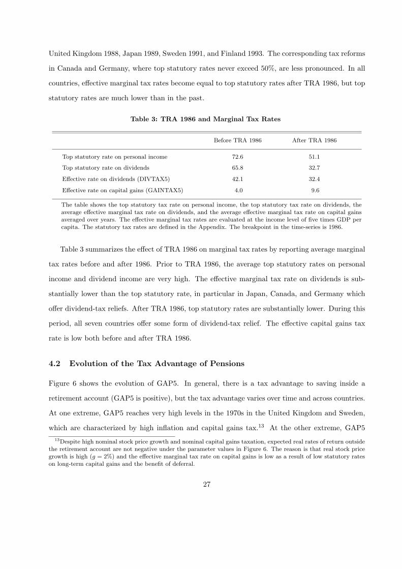
Table 3: TRA 1986 and Marginal Tax Rates

Before TRA 1986 After TRA 1986

Top statutory rate on personal income 72.6 51.1

Top statutory rate on dividends 65.8 32.7

Effective rate on dividends (DIVTAX5) 42.1 32.4

Effective rate on capital gains (GAINTAX5) 4.0 9.6

The table shows the top statutory tax rate on personal income, the top statutory tax rate on dividends, theaverage effective marginal tax rate on dividends, and the average effective marginal tax rate on capital gainsaveraged over years. The effective marginal tax rates are evaluated at the income level of five times GDP percapita. The statutory tax rates are defined in the Appendix. The breakpoint in the time-series is 1986.

Table 3 summarizes the effect of TRA 1986 on marginal tax rates by reporting average marginal

tax rates before and after 1986. Prior to TRA 1986, the average top statutory rates on personal

income and dividend income are very high. The effective marginal tax rate on dividends is sub-

stantially lower than the top statutory rate, in particular in Japan, Canada, and Germany which

offer dividend-tax reliefs. After TRA 1986, top statutory rates are substantially lower. During this

period, all seven countries offer some form of dividend-tax relief. The effective capital gains tax

rate is low both before and after TRA 1986.

4.2 Evolution of the Tax Advantage of Pensions

Figure 6 shows the evolution of GAP5. In general, there is a tax advantage to saving inside a

retirement account (GAP5 is positive), but the tax advantage varies over time and across countries.

At one extreme, GAP5 reaches very high levels in the 1970s in the United Kingdom and Sweden,

which are characterized by high inflation and capital gains tax.13 At the other extreme, GAP513Despite high nominal stock price growth and nominal capital gains taxation, expected real rates of return outside

the retirement account are not negative under the parameter values in Figure 6. The reason is that real stock pricegrowth is high (g = 2%) and the effective marginal tax rate on capital gains is low as a result of low statutory rateson long-term capital gains and the benefit of deferral.

27

is low in Japan and Germany with low inflation and no capital gains tax. The effect of inflation

is visible in the United States where GAP5 peaks in the 1970s before TRA 1986. The effect of

inflation is also visible in Canada, which introduces capital gains tax in 1972 right before inflation

takes off, but the bracket creep is weaker than in the United States because inflation-indexed tax

tables are introduced in 1972.

Figure 6 also illustrates the impact of tax provisions. GAP5 drops after the introduction of

the imputation-tax credit in the United Kingdom 1973 and Germany 1977, and the introduction

of the dual-income systems in Sweden 1991, Finland 1993, and the United States 2003.14 We can

also see that GAP5 jumps after enacting or significantly raising capital gains tax on stocks in the

United Kingdom 1965, Canada 1972, Sweden 1977, and Finland 1986. In the United Kingdom,

GAP5 bounces back when capital gains indexation begins in 1982. We summarize these effects by

regressing GAP5 on dummy variables and expected inflation i:

GAP5 = a0 + a1CREDIT + a2GAIN + a3TRA86 + a4i + e. (9)

CREDIT equals one if the tax code offers a dividend-tax relief and zero otherwise. GAIN equals one

if long-term capital gains are taxed and zero otherwise. For the United Kingdom, GAIN equals zero

when capital gains are indexed between 1982 and 1997. TRA86 equals one after the tax reform

in each country, and zero otherwise: United States 1987, United Kingdom 1988, Japan 1989,

Sweden 1991, and Finland 1993. TRA86 equals zero in Canada and Germany throughout the

sample period. We estimate the regression model (9) with correction for first-order autocorrelation.

The results are reported in the left column of Table 4. All coefficients are large and statistically

significant as visualized by the jumps in Figure 6. A dividend-tax credit reduces GAP5 by 69 basis

points, capital gains tax raises it by 83 basis points, and TRA 1986 reduces GAP5 by 27 basis

points. The effect of inflation is also important. Ten percent expected inflation raises GAP5 by 27

basis points.

Figure 7 shows the benefit to income smoothing. The bracket creep of the 1970s is visible14The spike in the time-series for Sweden 1994 is due to a rapid change in political power in the parliament, which

first removed the dividend tax entirely and then reinstated the dividend tax next year.

28

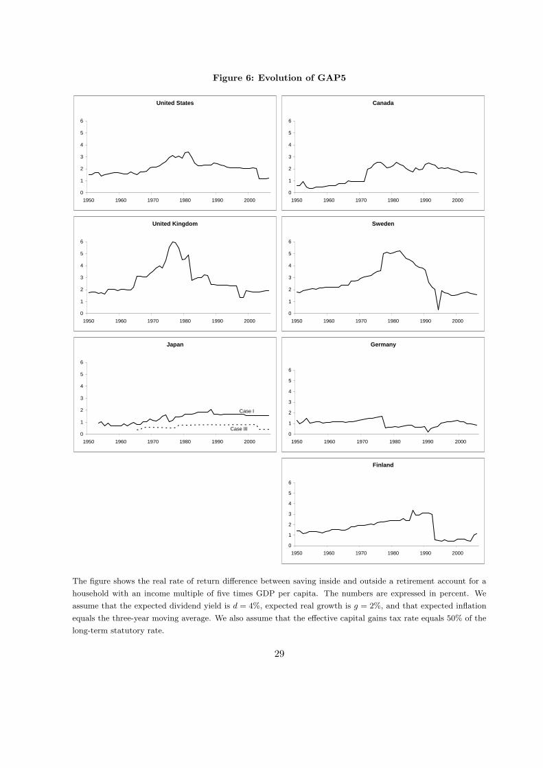
Figure 6: Evolution of GAP5

Canada

0

1

2

3

4

5

6

1950 1960 1970 1980 1990 2000

Sweden

0

1

2

3

4

5

6

1950 1960 1970 1980 1990 2000

United Kingdom

0

1

2

3

4

5

6

1950 1960 1970 1980 1990 2000

United States

0

1

2

3

4

5

6

1950 1960 1970 1980 1990 2000

Germany

0

1

2

3

4

5

6

1950 1960 1970 1980 1990 2000

Finland

0

1

2

3

4

5

6

1950 1960 1970 1980 1990 2000

Japan

0

1

2

3

4

5

6

1950 1960 1970 1980 1990 2000

Case I

Case III

The figure shows the real rate of return difference between saving inside and outside a retirement account for a

household with an income multiple of five times GDP per capita. The numbers are expressed in percent. We

assume that the expected dividend yield is d = 4%, expected real growth is g = 2%, and that expected inflation

equals the three-year moving average. We also assume that the effective capital gains tax rate equals 50% of the

long-term statutory rate.

29

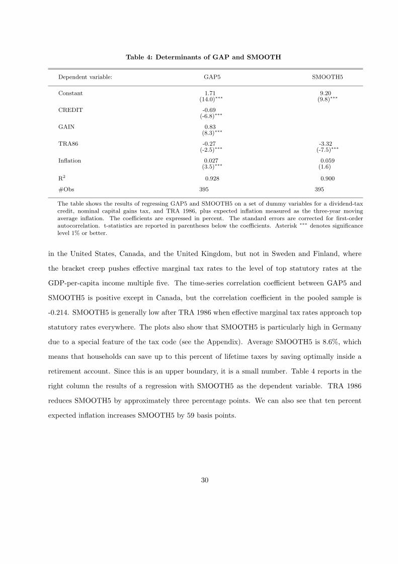
Table 4: Determinants of GAP and SMOOTH

Dependent variable: GAP5 SMOOTH5

Constant 1.71 9.20(14.0)∗∗∗ (9.8)∗∗∗

CREDIT -0.69(-6.8)∗∗∗

GAIN 0.83(8.3)∗∗∗

TRA86 -0.27 -3.32(-2.5)∗∗∗ (-7.5)∗∗∗

Inflation 0.027 0.059(3.5)∗∗∗ (1.6)

R2 0.928 0.900

#Obs 395 395

The table shows the results of regressing GAP5 and SMOOTH5 on a set of dummy variables for a dividend-taxcredit, nominal capital gains tax, and TRA 1986, plus expected inflation measured as the three-year movingaverage inflation. The coefficients are expressed in percent. The standard errors are corrected for first-orderautocorrelation. t-statistics are reported in parentheses below the coefficients. Asterisk ∗∗∗ denotes significancelevel 1% or better.

in the United States, Canada, and the United Kingdom, but not in Sweden and Finland, where

the bracket creep pushes effective marginal tax rates to the level of top statutory rates at the

GDP-per-capita income multiple five. The time-series correlation coefficient between GAP5 and

SMOOTH5 is positive except in Canada, but the correlation coefficient in the pooled sample is

-0.214. SMOOTH5 is generally low after TRA 1986 when effective marginal tax rates approach top

statutory rates everywhere. The plots also show that SMOOTH5 is particularly high in Germany

due to a special feature of the tax code (see the Appendix). Average SMOOTH5 is 8.6%, which

means that households can save up to this percent of lifetime taxes by saving optimally inside a

retirement account. Since this is an upper boundary, it is a small number. Table 4 reports in the

right column the results of a regression with SMOOTH5 as the dependent variable. TRA 1986

reduces SMOOTH5 by approximately three percentage points. We can also see that ten percent

expected inflation increases SMOOTH5 by 59 basis points.

30

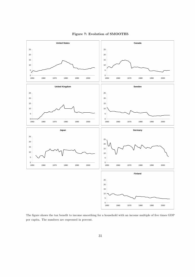
Figure 7: Evolution of SMOOTH5

Canada

0

5

10

15

20

25

1950 1960 1970 1980 1990 2000

Sweden

0

5

10

15

20

25

1950 1960 1970 1980 1990 2000

United Kingdom

0

5

10

15

20

25

1950 1960 1970 1980 1990 2000

United States

0

5

10

15

20

25

1950 1960 1970 1980 1990 2000

Germany

0

5

10

15

20

25

1950 1960 1970 1980 1990 2000

Finland

0

5

10

15

20

25

1950 1960 1970 1980 1990 2000

Japan

0

5

10

15

20

25

1950 1960 1970 1980 1990 2000

The figure shows the tax benefit to income smoothing for a household with an income multiple of five times GDP

per capita. The numbers are expressed in percent.

31

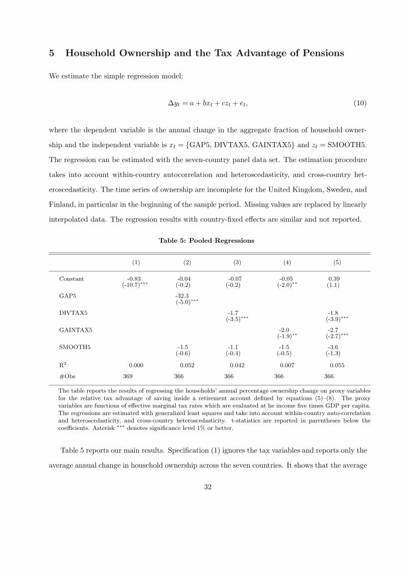
5 Household Ownership and the Tax Advantage of Pensions

We estimate the simple regression model:

∆yt = a + bxt + czt + et, (10)

where the dependent variable is the annual change in the aggregate fraction of household owner-

ship and the independent variable is xt = {GAP5, DIVTAX5, GAINTAX5} and zt = SMOOTH5.

The regression can be estimated with the seven-country panel data set. The estimation procedure

takes into account within-country autocorrelation and heteroscedasticity, and cross-country het-

eroscedasticity. The time series of ownership are incomplete for the United Kingdom, Sweden, and

Finland, in particular in the beginning of the sample period. Missing values are replaced by linearly

interpolated data. The regression results with country-fixed effects are similar and not reported.

Table 5: Pooled Regressions

(1) (2) (3) (4) (5)

Constant -0.83 -0.04 -0.07 -0.05 0.39(-10.7)∗∗∗ (-0.2) (-0.2) (-2.0)∗∗ (1.1)

GAP5 -32.3(-5.0)∗∗∗

DIVTAX5 -1.7 -1.8(-3.5)∗∗∗ (-3.9)∗∗∗

GAINTAX5 -2.0 -2.7(-1.9)∗∗ (-2.7)∗∗∗

SMOOTH5 -1.5 -1.1 -1.5 -3.6(-0.6) (-0.4) (-0.5) (-1.3)

R2 0.000 0.052 0.042 0.007 0.055

#Obs 369 366 366 366 366

The table reports the results of regressing the households’ annual percentage ownership change on proxy variablesfor the relative tax advantage of saving inside a retirement account defined by equations (5)–(8). The proxyvariables are functions of effective marginal tax rates which are evaluated at he income five times GDP per capita.The regressions are estimated with generalized least squares and take into account within-country auto-correlationand heteroscedasticity, and cross-country heteroscedasticity. t-statistics are reported in parentheses below thecoefficients. Asterisk ∗∗∗ denotes significance level 1% or better.

Table 5 reports our main results. Specification (1) ignores the tax variables and reports only the

average annual change in household ownership across the seven countries. It shows that the average

32

annual decline in the fraction of household ownership is 0.83%. Specifications (2)–(5) include the

proxy variables for the relative tax advantage of holding stock inside a retirement account. We can

see that the coefficients of GAP5, DIVTAX5, and GAINTAX5 are significantly different from zero

in all specifications, while the coefficient of SMOOTH5 is not. Once the tax variables GAP5 or

DIVTAX5 are included, the intercept term is not statistically different from zero. The magnitude

of the regression coefficient of GAP5 means that a three percentage point difference between saving

inside and outside a retirement account results in an annual reduction of the fraction of household

ownership of one percentage point. The regression results are very similar and robust to varying

the GDP-per-capita-income multiple from one to 15 because the correlations coefficients are above

80%. The finding that DIVTAX5 and GAINTAX5 have significant explanatory power on their own

means that the choice of parameters for the expected dividend yield, capital gains growth, and

inflation embedded in GAP5 is not critical to our results.

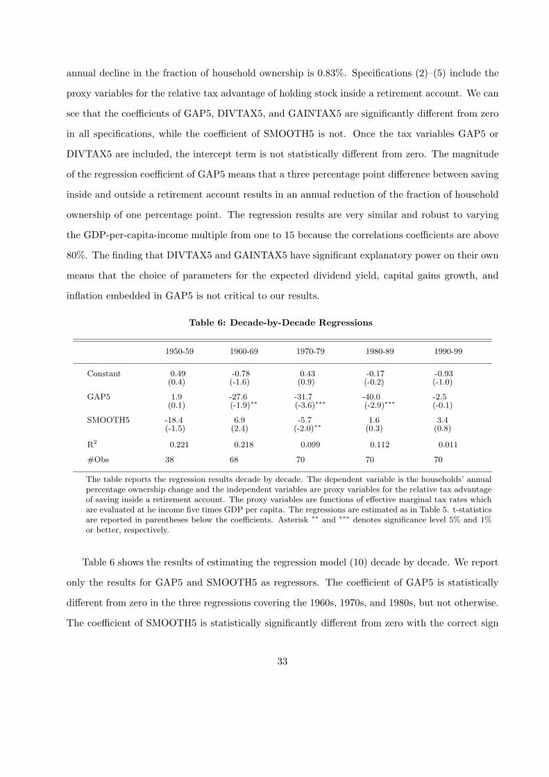
Table 6: Decade-by-Decade Regressions

1950-59 1960-69 1970-79 1980-89 1990-99

Constant 0.49 -0.78 0.43 -0.17 -0.93(0.4) (-1.6) (0.9) (-0.2) (-1.0)

GAP5 1.9 -27.6 -31.7 -40.0 -2.5(0.1) (-1.9)∗∗ (-3.6)∗∗∗ (-2.9)∗∗∗ (-0.1)

SMOOTH5 -18.4 6.9 -5.7 1.6 3.4(-1.5) (2.4) (-2.0)∗∗ (0.3) (0.8)

R2 0.221 0.218 0.099 0.112 0.011

#Obs 38 68 70 70 70

The table reports the regression results decade by decade. The dependent variable is the households’ annualpercentage ownership change and the independent variables are proxy variables for the relative tax advantageof saving inside a retirement account. The proxy variables are functions of effective marginal tax rates whichare evaluated at he income five times GDP per capita. The regressions are estimated as in Table 5. t-statisticsare reported in parentheses below the coefficients. Asterisk ∗∗ and ∗∗∗ denotes significance level 5% and 1%or better, respectively.

Table 6 shows the results of estimating the regression model (10) decade by decade. We report

only the results for GAP5 and SMOOTH5 as regressors. The coefficient of GAP5 is statistically

different from zero in the three regressions covering the 1960s, 1970s, and 1980s, but not otherwise.

The coefficient of SMOOTH5 is statistically significantly different from zero with the correct sign

33

in the 1970s, but not otherwise. These regression results demonstrate that significant explanatory

power of the regression model is due to cross-section variation in effective marginal tax rates. The

regression results also emphasize the interaction between tax and inflation before TRA 1986. The

lack of explanatory power in the 1990s suggests that TRA 1986 and related tax reforms in other

countries successfully responded to the bracket creep.

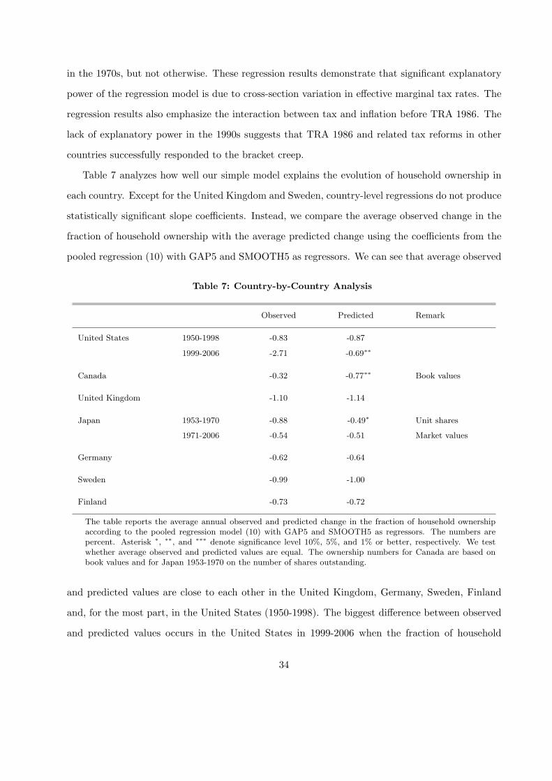
Table 7 analyzes how well our simple model explains the evolution of household ownership in

each country. Except for the United Kingdom and Sweden, country-level regressions do not produce

statistically significant slope coefficients. Instead, we compare the average observed change in the

fraction of household ownership with the average predicted change using the coefficients from the

pooled regression (10) with GAP5 and SMOOTH5 as regressors. We can see that average observed

Table 7: Country-by-Country Analysis

Observed Predicted Remark

United States 1950-1998 -0.83 -0.87

1999-2006 -2.71 -0.69∗∗

Canada -0.32 -0.77∗∗ Book values

United Kingdom -1.10 -1.14

Japan 1953-1970 -0.88 -0.49∗ Unit shares

1971-2006 -0.54 -0.51 Market values

Germany -0.62 -0.64

Sweden -0.99 -1.00

Finland -0.73 -0.72

The table reports the average annual observed and predicted change in the fraction of household ownershipaccording to the pooled regression model (10) with GAP5 and SMOOTH5 as regressors. The numbers arepercent. Asterisk ∗, ∗∗, and ∗∗∗ denote significance level 10%, 5%, and 1% or better, respectively. We testwhether average observed and predicted values are equal. The ownership numbers for Canada are based onbook values and for Japan 1953-1970 on the number of shares outstanding.

and predicted values are close to each other in the United Kingdom, Germany, Sweden, Finland

and, for the most part, in the United States (1950-1998). The biggest difference between observed

and predicted values occurs in the United States in 1999-2006 when the fraction of household

34

ownership decreases much faster than predicted. In Japan, the fraction of household ownership

decreases faster than predicted before 1970 when ownership is reported as fractions of the number

of shares outstanding. We suspect that this is due to data error. If households are over-weighted in

small capitalization stocks, the starting point at 69% household ownership in 1949 is overestimated.

Furthermore, if households chose randomly among small and large cap stocks when they sell, the

observed annual decrease in household ownership is also overestimated. From 1970-2006, when the

Japanese ownership data are based on market values, the regression model performs well. The

deviation between observed and predicted values in Canada may also be due to data error because

the household ownership fraction is derived from book values.

6 Alternative Explanations

6.1 Omitted Variables

The literature identifies many non-tax reasons for the growth of pension funds, mutual funds, and

inter-corporate ownership. For example, Bernheim (2002) says that the tax benefits of private

pension plans do not imply that “the growth of the pension system is exclusively, or even primarily

attributable to the tax system.” Private pension plans may work as screening devices or incentive

schemes. Furthermore, Allen and Santomero (1998) argue that mutual funds and other financial

intermediaries generate risk sharing services beyond that of providing a well-diversified stock port-

folio at low cost. Specifically, the cost of executing a trade has decreased over time, as evidenced by

the evolution of trading volume, and should therefore reduce the demand for financial intermedia-

tion. Instead, they propose that the opportunity cost of time of wealthy individuals, referred to as

participation costs, has increased over time, thereby generating demand for intermediation services.

In the same vein, Friedman (1996) discusses how intermediation may improve all the stock market’s

basic functions: capital allocation and accumulation, risk sharing, liquidity, and price discovery.

He also argues that intermediation may reduce the separation of ownership and control. Finally,

the common explanation for inter-corporate ownership and the growth of business groups in Japan

and Germany is related to information-based theories of internal capital markets and their ability

35

to raise more money and make better allocation decisions than the external capital market (see

Stein (2003) for a survey).

All of these theories may contribute to explaining the general time trend in household own-

ership and, since we cannot quantify information-based variables such as screening, incentives,

participation costs, or agency costs, we cannot rule out any of the alternative explanations for the

decreasing fraction of household ownership. However, the alternative explanations are silent about

the correlations with our proxy variables for effective marginal tax rates. Any of the alternative

explanations faces a challenge to explain the specific cross-country paths that we observe.

We have deliberately omitted several variables that may influence households’ savings decisions.

For example, we ignore the possible crowding-out effect of mandatory public pension plans, as well

as regulatory limits on either contributions to or benefits from private pension plans. Public pen-

sions are important for low-income households but less significant for high-income households with

direct ownership of stocks. Contribution limits to employer-sponsored pension plans are generous

in all the sample countries because retirement accounts cannot be used for other purposes than re-

tirement (Ippolito (1986)). In Sweden, the tax code supports the centrally-negotiated contributions

to private pension plans. It is well known that average contributions to IRAs and Keogh plans in

the United States and to RRSPs in Canada are well below statutory maxima.

Savings decisions are also related to demographic variables such as increasing life expectancy

and the baby boom effect. People who live longer have an incentive to save more. Life expectancy

is a slowly-increasing variable and we capture its possible impact through the regression constant.

The baby boom can be measured as the proportion of the population between 50 and 59 years old.

In the United States, this variable is approximately constant around 10% from 1950 to the mid

1990s when it shoots up and reaches 13% in 2006. This path is statistically significantly correlated

with the change in household ownership in the United States, but the variable follows very different

paths in the countries on the loosing side of the war. In Japan, the variable is constantly increasing

and in Germany it is cyclical. In the pooled sample, the proportion of the population in their fifties

has no explanatory power on its own and the explanatory power of the tax variables are unaffected

by including it in the regression.

36

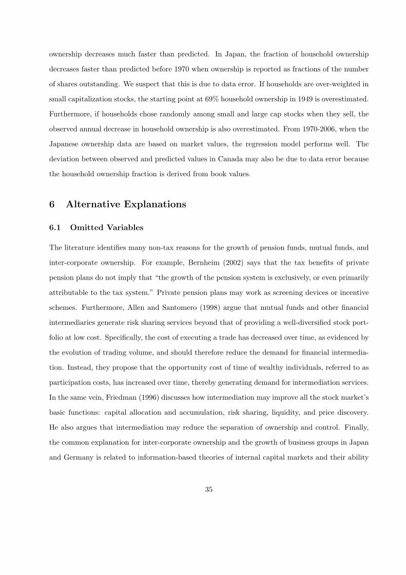
6.2 Tax Position of US Mutual Funds

The general principle for mutual funds is pass-through tax treatment, which means that the tax

status of mutual fund assets depends on the tax position of their owners. In this section, we argue

that US mutual funds manage mostly tax-deferred assets in either 401(k)-type defined contribution

plans or Individual Retirement Accounts (IRAs). The plan balances of 401(k) plans and IRAs

Figure 8: Stock Ownership of U.S. Mutual Funds and Pension Funds

Pension Funds: Stocks

0

5

10

15

20

25

1945 1955 1965 1975 1985 1995 2005

Ow

ner

ship

fra

ctio

n Private

Public

Mutual Funds: Stocks

0

5

10

15

20

25

1945 1955 1965 1975 1985 1995 2005

Ow

ner

ship

fra

ctio

n

401(k) + IRA

Pension Funds:Bonds

0

3

6

9

12

15

1945 1955 1965 1975 1985 1995 2005

Ow

ner

ship

fra

ctio

n

Public

Private

Mutual Funds: Bonds

0

3

6

9

12

15

1945 1955 1965 1975 1985 1995 2005

Ow

ner

ship

fra

ctio

n

401(k) + IRA

The top two figures show the stock ownership fractions in percent of private and public pension funds and of

mutual funds, and the bottom two figures show the respective ownership shares of taxable bond s (treasury,

corporate, and agency debt). The figures for mutual fund ownership shares also mark the introduction of 401(k)

plans in 1982 and the universally eligible Individual Retirement Account. Source: Flow of Funds.

are approximately equally large and mutual funds manage 50% of each (Investment Company

37

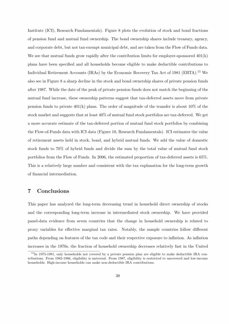
Institute (ICI), Research Fundamentals). Figure 8 plots the evolution of stock and bond fractions

of pension fund and mutual fund ownership. The bond ownership shares include treasury, agency,

and corporate debt, but not tax-exempt municipal debt, and are taken from the Flow of Funds data.

We see that mutual funds grow rapidly after the contribution limits for employer-sponsored 401(k)

plans have been specified and all households become eligible to make deductible contributions to

Individual Retirement Accounts (IRAs) by the Economic Recovery Tax Act of 1981 (ERTA).15 We

also see in Figure 8 a sharp decline in the stock and bond ownership shares of private pension funds

after 1987. While the date of the peak of private pension funds does not match the beginning of the

mutual fund increase, these ownership patterns suggest that tax-deferred assets move from private

pension funds to private 401(k) plans. The order of magnitude of the transfer is about 10% of the

stock market and suggests that at least 40% of mutual fund stock portfolios are tax-deferred. We get

a more accurate estimate of the tax-deferred portion of mutual fund stock portfolios by combining

the Flow-of-Funds data with ICI data (Figure 10, Research Fundamentals). ICI estimates the value

of retirement assets held in stock, bond, and hybrid mutual funds. We add the value of domestic

stock funds to 70% of hybrid funds and divide the sum by the total value of mutual fund stock

portfolios from the Flow of Funds. In 2006, the estimated proportion of tax-deferred assets is 65%.

This is a relatively large number and consistent with the tax explanation for the long-term growth

of financial intermediation.

7 Conclusions

This paper has analyzed the long-term decreasing trend in household direct ownership of stocks

and the corresponding long-term increase in intermediated stock ownership. We have provided

panel-data evidence from seven countries that the change in household ownership is related to

proxy variables for effective marginal tax rates. Notably, the sample countries follow different

paths depending on features of the tax code and their respective exposure to inflation. As inflation

increases in the 1970s, the fraction of household ownership decreases relatively fast in the United15In 1975-1981, only households not covered by a private pension plan are eligible to make deductible IRA con-

tributions. From 1982-1986, eligibility is universal. From 1987, eligibility is restricted to uncovered and low-incomehouseholds. High-income households can make non-deductible IRA contributions.

38

Kingdom and Sweden where there are high effective marginal tax rates and capital gains stocks are

taxed. At the same time, the fraction of household ownership decreases slowly in Germany with

tight monetary policy and Japan with low effective marginal tax rates and no capital gains tax on

stocks. The other countries, the United States, Canada, and Finland fall between the extremes.

These findings lead to a number of important research and policy implications.

First, the ending ownership structure with mostly intermediated stock ownership and relatively

little direct ownership by individuals is a consequence of tax policy. Specifically, the stock ownership

shares of pension funds, mutual funds, and life insurance companies would have been much smaller

without the tax benefits granted to pensions. In some ways, the tax explanation trivializes the role

of financial intermediaries; they are important because the tax maker wants them. Diversification

services, transaction costs, monitoring, and other explanations that have been suggested to explain

the role of intermediaries may be less important.

Second, the rules for the taxation of private pensions in the United States date far back to the

beginning of the Twentieth Century. Similar tax rules govern pensions also in the other sample

countries. One obvious intention of tax policy is to is to stimulate intermediated private savings.

Hence, we conclude that tax policy has been successful. Presumably, stock prices would have been

much lower without the tax benefits awarded to pensions.

Third, we have argued that inflation matters to stock ownership through its impact on effective

marginal tax rates and by imposing tax liability on nominal capital gains. We find that the two

effects are approximately equally important. In retrospect, we conclude that the United Kingdom,

Canada, Sweden, and Finland poorly timed capital gains taxation on stocks, while Canada, Ger-

many, and United Kingdom successfully timed the introduction of dividend-tax credit. In Canada

and United Kingdom the effects of the two tax reforms partly offset each other. We also find that

the TRA 1986 and subsequent tax reforms in other countries have been successful in combatting

inflation by reducing effective marginal tax rates and by indexing personal tax tables.

Finally, John Maynard Keynes writes: There is no subtler, no surer means of overturning the

existing basis of society than to debauch the currency. The process engages all the hidden forces

of economic law on the side of destruction, and it does it in the manner which not one man in a

39

million is able to diagnose. The destruction of households’ direct ownership of stocks appears to

be another surprising consequence of inflation.

40

References

Airaksinen, T., and T. Kallinen, 1987, Yhteisoomistus ja ristiinomistus suomalaisissa suuryrityk-sissa, working paper, Research Institute of the Finnish Economy.

Allen, Franklin, and Anthony M. Santomero, 1998, The Theory of Financial Intermediation, Journalof Banking and Finance 21, 1461–1485.

Bailey, Martin J., 1969, Capital Gains and Income Taxation, in Arnold C. Harberger and MartinJ. Bailey, eds.: The Taxation of Income from Capital (The Brookings Institution, WashingtonD.C.).

Bell, Leonie, and Tim Jenkinson, 2002, New Evidence on the Impact of Dividend Taxation and onthe Identity of the Marginal Investor, Journal of Finance 57, 1321–1346.

Berk, Jonathan, and Peter DeMarzo, 2007, Corporate Finance. (Pearson Addison Wesley).

Bernheim, Douglas, 2002, Taxation and Saving, in Alan J. Auerbach and Martin Feldstein, eds.:Handbooks of Public Finance (Elsevier Science B.V.).

Bisson, Thomas A., 1988, Zaibatsu Dissolution in Japan. (University of California Press).

Black, Fischer, 1976, The Dividend Puzzle, Journal of Portfolio Management 2, 5–8.

Black, Fisher, and Myron Scholes, 1974, The Effects of Dividend Yield and Dividend Policy onCommon Stock Prices and Returns, Journal of Financial Economics 1, 1–22.

Boman, Ragnar, 1982, Agarstrukturen i borsforetagen. (Statens offentliga utredningar (SOU)1982:28 Stockholm).

Booth, Laurence D., and David J. Johnston, 1984, The Ex-Dividend Day Behavior of CanadianStock Prices: Tax Changes and Clientele Effects, Journal of Finance 39, 457–476.

Borsch-Supan, Axel, 1994, Savings in Germany—Part I: Incentives, in James M. Poterba, ed.:Public Policies and Household Saving (University of Chicago Press).

Brav, Alon, John R. Graham, Campbell R. Harvey, and Roni Michaely, 2005, Payout Policy in the21st Century, Journal of Financial Economics 77, 483–527.

Brealy, Richard A., Stewart C. Myers, and Franklin Allen, 2007, Principles of Corporate Finance.(McGraw-Hill Irwin).

Brennan, Michael J., 1970, Taxes, Market Valuation and Corporate Financial Policy, National TaxJournal 23, 417–427.

Chaetty, Raj, and Emmanuel Saez, 2005, Dividend Taxes and Corporate Behavior: Evidence fromthe 2003 Dividend Tax Cut, Quarterly Journal of Economics 120, 791–833.

Chay, J.B., Dosoung Choi, and Jeffrey Pontiff, 2006, Market Valuation of Tax-Timing Options:Evidence from Capital Gains Distributions, Journal of Finance 61, 837–866.

41

Constanides, George M., 1983, Capital Market Equilibrium with Personal Tax, Econometrica 51,611–636.

Corneo, Giacomo, 2005, The Rise and Likely Fall of the German Income Tax, 1958-2005, CESifoEconomic Studies 51, 159–186.

Elton, Edwin J., and Martin J. Gruber, 1970, Marginal Stockholders Tax Rates and the ClienteleEffect, Review of Economics and Statistics 52, 68–74.

Fama, Eugene F., and Kenneth R. French, 2002, The Equity Premium, Journal of Finance 57,637–660.

FESE, 2007, Share Ownership Structure in Europe, Federation of European Securities Exchanges.

Franks, Julian, Colin Mayer, and Hannes F. Wagner, 2005, The Origins of the GermanCorporation—Finance, Ownership and Control, working paper SSRN.

French, Kenneth R., 2008, The Cost of Active Investing, working paper Dartmouth College.

Friedman, Benjamin M., 1996, Economics Implications of Changing Share Ownership, Journal ofPortfolio Management 22, 59–70.

Grandell, Axel, 1959, Aktiesparande, working paper, Swedish School of Economics (Abo Akademi).

Green, Richard C., and Burton Hollifield, 2003, The Personal-Tax Advantages of Equity, Journalof Financial Economics 67, 175–216.

Ippolito, Richard A., 1986, Pensions, Economics, and Public Policy. (Dow Jones-Irwin HomewoodIllinois).

Ishi, Hiromitsu, 2001, The Japanese Tax System. (Oxford University Press).

Julio, Brandon, and David Ikenberry, 2004, Reappearing Dividends, Journal of Applied CorporateFinance 16, 89–100.

Karhunen, Jussi, and Matti Keloharju, 2001, Shareownership on Finland 2000, Finnish Journal ofBusiness Economics 50, 188–226.

King, Mervyn A., 1977, Public Policy and the Corporation. (John Wiley & Sons New York).

Kukkonen, Matti, 2000, Capital Gains Taxation and Realization Behaviour: Evidence from FinnishPanel Data, Dissertation Helsinki School of Economics and Business Administration.

Laakso, J., 1979, Osake, obligaatio ja porssi, working paper, Helsinki School of Economics.

Lakonishok, Joseph, and Theo Vermaelen, 1983, Tax Reform and Ex-Dividend Day Behavior,Journal of Finance 38, 1157–1179.

LaPorta, Rafael, Florencio Lopez-De-Silanes, Andrei Shleifer, and Robert W. Vishny, 1997, LegalDeterminants of External Finance, Journal of Finance 52, 1131–1150.

Miller, Merton H., 1977, Debt and Taxes, Journal of Finance 32, 261–275.

42

Moyle, John, 1971, The Pattern of Ordinary Share Ownership. (Cambridge University Press).

OECD, 2002, Forty Years’ Experience with the OECD Code of Liberalisation of Capital Movements.(OECD, Paris).

Orhnial, A. J. H., and L. P. Foldes, 1975, Estimates of Marginal Tax Rates fro Dividends and BondInterest in the United Kingdom 1991-1970, Economica 42, 79–91.

Perry, J. Harvey, 1989, A Fiscal History of Canada—The Postwar Years. (Canadian Tax Founda-tion Toronto).

Perry, J. Harvey, 1990, Taxation in Canada. (Canadian Tax Foundation Toronto).

Poterba, James, 2000, Stock Market Wealth and Consumption, Journal of Economic Perspectives14, 99–118.

Poterba, James, 2004, Taxation and Corporate Payout Policy, American Economic Review 94,171–175.

Poterba, James M., and Andrew A. Samwick, 1995, Stock Ownership Patterns, Stock MarketFluctuations, and Consumption, BROOK 1995, 295–372.

Protopapadakis, Aris, 1983, Some Indirect Evidence on Effective Capital Gains Tax Rates, Journalof Business 56, 127–138.

Rajan, Raghuram G., and Luigi Zingales, 2003, The great reversals: the politics of financial devel-opment in the twentieth century, Journal of Financial Economics 69, 5–50.

Revell, Jack, and John Moyle, 1966, The Owners of Quoted Ordinary Shares—A Survey for 1963.(Chapman and Hall Ltd London).

Soderberg, Hans, 1996, Inkomstskattens utveckling under 1900-talet. En vagvisare for skatte-berakningar aren 1921-1996. (Skattebetalarnas forening Stockholm).

Spant, Roland, 1975, Formogenhetsfordelningen i Sverige. (Prisma Stockholm).

Stein, Jeremy C., 2003, Agency, Information, and Corporate Investment, in George M. Constan-tinides and Milton Harris and Rene M. Stulz, eds., Handbook of the Economics of Finance—Volume 1A, Corporate Finance, Elsevier North-Holland.

43

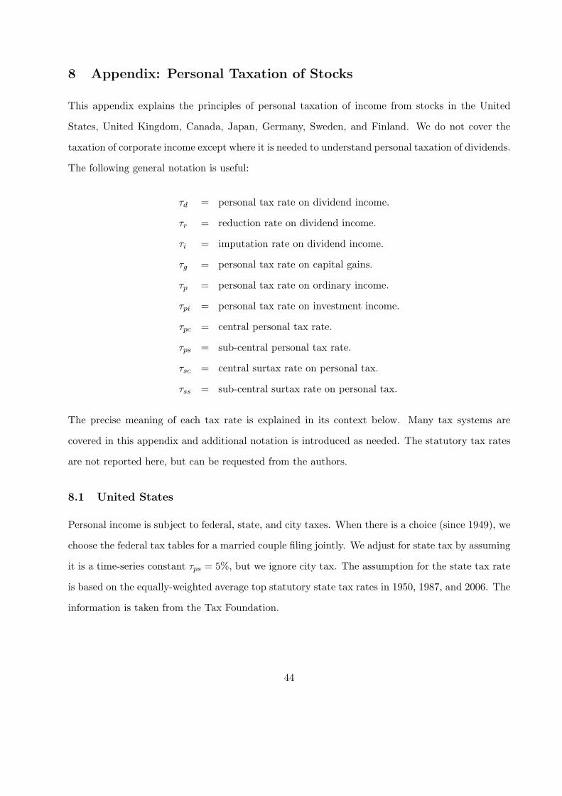
8 Appendix: Personal Taxation of Stocks

This appendix explains the principles of personal taxation of income from stocks in the United

States, United Kingdom, Canada, Japan, Germany, Sweden, and Finland. We do not cover the

taxation of corporate income except where it is needed to understand personal taxation of dividends.

The following general notation is useful:

τd = personal tax rate on dividend income.

τr = reduction rate on dividend income.

τi = imputation rate on dividend income.

τg = personal tax rate on capital gains.

τp = personal tax rate on ordinary income.

τpi = personal tax rate on investment income.

τpc = central personal tax rate.

τps = sub-central personal tax rate.

τsc = central surtax rate on personal tax.

τss = sub-central surtax rate on personal tax.

The precise meaning of each tax rate is explained in its context below. Many tax systems are

covered in this appendix and additional notation is introduced as needed. The statutory tax rates

are not reported here, but can be requested from the authors.

8.1 United States

Personal income is subject to federal, state, and city taxes. When there is a choice (since 1949), we

choose the federal tax tables for a married couple filing jointly. We adjust for state tax by assuming

it is a time-series constant τps = 5%, but we ignore city tax. The assumption for the state tax rate

is based on the equally-weighted average top statutory state tax rates in 1950, 1987, and 2006. The

information is taken from the Tax Foundation.

44

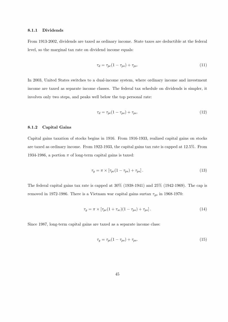
8.1.1 Dividends

From 1913-2002, dividends are taxed as ordinary income. State taxes are deductible at the federal

level, so the marginal tax rate on dividend income equals:

τd = τpc(1− τps) + τps. (11)

In 2003, United States switches to a dual-income system, where ordinary income and investment

income are taxed as separate income classes. The federal tax schedule on dividends is simpler, it

involves only two steps, and peaks well below the top personal rate:

τd = τpi(1− τps) + τps. (12)

8.1.2 Capital Gains

Capital gains taxation of stocks begins in 1916. From 1916-1933, realized capital gains on stocks

are taxed as ordinary income. From 1922-1933, the capital gains tax rate is capped at 12.5%. From

1934-1986, a portion π of long-term capital gains is taxed:

τg = π × [τpc(1− τps) + τps] . (13)

The federal capital gains tax rate is capped at 30% (1938-1941) and 25% (1942-1969). The cap is

removed in 1972-1986. There is a Vietnam war capital gains surtax τgs in 1968-1970:

τg = π × [τpc(1 + τsc)(1− τps) + τps] . (14)

Since 1987, long-term capital gains are taxed as a separate income class:

τg = τpi(1− τps) + τps. (15)

45

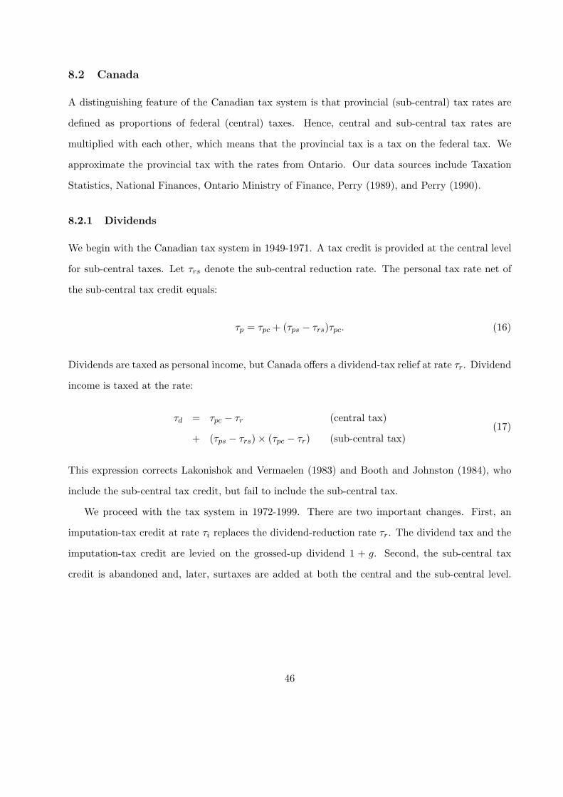
8.2 Canada

A distinguishing feature of the Canadian tax system is that provincial (sub-central) tax rates are

defined as proportions of federal (central) taxes. Hence, central and sub-central tax rates are

multiplied with each other, which means that the provincial tax is a tax on the federal tax. We

approximate the provincial tax with the rates from Ontario. Our data sources include Taxation

Statistics, National Finances, Ontario Ministry of Finance, Perry (1989), and Perry (1990).

8.2.1 Dividends

We begin with the Canadian tax system in 1949-1971. A tax credit is provided at the central level

for sub-central taxes. Let τrs denote the sub-central reduction rate. The personal tax rate net of

the sub-central tax credit equals:

τp = τpc + (τps − τrs)τpc. (16)

Dividends are taxed as personal income, but Canada offers a dividend-tax relief at rate τr. Dividend

income is taxed at the rate:

τd = τpc − τr (central tax)

+ (τps − τrs)× (τpc − τr) (sub-central tax)(17)

This expression corrects Lakonishok and Vermaelen (1983) and Booth and Johnston (1984), who

include the sub-central tax credit, but fail to include the sub-central tax.

We proceed with the tax system in 1972-1999. There are two important changes. First, an

imputation-tax credit at rate τi replaces the dividend-reduction rate τr. The dividend tax and the

imputation-tax credit are levied on the grossed-up dividend 1 + g. Second, the sub-central tax

credit is abandoned and, later, surtaxes are added at both the central and the sub-central level.

46

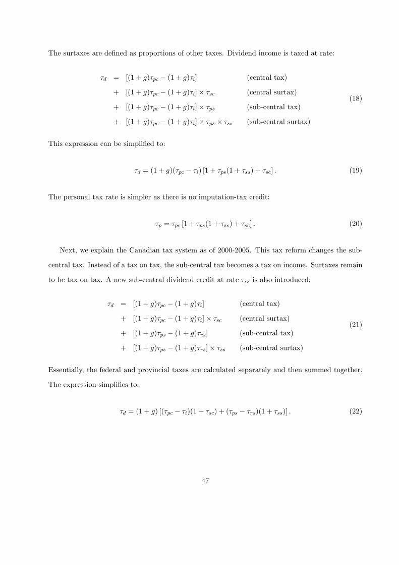
The surtaxes are defined as proportions of other taxes. Dividend income is taxed at rate:

τd = [(1 + g)τpc − (1 + g)τi] (central tax)

+ [(1 + g)τpc − (1 + g)τi]× τsc (central surtax)

+ [(1 + g)τpc − (1 + g)τi]× τps (sub-central tax)

+ [(1 + g)τpc − (1 + g)τi]× τps × τss (sub-central surtax)

(18)

This expression can be simplified to:

τd = (1 + g)(τpc − τi) [1 + τps(1 + τss) + τsc] . (19)

The personal tax rate is simpler as there is no imputation-tax credit:

τp = τpc [1 + τps(1 + τss) + τsc] . (20)

Next, we explain the Canadian tax system as of 2000-2005. This tax reform changes the sub-

central tax. Instead of a tax on tax, the sub-central tax becomes a tax on income. Surtaxes remain

to be tax on tax. A new sub-central dividend credit at rate τrs is also introduced:

τd = [(1 + g)τpc − (1 + g)τi] (central tax)

+ [(1 + g)τpc − (1 + g)τi]× τsc (central surtax)

+ [(1 + g)τps − (1 + g)τrs] (sub-central tax)

+ [(1 + g)τps − (1 + g)τrs]× τss (sub-central surtax)

(21)

Essentially, the federal and provincial taxes are calculated separately and then summed together.

The expression simplifies to:

τd = (1 + g) [(τpc − τi)(1 + τsc) + (τps − τrs)(1 + τss)] . (22)

47

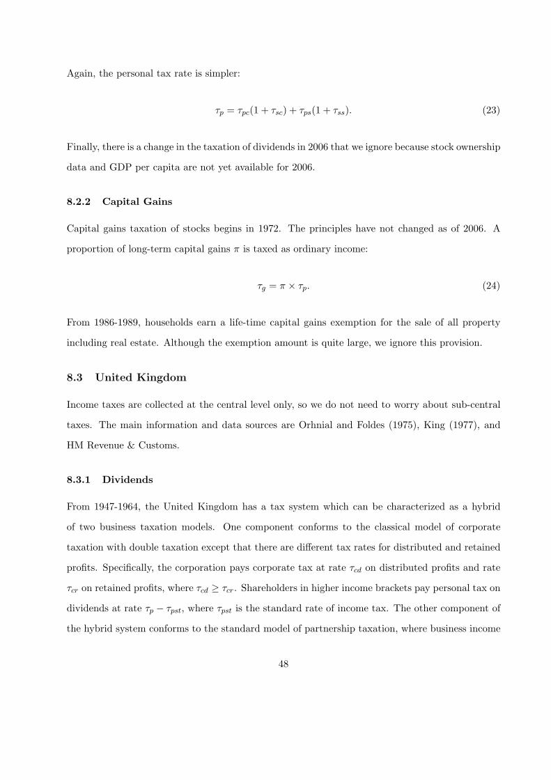
Again, the personal tax rate is simpler:

τp = τpc(1 + τsc) + τps(1 + τss). (23)

Finally, there is a change in the taxation of dividends in 2006 that we ignore because stock ownership

data and GDP per capita are not yet available for 2006.

8.2.2 Capital Gains

Capital gains taxation of stocks begins in 1972. The principles have not changed as of 2006. A

proportion of long-term capital gains π is taxed as ordinary income:

τg = π × τp. (24)

From 1986-1989, households earn a life-time capital gains exemption for the sale of all property

including real estate. Although the exemption amount is quite large, we ignore this provision.

8.3 United Kingdom

Income taxes are collected at the central level only, so we do not need to worry about sub-central

taxes. The main information and data sources are Orhnial and Foldes (1975), King (1977), and

HM Revenue & Customs.

8.3.1 Dividends

From 1947-1964, the United Kingdom has a tax system which can be characterized as a hybrid

of two business taxation models. One component conforms to the classical model of corporate

taxation with double taxation except that there are different tax rates for distributed and retained

profits. Specifically, the corporation pays corporate tax at rate τcd on distributed profits and rate

τcr on retained profits, where τcd ≥ τcr. Shareholders in higher income brackets pay personal tax on

dividends at rate τp − τpst, where τpst is the standard rate of income tax. The other component of

the hybrid system conforms to the standard model of partnership taxation, where business income

48

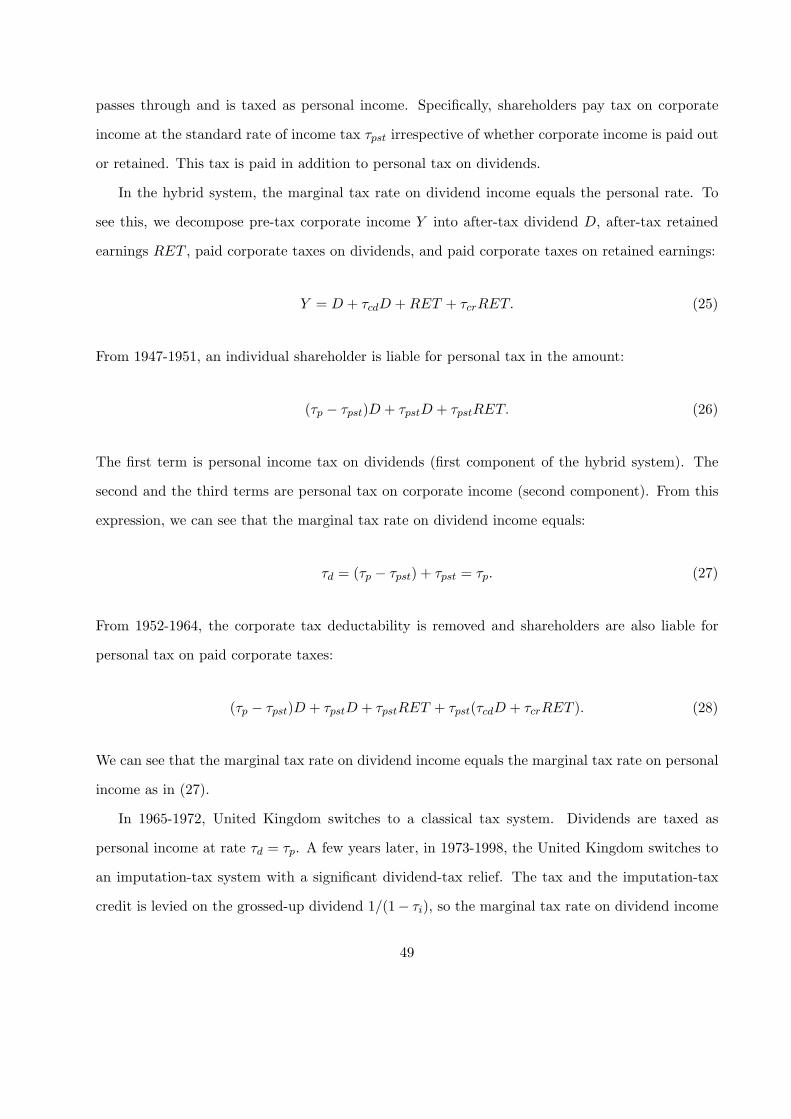
passes through and is taxed as personal income. Specifically, shareholders pay tax on corporate

income at the standard rate of income tax τpst irrespective of whether corporate income is paid out

or retained. This tax is paid in addition to personal tax on dividends.

In the hybrid system, the marginal tax rate on dividend income equals the personal rate. To

see this, we decompose pre-tax corporate income Y into after-tax dividend D, after-tax retained

earnings RET , paid corporate taxes on dividends, and paid corporate taxes on retained earnings:

Y = D + τcdD + RET + τcrRET. (25)

From 1947-1951, an individual shareholder is liable for personal tax in the amount:

(τp − τpst)D + τpstD + τpstRET. (26)

The first term is personal income tax on dividends (first component of the hybrid system). The

second and the third terms are personal tax on corporate income (second component). From this

expression, we can see that the marginal tax rate on dividend income equals:

τd = (τp − τpst) + τpst = τp. (27)

From 1952-1964, the corporate tax deductability is removed and shareholders are also liable for

personal tax on paid corporate taxes:

(τp − τpst)D + τpstD + τpstRET + τpst(τcdD + τcrRET ). (28)

We can see that the marginal tax rate on dividend income equals the marginal tax rate on personal

income as in (27).

In 1965-1972, United Kingdom switches to a classical tax system. Dividends are taxed as

personal income at rate τd = τp. A few years later, in 1973-1998, the United Kingdom switches to

an imputation-tax system with a significant dividend-tax relief. The tax and the imputation-tax

credit is levied on the grossed-up dividend 1/(1− τi), so the marginal tax rate on dividend income

49

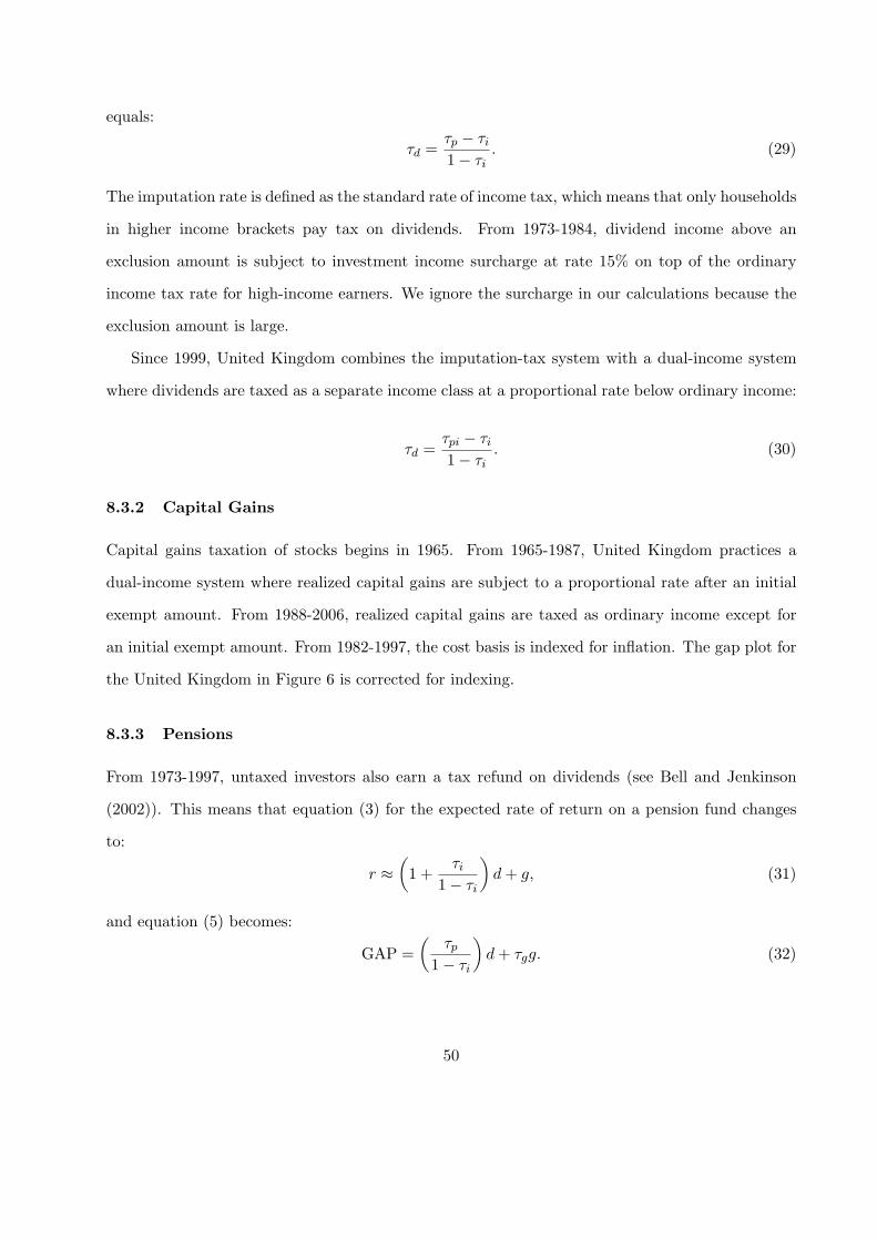
equals:

τd =τp − τi

1− τi. (29)

The imputation rate is defined as the standard rate of income tax, which means that only households

in higher income brackets pay tax on dividends. From 1973-1984, dividend income above an

exclusion amount is subject to investment income surcharge at rate 15% on top of the ordinary

income tax rate for high-income earners. We ignore the surcharge in our calculations because the

exclusion amount is large.

Since 1999, United Kingdom combines the imputation-tax system with a dual-income system

where dividends are taxed as a separate income class at a proportional rate below ordinary income:

τd =τpi − τi

1− τi. (30)

8.3.2 Capital Gains

Capital gains taxation of stocks begins in 1965. From 1965-1987, United Kingdom practices a

dual-income system where realized capital gains are subject to a proportional rate after an initial

exempt amount. From 1988-2006, realized capital gains are taxed as ordinary income except for

an initial exempt amount. From 1982-1997, the cost basis is indexed for inflation. The gap plot for

the United Kingdom in Figure 6 is corrected for indexing.

8.3.3 Pensions

From 1973-1997, untaxed investors also earn a tax refund on dividends (see Bell and Jenkinson

(2002)). This means that equation (3) for the expected rate of return on a pension fund changes

to:

r ≈(

1 +τi

1− τi

)d + g, (31)

and equation (5) becomes:

GAP =(

τp

1− τi

)d + τgg. (32)

50

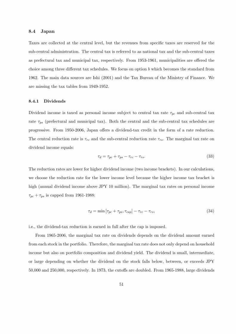
8.4 Japan

Taxes are collected at the central level, but the revenues from specific taxes are reserved for the

sub-central administration. The central tax is referred to as national tax and the sub-central taxes

as prefectural tax and municipal tax, respectively. From 1953-1961, municipalities are offered the

choice among three different tax schedules. We focus on option b which becomes the standard from

1962. The main data sources are Ishi (2001) and the Tax Bureau of the Ministry of Finance. We

are missing the tax tables from 1949-1952.

8.4.1 Dividends

Dividend income is taxed as personal income subject to central tax rate τpc and sub-central tax

rate τps (prefectural and municipal tax). Both the central and the sub-central tax schedules are

progressive. From 1950-2006, Japan offers a dividend-tax credit in the form of a rate reduction.

The central reduction rate is τrc and the sub-central reduction rate τrs. The marginal tax rate on

dividend income equals:

τd = τpc + τps − τrc − τrs. (33)

The reduction rates are lower for higher dividend income (two income brackets). In our calculations,

we choose the reduction rate for the lower income level because the higher income tax bracket is

high (annual dividend income above JPY 10 million). The marginal tax rates on personal income

τpc + τps is capped from 1961-1988:

τd = min [τpc + τps, τcap]− τrc − τrs, (34)

i.e., the dividend-tax reduction is earned in full after the cap is imposed.

From 1965-2006, the marginal tax rate on dividends depends on the dividend amount earned

from each stock in the portfolio. Therefore, the marginal tax rate does not only depend on household

income but also on portfolio composition and dividend yield. The dividend is small, intermediate,

or large depending on whether the dividend on the stock falls below, between, or exceeds JPY

50,000 and 250,000, respectively. In 1973, the cutoffs are doubled. From 1965-1988, large dividends

51

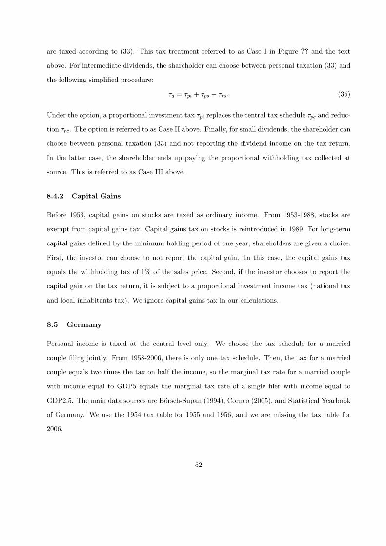
are taxed according to (33). This tax treatment referred to as Case I in Figure ?? and the text

above. For intermediate dividends, the shareholder can choose between personal taxation (33) and

the following simplified procedure:

τd = τpi + τps − τrs. (35)

Under the option, a proportional investment tax τpi replaces the central tax schedule τpc and reduc-

tion τrc. The option is referred to as Case II above. Finally, for small dividends, the shareholder can

choose between personal taxation (33) and not reporting the dividend income on the tax return.

In the latter case, the shareholder ends up paying the proportional withholding tax collected at

source. This is referred to as Case III above.

8.4.2 Capital Gains

Before 1953, capital gains on stocks are taxed as ordinary income. From 1953-1988, stocks are

exempt from capital gains tax. Capital gains tax on stocks is reintroduced in 1989. For long-term

capital gains defined by the minimum holding period of one year, shareholders are given a choice.

First, the investor can choose to not report the capital gain. In this case, the capital gains tax

equals the withholding tax of 1% of the sales price. Second, if the investor chooses to report the

capital gain on the tax return, it is subject to a proportional investment income tax (national tax

and local inhabitants tax). We ignore capital gains tax in our calculations.

8.5 Germany

Personal income is taxed at the central level only. We choose the tax schedule for a married

couple filing jointly. From 1958-2006, there is only one tax schedule. Then, the tax for a married

couple equals two times the tax on half the income, so the marginal tax rate for a married couple

with income equal to GDP5 equals the marginal tax rate of a single filer with income equal to

GDP2.5. The main data sources are Borsch-Supan (1994), Corneo (2005), and Statistical Yearbook

of Germany. We use the 1954 tax table for 1955 and 1956, and we are missing the tax table for

2006.

52

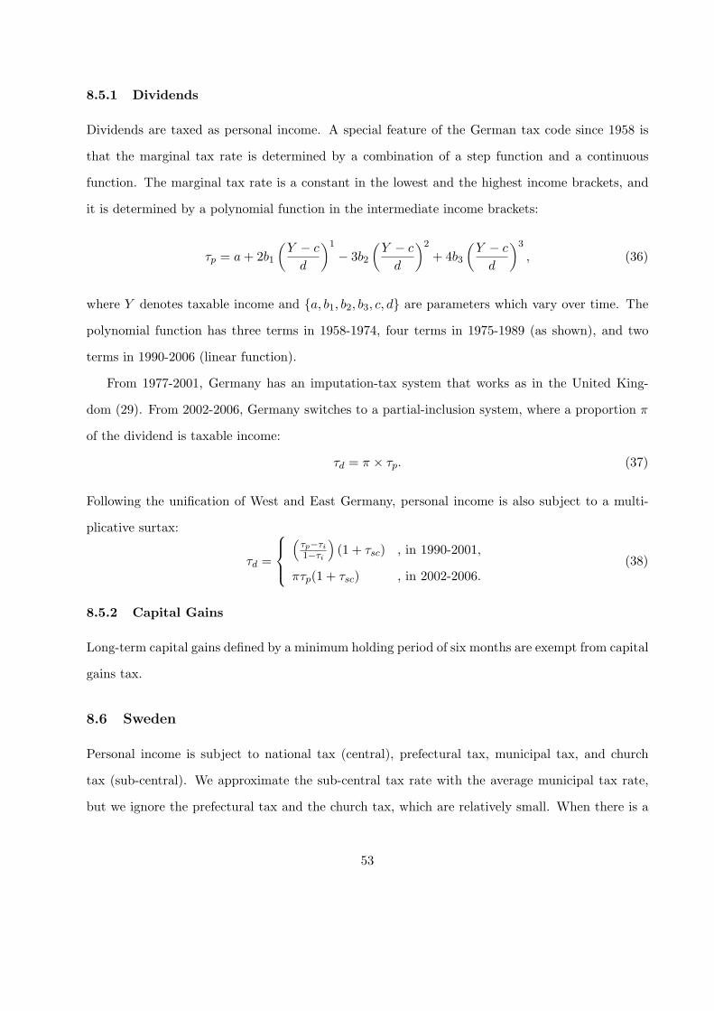
8.5.1 Dividends

Dividends are taxed as personal income. A special feature of the German tax code since 1958 is

that the marginal tax rate is determined by a combination of a step function and a continuous

function. The marginal tax rate is a constant in the lowest and the highest income brackets, and

it is determined by a polynomial function in the intermediate income brackets:

τp = a + 2b1

(Y − c

d

)1

− 3b2

(Y − c

d

)2

+ 4b3

(Y − c

d

)3

, (36)

where Y denotes taxable income and {a, b1, b2, b3, c, d} are parameters which vary over time. The

polynomial function has three terms in 1958-1974, four terms in 1975-1989 (as shown), and two

terms in 1990-2006 (linear function).

From 1977-2001, Germany has an imputation-tax system that works as in the United King-

dom (29). From 2002-2006, Germany switches to a partial-inclusion system, where a proportion π

of the dividend is taxable income:

τd = π × τp. (37)

Following the unification of West and East Germany, personal income is also subject to a multi-

plicative surtax:

τd =

(τp−τi

1−τi

)(1 + τsc) , in 1990-2001,

πτp(1 + τsc) , in 2002-2006.(38)

8.5.2 Capital Gains

Long-term capital gains defined by a minimum holding period of six months are exempt from capital

gains tax.

8.6 Sweden

Personal income is subject to national tax (central), prefectural tax, municipal tax, and church

tax (sub-central). We approximate the sub-central tax rate with the average municipal tax rate,

but we ignore the prefectural tax and the church tax, which are relatively small. When there is a

53

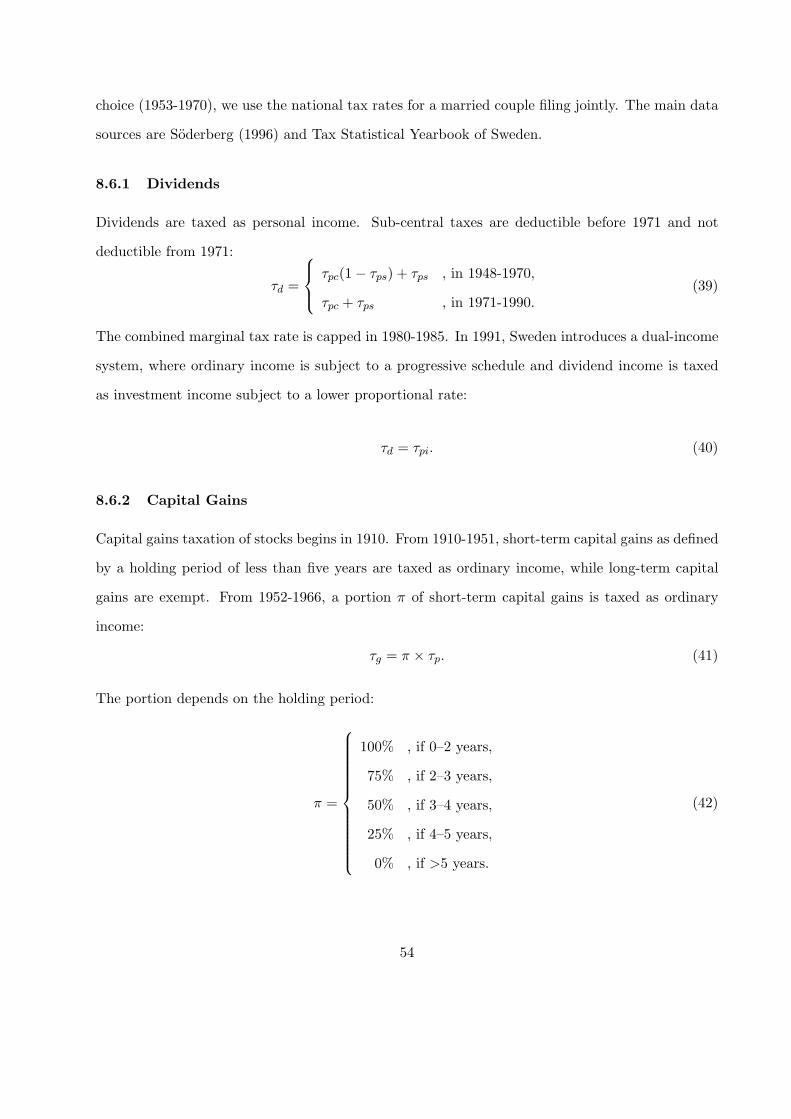
choice (1953-1970), we use the national tax rates for a married couple filing jointly. The main data

sources are Soderberg (1996) and Tax Statistical Yearbook of Sweden.

8.6.1 Dividends

Dividends are taxed as personal income. Sub-central taxes are deductible before 1971 and not

deductible from 1971:

τd =

τpc(1− τps) + τps , in 1948-1970,

τpc + τps , in 1971-1990.(39)

The combined marginal tax rate is capped in 1980-1985. In 1991, Sweden introduces a dual-income

system, where ordinary income is subject to a progressive schedule and dividend income is taxed

as investment income subject to a lower proportional rate:

τd = τpi. (40)

8.6.2 Capital Gains

Capital gains taxation of stocks begins in 1910. From 1910-1951, short-term capital gains as defined

by a holding period of less than five years are taxed as ordinary income, while long-term capital

gains are exempt. From 1952-1966, a portion π of short-term capital gains is taxed as ordinary

income:

τg = π × τp. (41)

The portion depends on the holding period:

π =

100% , if 0–2 years,

75% , if 2–3 years,

50% , if 3–4 years,

25% , if 4–5 years,

0% , if >5 years.

(42)

54

From 1967-1976, 10% of the sales price of a security held more than five years is taxed as ordinary

income. From 1977-1990, the formula for the inclusion proportion changes to:

π =

100% , if 0–2 years,

40% , if >2 years.(43)

From 1991-2006, all capital gains are taxed as investment income:

τg = τpi. (44)

The tax rule in effect 1967-1976 removes the basis from the calculation of the long-term capital

gain. As above, let g denote nominal stock price growth rate. The statutory marginal tax rate on

long-term capital gains equals:

τg = 10%τp

((1 + g)N

(1 + g)N − 1

). (45)

This expression shows that the effect on the marginal tax rate from the loss of the basis is small

over long investment horizons, especially when expected stock price growth is high. The value of

the basis protection disappears in the limit as N goes to infinity. In the analysis above, we assume

that N = 15, g = 2% + i, where i equals three-year moving average inflation.

8.6.3 Pensions

From 1991-2006, imputed income from pension asset management defined as the average treasury

rate during the previous year times the value of the pension assets in the beginning of the year is

taxed at the proportional rate 15%. We denote the expected treasury rate with rf and measure it

as 1% plus moving average inflation. Equation (5) becomes:

GAP = τdd + τgg − 15%rf . (46)

55

8.7 Finland

Income taxation in Finland resembles Sweden in many ways. Personal income is subject to national

tax (central), municipal tax, and church tax (sub-central). We approximate the sub-central tax

rate with the average municipal tax rate, but we ignore the relatively small church tax. We use the

national tax tables for a married couple filing jointly with no dependents (1950-1975). The main

data sources are Kukkonen (2000), the Finnish Tax Administration, and Statistics Finland.

8.7.1 Dividends

From 1950-1992, dividends are taxed as ordinary income. The marginal tax rate on dividends

equals the sum of central and sub-central tax rates:

τd = τpc + τps. (47)

From 1993-2004, Finland uses a dual-income system with full imputation. Dividends are subject

to investment income tax at rate τpi and corporate tax is credited back through imputation as in

the United Kingdom:

τd =τpi − τi

1− τi. (48)

Most years, the investment income rate equals the imputation rate so that τd = 0. Recently, in

2005-2006, Finland replaces the imputation system with a partial-inclusion system such that a

proportion π of the dividend is taxed as investment income:

τd = π × τpi. (49)

8.7.2 Capital Gains

Capital gains taxation of stocks begins in 1920. From 1920-1985, short-term capital gains as defined

by a holding period of less than five years are taxed as ordinary income, while long-term capital

gains are exempt. From 1986-1992, the rules change gradually towards the new system in place

since 1993. An initial (large) amount is tax exempt. A portion π of the capital gain above the

56

tax-exempt amount is taxed as ordinary income:

τg = π × τp. (50)

The portion depends on the holding period. From 1986-1988 it is:

π =

100% , if 0–5 years,

20% , if >5 years,(51)

from 1989-1990:

π =

100% , if 0–4 years,

80% , if 4–5 years,

40% , if >5 years,

(52)

and from 1991-1992:

π =

100% , if 0–4 years,

80% , if 4–5 years,

50% , if >5 years.

(53)

From 1993-2006, all capital gains on stocks are taxed as investment income:

τg = τpi. (54)

Since 1986, a long-term investor has the option to define the capital gain as 50% of the sales price

from 1986-1992 and 30% from 1993-2006. In our calculations, we ignore this option and the initial

tax-exempt amount because the difference is small.

57