Embed Size (px)
Citation preview

The Evolution of Cosmological DensityFluctuations
by
Bhuvnesh Jain
Submitted to the Department of Physicsin partial fulfillment of the requirements for the degree of
Doctor of Philosophy
at the
MASSACHUSETTS INSTITUTE OF TECHNOLOGY
May 1994
� Bhuvnesh Jain, MCMXCIV. All rights reserved.
The author hereby grants to MIT permission to reproduce anddistribute publicly paper and electronic copies of this thesis
document in whole or in part, and to grant others the right to do so.MASSACHtISOT.S INSMUre
-?��LoGy
MAY 2 1994
A uth or ... ...... ..... ............................. .......Department of Physics
May 13, 1994
Certified by. ........ .... .... / '? ............................Edmund Bertschinger
Associate ProfessorThesis Supervisor
Certified by .... ( . . . . . . . . . . . . . . . . . . . . . . . . . . . . . . .
Alan H. GuthProfessor
Thesis Supervisor
A ccepted by ........... ................. .....................George F. Koster
Chairman, Departmental Committee on Graduate Students

by
Bhuvnesh Jain
Submitted to the Department of Physicson May 13, 1994, in partial fulfillment of the
requirements for the degree ofDoctor of Pilosophy
AbstractWe study two distinct aspects of the evolution of cosmological fluctuations. The firstis the generation and evolution of quantum fluctuations in inflation with inducedgravity. The spectrum of density perturbations, SpIp, is estimated in the extendedinflationary model, in which the scalar curvature is coupled to a Brans-Dicke field.Through a conformal transformation and a redefinition of the Brans-Dicke field, theaction of the theory is cast into a form with no coupling to the scalar curvature anda canonical kinetic term for the redefined field. Following Kolb, Salopek and Turner,we calculate 8plp using the transformed action and the standard recipe developed forconventional inflation. The spectrum behaves as a positive power of the wavelength,a feature of relevance in building models to account for the observed large scalestructure of the universe.
The second part of the thesis deals with the nonlinear evolution of density per-turbations during the matter ominated era. In the weakly nonlinear regime we findthat the dominant nonlinear contribution for realistic cosmological spectra is madeby the coupling of long-wave modes and is well estimated by second order perturba-tion theory. For realistic spectra we find that due to the long-wave mode coupling,characteristic nonlinear masses are larger at higher redshifts than would be estimatedusing a inear extrapolation. For the cold dark matter model at (1 + z = 20, 10, 5 2)the nonlinear mass is about 180,8,2.5,1.6) times (respectively) larger than a linearextrapolation would indicate, if the condition rms 8pl = is used to define thenonlinear scale. At high redshift the Press-Schechter mass distribution significantlyunderestimates the abundance of high-mass objects for the cold dark matter model.Finally, we investigate possible long-wave divergences in the evolution of scale freespectra, pk) C n' using analytic techniques and N-body simulations. For n < -1,there are divergent terms in the evolution of the phases of the Fourier space den-sity field. We give a kinematical interpretation of this divergence and demonstratethat the self-similar scaling of physically relevant measures of perturbation growth ispreserved.
The Evolution of Cosmological Density Fluctuations

6
Thesis Supervisor: Edmund BertschingerTitle: Associate Professor
Thesis Supervisor: Alan H. GuthTitle: Professor

It has been a pleasure and a privilege to have the guidance of Ed Bertschinger and
Alan Guth for this thesis. The first part of the thesis was done in collaboration with
Alan, though my association with him continued through all my research work. The
extended, weekly meetings with him from my first months to the last have been one
of my most fruitful experiences at MIT. Alan has also been a friend and mentor in
every sense, and been unfailingly supportive through many difficult times. The major
portion of this thesis is a collaborative effort with Ed Bertschinger. Most of what
I have learned about research in large scale structure I owe to Ed. His energy and
versatility have been a source of inspiration, and his personal concern and enthusiastic
guidance of my work have been crucial at every stage.
I am grateful to Paul Schechter for useful comments on the thesis, persuasive
advice through the years and for his entertaining company in the Common Room.
My interest in theoretical physics and cosmology was initiated and shaped by Ra-
jendra Poph, ichard Gott, Jim Peebles, Bharat Ratra and David Weinberg, with
all of whom I have continued to have useful iscussions. It is a pleasure to thank
Simon White for his hospitality at the Institute of Astronomy and many stimulating
discussions.
This thesis owes a lot to many others - I would especially like to thank: Priya who
has made the years at MIT so special, for wonderful companionship and support at
every stage; my parents and Bena for their constant support and encouragement over
the years, in this and in every other venture I have undertaken; Shep Doeleman for
the magic of imbuing Building 6 with warmth and humor, and for many memorable
squash bruises; Chris Naylor for his help, concern and humor in handling all manner
of problems and Evening many a lunch hour; Mira, John Tsai and Ranga for their help
and advice in the difficult first years at MIT; Janna for lessons in creative cosmology
and timely reminders of life beyond Physics; Mark with whom I shared the long hours
of the final month's writing, for pleasant company and for solving all my computer-
related woes; Jim Frederic, Lam, Uros, Neal, John Blakeslee, Anand, Juliana, Chung-
Acknowledgments

Pei, Jim Gelb and Rosanne for entertaining company and unfailing support; Esko
for enjoyable times while sharing an apartment, coffee breaks and Finnish licorice;
Meenu for great company that livened many an evening, and for her thoughts on wave
propagation; Sonit for sharing the ups and downs of the past year; Arunjot, Sowmya,
Ranjan and Niranjan for their company and many culinary delights; and the Coffee
Shop and its workers for cheap supplies and consistently jarring music which left me
no choice but to get back to work.
This thesis is dedicated to my parents.

1Published in Phys. Rev. D 45, 426 1992)2To be published in Ap. J., 431 1994)
1 Introduction
1.1 Fluctuations in Inflation . . . . . . . . . . . . . . . . .
1.2 The Growth of Density Fluctuations . . . . . . . . . .
2 Density Fluctuations in Extended Inflation'
2.1 Introduction . . . . . . . . . . . . . . . . . . . . . . . .
2.2 Jordan Frame Results . . . . . . . . . . . . . . . . . .
2.3 Einstein Frame Results . . . . . . . . . . . . . . . . . .
2.4 Calculation of 6plp . . . . . . . . . . . . . . . . . . . .
2.5 Comments . . . . . . . . . . . . . . . . . . . . . . . . .
2.5.1 Comparison with the Naive Jordan Frame Result
2.5.2 Comparison with KST's Results . . . . . . . . .
2.5.3 Application to Generalized Gravity Theories
2.6 Conclusion . . . . . . . . . . . . . . . . . . . . . . . . .
9
9
12
16
16
18
19
22
26
26
27
28
30
. . . . . . .
. . . . . . .
. . . . . . .
. . . . . . .
. . . . . . .
. . . . . . .
. . . . . . .
. . . . . . .
. . . . . . .
. . . . . . .
. . . . . . .
3 Second Order Power Spectrum and Nonlinear Evolution
Redshift2
3.1 Introduction ...........................
3.2 Perturbation Theory . . . . . . . . . . . . . . . . . . . . . .
3.2.1 General Formalism . . . . . . . . . . . . . . . . . . .
3.2.2 Power Spectrum at Second Order . . . . . . . . . . .
at High
36
36
40
40
43
. . . . .
. . . . .
. . . . .
6
Contents

3.3 Results for CDM . . . . . . . . . . . . . . . .
3.3.1 Nonlinear Power Spectrum . . . . . .
3.3.2 Comparison with N-Body Simulations
3.3.3 Scaling in Time . . . . . . . . . . . . .
3.3.4 Distribution of Nonlinear Masses . . .
3.4 Discussion . . . . . . . . . . . . . . . . . . . .
. . . . . . . . . . . . 4 6
. . . . . . . . . . . . 4 6
. . . . . . . . . . . . 5 1
. . . . . . . . . . . . 5 3
. . . . . . . . . . . . 5 6
. . . . . . . . . . . . 58
4 Self-Similar Scaling of Density Fluctuations
4.1 Introduction . . . . . . . . . . . . . . . . . . . . . . . . . . . .
4.2 Long Wave Divergences for n < 1 . . . . . . . . . . . . . . .
4.3 Self-Similarity and Perturbation Theory . . . . . . . . . . . .
4.3.1 Formalism . . . . . . . . . . . . . . . . . . . . . . . . .
4.3.2 Long Wave Divergences in Perturbative Contributions
4.4 Analytic Approximation for Long Wave Mode Coupling . . . .
4.4.1 Solution for the Phase Shift . . . . . . . . . . . . . . .
4.4.2 Taylor Series Expansion . . . . . . . . . . . . . . . . .
4.5 Self-Similar Scaling in N-body Simulations . . . . . . . . . . .
4.6 Conclusion . . . . . . . . . . . . . . . . . . . . . . . . . . . . .
70
. . . 70
. . . 77
. . . 80
. . . 80
. . . 82
. . . 85
. . . 85
. . . 91
. . . 94
. . . 100
7

List of Figures
2-1 Correction Factor for Einstein Frame . . . . . . . . . . . . . . . . . . 35
3-1 Nonlinear Power Spectrum for CDM . . . . . . . . . . . . . . . . . . 65
3-2 Second Order Contributions to P(k) . . . . . . . . . . . . . . . . . . 66
3-3 Smoothed RMS Density Contrast . . . . . . . . . . . . . . . . . . . . 67
3-4 Characteristic Nonlinear Mass as a Function of Time . . . . . . . . . 68
3-5 Cumulative Mass Fraction at Different Mass Scales . . . . . . . . . . 69
4-1 "Raw" Phase Trajectories for n = 2 . . . . . . . . . . . . . . . . . . 104
4-2 "Re-defined" Phase Trajectories for n = 2 . . . . . . . . . . . . . . 105
4-3 Amphtude Trajectories for n -2 . . . . . . . . . . . . . . . . . . . 106
4-4 Mean Phase Deviation for n -2 . . . . . . . . . . . . . . . . . . . . 107
4-5 Mean Amplitude for n = 2 . . . . . . . . . . . . . . . . . . . . . . . 108
4-6 Characteristic Scales from the Phase for n = 2 . . . . . . . . . . . . 109
4-7 Characteristic Scales from the Amplitude for n = 2 . . . . . . . . . 110
4-8 Mean Phase Deviation for n = . . . . . . . . . . . . . . . . . . . . . 111
4-9 Mean Amplitude for n = . . . . . . . . . . . . . . . . . . . . . . . . 112
4-10 Characteristic Scales from the Phase for n = . . . . . . . . . . . . . 113
4-11 Characteristic Scales from the Amplitude for n = . . . . . . . . . . 114
8

Chapter I
Introduction
The first part of this thesis comprising Chapter 2 is a calculation of the density
perturbation spectrum produced in the extended inflationary model. This work was
done in collaboration with Alan Guth. The second part of the thesis comprising
Chapters 3 and 4 is a study of the nonlinear evolution of density perturbations during
the matter dominated era. This work was done in collaboration with Ed Bertschinger.
In this Chapter I shall provide a brief introduction to both parts of the thesis. For
details the reader is referred to the pedagogical review of inflation given by Blau
Guth 1987), and to Peebles 1980) for a review of theoretical approaches to large
scale structure.
1.1 Fluctuations in Inflation
Inflation is a hypothetical period of rapid expansion of the universe in its very early
history. It can arise quite naturally in Grand Unified Theories of particle physics
at very high temperatures when the energy density of the universe is dominated by
the potential energy density [V(O)] of a scalar field . If O) is constant, then
the expansion scale factor a(t) expands exponentially in time. This is known as de
Sitter spacetime, and it provides the arena for calculating the detailed evolution of
the inflationary universe.
One of the successes of inflationary cosmology is the generation of quantum fluc-
9

tuations which give rise to density fluctuations after the universe makes a transition
to the radiation dominated 7 and subsequently, the matter dominated era. The pre-
dicted spectrum of density fluctuations is the scale-invariant spectrum in which the
amplitude at horizon crossing is independent of scale. This spectrum has been popu-
lar in cosmology even before its origin was explained in the context of inflation. It is
in approximate agreement with observations of the distribution of galaxies (after the
spectrum at small scales is modified during the radiation dominated era), and with
the microwave background fluctuations detected by the COBE satellite. In Chapter
2 we present a calculation of the density fluctuation spectrum in a recently proposed
model of inflation known as extended inflation. This model is based on the Brans-
Dicke theory of gravity. In extended inflation the scale factor expands as a power
law in time, hence the background spacetime is no longer de Sitter. We find that
the resulting density perturbation spectrum has slightly more power on large scales
as compared to the scale-invariant spectrum. As a background to the calculation
presented in Chapter 2 the standard calculation of the density fluctuation spectrum
in inflation with de Sitter spacetime is qualitatively described here.
The goal of such a calculation is to compute the density perturbations in the
post-inflationary era induced by the quantum fluctuations in which are generated
during inflation on all scales within the event horizon. They rapidly cross outside the
horizon due to the exponential expansion of space. After inflation when the horizon
grows faster than the scale factor, these fluctuations enter the horizon as density
perturbations. The scale invariance of the spectrum of standard inflation is related to
the time-translation invariance of de Sitter spacetime: the physical size of the event
horizon and the expansion rate are constant in time. Therefore scales which cross
outside the horizon at different times do so under identical conditions, hence they
have equal amplitude. Once outside the horizon causal processes cannot alter their
growth, therefore when they enter the horizon after inflation they still have equal
amplitude. This simple expectation is borne out by detailed calculations which are
briefly outlined below.
The relevant wavelengths cross outside the horizon while the scalar field is still
10

very near the peak of the effective potential at = so during this period we can
take O) V(O = constant. The metric for the background de Sitter spacetime is
thend52 = _dt2 + a t ) 2 dX-42
with a(t) eHt , where H is a constant proportional to �Vw- With this metric
the classical equations of motion for -,t) can be obtained from its Lagrangian.
Next is written as 0:F, t = Oo(t) + 80(:F, t), where 60(x-, t) represents the quantum
fluctuations in . With this substitution the following equation of motion for 50(x- t)
is obtained:
+ 3H�o = e -2MV28 _ 92V (00) 60. (1.2),902
We proceed by observing that at very early times the term involving O) on the
right-hand side of equation 1.2) is negligible (since the first term on the right-hand
side is exponentially large), so that can be approximated as a free, massless scalar
field in de Sitter spacetime. For such a field the propagator is known, and can be used
to estimate the root mean square fluctuations in , denoted by AO. At late times on
the other hand, the first term on the right-hand side becomes negligible, so 80 obeys
the same equation as the homogeneous part Oo(t). One of the two solutions to this
differential equation is found to damp quickly, so the solution at large t is unique. In
terms of this solution, 80 can be written as 80(4 t) Oo(t) 8r(:F), and to first order
can be expressed as:
OP 0 0 W - �0 M 6T V) - 00 ( 6 M) (1.3)
Hence at late times the effect of the fluctuations is to cause a position dependent time
delay 8r(i) in the evolution of Oo(t).
Thus one obtains the following simple physical picture of the generation of fluc-
tuations. As X-, t) approaches a minimum of O), the energy density in the false
vacuum gets converted into matter and radiation and provides the exit from the infla-
tionary phase. The final expression in equation 1.3) indicates that different regions in
11

space follow the same history, but slightly offset in time due to the spatial dependence
of 5r(x-). Hence they exit the inflationary era at ifferent times - this causes their
temperatures at a given time early in the radiation dominated era to differ sghtly,
thus generating fluctuations in the post-inflationary epoch. These are calculated by
introducing a new time variable t' which is the argument of in the final expression
in equation 1.3). The perturbations are then recorded in the redefined metric which
has t' as its time variable. By introducing the energy momentum tensor of a perfect
fluid for the radiation dominated era the spectrum of the energy density perturba-
tions is obtained in terms of 8r. The latter is estimated by matching the early time
expression for AO with the late time approximation of equation 1.3). The result-
ing spectrum depends on H(oc VO)), and therefore the parameters of the particle
physics model, through AO. The result for the rms density contrast smoothed on a
given scale is 6pl - H 2/�' where the right-hand side is evaluated at the time that
scale crossed outside the event horizon during inflation.
1.2 The Growth of Density Fluctuations
If the scale invariant spectrum were to remain unmodified on entering inside the
horizon it would be of the form P(k) o k for all k. This spectrum is scale invariant
in the sense that the amplitude of the rms smoothed density contrast is independent
of scale at the time of horizon crossing. The relation of the power spectrum at a
given time to the spectrum of the rms 8plp smoothed on the comoving length scale
x at horizon crossing can be obtained by noting that WM, e-, a(t)x-1 for the scale
invariant spectrum. Now consider a mode that enters the horizon in the radiation
dominated era at time t when its physical wavelength A = a(t,,)x = t,. Since
a(t) OC t1/2 during the radiation dominated era, a(t,,) x x. Hence it follows that at
the time of horizon crossing, 6plp), - a(t,,) x-' is independent of the length scale x.
The physical processes operating within the horizon in the radiation dominated era
modify the spectrum at high k. Once a fluctuation scale enters the acoustic horizon
during the radiation dominated era, it is acted on by processes that arise due to the
12
coupling of baryons to photons. The baryon-photon fluid oscillates like an acoustic
wave due to radiation pressure, therefore fluctuations in this component cease to grow.
Perturbations in non-relativistic dark matter also remain almost constant until the
beginning of the matter dominated era due to the rapid expansion of the background.
In addition, there are possible damping processes such as the Silk damping of adiabatic
perturbations and neutrino free streaming which erase fluctuations on small scales.
Hence the spectrum at small scales gets frozen or damped, while on scales outside
the acoustic horizon it continues to grow.
Once the universe becomes matter dominated and recombination occurs, pertur-
bations in the matter density grow as they are no longer coupled to photons and are
Jeans unstable. The scales which enter the horizon during this epoch have remained
virtually unaffected by the radiation dominated era. This causes the spectrum to
retain the shape P(k) o k on these large scales, while it approaches the asymp-
totic form P(k) o k-' on very small scales. The k-3 spectrum on small scales
corresponds to density perturbations 6p1p).,,, which have equal amplitude as a func-
tion of scale at a given time. The scale that provides the transition between these
asymptotic features is, to within an order of magnitude, the size of the horizon at
matter-radiation equality, about 10(Qh 2)-l Mpc for a Cold Dark Matter dominated
universe (1 Mpc 3 x 1021 cm; h is the value of the Hubble parameter today in units
of 100 km/s/Mpc). The detailed shape of the resulting post-recombination spectrum
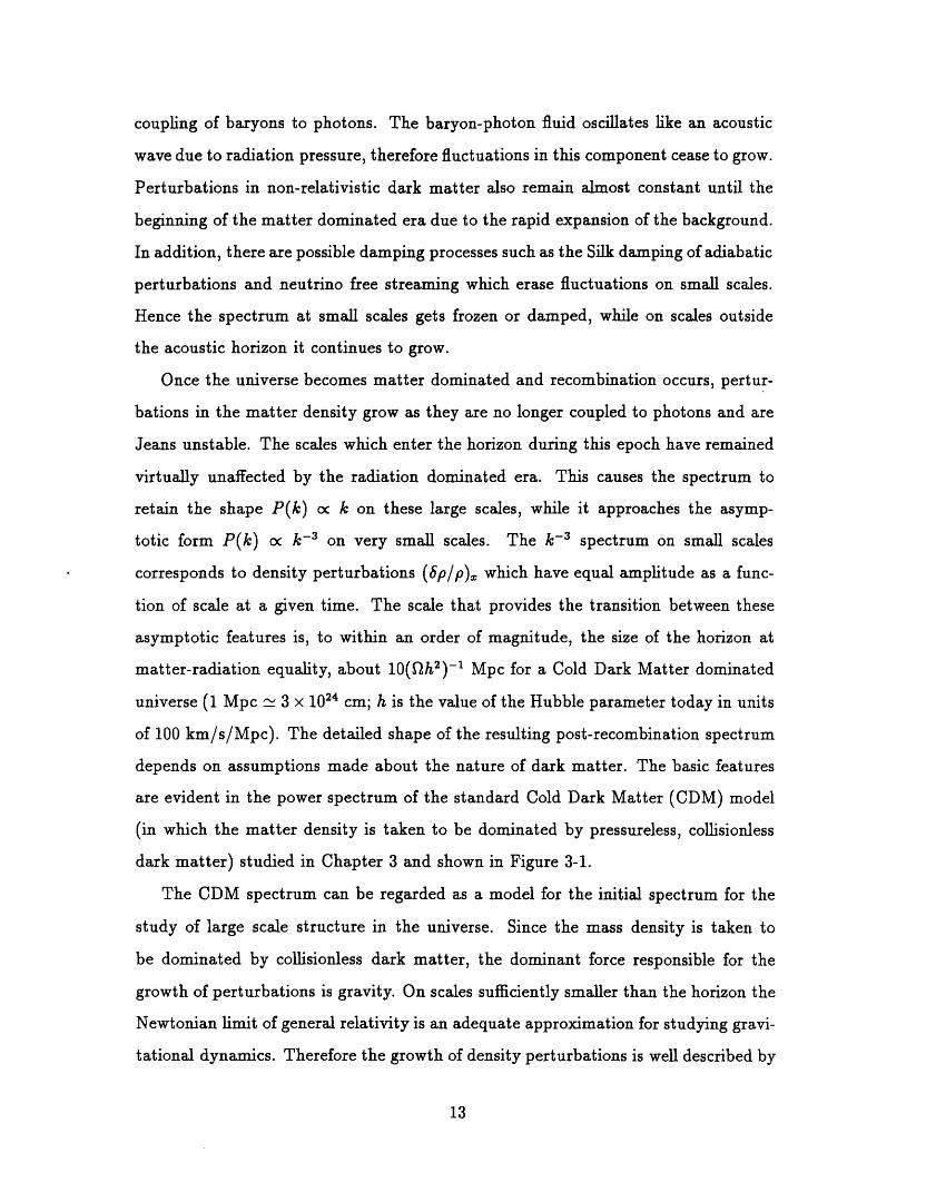
depends on assumptions made about the nature of dark matter. The basic features
are evident in the power spectrum of the standard Cold Dark Matter (CDM) model
(in which the matter density is taken to be dominated by pressureless, collisionless
dark matter) studied in Chapter 3 and shown in Figure 31.
The CDM spectrum can be regarded as a model for the initial spectrum for the
study of large scale structure in the universe. Since the mass density is taken to
be dominated by collisionless dark matter, the dominant force responsible for the
growth of perturbations is gravity. On scales sufficiently smaller than the horizon the
Newtonian Emit of general relativity is an adequate approximation for studying gravi-
tational dynamics. Therefore the growth of density perturbations is well described by
13

Newtonian fluid equations in the expanding coordinates appropriate for cosmology.
At the time of recombination (redshift z 1400) the -fluctuation amplitude on
scales of interest to large scale structure (about 1-100 Mpc) is very small. Therefore
at early times the growth of perturbations is accurately described by the linearized
cosmological fluid equations which show that the fractional density contrast grows as
5plp oc a(t). When the perturbation amplitude grows to be of order unity, nonlinear
effects become significant and cause the perturbation to cease expanding and then to
collapse. Such collapsed structures become the sites for the formation of galaides a
process in which dissipative processes play an important role as well. Cosmological
spectra Eke the CDM spectrum have increasing amounts of power on smaller length
scales. Therefore the first scales to collapse are likely to be the smallest, and there-
after structure formation proceeds hierarchically on larger scales. This picture is a
simplified version of the standard lore in large scale structure studies. It provides the
context in which the work presented in Chapters 3 and 4 can be placed.
14

Blau, S.K. & Guth, A.H. 1987, in 300 Years of Gravitation, eds. Hawking, S.W.
Israel, W. (Cambridge: Cambridge University Press)
Peebles, P. J. E. 1980, The Large-Scale Structure of the Universe, (Princeton: Prince-
ton University Press)
15
REFERENCES

Chapter 2
Density Fluctuations in Extended
Inflationi
2.1 Introduction
Extended inflation is a new model of inflation, proposed by La and Steinhardt [1]. Its
key feature is that the effective gravitational constant G varies with time due to the
non-minimal coupling of a scalar field to the scalar curvature R. As first proposed
[1], it was based on the Brans-Dicke 2] theory of gravity, for which the action is given
by 3]S d4xr- R gAV8;"4o'-q�
g - ) + - + matte (2.1)167r 167r 1(b
Withl =_ 27rO2/W' the kinetic term for the scalar field can be written in the standard
way:S d4x,/-- R 1
g _ 02 -9 AV apoaVo +Cmatter (2.2)8w 2
We shall work with 2.1), the form originally introduced by Brans and Dicke.
The Brans-Dicke field 4P couples to gravity and is responsible for the time variation
of G. The inflaton field a contributes t Cm.tter and provides the nearly constant
vacuum energy density that drives inflation. is a dimensionless parameter of the
IPublished in Phys. Rev. D 45, 426 1992)
16

theory: Brans-Dicke gravity becomes identical to Einstein gravity as approaches
infinity.
In contrast to the exponential expansion of standard inflation, the time variation
of G in extended inflation leads to a power law expansion of the scale factor at).
The Hubble parameter H =_ oi/a is therefore decreasing with time. Once H becomes
sufficiently small, the transition to a radiation-dominated universe can be completed
by bubble nucleation, providing the possibility of a graceful exit to the false vacuum
phase. If H changes too slowly, however, then the problems of the original infla-
tionary scenario remain- a nearly scale-invariant distribution of bubbles is formed,
resulting in large inhomogeneities and distortions of the cosmic background radiation.
These distortions are unacceptably large unless 25 4], whereas time-delay ex-
periments constrain to be 2. 0 6 This problem can be avoided by introducing
potential for the field which has a minimum at = G-1, where GN i the present
value of the gravitational constant. Thus, a scalar field that couples to gravity can
be used to construct an interesting cosmological model. The physics of this coupling
is interesting in any case, because a number of particle theories-superstring, super-
gravity, and Kaluza-Klein theories, for example-involve such a coupling. In general,
terms with higher order couplings of to the scalar curvature are also possible.
Steinhardt and Accetta 7] have studied a generalization of extended inflation, called
hyperextended inflation, in which the consequences of such higher order coupling
terms are explored.
In this paper we compute the density perturbation spectrum 5plp in the context
of La and Steinhardt's original model of extended inflation. Specifically, we compute
the curvature fluctuations that arise from quantum fluctuations in the 4� field. We
work with the simple Brans-Dicke action because it provides tractable equations of
motion.
We begin in Section 22 by obtaining the equations of motion in the Jordan frame,
i.e., the frame defined by the action 2.1). In Section 23, following Holman et al. [8],
we make a conformal transformation that takes the action to the standard Einstein-
Hilbert form. In this conformally rescaled frame, known as the Einstein frame, a
17
rescaled time variable is introduced and the equations of motion axe derived. A
new field IQ, obeying the equations of motion of a minimally coupled scalar field, is
defined in terms of 4�. As pointed out by Kolb, Salopek and Turner 9 (hereafter
called KST), this form of the action allows us to directly apply the results for SpIp
obtained in standard inflation 10-13]. The calculation of SpIp is carried out in
Section2.4. We point out some subtleties in the application of the standard density
perturbation results, but we leave the investigation of these subtleties to a future
paper. We nonetheless argue that the present result should be acceptable as an order-
of-magnitude estimate. In Section 25 our result is compared with that obtained by
naively applying the standard formalism in the Jordan frame. A calculation similar to
ours is carried out in KST, but our result differs from theirs by a factor that depends
on w. This discrepancy vanishes in the limit of large w, a limit in which both results
agree with the answer that would be obtained naively in the Jordan frame. We point
out what we believe are the reasons for the discrepancy. We also demonstrate that
the action for a more general class of gravity theories can in principle be transformed
to the form for a minimally coupled scalar field with a canonical kinetic term. We
summarize in Section 26.
2.2 Jordan Frame Results
In this section we summarize the homogeneous background solutions for 4t) and
the scale factor a(t) for the Jordan frame action 2. 1), assuming a flat (i. e., k = )
Robertson-Walker metric. We follow the notation of KST to facilitate comparison of
results.
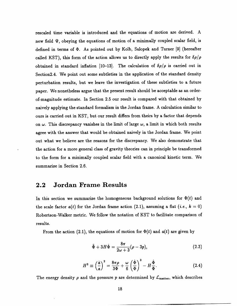
From the action 2.1), the equations of motion for 4t) and a(t) are given by
+ 3H,$ 87r (p - 3p), (2.3)2w 3
2 W 2a 87rpH2 - = - + - - H_ (2.4)
a 34) 6 4� 1P,
The energy density p and the pressure p are determined by Lm.tt,,, which describes
18

the inflaton field and all other matter fields:
lCmatter : 19'wO,,o,,Oo, - V(O, + (2.5)2
In extended inflation V(o,) provides the nearly constant false vacuum energy density
that dominates the energy density of the universe during inflation. Since the O' field
stays anchored very near its false-vacuum value, its kinetic energy is negligible. Thus
during inflation we have p - pv,,,,: and p - -pv,,,r., where Pv,,,c M' is the value of
V(o,) in the false vacuum. The desired solution can then be written
-1)(t = Do(Bt)2, (2-6)
a(t = ao(Bt)-+i, (2.7)+
2H(t = t (2.8)
whereM2
B 0 - I and q (2.9)qw
(Readers comparing with KST will note that we have chosen a different origin for the
time variable t.) Unlike exponential inflation I the Hubble parameter H in this case
is time-dependent.
2.3 Einstein Frame Results
In this section we make the conformal transformation [8] that defines the Einstein
frame in terms of the Jordan frame described above. The Einstein frame quantities
will be indicated by an overbar.
Define a new metric �,, as
gi. :F, t) 2 t_qA. t),XI (2.10)
wheref22(t) M21 (2.11)
'qqt)
19

and mp = G112 i the present value of the Planck mass. Define a field IQ in termsN
of by
IQ To In (2.12)
where
To _+3 M (2.13)PI
The field is introduced so that the kinetic term also takes the canonical form.
Carrying out the conformal transformation 2.10) (see, e.g., Birrel and Davies 14] for
the transformation of R[g,,,]) yields
4XVf-3 d + _§1'11(9"Ti9'T167rGN 2
1 T/To 21k/To M4+ -e- j1"Aaco - e- (2.14)2
where we have used V(o-) = M4 . Notice that the gravitational part of has the
usual Einstein form, and that the kinetic term for also takes the canonical form.
Since the kinetic energy of the o- field is negligible, takes the form of the action for
a minimally coupled scalar field with an exponential potential,
v(T) =: m4 e-2'k/*o. (2.15)
In S, IF plays the role of the inflaton field-this identification simplifies the calculation
of /P [15].
We write the equations of motion in terms of a rescaled time variable so that
the metric takes the Robertson-Walker form
V = df _ df)2 dj = Q-2 (t) dS 2 (2.16)
where
d = Q -' dt) (2.17)
20

;1( = -la(t),
di = dx .
(2.18)
(2.19)
In these coordinates the equations of motion are
dV41(i) + 3.91�(O + = 0,
dT(2.20)
87r
3M2I(2.21)
In 2.20) and 2.21) and in all subsequent equations, an overdot indicates a derivative
with respect to E.
Using Eqs. 2.11) and 2.15), one sees that the desired conformal transformation
is given by
Q(t = MP,B (I)1/2t '0
(2.22)
The relation between and t can then be found by integrating Eq. 2.17), yielding
C = (Bt)2, (2.23)
with
C = 2Bmpi(pl/2
0
(2.24)
By combining Eqs. 2.6), 2.12), and 2.13), the Jordan frame solution for 4�(t) can
be transformed to give
T(f =
Eqs. 218), 222), and 223) lead to
d(o::
where
To In C(DofM21 (2.25)
2w+3= do(co (2.26)
(2.27)-11do = ao
The time-dependence of the Hubble parameter can be obtained by differentiating
21
2f12 = 40- W) 1,�2(1 + V(T)
2

Eq. 2.26), yielding2 3 (2.28)
4i
It is straightforward to verify that the equations of motion 220) and 221) are
satisfied by these transformed solutions.
2.4 Calculation of 6p1p
The equation of motion 2.20) for is the same as that for a minimally coupled
scalar field in standard inflation. This identification 9, 16] allows us to use the results
[10-13] for density perturbations arising from quantum fluctuations of a minimally
coupled scalar field. The ensity perturbation amplitude for a scale coming inside
the Hubble length in the late universe is then given by
6P fl(02(2.29)
P Hubbl. t=t,
where the right-hand side is to be evaluated at the time [h when the scale crossed
outside the Hubble length during inflation.
While the conformal transformation has eliminated the coupling between the
scalar field and gravity, we must still ask whether Eq. 229) is adequate for our
problem. There are several issues that must be considered:
(i) Even in the original context of standard inflation, the formula is only an ap-
proximation. It can be obtained, as in Ref. [11], by matching together an approximate
solution valid at early times and an approximate solution valid at late times. The
matching is done at the time of Hubble length crossing, a time when neither solution
is highly reliable. Alternatively, as in Ref. [10], it can be obtained by fixing the am-
plitude of the late time solution by using a rough estimate of quantum fluctuations at
early times. The approximation is good enough for most purposes, but here we face
the problem that the effects we will be studying are quite small- see, for example,
Fig. 1-1 below. To properly justify the consideration of such small effects, one wants
to know that the other uncertainties are even smaller. A rough estimate of the uncer-
22

tainty in formula 2.29) can be obtained by recognizing that the precise time at which
the right-hand side is to be evaluated has not been carefully thought out. While the
standard convention holds that it should be evaluated at Aphysical H-1, one might
just as well have decided to evaluate it when Aphysical 2H-1. This modification of
the rules, however, would produce an w-dependent correction that is comparable to
the size of the effects that will be considered below.
(ii) The standard derivations of Eq. 2.29) assumed that the �V term of the equation
of motion for is negligible, while we will find that this is not the case when is
small. Again there is no problem if Eq. 2.29) is considered an approximation, but
the accuracy that we desire will merit a more careful look at this approximation.
(iii) Eq. 2.29) was derived originally for exponential inflation, while here we are
applying it to power-law inflation, with a(t) oc P. The application to power-law in-
flation has been investigated by Lucchin and Matarrese 17], who conclude that the
standard formula is correct. This conclusion, however, is valid only as an approxima-
tion. Abbott and Wise [18] have shown, for example, that the two-point function that
is used to calculate the scalar field quantum fluctuations depends on the exponent p
in a complicated way. Moreover, if H depends on time, any answer that depends on
H must specify precisely the time at which it should be evaluated.
These issues, however, are separate from the question of evaluating the right-hand
side of Eq. 229). In this paper we will carry out this evaluation, postponing the
investigation of the subtle issues. We believe that the answer obtained below is a valid
order-of-magnitude estimate (similar in its accuracy to the standard results 10-13]
in conventional inflation), but it is not a precise calculation.
Since the equation of motion is obtained from the Einstein action with as the
time variable, we must be careful to evaluate the right-hand side of Eq. 2.29) by using
f and the Einstein frame Hubble parameter R(O. In order to express 8P/P)Hubbl,
as a function of a present-day length scale, we use the ratio of the scale factors at
the time of Hubble length crossing and the present time. In doing so we assume
that the transition from inflation to radiation domination occurs instantaneously at
a temperature T -_ M, and that the field 4�(t) does not vary significantly after the
23

end of inflation. Therefore we approximate
MPII (2.30)dN
where t, denotes the time at the end of inflation. We assume that Eq. 2.30) holds also
for all t 4. Then f22(t = M2 /J�(t) pt� for a t - t, so after the end of inflation thepi r-4
Einstein and Jordan frames coincide. The evolution of the perturbation amplitude
after inflation is therefore the same in both frames. We will need an expression for t-,
(the rescaled time variable at the end of inflation), which can be found by combining
Eqs. 26) and 2.23) to obtain 4�(f,, = C§of,, m2j. Then using Eqs. 2.24) and
(2.27), one hasf = qwmpi (2.31)
2M2
To evaluate 2.29) we use 2.28) for R(O and 2.25) for T(O to obtain
8P f12(f ) (2w 32 (2.32)
x�(O 16TofhP Hubbl.
To solve for fh, the rescaled time variable at the moment of Hubble length crossing,
we use
Aphysicaa(fh = i(fh)A, = I(fh)-' (2-33)
where AC denotes the comoving wavelength. This can be rewritten as
AC= Hffh)- (2.34)
where we have set the present value of the scale factor d(fo = 1. Since d(O oc T-1,
d(f.)/d(fo) ToIM, where To -- 29 K is the present photon temperature. Also,
h/f.)(2w+3)/4 from 2.26). We substitute these relations into 2.34 to
get2.+3
fh TO -4fhA (2.35)
t" M 2w+3
24

Solving for 1h and substituting in 2.32) we obtain
(2.36)
We now eminate To and by using Eqs. 2.13) and 2.31), obtaining SpIp in terms
of known quantities:
8W+r' 2w+3
P:� V27r 2W+ 2(2,,=I) 1 2w-1
2 ) qw2(2w+l)
( M 2w-1X 2w-1 .
MPI (A. TO) (2.37)
Since we set WO = 1, A,: is the physical wavelength at the present time. Remem-
bering that we are using units for which = c = k = one has the conversion
AcTo = Amp, x 1 Mpc x 29 K = 364 x 1021 Amp,,. Thus,
2.+36P I- - 2(, 3 1 2w-1
- %f27r 2 qwP bble
2(2.+I)M 2w-1 4
XI MPI (3.64 x 1025AMPC ) 2w-1 (2.38)
where q is defined in Eq. 29). This is our main result. Notice that beyond using
SpIp - f2(0/,�(I)' the only approximation that we have made is to neglect the
evolution of P(t) after the end of inflation.
4/(2W-1)In agreement with KST, we find that the perturbations are proportional to A
This means that extended inflation might be an attractive way to account for the as-
tronomical observations that show evidence for increased power on large scales.
25
)2 4(2 3 2c, 3 To AC 2w-1
16'Po jW2w+3
I 2w-1X =
te
8P
P bble
8P
P ble

2.5.1 Comparison with the Naive Jordan Frame Result
To see the effect on this calculation of the transformation to the Einstein frame 7 it is
interesting to compare our result 2.38) with the answer that would be obtained by
naively applying the standard formalism in the Jordan frame. Using an asterisk to
denote the naive calculation, we have
Sp H 2(t)(2.39)
P dO(t)ldt =tz
where is the field defined canonically by the action 2.2), and t* is the time ofh
Hubble length crossing as seen in the Jordan frame. In the following we denote the
time of Hubble length crossing as seen in the Einstein frame by t = th (and = fh for
the rescaled time variable), while the time of Hubble length crossing in the Jordan
frame is denoted by t = t* and = h). Our result for 6P/P)Hubble differs from the
naive result for two reasons:
(i) At a given time the quantities H2 1(doldt) and ft 2/(dT/df) are not equal.
Using the formulas from Section 22, one esily finds that
2 (t) 1)2H - v"27rw(2w + q (2.40)do(t)ldt 4M2t2
For comparison, the right-hand side of Eq. 2.32) can be expressed in terms of t by
using Eq. 2.23). One then finds
f12 VF2 _ 2w 3 2 H 2 (t)
d'P(Oldf 3 w + 1 dO(t)ldt (2.41)
(ii) The time of Hubble length crossing itself is different in the two frames. In the
Jordan frame this time is evaluated using
a(t')Ar =: H(t*)-' (2.42)
26
2.5 Comments

which is not equivalent to the Einstein frame relation 233). Using Eq. 223 to
evaluate th in terms of ih, one finds the relation
41 2u 3 2w-1- = (2.43)
t2 2w + 1 t*2h h
To put together the two sources of discrepancy, note that the correct expression
for 6P/P)Hubble i obtained by evaluating the left-hand side of Eq. 2.41) at [h, which
implies that the right-hand side is evaluated at th. According to Eq. 240) this
expression is proportional to 1/t2' which can be replaced by the right-hand side ofh
Eq. 2.43). The factors occurring in Eqs. 2.41) and 2.43) are then multiplied to give
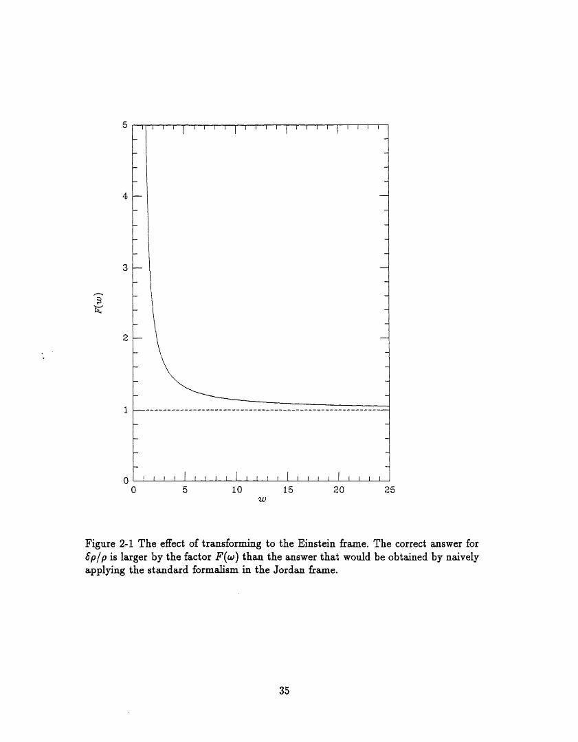
8P = F(w) 8 * (2.44)P ble P ubble
where the correction factor is given by
2(2w+l)F( 2w 2w 3 2.-1 (2.45)W =
w 3 2w + 1
The correction factor F(w) is plotted in Fig. 1-1. It decreases monotonically with ,
approaching one as approaches infinity.
We emphasize again that in the Einstein frame the field IF behaves as a minimally
coupled scalar field, and the rescaled time variable and scale factor d(O correspond
to a Robertson-Walker metric- therefore these functions not the original ones, must
be used in applying the standard methods to calculate (5PIP) Hubbl.-
2.5.2 Comparison with KST's Results
KST (Ref 9 have also worked with the Einstein frame action, but nonetheless their
answer (Eq. 221) of their paper) differs from ours: it is equal to our answer (Eq. 238)
times the factorF�6w+ �5 2w 2w-1 (2.46)
V 3(2 3 2 3)
This discrepancy is due to the following reasons:
27

(i) They evaluate F2 at the time of Hubble length crossing in the Jordan
frame, while we maintain that the time of Hubble length crossing must be evaluated
in the Einstein frame. According to Eq. 2.43), this causes their result to contain an
additional factor [(2w + 11(2w + 3)]4/(2,,,-1).
(ii) They use a "slow-rollover" pproximation -(dV/dT)/3fI(f), while we
evaluate 1�(f) by differentiating the exact solution for qf). This causes their result
to contain the additional factor 1�.Xactp�approx =3(2w + 31(6w + 5).
(iii) They evaluate 11 by using fl 2-- 8rV/3m21 (neglecting the kinetic energy),
while we used the exact expression. This causes their result to contain an additional
factor W-Pprox/kexact) 3 = (6w + 5) / 3(2w 3 3/2.
(iv) They omit a factor 2l(2w + 1) that should appear on the top line of their
Eq. 2.9). This causes their result to contain an additional factor [2wl(2w+ j)]4/(2--1).
Each of these discrepancy factors approaches one as approaches infinity, but in
this limit the effect of transforming to the Einstein frame disappears altogether.
The discrepancy factor 2.46) carries over into the formula for the temperature
fluctuations of the cosmic background radiation, (STIT)o>1o _ f2(f) /151�ff), given
as Eq. 2.25) in KST. For the same reasons, we would differ with KST's results for
graviton perturbations, Eqs. 2.13) and 2.16) in their paper. For the dimensionless
amplitude of a gravitational-wave perturbation as it comes inside the Hubble length
in the late universe, we obtain
2(2w+l) 2w+3M 2W-1 2w 3 2w-1
hx =MPI MPI 2q(.o
x 3-64 x 1025A.p,:) 2&a-1 (2.47)
2.5.3 Application to Generalized Gravity Theories
We have obtained the density perturbation spectrum for a simple model of extended
inflation. The method we have used, however, is applicable to a wide class of gener-
alized gravity theories that involve a scalar field coupled to gravity. Suppose that the
28
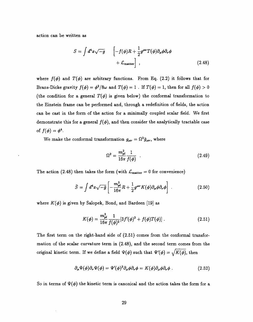
action can be written as
4.,/-- 1S d -f (O)R + 9 JAM T(0)(9,00MO2
+ lCmatte (2.48)
where f (0) and T(O) are arbitrary functions. From Eq. 22) it follows that for
Brans-Dicke gravity f (0) = 2 18w and T(O = 1 . If T(O = 1, then for a f (0 >
(the condition for a general T(O) is given below) the conformal transformation to
the Einstein frame can be performed and, through a redefinition of fields, the action
can be cast in the form of the action for a minimally coupled scalar field. We first
demonstrate this for a general f (0), and then consider the analytically tractable case
of f(o = 4.
We make the conformal transformation gA, = Q2�P" where
M 2pi (2.49)
16-7rf
The action 2.48) then takes the form (with .tt,, = for convenience)
4d m21 R + g" K (0) a,, OaM (2.50)16,7r 2
where K(O) is given by Salopek, Bond, and Bardeen 19 as
2
K (0 = mp' [3fl (0)2 + f (O)T(O)] (2.51)167rf(0)2
The first term on the right-hand side of 2.51) comes from the conformal transfor-
mation of the scalar curvature term in 2.48), and the second term comes from the
original kinetic term. If we define a field T(O) such that T'(0) =V K _(O) 7 then
,9AT(O),9MT(O = p0)2C9j'0,9MO = K(O),9AO,9�,O . (2.52)
So in terms of T(O) the kinetic term is canonical and the action takes the form for a
29

minimally coupled scalar field. For K(O > the integral
IFW = I VK�(O)�do (2.53)
is well defined and is a monotonically increasing function of , so there is a unique
value of T(O) (up to an additive constant) for every value of 0. Therefore one expects
that the quantum theory for gives the standard result, Eq. 2.29), for the density
perturbation spectrum. In general the integral for O) and the solutions of the
equations of motions must be obtained numerically.
For Brans-Dicke gravity, the integral for T(O) is simple and the result is given by
(2.12). TO) can also be obtained in closed form for the case f (0 = 4, T (0 = .
From Eq. 2.51) one has
- mp2l 4802 K(O = - 04 (2.54)167r
which can be integrated according to Eq. (2.53) to give
3mP1 /4802
IF 0) 7r 4802
02 )+ 1 n ( �,448 + 4 W (2-55)
In hyperextended inflation a term of this form may dominate the f (O)R coupling
during a cosmologically important epoch, so it is of some interest to study its density
perturbation spectrum [91.
A non-minimally coupled scalar field with f (0) = _ 2 has been studied by
Futamase and Maeda 20], who have obtained O) for a > .
2.6 Conclusion
We have estimated the density perturbation spectrum in the original model of ex-
tended inflation, with Brans-Dicke gravity. Curvature fluctuations arising from quan-
30

tum fluctuations in the Brans-Dicke field contribute a significant amplitude of density
perturbations. They are a slowly increasing function of the scale, a feature that might
be useful in building models to account for the observed large scale structure of the
universe. We have performed the calculation by transforming to the Einstein confor-
mal frame, then applying the standard procedures used in conventional inflationary
models. We have pointed out some subtleties associated with this procedure, but we
nonetheless believe that the result is valid as an order-of-magnitude estimate
We have compared our density perturbation amplitude to the answer that would
be obtained by working naively in the Jordan frame our answer is larger by a factor
that is near unity, but which becomes large for very small values of the Brans-Dicke
parameter w. If the calculation is done correctly in both frames, however, one should
of course expect to obtain the same answer. Indeed, part of our motivation was to
lay some groundwork toward a consistent calculation in the two frames. The success
of such a calculation would give us confidence that the field theory is being treated
correctly, and that the conformal transformation method is valid at the quantum (or
at least semiclassical) level as well as the classical level. The question of consistency
between the two frames has been addressed in two recent preprints 21].
As pointed out earlier, the model we have studied must be modified if it is to
satisfy experimental constraints. One possibility is to add a small mass term for the
Brans-Dicke field- the evolution of during the inflationary period would not be
significantly affected, but the mass term could still freeze the value of the field in the
present epoch so that the theory would be consistent with observation. As pointed out
by KST, in this scenario the 4� particles would have to be unstable in order to prevent
the mass density of the universe from becoming dominated by them. If the model is
repaired in this fashion, then the calculation of density fluctuations presented in this
paper would remain valid. One can also imagine more substantial modifications to
the model, in which case our calculation would no longer be valid in detail. It would
nonetheless serve as an illustration of a technique to compute 5P/P)Hubble for models
with a scalar field coupled to gravity.
31
The authors would like to thank Dalia Goldwirth and Tsvi Piran for interesting
discussions. They are also extremely grateful to Robert Brandenberger for many
valuable conversations.
The work of A.H.G. was supported in part by the U.S. Department of Energy
(D.O.E.) under contract #DE-AC02-76ER03069, and the work of B.J. was supported
in part by funds provided by the Karl Taylor Compton Fellowship.
32

REFERENCES
1 D. La and P. J. Steinhardt, Phys. Rev. Lett. 62, 376 (1989). An early paper de-
scribing some aspects of inflation in a Brans-Dicke theory is C. Mathiazhagan
and V. B. Johri, Class. Quantum rav. 1, L29 1984).
2 C. Brans and R. H. Dicke, Phys. Rev. 24, 925 1961).
3 See, for example, S. Weinberg, Gravitation and Cosmology (Wiley, New York,
1972).
4 D. La, P. J. Steinhardt, and E. Bertschinger, Phys. Lett. 231B, 231 1989).
' E. J. Weinberg, Phys. Rev. D40, 3950 1989).
' R. D. Reasenberg et al., Ap. J. 234, L219 1979).
7 . J. Steinhardt and F. S. Accetta, Phys. Rev. Lett. 64, 2740 1990).
8 R. Holman, E. W. Kolb, S. L. Vadas, Y. Wang, and E. J. Weinberg, Phys. Lett.
237B) 37 1990).
E. W. Kolb, D. S. Salopek, and M. S. Turner, Phys. Rev. D42, 3925 (1990).
'O J. M. Bardeen, P. J. Steinhardt, and M. S. Turner, Phys. Rev. D28, 679 (1983).
" A. H. Guth and S.-Y. Pi, Phys. Rev. Lett. 49, 1100 1982).
12 A. A. Starobinski, Phys. Lett. 117B, 175 1982).
13 S. W. Hawking, Phys. Lett. 115B, 295 1982).
N. D. Birrell and P.C.W. Davies, Quantum Fields in Curved Space (Cambridge
University Press, Cambridge, England, 1982).
In the Jordan frame the effective gravitational constant Gff = V1 is time-
dependent, while the potential energy density V(o,) - M4 is constant. In-2 isthe Einstein frame the effective gravitational constant Gff = MP, time-
independent, but here the potential energy density V = M4 e-2*/'91o =
33

M4M4 /(DI varies with time. The ratio of the potential energy mass scale topi
the effective Planck scale, VI/4/G-1/2 , has the value Mlq�112 in both frames.eff
See Ref. [8].
"I We learned after this paper was submitted that a similar calculation in a model
with a single scalar field, with an R2 coupling, has been carried out by R.
Fakir and W. G. Unruh, Phys. Rev. D 41, 1783 1990); Phys. Rev. D 41, 1792
(1990).
17 F. Lucchin and S. Matarrese, Phys. Rev. D32, 1316 1985).
18 L. F. Abbott and M. B. Wise, Nucl. Phys. B244, 541 1984).
" D. S. Salopek, J. R. Bond, and J. M. Bardeen, Phys. Rev. D40, 1753 1989).
20 T. Futamase and K. Maeda, Phys. Rev. D39, 399 (1989).
21 N. Makino and M. Sasaki unpublished) R Fakir and S. Habib unpublished).
34
5
4
3
41
2
1
n0 5 10 15 20 25
W
Figure 2-1 The effect of transforming to the Einstein frame. The correct answer for6plp is larger by the factor F(w) than the answer that would be obtained by naivelyapplying the standard formalism in the Jordan frame.
35

A)1To be published in Ap. J., 431 (199 J
Chapter 3
Second Order Power Spectrum
and Nonlinear Evolution at High
Redshifti
3.1 Introduction
There eists a standard paradigm for the formation of cosmic structure: gravitational
instability in an expanding universe. According to this paradigm, dark matter density
fluctuations -) =_ 8p(X-)1fi created in the early universe lay dormant until the
universe became matter-dominated at a redshift = 25 x 10' Qh 2 (where
is the present density parameter for nonrelativistic matter and the present Hubble
parameter is Ho = 100 h km s1 Mpc-'). After this time, the density fluctuations
increased in amplitude as predicted by the well-known results of linear perturbation
theory (e.g., Peebles 1980; Efstathiou 1990; Bertschinger 1992), until the fluctuations
became nonlinear on some length scale. Bound condensations of this scale then
collapsed and virialized, forming the first generation of objects (Gunn Gott 1972;
Press Schechter 1974). Structure formation then proceeded hierarchically as density
fluctuations became nonlinear on successively larger scales.
36

At early times density fluctuations were small on the length scales of present day
large-scale structure. Therefore, after the universe became matter dominated fluctu-
ations on scales much larger than the scale of collapsed objects can be studied under
the approximation of a pressureless, irrotational fluid evolving under the action of
Newtonian gravity. A perturbative analysis of the fluid equations in Fourier space
can then be used to study the effects of mode coupling between scales that are weakly
nonlinear. This is the approach we shall follow in this paper. Nonlinear analyses in
real and Fourier space are somewhat complementary in that real space analyses are
best suited to studying the effect of nonlinearities on the collapse and shapes of in-
dividual objects (Bertschinger & Jain 1993), whereas Fourier space studies provide
estimates of how different parts of the initial spectrum couple and influence the evo-
lution of statistical quantities Eke the power spectrum. In principle of course, the two
approaches are equivalent and should give the same information. For perturbative
analyses in real space see, e.g., Peebles 1980), Fry 1984), Hoffman 1987), Zaroubi
& Hoffman 1993), and references therein.
Although density fluctuations of different wavelengths evolve independently in
linear perturbation theory, higher order calculations provide an estimate of some
nonlinear effects. Preliminary second order analyses have led to the conventional
view that in models with decreasing amounts of power on larger scales long-wavelength
fluctuations have no significant effect on the gravitational instability occuring on small
scales. On the other hand, it is known that under some circumstances small-scale,
nonlinear waves can transfer significant amounts of power to long-wavelength, linear
waves. If the initial spectrum is steeper than k4 at small k (comoving wavenumber),
then small-scale, nonlinear waves can transfer power to long wavelength linear waves
so as to produce a k4 tail in the spectrum. (Zel'dovich 1965; Peebles 1980, Section
28; Vishniac 1983; Shandarin & Melott 1990).
The question of whether power can be transfered from large to small scales was
examined by Juszkiewicz 1981), Vishniac 1983), Juszkiewicz, Sonoda & Barrow
(1984), and more recently by Coles 1990), Suto and Sasaki 1991) and Makino, Sasaki
and Suto 1992). Their analyses involved writing down integral expressions for the
37

second order contribution to the power spectrum, examining their limiting forms and
evaluating them for some forms of the initial spectrum. Juszkiewicz et al. 1984)
examined the autocorrelation function and found that the clustering length decreases
due to power transfer from large to small scales for the initial spectrum P(k) o V.
However, for the cold dark matter (hereafter CDM) spectrum Coles 1990) found the
opposite effect, though it is not significant unless o8 is taken larger than 1. Makino
et al. 1992) have analytically obtained the second order contributions for power law
spectra, and estimated the contribution for the CDM spectrum by approximating it
as two power laws. Bond Couchman 1988) have compared the second order CDM
power spectrum to the Zel'dovich approximation evaluated at the same order. Some
issues of mode coupling have recently been investigated through N-body simulations
in 2-dimensions (see e.g., Beacom et al. 1991; Ryden Gramann 1991; Gramann
1992).
We have used the formalism developed in some of the perturbative studies cited
above, and especially by Goroff et al. 1986), to calculate second order contributions
to the power spectrum (i.e., up to fourth order in the initial ensity) for the standard
CDM spectrum. Second order perturbation theory has a restricted regime of valid-
ity, because once the density fluctuations become sufficiently large the perturbative
expansion breaks down. For this reason N-body simulations have been used more
extensively to study the fully nonlinear evolution of density fluctuations. However,
perturbation theory is very well suited to address some specific aspects of nonlinear
evolution and to provide a better understanding of the physical processes involved.
Being less costly and time-consuming than N-body simulations, it lends itself easily
to the study of different models. Perturbation theory should be considered a com-
plementary technique to N-body simulations, for while its validity is limited, it does
not suffer from the resolution limits that can affect the latter. Hence by comparing
the two techniques their domains of validity can be tested and their drawbacks can
be better understood. In this paper we shall, make such comparisons for the CDM
spectrum.
The most powerful use of perturbative calculations is in the study of weakly non-
38

linear evolution out to very high redshifts, spanning decades of comoving length scales
in the spectrum. Since the formulation of the perturbative expansion allows for the
time evolution of the spectrum to be obtained straightforwardly, we obtain the scal-
ing in time of characteristic nonlinear mass scales ranging from the nonlinear scale
today, about 1014 Me, to about 10' M(D, the smallest baryonic mass scale likely to
have gone nonlinear after the universe became matter dominated. Such an analysis
cannot be done by existing N-body simulations as the dynamic range required to
cover the full range of scales with adequate spectral resolution exceeds that of the
current state-of-the-art.
There are two principal limitations to our analytic treatment: the first arises from
the general problem that the perturbative expansion breaks down when nonlinear
effects become sufficiently strong. This drawback is particularly severe in our case
because the regime of validity is ifficult to estimate. It is reasonable to expect that
second order perturbation theory ceases to be valid when the rms 8plp 2 1, but one
cannot be more precise without explicitly calculating higher order contributions.
The second kind of limitation arises from the simplifying assumptions that pres-
sure and vorticity are negligible. On small enough scales nonlinear evolution causes
the intersection of particle orbits and thus generates pressure and vorticity. Through
these effects viriaJization on small-scales can alter the growth of fluctuations on larger
scales. It is plausible that the scales in the weakly nonlinear regime are large enough
that this effect is not significant. This belief is supported by heuristic arguments as
well as recent studies of N-body simulations (Little, Weinberg Park 1991; Evrard
& Crone 1992 and references therein). We conclude that the first kind of limitation,
namely the neglect of higher order contributions, or worse still, the complete break-
down of the perturbative expansion, is likely to be more severe for our results. We
shall address this where appropriate and accordingly attempt to draw conservative
conclusions supported by our own N-body simulations.
The formalism for the perturbative calculation is described in Section 2 We
describe the numerical results for CDM in Section 31 and compare them to N-body
simulations in Section 32. The scaling of the nonlinear scale as a function of redshift is
39
presented in Section 33. The distribution of nonlinear masses is examined in Section
3.4 We discuss cosmological implications of the results in Section 4.
3.2 Perturbation Theory
In this section we describe the formalism for perturbative solutions of the cosmological
fluid equations in Fourier space. Our approach is similar to that of Goroff et al.
(1986). The formal perturbative solutions are then used to write down the explicit
form of the second order contribution to the power spectrum.
3.2.1 General Formalism
We suppose for simplicity that the matter distribution after recombination may be
approximated as a pressureless fluid with no vorticity. We further assume that pe-
cuhar velocities are nonrelativistic and that the wavelengths of interest are much
smaller than the Hubble distance cH-1 so that a nonrelativistic Newtonian treat-
ment is valid. Using comoving coordinates and conformal time d = dtla(t), where
a(t) is the expansion scale factor, the nonrelativistic cosmological fluid equations are
+ [ + 6-] 0 (3. 1 a)
a+ (V - V- V - V - (3.1b)
197- a
,V20 = 4rGa 2p8 (3. 1 c)
where ii _= daldr. Note that =_ d:51dr is the proper peculiar velocity, which we take
to be a potential field so that is fully specified by its ivergence:
= V V. (3. Id)
We assume an Einstein-de Sitter ( = ) universe, with a C t2/1 oc -r 2. We wl also
assume that the initial (linear) density fluctuation field is a gaussian random field.
40
To quantify the amplitude of fluctuations of various scales it is preferable to work
with the Fourier transform of the density fluctuation field, which we define as
d3Xk,,r = X (3.2)
and sinailarly for The power spectrum (power spectral density) of X-,,r is
defined by the ensemble average two-point function,
(Rk I -r) Rk2 r = P (ki r 8D k + 2) , (3.3)
where SD is the Dirac delta function, required for a spatially homogeneous random
density field. For a homogeneous and isotropic random field the power spectrum
depends only on the magnitude of the wavevector. The contribution to the variance
of x-,,r) from waves in the wavevector volume element d3k is P(k,,r)d3k.
Fourier transforming equations 3.1) gives
k ki �(- r) (3.4a)d3ki f d3k2 8D + k2 ki k k, k2,
2(_'9� a 3kl k ki k2 -0 IC, (3.4b)�7r+-j+ fd f d3k2 8(kl + k - k 2 2 (k2,a I 2 2k k2
In equations 3.4) the nonlinear terms constitute the right-hand side and illustrate
that the nonlinear evolution of the fields and at a given wavevector k is determined
by the mode coupling of the fields at all pairs of wavevectors whose sum is k as
required by spatial homogeneity. This makes it impossible to obtain exact solutions
to the equations, so that the only general analytical technique for self-consistently
evaluating the nonlinear terms is to make a perturbative expansion in and j. The
formalism for such an expansion has been systematically developed by Goroff et al.
(1986) and recently extended by Makino et al. 1992). Following these authors we
41

write the solution to equations 3.4) as a perturbation series,
00 W
�(k) E an(,r),6.(k �(k7 T =E oi(,r)a n-l(,) On(k (3-5)n=1 n=1
It is easy to verify that for n = the time dependent part of the solution correctly
gives the linear growing modes �, oc a(,r) and j o ii and that the time-dependence
is consistent with equations 34) for all n. To obtain formal solutions for the k
dependence at all orders we proceed as follows.
Substituting equation 3.5) into equations 3.4) yields, for n > ,
n,6n( ) + On(k An(k 3,6n(k ) + (1 + 2n)On(k Bn(k (3-6)
where
n-13'k, 3k� S,,(- + ki (3.7a)ki k2 k1 E Om 8n-. (IC2)An(k -Id Id kk2
I M=1
k2(- - ) n-1ki k2Bn(k) jd3kjjd3k2 6D(k + k2 k) .k2 k2 E O.(ki) On-,. (k2) (3.7b)
2 M=1
Solving equations 3.6) for Sn and On gives, for n > )
(1 + 2n)An k Bn(k 3
- An(k ) + nBn(kOn(k = (3.8)(2n + 3)(n - 1) (2n + 3)(n - )
Equations 3.7) and 3.8) give recursion relations for (k) adOn(k), with start-
ing values 1 (k ) and 6, -The general solution may be written
3 3 )61(q-1) ... 81(- (3-9a)k q + + n -k)F ql,-..,qn8n( d q ... Id qn6D( n( n
3 q, )61(-) ... 61 ( - (3.9b)
On(k) Id3q, ... Id qn6D( - ++ qn - k )Gn(ql ... qn q, qn
From equations 3.7)-(3.9) we obtain recursion relations for n and Gn:
n:-,' Gin (q-1 ... q,7 k kjFq, qn = E 1) (1 + 2n)2 n_m( qm+, .Fn( (2n + 3)(n - 1) k i qn
M=1
42
k2(- . k2)k,+ k2 A;2 (3. 10a)
1 2
n-1q, G.(ql,..., �m) k k1 qn)Gn I I n E , 3
M=1 (2n + 3)(n - ) 1k-2(- . k2)
+n- - k, Gn-m 4+1, �n) (3.10b)k2A;2
2
where A;, =_ q + + qm, A2 +1 + + in, k k1 + k2 and F = G =
Equations 3-10) are equivalent to equations 3.6) and (Al) of Goroff et al. 1986),
with n = Pn and Gn = 3/2)Qn in their notation.
3.2.2 Power Spectrum at Second Order
To calculate the power spectrum we shall prefer to use symmetrized forms of n
and Gn7 denoted Fn(') and Gl) and obtained by summing the n! permutations of n
and Gn over their n arguments and dividing by n!. Since the arguments are dummy
variables of integration the symmetrized functions can be used in equations 39)
without changing the result. The symmetrized second-order solutions of equations
(3.10) are given by
2 (k . k2) 15 2 1 A2) 1F(')(k,, + (3.11a)2 k2) - k2k2 2 k27 7 + �2 � k -2 1 2
- 2G(') 3 4 (kl k2) (ki -k2) 1 + 1 (3-11b)
2 (kl, C2) - - 2k2 + k2 27 7 k1 2 2 1 T2
Note that 2g) and G(s) have first-order poles as k, -+ 0 or 0 for fixed :F2") , G( (1/2) cos,0 (kl/k2 + k2/ki) where is the angle between k1 and k
2 2-
The expression for F(') will also be required, but since it is very long we shall wait
to write a simplified form below.
The recursion relations in equations 310) may be used to compute the power
spectrum at any order in perturbation theory. Substituting equation 35) into equa-
43

tion 3.3), we have
P(k,,r)5D(k+k')
(52 (k) 162 (P)) + (3 (k) 161 P)) + 0 61") (3.12)
Equation 3.12) explicitly shows all the terms contributing to the power spectrum at
fourth order in the initial density field 1 (or second order in the initial spectrum), as
the nth order field 6n(k) involves n powers of (k). With the definition
(8.(k k k')
8--- 04 P.,n-,n(k) 6(- + (3.13)
the power spectrum up to second order (i.e., fourth order in 1) is given by equation
(3.12 as
P(k,,r = a(T)Pjj(k) + a(T)[P22(k) + 213(k)]
= a 2(T)pll (k) + a(-r)P2(k), (3.14)
where the net second order contribution P2(k) is defined as
P2(k = P22(k) + 213(k) (3.15)
To determine P2(k) we need to evaluate the 4-point correlations of the linear
density field 6 (k For a gaussian random field, all cumulants (irreducible correlation
functions) of (k vanish aside from the 2-point cumulant, which is given by equation
(3.3) for m = n - m = 1. AR odd moments of 81(k) vanish. Even moments are given
by symmetrized products of the 2-point cumulants. Thus the 4-point correlation
function of 81(k is
(81(kj)81(k2)S1(k3 )81(k4)) = Pk,)P(k3)6D(k + k2)gD(k3 + k4) +
P(k,)P(k2)16D(k + k3)8D(k2 + k4) +
44

P(k,)P(k2)SD(k + k4)8D(k2 + k3) (3-16)
With the results and techniques described above, we can proceed to obtain the
second order contribution to the power spectrum. The two terms contributing at
second order simplify to the following 3-dimensional integrals in wavevector space:
P22 k = 2 d3 q Pi (q) Pi (I k - qj F q, j 2 (3.17)1 2 A;
with F(s) given by equation (3.11a), and
2P13(k = 611 (k)ld3q Pli(q) F3s)(q- -q-, k-) (3.18)
The numbers in front of the integrals arise from the procedure of taking expectation
values illustrated in equation 3.16). We write the integrals in spherical coordinates
q,,O, and : the magnitude, polar angle and azimuthal angle, respectively, of the
wavevector q- Then with the external wavevector k aligned along the z-axis the inte-
gral over is trivial and simplifies f dq to 27 f dq q2 f d cos'O. For P13, the dependence
on is also straightforward as it arises only through F(') and not P11. This aows
the integral over cos t� to be done analytically as well, giving (Makino et al. 1992)
27r k 2 q2 q42P13(k) P11(1C)jdqPjj(q) 12 - 58 + 100- _ 42-252 q2 V k4
+_ 3 - k2)3 (7q2 + 2k2) In k + q (3-19)k5q3 Ik - j
Thus with a specified initial spectrum P11(k) equations 317) and 319) give
the second order contribution. Before evaluating these integrals for the CDM initial
spectrum, we point out that the poles of 2 and G2 described after equations 3-11)
give the leading order part of the integrand of equation 3.17) in (qlk) as:
P22(k) k2pll(k) d3q PI (q) . (3.20)1 3q2
If P11(k) k- with n < -1 as k 0, then P22 diverges. Vishniac 1983) showed that
45

the leading order part of 213 in (qlk) is negative and exactly cancels that Of P22 -
this can be demonstrated by examining the limiting form of F(') In a future paper
we will analyze the leading order behavior of perturbative integrals at higher orders
and also calculate it using a nonperturbative approach in order to investigate whether
there may est divergences for some power spectra at higher orders in perturbation
theory. For the purposes of the second order integration the cancellation of the
leading order terms has no consequence other than requiring that each piece, P22 and
P13, be integrated very accurately to get the resultant. This is necessary because
the cancelling parts cannot be removed before performing the integrals as the two
integrands have different forms: P22 i symmetric in q- and (k - j, whereas P13 is not.
We will return to this point in the next section.
3.3 Results for CDM
The results obtained in the previous section wl now be used to obtain the second
order contributions to the CDM power spectrum. We will use the standard CDM
spectrum with parameters = Ho = 50 km s'Mpc-1, and 0 = 1. For the linear
spectrum at a = we use the fitting form given by Bardeen et al. 1986):
P11(k) AkT2(k , A = 219 x 14MPC4
T (k) ln(l + 9.36k) [1 + 15-6k + (64.4k)29.36k
+(21.8k)3 + (26.8k)41-1/4 (3.21)
where is in units of Mpc-1. With this initial spectrum equations 3-17) and 3.19)
can be used to obtain the second order contribution P2(k), which can then be used
to obtain the net power spectrum as a function of a and k from equation 3.14).
3.3.1 Nonlinear Power Spectrum
As pointed out in Section 22 the integrals for P22 and P13 contain large contributions
which exactly cancel each other. For the CDM spectrum these contributions are finite
46

but care is still required in their numerical evaluation. Equal contributions from P22
are made as q- --+ 0 and q- --+ k, whereas the cancelling contribution from 213 i made
only as q- --+ 0. The integrand for P22 is symmetric in q- and (k - j and is positive
definite. For ease of numerical integration, we break up the integration range for P22
as follows:
d3q k 1C+C (k2+g2_e2)/2kg0le d dy +I dq I dy + j dq dy
27r
+ dq dy , (3.22)Jc+C 11 dy + I d 2+,q2-k2)/2kg
where y =_ cosd, and kr is the upper Emit required because at high q the spectrum
has departed strongly from the linear spectrum causing the perturbative expansion to
break down. Transfer of power from higher frequencies is suppressed by virialization.
The first term on the right-hand side of equation 3.22) has a factor of 2 because we
have used the symmetry between q- and (k - j in the integrand to exclude a small ball
of radius around q- = (where the integration becomes difficult) by restricting the
limits on y in the third term, requiring us to double the contribution from a similar
ball around q- = to compensate. The limits on y in the last term are set to ensure
that Ik - qj : k as required to consistently impose the upper Emit, i.e., to exclude
any contribution from P in equation 3-17) when its argument exceeds k. It is in
principle important to scale k, with time to reflect the growth of the nonlinear length
scale with time, because that determines the range of validity of the perturbative
expansion. We have done so using the linear scaling k; oc a-2/(3+n) , although as
explained below at early times the result is insensitive to the choice of kr.
The results of performing the integrals in equations 3.17) and 3.19) for a large
range of values of k are shown in Figure 31. We plot the linear spectrum a 2 p 1 (k),
the net spectrum including second order contributions given by eqution 14), and the
nonlinear spectrum computed from high-resolution N-body simulations described in
Section 32 at four values of the expansion factor. The spectra have been divided
by a' to facilitate comparison of the results at different times. The second order
results at different values of a are obtained by simply multiplying P1 and P by
47

different powers of a as shown in equation 3.14), so the integration Of P22 and P13
needs to be done only once for a given k. The second order spectrum should be taken
seriously only for the range of for which a4p2(k < a2pll(k), as we do not expect the
perturbative results to be valid for higher k. The interesting range of k, the regime
where nonlinear effects set in, moves to lower as one looks at larger a, reflecting the
progress of nonlinearities to larger length scales (lower k) at late times. As expected
we find that at a given time the second order contribution is not significant for small
k where the rms 6pl < .
For smal k up to just over the peak of the spectrum, the second order contribution
is negative, causing the nonlinear spectrum to be lower than the linear one. At
relatively high the second order contribution enhances the growth of the spectrum.
This has the effect of making the slope of the spectrum significantly shallower at high
k than that of the linear spectrum. Thus, power is effectively transfered from long
to short wavelengths, although the enhancement at short wavelengths exceeds the
suppression at long wavelengths.
The two power law model of Makino et al. 1992) gives qualitatively similar results
to those shown in Figure 31. Bond Couchman 1988) also computed the second
order contributions to the CDM spectrum with a view to checking the reliability of
the Zel'dovich approximation at the same order. They found excellent agreement,
in contrast to the results of Grinstein Wise 1987) who found that in comparison
to perturbation theory the Zel'dovich approximation significantly underestimated the
magnitudes of the gaussian filtered, connected parts of the third and fourth moment
of the real space density. In comparison to our results, Figure 3 of Bond Couchman
shows a larger enhancement over the linear spectrum, and does not appear to show
the suppression at relatively low k at all. They do not give the explicit form of
the term corresponding to our P13, but state that it is negligible in comparison to
P22. This does not agree with our results at low and is probably the source of the
difference in our figures. It is difficult to make a more detailed comparison without
knowing the explicit form of their second term.
In order to obtain a better understanding of the dynamics of the mode-coupling, we
48

have examined the relative contribution of different parts of the CDM initial spectrum
to the second order results at a given k. Let 4' denote the integrated wavevector and
k the external wavevector at which the second order contribution is calculated, as
in equations 317) and 3.19). There is a two-fold ambiguity because wavevector
k - contributes at the same time as q- We have carefully examined different ways
of associating second order contributions from different parts of the initial spectrum,
and found that the second order contribution from q 4� k tends to be positive and
that from q k negative. Indeed we also find this to hold for power law spectra with
-3 < n < independently of the value of n, thus indicating that it is a general
feature of second-order mode-coupling. In Figure 32 we associate the second-order
contributions, dP2(k)/dln q, with the smaller of q and I - 1.
There are two regimes in the CDM spectrum, divided roughly by the part where
the logarithmic slope n [= d In Pi,) Id In k] alls below - For small k, where n � -
1, the positive second order contribution from q < k is swamped by the negative
contribution made by large q. The net effect is to decrease the growth of the spectrum
compared to the linear growth. For relatively large k, where n _< - 2 the positive
contribution from small q dominates, increasingly so as one goes to higher k A
comparison of the curves in Figure 32 for = Mpc-1 and k = Mpc-1 shows
how the relative strengths of the positive and negative contributions shift as one
moves across the spectrum. This shift can be understood by observing that at higher
k there is an increasing amount of power in the initial spectrum at q < ; the plot of
the rms power on scale k in Figure 33 illustrates this point. The increased power at
smal q causes a larger nonlinear enhancement at higher k. Since the weakly nonlinear
regime moves to higher k at earlier times, the enhancement at high k in turn leads to
a stronger nonlinear growth at earlier times. We study the consequence of this fact
in detail in Section 33. The dominance of the nonlinear contribution from long-wave
modes also strengthens the consistency of the perturbative calculation, because the
amplitude of the density fluctuations is small for these modes. As discussed in Section
3.2, this may be responsible for the second order results being valid for a much larger
range of scales at earlier times.
49

We emphasize that the transition value n -1 for the change in sign of the
second order contribution is only approximate, because it depends on the value of k
taken as being representative of the weakly nonlinear regime. We have examined the
nsecond order contribution for power law spectra P11(k) o k for a range of values of
n between 3 and to verify this transition. We find that in the weakly nonlinear
regime defined by k ka, where A:,a is the scale at which the rms SpIp = ), the
second order contribution for n sufficiently larger than -1 is negative and that for
n sufficiently smaller than -1 is positive. For n -1, the contribution is negative
for low k and positive for high k in the weakly nonlinear regime. These results are
consistent with the results of Makino et al. 1992) who examined the second order
contributions for n = ) 0) 1) 2; they also found good agreement with N-body
simulations.
A possible transition in the nature of nonlinear evolution at n = -1 has also
been explored by studying the clustering in real space in N-body simulations by
Klypin & Melott 1992). An examination of the origin of the term providing the
dominant second order enhancement suggests that the advective (V V) terms in
the real space fluid equations cause the change in sign of the nonlinear contribution.
This interpretation is consistent with the fact that for n < -1 there is an increasing
amount of power in the rms velocity -field on larger scales, and this appears to cause
the nonlinear enhancement of the density from long-wave modes to dominate. These
arguments are by no means rigorous, and merit further exploration.
It is worth noting that for the eeply nonlinear regime the stable clustering hy-
pothesis (Peebles 1980, Section 73) predicts that the spectrum steepens below the
linear theory spectrum for n > 2 and rises above it for n < 2. Consistency with
the second order results would require that at least for 2 < n < - the nonlinear
spectrum first rise above the linear one in the weakly nonlinear regime and then fall
below it in the deeply nonlinear regime.- This is indeed seen in N-body simulations;
the results of Efstathiou et al. 1988) show only hints of this feature owing to limited
resolution, but it is clearly evident in simulations with higher resolution (Bertschinger
& Gelb 1991; White 1993).
50

The second order spectrum provides an estimate of the change in the fluctuation
amplitude due to nonlinear effects in the weakly nonlinear regime. The conventional
normalization is to set the rms 8plp on a scale of 8h-1 Mpc, denoted o-g, equal to
1. The rms value is computed from the power spectrum using a top-hat filter as
described in Section 33. We find that with the linear spectrum normalized in this
way, second order effects increase o8 by 10%. This is a smaller enhancement than
found by Hoffman 1987) for the standard deviation of the density (without filtering)
using the Zel'dovich approximation. The N-body spectrum shows an even smaller
change in o8 than the second order spectrum, although it is difficult to estimate
accurately in a box of length 50 h-1 Mpc.
3.3.2 Comparison with N-Body Simulations
The N-body results shown in Figure 31 are from two different particle-particle/particle-
mesh simulations of the CDM model in a 100 Mpc)3 box normalized so that linear
o, = I at a = 1/(1 + z = 1. For a > .1 we have used the simulation with 144 3
particles and Plummer softening distance 65 kpc performed by Gelb Bertschinger
(1993). To obtain accurate results at higher redshifts we have performed a new
simulation with 288 3 particles each of mass 29 x 109 Me with Plummer softening
distance 20 kpc. In both cases the energy conservation, as measured by integrating
the Layzer-Irvine equation, was much better than I percent.
The comparison of power spectra in Figure 31 shows qualitative agreement be-
tween the second order and N-body results - in both the small dip in the spectrum
at smal k and the enhancement at high k. At early times the agreement of the two
nonlinear spectra is excellent. This agreement extends beyond the naive regime of
validity of the second order results. As suggested above, the dominance of the contri-
bution from long-wave modes to the nonlinear enhancement at early times apparently
extends the regime of validity of the second order results.
At late times (0.5 I-E a 1) the second order results at high show a larger en-
hancement of the spectrum in comparison to the N-body results. There is significant
discrepancy in the two results even within the expected regime of validity of the sec-
51

ond order results. Tis iscrepancy, coupled with the good agreement at early times,
indicates that even in principle the second order spectrum could not have agreed with
the N-Body spectrum shown in Figure 31 at all times. The simple dependence of
the second order spectrum on a given in equation 3.14) is incompatible with the
dependence of the N-Body spectrum on a for the full range of k lying in the nonlinear
regime.
A part of the discrepancy at late times could arise from the dependence of the
second order results on the upper cutoff imposed on the integrals. The cutoff de-
pendence is indeed the largest at late times: for a > 0.5 reasonable variations in kr
can change the result typically by over 10%. Another source of isagreement could
be that the N-body simulations axe clone in a finite size box, therefore they have a
small-k cutoff. Since the contribution from long-wave modes is positive, excluding
these modes could cause simulations to underestimate the nonlinear enhancement of
power. On comparing CDM simulations in boxes of sides 100 and 640 Mpc we do
find this to be true, but the difference is very small. Thus neither of the two reasons
mentioned above explain the magnitude of the disagreement between the second or-
der and N-body spectra. A possible explanation is an inadequate suppression of the
second order spectrum due to collapse on small scales, i.e., "previrialization" (Davis
& Peebles 1977; Peebles 1990). Indeed the second order contribution from q >
is negative, in qualitative agreement with such a suppression, but it should not be
surprising if the magnitude of the suppression is significantly underestimated. Higher
order perturbative contributions may well include some of this suppression. Our ana-
lytic treatment neglects small-scale pressure and vorticity, which should also suppress
the nonlinear enhancement of power. As we mention in Section 1, so far N-body
studies designed to test this hypothesis have concluded that small scale effects are
negligible. However these studies have not tested ifferent initial spectra, and they
have not examined the power spectrum itself with as much dynamic range as our
simulations provide.
52

3.3.3 Scaling in Time
The nonlinear power spectrum can be used to construct statistical measures of density
fluctuations in real space. These can then be used to study the most important
consequence of the coupling of long-wave modes: a systematic change in the variation
of characteristic nonlinear scales with time. We proceed to do this by first defining
the rms SpIp averaged on length scale R by integrating over the power spectrum with
an appropriate window function W:
2
82R (a) =E 6P d3k P(a, k) W2 (kR) (3.23)P R I
For W we shall use three different functions: a shell in k-space, the top-hat in real
space, and the gaussian, given respectively by,
W2, (kR = SD(kR - ) (3.24a)D
WTH (kR = 3 [sin(kR - kR cos(kR)] (3.24b)(kR)3
WG(kR = exp - 2 (3.24c)
k3p k]1/2'In Figure 33 we plot [4,x (a, or 8R(a) for WD with = r-1, to illustrate
what we expect for the time dependence of a characteristic nonlinear scale, denoted as
R,,,l(a). If the spectrum evolved self-similarly then one would expect that at all a, the
onset of nonlinear effects occurs at a scale defined by setting 47rk3P(a, k = constant
for some value of the constant of order unity. This behavior is expected for power law
spectra of the form P(k) C kn, and has been verified in studies of N-body simulations
(Efstathiou et al. 1988). Even though CDM-like spectra are not pure power laws, the
simplest assumption would be that they show a similar behavior. However, Figure
3-3 shows that at early times (small a), the spectrum deviates from the linear one
at progressively smaller values of 4xk'P(a, k). This trend is even stronger for the N-
body spectra. Thus already there is a hint of a systematic departure of the nonlinear
53

scaling from the conventional expectation, due to the variation of the spectral index
n with scale for the CDM spectrum.
This conclusion is confirmed by using the other window functions to define the
nonlinear scale as follows. We calculate 6R(a) using equations (3-24bc) for a range
of R and a. We then define R(a) as follows:
8R(a = for R = R (a) (3.25)
where is a constant of order unity. Since Rni(a) is a comoving length scale, it can
be used to define a nonlinear scale for the mass as: Mni(a = 4-x/3)p4(a), where
is the critical density today.
In Figure 34 we have plotted M,,,l(a) from a = 004 to for the gaussian and top-
hat filters, with chosen to be and 169 for each filter. The dependence of Mnl(a)
confirms the impression conveyed by Figure 33: nonlinear enhancement is stronger
at earlier times. While the quantitative results depend on the choice of the window
function and &, it is clear that in each of the -figures the slope of the second order
curve is different from the linear curve, and this causes the relative enhancement of
Mni(a) to be larger at earlier times. Indeed, if the normalization of the second order
curves was changed (thus shifting them to the right) so that at a = they predicted
the same nonlinear mass as the linear curves, then all four panels would show very
similar relative enhancements at early times.
In stating quantitative results for the time-dependence of nonlinear masses we shall
focus on the gaussian filter with = This choice provides the most conservative
estimates of second order effects. At a-' = 1 + z = 20,10,5,2), Mni(a) from the
second order spectrum is about (180, 8 25 16) times (respectively) larger than the
linear case. Figure 34 can also be used to read off the change in the redshift of
nonlinearity for the desired mass scale due to second order effects. (Here as in the
preceding figures, the linear spectrum is normalized so that o = at z = and this
fixes the normalization of the second-order spectrum.) For example, the mass scale
10' MG goes nonlinear at (1 + z) 25 as opposed to 19 if only the hneax spectrum
54

is used; and the mass scale 10" Me at (1 + z) 6 as opposed to 5. This change
in redshift is a more meaningful indicator of the nonlinear effect, as the change in
M,,1(a) is amplified due to the steepening of the spectrum at high k.
In Figure 34 we have also shown results from the Press-Schechter model (Press
& Schechter 1974, hereafter PS). The PS model is a widely used ansatz for predicting
the distribution of bound objects of a given mass at different times (section 34) It
relies on the linear growth of the power spectrum, hence it is no surprise that the
shape of the PS curve is very similar to the linear curve. Here the PS nonlinear
mass is defined as the mass for which a fixed fraction, 04, of the mass in nonlinear
clumps belongs to clumps of mass M, or larger. The fraction 04 is chosen so that
the normalization of the PS curves is close to that of the other curves at a =
in the upper panels it is close to the nonlinear curves and in the lower panels to the
linear curves.
The N-body simulations can be used to define a characteristic nonlinear mass
in many ifferent ways. The dashed curves in Figure 34 show nonlinear masses
computed using the power spectrum from the simulation in the same way as for
the second order and linear spectra above (i.e., using eq. 325). The results are in
very good agreement with the second order results, as expected because of the good
agreement of the second order and nonlinear power spectra. The relative enhancement
of Mni(a) over the linear prediction at (1 + z = 1 0, 5 2 is (I 1 24 12). By examining
all four panels it can be seen that, independent of the parameters used, the slopes
of the curves using second-order and nonlinear power spectra are distincty different
from those of the linear and PS curves. The filled triangles use a different definition
of the N-body characteristic nonlinear mass and will be discussed in the next section.
Our results in Figure 34 indicate that linear scaling for (a) significantly un-
derestimates nonlinear enhancement at high redshift. Consequently the characteristic
masses predicted by the PS model are much smaller than the second order and N-body
masses for z > 4 even for the choice of parameters for which they agree at late times.
This conclusion may appear at odds with previous tests of the PS formalism made by
others. However, no previous tests have examined the CDM model at high redshift
55

with as much dynamic range as we have. As we have emphasized, mode-coupling
from long waves is strongest for small n; for the CDM spectrum n varies with scale
and approaches 3 at high k. It is precisely in this limit, previously untested with
high-resolution N-body simulations, that we find the greatest departures from linear
theory and the Press-Schechter model.
3.3.4 Distribution of Nonlinear Masses
The characteristic nonlinear masses defined above do not fully characterize the dis-
tribution of dense clumps that form as a result of gravitational instability. A better
comparison of theory and simulation can be made using the complete distribution of
masses.
In the N-body simulation we have identified dense clumps at mean overdensity
about 200 using the friends-of-friends (FOF) algorithm with linking distance 02 times
the mean interparticle separation. (The N = 288 3 simulation was used at + z = 10,
while the N = 144 3 simulation was used for + z = 5 2 and 1.) The distribution
of nonlinear clump masses is very broad, so there is no unique nonlinear mass. We
have chosen to de-fine the characteristic nonlinear mass M"j for this distribution as the
median clump mass defined so that half of the mass in clumps of at least particles
is contained in clumps more massive than Mnj. The particle limit corresponds to
M = 1 16 x 1011 Me and 145 x 10'0 Me for the N = 144 3 and 288 3 simulations,
respectively. The resulting nonlinear masses are denoted by the filled triangular
symbols in the upper-left panel of Figure 34; for other panels these points would
be at the same locations as in this panel. (If the PS curves were efined with the
same lower limit for clump masses and the same value of the mass fraction, instead
of having no lower Emit an a mass fraction 04, they would agree more closely with
the N-body FOF points.) It is coincidental that this definition of N-body nonlinear
mass yields such close agreement with the analytic predictions at z = , because
the broad range of clump masses would allow us to vary Mni by factors of a few.
The relative variations as a function of redshift are more meaningful. It is clear
from Figure 34 that the variation of these N-body masses with a departs from the
56

linear scaling even more strongly than the curve computed from the N-body power
spectrum. Thus, nonlinear effects on the formation of high-redshift objects appear
to be even more significant than they are on the power spectrum. However, the
particle limit affects the FOF characteristic mass (no lower Emit is imposed on the
PS curve), so we should make a more detailed comparison with the mass distribution
before reaching firm conclusions.
The PS model makes the ansatz that the formation of bound objects is determined
by the overdensity in the linear density field. Using the gaussian distribution of
the linear density field, this ansatz gives the comoving number density, n(M, a), of
nonlinear objects of mass M in the mass interval dM at expansion factor a as (Press
& Schechter 1974):
=A 2 1/2 Sc2 1 da dMn(M, a) dM - exp (3.26)
7r 01' 20-2 o, dM M
In this equation is a free parameter which can be taken to be a constant, with the
linear rms density smoothed on the mass scale M, o(M, a), growing in proportion
to a. A popular choice for is 169, the value of the linear density at which a
spherical top-hat perturbation collapses to infinite density. The PS mass distribution
n(M, a) has been tested against N-body simulations and found by other workers to
work very well. Efstathiou et al. 1988) tested it for scale-free simulations, and several
authors have tested it for the CDM spectrum (e.g., Carlberg & Couchman 1989). The
weaknesses of such tests - particularly, the finite resolution of the simulations - have
been recognized by these authors, but even so the agreement has been surprisingly
good for the range of masses and redshift probed. Consequently, the PS model has
been widely used in predicting the number density of objects at high redshift, or in
estimating the redshift at which a given mass scale goes nonlinear.
Figure 35 shows the cumulative mass fraction (CMF) as a function of clump mass
from the N-body simulation and the PS prediction. The CMF is defined by
CMF(M, a) fi-1 n(M, a)M dM , (3.27)Am
57

i.e., the fraction of mass in objects of mass M or larger. In Figure 34 we defined the
PS nonlinear mass using the condition CMF = 04. For the PS prediction of Figure
3-5 we have chosen the top-hat filter with = 169. At late times, this choice gives
fairly good agreement for the high-mass end of the mass distribution. However, we
see that at early times the N-body mass distribution es systematically above the PS
prediction. This is in qualitative agreement with the results shown in Figure 34 and
supports our conclusion that nonlinear effects on the formation of nonlinear clumps
are even stronger than they are for the power spectrum.
Because coupling of long waves modifies the power spectrum and therefore the
rms density a(M, a), the failure of Press-Schecter theory to match the N-body results
exactly does not surprise us. As an experiment we replaced o(M, a) in equation
(3.26) using the second-order and N-body power spectra instead of linear theory.
The resulting CMF(M) falls too rapidly at large M, even after is increased to
compensate for the nonlinear enhancement of density fluctuations. If the nonlinear
power spectrum is used the PS formula gives the wrong shape for n(M, a) because
it assumes a gaussian distribution of densities, while the nonlinear density field has
a broader distribution. We have found no simple modification of the PS formula
that can account for the systematic departures evident in Figure 3-5. Expressing
an optimistic view, we note that the PS formula is accurate to about a factor of 2
for the CMF over the entire range shown in Figure 35. On the other hand, the
deviations are larger for rarer objects (smaller CMF) and the sign and magnitude of
the deviation changes systematically with a. Therefore one should use the PS formula,
especially at high redshift and for rare objects, only with caution after calibration by
high-resolution N-body simulations.
3.4 Discussion
We have calculated the second order contribution to the evolution of the standard
CDM power spectrum. We believe that our results capture the dominant nonlinear
contribution in the weakly nonlinear regime. They are consistent with N-body results
58

in this regime from z = 9 to z 1, but show a larger enhancement of the spectrum
than the N-body results from z to z = 0. The bulk of the second order en-
hancement in the growth of the power spectrum is provided by the mode coupling of
long-wave modes, especially for the onset of nonlinearities at high redshift.
By analyzing the perturbative integrals we have studied the sensitivity of nonlin-
ear evolution to different parts of the spectrum, and thus have probed the dynamics of
the mode-coupling at work. We find that on scales of interest to large-scale structure
in the universe, the dominant contribution to the weakly nonlinear evolution of most
realistic power spectra comes from the mode-coupling of long-wave modes. Pertur-
bation theory is quite adequate for estimating this contribution since the amplitude
of density fluctuations is small for the long-wave modes.
An important consequence of nonlinear evolution is to change the time depen-
dence of the nonlinear scale Mni(a) from linear scaling: it is found to be significantly
larger at high z. Thus objects of a given scale go nonlinear at higher redshifts than
indicated by the standard linear extrapolation. As discussed in Section 3 this is a
consequence of the variation with scale of the spectral index, with n - on the
scales of interest for large-scale structure and n 3 on the smallest scales. We
have given quantitative estimates of this effect for the standard CDM spectrum for
different window functions and definitions of nonlinear scale. For a gaussian window
function and b = which provides the most conservative estimates, the change in
the redshift factor of nonlinearity, (1 + za), is about 20% for 10" ME) objects (with
linear extrapolation 1 + z = 5) and increases to about 33% for 10' Me objects
(1 + zn = 19). We have also computed nonlinear corrections using high resolution N-
body simulations, using the power spectrum from the simulations as well as directly
identifying bound objects. The results are in very good agreement with the second
order predictions, especially between z 4 and 10. Quantitative comparisons are
provided in Sections 33 and 34 and in Figure 34.
Thus the most striking implications of second order effects are for the formation of
nonlinear objects at high z. Theoretical studies of, for example, the first generation
of collapsed objects, the redshift of galaxy-formation, and reionization at high-z (see
59

e.g., Couchman & Rees 1986; Efstathiou & Rees 1988; Tegmark & Silk 1993 -
all require as an input the scale of nonlinearity as a function of z. For analytical
estimates this is invariably obtained using linear extrapolation, as for example in
the Press-Schechter mass distribution. We have shown (Figure 35) that the Press-
Schechter theory leads to a systematic underestimate of the abundance of high-mass
nonlinear clumps at high redshift in the CDM model, but have not succeeded in
suggesting a simple modification that works better. While nonlinear coupling to
long waves increases the amplitude of small-scale density fluctuations, it also changes
the probability distribution from the gaussian distribution appropriate in the linear
regime.
Most realistic cosmological spectra steepen to n 3 at the smallest scales and
have n 'Z - on the largest scales of interest. This is a generic feature arising from the
sluggish, logarithmic growth of fluctuations during the radiation dominated era, thus
causing the scale invariant spectrum with spectral index n = initially to approach
n = 3 on the smallest scales while retaining the primeval slope on scales much larger
than the size of the horizon at the end of the radiation dominated era. Hence for
different cosmological models the basic features of nonlinear gravitational evolution
that we have studied should hold, although the quantitative details would depend on
the values of parameters such as 08, 6r�, Q and Ho.
The increase in redshift of collapse relative to linear theory that we have calculated
for CDM should also occur in all realistic spectra provided that on the scales of interest
n decreases sufficiently rapidly with increasing k. Our results will not apply if the dark
matter is hot, but the qualitative implications should be the same for the evolution
of the baryonic component in a CDM- or baryon-dominated model until dissipational
effects become important. For spectra with a very steep slope at small scales (such
as in the hot dark matter model), second order effects may lead to a strong nonlinear
enhancement which would drive the spectrum to a shallower slope.
In the near future second order power spectra from theoretical models could be
related to the power spectrum calculated from observational surveys. Indeed the
shape of the best fit three-dimensional power spectrum computed from results of
60

the APM survey (Baugh Efstathiou 1993) shows two characteristic features of the
second order CDM spectrum: a relatively shallow slope at small scales and a flattening
of the peak of the spectrum at large scales. The power spectrum computed from the
CfA redshift survey (Vogeley et al. 1992) and from the 1.2Jy IRAS redshift survey
(Fisher et al. 1993) had also shown the first feature of a shallow slope with n just
below -1 at high k, but these surveys lacked the depth required to determine the
shape of the spectrum near the peak. It will be interesting to see if the extended peak
of the APM spectrum is a robust feature.
It is a pleasure to thank Alan Guth for many stimulating discussions. We also
acknowledge useful discussions with Carlton Baugh, George Efstathiou, Yehuda Hoff-
man, Roman Juszkiewicz, David Weinberg and Simon White. We thank John Bahcall
for his hospitality at the Institute for Advanced Study, where this work was completed.
Supercomputing time was provided by the Cornell National Supercomputer Facility
and the National Center for Supercomputing Applications. This work was supported
by NSF grant AST90-01762.
61

REFERENCES
Bardeen, J.M., Bond, J.R., Kaiser, N., Szalay, A.S. 1986, ApJ, 304, 15
Baugh, C. Efstathiou, G. 1993, MNRAS, 265, 145
Beacom, J. F., Dominik, K. G.) Melott) A. L., Perkins S. P. Shandarin, S. F. 1991)
ApJ, 372, 351
Bertschinger, E. 1992, in New Insights into the Universe, ed. Martinez, V. J., Portilla,
M. & Saez, D. (Berlin: Springer-Verlag), p 65
Bertschinger, E. Gelb, J. 1991, Comp. in Physics, 5, 164
Bertschinger, E. Jain, B. 1993, submitted to ApJ
Bond, J.R. & Couchman, H.M.P. 1988, in Proceedings of the Second Canadian Con-
ference on General Relativity and Relativistic Astrophysics, ed. Coley, A.A.
Dyer, C. (Singapore: World Scientific), p. 385
Coles, P. 1990, MNRAS, 243, 171
Carlberg, R.G. & Couchman, H.M.P. 1989, ApJ) 340 47
Couchman, H. M. P. Rees, M J. 1986, MNRAS, 221 53
Davis, M. Peebles, P. J. E. 1977) ApJS, 34, 425
Efstathiou, G. 1990, in Physics of the Early Universe) ed. Peacock, J. A., Heavens,
A. F. Davies, A. T. (Bristol: IOP), p. 361
Efstathiou, G. Rees, M. J. 1988, MNRAS, 230 5P
Efstathiou, G., Frenk, C. S., White, S. D. M., Davis, M. 1988, MNRAS, 235, 715
Evrard, A. E.) Crone, M. M. 19927 ApJ, 394, Ll
Fisher, K. B., Davis, M., Strauss, M. A., Yahil, A., Huchra, J. P. 1993, ApJ, 402,
42
62

Fry, J. N 1984, ApJ, 279, 499
Gelb, J. M.) Bertschinger, E. 1993, submitted to ApJ
Goroff, M. H., Grinstein, B., Rey, S-J. & Wise, M. B. 1986, ApJ, 311 6
Grinstein, B. Wise, M.B. 1987) ApJ, 320, 448
Gramann, M. 1992) ApJ, 401 19
Gunn, J. E. Gott, J. R. 1972) ApJ, 176, 1
Hoffman, Y 1987) ApJ, 318, L7
Juszkiewicz, R. 1981, MNRAS, 197, 931
Juszkiewicz, R., Sonoda, R. H. Barrow, J. D. 1984, MNRAS, 209, 139
Klypin, A. A. Melott, A. A. 1992) ApJ, 399, 397
Little, B., Weinberg, D. H. Park, C. 1991, MNRAS, 253, 307
Makino, N., Sasaki, M. Suto, Y. 1992, Phys.Rev.D, 46, 585
Peebles, P. J. E. 1980, The Large-Scale Structure of the Universe, (Princeton: Prince-
ton University Press)
Peebles, P. J. E. 1990) ApJ, 365, 207
Press, W. H. Schechter, P. 1974) ApJ, 187, 425
Ryden, B. S. Gramann, M. 1991, ApJ, 383, L33
Shandarin, S. F. Melott, A. L. 1990; ApJ, 364, 396
Suto) Y. Sasaki, M. 1991, Phys. Rev. Lett., 66, 264
Tegmark, M. Silk, J. 1993, preprint
Vishniac, E. T. 1983, MNRAS, 203, 345
63

Vogeley, M. S., Park, C., GeUer, M. J. Huchra, J. P. 1992, ApJ, 391, L5
White, S. D. M. 1993, private communication
Zaroubi, S. Hoffman, Y. 1993, ApJ, 414 20
Zel'dovich, Ya. B. 1965, Adv. Astron. Ap. 3 352
64

2
0P.
S
1
�k0
'2�
0140
1
2
C,0.A; 1
1�
LLI
.20
I-2 -1 0 -2 -1 0
log.. k (Mpc-') loglo k (Mpc-')
Figure 31 Linear and nonlinear power spectra at expansion factors a = .1 02, 0.5,and where a = corresponds to linear o = 1. The linear spectrum is given by the
2pll(k) 4pdotted curves, the corresponding second order spectrum [P(k = a a 2 (A;)]by the solid curves and the spectrum from high resolution N-body simulations bythe dashed curve. The spectra are all divided by a 2 to facilitate better comparisonof the nonlinear effects at different values of a The triangles marked on the second
4p2(k) 2porder spectra indicate the point at which a = a 11(k): this indicates theapproximate limit of validity of the second order results.
65

80 80
70
60
so
40'ZI
A.aVI 30
.0
:3 2072
00U
10
0
-10
-20
70
60
50
40:Z'a.0 30-.1
r.0
z 20.9
90U
10
0
-10
-20
_'Ari0 1.5 1 -. 6 P, .5
Iog,0 q MPC ) logio q MPC )
Figure 3-2 Contributions to P2(k) vs. log q, where q is the magnitude of the integratedwavevector. The two panels are for different choices of k. P2(k) is defined in equation(3.15) and is the sum of the contributions P22(k) and 213(k). The integrand Of P22(k)
is symmetric in q- and (k-j; we have chosen to associate the contribution from such apair of wavevectors with the wavevector with smaller magnitude. Other choices do notalter the basic trend seen here, namely, that the contribution from q < k is generallypositive and peaked at q = k/2, while that from q > is generally negative. Moreover,a comparison of the plots for the two values of shown illustrates that at higher kthe positive contribution from small q dominates, leading to a net ehancement ofsmall-scale power. This is due to the increasing amount of power at q < for higherk, as can be seen in Figure 3-3.
66

1
.5
CV
rjI-,Cl..M_,v. 0rz
1-1
M0
-. 5
1
-2 - .5 I -. 5 0 .5 1log,( k M-,)
Figure 33 RMS amplitude of density fluctuations vs. scale for several expansionfactors. The lower curves correspond to smaller a. Solid (dashed) curves axe usedfor the second order (linear) results. The second order curves are shown only forthe estimated regime of validity shown in Figure 31. It is clear from the resultsat different a that the nonlinear contribution becomes significant at earlier a forsuccessively smaller values of [47rA;3p(a, IC)] 1/2.
67

10 to
10 16
10 14
10,31
10 12
It0 10
10 to
lo'
lo'
lo'
106
106
10 to
10 14
10 13
10 12
, oil
10 to
lo'
lo'
107
lo'
lo'
Er6.= Gaussian
ef
- linear
- 2d order 1
N-body
N-body FOF
PS
- I I . I I I _TL-
6,,=1.69, Gaussian
6.=1, Top-Hat-79
6,,=1.69, Top-Hat
.05 .1 .2a
.5 1.05 .1 .2a
.5 1
Figure 34 Growth of characteristic nonlinear mass with time. The mass scale M,,a(a)at which the rms 6plp reaches a fixed value (denoted by , in the figures) is plottedvs. the expansion factor a = 1/(1 + z). For each the rms SpIp is computed witha gaussian window function for the upper panels, and with a real space top-hat forthe lower panels. The dotted curves show M,,,l(a) computed using the linear spectrumP11(k); the solid curves include the second order contribution for the saxne normal-ization of the linear spectrum. The dot-dashed curves have been computed from theN-body power spectrum shown in Figure 31. The dashed curves are computed usingthe Press-Schechter model, with the characteristic nonlinear mass defined as that atwhich a fixed fraction, 04, of the mass in nonhneax clumps is in clumps more massivethan Mr.a. In the top-left panel the symbols labelled "N-body FOF" are obtained fromthe N-body simulation by using the friends-of-friends algorithm.
68

.5
0
-. 5
rx.
U - 12
to2
15
-2
- ? ;10 1 1 12 13 14 15
10glo M (MO)
Figure 3-5 Cumulative mass fraction (CMF) vs. clump mass M at a = 0.1, 0.2, 0.5, 1.The dashed curves represent the predictions of the Press-Schechter model, while thesolid curves are obtained from N-body simulations. The curves are shown at differenttimes, with the higher curves representing Iaxger values of a. The N-body curves areobtained using the friends-of-friends algorithm with linking parameter = 02.
69

Chapter 4
Self-Similar Scaling of Density
Fluctuations
4.1 Introduction
A physical system is expected to display self-similar evolution if there is no preferred
scale (in a sense to be clarified below) in the system, either in the initial conditions or
in its dynamical behavior. The ifferential equations governing the evolution of such
a system then admit of a self-similar solution. Suppose the basic evolution equation
is a partial differential equation for the phase space density f X- - t), where is the
spatial position, -is the momentum, and t is the time variable. In a self-similar system
it is possible to re-cast the equation in a form with a solution f = t' V1 I RV)
where is in general an unknown function. If a, , and -y are known then the time
dependence of f is present only through the rescaled and -coordinates, aside fXom
the overall factor of t". This special form of the solution is de-fined to be self-similar:
the phase space density at timet2 is related to that at time t as
A - = t2 &J - t,X2) P2) t2 Pi (4.1)tj
X1 (tl/t2)'. Equation (4.1) explicitly demonstrateswhere X2 (tl/t2)'O, and P1 = P2
that the phase space density for any (X-, pj at all times t2 can be obtained merely by
70

re-scaling from some chosen time tj. Clearly self-similarity is a powerful constraint
because any statistical measure constructed from the the phase space density should
be described by the appropriate scaling of coordinates consistent with equation 4.1).
We now consider the similarity properties of gravitational dynamics in a zero-
pressure Einstein-de Sitter cosmology. An Einstein-de Sitter universe refers to the
model with the cosmological density parameter �_- Qmatter= and zero cosmological
constant, so that the universe is spatially flat. The gravitational interaction also does
not pick a special length scale. Further let the initial power spectrum be a power law,
P(k o k n, over length scales of interest. Thus so far there is no preferred length scale
in the system. However, the amplitude of the power spectrum can be used to define
a characteristic physical length scale: the scale at which the rms smoothed density
contrast equals unity is the conventional choice. To within an order of magnitude it
is the scale at which over-densities collapse out of the background expansion. Hence
it forms the boundary between two qualitatively different regimes in the universe.
As we shall see below, it provides the reference scale required for scaling the spatial
variable according to the similarity solution.
The explicit similarity transformation for the single particle phase space density
f (X-) f, t) is described in Section 73 of Peebles 1980). It is also shown that knowing
the linear solution is sufficient to fix the indices a, and -t in terms of the spectral
index n of the initial spectrum. The resulting self-similar scaling of spatial length
scales x and wavenumber scales is:
X,,(t) oc a(t)2/(3+n) ; k ..(t - x,.(t)-' oc a(t) -2/(3+n) (4.2)
The similarity solution for f is obtained by dimensional analysis of the differential
equation describing its evolution. Whether or not the solution applies depends on the
initial conditions. The initial fluctuations in cosmology are believed to be generated
by a stochastic process which is statistically homogeneous and isotropic in space. For
a given realization, the stochasticity of the initial istribution in space precludes the
similarity solution for f from being valid. For all practical purposes, however, it is
71

sufficient that the ensemble averages (averages across different independent realiza-
tions) of f, or products of f for more than one particle, evolve self-similarly. This
does happen because ensemble averaging removes the stochastic character of the ini-
tial conditions. Consequently statistical measures such as the correlation function
WX) t) OC f dP1 f dP2 (f (1)f (2)), where the indices and 2 refer to two ifferent par-
ticles) evolve self-similarly. The self-similar solution for is obtained from the formal
solution for The solution can be verified by imensional analysis of the evolution
equation for that is obtained by taking moments of the BBGKY hierarchy equa-
tions (e.g., equation 71.1) of Peebles 1980)). The solution for the power spectrum
is obtained by Fourier transforming �(x, t), and is P(k, t = ak�'P(kac/ko), where
c = 2(3 + n), ko is a constant which must be determined from the initial conditions,
and 15 is an unspecified dimensionless function. It is easy to verify that the linear
spectrum Pi, k, -r) oc a2kn is consistent with this functional form.
Likewise the scaling of all statistical measures defined as ensemble averages of
products of f (and of their momentum moments), can be straightforwardly deter-
mined. Using the ergodic theorem the solutions for ensemble averages can then be
applied to averages over sufficiently large volumes in space. A spatial statistic which
follows the self-similar solution is a function of the spatial variable scaled by a power
of time, rather than of time and space separately. This provides for a self-similarity
in time (in this statistical sense) in the evolution of structure.
As discussed above, at every epoch there is a scale which demarcates the linear
and nonlinear regimes. In wavenumber space this scale, denoted by k6, is given by
the condition k63 P(k6, t) for 3 < n < . If the linear power spectrum, a 2Pi (k)
is used as an approximation to P(k, t), then it can be checked that the self-similar
scaling of equation 4.2) is recovered for k6(t) as follows: V p(k, t) k.3 a2 k - or
k,6 oc a-2/(3+n). By applying this condition at the initial time ti, the constant ko can
be related to the nonlinear wavenumber at the initial time k(ti). For most realistic
cosmological spectra the density contrast increases with decreasing length scale; hence
even at the initial time, on sufficiently small length scales [or wavenumber scales
k > k6(ti)], the density contrast is larger than unity. Therefore in order to use self-
72

similar scaling to determine the complete future evolution) the initial conditions have
to be such that a sufficient amount of nonlinear evolution has already occurred. One
usually imagines a hierarchy of nonlinear structures on small length scales, and linear
structures on the largest length scales. Then the system is believed to evolve such that
by scaling the transition scale k,6 from the linear to the nonlinear regime (and all other
scales as well) via equation 4.2), its complete evolution can be obtained. Clearly, to
implement such a self-similar scaling, the full range of nonlinear clustering must be
present on small enough scales from the outset. In practice, N-body simulations show
that even though such conditions are not implemented (they would require knowing
the full nonlinear solution), the system relaxes to self-similar behavior inclusive of
fully nonlinear structures.
The iscrete nature of particles introduces a scale, namely the mean interparticle
separation, which breaks the idealized self-similar scaling of a perfect fluid. Such a
departure from perfect self-similarity is typical of all realistic physical systems. The
notion of intermediate asymptotic self-similarity, i.e., self-similar scaling over a re-
stricted range of parameters, is used in such situations (Barenblatt 1979). In the
cosmological context it simply means that the range of length scales over which self-
similar scaling is accurately followed are restricted to be sufficiently larger than the
interparticle separation (and in the case of N-body simulations, other scales intro-
duced for numerical reasons).
Intermediate asymptotic self-similarity is a useful property even for realistic cos-
mological spectra Eke the CDM spectrum which are not scale free. As described
in Chapter the physical processes at work in the radiation dominated era imprint
characteristic length scales on the spectrum. These spectra are nevertheless approx-
imate power laws on a restricted range of k, over which their evolution may be well
described by the similarity solution for the corresponding scale free spectrum. Thus
the CDM spectrum has n 2 on galactic scales and n -1 on cluster/supercluster
scales- therefore the study of scale free spectra with -1 n 2 is relevant for un-
derstanding the development of large scale structure in a CDM-hke model. Another
important practical application of similarity solutions is to use them to check the
73

validity of N-body simulations even in the deeply nonlinear regime.
An aspect of self-similarity which merits attention is the range of n, the spectral
index of the initial spectrum, for which the statistics characterizing the growth of
perturbations are well defined. More precisely, n must be restricted from below and
above to prevent statistical measures of interest from diverging as the size of the
system is made infinitely large and the interparticle spacing made infinitesimally
small, respectively. In a finite system such a divergence is manifested by the influence
of the largest (smallest) scales on the evolution of all intermediate scales of the system.
This influence increases as the size of the system is made larger smaller), and thereby
breaks any possible self-similar scaling. This occurs (in spite of the initial conditions
being scale free) if either the statistic is ill defined even in the initial configuration,
or the dynamical influence of increasingly large or small scales is unbounded. If the
former is true in an otherwise reasonable initial configuration, then it must mean that
the particular statistic is not a suitable measure of the properties of the system (similar
to the case of well behaved probability distributions having ill-defined moments).
However, if the breaking of self-similarity is due to a divergent ynamical effect in
a statistic of interest then it bears closer examination. The goal of this work is to
examine the possible breaking of self-similar evolution for power law initial spectra
with a view to assessing its influence on the formation of structre.
Early studies of self-similar evolution in cosmology include those of Peebles 1974);
Press Schechter 1974); Davis Peebles 1977); and Efstathiou & Eastwood 1981).
Davis Peebles 1977) made a detailed analysis of the BBGKY hierarchy equations
and presented solutions for the deeply nonlinear regime based on the stable clustering
ansatz. Efstathiou et al. 1988) tested self-similar scaling in N-body simulations of
scale free spectra with n = 2, 1, 0, 1. They examined the scaling of the correlation
function �(x, t), and of the multiplicity function describing the distribution of bound
objects. They verified the predicted scaling for both statistics, and found consistency
with the picture of hierarchical formation of nonlinear structure on increasingly large
length scales. Their results for n = 2 did not match with the self-sirnilar scaling as
well as the other cases. Bertschinger & Gelb 1991) used better resolution simulations
74

to address these questions and also found similar results. These authors concluded
that the reason for the weakness of the n = 2 results was the finite size of their
simulation box, as the n = 2 case has the more power on large scales and therefore
requires a larger box-size to approximate the infinite volume Emit with the same
accuracy as larger values of n.
The N-body results of Ryden Gramann 1991), and Gramann 1992) suggested
that the n = 2 case was different for a more fundamental reason. They studied
n = -1 simulations in two dimensions, which are the analog of n = 2 in three
dimensions, and examined the scaling of the phase (Ryden Gramann 1991), and
then both phase and amplitude (Gramann 1992) of the Fourier transform of the
density field. The scaling was found to be different from the standard self-similar
scaling. Characteristic wavenumber scales, instead of following the self-similar scaling,
-2/(2+n) -2given in two imensions by, .. (t) oc a(t) oc a(t) showed the scaling k oc
a(t)-'. They pointed out that this scaling would be obtained if the linear bulk velocity
field were used to define characteristic scales, as opposed to the conventional choice
of using the rms 8p1p. Other studies in two dimensions also suggest that a transition
in nonlinear evolution occurs at n = -1 (Klypin & Melott 1992).
It has been noted a along in the literature that the bounds on n for the self-similar
solution to be applicable are - < n < The requirements of an upper (lower)
limit are made to prevent the single particle velocity dispersion from diverging due to
contributions from small (large) length scales. These bounds on n are clearly stated as
the domain of applicability of self-similar scaling in Peebles Davis 1977), Estathiou
et al. 1988), and in the recent review of Efstathiou 1990). However, it appears to
be implicitly believed that self-similar scaling is applicable for n > 3, rather than
n > -1. This is because the divergence of the peculiar velocity field need not be
an indication of unbounded growth of perturbations. The primary quantity that
measures perturbation growth is the rms density contrast which is indeed convergent
in linear theory for n > 3 as k --+ 0 6plp - a 2k3+n) . Thus Peebles 1993, p.
545) presents the standard self-similar scaling as being applicable for 3 < n < 4
(increasing the upper Emit from n = to n = 4 relies on the asymptotic behavior of
75

second order contributions to the density). Efstathiou 1990) is more cautious, but
nevertheless hopes that: "If n lies outside this range (i.e., - < n < ), the clustering
may still approximate self-similar evolution over restricted ranges of length and time,
although n > 3 is required to ensure that clustering proceeds from small to large
scales."
To summarize, there is no clear answer on the issue of self-similar scaling for
-3 < n < -1, in part due to conflicting results from N-body simulations: while three
dimensional simulations have arguably shown consistency with standard self-similar
scaling, the results of some two dimensional studies (which are numerically more
convincing) point to a breaking of this scaling. Aside from the observation that the
linear peculiar velocity field diverges but the linear density contrast does not, there are
no analytical analyses of this issue. Our goal is to analyze the dynamics of the coupling
of long wave modes by analytical and N-body techniques to address this question.
One must bear in mind that the answer can depend on the particular statistic used to
pose the question. For the purposes of structure formation the question of real interest
concerns the self-similar growth of the density contrast. Therefore our attempt will be
to identify the statistical measures that relate to the growth of density perturbations
and examine their scaling behavior.
Section 42 provides a more detailed assessment of whether 3 < n < -1 is ex-
pected to yield self-similar evolution on the basis of simple dynamics. We argue that
the issue can only be settled by a full consideration of the ynamical coupling of long
wave modes, rather than by studying the convergence of particular statistics using
linear solutions. In our analysis we shall work with the Fourier space density field as
it quantifies the relative amounts of power on different scales most directly. In Section
4.3 we use perturbation theory to study self-similar scaling. We begin in Section 43.1
by formulating perturbation theory in a way that obeys this scaling at every order
provided there are no long wave divergences. Next, in Section 43.2 we demonstrate
that there are potentially divergent perturbative terms, but the leading order con-
tributions exactly cancel out. Section 44 presents an alternative, non-perturbative
approximation to estimate the coupling of long wave modes. The analytical results
76
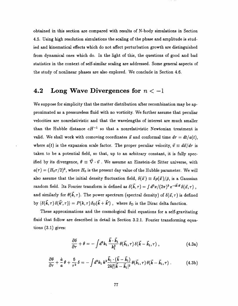
obtained in this section are compared with results of N-body simulations in Section
4.5. Using high resolution simulations the scaling of the phase and amplitude is stud-
ied and kinematical effects which do not affect perturbation growth are distinguished
from dynamical ones which do. In the light of this, the questions of good and bad
statistics in the context of self-similar scaling are addressed. Some general aspects of
the study of nonlinear phases are also explored. We conclude in Section 46.
4.2 Long Wave Divergences for n < -I
We suppose for simplicity that the matter distribution after recombination may be ap-
proximated as a pressureless fluid with no vorticity. We further assume that peculiar
velocities are nonrelativistic and that the wavelengths of interest are much smaller
than the Hubble distance cH-1 so that a nonrelativistic Newtonian treatment is
valid. We shall work with comoving coordinates and conformal time d- = dtla(t),
where a(t) is the expansion scale factor. The proper peculiar velocity, _= dild is
taken to be a potential field, so that, up to an arbitrary constant, it is fully spec-
ified by its divergence, =_ V We assume an Einstein-de Sitter universe, with
a(,r = (Hor/2)2, where Ho is the present day value of the Hubble parameter. We will
also assume that the initial density fluctuation field, X-) =_ 8p(X-)1p, is a Gaussian
random field. Its Fourier transform is defined as 8(k,,r = f dx/(27r )3 e-k�5 5x-,,r)
and similarly for O(k, -r). The power spectrum (spectral density) of 4,r) is defined
by (8(k,,r) 5(k',,r) = P(k,,r) 86(k + W) , where SD is the Dirac delta function.
These approximations and the cosmological fluid equations for a self-gravitating
fluid that follow are described in detail in Section 32.1. Fourier transforming equa-
tions 3.1) gives:
a8 3k k ki+ 0 Id � � k, k kj, -r) (4.3a)2 0 O 8- -(9,r ki
ao 'a 6 g Id3kj k2 ki (k - ki) -�7r + - - :;-- 0kl,,r) O(k - 1,,r) (4.3b)
Ir 2k, 21 k' 12
77
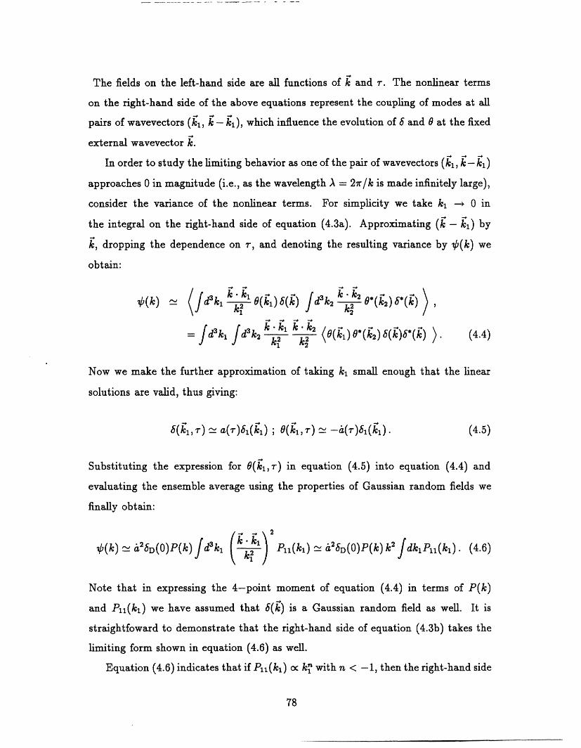
The fields on the left-hand side are all functions of and r. The nonlinear terms
on the right-hand side of the above equations represent the coupling of modes at all
pairs of wavevectors ki , k kj), which influence the evolution of and at the fixed
external wavevector k.
In order to study the limiting behavior as one of the pair of wavevectors (l, k k)
approaches in magnitude (i.e., as the wavelength A = 27r/k is made infinitely large),
consider the variance of the nonlinear terms. For simplicity we take k, -- in
the integral on the right-hand side of equation (4.3a). Approximating - 1 by
k, dropping the dependence on T, and denoting the resulting variance by Ok we
obtain:
3kj � � k, k d3k2 0*(k2) 8*(k)d k 0_ 8A A;2 k21 2
3 3 k '11;2 O(kj)O*(-)8(-8*(-)jd A;, jd J A;2 R k2 k) k (4.4)
1 2
Now we make the further approximation of taking k, small enough that the linear
solutions are valid, thus giving:
6(kl,,r) a(T Xi(kj) 0klT) -ii('081(kj). (4.5)
Substituting the expression for 0k,,T) in equation 45) into equation 44) and
evaluating the ensemble average using the properties of Gaussian random fields we
finally obtain:
k-ki 2V;(k) i25D(O)pM jd3kj k2 P11(ki) _ 26D(O)p(k) 2 jdkjPjj(kj). 46)
1
Note that in expressing the 4-point moment of equation 44) in terms of P(k)
and P1(ki) we have assumed that 6k) is a Gaussian random field as well. It is
straightfoward to demonstrate that the right-hand side of equation (4.3b) takes the
limiting form shown in equation 4.6) as well.
Equation 4.6) indicates that if Pi, (ki) OC kn with n < 1, then the right-hand side1
78

diverges due to contributions from low k. Thus a simple examination of the nonlinear
terms in the cosmological fluid equations by substituting the initial istribution of the
density and velocity field demonstrates the possibility of long wave divergences. These
divergences can potentially be present in solutions for 8(k,,r) and O(k,,r) obtained
from these equations. It is not possible to make any definitive statements, however,
because these are two coupled differential equations - it is necessary to first separate
the equations for and 0, and then identify the nonlinear terms that affect the
amplitude and phase of each quantity (since they are complex variables) to determine
whether the divergent terms affect a particular statistic of interest. This is done in
two different ways in Sections 43 and 4.4.
Before proceeding with a formal analysis of the divergent nonlinear pieces, we
make the connection between the divergent nonlinear terms to the advective (V )
terms in the real space equations. By tracing back the nonlinear terms on the right-
hand side of equations 4.3) to the fluid equations in real space it can be seen that the
terms which contribute to equation 4.4) arise from the V8 and VV- terms. It
is easy to see why such terms should diverge by examining the relation of the power
spectrum of the peculiar velocity to that of the density in linear theory. Using the
linear solutions of equation 4.5) and the definition O(i,,r) -,6(X-,,r), gives,
2Pi 1 . (k 7 = &,'Pi 1 (k) / k (4.7)
where Pll,,,(k) is the linear power spectrum of the peculiar velocity. The rms bulk
velocity on a scale x - k1, Vb(X, r), is given by integrating P(k) over k with a
window function W(kx) (just as one integrates over P(k) for the rms smoothed density
contrast):
Vb(X,,r )2 dkP,,,,(k,,r )W2 (kx) = iL2 47rfdkPjj(k)W2(kX). (4.8)
Since W(kx) - I as k ---+ (see for example the top-hat window function in equation
(3.24b)), the integral on the right-hand side of equation 4-8) diverges at low k for
n < -I in the same manner as the integral in equation 4.6). Thus via the advective
79

(v.V) terms in the fluid equations, the divergence of the non] near terms demonstrated
in equation 4.6) can be traced to the bulk velocity field on a given scale receiving
divergent contributions from k -+ 0, i.e., from the long wavelength modes.
We can now understand why this divergence may not affect self-similar scaling:
the bulk velocity field does not in general have any influence on the growth of pertur-
bations on small scales. In particular, large contributions to the bulk velocity field
from long wave modes correspond to an almost uniform translation of the fluid, and
therefore should not couple to the evolution of at all. This reasoning, and indeed
the entire analysis of this section, relies on making plausible connections of linearized
statistics for and to their nonlinear dynamics. Therefore, while it provides a use-
ful guide to one's intuition, it does not substitute for a rigorous examination of the
nonlinear dynamics.
4.3 Self-Similarity and Perturbation Theory
4.3.1 Formalism
The basic formalism for perturbation theory has been developed in Section 32. Here
we use that formalism to explicitly show that, in the absence of long wave divergences,
perturbative contributions to the power spectrum preserve the standard self-similar
scaling of equation 4.2). At sufficiently small scales 8pl > even at the earliest
times - hence the perturbative expansion breaks down at these scales. This means
that even in the absence of a divergence as --+ oo a high-k cutoff, , must be
used to truncate the perturbative integrals. The requirement of a cutoff restricts the
nonlinear effects that can be studied perturbatively. Nonlinear contributions from
wavenumbers q > k,, cannot be evaluated, but the contribution to any (from all
q < k) are calculable.
It is interesting to note that provided the contributions to P(k) from low q are
convergent, a perturbative expansion can be consistently defined such that the self-
similar scaling of equation 42) is obeyed. This is achieved by defining the high-
80

k cutoff k to be time dependent such that: k,,(,r) oc k.(-r) oc al/(3+n) . With
this scaling, we now show that at all orders in perturbation theory the nonlinear
contribution to the power spectrum takes a self-similar form with characteristic scales,
denoted by kc(T), obeying k(T) o a/(3+n). This should not be surprising since,
once k,(T) is chosen to scale with k,.(,r), there is no other scaling in the problem. We
proceed by obtaining the functional dependence of perturbative contributions on k
and , without needing to know them explicitly. Without loss of generality, consider
the contribution to P(k,,r) from the term (6�, (k,,r) T)), with < m < and
I being even. This contribution is denoted P,j_,n(k,,r) and is defined in equation
(3.13). We substitute for 81 and b;n in equation 3.13) to obtain:
Pnl -,, (k, -r = a d3q, ... dq(1-2) Siol) ... (k q --- i-1) 810m) ...
81 qm q(1-2))) Ml q, ... q(1-2)) (4.9)
where Ml is a dimensionless function of F,n) and F(') which are defined in equations
(3.10). Note that we have already set the arguments of the two 8's opposite to each
other, so that the expression on the right-hand side above has dimensions of a power
spectrum. On taking the ensemble average, the (I - 2 independent phase factors
contained in the functions qj) must cancel pairwise for the result to be non-zero
(recall that the 81's are taken to be independent Gaussian random variables). Thus
we obtain (I - 22 Dirac-delta functions which reduce the number of integration
variables to (I - 22. 12 powers of P(qi = A are also present. Collecting the
relevant factors which provide the k andr dependence, and imposing the high-k cutoff
k,,(T), we obtain
P.,,-, (k, T = a' k3(1-2)/2+nl/2 M2(ku (T)lk), (4.10)
where M2 is another dimensionless function. Taking ku(T) =qa where is a
constant, and introducing a new dimensionless function M3, we finally obtain
PmI-m (k, T = a/(3+n) M3(k 77a 2/(3+n)). (4.11)
81

Equation 4.11) gives the desired self-similar form for characteristic scales kr(r) de-fined by setting kP(k,,r = 1: kr 1/(3+n) (4.2).
.(-r) o a in agreement with equation
Thus at every order in perturbation theory the self-similar scaling of the power
spectrum, and therefore of physical measures of perturbation growth such as the
smoothed density contrast in real space constructed from it, is preserved. However,
this scaling is broken if the perturbative integrals diverge as -+ 0, thus requiring a
low-k cutoff. This possibility is considered next.
4.3.2 Long Wave Divergences in Perturbative Contributions
We showed in Section 32 that at second order in the power spectrum there are terms
that are divergent for n < 1 due to the contribution from k --+ 0. The two however
cancel each other. This cancellation does not prove there is no divergence in the power
spectrum. We must investigate higher-order terms 8 (k ). It is tedious to evaluate the
full expressions for 1 for I > 2 and then to form the power spectrum contributions
Pnl-,n(k). However, we do not need the exact nonlinear power spectrum if we are
interested only in determining whether leading-order long wave divergences are can-
celed. In this case, it is sufficient to work from the outset with only the leading-order
divergent parts of 81(k).
Iterating equations 37) and 3.8), one finds that the leading-order divergences
arise from the term with m = in equations 3.7), with the contribution doubled
in equation (3.7b) because of the term m = I - 1. The leading-order divergent
contributions are then
AI(k - 61-1 k Ck , BI(k - 201-1 k k k d3q 51 (4.12)q2
The leading-order ivergence appears at q 0 in the function C(k). Using equation
(3.8) and iterating we now get the leading-order divergences of 1 and 01:
1-1
81(k) 0(k) 81(k) (4.13)
82
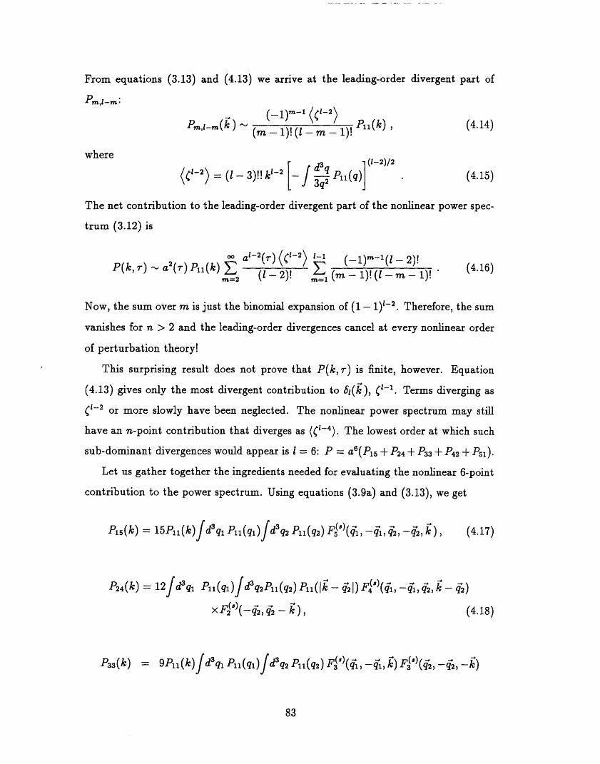
From equations 313) and 413) we arrive at the leading-order divergent part of
P.,i-. (A;) - (M Pi i M (4.14)
where(1-2)/2
(CI-2) = (I - 3! k1-2 d3 P(q) (4.15)3q2
The net contribution to the leading-order divergent part of the nonlinear power spec-
trum 3.12 is
2(,r) p at-2(,r) ((I-2) 2)!P(k,,r - a 11(k) -(I 2)! (M - 1)! (1 M (4.16)
m=2 M=1
Now, the sum over m is just the binomial expansion of ( _ 1-2 . Therefore, the sum
vanishes for n > 2 and the leading-order divergences cancel at every nonlinear order
of perturbation theory!
This surprising result does not prove that P(k, -r) is finite, however. Equation
(4.13) gives only the most divergent contribution to 81(k), (". Terms diverging as
(1-2 or more slowly have been neglected. The nonlinear power spectrum may still
have an n-point contribution that diverges as (CZ-4). The lowest order at which such
sub-dominant divergences would appear is I = 6 P = a(P15 + P24 P33 P42 51)-
Let us gather together the ingredients needed for evaluating the nonlinear 6-point
contribution to the power spectrum. Using equations (3.9a) and 3.13), we get
P15(k = 15P11(k) d3q, P1(q1) d 3q2 P1 1 (q2) F(s) (q-1, - q-1, q- q-2, k (4.17)
P24(k = 12f d3q, P(ql)fd3q2Pl(q2)Pll(lk-q2l)F4s)(ql,-qlq2,A;-q2)
x F2(') 42 - (4.18)
P33(k = 91(k) d3qPll(ql) dq2Pl(q2)F3-')(ql,-q,,k)F(')(q2,-q2,-k)f f 3
83

+6 d3qPll(ql)fd3q2Pl(q2)Pll(lk-q,-q-1)1 2
xF3""(qj I q2 k - q - Q F3""(_qj, -6, q + q - (4.19)
The factors of 15, 12 9 and 6 in equations 4.17)-(4.19) come from the number of
equivalent graphs obtained by relabeling the internal wavevectors, assuming that F(')
and G00 are fully symmetric in all their aguments.
To make further progress we must evaluate 3, 4, and 5. With increasing
the full expression for F(q-,,..., q') rapidly becomes unwieldy. We have attempted
to evaluate some of the divergent terms in equations 4.17)-(4.19). By examining
the form of the sub-dominant divergent parts of the contributing terms, it appears
that the second term in P33 Mst cancel with the divergent part Of P24 as q --+ 0
(and the other terms shown must cancel separately), if the net contribution at this
order is to be convergent. We evaluated these divergent pieces using the "Maple"
package for symbolic mathematics, and had tentatively concluded that the two terms
did not cancel. However we were not able to check our calculations, and due to the
computational complexity involved, did not pursue them further.
The results from the analysis of perturbation theory are therefore not conclusive.
The cancellation of leading divergences is certainly suggestive of an underlying kine-
matical effect which appears in the power counting assessment of the divergence, but
cancels out on computing the net dynamical influence on the power spectrum. We
will interpret this cancellation by examining the phase of 8(k) in Section 44. However
it is not feasible to evaluate all the divergent terms at arbitrary order in perturbation
theory, therefore we pursue a somewhat different approximation to evaluate long wave
mode coupling in the next section.
84

Coupling
The approach in this section relies on assuming that the nonlinear terms in the
Fourier space cosmological fluid equations 43) are dominated by the coupling of
long wave modes. With this ansatz the mode coupling contribution is estimated and
then checked for self-consistency. This allows us to obtain a leading order solution
for the phase shift as described in Section 4.4.1. To make further progress we need to
make the additional assumption that at low k, the Fourier space density and veloc-
ity fields are continuous and therefore amenable to a Taylor series expansion. This
analysis is presented in Section 44.2, and its limitations are iscussed.
4.4.1 Solution for the Phase Shift
In equations 4.3) the integrands on the right-hand side involve products of and
evaluated at ki and k - k1). Let
6(k ki = ) +E(k) ki) Ok ki = W + Wk, kj), (4.20)
where and are unknown functions. In this section we shall use "function" to
refer to random valued fields as well. We shall also suppress the time dependence of
8(k,,r) and of O(k,,r) for convenience (though when we introduce the near solutions
the T dependent part will be explicitly written). Substituting equation 4.20) into
equations 4.3) gives,
3kj+ OW = -id 0(ki) k2 [8(1-c + q, k-1) = Ak), (4.21a)
00( a ki (k - 1) - [0(- +-O(k)+-8(k)=_ d3kj k2 = -2 21 112 Oki) k) k, k, k).a Ir 2k, k
(4.21b)
In order to estimate the nonlinear effects of long wave modes we assume that the
85
4.4 Analytic Approximation for Long Wave Mode

integrands on the right-hand side of equations 4.21) are dominated by the contri-
bution from ki < k. We then approximate O(ki) by the linear solutions given in
equation 4.5): 01(k,,,r = -ii8i(kl), because for k < k the amplitude of the den-
sity perturbations is taken to be very small. Thus we write the right-hand side of
equations 4.21 as
3k,.ki I. k - 3kl.ki kA(k = i S(k) d 2 81 (kJ) it id k2 8kl),E(k ,ki), (4.22a)
3k,.ki A; 3kl -1 A;B(k) =.iO(k) id k2 8ki) +itfd k2 81(ki) W(k , ki). (4.22b)
1 1
In the expression for B(k) we have multiplied the right-hand side by 2 to include
the contribution from (k - 1) -- 0 as required by the symmetry of the integrand.
We have also explicitly written out the dependence of 0k_1), so that 81 (kl) does not
depend on r. We now define the integrals:
k1 8(--i Jd3ki - kJ) (4.23)k2
where i = V�'-__1; and,
k ki 8(_ W(- 6 k kik) ki k ki ki k k (4.24)E( = ii f d3k, k2 k) d3k, 7C2 M , 1)1 1
Using these definitions equations 4.21) can be written as:
a8(k)a-r + O(k) = i ii k 5 8k + Ek) (4.25)
'90(k) -a - 6 -+ - OM + - 6(k = a k O(k) + W(k).r a 2 (4.26)
The above equations are exact aside from using the linear solutions for 0kl in
the right-hand side of equations 421). We have defined al in equation 4.23 so
that it is purely real. This can be verified by using the relation of 1 to its complex
conjugate: 81(ki = -ki), which is required to ensure that 8(i) is real. The reason
86

for introducing is that it is independent of k and r, therefore, given the initial
density 1, it can be treated as a numerical constant.
We now turn to the issue of long wave ivergences. The variance of - is:
2) 3kj P11(ki)(a Ck d 47r dkPll(A;,). (4.27)k21
Thus (a2) is a ivergent integral for n < 1. To proceed further we need to estimate
the degree of divergence of the integrals Ek-) and W(k). We do so by using equation
(4.20) to substitute for and in E and W. The resulting expression for the variance
of E is:
2 3kj 3k k ki k k2(JE(k)l a2 d d 2A;2 k2
1 2
61 ki) 8( ) [6(k - k1 - 8(k)] [8*(k- - k2 - k)] ).(4.28)
To simplify this expression we assume that for the purposes of assessing the degree of
divergence, a the fields involved are well approximated by the linear solution. Then
the expectation values can be evaluated using the properties of Gaussian random
fields. Of the twelve terms that result, the leading contribution in the long wave Emit
arises from the term with (1 k 81'(- (8(k - Icj)8*( - k2)) in the integrand. This
contribution is:
(I E(k)12) i2 P (k) SD (0) k2a2. (4.29)3
The variance of the first term on the right-hand side of equation 4.25), iizi is
exactly the same as the above result for E(k-) 12) , hence both terms must be retained
at the same order in evaluating the long wave contribution. Likewise, it is easy to
show that W in equation 4.26) is of the same order as the first term on the right-hand
side, and is also proportional to a in its degree of divergence.
Equations 4.25) and 4.26) can be re-written as a pair of second order differential- . ),equations in for and . For the result is (with a
+ _,i2 &2 6 ii3iii - - _ E + ia&E + W 0. 430)a T2 a
87
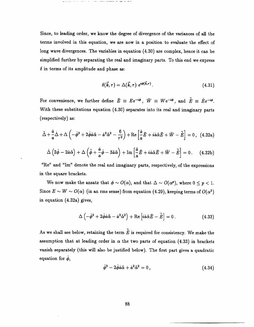
Since, to leading order, we know the degree of divergence of the variances of all the
terms involved in this equation, we are now in a position to evaluate the effect of
long wave divergences. The variables in equation 4.30) are complex, hence it can be
simplified further by separating the real and imaginary parts. To this end we express
8 in terms of its amplitude and phase as:
6(k,,r) A(k,,r) e (4.31)
For convenience, we further define Ee-i'O, V We-"O, and E te-io.
With these substitutions equation 4.30) separates into its real and imaginary parts
(respectively) as:
il&2 6 it+ + 2 + Re 2 + ia&B + V E = 0, (4.32a)a 7 a
a� a -(2 - Ii&) A a - + Im a E+ib&E+W-E =0. (4.32b)
"Re" and "Im" denote the real and imaginary parts, respectively, of the expressions
in the square brackets.
We now make the ansatz that O(a), and that A - 0(aP), where < p < .
Since E - W - O(a) (in an rms sense) from equation 4.29), keeping terms of (a2)
in equation (4.32a) gives,
A -_�2 + 2,i - i2&2) + Re [iit&E - E = . (4.33)
As we shall see below, retaining the term E is required for consistency. We make the
assumption that at leading order in a the two parts of equation 433) in brackets
vanish separately (this will also be justified below). The -first part gives a quadratic
equation for ,
2 - 2 ,i& + 2&2 = (4-34)
88

which has the solution, a = d a'. Thus the leading order solution for is:
0(k-,,r = a(,r) al + (4.35)
where k) is the value of the phase at the initial time.
The solution of equation 4.35) can be used to justify the assumptions that have
been made. Firstly, is indeed of O(a), as assumed at the outset. Further, equations
(4.24) and 4.35) can be used to simplify the expression for E and thereby justify
setting the first part of equation 4.33) to separately. To start with let us write E
in terms of A and :
(4.36)io(k)E =,ifd3ki A;2 Ai(kJ)e k k, kI
Differentiating equation (4.36) with respect to and multiplying by e-i'O(k) gives,
a 3k, k k k, k k,E _.B+,ifda k21
x f A(k) + Aw�w I (4-37)
The leading order terms on the right-hand side above are the two terms with �: they
are at least of O(a 2). However, by substituting = into equation 4.37), and
comparing with the expression for that follows from equation 4-36), it can be seen
that these leading order terms exactly cancel the contribution from iii&B in equation
(4.33). Thus the surviving terms in the second part of equation 4.33) are a of lower
order than O(a2) - therefore they can be neglected in comparison to the first part
of the equation which was used to get the solution for of equation 4.35). This
establishes the consistency of the approximations used to obtain this solution.
The variance of the phase shift given by equation 4.35) is:
. . 22 3kJ (k. ki )
a(,r)2,k2 A;2 P11(ki), (4.38)
where 50(k,,r) = O(k,,r - k), and k and k, are unit vectors. Since k is a fixed
89

external vector the angular integral can be performed so that the final result depends
only on the magnitude of :
[go(- r) 2 47r k2T a(,r)' dk-, Pi (c, (4.39)
Thus the leading order solution for 6(k) involves a growing (divergent) phase shift,
but there are no contributions to the amplitude at this order. The above analysis can
be repeated for the velocity divergence 0k) to verify that the leading order result for
Ow is the same, with equation 4.35) giving the solution for its phase as well. These
results were obtained by retaining terms of (a2). Since divergent terms of 0(CX) are
also present in the equations we cannot say anything conclusive about the degree of
(possible) divergence of the amplitude k). In the following section we shall address
this question by expanding the equations to next order in a with some additional
assumptions.
The solution 4.35) for the phase shift has a simple physical interpretation. As
noted in Section 42, the linear bulk velocity Vb diverges due to contributions from long
wave modes (equation 4.8)). The limiting form of the integral given in equation 4.8)
for v 2, and that of equation 4.39), is the same. This connection can be made more
precise by imagining a single sine-wave density perturbation in real space: X-' -r)
60 sin(k- -. Now suppose that the fluid in which this perturbation is made is moved
with a uniform translational velocity of magnitude Vb(,r) given by 4.8) (the scale x
in equation 4.8) has no connection to the spatial variable used here). The distance
moved by each fluid element is f dr Vb(,r = Vb(-r) a(,r)/a(,r), where we have used
Vb(,r) oc it(,r). If the coordinate frame is kept fixed relative to this translational
motion, then the density perturbation will acquire the following time dependence due
to the bulk velocity: x r = o sin Vba/iz)], where is the direction of the
bulk velocity. Therefore acquires a phase shift: 80(k = k - a/it Vb- On squaring,
and averaging over angles between and 6 this gives:
- 2 1 a2[80(k T) - - k2 V2(,r). (4.40)3 j12 b
90

Note that the averaging over angles is consistent with the angular integral done to get
equation 4.39), and amounts to estimating the typical phase shift due to a superpo-
sition of bulk flows of magnitude Vb directed randomly with respect to k. Substituting
for v from equation 4.8) and assuming it is dominated by the contribution from lowb
k, we recover the result in equation 4.39). Thus we have shown that for n < 1
the dominant phase shift is due to the kinematical effect of the bulk motion on small
scales imparted by long wave modes. This is consistent with the connection between
divergences in the nonlinear terms in the fluid equations and Vb made in Section 42.
4.4.2 Taylor Series Expansion
In this section we make an additional assumption about the k-dependence of 8(k)
and O(k): we assume that at small k, 8 and are smooth functions of k with a well
defined derivative with respect to k. With this assumption we expand the nonlinear
integrals in equations 4.3) in a Taylor series in (ki/k) about and restrict the range
of integration to small kj. Thus we write: k - k1) 8(k - ki a8l,9k, and likewise
for O(k - k). Unfortunately, the standard assumption about and in cosmology
is that they are Gaussian random fields at the initial time. Thus at each value of
k they are given by a random number drawn from a probability distribution. The
distribution of or with respect to k is quite the opposite of a smooth function,
because its values at any two k are uncorrelated. We return to this point later in this
section and in Section 46, but here we proceed with the Taylor series approach.
With the Taylor expansion described above, the right-hand sides of equations
(4.3), denoted by Ck) and D(k), take the form:
CM Id3k, 0) V 6(k) ki + 0k)8(ki) + (4.41a)
2-k 2(ki . ) k, - k - '90(k)D(k) d3k, 0k,) O(k) + O(k - --p-kj -r- ... ,k2k2
(4.41b)
where both equations have been expanded to the same order. In equations 4.41 we
91

have included the contributions from (k- - k-,) -+ 0 as well. We now write equations
(4.41) at the order shown as linear equations by appro,,dmating and at small k,
by the linear solutions 1 and 01. Recall that we had obtained one linear term on the
right-hand side of each equation in the previous section by introducing the integral
Oe. Here we introduce three new integrals: q, -f and gij,
Id 3A;18(- d3k,[2(k -ki )2 _ 1]8(- d 3kjkjjkjj6(k-j), (4.42)ki) -Y ki) gj
where k1i and 1j denote the ith and jth components of the vector j, so that gij
is a tensor. Note that aside from the dependence of -y on the direction of all the
integrals in equation 4.42) are independent of k and T. In addition, all the integrals
are convergent in an rms sense for n > 3.
We proceed by writing down a second order differential equation for in terms of
C and D:a 6 a
- - = C + -C + D. (4.43)a T2 a
We then use the definitions of equation 4.42) to rewrite equations 4.41) as:
CM = iLk Cx + iL[kjgjjaj] - a770, (4.44)
and
D(k = ibk -0 - L[kjgjjaj] - &yO, (4.45)
where a =_ 91akj, and the repeated indices i and j are summed over. We will now
attempt to solve these equations for the amplitude and phase of to a given order
in a. We begin by using equations 4.44) and 4.45) to eliminate in the terms on
the right-hand side of equation 4.43) (we will also need to use the left-hand sides of
equations 4.3)). Some algebra yields the following equation for :
+ -ya - 2za - - 2a(kjgjiaj) 6 (1 + a7)8a I T2
C - '(kjgjjailn6)]2 _ iL2 z 21nS 6[-k-gijCx + '(kgijaj) I
92

a2Ik 6 - i(kjgjj(9IIn6)j -ya + j2 8= O. (4.46)
a 1 + aq
We now make a WKB analysis, which relies on taking the phase to be more rapidly
varying than the amplitude, to obtain self-consistent equations for the amplitude and
phase. After some algebra we get the following relation for by solving equation
(4.46) at 0(a 2):
=gk- a igipajo). (4.47)
This yields the solution,
= kTFa + 0 ; F = egg-'(l - e -ag), (4.48)
where al has been represented as a column vector, kT denotes a row vector representing
k, and g and F are 3 by 3 matrices, with I being the identity matrix. This solution
can be verified by substitution using equation 4.46). Note that for ag < , F can be
expanded as a Taylor series: F a+ a 2g/2+a 3g2 /6+.... For ag I the leading order
solution is = ak + 0j, in agreement with 4.35). The solution for in equation
(4.48) can be used in equation 4.46) to obtain an equation for A only. After some
algebra, this equation simplifies to:
il I (kigijaj) 6 + iL2+ � � -ya - -2a _(1 + a7)A A(kjgjj8jInA)Ia I aq I 2
jZ 2iL2A(kgja,)2 aa+ In - _(kjgjj,9jInA) ya A = . (4.49)
a 1 + aq j12
Note that in this equation for A, all terms involving i and the divergent integral a
have cancelled out exactly! Hence the solution for A has no dependence on a, the
only divergent integral in equation (4-46). Obtaining the fun solution for A is still not
possible as it requires solving equation 4.49) a nonlinear partial differential equation;
however, for our purpose the key goal was the assessment of the a-dependence of A.
Thus the Taylor series approach leads to two striking results: the solution for the
phase given by equation 4.48), and the result that the evolution of the amplitude is
93

not influenced by any divergent integrals.
The above conclusions thus support the interpretation discussed in Section 42
that for 3 < n < -1, there is no dynamically relevant divergence. Hence the
evolution of scale free spectra will obey the standard self-similar scaling provided the
statistics used are relevant to the growth of density perturbations. The divergent
growth of the phase is not a measure of perturbation growth as it arises from bulk
motions. However these conclusions rest on the assumption of a valid Taylor series
approximation for and 0. This assumption cannot be justified in the cosmological
context for random-phase Gaussian initial conditions. Hence we must still regard
the conclusions of this section as being suggestive of the answer, but not as proven
results.
4.5 Self-Similar Scaling in N-body Simulations
N-body simulations provide a powerful means for testing the self-similar scaling of
scale free spectra. The deeply nonlinear regime is accessible in these simulations,
thus oering the possibility of measuring the complete similarity solution. N-body
simulations have limited dynamic range, but they do not rely on any approximations
of the kind made in Sections 43 and 4.4. Therefore they provide a complementary
technique to the analytic approaches of previous sections. In this section we study
two scale free N-body simulations, n = and n = 2, in order to measure their
scaling properties.
The n = 2 simulation was performed by Ed Bertschinger. It is a particle-
particle/particle-mesh simulation with 128' particles. Data from 21 time outputs of
this simulation were analyzed, with the scale factor a(,r) increasing by a factor of 2/4
between successive outputs. The n = simulation was performed by Simon White.
It is also a particle-particle/particle-mesh simulation done with 1001 particles. Data
were available for 9 time outputs, with the scale factor increasing by a factor of .6
between successive outputs (except for the first two). This simulation is used as a
control case to test the accuracy of the results for the n = 2 simulation. Since
94

n = does not suffer from potential long wave divergences, the standard self-similar
scaling is expected to hold, and has in fact been convincingly demonstrated in earlier
work. Hence the results of this simulation provide a good indication of the degree of
accuracy with which the N-body simulations show the similarity solution (though the
differences in the number of particles and other parameters in the two simulations
complicate such a comparison).
Here we briefly outline the N-body calculation; many relevant details are provided
by Gelb 1992). The particle-mesh calculation of the simulation is done by solving
Poisson's equation on a cubical grid using the fast Fourier transform (FFT). In Fourier
space Poisson's equation is:
47rGpb(,r)a 2'�b (A; r) k 2 (4.50)
where is the Fourier transform of the perturbed gravitational potential. In an
N-body simulation the density is computed using the number density of a finite num-
ber of particles. The real space density is computed on a cubical, three dimensional
grid by interpolating from the particle positions. This density is then Fourier trans-
formed using the FFT algorithm, and thenl�(k,,r) is computed using equation 4.50).
Multiplying 1(k,,r) by Zk (which corresponds to taking a gradient in real space) gives
the Fourier transform of the gravitational force vector. This is transformed back to
real space with three FFTs for each component. The real space forces are then used
to move the particles using the equation of motion in comoving coordinates. This
procedure is interated to continue the simulation. To increase the resolution of the
forces, the force on each particle due to its nearest neighbors is computed by direct
summation using a Plummer model for the force law: F(r = _GM2FI(r 2+ 2)3/2,
where is known as the Plummer softening parameter. It is (1/2560)L for the n = 2
simulation, where L denotes the size of the box.
Thus in the N-body simulations there are many departures from the idealization
of an infinite, continuous fluid. The limitations common to any N-body simulation
are the finite size of the box and the discrete nature of particles. Additional scales
95
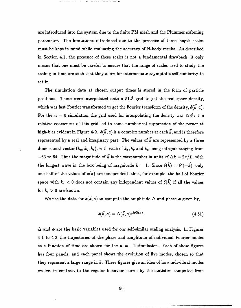
are introduced into the system due to the finite PM mesh and the Plummer softening
parameter. The limitations introduced due to the presence of these length scales
must be kept in mind while evaluating the accuracy of N-body results. As described
in Section 41, the presence of these scales is not a fundamental drawback; it only
means that one must be careful to ensure that the range of scales used to study the
scaling in time are such that they allow for intermediate asymptotic self-similarity to
set in.
The simulation data at chosen output times is stored in the form of particle
positions. These were interpolated onto a 512 3 grid to get the real space density,
which was fast Fourier transformed to get the Fourier transform of the density, 6(k, a).
For the n = simulation the grid used for interpolating the density was 128': the
relative coarseness of this grid led to some numberical suppression of the power at
high-k as evident in Figure 49. 6(k, a) is a complex number at each k, and is therefore
represented by a real and imaginary part. The values of k are represented by a three
dimensional vector (k., ky, k, and k,, being integers ranging from
-63 to 64. Thus the magnitude of k is the wavenumber in units of Ak = 27r/L, with
the longest wave in the box being of magnitude k = 1. Since 8(k = 8*(-k), only
one half of the values of k) are independent; thus, for example, the half of Fourier
space with k < does not contain any independent values of k) if all the values
for > are known.
We use the data for 8(k, a) to compute the amplitude A and phase given by,
a) = A k, a) e (4.51)
A and are the basic variables used for our self-similar scaling analysis. In Figures
4-1 to 43 the trajectories of the phase and amplitude of individual Fourier modes
as a function of time are shown for the n = 2 simulation. Each of these figures
has four panels, and each panel shows the evolution of five modes, chosen so that
they represent a large range in k. These figures give an iea of how individual modes
evolve, in contrast to the regular behavior shown by the statistics computed from
96

them. Thus even at relatively early times when most statistics obey linear behavior,
the amplitudes and phases can be seen to follow quite jagged paths.
A technical problem in the measurement of the phase arises because conventionally
the phases are defined modulo (2,x). The phase trajectories that follow are shown in
Figure 41, where a the phases he between -x and7r. This is how the phases from N-
body data have been computed in previous studies (Ryden Gramann 1991; Scherrer
et al. 1991; Suto & Suginohara 1991). However, a glance at the phase trajectories in
Figure 41 makes it clear that this will have the effect of randomizing the phases at
late times relative to their initial values, even if the growth were monotonic. This is
because even a small change in the phase, 50, could cause it to be mapped to a value
indicating a change of (27r - 01). If the trajectories could be obtained with arbitrarily
small increments in a then such artificial mappings could be un-done, and the phases
plotted without constraining them between -7r and 7r. Since outputs are available
only at discrete values of a, there is a two-fold ambiguity in defining the phase.
Consider the phase values at two successive a's for a given k: O(k, aj) and 0(k, a+,),
defined in the usual way to lie between -7r and 7r. Let 60 = O(k aj+,) _O(k a)
An alternate value for the phase at a+1 is k a+, = Ok, aj) ± (27r - I 0j 1), where
the sign in positive if 80j < and vice versa. To choose between and O', we follow
the trajectory of each mode, and at each successive value of a, we define the phase by
taking the magnitude of the change in phase to be the smaller of 180 I and (27r - 150j 1).
The result is shown in Figure 42. As long as the typical changes in phase at successive
times are less than7r, this procedure is a reasonable way of extending the range of .
As we shall see, this considerably extends the degree of phase nonlinearity accessible
to our analysis.
Following Ryden Gramann 1991) and Gramann 1992), we define the following
statistics as a measure of the degree of nonlinear evolution. For the phase we define the
mean deviation from the initial phase, 50 k, a) =_ (I 80(k, a) 1 = a) - -, a)),
where ai is the initial value of a. The averages indicated are performed over the
different modes within a shell in k-space whose wavenumbers lie between (k-0.5) and
(k + 0.5). For the amplitude we simply measure the mean amplitude (A(k-, a)) within
97

each shell in k-space. The results are plotted in Figures 44 and 45 for n = 2, and
Figures 48 and 49 for n = . These results are interesting in themselves, but here we
limit ourselves to using them to define characteristic wavenumber scales, which are
then used to test for self-similar scaling. For Figures 44 and 48, if we had used the
phase trajectories as shown in Figure 41 (i.e., defined to he between -7r and 7r), then
all the late time curves for (80(k, a)) would have reached a maximum of (27r/3) - this
corresponds to a distribution of 0(k, a) that is uncorrelated with - a). However,
it is clear from Figure 44 that 3 shows systematic growth well beyond 2r/3. Thus
with the phase information that we have generated, previously unexplored aspects of
phase evolution in the deeply nonlinear regime can be addressed.
To analyze self-similar scaling, we define two characteristic wavenumbers. The
first, denoted kc(a, OC), is defined by setting YO(k, a) = OC, where or is a constant.
The second, denoted kC(a, AC) is defined using the amplitude as follows:
IA(k, a) - Al(k- al-= AC) (4.52)
Al k a)
where Ai(k) a) is the linear solution for A, and A is a dimensionless constant. Thus
kc(a, AC) is the wavenumber at which the fractional departure of the amplitude from
the linear solution is A These statistics involve summing the magnitudes of the
departures from linear behavior for each mode within a given k-shell; hence they
probe the degree of nonlinearity more directly than if a statistic was computed first,
and then its departure from the linear solution was calculated.
Figure 46 is a plot of log[kC(a, Oc)] vs. a with n = 2, for 4 different values of
OC. Also shown in the plot are the scalings expected from the standard self-similar
behavior) Ic oc a2/(3+.) oc a-2 for n = 2, and the scaling resulting from the solution
for 80 given by equation 4.35), k oc a-'. The plots show that for Oc =r and r/2,
the latter scaling is closely followed; but for the lower values Oc = r/4 and X/8,
the former scaling is more closely followed. We verified that the trends did reflect a
gradual transition in the scaling of kc(a, OC) by plotting a larger range of Oc down to
OC = 7r/20. This can be interpreted as follows. For a given k, at early times as the
98
phase just begins to depart from the linear solution (in which remains constant in
time), its evolution is dominated by perturbative or other weakly nonlinear efrects.
These effects in general involve the coupling of a range of values of W, mostly in the
vicinity of k = k, and obey the standard self-similar scaling. However at late times
the phase shift is dominated by the bulk flow due to the longest waves in the box.
The resulting phase change is given by equation 4.35) - it is a smooth function of a
and and therefore dominates the other, more stochastic components of the phase
change at late times. Thus the phase shows behavior that we can interpret as arising
from a combination of the kinematical divergence described in previous sections, and
a dynamical, nonlinear component which obeys the standard self-similar scaling. The
results for n = shown in Figure 410 show only one behavior, the self-similar scaling,
k oc a-'/'. This is expected as the linear bulk velocity does not diverge, therefore the
longest waves in the box do not dominate the phase shift.
For the amplitude scaling, Figure 47 shows a plot of log[k(a, A,,)] vs. a with
n = 2, for ,, = 025) 0.5) 1 2 For sufficiently high k, all four curves closely follow
the standard self-similar scaling, k oc a-2 . This is consistent with the indications from
previous sections that the divergence from long waves does not affect the amplitude.
All the curves show a consistent departure from the oc a-2 behavior at low ,
roughly for < This most likely indicates that the absence of power on modes
with wavelengths larger than the box-size has slowed the growth of modes which
would otherwise be enhanced by the former. Thus the standard self-similar solution
for n = 2 is obtained only on scales significantly smaller than the box-size. For
n = the self-similar scaling k oc a-1/3 is again shown convincingly.
Our results are in partial disagreement with those of Gramann 1992). She found
that for n = -1 in two dimensions (the analog of n = 2 in three imensions),
the standard self-similar scaling is broken for both the phase and amplitude. Our
results for the phase scaling are consistent with hers, but the amplitude scalings are
quite different our results show good agreement with the scaling o a whereas
hers agree with kr oc a'. Since the statistics that we have measured were chosen
to agree with her definitions, it is difficult to explain the origin of the isagreement.
99

It is conceivable that there are basic differences in the dynamics in two and three
dimensions, but this is not reflected in the analytical results of Section 44.
4.6 Conclusion
In Sections 41 and 42 we presented arguments outlining the need to examine the
self-similar scaling of scale free spectra, pk) C kn' for 3 < n < -1. It was shown
that terms diverging due to the contribution from long wave modes were present in
the cosmological fluid equations, but that it needed to be determined whether they
had any dynamical influence on the growth of density perturbations.
We have examined this issue through analytical and N-body techniques in Sec-
tions 43-4.5. Our conclusions can be summarized as follows:
(i) In Section 43.2 we examined perturbative contributions to the power spectrum to
examine the possibility of long wave divergences in these contributions for 3 < n <
-1. We found that divergent terms were indeed present, but that the leading order
divergences cancelled out at each order in perturbation theory. Terms which diverged
less strongly are also present, but due to the computational complexity involved we
were unable to analyze them.
(ii) In Section 44 we developed a non-perturbative approximation to study the non-
linear coupling of long wave modes. We obtained a solution for the phase shift whose
variance is divergent for 3 < n < 1. This divergence was interpreted to arise from
the kinematical effect of the bulk flows induced by long wave modes. With additional
assumptions requiring that the Fourier space density be amenable to a Taylor series
expansion around k we showed that the evolution of the amplitude of 6(k a is not
influenced by the divergent terms. It was emphasised that the Taylor series expan-
sion cannot be justified for Gaussian random -fields, and therefore the final conclusion
cannot be regarded as a proof.
(iii) In Section 45 we studied the self-similar scaling of an n = 2 scale free sim-
ulations, and used an n = simulation as a control case. It was demonstrated
numerically that for n = 2 the phase shift indeed obeys a scaling consistent with
100

the solution found in Section 44 at sufficiently late times. At early times the evolu-
tion of the phase shift was consistent with the standard self-similar scaling. Thus the
phase shift arises from a combination of kinematical effects due to large scale flows
which dominate at late times, as well as genuine dynamical effects which dominate at
early times in the weakly nonlinear stage of its evolution. With some further analysis
it may be possible to construct a concrete analytical model to support this interpre-
tation.
(iv) The scaling of the amplitude followed the standard self-similar form, except at
wavenumbers k 10 (in units of 27r/L). This is consistent with the results of Sections
4.3 and 44, and the interpretation that dynamical measures of perturbation growth
preserve self-similar scaling for 3 < n < -1.
It was disappointing that neither of our analytical approaches led to a rigorous
result regarding self-similar scaling of the amplitude of the density. However, in
combination with the N-body results they lead us to conclude with some confidence
that the self-similar evolution of the density contrast is preserved for 3 < n < -1.
The kinematical interpretation for the scaling of the phase shift provides a useful
guide to identifying statistics susceptible to such effects. The rms displacement of
particle postions is another statistic which would be dominated by the bulk motions
from long wave modes for n < -1, and must therefore be used with caution as a
measure of nonlinear evolution.
It is a pleasure to thank Alan Guth for many stimulating discussions which helped
to clarify and sharpen our arguments. We thank Simon White for providing the
results of his scale free simulations, his hospitality at the Institute of Astronomy,
and for several useful suggestions. We also acknowledge useful discussions with Shep
Doeleman, Mirt Gramann, Ofer Lahav, Samir Mathur, Adi Nusser and, especially,
David Weinberg.
101

REFERENCES
Barenblatt G I. 1979, Similarity, Self-Similarity, and Intermediate Asymptotics (New
York: Consultants Bureau)
Bertschinger, E. 1992, in New Insights into the Universe, ed. Martinez, V. J., Portilla,
M. Saez, D. (Berlin: Springer-Verlag), p 65
Bertschinger, E. Gelb, J. 1991, Comp. in Physics, 5, 164
Davis, M. Peebles, P. J. E. 1977) ApJS, 34, 425
Efstathiou, G. 1990, in Physics of the Early Universe, ed. Peacock, J. A., Heavens,
A. F. Davies) A. T. (Bristol: IOP), p. 361
Efstathiou, G. Eastwood, J W. 1981, MNRAS, 194, 503
Efstathiou, G., Frenk C S., White, S. D. M., Davis, M. 1988, MNRAS, 235, 715
Gelb, J. M. 1992, PhD. Thesis, M.I.T.
Goroff, M. H., Grinstein, B., Rey, S.-J. Wise, M. B. 1986, ApJ, 311 6
Gramann, M. 1992) ApJ, 401 19
Klypin, A. A. Melott, A. A. 1992, ApJ, 399, 397
Makino, N., Sasaki, M. Suto) Y. 1992, Phys.Rev.D, 46, 585
Peebles, P. J. E. 1974) A&A) 321 391
Peebles, P. J. E. 1980) The Large-Scale Structure of the Universe (Princeton: Prince-
ton University Press)
Peebles, P. J. E. 1993, Principles of Physical Cosmology (Princeton: Princeton Uni-
versity Press)
Press, W. H. Schechter, P 1974) ApJ, 187, 425
Ryden, B. S. Gramann, M. 1991, ApJ, 383, L33
102
Scherrer, R. J.) Melott) A. L. Shandarin, S. F 1991) ApJ, 377 29
Suginohara, T. Suto Y 1991, ApJ, 371, 470
Vishniac, E. T. 1983, MNRAS, 203, 345
Zel'dovich, Ya. B. 1965, Adv. Astron. Ap. 3 352
103

4
2
4 0_19-
-2
-4
4
2
I-t-i-v. 0-9-
-2
-4
0 .2 .4 .6 .8 1 0 .2 .4 .6 .8 1a(r) a(-r)
4
2
.4i 0
-2
-4
k=1-54
2
i-i1.2 0
-2
-4
0 .2 .4 .6 .8 1 0 .2 .4 .6 .8 1a(T) a(T)
Figure 41 The trajectories of the phases 0(k,,r) of individual Fourier modes forn = 2 axe plotted vs. a(r). The magnitudes, k, of the wavevectors are labeled ineach panel; the full vectors were chosen as = , 0, k). Within each panel increasesin the following order: solid, dotted, dashed, long-dashed, dashed-dotted curves. Thephase is defined modulo 27r, and is therefore constrained to lie between -7r and 7.Outputs at 21 values of a have been used to plot each trajectory. At a = 0, the valueof 0 at the earliest time has been plotted again to show the expected linear behavior.
104

I I I I I I I r
k=21-25 71 1 1 1 1 1 1 1 1 1
- - - - - - - - - - - - - - - - - - -D .2 .4 .6 .8 1
a(T)
77-
10
5
10
5r-
7I7 --- ,
1-1
I
'-. I--">,17 ". _. 1-1
Y'
7
.1iI.-,_19-
-i1-1-9-
0 0
-5
-10
10
5
0
-5
-10
-5
-1071 1 I I I I I I I I I I I I I I I I
I 0 .2 .4 .6 .8 1a(-r)
10
5
0
-5
-10
_I__T _ [ T FI - I F F1 T FFT_
k= 1-5
0 .2 .4a(r)
6 .8 0 .2 .4 .6a(-r)
.81 1
Figure 42 The same trajectories as in Figure 41 are plotted, but has been re-defined so that it is no longer constrained between -7r and 7r (notice the limits onthe y-axis). To overcome the modulo 27r constraint, the phase at each time output isdefined by adding to the previous value of the phase the change in phase which is thesmaller of two choices as described in Section 45. In linear theory the phases do notcha.uge with time; significant departures from this can be seen in all but the lowest modes.
105

.03 .02
.02
.01
n
.015
1-1i.:se .0 1I-
.005
n0 .2 .4 .6 .8 1 0 .2 .4 .6 .8 1
a(T) CL(T)
A ff.
.08
.06
.04
.02
n
.UD
.04
- .031-iQI-
.02
.01
n0 .2 .4 .6 .8 1 0 .2 .4 .6 .8 1
a(-r) a(-r)
Figure 43 The trajectories of the amplitudes k,,r) of individual Fourier modes forn = 2 are plotted vs. a, as in Figure 41 for the phase. Note that at early timesA oc a: to check this a the curves have been joined to A = at a = . Thereforethe lowest value of a at which epartures from a straight line occur shows nonlinearbehavior.
106
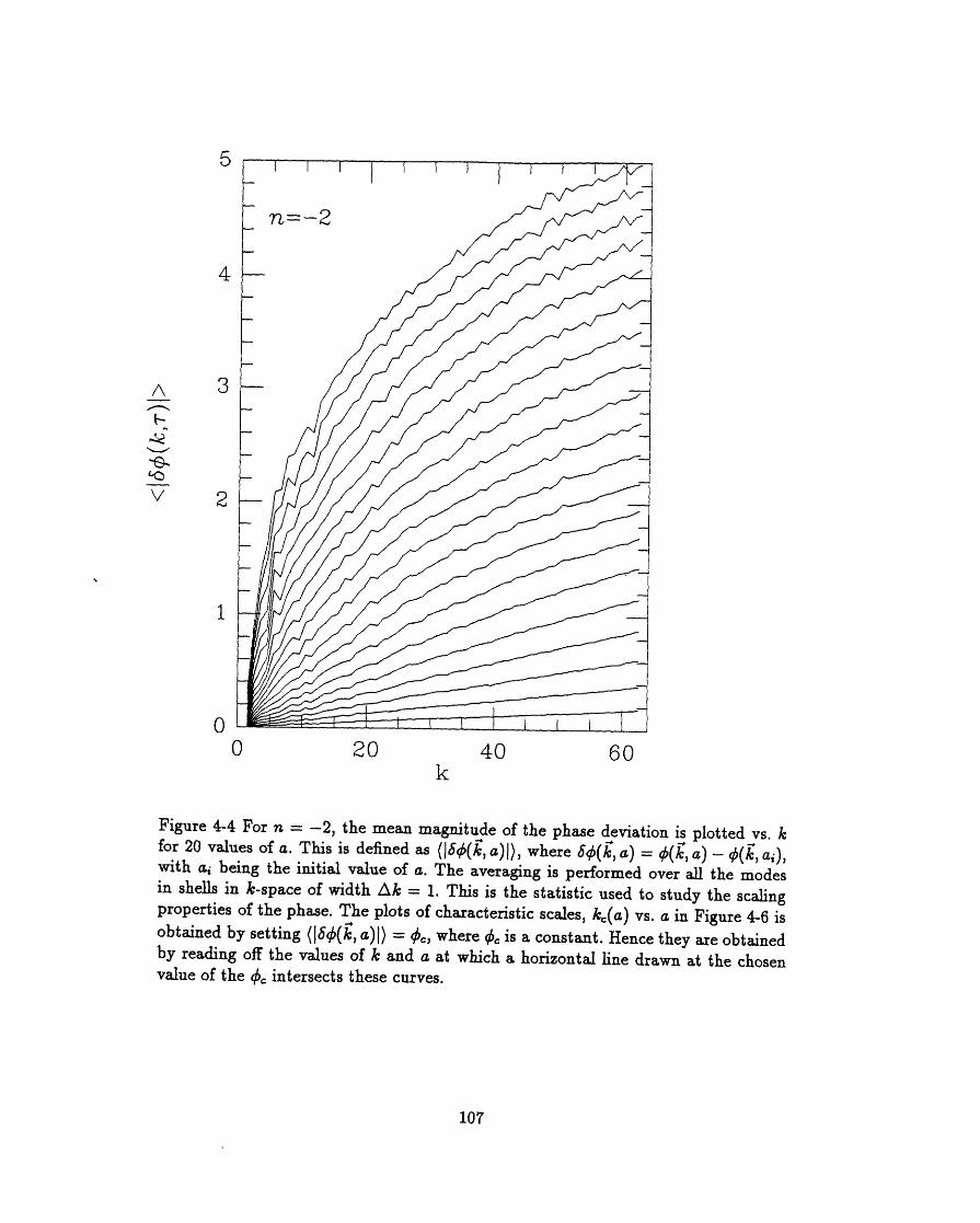
5
4
A 3
4�-E�LC
V 2
1
00 20 40 60
k
Figure 44 For n = 2, the mean magnitude of the phase deviation is plotted vs. for 20 values of a. This is defined as (I 0k, a) 1), where 80(k, a) = O(k, a) - k a),with ai being the initial value of a. The averaging is performed over all the modesin shells in k-space of width Ak = This is the statistic used to study the scalingproperties of the phase. The plots of characteristic scales, k(a) vs. a in Figure 46 isobtained by setting 180(k, a) 1 = or, where is a constant. Hence they axe obtainedby reading off the values of k and a at which a horizontal line drawn at the chosenvalue of the intersects these curves.
107
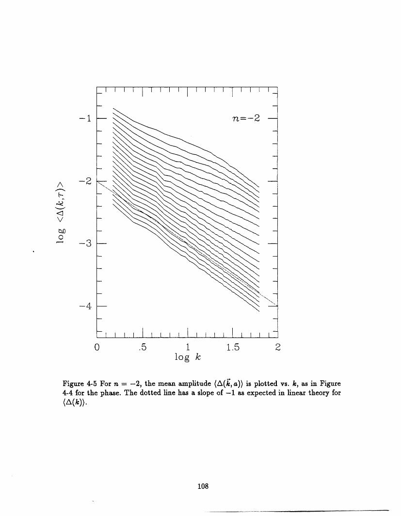
1
A -2
112I.-I
V
to0
4 -3
-4
0 .5 1 1.5 2log k
Figure 45 For n = 2, the mean amplitude (A(k, a)) is plotted vs. k, as in Figure4-4 for the phase. The dotted line has a slope of -1 as expected in linear theory for(A(k)).
108

2
1.8
1.6
1.411-1-6-CT
42 1.2to0
1
.8
.6
-1.4 -1.2 -1 -. 8 -. 6 -. 4 -. 2 0log a
Figure 46 For the n = 2 spectrum, the scaling of characteristic wavenumber scales,k, vs. a is shown, as derived from the mean phase deviation. As described earlier inFigure 44, c,, (a, ) is the value of and a at which (I 60(k, a) 1 = Oc. The four solidcurves correspond (from top to bottom) to the values of Oc labelled at the top of theplot. Note that for high values of (the top 2 curves), the scaling closely agrees withthat derived from equation 4.35): k, oc a-', which is shown by the upper dotted line.
-2A transition towards the standard self-sin3ilar scaling k o a shown by the lowerdotted line, occurs for the 2 lower values of 0,.
109

2
1.8
1.6
1.4I-.:I
I-,
11.2 1.2to2
1
.8
.6
-1.4 -1.2 -1 -. 8 -. 6 -. 4 -. 2 0log a
Figure 4-7 For the n = -2 spectrum, the scaling of characteristic wavenumber scalesderived from the departure of the amplitude from linear growth, k'r(a, A,,) vs. a isshown for 4 different values of A, (see equation 4.52) for the efinition of k"(a, A,,)).All the curves have a slope close to the standard self-similar scaling, k oc a-2 at highk. For k below about 10 the slope becomes shallower, probably due to the limitationof a finite box.
110

5
4
A 3d
-�21--,-G-CC
V 2
1
n0 20 40 60
k
Figure 48 Mean phase deviation for n = : this is the counterpart of Figure 44 forn = .
ill

1
Ad -2
-Y1--,
vZ:W0
,---I
-3
-A I I I I I I I I II I I I I I I I I I
0 .5 1 1.5 2log k
Figure 4-9 Mean amplitude for n = 0: this is the counterpart of Figure 4-5 for n = .
112
I I I I I I I I I I I I I -- I I I I I I -
n=O

2
1.8
1.6
1.4
1.2
1-11-6-C�1-1
laIZen0
1
.8
.6
-1.4 -1.2 -1 -. 8log a
-. 6 -. 4 -. 2 0
Figure 410 For n = the scaling k. vs. a is shown using the mean phase deviation.Notice that in contrast to the n = 2 case, here only one behavior for all values of
-2/3Or is evident: the self-similar scaling Ar o a
113

2
1.8
1.6
- 1.40
-91
1-1
11.2 1.2tw0
1
.8
.6
-1.4 -1.2 -1 -. 8 -. 6 -. 4 -. 2 0log a
Figure 4-11 For n = 0 the scaling kr vs. a is shown using the mean amplitude. Again,as in Figure 410, the standard self-similar scaling is recovered.
I " � '5. ka� e
114


![[RESCEU] Research Center for the Early Universe - From ......1982 Cosmological perturbations from quantum fluctuations (Linde A, Hawking SW & Moss I, Starobinsky AA) Creation of the](https://img.pdfslide.net/doc/110x75/60df7f1ad8dbe22b4721af99/resceu-research-center-for-the-early-universe-from-1982-cosmological.jpg)