0

The Evolution of National and Regional Factors in U.S. Housing Construction

James H. Stock Department of Economics, Harvard University and the National Bureau of Economic Research

and

Mark W. Watson*

Woodrow Wilson School and Department of Economics, Princeton University and the National Bureau of Economic Research

August 2008

Abstract

This paper presents and describes a newly available data set on monthly building permits for U.S. states from 1969-2007. These data are used to estimate regions of common housing construction activity. Building permits exhibit substantial comovement across states, and these comovements are modeled as being associated with a national factor, a regional factor, and a state-specific disturbance. When stochastic volatility is added to this state building permit dynamic factor model, the decline in the volatility in state permits is found to be associated with a sharp decline in the mid-1980s in the volatility of the national factor and with a slow, steady decline in the volatility of the state-specific component, with these two sources contributing approximately equally for a typical state. The timing of the sharp reduction in volatility of the national component coincides with break dates previously identified for the Great Moderation in U.S. economic activity. Key words: dynamic factor model, stochastic volatility *Prepared for the volume Essays in Volatility in Finance and Economics, Time Series, and Regional Economics: A Festschrift in Honor of Robert F. Engle. This research was funded in part by NSF grant SBR-0617811. We thank Dong Beong Choi and the Survey Research Center at Princeton University for their help on this project. Data and replication files are available at http://www.princeton.edu/~mwatson.

1

1. Introduction

This paper uses a dynamic factor model with time-varying volatility to study the

dynamics of quarterly data on state-level building permits for new residential units from

1969-2007. In doing so, we draw on two traditions in empirical economics, both started

by Rob Engle. The first tradition is the use of dynamic factor models to understand

regional economic fluctuations. Engle and Watson (1981) estimated a dynamic factor

model of sectoral wages in the Los Angeles area, with a single common factor designed

to capture common regional movements in wages, and Engle, Lilien, and Watson (1985)

estimated a related model applied to housing prices in San Diego. These papers, along

with Engle (1978) and Engle and Watson (1983), also were the first to show how the

Kalman filter could be used to obtain maximum likelihood estimates of the parameters of

dynamic factor models in the time domain. The second tradition is modeling the time-

varying volatility of economic time series, starting with the seminal work on ARCH of

Engle (1982). That work, and the extraordinary literature that followed, demonstrated

how time series models can be used to estimate time-varying variances, and how changes

in those variances in turn can be linked to economic variables.

The dynamics of the U.S. housing construction industry are of particular interest

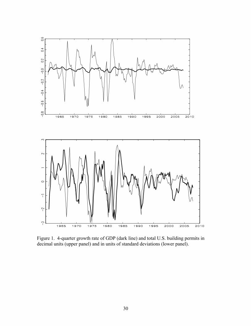
for both historical and contemporary reasons. From an historical perspective, as can be

seen in Figure 1 the issuance of building permits for new residential units has been

strongly procyclical, moving closely with overall growth in GDP but with much greater

volatility. Like GDP growth and other macroeconomic aggregates, building permits were

much more volatile before the mid-1980s than after the mid-1980s. In fact, the median

decline in the volatility of building permits is substantially greater than for other major

macroeconomic aggregates. From a contemporary perspective, building permits have

declined sharply recently, falling by approximately 30% nationally between 2006 and the

end of our sample, and the contraction in housing construction is a key real side-effect of

the decline in housing prices and the turbulence in financial markets during late 2007 into

2008. Because building permit data are available by state, there is potentially useful

information beyond that contained in the national aggregate plotted in Figure 1, but we

are unaware of any systematic empirical analysis of state-level building permit data.

2

In this paper, we build on Engle’s work and examine the co-evolution of state-

level building permits for residential units. Our broad aim is to provide new findings

concerning the link between housing construction, as measured by building permits, and

the decline in U.S. macroeconomic volatility since the mid-1980s known as the Great

Moderation. One hypothesis about the source of the Great Moderation in U.S. economic

activity is that developments in mortgage markets, such as the elimination of interest rate

ceilings and the bundling of mortgages to diversify the risk of holding a mortgage, led to

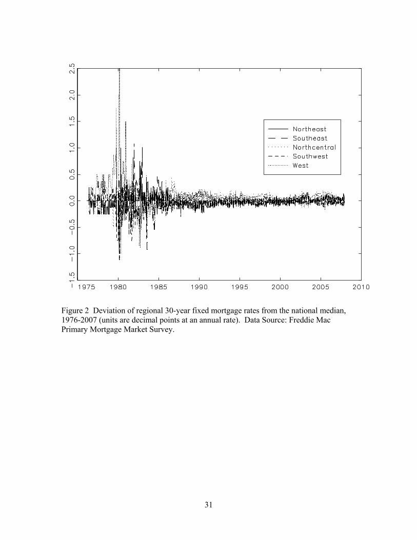
wider and less cyclically sensitive availability of housing credit. As can be seen in Figure

2, prior to the mid-1980s there were substantial regional differences in mortgage rates

across the U.S., however after approximately 1987 these differences disappeared,

suggesting that what had been regional mortgage markets become a single national

mortgage market. According to this theory, these changes in financial markets reduced

the cyclicality of mortgage credit, which in turn moderated the volatility of housing

construction and thus of overall employment.

This paper undertakes two specific tasks. The first task is to provide a new data

set on state-level monthly building permits and to provide descriptive statistics about

these data. This data set was put into electronic form from paper records provided by the

U.S. Bureau of the Census. These data allow us to characterize both the comovements

(spatial correlation) of permits across states and changes in volatility of state permits

from 1969 to the present.

The second task is to characterize the changes over time in the volatility of

building permits with an eye towards the Great Moderation. If financial market

developments were an important source of the Great Moderation, one would expect that

the volatility of building permits would exhibit a similar pattern across states, and

especially that any common or national component of building permits would exhibit a

decline in volatility consistent with the patterns documented in the literature on the Great

Moderation. Said differently, finding a lack of a substantial common component in

building permits along with substantial state-by-state differences in the evolution of

volatility would suggest that national-level changes in housing markets, such as the

secondary mortgage market, were not an important determinant of housing market

volatility.

3

The model we use to characterize the common and idiosyncratic aspects of

changes in state-level volatility is the dynamic factor model introduced by Geweke

(1977), modified to allow for stochastic volatility in the factors and the idiosyncratic

disturbances; we refer to this as the DFM-SV model. The filtered estimates of the state

variables implied by the DFM-SV model can be computed by Markov Chain Monte

Carlo (MCMC). The DFM-SV model is a multivariate extension of the univariate

unobserved components-stochastic volatility model in Stock and Watson (2007).

In the DFM-SV model, state-level building permits are a function of a single

national factor and one of five regional factors, plus a state-specific component. Thus

specification of the DFM-SV model requires determining which states belong in which

region. One approach would be to adopt the Department of Commerce’s definition of

U.S. regions, however as discussed in Crone (2005) that grouping of states was made for

administrative reasons and, while the groupings involved some economic considerations,

those considerations are now out of date. We therefore follow Crone (2005) by

estimating the regional composition using k-means cluster analysis. Our analysis differs

from Crone in three respects. First, we are interested in state building permits, while

Crone was interested in aggregate state-wide economic activity (measured by state

coincident indexes from Crone and Clayton Matthews (2005)). Second, we estimate the

clusters after extracting a single national factor whereas Crone (2005) estimated clusters

using business cycle components of the state-level data without first extracting a national

factor. Finally, because our measure of regions is whether states have housing markets

that behave similarly, there is no particular reason why states in regions must be

contiguous and we do not impose contiguity in the estimation of the regions.

The outline of the paper is as follows. The state-level building permits data set is

described in Section 2, along with initial descriptive statistics. The DFM-SV model is

introduced in Section 3. Section 4 contains the empirical results, and Section 5

concludes.

4

2. The State Building Permits Data Set

This section first describes the state housing start data set, then presents some

summary statistics and time series plots.

2.1 The Data

The underlying raw data are monthly observations on residential housing units

authorized by building permits by state, from 1969:1 – 2008:1. The data were obtained

from the U.S. Department of Commerce, Bureau of the Census, and are reported in the

monthly news release “New Residential Construction (Building Permits, Housing Starts,

and Housing Completions).” Data from 1988-present are available from Bureau of the

Census in electronic form.1 Data prior to 1988 are available in hard copy, which we

obtained from the Bureau of the Census. These data were converted into electronic form

by the Survey Research Center at Princeton University.

For the purpose of the building permits survey, a housing unit is defined as a new

housing unit intended for occupancy and maintained by occupants, thereby excluding

hotels, motels, group residential structures like college dorms, nursing homes, etc.

Mobile homes typically do not require a building permit so they are not counted as

authorized units.

Housing permit data are collected by a mail survey of selected permit-issuing

places (municipalities, counties, etc.), where the sample of places includes all the largest

permitting places and a random sample of the less active permitting places. In addition,

in states with few permitting places, all permitting places are included in the sample.

Currently the universe is approximately 20,000 permitting places, of which 9,000 are

sampled, and the survey results are used to estimate total monthly state permits. The

universe of permitting places has increased over time, from 13,000 at the beginning of the

sample to 20,000 since 1974.2

1 Monthly releases of building permits data and related documentation are provided at the Census Bureau Web site, http://www.census.gov/const/www/newresconstindex.html. 2 The number of permit issuing places in the universe sampled by date are: 1967-1971, 13,000; 1972-1977, 14,000; 1978-1983, 16,000; 1984-1993, 17,000; 1994-2003, 19,000; 2004-present, 20,000.

5

Precision of the survey estimates vary from state to state, depending on coverage.

As of January 2008, eight states have 100% coverage of permitting places so for these

states there is no sampling error. In an additional 34 states, the sampling standard error in

January 2008 was less than 5%. The states with the greatest sampling standard error are

Missouri (17%), Wyoming (17%), Ohio (13%), and Nebraska (12%).

In some locations, housing construction does not require a permit, and any

construction occurring in such a location is outside the universe of the survey. Currently

more than 98% of the U.S. population resides in permit-issuing areas. In some states,

however, the fraction of the population residing in a permit-issuing area is substantially

less; the states with the lowest percentages of population living within a permit-requiring

area are Arkansas (60%), Mississippi (65%), and Alabama (68%). In January 2008,

Arkansas had 100% of permitting places in the survey so there was no survey sampling

error, however the survey universe only covered 60% of Arkansas residents.3

The series analyzed in this paper is total residential housing units authorized by

building permits, which is the sum of authorized units in single-family and multiple-

family dwellings, where each apartment or town house within a multi-unit dwelling is

counted as a distinct unit.

The raw data are seasonally unadjusted and exhibit pronounced seasonality. Data

for each state was seasonally adjusted using the X12 program available from the Bureau

of the Census. Quarterly sums of the monthly data served as the basis for our analysis.

The quarterly data are from 1969:I through 2007:IV.4

2.2 Summary Statistics and Plots

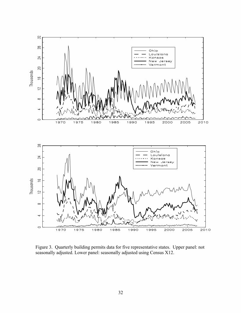
Quarterly data for five representative states, Vermont, New Jersey, Kansas,

Louisiana, and Ohio, are plotted in Figure 3 (upper panel). Three features are evident in

these plots. First, there is not a clear long-run overall trend in the number of permits

issued, and for these states the number of permits issued in 2007 is not substantially

different from the number issued in 1970. Second, the raw data are strongly seasonal, but

3 Additional information about the survey and the design is available at http://www.census.gov/const/www/newresconstdoc.html#reliabilitybp and http://www.census.gov/const/www/C40/sample.html 4 The raw data are available at http://www.princeton.edu/~mwatson.

6

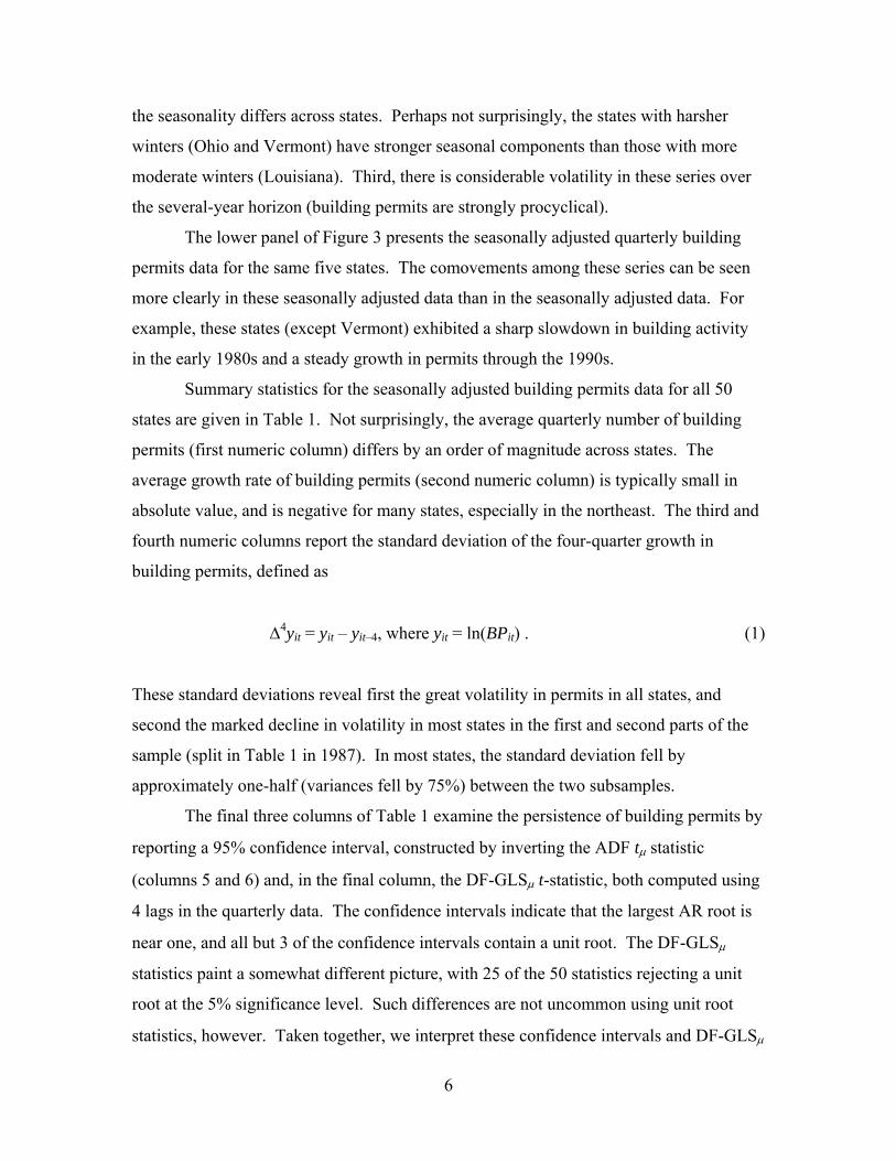
the seasonality differs across states. Perhaps not surprisingly, the states with harsher

winters (Ohio and Vermont) have stronger seasonal components than those with more

moderate winters (Louisiana). Third, there is considerable volatility in these series over

the several-year horizon (building permits are strongly procyclical).

The lower panel of Figure 3 presents the seasonally adjusted quarterly building

permits data for the same five states. The comovements among these series can be seen

more clearly in these seasonally adjusted data than in the seasonally adjusted data. For

example, these states (except Vermont) exhibited a sharp slowdown in building activity

in the early 1980s and a steady growth in permits through the 1990s.

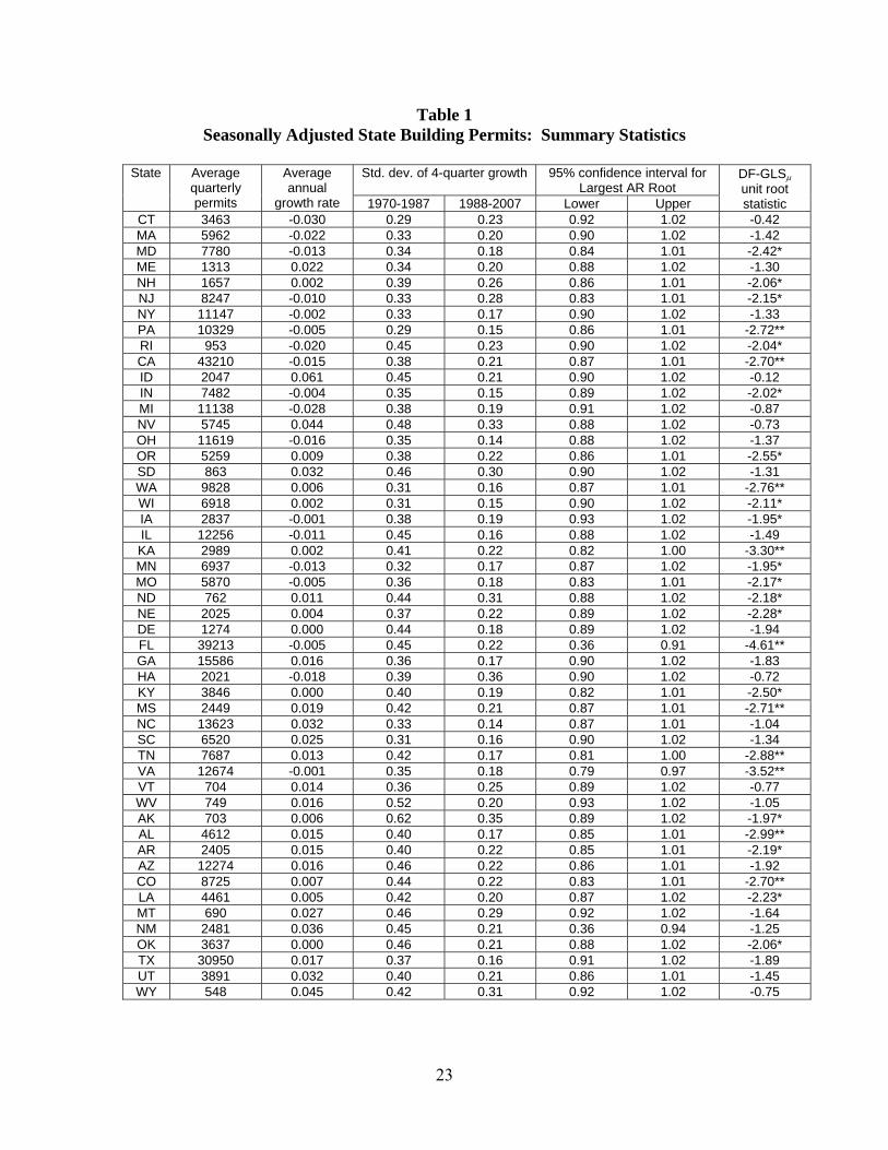
Summary statistics for the seasonally adjusted building permits data for all 50

states are given in Table 1. Not surprisingly, the average quarterly number of building

permits (first numeric column) differs by an order of magnitude across states. The

average growth rate of building permits (second numeric column) is typically small in

absolute value, and is negative for many states, especially in the northeast. The third and

fourth numeric columns report the standard deviation of the four-quarter growth in

building permits, defined as

Δ4yit = yit – yit–4, where yit = ln(BPit) . (1)

These standard deviations reveal first the great volatility in permits in all states, and

second the marked decline in volatility in most states in the first and second parts of the

sample (split in Table 1 in 1987). In most states, the standard deviation fell by

approximately one-half (variances fell by 75%) between the two subsamples.

The final three columns of Table 1 examine the persistence of building permits by

reporting a 95% confidence interval, constructed by inverting the ADF tμ statistic

(columns 5 and 6) and, in the final column, the DF-GLSμ t-statistic, both computed using

4 lags in the quarterly data. The confidence intervals indicate that the largest AR root is

near one, and all but 3 of the confidence intervals contain a unit root. The DF-GLSμ

statistics paint a somewhat different picture, with 25 of the 50 statistics rejecting a unit

root at the 5% significance level. Such differences are not uncommon using unit root

statistics, however. Taken together, we interpret these confidence intervals and DF-GLSμ

7

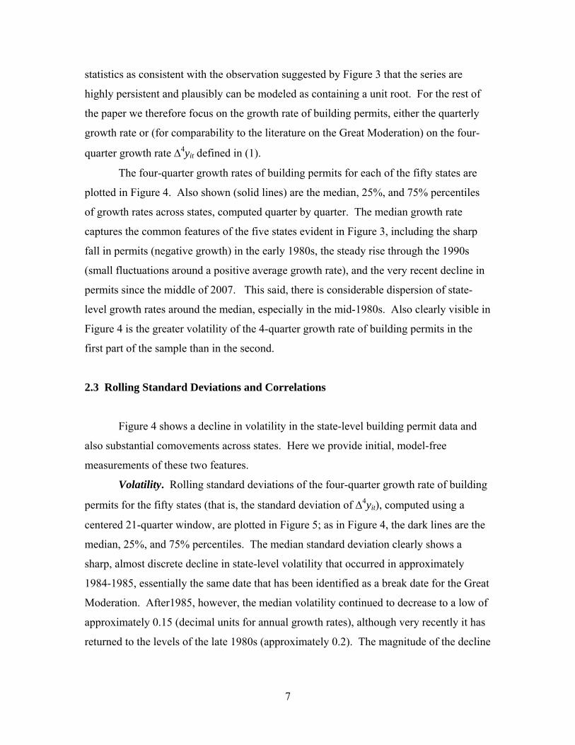
statistics as consistent with the observation suggested by Figure 3 that the series are

highly persistent and plausibly can be modeled as containing a unit root. For the rest of

the paper we therefore focus on the growth rate of building permits, either the quarterly

growth rate or (for comparability to the literature on the Great Moderation) on the four-

quarter growth rate Δ4yit defined in (1).

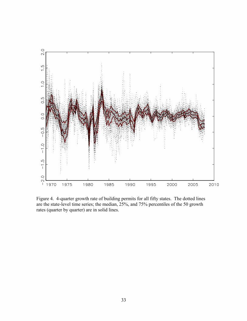
The four-quarter growth rates of building permits for each of the fifty states are

plotted in Figure 4. Also shown (solid lines) are the median, 25%, and 75% percentiles

of growth rates across states, computed quarter by quarter. The median growth rate

captures the common features of the five states evident in Figure 3, including the sharp

fall in permits (negative growth) in the early 1980s, the steady rise through the 1990s

(small fluctuations around a positive average growth rate), and the very recent decline in

permits since the middle of 2007. This said, there is considerable dispersion of state-

level growth rates around the median, especially in the mid-1980s. Also clearly visible in

Figure 4 is the greater volatility of the 4-quarter growth rate of building permits in the

first part of the sample than in the second.

2.3 Rolling Standard Deviations and Correlations

Figure 4 shows a decline in volatility in the state-level building permit data and

also substantial comovements across states. Here we provide initial, model-free

measurements of these two features.

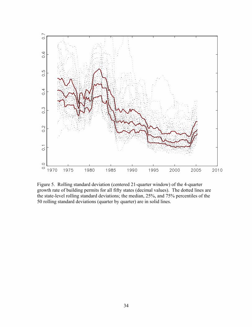
Volatility. Rolling standard deviations of the four-quarter growth rate of building

permits for the fifty states (that is, the standard deviation of Δ4yit), computed using a

centered 21-quarter window, are plotted in Figure 5; as in Figure 4, the dark lines are the

median, 25%, and 75% percentiles. The median standard deviation clearly shows a

sharp, almost discrete decline in state-level volatility that occurred in approximately

1984-1985, essentially the same date that has been identified as a break date for the Great

Moderation. After1985, however, the median volatility continued to decrease to a low of

approximately 0.15 (decimal units for annual growth rates), although very recently it has

returned to the levels of the late 1980s (approximately 0.2). The magnitude of the decline

8

is remarkable, from approximately 0.4 during the 1970s and 1980s to less than 0.2 on

average during the1990s and 2000’s.

Spatial correlation. There are, of course, many statistics available for

summarizing the comovements of two series, including cross correlations and spectral

measures such as coherence. In this application, a natural starting point is the correlation

between the four-quarter growth rates of two state series, computed over a rolling

window to allow for time variation. With a small number of series it is possible to

display the N(N–1)/2 pairs of cross-correlations, but this is not practical when N = 50.

We therefore draw on the spatial correlation literature for a single summary time series

that summarizes the possibly time-varying comovements among these 50 series.

Specifically, we use a measure based on Moran’s I, applied to a centered 21-quarter

rolling window. Let {Xi}, i = 1,…, N, be a spatial variable; then Moran’s I is

I = 1 1 1 1

2

1

( )( )

( )

N N N N

ij i j iji j i j

N

ii

w X X X X w

X X N

= = = =

=

− −

−

∑∑ ∑∑

∑ (2)

where wij is a spatial weight. Here, we are interested in the comovement over time across

all states (so wij = 1 for i ≠ j) as measured by the rolling cross-correlation in four-quarter

growth rates. Accordingly, the modified Moran’s I used here is

tI =

1

4 41 1

41

cov( , ) ( 1) / 2

var( )

N i

it jti j

N

iti

y y N N

y N

−

= =

=

Δ Δ −

Δ

∑∑

∑ (3)

where 4 4cov( , )it jty yΔ Δ = ( )( )10

4 4 4 410

121

t

is it js jts t

y y y y+

= −

Δ − Δ Δ −Δ∑ , 4var( )ityΔ =

( )10 2

4 410

121

t

is its t

y y+

= −

Δ − Δ∑ , 4 ityΔ = 10410

121

tiss t

y+

= −Δ∑ , and N = 50.

9

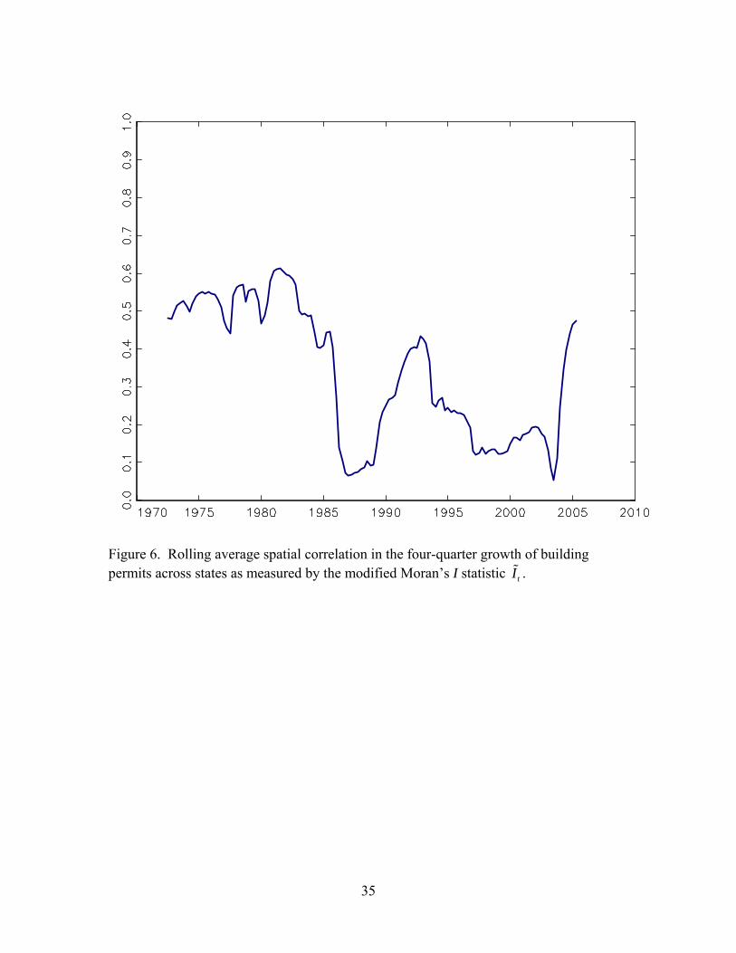
The time series tI is plotted in Figure 6. For the first half of the sample, the

spatial correlation was relatively large, approximately 0.5. Since 1985, however, the

spatial correlation has been substantially smaller, often less than 0.2 except in the early

1990s and in the very recent collapse of the housing market. Aside from these two

periods of national declines in housing construction, the spatial correlation in state

building permits seems to have fallen at approximately the same time as did their

volatility.

3. The DFM-SV Model

This section lays out the dynamic factor model with stochastic volatility (DFM-

SV) model and discusses the estimation of its parameters and the computation of the

filtered estimates of the state variables.

3.1 The Dynamic Factor Model with Stochastic Volatility

We examine the possibility that state-level building permits have a national

component, a regional component, and an idiosyncratic component. Specifically, we

model log building permits (yit) as following the dynamic factor model,

yit = αi + λiFt + 1

RN

ij jtj

Rγ=∑ + eit (4)

where the national factor Ft and the NR regional factors Rjt follow random walks and the

idiosyncratic disturbance eit follows an AR(1):

Ft = Ft−1 + ηt (5)

Rjt = Rjt−1 + υjt (6)

eit = ρieit−1 + εit, (7)

10

The disturbances ηt, υjt, and εit are independently distributed, where εit is i.i.d. N(0, 2εσ )

and the factor disturbances have stochastic volatility:

ηt = ση,tζη,t (8)

υjt = ,j tυσ ,j tυζ (9)

εit = ,i tεσ ,i tεζ (10)

ln 2,tησ = ln 2

, 1tησ − + νη,t (11)

ln 2,j tυσ = ln 2

, 1j tυσ − + ,j tυν (12)

ln 2,i tεσ = ln 2

, 1i tεσ − + ,i tεν (13)

where ζt = (ζη,t, 1 ,tυζ ,…, ,NR tυζ , 1 ,tεζ ,…, ,N tεζ )′ is i.i.d. N(0, 1 RN NI + + ), νt = (νη,t,

1 ,tυν ,…, ,NR tυν , 1 ,tεν ,…, ,N tεν )′ is i.i.d. N(0, φ 1 RN NI + + ), ζt and νt are independently

distributed, and φ is a scalar parameter.

The factors are identified by restrictions on the factor loadings. The national

factor enters all equations so {λi} is unrestricted. The regional factors are restricted to

load on only those variables in a region, so γij is nonzero if state i is in region j and is zero

otherwise. The scale of the factors is normalized setting λ′λ/N = 1 and γj′γj/NR,j = 1,

where λ = (λ1,…, λN)′, γj = (γ1j,…, γNj)′, and NR, is the number of state in region j.

The parameters of the model consist of {αi, λi, γij, ρi, 2εσ , φ}.5

3.2 Estimation and Filtering

Estimation of fixed model coefficients. Estimation was carried out using a two-

step process. In the first step, the parameters {αi, λi, γij, ρi}, i = 1, …, 50 were estimated

by Gaussian maximum likelihood in a model in which the values of 2ησ , 2

jυσ , and 2iε

σ are

allowed to break midway through the sample (1987:IV). The pre- and post-break values 5 The model (4)-(7) has tightly parameterized dynamics, and we have experimented with more loosely parameterized models that allow leads and lags of the factors to enter (4) and allow the factors to follow more general AR processes. The key empirical conclusions reported below were generally unaffected by these changes.

11

of the variances are modeled as unknown constants. This approximation greatly

simplifies the likelihood by eliminating the need to integrate out the stochastic volatility.

The likelihood is maximized using the EM algorithm described in Engle and Watson

(1983). The scale parameter φ (defined below equation (13)) was set equal to 0.04, a

value that we have used previously for univariate models (Stock and Watson (2007)).

Filtering. Conditioning on the values of {αi, λi, γij, ρi}, smoothed estimates of the

factors and variances E(Ft, Rjt, 2,tησ , 2

,j tυσ , 2,i tεσ | 50,

1, 1{ } Tiy τ ι τ= = ) were computed using Gibbs

sampling. Draws of { } { } { }5,50,5, 50, 2 2 2, , ,1, 11, 1 1, 1, 1

, | , , ,j i

TT Tt jt it t t ttj t j i t

F R y η υ εισ σ σ

= == = = = =

⎛ ⎞⎜ ⎟⎝ ⎠

were generated

from the relevant multivariate normal density using the algorithm in Carter and Kohn

(1994). Draws of { } { } { }5,50, 5,50,2 2 2

, , , 1, 1 1, 11, 1, 1, , | , ,

j i

T TTt t t it t jtt j tj i t

y F Rη υ ε ισ σ σ

= = = == = =

⎛ ⎞⎜ ⎟⎝ ⎠

were obtained using

a normal mixture approximation for the distribution of the logarithm of the 21χ random

variable (ln(ζ2)) and data augmentation as described in Shephard (1994) and Kim,

Shephard and Chibb (1998) (we used a bivariate normal mixture approximation). The

smoothed estimates and their standard deviations were approximated by sample averages

from 20,000 Gibbs draws (after discarding 1,000 initial draws). Repeating the simulations

using another set 20,000 independent resulted in estimates essentially indistinguishable

from the estimates obtained from the first set of draws.

4. Empirical Results

This section begins by describing the k-means method for estimation of the

housing market regions and discusses the results and the stability of the estimated regions

over time. Results are then given for the dynamic factor model, first using split-sample

methods without stochastic volatility then using the DFM-SV model.

4.1 Estimation of Housing Market Regions

In the DFM-SV model, regional variation is independent of national variation,

and any regional comovements would be most noticeable after removing the national

12

factor Ft. Accordingly, the housing market regions were estimated after removing a

single common component associated with the national factor. Our method follows

Crone (2005) by using k-means cluster analysis , except that we apply the k-means

procedure after subtracting the contribution of the national factor whereas Crone (2005)

applied it directly to the observed time series (in our notation, yit).

Specifically, the first step in estimating the regions used the single-factor model,

yit = αi + λiFt + uit (14)

Ft = Ft−1 + ηt (15)

uit = ρi1uit−1 + ρi2uit−2 + εit, (16)

where (ηt, ε1t,…, ε2t) is independently and distributed normal variables with mean zero

and constant variances. Note that in this specification, uit consists of the contribution of

the regional factors as well as the idiosyncratic term, see (4). The model (14) – (16) was

estimated by maximum likelihood, using as starting values least-squares estimates of the

coefficients using the first principal component as an estimator of Ft (Stock and Watson

(2002)). After subtracting out the common component, this produced the residual ˆitu =

yit – ˆiα – iλ tF .

The k-means method was then used to estimate the constituents of the clusters. In

general, let {Xi}, i = 1,…, N be a T-dimensional vector and let μj be the mean vector of Xi

if i is in cluster j. The k-means method solves,

{ , }minj jSμ ( ) ( )

1 j

k

i j i jj i S

X Xμ μ= ∈

′− −∑∑ (17)

where Sj is the set of indexes contained in cluster j. That is, the k-means method is the

least-squares solution to the problem of assigning entity i with data vector Xi to group j.6

6 In the context of the DFM under consideration, the model-consistent objective function would be to assign states to region so as to maximize the likelihood of the DFM. This is numerically infeasible, however, since each choice of index sets would require estimation of the DFM parameters.

13

We implemented the k-means cluster method using four-quarter changes in ˆitu ,

that is, with Xi = (Δ4 5ˆiu ,…,Δ4 ˆiTu )′. In principal (17) should be minimized over all

possible index sets Sj. With 50 states and more than two clusters, however, this is

computationally infeasible. We therefore used the following algorithm:

(i) An initial set of k clusters is assigned at random; call this S0.

(ii) The cluster sample means were computed for the grouping S0 yielding the k-

vector of means, 0μ

(iii) The distance from each Xi is computed to each element of 0μ and each state i is

reassigned to the cluster with the closest mean; call this grouping S1

(iv) The k cluster means 1μ are computed for the grouping S1, and steps (iii) and

(iv) are repeated until there are no switches or until the number of iterations

reaches 100.

This algorithm was repeated for multiple random starting values.

We undertook an initial cluster analysis to estimate the number of regions, in

which the foregoing algorithm was used with 20,000 random starting values. Moving

from 2 to 3 clusters reduced the value of the minimized objective function (17) by

approximately 10%, as did moving from 3 to 4 clusters. The improvements from 4 to 5,

and from 5 to 6, were less, and for 6 clusters the number of states was as few as five in

one of the clusters. Absent a statistical theory for estimating the number of clusters, and

lacking a persuasive reason for choosing 6 clusters, we therefore chose k = 5.

We then estimated the composition of these 5 regions using 400,000 random

starting values. We found that even after 200,000 starting values there were some

improvements in the objective function, however those improvements were very small

and the switches of states in regions involved were few. We then reestimated the regions

for the 1970-1987 and 1988-2007 subsamples, using 200,000 additional random starting

values and using the full-sample regional estimates as an additional starting value.

14

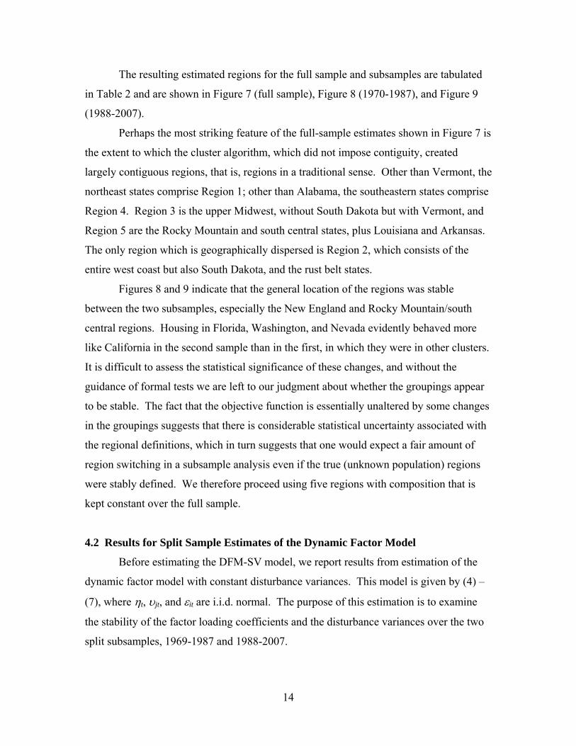
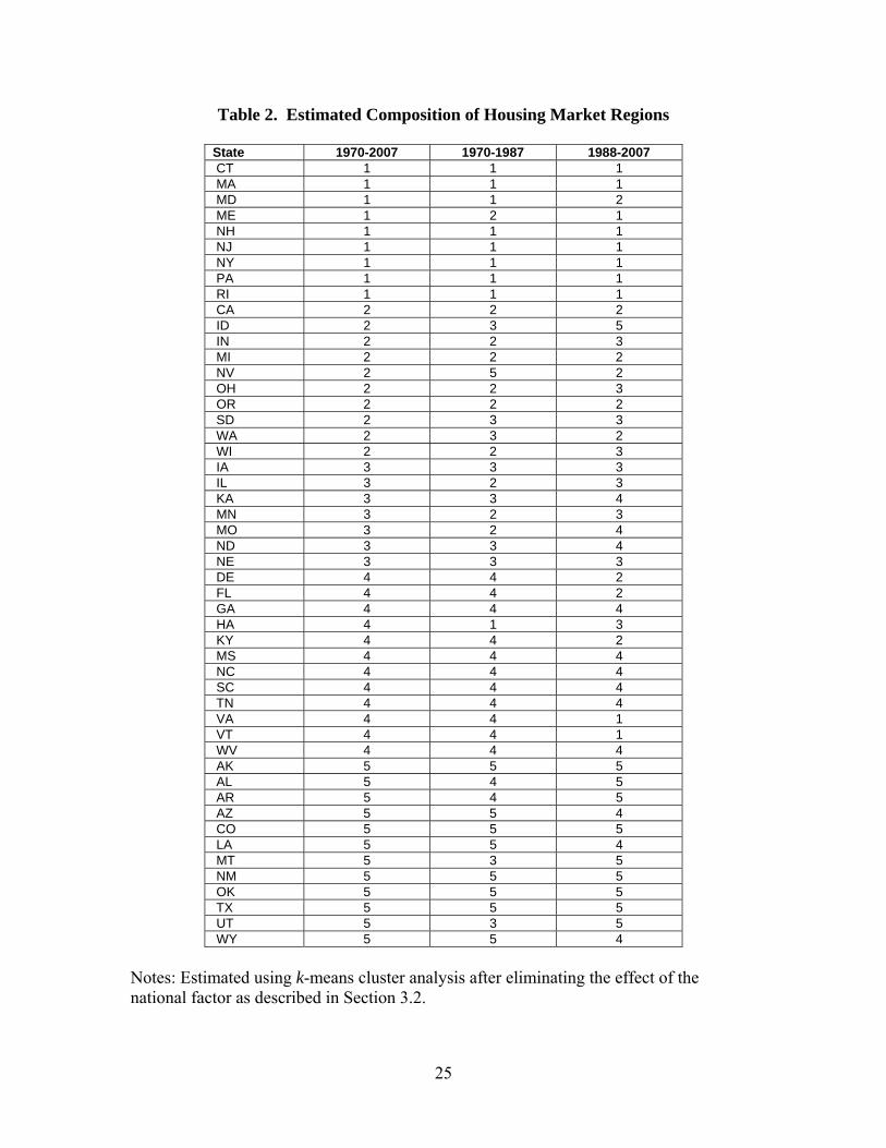
The resulting estimated regions for the full sample and subsamples are tabulated

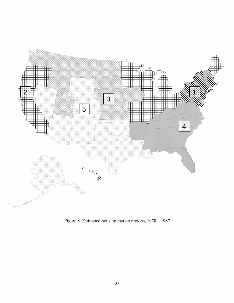
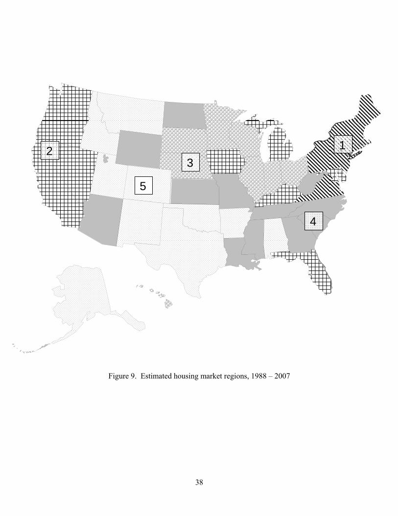
in Table 2 and are shown in Figure 7 (full sample), Figure 8 (1970-1987), and Figure 9

(1988-2007).

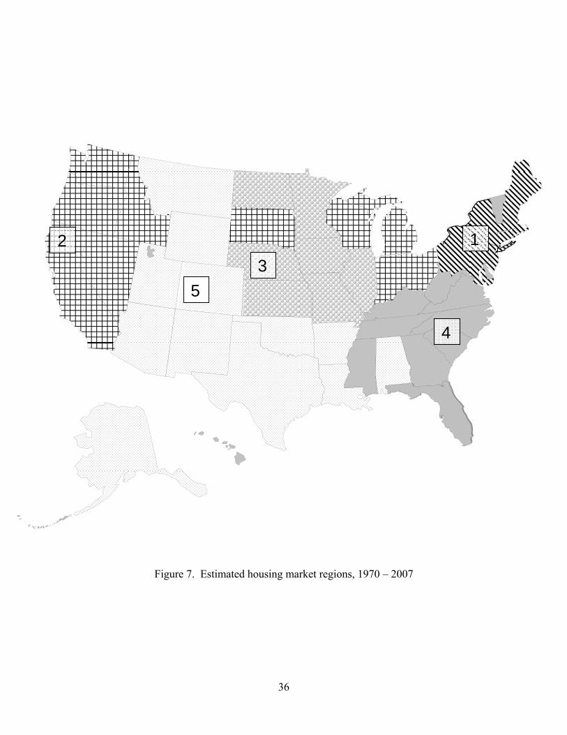
Perhaps the most striking feature of the full-sample estimates shown in Figure 7 is

the extent to which the cluster algorithm, which did not impose contiguity, created

largely contiguous regions, that is, regions in a traditional sense. Other than Vermont, the

northeast states comprise Region 1; other than Alabama, the southeastern states comprise

Region 4. Region 3 is the upper Midwest, without South Dakota but with Vermont, and

Region 5 are the Rocky Mountain and south central states, plus Louisiana and Arkansas.

The only region which is geographically dispersed is Region 2, which consists of the

entire west coast but also South Dakota, and the rust belt states.

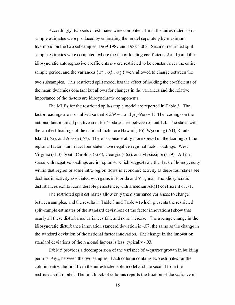
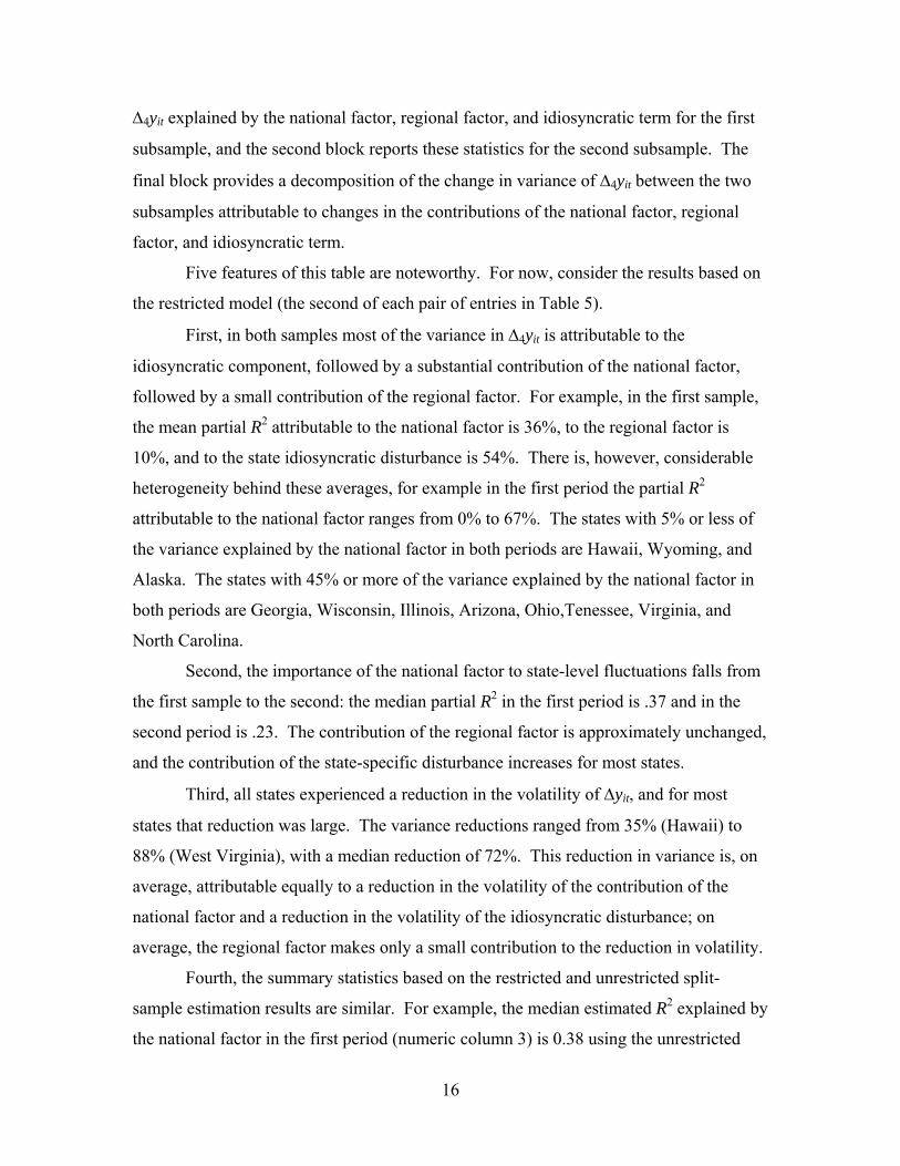
Figures 8 and 9 indicate that the general location of the regions was stable

between the two subsamples, especially the New England and Rocky Mountain/south

central regions. Housing in Florida, Washington, and Nevada evidently behaved more

like California in the second sample than in the first, in which they were in other clusters.

It is difficult to assess the statistical significance of these changes, and without the

guidance of formal tests we are left to our judgment about whether the groupings appear

to be stable. The fact that the objective function is essentially unaltered by some changes

in the groupings suggests that there is considerable statistical uncertainty associated with

the regional definitions, which in turn suggests that one would expect a fair amount of

region switching in a subsample analysis even if the true (unknown population) regions

were stably defined. We therefore proceed using five regions with composition that is

kept constant over the full sample.

4.2 Results for Split Sample Estimates of the Dynamic Factor Model

Before estimating the DFM-SV model, we report results from estimation of the

dynamic factor model with constant disturbance variances. This model is given by (4) –

(7), where ηt, υjt, and εit are i.i.d. normal. The purpose of this estimation is to examine

the stability of the factor loading coefficients and the disturbance variances over the two

split subsamples, 1969-1987 and 1988-2007.

15

Accordingly, two sets of estimates were computed. First, the unrestricted split-

sample estimates were produced by estimating the model separately by maximum

likelihood on the two subsamples, 1969-1987 and 1988-2008. Second, restricted split

sample estimates were computed, where the factor loading coefficients λ and γ and the

idiosyncratic autoregressive coefficients ρ were restricted to be constant over the entire

sample period, and the variances { 2ησ , 2

jνσ , 2iε

σ } were allowed to change between the

two subsamples. This restricted split model has the effect of holding the coefficients of

the mean dynamics constant but allows for changes in the variances and the relative

importance of the factors are idiosynchratic components.

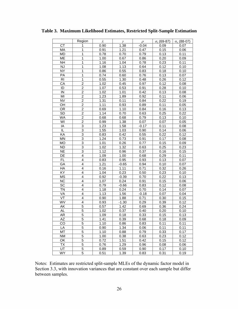
The MLEs for the restricted split-sample model are reported in Table 3. The

factor loadings are normalized so that λ′λ/N = 1 and γj′γj/NR,j = 1. The loadings on the

national factor are all positive and, for 44 states, are between .6 and 1.4. The states with

the smallest loadings of the national factor are Hawaii (.16), Wyoming (.51), Rhode

Island (.55), and Alaska (.57). There is considerably more spread on the loadings of the

regional factors, an in fact four states have negative regional factor loadings: West

Virginia (-1.3), South Carolina (-.66), Georgia (-.65), and Mississippi (-.39). All the

states with negative loadings are in region 4, which suggests a either lack of homogeneity

within that region or some intra-region flows in economic activity as these four states see

declines in activity associated with gains in Florida and Virginia. The idiosyncratic

disturbances exhibit considerable persistence, with a median AR(1) coefficient of .71.

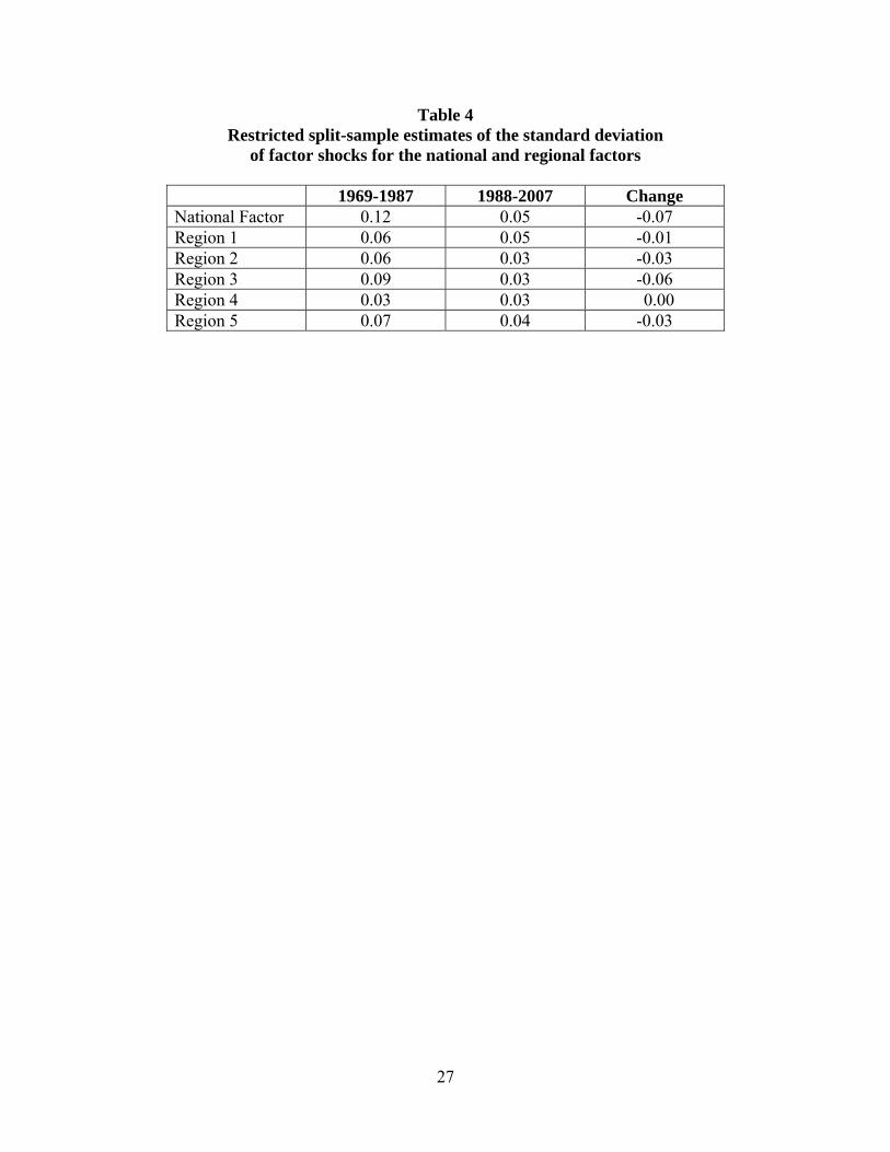
The restricted split estimates allow only the disturbance variances to change

between samples, and the results in Table 3 and Table 4 (which presents the restricted

split-sample estimates of the standard deviations of the factor innovations) show that

nearly all these disturbance variances fall, and none increase. The average change in the

idiosyncratic disturbance innovation standard deviation is -.07, the same as the change in

the standard deviation of the national factor innovation. The change in the innovation

standard deviations of the regional factors is less, typically -.03.

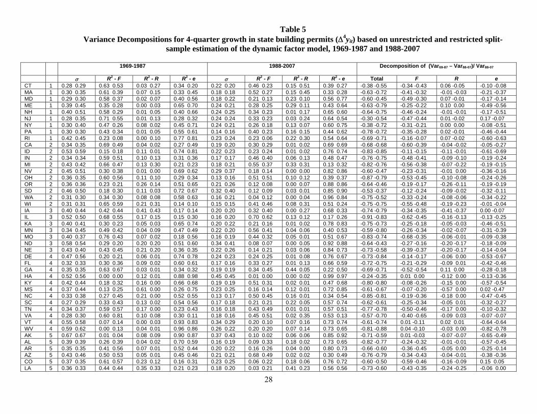
Table 5 provides a decomposition of the variance of 4-quarter growth in building

permits, Δ4yit, between the two samples. Each column contains two estimates for the

column entry, the first from the unrestricted split model and the second from the

restricted split model. The first block of columns reports the fraction of the variance of

16

Δ4yit explained by the national factor, regional factor, and idiosyncratic term for the first

subsample, and the second block reports these statistics for the second subsample. The

final block provides a decomposition of the change in variance of Δ4yit between the two

subsamples attributable to changes in the contributions of the national factor, regional

factor, and idiosyncratic term.

Five features of this table are noteworthy. For now, consider the results based on

the restricted model (the second of each pair of entries in Table 5).

First, in both samples most of the variance in Δ4yit is attributable to the

idiosyncratic component, followed by a substantial contribution of the national factor,

followed by a small contribution of the regional factor. For example, in the first sample,

the mean partial R2 attributable to the national factor is 36%, to the regional factor is

10%, and to the state idiosyncratic disturbance is 54%. There is, however, considerable

heterogeneity behind these averages, for example in the first period the partial R2

attributable to the national factor ranges from 0% to 67%. The states with 5% or less of

the variance explained by the national factor in both periods are Hawaii, Wyoming, and

Alaska. The states with 45% or more of the variance explained by the national factor in

both periods are Georgia, Wisconsin, Illinois, Arizona, Ohio,Tenessee, Virginia, and

North Carolina.

Second, the importance of the national factor to state-level fluctuations falls from

the first sample to the second: the median partial R2 in the first period is .37 and in the

second period is .23. The contribution of the regional factor is approximately unchanged,

and the contribution of the state-specific disturbance increases for most states.

Third, all states experienced a reduction in the volatility of Δyit, and for most

states that reduction was large. The variance reductions ranged from 35% (Hawaii) to

88% (West Virginia), with a median reduction of 72%. This reduction in variance is, on

average, attributable equally to a reduction in the volatility of the contribution of the

national factor and a reduction in the volatility of the idiosyncratic disturbance; on

average, the regional factor makes only a small contribution to the reduction in volatility.

Fourth, the summary statistics based on the restricted and unrestricted split-

sample estimation results are similar. For example, the median estimated R2 explained by

the national factor in the first period (numeric column 3) is 0.38 using the unrestricted

17

estimates and 0.36, using the restricted estimates. Similarly, the median fractional

change in the variance between the first and the second sample attributed to a reduction

in the contribution of the national factor (numeric column 11) is .31 for the unrestricted

estimates and .30 for the restricted estimates. These comparisons indicate that little is

lost, at least on average, by modeling the factor loadings and autoregressive coefficients

as constant across the two samples and allowing only the variances to change.7

Moreover, inspection of Table 5 reveals that the foregoing conclusions based on the

restricted estimates also follow from the unrestricted estimates.

4.3 Results for the DFM-SV Model

We now turn to the results based on the DFM-SV model. As discussed in Section

3.2, the parameters λ, γ, and ρ are fixed at the full-sample MLEs, and the filtered

estimates of the factors and their time-varying variances were computed numerically.

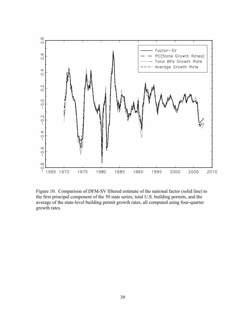
National and regional factors. The four-quarter growth of the estimated national

factor from the DFM-SV model, Δ4 tF , is plotted in Figure 10 along with three other

measures of national movements in building permits: the first principal component of the

50 series Δ4y1t,…, Δ4y50t,; the average state four-quarter growth rate, 5041

150 iti

y=Δ∑ , and

the 4-quarter growth rate of total national building permits, ln(BPt/BPt–4), where BPt = 50

1 itiBP

=∑ . The first principal component is an estimator of the four-quarter growth rate

of the national factor in a single-factor model (Stock and Watson (2002)), as is the

average of the state-level 4-quarter growth rates under the assumption that the average

population factor loading for the national factor is nonzero (Forni and Reichlin (1998)).

The fourth series plotted, the 4-quarter growth rate of national aggregate building

permits, does not have an interpretation as an estimate of the factor in a single-factor

version of the DFM specified in logarithms because the factor model is specified in

logarithms at the state level.

7 The restricted and unrestricted split-sample log-likelihoods differ by 280 points, with 194 additional parameters in the unrestricted model. However it would be heroic to rely on a chi-squared asymptotic distribution of the likelihood ratio statistic for inference with this many parameters.

18

As is clear from Figure 10, the three estimates of the factor (the DFM-SV

estimate, the first principal component, and the average of the state-level growth rates)

yields very nearly the same estimated 4-quarter growth of the national factor. These in

turn are close to the growth rate of national building permits, however there are some

discrepancies between the national permits and the estimates of the national factor,

particularly in 1974, 1990, and 2007. Like national building permits and consistent with

the split-sample analysis, the 4-quarter growth rate of the national factor shows a marked

reduction in volatility after 1985.

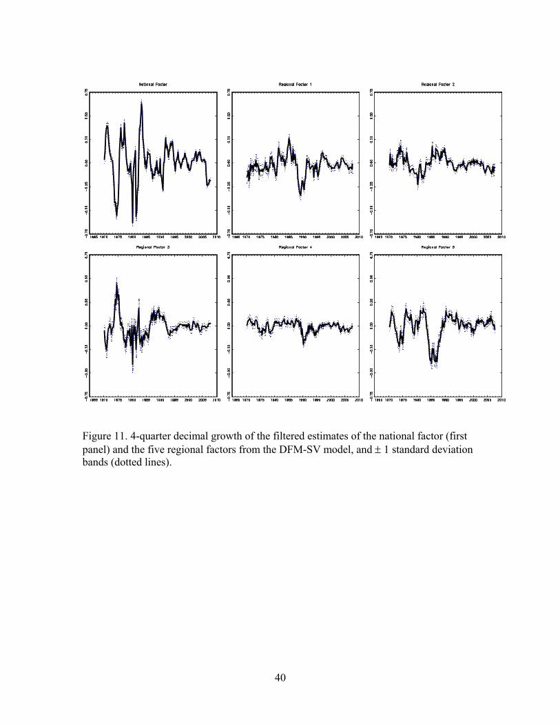
Figure 11 presents the four-quarter growth rates of the national and five regional

factors, along with ± 1 standard deviation bands, where the standard deviation bands

represent filtering uncertainty but not parameter estimation uncertainty (as discussed in

Section 3.2). The region factors show substantial variations across regions, for example

the housing slowdown in the mid-1980s in the south-central and the slowdown in the

late-1980s in the northeast are both visible in the regional factors, and these slowdowns

do not appear in other regions.

Figure 12 takes a closer look at the pattern of volatility in the national and

regional factors by reporting the estimated instantaneous standard deviation of the factor

innovations. The estimated volatility of the national factor falls markedly over the

middle of the sample, as does the volatility for region 3 (the upper Midwest). However

the pattern of volatility changes for regions other than 3 is more complicated; in fact,

there is evidence of a volatility peak in the 1980s in regions 1, 2, 4, and 5. This suggests

that the DFM-SV model attributes the common aspect of the decline in volatility of state

building permits over the sample to a decline in the volatility of the national factor.

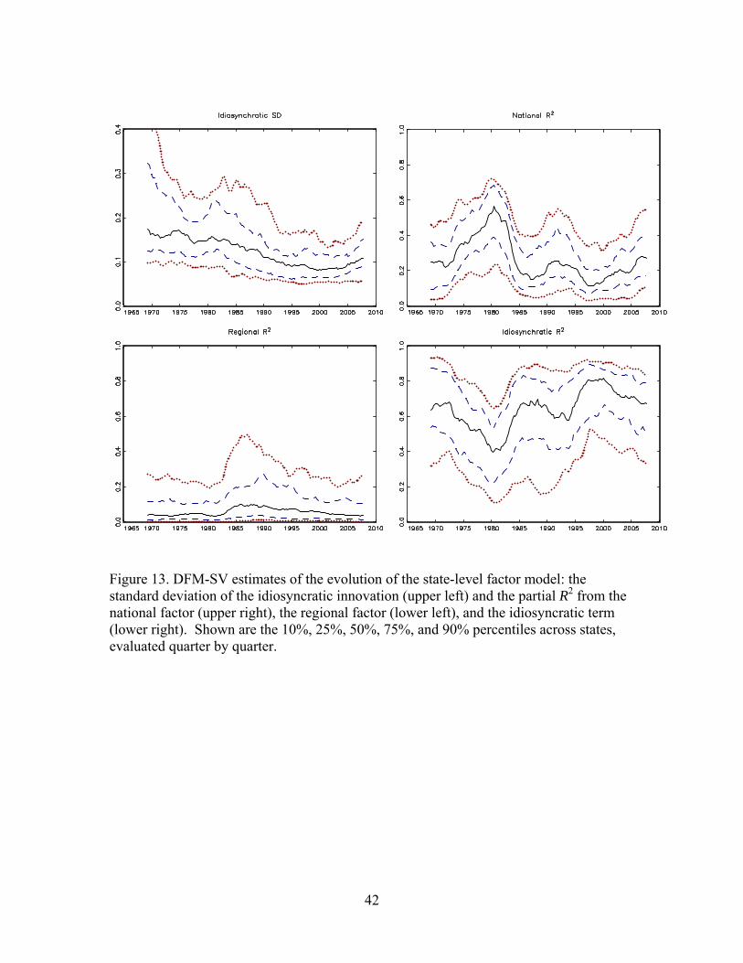
Figure 13 uses the DFM-SV estimates to compute statistics analogous to those

from the split sample analysis of Section 4.2, specifically, state-by-state instantaneous

estimates of the standard deviation of the innovation to the idiosyncratic disturbance and

the partial R2 attributable to the national and regional factors and to the idiosyncratic

disturbance. The conclusions are consistent with those reached by the examination of the

split-sample results in Table 5. Specifically, for a typical state the fraction of the state-

level variance of Δ4yit explained by the national factor has declined over time, the fraction

attributable to the idiosyncratic disturbance has increased, and the fraction attributable to

19

the regional factor has remained approximately constant. In addition, the volatility of the

idiosyncratic disturbance has decreased over time.

This said, the patterns in Figure 13 suggest some nuances that the split-sample

analysis masks. Notably, the idiosyncratic standard deviation declines at a nearly

constant rate over this period, and does not appear to be well characterized as having a

single break. The volatility of the regional factor does not appear to be constant, and

instead increases substantially for many states in the 1980s. Also, the importance of the

national factor has fluctuated over time: it was greatest during the recessions of the late

70s/early 80s, but in the early 1970s the contribution of the national factor was essentially

the same as in 2007. For this partial R2 associated with the national factor, the pattern

that emerges is less one of a sharp break than of a slow evolution.

5. Discussion and Conclusions

The empirical results in Section 4 suggest five main findings that bear on the

issues, laid out in the introduction, about the relationship between state-level volatility in

housing construction and the Great Moderation in overall U.S. economic activity.

First, there has been a large reduction in the volatility of state-level housing

construction, with the state-level standard deviation of the four-quarter growth in building

permits falling by between 35% and 88% from the period 1970-1987 to the period 1988-

2007, with a median decline of 72%.

Second, according to the estimates from the state building permit DFM-SV

model, there was a substantial decline in the volatility of the national factor, and this

decline occurred sharply in the mid-1980s. On average, this reduction in the volatility of

the national factor accounted for one-half of the reduction in the variance of four-quarter

growth in state building permits.

Third, there is evidence of regional organization of housing markets and,

intriguingly, the cluster analytic methods we used to estimate the composition of the

regions resulted in five conventionally identifiable regions – the northeast, southeast,

upper midwest, Rockies, and west coast – even though no constraints were imposed

requiring the estimated regions to be contiguous. The regional factors, however, explain

20

only a modest amount of state-level fluctuations in building permits, and the regional

factors show no systematic decline in volatility; if anything, they exhibit a peak in

volatility in the mid-1980s.

Fourth, there has been a steady decline in the volatility of the idiosyncratic

component of state building permits over the period 1970-2007. The smooth pattern of

this decline is different than that for macroeconomic aggregates or for the national factor,

which exhibit striking declines in volatility in the mid-1980s.

Taken together, these findings are consistent with the view, outlined in the

introduction, that the development of financial markets played an important role in the

Great Moderation: less cyclically sensitive access to credit coincided with a decline in

the volatility of the national factor in building permits, which in turn led to declines in the

volatility of state housing construction. The timing of the decline in the volatility of the

national housing factor coincides with the harmonization of mortgage rates across regions

in Figure 2, the mid-1980s.

This said, the evidence here is reduced-form, and the moderation of national

factor presumably reflects many influences, including moderation in the volatility of

income. Sorting out these multiple influences would require augmenting the state

building permits set developed here with other data, such as state-level incomes.

21

References

Carter, C.K. and R. Kohn (1994), “On Gibbs Sampling for State Space Models,”

Biometrika, 81, 541-553.

Crone, T.M. (2005), “An Alternative Definition of Economic Regions in the United

States based on Similarities in State Business Cycles,” The Review of Economics

and Statistics 87, 617-626.

Crone, T.M. and Alan Clayton-Matthews (2005), “Consistent Economic Indexes for the

50 States,” The Review of Economics and Statistics 87, 593-603.

Engle, R.F. (1978), “Estimating structural models of seasonality,” in Seasonal Analysis of

Economic Time Series, ed. A. Zellner (U.S. Department of Commerce, Bureau of

Census).

Engle, R.F. (1982), “Autoregressive Conditional Heteroskedasticity With Estimates of

the Variance of U.K. Inflation,” Econometrica 50: 987-1008.

Engle, R.F. and M.W. Watson (1981), “A One-Factor Multivariate Time Series Model of

Metropolitan Wage Rates,” Journal of the American Statistical Association 76,

No. 376, 774-781.

Engle, R.F. and M.W. Watson (1983), “Alternative Algorithms for Estimation of

Dynamic MIMIC, Factor, and Time Varying Coefficient Regression Models,”

Journal of Econometrics, Vol. 23, pp. 385-400.

Engle, R.F., D.M. Lilien, and M.W. Watson (1985), “A DYMIMIC Model of Housing

Price Determination,” Journal of Econometrics, Vol. 28, pp. 307-326.

Forni, M., and L. Reichlin (1998), “Let’s get real: a dynamic factor analytical approach to

disaggregated business cycle,” Review of Economic Studies 65:453-474.

Geweke, J. (1977), “The Dynamic Factor Analysis of Economic Time Series”, in: D.J.

Aigner and A.S. Goldberger, eds., Latent Variables in Socio-Economic Models,

North-Holland: Amsterdam.

Kim, S., N. Shephard and S. Chib (1998), “Stochastic Volatility: Likelihood Inference

and Comparison with ARCH Models,” Review of Economic Studies, 65, 361-393.

Shephard, N.H, (1994), “Partial non-Gaussian state space,” Biometrika 81, 115–131.

22

Stock, J.H., and M.W. Watson (2002), “Forecasting Using Principal Components from a

Large Number of Predictors,” Journal of the American Statistical Association

97:1167–1179.

Stock, J.H., and M.W. Watson (2007), “Why Has U.S. Inflation Become Harder to

Forecast?” Journal of Money, Credit, and Banking 39, 3-34.

23

Table 1 Seasonally Adjusted State Building Permits: Summary Statistics

State Average

quarterly permits

Average annual

growth rate

Std. dev. of 4-quarter growth

95% confidence interval for Largest AR Root

DF-GLSμ unit root statistic 1970-1987 1988-2007 Lower Upper

CT 3463 -0.030 0.29 0.23 0.92 1.02 -0.42 MA 5962 -0.022 0.33 0.20 0.90 1.02 -1.42 MD 7780 -0.013 0.34 0.18 0.84 1.01 -2.42* ME 1313 0.022 0.34 0.20 0.88 1.02 -1.30 NH 1657 0.002 0.39 0.26 0.86 1.01 -2.06* NJ 8247 -0.010 0.33 0.28 0.83 1.01 -2.15* NY 11147 -0.002 0.33 0.17 0.90 1.02 -1.33 PA 10329 -0.005 0.29 0.15 0.86 1.01 -2.72** RI 953 -0.020 0.45 0.23 0.90 1.02 -2.04* CA 43210 -0.015 0.38 0.21 0.87 1.01 -2.70** ID 2047 0.061 0.45 0.21 0.90 1.02 -0.12 IN 7482 -0.004 0.35 0.15 0.89 1.02 -2.02* MI 11138 -0.028 0.38 0.19 0.91 1.02 -0.87 NV 5745 0.044 0.48 0.33 0.88 1.02 -0.73 OH 11619 -0.016 0.35 0.14 0.88 1.02 -1.37 OR 5259 0.009 0.38 0.22 0.86 1.01 -2.55* SD 863 0.032 0.46 0.30 0.90 1.02 -1.31 WA 9828 0.006 0.31 0.16 0.87 1.01 -2.76** WI 6918 0.002 0.31 0.15 0.90 1.02 -2.11* IA 2837 -0.001 0.38 0.19 0.93 1.02 -1.95* IL 12256 -0.011 0.45 0.16 0.88 1.02 -1.49 KA 2989 0.002 0.41 0.22 0.82 1.00 -3.30** MN 6937 -0.013 0.32 0.17 0.87 1.02 -1.95* MO 5870 -0.005 0.36 0.18 0.83 1.01 -2.17* ND 762 0.011 0.44 0.31 0.88 1.02 -2.18* NE 2025 0.004 0.37 0.22 0.89 1.02 -2.28* DE 1274 0.000 0.44 0.18 0.89 1.02 -1.94 FL 39213 -0.005 0.45 0.22 0.36 0.91 -4.61** GA 15586 0.016 0.36 0.17 0.90 1.02 -1.83 HA 2021 -0.018 0.39 0.36 0.90 1.02 -0.72 KY 3846 0.000 0.40 0.19 0.82 1.01 -2.50* MS 2449 0.019 0.42 0.21 0.87 1.01 -2.71** NC 13623 0.032 0.33 0.14 0.87 1.01 -1.04 SC 6520 0.025 0.31 0.16 0.90 1.02 -1.34 TN 7687 0.013 0.42 0.17 0.81 1.00 -2.88** VA 12674 -0.001 0.35 0.18 0.79 0.97 -3.52** VT 704 0.014 0.36 0.25 0.89 1.02 -0.77 WV 749 0.016 0.52 0.20 0.93 1.02 -1.05 AK 703 0.006 0.62 0.35 0.89 1.02 -1.97* AL 4612 0.015 0.40 0.17 0.85 1.01 -2.99** AR 2405 0.015 0.40 0.22 0.85 1.01 -2.19* AZ 12274 0.016 0.46 0.22 0.86 1.01 -1.92 CO 8725 0.007 0.44 0.22 0.83 1.01 -2.70** LA 4461 0.005 0.42 0.20 0.87 1.02 -2.23* MT 690 0.027 0.46 0.29 0.92 1.02 -1.64 NM 2481 0.036 0.45 0.21 0.36 0.94 -1.25 OK 3637 0.000 0.46 0.21 0.88 1.02 -2.06* TX 30950 0.017 0.37 0.16 0.91 1.02 -1.89 UT 3891 0.032 0.40 0.21 0.86 1.01 -1.45 WY 548 0.045 0.42 0.31 0.92 1.02 -0.75

24

Notes to Table 1: The units for the first numeric column are units permitted per quarter. The units for columns 2-4 are decimal annual growth rates. The 95% confidence interval for the largest autoregressive root in column 5 is computed by inverting the ADFμ t-statistic, computed using 4 lags. The final column reports the DF-GLSμ t-statistic, also computed using 4 lags. The DF-GLSμ t-statistic rejects the unit root at the: *5% or **1% significance level. The full quarterly data set spans 1969Q1 – 2007Q4.

25

Table 2. Estimated Composition of Housing Market Regions

State 1970-2007 1970-1987 1988-2007 CT 1 1 1 MA 1 1 1 MD 1 1 2 ME 1 2 1 NH 1 1 1 NJ 1 1 1 NY 1 1 1 PA 1 1 1 RI 1 1 1 CA 2 2 2 ID 2 3 5 IN 2 2 3 MI 2 2 2 NV 2 5 2 OH 2 2 3 OR 2 2 2 SD 2 3 3 WA 2 3 2 WI 2 2 3 IA 3 3 3 IL 3 2 3 KA 3 3 4 MN 3 2 3 MO 3 2 4 ND 3 3 4 NE 3 3 3 DE 4 4 2 FL 4 4 2 GA 4 4 4 HA 4 1 3 KY 4 4 2 MS 4 4 4 NC 4 4 4 SC 4 4 4 TN 4 4 4 VA 4 4 1 VT 4 4 1 WV 4 4 4 AK 5 5 5 AL 5 4 5 AR 5 4 5 AZ 5 5 4 CO 5 5 5 LA 5 5 4 MT 5 3 5 NM 5 5 5 OK 5 5 5 TX 5 5 5 UT 5 3 5 WY 5 5 4

Notes: Estimated using k-means cluster analysis after eliminating the effect of the national factor as described in Section 3.2.

26

Table 3. Maximum Likelihood Estimates, Restricted Split-Sample Estimation

Region λ γ ρ σε (69-87) σε (88-07) CT 1 0.90 1.38 -0.04 0.09 0.07 MA 1 0.91 1.21 0.47 0.15 0.06 MD 1 0.78 0.70 0.79 0.13 0.11 ME 1 1.00 0.67 0.86 0.20 0.09 NH 1 1.16 1.04 0.78 0.23 0.11 NJ 1 1.08 1.13 0.64 0.12 0.10 NY 1 0.86 0.55 0.83 0.18 0.10 PA 1 0.74 0.60 0.76 0.13 0.07 RI 1 0.55 1.30 0.48 0.26 0.12 CA 2 1.02 0.45 0.97 0.12 0.08 ID 2 1.07 0.53 0.91 0.28 0.10 IN 2 1.02 1.01 0.42 0.13 0.08 MI 2 1.23 1.89 0.92 0.11 0.06 NV 2 1.31 0.11 0.84 0.22 0.19 OH 2 1.11 0.93 0.89 0.11 0.05 OR 2 0.69 1.10 0.84 0.16 0.13 SD 2 1.14 0.70 0.63 0.25 0.22 WA 2 0.68 0.68 0.79 0.13 0.10 WI 2 0.99 1.38 0.07 0.07 0.05 IA 3 1.23 1.58 -0.17 0.11 0.08 IL 3 1.55 1.03 0.90 0.14 0.06 KA 3 0.83 0.42 0.55 0.22 0.12 MN 3 1.24 0.73 0.91 0.17 0.08 MO 3 1.01 0.26 0.77 0.15 0.09 ND 3 1.02 1.32 0.63 0.25 0.23 NE 3 1.12 0.96 0.37 0.16 0.15 DE 4 1.09 1.00 0.68 0.29 0.11 FL 4 0.83 0.95 0.93 0.13 0.07 GA 4 1.21 -0.65 0.94 0.10 0.07 HA 4 0.16 1.11 0.71 0.32 0.26 KY 4 1.04 0.23 0.50 0.23 0.10 MS 4 0.92 -0.39 0.70 0.22 0.13 NC 4 1.07 0.24 0.91 0.15 0.06 SC 4 0.79 -0.66 0.83 0.12 0.08 TN 4 1.18 0.24 0.70 0.14 0.07 VA 4 1.13 1.56 -0.18 0.07 0.04 VT 4 0.90 1.88 0.71 0.30 0.15 WV 4 0.93 -1.30 0.29 0.39 0.12 AK 5 0.57 1.42 0.69 0.36 0.24 AL 5 1.02 0.37 0.40 0.20 0.10 AR 5 1.09 0.18 0.33 0.15 0.13 AZ 5 1.41 0.39 0.68 0.18 0.09 CO 5 1.10 0.86 0.83 0.11 0.11 LA 5 0.90 1.34 0.06 0.11 0.11 MT 5 1.10 0.88 0.79 0.33 0.17 NM 5 1.00 0.38 0.63 0.23 0.12 OK 5 0.72 1.51 0.42 0.15 0.12 TX 5 0.76 1.29 0.96 0.08 0.06 UT 5 0.89 0.59 0.90 0.17 0.10 WY 5 0.51 1.39 0.83 0.31 0.19

Notes: Estimates are restricted split-sample MLEs of the dynamic factor model in Section 3.3, with innovation variances that are constant over each sample but differ between samples.

27

Table 4 Restricted split-sample estimates of the standard deviation

of factor shocks for the national and regional factors

1969-1987 1988-2007 Change National Factor 0.12 0.05 -0.07 Region 1 0.06 0.05 -0.01 Region 2 0.06 0.03 -0.03 Region 3 0.09 0.03 -0.06 Region 4 0.03 0.03 0.00 Region 5 0.07 0.04 -0.03

28

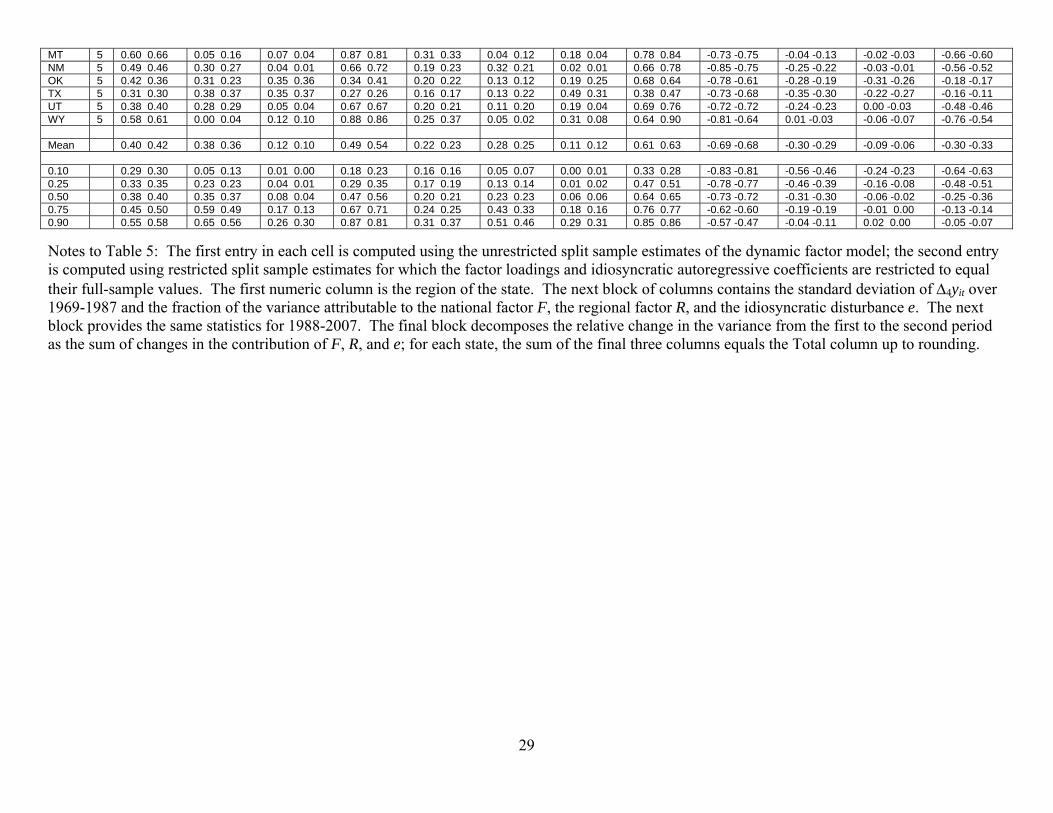
Table 5 Variance Decompositions for 4-quarter growth in state building permits (Δ4yit) based on unrestricted and restricted split-

sample estimation of the dynamic factor model, 1969-1987 and 1988-2007

1969-1987 1988-2007 Decomposition of (Var69-87 – Var88-07)/ Var88-07

σ R2 - F R2 - R R2 - e σ R2 - F R2 - R R2 - e Total F R e CT 1 0.28 0.29 0.63 0.53 0.03 0.27 0.34 0.20 0.22 0.20 0.46 0.23 0.15 0.51 0.39 0.27 -0.38 -0.55 -0.34 -0.43 0.06 -0.05 -0.10 -0.08 MA 1 0.30 0.35 0.61 0.39 0.07 0.15 0.33 0.45 0.18 0.18 0.52 0.27 0.15 0.45 0.33 0.28 -0.63 -0.72 -0.41 -0.32 -0.01 -0.03 -0.21 -0.37 MD 1 0.29 0.30 0.58 0.37 0.02 0.07 0.40 0.56 0.18 0.22 0.21 0.13 0.23 0.10 0.56 0.77 -0.60 -0.45 -0.49 -0.30 0.07 -0.01 -0.17 -0.14 ME 1 0.39 0.45 0.35 0.28 0.00 0.03 0.65 0.70 0.24 0.21 0.28 0.25 0.29 0.11 0.43 0.64 -0.63 -0.79 -0.25 -0.22 0.10 0.00 -0.49 -0.56 NH 1 0.40 0.51 0.58 0.29 0.01 0.05 0.40 0.66 0.24 0.25 0.34 0.23 0.01 0.17 0.65 0.60 -0.64 -0.75 -0.46 -0.24 -0.01 -0.01 -0.17 -0.51 NJ 1 0.28 0.35 0.71 0.55 0.01 0.13 0.28 0.32 0.24 0.24 0.33 0.23 0.03 0.24 0.64 0.54 -0.30 -0.54 -0.47 -0.44 0.01 -0.02 0.17 -0.07 NY 1 0.30 0.40 0.47 0.26 0.08 0.02 0.45 0.71 0.24 0.21 0.26 0.18 0.13 0.07 0.60 0.75 -0.38 -0.72 -0.31 -0.21 0.00 0.00 -0.08 -0.51 PA 1 0.30 0.30 0.43 0.34 0.01 0.05 0.55 0.61 0.14 0.16 0.40 0.23 0.16 0.15 0.44 0.62 -0.78 -0.72 -0.35 -0.28 0.02 -0.01 -0.46 -0.44 RI 1 0.42 0.45 0.23 0.08 0.00 0.10 0.77 0.81 0.23 0.24 0.23 0.06 0.22 0.30 0.54 0.64 -0.69 -0.71 -0.16 -0.07 0.07 -0.02 -0.60 -0.63 CA 2 0.34 0.35 0.69 0.49 0.04 0.02 0.27 0.49 0.19 0.20 0.30 0.29 0.01 0.02 0.69 0.69 -0.68 -0.68 -0.60 -0.39 -0.04 -0.02 -0.05 -0.27 ID 2 0.53 0.59 0.15 0.18 0.11 0.01 0.74 0.81 0.22 0.23 0.23 0.24 0.01 0.02 0.76 0.74 -0.83 -0.85 -0.11 -0.15 -0.11 -0.01 -0.61 -0.69 IN 2 0.34 0.34 0.59 0.51 0.10 0.13 0.31 0.36 0.17 0.17 0.46 0.40 0.06 0.13 0.48 0.47 -0.76 -0.75 -0.48 -0.41 -0.09 -0.10 -0.19 -0.24 MI 2 0.43 0.42 0.66 0.47 0.13 0.30 0.21 0.23 0.18 0.21 0.55 0.37 0.33 0.31 0.13 0.32 -0.82 -0.76 -0.56 -0.38 -0.07 -0.22 -0.19 -0.15 NV 2 0.45 0.51 0.30 0.38 0.01 0.00 0.69 0.62 0.29 0.37 0.18 0.14 0.00 0.00 0.82 0.86 -0.60 -0.47 -0.23 -0.31 -0.01 0.00 -0.36 -0.16 OH 2 0.36 0.35 0.60 0.56 0.11 0.10 0.29 0.34 0.13 0.16 0.51 0.51 0.10 0.12 0.39 0.37 -0.87 -0.79 -0.53 -0.45 -0.10 -0.08 -0.24 -0.26 OR 2 0.36 0.36 0.23 0.21 0.26 0.14 0.51 0.65 0.21 0.26 0.12 0.08 0.00 0.07 0.88 0.86 -0.64 -0.46 -0.19 -0.17 -0.26 -0.11 -0.19 -0.19 SD 2 0.46 0.50 0.18 0.30 0.11 0.03 0.72 0.67 0.32 0.40 0.12 0.09 0.03 0.01 0.85 0.90 -0.53 -0.37 -0.12 -0.24 -0.09 -0.02 -0.32 -0.11 WA 2 0.31 0.30 0.34 0.30 0.08 0.08 0.58 0.63 0.16 0.21 0.04 0.12 0.00 0.04 0.96 0.84 -0.75 -0.52 -0.33 -0.24 -0.08 -0.06 -0.34 -0.22 WI 2 0.31 0.31 0.65 0.59 0.21 0.31 0.14 0.10 0.15 0.15 0.41 0.46 0.08 0.31 0.51 0.24 -0.75 -0.75 -0.55 -0.48 -0.19 -0.23 -0.01 -0.04 IA 3 0.40 0.44 0.42 0.44 0.41 0.43 0.17 0.14 0.20 0.20 0.32 0.40 0.00 0.27 0.68 0.33 -0.74 -0.79 -0.34 -0.35 -0.41 -0.37 0.00 -0.07 IL 3 0.52 0.50 0.68 0.55 0.17 0.15 0.15 0.30 0.16 0.20 0.70 0.62 0.13 0.12 0.17 0.26 -0.91 -0.83 -0.62 -0.45 -0.16 -0.13 -0.13 -0.25 KA 3 0.40 0.41 0.30 0.23 0.05 0.03 0.65 0.74 0.20 0.22 0.21 0.16 0.01 0.02 0.78 0.83 -0.75 -0.73 -0.25 -0.18 -0.05 -0.03 -0.46 -0.51 MN 3 0.34 0.45 0.49 0.42 0.04 0.09 0.47 0.49 0.22 0.20 0.56 0.41 0.04 0.06 0.40 0.53 -0.59 -0.80 -0.26 -0.34 -0.02 -0.07 -0.31 -0.39 MO 3 0.40 0.37 0.76 0.43 0.07 0.02 0.18 0.56 0.16 0.19 0.44 0.32 0.05 0.01 0.51 0.67 -0.83 -0.74 -0.68 -0.35 -0.06 -0.01 -0.09 -0.38 ND 3 0.58 0.54 0.29 0.20 0.20 0.20 0.51 0.60 0.34 0.41 0.08 0.07 0.00 0.05 0.92 0.88 -0.64 -0.43 -0.27 -0.16 -0.20 -0.17 -0.18 -0.09 NE 3 0.43 0.40 0.43 0.45 0.21 0.20 0.36 0.35 0.22 0.26 0.14 0.21 0.03 0.06 0.84 0.73 -0.73 -0.58 -0.39 -0.37 -0.20 -0.17 -0.14 -0.04 DE 4 0.47 0.56 0.20 0.21 0.06 0.01 0.74 0.78 0.24 0.23 0.24 0.25 0.01 0.08 0.76 0.67 -0.73 -0.84 -0.14 -0.17 -0.06 0.00 -0.53 -0.67 FL 4 0.32 0.33 0.30 0.36 0.09 0.02 0.60 0.61 0.17 0.16 0.33 0.27 0.01 0.13 0.66 0.59 -0.72 -0.75 -0.21 -0.29 -0.09 0.01 -0.42 -0.46 GA 4 0.35 0.35 0.63 0.67 0.03 0.01 0.34 0.32 0.19 0.19 0.34 0.45 0.44 0.05 0.22 0.50 -0.69 -0.71 -0.52 -0.54 0.11 0.00 -0.28 -0.18 HA 4 0.52 0.56 0.00 0.00 0.12 0.01 0.88 0.98 0.45 0.45 0.01 0.00 0.00 0.02 0.99 0.97 -0.24 -0.35 0.01 0.00 -0.12 0.00 -0.13 -0.36 KY 4 0.42 0.44 0.18 0.32 0.16 0.00 0.66 0.68 0.19 0.19 0.51 0.31 0.02 0.01 0.47 0.68 -0.80 -0.80 -0.08 -0.26 -0.15 0.00 -0.57 -0.54 MS 4 0.37 0.44 0.13 0.25 0.61 0.00 0.26 0.75 0.23 0.25 0.16 0.14 0.12 0.01 0.72 0.85 -0.61 -0.67 -0.07 -0.20 -0.57 0.00 0.02 -0.47 NC 4 0.33 0.38 0.27 0.45 0.21 0.00 0.52 0.55 0.13 0.17 0.50 0.45 0.16 0.01 0.34 0.54 -0.85 -0.81 -0.19 -0.36 -0.18 0.00 -0.47 -0.45 SC 4 0.27 0.29 0.33 0.43 0.13 0.02 0.54 0.56 0.17 0.18 0.21 0.21 0.22 0.05 0.57 0.74 -0.62 -0.61 -0.25 -0.34 -0.05 0.01 -0.32 -0.27 TN 4 0.34 0.37 0.59 0.57 0.17 0.00 0.23 0.43 0.16 0.18 0.43 0.49 0.01 0.01 0.57 0.51 -0.77 -0.78 -0.50 -0.46 -0.17 0.00 -0.10 -0.32 VA 4 0.28 0.30 0.60 0.81 0.10 0.08 0.30 0.11 0.18 0.16 0.45 0.51 0.02 0.35 0.53 0.13 -0.57 -0.70 -0.40 -0.65 -0.09 0.03 -0.07 -0.07 VT 4 0.55 0.58 0.07 0.14 0.00 0.03 0.93 0.83 0.34 0.29 0.20 0.10 0.07 0.16 0.73 0.74 -0.61 -0.74 0.01 -0.11 0.02 0.01 -0.64 -0.64 WV 4 0.59 0.62 0.00 0.13 0.04 0.01 0.96 0.86 0.26 0.22 0.20 0.20 0.07 0.14 0.73 0.65 -0.81 -0.88 0.04 -0.10 -0.03 0.00 -0.82 -0.78 AK 5 0.67 0.67 0.01 0.04 0.08 0.09 0.90 0.87 0.37 0.43 0.10 0.02 0.06 0.06 0.85 0.92 -0.71 -0.59 0.01 -0.03 -0.07 -0.07 -0.65 -0.49 AL 5 0.39 0.39 0.26 0.39 0.04 0.02 0.70 0.59 0.16 0.19 0.09 0.33 0.18 0.02 0.73 0.65 -0.82 -0.77 -0.24 -0.32 -0.01 -0.01 -0.57 -0.45 AR 5 0.35 0.35 0.41 0.56 0.07 0.01 0.52 0.44 0.20 0.22 0.16 0.26 0.04 0.00 0.80 0.73 -0.66 -0.60 -0.36 -0.45 -0.05 0.00 -0.25 -0.14 AZ 5 0.43 0.46 0.50 0.53 0.05 0.01 0.45 0.46 0.21 0.21 0.68 0.49 0.02 0.02 0.30 0.49 -0.76 -0.79 -0.34 -0.43 -0.04 -0.01 -0.38 -0.36 CO 5 0.37 0.35 0.61 0.57 0.23 0.12 0.16 0.31 0.23 0.25 0.06 0.22 0.18 0.06 0.76 0.72 -0.60 -0.50 -0.59 -0.46 -0.16 -0.09 0.15 0.05 LA 5 0.36 0.33 0.44 0.44 0.35 0.33 0.21 0.23 0.18 0.20 0.03 0.21 0.41 0.23 0.56 0.56 -0.73 -0.60 -0.43 -0.35 -0.24 -0.25 -0.06 0.00

29

MT 5 0.60 0.66 0.05 0.16 0.07 0.04 0.87 0.81 0.31 0.33 0.04 0.12 0.18 0.04 0.78 0.84 -0.73 -0.75 -0.04 -0.13 -0.02 -0.03 -0.66 -0.60 NM 5 0.49 0.46 0.30 0.27 0.04 0.01 0.66 0.72 0.19 0.23 0.32 0.21 0.02 0.01 0.66 0.78 -0.85 -0.75 -0.25 -0.22 -0.03 -0.01 -0.56 -0.52 OK 5 0.42 0.36 0.31 0.23 0.35 0.36 0.34 0.41 0.20 0.22 0.13 0.12 0.19 0.25 0.68 0.64 -0.78 -0.61 -0.28 -0.19 -0.31 -0.26 -0.18 -0.17 TX 5 0.31 0.30 0.38 0.37 0.35 0.37 0.27 0.26 0.16 0.17 0.13 0.22 0.49 0.31 0.38 0.47 -0.73 -0.68 -0.35 -0.30 -0.22 -0.27 -0.16 -0.11 UT 5 0.38 0.40 0.28 0.29 0.05 0.04 0.67 0.67 0.20 0.21 0.11 0.20 0.19 0.04 0.69 0.76 -0.72 -0.72 -0.24 -0.23 0.00 -0.03 -0.48 -0.46 WY 5 0.58 0.61 0.00 0.04 0.12 0.10 0.88 0.86 0.25 0.37 0.05 0.02 0.31 0.08 0.64 0.90 -0.81 -0.64 0.01 -0.03 -0.06 -0.07 -0.76 -0.54 Mean 0.40 0.42 0.38 0.36 0.12 0.10 0.49 0.54 0.22 0.23 0.28 0.25 0.11 0.12 0.61 0.63 -0.69 -0.68 -0.30 -0.29 -0.09 -0.06 -0.30 -0.33 0.10 0.29 0.30 0.05 0.13 0.01 0.00 0.18 0.23 0.16 0.16 0.05 0.07 0.00 0.01 0.33 0.28 -0.83 -0.81 -0.56 -0.46 -0.24 -0.23 -0.64 -0.63 0.25 0.33 0.35 0.23 0.23 0.04 0.01 0.29 0.35 0.17 0.19 0.13 0.14 0.01 0.02 0.47 0.51 -0.78 -0.77 -0.46 -0.39 -0.16 -0.08 -0.48 -0.51 0.50 0.38 0.40 0.35 0.37 0.08 0.04 0.47 0.56 0.20 0.21 0.23 0.23 0.06 0.06 0.64 0.65 -0.73 -0.72 -0.31 -0.30 -0.06 -0.02 -0.25 -0.36 0.75 0.45 0.50 0.59 0.49 0.17 0.13 0.67 0.71 0.24 0.25 0.43 0.33 0.18 0.16 0.76 0.77 -0.62 -0.60 -0.19 -0.19 -0.01 0.00 -0.13 -0.14 0.90 0.55 0.58 0.65 0.56 0.26 0.30 0.87 0.81 0.31 0.37 0.51 0.46 0.29 0.31 0.85 0.86 -0.57 -0.47 -0.04 -0.11 0.02 0.00 -0.05 -0.07 Notes to Table 5: The first entry in each cell is computed using the unrestricted split sample estimates of the dynamic factor model; the second entry is computed using restricted split sample estimates for which the factor loadings and idiosyncratic autoregressive coefficients are restricted to equal their full-sample values. The first numeric column is the region of the state. The next block of columns contains the standard deviation of Δ4yit over 1969-1987 and the fraction of the variance attributable to the national factor F, the regional factor R, and the idiosyncratic disturbance e. The next block provides the same statistics for 1988-2007. The final block decomposes the relative change in the variance from the first to the second period as the sum of changes in the contribution of F, R, and e; for each state, the sum of the final three columns equals the Total column up to rounding.

30

Figure 1. 4-quarter growth rate of GDP (dark line) and total U.S. building permits in decimal units (upper panel) and in units of standard deviations (lower panel).

31

Figure 2 Deviation of regional 30-year fixed mortgage rates from the national median, 1976-2007 (units are decimal points at an annual rate). Data Source: Freddie Mac Primary Mortgage Market Survey.

32

Figure 3. Quarterly building permits data for five representative states. Upper panel: not seasonally adjusted. Lower panel: seasonally adjusted using Census X12.

33

Figure 4. 4-quarter growth rate of building permits for all fifty states. The dotted lines are the state-level time series; the median, 25%, and 75% percentiles of the 50 growth rates (quarter by quarter) are in solid lines.

34

Figure 5. Rolling standard deviation (centered 21-quarter window) of the 4-quarter growth rate of building permits for all fifty states (decimal values). The dotted lines are the state-level rolling standard deviations; the median, 25%, and 75% percentiles of the 50 rolling standard deviations (quarter by quarter) are in solid lines.

35

Figure 6. Rolling average spatial correlation in the four-quarter growth of building permits across states as measured by the modified Moran’s I statistic tI .

36

Figure 7. Estimated housing market regions, 1970 – 2007

12 3

4

5

37

Figure 8 Estimated housing market regions, 1970 – 1987

12 3

4

5

38

Figure 9. Estimated housing market regions, 1988 – 2007

12 3

4

5

39

Figure 10. Comparison of DFM-SV filtered estimate of the national factor (solid line) to the first principal component of the 50 state series, total U.S. building permits, and the average of the state-level building permit growth rates, all computed using four-quarter growth rates.

40

Figure 11. 4-quarter decimal growth of the filtered estimates of the national factor (first panel) and the five regional factors from the DFM-SV model, and ± 1 standard deviation bands (dotted lines).

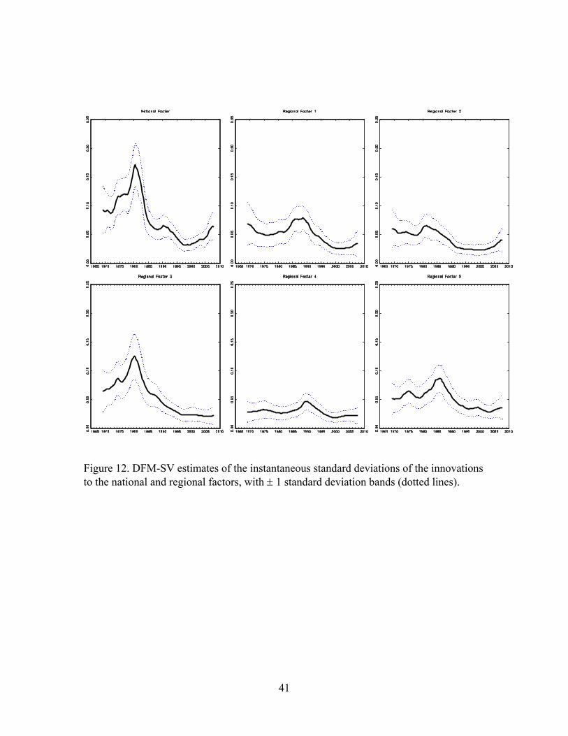
41

Figure 12. DFM-SV estimates of the instantaneous standard deviations of the innovations to the national and regional factors, with ± 1 standard deviation bands (dotted lines).

42

Figure 13. DFM-SV estimates of the evolution of the state-level factor model: the standard deviation of the idiosyncratic innovation (upper left) and the partial R2 from the national factor (upper right), the regional factor (lower left), and the idiosyncratic term (lower right). Shown are the 10%, 25%, 50%, 75%, and 90% percentiles across states, evaluated quarter by quarter.