The exam is of 2 hours & Marks :40

The exam is of two parts ( Part I & Part II)

Part I is of 20 questions . Answer any 15 questionsEach question is of 2 marks . Total 30 marks.

Part II is of 15 questions. Answer any 10 questionsEach question is of 1 mark. Total 10 marks.

No MCQ’s. You should write the answers.

No major calculations. No need to memorize the formulas.

Bring your own calculator. Cell phones are not allowed to use as a calculator.

Study DesignsLevels of measurements (Type of data)Sampling Distribution of Means and proportionsNormal DistributionHypothesis testing & Z- testStudent’s t-testChi -square test, MacNemar’s Chi-square testConfidence IntervalsHow to write a research paper ? ----- ( 40 marks)

QUALITATIVE DATA (Categorical data) DISCRETE QUANTITATIVE CONTINOUS QUANTITATIVE

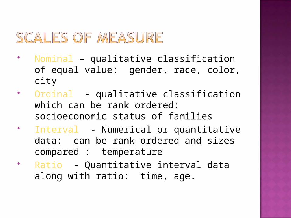
Nominal – qualitative classification of equal value: gender, race, color, city

Ordinal - qualitative classification which can be rank ordered: socioeconomic status of families

Interval - Numerical or quantitative data: can be rank ordered and sizes compared : temperature

Ratio - Quantitative interval data along with ratio: time, age.

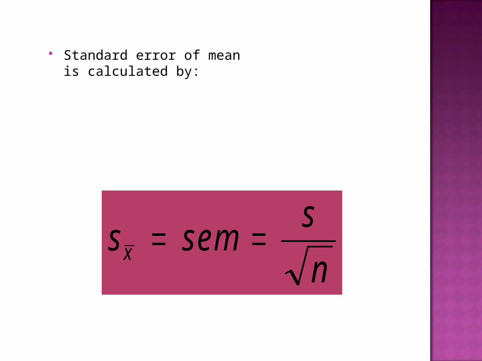
Standard error of mean is calculated by:

s sems

nx

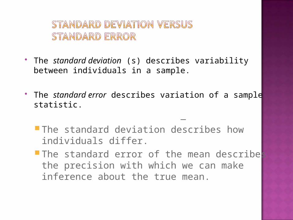
The standard deviation (s) describes variability between individuals in a sample.

The standard error describes variation of a sample statistic.

The standard deviation describes how individuals differ.

The standard error of the mean describes the precision with which we can make inference about the true mean.

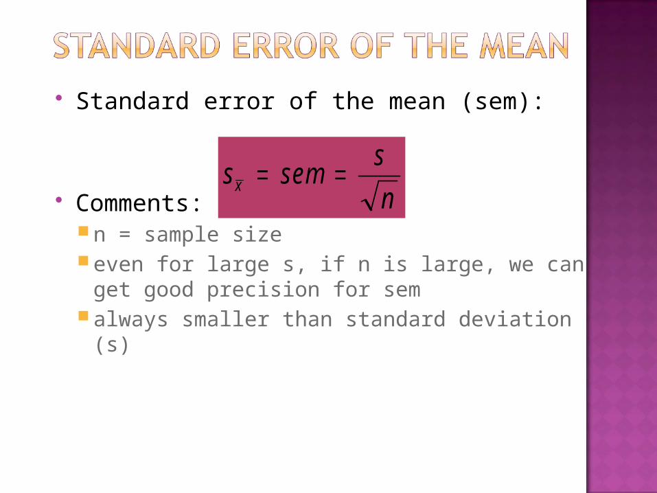
Standard error of the mean (sem):

Comments:n = sample sizeeven for large s, if n is large, we can get good

precision for semalways smaller than standard deviation (s)

s sems

nx

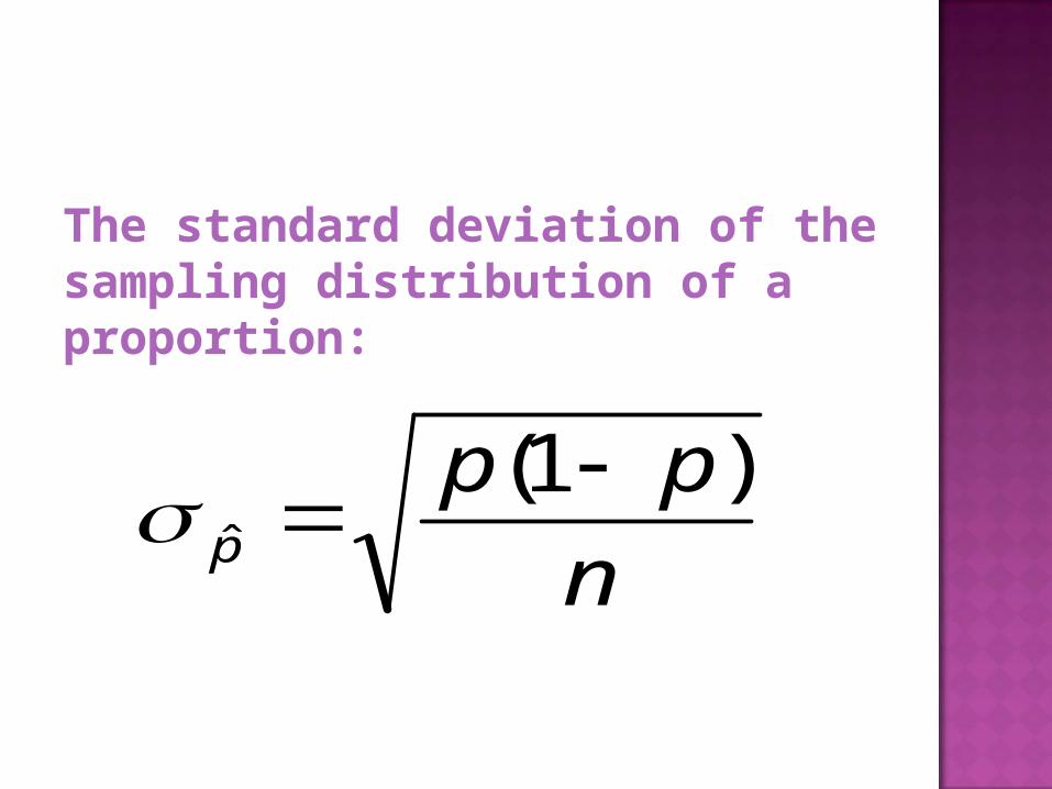
The standard deviation of the sampling distribution of a proportion:

n

ppp

)1(ˆ

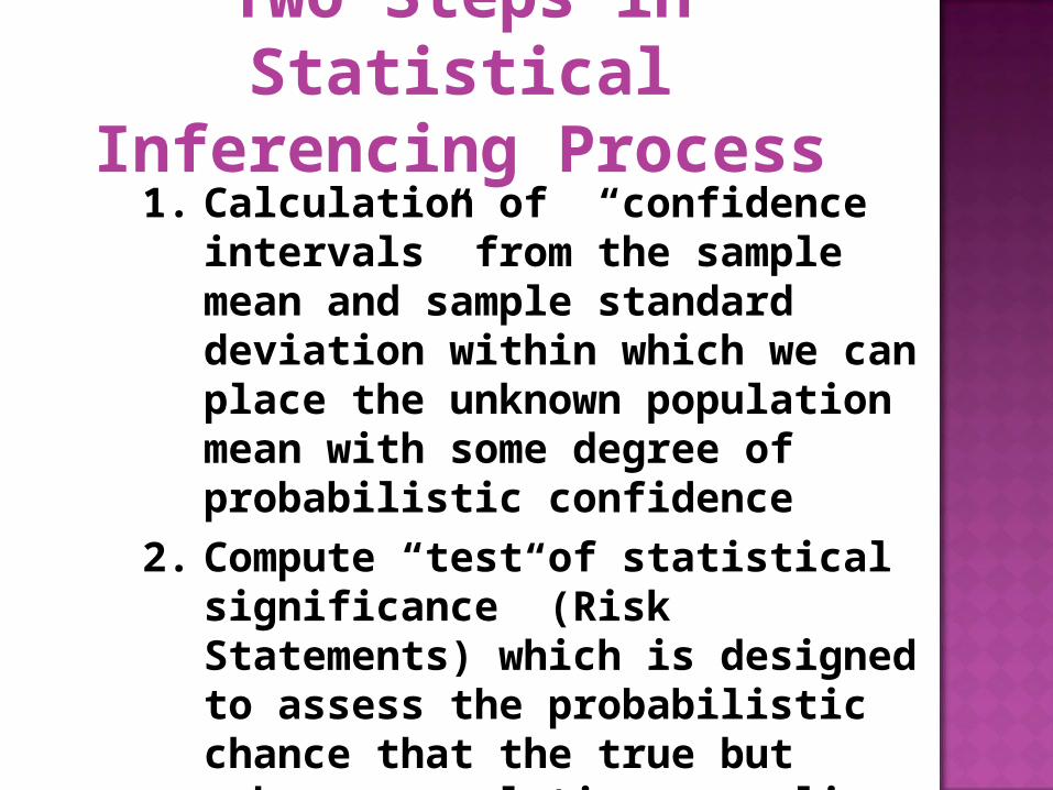
Two Steps in Statistical Inferencing Process

1. Calculation of “confidence intervals” from the sample mean and sample standard deviation within which we can place the unknown population mean with some degree of probabilistic confidence

2. Compute “test of statistical significance” (Risk Statements) which is designed to assess the probabilistic chance that the true but unknown population mean lies within the confidence interval that you just computed from the sample mean.

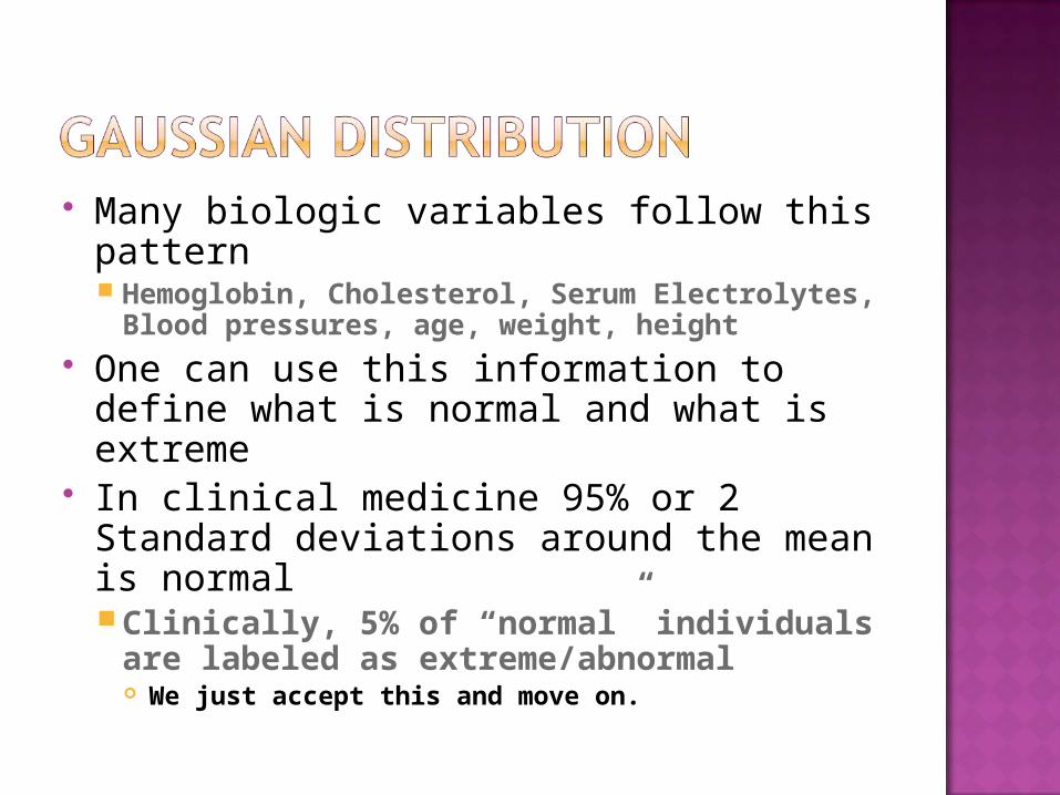
Many biologic variables follow this pattern Hemoglobin, Cholesterol, Serum

Electrolytes, Blood pressures, age, weight, height

One can use this information to define what is normal and what is extreme

In clinical medicine 95% or 2 Standard deviations around the mean is normalClinically, 5% of “normal” individuals

are labeled as extreme/abnormal We just accept this and move on.

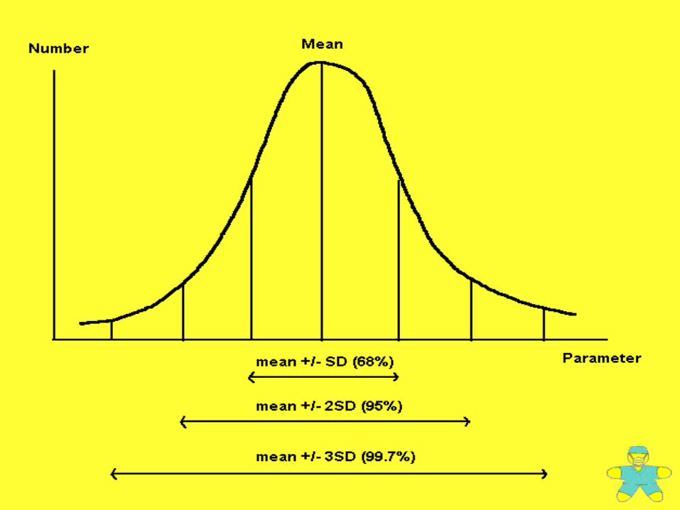
Symmetrical about mean, Mean, median, and mode are equal Total area under the curve above the

x-axis is one square unit 1 standard deviation on both sides of

the mean includes approximately 68% of the total area2 standard deviations includes

approximately 95% 3 standard deviations includes

approximately 99%

Normal distribution is completely determined by the parameters and Different values of shift the distribution

along the x-axis Different values of determine degree of

flatness or peakedness of the graph

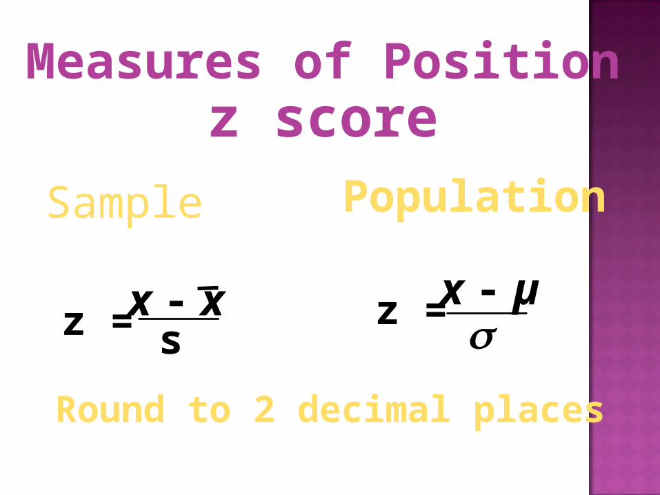
Sample

z =x - xs

Population

z = x - µ

Round to 2 decimal places

Measures of Positionz score

The Z score makes it possible, under some circumstances, to compare scores that originally had different units of measurement.

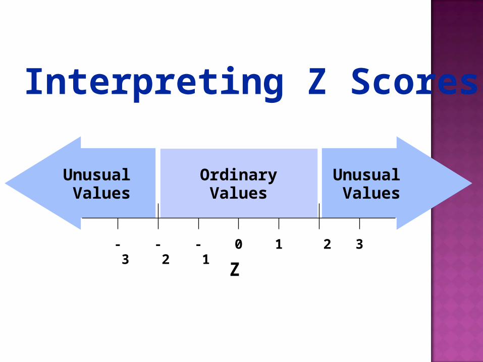
- 3 - 2 - 1 0 1 2 3

Z

Unusual Values

Unusual Values

OrdinaryValues

Interpreting Z Scores

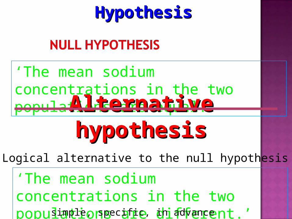
‘The mean sodium concentrations in the two populations are equal.’

Alternative hypothesisAlternative hypothesisLogical alternative to the null hypothesis

‘The mean sodium concentrations in the two populations are different.’

HypothesisHypothesis

simple, specific, in advance

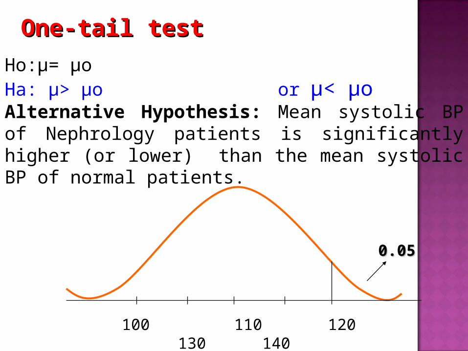
100 110 120 130 140

One-tail testOne-tail test

Ho:μ= μoHa: μ> μo or μ< μo

Alternative Hypothesis: Mean systolic BP of Nephrology patients is significantly higher (or lower) than the mean systolic BP of normal patients.

0.050.05

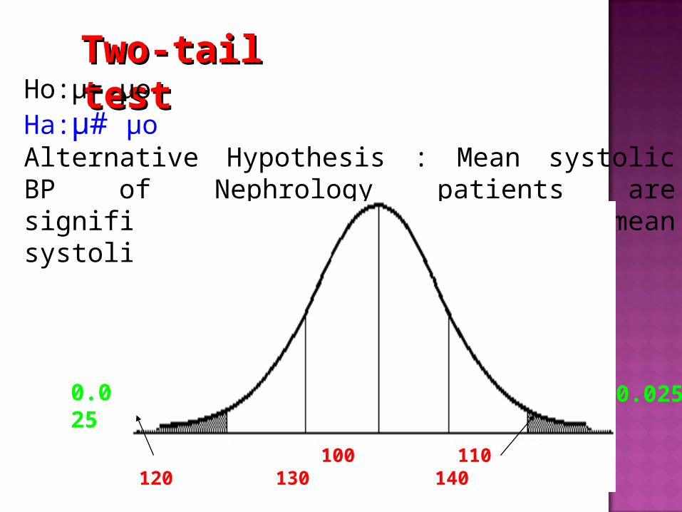
Two-tail testTwo-tail testHo:μ= μo

Ha:μ# μo

Alternative Hypothesis : Mean systolic BP of Nephrology patients are significantly different from mean systolic BP of normal patients.

100 110 120 130 140

0.0250.025

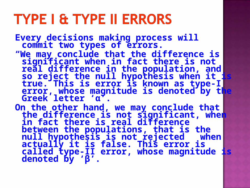
Every decisions making process will commit two types of errors.

“We may conclude that the difference is significant when in fact there is not real difference in the population, and so reject the null hypothesis when it is true. This is error is known as type-I error, whose magnitude is denoted by the Greek letter ‘α’.

On the other hand, we may conclude that the difference is not significant, when in fact there is real difference between the populations, that is the null hypothesis is not rejected when actually it is false. This error is called type-II error, whose magnitude is denoted by ‘β’.

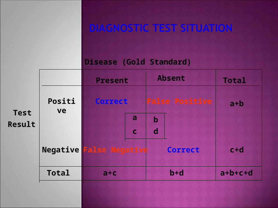
Disease (Gold Standard)

Present

Correct

Negative

Total

PositiveTest

False Negative

a+b

a+b+c+d

Total

Correct

a+c

b+d

c+d

False Positive

Result

Absent

a b

c d

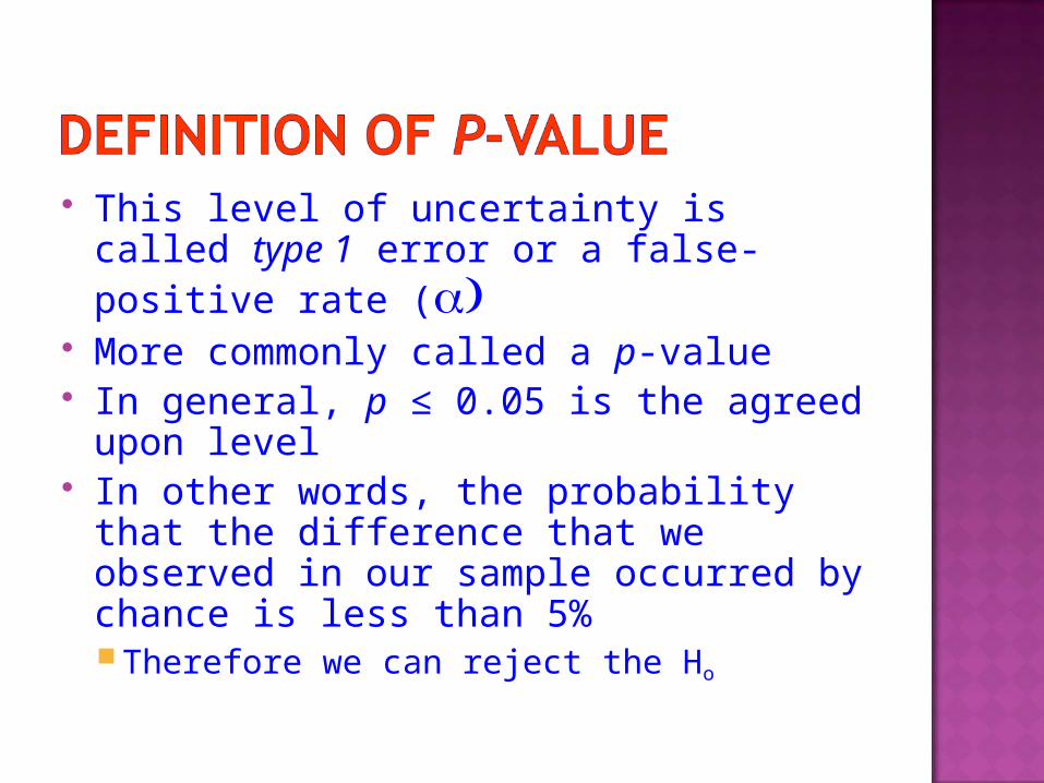
This level of uncertainty is called type 1 error or a false-positive rate (

More commonly called a p-value In general, p ≤ 0.05 is the agreed upon

level In other words, the probability that the

difference that we observed in our sample occurred by chance is less than 5%Therefore we can reject the Ho

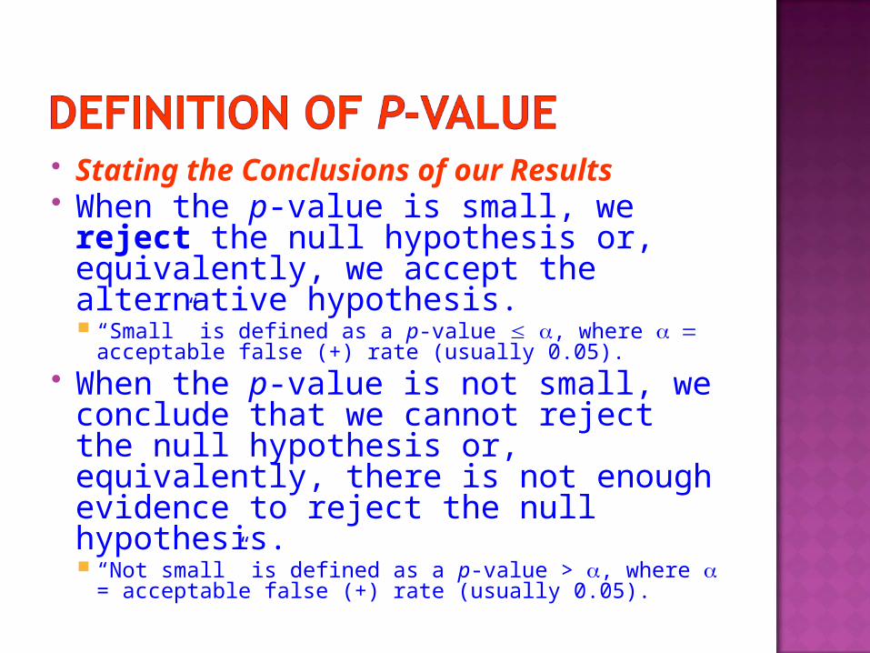
Stating the Conclusions of our Results

When the p-value is small, we reject the null hypothesis or, equivalently, we accept the alternative hypothesis. “Small” is defined as a p-value , where

acceptable false (+) rate (usually 0.05). When the p-value is not small, we

conclude that we cannot reject the null hypothesis or, equivalently, there is not enough evidence to reject the null hypothesis. “Not small” is defined as a p-value > , where =

acceptable false (+) rate (usually 0.05).

P-valueP-value A standard device for reporting quantitative results in research where variability plays a large role.

Measures the dissimilarity between two or more sets of measures or between one set of measurements and a standard.

“ the probability of obtaining the study results by chance if the null hypothesis is true”

“The probability of obtaining the observed value (study results) as extreme as possible”

P-value - continued P-value - continued

“ The p-value is actually a probability, normally the probability of getting a result as extreme as or more extreme than the one observed if the dissimilarity is entirely due to variability of measurements or patients response, or to sum up, due to chance alone”.

Small p value - the rare event has occurredLarge p value - likely event

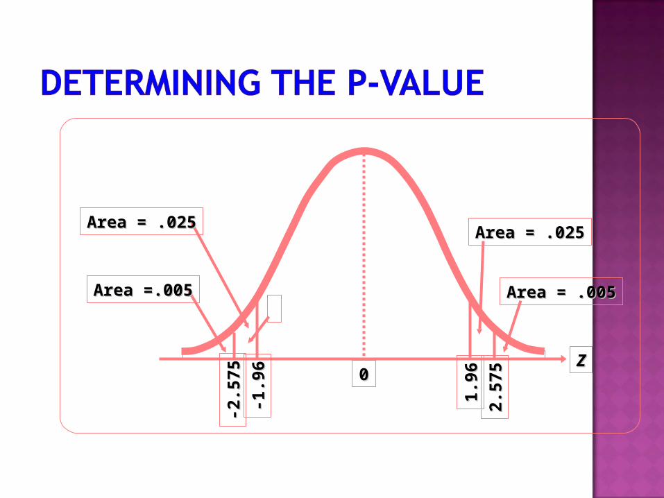
-1.9

6-1

.96 00

Area = .025Area = .025

Area =.005Area =.005

ZZ

-2.5

75

-2.5

75

Area = .025Area = .025

Area = .005Area = .005

1.9

61.9

6

2.5

75

2.5

75

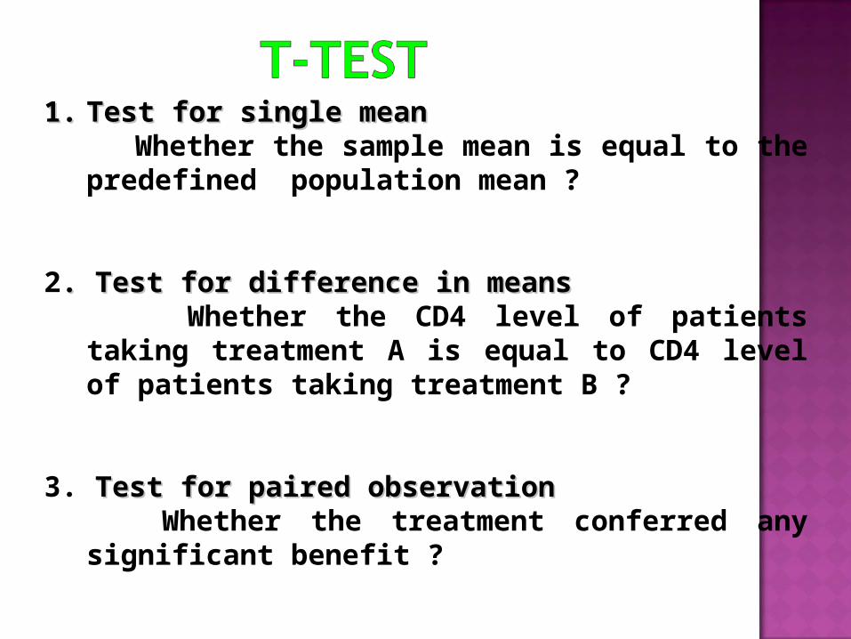
1.1. Test for single meanTest for single mean Whether the sample mean is equal to the predefined

population mean ?

2. Test for difference in means. Test for difference in means Whether the CD4 level of patients taking treatment A is

equal to CD4 level of patients taking treatment B ?

3. Test for paired observationTest for paired observation Whether the treatment conferred any significant benefit ?

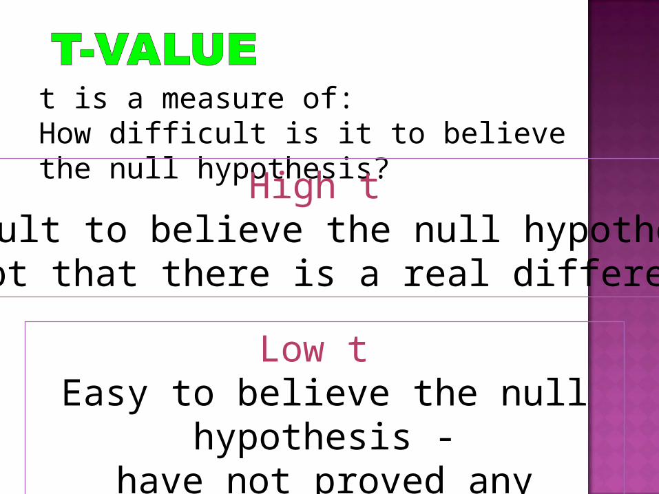
t is a measure of:How difficult is it to believe the null hypothesis?

High t Difficult to believe the null hypothesis -

accept that there is a real difference.

Low t Easy to believe the null hypothesis -

have not proved any difference.

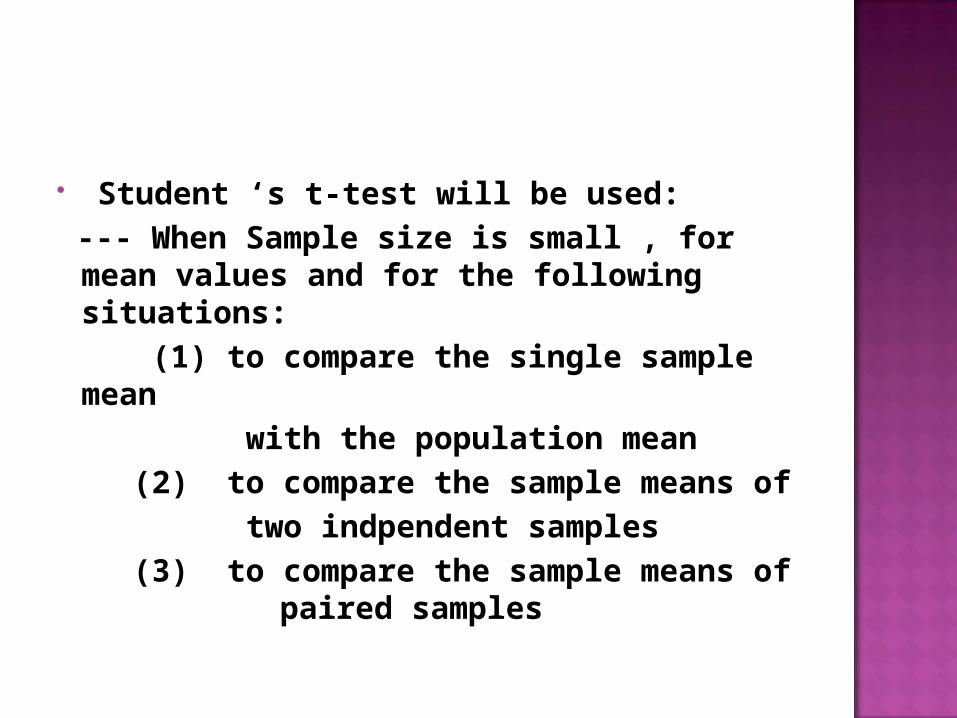
Student ‘s t-test will be used: --- When Sample size is small , for

mean values and for the following situations:

(1) to compare the single sample mean

with the population mean (2) to compare the sample means of two indpendent samples (3) to compare the sample means of

paired samples

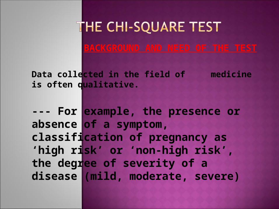
BACKGROUND AND NEED OF THE TEST

Data collected in the field of medicine is often qualitative.

--- For example, the presence or absence of a symptom, classification of pregnancy as ‘high risk’ or ‘non-high risk’, the degree of severity of a disease (mild, moderate, severe)

The measure computed in each instance is a proportion, corresponding to the mean in the case of quantitative data such as height, weight, BMI, serum cholesterol.

Comparison between two or more proportions, and the test of significance employed for such purposes is called the “Chi-square test”

McNemar’s testMcNemar’s test

Situation:Situation:

Two paired binary variables that Two paired binary variables that form a particular type of 2 x 2 form a particular type of 2 x 2 tabletable

e.g. matched case-control study or e.g. matched case-control study or cross-over trialcross-over trial

When both the study variables and outcome variables are categorical (Qualitative):

Apply (i) Chi square test(ii) Fisher’s exact test (Small samples)(iii) Mac nemar’s test ( for paired

samples)

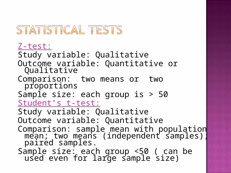
Z-test:Study variable: QualitativeOutcome variable: Quantitative or QualitativeComparison: two means or two proportionsSample size: each group is > 50Student’s t-test:Study variable: QualitativeOutcome variable: QuantitativeComparison: sample mean with population

mean; two means (independent samples); paired samples.

Sample size: each group <50 ( can be used even for large sample size)

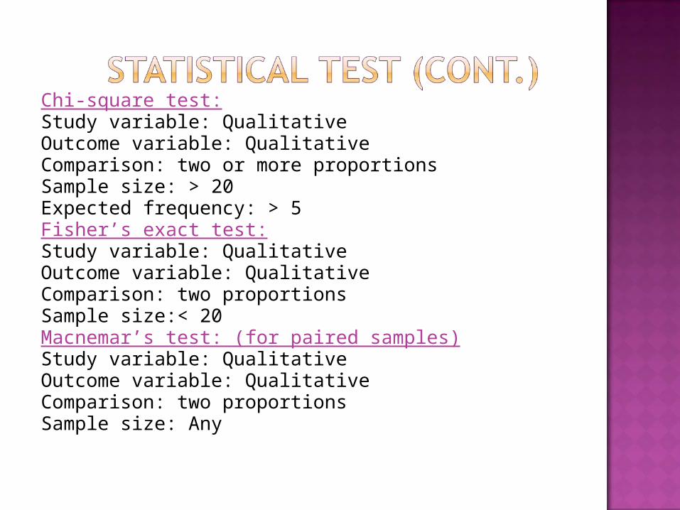
Chi-square test:Study variable: QualitativeOutcome variable: QualitativeComparison: two or more proportionsSample size: > 20Expected frequency: > 5Fisher’s exact test:Study variable: QualitativeOutcome variable: QualitativeComparison: two proportionsSample size:< 20Macnemar’s test: (for paired samples)Study variable: QualitativeOutcome variable: QualitativeComparison: two proportionsSample size: Any

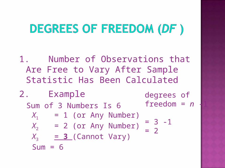
1. Number of Observations that Are Free to Vary After Sample Statistic Has Been Calculated

2. ExampleSum of 3 Numbers Is 6

X1 = 1 (or Any Number)X2 = 2 (or Any Number)X3 = 3 (Cannot Vary)Sum = 6

degrees of freedom = n -1 = 3 -1= 2

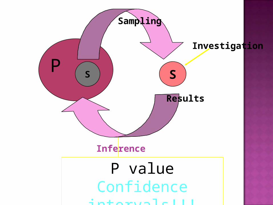
P S

Investigation

S

Sampling

P valueConfidence intervals!!!

Inference

Results

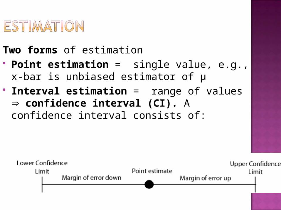
Two forms of estimation Point estimation = single value, e.g., x-bar

is unbiased estimator of μ Interval estimation = range of values

confidence interval (CI). A confidence interval consists of:

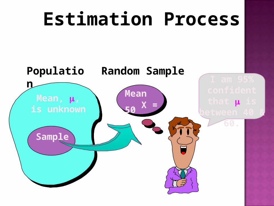
Mean, , is unknown

Population

Random Sample I am 95%

confident that is between 40 &

60.

Mean X = 50

Estimation Process

Sample

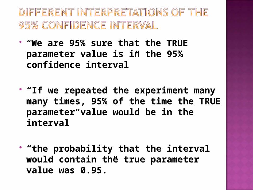
“We are 95% sure that the TRUE parameter value is in the 95% confidence interval”

“If we repeated the experiment many many times, 95% of the time the TRUE parameter value would be in the interval”

“the probability that the interval would contain the true parameter value was 0.95.”

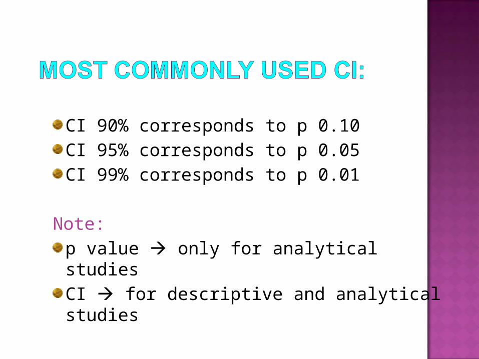
CI 90% corresponds to p 0.10CI 95% corresponds to p 0.05CI 99% corresponds to p 0.01

Note:p value only for analytical studiesCI for descriptive and analytical studies

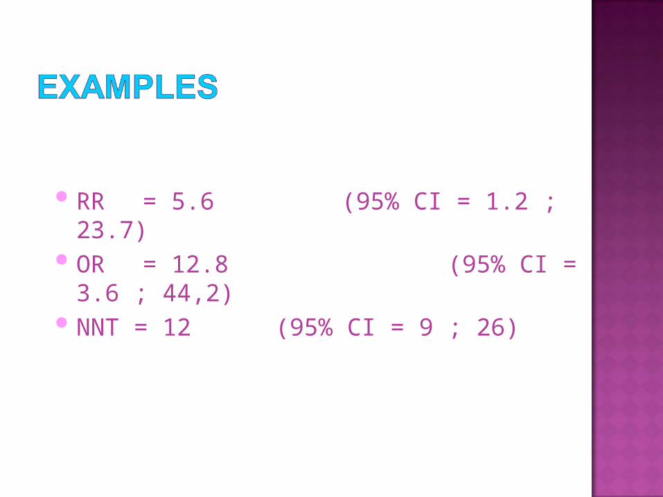
RR = 5.6 (95% CI = 1.2 ; 23.7) OR = 12.8 (95% CI = 3.6 ; 44,2) NNT = 12 (95% CI = 9 ; 26)

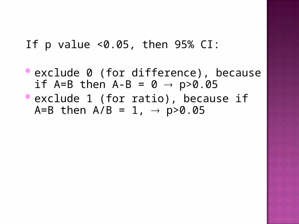
If p value <0.05, then 95% CI:

exclude 0 (for difference), because if A=B then A-B = 0 p>0.05

exclude 1 (for ratio), because if A=B then A/B = 1, p>0.05

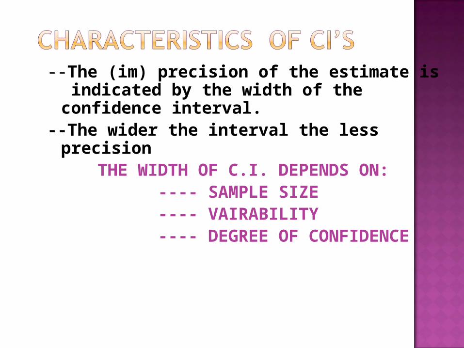
--The (im) precision of the estimate is indicated by the width of the confidence interval.

--The wider the interval the less precision THE WIDTH OF C.I. DEPENDS ON: ---- SAMPLE SIZE ---- VAIRABILITY ---- DEGREE OF CONFIDENCE

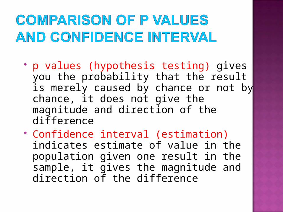
p values (hypothesis testing) gives you the probability that the result is merely caused by chance or not by chance, it does not give the magnitude and direction of the difference

Confidence interval (estimation) indicates estimate of value in the population given one result in the sample, it gives the magnitude and direction of the difference

Abstract Introduction Methods Results Discussion and References

Wishing all of you Best of Luck !