Embed Size (px)
Citation preview

The expansion of modern agriculture and global biodiversity decline: an integrated assessment Bruno Lanz, Simon Dietz and Tim Swanson
May 2017
Grantham Research Institute on Climate Change and the Environment Working Paper No. 167

The Grantham Research Institute on Climate Change and the Environment was established by the London School of
Economics and Political Science in 2008 to bring together international expertise on economics, finance, geography, the
environment, international development and political economy to create a world-leading centre for policy-relevant
research and training. The Institute is funded by the Grantham Foundation for the Protection of the Environment and the
Global Green Growth Institute. It has nine research programmes:
1. Adaptation and development
2. Carbon trading and finance
3. Ecosystems, resources and the natural environment
4. Energy, technology and trade
5. Future generations and social justice
6. Growth and the economy
7. International environmental negotiations
8. Modelling and decision making
9. Private sector adaptation, risk and insurance
More information about the Grantham Research Institute on Climate Change and the Environment can be found at:
www.lse.ac.uk/grantham.

The expansion of modern agriculture and global biodiversity
decline: An integrated assessment∗
Bruno Lanz † Simon Dietz ‡ Tim Swanson §
This version: March 2017
Abstract
The world is banking on a major increase in food production, if the dietary needs and food
preferences of an increasing, and increasingly rich, population are to be met. This requires
the further expansion of modern agriculture, but modern agriculture rests on a small number
of highly productive crops and its expansion has led to a significant loss of global biodiver-
sity. Ecologists have shown that biodiversity loss results in lower plant productivity, while
agricultural economists have linked biodiversity loss on farms with increasing variability of
crop yields, and sometimes lower mean yields. In this paper we consider the macro-economic
consequences of the continued expansion of particular forms of intensive, modern agriculture,
with a focus on how the loss of biodiversity affects food production. We employ a quantita-
tive, structurally estimated model of the global economy, which jointly determines economic
growth, population and food demand, agricultural innovations and land conversion. We show
that even small effects of agricultural expansion on productivity via biodiversity loss might be
sufficient to warrant a moratorium on further land conversion.
Keywords: Agricultural productivity; biodiversity; endogenous growth; food security; land
conversion; population
JEL Classifications: N10; N50; O31; O44; Q15; Q16; Q57.
∗We thank Alex Bowen, Derek Eaton, Sam Fankhauser, Timo Goeschl, David Laborde, Robert Mendelsohn, Anouch Missirian, David Simpson, Marty Weitzman, and seminar participants at LSE, the University of Cape Town, IUCN, SURED 2014, Bioecon 2013, and the Foodsecure Workshop. Excellent research assistance was provided by Arun Jacob. Funding from the MAVA Foundation is gratefully acknowledged. All errors are ours.†Corresponding author. University of Neuchâtel, Department of Economics and Business, Switzerland; ETH Zurich,
Chair for Integrative Risk Management and Economics, Switzerland; Massachusetts Institute of Technology, Joint Pro-gram on the Science and Policy of Global Change, USA. Mail: A.-L. Breguet 2, CH-2000 Neuchâtel, Switzerland; Tel:+41 32 718 14 55; email: [email protected].‡London School of Economics and Political Science, Grantham Research Institute on Climate Change and the Envi-
ronment, and Department of Geography and Environment, UK.§Graduate Institute of International and Development Studies, Department of Economics and Centre for Internatio-
nal Environmental Studies, Switzerland.
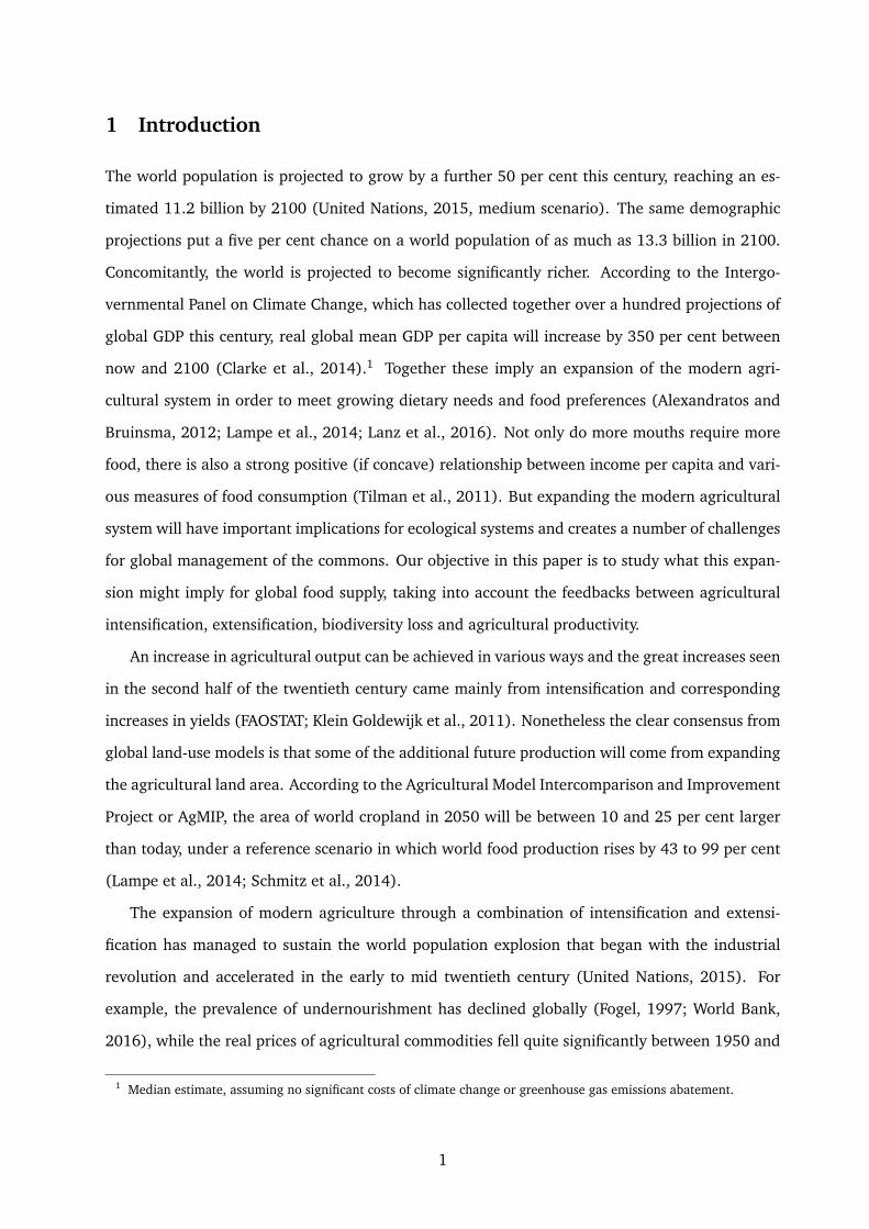
1 Introduction
The world population is projected to grow by a further 50 per cent this century, reaching an es-
timated 11.2 billion by 2100 (United Nations, 2015, medium scenario). The same demographic
projections put a five per cent chance on a world population of as much as 13.3 billion in 2100.
Concomitantly, the world is projected to become significantly richer. According to the Intergo-
vernmental Panel on Climate Change, which has collected together over a hundred projections of
global GDP this century, real global mean GDP per capita will increase by 350 per cent between
now and 2100 (Clarke et al., 2014).1 Together these imply an expansion of the modern agri-
cultural system in order to meet growing dietary needs and food preferences (Alexandratos and
Bruinsma, 2012; Lampe et al., 2014; Lanz et al., 2016). Not only do more mouths require more
food, there is also a strong positive (if concave) relationship between income per capita and vari-
ous measures of food consumption (Tilman et al., 2011). But expanding the modern agricultural
system will have important implications for ecological systems and creates a number of challenges
for global management of the commons. Our objective in this paper is to study what this expan-
sion might imply for global food supply, taking into account the feedbacks between agricultural
intensification, extensification, biodiversity loss and agricultural productivity.
An increase in agricultural output can be achieved in various ways and the great increases seen
in the second half of the twentieth century came mainly from intensification and corresponding
increases in yields (FAOSTAT; Klein Goldewijk et al., 2011). Nonetheless the clear consensus from
global land-use models is that some of the additional future production will come from expanding
the agricultural land area. According to the Agricultural Model Intercomparison and Improvement
Project or AgMIP, the area of world cropland in 2050 will be between 10 and 25 per cent larger
than today, under a reference scenario in which world food production rises by 43 to 99 per cent
(Lampe et al., 2014; Schmitz et al., 2014).
The expansion of modern agriculture through a combination of intensification and extensi-
fication has managed to sustain the world population explosion that began with the industrial
revolution and accelerated in the early to mid twentieth century (United Nations, 2015). For
example, the prevalence of undernourishment has declined globally (Fogel, 1997; World Bank,
2016), while the real prices of agricultural commodities fell quite significantly between 1950 and
1 Median estimate, assuming no significant costs of climate change or greenhouse gas emissions abatement.
1

2000 (Alston and Pardey, 2014).2 However, the expansion of modern agriculture has had other,
less desirable consequences.
Both agricultural intensification – of the prevailing, non-ecological or unsustainable variety
(cf. Bommarco et al., 2013; Godfray and Garnett, 2014) – and extensification have been primary
causes of an historically unprecedented loss of global biodiversity. According to the Millennium
Ecosystem Assessment (2005), the current global rate of species extinction is up to 1000 times
higher than the background rate that has been estimated from the fossil record. A broader index
of global biodiversity has been in decline since 1970 (the first year for which data are available)
and there is no statistical indication that the rate of decline is slowing (Butchart et al., 2010).
Local species richness is estimated to have declined by over 10% in the last 200 years, globally on
average (Newbold et al., 2015).
In terms of agricultural biodiversity, Khoury et al. (2014) have documented how global crop
production has become less diverse in the last 50 years, in the sense that it has become more
dominated by a small number of crops. Using data from the Food and Agriculture Organization
of the United Nations (FAO), they show that, while national food supplies have come to rely on a
more diverse set of crops on average, the opposite is true of the global food supply. Although this
might seem paradoxical at first, it is in fact because the same crops have been driving both greater
diversity in most countries (particularly developing countries) and greater similarity globally:
wheat, rice, soybeans and oil crops such as palm oil and sunflowers. These are precisely the crops
we would expect to become more prevalent as diets change with rising incomes (Poleman and
Thomas, 1995). In addition to inter-specific diversity of crops, nearly all countries reporting to
the FAO’s global stocktake of crop genetic diversity documented the erosion of genetic diversity,
with the most commonly identified causes being respectively the replacement of local varieties as
part of the modernization of production systems, and land clearing (FAO, 1996, 2010).
Following a proliferation of research in the last 25 years, there is now a consensus that bi-
odiversity at different levels increases the plant productivity of natural ecosystems, as well as
reducing the variability of plant productivity (Cardinale et al., 2012). Plant productivity decrea-
ses more than proportionally as biodiversity is lost. Once more than 20% of species are lost, the
effects may rival other drivers of global environmental change such as planetary warming, ozone
and acidification (Cardinale et al., 2012; Hooper et al., 2012). While the negative relationship
2 Since 2000 they have been on a slightly increasing trend.
2

between biodiversity loss and plant productivity is reliably found in natural ecosystems such as
grasslands, it is clearly possible for intensively managed monocultures to be highly productive.
Nonetheless a recurrent finding from empirical studies by agricultural economists is that genetic
and species diversity on farms reduces the variability of crop yields and sometimes increases the
mean yield (see Di Falco, 2012, for a review of these studies). This has been found not only in
low-intensity, biologically diverse farming systems such as Ethiopia (Di Falco et al., 2010) and
Pakistan (Smale et al., 1998), but also in high-intensity, low-biodiversity farming systems such as
the East of England (Omer et al., 2007).
There are several reasons why more biologically diverse farming systems would display lower
yield variability, and sometimes higher mean yields. These include symbiotic interactions and
resource-use complementarities between species, as well as statistical averaging between species
that respond differently to exogenous shocks such as extreme weather, pests and pathogens (Til-
man, 1999). This is a portfolio effect (Baumgärtner, 2007) that is also provided within crop
species by genetic diversity. In the ecological literature, there is a particular emphasis on how
biologically diverse farming systems can be less vulnerable to pests and pathogens thanks to these
kinds of mechanism. Pests and pathogens have a very significant impact on global crop yields,
with direct losses estimated to be in the range of 20 to 40 per cent (Oerke, 2006; Savary et al.,
2012). A famous example is the potato famine of 1845-8 that contributed to 1.5 million deaths in
Ireland. Furthermore, expanding the agricultural land area reduces the extent of natural reserve
lands, so that the pool of genetic material that can potentially be used as an input to agricultural
R&D activities decreases (Simpson et al., 1996; Rausser and Small, 2000).
In this work we explore the implications of global biodiversity loss, caused by the expansion
of modern agriculture, for agricultural production itself. At the extensive margin, the conversion
of natural lands into modern agriculture is undertaken with the intention of increasing the pro-
duction of food, but at the same time the evidence we have just presented suggests it imposes
a risk on agricultural productivity, through the loss of biodiversity on natural and agricultural
land.3 The creation of this risk to global agricultural productivity results from individual decisi-
ons. Profit-maximizing farmers clear land and plant it with small numbers of high-yielding crop
varieties, leading to the loss of biodiversity at the local and global scales. In this process, farmers
3 From the evidence presented by Khoury et al. (2014), for instance, we might assume that agriculture at the exten-sive margin displays lower-than-average crop and genetic diversity.
3

only partially take into account their marginal impact on biodiversity, and in turn on agricultural
productivity (Bowman and Zilberman, 2013; Heal et al., 2004; Weitzman, 2000). Decisions at the
individual level about land conversion and crop selection thus cause an externality with respect
to aggregate production.
To study the socially optimal expansion of agricultural land in this setting, we employ a quanti-
tative two-sector endogenous growth model of the global economy. We represent the biodiversity
externality by means of a global-level hazard function, which links cropland conversion with de-
preciation of agricultural productivity. This is in the spirit of damage functions in integrated
assessment models of climate change (e.g. Nordhaus, 1992; Nordhaus and Boyer, 2000), which,
despite legitimate concerns about their predictive capabilities, have proved fundamental to our
understanding of that problem. Our growth model has a number of other features, which enable
us to derive insights about the interactions between global economic growth and the impact of
declining biodiversity on food production. In order to characterize agriculture’s role in producing
food and sustaining population, the model distinguishes agriculture from other economic activi-
ties. Demand for food in the model is proportional to the size of the population and it increases
with per-capita income. The world population is endogenously determined by households’ prefe-
rences for fertility (Barro and Becker, 1989), as well as the opportunity cost of raising children,
which is itself linked with technical progress in the economy (Galor and Weil, 2000). Technical
progress in agriculture and the rest of the economy is therefore key and it is modeled as Schum-
peterian innovation (Aghion and Howitt, 1992), whereby total factor productivity (TFP) growth
requires labor as an input to R&D activities. The model is structurally estimated to fit 1960-2010
data on world GDP, population, TFP growth and cropland area, providing an empirical framework
to study the socially optimal allocation of land to meet the growing demand for food in the future.
In the absence of the biodiversity externality, we project that world population increases by
about 40 per cent by 2050, world GDP doubles and cropland area increases by about 7 per cent.
In 2100 the world population reaches about 12.4 billion. In the presence of the externality, the
global-level hazard function links cropland conversion with depreciation of agricultural TFP. This
means agricultural innovation is a contest between man-made R&D on the one hand and natural
depreciation from biodiversity loss on the other hand (Goeschl and Swanson, 2003). We first
consider the socially optimal response from a global perspective. Our model suggests that a social
planner would respond by immediately preventing the further expansion of cropland, as well as
4

allocating more labor to agricultural production and agricultural R&D, with negligible effects on
fertility and population. Given that the planner can select the least-cost management strategy to
tackle the biodiversity externality, and that land is assumed to be relatively easily substituted in
agricultural production (the elasticity of substitution between land and other factors is 0.6, which
is taken from Wilde, 2013), we find that the welfare cost is small.
We then consider situations in which managing the externality might impose greater social
costs. First, we solve the model under the assumption that fertility and land-conversion choi-
ces cannot feasibly be controlled by a global social planner. Instead, these choices are made in
a decentralized manner by atomistic farming households, who do not take into account the bi-
odiversity externality. In this scenario, the planner increases the share of labor in agricultural
production and agricultural R&D, in order to counter TFP depreciation, but the biodiversity ex-
ternality still generates a substantial welfare cost, suggesting a global policy to limit cropland
expansion might have significant value. Second, we consider lower substitutability of land in
agricultural production (the elasticity of substitution between land and other factors is lowered
to 0.2) and how this affects the optimal response of the global social planner. In this scenario,
the reduction of cropland is significantly lower, and, despite allocating more labor to agricultural
production and agricultural R&D, the welfare cost is again larger.
The remainder of the paper is structured as follows. Section 2 describes the model and its
estimation on historical data, while Section 3 focuses on the specification and parametrization
of the biodiversity hazard function. The following three sections report our results. Section
4 analyzes the socially optimal use of cropland in the presence of the biodiversity externality,
compared with a baseline scenario without the externality. Section 5 then considers the scenario in
which land-conversion and fertility decisions are decentralized to households. Section 6 analyzes
the effect of lower substitutability of land. Section 7 concludes.
2 The model
This section summarizes the key components of the model and estimation procedure. A com-
prehensive discussion of the structure of the model, selection and estimation of the parameters,
the ensuing projections from the model, as well as sensitivity analysis, is reported in Lanz et al.
5

Figure 1: Schematic representation of the model
Manufacturing
output
YMN Manufacturing
technology
AMN
Labor allocation
NMN, NAG, NA,MN,
NA,AG, NX, NN
Population
N
Agricultural
technology
AMN
Agricultural
land area
X
Savings decision
C / I
Capital stock
K
Capital allocation
KMN, KAG
Welfare
Agricultural
output
YAG
HUMAN CAPITAL
CONSTRAINT
FOOD REQUIREMENTS CONSTRAINT
LEGEND:
Stock variables
Control
variables
(2016).4 A schematic representation of that model is provided in Figure 1. This paper deploys
the model described therein, but adds the hazard function that captures the external cost of land
conversion to agricultural productivity.
2.1 The economy
2.1.1 Production and capital accumulation
The model comprises two sectors: a manufacturing sector that produces the traditional con-
sumption good in one-sector models, and an agricultural sector that produces food to sustain
contemporaneous population. In manufacturing, aggregate output is represented by a standard
Cobb-Douglas production function:
Yt,mn = At,mnKϑt,mnN
1−ϑt,mn , (1)
4 The GAMS code of the model is available from Bruno Lanz’s website.
6

where Yt,mn is real manufacturing output at time t, At,mn is an index of productivity in manufac-
turing, Kt,mn is capital allocated to manufacturing, and Nt,mn is the manufacturing workforce. We
assume that technology is Hicks-neutral, so that the Cobb-Douglas functional form is consistent
with long-term empirical evidence (Antràs, 2004). We use a standard value of 0.3 for the share of
capital (see, for example, Gollin, 2002).
Agricultural production requires land services Xt as an input and, following Kawagoe et al.
(1986) and Ashraf et al. (2008), we employ a nested constant-elasticity-of-substitution (CES)
function to represent substitution possibilities between land and a capital-labor composite:5
Yt,ag = At,ag
[(1− θX)
(KθKt,agN
1−θKt,ag
)σ−1σ
+ θXXσ−1σ
t
] σσ−1
, (2)
where σ is the elasticity of substitution between the capital-labor composite and agricultural land.
We set σ = 0.6 based on long-run empirical evidence reported in Wilde (2013).6 We come back
to the importance of this parameter for our results in Section 6 below. We further set θX = 0.25
and θK = 0.3, consistent with data reported in Hertel et al. (2012).
2.1.2 Innovations and technological progress
As in the Schumpeterian model of Aghion and Howitt (1992), sectoral TFP evolves according to
At+1,j = At,j · (1 + ρt,jS) , j ∈ {mn, ag} , (3)
where S is the maximum growth rate of TFP each period and ρt,j ∈ [0, 1] is the arrival rate of
innovations each period. Actual sectoral TFP growth is then the share of the maximum feasible
TFP growth (we set S = 0.05 based on Fuglie, 2012) and depends on the number of innovations
arriving within each time period.7 The rate at which innovations arrive in each sector is a function
5 A Cobb-Douglas function is often used for agriculture, notably in Mundlak (2000) and Hansen and Prescott (2002).However, this implies that, in the limit, land is not an essential input to agriculture, with drawbacks that have beenextensively discussed in relation to the scarcity of non-renewable resources (see Dasgupta and Heal, 1979, for aseminal contribution).
6 The estimate by Wilde (2013) is based on 550 years of data from pre-industrial England, thus reflecting long-termsubstitution possibilities, and is estimated in a way that is consistent with our CES functional form (2). However,external validity may be an issue, in particular when applying results for pre-industrial England to developingcountries with rapidly growing population. In the discussion of the results below, we also consider the case ofσ = 0.2.
7 In the original work of Aghion and Howitt (1992), time is continuous and the arrival of innovations is modeled asa Poisson process. Our representation is qualitatively equivalent, but somewhat simpler, as ρt,j implicitly uses thelaw of large number to smooth out the random nature of innovations over discrete time periods.
7

of labor allocated to sectoral R&D:
ρt,j = λj
(Nt,Aj
Nt
)µj, j ∈ {mn, ag} ,
where Nt,Aj is labor employed in R&D in sector j, λj > 0 is a productivity parameter and µj ∈
(0, 1) is an elasticity. This formulation implies that TFP growth increases with the share of labor
allocated to the R&D sector, rather than the absolute amount (Chu et al., 2013). The latter
implication, known as the ‘scale effect’, is not supported by data (Jones, 1995).8 Furthermore,
our representation of R&D implies decreasing returns to labor in R&D through the parameter µj ,
which captures the duplication of ideas among researchers (Jones and Williams, 2000).
The parameter λj is normalized to unity to ensure that TFP growth is bounded between 0 and
S, and the parameters µmn and µag are estimated as described below.
2.1.3 Labor and population dynamics
In each period, the change in world population is given by the difference between fertility nt and
the rate at which population exits the labor force δN :
Nt+1 = Nt(1− δN ) + ntNt , N0 given . (4)
Since population equals the total labor force in our model, δN is the inverse of the expected
working lifetime, which we set to 45 years (hence the ‘working mortality rate’ is δN = 0.022).
Fertility derives from the allocation of labor to child-rearing activities, so that child-rearing
competes with other labor-market activities:
ntNt = χt ·Nt,N ,
where Nt,N is labor allocated to child-rearing activities and χt is an inverse measure of the time
cost of producing effective labor units. We postulate an increasing relationship between the time
8 Scaling the labor force in R&D by Nt is also in line with micro-foundations of more recent representations oftechnological change. In the models of Dinopoulos and Thompson (1998), Peretto (1998) and Young (1998), R&Dactivities simultaneously develop new products and improve existing ones, and the number of products grows withpopulation, thereby diluting R&D inputs and avoiding the population scale effect. Another strategy to address thescale effect involves postulating a negative relationship between labor productivity in R&D and the existing level oftechnology, giving rise to “semi-endogenous” growth models (Jones, 1995, 2001). In this setup, however, long-rungrowth is only driven by population growth, which is also at odds with the data (Ha and Howitt, 2007).
8

cost of child-rearing and the level of technology:
χt = χN ζ−1t,N /Aωt ,
where χ > 0 is a productivity parameter, ζ ∈ (0, 1) is an elasticity representing scarce factors
required in child-rearing, At is an index of technology and ω > 0 measures how the cost of children
increases with the level of technology. This formulation implies that, as the stock of knowledge in
the economy grows, additions to the stock of effective labor units become increasingly costly. In
other words there is a complementarity between technology and skills (Goldin and Katz, 1998),
which implies that a demographic transition will occur as education requirements increase over
time (Galor and Weil, 2000). The ‘quality’ of children required to keep up with technology will
be favored over the quantity. Furthermore, ζ captures the fact that the cost of child-rearing over
a period of time increases more than proportionally with the number of children (see Barro and
Sala-i Martin, 2004, p.412 and Bretschger, 2013). The parameters determining the cost of fertility
and how it evolves over time (χ, ζ and ω) are estimated from the data, as described below.
Population dynamics are further constrained by food availability, as measured by agricultu-
ral output.9 Specifically, in each period agricultural production is consumed entirely to sustain
contemporaneous population:
Y agt = Ntf t,
where f t is per-capita food demand, i.e. the quantity of food required to maintain an individual in
a given society. We further specify per-capita demand for food as a concave function of per-capita
income:
f = ξ ·(Yt,mn
Nt
)κ,
where ξ is a scale parameter and κ > 0 is the income elasticity of food consumption. Food
demand thus captures both physiological requirements (e.g. minimum per-capita caloric intake)
and the way that preferences imbibe a positive relationship between income and the consumption
9 Food consumption does not contribute directly to social welfare. As discussed below, however, the level of popu-lation enters the social welfare criterion (together with the utility of per-capita consumption of the manufacturinggood). Therefore food availability will affect social welfare through the impact of the subsistence requirement onpopulation. For a similar treatment, see Strulik and Weisdorf (2008), Vollrath (2011) and Sharp et al. (2012).
9

of calories. We set the income elasticity of food demand κ = 0.25, which is consistent with
evidence across countries and over time reported in Subramanian and Deaton (1996), Beatty and
LaFrance (2005), and Logan (2009). The parameter measuring food consumption for unitary
income (ξ) is calibrated such that the demand for food in 1960 represents about 15% of world
GDP, which corresponds to the GDP share of agriculture reported in Echevarria (1997). This
implies ξ = 0.4.
2.1.4 Land
As a primary factor, the land input to agriculture has to be converted from a total stock of available
land X by applying labor. Over time the stock of land used in agriculture develops according to
Xt+1 = Xt(1− δX) + ψ ·N εt,X , X0 given , Xt ≤ X , (5)
where Nt,X is labor allocated to land-clearing activities, ψ > 0 measures labor productivity in
land-clearing activities, ε ∈ (0, 1) is an elasticity, and the depreciation rate δX measures how fast
converted land reverts back to natural land. We assume the period of regeneration of natural land
is 50 years, so that δX = 0.02. The parameters ψ and ε are estimated from the data as described
below.
2.1.5 Preferences and savings
The utility function of a representative household is defined over own consumption of the ma-
nufactured good ct, fertility nt and the utility its children will experience in the future Ui,t+1.
More specifically, we represent household preferences with the recursive formulation of Barro and
Becker (1989):
Ut =c1−γt − 1
1− γ+ βn1−ηt Ui,t+1 ,
where γ is the elasticity of marginal utility of consumption of the manufactured good or in other
words the inverse of the intertemporal elasticity of substitution, β is the discount factor and η
is an elasticity determining how the utility of parents changes with nt. The objective function is
given by the utility function of the dynastic head and obtained by successive substitution of the
10

recursive utility function (see Lanz et al., 2016, for the detailed derivation):
U0 =∞∑t=0
βtN1−ηt
(Ct/Nt)1−γ − 1
1− γ, (6)
where Ct = ctNt is aggregate consumption at t.
The parametrization of the objective function is as follows. First, the elasticity of intertemporal
substitution is set to 0.5 in line with estimates by Guvenen (2006). In the model, this corresponds
to γ = 2. Second, we set η = 0.001 so that altruism towards the welfare of children remains almost
constant as the number of children increases, while at the same time ensuring concavity of the
objective function. This implies the objective function is very close to being Classical Utilitarian.
Third, we set the discount factor to 0.99, which corresponds to a pure rate of time preference of 1
per cent per year.
Aggregate consumption derives from manufacturing output, which can alternatively be inves-
ted into a stock of capital:
Yt,mn = Ct + It , (7)
where Ct and It are aggregate consumption and investment respectively. The accumulation of
capital is then given by:
Kt+1 = Kt(1− δK) + It , K0 given , (8)
where δK is the per-period depreciation rate. Because we solve for the social planner solution of
the problem (see below), savings cum investment decisions mirror those of a one-sector economy
(see Ngai and Pissarides, 2007, for a similar treatment of savings in a multi-sector growth model).
2.2 Estimation of the model
We consider the planner’s problem of selecting the allocation of labor and capital as well as the
saving rate to maximize the utility of a representative dynastic household.10 Specifically, a repre-
10 The fact that we solve the model as a social planner problem simplifies the notation and allows us to exploitefficient solvers for constrained non-linear optimization. However, it abstracts from externalities that would arisein a decentralized equilibrium. As discussed below, however, market imperfections prevailing over the estimationperiod will be reflected in the parameters that we estimate from observed trajectories.
11

sentative household chooses paths forNt,j ,Kt,j , and Ct by maximizing (6) subject to technological
constraints (1), (2), (3), (4), (5), (7), (8) and resource allocation constraints for capital and labor:
Kt = Kt,mn +Kt,ag , Nt = Nt,mn +Nt,ag +Nt,Amn +Nt,Aag +Nt,N +Nt,X .
The numerical model is solved as a constrained non-linear optimization problem and thus mimics
the welfare maximization program by directly searching for a local optimum of the objective
function (the discounted sum of utility) subject to the requirement of maintaining feasibility as
defined by the constraints of the problem.11
As mentioned above, parameters determining the cost of fertility (χ, ζ, ω), labor productivity
in R&D (µmn,ag) and labor productivity in land conversion (ψ, ε) are estimated by fitting the model
to 1960-2010 trajectories for world GDP (Maddison, 1995; Bolt and van Zanden, 2013), popula-
tion (United Nations, 1999, 2013), crop land area (Goldewijk, 2001; Alexandratos and Bruinsma,
2012) and sectoral TFP (Martin and Mitra, 2001; Fuglie, 2012). The estimation procedure in-
cludes three main steps, and is discussed in more detail in Appendix A. First, we impose specific
parameter values for a number of quantities that are standard in the literature (see discussion
above). Second, we calibrate values for the state variables to initialize the model in 1960. Third,
we define a minimum distance criterion for GDP (Yt,mn + Yt,ag), population (Nt), crop land (Xt),
and TFP (At,mn, ag) as a way to select the vector of parameters that best fits the observed trajecto-
ries. Using simulation methods to select the vector of parameters that minimizes our criterion, we
find that the model closely fits the targeted data (see goodness-of-fit measures in Appendix A).
3 Specification of the biodiversity externality
As described above, innovation in agriculture is driven by allocating labor to R&D activities, while
land acts as an input to agricultural production. We now introduce the critical second role of
land allocation, which is to modulate biodiversity loss and in turn the depreciation of agricultural
TFP. The rate of depreciation of agricultural TFP is endogenous and depends on the size of the
agricultural system in terms of global cropland area.
11 The numerical problem is formulated in GAMS and solved with KNITRO (Byrd et al., 1999, 2006), a specializedsoftware for constrained non-linear programs.
12

Agricultural R&D proceeds in a similar fashion to R&D in the manufacturing sector,
At+1,ag = At,ag · (1 + ρt,agS − φtS) , (9)
except that in this case φt measures the rate at which man-made R&D depreciates. This depends
on the amount of cultivatable land allocated to crop production:
φt = λD (Xt)µD , (10)
where λD ≥ 0 and µD > 1, which is consistent with the relationship between biodiversity and
plant productivity in natural ecosystems (Hooper et al., 2012). The expected growth rate of
agricultural TFP is then the net result of the flow of innovations out of man-made R&D (or moves
up the TFP ladder) and the arrival of biological hazards associated with the scale of agriculture
(moves down the technological ladder), in the spirit of Goeschl and Swanson (2003).
While the ecological processes underpinning Equation (10) are well documented (see the In-
troduction), there exists as yet no empirical evidence that can directly guide the parametrization
of an agricultural biodiversity hazard function at the global level. Separately identifying man-
made innovation and natural depreciation of agricultural TFP is challenging in empirical data.12
The large body of ecological experiments is strongly suggestive of a negative relationship between
species diversity and plant productivity that holds globally (Cardinale et al., 2012; Hooper et al.,
2012), but many of these experiments have been conducted outside cropping systems. The em-
pirical evidence from agricultural economics (Di Falco, 2012) is directly relevant, but it is simply
more sparse at this point. We therefore select the parameters determining the scale of the exter-
nality, λD and µD in (10), in order to simply illustrate the processes at play and how these impact
the macro-economy.
We run with two specifications, low and high, as shown in Figure 2. In the low hazard function,
λD = 1.6e− 6 and µD = 10. In the high hazard function, λD = 3.5e− 6 and again µD = 10. Both
functions imply that the TFP depreciation rate is almost insignificant for the area of cropland up to
and including 2010. Under the low hazard function, the impact on TFP depreciation of additional
land conversion beyond the 2010 area remains small, but under the high hazard function it rises
12 However, because the model is fitted to the last 50 years of data on agricultural TFP growth, estimates of laborproductivity in agricultural R&D will reflect the occurrence of biological hazards in the past.
13

Figure 2: Land conversion and expected rate of agricultural TFP depreciation
0.0005
0.001
0.0015
0 0.5 1 1.37 (1960)
Converted agricultural land in billion ha (X)
1.77(2100)
1.62(2010)
1.73(2050)
Low hazard: λD = 1e-6High hazard: λD = 3.5e-6
more sharply. Along our baseline scenario (see below), the global area of cropland reaches around
1.8 billion hectares in 2100 and the high hazard function associates this with a TFP depreciation
rate of around 0.1 per cent. This compares with TFP growth from man-made innovation of around
one per cent in 2010, declining over time to 0.5 per cent. Therefore TFP depreciation is relatively
small, even under the high hazard function. In view of the fact that biodiversity loss has an impact
on crop yield variability, it is appropriate to interpret the hazard function as a certainty equiva-
lent, similar to the treatment of climate damages in Nordhaus’ work with the DICE integrated
assessment model (Nordhaus and Boyer, 2000).
4 Results: optimal management of the biodiversity externality
In this section we consider the socially optimal response under the two hazard schedules, as
well as in a baseline scenario where the biodiversity externality is absent. What is shown is
the outcome of a representative household cum social planner controlling all the variables of
the problem in order to maximize welfare. In the presence of the biodiversity externality, this
implies the social planner can internalize the negative impact of land conversion on agricultural
TFP by conserving natural land and reducing fertility, among other things. In the presence of the
externality, it is indeed appropriate to interpret the representative agent as a social planner rather
14

than a household.13 To begin with, we are particularly interested in how the social planner would
optimally manage the externality. That is why we do not impose the externality on an economy
that is constrained in how it can respond. We return to this issue in the next section.
In the following, we first report aggregate impacts for population, land, technology, and agri-
cultural output. We then turn to the implied reallocation of labor across sectors in response to the
externality. Finally, we quantify the welfare cost of the optimal policy in terms of consumption of
the manufactured good and food.
4.1 Aggregate impacts
Figure 3 displays trajectories for world population (panel a) and global cropland (panel b). The
baseline scenario delivers a world population of 9.8 billion in 2050 and 12.4 bn. in 2100. This
is towards the upper end of the 20-80% confidence interval of the latest UN projections (United
Nations, 2015). The area of cropland reaches 1.73 billion hectares in 2050 and stabilizes at 1.78
bn. ha. towards the end of the century, which is in the middle of the range of AgMIP model pro-
jections under a broadly comparable baseline scenario (Schmitz et al., 2014). Therefore we find
that a steady state in land conversion is consistent with sustained growth in agricultural output,
even though we are only mildly optimistic about future technological progress: agricultural TFP
growth in 2010 is around one per cent per year and it declines thereafter (see Figure 3, panel
e). An important feature of these projections is that the growth rates of the variables decline to-
wards a balanced growth path, where population, land and capital reach a steady state. Thus our
results conform with the widespread expectation that the long-standing processes of global popu-
lation growth and cropland conversion are in decline. This reflects a shift from a quantity-based
economy with rapid population growth and associated land conversion, towards a quality-based
economy with investments in technology and education, and lower fertility.
Turning to the impact of the biodiversity externality on agricultural TFP, it is plain to see that
population is almost unaffected (panel a); under the high hazard function it is just 0.025 bn. lower
in 2100. So the optimal response of the planner only involves a small reduction in fertility. By
contrast – and even though the rate of cropland conversion is in decline in the baseline scenario –
13 In the presence of externalities, the social planner’s solution will generally differ from the decentralized allocation.The Schumpeterian model of growth that we use incorporates positive externalities to R&D activities. However, byestimating the model on the past 50 years of data, we rationalize observed outcomes ‘as if’ they resulted from thedecisions of a social planner, so the concepts of a representative household and a social planner are equivalent inthe baseline scenario. They are not equivalent when the new land-use externality is introduced, however.
15

Figure 3: Projections for population, land conversion and agricultural technology, 2010 – 2100
(a) World population in billions (Nt)
0
2
4
6
8
10
12
14
16
2010 2050 2100
Years
Baseline without externalityLow hazard: λD = 1e-6
High hazard: λD = 3.5e-6
(b) Cropland in billion hectares (Xt)
1
1.25
1.5
1.75
2
2010 2050 2100
Years
Baseline without externalityLow hazard: λD = 1e-6
High hazard: λD = 3.5e-6
(c) Agricultural TFP depreciation (−φt · S)
-0.0015
-0.001
-0.0005
0
2010 2050 2100
Years
Baseline without externalityLow hazard: λD = 1e-6
High hazard: λD = 3.5e-6
(d) Agricultural TFP innovation (ρt,ag · S)
0
0.005
0.01
0.015
0.02
2010 2050 2100
Years
Baseline without externalityLow hazard: λD = 1e-6
High hazard: λD = 3.5e-6
(e) Growth rate of agricultural TFP ([ρt,ag − φt] · S)
0
0.005
0.01
2010 2050 2100
Years
Baseline without externalityLow hazard: λD = 1e-6
High hazard: λD = 3.5e-6
(f) Growth rate of agricultural yield
0
0.01
0.02
2010 2050 2100
Years
Baseline without externalityLow hazard: λD = 1e-6
High hazard: λD = 3.5e-6
16

the externality has a large impact on socially optimal land conversion (panel b). Under the high
hazard function, cropland immediately declines and reaches a steady state at around 4% below
the 2010 level. This corresponds to a reduction of cropland of 60 million ha. relative to 2010,
as opposed to an increase of around 150 mn. ha. under the baseline scenario. The planner puts
an immediate halt to further land conversion and moreover leaves a portion of global cropland
that is in use in 2010 to be reclaimed by nature, in order to mitigate the negative impact of the
scale of the cropping system on productivity via biodiversity loss. Under the low hazard function,
cropland stays close to its 2010 value throughout the century, increasing very slightly in the first
few decades.
The impact of land conversion on agricultural TFP growth is illustrated in panels (c) and
(d). Under the high hazard function, TFP depreciation peaks immediately at about 0.04 per
cent, but then the decline in cropland area brings depreciation back down towards a steady-
state rate of about 0.027 per cent. Under the low hazard function, the long-term rate of TFP
depreciation is roughly half of that, at 0.015 per cent. In response to natural TFP depreciation,
the planner increases the level of man-made agricultural R&D, the result of which is shown in
panel (d). Consequently overall growth in agricultural TFP is actually higher in the presence of
the externality than it is in the baseline scenario (panel e), compensating for the smaller area of
land used in agriculture.
In panel (f) of Figure 3, we report the growth rate of agricultural yields, i.e. the rate of change
of agricultural output per unit of land area. This is an important measure of the resources allocated
to agriculture for a given area of cropland. Under the baseline scenario, agricultural yield growth
starts at around 1.2 per cent per year in 2010 and declines towards 0.5 per cent per year in
2100. In the presence of the externality, yield growth is initially higher, but then converges to
the baseline growth rate by 2100. This suggests an important reallocation of factors to increase
agricultural yields early on, but a convergence of the three paths in the long run.
Figure 4 shows an index of agricultural output (panel a) and its associated growth rate (panel
b).14 It demonstrates that agricultural output is virtually the same in all three scenarios, despite
differences in the composition of inputs (recall that population is almost identical in all three
scenarios too). Our model suggests an increase of agricultural output of 67 per cent between
14 The base year of the index is 1960, suggesting that agricultural output increases by a factor of 2.8 over the estima-tion period. While this figure is not directly targeted by the estimation, it is very close to the factor of 2.7 reportedto apply over the same period in Alexandratos and Bruinsma (2012).
17

Figure 4: Agricultural output and associated growth rate, 2010 – 2100
(a) Agricultural output index (1960 = 100)
100
200
300
400
500
600
700
2010 2050 2100
Years
Baseline without externalityLow hazard: λD = 1e-6
High hazard: λD = 3.5e-6
(b) Growth rate of agricultural output
0
0.005
0.01
0.015
0.02
0.025
2010 2050 2100
Years
Baseline without externalityLow hazard: λD = 1e-6
High hazard: λD = 3.5e-6
2010 and 2050, in line with other projections (Alexandratos and Bruinsma, 2012; Robinson et al.,
2014), and a doubling of agricultural output by 2100.
4.2 Changes in sectoral labor allocation
Figure 5 reports on how the allocation of labor differs across scenarios. This is a potentially
important lever for the planner. The baseline scenario without the externality is used as the ben-
chmark and we report percentage point differences in labor shares allocated to different activities
under the low and high hazard schedules. In the presence of the biodiversity externality, we have
already seen that the social planner significantly reduces cropland area relative to the baseline.
Panels (a) and (c) show that food supply is maintained by increasing the shares of labor devoted
to agricultural production and agricultural R&D respectively. This substitutes for the reduced land
input and deals with residual natural TFP depreciation due to the scale of the cropping system. In
2010, the share of labor allocated to agricultural R&D is about 0.5 percentage point higher under
the high hazard function than it is in the baseline, which roughly corresponds to a 10 per cent
increase in the workforce allocated to agricultural R&D.15
15 While the proportion of labor employed in agricultural R&D (around five per cent) may appear high, it shouldbe noted that it includes any labor time dedicated to improving factor productivity. This includes many informalactivities taking place in developing economies in particular, such as seed selection or improving irrigation practices.
18

Figure 5: Sectoral labor shares relative to Baseline (in percentage points)
(a) Labor in agriculture
0
0.1
0.2
2010 2050 2100
Years
Low hazard: λD = 1e-6High hazard: λD = 3.5e-6
(b) Labor in manufacturing
-0.1
0
0.1
0.2
2010 2050 2100
Years
Low hazard: λD = 1e-6High hazard: λD = 3.5e-6
(c) Labor in agricultural R&D
0
0.2
0.4
0.6
2010 2050 2100
Years
Low hazard: λD = 1e-6High hazard: λD = 3.5e-6
(d) Labor in manufacturing R&D
-0.1
0
0.1
2010 2050 2100
Years
Low hazard: λD = 1e-6High hazard: λD = 3.5e-6
Panel (b) shows that the share of labor allocated to manufacturing is initially higher in the
presence of the externality, as labor that would have been employed in land conversion is reallo-
cated, but it quickly converges to a share very close to the baseline. The share of labor allocated
to manufacturing R&D is very similar in all three scenarios.
4.3 Per-capita consumption and social welfare
Figure 6 shows the implications of the externality for consumption per capita of the two goods.
We report the paths taken by consumption per capita of the manufactured good (panel a) and
food (panel b) under the two hazard schedules, as a percentage of the baseline run. In the
presence of the biodiversity externality, which is after all a supply-side shock to the agricultural
sector, consumption of both goods is lower. Given our representation of preferences in Eq. (6),
consumption per capita of the manufactured good is in fact a measure of equivalent variation (as
19

Figure 6: Per capita consumption relative to Baseline (in %)
(a) Manufacturing consumption
-0.4
-0.2
0
0.2
2010 2050 2100
Years
Low hazard: λD = 1e-6High hazard: λD = 3.5e-6
(b) Food consumption
-0.2
0
0.2
2010 2050 2100
Years
Low hazard: λD = 1e-6High hazard: λD = 3.5e-6
a percentage of baseline consumption). Thus the welfare cost of the externality under the high
hazard schedule, optimally managed, rises to about 0.3 per cent in the second half of this century.
Under the low hazard schedule this welfare cost is closer to 0.1 per cent. Because consumption
of the manufactured good and of food are complementary in our model (which comes from the
positive relationship between household income and food preferences), food consumption follows
a similar trajectory and is quickly lower in the presence of the externality, though the difference is
very small, in line with the empirical evidence on income elasticity of food demand.
5 Results: Fixed population and land
The previous section focused on how a global social planner would optimally manage the biodi-
versity externality. On the assumption that agriculture continues to employ ecologically damaging
practices, our results broadly suggested a moratorium on further expansion of cropland (even
under the low hazard schedule, cropland barely expands after 2010), as well as changes in the
allocation of labor to different uses, in particular a shift towards agricultural production and agri-
cultural R&D. However, in reality the mechanisms promoting centralized choice of land conversion
and fertility are at best weak and at worst non-existent, especially at the global level. Therefore it
is of interest to analyze a scenario, in which the biodiversity externality is present, but individual
farms/households do not internalize it in their fertility and land-conversion decisions.
In this section, we hence evaluate a scenario in which the high hazard schedule applies, but
the trajectories for population and cropland area are constrained to follow the baseline scenario
20

Figure 7: Projections for population, land conversion and agricultural technology, 2010 – 2100
(a) Agricultural TFP depreciation (−φt · S)
-0.0015
-0.001
-0.0005
0
2010 2050 2100
Years
Baseline without externalityHigh hazard: social optimum
High hazard under baseline population and land
(b) Agricultural TFP innovation (ρt,ag · S)
0
0.005
0.01
0.015
0.02
2010 2050 2100
Years
Baseline without externalityHigh hazard: social optimum
High hazard under baseline population and land
(c) Growth rate of agricultural TFP ([ρt,ag − φt] · S)
0
0.005
0.01
2010 2050 2100
Years
Baseline without externalityHigh hazard: social optimum
High hazard under baseline population and land
(d) Growth rate of agricultural yield
0
0.01
0.02
2010 2050 2100
Years
Baseline without externalityHigh hazard: social optimum
High hazard under baseline population and land
without the externality (from above). We still posit a social planner in this scenario, but the
planner’s response to the externality is curtailed and may only involve changing the share of
labor allocated to different uses, the share of capital allocated to the two sectors, as well as the
overall consumption/savings margin. For comparison, we include both the baseline without the
externality and the social optimum in the presence of the high hazard schedule, as explored in the
previous section.
In the following, we again focus on three different model outcomes: (i) aggregate impacts;
(ii) reallocation of labor across sectors; and (iii) welfare costs.
5.1 Aggregate impacts
Figure 7 displays trajectories for agricultural TFP (panels a-c) and yield growth (d); population
and land are omitted since these trajectories are fixed to their baseline levels. Panel (a) shows
21

Figure 8: Sectoral labor shares relative to Baseline (in percentage points)
(a) Labor in agriculture
-0.1
0
0.1
0.2
2010 2050 2100Years
High hazard: social optimumHigh hazard under baseline population and land
(b) Labor in manufacturing
-0.3
-0.2
-0.1
0
0.1
0.2
2010 2050 2100
Years
High hazard: social optimumHigh hazard under baseline population and land
(c) Labor in agricultural R&D
0
0.2
0.4
0.6
2010 2050 2100
Years
High hazard: social optimumHigh hazard under baseline population and land
(d) Labor in manufacturing R&D
-0.2
-0.1
0
0.1
2010 2050 2100
Years
High hazard: social optimumHigh hazard under baseline population and land
that decentralized fertility and land conversion choices lead to a much larger rate of agricultural
TFP depreciation, which increases to about 0.1 per cent by the end of the century, around four
times higher than under the socially optimal response to the externality. This carries through to
the overall growth rate of agricultural TFP (panel c); rather than being higher than the baseline
to compensate for the reduced land input, under the scenario of decentralized fertility and land-
conversion decisions it is lower and, as a consequence, yields track the baseline (panel d).
5.2 Changes in sectoral labor allocation
Figure 8 reports on labor shares in the two planning scenarios, relative once again to the base-
line without the externality. Panel (a) shows that the trajectory of the share of labor employed
in agricultural production is quite different to the unconstrained social optimum. Because land
conversion continues along its baseline trajectory, there is not the immediate need to boost labor
22

Figure 9: Per capita consumption relative to Baseline (in %)
(a) Manufacturing consumption
-3
-2.5
-2
-1.5
-1
-0.5
0
0.5
2010 2050 2100
Years
High hazard: social optimumHigh hazard under baseline population and land
(b) Food consumption
-0.8
-0.6
-0.4
-0.2
0
0.2
2010 2050 2100
Years
High hazard: social optimumHigh hazard under baseline population and land
in agricultural production that exists under the unconstrained social optimum. However, because
continued land conversion puts more and more downward pressure on agricultural productivity,
the share of labor in agriculture steadily increases and it overtakes the unconstrained social opti-
mum by the end of the century. For the same reason, the share of labor allocated to agricultural
R&D is initially lower under decentralized fertility and land-conversion choices than it is at the
unconstrained social optimum, but the former overtakes the latter just after 2050 and by the end
of the century it is markedly higher. Importantly, the constrained optimal solution implies that
labor is diverted away from manufacturing production (panel b) and manufacturing R&D (d),
which will induce large welfare costs, as we shall now see.
5.3 Per capita consumption and social welfare
Figure 9 (panel a) provides estimates of these welfare costs, in the form of the path of consump-
tion per capita of the manufactured good. Compared with the unconstrained social optimum,
consumption per capita is much lower, starting at 0.8 per cent below the baseline and falling
approximately linearly to 2.9 per cent below the baseline by the end of the century. So, while
changing the share of labor devoted to different uses is able to match food supply and demand
and sustain a world population of more than 12 bn. by 2100, this comes at a substantial cost in
terms of living standards (as proxied by consumption per capita of the manufactured good). The
complementarity between living standards and food consumption explains why per-capita food
consumption also falls approximately linearly over the course of the century (panel b). By 2100 it
is more than 0.6 per cent less than in the baseline.
23

6 Results: land substitutability
The results of Section 4 demonstrated that the optimal global management of the biodiversity ex-
ternality involves a very different future for agricultural land-use management. The social planner
immediately protects remaining natural land reserves as a buffer against agricultural TFP depre-
ciation. One key assumption underlying this result is the substitutability of land in agricultural
production. Our simulations so far have assumed σ = 0.6, which is based on empirical evidence
reported in Wilde (2013). There is, however, considerable uncertainty about the value of this
parameter, particularly when considering the global aggregate. Here we consider an alternative
scenario in which σ = 0.2, meaning it is more difficult to substitute land with capital and labor. To
get a consistent baseline, it is necessary to re-estimate the parameters of the model. We therefore
run both the baseline scenario without the externality, and the social optimum under the high
hazard schedule, when σ = 0.2, and we do the same when σ = 0.6. We start with aggregate
results, then move to labor shares and finally welfare.
6.1 Aggregate impacts
Figure 10 reports trajectories for population (panel a) and cropland (panel b). As we would
expect, when there is less scope to substitute capital and labor for land in agricultural production,
baseline cropland expansion is higher. In 2050 it reaches 1.77 bn. ha., on its way to a steady
state of around 1.82 bn. ha. towards the end of the century. However, the population trajectory is
almost identical.
Under low substitutability, the social planner responds to the biodiversity externality by slo-
wing cropland expansion, but not as fast or as far as when σ = 0.6. Instead of the area of global
cropland falling immediately, it increases fractionally over several decades. Because land is more
integral to food production when σ = 0.2, panel (c) shows that the social planner must tolerate
a relatively high level of natural depreciation of agricultural TFP, reaching about 0.05 per cent
later in the century. The planner compensates for this by allocating more resources to agricultural
R&D, the results of which can be seen in panel (d).
As a consequence of low substitutability of land, the planner drives up the rate of agricultural
TFP innovation with or without the externality. In the presence of the externality, the rate of
agricultural TFP innovation is around 1.2 per cent initially, which is about a fifth higher than
when σ = 0.6. Panel (e) shows that this in turn results in higher net agricultural TFP growth, while
24

Figure 10: Projections for population, land conversion and agricultural technology, 2010 – 2100
(a) World population in billions (Nt)
0
2
4
6
8
10
12
14
16
2010 2050 2100
Years
Baseline with σ = 0.6High hazard: social optimum with σ = 0.6
Baseline with σ = 0.2High hazard: social optimum with σ = 0.2
(b) Agricultural land in billion hectares (Xt)
1
1.25
1.5
1.75
2
2010 2050 2100
Years
Baseline with σ = 0.6High hazard: social optimum with σ = 0.6
Baseline with σ = 0.2High hazard: social optimum with σ = 0.2
(c) Agricultural TFP depreciation (−φt · S)
-0.0015
-0.001
-0.0005
0
2010 2050 2100
Years
Baseline with σ = 0.6High hazard: social optimum with σ = 0.6High hazard: social optimum with σ = 0.2
(d) Agricultural TFP innovation (ρt,ag · S)
0
0.005
0.01
0.015
0.02
2010 2050 2100
Years
Baseline with σ = 0.6High hazard: social optimum with σ = 0.6
Baseline with σ = 0.2High hazard: social optimum with σ = 0.2
(e) Growth rate of agricultural TFP ([ρt,ag − φt] · S)
0
0.005
0.01
0.015
2010 2050 2100
Years
Baseline with σ = 0.6High hazard: social optimum with σ = 0.6
Baseline with σ = 0.2High hazard: social optimum with σ = 0.2
(f) Growth rate of agricultural yield
0
0.01
0.02
2010 2050 2100
Years
Baseline with σ = 0.6High hazard: social optimum with σ = 0.6
Baseline with σ = 0.2High hazard: social optimum with σ = 0.2
25

Figure 11: Sectoral labor shares relative to Baseline (in percentage points)
(a) Labor in agriculture
-0.1
0
0.1
0.2
2010 2050 2100
Years
High hazard: social optimum with σ = 0.6High hazard: social optimum with σ = 0.2
(b) Labor in manufacturing
-0.2
-0.1
0
0.1
0.2
2010 2050 2100
Years
High hazard: social optimum with σ = 0.6High hazard: social optimum with σ = 0.2
(c) Labor in agricultural R&D
0
0.2
0.4
0.6
0.8
1
1.2
1.4
2010 2050 2100
Years
High hazard: social optimum with σ = 0.6High hazard: social optimum with σ = 0.2
(d) Labor in manufacturing R&D
-0.1
0
0.1
2010 2050 2100
Years
High hazard: social optimum with σ = 0.6High hazard: social optimum with σ = 0.2
panel (f) shows that, with relatively more cropland in use, yields are lower when substitutability is
lower. Finally, once again agricultural output is virtually the same in all the scenarios (and hence
is not reported).
6.2 Changes in sectoral labor allocation
Figure 11 compares the allocation of labor with and without the externality, for the two different
elasticities of substitution of land with capital-labor. That is, we plot the difference between the
social optimum under the high hazard and the baseline for σ = 0.2 and we do the same for
σ = 0.6. Given that the baselines are not far apart from each other, we can also compare the
two social optima to a first approximation. We can see that, in the presence of an externality,
lower substitutability of land leads to a reduction of the share of labor in agricultural production
(panel a), manufacturing (b) and manufacturing R&D (d). Instead, to manage the biodiversity
26

Figure 12: Per capita consumption relative to Baseline (in %)
(a) Manufacturing consumption
-1
-0.8
-0.6
-0.4
-0.2
0
0.2
2010 2050 2100
Years
High hazard: social optimum with σ = 0.6High hazard: social optimum with σ = 0.2
(b) Food consumption
-0.4
-0.2
0
0.2
2010 2050 2100
Years
High hazard: social optimum with σ = 0.6High hazard: social optimum with σ = 0.2
externality under conditions of lower substitutability of land, the planner allocates much more
labor to agricultural R&D (panel c), initially more than twice as much as when σ = 0.6. In
fact, σ = 0.2 implies a higher complemetarity between primary factors in agricultural production.
Hence as land becomes more costly to use (because of the externality), the planner uses less of all
the inputs, and instead focuses on increasing agricultural TFP. Note also that, in addition, because
cropland area is larger with σ = 0.2, more labor is allocated to land conversion.
6.3 Per capita consumption and social welfare
Figure 12 shows that lower substitutability of land leads to a considerably higher reduction of per
capita consumption, and hence higher welfare cost of the biodiversity externality. Consumption
per capita of the manufactured good reaches a minimum of about 0.8 per cent lower than the
baseline in the second half of the century. Food consumption also declines, although to a lesser
extent, being around 0.3 per cent lower than in the baseline (no externality) situation.
7 Concluding comments
One might summarize the premise of this paper as an argument in three parts. The first part of the
argument is that the expansion of modern, intensive agriculture causes biodiversity loss, unless it
is practised in a sustainable way that is still rare in reality. This first part of the argument seems
incontrovertible. The second part is that biodiversity loss reduces agricultural productivity. This
part of the argument does not perhaps have the same status, but it is backed by the balance of
27
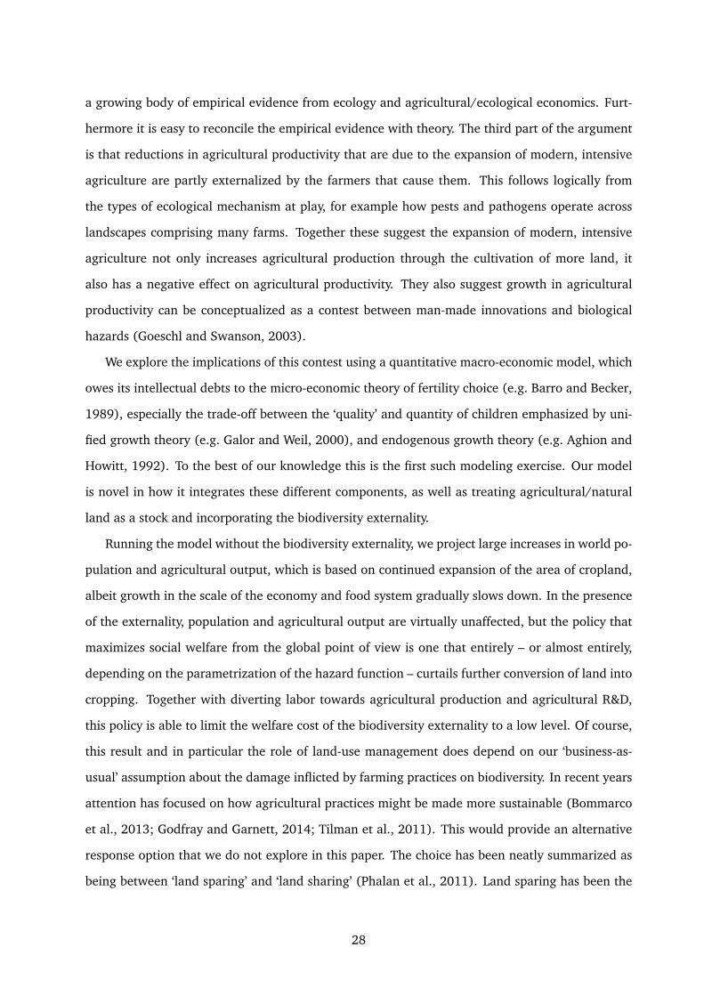
a growing body of empirical evidence from ecology and agricultural/ecological economics. Furt-
hermore it is easy to reconcile the empirical evidence with theory. The third part of the argument
is that reductions in agricultural productivity that are due to the expansion of modern, intensive
agriculture are partly externalized by the farmers that cause them. This follows logically from
the types of ecological mechanism at play, for example how pests and pathogens operate across
landscapes comprising many farms. Together these suggest the expansion of modern, intensive
agriculture not only increases agricultural production through the cultivation of more land, it
also has a negative effect on agricultural productivity. They also suggest growth in agricultural
productivity can be conceptualized as a contest between man-made innovations and biological
hazards (Goeschl and Swanson, 2003).
We explore the implications of this contest using a quantitative macro-economic model, which
owes its intellectual debts to the micro-economic theory of fertility choice (e.g. Barro and Becker,
1989), especially the trade-off between the ‘quality’ and quantity of children emphasized by uni-
fied growth theory (e.g. Galor and Weil, 2000), and endogenous growth theory (e.g. Aghion and
Howitt, 1992). To the best of our knowledge this is the first such modeling exercise. Our model
is novel in how it integrates these different components, as well as treating agricultural/natural
land as a stock and incorporating the biodiversity externality.
Running the model without the biodiversity externality, we project large increases in world po-
pulation and agricultural output, which is based on continued expansion of the area of cropland,
albeit growth in the scale of the economy and food system gradually slows down. In the presence
of the externality, population and agricultural output are virtually unaffected, but the policy that
maximizes social welfare from the global point of view is one that entirely – or almost entirely,
depending on the parametrization of the hazard function – curtails further conversion of land into
cropping. Together with diverting labor towards agricultural production and agricultural R&D,
this policy is able to limit the welfare cost of the biodiversity externality to a low level. Of course,
this result and in particular the role of land-use management does depend on our ‘business-as-
usual’ assumption about the damage inflicted by farming practices on biodiversity. In recent years
attention has focused on how agricultural practices might be made more sustainable (Bommarco
et al., 2013; Godfray and Garnett, 2014; Tilman et al., 2011). This would provide an alternative
response option that we do not explore in this paper. The choice has been neatly summarized as
being between ‘land sparing’ and ‘land sharing’ (Phalan et al., 2011). Land sparing has been the
28
traditional focus of policies and measures to protect natural land, while land sharing is often the
aim of agri-environment schemes, including payments for ecosystem services.
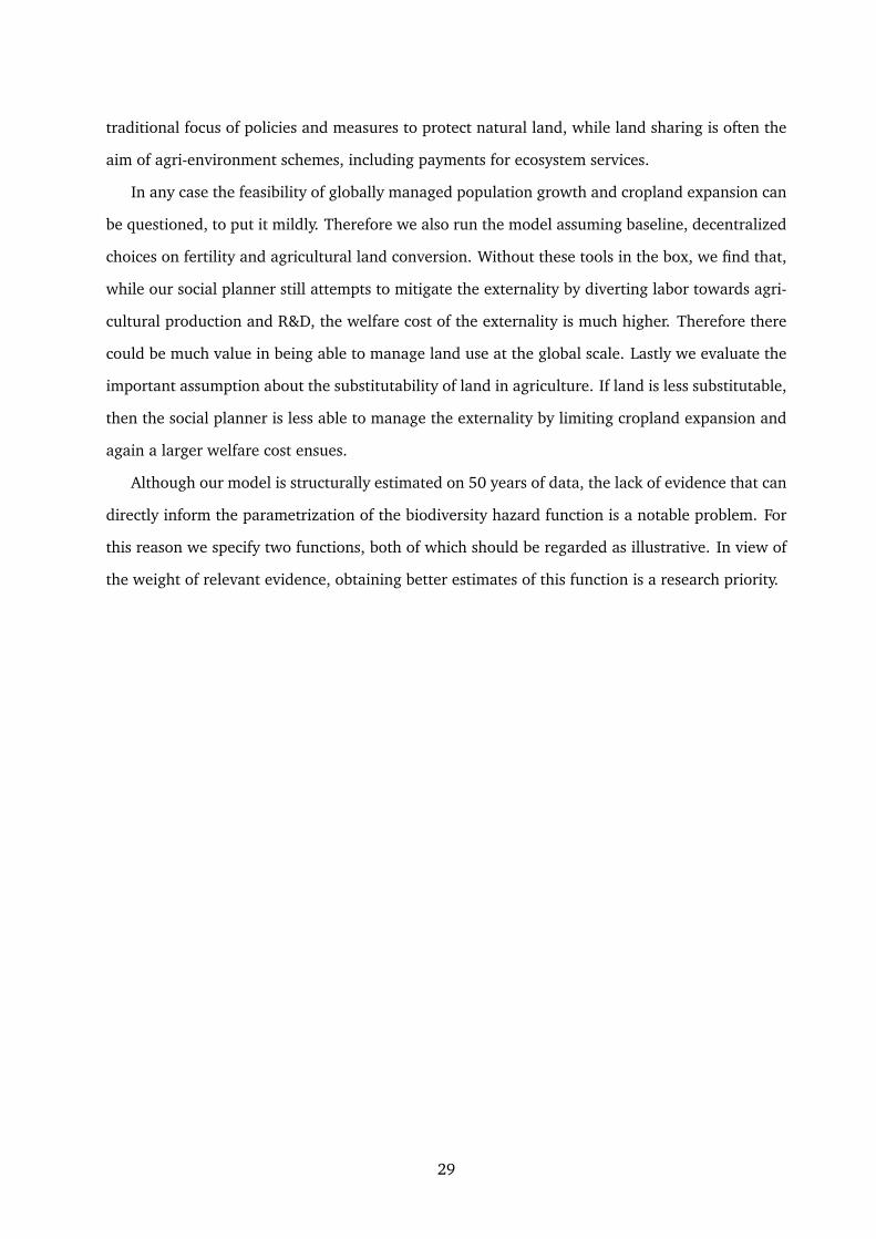
In any case the feasibility of globally managed population growth and cropland expansion can
be questioned, to put it mildly. Therefore we also run the model assuming baseline, decentralized
choices on fertility and agricultural land conversion. Without these tools in the box, we find that,
while our social planner still attempts to mitigate the externality by diverting labor towards agri-
cultural production and R&D, the welfare cost of the externality is much higher. Therefore there
could be much value in being able to manage land use at the global scale. Lastly we evaluate the
important assumption about the substitutability of land in agriculture. If land is less substitutable,
then the social planner is less able to manage the externality by limiting cropland expansion and
again a larger welfare cost ensues.
Although our model is structurally estimated on 50 years of data, the lack of evidence that can
directly inform the parametrization of the biodiversity hazard function is a notable problem. For
this reason we specify two functions, both of which should be regarded as illustrative. In view of
the weight of relevant evidence, obtaining better estimates of this function is a research priority.
29

Appendix A Structural estimation procedure and model fit
As detailed in Lanz et al. (2016), the seven parameters {µmn,ag, χ, ζ, ω, ψ, ε} are estimated using
simulation-based structural methods. The moments we target are taken from observed trajectories
over the period 1960 to 2010 of world GDP (Maddison, 1995; Bolt and van Zanden, 2013), world
population (United Nations, 1999, 2013), crop land area (Goldewijk, 2001; Alexandratos and
Bruinsma, 2012) and sectoral TFP (Martin and Mitra, 2001; Fuglie, 2012).16 In the model these
correspond respectively to Yt,mn + Yt,ag, Nt, Xt, At,mn and At,ag. We target one data point for each
5-year interval, yielding 11 data points for the targeted quantity (55 points in total), and use these
to formulate a minimum distance estimator.
Specifically, the parameters minimize the value of the following expression:
∑k
[∑τ
(Z∗k,τ − Zk,τ )2/∑τ
Zk,τ
], (A1)
where Zk,τ denotes the observed quantity k at time τ and Z∗k,τ is the corresponding value simu-
lated from the model. For each parameter to be estimated from the data, we start by specifying
bounds of a uniform distribution. For elasticity parameters, these bounds are 0.1 and 0.9 and for
the labor productivity parameters we use 0.03 and 0.3. We then solve the model for 10,000 rand-
omly drawn vectors of parameters and evaluate the error between the simulated trajectories and
those observed. By gradually refining the bounds of the distribution, this procedure converges to
the vector of parameters that minimizes goodness-of-fit objective. This procedure converges and
the vector of estimates reported in Table A1.17
16 Data on TFP is derived from TFP growth estimates and are thus subject to some uncertainty. Nevertheless, a robustfinding of the literature is that the growth rate of TFP economy-wide and in agriculture is on average around 1.5-2% per year. To remain conservative about the pace of future technological progress, we assume it declines from1.5 per cent between 1960 and 1980 to 1.2 per cent from 1980 to 2000, and then stays at 1 per cent over the lastdecade.
17 As for other simulation-based estimation procedures involving highly non-linear models, the uniqueness of thesolution cannot be formally proved (see Gourieroux and Monfort, 1996). Our experience with the model suggestshowever that the solution is unique, with no significantly different vector of parameters providing a comparablegoodness-of-fit objective. In other words, estimates reported in Table A1 provide a global solution to the estimationobjective. This is due to the fact that we target a large number of data points for several variables, and thatchanging one parameter will impact trajectories across all variables in the model, which makes the selection criteriafor parameters very demanding.
30

Table A1: Estimation results: Parameters
Parameter Description Estimates
µmn Elasticity of labor in manufacturing R&D 0.581µag Elasticity of labor in agricultural R&D 0.537χ Labor productivity parameter in child-rearing 0.153ζ Elasticity of labor in child-rearing 0.427ω Elasticity of labor productivity in child-rearing w.r.t. technology 0.089ψ Labor productivity in land conversion 0.079ε Elasticity of labor in land-conversion 0.251
The resulting fit of the model is reported in Figure A1, which compares trajectories that were
observed over the period from 1960 to 2010 with the trajectories simulated from the model. As
the charts show, the estimated model provides a very good fit of recent history, and the relative
squared error (A1) across all variables is 3.52 per cent. The size of the error is mainly driven
by the error on output (3.3 per cent), followed by land (0.1 per cent) and population (0.03 per
cent). Figure A1 also reports the growth rate of population, which is not directly targeted by the
estimation procedure, showing that the simulated trajectory closely fits the observed dynamics of
population growth.
31

Figure A1: Estimation of the model 1960 – 2010 (source: Lanz et al., 2016).
0
2
4
6
8
1960 1970 1980 1990 2000 2010
Years
World population in billions (N)
ObservedSimulated
0
0.01
0.02
0.03
1960 1970 1980 1990 2000 2010
Years
Population growth rate (%)
ObservedSimulated
0
0.5
1
1.5
2
1960 1970 1980 1990 2000 2010
Years
Converted agricultural land in billions hectares (X)
ObservedSimulated
0
10
20
30
40
50
60
1960 1970 1980 1990 2000 2010
Years
World GDP in trillions 1990 intl. dollars (Ymn + Yag)
ObservedSimulated
0
1
2
3
1960 1970 1980 1990 2000 2010
Years
Total factor productivity in agriculture (Aag)
ObservedSimulated
0
2
4
6
8
10
12
1960 1970 1980 1990 2000 2010
Years
Total factor productivity in manufacturing (Amn)
ObservedSimulated
32

References
Aghion, P. and P. Howitt (1992) “A model of growth through creative destruction,” Econometrica,60 (2), pp. 323 – 351.
Alexandratos, N. and J. Bruinsma (2012) “World agriculture towards 2030/2050, The 2012 revi-sion.” ESA Working Paper No. 12-03.
Alston, J. M. and P. G. Pardey (2014) “Agriculture in the global economy,” The Journal of EconomicPerspectives, 28, 1, pp. 121–146.
Antràs, P. (2004) “Is the U.S. aggregate production function Cobb-Douglas? New estimates of theelasticity of substitution,” Contributions to Macroeconomics, 4(1), pp. 1–34.
Ashraf, Q. H., A. Lester, and D. Weil (2008) “When does improving health raise GDP?” in D. Ace-moglu, K. Rogoff, and M. Woodford eds. NBER Macroeconomics Annual, pp. 157 – 204: Univer-sity of Chicago Press.
Barro, R. J. and G. S. Becker (1989) “Fertility choice in a model of economic growth,” Econome-trica, 57, pp. 481 – 501.
Barro, R. and X. Sala-i Martin (2004) Economic Growth - Second Edition: Cambridge MA: MITPress.
Baumgärtner, S. (2007) “The insurance value of biodiversity in the provision of ecosystem servi-ces,” Natural Resource Modeling, 20, 1, pp. 87–127.
Beatty, T. K. M. and J. T. LaFrance (2005) “United States demand for food and nutrition in thetwentieth century,” American Journal of Agricultural Economics, 87 (5), pp. 1159 – 1166.
Bolt, J. and J. L. van Zanden (2013) “The first update of the maddison project; re-estimatinggrowth before 1820.” Maddison Project Working Paper 4.
Bommarco, R., D. Kleijn, and S. G. Potts (2013) “Ecological intensification: harnessing ecosystemservices for food security,” Trends in Ecology and Evolution, 28, 4, pp. 230–238.
Bowman, M. S. and D. Zilberman (2013) “Economic factors affecting diversified farming systems,”Ecology and Society, 18, 1, p. 33.
Bretschger, L. (2013) “Population growth and natural resource scarcity: Long-run developmentunder seemingly unfavourable conditions,” Scandinavian Journal of Economics, 115 (3), pp. 722– 755.
Butchart, S. H., M. Walpole, B. Collen, A. van Strien, J. P. Scharlemann, R. E. Almond, J. E.Baillie, B. Bomhard, C. Brown, J. Bruno et al. (2010) “Global biodiversity: indicators of recentdeclines,” Science, 328, 5982, pp. 1164–1168.
Byrd, R., M. E. Hribar, and J. Nocedal (1999) “An interior point method for large scale nonlinearprogramming,” SIAM Journal on Optimization, 9 (4), pp. 877 – 900.
Byrd, R. H., J. Nocedal, and R. A. Waltz (2006) “KNITRO: An integrated package for nonlinearoptimization,” in G. di Pillo and M. Roma eds. Large-Scale Nonlinear Optimization: Springer-Verlag, pp. 35 – 59.
Cardinale, B. J., J. E. Duffy, A. Gonzalez, D. U. Hooper, C. Perrings, P. Venail, A. Narwani, G. M.Mace, D. Tilman, D. A. Wardle, A. P. Kinzig, G. C. Daily, M. Loreau, J. B. Grace, A. Larigauderie,D. S. Srivastava, and S. Naeem (2012) “Biodiversity loss and its impact on humanity,” Nature,486, 7401, pp. 59–67, June.
33

Chu, A., G. Cozzi, and C.-H. Liao (2013) “Endogenous fertility and human capital in a schumpe-terian growth model,” Journal of Population Economics, 26, pp. 181 – 202.
Clarke, L., K. Jiang, K. Akimoto et al. (2014) “Asessing transformation pathways,” in O. Edenhofer,R. Pichs-Madruga, Y. Sokona et al. eds. Climate Change 2014: Mitigation of Climate Change.Contribution of Working Group III to the Fifth Assessment Report of the Intergovernmental Panelon Climate Change, Cambridge, UK and New York, NY, USA: Cambridge University Press.
Dasgupta, P. and G. Heal (1979) Economic Theory and Exhaustible Resources: Cambridge UniversityPress, Cambridge, UK.
Di Falco, S. (2012) “On the value of agricultural biodiversity,” Annu. Rev. Resour. Econ., 4, 1, pp.207–223.
Di Falco, S., M. Bezabih, and M. Yesuf (2010) “Seeds for livelihood: crop biodiversity and foodproduction in ethiopia,” Ecological Economics, 69, 8, pp. 1695–1702.
Dinopoulos, E. and P. Thompson (1998) “Schumpeterian growth without scale effects,” Journal ofEconomic Growth, 3, pp. 313 – 335.
Echevarria, C. (1997) “Changes in sectoral composition associated with economic growth,” Inter-national Economic Review, 38 (2), pp. 431 – 452.
FAO (1996) “The state of the world’s plant genetic resources for food and agriculture,”Technicalreport, Food and Agriculture Organization of the United Nations, Rome.
(2010) “The state of the world’s plant genetic resources for food and agricul-ture,”Technical report, Food and Agriculture Organization of the United Nations, Rome.
Fogel, R. W. (1997) “New findings on secular trends in nutrition and mortality: some implicationsfor population theory,” in M. R. Rosenzweig and O. Stark eds. Handbook of Population andFamily Economics, 1A, Amsterdam: North Holland, Chap. 9, pp. 433–481.
Fuglie, K. O. (2012) “Productivity growth and technology capital in the global agricultural eco-nomy,” in K. O. Fuglie, S. L. Wang, and V. E. Ball eds. Productivity Growth in Agriculture: AnInternational Perspective: Wallingford, U.K.: CAB International, pp. 335 – 368.
Galor, O. and D. N. Weil (2000) “Population, technology, and growth: From malthusian stagnationto the demographic transition and beyond,” American Economic Review, 90 (4), pp. 806 – 828.
Godfray, H. C. J. and T. Garnett (2014) “Food security and sustainable intensification,” Philoso-phical Transactions of the Royal Society B: Biological Sciences, 369, 1639, p. 20120273, April.
Goeschl, T. and T. Swanson (2003) “Pests, plagues, and patents,” Journal of the European EconomicAssociation, 1 (2), pp. 561 – 575.
Goldewijk, K. (2001) “Estimating global land use change over the past 300 years: The hydedatabase,” Global Biogeochemical Cycles, 15 (2), pp. 417 – 433.
Goldin, C. and L. Katz (1998) “The origins of technology-skill complementarity,” Quarterly Journalof Economics, 113, pp. 693 – 732.
Gollin, D. (2002) “Getting income shares right,” Journal of Political Economy, 110 (2), pp. 458 –474.
Gourieroux, C. and A. Monfort (1996) Simulation-Based Econometric Methods: Oxford UniversityPress.
34

Guvenen, F. (2006) “Reconciling conflicting evidence on the elasticity of intertemporal substitu-tion: a macroeconomic perspective,” Journal of Monetary Economics, 53, pp. 1451 – 1472.
Ha, J. and P. Howitt (2007) “Accounting for trends in productivity and R&D: A schumpeteriancritique of semi-endogenous growth theory,” Journal of Money, Credit, and Banking, 39 (4), pp.733 – 774.
Hansen, G. D. and E. C. Prescott (2002) “Malthus to Solow,” American Economic Review, 92 (4),pp. 1204 – 1217.
Heal, G., B. Walker, S. Levin, K. Arrow, P. Dasgupta, G. Daily, P. Ehrlich, K.-G. Maler, N. Kautsky,J. Lubchenco et al. (2004) “Genetic diversity and interdependent crop choices in agriculture,”Resource and Energy Economics, 26, 2, pp. 175–184.
Hertel, T., M. Tsigas, and B. Narayanan (2012) “Chapter 12.a: Primary factor shares,” in B. Nara-yanan, A. Aguiar, and R. McDougall eds. Global Trade, Assistance, and Production: The GTAP 8Data Base: Center for Global Trade Analysis, Purdue University.
Hooper, D. U., E. C. Adair, B. J. Cardinale, J. E. Byrnes, B. A. Hungate, K. L. Matulich, A. Gonzalez,J. E. Duffy, L. Gamfeldt, and M. I. O’Connor (2012) “A global synthesis reveals biodiversity lossas a major driver of ecosystem change,” Nature, 486, 7401, pp. 105–108.
Jones, C. I. (1995) “R&D-based mmodel of economic growth,” The Journal of Political Economy,103 (4), pp. 759 – 784.
(2001) “Was an industrial revolution inevitable? Economic growth over the very longrun,” The B.E. Journal of Macroeconomics, 1 (2), pp. 1–45.
Jones, C. and J. Williams (2000) “Too much of a good thing? The economics of investment inR&D,” Journal of Economic Growth, 5, pp. 65 – 85.
Kawagoe, T., K. Otsuka, and Y. Hayami (1986) “Induced bias of technical change in agriculture:The United States and Japan, 1880-1980,” Journal of Political Economy, 94 (3), pp. 523 – 544.
Khoury, C. K., A. D. Bjorkman, H. Dempewolf, J. Ramirez-Villegas, L. Guarino, A. Jarvis, L. H.Rieseberg, and P. C. Struik (2014) “Increasing homogeneity in global food supplies and theimplications for food security,” Proceedings of the National Academy of Sciences, p. 201313490,March.
Klein Goldewijk, K., A. Beusen, G. van Drecht, and M. de Vos (2011) “The HYDE 3.1 spatiallyexplicit database of human-induced global land-use change over the past 12,000 years,” GlobalEcology and Biogeography, 20, 1, pp. 73–86.
von Lampe, M., D. Willenbockel, H. Ahammad, E. Blanc, Y. Cai, K. Calvin, S. Fujimori, T. Hase-gawa, P. Havlik, E. Heyhoe et al. (2014) “Why do global long-term scenarios for agriculturediffer? an overview of the agmip global economic model intercomparison,” Agricultural Econo-mics, 45, 1, pp. 3–20.
Lanz, B., S. Dietz, and T. Swanson (2016) “Global population growth, technology, and land con-version: A quantitative growth theoretic perspective,” International Economic Review, forthco-ming.
Logan, T. (2009) “The transformation of hunger: The demand for calories past and present,” TheJournal of Economic History, 69 (2), pp. 388 – 408.
Maddison, A. (1995) “Monitoring the world economy 1820 – 1992.” Paris: Organization for Eco-nomic Cooperation and Development.
35

Martin, W. and D. Mitra (2001) “Productivity growth and convergence in agriculture versus ma-nufacturing,” Economic Development and Cultural Change, 49 (2), pp. 403 – 422.
Millennium Ecosystem Assessment (2005) Ecosystems and Human Well-Being: Synthesis, Washing-ton, DC: Island Press.
Mundlak, Y. (2000) Agriculture and economic growth: theory and measurement: Harvard UniversityPress, Cambridge M.A.
Newbold, T., L. N. Hudson, S. L. Hill, S. Contu, I. Lysenko, R. A. Senior, L. Börger, D. J. Bennett,A. Choimes, B. Collen et al. (2015) “Global effects of land use on local terrestrial biodiversity,”Nature, 520, 7545, pp. 45–50.
Ngai, L. R. and C. A. Pissarides (2007) “Structural change in a multisector model of growth,”American Economic Review, 97 (1), pp. 429 — 443.
Nordhaus, W. D. (1992) “An optimal transition path for controlling greenhouse gases,” Science,258, pp. 1315–1315.
Nordhaus, W. D. and J. Boyer (2000) Warming the World: Economic Models of Global Warming:MIT Press (MA).
Oerke, E.-C. (2006) “Crop losses to pests,” Journal of Agricultural Science, 144, pp. 31 – 43.
Omer, A., U. Pascual, and N. P. Russell (2007) “Biodiversity conservation and productivity inintensive agricultural systems,” Journal of Agricultural Economics, 58, 2, pp. 308–329.
Peretto, P. F. (1998) “Technological change and population growth,” Journal of Economic Growth,3, pp. 283 – 311.
Phalan, B., M. Onial, A. Balmford, and R. E. Green (2011) “Reconciling food production andbiodiversity conservation: land sharing and land sparing compared,” Science, 333, 6047, pp.1289–1291.
Poleman, T. T. and L. T. Thomas (1995) “Income and dietary change: international comparisonsusing purchasing-power-parity conversions,” Food Policy, 20, 2, pp. 149–159.
Rausser, G. and A. Small (2000) “Value research leads: Bioprospecting and the conservation ofgenetic resources,” Journal of Political Economy, 108 (1), pp. 173 – 206.
Robinson, S., H. Meijl, D. Willenbockel, H. Valin, S. Fujimori, T. Masui, R. Sands, M. Wise, K. Cal-vin, P. Havlik et al. (2014) “Comparing supply-side specifications in models of global agricultureand the food system,” Agricultural Economics, 45, 1, pp. 21–35.
Savary, S., A. Ficke, J.-N. Aubertot, and C. Hollier (2012) “Crop losses due to diseases and theirimplications for global food production losses and food security,” Food Security, 4, 4, pp. 519–537, December.
Schmitz, C., H. van Meijl, P. Kyle, G. C. Nelson, S. Fujimori, A. Gurgel, P. Havlik, E. Heyhoe, D. M.d’Croz, A. Popp et al. (2014) “Land-use change trajectories up to 2050: insights from a globalagro-economic model comparison,” Agricultural Economics, 45, 1, pp. 69–84.
Sharp, P., H. Strulik, and J. Weisdorf (2012) “The determinants of income in a malthusian equili-brium,” Journal of Development Economics, 97, pp. 112 – 117.
Simpson, R., R. Sedjo, and J. Reid (1996) “Valuing biodiversity for use in pharmaceutical rese-arch,” Journal of Political Economy, 104 (1), pp. 163 – 185.
36

Smale, M., J. Hartell, P. W. Heisey, and B. Senauer (1998) “The contribution of genetic resourcesand diversity to wheat production in the punjab of pakistan,” American Journal of AgriculturalEconomics, 80, 3, pp. 482–493.
Strulik, H. and J. Weisdorf (2008) “Population, food, and knowledge: A simple unified growththeory,” Journal of Economic Growth, 13, pp. 195 – 216.
Subramanian, S. and A. Deaton (1996) “The demand for food and calories,” Journal of PoliticalEconomy, 104 (1), pp. 132 – 162.
Tilman, D. (1999) “The ecological consequences of changes in biodiversity: a search for generalprinciples,” Ecology, 80, 5, pp. 1455–1474.
Tilman, D., C. Balzer, J. Hill, and B. L. Befort (2011) “Global food demand and the sustainableintensification of agriculture,” Proceedings of the National Academy of Sciences, 108, 50, pp.20260–20264.
United Nations (1999) “The world at six billion.” Department of Economic and Social Affairs,Population Division.
(2013) “World population prospects: The 2012 revision.” Department of Economic andSocial Affairs, Population Division, New York.
(2015) World population prospects: the 2015 revision, DVD edition: United Nations, De-partment of Economic and Social Affairs, Population Division.
Vollrath, D. (2011) “The agricultural basis of comparative development,” Journal of EconomicGrowth, 16, pp. 343 – 370.
Weitzman, M. (2000) “Economic profitability versus ecological entropy,” Quarterly Journal of Eco-nomics, 115 (1), pp. 237 – 263.
Wilde, J. (2013) “How substitutable are fixed factors in production? evidence from pre-industrialengland.” Workign paper 0113, University of South Florida, Department of Economics.
World Bank (2016) World Development Indicators, Washington, DC: World Bank.
Young, A. (1998) “Growth without scale effects,” Journal of Political Economy, 106, pp. 41 – 63.
37