The Fascinating World of Landau-Lifshitz-Gilbert · PDF fileLandau-Lifshitz-Gilbert Equation: An Overview ... Then considering the magnetization per unit volume, ... is the simplest

arX

iv:1

101.

1005

v1 [

nlin

.PS]

5 J

an 2

011

The Fascinating World of

Landau-Lifshitz-Gilbert Equation: An

Overview

By M. Lakshmanan

Centre for Nonlinear Dynamics, Department of Physics,Bharathidasan Univeristy, Tiruchirapalli - 620 024, India

The Landau-Lifshitz-Gilbert (LLG) equation is a fascinating nonlinear evolu-tion equation both from mathematical and physical points of view. It is related tothe dynamics of several important physical systems such as ferromagnets, vortexfilaments, moving space curves, etc. and has intimate connections with many of thewell known integrable soliton equations, including nonlinear Schrodinger and sine-Gordon equations. It can admit very many dynamical structures including spinwaves, elliptic function waves, solitons, dromions, vortices, spatio-temporal pat-terns, chaos, etc. depending on the physical and spin dimensions and the nature ofinteractions. An exciting recent development is that the spin torque effect in nano-ferromagnets is described by a generalization of the LLG equation which forms abasic dynamical equation in the field of spintronics. This article will briefly reviewthese developments as a tribute to Robin Bullough who was a great admirer of theLLG equation.

Keywords: LLG Equation, Spin systems, Integrability, Chaos and Patterns

1. Introduction

Spin systems generally refer to ordered magnetic systems. Specifically, spin angu-lar momentum or spin is an intrinsic property associated with quantum particles,which does not have a classical counterpart. Macroscopically, all substances aremagnetic to some extent and every material when placed in a magnetic field ac-quires a magnetic moment or magnetization. In analogy with the relation betweenthe dipole moment of a current loop in a magnetic field and orbital angular momen-tum of a moving electron, one can relate the magnetic moment/magnetization withthe expectation value of the spin angular momentum operator, which one may callsimply as spin. In ferromagnetic materials, the moment of each atom and even theaverage is not zero. These materials are normally made up of domains, which ex-hibit long range ordering that causes the spins of the atomic ions to line up parallelto each other in a domain. The underlying interaction (Hillebrands & Ounadjela2002) originates from a spin-spin exchange interaction that is caused by the overlap-ping of electronic wave functions. Additional interactions which can influence themagnetic structures include magnetocrystalline anisotropy, applied magnetic field,demagnetization field, biquadratic exchange and other weak interactions. Based onphenomenological grounds, by including effectively the above type of interactions,

Article submitted to Royal Society TEX Paper

http://arxiv.org/abs/1101.1005v1

2 Lakshmanan

Landau and Lifshitz (1935) introduced the basic dynamical equation for magneti-

zation or spin ~S(~r, t) in bulk materials, where the effect of relativistic interactionswere also included as a damping term. In 1954, Gilbert (2004) introduced a moreconvincing form for the damping term, based on a Lagrangian approach, and thecombined form is now called the Landau-Lifshitz-Gilbert (LLG) equation, which isa fundamental dynamical system in applied magnetism (Hillebrands & Ounadjela2002; Mattis 1988; Stiles & Miltat 2006).

The LLG equation for the unit spin vector ~S(~r, t), because of the constancyof length, is a highly nonlinear partial differential equation in its original form forbulk materials. Depending on the nature of the spatial dimensions and interactions,it can exhibit a very large variety of nonlinear structures such as spin waves, el-liptic function waves, solitary waves, solitons, lumps, dromions, bifurcations andchaos, spatiotermporal patterns, etc. It exhibits very interesting differential geo-metric properties and has close connections with many integrable soliton and othersystems, for special types of interactions. In the general situations, the system ishighly complex and nonintegrable. Both from physical and mathematical points ofview its analysis is highly challenging but rewarding.

One can also deduce the LLG equation starting from a lattice spin Hamiltonian,by postulating appropriate Poisson brackets, and writing down the correspondingevolution equations and then introducing the Gilbert damping term phenomenolog-ically. Thus we can have LLG equation for a single spin, a lattice of spins and thenthe continuum limit in the form of nonlinear ordinary differential equation(ODE),a system of coupled nonlinear ODEs and a nonlinear partial differential equation,respectively, for the unit spin vector(s). Analysis of the LLG equation for discretespin systems turns out to be even harder than the continuum limit due to the na-ture of nonlinearity. However, apart from exact analytic structures, one can alsorealize the onset of bifurcations, chaos and patterns more easily in discrete cases.Thus the LLG equation turns out to be an all encompassing nonlinear dynamicalsystem.

The LLG equation has also close relationship with several other physical sys-tems, for example motion of a vortex filament, motion of curves and surfaces, σ-models in particle physics, etc. One of the most exciting recent developments is thata simple generalization of the LLG equation also forms the basis of the so calledspin torque effect in nanoferromagnets in the field of spintronics.

With the above developments in mind, in this article we try to present a briefoverview of the different aspects of the LLG equation, concentrating on its nonlineardynamics. Obviously the range of LLG equation is too large and it is too difficultto cover all aspects of it in a brief article and so the presentation will be moresubjective. The structure of the paper will be as follows. In Sec.2, starting from thedynamics of the single spin, extension is made to a lattice of spins and continuumsystems to obtain the LLG equation in all the cases. In Sec.3, we briefly point out thespin torque effect. Sec.4, deals with exact solutions of discrete spin systems, whileSec.5 deals with continuum spin systems in (1+1) dimensions and magnetic solitonsolutions. Sec.5 deals with (2+1) dimensional continuum spin systems. Concludingremarks are made in Sec.6.

Article submitted to Royal Society

Landau-Lifshitz-Gilbert Equation 3

2. Macroscopic Dynamics of Spin Systems and LLGEquation

To start with, in this section we will present a brief account of the phenomenologicalderivation of the Landau-Lifshitz-Gilbert (LLG) equation starting with the equa-tion of motion of a magnetization vector in the presence of an applied magnetic field(Hillebrands & Ounadjela, 2002). Then this analysis is extended to the case of a lat-tice of spins and its continuum limit, including the addition of a phenomenologicaldamping term, to obtain the LLG equation.

(a) Single Spin Dynamics

Consider the dynamics of the spin angular momentum operator ~S of a freeelectron under the action of a time-dependent external magnetic field with theZeeman term given by the Hamiltonian

Hs = −gµB

~

~S. ~B(t), ~B(t) = µ0~H(t), (1)

where g, µB and µ0 are the gyromagnetic ratio, Bohr magneton and permeability invacuum, respectively. Then, from the Schrodinger equation, the expectation valueof the spin operator can be easily shown to satisfy the dynamical equation, usingthe angular momentum commutation relations, as

d

dt< ~S(t) > =

gµB

~< ~S(t) > × ~B(t). (2)

Now let us consider the relation between the classical angular momentum ~L of amoving electron and the dipole moment ~Me of a current loop immersed in a uniformmagnetic field, ~Me =

e2m

~L, where e is the charge and m is the mass of the electron.

Analogously one can define the magnetization ~M = gµB

~< ~S >≡ γ < ~S >, where

γ = gµB

~. Then considering the magnetization per unit volume, ~M , from (2) one

can write the evolution equation for the magnetization as

d ~M

dt= − γ0[ ~M(t)× ~H(t)], (3)

where ~B = µ0~H and γ0 = µ0γ.

From (3) it is obvious that ~M. ~M = constant and ~M. ~H = constant. Conse-quently the magnitude of the magnetization vector remains constant in time, whileit precesses around the magnetic field ~H making a constant angle with it. Definingthe unit magnetization vector

~S(t) =~M(t)

| ~M(t)|, ~S2 = 1, ~S = (Sx, Sy, Sz), (4)

which we will call simply as spin hereafter, one can write down the spin equationof motion as (Hillebrands & Ounadjela 2002)

d~S(t)

dt= − γ0[~S(t)× ~H(t)], ~H = (Hx, Hy, Hz) (5)


4 Lakshmanan

(a)

H

/ dt

(b)

H

x / dt

/ dt

S

S S

Sd

SdSd

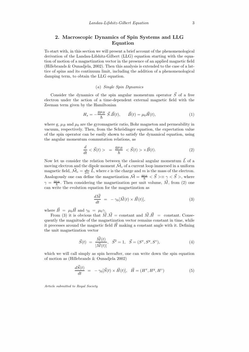
Figure 1. Evolution of a single spin (a) in the presence of a magnetic field and (b) whendamping is included.

and the evolution of the spin can be schematically represented as in Fig. 1(a).It is well known that experimental hysteresis curves of ferromagnetic substances

clearly show that beyond certain critical values of the applied magnetic field, themagnetization saturates, becomes uniform and aligns parallel to the magnetic field.In order to incorporate this experimental fact, from phenomenological grounds onecan add a damping term suggested by Gilbert (2004) so that the equation of motioncan be written as

d~S(t)

dt= − γ0[~S(t)× ~H(t)] + λγ0

[

~S ×d~S

dt

]

, λ ≪ 1(damping parameter). (6)

On substituting the expression (6) again for d~Sdt

in the third term of (6), it can berewritten as

(1 + λ2γ0)d~S

dt= − γ0[~S × ~H(t)]− λγ0 ~S × [~S × ~H(t)].

After a suitable rescaling of t, Eq.(6) can be rewritten as

d~S

dt= (~S × ~H(t)) + λ~S × [~S × ~H(t)]

= ~S × ~Heff . (7)

Here the effective field including damping is

~Heff = ~H(t) + λ[~S × ~H ]. (8)

The effect of damping is shown in Fig 1(b). Note that in Eq.(7) again the constancyof the length of the spin is maintained. Eq.(7) is the simplest form of Landau-Lifshitz-Gilbert equation, which represents the dynamics of a single spin in thepresence of an applied magnetic field ~H(t).

(b) Dynamics of Lattice of Spins and Continuum Case

The above phenomenological analysis can be easily extended to a lattice ofspins representing a ferromagnetic material. For simplicity, considering an one di-mensional lattice of N spins with nearest neighbour interactions, onsite anisotropy,



demagnetizing field, applied magnetic field, etc., the dynamics of the ith spin canbe written down in analogy with the single spin as the LLG equation,

d~Si

dt= ~Si × ~Heff , i = 1, 2, ......N (9)

where

~Heff = (~Si+1 + ~Si−1 +ASxi ~nx +BS

yi ~ny + CSz

i ~nz + ~H(t) + ......)

− λ~Si+1 + ~Si−1 +ASxi ~nx +BS

yi ~ny + CSz

i ~nz + ~H(t) + ...... × ~Si (10)

Here A,B,C are anisotropy parameters, and ~nx, ~ny, ~nz are unit vectors along thex, y and z directions, respectively. One can include other types of interactions likebiquadratic exchange, spin phonon coupling, dipole interactions, etc. Also Eq.(9)can be generalized to the case of square and cubic lattices as well, where the indexi has to be replaced by the appropriate lattice vector ~i.

In the long wavelength and low temperature limit, that is in the continuumlimit, one can write

~S~i(t) = ~S(~r, t), ~r = (x, y, z),

~S~i+~1 +~S~i−~1 = ~S(~r, t) + ~a.~∇~S +

a2

2∇2~S + higher orders, (11)

(~a: lattice vector) so that the LLG equation takes the form of a vector nonlinearpartial differential equation (as ~a → ~0),

∂ ~S(~r, t)

∂t=~S ×

[

∇2~S +ASx~nx +BSy~ny + CSz~nz + ~H(t) + ....]

+ λ[

∇2~S +ASx~nx +BSy~ny + CSz~nz + ~H(t) + ....

× ~S(~r, t)]

,

=~S × ~Heff (12)

~S(~r, t) =(Sx(~r, t), Sy(~r, t), Sz(~r, t)), ~S2 = 1. (13)

In fact, Eq.(12) was deduced from phenomenological grounds for bulk magneticmaterials by Landau and Lifshitz originally in 1935.

(c) Hamiltonian Structure of the LLG Equation in the Absence of Damping

The dynamical equations for the lattice of spins (9) in one dimension (as well asin higher dimensions) posses a Hamiltonian structure in the absence of damping.

Defining the spin Hamiltonian

Hs = −∑

i,j

~Si.~Si+1 +A(Sxi )

2 +B(Syi )

2 + C(Szi )

2 + µ( ~H(t).~Si) + ..... (14)

and the spin Poisson brackets between any two functions of spin A and B as

A,B =

3∑

α,β,γ=1

∈αβγ

∂A

∂Sα

∂B

∂SβSγ , (15)


6 Lakshmanan

one can obtain the evolution equation (9) for λ = 0 from d~Si

dt= ~Si, Hs. Here ∈αβγ

is the Levi-Civitta tensor. Similarly for the continuum case, one can define the spinHamiltonian density

Hs =1

2[(∇~S)2 +A(Sx)2 +B(Sy)2 + C(Sz)2 + ( ~H.~S) +Hdemag + ......] (16)

along with the Poisson bracket relation

Sα(~r, t), Sβ(~r′

, t′

)

=∈αβγ Sγδ(~r − ~r′

, t− t′

), (17)

and deduce the spin field evolution equation (12) for λ = 0.Defining the energy as

E =1

2

∫

d3r[(∇~S)2 +A(Sx)2 +B(Sy)2 + C(Sz)2 + ~H.~S + ....] (18)

one can easily check that

dE

dt= −λ

∫

|~St|2d3r.

Then when λ > 0, the system is dissipative, while for λ = 0 the system is conser-vative.

3. Spin Torque Effect and the Generalized LLG Equation

Consider the dynamics of spin in a nanoferromagnetic film under the action of aspin current (Stiles & Miltat, 2006; Bertotti et al. 2009). In recent times it hasbeen realized that if the current is spin polarized, the transfer of a strong currentacross the film results in a transfer of spin angular momentum to the atoms ofthe film. This is called spin torque effect and forms one of the basic ideas of theemerging field of spintronics. The typical set up of the nanospin valve pillar consistsof two ferromagnetic layers, one a long ferromagnetic pinned layer, and the secondone is of a much smaller length, separated by a spacer conductor layer [6], all ofwhich are nanosized. The pinned layer acts as a reservoir of spin polarized currentwhich on passing through the conductor and on the ferromagnetic layer inducesan effective torque on the spin magnetization in the ferromagnetic film, leading torapid switching of the spin direction of the film. Interestingly, from a semiclassicalpoint of view, the spin transfer torque effect is described by a generalized versionof the LLG equation (12), as shown by Berger (1996), and by Slonczewski (1996),in 1996. Its form reads

∂~S

∂t= ~S × [ ~Heff + ~S ×~j], ~S = (Sx, Sy, Sz), ~S2 = 1 (19)

where the spin current term

~j =a.~SP

f(P )(3 + ~S.~SP ), f(P ) =

(1 + P 3)

4P3

2

. (20)



Here ~SP is the pinned direction of the polarized spin current which is normally takenas perpendicular to the direction of flow of current, a is a constant factor relatedto the strength of the spin current and f(P ) is the polarization factor deducedby Slonczewski (1996) from semiclassical arguments. From an experimental pointof view valid for many ferromagneic materials it is argued that it is sufficient toapproximate the spin current term simply as

~j = a~Sp (21)

so that LLG equation for the spin torque effect can be effectively written down as

∂~S

∂t= ~S × [ ~Heff + a~S × ~Sp], (22)

where

~Heff = (∇2~S +ASx~i+BSy~j + CSz~k + ~Hdemag + ~H(t) + .....)− λ~S ×∂~S

∂t. (23)

Note that in the present case, using the energy expression (18), one can prove that

dE

dt=

∫

[−λ|St|2 + a(~St × ~S).~Sp]d

3r. (24)

This implies that energy is not necessarily decreasing along trajectories. Conse-quently, many interesting dynamical features of spin can be expected to arise inthe presence of the spin current term.

In order to realize these effects more transparently, let us rewrite the generalizedLLG equation(22) in terms of the complex stereographic variable ω(~r, t)(Lakshmanan& Nakumara, 1984) as

ω =Sx + iSy

(1 + Sz), (25a)

Sx =ω + ω∗

(1 + ωω∗), Sy =

1

i

(ω − ω∗)

(1 + ωω∗), Sz =

(1 − ωω∗)

(1 + ωω∗)(25b)

so that Eq.(20) can be rewritten (for simplicity ~Hdemag = 0 )

i(1− iλ)ωt +∇2ω −2ω∗(∇ω)2

(1 + ωω∗)+

A

2

(1 − ω2)(ω + ω∗)

(1 + ωω∗)

+B

2

(1 + ω2)(ω − ω∗)

(1 + ωω∗)− C(

1− ωω∗

1 + ωω∗)ω

+1

2(Hx − ijx)(1− ω2) +

1

2i(Hy + ijy)(1 + ω2)− (Hz + ijz)ω = 0, (26)

where ~j = a~Sp, ωt = (∂ω∂t

).

It is clear from Eq.(26) that the effect of the spin current term ~j is simply to

change the magnetic field ~H = (Hx, Hy, Hz) as (Hx − ijx, Hy + ijy, Hz + ijz).Consequently the effect of the spin current is effectively equivalent to a magnetic


8 Lakshmanan

field, though complex. The consequence is that the spin current can do the functionof the magnetic field perhaps in a more efficient way because of the imaginary term.

To see this in a simple situation, let us consider the case of a homogeneousferromagnetic film so that there is no spatial variation and the anisotropy anddemagnetizing fields are absent, that is we have (Murugesh & Lakshmanan, 2009a)

(1− iλ)ωt = −(a− iHz)ω. (27)

Then on integration one gets

ω(t) = ω(0)exp[−(a− iHz)t

(1− iλ)]

= ω(0)exp

[

−(a+ λHz)t

(1 + |λ|2)

]

exp

[

−i(aλ−Hz)t

(1 + |λ|2)

]

. (28)

Obviously the first exponent describes a relaxation or switching of the spin, whilethe second term describes a precession. From the first exponent in (28), it is clear

that the time scale of switching is given by 1+|λ|2

(a+λHz) . Here λ is small which implies

that the spin torque term is more effective in switching the magnetization vector.Furthermore letting Hz term to become zero, we note that in the presence of damp-ing term the spin transfer produces the dual effect of precession and dissipation.

In Fig.2, we point out clearly how the effect of spin current increases the rate ofswitching of the spin even in the presence of anisotropy. Further, one can show thatinteresting bifurcation scenerio, including period doubling bifurcations to chaoticbehaviour, occurs on using a periodically varying applied magnetic field in thepresence of a constant magnetic field and constant spin current (Murugesh & Lak-shmanan, 2009a). Though a periodically varying spin current can also lead to sucha bifurcations-chaos scenerio (Yang et al. 2007), we believe the technique of apply-ing a periodic magnetic field in the presence of constant spin current is much morefeasible experimentally. To realize this one can take (Murugesh & Lakshmanan,2009b)

~Heff = κ(~S.~e‖)~e‖ + ~Hdemag + ~H(t), (29)

where κ is the anisotropy parameter and ~e‖ is the unit vector along the anisotropyaxis and

~Hdemag = −4π(N1Sx~i+N2S

y~j +N3Sz~k). (30)

Choosing

~H(t) = (0, 0, Hz), ~e‖ = (sinθ‖cosφ‖, sinθ‖sinφ‖, cosθ‖), (31)

the LLG equation in stereographic variable can be written down(in the absence ofexchange term) as (Murugesh & Lakshmanan, 2009a,b)

(1− iλ)ωt =− γ(a− iHz)ω + iS‖κγ

[

cosθ‖ω −1

2sinθ‖

(

eiφ‖ − ω2e−iφ‖)

]

−i4πγ

(1 + |ω|2)

[

N3(1− |ω|2)ω −N1

2(1 − ω2 − |ω|2)ω

−N2

2(1 + ω2 − |ω|2)ω −

(

N1 −N2

2

)

ω

]

, (32)



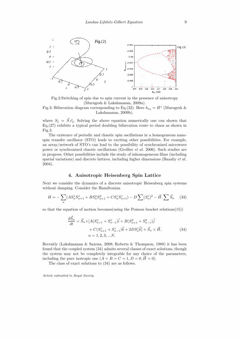
Fig.2:Switching of spin due to spin current in the presence of anisotropy(Murugesh & Lakshmanan, 2009a).

Fig.3: Bifurcation diagram corresponding to Eq.(32). Here ha3= Hz (Murugesh &

Lakshmanan, 2009b).

where S‖ = ~S.~e‖. Solving the above equation numerically one can shown thatEq.(27) exhibits a typical period doubling bifurcation route to chaos as shown inFig.3.

The existence of periodic and chaotic spin oscillations in a homogeneous nano-spin transfer oscillator (STO) leads to exciting other possibilities. For example,an array/network of STO’s can lead to the possibility of synchronized microwavepower or synchronized chaotic oscillations (Grollier et al. 2006). Such studies arein progress. Other possibilities include the study of inhomogeneous films (includingspatial variations) and discrete lattices, including higher dimensions (Bazaliy et al.2004).

4. Anisotropic Heisenberg Spin Lattice

Next we consider the dynamics of a discrete anisotropic Heisenberg spin systemswithout damping. Consider the Hamiltonian

H = −∑

n

(ASxnS

xn+1 +BSy

nSyn+1 + CSz

nSzn+1)−D

∑

(Szn)

2 − ~H.∑

~Sn (33)

so that the equation of motion becomes(using the Poisson bracket relations(15))

d~Sn

dt= ~Sn×[A(Sx

n+1 + Sxn−1)~i +B(Sy

n+1 + Syn−1)~j

+ C(Szn+1 + Sz

n−1)~k + 2DSz

n~k] + ~Sn × ~H, (34)

n = 1, 2, 3, ...N.

Recently (Lakshmanan & Saxena, 2008; Roberts & Thompson, 1988) it has beenfound that the coupled system (34) admits several classes of exact solutions, thoughthe system may not be completely integrable for any choice of the parameters,including the pure isotropic one (A = B = C = 1, D = 0, ~H = 0).

The class of exact solutions to (34) are as follows.


10 Lakshmanan

(a) Spatially homogeneous time dependent solution:

Sxn = −

√

1− γ2k′2 sn(ωt+ δ, k), (35a)

Syn =

√

1− γ2 cn(ωt+ δ, k), (35b)

Szn = γ dn(ωt+ δ, k), (35c)

where the frequency

ω = 2γ√

(B − C)(A− C), k2 =1− γ2

γ2

(B −A)

(A− C)(B > A > C). (35d)

Here γ and δ are arbitrary parameter and k is the modulus of the Jacobian ellipticfunctions.

(b) Spatially oscillatory time periodic solutions

Sxn = (−1)n+1

√

1− γ2k′2 sn(ωt+ δ, k), (36a)

Syn = (−1)n

√

1− γ2 cn(ωt+ δ, k), (36b)

Szn = γ dn(ωt+ δ, k), (36c)

where

ω = 2γ√

(A+ C)(B + C), k2 =1− γ2

γ2

(B −A)

(A+ C). (36d)

This solution corresponds to a nonlinear magnon.

(c) Linear magnon solutions

In the uniaxial anisotropic case A = B < C, the linear magnon solution is

Sxn =

√

1− γ2 sin(pn− ωt+ δ), (37a)

Syn =

√

1− γ2 cos(pn− ωt+ δ), (37b)

Szn = γ (37c)

with the dispersion relation

ω = 2γ(C −A cos p). (37d)

(d) Nonplanar static structures for XYZ and XYY models

In this case we have the periodic structures

Sxn =

√

1− γ2k′2 sn(pn+ δ, k), (38a)

Syn =

√

1− γ2 cn(pn+ δ, k), (38b)

Szn = γ dn(pn+ δ, k), (38c)



where

k2 =A2 −B2

A2 − C2, dn(p, k) =

B

A. (38d)

In the limiting case k = 1, one can obtain the localized single soliton (solitary wave)solution

Sxn = tanh(pn+ δ), Sy

n =√

1− γ2 sech(pn+ δ), Szn = γ sech(pn+ δ). (39)

(e) Planar (XY) Case:

Case(i) : Sxn = sn(pn+ δ, k), Sy

n = cn(pn+ δ, k), Szn = 0, (40)

where dn(p, k) = BA. In the limiting case, k = 1, we have the solitary wave solution

Sxn = tanh(pn+ δ, k), Sy

n = sech(pn+ δ), Szn = 0. (41)

Case(ii) : Sxn = k sn(pn+ δ, k), Sz

n = dn(pn+ δ, k), Syn = 0, (42)

where cn(p, k) = CA. In the limit k = 1, we have

Sxn = tanh(pn+ δ), Sy

n = 0, Szn = sech(pn+ δ). (43)

(f ) Nonplanar XYY Structures:

We have

Sxn = cn(pn+ δ, k), Sy

n = γ sn(pn+ δ, k), Szn =

√

1− γ2 sn(pn+ δ, k), (44)

where dn(p, k) = AB. In the limiting case, we have the domain wall structure

Sxn = sech(pn+ δ), Sy

n = γ tanh(pn+ δ), Szn =

√

1− γ2 tanh(pn+ δ). (45)

In all the above cases one can evaluate the energies associated with the differentstructures and their linear stability properties. For details, one may refer to (Lak-shmanan & Saxena, 2008).

(g) Solutions in the presence of onsite anisotropy and constant external magneticfield

(i) Onsite anisotropy, D 6= 0, H = 0, A,B,C 6= 0 :

All the three types of solutions (35), (36) and (37) exist here also, except thatthe parameter C has to be replaced by (C −D) in each of these equations on theirright hand sides.


12 Lakshmanan

(ii) Constant external field case, ~H = (Hx, 0, 0), B = C 6= A, D = 0.

An exact solution is

Sxn = sn(pn+ δ, k), (46a)

Syn = sin(ωt+ γ) cn(pn+ δ, k), (46b)

Szn = cos(ωt+ γ) cn(pn+ δ, k), (46c)

where dn(p, k) = CA, and ω = Hx.

One can study the linear stability of static solutions and investigate the existenceof the so called Peierls-Nabarro barrier, that is whether the total lattice energydepends on the location of the soliton or not, for details see (Lakshmanan & Saxena,2008).

(h) Integrability of the static case

Granovskii and Zhedanov(1986) have shown that the static case of the pureanisotropic system

~Sn ×[

A(Sxn+1 + Sx

n−1) +B(Syn+1 + S

yn−1) + C(Sz

n+1 + Szn−1)

]

= 0 (47)

is equivalent to a discretized version of the Schrodinger equation with two levelBargmann type potential or a discrete analog of Neumann system (Veselov, 1987)and is integrable.

(i) Ishimori spin chain:

There exists a mathematically interesting spin chain which is completely inte-grable and which was introduced by Ishimori (1982). Starting with a Hamiltonian

H = −log(1 +∑

~Sn.Sn+1), the spin equation becomes

Sn = ~Sn ×

[

~Sn+1

1 + ~Sn.~Sn+1

+~Sn−1

1 + ~Sn.~Sn−1

]

(48)

It admits a Lax pair and so is completely integrable. However, no other realistic spinsystem is known to be completely integrable. It is interesting to note that Eq.(48)also leads to an integrable reversible map. Assuming a simple time dependence,

~Sn(t) = (cosφncosωt, cosφnsinωt, sinφn), (49)

Quispel, Robert and Thompson (1988) have shown that Eq.(48) reduces to theintegrable map

xn+1 =[2x3n + ωx2

n + 2xn − ω − xn−1(−x4n − ωx3

n + ωxn + 1)]

× [−x4n − ωx3

n + ωxn + 1− xn−1(ωx4n − 2x3

n − ωx2n − 2xn)]

−1. (50)

Finally, it is also of interest to note that one can prove the existence of localizedexcitations, using implicit function theorem, of tilted magnetization or discretebreathers (so called nonlinear localized modes) in a Heisenberg spin chain with easy-plane anisotropy (Zolotaryuk et al. 2001). It is obvious that there is much scope



for detailed study of the discrete spin system to understand magnetic properties,particularly by including Gilbert damping term and also the spin current, see forexample a recent study on the existence of vortices and their switching of polarityon the application of spin current (Sheka et al. 2007).

5. Continuum Spin Systems in (1+1) Dimensions

The continuum case of the LLG equation is a fascinating nonlinear dynamicalsystem. It has close connection with several integrable soliton systems in the absenceof damping in (1+1) dimensions and possesses interesting geometric connections.Then damping can be treated as a perturbation. In the (2+1) dimensional case novelstructures like line soliton, instanton, dromion, spatiotemporal patterns, vortices,etc. can arise. They have both interesting mathematical and physical significance.We will briefly review some of these features and indicate a few of the challengingtasks needing attention.

(a) Isotropic Heisenberg Spin System in (1+1) Dimensions

Considering the (1+1) dimensional Heisenberg ferromagnetic spin system withnearest neighbour interaction, the spin evolution equation without damping can bewritten as (after suitable scaling)

~St = ~S × ~Sxx, ~S = (Sx, Sy, Sz), ~S2 = 1. (51)

In Eq.(51) and in the following suffix stands for differentiation with respect to thatvariable.

We now map the spin system (Lakshmanan et al. 1976) onto a space curve (inspin space) defined by the Serret-Frenet equations,

~eix = ~D × ~ei, ~D = τ~e1 + κ~e3, ~ei.~ei = 1, i = 1, 2, 3, (52)

where the triad of orthonormal unit vectors ~e1, ~e2, ~e3 are the tangent, normal andbinormal vectors, respectively, and x is the arclength. Here κ and τ are the curvatureand torsion of the curve, respectively, so that κ2 = ~e1x.~e1x (energy density), κ2τ =~e1.(~e1x × ~e1xx) is the current density.

Identifying the spin vector ~S(x, t) of Eq.(51) with the unit tangent vector ~e1,from (51) and (52), one can write down the evolution of the trihedral as

~eit = ~Ω× ~ei, ~Ω = (ω1, ω2, ω3) =(κxx

κ− τ2,−κx,−κτ

)

. (53)

Then the compatibility (~ei)xt = (~ei)tx, i = 1,2,3, leads to the evolution equation

κt = −2κxτ − κτx, (54a)

τt = (κxx

κ− τ2)x + κκx, (54b)

which can be rewritten equivalently (Lakshmanan, 1977) as the ubiquitous nonlin-ear Schrodinger (NLS) equation,

iqt + qxx + 2|q|2q = 0, (55)


14 Lakshmanan

through the complex transformation

q =1

2κ exp

[

i

∫ +∞

x

τ dx′

]

, (56)

and thereby proving the complete integrability of Eq.(51).Zakharow and Takhtajan (1979) have also shown that this equivalence between

the (1+1) dimensional isotropic spin chain and the NLS equation is a gauge equiv-alence. To realize this, one can write down the Lax representation of the isotropicsystem (51) as (Takhtajan, 1977)

φ1x = U1(x, t, λ)φ1, φ1t = V1(x, t, λ)φ1, (57)

where the (2 × 2) matrices U1 = iλS, V1 = λSSx + 2iλ2S, S =

(

Sz S−

S+ −Sz

)

,

S± = Sx± iSy. Then considering the Lax representation of the NLS equation (55),

φ2x = U2φ2, φ2t = V2φ2, (58)

where U2 = (A0 + λA1), V2 = (B0 + λB1 + λ2B2),

A0 =

(

0 q∗

−q 0

)

, A1 = iσ3, B0 = 1i

(

|q2| q∗xqx −|q|2

)

,

B1 = 2A0, B2 = 2A1, σi’s are the Pauli matrices, one can show that withthe gauge transformation

φ1 = g−1φ2, S = g−1σ3g, (59)

(57) follows from (58) and so the systems (51) and (55) are gauge equivalent.The one soliton solution of the Sz component can be written down as

Sz(x, t) = 1−2ξ

ξ2 + η2sech2ξ(x− 2ηt− x0), ξ, η, x0 : constants (60)

Similarly the other components Sx and Sy can be written down and the N-solitonsolution deduced.

(b) Isotropic chain with Gilbert damping

The LLG equation for the isotropic case is

~St = ~S × ~Sxx + λ[~Sxx − (~S.~Sxx)~S]. (61)

The unit spin vector ~S(x, t) can be again mapped onto the unit tangent vector ~e1of the space curve and proceeding as before (Daniel & Lakshmanan, 1983) one canobtain the equivalent damped nonlinear Schrodinger equation,

iqt + qxx + 2|q|2q = iλ[qxx − 2q

∫ x

−∞

(qq∗x′ − q∗qx′ )dx

′

], (62)

where again q is defined by Eq.(55) with curvature and torsion defined as before.Treating the damping terms proportional to λ as a perturbation, one can analysethe effect of damping on the soliton structure.



(c) Inhomogeneous Heisenberg Spin System

Considering the inhomogeneous spin system, corresponding to spatially depen-dent exchange interaction,

~St = (γ2 + µ2x)~S × ~Sxx + µ2~S × ~Sx − (γ1 + µ1x)~Sx, (63)

where γ1, γ2, µ1 and µ2 are constants, again using the space curve formalism,the present author and Robin Bullough (Lakshmanan & Robin Bullough, 1980)showed the geometrical/gauge equivalence of Eq.(63) with the linearly x-dependentnonlocal NLS equation,

iqt = iµ1q + i(γ1 + µ1x)qx

+ (γ2 + µ2x)(qxx + 2|q|2q) + 2µ2(qx + q

∫ x

−∞

|q|2dx′

) = 0. (64)

It was also shown in (Lakshmanan & Bullough, 1980) that the both the systems(63) and (64) are completely integrable and the eigenvalues of the associated linearproblems are time dependent.

(d) n-dimensional Spherically Symmetric (radial) Spin System

The spherically symmetric n -dimensional Heisenberg spin system (Daniel et al.1994)

~St(r, t) = ~S ×

[

~Srr +(n− 1)

r~Sr

]

, (65)

~S2(r, t) = 1, ~S = (Sx, Sy, Sz), r2 = r21 + r22 + ...+ r2n, 0 ≤ r < ∞,

can be also mapped onto the space curve and can be shown to be equivalent to thegeneralized radial nonlinear Schrodinger equation,

iqt + qrr +(n− 1)

rqr =

(

n− 1

r2− 2|q|2 − 4(n− 1)

∫ r

0

|q|2

r′ dr

′

)

q. (66)

It has been shown that only the cases n = 1 and n = 2 are completely integrablesoliton systems (Mikhailov & Yaremchuk, 1982; Porsezian & Lakshmanan, 1991)with associated Lax pairs.

(e) Anisotropic Heisenberg spin systems

It is not only the isotropic spin system which is integrable, even certain anisotropiccases are integrable. Particularly the uniaxial anisotropic chain

~St = ~S × [~Sxx + 2A Sz~nz + ~H], ~nz = (0, 0, 1) (67)

is gauge equivalent to the NLS equation (Nakamura & Sasada, 1982) in the case

of longitudinal field ~H = (0, 0, Hz) and is completely integrable. Similarly thebianisotropic system

~St = ~S × ~J ~Sxx, ~J = diag(J1, J2, J3), J1 6= J2 6= J3, (68)


16 Lakshmanan

possesses a Lax pair and is integrable (Sklyanin, 1979). On the other hand theanisotropic spin chain in the case of transverse magnetic field, H = (Hx, 0, 0),is nonintegrable and can exhibit spatiotemporal chaotic structures (Daniel et al.1992).

Apart from the above spin systems in (1+1) dimensions, there exists a few otherinteresting cases which are also completely integrable. For example, the isotropicbiquadratic Heisenberg spin system,

~St = ~S ×

[

Sxx + γ

~Sxxxx −5

2(~S.~Sxx)Sxx −

5

3(~S.~Sxxx)~Sx

]

(69)

is an integrable soliton system (Porsezian et al. 1992) and is equivalent to a fourthorder generalized nonlinear Schrodinger equation,

iqt + qxx + 2|q|2 + γ[

qxxxx + 8|q|2qxx + 2q2q∗xx + 4q|qx|2 + 6q∗q2x + 6|q|4q

]

= 0.(70)

Similarly the SO(3) invariant deformed Heisenberg spin equation,

~St = ~S × ~Sxx + α~Sx(~Sx)2, (71)

is geometrically and gauge equivalent to a derivative NLS equation (Porsezian et al.1987),

iqt + qxx +1

2|q|2q − iα(|q|2q)x = 0. (72)

There also exist several studies which maps the LLG equation in different limitsto sine-Gordon equation (planar system), Korteweg-de Vries (KdV), mKdV andother equations, depending upon the nature of the interactions. For details see forexample (Mikeska & Steiner, 1991; Daniel & Kavitha, 2002).

6. Continuum Spin Systems in Higher Dimensions

The LLG equation in higher spatial dimensions, though physically most important,is mathematically highly challenging. Unlike the (1+1) dimensional case, even inthe absence of damping, very few exact results are available in (2+1) or (3+1)dimensions. We briefly point out the progress and challenges.

(a) Nonintegrability of the Isotropic Heisenberg Spin Systems

The (2+1) dimensional isotropic spin system

~St = ~S ×(

~Sxx + ~Syy

)

, ~S = (Sx, Sy, Sz), ~S2 = 1, (73)

under stereographic projection, see Eq.(25), becomes (Lakshmanan & Daniel, 1981)

(1 + ωω∗)[iωt + ωxx + ωyy]− 2ω∗(ω2x + ω2

y) = 0. (74)



It has been shown (Senthilkumar et al. 2006) to be of non-Painleve nature. Thesolutions admit logarithmic type singular manifolds and so the system (73) is non-integrable. It can admit special types of spin wave solutions, plane solitons, ax-isymmetric solutions, etc. (Lakshmanan & Daniel, 1981). Interestingly, the staticcase

ωxx + ωyy =2ω∗

(1 + ωω∗)2(ω2

x + ω2y) (75)

admits instanton solutions of the form

ω = (x1 + ix2)m, Sz =

1− (x21 + x2

2)m

1 + (x21 + x2

2)m, m = 0, 1, 2, .... (76)

with a finite energy (Belavin & Polyakov, 1975; Daniel & Lakshmanan, 1983). Fi-nally, very little information is available to date on the (3+1) dimensional isotropicspin systems (Guo & Ding, 2008)

(b) Integrable (2+1) Dimensional Spin Models

While the LLG equation even in the isotropic case is nonintegrable in higherdimensions, there exists a couple of integrable spin models of generalized LLGequation without damping in (2+1) dimensions. These include the Ishimori equa-tion (Ishimori, 1984) and Myrzakulov equation (Lakshmanan et al. 1998), whereinteraction with an additional scalar field is included.

(i) Ishimori equation:

~St = ~S × (~Sxx + ~Syy) + ux~Sy + uy

~Sx, (77a)

uxx − σ2uyy = −2σ2~S.(~Sx × ~Sy), σ2 = ±1. (77b)

Eq.(77) admits a Lax pair and is solvable by inverse scattering transform (d-bar)method (Konopelchenko & Matkarimov, 1989). It is geometrically and gauge equiv-alent to Davey-Stewartson equation and admits exponentially localized dromion so-lutions, besides the line solitons and algebraically decaying lump soliton solutions.It is interesting to note that here one can map the spin onto a moving surfaceinstead of a moving curve (Lakshmanan et al. 1998).

(ii) Myszakulov equation I(Lakshmanan et al. 1998)

The modified spin equation

~St =(

~S × ~Sy + u~S)

x, ux = −~S.(~Sx × ~Sy) (78)

can be shown to be geometrically and gauge equivalent to the Calogero-Zakharov-Strachan equation

iqt = qxy + V q, Vx = 2(|q|2)y (79)


18 Lakshmanan

and is integrable. It again admits line solitons, dromions and lumps.However from a physical point of view it will be extremely valuable if exact

analytic structures of the LLG equation in higher spatial dimensions are obtainedand the so called wave collapse problem (Sulem & Sulem, 1999) is investigated infuller detail.

(c) Spin Wave Instabilities and Spatio-temporal Patterns

As pointed out in the beginning, the nonlinear dynamics underlying the evolu-tion of nanoscale ferromagnets is essentially described by the LLG equation. Con-sidering a 2D nanoscale ferromagnetic film with uniaxial anisotropy in the presenceof perpendicular pumping, the LLG equation can be written in the form (Kosakaet al. 2005)

~St = ~S × ~Feff − λ~S ×∂~S

∂t, (80a)

where

~Feff = J∇2~S + ~Ba + κS‖~e‖ + ~Hm, (80b)

~Ba = ha⊥(cosωt ~i+ sinωt ~j) + ha‖~e‖ (80c)

Here ~i,~j are unit orthonormal vectors in the plane transverse to the anisotropyaxis in the direction ~e‖ = (0, 0, 1), κ is the anisotropy parameter, J is the exchange

parameter, ~Hm is the demagnetizing field. Again rewriting in stereographic coordi-nates, Eq.(80) can be rewritten (Kosaka et al. 2005) as

i(1− iλ)ωt = J

(

∇2ω −2ω∗(∇ω)2

(1 + ωω∗)

)

−

(

ha‖ − ν + iαν + κ(1− |ω|2)

(1 + |ω|2)

)

ω

+1

2ha⊥(1− ω2)− ha‖ω +

1

2

(

Hme−iνt − ν2H∗meiνt

)

ω. (81)

Then four explicit physically important fixed points (equatorial and relatedones) of the spin vector in the plane transverse to the anisotropy axis when thepumping frequency ν coincides with the amplitude of the static parallel field can beidentified. Analyzing the linear stability of these novel fixed points under homoge-neous spin wave perturbations, one can obtain a generalized Suhl’s instability cri-terion, giving the condition for exponential growth of P-modes (fixed points) underspin wave perturbations. One can also study the onset of different spatiotemporalmagnetic patterns therefrom. These results differ qualitatively from conventionalferromagnetic resonance near thermal equilibrium and are amenable to experimen-tal tests. It is clear that much work remains to be done along these lines.

7. Conclusions

In this article while trying to provide a bird’s eye view on the rather large world ofLLG equation, the main aim was to provide a glimpse of why it is fascinating bothfrom physical as well as mathematical points of view. It should be clear that thechallenges are many and it will be highly rewarding to pursue them. What is known



at present about different aspects of LLG equation is barely minimal, whether itis the single spin case, or the discrete lattice case or the continuum limit caseseven in one spatial dimension, while little progress has been made in higher spatialdimensions. But even in those special cases where exact or approximate solutions areknown, the LLG equation exhibits a very rich variety of nonlinear structures: fixedpoints, spin waves, solitary waves, solitons, dromions, vortices, bifurcations, chaos,instabilities and spatiotemporal patterns, etc. Applications are many, starting fromthe standard magnetic properties including hysterisis, resonances, structure factorsto applications in nanoferromagnets, magnetic films and spintronics. But at everystage the understanding is quite imcomplete, whether it is bifurcations and routesto chaos in single spin LLG equation with different interactions or coupled spindynamics or spin lattices of different types or continuum system in different spatialdimensions, excluding or including damping. Combined analytical and numericalworks can bring out a variety of new information with great potential applications.Robin Bullough should be extremely pleased to see such advances in the topic.

8. Acknowledgements:

I thank Mr. R. Arun for help in the preparation of this article. The work forms partof a Department of Science and Technology(DST), Government of India, IRHPAproject and is also supported by a DST Ramanna Fellowship.

References

Bazaliy, Y. B., Jones, B. A. & Zhang, S. C. 2004 Current induced magnetization switchingin small domains of different anisotropies, Phys. Rev. B 69, 094421 (pp 19).

Belavin, A. A. & Polyakov, A. M. 1975 Metastable states of two-dimensional isotropicferromagnets. JETP Lett. 22, 245.

Berger, L. 1996 Emission of spin waves by a magnetic multilayer traversed by a current.Phys. Rev. B 54, 9353-58.

Bertotti, G., Mayergoyz, I. & Serpico, C. 2009 Nonlinear Magnetization Dynamics in

Nanosystems. Amsterdam: Elsevier.

Daniel, M. & Lakshmanan, M. 1983 Perturbation of solitons in the classical continuumisotropic Heisenberg spin system. Physica A 120, 125-52.

Daniel, M., Kruskal, M. D., Lakshmanan, M. & Nakamura, K. 1992 Singularity strucutreanalysis of the continuum Heisenberg spin chain with anisotropy and transverse field:Nonintegrability and chaos, J. Math. Phys. 33, 771-76.

Daniel, M., Porsezian, K. & Lakshmanan, M. 1994 On the integrability of the inhomoge-neous spherically symmetric Heisenberg ferromagnet in arbitrary dimensions, J. Math.

Phys. 35, 6498-6510.

Daniel, M. & Kavitha, L. 2002 Magnetization reversal through soliton flipping in a bi-quadratic ferromagnet with varying exchange interaction. Phys. Rev. B 66, 184433 (pp6).

Gilbert, T. L. 2004 A phenomenological theory of damping in ferromagnetic materi-als.IEEE Trans. Magn. 40, 3443-49.

Granovskii Ya, I., Zhedanov, A. S. 1986 Integrability of a classical XY chain JETP Lett.

44, 304-07.

Grollier, J. ,Cross, V. & Fert, A. 2006 Synchronization of spin-transfer oscillators drivenby stimulated microwave currents Phys. Rev. B 73, 060409(R) (pp 4).


20 Lakshmanan

Guo, B. & Ding, S. 2008 Landau Lifshitz Equations. Singapore: World Scientific.

Hillebrands, B. & Ounadjela, K. 2002 Spin Dynamics in Confined Magnetic Structures,Vols. I and II, Berlin: Springer.

Ishimori, Y. 1982 An integrable classical spin chain, J. Phys. Soc. Jpn. 51, 3417-18 .

Ishimori, Y. 1984 Multi-vortex solutions of a two-dimensional nonlinear wave equationProg. Theor. Phys. 72, 33.

Konopelchenko, B. G. & Matkarimov, B. T. 1989 Inverse spectral transform for the Ishi-mori equation: I. Initial value problem. J. Math. Phys. 31, 2737-46.

Kosaka, C., Nakumara, K., Murugesh, S. & Lakshmanan, M. 2005 Equatiorial and relatednon-equilibrium states in magnetization dynamics of ferromagnets: Generalization ofSuhl’s spin-wave instabilities. Physica D 203, 233-48.

Lakshmanan, M., Ruijgrok, Th. W. & Thompson, C. J. 1976 On the dynamics of contin-uum spin system. Physica 84A, 577-90.

Lakshmanan, M. 1977 Continuum spin system as an exactly solvable dynamical system.Phys. Lett. 61A, 53-54.

Lakshmanan, M. & Bullough, R. K. 1980 Geometry of generalized nonlinear Schrodingerequation and Heisenberg’s ferromagnetic spin system with linearly x-dependent coeffi-cients. Phys. Lett. 80A, 287-92.

Lakshmanan, M. & Daniel, M. 1981 On the evolution of higher dimensional Heisenbergferromagnetic spin systems. Physica A 107, 533-52.

Lakshmanan, M. & Nakumara, K. 1984 Landau-Lifshitz equation of ferromagnetism: Ex-act treatment of the Gilbert damping. Phys. Rev. Lett. 53, 2497-99.

Lakshmanan, M., Myrzakulov, R., Vijayalakshmi, S. & Danlybaeva, A. K. 1998 Motionof curves and surfaces and nonlinear evolution equations in (2+1) dimensions, J. Math.

Phys. 39, 3765-71.

Lakshmanan, M. and Avadh Saxena 2008 Dynamic and static excitations of a classicaldiscrete anisotropic Heisenberg ferromagnetic spin chain. Physica D 237, 885-97.

Landau, L. D. & Lifshitz, L. M. 1935 On the theory of the dispersion of magnetic perme-ability in ferromagnetic bodies. Physik. Zeits. Sowjetunion 8, 153-169.

Mattis, D. C. 1988 Theory of Magnetism I: Statics and Dynamics Berlin: Springer.

Mikhailov, A. V. and Yaremchuk, A. I. 1982 Axially symmetrical solutions of the two-dimensional Heisenberg model JETP Lett. 36, 78-81.

Mikeska, H. J. & Steiner, M. 1991 Solitary excitations in one dimensional magnets. Ad-vances in Physics 40, 191.

Murugesh, S. & Lakshmanan, M. 2009a Spin-transfer torque induced reversal in magneticdomains. Chaos, Solitons & Fractals 41, 2773-81.

Murugesh, S. & Lakshmanan, M. 2009b Bifurcations and chaos in spin-valve pillars in aperiodic applied magnetic field. Chaos 043111(1-7).

Nakamura, K and Sasada, T. 1982 Gauge equivalence between one-dimensional Heisenbergferromagnets with single-site anisotropy and nonlinear Schrodinger equations J.Phys.C15, L915-18.

Porsezian, K., Tamizhmani, K. M. & Lakshmanan, M. 1987 Geometrical equivalence of adeformed Heisenberg spin equation and the generalized nonlinear Schrodinger equation.Phys. Lett. 124A, 159-60.

Porsezian, K. & Lakshmanan, M. 1991 On the dynamics of the radially symmetric Heisen-berg spin chain. J. Math. Phys. 32, 2923-28.

Porsezian, K., Daniel, M. & Lakshmanan, M. 1992. On the integrability of the one dimen-sional classical continuum isotropic biquadratic Heisenberg spin chain, J. Math. Phys.

33, 1607-16.

Quispel, G. R. W., Roberts, J. A. G. & Thompson, C. J. 1988 Integrable mappings andsoliton equations. Phys. Lett. A 126, 419-21.



Roberts, J. A. G. & Thompson, C. J. 1988 Dynamics of the classical Heisenberg spinchain, J. Phys. A 21, 1769-80.

Senthilkumar, C., Lakshmanan, M., Grammaticos, B. and Ramani, A. 2006 Nonintegrabil-ity of (2+1) dimensional continuum isotropic Heisenberg spin system: Painleve analysisPhys. Lett. A 356, 339-45.

Sheka, D. D, Gaididei, Y. & Mertens, F. G. 2007 Current induced switching of vortexpolarity in magnetic nanodisks. Appl. Phys. Lett. 91 082509(1-4).

Sklyanin, E. K. 1979 On the complete integrability of the Landau-Lifschitz equation LOMI

Preprint E-3-79, 1979.

Slonczewski, J. C. 1996 Current-driven excitation of magnetic multilayers. J. Magn. Magn.

Mater. 159, L261-68.

Stiles, M. D. & Miltat, J. 2006 Spin-transfer torque and dynamics. Topics in Appl. Physics.

101, 225.

Sulem, C. and Sulem, P.L. 1999 Nonlinear Schrodinger Equation, Berlin: Springer

Takhtajan, L.A. 1977 Integration of the continuous Heisenberg spin chain through theinverse scattering method, Phys. Lett A 64, 235-38.

Veselov, A.P. 1987 Theoret. Math. Phys. 71,446-49.

Yang, Z., Zhang, S. & Li, Y. C. 2007 Chaotic dynamics of spin-valve oscillators Phys.

Rev. Lett. 99, 134101 (pp 4).

Zakharov, V. E. & Takhtajan, L. A. 1979 Equivalence of the nonlinear Schrodinger equa-tion and the equation of a Heisenberg ferromagnet. Theor. Math. Phys. 38, 17-20.

Zolotaryuk, Y., Flach, S. & Fleurov, V. 2001 Discrete breathers in classical spin lattices.Phys. Rev. B 63, 214422 (pp 12).


Documents

The Fascinating World of Landau-Lifshitz-Gilbert · PDF fileLandau-Lifshitz-Gilbert Equation: An Overview ... Then considering the magnetization per unit volume, ... is the simplest