The Flexible, Extensible and E�cientToolbox of Level Set Methods

Ian M. Mitchell�July 3, 2007

Submitted to the Journal of Scienti�c Computing.Please do not redistribute.Running Head: The Toolbox of Level Set Methods

AbstractLevel set methods are a popular and powerful class of numerical al-gorithms for dynamic implicit surfaces and solution of Hamilton-JacobiPDEs. While the advanced level set schemes combine both e�ciency andaccuracy, their implementation complexity makes it di�cult for the com-munity to reproduce new results and make quantitative comparisons be-tween methods. This paper describes the Toolbox of Level Set Methods, acollection of Matlab routines implementing the basic level set algorithmson �xed Cartesian grids for rectangular domains in arbitrary dimension.The Toolbox's code and interface are designed to permit exible combina-tions of di�erent schemes and PDE forms, allow easy extension throughthe addition of new algorithms, and achieve e�cient execution despite thefact that the code is entirely written as m-�les. The current contents ofthe Toolbox and some coding patterns important to achieving its exi-bility, extensibility and e�ciency are brie y explained, as is the processof adding two new algorithms. Code for both the Toolbox and the newalgorithms is available from the Web.

Keywords: numerical software; level set methods; Hamilton-Jacobi equations;dynamic implicit surfaces; reproducible research.�Department of Computer Science, University of British Columbia. Postal: 2366 MainMall, Vancouver, BC, Canada V6T 1Z4. Voice: 604-822-2317. Fax: 604-822-5485. Email:mitchell@cs.ubc.ca Web: http://www.cs.ubc.ca/�mitchell

1

1 IntroductionLevel set methods [29] have proved a popular technique for dynamic implicitsurfaces and approximation of the time-dependent Hamilton-Jacobi (HJ) partialdi�erential equation (PDE), as evidenced by the many survey papers, textbooksand edited collections devoted to their development; for example [24,26{28,34,35]. The ease with which the earliest schemes could be implemented in two orthree dimensions was a key facet of their popularity, and the dimensional ex-ibility of many advanced schemes remains a major asset. However, algorithmsimplicity has largely lost out in recent work to the competing demands of e�-ciency and accuracy. From a scienti�c computing perspective improving eitheror both of these is generally worth the increased complexity|users always havethe option of going back to the simpler schemes|but there are two unintendedand potentially adverse consequences of advanced methods. The �rst is that sci-entists and engineers who might be interested in using dynamic implicit surfacesin their application �eld but who are not experts at level set methods may giveup when they are either unable to recreate with simple schemes the impressivepublished results generated by the advanced schemes, or they are overwhelmedby the details of those advanced schemes. The second is that designers of newschemes �nd it increasingly di�cult to promulgate their results in a reproduciblemanner and to provide quantitative comparisons with alternative methods be-cause of the complex algorithm and software infrastructure underlying each newadvance.The Toolbox of Level Set Methods (ToolboxLS) is designed to address theseconcerns. Its goal is to provide a collection of routines which implement thebasic level set algorithms in Matlab1 on �xed Cartesian grids for rectangulardomains in arbitrary dimension. In using Matlab we seek to minimize notexecution time, but the combination of coding, debugging and execution time.In our experience the visualization, debugging, data manipulation and scriptingcapabilities of Matlab make construction of numerical code so much simpler,when compared to compiled languages like C++ or Fortran, that the increase inexecution time is quite acceptable when designing new algorithms or exploringproof-of-concept for new applications. If the algorithms should prove successfulbut execution time and/or the restrictive class of Cartesian grids remains animpediment to adoption, a side bene�t of ToolboxLS is that all of the sourcecode is available so that recoding in a compiled language is straightforward.The Toolbox has a lengthy, indexed user manual [18], and users interested inapplying level set methods to applications will probably �nd this manual a goodplace to get started. In this paper we instead explore the features of the Toolbox1Matlab is a product and trademark of The Mathworks Incorporated of Natick, Mas-sachusetts. For more details see http://www.mathworks.com/products/matlab/. ToolboxLSwas developed by the author of this paper, and is neither endorsed by nor a product of TheMathworks.

2

that make it suitable for developers of new level set methods. In section 2, webrie y describe the contents of ToolboxLS version 1.1: the kernel routinesthat provide a mix and match implementation of level set methods; the codingpatterns we use to achieve e�ciency, exibility and dimensional independence;and the many documented examples we have recreated from the literature. Todemonstrate the extensibility of ToolboxLS, in section 3 we describe two newlyimplemented schemes. We extend a class of SSP RK integrators [38] to handletime-dependent operators, and demonstrate their e�ciency on several dynamicimplicit surface problems. Then we extend a new monotone motion by meancurvature spatial approximation [21,41] to handle Cartesian grids with variable�x, provide some additional order of accuracy analysis, and demonstrate thatwhile the new scheme's quantitative accuracy is poor, it provides qualitativelyreasonable results in less time than the standard centered di�erence approxi-mation. In the spirit of the reproducible research initiative, the code for boththe base Toolbox and the new additions are available as separate downloadsfrom [16].1.1 LimitationsThe decision to restrict the Toolbox to dense solutions on Cartesian discretiza-tions of rectangular domains simpli�es many aspects of the implementation. Amajor bene�t is that a relatively high degree of computational e�ciency can beachieved despite the fact that all of the code is written in m-�les. On these gridsthe level set functions, their derivatives, and the spatially varying problem datacan be represented by dense Matlab arrays of appropriate dimension. Apply-ing operators to these arrays can then be vectorized in the Matlab sense; forexample, a single short m-�le command like speed .* data becomes a loop per-forming a multiplication at every node in the grid. We reap three bene�ts fromsuch code: (1) it is dimensionally independent, (2) any computational overheadfor interpreting the command is swamped by the huge number of oating pointoperations that are subsequently issued, and (3) in most Matlab installations,such an operator will invoke compiled code highly optimized for both cacheand processor e�ciency. In fact, such Matlab operators will often outperformequivalent looping code in naively written and compiled C/C++ or Fortran.Consequently, the speed bene�t of compiled versions of the Toolbox algorithmsis likely to be fairly small for problems where the PDEs are solved globally onCartesian grids.Of course, this restriction is also the primary limitation of the Toolbox. Un-structured and adaptive grids are not part of ToolboxLS and are never likelyto be included, because the spatially varying nature of their nodes' connectivitygives rise to irregular data access patterns. Despite the addition of just-in-timecompilation to recent versions of Matlab, m-�les that include such irregulardata access patterns are often orders of magnitude slower to execute than those

3

which access the same amount of data organized in a dense regular array. On theother hand, numerical schemes for these grids are often simple|spatial re�ne-ment is used to improve accuracy rather than complex schemes with high orderconvergence rates|so the lack of support for these grids does not signi�cantlydetract from the goals of the Toolbox.Given that the Toolbox is constrained to Cartesian grids, a more glaring omis-sion is the lack of support for narrowband [4] or local level set [31] algorithms.These algorithms focus their computational e�ort only on the nodes near theinterface, so they can often achieve the same dynamic implicit surface evolutionin less time than global algorithms (such as those in the Toolbox) despite theoverhead of tracking this constantly evolving set of nodes. While localized algo-rithms generally present a clear win in compiled implementations, in aMatlabm-�le implementation it is not clear whether the bene�ts of working only ona subset of nodes would o�set the costs of identifying that subset (additionaldiscussion can be found in section 2.4). What is clear is that Matlab-stylevectorization in this situation would require signi�cantly more complex imple-mentations throughout the kernel. Because minimum execution time is not theprimary objective of ToolboxLS, algorithmic simplicity has been chosen overan uncertain speed improvement. Should compiled code ever be added to theToolbox, localization would become a much more appealing option (see section 4for additional comments on including compiled code with the Toolbox).1.2 Other Software PackagesWith a version 1.0 release date of July 2004, ToolboxLS is to our knowledgethe �rst publicly released code implementing the high accuracy level set algo-rithms, and it remains the only one that works in any dimension; however, it isno longer the only such package.For comparison purposes, version 1.1 of ToolboxLS has a 140 page indexeduser manual, supports ten di�erent types of time-dependent evolution, includesover twenty documented examples, and is implemented with over 120 Matlabm-�les (each with its own help entry). ToolboxLS is licensed under a modi�edversion of the ACM Software Copyright and License Agreement for free non-commercial use; we are investigating switching to a similar Creative Commonslicense [9].We are aware of the following other packages:

� The Level Set Method Library (LSMLIB) [5] supports serial and parallelsimulation in dimensions one to three. The code is written in a mixtureof C, C++ and Fortran, with Matlab interfaces to some components.Only two types of time-dependent evolution are presently supported (nor-mal direction and convection), but the algorithms are localized. Fast4

marching algorithms for the time-independent PDEs arising in signed dis-tance construction and velocity extension are included, as are routines forcomputing surface and volume integrals. Three short manuals (overview,users guide and reference) and complete code documentation are part ofthe download. Version 0.9 contains many examples (although they arenot documented in the manuals) and several hundred �les. LSMLIB doesnot seem to be driven by any particular application �eld. The software isrestricted to noncommercial use.� The Multivac C++ Library [15] works only in two dimensions. It includesboth localized algorithms and fast marching for signed distance construc-tion. Six types of evolution are supported, of which two are forest �remodels. A short hypertext user manual and complete code documenta-tion can be found at the web site. Five examples (some with multipleversions) are included, although the user manual contains details on onlyone. Applications include forest �re propagation, image segmentation,and nano�lm growth. An optional display package and a GUI for im-age segmentation are available (written in Python with calls to Gnuplot).Version 1.10 includes more than 100 �les, and is released under the GNUGeneral Public License (GPL).� \A Matlab toolbox implementing Level Set Methods" [39] is the mostsimilar of these packages to ToolboxLS, since it is also implementedentirely by Matlab m-�les. The application emphasis is on vision andimage processing, an important �eld missing from the set of examples inthe current version of ToolboxLS. In keeping with this emphasis, ver-sion 1.1 of Sumengen's package supports only two dimensional problemsand three types of evolution (normal direction, curvature and/or con-vection). The restricted problem domain translates to a more compactpackage of roughly 50 m-�les. This package does not seem to have a usermanual|although the web site includes a tutorial and set of examples|nor is any licensing arrangement speci�ed.The package [32] implements fast marching methods, which are used for static(time-independent) HJ PDEs and are quite distinct algorithmically from thelevel set methods discussed here.

2 Toolbox DesignIn this section we discuss the structure of ToolboxLS, with particular atten-tion to how it is designed to be easy to use and to extend while still maintainingreasonably fast execution.

5

2.1 The EquationToolboxLS is written with the vision of providing routines to approximate thesolution of degenerate parabolic PDEs of the form [8]

Dt�(t; x) +G(t; x; �;Dx�;D2x�) = 0 for x 2 and t � t0 (1)on domain � Rd and subject to initial and possibly boundary conditions

�(t0; x) = �0(x) for x 2 ;�(t; x) = �@(t; x) for x 2 @ and t � t0: (2)We assume that the initial conditions are bounded and continuous and that Gsatis�es a monotonicity requirement

G(t; x; r; p;X) � G(t; x; s; p;Y); whenever r � s and Y � X; (3)where X and Y are symmetric matrices of appropriate dimension. For suchG, there may not exist a classical solution to (1), and so the Toolbox routinesare designed to approximate the viscosity solution [6], which is the appropri-ate weak solution for many problems that lead to equations of the form (1),although it is not the only possible weak solution. Included in the class of de-generate parabolic PDEs are those arising in dynamic implicit surfaces and thetime-dependent HJ PDE. A key feature of the viscosity solution of (1) is thatunder suitable conditions � remains bounded and continuous for all time. Thisproperty may not hold for other types of HJ PDE, such as the static equa-tions arising in minimum time to reach problems (although see section 2.5 forcomments regarding a transformation [25] between static and time-dependentforms).2.2 Toolbox ComponentsA single scheme to handle (1) in all its generality would be impossibly complexto design and use. Instead, the Toolbox has di�erent routines to handle di�erentsubclasses of this equation. In the rest of this section, we demonstrate the designwith the example equation

Dt�(t; x) + a(t; x)kDx�(t; x)k = 0 for x 2 and t � t0;�(t0; x) = �0(x) for x 2 ; (4)which for dynamic implicit surfaces corresponds to motion in the normal direc-tion with speed a(t; x) : R � ! R. Ideally we would choose = Rd becausethe physical problem has no boundaries which would in uence the evolution ofthe implicit surface.Approximating the solution of (4) (or the more general (1) and (2)) requires theToolbox to handle a number of features of the equations:

6

� Discretization of the domain into a grid, including arti�cial boundaryconditions �@ for the necessarily �nite computational domain.� Construction of initial conditions �0.� Approximation of spatial derivatives Dx� (and possibly D2x�).� Selection of appropriate versions of those spatial derivatives (for example,upwinding) and their combination with problem parameters in terms suchas akDx�k (or more generally G).� Timestepping routines for Dt�.� Visualization of the results.To maximize exibility, each of these tasks is a separate component of the code.Consequently, it is often possible to swap schemes for one component withouthaving to rewrite an entire example. With reference to (4), we consider each ofthese features in turn.Grid: For the rectangular Cartesian grid, the user speci�es the dimension, andfor each dimension the upper and lower bounds on the domain, the numberof grid nodes (or equivalently the grid node spacing �x), and the boundaryconditions. The boundary conditions are handled by functions which insertappropriate ghost values into the array representing �(t; x). The user can createtheir own boundary condition functions or select among functions supplied byToolboxLS, including periodic, homogenous Dirichlet, homogenous Neumann,or an extrapolation method designed to maintain stability [12]. Since (4) doesnot have physically motivated boundary conditions, homogenous Neumann orextrapolation would normally be chosen to try to minimize the impact of thecomputational boundary, and the domain would be chosen large enough thatthe implicit surface would not venture too near those boundaries during thetime interval of interest.Grid information is stored in a structure grid. During initialization, Tool-boxLS populates this structure with additional useful data, such as the grid.xscell vector discussed in section 2.4. Scalar functions on this grid, such as �0(x),are stored in a standard d dimensional Matlab array, where each element rep-resents the value of �0 at the corresponding grid node.Initial Conditions: For dynamic implicit surfaces, the Toolbox provides rou-tines for common shapes (circles/spheres, squares/cubes, hyperplanes, cylin-ders) and the operations of computational solid geometry (union, intersection,complement and set di�erence). For general HJ PDEs, the user can often con-struct suitable �0(x) through simple array operations on the data in grid.xs.Spatial Derivatives: Level set methods use upwinding when treating �rst or-der derivatives, so the routines for Dx� all return both left and right lookingapproximations. In two or more dimensions, each component of the gradientis computed independently. ToolboxLS provides the standard �rst order ac-curate upwind approximations [29] as well as second and third order accurate

7

essentially non-oscillatory (ENO) [30] and �fth order accurate weighted essen-tially non-oscillatory (WENO) schemes [11]. The routines are interchangeable,so switching from low to high order requires changing only one function handle.ENO and WENO interpolants are computed with divided di�erence tables tomaximize information reuse between neighboring nodes.Motion in the Normal Direction: The vector normal to the implicit surfaceis given by n̂(t; x) = Dx�(t; x)=kDx�(t; x)k. For motion in this direction, theToolbox uses a dimension by dimension Godunov upwinding scheme based onthe signs of Dx�(t; x) and a(t; x) [27]. One of the upwinding spatial derivativeapproximation routines mentioned above is selected by the user. This routinealso handles estimation of the CFL timestep restriction for explicit integrators;in this case, a function of a(t; x), kDx�(t; x)k and the grid's node spacing.Explicit Time Integration: As can be seen in the previous paragraphs,ToolboxLS adopts a method of lines approach to increase exibility. Theresult of the term approximation routine (in this case, an approximation ofakDx�k) is treated as the right hand side of an ODE, which is solved by an ex-plicit strong stability preserving (SSP) Runge-Kutta (RK) integrator (formerlycalled total variation diminishing (TVD) Runge-Kutta). The Toolbox providesthe standard �rst, second and third order accurate SSP RK schemes [36], whichare also designed to be used interchangeably. The actual timestep size is cho-sen by the integrator, based on the CFL factor and the estimates of the CFLbound provided by the term approximation. The user can set parameters (suchas CFL factor), choose routines to execute after each timestep (such as eventdetection routines to force early termination), and choose one or more of theterm approximation routines described in section 2.3 (such as the motion in thenormal direction term discussed above).Visualization: One of the primary bene�ts of working directly in Matlab isaccess to all of its two and three dimensional visualization routines at all times;for example, even within the debugger. The Toolbox does not provide any newvisualization features, although there are helper routines to simplify functioncalls and the grid.xs arrays often prove useful in this context.2.3 Current FeaturesAs mentioned in section 2.2, no single numerical scheme can achieve maximumaccuracy, e�ciency and ease-of-use for (1) in its full generality. Instead, the

8

current Toolbox implements a variety of special cases:0 =Dt�(t; x) (5)+ v(t; x) �Dx�(t; x) (6)+ a(t; x)kDx�(t; x)k (7)+ sign(�(0; x))(kDx�(t; x)k � 1) (8)+H(t; x; �;Dx�) (9)� b(t; x)�(t; x)kDx�(t; x)k (10)

� trace[�(t; x)�T (t; x)D2x�(t; x)] (11)+ �(t; x)�(t; x) (12)+ F (t; x; �); (13)subject to constraints

Dt�(t; x) � 0; Dt�(t; x) � 0; (14)�(t; x) � (t; x); �(t; x) � (t; x); (15)Note that the time derivative (5) and at least one term involving a spatialderivative (6){(11) must appear, otherwise the equation is not a degenerateparabolic PDE.In addition to the routines discussed in section 2.2, ToolboxLS also providesnumerical approximations for each of the terms (5){(15). Except where notedbelow, Dx�(t; x) is approximated dimension by dimension by ENO/WENO up-wind �nite di�erence schemes with user chosen order of accuracy between oneand �ve [11,30], as described above.Time derivative (5): Treated by the standard explicit SSP RK schemes withorder of accuracy one to three [36], as described in section 2.2. Also, see sec-tion 3.1 for some new SSP RK schemes that are now available.Motion by a velocity �eld (6) (also called advection or convection): Theuser provides the velocity vector �eld v : R � ! Rd. Upwinding is used tochoose the spatial derivative.Motion in the normal direction (7): The user provides the speed of theinterface a : R� ! R. See section 2.2.Reinitialization equation (8): In steady state, the solution of this equation isa signed distance function [40], a class of functions often used in dynamic implicitsurfaces. For localized implementations of level set methods reinitializationis mandatory, but because the Toolbox solves the PDE(s) throughout it isoften possible to avoid the extra expense. However, there are some exampleswhose motion su�ciently distorts the initial implicit surface function so thatreinitialization is necessary. While there are advantages and disadvantages to

9

using this equation for reinitialization, it is at present the only reinitializationprocedure available in the Toolbox. This term is implemented in ToolboxLSwith a speci�cally designed Godunov scheme [10], and uses the \subcell �x"from [33] to minimize movement of the zero isosurface.General Hamilton-Jacobi term (9): The user provides the analytic Hamil-tonian H : R � � R � Rd ! R. Any dependence of H on � must satisfy themonotonicity requirement (3). The average of the upwinded approximations ofDx� is used, and Lax-Friedrichs schemes [7, 30] are available for stabilizing theapproximation of H(t; x; r; p) with di�erent amounts of arti�cial dissipation.For scaling the dissipation, the user must provide bounds on j@H=@pj givenbounds on p determined by the Toolbox and the speci�c Lax-Friedrichs scheme.This term can be used for optimal control, di�erential games, and reachable setapproximation.Motion by mean curvature (10): The user provides the speed b : R� !R+, while the mean curvature �(t; x) and gradient Dx�(t; x) are approximatedby centered second order accurate �nite di�erences [27]. See section 3.2 for anew monotone scheme for mean curvature motion.Potentially degenerate second order derivative term (11): The userprovides the rectangular matrix � : R�! Rd�k (where k � d) while the Hes-sian matrix of mixed second order spatial derivatives D2x�(t; x) is approximatedby centered second order accurate �nite di�erences. The current implementa-tion of this term su�ers from the same non-monotonicity as the current meancurvature approximation. If the new mean curvature approximation describedin section 3.2 proves e�ective, it can be extended to handle this type of term.Expectations of stochastic di�erential equations (whose di�usion coe�cient is�) give rise to this term in the form of Kolmogorov or Fokker-Planck equa-tions [13,23]. In the Toolbox documentation this term is referred to as \motionby the Trace of the Hessian," which is in retrospect a confusing and poor choiceof name.Discounting terms (12) and forcing terms (13): The user provides � :R�! R+ or F : R��R! R respectively, and must ensure that the resultsatis�es the monotonicity requirement (3). Because there are no derivatives,implementation of these terms is trivial.Constraints on the change in � (14) or on � itself (15): For dynamicimplicit surfaces, the former controls whether the surface is allowed to shrink orgrow, and the latter can be used to mask a region into which the surface cannotenter [34]. The user provides : R � ! R. Although not treated in [8],viscosity solution theory has been extended to handle these constraints [22], andthe Toolbox's implementation simply applies them to � after each timestep.In addition to these speci�c terms, the toolbox allows multiple terms to becombined, arbitrary callback functions which are executed after each timestep,

10

and vector level set equations where � : R � ! Rk for some constant kand each component of � can be subject to a separate PDE. This collection ofterms covers most of the cases arising in applications, although the Toolbox isorganized so that adding more types of terms is relatively straightforward (asdemonstrated in section 3).2.4 Coding PatternsUsers of ToolboxLS|particularly those interested in adding new schemes|should be aware of three design patterns used in the code to achieve e�ciency, exibility and dimensional independence. The �rst is the method by whichparameters of the PDE and numerical schemes are passed up and down throughthe di�erent layers of routines in the Toolbox. The second is the method bywhich functions of x 2 are stored and computed. The third is the method bywhich we achieve dimensional independence when indexing into arrays.Passing parameters: As can be seen in sections 2.2 and 2.3, there are manyparameters related to the PDE and/or the numerical schemes which must bepassed through a sequence of function calls. While object oriented programmingis the typical approach adopted for such tasks, in ToolboxLS we have chosena more light weight design. Apart from the temporal integrator, all parametersare collected into a single structure schemeData, whose contents are visible to(almost) all user and Toolbox routines in the call stack. Typical members ofschemeData include the grid structure, function handles for the spatial deriva-tive operator, and PDE parameters like velocity �elds or speeds. By packing allof this information into a single structure, the Toolbox can maintain parametercompatibility between the various term and derivative approximation routinesdespite their very di�erent internal details. The schemeData structure has beenso successful that a similar protocol for the temporal integrator's parameters isproposed in section 3.1.Functions of x 2 : Remembering that � Rd, a scalar function �(x),� : ! R is stored as a d dimensional Matlab array rho of doubles. Exam-ples include �0(x) or �(t; x) for �xed t. If there are n nodes in each dimension,these arrays contain nd elements and are typically very large. The key to theToolbox's e�ciency is to perform \vectorized" operations on these arrays. Forexample, when taking a time step at time t according to motion in the nor-mal direction (4), the speed function a(t; x) is collected into one array speedand the magnitude of the gradient kDx�(t; x)k into another magnitude. Thenormal motion term approximation a(t; x)kDx�(t; x)k is stored in a third arraydelta computed by delta = speed .* magnitude as a single vectorized oper-ation (no explicit loops). This syntactic structure has the side bene�t of beingdimensionally independent, but its primary bene�t is speed of execution. Forgrids with many nodes, it is memory access time that dominates total execu-tion time. Most Matlab installations have compiled versions of elementwise

11

(such as \.*") and basic linear algebra operations that are optimized for mem-ory access e�ciency. Consequently, the operation above will often run fasterin Matlab than its straightfoward translation into explicit C/C++ or Fortranloop(s). For this strategy to be successful, every node by node operation in thePDE solver must be performed in this manner. In the example above, speedand magnitude must be constructed without any explicit loops by the user andthe derivative approximation routine respectively. Likewise the update deltamust be applied as a single operation by the integrator to the current solutionapproximation data (which stores �(t; x)). All of the core Toolbox is coded inthis e�cient manner.It turns out that these full grid operations are so much more e�cient thanany type of looping that if we wish to modify only a selected set N containingany signi�cant number of nodes, it is faster to modify all nodes (where thatmodi�cation will be zero for nodes not in N ) than it is to loop through onlythe nodes in N . As a consequence, there does not appear to be any bene�t toimplementing narrowbanded [4] or local level set [31] algorithms inToolboxLS.A vector function w : ! Rk is just a collection of k scalar functions. Eachscalar function is stored in a d dimensional array as above, and these k di�erentarrays are collected together into a Matlab cell vector2 of size k by 1. Forexample, a velocity �eld v(x) for motion by convection (6) is stored in a delement cell vector v, where vfig is a d dimensional array representing vi(x)(the ith component of the velocity �eld as a function of x 2 ). While suchvector functions w(x) could have been stored in a single d+1 dimensional array,the indexing for elementwise operations becomes quite cumbersome. Matrixfunctions of x can similarly be stored in cell arrays of appropriate size.One particular vector function used extensively in the Toolbox is the mappingfrom a node to its own location. This function is stored in the cell vectorgrid.xs, an automatically constructed part of the grid data structure grid.Two examples of how this vector function can be e�ciently used:

� For constructing other functions of x; for example, the distance to theorigin in two dimensions can be e�ciently calculated for all nodes in bysqrt(grid.xsf1g.^2 + grid.xsf2g.^2).� For calls to Matlab functions; for example, surf(grid.xsf:g, data)generates a properly scaled surface plot of �(t; x) for � R2. Anothercommon command is interpn for interpolation in arbitrary dimension.It should be noted that grid.xs is constructed through a call to ndgrid, whichis more dimensionally consistent than the incompatible meshgrid but which is2A cell array is a Matlab data structure where each element can store any other Matlabobject (including other cell arrays). Element i of cell vector w is accessed by the syntaxwfig (the \squiggle braces" instead of the regular round braces). The syntax wf:g generatesa comma separated list of the elements of w, such as might be passed as parameters to afunction or used as indices into a regular array.

12

index0 = cell(grid.dim, 1);for d = 1 : grid.dimindex0{d} = (1 : grid.N(d)) + ghostNodes;endindexL = index0;indexL{diffDim} = indexL{diffDim} - 1;indexR = index0;indexR{diffDim} = indexR{diffDim} + 1;Dx2 = (data(indexR{:}) - 2 * data(index0{:}) ...+ data(indexL{:})) / grid.dx(diffDim)^2;

Figure 1: Sample code for computing the standard centered di�erence approx-imation of @2�(t; x)=@x2i for all x 2 � Rd for any d. The array data stores�(t; x) and the scalar diffDim = i. It is assumed that data has been paddedwith ghostNodes > 1 ghost nodes in each direction in dimension i. Cell arraysare used to generate appropriately dimensioned index lists.also consequently incompatible with interp2, interp3, and some (but not all)three dimensional Matlab visualization routines. For additional comments onthis incompatibility and some workarounds, see the Toolbox documentation.Dimensional independence when indexing: Without any additional tricks,this method of storing functions of x allows most of the Toolbox code to be writ-ten in a dimensionally independent manner. The two exceptions which requiremore advanced Matlab syntax are the �nite di�erence stencils in the spatialderivative approximations and the boundary conditions. Figure 1 illustrateshow the former code is written, and a similar indexing method is used for thelatter. By creating a cell vector of dimension d with indices to every node inthe grid, we can then produce appropriate o�sets for every element of a �nitedi�erence stencil; for example, in �gure 1 the stencil consists of nodes with o�-sets �1, 0 and +1 in dimension i. The operations in the actual �nite di�erencecomputation are vectorized in the same manner as described earlier by the �nalline of code in �gure 1.Through these coding methods, we have removed almost all hardcoded depen-dence on the domain's dimension d from the Toolbox's implementation. Thereare a few special cases related to d = 1, because Matlab arrays must have atleast two dimensions for historical reasons. Visualization remains dimension-ally dependent: function plots in one dimension, contours and surfaces in two,isosurfaces and slices in three. We have successfully run a few applications infour dimensions and one test case in �ve; however, for these high dimensionalproblems the grid resolution is low due to memory constraints and we have notdetermined any particularly good methods of visualizing the results.

13

Figure 2: Dynamic implicit surface combining motion in the normal directionwith a radially dependent rotational convection. Computed with second orderaccurate spatial and temporal approximations on a 2012 grid.2.5 Current ExamplesLearning how to use and modify a software package written by somebody elseis never a trivial task, particularly since coding conventions that seem obviousto the original programmer may be much less so to others. To help new usersget started, the basic ToolboxLS download package includes complete codeand documentation for more than twenty examples taken from the level setliterature. Some additional examples are available separately from the sameweb site [16].The Toolbox provides the infrastructure code for the grid, initial and bound-ary conditions, approximations of the spatial derivatives and terms, and timeintegrators. Consequently, the code for most examples is primarily concernedwith initialization|in the form of data structures containing simulation param-eters and selecting among the Toolbox's options|and visualizing intermediateresults. In some cases, parameters are provided by short functions, such as timedependent velocity �elds for (6) or general Hamiltonian terms (9). It is expectedthat when tackling new applications, users can cut and paste the majority ofthis initialization and visualization code from existing examples.The most basic example uses motion by convection (6) and is fully annotatedin the Toolbox documentation [18]. By modifying just one parameter, the user

14

Figure 3: Counter-rotating spirals simulating a growth pattern in crystals [37].Note that the curve is not closed, so this simulation requires the use of vectorlevel sets.can try a variety of schemes with di�erent orders of accuracy. Modifying asingle number allows the example to be run in dimensions one, two or three(higher dimensions will run, but there is no way to visualize the results). Timedependent motion is also supported.Among the other examples that are included with the Toolbox download:

� Conversion of an implicit surface function for the seven pointed star (seethe initial conditions in �gure 2) into a signed distance function via thereinitialization equation (8).� Motion by convection (6) subject to masking constraints (15).� Motion by mean curvature (10) replicating [34, �gures 2.6, 2.7 and 14.2]as well as replicating [27, �gures 4.1 and 4.2] and extending to time-dependent motion.� Motion in the normal direction (7) replicating [27, �gure 6.1] and extend-ing to time-dependent motion.� The combination of convection and motion in the normal direction repli-cating [27, �gure 6.2] with both radially independent and radially depen-dent velocity. The latter is shown in �gure 2, animations of that motion15

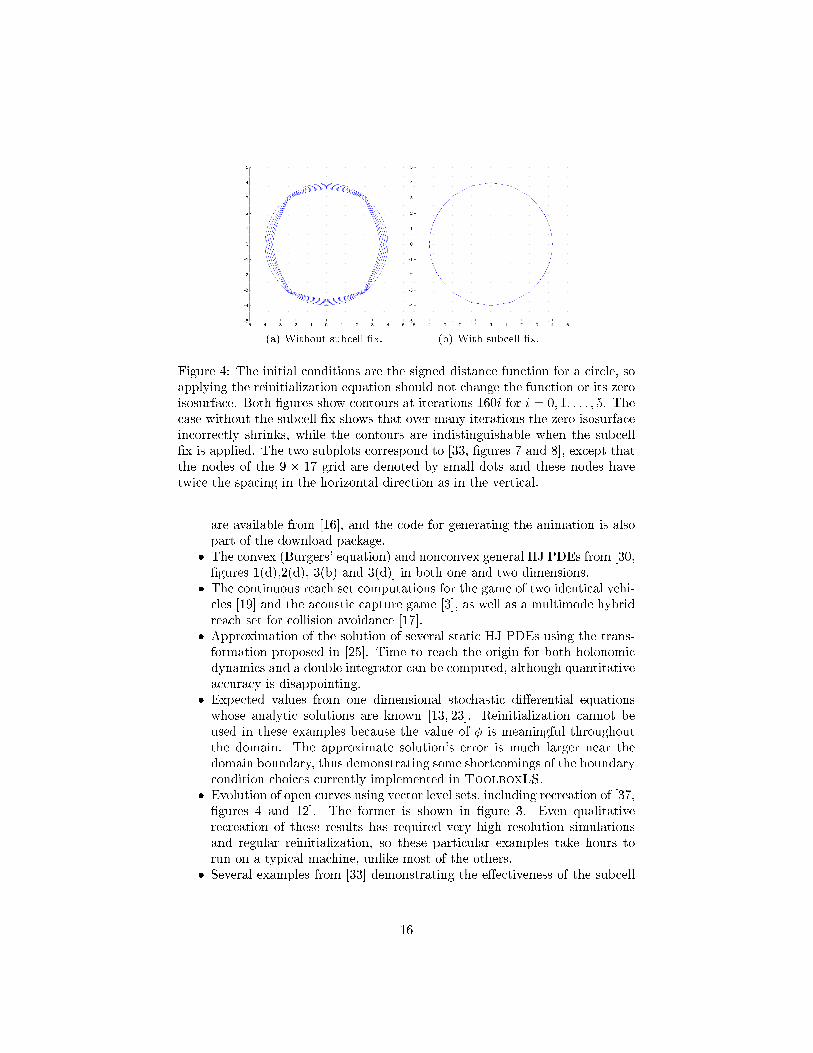
(a) Without subcell �x. (b) With subcell �x.Figure 4: The initial conditions are the signed distance function for a circle, soapplying the reinitialization equation should not change the function or its zeroisosurface. Both �gures show contours at iterations 160i for i = 0; 1; : : : ; 5. Thecase without the subcell �x shows that over many iterations the zero isosurfaceincorrectly shrinks, while the contours are indistinguishable when the subcell�x is applied. The two subplots correspond to [33, �gures 7 and 8], except thatthe nodes of the 9 � 17 grid are denoted by small dots and these nodes havetwice the spacing in the horizontal direction as in the vertical.

are available from [16], and the code for generating the animation is alsopart of the download package.� The convex (Burgers' equation) and nonconvex general HJ PDEs from [30,�gures 1(d),2(d), 3(b) and 3(d)] in both one and two dimensions.� The continuous reach set computations for the game of two identical vehi-cles [19] and the acoustic capture game [3], as well as a multimode hybridreach set for collision avoidance [17].� Approximation of the solution of several static HJ PDEs using the trans-formation proposed in [25]. Time to reach the origin for both holonomicdynamics and a double integrator can be computed, although quantitativeaccuracy is disappointing.� Expected values from one dimensional stochastic di�erential equationswhose analytic solutions are known [13, 23]. Reinitialization cannot beused in these examples because the value of � is meaningful throughoutthe domain. The approximate solution's error is much larger near thedomain boundary, thus demonstrating some shortcomings of the boundarycondition choices currently implemented in ToolboxLS.� Evolution of open curves using vector level sets, including recreation of [37,�gures 4 and 12]. The former is shown in �gure 3. Even qualitativerecreation of these results has required very high resolution simulationsand regular reinitialization, so these particular examples take hours torun on a typical machine, unlike most of the others.� Several examples from [33] demonstrating the e�ectiveness of the subcell16

�x proposed there for maintaining the location of the interface while ap-plying the reinitialization equation. Figure 4 shows how e�ectively thesubcell �x maintains the location of the interface over many iterations.Separate downloads available from [16] include code for computing the expectedtransmission rate and standard deviation of a stochastic hybrid system model ofthe Transmission Control Protocol for transmitting packets on the Internet [20]and an example of optimal control under state constraints [14].While the examples in the Toolbox are primarily aimed at those new to levelset methods, the combination of these examples and the description of internalcoding patterns in section 2.4 should be su�cient for level set researchers toeasily build and test new numerical schemes while leveraging the infrastructureprovided by the Toolbox.

3 Adding New FeaturesIn order to demonstrate the ease with which new schemes are added to Tool-boxLS, we implement an entire class of SSP RK schemes and a monotonemotion by mean curvature approximation. Not only are the implementationsrelatively straightforward, but once they are completed we can easily run a vari-ety of examples to compare the new schemes against existing ones. This abilityto rapidly compare against and build on existing work is one of the primarybene�ts that the Toolbox provides to designers of level set methods.All of the code for the schemes and examples in this section is available asa separate download from [16]; the download also contains some additionalexamples which could not be included in this paper for reasons of length. Testswere performed on a 1.7 GHz Pentium M laptop (from 2004) with 1 GB memoryrunning Windows XP version 2002 with Service Pack 2.3.1 New Temporal Integration SchemesThe explicit SSP RK schemes in [36] were originally directed at approximatingthe solution of conservation laws, but have since been extensively applied to HJPDEs by the level set community. Let p denote the order of the scheme and sthe number of stages. Although schemes with up to p = 5 are given in [36], therestriction to p = s permits only schemes with p � 3 to be implemented withoutproviding a special backward temporal operator; furthermore, the largest CFLcoe�cient that maintains SSP status for the p � 3 schemes is one.A new class of SSP schemes was proposed for conservation laws in [38] withs > p. Relaxing the connection between s and p permits construction of a p = 4

17

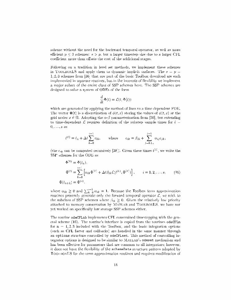
scheme without the need for the backward temporal operator, as well as moree�cient p � 3 schemes: s > p, but a larger timestep size due to a larger CFLcoe�cient more than o�sets the cost of the additional stages.Following on a tradition in level set methods, we implement these schemesin ToolboxLS and apply them to dynamic implicit surfaces. The s = p =1; 2; 3 schemes from [36] that are part of the basic Toolbox download are eachimplemented in separate routines, but in the interests of exiblity we implementa major subset of the entire class of SSP schemes here. The SSP schemes aredesigned to solve a system of ODEs of the form

ddt�(t) = L(t;�(t))which are generated by applying the method of lines to a time-dependent PDE.The vector �(t) is a discretization of �(t; x) storing the values of �(t; x) at thegrid nodes x 2 . Adopting the �-� parameterization from [36], but extendingto time-dependent L requires de�nition of the substep sample times for i =0; : : : ; s as

t(i) = tn +�t i�1Xk=0 cik; where cik = �ik + i�1Xj=k+1�ijcjk;

(the cik can be computed recursively [38]). Given these times t(i), we write theSSP schemes for the ODE as�(0) = �(tn);�(i) = i�1X

k=0h�ik�(k) +�t�ikL(t(k);�(k))i ; i = 1; 2; : : : ; s;

�(tn+1) = �(s):(16)

where �ik � 0 and Pi�1k=0 �ik = 1. Because the Toolbox term approximationroutines presently generate only the forward temporal operator L, we stick tothe subclass of SSP schemes where �ik � 0. Given the relatively low priorityattached to memory conservation by Matlab and ToolboxLS, we have notyet worked on speci�cally low storage SSP schemes either.The routine odeCFLab implements CFL constrained timestepping with the gen-eral scheme (16). The routine's interface is copied from the routines odeCFLnfor n = 1; 2; 3 included with the Toolbox, and the basic integration options(such as CFL factor and callbacks) are handled in the same manner throughan options structure controlled by odeCFLset. This method of controlling in-tegrator options is designed to be similar to Matlab's odeset mechanism andhas been e�ective for parameters that are common to all integrators; however,it does not have the exibility of the schemeData structure pattern adopted byToolboxLS for the term approximation routines and requires modi�cation of

18

Figure 5: The rectangle spins by convection with a velocity �eld that is counter-clockwise rotational motion around the origin. The rectangle also moves out-ward in its normal direction at unit speed for t 2 [0; 1] and inward in its normaldirection at twice that speed for t 2 [1; 1:5]. This particular run used the (2,2)scheme from [36] on a 1012 grid.odeCFLset whenever an integrator with new parameters is introduced.3 As anexperiment, the �-� parameters for the SSP scheme are provided to odeCFLabthrough a structure integratorData added to the end of the parameter list.Although odeCFLab can be directly called by the user to test new schemes, forthe schemes in [36, 38] it is easier to call it indirectly through odeCFLsp, whichchooses the appropriate �-� values from a collection of tables and then callsodeCFLab to do the work. The user must appropriately set the CFL factor totake advantage of the larger timesteps permitted by the s > p schemes.To test the accuracy and e�ciency of these schemes, �ve simple examples wererun. The �rst three involved a three-quarter rotation about the origin underconvective ow of three di�erent initial conditions: (1) a circle centered at theorigin, (2) a rectangle centered at the origin, (3) a pair of slotted disks o�setfrom the origin (a vertically symmetric version of Zalesak's disk [42]). The e�ectof this ow should be rigid body rotation of the initial conditions. The last twoexamples use the circle and rectangle as initial conditions, but in addition to therotational convection the front moves outward at unit speed for the �rst two-thirds of the simulation, and then inward at twice that rate for the �nal third ofthe simulation. This combined motion with the rectangular initial conditions is3A problem that Matlab's odeset shares: consider all of the properties related to Jaco-bians, mass matrices and backward/numerical di�erentiation formulas that odeset containsbut which are entirely ignored by the most commonly used routines ode23 and ode45.

19

shown in �gure 5. The end result of the combined motion should be the sameas that produced by the purely rotational ow|a fact which would not be truefor Zalesak's disk, which is why that initial condition was not used for this ow�eld.The goal of these simulations was to study the e�ect of the order of accuracyof the time integrator on the error in the �nal solution. Unfortunately, errordue to the spatial approximation will inevitably e�ect the outcome. In order tominimize its e�ect, we use a spatial approximation with higher order of accuracythan any of the temporal integrators that we are testing, chose very simple initialconditions, and simulate ow �elds under which the spatial complexity of thefront will not increase.The spatial approximation scheme should achieve its full degree of accuracy forthe circular initial conditions because there are no kinks (derivative disconti-nuities) in the implicit surface function near the interface; however, the lack ofcorners in the interface make this example too simple to be representative oftypical level set problems. The interface in Zalesak's disk has both convex andconcave corners, but we cannot run the second ow �eld for this initial condi-tion. Consequently, we report the results for the rectangular initial conditionshere.The exact implicit surface function for the �nal condition is known: in everycase it is just the initial implicit surface function rotated three-quarters of aturn. To test convergence and order of accuracy, the error at a node is de�nedas the di�erence between the computational solution and the analytic solutionat the �nal time. In the case of the rectangular initial conditions, only the errorsat the nodes within �1=4 �x of the �nal rectangle are included; in other words,a band of width one of nodes lying closest to the rectangle. For the other twoinitial conditions, only the errors at the nodes within �3=2 �x of the interfaceare included.Code for the Toolbox's convection example was modi�ed to construct the appro-priate initial conditions and term approximations, call odeCFLsp, and computethe error. A wrapper routine was then written to execute each of the (s; p)integrators on a sequence of grids for each example.The spatial derivative approximation in all cases was the �fth order accurateWENO approximation from [11]. No reinitialization was performed, and linearlyextrapolated boundary conditions were used at the edge of the computationaldomain. All runs were performed with a CFL coe�cient of 75% of the theoreticalmaximum for stability. Additional details can be found by examining the codein the download package. We specify the integration schemes by the pair (s; p).The schemes tested were the (2; 2) and (3; 3) schemes from [36] and the (3; 2),(4; 2), (4; 3), (5; 3), and (5; 4) schemes from [38]. As expected, the (1; 1) scheme(Forward Euler) was unstable with WENO5, so it was not tested.

20

Figure 6: Convergence plots for the dynamic implicit surface representationof a rectangle integrated by a variety of explicit SSP RK schemes. A �fthorder accurate WENO scheme was used in all cases for the spatial derivatives.The line style legend in the upper right plot applies to all plots. Top row:Purely convective motion. Bottom row: Convection plus motion in the normaldirection (\combination") as shown in �gure 5. Left column: Average error.Right column: Maximum error. Error is measured only at nodes closest tothe analytic solution's interface, and the error is the magnitude of the di�erencebetween the computational and analytic solution at these nodes. For comparisonpurposes, the dotted line in each plot is the grid spacing �x.A few representative results are shown in �gure 6. As can be seen in the �rstrow, the errors for all of the schemes were essentially identical for the purelyconvective case and the rectangular shape. As expected, the convergence rate isfar below that predicted by the formal order of accuracy for the schemes becausethe level set function is not su�ciently smooth. The second row is slightly moreinteresting, as the third and fourth order accurate schemes do show a slightadvantage over the second order accurate schemes, although all of the schemesstill fail to achieve their formal order of accuracy. The maximum error for thiscombination of motion is essentially the same for all schemes. It should be notedthat this combination motion for the rectangle is actually easier than the purely

21

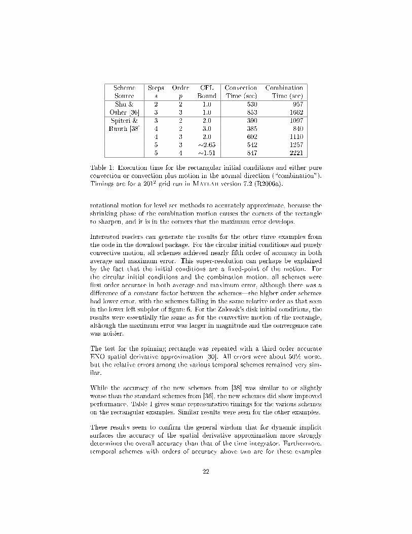
Scheme Steps Order CFL Convection CombinationSource s p Bound Time (sec) Time (sec)Shu & 2 2 1.0 530 957Osher [36] 3 3 1.0 853 1662Spiteri & 3 2 2.0 390 1097Ruuth [38] 4 2 3.0 385 8404 3 2.0 602 11105 3 �2.65 542 12575 4 �1.51 847 2221Table 1: Execution time for the rectangular initial conditions and either pureconvection or convection plus motion in the normal direction (\combination").Timings are for a 2012 grid run in Matlab version 7.2 (R2006a).rotational motion for level set methods to accurately approximate, because theshrinking phase of the combination motion causes the corners of the rectangleto sharpen, and it is in the corners that the maximum error develops.Interested readers can generate the results for the other three examples fromthe code in the download package. For the circular initial conditions and purelyconvective motion, all schemes achieved nearly �fth order of accuracy in bothaverage and maximum error. This super-resolution can perhaps be explainedby the fact that the initial conditions are a �xed-point of the motion. Forthe circular initial conditions and the combination motion, all schemes were�rst order accurate in both average and maximum error, although there was adi�erence of a constant factor between the schemes|the higher order schemeshad lower error, with the schemes falling in the same relative order as that seenin the lower left subplot of �gure 6. For the Zalesak's disk initial conditions, theresults were essentially the same as for the convective motion of the rectangle,although the maximum error was larger in magnitude and the convergence ratewas noisier.The test for the spinning rectangle was repeated with a third order accurateENO spatial derivative approximation [30]. All errors were about 50% worse,but the relative errors among the various temporal schemes remained very sim-ilar.While the accuracy of the new schemes from [38] was similar to or slightlyworse than the standard schemes from [36], the new schemes did show improvedperformance. Table 1 gives some representative timings for the various schemeson the rectangular examples. Similar results were seen for the other examples.These results seem to con�rm the general wisdom that for dynamic implicitsurfaces the accuracy of the spatial derivative approximation more stronglydetermines the overall accuracy than that of the time integrator. Furthermore,temporal schemes with orders of accuracy above two are for these examples

22

largely a waste of e�ort. The most e�cient scheme was the new (4; 2), althoughthe standard modi�ed Euler (2; 2) scheme was nearly as e�ective and in somecases had slightly lower error.The decision to break odeCFLab's parameter compatibility withMatlab's ODEintegrators is an experiment, and could be reversed when this routine is broughtinto the base Toolbox. When the integrators were originally created, it washoped that compatibility with Matlab's ODE routines would make the transi-tion to PDE solvers easier for users and would allow interoperation. Experiencein the �eld seems to indicate instead that the near but not complete compat-ibility is potentially confusing, does not allow interoperation, and is de�nitelylimiting when adding new schemes. If the experiment with the new parame-ter list for odeCFLab proves successful, the existing Toolbox routines could bemodi�ed to accept it (while still remaining backward compatible).Creation of the routines odeCFLab and odeCFLsp required a few hours of coding,plus another few hours to create the examples and debug.3.2 A Monotone Mean Curvature TermWhile new temporal integrators are useful, the form of (1) gives much more ex-ibility to the spatial operator(s), and hence it is new schemes for these termsthat are more often proposed. To demonstrate addition of a new spatial schemeto ToolboxLS, we implement the monotone scheme for motion by mean cur-vature proposed in [21] and further analyzed in [41].The standard approach to the parabolic term (10) is to use the formula

�1� = kDx�k�(�) = kDx�kdiv� Dx�kDx�k�

= dXi=1

@2�@x2i �1kDx�k2

dXi;j=1

@2�@xi@xj @�@xi @�@xj(17)

and approximate the derivatives with centered di�erences [29]. This methodis implemented in the base Toolbox by routines curvatureSecond (which com-putes a second order accurate centered di�erence approximation of the curvatureand gradient) and termCurvature (which handles the operations in (10) andestimates the CFL timestep bound).In [21] it is argued that this scheme is not monotone, and hence we cannot usethe theory in [2] to prove convergence. The proposed alternative for approxi-mating (17) at a node x̂ 2 begins by gathering a stencil of nodes Sx̂ such thateach xk 2 Sx̂ is roughly the same distance from x̂: kxk � x̂k � dx. This stencilwill be roughly circular, must be symmetric with respect to all coordinates, and

23

will thus have an even number of member nodes. The median value of � on thisstencil is then computed��(x̂) = medianf�(xk) j xk 2 Sx̂g; (18)

and the approximation of (17) is�1�(x̂) = 2(��(x̂)� �(x̂))d2x +O(d2x + d�); (19)

(note that (19) �xes several typos in [21, equation (6)]). The small parameterd� measures the angular distance between the members of Sx̂.For some intuition as to why (19) approximates (17), we consider planar (sod = 2). In this case �1� is just a second derivative of � in the direction tangentto the local isosurface of �. Notice that ��(x̂) from (18) will be the averageof the two middle values of f�(xk) j xk 2 Sx̂g. Let the nodes at which thesevalues occur be x0k and x00k . In regions where � is su�ciently smooth, the threepoints x0k, x̂ and x00k will lie on a line `, and ` will be roughly tangent to theisosurface of � at x̂. Straightforward algebra shows that (19) is a standardcentered di�erence approximation of the second derivative along `. We canthen interpret the two components of the error term in (19) as the error in thestandard centered di�erence approximation of the second derivative in a givendirection (O(d2x)), and the error between the direction of ` and the true tangentdirection of the isosurface (O(d�)).This method is implemented in termCurvatureByMedian and oneLaplacian.The former has the same parameter list and is internally almost identical totermCurvature, since it handles various methods by which the user can supplyb(t; x), estimation of the CFL timestep restriction, and (if necessary) bookkeep-ing related to vector level sets. It calls oneLaplacian to compute (18) and (19).Evaluation of these two formulas is straightforward, although it can be memoryintensive depending on the size of the stencil set Sx̂. Because the Toolbox usesa uniform mesh, the stencil set Sx̂ is the same for all nodes x̂ 2 , so we dropthe subscript from S in the remainder of this presentation. The vast majority ofcode in oneLaplacian is devoted to construction of S and its memoization (per-sistent storage of S between function calls so that it need not be reconstructedat each timestep).The user can control the stencil pattern through a stencil width parameter w (apositive integer). We extend the algorithm in [21] to handle grids with di�erentnode spacing in each dimension. Let �x(i) be the spacing in dimension i, andconsider constructing the stencil for node x̂; this stencil can be moved to anyother node by appropriate o�sets. Then we set

�x = max1�i�d�x(i) and dx = w�x

24

(a) S (1 : 1) (b) S (1 : 2) (c) S (1 : 5) (d) S0 (1 : 5)Figure 7: Stencil sets S for stencil width w = 3 on grids with di�erent nodespacings in the di�erent coordinate directions are shown in the three leftmostsubplots. The stencils are built for the node x̂, denoted by a star in the centerof the stencil. The ratio below each plot is (horizontal �x) : (vertical �x). Forcomparison purposes, the intermediate stencil set S 0 is shown in the rightmostsubplot for the grid ratio 1 : 5. Note that many of the nodes in S 0 lie in similaror identical directions from the center node.and create an initial stencil set

S 0 = �xk 2 j dx � 12�x � kxk � x̂k < dx + 12�x :By including nodes in a band of width �x around the desired stencil radius dx,we ensure that S 0 includes at least nodes along every coordinate axis. However,when the �x(i) are not equal for all i, the nodes in S 0 may show considerable biastoward some directions; for example, there may be multiple nodes in exactly thesame direction (along the coordinate axis) if 2�x(j) < �x for some dimensionj. To reduce this bias, we add node xl 2 S 0 to the �nal stencil set S only if

xl � x̂kxl � x̂k � xk � x̂kxk � x̂k � cos(� ~d�)for all fxk 2 S 0 j jkxk � x̂k � dxj < jkxl � x̂k � dxjg:

In words, a node is added to the �nal stencil set S only if it is in a direction whichmakes an angle of at least � ~d� with all nodes in S 0 which are closer to the desiredstencil width dx, where ~d� is an estimate of the angular accuracy parameter d�and � is some fractional constant (we use � = 1=4). The goal is to choose astencil set S whose angular sampling in every direction is roughly constant.The resulting stencil sets for several two dimensional grids with varying ratiosof �x(1) to �x(2) are shown in �gure 7 for w = 3.Any procedure for constructing S inevitably chooses nodes that are not preciselydistance dx from x̂. As proposed in [41], we can adjust for this inconsistencyusing linear interpolation. Instead of (18), we use the de�nition

��(x̂) = medianf~�(xk) j xk 2 Sx̂g; (20)25

(a) �1(x) (b) Analytic �1�1(x) (c) Median-based approxi-mation of �1�1(x)Figure 8: The test polynomial �1(x), the analytic �1�1(x), and the median-based approximation of �1�1(x) for a stencil with w = 3 on a 1012 grid. Notethat for better visualization the view of �1(x) is rotated 180� in azimuth com-pared to the other two plots. Because S only includes eight distinct directionsfor this w, the median-based approximation displays signi�cant quantization.where we interpolate a value ~�(xk) at a point exactly dx along the line betweenx̂ and xk ~�(xk) = �(x̂) + dxkxk � x̂k (�(xk)� �(x̂)):Such interpolation also makes it possible to use a square stencil for S, instead ofthe approximately circular one discussed above. Although originally proposedin [21] without interpolation, such square stencils are only consistent approxi-mations of �1 when interpolation is used.To study the accuracy of the median-based approximation, we use a polynomialproposed in [21]

�1(x) = 6x1 + 54x2 + 92 x212 + 145 x1x2 + 265 x222 ; (21)

whose analytic curvature can be derived. Results similar to those describedbelow are also observed for the other test polynomial proposed in [21]. Repre-sentative plots of the value of �1(x), the analytic �1�1(x) and the median-basedapproximation for w = 3 are shown in �gure 8. Notice the stair-step nature ofthe median-based approximation|because only a small number of directionsis available in the stencil, there are only a small number of possible values forthe approximation. We do not include a plot of the standard centered di�er-ence approximation of �1�1(x) because it is visually indistinguishable from theanalytic solution.While the error in the median-based scheme (19) is O(d2x + d�), for a grid with�xed connectivity we do not have direct control over d� in the algorithm de-scribed above because we are constrained to use neighboring nodes to construct��(xk). We decrease d� indirectly by increasing the stencil width w. For agrid with �xed �x, increasing w leads to an increase in dx = w�x. It is not

26

Circular Stencil Square StencilRatio Stencil Grid w/o interp w/ interp w/ interp�x Radius Size Mean Max Mean Max Mean Max1 : 1 1 101� 101 1.995 6.523 1.439 5.459 1.439 5.4592 284� 284 1.425 3.704 1.191 3.554 0.896 2.9603 521� 521 0.878 2.652 0.796 2.654 0.708 2.3024 801� 801 0.560 1.647 0.433 1.197 0.604 2.0135 1119� 1119 0.565 1.696 0.493 1.591 0.547 1.8541 : 2 1 101� 51 1.720 6.436 1.094 5.353 1.094 5.3532 284� 142 0.929 3.669 0.670 2.580 0.737 2.7823 521� 261 0.614 2.179 0.445 2.047 0.579 2.2934 801� 401 0.476 1.642 0.347 1.488 0.512 2.0075 1119� 560 0.401 1.216 0.295 1.162 0.477 1.8491 : 5 1 126� 26 1.517 6.271 0.938 5.125 0.888 5.1252 355� 72 0.825 2.739 0.607 2.536 0.601 2.8963 651� 131 0.593 2.137 0.429 1.830 0.503 2.2714 1001� 201 0.482 1.751 0.351 1.464 0.458 1.9965 1399� 281 0.378 1.173 0.271 1.040 0.437 1.843Table 2: Error in the median approximation of �1�1(x) as d� and dx are de-creased at roughly the optimal theoretical rate. The polynomial �1(x) is givenin (21). The error in this median-based scheme is enormous and does not con-sistently achieve its theoretical order of accuracy.discussed in [21, 41] and it is not immediately obvious that we can achieve aconsistent scheme O(d2x + d�) ! 0 through some combination of �x ! 0 andw ! +1. To show that consistency is possible, note that the number of nodesin the stencil jSj has asymptotic behaviour

jSj = O�circumference of stencildistance between xk� = O�2�dx�x

� = O(�x �1);where we have used the ansatz dx = �x for some unknown constant . Sinced� = O(jSj�1), we see that the error in (19) is O(�x2 + �x1� ). Balancingthe exponents leads to the choice = 1=3, asymptotic error O(�x2=3) and con-sistency. Of course, our control over dx is indirect through stencil width w, so tostudy the convergence of the scheme experimentally using the algorithm abovewe choose a sequence of w values and adjust �x according to

w�x = dx = �x = �x1=3 =) �x = w�3=2Using this relationship between w and �x we approximate �1�1(x) on a varietyof grids and record the error in the approximation in table 2. When comparedto a typical error of � 10�10 in the standard centered di�erence approximationsof �1�1 for these grids, the error in the median-based approach is terrible. Fur-thermore, although the error is decreasing as the grid is re�ned, the theoreticalorder of accuracy (�x)2=3 is not always achieved; in fact, the error for w = 5 onthe 1 : 1 grid is actually larger than for w = 4. It should be noted that using

27

interpolation (20) provides a signi�cant bene�t at all stencil sizes when com-pared to computing the median without interpolation (18). The square stencilis cheaper to construct (no need to search for a set of nodes approximating acircle) but is more expensive to evaluate (there are more nodes) and is generallynot as accurate as the circular stencil with interpolation.Given that the quantitative error in the median-based approximation is so large,why use it? The monotonicity of the median-based approximation is a nice fea-ture from a theoretical perspective, but we know of no practical problems wherethe failure of the standard centered di�erence approximation to be monotoneresults in a signi�cant degradation of the approximate solution when comparedwith the results from the median-based scheme.Instead, the reason to use the new scheme is its speed. Motion by mean cur-vature (10) is often used as a regularizing term in applications like image seg-mentation. In these applications it is the qualitative attening of the frontgenerated by �1 that is more important than a speci�c quantitative solution.To examine the qualitative e�ectiveness of the median-based approximation, in�gure 9 we apply a variety of approximations of (10) to a star-shaped initialinterface [27, �gure 4.2]. Despite the poor quantitative accuracy of the median-based approximation, in motion by mean curvature the results are qualitativelyvery similar to the much higher accuracy standard centered di�erence approx-imation. Furthermore, the CFL timestep restriction is O(d2x) = O(w2�x2), sofor large w much longer timesteps can be taken and execution is considerablyfaster. In fact, the implementation in oneLaplacian becomes quite memory in-tensive for large w and hence rather slow; it is likely that a compiled implemen-tation of the median-based scheme would have an even larger speed advantageover the standard centered di�erence scheme.In addition to code for the tests presented here, the download package includescode recreating many of the examples from [21]. Creation of termCurvatureByMedianand oneLaplacian took several days, most of which was devoted to designingthe algorithm to generate and memoize stencils on grids with variable �x. Thecollection of examples and tests took about two days to �ll in, using existing ex-amples as a starting point. While termCurvatureByMedian and oneLaplacianare written to be dimensionally independent, they have not yet been tested indimensions greater than two.

4 Conclusion and Future WorkWe intend for ToolboxLS to be useful to the research community in at leastthree ways. The �rst is to make easy-to-use and reasonably e�cient implementa-tions of high accuracy methods available to application scientists and engineers

28

(a) Standard centered di�erence approximation (132 seconds)

(b) Circular stencil w = 1 with interpolation (619 seconds)

(c) Circular stencil w = 3 with interpolation (78 seconds)

(d) Circular stencil w = 5 with interpolation (35 seconds)

(e) Square stencil w = 3 with interpolation (87 seconds)Figure 9: Motion by mean curvature of a star-shaped front using various approx-imations of �1. The grid is 2012 nodes and the standard (2,2) time integrationscheme is used. The median-based approximation may have poor quanitativeaccuracy, but its qualitative results are very similar to those of the standardcentered �nite di�erence, and for larger stencils it is signi�cantly faster.

29

unfamiliar with the details of level set methods. The second is to furnish a ex-ible environment in which designers of level set methods can experiment withnew schemes. The third is to provide a common software infrastructure thatwill aid in testing, comparison and distribution of those schemes in the spiritof reproducible research. This article has emphasized the latter two goals bypresenting only a brief overview of the current Toolbox contents and devotingsigni�cant space to explaining some common internal design patterns used inthe code that promote both e�ciency and exibility. The implementation oftwo new schemes for the Toolbox was also described, including an experimentalmodi�cation of the time integrator's parameter list based on user feedback.For the level set methods that it implements, ToolboxLS manages reasonablee�ciency by Matlab-style vectorization, which involves sequential access tolarge data arrays. Syntactic tricks involvingMatlab's cell array data type per-mit almost all level set operations to be written in a dimensionally independentmanner. Furthermore, all of ToolboxLS is written in m-�les, so there is nooverhead to installing, executing or examining the code.Additional level set features that we eventually hope to add to ToolboxLSinclude:

� More general and higher order accurate boundary conditions.� Additional spatial derivative approximation schemes (such as third orderaccurate WENO).� ENO/WENO function value interpolation (not just gradients) throughout (not just at nodes).� Evolution of codimension two curves in R3 using vector level sets.� The \Roe with entropy �x" numerical Hamiltonian [30], which may intro-duce less arti�cial dissipation that Lax-Friedrichs.A signi�cant shortcoming of the present Toolbox is the lack of a Fast Marchingstyle algorithm [34] for solving the Eikonal equation kDx�k = 1 and similarstatic HJ PDEs. These equations play a key role in many dynamic implicitsurface applications requiring reinitialization and/or velocity extension [1]. Un-fortunately, these algorithms also have a random data access pattern for whichMatlab m-�le implementations are extremely ine�cient. It is possible to cre-ate compiled implementations that interface through MEX to Matlab. Wehave performed some experiments with such implementation schemes, but theirpotential inclusion into ToolboxLS raises issues with distribution (users wouldhave to compile), debugging (breakpoints cannot easily be set inside MEX rou-tines), exibility (MEX �les are much more di�cult to modify than m-�les),and readability (users would need to know another language). We are open tocomments regarding methods by which these issues might be minimized.In fact, users of ToolboxLS should consider it to be a work in progress, andsuggestions related to interfaces, schemes, implementations and/or applicationsare welcome.

30

Acknowledgements: A project the size of ToolboxLS is not constructed inisolation. The author would like to thank Ronald Fedkiw and Stanley Osherfor extensive discussions about the details of numerical schemes for solving theHamilton-Jacobi PDE. Additional discussions with David Adalsteinsson, KenAlton, Jean-Pierre Aubin, Alexandre Bayen, Doug Enright, L. C. Evans, Chiu-Yen Kao, Alexander Kurzhanski, Doron Levy, John Lygeros, Jianliang Qian,Steven Ruuth, Patrick Saint-Pierre, James Sethian, Pravin Varaiya, AlexanderVladimirsky, Hong-Kai Zhao and many others have contributed to my under-standing of the �eld. The support of Claire Tomlin and Shankar Sastry madepossible two earlier implementations, from which the current design bene�tedimmensely. Development of the new schemes in section 3 was motivated bydiscussions with Adam Oberman and Raymond Spiteri (who pointed out theinstability of Forward Euler and WENO5). The author would also like to thankAdam Oberman and Ken Alton for their comments on a draft of this paper.Development and release of the code and documentation for ToolboxLS is sup-ported by a grant from the National Science and Engineering Research Councilof Canada.

References[1] D. Adalsteinsson and J. A. Sethian, \The fast construction of extension velocitiesin level set methods," Journal of Computational Physics, vol. 148, pp. 2{22, 1999.[2] G. Barles and P. E. Souganidis, \Convergence of approximation schemes for fullynonlinear second order equations," Asymptotic Analysis, vol. 4, no. 3, pp. 271{283, 1991.[3] P. Cardaliaguet, M. Quincampoix, and P. Saint-Pierre, \Set-valued numericalanalysis for optimal control and di�erential games," in Stochastic and Di�erential

Games: Theory and Numerical Methods, ser. Annals of International Societyof Dynamic Games, M. Bardi, T. E. S. Raghavan, and T. Parthasarathy, Eds.Birkh�auser, 1999, vol. 4, pp. 177{247.[4] D. Chopp, \Computing minimal surfaces via level set curvature ow," Journal ofComputational Physics, vol. 106, pp. 77{91, 1993.[5] K. T. Chu and M. Prodanovic, \Level set method library (LSMLIB)." [Online].Available: http://www.princeton.edu/�ktchu/software/lsmlib/[6] M. G. Crandall and P.-L. Lions, \Viscosity solutions of Hamilton-Jacobi equa-tions," Transactions of the American Mathematical Society, vol. 277, no. 1, pp.1{42, 1983.[7] ||, \Two approximations of solutions of Hamilton-Jacobi equations," Mathe-matics of Computation, vol. 43, no. 167, pp. 1{19, 1984.[8] M. G. Crandall, H. Ishii, and P.-L. Lions, \User's guide to viscosity solutions ofsecond order partial di�erential equations," Bulletin of the American Mathemat-ical Society, vol. 27, no. 1, pp. 1{67, 1992.[9] [Online]. Available: http://creativecommons.org

31

[10] R. Fedkiw, T. Aslam, B. Merriman, and S. Osher, \A non-oscillatory Eulerianapproach to interfaces in multimaterial ows (the ghost uid method)," Journalof Computational Physics, vol. 152, pp. 457{492, 1999.[11] G.-S. Jiang and D. Peng, \Weighted ENO schemes for Hamilton-Jacobi equa-tions," SIAM J. Sci. Comput., vol. 21, pp. 2126{2143, 2000.[12] C.-Y. Kao, S. Osher, and J. Qian, \Lax-Friedrichs sweeping schemes for staticHamilton-Jacobi equations," Journal of Computational Physics, vol. 196, pp. 367{391, 2004.[13] P. E. Kloeden and E. Platen, Numerical Solution of Stochastic Di�erential Equa-tions, 3rd ed., ser. Applications of Mathematics. Springer, 1999.[14] A. B. Kurzhanski, I. M. Mitchell, and P. Varaiya, \Control synthesis for state con-strained systems and obstacle problems," in Proceedings of the IFAC Workshopon Nonlinear Control (NOLCOS), Vienna, Austria, 2004.[15] V. Mallet, \Multivac C++ library." [Online]. Available: http://vivienmallet.net/fronts/index.php[16] [Online]. Available: http://www.cs.ubc.ca/�mitchell/ToolboxLS[17] I. Mitchell and C. Tomlin, \Level set methods for computation in hybrid systems,"in Hybrid Systems: Computation and Control, ser. Lecture Notes in ComputerScience, B. Krogh and N. Lynch, Eds. Springer Verlag, 2000, no. 1790, pp.310{323.[18] I. M. Mitchell, \A toolbox of level set methods (version 1.1)," Departmentof Computer Science, University of British Columbia, Vancouver, BC,Canada, Tech. Rep. TR-2007-11, June 2007. [Online]. Available: http://www.cs.ubc.ca/�mitchell/ToolboxLS/toolboxLS.pdf[19] I. M. Mitchell, A. M. Bayen, and C. J. Tomlin, \A time-dependent Hamilton-Jacobi formulation of reachable sets for continuous dynamic games," IEEE Trans-actions on Automatic Control, vol. 50, no. 7, pp. 947{957, 2005.[20] I. M. Mitchell and J. A. Templeton, \A toolbox of Hamilton-Jacobi solvers foranalysis of nondeterministic continuous and hybrid systems," in Hybrid Systems:Computation and Control, ser. Lecture Notes in Computer Science, M. Morariand L. Thiele, Eds. Springer Verlag, 2005, no. 3414, pp. 480{494.[21] A. Oberman, \A convergent upwind di�erence scheme for motion of level sets bymean curvature," Numerische Mathematik, vol. 99, no. 2, pp. 365{379, 2004.[22] ||, \Convergent di�erence schemes for degenerate elliptic and parabolic equa-tions: Hamilton-Jacobi equations and free boundary problems," SIAM Journalon Numerical Analysis, vol. 44, no. 2, pp. 879{895, 2006.[23] B. �ksendal, Stochastic Di�erential Equations: an Introduction with Applications,6th ed. Springer, 2003.[24] Journal of Scienti�c Computing, vol. 19, no. 1{3, 2003.[25] S. Osher, \A level set formulation for the solution of the Dirichlet problem forHamilton-Jacobi equations," SIAM Journal of Mathematical Analysis, vol. 24,no. 5, pp. 1145{1152, 1993.[26] S. Osher and R. Fedkiw, \Level set methods: An overview and some recentresults," Journal of Computational Physics, vol. 169, pp. 463{502, 2001.

32

[27] ||, Level Set Methods and Dynamic Implicit Surfaces. Springer, 2002.[28] S. Osher and N. Paragios, Eds., Geometric Level Set Methods in Imaging, Visionand Graphics. Springer, 2003.[29] S. Osher and J. A. Sethian, \Fronts propagating with curvature-dependent speed:Algorithms based on Hamilton-Jacobi formulations," Journal of ComputationalPhysics, vol. 79, no. 1, pp. 12{49, 1988.[30] S. Osher and C.-W. Shu, \High-order essentially nonoscillatory schemes forHamilton-Jacobi equations," SIAM Journal on Numerical Analysis, vol. 28, no. 4,pp. 907{922, 1991.[31] D. Peng, B. Merriman, S. Osher, H. Zhao, and M. Kang, \A PDE based fastlocal level set method," Journal of Computational Physics, vol. 165, pp. 410{438,1999.[32] G. Peyr�e, \Toolbox fast marching." [Online]. Available: http://www.mathworks.com/matlabcentral/�leexchange/loadFile.do?objectId=6110[33] G. Russo and P. Smereka, \A remark on computing distance functions," Journalof Computational Physics, vol. 163, pp. 51{67, 2000.[34] J. A. Sethian, Level Set Methods and Fast Marching Methods. New York: Cam-bridge University Press, 1999.[35] ||, \Evolution, implementation, and application of level set and fast marchingmethods for advancing fronts," Journal of Computational Physics, vol. 169, pp.503{555, 2001.[36] C.-W. Shu and S. Osher, \E�cient implementation of essentially non-oscillatoryshock-capturing schemes," Journal of Computational Physics, vol. 77, pp. 439{471, 1988.[37] P. Smereka, \Spiral crystal growth," Physica D, vol. 138, pp. 282{301, 2000.[38] R. J. Spiteri and S. J. Ruuth, \A new class of optimal high-order strong-stability-preserving time discretization methods," SIAM Journal on Numerical Analysis,vol. 40, no. 2, pp. 469{491, 2002.[39] B. Sumengen, \A Matlab toolbox implementing level set methods." [Online].Available: http://barissumengen.com/level set methods/index.html[40] M. Sussman, P. Smereka, and S. Osher, \An improved level set method for in-compressible two-phase ow," Journal of Computational Physics, vol. 114, pp.145{159, 1994.[41] R. Takei, \Modern theory of numerical methods for motion by mean curvature,"Master's thesis, Department of Mathematics, Simon Fraser University, August2007.[42] S. T. Zalesak, \Fully multidimensional ux-corrected transport algorithms for uids," Journal of Computational Physics, vol. 31, no. 3, pp. 335{362, June 1979.

33