The Fluctuation Theoremand Green-Kubo Relations

Debra J. Searles* and Denis J. Evans#

*Department of Chemistry, University of Queensland,

Brisbane, QLD 4072, Australia

#Research School of Chemistry, Australian National University, GPO Box 414,

Canberra, ACT 2601, Australia

Abstract

Green-Kubo and Einstein expressions for the transport coefficients of a fluid in a

nonequilibrium steady state can be derived using the Fluctuation Theorem and by assuming

the probability distribution of the time-averaged dissipative flux is Gaussian. These

expressions are consistent with those obtained using linear response theory and are valid in

the linear regime. It is shown that these expressions are however, not valid in the nonlinear

regime where the fluid is driven far from equilibrium. We advance an argument for why

these expressions are only valid in the linear response, zero field limit.

I. INTRODUCTION

In 1993 Evans, Cohen and Morriss [1], ECM2, gave a quite general formula for the

logarithm of the probability ratio that in a nonequilibrium steady state, the time averaged

dissipative flux takes on a value, J t+ ( ), to minus that value, namely, J t J t− += −( ) ( ) . That is

they gave a formula for ln[ ( ( )) / ( ( ))]p J t p J t+ − from a natural invariant measure [1, 2]. This

formula gives an analytic expression for the probability that, for a finite system and for a

finite time, the dissipative flux flows in the reverse direction to that required by the Second

Law of Thermodynamics. The formula has come to be known as the Fluctuation Theorem,

FT. Surprisingly perhaps, it is valid far from equilibrium in the nonlinear response regime

[1]. Since 1993 there have been a number of derivations and generalisations of the FT.

Evans and Searles [3-5] gave a derivation, similar to that given here, which considered

transient, rather than steady state, nonequilibrium averages and employed the Liouville

measure. Gallavotti and Cohen [6,7], gave a proof of the formula for a nonequilibrium

stationary state, based on a Chaotic Hypothesis and employing the SRB measure. In the long

time limit, when steady state averages are independent of the initial phase used to generate the

steady state trajectory, averages over transient segments which originate from the initial

equilibrium microcanonical ensemble can be expected to approach those taken over

nonequilibrium steady state segments. Thus for chaotic systems both approaches should be

able to explain the steady state results. However this point is being debated [8]. Other

generalisations of the FT have recently been developed [9-12].

In a footnote to their original paper ECM2 also pointed out that in the weak field regime,

there was a connection between the FT, the Central Limit Theorem (CLT) [13, 14], and

Green-Kubo relations [1, 4]. In the present paper we explore this connection further and

consider the validity of the Green-Kubo relations far from equilibrium. We show that if the

distribution of the time averaged dissipative flux, p J t( ( )), is Gaussian arbitrarily far from the

mean, then from the FT one can derive both generalised Einstein and generalised Green-Kubo

relations for the relevant transport coefficient. Both isothermal (ie isokinetic) and

isoenergetic dynamics are considered. We conduct computer simulations which prove that

outside the linear regime, these generalised Green-Kubo and Einstein relations are incorrect.

2

It turns out, that in order for the nonlinear Green-Kubo relations to be valid p J tJ t

( ( ) )( )

σ must

be a normalised Gaussian when both t and J tJ t

( )( )

σ → ∞ . However, this is not guaranteed

by the Central Limit theorem [15] and the nonlinear Green-Kubo relations are invalid.

3

II. NEMD DYNAMICAL SYSTEMS

The development of NonEquilibrium Molecular Dynamics, NEMD, over the previous two

decades has lead to a set of deterministic algorithms (ie N-particle dynamical systems) from

which one can in principle, calculate correct values for each of the Navier-Stokes transport

coefficients [16]. These dynamical systems actually duplicate the salient features of real

experimental nonequilibrium steady states. In the linear regime close to equilibrium,

nonequilibrium statistical mechanics is used to prove that in the large system limit the

calculated transport properties are correct. Using NEMD one can calculate far more than just

transport coefficients. One can also correctly calculate the changes to the local molecular

structure and dynamics, caused by the applied external fields.

Consider an N-particle system in 3 Cartesian dimensions, with coordinates and peculiar

momenta, { , ,.. , ,.. } ( , )q q q p p q p1 2 1N N ≡ ≡ ΓΓ. The internal energy of the system is

H p mii

N

02

1

2≡ +=∑ / ( )Φ q where Φ(q) is the interparticle potential energy which is a function

of the coordinates of all of the particles, q. In the presence of an external field Fe, the

thermostatted equations of motion are taken to be,

˙ / ( )q p Ci i i em F= + ΓΓ

˙ ( ) ( ) ( )p F q D pi i i e iF= + −ΓΓ ΓΓα (1)

where

F q q qi i( ) ( ) /= − ∂∂Φ (2)

and α is the thermostat multiplier derived from Gauss’ Principle of Least Constraint in order

to fix the peculiar kinetic energy, K p mii

N

≡=∑ 2

1

2/ , or the internal energy, H0. In a constant

energy system the thermostat multiplier is easily seen to be,

αE eJ VF K= − ( ) /ΓΓ 2 (3)

while in an isokinetic system the corresponding expression for the multiplier is,

4

αK

ii i em

F

K=• +∑ p

F D( )

2 . (4)

We note that the thermostatted equations of motion are time reversible. The dissipative flux

is defined in terms of the adiabatic (ie unthermostatted) derivative of the internal energy,

˙ ( )H J VFade0 ≡ − ΓΓ (5)

where V is the system volume.

In an isokinetic system, the balance between the work done on the system by the external

field and the heat removed by the thermostat implies that

lim ( ( )) lim ( ( ))( ) ( )t

t

et

t

Kds J s VF K ds s→∞ →∞∫ ∫= −

00

0

2ΓΓ ΓΓα , (6)

while in a constant energy system, energy balance is exact instantaneously,

J VF Ke E( ) ( ) ( )ΓΓ ΓΓ= −2 p α . (7)

In equation (6), K0 is the (fixed) peculiar kinetic energy,

3NkBT / 2 ≡ 3Nβ0−1 / 2 ≡ K0 . (8)

A shorthand notation will be used to refer to the time averaged value of a phase function

along a trajectory segment, ΓΓ+ < <( );s s t0 . We will write,

A t t ds A st

+ +≡ ∫( ) ( ( ))1

0

ΓΓ . (9)

Since the dynamics is time reversible, for every trajectory segment ΓΓ+ < <( );s s t0 , there

exists an antisegment, ΓΓ− < <( );s s t0 . A plus or minus sign is ascribed to a particular

trajectory segment depending on the sign of the time averaged value of the thermostat

multiplier: therefore by definition α+ >( )t 0. The time reversed conjugate of the segment

ΓΓ+ < <( );s s t0 , namely ΓΓ− < <( );s s t0 , is termed an antisegment and,

5

A t t ds A st

− −≡ ∫( ) ( ( ))1

0

ΓΓ . (10)

Depending on the parity of the phase function A( )ΓΓ under the time reversal mapping there

may be a simple relation between A t+ ( ) and A t− ( ) . Without loss of generality we take the

external field to be even under time reversal symmetry, therefore the dissipative flux is odd

and,

J t J t t− += − ∀( ) ( ), . (11)

Using this notation the dissipative flux is related to the phase space compression

accomplished by the thermostat,

lim(t→ ∞)

βJ+(t)VFe = − lim(t→ ∞)

3Nα +(t) isokinetic

βJ+(t)VFe = −3Nα +(t) isoenergetic

(12)

where for both the isokinetic and isoenergetic systems,

βJ(G )V ≡ 3NJ(G )V / 2K(p )

but in the isokinetic case, the peculiar kinetic energy K is a constant of the motion. Since β is

always positive, we see from (12), that the sign convention for distinguishing segments and

antisegments can equally well be taken from the sign of the dissipative flux.

6

III. THE (TRANSIENT) FLUCTUATION THEOREM

For our system, since the adiabatic incompressibility of phase space (AIG) holds [16], the

Liouville equation for the N-particle distribution function f t( , )ΓΓ , reads,

df tdt

f t N f t O f t( , )

( , ) ˙ ( ) ( , ) ( ) ( , )ΓΓ ΓΓ ΓΓ

ΓΓ ΓΓ ΓΓ ΓΓ= − • = +∂∂ α3 1 . (13)

The O(1) terms are omitted in the following discussion. Incorporation of these terms poses

no difficulty but complicates the expressions and the consequences can be neglected in the

large system limit. The solution of this equation can be written as [4]

f t t N s ds f

N t t f

t

( ( ), ) exp[ ( ( )) ] ( , )

exp[ ( ) ] ( , )

ΓΓ ΓΓ ΓΓ

ΓΓ

± ± ±

± ±

=

=

∫3 0

3 0

0

α

α. (14)

This is known as the Lagrangian form of the Kawasaki distribution function [4].

Consider the propagation of a phase point along a trajectory in phase space. If we select

an initial, t = 0, phase, G(1), and we advance time from 0 to τ using the equations of motion (1)

we obtain G(2) = G(τ;G(1)) = exp[iL(G(1),Fe)τ]G(1), where the phase Liouvillean, iL(G(1),Fe), is

defined as, iL F F Fe e e( , ) ˙ ( , ) ˙ ( , )ΓΓ ΓΓ ΓΓ≡ • ∂ ∂ + • ∂ ∂q q p p. Continuing on to 2τ gives G(3) =

exp[iL(G(2),Fe)τ]G(2) = exp[iL(G(1),Fe)2τ]G(1). This is demonstrated in Figure 1.

From this trajectory segment, we can construct a time-reversed trajectory. At the midpoint

of the trajectory segment G(1,3) (i.e. at t = τ) we apply the time reversal mapping, M(T), to G(2)

generating M(T)G(2) ≡ G(5). If we now propagate backward in time keeping the same external

field, we obtain G(4) = exp[-iL(G(5),Fe)τ]G (5). G(4) is the initial t = 0 phase from which a

segment G(4,6) can be generated with G(6) = exp[iL(G(4),Fe)2τ]G(4). We denote the trajectory τ-

segment G(1)→G (3), as ΓΓ ΓΓ( , )1 3 = + ; similarly ΓΓ ΓΓ( , )4 6 = − . Using the symmetry of the

equations of motion it is trivial to show that, J(G(2)) = −J(G(5)) and that J(t; ΓΓ+ , 0 < t < 2τ) =

−J(2τ-t; ΓΓ− , 0 < t <2τ), - see Figure 1. We now have an algorithm for finding initial phases

7

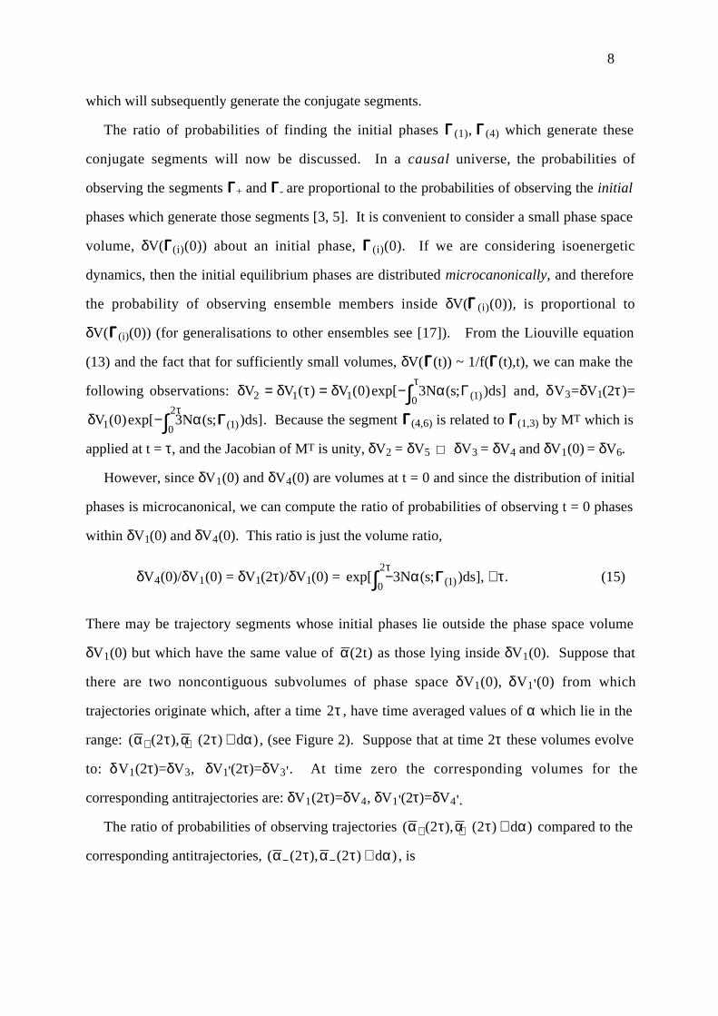
which will subsequently generate the conjugate segments.

The ratio of probabilities of finding the initial phases G(1), G(4) which generate these

conjugate segments will now be discussed. In a causal universe, the probabilities of

observing the segments G+ and G- are proportional to the probabilities of observing the initial

phases which generate those segments [3, 5]. It is convenient to consider a small phase space

volume, δV(G(i)(0)) about an initial phase, G (i)(0). If we are considering isoenergetic

dynamics, then the initial equilibrium phases are distributed microcanonically, and therefore

the probability of observing ensemble members inside δV(G (i)(0)), is proportional to

δV(G(i)(0)) (for generalisations to other ensembles see [17]). From the Liouville equation

(13) and the fact that for sufficiently small volumes, δV(G(t)) ~ 1/f(G(t),t), we can make the

following observations: δ δ τ δ ατ

V V V N s ds2 1 1 100 3= = −∫( ) ( )exp[ ( ; ) ]( )Γ and, δV3=δV1(2τ)=

δ ατ

V N s ds1 10

20 3( )exp[ ( ; ) ]( )−∫ ΓΓ . Because the segment G(4,6) is related to G(1,3) by MT which is

applied at t = τ, and the Jacobian of MT is unity, δV2 = δV5 ⇒ δV3 = δV4 and δV1(0) = δV6.

However, since δV1(0) and δV4(0) are volumes at t = 0 and since the distribution of initial

phases is microcanonical, we can compute the ratio of probabilities of observing t = 0 phases

within δV1(0) and δV4(0). This ratio is just the volume ratio,

δV4(0)/δV1(0) = δV1(2τ)/δV1(0) = exp[ ( ; ) ]( )−∫ 3 10

2N s dsα

τΓΓ , ∀τ. (15)

There may be trajectory segments whose initial phases lie outside the phase space volume

δV1(0) but which have the same value of α( )2t as those lying inside δV1(0). Suppose that

there are two noncontiguous subvolumes of phase space δV1(0), δV1'(0) from which

trajectories originate which, after a time 2τ , have time averaged values of α which lie in the

range: ( ( ), ( ) )α τ α τ α+ + +2 2 d , (see Figure 2). Suppose that at time 2τ these volumes evolve

to: δV1(2τ)=δV3, δV1'(2τ)=δV3'. At time zero the corresponding volumes for the

corresponding antitrajectories are: δV1(2τ)=δV4, δV1'(2τ)=δV4'.

The ratio of probabilities of observing trajectories ( ( ), ( ) )α τ α τ α+ + +2 2 d compared to the

corresponding antitrajectories, ( ( ), ( ) )α τ α τ α− − +2 2 d , is

8

( )( )

( )( )

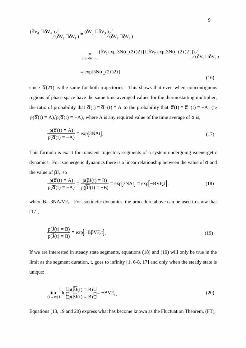
( exp[ ( ) ] exp[ ( ) ])( )

exp[ ( ) ]

''

''

lim'

'

δ δδ δ

δ δδ δ

δ α τ τ δ α τ τδ δ

α τ τ

α

V VV V

V VV V

V N V NV V

N

4 41 1

3 31 1

1 11 1

3 2 2 3 2 2

3 2 2

++ = +

+

= ++

=

→+ +

+

d 0

(16)

since α τ( )2 is the same for both trajectories. This shows that even when noncontiguous

regions of phase space have the same time averaged values for the thermostatting multiplier,

the ratio of probability that α α( ) ( )t t A= =+ to the probability that α α( ) ( )t t A= = −− , (ie

p t A p t A( ( ) ) ( ( ) )α α= = − , where A is any required value of the time average of α is,

p t A

p t ANAt

( ( ) )

( ( ) )exp

αα

== −

= [ ]3 . (17)

This formula is exact for transient trajectory segments of a system undergoing isoenergetic

dynamics. For isoenergetic dynamics there is a linear relationship between the value of α and

the value of βJ, so

p t A

p t A

p J t B

p J t BNAt BVF te

( ( ) )

( ( ) )

( ( ) )

( ( ) )exp exp

αα

ββ

== −

= == −

= [ ] = −[ ]3 . (18)

where B=-3NA/VFe. For isokinetic dynamics, the procedure above can be used to show that

[17],

p J t B

p J t BB VF te

( ( ) )

( ( ) )exp

==

= −[ ]β . (19)

If we are interested in steady state segments, equations (18) and (19) will only be true in the

limit as the segment duration, t, goes to infinity [1, 6-8, 17] and only when the steady state is

unique:

lim ln( ( ) )

( ( ) )( )tet

p J t B

p J t BBVF

→∞

==

= −1 ββ . (20)

Equations (18, 19 and 20) express what has become known as the Fluctuation Theorem, (FT),

9

for the dissipative flux for isokinetic and the isoenergetic dynamics [1, 2-7, 17].

10

IV. EINSTEIN AND GREEN-KUBO RELATIONS

We consider first the isokinetic case. In this case β is a constant of the motion:

β βJ t J t( ) ( )= 0 . It might be expected that as the averaging time, t becomes arbitrarily large

compared to the Maxwell time, τM , which characterises serial correlations in the dissipative

flux, contributions to the trajectory segment averages of the dissipative flux, {J t( )}, would

become statistically independent and therefore satisfy the Central Limit Theorem, (CLT).

That is, as t → ∞ , the distribution would approach a Gaussian. If the distribution is

Gaussian, it is trivial to show that there is a relation between the logarithm of conjugate

probabilities of time averaged steady state dissipative fluxes and the variance of the

distribution of those averaged dissipative fluxes,

lim ln( ( ) )

( ( ) )lim ln

( ( ) )

( ( ) )

lim( )

( ) ( )

( )( )

t t

t

F

J t

t

p J t B

p J t B t

p J t B

p J t B

B J

t te

→∞ →∞

→∞

== −

= ==

=

1 1

22

β ββ β

σ

(21)

where σJ t

t( )

( )2 is the variance of the distribution of {J t( )}. Combining this equation with

(20) shows that if the distribution is Gaussian there must be a trivial relation between the

variance and the mean of the distribution of averaged fluxes [18]. From this relation the

nonlinear transport coefficient is given ,

L FJ

FVte

F

e t J te( ) lim

( ) ( )=−

=→∞

12 0

2β σ . (22)

In the zero field limit this equation constitutes an Einstein relation for the linear transport

coefficient, L(0). Except for the case of colour conductivity where (22) is equivalent to the

standard Einstein expression for the self diffusion coefficient [19], these zero field Einstein

relations are not well known. For nonzero applied fields, the generalised Einstein relation for

the field dependent transport coefficient, L Fe( ), (22) is, as we shall see, incorrect.

In the long time limit the variance of the steady state distribution of t-averaged fluxes,

11

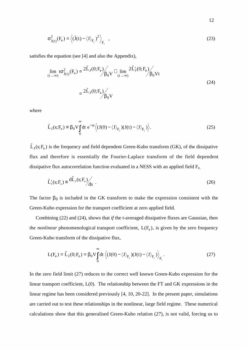
σJ t e F F

F J t Je

e( )

( ) ( ( ) )2 2= − , (23)

satisfies the equation (see [4] and also the Appendix),

lim ( )˜ ( ; ) lim

˜ ( ; )

˜ ( ; )

( ) ( ) ( )t J t eJ e

tJ e

J e

t F L FV

L FVt

L FV

→∞ →∞= + ′

=

σ β β

β

2

0 0

0

2 0 2 0

2 0

(24)

where

˜ ( ; ) ( ( ) )( ( ) )L s F V dt e J J J t JJ est

F Fe e≡ − −

∞−∫β0

0

0 . (25)

˜ ( ; )L s FJ e is the frequency and field dependent Green-Kubo transform (GK), of the dissipative

flux and therefore is essentially the Fourier-Laplace transform of the field dependent

dissipative flux autocorrelation function evaluated in a NESS with an applied field Fe.

˜ ( ; )˜ ( ; )′ ≡L s F dL s F

dsJ eJ e . (26)

The factor β0 is included in the GK transform to make the expression consistent with the

Green-Kubo expression for the transport coefficient at zero applied field.

Combining (22) and (24), shows that if the t-averaged dissipative fluxes are Gaussian, then

the nonlinear phenomenological transport coefficient, L Fe( ), is given by the zero frequency

Green-Kubo transform of the dissipative flux,

L F L F V dt J J J t Je J e F F Fe ee

( ) ˜ ( ; ) ( ( ) )( ( ) )= = − −∞

∫0 000

β . (27)

In the zero field limit (27) reduces to the correct well known Green-Kubo expression for the

linear transport coefficient, L(0). The relationship between the FT and GK expressions in the

linear regime has been considered previously [4, 10, 20-22]. In the present paper, simulations

are carried out to test these relationships in the nonlinear, large field regime. These numerical

calculations show that this generalised Green-Kubo relation (27), is not valid, forcing us to

12

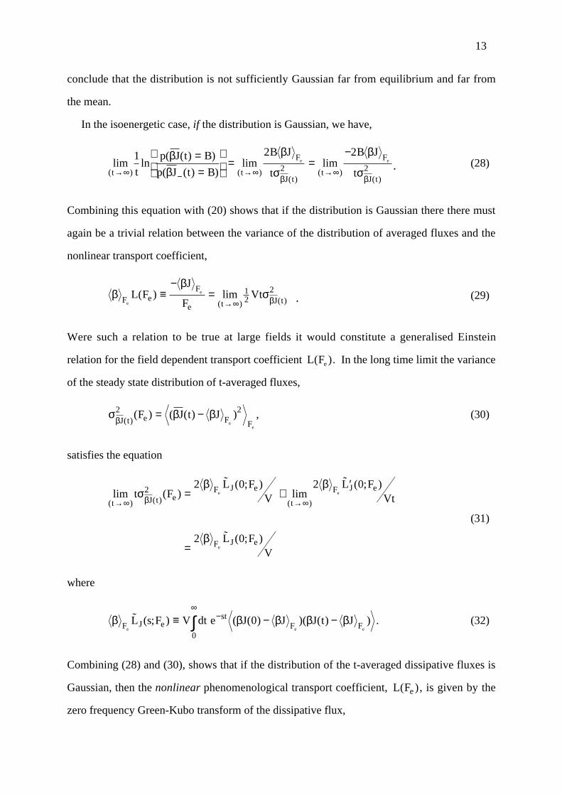
conclude that the distribution is not sufficiently Gaussian far from equilibrium and far from

the mean.

In the isoenergetic case, if the distribution is Gaussian, we have,

lim ln( ( ) )

( ( ) )lim lim

( ) ( )( )

( )( )

t t

F

J tt

F

J tt

p J t B

p J t B

B J

t

B J

te e

→∞ − →∞ →∞

==

= =

−1 2 22 2

ββ

β

σ

β

σβ β. (28)

Combining this equation with (20) shows that if the distribution is Gaussian there there must

again be a trivial relation between the variance of the distribution of averaged fluxes and the

nonlinear transport coefficient,

ββ

σβF eF

e t J te

eL FJ

FVt( ) lim

( ) ( )≡

−=

→∞12

2. (29)

Were such a relation to be true at large fields it would constitute a generalised Einstein

relation for the field dependent transport coefficient L Fe( ). In the long time limit the variance

of the steady state distribution of t-averaged fluxes,

σ β ββJ t e F FF J t J

ee

( )( ) ( ( ) )2 2= − , (30)

satisfies the equation

lim ( )˜ ( ; )

lim˜ ( ; )

˜ ( ; )

( ) ( ) ( )t J t eF J e

t

F J e

F J e

t FL F

VL F

Vt

L FV

e e

e

→∞ →∞= +

′

=

σβ β

β

β2 2 0 2 0

2 0

(31)

where

β β β β βF J est

F Fe e e

L s F V dt e J J J t J˜ ( ; ) ( ( ) )( ( ) )≡ − −∞

−∫0

0 . (32)

Combining (28) and (30), shows that if the distribution of the t-averaged dissipative fluxes is

Gaussian, then the nonlinear phenomenological transport coefficient, L Fe( ), is given by the

zero frequency Green-Kubo transform of the dissipative flux,

13

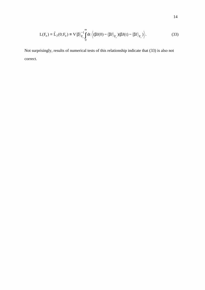
L F L F V dt J J J t Je J e F F Fe e e

( ) ˜ ( ; ) ( ( ) )( ( ) )= ≡ − −−∞

∫0 01

0

β β β β β . (33)

Not surprisingly, results of numerical tests of this relationship indicate that (33) is also not

correct.

14

V. NUMERICAL RESULTS

Steady state NEMD simulations of a fluid undergoing shear flow were used to test the

accuracy of the expressions derived above. All simulations were carried out in two Cartesian

dimensions with interactions between particles given by the Weeks-Chandler-Anderson

repulsive pair potential. Note that Lennard-Jones reduced units are used in the figures and

throughout this section. In both cases, simulations were carried out for systems of 200

particles and for the isokinetic system, the temperature was constrained at T = 1.0, whereas

for the isoenergetic system the internal energy was constrained at E/N = 1.56032. For the

isokinetic fluid, two densities, n=N/V, were considered: n = 0.4 and n = 0.8; and for the

isoenergetic fluid the density was set to n = 0.8.

The SLLOD equations of motion with Lees-Edwards periodic boundary conditions were

employed to model the shear flow, and a Gaussian thermostat or ergostat used to maintain a

steady state [16]. The adiabatic SLLOD equations give an exact representation of shear flow

arbitrarily far from equilibrium and Lees-Edwards periodic boundary conditions give the

unique generalisation of periodic boundary conditions to planar Couette flow. The SLLOD

equations (analogous to equation (1)) are given by:

˙

˙

q p i

p F i pi i i

i i yi i

y

p

= += − −

γγ α

(34)

where γ is the strain rate and α is the isokinetic or isoenergetic thermostat multiplier. When

the kinetic energy is a constant of motion,

αγ

K

i ii

N

xi yi

i ii

N

p p=

⋅ −

⋅

=

=

∑

∑

F p

p p

1

1

(35)

while if the internal energy is a constant of motion,

15

αγ

Exy

i ii

N

P V=

−

⋅=∑p p

1

(36)

where Pxy is the xy element of the pressure tensor,

P V p p x Fxy xi yii

N

ij yiji j

N

= −= =∑ ∑

1

12

1,, (37)

which is the dissipative flux: J ≡ Pxy. The nonlinear shear viscosity, η(γ) is the nonlinear

transport coefficient calculated using this algorithm. We note that in contrast to the

discussion above, the dissipative flux for shear flow is even under the time reversal mapping,

MT(x, y, px, py) = (x, y, - px, - py) and the strain rate is odd. However we can choose the

strain rate to be even and the dissipative flux odd by employing the Kawasaki mapping [16],

MK(x, y, px, py) = (x, -y, - px, py).

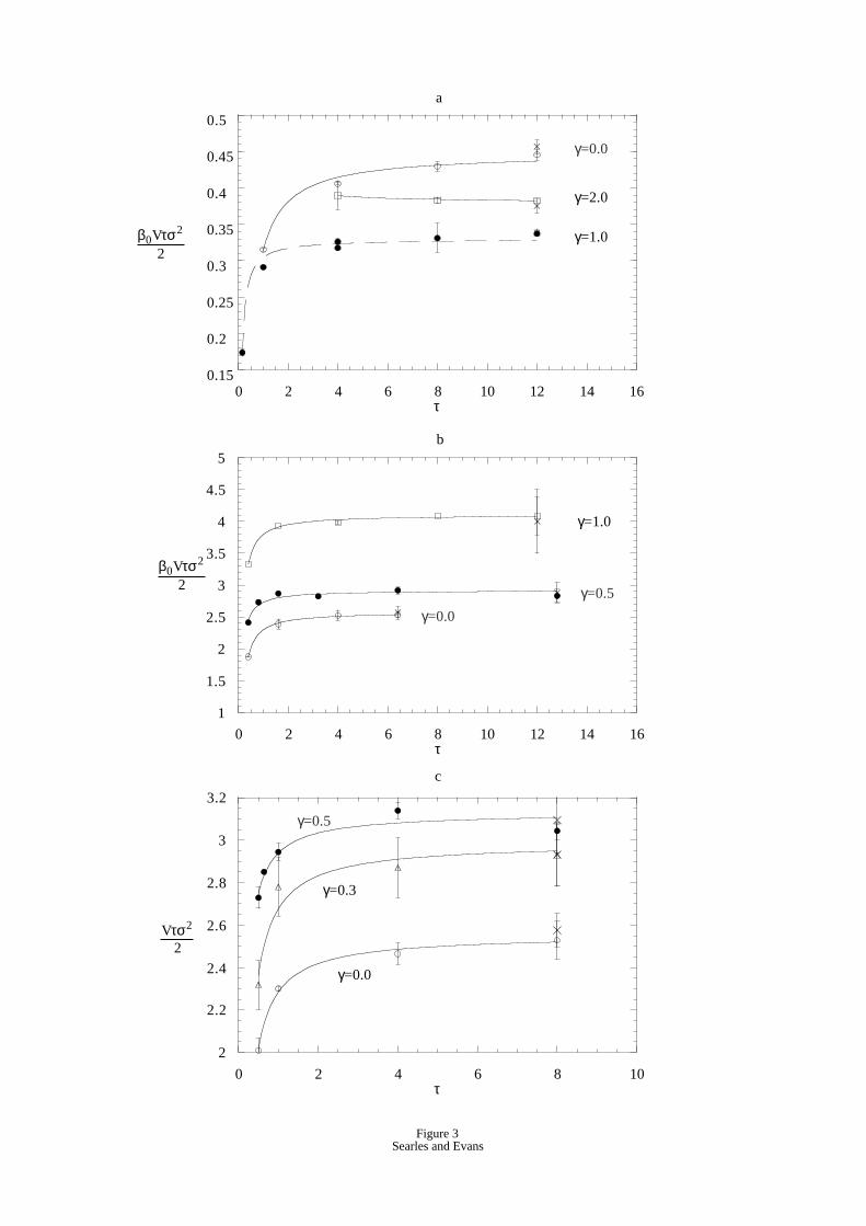
Firstly we carried out simulations to show that in the long time limit, for an isokinetic

system the variance of the distribution of {J t( )} is related to the zero frequency Green-Kubo

transform of J t( ) by equation (24), and for an isoenergetic system, the variance of the

distribution of {J tβ( )} is related to the zero frequency Green-Kubo transform of J tβ( ) by

equation (31). The behaviour at various strain rates was examined and the results are shown

in Figure 3. Equations (24) and (31) are found to be verified in all cases.

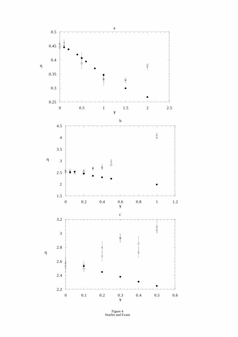
We tested the nonlinear Green-Kubo relations (27) and (33) for the systems described

above and the results are shown in Figure 4. Since L̃ (Fe) is also related to the variance of the

distribution of {J t( )} or { ( )}J tβ as t → ∞ for the isokinetic or isoenergetic system,

respectively, results obtained directly from the variance are also presented. Clearly the

equivalence of L(Fe) and L̃ (Fe) is only observed at small fields. At intermediate fields the

Green-Kubo transform of the dissipative flux L̃ (Fe), underestimates the actual transport

coefficient while at high fields ̃L Fe( ) , overestimates the transport coefficient. We conclude

that nonlinear Green-Kubo relations (27, 33) are not valid in the far from equilibrium regime.

16

VI. DISCUSSION

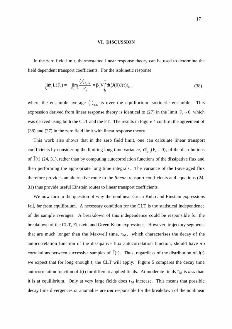
In the zero field limit, thermostatted linear response theory can be used to determine the

field dependent transport coefficients. For the isokinetic response:

lim ( ) lim ( ) ( ),

,Fe

F

F K

eK

e e

eL FJ

FV dt J J t

→ →

∞

= − = ∫0 00 0

0

0β (38)

where the ensemble average 0,K

is over the equilibrium isokinetic ensemble. This

expression derived from linear response theory is identical to (27) in the limit Fe→0, which

was derived using both the CLT and the FT. The results in Figure 4 confirm the agreement of

(38) and (27) in the zero field limit with linear response theory.

This work also shows that in the zero field limit, one can calculate linear transport

coefficients by considering the limiting long time variance, σJ t eF( )

( )2 0= , of the distributions

of J t( ) (24, 31), rather than by computing autocorrelation functions of the dissipative flux and

then performing the appropriate long time integrals. The variance of the t-averaged flux

therefore provides an alternative route to the linear transport coefficients and equations (24,

31) thus provide useful Einstein routes to linear transport coefficients.

We now turn to the question of why the nonlinear Green-Kubo and Einstein expressions

fail, far from equilibrium. A necessary condition for the CLT is the statistical independence

of the sample averages. A breakdown of this independence could be responsible for the

breakdown of the CLT, Einstein and Green-Kubo expressions. However, trajectory segments

that are much longer than the Maxwell time, τM , which characterises the decay of the

autocorrelation function of the dissipative flux autocorrelation function, should have no

correlations between successive samples of J t( ). Thus, regardless of the distribution of J(t)

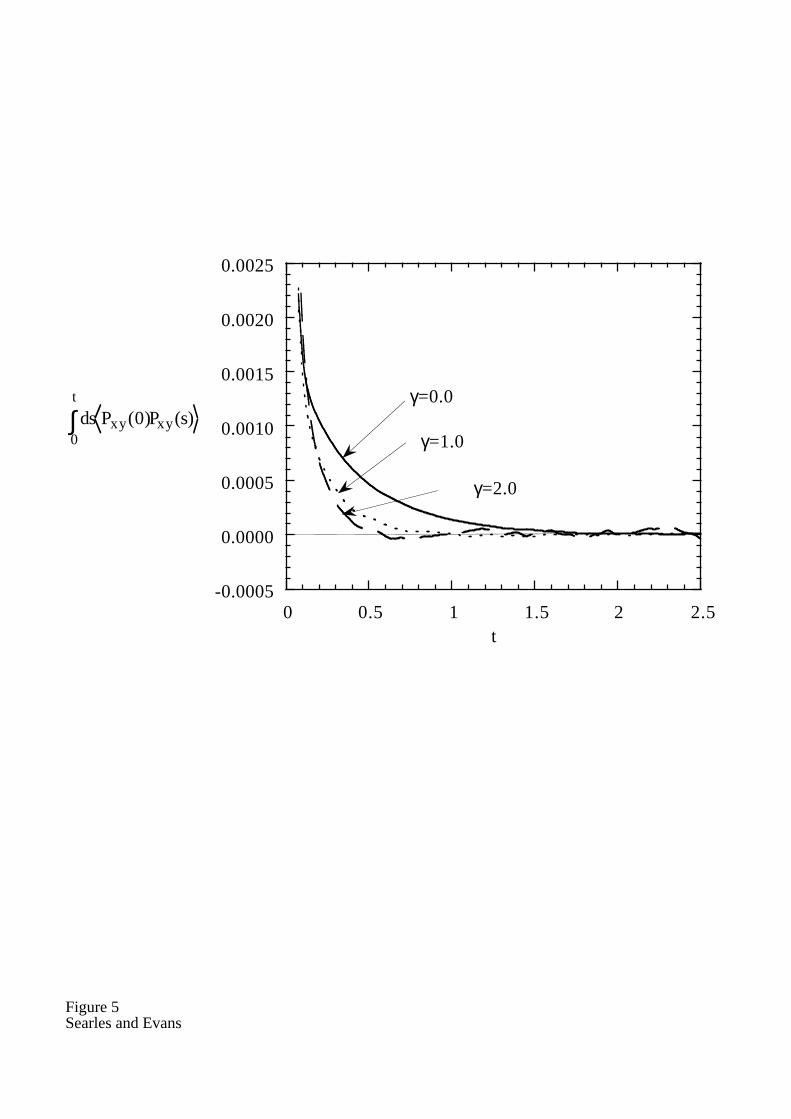
we expect that for long enough t, the CLT will apply. Figure 5 compares the decay time

autocorrelation function of J(t) for different applied fields. At moderate fields τM is less than

it is at equilibrium. Only at very large fields does τM increase. This means that possible

decay time divergences or anomalies are not responsible for the breakdown of the nonlinear

17

Einstein and GK expressions (33, 27). Further, if one computes the distribution of J t( ), for

various values of t, one cannot observe departures from Gaussian behaviour for values of t >>

τM, in the neighbourhood of the mean current.

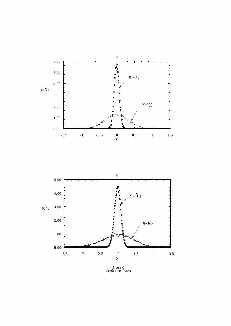
Figure 6 compares the distributions of J(t) (the distribution of the instantaneous flux) and

J t( ) for an equilibrium and nonequilibrium system with a strain rate which ensures it is in the

nonlinear regime (T=1.0, n=0.8, γ=1.0). While the skewness, γ1, and kurtosis, κ, for the

instantaneous equilibrium J(t) distribution are zero within error bars which is consistent with a

Gaussian distribution, the skewness is non-zero for the sheared system (γ1 = −0.23±0.01, κ =

0.13±0.04, respectively). The distributions of the time-averaged fluxes, J t( ), were obtained

for a trajectory segment of length t = 4.0 and both distributions, as expected, appear

Gaussian. The skewness of the distribution for the sheared system is γ1 = −0.064±0.004, and

the kurtosis κ = −0.02±0.02. Thus on the basis of these tests although for a sheared system

the distribution of J(t) is not Gaussian the distribution of J t( ), for a trajectory segment of

length t = 4.0, is on the scales shown in Figure 6, already indistinguishable from a Gaussian.

As noted in references [21, 22], the distribution of J t( ) and J tβ( ) cannot be exactly

Gaussian because the values of these variables are bounded. In practice however these

bounds are so large that they become irrelevant in the limit t → ∞ where the t-averaged

distributions collapse to zero variance distributions. Moreover, the bounds still apply in the

zero field limit where the Green-Kubo and Einstein expressions are all valid. Thus the

boundedness of the fluxes cannot be the responsible for the breakdown of the nonlinear GK

and Einstein expressions.

If we examine the derivation of equations (27) and (33) more closely, it can be seen that in

order to obtain a GK expression we require the distribution at both J t J t( ) ( )= + and

J t J t( ) ( )= − − be well approximated by a Gaussian for times sufficiently long that the GK

integrals have converged, t >> τM(Fe) (see Appendix for details) [13, 14]. Any deviations

from the behaviour indicated by (21) and (28) will be related to the relative deviation of the

distribution from a Gaussian at both J t+ ( ) and J t− ( ) . It is therefore of interest to consider the

18

rate of convergence to a Gaussian. The magnitude of the relative deviation of the distribution

p J t J J M

(( ( ) ) )( )− σ τ from a normalised Gaussian generally increases with the separation of

J t( ) from the mean J for sufficiently large separations (see, for example, section 7.2 of [13]).

Here σ τJ M( ) is the standard deviation of the distribution p J t( ( )) when t = τM . In the t → ∞

limit, at fixed J t( ), the magnitude of the relative devaition of p J t( ( )) from a Gaussian

becomes infinite. This means that in the t → ∞ limit, the CLT gives information which is not

sufficiently precise to derive Green-Kubo relations for non-zero applied fields.

We illustrate this point in more detail. Suppose that J t J t( ) ( )= + is equal to the mean

current, J; then the conjugate trajectories will have J t J t( ) ( )= − = − J. Clearly

| ( ) | ( )J t J L F Fe e− − = 2 . Therefore using equation (45) of Appendix A, we find in the t → ∞

limit, except when Fe = 0,

J t J L F F F VtL FJ e e J e eM M

− − = ≈ → ∞( ) / ( ) / ( )( ) ( )σ σ βτ τ2 2 . (39)

For any non zero field, if J t( )= J, then as t increases, the value of J t− ( ) moves further and

further into the wings of the normalised distribution where the magnitude of the relative

deviation of p J t( ( )) from a Gaussian grows without bound. Strictly speaking therefore, in the

infinite time limit, for any finite field, the relative deviation of p J t( ( )) from a Gaussian,

evaluated in the neighbourhood of the mean anticurrent, − J grows without bound and

nonlinear Green-Kubo relations cannot be derived. However, in practice one does not need to

take the infinite time limit. Considering the shift in the mean value of the dissipative flux

with field shows that the nonlinear GK expression will be approximately correct provided,

F V F L Fe M M e e≤ ( )Ο 1 / ( ) ( )β τ , (40)

where VM is the minimum volume required for transport coefficient to be approximately

equal to its large system, limiting value [24]. Clearly the nonlinear GK relations satisfy this

relation only in a small neighbourhood including Fe = 0. For the systems studied here,

equation (40) predicts that the nonlinear GK relations will be approximately correct provided

19

γ < −~ 10 1. This is in agreement with experimental observations given in Figures 4(a),(b),

4(c).

20

Acknowledgements

We would like to thank the Australian Research Council for the support of this project. The

helpful discussions and comments from Professor E.G.D. Cohen, Professor G. Gallavotti, Dr

C. Jarzynski and Dr R. van Zon are also gratefully acknowledged. DJE would like to thank

the National Institute of Standards and Technology, Boulder, Colorado for support.

References

[1] D. J. Evans, E. G. D. Cohen and G. P. Morriss, Phys. Rev. Lett., 71, 2401 (1993).

[2] J-P. Eckmann and I. Procaccia, Phys. Rev. A, 34, 659 (1986).

[3] D. J. Evans and D. J. Searles, Phys. Rev. E, 50, 1645 (1994).

[4] D. J. Evans and D. J. Searles, Phys. Rev. E, 52, 5839 (1995).

[5] D. J. Evans and D. J. Searles, Phys. Rev. E, 53, 5808 (1996).

[6] G. Gallavotti and E. G. D. Cohen, J. Stat. Phys., 80, 931 (1995).

[7] G. Gallavotti and E. G. D. Cohen, Phys. Rev. Letts., 74, 2694 (1995).

[8] G. Ayton and D. J. Evans, J. Stat. Phys., 97, 811 (1999); E. G. D. Cohen and G.

Gallavotti, J. Stat. Phys., 96, 1343 (1999).

[9] D. J. Searles and D. J. Evans, Phys. Rev. E, 60, 159 (1999).

[10] J. L. Lebowitz and H. Spohn, J. Stat. Phys., 95, 333 (1999).

[11] J. Kurchan, J. Phys. A, 31, 3719 (1998).

[12] C. Maes, J. Stat. Phys., 95, 367 (1999).

[13] H. Cramér, Mathematical methods of statistics, (Princeton University Press, Princeton,

1966).

[14] H. Cramér, Random variables and probability distributions, (Cambridge University

Press, London, 1970); B. V. Gnedenko and A. N. Kolmogorov, Limit distributions for

sums of independent random variables, (Addison-Wesley, Massachusetts, 1954).

[15] CLT states that under quite general conditions [13, 14], the mean of an infinite set of

independent variables is normally distributed, independent of the distribution of the

individual independent variables. However, for a finite number of variables, unless the

21

independent variables are distributed as a Gaussian, the sum will show some deviation

from a Gaussian and the relative error in the deviation will generally increase with the

number of standard deviations from the mean when the number of variables is large [13,

14] .

[16] D. J. Evans and G. P. Morriss, Statistical Mechanics of Nonequilibrium Liquids

(Academic Press, London, 1990).

[17] D. J. Searles and D. J. Evans, "Ensemble dependence of the transient fluctuation

theorem", http://xxx.lanl.gov/abs/cond-mat/9906002.

[18] Note that a Gaussian distribution does not imply a FT. The FT is a much stronger

statement: it specifies the relationship between the mean and the standard deviation if

the distribution is Gaussian. We note that the FT of course, does not require the

distribution to be Gaussian.

[19] D. J. Evans and G. P. Morriss, Phys. Rev. A, 31, 3817 (1985).

[20] G. Gallavotti, Phys. Rev. Letts, 77, 4334 (1996).

[21] F. Bonetto, G. Gallavotti and P. L. Garrido, Physica D, 105, 226 (1997).

[22] F. Bonetto, N. I. Chernov and J. L. Lebowitz, Chaos, 8, 823 (1998).

[23] We assume that the FT and equations (23) and (30) have reached their limiting

behaviour at that time.

[24] A similar argument can be used if we take the thermodynamic limit, in which the

distribution collapses onto a delta function at the mean. In this case a GK expression is

valid for large systems provided the distribution of the time-averaged fluxes is Gaussian

at a minimal volume.

22

Appendix.

The variance of the time-averaged dissipative flux is given by,

σJ t

t t

tt

J t J

tds J s ds J s

tds ds J s J s

( )( ( ) )

( ) ( )

( ) ( )

2 2

2 1 10 2 20

2 1 20 1 20

1

1

= −

= ( )( )=

∫ ∫

∫∫

∆ ∆

∆ ∆

(40)

where ∆J t J t J( ) ( )= − . Using a change of variables: τ1 1 2= −s s and τ2 1 2= +s s this

integral can be written:

σ τ τ τ τ τ

τ τ τ τ τ τ τ

τ

τ

τ

τ

J t

t

t

td ds J J

td ds J J

( )( ( )) ( ( ))

( ( )) ( ( ))

22 2 2

12 1 2

12 2 10

2 2 212 1 2

12 2 10

121

2

2

2

2

2

= + −

+ + − − −

−

−

∫∫

∫∫

∆ ∆

∆ ∆(41)

Since correlation functions are invariant under a time translation in the steady state, and

using the symmetry of the functions we obtain,

σ τ τ τJ t

tt

td d J J

( )( ) ( )2

2 2 1 100

20= ∫∫ ∆ ∆ . (42)

Changing the order of integration gives:

σ τ τ τ

τ τ τ

τ τ τ

τ

τ

J t

tt

tt

t

td d J J

td d J J

td J J t

( )( ) ( )

( ) ( )

( ) ( )( )

22 1 2 10

2 1 2 10

2 1 1 10

20

20

20

1

1

=

=

= −

∫∫

∫∫

∫

∆ ∆

∆ ∆

∆ ∆

. (43)

Therefore, for any steady state system, at all times:

t F ds J J J s Jt

ds J J J s J sJ t e

t

F F

t

F Fe e e eσ

( )( ) ( ( ) )( ( ) ) ( ( ) )( ( ) )2

0 02 0

20= − − − − −∫ ∫ . (44)

At any time greater than the time required for the time correlation function to decay to zero,

tC > tM, in an isokinetic system, ds J J J s J L F Vt

F F J e

C

e e0 00 0∫ − − =( ( ) )( ( ) ) ˜ ( ; ) / ( )β and

ds J J J s J s L s F Vt

F F J e

C

e e0 00∫ − − = − ′( ( ) )( ( ) ) ˜ ( ; ) / ( )β . Therefore,

23

t F L FV

L FVtC J t e

J e J e

CCσ β β( )

( )˜ ( ; ) ˜ ( ; )2

0 0

2 0 2 0= + ′. (45)

If the distribution is Gaussian at J t( ) and -J t( ) at tC, then assuming that the second term of

(45) is negligible and that the FT is true at t = tC, combining (20) and (45) gives,

−= =

J

FVt L FF

eC J t J e

e

C

12 0

2 0β σ( )

˜ ( ; ). (46)

That is, a GK expression is valid.

24

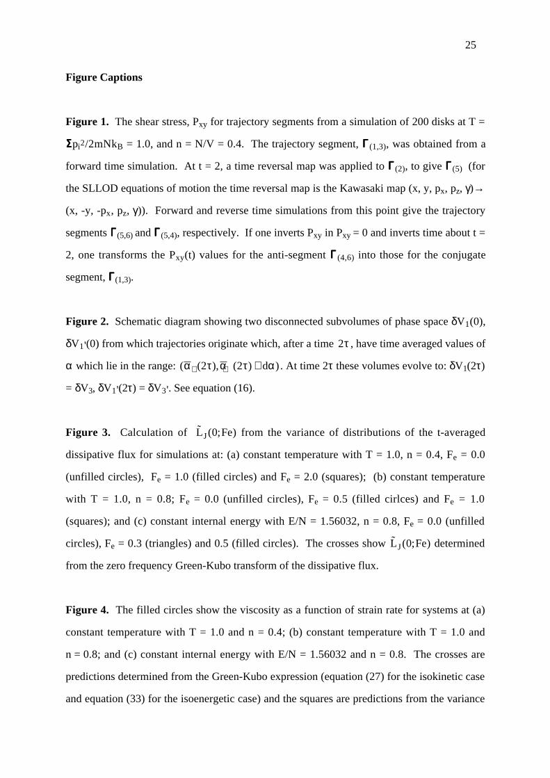
Figure Captions

Figure 1. The shear stress, Pxy for trajectory segments from a simulation of 200 disks at T =

Spi2/2mNkB = 1.0, and n = N/V = 0.4. The trajectory segment, G(1,3), was obtained from a

forward time simulation. At t = 2, a time reversal map was applied to G(2), to give G(5) (for

the SLLOD equations of motion the time reversal map is the Kawasaki map (x, y, px, pz, γ)→

(x, -y, -px, pz, γ)). Forward and reverse time simulations from this point give the trajectory

segments G(5,6) and G(5,4), respectively. If one inverts Pxy in Pxy = 0 and inverts time about t =

2, one transforms the Pxy(t) values for the anti-segment G(4,6) into those for the conjugate

segment, G(1,3).

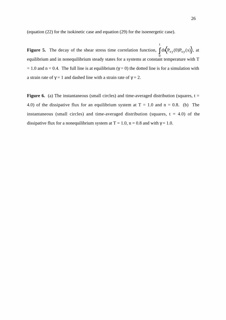
Figure 2. Schematic diagram showing two disconnected subvolumes of phase space δV1(0),

δV1'(0) from which trajectories originate which, after a time 2τ , have time averaged values of

α which lie in the range: ( ( ), ( ) )α τ α τ α+ + +2 2 d . At time 2τ these volumes evolve to: δV1(2τ)

= δV3, δV1'(2τ) = δV3'. See equation (16).

Figure 3. Calculation of ˜ ( ; )L FeJ 0 from the variance of distributions of the t-averaged

dissipative flux for simulations at: (a) constant temperature with T = 1.0, n = 0.4, Fe = 0.0

(unfilled circles), Fe = 1.0 (filled circles) and Fe = 2.0 (squares); (b) constant temperature

with T = 1.0, n = 0.8; Fe = 0.0 (unfilled circles), Fe = 0.5 (filled cirlces) and Fe = 1.0

(squares); and (c) constant internal energy with E/N = 1.56032, n = 0.8, Fe = 0.0 (unfilled

circles), Fe = 0.3 (triangles) and 0.5 (filled circles). The crosses show ˜ ( ; )L FeJ 0 determined

from the zero frequency Green-Kubo transform of the dissipative flux.

Figure 4. The filled circles show the viscosity as a function of strain rate for systems at (a)

constant temperature with T = 1.0 and n = 0.4; (b) constant temperature with T = 1.0 and

n = 0.8; and (c) constant internal energy with E/N = 1.56032 and n = 0.8. The crosses are

predictions determined from the Green-Kubo expression (equation (27) for the isokinetic case

and equation (33) for the isoenergetic case) and the squares are predictions from the variance

25

(equation (22) for the isokinetic case and equation (29) for the isoenergetic case).

Figure 5. The decay of the shear stress time correlation function, ds Pxy(0)Pxy(s)0

t

∫ , at

equilibrium and in nonequilibrium steady states for a systems at constant temperature with T

= 1.0 and n = 0.4. The full line is at equilibrium (γ = 0) the dotted line is for a simulation with

a strain rate of γ = 1 and dashed line with a strain rate of γ = 2.

Figure 6. (a) The instantaneous (small circles) and time-averaged distribution (squares, t =

4.0) of the dissipative flux for an equilibrium system at T = 1.0 and n = 0.8. (b) The

instantaneous (small circles) and time-averaged distribution (squares, t = 4.0) of the

dissipative flux for a nonequilibrium system at T = 1.0, n = 0.8 and with γ = 1.0.

26

-0.8

-0.6

-0.4

-0.2

0.0

0.2

0.4

0.6

0.8

0 0.5 1 1.5 2 2.5 3 3.5 4

Px y

t

(1)

(2)(3)

(5)

(6)

(4)

Γ(5)

=M(K)Γ(2)

τ 2τ

Figure 1Searles and Evans

δV1δV3

δV1' δV3'

α τ τ α τ ατ τ

+ = =∫ ∫( ) ( ; ) ( ; )'2 12

120

21 0

21dt t dt tΓΓ ΓΓ

Figure 2Searles and Evans

δδ

δδ τα τV

VV

V N3

1

3

16 2= = − +

'

'exp[ ( )]

2

2.2

2.4

2.6

2.8

3

3.2

0 2 4 6 8 10τ

γ=0.5

γ=0.3

γ=0.0

Vτσ2

2

Figure 3Searles and Evans

c

1

1.5

2

2.5

3

3.5

4

4.5

5

0 2 4 6 8 10 12 14 16τ

γ=0.5

γ=1.0

γ=0.0

β0Vτσ2

2

b

0.15

0.2

0.25

0.3

0.35

0.4

0.45

0.5

0 2 4 6 8 10 12 14 16τ

γ=1.0

γ=0.0

γ=2.0

β0Vτσ2

2

a

2.2

2.4

2.6

2.8

3

3.2

0 0.1 0.2 0.3 0.4 0.5 0.6

η

γ

Figure 4Searles and Evans

c

1.5

2

2.5

3

3.5

4

4.5

0 0.2 0.4 0.6 0.8 1 1.2

η

γ

b

0.25

0.3

0.35

0.4

0.45

0.5

0 0.5 1 1.5 2 2.5

η

γ

a

-0.0005

0.0000

0.0005

0.0010

0.0015

0.0020

0.0025

0 0.5 1 1.5 2 2.5t

γ=0.0

γ=1.0

γ=2.0

Figure 5Searles and Evans

dsPxy(0)Pxy(s)0

t

∫

0.00

1.00

2.00

3.00

4.00

5.00

-3.5 -3 -2.5 -2 -1.5 -1 -0.5X

X=J(t)

p(X)

X = J (t)

Figure 6Searles and Evans

b

0.00

1.00

2.00

3.00

4.00

5.00

6.00

-1.5 -1 -0.5 0 0.5 1 1.5X

X=J(t)

p(X)

X = J (t)

a