The Force Method 9...The Force Method 9 Abstract Up to this point, we have focused on the analysis of statically determinate structures because the analysis process is fairly straightforward;

The Force Method 9

Abstract

Up to this point, we have focused on the analysis of statically determinate

structures because the analysis process is fairly straightforward; only the

force equilibrium equations are required to determine the member forces.

However, there is another category of structures, called statically indeter-

minate structures, which are also employed in practice. Indeterminate

structures require another set of equations, in addition to the force equi-

librium equations, in order to solve for the member forces. There are two

general methods for analyzing indeterminate structures, the force (flexi-

bility) method and the displacement (stiffness) method. The force method

is more suited to hand computation whereas the displacement method is

more procedural and easily automated using a digital computer.

In this chapter, we present the underlying theory of the force method

and illustrate its applications to a range of statically indeterminate

structures including trusses, multi-span beams, arches, and frames. We

revisit the analysis of these structures in the next chapter using the

displacement method, and also in Chap. 12, “Finite Element Displace-

ment Method for Framed Structures,” which deals with computer-based

analysis.

9.1 Introduction

The force method is a procedure for analyzing statically indeterminate structures that works with

force quantities as the primary variables. It is applicable for linear elastic structures. The method is

based on superimposing structural displacement profiles to satisfy a set of displacement constraints.

From a historical perspective, the force method was the “classical” analysis tool prior to the

introduction of digital-based methods. The method is qualitative in the sense that one reasons

about deflected shapes and visualizes how they can be combined to satisfy the displacement

constraints. We find the method very convenient for deriving analytical solutions that allow one to

identify key behavior properties and to assess their influence on the structural response. The key step

# Springer International Publishing Switzerland 2016

J.J. Connor, S. Faraji, Fundamentals of Structural Engineering,DOI 10.1007/978-3-319-24331-3_9

561

http://dx.doi.org/10.1007/978-3-319-24331-3_12

is establishing the displacement constraints which are referred to as the geometric compatibility

equations.

Consider the structure shown in Fig. 9.1. Since there are four displacement restraints, the structure

is indeterminate to the first degree, i.e., one of the restraints is not needed for stability, and the

corresponding reaction force cannot be determined using only the force equilibrium equations.

The steps involved in applying the force method to this structure are as follows:

1. We select one of the force redundants and remove it. The resulting structure, shown in Fig. 9.2, is

called the primary structure. Note that one cannot arbitrarily remove a restraint. One needs to

ensure that the resulting structure is stable.

2. We apply the external loading to the primary structure and determinate the displacement at C in

the direction of the restraint at C. This quantity is designated as ΔC, 0. Figure 9.3 illustrates this

notation.

3. Next, we apply a unit value of the reaction force at C to the primary structure and determine the

corresponding displacement. We designate this quantity as δCC (see Fig. 9.4).

4. We obtain the total displacement at C of the primary structure by superimposing the displacement

profiles generated by the external loading and the reaction force at C.

ΔC

��primary structure ¼ ΔC, 0 þ δCCRC ð9:1Þ

5. The key step is to require the displacement at C of the primary structure to be equal to the

displacement at C of the actual structure.

Fig. 9.1 Actual structure

Fig. 9.2 Primary structure

562 9 The Force Method

ΔC

��actual ¼ ΔC

��primary ¼ ΔC,0 þ δCCRC ð9:2Þ

Equation (9.2) is referred to as the “geometric compatibility equation.” When this equation is

satisfied, the final displacement profiles for the actual and the primary structure will be identical. It

follows that the forces in the primary structure and the actual structure will also be identical.

6. We solve the compatibility equation for the reaction force, RC.

RC ¼ 1

δCCΔC

��actual � ΔC,0

� � ð9:3Þ

Note that ΔC

��actual ¼ 0 when the support is unyielding. When RC is negative, the sense assumed in

Fig. 9.4 needs to be reversed.

7. The last step involves computing the member forces in the actual structure. We superimpose the

member forces computed using the primary structure according to the following algorithm:

Force ¼ Force��external load þ RC Force

��RC¼1

� � ð9:4Þ

Since the primary structure is statically determinate, all the material presented in Chaps. 2, 3, 4, 5,

and 6 is applicable. The force method involves scaling and superimposing displacement profiles. The

method is particularly appealing for those who have a solid understanding of structural behavior. For

simple structures, one can establish the sense of the redundant force through qualitative reasoning.

Fig. 9.3 Displacements

due to the external loading

Fig. 9.4 Displacement

due to unit value of RC

9.1 Introduction 563

http://dx.doi.org/10.1007/978-3-319-24331-3_2

http://dx.doi.org/10.1007/978-3-319-24331-3_3

http://dx.doi.org/10.1007/978-3-319-24331-3_4

http://dx.doi.org/10.1007/978-3-319-24331-3_5

http://dx.doi.org/10.1007/978-3-319-24331-3_6

Essentially, the same approach is followed for structures having more than one degree of

indeterminacy. For example, consider the structure shown in Fig. 9.5. There are two excess vertical

restraints.

We obtain a primary structure by removing two of the vertical restraints. Note that there are

multiple options for choosing the restraints to be removed. The only constraint is that the primary

structure must be “stable.” Figure 9.6 shows the different choices.

Suppose we select the restraints at C and D as the redundants. We apply the external loading to the

primary structure (Fig. 9.7) and determine the vertical displacements at C and D shown in Fig. 9.8.

The next step involves applying unit forces corresponding to RC ¼ 1 and RD ¼ 1 and computing

the corresponding displacements at C and D. Two separate displacement analysis are required since

there are two redundant reactions (Fig. 9.9).

Combining the three displacement profiles leads to the total displacement of the primary structure.

ΔC

��primary structure ¼ ΔC,0 þ δCCRC þ δCDRD

ΔD

��primary structure ¼ ΔD,0 þ δDCRC þ δDDRD

ð9:5Þ

The coefficients of RC and RD are called flexibility coefficients. It is convenient to shift over to

matrix notation at this point. We define

Δ0 ¼ΔC, 0

ΔD, 0

( )X ¼

RC

RD

( )

flexibility matrix ¼ δ ¼δCC δCD

δDC δDD

" # ð9:6Þ

Using this notation; the geometric compatibility equation takes the form

Δ��actual structure ¼ Δ0 þ δX ð9:7Þ

Note that Δ��actual structure ¼ 0 when the supports are unyielding. Given the choice of primary

structure, the flexibility coefficients are properties of the primary structure whereas Δ0 depends on

the both the external loading and the primary structure. We solve (9.7) for X,

Fig. 9.5 Actual structure


Fig. 9.6 Choices for

primary structure. (a)Option 1. (b) Option 2.

(c) Option 3

Fig. 9.7 Primary structure


X ¼ δ�1 Δ��actual structure � Δ0

� � ð9:8Þ

and then determine the member forces by superimposing the individual force states as follows:

F ¼ F��external load þ F

��RC¼1

� �RC þ F

��RD¼1

� �RD ð9:9Þ

The extension of this approach to an nth degree statically indeterminate structure just involves

more computation since the individual matrices are now of order n. Since there are more redundant

force quantities, we need to introduce a more systematic notation for the force and displacement

quantities.

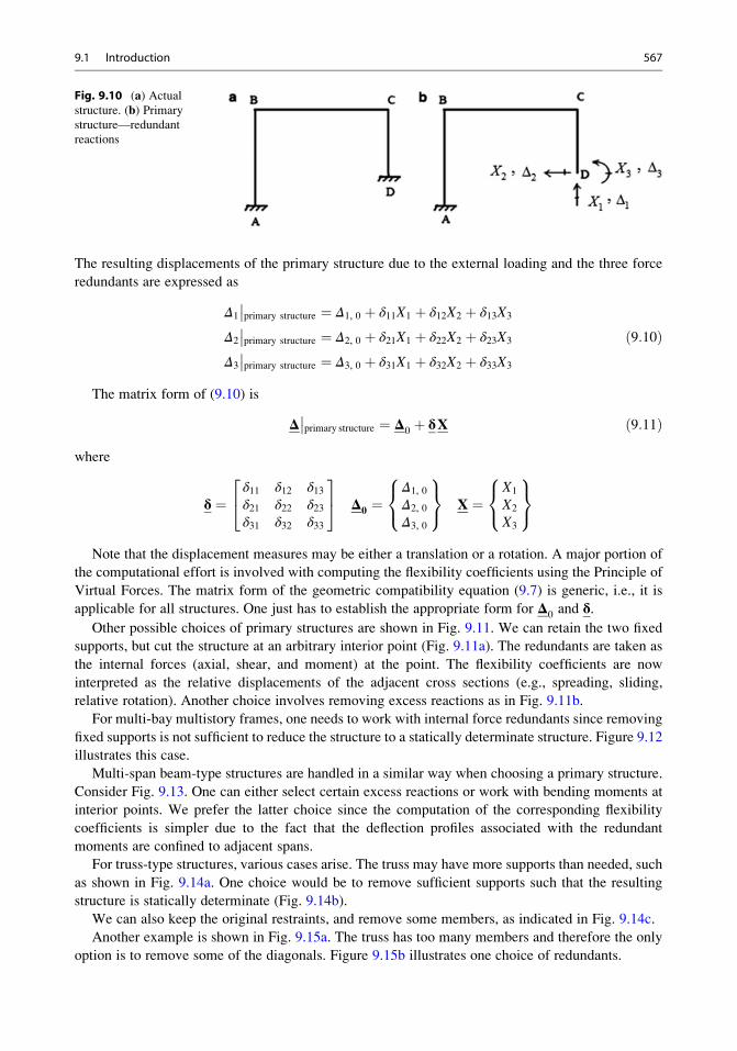
Consider the frame structure shown in Fig. 9.10a. It is indeterminate to the third degree. One

choice of primary structure is shown in Fig. 9.10b. We remove the support at D, take the reactions as

the force redundants, and denote the jth redundant force as Xj and the corresponding measure as Δj.

Fig. 9.8 Displacements

due to external loading

Fig. 9.9 Displacement

due to unit values of the

redundant. (a) RC ¼ 1.

(b) RD ¼ 1


The resulting displacements of the primary structure due to the external loading and the three force

redundants are expressed as

Δ1

��primary structure ¼ Δ1, 0 þ δ11X1 þ δ12X2 þ δ13X3

Δ2


Δ3


ð9:10Þ

The matrix form of (9.10) is

Δ��primary structure ¼ Δ0 þ δX ð9:11Þ

where

δ ¼δ11 δ12 δ13δ21 δ22 δ23δ31 δ32 δ33

24

35 Δ0 ¼

Δ1, 0

Δ2, 0

Δ3, 0

8<:

9=; X ¼

X1

X2

X3

8<:

9=;

Note that the displacement measures may be either a translation or a rotation. A major portion of

the computational effort is involved with computing the flexibility coefficients using the Principle of

Virtual Forces. The matrix form of the geometric compatibility equation (9.7) is generic, i.e., it is

applicable for all structures. One just has to establish the appropriate form for Δ0 and δ.Other possible choices of primary structures are shown in Fig. 9.11. We can retain the two fixed

supports, but cut the structure at an arbitrary interior point (Fig. 9.11a). The redundants are taken as

the internal forces (axial, shear, and moment) at the point. The flexibility coefficients are now

interpreted as the relative displacements of the adjacent cross sections (e.g., spreading, sliding,

relative rotation). Another choice involves removing excess reactions as in Fig. 9.11b.

For multi-bay multistory frames, one needs to work with internal force redundants since removing

fixed supports is not sufficient to reduce the structure to a statically determinate structure. Figure 9.12

illustrates this case.

Multi-span beam-type structures are handled in a similar way when choosing a primary structure.

Consider Fig. 9.13. One can either select certain excess reactions or work with bending moments at

interior points. We prefer the latter choice since the computation of the corresponding flexibility

coefficients is simpler due to the fact that the deflection profiles associated with the redundant

moments are confined to adjacent spans.

For truss-type structures, various cases arise. The truss may have more supports than needed, such

as shown in Fig. 9.14a. One choice would be to remove sufficient supports such that the resulting

structure is statically determinate (Fig. 9.14b).

We can also keep the original restraints, and remove some members, as indicated in Fig. 9.14c.

Another example is shown in Fig. 9.15a. The truss has too many members and therefore the only

option is to remove some of the diagonals. Figure 9.15b illustrates one choice of redundants.

Fig. 9.10 (a) Actualstructure. (b) Primary

structure—redundant

reactions



structure

Fig. 9.11 (a) Primary


internal forces. (b) Primary


reactions

Fig. 9.13 Multi-span

beam. (a) Actual structure.(b) Primary structure—

redundant reactions. (c)Primary structure—

redundant moments


9.2 Maxwell’s Law of Reciprocal Displacements

The geometric compatibility equations involve the flexibility matrix,δ. One computes the elements of

δusing one of the methods described in Part I, such as the Principal of Virtual Forces. Assuming there

are n force redundants, δ has n2 elements. For large n, this computation task becomes too difficult to

deal with manually. However, there is a very useful relationship between the elements of δ, called“Maxwell’s Law,” which reduces the computational effort by approximately 50 %. In what follows,

we introduce Maxwell’s Law specialized for member systems.

We consider first a simply supported beam on unyielding supports subjected to a single

concentrated unit force. Figure 9.16a defines the geometry and notation. The deflected shape due to



reactions. (c) Primary


internal forces



internal forces

9.2 Maxwell’s Law of Reciprocal Displacements 569

the unit force applied at A is plotted in Fig. 9.16b. Suppose we want to determine the deflection at B

due to this load applied at A. We define this quantity as δBA. Using the Principle of Virtual Forces

specialized for beam bending; we apply a unit virtual force at B (see Fig. 9.16c) and evaluate the

following integral:

δBA ¼ðMAδMB

dx

EIð9:12Þ

where MA is the moment due to the unit load applied at A, and δMB is the moment due to the virtual

unit load applied at B.

Fig. 9.16 Reciprocal

loading conditions. (a)Actual structure. (b) Actualloading (MA). (c) Virtualloading (δMB). (d) Actualloading (MB). (e) Virtualloading (δMA)


Now, suppose we want the deflection at A due to a unit load at B. The corresponding virtual force

expression is

δAB ¼ðMBδMA

dx

EIð9:13Þ

where δMA is the virtual moment due to a unit force applied at A and MB is the moment due to the

load at B. Since we are applying unit loads, it follows that

MA ¼ δMA

MB ¼ δMB

ð9:14Þ

and we find that the expressions for δAB and δBA are identical.

δAB�δBA ð9:15ÞThis identity is called Maxwell’s Law. It is applicable for linear elastic structures [1]. Returning

back to the compatibility equations, defined by (9.7), we note that the coupling terms, δij and δji, areequal. We say the coefficients are symmetrical with respect to their subscripts and it follows that δis symmetrical. Maxwell’s Law leads to another result called Muller–Breslau Principle which is

used to establish influence lines for indeterminate beams and frames. This topic is discussed in

Chaps. 13 and 15.

9.3 Application of the Force Method to Beam-Type Structures

We apply the theory presented in the previous section to a set of beam-type structures. For

completeness, we also include a discussion of some approximate techniques for analyzing partially

restrained single-span beams that are also useful for analyzing frames.

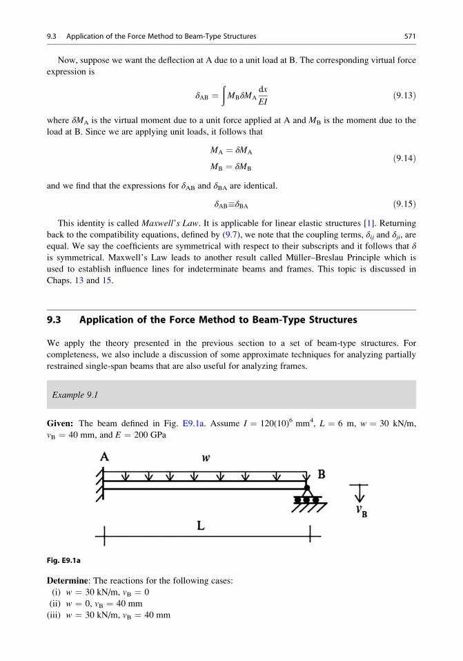
Example 9.1

Given: The beam defined in Fig. E9.1a. Assume I ¼ 120(10)6 mm4, L ¼ 6 m, w ¼ 30 kN/m,

vB ¼ 40 mm, and E ¼ 200 GPa

Fig. E9.1a

Determine: The reactions for the following cases:

(i) w ¼ 30 kN/m, vB ¼ 0

(ii) w ¼ 0, vB ¼ 40 mm

(iii) w ¼ 30 kN/m, vB ¼ 40 mm

9.3 Application of the Force Method to Beam-Type Structures 571

http://dx.doi.org/10.1007/978-3-319-24331-3_13

http://dx.doi.org/10.1007/978-3-319-24331-3_15

Solution: The beam is indeterminate to the first degree. We work with the primary structure shown

below (Fig. E9.1b).

Fig. E9.1b Primary structure

Applying the external loading and the unit load results in the following deflected shapes

(Figs. E9.1c and E9.1d):

Fig. E9.1c Displacement due to external loading

Fig. E9.1d Displacement due to the unit values of RB The deflection terms are given in Table 3.1.

ΔB,0 ¼ wL4

8EI#

δBB ¼ L3

3EI"

Then

þ " ΔB

��actual ¼ ΔB,0 þ δBBRB

+

ΔB

��actual ¼ �wL4

8EIþ L3

3EIRB ∴ RB ¼ ΔB

��actual þ wL4=8EI

� �L3=3EI� �


http://dx.doi.org/10.1007/978-3-319-24331-3_3

Case (i): For ΔB

��actual ¼ 0

RB ¼ wL4=8EI� �

= L3=3EI� �� ¼ 3

8wL ¼ 3

830ð Þ 6ð Þ ¼ 67:5kN "

Knowing the value of RB, we determine the remaining reactions by using the static equilibrium

equations.

XFy ¼ 0 RA ¼ 5

8wL ¼ 5

830ð Þ 6ð Þ ¼ 112:5kN "

XM@A ¼ 0 MA ¼ wL2

8¼ 135kNm counterclockwise

Case (ii): For w ¼ 0, ΔB|actual ¼ –vB

RB ¼ �vBð ÞL3=3EI� � ¼ � 3EI

L3vB¼ � 3 200ð Þ 10ð Þ6120 10ð Þ�6

6ð Þ3 0:040ð Þ ¼ �13:33kN ∴ RB ¼ 13:33kN #

The reactions are

XFy ¼ 0 RA ¼ 3EI

L3vB ¼ 13:3kN "X

M@A ¼ 0 MA ¼ 3EI

L2vB ¼ 80kNm counterclockwise

Case (iii): For w 6¼ 0 and ΔB

��actual ¼ –vB

RB ¼ �vB þ wL4=8EI� �

L3=3EI� � ¼ þ3

8wL� 3EI

L3vB ¼ 67:5� 13:33 ¼ 54:2kN "


The reactions are as follows:

Note that since the structure is linear, one can superimpose the solutions for cases (i) and (ii).

Example 9.2

Given: The beam and loading defined in Fig. E9.2a. Assume I ¼ 400 in.4, L ¼ 54 ft, w ¼ 2.1 kip/ft,

δA ¼ 2.4 in., and E ¼ 29,000 ksi.

Fig. E9.2a

Determine: The reactions due to

(i) The distributed load shown

(ii) The support settlement at A

Solution: The beam is indeterminate to the first degree. We take the vertical reaction at B as the force

unknown and compute the deflected shapes due to w and RB ¼ 1 applied to the primary structure

(Figs. E9.2b and E9.2c).

Fig. E9.2b Deflected shape due to w

Fig. E9.2c Deflected shape due to unit value of RB


Case (i): The distributed load shown

þ " ΔB


+ΔB,0 þ δBBRB ¼ 0 ∴ RB ¼ �ΔB,0

δBB

The deflection terms can be determined using (3.34).

ΔB,0 ¼ � 4wL4

729EI

δBB ¼ 4L3

243EI

Then

RB ¼ �ΔB,0

δBB¼ 4wL4=729EI� �4L3=243EI� � ¼ wL

3¼ 37:8kip "

Knowing the value of RB, we determine the remaining reactions by using the static equilibrium

equations.

Case (ii): The support settlement at A (Fig. E9.2d)

Fig. E9.2d Displacement due to support settlement at A

þ " ΔB


where

δBB ¼ 4L3

243EI¼ 4 54ð Þ3 12ð Þ3

243 29; 000ð Þ 400ð Þ ¼ 0:386 in:

ΔB,0 ¼ 2

3δA ¼ �1:6 in:


http://dx.doi.org/10.1007/978-3-319-24331-3_3

Therefore

RB ¼ �ΔB,0

δBB¼ � �1:6ð Þ

0:386¼ 4:14kip "

We determine the remaining reactions using the static equilibrium equations.

Example 9.3

Given:

The three-span beam defined in Fig. E9.3a. Assume EI is constant, L ¼ 9 m, and w ¼ 20 kN.

Fig. E9.3a

Determine: The reactions

Solution: The beam is indeterminate to the second degree. We remove the supports at B and C, take

the vertical reactions at B and C as the force redundants, and compute the deflected shapes due to w,

X1 ¼ 1, and X2 ¼ 1 applied to the primary structure (Figs. E9.3b, E9.3c, E9.3d).

Fig. E9.3b Deflected shape due to external loading

Fig. E9.3c Deflected shape due to X1 ¼ 1


Fig. E9.3d Deflected shape due to X2 ¼ 1

The displacements of the primary structure due to the external loading and the two force

redundants are expressed as:

Δ1,0 þ δ11X1 þ δ12X2 ¼ 0

Δ2,0 þ δ21X1 þ δ22X2 ¼ 0

Noting symmetry and the deflection results listed in Table 3.1, it follows that:

X1 ¼ X2

Δ1,0 ¼ Δ2,0 ¼ � 11wL4

12EI

δ11 ¼ δ22 ¼ 4L3

9EI

δ21 ¼ δ12 ¼ 7L3

18EI

Then

X1 ¼ X2 ¼ �Δ1,0

δ11 þ δ12¼ 11wL4=12EI

� �4L3=9EI� �þ 7L3=18EI

� � ¼ 1:1wL ¼ 1:1 20ð Þ 9ð Þ ¼ 198kN

Lastly, we determine the remaining reactionsXFY ¼ 0 RA ¼ RD ¼ 0:4wL ¼ 72kN "

9.3.1 Beam with Yielding Supports

We consider next the case where a beam is supported by another member, such as another beam

or a cable. Examples are shown in Fig. 9.17. When the beam is loaded, reactions are developed,

and the supporting members deform. Assuming linear elastic behavior, the supporting members


http://dx.doi.org/10.1007/978-3-319-24331-3_3

behave as linear elastic restraints, and can be modeled as equivalent spring elements, as indicated in

Fig. 9.17.

We consider here the case where a vertical restraint is provided by another beam. Figure 9.18

illustrates this case. Point B is supported by beam CD which is parallel to beam AB. In this case, point

B deflects when the load is applied to beam AB. One strategy is to work with a primary structure that

includes both beams such as shown in Fig. 9.19. The force redundant is now a pair of self-

equilibrating forces acting at B, and the corresponding displacement measure is the relative displace-

ment apart between the upper and lower contact points, designated as B and B0.

Fig. 9.17 Beam on

flexible supports. (a) Beam.

(b) Cable. (c) Column

Fig. 9.18 Beam supported

by another beam


The total displacement corresponding to X1 ¼ 1 is the sum of two terms,

δ11 ¼ δ11��AB þ δ11

��CD

¼ L3

3EIþ δ11

��CD

Beam CD functions as a restraint on the movement of beam AB. The downward movement of B0 isresisted by the bending action of beam CD. Assuming linear elastic behavior, this restraint can be

modeled as a linear spring of stiffness k. One chooses the magnitude of k such that the spring

deflection due to the load P is the same as the beam deflection.

Then, it follows from Fig. 9.20 that

δ11

��CD ¼ 1

kCDð9:16Þ

Assuming the two beams are rigidly connected at B, the net relative displacement must be zero.

Δ1 ¼ Δ1,0 þ X1

1

kCDþ L3

3EI

� �¼ 0 ð9:17Þ

Fig. 9.19 Choice of force

redundant and

displacement profiles. (a)Primary structure—force

redundant system. (b)Deflection due to external

loading. (c) Deflection due

to redundant force at B


Solving (9.17) for X1 leads to

X1 ¼ �1

L3=3EI� �þ 1=kCDð Þ

( )Δ1,0 ð9:18Þ

Note that the value of X1 depends on the stiffness of beam CD. Taking kCD ¼ 1 corresponds to

assuming a rigid support, i.e., a roller support. When kCD ¼ 0, X1 ¼ 0. It follows that the bounds

on X1 are

0 < X1 <3EI

L3

� �Δ1,0 ð9:19Þ

When the loading is uniform,

Δ1,0 ¼ wL4

8EI#

Another type of elastic restraint is produced by a cable. Figure 9.21 illustrates this case. We replace

the cable with its equivalent stiffness, kC ¼ AcEc

h and work with the primary structure shown in

Fig. 9.21b.

Using the results derived above, and noting that Δ1 ¼ 0, the geometric compatibility equation is

Δ1 ¼ Δ1,0 þ δ11��AB þ δ11

��BC

� �X1 ¼ 0

For the external concentrated loading,

Δ1,0 ¼ P

EI

a2L

2� a3

3

� �

Fig. 9.20 Equivalent spring


Substituting for the various flexibility terms leads to

X1 ¼ �1

L3=3EbIb� �þ 1=kcð Þ

" #Δ1,0 ð9:20Þ

If 1kcis small with respect to L3

3EbIb, the cable acts like a rigid support, i.e., X1 approaches the value

for a rigid support. When 1kcis large with respect to L3

3EbIb, the cable is flexible and provides essentially

no resistance, i.e., X1 ) 0. The ratio of cable to beam flexibilities is a key parameter for the behavior

of this system.

Cable-stayed schemes are composed of beams supported with inclined cables. Figure 9.22a shows

the case where there is just one cable. We follow essentially the same approach as described earlier


structure—force redundant

system. (c) Deflection due

to applied load


except that now the cable is inclined. We take the cable force as the redundant and work with the

structure defined in Fig. 9.22b.

Note that Δ1 is the relative movement together of points B and B0 along the inclined direction. Up

to this point, we have been working with vertical displacements. Now we need to project these

movements on an inclined direction.

We start with the displacement profile shown in Fig. 9.22c. The vertical deflection is vB0.Projecting on the direction of the cable leads to

Fig. 9.22 (a) Cable-stayed scheme. (b) Forceredundant. (c) Deflectiondue to applied load. (d)Deflection due to X1 ¼ 1.

(e) Displacement

components


Δ1,0 ¼ � sin θvB0 ¼ � sin θP

EBIB

a2LB2

� a3

6

� �� ð9:21Þ

Next, we treat the case where X1 ¼ 1 shown in Fig. 9.22d. The total movement consists of the

elongation of the cable and the displacement of the beam.

δ11 ¼ δ11��BC þ δ11

��AB

The elongation of the cable is

δ11��BC ¼ Lc

ACEC

¼ 1

kC

The beam displacement follows from Fig. 9.22e.

δ11��AB ¼ vB,1 sin θ ¼ sin θ

sin θL3B3EBIB

� �¼ sin θð Þ2 L3B

3EBIB

� �

Requiring Δ1 ¼ 0 leads to

X1 ¼ 1

sin θð Þ2 L3B=3EBIB� �þ 1=kCð Þ

P sin θ

EBIB

a2LB2

� a3

6

� � ð9:22Þ

Finally, we express X1 in terms of the value of the vertical reaction corresponding to a rigid

support at B.

X1 ¼ sin θ

sin θð Þ2 þ 3 EBIB=L3B

� �LC=ECACð ÞR

��rigid support at B ð9:23Þ

There are two geometric parameters, θ, and the ratio of IB/LB3 to AC/LC. Note that X1 varies with

the angle θ. When cables are used to stiffen beams, such as for cable-stayed bridges, the optimum

cable angle is approximately 45�. The effective stiffness provided by the cable degrades rapidly withdecreasing θ.

Example 9.4

Given: The structure defined in Fig. E9.4a.

Assume I ¼ 400 in.4, L ¼ 54 ft, w ¼ 2.1 kip/ft, kv ¼ 25 kip/in., and E ¼ 29,000 ksi.

Determine: The reactions, the axial force in the spring, and the displacement at B.

Fig. E9.4a


Solution: The structure is indeterminate to the first degree. We take the axial force in the spring at B

as the force unknown.

The geometric compatibility equation is

Δ1,0 þ δ11jABC þ 1

kv

� �X1 ¼ 0

The deflection terms can be determined using (3.34).

Δ1,0 ¼ � 4wL4

729EI¼ 14:6 in:

δ11

��ABC ¼ 4L3

243EI¼ 0:386 in:

Fig. E9.4b Deflected shape due to X1 ¼ 1

Fig. E9.4c Deflected shape due to external loading

Solving for X1, leads to:


http://dx.doi.org/10.1007/978-3-319-24331-3_3

X1 ¼ Δ1,0

δ11

��ABC þ 1=kvð Þ ¼14:6

0:386þ 1=25ð Þ ¼ 34:26kip "

The displacement at B is

vB ¼ X1

kv¼ 34:26

25¼ 1:37 in: #

Next, we determine the remaining reactions by using the static equilibrium equations.

Example 9.5

Given: The structure defined in Fig. E9.5a. Assume I ¼ 200(10)6 mm4, L ¼ 18 m, P ¼ 45 kN,

AC ¼ 1300 mm2, and E ¼ 200 GPa.

Fig. E9.5a

Determine: The forces in the cables, the reactions, and the vertical displacement at the intersection of

the cable and the beam.


(a) θ ¼ 45�

(b) θ ¼ 15�

Solution: The structure is indeterminate to the second degree. We take the cable forces as the force

redundants and work with the structure defined below (Fig. E9.5b).


Next, we compute the deflected shapes due to external loading P, X1 ¼ 1, and X2 ¼ 1 applied to

the primary structure (Figs. E9.5c, E9.5d, E9.5e).

Fig. E9.5c External loading P

Fig. E9.5d X1 ¼ 1

Fig. E9.5e X2 ¼ 1

The displacements of the primary structure due to the external loading and the two force

redundants are expressed as


Δ1,0 þ δ11X1 þ δ12X2 ¼ 0

Δ2,0 þ δ21X1 þ δ22X2 ¼ 0

where

δ11 ¼ δ11jBeam þ δ11jcableδ22 ¼ δ22jBeam þ δ22jcableδ12 ¼ δ12jBeamδ21 ¼ δ21jBeam

also

Δ1,0 ¼ vB,0 sin θ

Δ2,0 ¼ vC,0 sin θ

δ11jBeam ¼ vB,1 sin θ

δ21jBeam ¼ vC,1 sin θ

δ21jBeam ¼ vB,2 sin θ

δ22jBeam ¼ vC,2 sin θ

Because of symmetry:

δ11��Beam ¼ δ22

��Beam ¼ vB,1 sin θ ¼ 3 sin θ2L3

256EI

δ12��Beam ¼ δ21

��Beam ¼ vB,2 sin θ ¼ 7 sin θ2L3

768EI

Δ1,0 ¼ Δ2,0 ¼ vB,0 sin θ ¼ 11 sin θPL3

768EI

δ11��Cable ¼ δ22

��Cable ¼ LC

ACE¼ L

4 cos θACE

X1 ¼ X2

Lastly, the redundant forces are

X1 ¼ X2 ¼ Δ1,0

δ11��Beam þ δ11

��Cable

� �þ δ12��Beam


(a) For θ ¼ 45�

X1 ¼ X2 ¼ Δ1,0


��Cable


¼ 43kN

∴ 2X1 sin θ ¼ 2 43ð Þ sin 45 ¼ 60:8kN

The remaining reactions are determined using the static equilibrium equations.

(b) For θ ¼ 15�

X1 ¼ X2 ¼ Δ1,0


��Cable


¼ 109:8kN

∴ 2X1 sin θ ¼ 2 109:8ð Þ sin 15 ¼ 56:9kN

The remaining reactions are determined using the static equilibrium equations.

9.3.2 Fixed-Ended Beams

We treat next the beam shown in Fig. 9.23a. The structure is fully restrained at each end and therefore

is indeterminate to the second degree. We take as force redundants the counterclockwise end

moments at each end. The corresponding displacement measures are the counterclockwise end

rotations, θA and θB.We write the general form of the compatibility equations as (we use θ instead of Δ to denote the

displacement measures and M instead of X for the force measures):


θA ¼ θA,0 þMAθAA þMBθAB

θB ¼ θB,0 þMAθBA þMBθBBð9:24Þ

where θA,0 and θB,0 depend on the nature of the applied loading, and the other flexibility coefficients

are

θAA ¼ L

3EI

θBB ¼ L

3EI

θAB ¼ θBA ¼ � L

6EI

We solve (9.24) for MA and MB

MA ¼ 2EI

L2 θA � θA,0ð Þ þ θB � θB,0ð Þf g

MB ¼ 2EI

L2 θB � θB,0ð Þ þ θA � θA,0ð Þf g

ð9:25Þ

When the ends are fixed, θA ¼ θB ¼ 0, and the corresponding values ofMA andMB are called the

fixed end moments. They are usually denoted as MAF and MB

F

Fig. 9.23 (a) Beam with

full end restraint. (b)Primary structure. (c)External loading—

displacement profile. (d)Displacement profile for

MA ¼ 1. (e) Displacement

profile for MB ¼ 1


M FA ¼ � 2EI

L2θA,0 þ θB,0f g

M FB ¼ � 2EI

L2θB,0 þ θA,0f g

ð9:26Þ

Introducing this notation in (9.25), the expressions for the end moments reduce to

MA ¼ 2EI

L2θA þ θBf g þM F

A

MB ¼ 2EI

L2θB þ θAf g þM F

B

ð9:27Þ

We will utilize these equations in Chap. 10.

Example 9.6 Fixed End Moments for Uniformly Distributed Loading

Given: The uniform distributed loading applied to a fixed end beam (Fig. E9.6a).

Fig. E9.6a

Determine: The fixed end moments.

Solution: We take the end moments at A and B as force redundant (Fig. E9.6b).


Noting Table 3.1, the rotations due to the applied load are (Fig. E9.6c)

EIθA,0 ¼ �wL3

24EIθB,0 ¼ wL3

24


http://dx.doi.org/10.1007/978-3-319-24331-3_10

http://dx.doi.org/10.1007/978-3-319-24331-3_3

Fig. E9.6c Deformation of primary structure due to applied load

Substituting their values in (9.26) leads to

M FA ¼ � 2EI

L2θA,0 þ θB,0f g ¼ wL2

6� wL2

12¼ wL2

12

M FB ¼ � 2EI

L2θB,0 þ θA,0f g ¼ �wL2

6þ wL2

12¼ �wL2

12

2FA

2FB

wLM

12wL

M12

=

=

The shear and moment diagrams are plotted in Fig. E9.6d.

Fig. E9.6d

Note that the peak positive moment for the simply supported case is +(wL2/8). Points of inflectionare located symmetrically at


x ¼ L

21� 1ffiffiffi

3p

� �� 0:21L

This solution applies for full fixity. When the member is part of a frame, the restraint is provided

by the adjacent members, and the end moments will generally be less than the fully fixed value.

Example 9.7 Fixed End Moment—Single Concentrated Force

Given: A single concentrated force applied at an arbitrary point x ¼ a on the fixed end beam shown

in Fig. E9.7a.

Fig. E9.7a

Determine: The fixed end moments.

Solution: We work with the primary structure defined in Fig. E9.7b.


Using the results listed in Table 3.1, the rotations are given by (Fig. E9.7c)

EIθA,0 ¼ �Pa L� að Þ 2L� að Þ6L

EIθB,0 ¼ Pa L� að Þ Lþ að Þ6L

Fig. E9.7c Deformation of primary structure due to external loading


http://dx.doi.org/10.1007/978-3-319-24331-3_3

Substituting into (9.26) leads to

M FA ¼ Pa L� að Þ2

L2

M FB ¼ �P L� að Þa2

L2

The critical location for maximum fixed end moment is a ¼ L/2; the corresponding maximum

values are M FA ¼ �M F

B ¼ PL8. The shear and moment diagrams are plotted below.

Note that there is a 50 % reduction in peak moment due to end fixity.

Results for various loadings and end conditions are summarized in Tables 9.1 and 9.2.


Table 9.1 Fixed end actions for fully fixed


9.3.3 Analytical Solutions for Multi-Span Beams

Consider the two-span beam shown in Fig. 9.24a. We allow for different lengths and different

moments of inertia for the spans. Our objective here is to determine analytically how the maximum

positive and negative moments vary as the load moves across the total span. We choose the negative

moment at B as the redundant. The corresponding primary structure is shown in Fig. 9.24b. Here,ΔθBis the relative rotation together of adjacent cross sections at B.

The geometric compatibility equation involves the relative rotation at B.

ΔθB ¼ ΔθB,0 þ δθBBMB ¼ 0

The various rotation terms are given in Table 3.1. Note that the δθBB term is independent of the

applied loading.

δθBB ¼ 1

3E

L1I1

þ L2I2

� �

When the loading is on span AB (see Table 3.1),

ΔθB,0 ¼ � P

6EI1L1a a2 � L21� �

Table 9.2 Fixed end actions for partially fixed


http://dx.doi.org/10.1007/978-3-319-24331-3_3

http://dx.doi.org/10.1007/978-3-319-24331-3_3

Then

MB ¼ �ΔθB,0δθBB

¼ L1=I1ð ÞL1=I1ð Þ þ L2=I2ð Þ

� �1

2Pa 1� a2

L12

� �ð9:28Þ

Given the value of MB, we can determine the reactions by using the static equilibrium equations.

Noting (9.28), the peak moments are given by:

Negativemoment MB ¼ �PL12

fa

L11� a2

L12

� �

Positivemoment MD ¼ PL1a

L1

� �1� a

L1

� �� f

2

a2

L211� a2

L21

� �� ð9:29Þ

where

f ¼ 1

1þ I1=L1ð Þ L2=I2ð Þ

Fig. 9.24 (a) Actualstructure—notation for

a two-span beam. (b)Primary structure—

redundant moment. (c)Displacement due to a unit

value of the redundant

moment. (d) Rotation due

to external loading


We define the ratio of I to L as the “relative stiffness” for a span and denote this parameter by r.

ri ¼ I

L

��span i

ð9:30Þ

With this notation, f takes the form

f ¼ 1

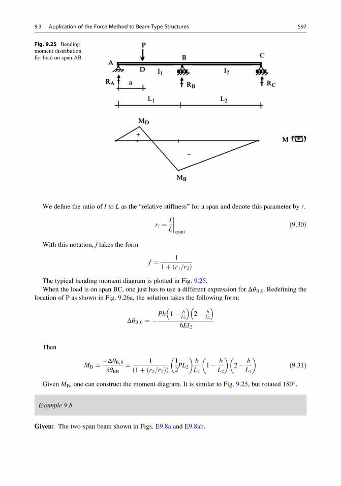
1þ r1=r2ð ÞThe typical bending moment diagram is plotted in Fig. 9.25.

When the load is on span BC, one just has to use a different expression for ΔθB,0. Redefining the

location of P as shown in Fig. 9.26a, the solution takes the following form:

ΔθB,0 ¼ �Pb 1� b

L2

� 2� b

L2

� 6EI2

Then


¼ 1

1þ r2=r1ð Þð Þ1

2PL2

� �b

L21� b

L2

� �2� b

L2

� �ð9:31Þ

Given MB, one can construct the moment diagram. It is similar to Fig. 9.25, but rotated 180�.

Example 9.8

Given: The two-span beam shown in Figs. E9.8a and E9.8ab.

Fig. 9.25 Bending

moment distribution

for load on span AB


Fig. 9.26 (a) Actualstructure—loading on span

BC. (b) Primary


moment. (c) Rotation due

to external loading. (d)Bending moment

distribution for load on

span BC


Determine: The variation of the bending moment at B with relative stiffness of the adjacent spans (r1/

r2 ¼ 0.1, 1, and 10).

Fig. E9.8a

Fig. E9.8b

Solution: We determine the variation of the moment at B for a range of relative stiffness ratios

covering the spectrum from one span being very flexible to one span being very rigid with respect to

the other span using (9.29) and (9.31). Results for the individual spans are plotted in Figs. E9.8c and

E9.8d.

Fig. E9.8c Load on the left span (9.29)


Fig. E9.8d Load on the right span (9.31)

Example 9.9 Two-Span Continuous Beam—Uniform Loading

Given: The two-span beam shown in Fig. E9.9a.

Fig. E9.9a

Determine: The bending moment at support B.

Solution: We take the negative moment at the interior support as the force redundant. The solution

process is similar to that followed for the case of a concentrated load. One determines the relative

rotations at B, and then enforces continuity at B (Fig. E9.9b).

Fig. E9.9b


The various terms are (see Table 3.1)

ΔθB,0 ¼ � w1L31

24EI1� w2L

32

24EI2

δθBB ¼ L13EI1

þ L23EI2

Requiring the relative rotation at B equal to zero leads to


¼ w1L21

8

� �1þ w2=w1ð Þ L2=L1ð Þ2 r1=r2ð Þ

1þ r1=r2ð Þwhere

r1 ¼ I1L1

, r2 ¼ I2L2

Suppose the loading and span lengths are equal. In this case,

MB ¼ wL2

8

for all combinations of I1 and I2. The moment diagram is plotted below (Fig. E9.9c).

Fig. E9.9c

Another interesting case is where w2 ¼ 0 and I1 ¼ I2. The solution depends on the ratio of span

lengths.

MB ¼ w1L12

8

1

1þ L2=L1ð Þ


http://dx.doi.org/10.1007/978-3-319-24331-3_3

Suppose L2 ¼ L1 and I1 ¼ I2, then

MB ¼ 1

2

w1L12

8

� �

Example 9.10 Two-Span Continuous Beam with Support Settlement

Given: The two-span beam shown in Fig. E9.10a. The supports at B or A experience a vertical

displacement downward due to settlement of the soil under the support.

Fig. E9.10a

Determine: The bending moment at B.

Solution: We work with the primary structure shown in Fig. E9.10b.

Fig. E9.10b Primary structure—redundant moment

If the support at B moves downward an amount vB, the relative rotation of the section at B is

ΔθB,0 ¼ vBL1

þ vBL2


Compatibility requires the moment at B to be equal to


¼ � vB 1=L1ð Þ þ 1=L2ð Þð Þ1=3Eð Þ L1=I1ð Þ þ L2=I2ð Þð Þ

The minus sign indicates that the bending moment is of opposite sense to that assumed in

Fig. E9.10b.

When the properties are the same for both spans (I1 ¼ I2 and L1 ¼ L2), MB reduces to

MB ¼ 3EI1

L21vB.

When the support at A moves downward an amount vA, the behavior is reversed.

In this case, ΔθB,0 ¼ �vA=L1 and MB ¼ vA=L11=3Eð Þ L1=I1ð Þ þ L2=I2ð Þð Þ

When the properties are the same for both spans (I1 ¼ I2 and L1 ¼ L2), MB reduces to

MB ¼ 3EI1

2L21vA.

9.4 Application to Arch-Type Structures

Chapter 6 introduced the topic of arch structures. The discussion was concerned with how the

geometry of arch structures is defined and how to formulate the equilibrium equations for statically

determinate arches. Various examples were presented to illustrate how arch structures carry

9.4 Application to Arch-Type Structures 603

http://dx.doi.org/10.1007/978-3-319-24331-3_6

transverse loading by a combination of both axial and bending actions. This feature makes them more

efficient than beam structures for long-span applications.

In what follows we extend the analytical formulation to statically indeterminate arches. We base

our analysis procedure on the force method and use the principle of virtual forces to compute

displacement measures. One of our objectives here is to develop a strategy for finding the geometry

for which there is minimal bending moment in the arch due to a particular loading.

We consider the two-hinged arch shown in Fig. 9.27a. This structure is indeterminate to the first

degree. We take the horizontal reaction at the right support as the force redundant and use the

Principle of Virtual Forces described in Sect. 6.5 to determine Δ1,0, the horizontal displacement due to

loading, and δ11, the horizontal displacement due to a unit value of X1.

The general expressions for these displacement measures follow from (6.9)

Δ1,0 ¼ðs

F0

AEδFþ V0 xð Þ

GAs

δV þM0 xð ÞEI

δM

� �ds

δ11 ¼ðs

δFð Þ2AE

þ δVð Þ2GAs

þ δMð Þ2EI

( )ds

ð9:32Þ

We usually neglect the shear deformation term. Whether one can also neglect the axial deforma-

tion term depends on the arch geometry. For completeness, we will retain this term. The two internal

force systems are summarized below. We assume the applied load is uniform per projected length

(Fig. 9.28).

Substituting for the force terms leads to the following expressions for the displacement measures:

Δ1,0 ¼ð L0

1

AE cos θ

wL

2� wx

� �sin θ cos θ þ tan α sin θð Þ � wL

2x� wx2

2

� �Δy

EI cos θ

� �dxδ11

¼ð L0

cos θ þ tan α sin θð Þ2AE cos θ

þ Δyð Þ2EI cos θ

( )dx

ð9:33Þ

Fig. 9.27 (a) Actualstructure—geometry. (b)Primary structure—

redundant reaction


http://dx.doi.org/10.1007/978-3-319-24331-3_6

http://dx.doi.org/10.1007/978-3-319-24331-3_6

Geometric compatibility requires

X1 ¼ �Δ1,0

δ11ð9:34Þ

One can use either symbolic integration or numerical integration to evaluate the flexibility

coefficients. We prefer to use the numerical integration scheme described in Sect. 3.6.6.

The solution simplifies considerably when axial deformation is neglected with respect to bending

deformation. One sets A ¼ 1 in (9.33). This leads to

Δ1,0 ¼ �ðL0

wL

2x� wx2

2

� �Δy

EI cos θdx ¼ �

ðL0

M0ΔyEI cos θ

dx

δ11 ¼ þðL0

Δyð Þ2EI cos θ

dx

ð9:35Þ

Suppose Δy is chosen such that

Δy ¼ βwL

2x� wx2

2

�βM0 ð9:36Þ

Then,

Δ1,0 ¼ �1

βδ11

and it follows that

X1 ¼ 1

β

M¼ M0 þ X1δM ¼ M0 þ 1

β

� ��βM0ð Þ ¼ 0

ð9:37Þ

Fig. 9.28 (a) Force due toapplied loading (F0, M0).

(b) Force due to X1 ¼ 1

(δF, δM)


http://dx.doi.org/10.1007/978-3-319-24331-3_3

With this choice of geometry, the arch carries the exterior load by axial action only; there is no

bending. Note that this result is based on the assumption that axial deformation is negligible. In

general, there will be a small amount of bending when h is not small with respect to L, i.e., when the

arch is “shallow.” One cannot neglect axial deformation for a shallow arch.

Example 9.11 Parabolic Arch with Uniform Vertical Loading

Given: The two-hinged parabolic arch defined in Fig. E9.11a.

Fig. E9.11a

Determine: The bending moment distribution.

Solution: The centroidal axis for the arch is defined by

y ¼ 4hx

L� x

L

� 2

The bending moment in the primary structure due to the uniform loading per unit x is

M0 ¼ wL

2x� wx2

2¼ wL2

2

x

L� x

L

� 2

We note that the expressions for y andM0 are similar in form. One is a scaled version of the other.

M0 ¼ wL2

2

1

4hy ¼ wL2

8hy

Then, noting (9.36),

β ¼ 8h

wL2

and X1 ¼ wL2

8h.


The total moment is the sum of M0 and the moment due to X1.

M ¼ M0 � yX1 ¼ wL2

8hy� wL2

8hy ¼ 0

We see that there is no bending for this loading and geometry. We should have anticipated this result

since a uniformly loaded cable assumes a parabolic shape. By definition, a cable has no bending

rigidity and therefore no moment. We can consider an arch as an inverted cable. It follows that a

two-hinged uniformly loaded parabolic arch behaves like an inverted cable.

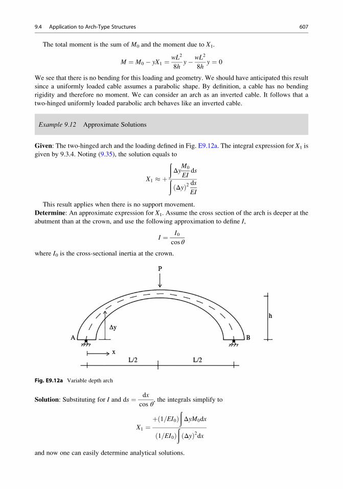
Example 9.12 Approximate Solutions

Given: The two-hinged arch and the loading defined in Fig. E9.12a. The integral expression for X1 is

given by 9.3.4. Noting (9.35), the solution equals to

X1 � þ

ðΔy

M0

EIdsð

Δyð Þ2 dsEI

This result applies when there is no support movement.

Determine: An approximate expression for X1. Assume the cross section of the arch is deeper at the

abutment than at the crown, and use the following approximation to define I,

I ¼ I0cos θ

where I0 is the cross-sectional inertia at the crown.

Fig. E9.12a Variable depth arch

Solution: Substituting for I and ds ¼ dx

cos θ, the integrals simplify to

X1 ¼þ 1=EI0ð Þ

ðΔyM0dx

1=EI0ð Þð

Δyð Þ2dx

and now one can easily determine analytical solutions.


Suppose a concentrated force, P, is applied at mid-span. The corresponding terms for a symmetri-

cal parabolic arch are:

Δy ¼ 4y

Lx� x2

L

� �1

EI0

ðΔyM0dx ) 5

48

PhL2

EI01

EI0

ðΔyð Þ2dx ¼ 8

15

h2L

EI0

X1 ¼ 25

128P

L

h

� �

Note that the bending moment is not zero in this case.

Example 9.13

Given: The two-hinged arch and the loading defined in Fig. E9.13a

Fig. E9.13a

Determine: The particular shape of the arch which corresponds to negligible bending.

Solution: This two-hinged arch is indeterminate to the first degree. We take the horizontal reaction at

the right support as the force redundant (Fig. E9.13b).


Fig. E9.13b Primary structure—redundant reaction

The applied loading is given by (Fig. E9.13c)

w xð Þ ¼ w0 2:5� 1:5

50x

� �0 < x � 50

Fig. E9.13c

The corresponding shear and moment in the simply supported beam spanning AB are

dV

dx¼ w xð Þ ) V ¼ w0 2:5x� 1:5

100x2

� �þ C1

dM

dx¼ �V ) M ¼ �w0

2:5

2x2 � 1:5

300x3

� �þ C1xþ C2

Enforcing the boundary conditions,

M 0ð Þ ¼ 0

M 100ð Þ ¼ 0

leads to

C2 ¼ 0

C1 ¼ w0 1:25 100ð Þ � 1:5 100ð Þ2300

( )¼ 75w0

Finally, the expression for M reduces to

M ¼ w0 75x� 1:25x2 þ 0:005x3� �

0 < x � 50

follows (9.36) and (9.37).

The desired shape is


y xð Þ ¼ M xð ÞX1

¼ w0

X1

75x� 1:25x2 þ 0:005x3� � ¼ w0

X1

f xð Þ

The function f(x) is plotted below. Note that the shape is symmetrical.

When the abutments are inadequate to resist the horizontal thrust, different strategies are employed

to resist the thrust. One choice is to insert a tension tie connecting the two supports, as illustrated in

Fig. 9.29a. Another choice is to connect a set of arches in series until a suitable anchorage is reached

(see Fig. 9.29b). The latter scheme is commonly used for river crossings.

We take the tension in the tie as the force redundant for the tied arch. The corresponding primary

structure is shown in Fig. 9.30. We just have to add the extension of the tie member to the deflection

δ11. The extended form for δ11 is

! ← δ11 ¼ðy2

ds

EIþ L

AtEð9:38Þ

The expression for Δ1,0 does not change. Then, the tension in the tie is given by:

X1 ¼ �Δ1,0

δ11¼

ðy M0ds=EIð Þð

y2 ds=EIð Þ� �

þ L=AtEð Þð9:39Þ

Note that the horizontal reaction is reduced by inserting a tie member. However, now there is

bending in the arch.

Fig. 9.29 (a) Singletie arch. (b) Multiple

connected arches


Example 9.14

Given: A parabolic arch with a tension tie connecting the supports. The arch is loaded with a

uniformly distributed load per horizontal projection. Consider I to be defined asI0

cos θ.

Determine: The horizontal thrust and the bending moment at mid-span (Fig. E9.14a).

Fig. E9.14a

Solution: We note the results generated in Example 9.12 which correspond to taking I ¼ I0cos θ

.

Δ1,0 ¼ �ðyM0

ds

EI¼ � 1

EI0

ð L0

yM0dx

¼ � 1

EI0

wL2

8h

� �ð L0

y2dx

¼ � 1

EI0

8

15h2L

� �wL2

8h

� �¼ � whL3

15EI0

δ11 ¼ L

AEþ 8

15

h2L

EI0

The tension in the tie is

Fig. 9.30 Choice of

redundant


X1 ¼ �Δ1,0

δ11¼ wL2

8h

1

1þ 15=8ð Þ I0=Ah2

� �� Using this value, we determine the moment at mid-span.

ML

2

� �¼ M0 � hX1

¼ wL2

81� 1

1þ 15=8ð Þ I0=Ah2

� �� ( )

ML

2

� �¼ wL2

8

15=8ð Þ I0=Ah2

� �1þ 15=8ð Þ I0=Ah

2� ��

( )¼ wL2

8

1

1þ 8=15ð Þ Ah2=I0� ��

( )

Note that the effect of the tension tie is to introduce bending in the arch.

9.5 Application to Frame-Type Structures

Chapter 4 dealt with statically determinate frames. We focused mainly on three-hinge frames since

this type of structure provides an efficient solution for enclosing a space. In this section, we analyze

indeterminate frames with the force method. In the next chapter, we apply the displacement method.

The analytical results generated provide the basis for comparing the structural response of determi-

nate vs. indeterminate frames under typical loadings.

9.5.1 General Approach

We consider the arbitrary-shaped single bay frame structure shown in Fig. 9.31. The structure is

indeterminate to the first degree. We select the horizontal reaction at the right support as the force

redundant. The corresponding compatibility equation is

Δ1,0 þ δ11X1 ¼ Δ1

where Δ1 is the horizontal support movement at D.

We compute δ11 and Δ1,0 with the Principle of the Virtual Forces described in Sect. 4.6. The

corresponding form for a plane frame specialized for negligible transverse deformation is given

by (4.8)



reaction


http://dx.doi.org/10.1007/978-3-319-24331-3_4

http://dx.doi.org/10.1007/978-3-319-24331-3_4

http://dx.doi.org/10.1007/978-3-319-24331-3_4

dδP ¼X

members

ðs

M

EI

� �M þ F

AE

� �δF

� �ds

Axial deformation is small for typical non-shallow frames and therefore is usually neglected. The

δ11 term is the horizontal displacement due to a horizontal unit load at D. This term depends on the

geometry and member properties, not on the external loads, and therefore has to be computed only

once. The Δ1,0 term is the horizontal displacement due to the external loading and needs to be

evaluated for each loading. Different loading conditions are treated by determining the corresponding

values of Δ1,0. Given these displacement terms, one determines X1 with

X1 ¼ �Δ1,0

δ11

Consider the frame shown in Fig. 9.32. Now there are three force redundant and three geometric

compatibility conditions represented by the matrix equation (see (9.11)),

Δ��primary structure ¼ Δ0 þ δX

The flexibility matrix δ is independent of the loading, i.e., it is a property of the primary structure.

Most of the computational effort is involved with computing δ and Δ0 numerically. The integration

can be tedious. Sometimes numerical integration is used. However, one still has to generate the

moment and axial force diagrams numerically.

If the structure is symmetrical, one can reduce the computational effort by working with simplified

structural models and decomposing the loading into symmetrical and anti-symmetrical components.

It is very useful for estimating, in a qualitative sense, the structural response. We discussed this

strategy in Chap. 3.

In what follows, we list results for different types of frames. Our primary objective is to show how

these structures respond to typical loadings. We use moment diagrams and displacement profiles as

the measure of the response.

9.5.2 Portal Frames

We consider the frame shown in Fig. 9.33a. We select the horizontal reaction at D as the force

redundant.

The corresponding flexibility coefficient, δ11, is determined with the Principle of Virtual Forces

(see Chap. 4).



reactions

9.5 Application to Frame-Type Structures 613

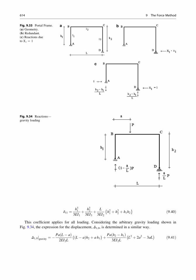
http://dx.doi.org/10.1007/978-3-319-24331-3_3

http://dx.doi.org/10.1007/978-3-319-24331-3_4

δ11 ¼ h313EI1

þ h323EI3

þ L

3EI2h21 þ h22 þ h1h2� � ð9:40Þ

This coefficient applies for all loading. Considering the arbitrary gravity loading shown in

Fig. 9.34, the expression for the displacement, Δ1,0, is determined in a similar way.

Δ1,0jgravity ¼ �Pa L� að Þ2EI2L

L� að Þh2 þ a h1f g þ Pa h2 � h1ð Þ3EI2L

L2 þ 2a2 � 3aL� � ð9:41Þ

Fig. 9.33 Portal Frame.

(a) Geometry.

(b) Redundant.(c) Reactions dueto X1 ¼ 1

Fig. 9.34 Reactions—

gravity loading


Lastly, we consider the lateral loading shown in Fig. 9.35. The displacement term due to loading is

Δ1,0jlateral ¼ � 1

EI1

Ph313

� �þ 1

EI2

Ph1L

3

h22þ h1

� �� ð9:42Þ

When h2 ¼ h1 ¼ h and I2 ¼ I1 ¼ I, these expressions simplify to

δ11 ¼ 2h3

3EIþ L

EIh2� �

Δ1,0

��gravity ¼ � Ph

2EIað Þ L� að Þ

Δ1,0

��lateral ¼ �Ph3

3EI� Ph2L

2EI

ð9:43Þ

Gravity loading:

X1

��gravity ¼ P

2

L

h

� �a=Lð Þ 1� a=Lð Þð Þ1þ 2=3ð Þ h=Lð Þ

M1

��gravity ¼ hX1

��gravity

M2

��gravity ¼ a 1� a

L

� P�M1

��gravity

Lateral loading:

X1

��lateral ¼ P

2M1

��lateral ¼ hX1

��lateral

The corresponding bending moment diagrams for these two loading cases are shown in Fig. 9.36.

Fig. 9.35 Reactions—

lateral loading


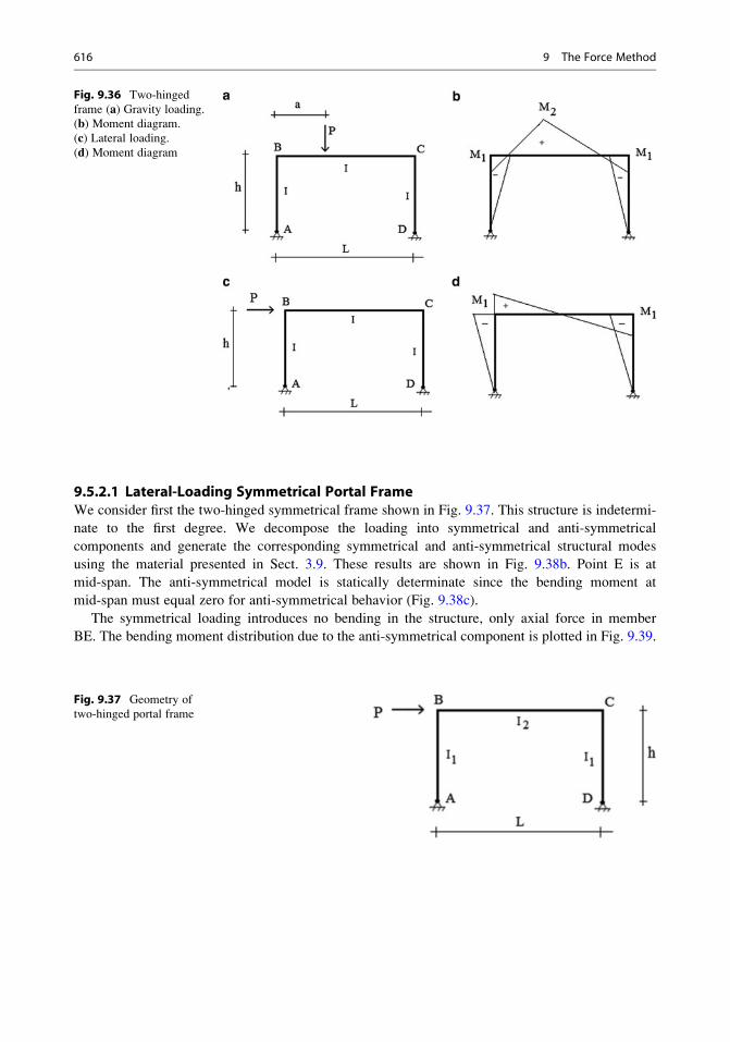
9.5.2.1 Lateral-Loading Symmetrical Portal FrameWe consider first the two-hinged symmetrical frame shown in Fig. 9.37. This structure is indetermi-

nate to the first degree. We decompose the loading into symmetrical and anti-symmetrical

components and generate the corresponding symmetrical and anti-symmetrical structural modes

using the material presented in Sect. 3.9. These results are shown in Fig. 9.38b. Point E is at

mid-span. The anti-symmetrical model is statically determinate since the bending moment at

mid-span must equal zero for anti-symmetrical behavior (Fig. 9.38c).

The symmetrical loading introduces no bending in the structure, only axial force in member

BE. The bending moment distribution due to the anti-symmetrical component is plotted in Fig. 9.39.

Fig. 9.37 Geometry of

two-hinged portal frame

Fig. 9.36 Two-hinged

frame (a) Gravity loading.

(b) Moment diagram.

(c) Lateral loading.(d) Moment diagram


http://dx.doi.org/10.1007/978-3-319-24331-3_3

Fig. 9.38 Structural models. (a) Decomposition into anti-symmetrical and symmetrical loadings. (b) Anti-symmetric

and symmetrical models. (c) Free body diagrams of anti-symmetric and symmetrical segments

Fig. 9.39 Bending

moment distribution due to

the anti-symmetrical lateral

loading


9.5.2.2 Gravity-Loading Symmetrical Portal FrameWe consider next the case of gravity loading applied to a two-hinged portal frame. Figure 9.40a

defines the loading and geometry. Again, we decompose the loading and treat separately the two

loading cases shown in Fig. 9.40b.

Geometry and Loading

The anti-symmetrical model is statically determinate. Figure 9.41 shows the model, the

corresponding free body diagram and the bending moment distribution.

The symmetrical model is statically indeterminate to one degree. We take the horizontal reaction

at the right support as the force redundant and work with the primary structure shown in Fig. 9.42.

Assuming unyielding supports, the compatibility equation has the following form

ΔD,0 þ δDDHD ¼ 0

where ΔD,0 and δDD are the horizontal displacements at D due to the applied loading and a unit value

of HD. We use the Principle of Virtual Forces specialized for only bending deformation to evaluate

these terms. The corresponding expressions are

ΔD,0 ¼ðS

M0δMdS

EI

δDD ¼ðS

δMð Þ2 dSEI

ð9:44Þ

Fig. 9.40 (a) Two-hinged frame under gravity loading. (b) Decomposition of loading into symmetrical and anti-

symmetrical components


where M0 is the moment due to the applied loading and δM is the moment due to a unit value of HD.

These moment distributions are plotted in Fig. 9.43.

Evaluating the integrals leads to:

ΔB,0 ¼ �P

2

ha

EI2L� að Þ

δBB ¼ 2h3

3EI1þ h2L

EI2

ð9:45Þ

Finally, the horizontal reaction at support D is

HD ¼ Pa L� að Þ2hL

1

1þ 2=3ð Þ rg=rc� �

" #ð9:46Þ

where

Fig. 9.42 Primary

structure for two-hinged

frame—symmetrical

loading case

Fig. 9.41 (a) Anti-symmetrical model. (b)Free body diagram—anti-

symmetrical segment.

(c) Bending moment

distribution—anti-

symmetrical loading


rc ¼ I1h

rg ¼ I2L

ð9:47Þ

are the relative stiffness factors for the column and girder members.

Combining the results for the symmetrical and anti-symmetrical loadings results in the net bending

moment distribution plotted in Fig. 9.44. The peak moments are defined by (9.48).

M1 ¼ �Pa

21� a

L

� 1

1þ 2=3ð Þ rg=rc� �

M2 ¼ þPa

2

a=Lð Þ þ 2=3ð Þ rg=rc� �

1þ 2=3ð Þ rg=rc� �

" #� Pa

21� 2a

L

� �

M3 ¼ þPa

2

a=Lð Þ þ 2=3ð Þ rg=rc� �

1þ 2=3ð Þ rg=rc� �

" #þ Pa

21� 2a

L

� � ð9:48Þ

Fig. 9.44 Final bending

moment distribution

Fig. 9.43 Bending

moment distributions—

symmetrical loading—

primary structure


Example 9.15 Two-Hinged Symmetrical Frame—Uniform Gravity Load

Given: The frame and loading defined in Fig. E9.15a.

Determine: The bending moment distribution.

Fig. E9.15a

Fig. E9.15b

Solution: We work with the primary structure shown in Fig. E9.15b. We only need to determine the

ΔD,0 term corresponding to the uniform loading since the δDD term is independent of the applied

loading. The solution for HD is

HD ¼ wL2

12h

1

1þ 2=3ð Þ rg=rc� �

where

rg ¼ I2L

rc ¼ I1h

Figure E9.15c shows the bending moment distribution. The peak values are

M1 ¼ wL2

12

1

1þ 2=3ð Þ rg=rc� �

M2 ¼ wL2

81� 2

3

1

1þ 2=3ð Þ rg=rc� �

" #


When members AB and CD are very stiff, rc ! 1 and HD ! wL2/12h. In this case, the moment

at B approaches wL2/12 which is the fixed end moment for member BC.

Fig. E9.15c Bending moment distribution

9.5.2.3 Symmetrical Portal Frames with Fixed SupportsWe consider the symmetrical frame shown in Fig. 9.45. Because the structure is symmetrical, we

consider the loading to consist of symmetrical and anti-symmetrical components. The structure is

indeterminate to the second degree for symmetrical loading and to the first degree for anti-

symmetrical loading (there is zero moment at mid-span which is equivalent to a hinge at that

point). Figure 9.45b defines the structures corresponding to these two loading cases.

Fig. 9.45 (a) Geometry.

(b) Decomposition into

symmetrical and anti-

symmetrical loadings


Evaluating the various displacement terms for the anti-symmetrical loading, one obtains:

ΔE,0 ¼ �PLh2

8EI1

δEE ¼ L3

24EI2þ L2h

4EI1

VE ¼ �ΔE,0

δEE¼ Ph

2L

� �1

1þ 1=6ð Þ L=I2ð Þ I1=hð Þð ÞThe moment diagrams are plotted in Fig. 9.46. The peak values are

M* ¼ �Ph

4

1

1þ 1=6ð Þ rc=rg� �

M** ¼ �Ph

2�1þ 1

2

1

1þ 1=6ð Þ rc=rg� ��

" #

rc ¼ I1h

rg ¼ I2L

ð9:49Þ

There are inflection points located in the columns at y* units up from the base where

y* ¼ h 1� 1

2

1

1þ 1=6ð Þ rc=rg� �

" #ð9:50Þ

When the girder is very stiff relative to the column, rc/rg ! 0 and y* ! h/2. A reasonable

approximation for y* for typical column and girder properties is �0.6 h.

Figure 9.47 shows the corresponding bending moment distribution for the two-hinged portal

frame. We note that the peak positive moment is reduced approximately 50 % when the supports

are fixed.

We consider next the case where the girder is uniformly loaded. We skip the intermediate details

and just list the end moments for member AB and the moment at mid-span (Fig. 9.48).

Fig. 9.46 Bending

moment distribution—

anti-symmetric loading


MBA ¼ �wL2

12

1

1þ 1=2ð Þ rg=rc� �

MAB ¼ 1

2MBA

ME ¼ wL2

81� 2

3

1

1þ 1=2ð Þ rg=rc� �

" # ð9:51Þ

The bending moment distribution is plotted in Fig. 9.49. The solution for the two-hinged case is

shown in Fig. 9.50. These results show that the bending moment distribution is relatively insensitive

to end fixity of the base.

M2 ¼ ME

1� 2=3

1þ 2=3 rg=rc� �

1� 2=3

1þ 1=2 rg=rc� � ¼

wL2

81� 2=3ð Þ

1þ 2=3 rg=rc� �

!

M1 ¼ MBA

1þ 1=2 rg=rc� �

1þ 2=3 rg=rc� � ¼ �wL2

12

1

1þ 2=3 rg=rc� �

! ð9:52Þ

Fig. 9.47 Moment

distribution for two-hinged

frame

Fig. 9.48 (a) Portal frame

with fixed supports under

gravity loading. (b)Moment at mid-span


9.5.3 Pitched Roof Frames

We consider next a class of portal frames where the roof is pitched, as shown in Fig. 9.51a. We choose

to work with the primary structure defined in Fig. 9.51b.

We suppose the structure is subjected to a uniform load per horizontal projection on members BC

and CD. The bending moment distribution in the primary structure due to the applied loading, M0, is

parabolic with a peak value at C (Fig. 9.52). Taking HE ¼ 1 leads to the bending moment distribution

shown in Fig. 9.53. It is composed of linear segments.

Assuming the supports are unyielding, the flexibility coefficients are

ΔE,0 ¼ � wL3

12 cos θh1 þ 5

8h2

� �1

EI2

δEE ¼ 2

3

h31EI1

þ L

EI2 cos θh21 þ h1h2 þ h22

3

� � ð9:53Þ

We define the relative stiffness factors as

r1 ¼ I1h1

r2* ¼ I2

L*ð9:54Þ

where L* is the length of the inclined roof members BC and CD.

Fig. 9.50 Bending



hinged supports

Fig. 9.49 Bending



fixed supports


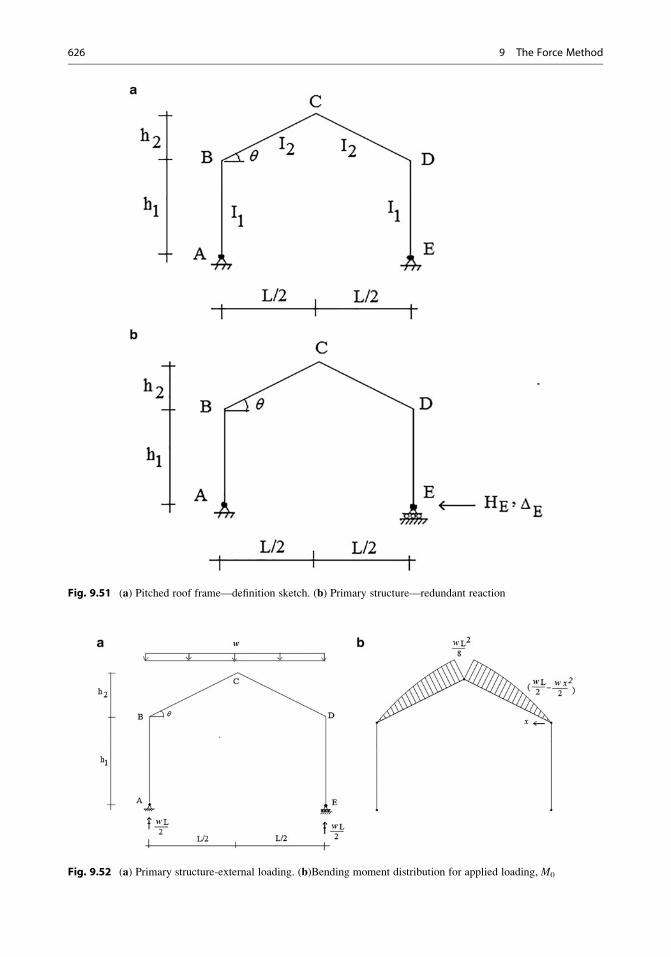
Fig. 9.52 (a) Primary structure-external loading. (b)Bending moment distribution for applied loading, M0

Fig. 9.51 (a) Pitched roof frame—definition sketch. (b) Primary structure—redundant reaction


L* ¼ L

2 cos θð9:55Þ

Using this notation, the expression for the horizontal reaction at E takes the form

HE ¼ wL2

12h1

1þ 5=8ð Þ h2=h1ð Þ1=3ð Þ r*2=r1

� �þ 1þ h2=h1ð Þ þ 1=3ð Þ h2=h1ð Þ2 ð9:56Þ

The total bending moment distribution is plotted in Fig. 9.54. Equation (9.57) contains the

expressions for the peak values.

M1 ¼ �wL2

12a1

M2 ¼ þwL2

8a2

ð9:57Þ

where

a1 ¼ 1þ 5=8ð Þ h2=h1ð Þ1=3ð Þ r2*=r1ð Þ þ 1þ h2=h1ð Þ þ 1=3ð Þ h2=h1ð Þ2

a2 ¼ 1� 2

31þ h2

h1

� �a1

ð9:58Þ

Fig. 9.54 Distribution of

total bending moments

Fig. 9.53 (a) Primary structure-unit load. (b)Bending moment distribution for HE ¼ 1


These values depend on the ratio of heights h2/h1 and relative stiffness, r2*/r1. One sets h2 ¼ 0 and

r2* ¼ 2r2 to obtain the corresponding two-hinged portal frame solution. For convenience, we list here

the relevant solution for the three-hinge case, with the notation modified to be consistent with the

notation used in this section. The corresponding moment distributions are shown in Fig. 9.55.

The peak negative and positive moments are

M1 ¼ wL2

8

h1h1 þ h2ð Þ

M2 ¼ wL2

8

1

4� 1

2

h1h1 þ h2

þ 1

4

h1h1 þ h2

� �2( ) ð9:59Þ

In order to compare the solutions, we assume r2* ¼ r1, and h2 ¼ h1 in the definition equations for

the peak moments. The resulting peak values are

Three-hinge case (9.59):

M1 ¼ �wL2

8

1

2

� �

M2 ¼ þwL2

8

1

16

� �

Two-hinge case (9.57):

M1 ¼ �wL2

8

13

32

� �¼ �wL2

80:406ð Þ

M2 ¼ þwL2

8

3

16

� �

We see that the peak negative moment is reduced by approximately 20 % when the structure is

reduced to a two-hinged frame. However, the positive moment is increased by a factor of 3.

Fig. 9.55 Three-hinge solution. (a) Loading. (b) Bending moment distribution


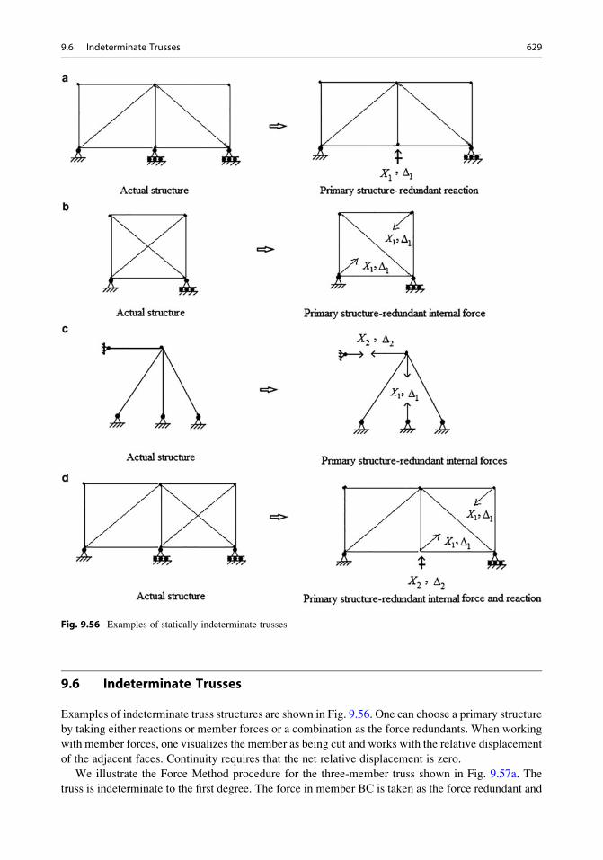
9.6 Indeterminate Trusses

Examples of indeterminate truss structures are shown in Fig. 9.56. One can choose a primary structure

by taking either reactions or member forces or a combination as the force redundants. When working

with member forces, one visualizes the member as being cut and works with the relative displacement

of the adjacent faces. Continuity requires that the net relative displacement is zero.

We illustrate the Force Method procedure for the three-member truss shown in Fig. 9.57a. The

truss is indeterminate to the first degree. The force in member BC is taken as the force redundant and

Fig. 9.56 Examples of statically indeterminate trusses

9.6 Indeterminate Trusses 629

Δ1 is the relative displacement together at the end sections. Two deflection computations are required,

one due to the external loads and the other due to X1 ¼ 1. We use the Principle of Virtual Forces

discussed in Sect. 2.3.4 for these computations. Results are summarized below.

Displacement due to external loads:

Δ1,0 ¼X F0L

AE

� �δF

¼ � 1

2 sin θ

Py

2 sin θþ Px

2 cos θ

� �L1A1E

þ � 1

2 sin θ

� �Py

2 sin θ� Px

2 cos θ

� �L1A1E

¼ � Py

2 sin 2θ

L1A1E

Displacement due to X1 ¼ 1:

δ11 ¼X

δFð Þ2 L

AE

¼ 1

4 sin 2θ

L1A1E

þ L1 sin θ

A2Eþ 1

4 sin 2θ

L1A1E

¼ 1

2 sin 2θ

L1A1E

þ L1 sin θ

A2E

Enforcing compatibility (9.3) leads to

Δ1,0 þ δ11X1 ¼ 0

Fig. 9.57 (a) Three-member truss. (b) Primary structure—redundant internal force. (c) F0. (d) δF(X1 ¼ 1)


http://dx.doi.org/10.1007/978-3-319-24331-3_2

FBC ¼ X1 ¼ �Δ1,0

δ11¼ Py=2 sin

2θ� �

L1=A1Eð Þ1=2 sin 2θð Þ L1=A1Eð Þ þ L1 sin θ=A2Eð Þ

¼ Py

A2= sin θð ÞA2= sin θð Þ þ 2A1 sin 2θ

ð9:60Þ

Lastly, the remaining forces are determined by superimposing the individual solutions.

F ¼ F0 þ δFX1

FAB ¼ Px

2 cos θþ Py

A1 sin θ

A2= sin θð Þ þ 2A1 sin 2θ

� �

FDB ¼ � Px

2 cos θþ Py

A1 sin θ

A2= sin θð Þ þ 2A1 sin 2θ

� � ð9:61Þ

As expected for indeterminate structures, the internal force distribution depends on the relative

stiffness of the members. When A2 is very large in comparison to A1, Py is essentially carried by

member BC. Conversely, if A2 is small in comparison to A1, member BC carries essentially none

of Py.

Example 9.16

Given: The indeterminate truss shown in Fig. E9.16a. Assume AE is constant, A ¼ 2 in.2, and

E ¼ 29,000 ksi.

Fig. E9.16a

Determine: The member forces.


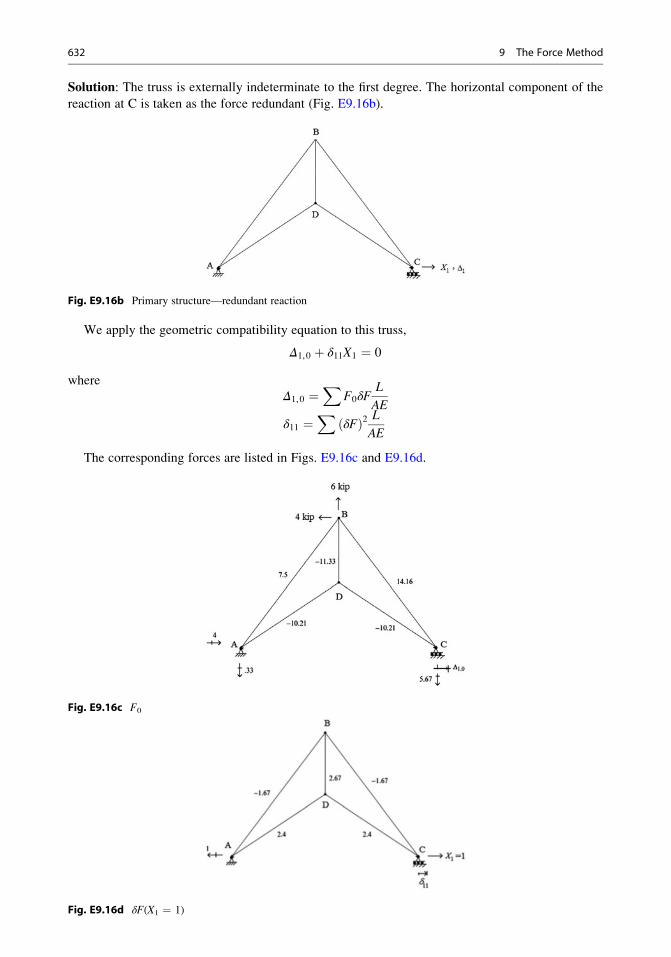
Solution: The truss is externally indeterminate to the first degree. The horizontal component of the

reaction at C is taken as the force redundant (Fig. E9.16b).

Fig. E9.16b Primary structure—redundant reaction

We apply the geometric compatibility equation to this truss,

Δ1,0 þ δ11X1 ¼ 0

where

Δ1,0 ¼X

F0δFL

AE

δ11 ¼X

δFð Þ2 L

AE

The corresponding forces are listed in Figs. E9.16c and E9.16d.

Fig. E9.16c F0

Fig. E9.16d δF(X1 ¼ 1)


Member L (in.) A (in.2)

L

A F0 δF

2(dF )L

AE 0

LF dF

AEAB 300 2 150 7.5 �1.67 418.3/E �1878.7/E

BC 300 2 150 14.16 �1.67 418.3/E �3547/E

CD 216.3 2 108.2 �10.21 2.4 625.1/E 2656/E

DA 216.3 2 108.2 �10.21 2.4 625.1/E 2656/E

BD 120 2 60 �11.33 2.67 422.7/E �1815/E

Σ 2509.5/E �12,552.7/E

Inserting this data in the compatibility equation leads to

X1 ¼ �Δ1,0

δ11¼ 12552:7

2509:5¼ 5

Then, the forces are determined by superimposing the individual solutions

F ¼ F0 þ δFX1

The final member forces and the reactions are listed below:

Member F0 δFX1 F

AB 7.5 �8.35 �0.85

BC 14.16 �8.35 5.81

CD �10.21 12.0 1.8

DA �10.21 12.0 1.8

BD �11.33 13.35 2

Rax 4.0 �5.0 �1.0

Ray �0.33 0 �0.33

Rex 0.0 +5.0 +5.0

Rey �5.67 0 �5.67


Example 9.17

Given: The indeterminate truss shown in Fig. E9.17a.

Determine: The member forces. Assume AE is constant, A ¼ 200 mm2, and E ¼ 200 GPa.

Fig. E9.17a

Solution: The truss is internally indeterminate to the first degree. The force in member BD is taken as

the force redundant (Fig. E9.17b).

Fig. E9.17b Primary structure—internal force redundant

We apply the geometric compatibility equation to this truss,

Δ1,0 þ δ11X1 ¼ 0

where

Δ1,0 ¼X

F0δFL

AE

δ11 ¼X

δFð Þ2 L

AE


The corresponding forces are listed in Figs. E9.17c and E9.17d.

Fig. E9.17c F0

Fig. E9.17d δF(X1 ¼ 1)

Member L (mm) A (mm2)

L

A F0 δF (δF)2(L/AE) F0δF(L/AE)

AB 4000 200 20 �50 �0.8 12.8 800

BC 3000 200 15 0 �0.6 5.4 0

CD 4000 200 20 �40 �0.8 12.8 640

DA 3000 200 15 0 �0.6 5.4 0

BD 5000 200 25 0 1 25 0

AC 5000 200 25 50 1 25 1250

Σ 86.4/E 2690/E

Enforcing comparability leads to

X1 ¼ FBD ¼ �Δ1,0

δ11¼ �2690

86:4¼ �31:13

∴FBD ¼ 31:13kN compression


Then, the forces are determined by superimposing the individual solutions.

F ¼ F0 þ δFX1

The final member forces and the reactions are listed below.

Member F0 δFX1 F

AB �50 24.9 �25.1

BC 0 18.68 18.68

CD �40 24.9 �15.1

DA 0 18.68 18.68

BD 0 �31.13 �31.13

AC 50 �31.13 18.87

RAx �30 0 �30

RAy 10 0 10

RDy 40 0 40

9.7 Summary

9.7.1 Objectives

• The primary objective of this chapter is to present the force method, a procedure for analyzing

statically indeterminate structures that work with force quantities as the unknown variables.

• Another objective is to use the force method to develop analytical solutions which are useful for

identifying the key parameters that control the response and for conducting parameter sensitivity

studies.


9.7.2 Key Factors and Concepts

• The force method is restricted to linear elastic behavior.

• The first step is to reduce the structure to a statically determinate structure by either removing a

sufficient number of redundant restraints or inserting force releases at internal points. The resulting

determinate structure is called the primary structure.

• Next one applies the external loading to the primary structure and determines the resulting

displacements at the points where the restraints were removed.

• For each redundant force, the displacements produced by a unit force acting on the primary

structure are evaluated.

• Lastly, the redundant forces are scaled such that the total displacement at each constraint point is

equal to the actual displacement. This requirement is expressed as

Δ��actual ¼ Δ

��loading þ

Xredundant forces

δunit forceð ÞX

where the various terms are displacements at the constraint points. One establishes a separate

equation for each constraint point. Note that all calculations are carried out on the primary structure.

9.8 Problems

Problem 9.1 Determine the vertical reaction at B. Take E ¼ 29,000 ksi and I ¼ 200 in.4

Problem 9.2 Determine the vertical reaction at B. Take E ¼ 200 GPa and I ¼ 80(10)6 mm4.

9.8 Problems 637

Problem 9.3 Determine the force in spring CD.

kv ¼ 60 kip/in.

E ¼ 29,000 ksi

I ¼ 200 in.4

Problem 9.4 Given the following properties and loadings, determine the reactions.

P ¼ 40 kN

w ¼ 20 kN/m

L ¼ 10 m

E ¼ 200 GPa

I ¼ 170(10)6 mm4

kv ¼ 40 kN/mm

δ ¼ 20 mm


Problem 9.5 Use the force method to determine the reaction at B caused by:

1. The distributed load shown

2. The support settlement at B

9.8 Problems 639

I ¼ 400 in:4

L ¼ 54ft

w ¼ 2:1kip=ftδB ¼ 1:2 in: #E ¼ 29, 000ksi

Problem 9.6 Use the force method to determine the forces in the cables. Assume beam is rigid.

AC ¼ 1200 mm2, L ¼ 9 m, P ¼ 40 kN, and E ¼ 200 GPa.

Problem 9.7 Consider the parabolic arch shown below. Assume the arch is non-shallow, i.e., h/L is

order of (1/2).


y ¼ 4hx

L� x

L

� 2� �

I ¼ Iocos θ

(a) Determine the horizontal reaction at B due to the concentrated load.

(b) Utilize the results of part (a) to obtain an analytical expression for the horizontal reaction due to

a distributed loading, w(x).

(c) Specialize (b) for a uniform loading, w(x) ¼ w0.

(d) Suppose the horizontal support at B is replaced by a member extending from A to B. Repeat part

(a).

Problem 9.8 Consider the semicircular arch shown below. Determine the distribution of the axial

and shear forces and the bending moment. The cross-section properties are constant.

Problem 9.9

9.8 Problems 641

Use a computer software system to determine the bending moment distribution and deflected

shape produced by the following loadings.

TakeA ¼ 20, 000mm2, I ¼ 400 10ð Þ6mm4 and E ¼ 200GPa

Problem 9.10A ¼ 30 in:2 I ¼ 1000 in4 E ¼ 29, 000ksi

Use a computer software system to determine the maximum bending moment and the axial force in

member ABC. Consider the following values for the area of the tension rod AC: 4, 8, and 16 in.2

Problem 9.11

A ¼ 40 in:2 I ¼ 1200 in:4 E ¼ 29, 000ksi

Use a computer software system to compare the bending moment distributions generated by the

following loadings:


Problem 9.12 Determine the horizontal reaction at support D.

9.8 Problems 643

Problem 9.13 Determine the peak positive and negative moments as a function of h. Consider

h ¼ 2, 4, 6 m.

Problem 9.14 Determine the peak positive and negative moments as a function of h. Considerh ¼ 10, 20, 30 ft.

Problem 9.15 Using a computer software system, determine the bending moment distribution and

deflected shape due to the loading shown.


Take I1 ¼ 1000 in.4, I2 ¼ 2000 in.4, E ¼ 29,000 ksi, and A ¼ 20 in.2 all members.

Problem 9.16 Compare the bending moment distributions and the vertical displacement at B for the

structures defined below. Take E ¼ 200 GPa, I ¼ 400(10)6 mm4, A ¼ 100,000 mm2, and

Ac ¼ 1200, 2400, 4800 mm2. Use a computer software system.

9.8 Problems 645

Problem 9.17 Is there any difference in behavior for the structures shown below? Answer the

question without resorting to calculations.

Problem 9.18 Determine the reactions and the member forces for the truss shown. Assume the

vertical reaction at d as the force redundant.

E ¼ 200 GPa

A ¼ 660 mm2 all members

α ¼ 12 � 10–6/�CΔT ¼ 10 �C


Problem 9.19 Determine the forces in the members. E ¼ 29,000 ksi and A ¼ 1 in.2 all members.

Problem 9.20 Determine the member forces of the truss shown. Assume the horizontal reaction at

c as the force redundant.

A1 ¼ A2 ¼ A3 ¼ A4 ¼ 10 in.2

A5 ¼ 5 in.2

α ¼ 6.5 � 10–6/�FΔT ¼ 60 F

E ¼ 29,000 ksi

9.8 Problems 647

Problem 9.21 Determine the member forces for the truss shown. Assume A ¼ 1000 mm2 and

E ¼ 200 GPa for all the members. Take the force in member ac and the reaction at support f as theforce redundants.

Reference

1. Tauchert TR. Energy principles in structural mechanics. New York: McGraw-Hill; 1974.


Documents

The Force Method 9...The Force Method 9 Abstract Up to this point, we have focused on the analysis of statically determinate structures because the analysis process is fairly straightforward;