The Forecasting Performances of Volatility Models in ... 3_2_4.pdf · The Forecasting Performances of Volatility Models in Emerging ... SHCOMP, SENSEX, KOSPI, FBMKLCI, PCOMP, CSEALL,

Journal of Applied Finance & Banking, vol. 3, no. 2, 2013, 49-73

ISSN: 1792-6580 (print version), 1792-6599 (online)

Scienpress Ltd, 2013

The Forecasting Performances of Volatility Models in

Emerging Stock Markets: Is a Generalization Really

Possible?

Zeynep Iltuzer1 and Oktay Tas2

Abstract

In almost all stages of forecasting volatility, certain subjective decisions need to be made.

Despite of an enormous literature in the area, these subjectivities are hindrances to

reaching an overall conclusion on the performances of the models. In order to find out

outperforming model in general not just in the contexts of studies, volatility models

should be evaluated in many markets with the same methodology consisting both simple

and complex models at different forecast horizon. With this motivation, the purpose of

the paper is to search for the possibility of the generalization that one of the competing

model outperforms no matter what the market is by analyzing 19 emerging stock market

volatilities at 8 different forecast horizons with models grouped into three main categories:

Simple models (Random Walk, Historical Mean, Moving Average, EWMA), GARCH

family models (GARCH, GRJ-GARCH, GARCH, APARCH, NAGARCH, FIGARCH)

and Stochastic Volatility model. The evaluation of the forecasts based on the recent

developments in statistics, i.e. Reality Check (RC), Superior Predictive Ability (SPA) and

Model Confidence Set (MCS), not only the rank of the error statistics. The scope and the

methodology of the study enable us to reach a general conclusion on model performances

and their over prediction and under prediction tendencies.

JEL classification numbers: G17, G15, C22

Keywords: Emerging Markets, GARCH, Stochastic Volatility, MCS, SPA, RC

1Istanbul Technical University, Management Faculty, Management Engineering Department.

e-mail: [email protected] 2Istanbul Technical University, Management Faculty, Management Engineering Department,

e-mail: [email protected]

Article Info: Received : September 21, 2012. Revised : October 11, 2012.

Published online : March 1, 2013

mailto:[email protected]

mailto:[email protected]

50 Zeynep Iltuzer and Oktay Tas

1 Introduction

Varied subjective decisions in different dimensions need to be made during the process of

forecasting volatility and the comparison of forecasts. [1] is a very good source to see

these subjectivities and other issues in forecasting volatility and to gain insight what kind

of questions arise when forecasting volatility in financial markets such as which approach

will be used for the proxy of observed volatility, which competing models will be

included, what the forecast horizons will be, which error statistics will be used for the

comparison, and how error statics will be evaluated to reach the conclusion on the

performance of the models. The decisions based on these questions naturally affect the

results of researches, which eventually is a handicap in the area of forecasting volatility to

compare and evaluate the results of the previous studies. As it is pointed out by [2], even

for a certain stock market, different conclusions are drawn due to the different

observations and forecasting methodology. Hence, the performance of volatility models is

evaluated in myriad number of studies; the results of the studies are relevant only in their

own context. To find out whether there really is a model that performs better than the

alternatives, they need to be evaluated all together with the same methodology in order to

eliminate the effect of these subjective decisions on the forecasting performances. To be

able to accomplish this, the models included in the analysis needs to be as comprehensive

as possible, the number of markets needs to be as large as possible and the comparison of

the error statistics should depend on some statistical analysis not just the rank of the error

statistics. The rest of this section briefly explains these subjectivities in forecasting

volatility in order to see the reason behind the motivation to perform such an analysis.

Firstly, there are two different approaches to measure volatility in the literature: variance

and standard deviation. [3], [4], [5] and [6] used variance as a volatility measure while [7],

[8] preferred standard deviation. Secondly, the researcher has to decide how to measure

observed volatility since it is a latent variable. General approaches are daily squared

returns [9], [10], mean adjusted daily squared returns [11], [12], daily squared return

adjusted for serial correlation [4], [13], the absolute change in returns [14], [15]3. The

existence of different approaches is mainly based on the question of whether the returns

are adjusted for mean (conditional or constant) or not. The advocates of the use of squared

returns adjusted for mean and serial dependence put forward that empirically proved high

autocorrelation in the return should be controlled while the opponents claim that the

statistical properties of the sample mean make it very inaccurate estimate of true mean,

therefore taking deviations around zero instead of sample mean increases the forecast

accuracy.

Another difference in studies in the area of forecasting volatility is that how the sample is

used for parameter estimation and forecasts. One of the approaches is to apply a rolling

scheme to estimate parameters of the models as in [5], [16] etc. The other approach,

which is more commonly preferred, is that the division of data as in-sample and

out-of-sample just once as in [17], [2]. Since in-sample data, therefore, the parameter

estimates, is updated for every forecast in the rolling scheme approach, this approach may

provide a better reflection of the structural changes in the economy to the parameters of

the model and may prevent biases which depend on fixing in-sample for every forecast on

3Since there is an enourmous literature on forecasting volatility, it is not just practical to list every

refrence to make the point. Only a few of them have been given here.

The Forecasting Performances of Volatility Models 51

the model performances. From this point of view, the rolling scheme approach is

preferred in the paper.

The comparison of model performances is quite important in the process of evaluation of

the models performances. Although this stage is as important as forecasting; the

comparison of error statistics has been limited to the evaluation of the rank of some error

statistics, which are the subjective choice of researchers, so far. The conclusions are

basically drawn from the rank obtained by the error statistics. However, error statistics of

the competing models are most of the time so close that the question that the

performances of the models are really distinguished from one another arises. The recent

developments in econometrics, namely Reality Check (RC), Superior Predictive Ability

(SPA) and Model Confidence Set (MCS), provide a solution to this problem. These

procedures help the evaluation of the error statistics in a way that researches can be sure

about the statistical significance of the ranks implied by the error statics, which in fact put

the comparison in a more sound ground. The choice of error statistic is another issue for

the comparisons. As it is stated in [18], it directly affects the evaluation of model

performances. Most commonly used error statistics in the area of forecasting volatility are

those that have symmetric property. Later, asymmetric error statistics has started to be

used in order to address different exposure of risks coming from the positions (long/short)

of investors in markets. In the paper, both symmetric and asymmetric error statistics have

been included in the evaluation process of models.

As for the forecast horizon, the relevant forecast horizon varies by the purpose of the

agents. Short forecast horizons are relevant for trading purposes and VaR estimations of

financial institutions. For derivative markets, longer horizons are also relevant. Besides

this, while a certain model performs very well in a specific forecast horizon, it may not be

the same for the other horizons. Therefore, the evaluation of model performances in

different horizons would provide some insight about the forecasting ability of the models

in different horizons. Since the purpose of the paper is to evaluate the model

performances in a general context, the results are evaluated for eight different forecast

horizons varying between 1-day and 240-day.

Finally, which models should be included in the analysis is also critical since the

performances are relatively evaluated. Therefore, the comprehensiveness of an analysis in

terms of models that are included increases the generalizability of the results. With this

perspective, the study covers Random Walk, Historical Mean, Moving Average, and

EWMA as simple nonparametric models and GARCH family models and Stochastic

volatility models as parametric models. Lately, the researches that apply and/or develop

Stochastic Volatility model is more popular and mostly focus on the parameter estimation

methods, however, GARCH family models are still dominant in the literature. Many

GARCH models are developed by the different researchers with different approaches in

order to incorporate the empirically proved patterns in volatility in the stock market

returns, i.e. leverage effect, nonlinearity, long-memory. Therefore the inclusion of all

developed GARCH family models is simply not practical. To address this issue, a

representative set of GARCH family models are formed in order to cover the models

addressing at least one of the above mentioned volatility patterns.

In summary, all of the points mentioned above complicate any attempt to compare and

generalize the results in volatility forecasting literature. This paper aims to complement

the literature in two ways. Firstly, to the best of our knowledge, this is the most

comprehensive study for emerging stock markets in terms of the number of countries (i.e.


19 stock exchanges), the variety of the forecast horizons (short-, mid- and long-term) and

the number of models (11 models). The comprehensiveness in different dimensions

provides one to draw general conclusions in forecasting performances of the models for

emerging stock markets. Secondly, this study is distinguished from the others by its

comparison methodology.

2 Volatility Models and Forecasting Methodology

This section briefly introduces the data, volatility models and the methodology. Argentina,

Brazil, Chile, Mexico, Peru, Venezuela, Czech Republic, Hungary, Poland, Russia,

Turkey, China, India, Korea, Malaysia, Philippines, Srilanka, Taiwan, Thailand emerging

stock market indices have been chosen based on SP/IFC classification and daily data are

obtained from Bloomberg databases4.

Daily observed volatilities are estimated as mean adjusted daily squared return, i.e.

and since the data is in daily frequency, h-day observed volatilities are

estimated as the sum of the daily volatilities for the relevant period, which is

where i = 1, 1 + h, 1 + 2h, ... and is the logarithmic return, μ is

the sample mean, and h = 1, 5, 10, 20, 60, 120, 240 days are the forecast horizons. The

data is divided into two parts since the focus is to compare the out-of-sample forecasts.

The rolling scheme in which the sample size and forward shifting step was fixed at

w=2000 and s=20 respectively is applied for the estimations. Below is the brief

explanation of the models and the forecasting procedure:

Random Walk (RW): The best forecast of the tomorrow volatility is today volatility:

(1)

where t = w,w + s,w + 2s, ... is the volatility forecast,

is the observed volatility,

w is the sample size, s the forward shifting step in the rolling scheme.

Historical Mean (HM): This is basically the mean of all observations before the relevant

forecast is performed. That is, the sample size grows as additional observations are added.

(2)

where t = w,w + s,w + 2s, ...

Moving Average (MA): According to HM, all past observation is used for the forecast.

However, MA only takes into account past n observations, which is a subjective choice.

MA can be considered as a recent historical mean of the variable. In the paper n is chosen

as 240, which can be considered as one-year historical mean:

(3)

where t = w,w + s,w + 2s, ... and k = w - n + 1,w - n + s + 1,w - n + 2s + 1, ....

4The Bloomberg tickers are respectively MERVAL, IBOV, IPSA, MEXBOL, IGBVL, IBVC, PX,

BUX, WIG20, RTSI, XU100, SHCOMP, SENSEX, KOSPI, FBMKLCI, PCOMP, CSEALL,

TWSE, SET. The data period for all indices is the same and between 2nd January 1995 and 23th

April 2010 except Russia for which it starts on 2nd April 1995.


Exponentially Weighted Moving Average (EWMA): As opposed to MA, EWMA gives

exponentially decreasing weights to past observations as past observations gets older. The

intuition behind incorporation of decay in weights is that recent observations have much

more importance in forecasting future volatility than older observations.

(4)

where t = w,w + s,w + 2s, ... , n= 240 and λ is the smoothing constant and estimated by

minimizing the sum of in-sample squared errors in the study.

h-day volatility forecasts of the above nonparametric models are estimated by simple

scaling rule ,which is .

The GARCH family models: It is not wrong to say that the current interest in volatility

modeling and forecasting started with the seminal papers [19] and [20] in which GARCH

and ARCH models were proposed respectively. After these seminal papers, variety of

versions taking into account different characteristics of financial time series such as

leverage effect, long memory, nonlinearity have been developed from GARCH modeling

perspective. Therefore, the literature on conditional volatility models is enormous.

Although the entire GARCH model universe is not included in the analysis, selected

models, namely GARCH, GJR-GARCH, EGARCH, APARCH, NAGARCH and

FIGARCH, can be considered as a representative set of GARCH family models since the

model set includes those focusing on different patterns in volatility such as asymmetry,

nonlinearity and long memory.

Let define as the return process of the stock market.

, (5)

GARCH(1,1) model [19]:

(6)

GJR-GARCH(1,1) model [21]:

(7)

where if , otherwise.

EGARCH(1,1) model [22]:

(8)

Asymmetric Power ARCH - APARCH(1,1) model [23]:

(9)

Nonlinear Asymmetric GARCH - NAGARCH(1,1) model [24]:

(10)

Fractionally Integrated GARCH -FIGARCH(1,d,1) model [25]5:

5For the parameter estimation of FIGARCH, NAGARCH and APARCH models Prof. Kevin

Sheppard’s matlab codes, which are provided in his website


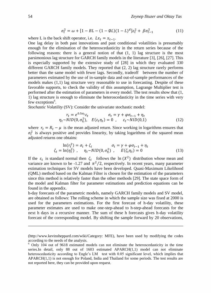
(11)

where L is the back shift operator, i.e. .

One lag delay in both past innovations and past conditional volatilities is presumably

enough for the elimination of the heteroscedasticity in the return series because of the

following reasons: there is a general notion of that (1, 1) lag structure is the most

parsimonious lag structure for GARCH family models in the literature [3], [26], [27]. This

is especially supported by the extensive study of [28] in which they evaluated 330

different GARCH family models. They reported that (2, 2) lag structure rarely performs

better than the same model with fewer lags. Secondly, tradeoff between the number of

parameters estimated by the use of in-sample data and out-of-sample performances of the

models makes (1,1) lag structure very reasonable to use in forecasting. Despite of these

favorable supports, to check the validity of this assumption, Lagrange Multiplier test is

performed after the estimation of parameters in every model. The test results show that (1,

1) lag structure is enough to eliminate the heteroscedasticity in the time series with very

few exceptions6.

Stochastic Volatility (SV): Consider the univariate stochastic model:

, , (12)

where is the mean adjusted return. Since working in logarithms ensures that

is always positive and provides linearity, by taking logarithms of the squared mean

adjusted returns one obtains:

,

, (13)

If the is standard normal then follows the distribution whose mean and

variance are known to be -1.27 and , respectively. In recent years, many parameter

estimation techniques for SV models have been developed. Quasi-Maximum Likelihood

(QML) method based on the Kalman Filter is chosen for the estimation of the parameters

since this method is relatively faster than the other methods [29]. The state space form of

the model and Kalman filter for parameter estimations and prediction equations can be

found in the appendix.

h-day forecasts of the parametric models, namely GARCH family models and SV model,

are obtained as follows: The rolling scheme in which the sample size was fixed at 2000 is

used for the parameters estimations. For the first forecast of h-day volatility, these

parameter estimates are used to make one-step-ahead to h-step-ahead forecasts for the

next h days in a recursive manner. The sum of these h forecasts gives h-day volatility

forecast of the corresponding model. By shifting the sample forward by 20 observations,

(http://www.kevinsheppard.com/wiki/Category: MFE), have been used by modifying the codes

according to the needs of the analysis. 6 Only 104 out of 9618 estimated models can not eliminate the heteroscedasticity in the time

series.In detail, only 88 out of 1603 estimated APARCH(1,1) model can not eliminate

heteroscedasticity according to Engle’s LM test with 0.05 significant level, which implies that

APARCH(1,1) is not enough for Poland, India and Thailand for some periods. The test results are

not reported here, they can be provided upon request.

http://www.kevinsheppard.com/wiki/Category:%20MFE


the new parameter estimates are obtained. One-step-ahead to h-step-ahead forecasts for

the next h days are performed in a recursive manner with these new parameters for the

second forecast of h-day volatility. It continues in the same way until the end of the

sample.

3 Comparison Of Forecast Performances

A sound comparison of model performances is as important as performing the forecasts.

Both symmetric and asymmetric error statistics are relevant for the evaluation of the

volatility forecasts in stock markets. Asymmetry in the error statistics can be especially

important for participants of derivative market. For example, the major parameter that

determines the value of an option contract is volatility of the underlying, the investors

who take long/short position may prefer to penalize over/under predictions more heavily

to reduce to exposure to volatility modeling risk. However, it should be noted that the

symmetric error statistic are more suitable to evaluate a model overall success in terms of

fitting to observed data. Hence, performance results of the models are primarily deduced

from the symmetric error statistics, while asymmetric error statistics are used to determine

the tendencies of models in general in making over/under predictions with the purpose of

addressing the different needs of the investors. The following error statistics are used in

the study7.

Symmetric error statistics8:

(14)

Asymmetric error statistics9:

(15)

where k denotes the number of over predictions and l the number of under predictions

among the out-of-sample forecasts, which is .

(16)

where the choice of the value of the parameter a is subjective, which allows different

weights to over- and under-predictions. When , it punishes heavily the under

7Error Statistic of the models for the markets are not presented in the paper. Upon request, the file

that contains the tables can be provided. 8MSE, RMSE, MAE, MAPE stand for Mean Square Error, Root Mean Square Error, Mean

Absolute Error, Mean Absolute Percentage Error, respectively.

9MME-U, MME-O, MLAE stand for Mean Mixed Error-Under, Mean Mixed Error-Over, Mean

Logarithm of Absolute Error, respectively.


predictions. In the study .

To evaluate by just looking at the rank implied by the error statistics does not provide a

sound comparison. Fortunately, in the last decade, some important statistical techniques

have been developed to check whether the rank of the performances of the models

deduced from a certain error statistic is statistically significant or not. Reality Check (RC)

in [30] and Superior Predictive Ability (SPA) in [31] tests allow us to determine whether

the differences obtained from error statistics are significant or not. The null hypothesis of

both RC and SPA are that the models included in the analysis do not have superior

performance relative to the benchmark, while the alternative hypothesis is that at least one

of the models has superior forecasting performance relative to the benchmark. This

implies that, the performance of the model that has the best error statistic is superior to the

benchmark even though one would not tell anything about the comparison between the

best model and models other than the benchmark. During the empirical analysis, it has

seen that the best model does not always show significantly superior performance than the

benchmark according to certain error statistics, while it does according to some other

error statistics. Therefore, these tests can also be used to determine which error statistics

can really distinguish the performances of models. The difference between these two tests

is that RC is quite sensitive to the set of the models included in the analysis. That is, if the

comparison involves irrelevant or poor alternatives, then RC is not able to reject the null

hypothesis even though it is the case. When the model set comprises reasonable

alternative both RC and SPA produce quite similar results. In this study, when RC and

SPA test are performed the simplest model RW is chosen as the benchmark model. The

other technique used to distinguish the performances of the models is the Model

Confidence Set (MCS) procedure of [32]. The MCS method characterizes the entire set of

models as those that are/are not significantly outperformed by other models, on the other

hand, RC and SPA tests only provide evidence about the relative performance according

to the benchmark model. [32] illustrates the difference between RC/SPA and MCS with

analogy of the difference between confidence interval of a parameter and point estimate

of a parameter. The significance of the performance of the best model relative to the

benchmark can be determined with RC and SPA tests, however, RC and SPA tell nothing

about the case in which the performances of other models are very close to the model that

shows the best performance. At that point, The MCS helps one determine whether the

performances of other models performances are close to the best model or not by

grouping the models into two categories (sets), namely inferior and superior models sets,

by assigning probability values to each model. If p-value of a model is greater than a

subjectively determined p-value, then it is accepted as in the superior set. The critical

p-value for the study is chosen as 0.9. In the study, all of the three techniques are used for

the evaluation of the forecasting performances. First step is to determine which error

statistics give significant results by applying SPA and RC tests. At this step, the best

performing model can be confidently declared as the best performing model according to

corresponding error statistic, however, to what extent that the best performing model is

significantly superior than the other models can only be determined by the MCS

procedure, which is the second step of the evaluation process10

.

10For SPA, RC and MCS estimations, Prof. Kevin Sheppard’s matlab codes , which are provided in

his website (http://www.kevinsheppard.com/wiki/Category:MFE), have been used. SPA/RC test

results and MCS p-values can be provided upon request.

http://www.kevinsheppard.com/wiki/Category:MFE


4 Empirical Analysis and Results

In this section, out-of-sample forecasts of 11 models for short-term (1-day, 5-day, 10-day),

medium-term (20-day, 60-day and 120-day) and long-term (180-day and 240-day)

forecast horizons are performed and compared. Table 1 to Table 8 presents the results.

Since the results in the table are based on the error statistics and RC, SPA, and MCS test

results, the following points should be taken into account in order to be able understand

how conclusions are drawn from the tables. First of all, the best performing model

according to each error statistic is reported in the tables as the first input of the cells.

When the best performing model is significantly different from the benchmark based on

RC/SPA tests results, the model is superscripted by ”*” and is called ”the significant best

model”. Hence, if there is not any model superscripted by “*” in a cell than the

performances of models are not significantly different from each other according to

corresponding error statistic. This is the first step of the evaluation of the results of the

error statistic. It in fact provides one to determine which error statistic results should be

taken into account for the rest of the comparison process.

Let consider 1-day volatility forecast results for PERU in Table 1. According to MSE,

NAGARCH is the best model while EWMA is the best model according to RMSE.

However, RC/SPA test results show that MSE cannot distinguish the model performances

while RMSE does. Therefore, the best model according to MSE is not taken into account

for the rest of the analysis, and the result of RMSE, i.e. EWMA, is superscripted to show

that it will be taken into account for the rest of the comparison process. That is, only

superscripted models and corresponding error statistics are evaluated after that point. As

explained in section III, even though a model is determined as the significant best model

with the help of RC/SPA tests, this doesn’t tell anything about the difference between the

best model and the second best model, third best model and so on. The second step of the

evaluation process addresses to this issue by determining MCS set of superiors of the

significant best model if there is one. If there exists a MCS set of superiors for a

significant best model, then the models in the MCS are added to place where the

significant best model is in the table. Therefore, where the cells include more than one

model, they report the set of models whose performances are the same as that of the

significant best model, which is superscripted by *. This set of models will be

called ”MCS set of superiors” of the corresponding significant best model. If we back to

the example of PERU in Table 1, MCS set of superiors of EWMA is NAGARCH and

GRJ-GARCH. Lastly, the success of the models are evaluated based on the symmetric

error statistic, and the asymmetric error statistic are used to determine the tendency of the

models in making under/over predictions, which is considered as beneficial for those who

have preferences over under/over prediction in their decision processes.

First thing that should be noticed in Table 1 is the outperformance of SV model on 1-day

volatility forecasts. For 14 out of 19 stock markets, SV is the significant best model

according to more than one error statistics for most of the markets. For a few of these

markets, namely Argentina, Czech and China, the MCS set of superiors of SV comprises

GARCH family models, which means that SV is sharing the same performance level as

GARCH family models for 3 out of 14 markets. Even though the performance of GARCH

family models is close to that of SV for these three market SV is successful in 14 markets.

Therefore, it is not wrong to make the generalization that SV model is the best model to

forecast stock market volatility in emerging markets for 1-day volatility forecasts. On the


other hand, this outstanding success of SV is completely vanished for 5-day volatility

forecasts since it does not show the best performance even at one market as it can be seen

from Table 2. This is a quite strong indication of that the smaller the forecast horizon, the

better the performance of SV gets. For 5-day volatility forecasts, GARCH family models

have dominance over the others by outperforming in 11 out of 19 emerging markets.

EWMA is the second model by outperforming in 7 out of 19 markets. When the MCS set

of superiors of the models are examined, the MCS set of superiors of GARCH family

models includes EWMA only in 2 out of 11 markets, and the MCS set of superiors of

EWMA includes GARCH family models in 3 out of 7 markets. This implies that there is

not an important intersection in which these two models show the same out-performance

in the same markets. Over all, when MCS results are taken into account, GARCH family

models outperform in 15 markets (11 as the best model + 4 as the MCS set of

superiors of other models), while EWMA outperforms in 9 markets (7 as the best model +

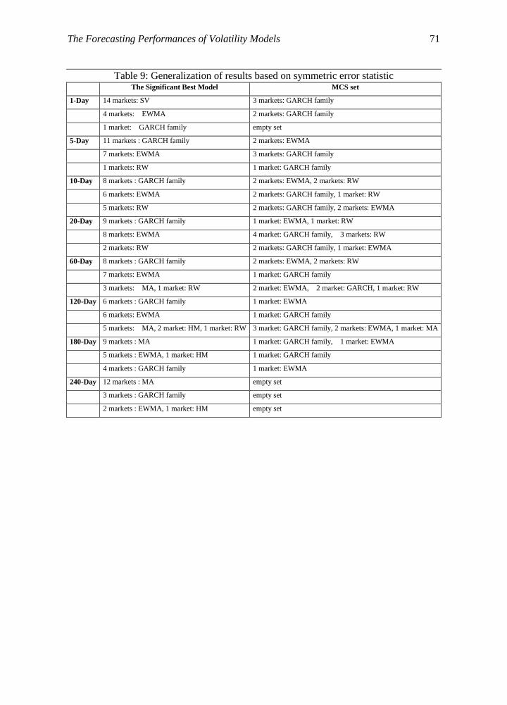
2 as the MCS set of superiors of other models). Table 9 provides quick overlook this

whole 11+4 and 7+2 summation and generalization process by reporting the number of

cases (markets) in which a certain model is the best model and the number of cases

(markets) in which the model is the MCS set of superiors of other models11

. So, GARCH

family model are considerably successful for 5-day volatility forecasts. Therefore, it

would be more reasonable to choose GARCH family models for 5-day volatility forecasts

in the case that one has to choose a volatility model without performing any forecasting

analysis. As for the results of 10-day volatility forecasts in Table 3, GARCH family

models and EWMA show outperformance in almost equal number of markets, and again

the MCS set of superiors of either one include each other in the same number of markets.

RW is another model found as the significant best model for 5 out of 19 markets for

10-day volatility forecasts. However, the MCS set of superiors of RW involves GARCH

family models and EWMA for 4 out of these 5 markets. This implies that RW just shares

the same performance level as those of EWMA and GARCH family models in those 4

markets, which eventually strengthens the generalization of outperformance of GARCH

family models and EWMA for 10-day volatility forecasts. Furthermore, if it is

remembered that EWMA is a special case of Integrated GARCH model, this is a very

strong support for the choice of GARCH family models for 10-day volatility forecasts.

For 20-day volatility forecasts, the out-performance of GARCH family models is

noteworthy in Table 4. GARCH family models are the significant best model for 9 out of

19 markets. Also, they are MCS set of superiors of both EWMA , in 4 out of 8 markets,

and RW, in 2 out of 2 markets. This implies that GARCH family models are the

significant best model for 9 markets and they show the same performance level as

EWMA and RW for additional 6 markets, that is, in total, for 15 out of 19 markets,

GARCH family models have superior performance. For both 60-day and 120-day

volatility forecasts in Table 5 and Table 6 respectively, EWMA and GARCH family

models outperform in almost equal number of markets. However, it should be noted that,

as the forecast horizon increases, the number of markets where EWMA is the best models

is getting closer to that of GARCH family models, And MA also starts to outperform in

some markets. For 60-day volatility forecasts, MA is the significant best model in 3

markets; however, it shares the same performance level as those of GARCH family

11While Table 1 to Table 8 reports the results for each horizon, Table 9 and Table 10 facilitate to

see the generalizations deduced from these tables.


models and EWMA in these markets. On the other hand, for 120-day volatility forecast,

MA is the significant best model in 5 markets, and it shares the same performance level

only in 1 out of these 5 markets as those of GARCH family models and EWMA, which is

the first sign of that how MA gets stronger as the forecast horizon increases.

For 180-day volatility forecasts, MA is the significant best model for almost half of the

markets in Table 7, while the rest of the markets are shared by GARCH family models

and EWMA. As for 240-day volatility forecasts in Table 8, MA has dominance over the

other models by outperforming 12 out of 19 markets. It is not wrong to make the

generalization that MA is the best choice to forecast stock market volatility in emerging

markets for 240-day volatility forecasts.

When the results of asymmetric error statistics are evaluated, the first striking result is

that SV model consistently under predicts, and GARCH family models over predict for

almost all forecast horizons. Table 10 provides the generalization of the over prediction

and under prediction patterns of the models for different forecast horizon. The choice of

over prediction or under prediction depends on investors’ preferences. Generally, some

investors may find it beneficial to choose models that over predict for the sake of being in

the safe side. However, it should be noted that GARCH family models over predict at the

ordinary times. It implies that investors, who use GARCH family models for prediction,

are being too cautious in ordinary times, and may not be ready enough for the high risk

periods. Therefore it is recommended that the investors should ask themselves the

question of how this over prediction (or under prediction) pattern in ordinary times affects

their positions and pricing decisions. Especially in option markets, investors can take

positions on the volatility of the underlying. For instance, investors who use

straddle/strangle are exposed to different risks inherent in forecasting of volatility of the

underlying. Let think about an investor who applies straddle strategy on an underlying

places his bids based on the volatility forecast of the underlying for the relevant horizon.

There is a possibility that he prices the options contracts higher than they should be in

case that he uses GARCH family models. Or let think that he writes straddles on a certain

underlying. In this case if he forms his volatility expectation of the underlying by the

forecast of SV model, he is exposed to risk of predicting the volatility lower than it should

be. Therefore he increases the possibility of loss in his position without having been

sufficiently compensated for the risk that he carries due to lower ask price. At that point,

there are a few things to be mentioned about the use of symmetric and asymmetric error

statistics. If a model is the best model according to both symmetric and asymmetric error

statistics, this model is what investors look for if they have preferences over under

prediction or over prediction. If a GARCH family model is the significant best model

according to both symmetric and asymmetric error statistics, it should be interpreted as

the model produces the closest prediction to the observed volatility but usually the

predictions are higher than the observed one, which is very suitable for those who apply

straddle if we back to the example above.

Beside the performance of the models, there are a few points needed to be mentioned.

First of all, as the forecast horizon increases, the significant best models uniquely

outperform in the relevant markets. That is, while more than one models share the same

performance levels for the most of the markets for 1-day volatility forecasts, as the

horizon increases difference in the model performances gets bigger, and eventually for

240-day forecast horizon, the MCS set of superiors of the significant best models are

empty sets for the all markets. Secondly, as a side result of this study, it is found that


RMSE is the only symmetric error statistic that can always distinguish the model

performances no matter what the forecast horizon is. If the scope of this study is taking

into account, the success of RMSE is so consistent that it is not wrong to say that RMSE

is the strongest symmetric error statistic in terms of the power of distinguishing

differences among the models.

The results provide a very good reference for the choice of volatility model for different

forecast horizon even though it is not the main motivation of the study. Table 11

presents the best volatility model for each emerging market at different forecast horizon.

General tendency both in academia and in practice is to use GARCH family models to

estimate and forecast volatility. This tendency is so strong that GARCH family models

are almost default choice. However, Table 11 tells that this widespread use of GARCH

family models is not that appropriate in every case. From table 11, one can find that the

simple models like EWMA and MA are the best model for many forecast horizons. The

results are not commented here country by country, the reader can make inferences easily.

However, there are a few pattern that needs to be mentioned specifically. For three

emerging markets in Europe, namely Turkey, Poland and Russia, EWMA is the best

model in most forecast horizons. Hence, for the actors in these markets, the best choices

for volatility model is EWMA not GARCH family models. Many institution use GARCH

family models to calculate their market risk as a part of their capital adequacy ratio.

However, Table 10 in which over prediction and under prediction tendencies of the

models in general are reported implies that GARCH family models usually overpredict,

which means that these institutions may have unnecessarily low capital adequacy ratios.

On the other hand, GARCH family models are the best volatility models at all forecast

horizon for the stock market in Czech Republic. Another pattern which is quite strong

fort the stock market in Thailand is that FIGARH model is quite successful at almost all

forecast horizon.

5 Conclusion

In the paper, the forecast evaluations of the volatilities of the 19 emerging stock market

indices for forecast horizons from 1 day to 240 days are performed with the purpose of

examining whether there really is a certain model superior to the alternatives for the

majority of the emerging markets. The most general results can be listed as follows: First

of all, SV is the best performing model for 1-day volatility forecasts for majority of the

emerging market. For 10-day, 20-day, 60-day and 120-day volatility forecasts, GARCH

family models and EWMA show superior performance in almost equal number of

countries, and, EWMA outnumbers GARCH family models as the forecast horizon

increases. For 240-day volatility forecasts, MA outperforms for most of the countries.

That is, as the forecast horizon increases, there is a movement from the sophisticated

models to more naive models. When the results of asymmetric error statistics are taken

into account, it is found that SV consistently underpredicts while GARCH family models

overpredict.


References

[1] S. H. Poon and W. J. C. Granger, Forecasting Volatility in Financial Markets: A

Review, Journal of Economic Literature, 41, (2003), 478-539.

[2] W. Liu and B. Morley, Volatility Forecasting in the Hang Seng Index using the

GARCH Approach, Asia-Pacific Financial Markets, 16, (2009), 51-63.

[3] K.D. West and D. Cho, The predictive ability of several models of exchange rate

volatility, Journal of Econometrics, 69, (1995), 367–391.

[4] V. Akgiray, Conditional heteroscedasticity in time series of stock returns: Evidence

and forecasts, Journal of Business, 62, (1989), 55–80.

[5] J. Yu, Forecasting volatility in the New Zealand stock market, Applied Financial

Economics, 12, (2002), 193–202.

[6] N. Gospodinov, A. Gavala and D. Jian, Forecasting volatility, Journal of

Forecasting, 25, (2006), 381–400.

[7] D.M. Walsh and G.Y. Tsou, Forecasting index volatility: Sampling interval and

non-trading effects, Applied Financial Economics, 8, (1998), 477-485.

[8] H.H.W. Bluhm and J. Yu, Forecasting volatility: Evidence from the German stock

market, Working paper, University of Auckland, (2000).

[9] R. Merton, On estimating the expected return on the market: An exploratory

investigation, Journal of Financial Economics, 8, (1980, 323–361.

[10] F. Klaasen, Improving Garch volatility forecasts, Empirical Economics, 27, (1998),

363-394.

[11] B.J. Blair, S.H. Poon and S.J., Taylor Forecasting SP100 volatility: The incremental

information content of implied volatilities and high-frequency index returns, Journal

of Econometrics, 105, (2001), 5–26.

[12] M.K.P. So, K. Lam and W.K. Li, Forecasting exchange rate volatility using

autoregressive random variance model, Applied Financial Economics, 9, (1999),

583–591.

[13] A.R. Pagan and G.W Schwert, Alternative models for conditional stock market

volatility, Journal of Econometrics, 45, (1990), 267–290.

[14] T.G. Bali, Testing the empirical performance of stochastic volatility models of the

short-term interest rate, Journal of Financial and Quantitative Analysis, 35, (2000),

191–215.

[15] C.L. Dunis, J. Laws and S. Chauvin, The use of market data and model combination

to improve forecast accuracy, Working paper, Liverpool Business School, (2000).

[16] H. C. Liu and J. C. Hung, Forecasting S&P-100 stock index volatility: The role of

volatility asymmetry and distributional assumption in GARCH models, Expert

Systems with Applications, 37, (2010), 4928–4934.

[17] A. Y. Huang, Volatility forecasting in emerging markets with application of

stochastic volatility model, Applied Financial Economics, 21, (2011), 665-681.

[18] J. A. Lopez, Evaluating the Predictive Accuracy of Volatility Models, Working

Paper, Economic Research Department, Federal Reserve Bank of San Francisco,

(1999).

[19] T. Bollersev, Generalized autoregressive conditional heteroscedasticity,” Journal of

Econometrics, 31, (1986), 307–327.

[20] R. F. Engle, Autoregressive conditional heteroskedasticity with estimates of the

variance of U.K. inflation, Econometrica, 50, (1982), 987-1008.

[21] L. Glosten, R. Jagannathan and D. Runkle, On the relationship between the expected


value and the volatility of the nominal excess return on stocks, The Journal of

Finance, 46, (1993), 1779–1801.

[22] D.B. Nelson, Conditional heteroscedasticity in asset returns: A new approach,

Econometrica, 59, (1991), 347–370.

[23] Z. Ding, C.W.J. Granger and R.F. Engle. A long memory property of stock market

returns and a new model, Journal of Empirical Finance, 1, (1993), 83–106.

[24] R.F. Engle and V.K. Ng, Measuring and testing the impact of news on volatility,

The Journal of Finance, 48, (1991), 1749–177.

[25] R.T. Baillie, T. Bollerslev and H.O. Mikkelsen, Fractionally integrated generalized

autoregressive conditional heteroskedasticity, Journal of Econometrics, 74, (1996),

3–30.

[26] T.G. Andersen, T. Bollersev and S. Lange, Forecasting financial markets volatility:

Sample frequency vis-a-vis forecast horizon, Journal of Empirical Finance, 6,

(1999), 457–47.

[27] L.H. Ederington and W. Guan, Forecasting volatility. Journal of Futures Market, 25,

(2005), 465–490.

[28] R. Hansen and A. Lunde, Forecast comparison of volatility models: Does anything

beat a garch(1,1) model?, The Journal of Applied Econometrics, 20, (2005),

873-889.

[29] A.C. Harvey, E. Ruiz and N. Shephard, Multivariate stochastic variance models,

Review of Economic Studies, 61, (1994), 247–264.

[30] H. White, A reality check for data snooping, Econometrica, 68, (2000), 1097–112.

[31] R. Hansen. A test for superior predictive ability, Economics Working Paper, Brown

University, (2001).

[32] R. Hansen, A. Lunde and J.M. Nason, Choosing the best volatility models: The

model confidence set approach, Oxford Bulletin of Econometrics and Statistics, 65,

(2003), 839–861.


Appendix Table 1: Best performing models for 1-day volatility forecasts

Symmetric Error Statistics Asymmetric Error Statistics

MSE RMSE MAE MAPE MME-U MME-O MLAE LINEX

Argentina NAGARCH*

SV*, GARCH,

GRJ-GARCH,

EGARCH,

NAGARCH

FIGARCH,

APARCH

SV*, GARCH,

GRJ-GARCH

EGARCH,

NAGARCH,

FIGARCH,

APARCH

SV SV* HM* SV* NAGARCH*

Brazil EWMA* SV* SV* SV SV* HM*

SV*,

FIGARCH

NAGARCH,

APARCH

EWMA*

Chile NAGARCH* SV* SV* RW SV* HM* SV NAGARCH*

Mexico

EWMA*,

NAGARCH,

GJR-GARCH,

EGARCH

APARCH,

FIGARCH,

GARCH,

EWMA* EWMA* RW SV* HM* SV

EWMA*,

NAGARCH,

GARCH

GRJ-GARCH,

EGARCH

APARCH,

FIGARCH

Peru NAGARCH

EWMA*,

NAGARCH

GRJ-GARCH

EWMA SV SV* FIGARCH* GRJ-GARCH NAGARCH

Venezuela APARCH SV* SV SV SV*

GARCH *,

HM, EGARCH

GRJ-GARCH,

NAGARCH

SV APARCH

Czech GRJ-GARCH*

SV*, GRJ-GARCH,

EWMA

EGARCH,

NAGARCH

SV SV* SV* FIGARCH* SV GRJ-GARCH*

Hungary EGARCH SV* SV* SV* SV*

EGARCH*,

NAGARCH

GJR-GARCH

SV* GRJ-GARCH

Poland FIGARCH EWMA* EWMA* SV* SV* HM* SV* FIGARCH*

Russia EWMA SV* SV RW SV* HM* SV RW

Turkey SV* SV* SV* SV* SV* HM* SV*

SV*, MA, EWMA ,

GARCH

GRJ-GARCH,

EGARCH,

NAGARCHAPARC

H, FIGARCH

China APARCH*

SV*, EWMA,

NAGARCH

EGARCH,

APARCH

SV*, EWMA,

NAGARCH

EGARCH,

APARCH

SV SV*

HM*, EWMA,

GRJ-GARCH

EGARCH,

FIGARCH,

GARCH

SV APARCH*

India

GRJ-GARCH*,

EWMA

APARCH,

EGARCH

EWMA*,

GRJ-GARCH,

NAGARCH

APARCH,

EGARCH

EWMA*,

GRJ-GARCH,

NAGARCH

APARCH,

EGARCH

SV SV* HM* EGARCH

GRJ-GARCH*,

EWMA

EGARCH,

APARCH

Korea NAGARCH*,

SV, EGARCH SV* SV* SV* SV* HM* SV NAGARCH*

Malaysia SV* SV* SV* SV SV* HM* SV SV*

Philippines GRJ-GARCH*

GRJ-GARCH*,

EWMA

GARCH,

NAGARCH,

FIGARCH

APARCH,

EGARCH, SV

GRJ-GARCH*,

SV

EGARCH,

NAGARCH

APARCH,

FIGARCH

SV* SV* HM*, EWMA

GARCH APARCH GRJ-GARCH*

Srilanka EWMA SV* SV SV SV * EWMA*, HM

FIGARCH SV EWMA

Taiwan

APARCH*,

EGARCH,

NAGARCH,

FIGARCH

GRJ-GARCH,

SV

SV* SV* SV* SV* HM* SV*

APARCH*,

EGARCH

NAGARCH,

FIGARCH

Thailand

FIGARCH*,

SV, EGARCH

NAGARCH,

APARCH,

EWMA

SV* SV* SV SV*

NAGARCH*,

HM,

GRJ-GARCH,

GARCH,

EWMA

SV

NAGARCH*, SV,

EGARCH

FIGARCH,

APARCH, EWMA


Note: First model in a cell of the table is the best model according to relevant error statistic. When

it is superscripted with *, this implies that it is the significant best model due to RC/SPA resuts.

The cells including more than one model confidence set of the correponding significant best

model ,please read section IV for more detailed explanations about reqading of the tables

Table 2: Best performing models for 5-day volatility forecats Symmetric Error Statistic Asymmetric Error Statistic


ARGENTINA GRJ-GARCH

*

EGARCH* EGARCH* EGARCH SV* HM EGARCH* GRJ-GARCH*

BRAZIL EWMA EWMA* EWMA SV SV* GRJ-GARCH* APARCH EWMA

CHILE APARCH*,

GRJ-GARCH

EWMA,

NAGARCH

GARCH,

EGARCH

APARCH*

EWMA

APARCH*

EWMA

EWMA SV* GARCH* APARCH APARCH*,

GRJ-GARCH

EWMA,

NAGARCH

GARCH,

EGARCH

MEXICO NAGARCH EWMA*,

EGARCH,

APARCH, RW

NAGARCH,

GRJ-GARCH,

EWMA RW SV* GARCH* EWMA NAGARCH

PERU RW RW*,

GRJ-GARCH,

NAGARCH,

EWMA, EGARCH,

APARCH

FIGARCH

RW APARCH SV* FIGARCH* APARCH RW

VENEZUELLA APARCH APARCH* APARCH* SV* SV* FIGARCH*,

EGARCH

GRJ-GARCH,

HM

APARCH* APARCH

CZECH GRJ-GARCH GRJ-GARCH*,

EWMA

NAGARCH,

GARCH

FIGARCH,

APARCH

EGARCH, RW

GRJ-GARCH APARCH SV* FIGARCH*,

GARCH

APARCH FIGARCH

HUNGARY FIGARCH FIGARCH* FIGARCH APARCH SV* FIGARCH*, HM EWMA FIGARCH

POLAND EWMA EWMA*, APARCH EWMA EWMA SV* HM*, GARCH

EGARCH

APARCH GARCH

RUSSIA EWMA EWMA* EWMA SV SV* GARCH* APARCH EWMA

TURKEY APARCH* EWMA* EWMA* SV* SV* GARCH* EWMA APARCH

CHINA EGARCH APARCH* APARCH APARCH SV* GRJ-GARCH* APARCH* EGARCH

INDIA GRJ-GARCH EGARCH* EGARCH* APARCH SV* GARCH* APARCH*,

RW

EGARCH

GRJ-GARCH

KOREA EGARCH NAGARCH* NAGARCH SV SV* HM* RW EGARCH

MALAYSIA EGARCH EGARCH* EGARCH* SV SV* GRJ-GARCH EWMA EGARCH*

PHILIPPINES EGARCH APARCH*,

EGARCH, RW

NAGARCH,

GRJ-GARCH

APARCH RW SV* HM* APARCH EGARCH

SRILANKA EWMA EGARCH*,

APARCH

FIGARCH, RW

EGARCH SV SV* GARCH* RW EWMA

TAIWAN EWMA* EWMA* EWMA* RW RW FIGARCH*,

APARCH

EGARCH, HM,

NAGARCH

EWMA* EWMA*

THAILAND EWMA EWMA* EWMA EWMA RW APARCH*, HM,

SV

FIGARCH

EWMA EWMA

Note: As in Table 1.


Table 3: Best performing models for 10-day volatility forecasts

Symmetric Error Statistic Asymmetric Error Statistic


ARGENTINA GRJ-GARCH* EGARCH* EGARCH* EGARCH* SV*

HM*,

GRJ-GARCH,

MA

GARCH,

EGARCH

EGARCH* GRJ-GARCH

BRAZIL EWMA EWMA* EWMA EWMA SV* GARCH* EWMA EWMA

CHILE GRJ-GARCH

APARCH*, EWMA,

EGARCH

NAGARCH,

GRJ-GARCH

RW, FIGARCH,

GARCH

APARCH RW SV* GARCH*, HM

FIGARCH RW GRJ-GARCH

MEXICO EWMA RW*, EWMA

RW RW SV* GARCH* RW EWMA

PERU RW

RW*, GRJ-GARCH,

GARCH

EGARCH, EWMA

RW RW SV* MA* RW RW

VENEZUELLA APARCH APARCH* APARCH SV SV* EGARCH* APARCH APARCH

CZECH GRJ-GARCH

FIGARCH*,

APARCH, GARCH

EGARCH, EWMA,

GRJ-GARCH

FIGARCH APARCH SV* FIGARCH* APARCH GRJ-GARCH

HUNGARY FIGARCH FIGARCH,* FIGARCH EWMA SV* FIGARCH* EWMA FIGARCH

POLAND EWMA EWMA* EWMA EWMA SV* GARCH* APARCH EWMA

RUSSIA EWMA EWMA* EWMA APARCH SV* GARCH* APARCH EWMA

TURKEY EWMA RW* RW RW SV* GRJ-GARCH* RW EWMA

CHINA EGARCH APARCH* APARCH APARCH SV* GRJ-GARCH*,

GARCH APARCH EGARCH

INDIA GARCH EWMA*, GARCH EWMA EWMA SV* GARCH* RW GARCH

KOREA APARCH

RW*, NAGARCH,

FIGARCH

EGARCH, APARCH,

EWMA

RW RW SV* HM* RW GRJ-GARCH

MALAYSIA MA RW* RW RW SV* GARCH*, MA RW EGARCH

PHILIPPINES EGARCH EGARCH* EGARCH APARCH SV* HM* EGARCH EGARCH

SRILANKA EWMA

EWMA*, EGARCH,

RW

APARCH, FIGARCH

EWMA SV SV* GRJ-GARCH* EGARCH EWMA

TAIWAN EWMA* EWMA* EWMA RW RW SV* EWMA* EWMA*

THAILAND GRJ-GARCH

FIGARCH*, RW,

GARCH

GJR-GARCH,

EGARCH,

NAGARCH

FIGARCH RW SV* HM* EWMA GRJ-GARCH






ARGENTINA NAGARCH* NAGARCH* NAGARCH* NAGARCH* SV* GARCH* NAGARCH* NAGARCH*

BRAZIL GRJ-GARCH EWMA*, RW,

EGARCH EWMA EWMA SV*

GRJ-GARCH*,

GARCH

NAGARCH,

EGARCH

RW GRJ-GARCH

CHILE GRJ-GARCH EGARCH* EGARCH EGARCH SV* GARCH*, HM FIGARCH GRJ-GARCH

MEXICO GRJ-GARCH RW*, EGARCH,

FIGARCH RW RW SV* GARCH* RW GRJ-GARCH

PERU GRJ-GARCH EGARCH* EGARCH EGARCH APARCH* EWMA* EGARCH RW

VENEZUELLA EWMA EWMA* EWMA APARCH SV* EGARCH* EWMA RW

CZECH GRJ-GARCH

GRJ-GARCH*,

GARCH,

APARCH

EGARCH,

FIGARCH

GRJ-GARCH APARCH SV* FIGARCH* FIGARCH GARCH

HUNGARY FIGARCH

FIGARCH*,

EWMA

RW, APARCH

FIGARCH APARCH SV* FIGARCH* RW FIGARCH

POLAND FIGARCH

EWMA*,

APARCH, RW

NAGARCH,

FIGARCH

EWMA EWMA SV* GARCH* APARCH FIGARCH

RUSSIA RW EWMA* EWMA EWMA SV* GARCH* APARCH RW

TURKEY EWMA EWMA* EWMA EWMA SV* GARCH*,

GRJ-GARCH EWMA EWMA

CHINA EWMA

EWMA*,

APARCH,

EGARCH

EWMA APARCH SV* GARCH*,

GRJ-GARCH EWMA EWMA

INDIA GARCH GARCH* GARCH FIGARCH SV* GARCH* FIGARCH GARCH

KOREA GRJ-GARCH

APARCH*,

GRJ-GARCH,

RW

NAGARCH,

EGARCH,

FIGARCH

APARCH RW SV* EGARCH* NAGARCH GRJ-GARCH

MALAYSIA EWMA EWMA* EWMA EWMA SV* GRJ-GARCH*,

GARCH EWMA EWMA

PHILIPPINES FIGARCH

APARCH*,

GJR-GARCH

FIGARCH,

EGARCH

APARCH APARCH SV*

HM*, FIGARCH

EGARCH,

GARCH

APARCH FIGARCH

SRILANKA EGARCH EWMA*,

EGARCH, RW EWMA SV SV*

GARCH*,

GRJ-GARCH RW EGARCH

TAIWAN EGARCH

RW*,

FIGARCH,

EGARCH

EWMA,

APARCH

RW RW SV*

GRJ-GARCH*,

GARCH

FIGARCH

APARCH EGARCH

THAILAND FIGARCH FIGARCH* FIGARCH RW SV* GARCH* FIGARCH GRJ-GARCH






ARGENTINA NAGARCH

EWMA*,

GRJ-GARCH

NAGARCH,

FIGARCH

EGARCH,

GARCH, MA

EWMA EWMA SV* GARCH* FIGARCH NAGARCH

BRAZIL GRJ-GARCH EGARCH* EGARCH EWMA SV* GARCH* EWMA GRJ-GARCH

CHILE GRJ-GARCH EGARCH* EGARCH EGARCH SV* HM* EWMA MA

MEXICO FIGARCH

FIGARCH*, RW

APARCH,

EWMA

FIGARCH RW SV*

GARCH*,

FIGARCH

GRJ-GARCH

NAGARCH FIGARCH

PERU GRJ-GARCH GRJ-GARCH* GRJ-GARCH EGARCH APARCH* EWMA* EGARCH MA

VENEZUELLA EWMA EWMA* EWMA EWMA SV* EGARCH* MA EGARCH

CZECH GARCH GRJ-GARCH* GRJ-GARCH* EGARCH* SV*,

APARCH GARCH* EGARCH GARCH

HUNGARY MA MA*, EWMA

FIGARCH, RW MA EWMA SV* FIGARCH* MA FIGARCH

POLAND EWMA EWMA* EWMA EWMA SV* NAGARCH* NAGARCH GARCH

RUSSIA RW EWMA* EWMA EWMA SV* EGARCH* EWMA RW

TURKEY EWMA EWMA* EWMA EWMA SV* EGARCH* EWMA EWMA

CHINA EWMA MA* MA MA APARCH* FIGARCH* MA EWMA

INDIA GARCH GARCH * GARCH RW SV* GARCH* RW GARCH

KOREA GRJ-GARCH

APARCH*,

EWMA

GRJ-GARCH,

RW

APARCH RW SV* GRJ-GARCH*,

EGARCH RW GRJ-GARCH

MALAYSIA EWMA EWMA* EWMA EWMA SV* GRJ-GARCH EWMA EWMA

PHILIPPINES FIGARCH MA*, EWMA

FIGARCH MA EWMA SV* HM* EWMA FIGARCH

SRILANKA HM EWMA* EWMA RW SV* EGARCH* EWMA HM

TAIWAN EGARCH RW* RW RW SV*

FIGARCH*,

GARCH

GRJ-GARCH

RW EGARCH

THAILAND FIGARCH FIGARCH* FIGARCH FIGARCH SV* HM* FIGARCH FIGARCH






ARGENTINA EGARCH* EGARCH* EGARCH* GARCH*,EWMA

EGARCH, MA APARCH*

EGARCH*,

GARCH

MA*, GARCH

GRJ-GARCH EGARCH*

BRAZIL EGARCH EGARCH*,

EWMA EGARCH EWMA SV

GARCH*,

EGARCH

GRJ-GARCH

MA GRJ-GARCH

CHILE MA

MA*, EGARCH,

FIGARCH

NAGARCH,

EWMA

MA EWMA SV* HM* RW MA

MEXICO FIGARCH FIGARCH* FIGARCH FIGARCH SV HM* RW FIGARCH

PERU MA HM*,MA,

GRJ-GARCH HM EGARCH EGARCH MA* MA MA

VENEZUELL

A EGARCH EWMA* EWMA EWMA SV* EGARCH* EWMA* EGARCH

CZECH GARCH GARCH* GARCH* MA* APARCH* GARCH* HM*, EWMA

FIGARCH, MA FIGARCH

HUNGARY MA MA* MA MA APARCH FIGARCH* MA HM

POLAND MA MA* MA EWMA SV GARCH* MA MA

RUSSIA EGARCH EWMA* EWMA EWMA SV* FIGARCH* EWMA HM

TURKEY MA* EWMA* EWMA* EWMA* SV* FIGARCH*,

MA, GARCH EWMA MA

CHINA EWMA* EWMA* EWMA* MA*, EWMA

FIGARCH EWMA FIGARCH* FIGARCH* EWMA*

INDIA FIGARCH FIGARCH* FIGARCH EGARCH SV FIGARCH* FIGARCH FIGARCH

KOREA GRJ-GAR

CH

RW*,

GRJ-GARCH,

MA

EWMA,

APARCH,

FIGARCH

RW RW SV

GRJ-GARCH*,

HM

EGARCH

RW*,

FIGARCH, MA

APARCH,

EWMA

GRJ-GARCH

MALAYSIA EWMA EWMA* EWMA EWMA SV MA* EWMA* EWMA

PHILIPPINES MA MA* MA MA APARCH HM* MA MA

SRILANKA HM HM* HM HM SV* EGARCH* EWMA HM

TAIWAN EWMA

EWMA*,

EGARCH, RW

FIGARCH,

APARCH

EWMA EWMA SV* GARCH* RW, APARCH

MA, EWMA EGARCH

THAILAND FIGARCH FIGARCH* FIGARCH FIGARCH SV* HM* FIGARCH FIGARCH






ARGENTINA EGARCH* MA* MA* MA* APARCH EGARCH* MA* EGARCH*

BRAZIL EGARCH MA*, EWMA

EGARCH MA EWMA SV EGARCH* MA MA

CHILE MA MA* MA MA APARCH HM* FIGARCH MA

MEXICO MA MA* MA MA APARCH HM* MA MA

PERU MA MA* MA MA EGARCH MA* MA MA

VENEZUELLA EGARCH EWMA* EWMA EWMA SV * EGARCH* EWMA EGARCH

CZECH GARCH GARCH* GARCH* HM* APARCH* GARCH* EWMA* FIGARCH

HUNGARY MA MA* MA MA APARCH HM* FIGARCH HM

POLAND MA MA* MA MA APARCH GARCH*, HM EWMA MA

RUSSIA HM EWMA*, MA EWMA EWMA SV

EGARCH*, HM,

MA

EWMA, FIGARCH

MA HM

TURKEY MA* EWMA* EWMA* EWMA* SV * FIGARCH* EWMA MA

CHINA EWMA EWMA*,

FIGARCH

EWMA*,

FIGARCH

FIGARCH*,

EWMA EWMA FIGARCH* FIGARCH EWMA*

INDIA FIGARCH FIGARCH* FIGARCH FIGARCH RW FIGARCH* FIGARCH FIGARCH

KOREA MA MA* MA MA SV GRJ-GARCH* MA MA

MALAYSIA EWMA EWMA* EWMA* EWMA* SV* HM*, MA,

EGARCH EWMA EWMA

PHILIPPINES MA MA* MA* MA* MA* HM* MA MA*

SRILANKA HM* HM* HM* HM SV HM* HM HM*

TAIWAN EGARCH

APARCH*,

EWMA

EGARCH

APARCH APARCH SV GARCH* FIGARCH EGARCH

THAILAND FIGARCH FIGARCH* FIGARCH FIGARCH SV HM* FIGARCH HM*






ARGENTINA EGARCH* MA* MA* MA* APARCH EGARCH* MA EGARCH*

BRAZIL MA MA* MA MA EWMA GRJ-GARCH*, EGARCH MA MA

CHILE MA MA* MA* MA* APARCH HM* FIGARCH MA

MEXICO MA MA MA MA* APARCH HM* EWMA MA

PERU MA MA* MA* MA* MA MA* MA* MA*

VENEZUELLA EGARCH EWMA* EWMA EWMA SV* EGARCH* EWMA EGARCH

CZECH GARCH GARCH* GARCH* HM* APARCH* GARCH* MA* FIGARCH*

HUNGARY MA MA* MA MA* MA HM* MA* HM

POLAND MA MA* MA MA MA GARCH* MA MA

RUSSIA HM MA* MA MA SV MA*, HM APARCH HM

TURKEY MA* MA* MA* MA* SV* MA* EWMA MA*

CHINA MA* MA* MA* MA* MA* FIGARCH* FIGARCH* MA*

INDIA MA HM* HM HM SV GARCH* HM* MA

KOREA MA MA* MA MA SV* HM* MA MA

MALAYSIA EWMA EWMA* EWMA* EWMA* SV* MA* EWMA* MA

PHILIPPINES MA* MA* MA* MA* SV* HM* MA* MA*

SRILANKA HM* HM* HM* HM* SV* EGARCH* HM HM*

TAIWAN APARCH APARCH* APARCH APARCH APARCH* GARCH * APARCH EGARCH

THAILAND FIGARCH FIGARCH* FIGARCH* FIGARCH SV HM* FIGARCH HM



Table 9: Generalization of results based on symmetric error statistic

The Significant Best Model MCS set

1-Day 14 markets: SV 3 markets: GARCH family

4 markets: EWMA 2 markets: GARCH family

1 market: GARCH family empty set

5-Day 11 markets : GARCH family 2 markets: EWMA

7 markets: EWMA 3 markets: GARCH family

1 markets: RW 1 market: GARCH family

10-Day 8 markets : GARCH family 2 markets: EWMA, 2 markets: RW

6 markets: EWMA 2 markets: GARCH family, 1 market: RW

5 markets: RW 2 markets: GARCH family, 2 markets: EWMA

20-Day 9 markets : GARCH family 1 market: EWMA, 1 market: RW

8 markets: EWMA 4 market: GARCH family, 3 markets: RW

2 markets: RW 2 markets: GARCH family, 1 market: EWMA

60-Day 8 markets : GARCH family 2 markets: EWMA, 2 markets: RW

7 markets: EWMA 1 market: GARCH family

3 markets: MA, 1 market: RW 2 market: EWMA, 2 market: GARCH, 1 market: RW

120-Day 6 markets : GARCH family 1 market: EWMA

6 markets: EWMA 1 market: GARCH family

5 markets: MA, 2 market: HM, 1 market: RW 3 market: GARCH family, 2 markets: EWMA, 1 market: MA

180-Day 9 markets : MA 1 market: GARCH family, 1 market: EWMA

5 markets : EWMA, 1 market: HM 1 market: GARCH family

4 markets : GARCH family 1 market: EWMA

240-Day 12 markets : MA empty set

3 markets : GARCH family empty set

2 markets : EWMA, 1 market: HM empty set


Table 10: Generalization of results based on asymmetric error statistic

UNDER PREDICTIONS OVER PREDICTIONS

1-Day 19 markets : SV 12 markets: HM

6 markets: GARCH family

1 market : EWMA

5-Day 17 markets : SV 16 markets: GARCH family

2 countrıes : RW 2 markets: HM

1 market : MA


3 markets: HM

1 market: EWMA, 1 market: RW


1 market : APARCH 1 market: HM

1 market: EWMA


2 markets : APARCH 2 markets : HM

1 market: EWMA, 1 market: MA


2 markets : APARCH 4 markets : HM

2 markets : MA


1 market: APARCH 6 markets : HM

1 market: MA 2 markets: MA


2 markets: APARCH 5 markets : HM

1 market: MA 5 markets : MA


Table 11: The best models for emerging stock markets at different forecast horizons

Forecast Horizon

1-Day 5-Day 10-Day 20-Day 60-Day 120-Day 180-Day 240-Day

ARGENTINA SV EGARCH EGARCH NAGARCH EWMA EGARCH MA MA

BRAZIL SV EWMA EWMA EWMA EGARCH EGARCH MA MA

CHILE SV APARCH APARCH EGARCH EGARCH MA MA MA

MEXICO EWMA EWMA RW RW FIGARCH FIGARCH MA MA

PERU EWMA RW RW EGARCH GRJ-GARCH HM MA MA

VENEZUELLA SV APARCH APARCH EWMA EWMA EWMA EWMA EWMA

CHECZH SV GRJ-GARCH FIGARCH GRJ-GARCH GRJ-GARCH GARCH GARCH GARCH

HUNGARY SV FIGARCH FIGARCH FIGARCH MA MA MA MA

POLAND EWMA EWMA EWMA EWMA EWMA MA MA MA

RUSSIA SV EWMA EWMA EWMA EWMA EWMA EWMA MA

TURKEY SV EWMA RW EWMA EWMA EWMA EWMA MA

CHINA SV APARCH APARCH EWMA MA EWMA EWMA MA

INDIA EWMA EGARCH EWMA GARCH GARCH FIGARCH FIGARCH HM

KORE SV NAGARCH RW APARCH APARCH RW MA MA

MALAYSIA SV EGARCH RW EWMA EWMA EWMA EWMA EWMA

PHILIPPNESS GRJ-GARCH APARCH EGARCH APARCH MA MA MA MA

SRILANKA SV EGARCH EWMA EWMA EWMA HM HM HM

TAIWAN SV EWMA EWMA RW RW EWMA APARCH APARCH

THAILAND SV EWMA FIGARCH FIGARCH FIGARCH FIGARCH FIGARCH FIGARCH

Documents

The Forecasting Performances of Volatility Models in ... 3_2_4.pdf · The Forecasting Performances of Volatility Models in Emerging ... SHCOMP, SENSEX, KOSPI, FBMKLCI, PCOMP, CSEALL,