The formal definition of reference priorsberger/papers/formal-def.pdf · THE FORMAL DEFINITION OF REFERENCE PRIORS BY JAMES O. BERGER,1 JOSÉ M. BERNARDO2 AND DONGCHU SUN3 Duke University,

The Annals of Statistics2009, Vol. 37, No. 2, 905–938DOI: 10.1214/07-AOS587© Institute of Mathematical Statistics, 2009

THE FORMAL DEFINITION OF REFERENCE PRIORS

BY JAMES O. BERGER,1 JOSÉ M. BERNARDO2 AND DONGCHU SUN3

Duke University, Universitat de València and University of Missouri-Columbia

Reference analysis produces objective Bayesian inference, in the sensethat inferential statements depend only on the assumed model and the avail-able data, and the prior distribution used to make an inference is least infor-mative in a certain information-theoretic sense. Reference priors have beenrigorously defined in specific contexts and heuristically defined in general,but a rigorous general definition has been lacking. We produce a rigorousgeneral definition here and then show how an explicit expression for the ref-erence prior can be obtained under very weak regularity conditions. The ex-plicit expression can be used to derive new reference priors both analyticallyand numerically.

1. Introduction and notation.

1.1. Background and goals. There is a considerable body of conceptual andtheoretical literature devoted to identifying appropriate procedures for the formu-lation of objective priors; for relevant pointers see Section 5.6 in Bernardo andSmith [13], Datta and Mukerjee [20], Bernardo [11], Berger [3], Ghosh, Delam-pady and Samanta [23] and references therein. Reference analysis, introduced byBernardo [10] and further developed by Berger and Bernardo [4–7], and Sun andBerger [42], has been one of the most utilized approaches to developing objectivepriors; see the references in Bernardo [11].

Reference analysis uses information-theoretical concepts to make precise theidea of an objective prior which should be maximally dominated by the data, inthe sense of maximizing the missing information (to be precisely defined later)about the parameter. The original formulation of reference priors in the paper byBernardo [10] was largely informal. In continuous one parameter problems, heuris-tic arguments were given to justify an explicit expression in terms of the expec-tation under sampling of the logarithm of the asymptotic posterior density, whichreduced to Jeffreys prior (Jeffreys [31, 32]) under asymptotic posterior normality.In multiparameter problems it was argued that one should not maximize the joint

Received March 2007; revised December 2007.1Supported by NSF Grant DMS-01-03265.2Supported by Grant MTM2006-07801.3Supported by NSF Grants SES-0351523 and SES-0720229.AMS 2000 subject classifications. Primary 62F15; secondary 62A01, 62B10.Key words and phrases. Amount of information, Bayesian asymptotics, consensus priors, Fisher

information, Jeffreys priors, noninformative priors, objective priors, reference priors.

905

http://www.imstat.org/aos/

http://dx.doi.org/10.1214/07-AOS587

http://www.imstat.org

http://www.ams.org/msc/

906 J. O. BERGER, J. M. BERNARDO AND D. SUN

missing information but proceed sequentially, thus avoiding known problems suchas marginalization paradoxes. Berger and Bernardo [7] gave more precise defin-itions of this sequential reference process, but restricted consideration to contin-uous multiparameter problems under asymptotic posterior normality. Clarke andBarron [17] established regularity conditions under which joint maximization ofthe missing information leads to Jeffreys multivariate priors. Ghosal and Samanta[27] and Ghosal [26] provided explicit results for reference priors in some types ofnonregular models.

This paper has three goals.

GOAL 1. Make precise the definition of the reference prior. This has two dif-ferent aspects.

• Applying Bayes theorem to improper priors is not obviously justifiable. Formal-izing when this is legitimate is desirable, and is considered in Section 2.

• Previous attempts at a general definition of reference priors have had heuris-tic features, especially in situations in which the reference prior is improper.Replacing the heuristics with a formal definition is desirable, and is done inSection 3.

GOAL 2. Present a simple constructive formula for a reference prior. Indeed,for a model described by density p(x | θ), where x is the complete data vector andθ is a continuous unknown parameter, the formula for the reference prior, π(θ),will be shown to be

π(θ) = limk→∞

fk(θ)

fk(θ0),

fk(θ) = exp{∫

p(x(k) | θ)

log[π∗(

θ | x(k))]dx(k)

},

where θ0 is an interior point of the parameter space �, x(k) = {x1, . . . ,xk} standsfor k conditionally independent replications of x, and π∗(θ | x(k)) is the posteriordistribution corresponding to some fixed, largely arbitrary prior π∗(θ).

The interesting thing about this expression is that it holds (under mild condi-tions) for any type of continuous parameter model, regardless of the asymptoticnature of the posterior. This formula is established in Section 4.1, and various il-lustrations of its use are given.

A second use of the expression is that it allows straightforward computationof the reference prior numerically. This is illustrated in Section 4.2 for a difficultnonregular problem and for a problem for which analytical determination of thereference prior seems very difficult.

GOAL 3. To make precise the most common practical rationale for use ofimproper objective priors, which proceeds as follows:

DEFINITION OF REFERENCE PRIORS 907

• In reality, we are always dealing with bounded parameters so that the real para-meter space should, say, be some compact set �0.

• It is often only known that the bounds are quite large, in which case it is difficultto accurately ascertain which �0 to use.

• This difficulty can be surmounted if we can pass to the unbounded space � andshow that the analysis on this space would yield essentially the same answer asthe analysis on any very large compact �0.

Establishing that the analysis on � is a good approximation from the referencetheory viewpoint requires establishing two facts:

1. The reference prior distribution on �, when restricted to �0, is the referenceprior on �0.

2. The reference posterior distribution on � is an appropriate limit of the refer-ence posterior distributions on an increasing sequence of compact sets {�i}∞i=1converging to �.

Indicating how these two facts can be verified is the third goal of the paper.

1.2. Notation. Attention here is limited mostly to one parameter problemswith a continuous parameter, but the ideas are extendable to the multiparametercase through the sequential scheme of Berger and Bernardo [7].

It is assumed that probability distributions may be described through probabil-ity density functions, either in respect to Lebesgue measure or counting measure.No distinction is made between a random quantity and the particular values that itmay take. Bold italic roman fonts are used for observable random vectors (typicallydata) and italic greek fonts for unobservable random quantities (typically parame-ters); lower case is used for variables and upper case calligraphic for their domainsets. Moreover, the standard mathematical convention of referring to functions, sayfx and gx of x ∈ X , respectively by f (x) and g(x), will be used throughout. Thus,the conditional probability density of data x ∈ X given θ will be represented byp(x | θ), with p(x | θ) ≥ 0 and

∫X p(x | θ) dx = 1, and the reference posterior dis-

tribution of θ ∈ � given x will be represented by π(θ | x), with π(θ | x) ≥ 0 and∫� π(θ | x) dθ = 1. This admittedly imprecise notation will greatly simplify the

exposition. If the random vectors are discrete, these functions naturally becomeprobability mass functions, and integrals over their values become sums. Densityfunctions of specific distributions are denoted by appropriate names. Thus, if x isan observable random quantity with a normal distribution of mean μ and varianceσ 2, its probability density function will be denoted N(x | μ,σ 2); if the posteriordistribution of λ is Gamma with mean a/b and variance a/b2, its probability den-sity function will be denoted Ga(λ | a, b). The indicator function on a set C willbe denoted by 1C .

Reference prior theory is based on the use of logarithmic divergence, oftencalled the Kullback–Leibler divergence.


DEFINITION 1. The logarithmic divergence of a probability density p̃(θ) ofthe random vector θ ∈ � from its true probability density p(θ), denoted by κ{p̃ |p}, is

κ{p̃ | p} =∫�

p(θ) logp(θ)

p̃(θ)dθ,

provided the integral (or the sum) is finite.

The properties of κ{p̃ | p} have been extensively studied; pioneering works in-clude Gibbs [22], Shannon [38], Good [24, 25], Kullback and Leibler [35], Cher-noff [15], Jaynes [29, 30], Kullback [34] and Csiszar [18, 19].

DEFINITION 2 (Logarithmic convergence). A sequence of probability densityfunctions {pi}∞i=1 converges logarithmically to a probability density p if, and onlyif, limi→∞ κ(p | pi) = 0.

2. Improper and permissible priors.

2.1. Justifying posteriors from improper priors. Consider a model M = {p(x |θ),x ∈ X, θ ∈ �} and a strictly positive prior function π(θ). (We restrict atten-tion to strictly positive functions because any believably objective prior wouldneed to have strictly positive density, and this restriction eliminates many techni-cal details.) When π(θ) is improper, so that

∫� π(θ) dθ diverges, Bayes theorem

no longer applies, and the use of the formal posterior density

π(θ | x) = p(x | θ)π(θ)∫� p(x | θ)π(θ) dθ

(2.1)

must be justified, even when∫� p(x | θ)π(θ) dθ < ∞ so that π(θ | x) is a proper

density.The most convincing justifications revolve around showing that π(θ | x) is a

suitable limit of posteriors obtained from proper priors. A variety of versions ofsuch arguments exist; cf. Stone [40, 41] and Heath and Sudderth [28]. Here, weconsider approximations based on restricting the prior to an increasing sequenceof compact sets and using logarithmic convergence to define the limiting process.The main motivation is, as mentioned in the introduction, that objective priors areoften viewed as being priors that will yield a good approximation to the analysison the “true but difficult to specify” large bounded parameter space.

DEFINITION 3 (Approximating compact sequence). Consider a parametricmodel M = {p(x | θ),x ∈ X, θ ∈ �} and a strictly positive continuous functionπ(θ), θ ∈ �, such that, for all x ∈ X ,

∫� p(x | θ)π(θ) dθ < ∞. An approximat-

ing compact sequence of parameter spaces is an increasing sequence of compact


subsets of �, {�i}∞i=1, converging to �. The corresponding sequence of posteri-ors with support on �i , defined as {πi(θ | x)}∞i=1, with πi(θ | x) ∝ p(x | θ)πi(θ),πi(θ) = c−1

i π(θ)1�iand ci = ∫

�iπ(θ) dθ , is called the approximating sequence

of posteriors to the formal posterior π(θ | x).

Notice that the renormalized restrictions πi(θ) of π(θ) to the �i are proper [be-cause the �i are compact and π(θ) is continuous]. The following theorem showsthat the posteriors resulting from these proper priors do converge, in the sense oflogarithmic convergence, to the posterior π(θ | x).

THEOREM 1. Consider model M = {p(x | θ),x ∈ X, θ ∈ �} and a strictlypositive continuous function π(θ), such that

∫� p(x | θ)π(θ) dθ < ∞, for all x ∈

X . For any approximating compact sequence of parameter spaces, the corre-sponding approximating sequence of posteriors converges logarithmically to theformal posterior π(θ | x) ∝ p(x | θ)π(θ).

PROOF. To prove that κ{π(· | x) | πi(· | x)} converges to zero, define thepredictive densities pi(x) = ∫

�ip(x | θ)πi(θ) dθ and p(x) = ∫

� p(x | θ)π(θ) dθ

(which has been assumed to be finite). Using for the posteriors the expressionsprovided by Bayes theorem yields∫

�i

πi(θ | x) logπi(θ | x)

π(θ | x)dθ =

∫�i

πi(θ | x) logp(x)πi(θ)

pi(x)π(θ)dθ

=∫�i

πi(θ | x) logp(x)

pi(x)ci

dθ

= logp(x)

pi(x)ci

= log

∫� p(x | θ)π(θ) dθ∫�i

p(x | θ)π(θ) dθ.

But the last expression converges to zero if, and only if,

limi→∞

∫�i

p(x | θ)π(θ) dθ =∫�

p(x | θ)π(θ) dθ,

and this follows from the monotone convergence theorem. �

It is well known that logarithmic convergence implies convergence in L1 whichimplies uniform convergence of probabilities, so Theorem 1 could, at first sight,be invoked to justify the formal use of virtually any improper prior in Bayes theo-rem. As illustrated below, however, logarithmic convergence of the approximatingposteriors is not necessarily good enough.

EXAMPLE 1 (Fraser, Monette and Ng [21]). Consider the model, with bothdiscrete data and parameter space,

M = {p(x | θ) = 1/3, x ∈ {[θ/2],2θ,2θ + 1}, θ ∈ {1,2, . . .}},


where [u] denotes the integer part of u, and [1/2] is separately defined as 1. Fraser,Monnete and Ng [21] show that the naive improper prior π(θ) = 1 produces a pos-terior π(θ | x) ∝ p(x | θ) which is strongly inconsistent, leading to credible setsfor θ given by {2x,2x + 1} which have posterior probability 2/3 but frequentistcoverage of only 1/3 for all θ values. Yet, choosing the natural approximatingsequence of compact sets �i = {1, . . . , i}, it follows from Theorem 1 that the cor-responding sequence of posteriors converges logarithmically to π(θ | x).

The difficulty shown by Example 1 lies in the fact that logarithmic convergenceis only pointwise convergence for given x, which does not guarantee that the ap-proximating posteriors are accurate in any global sense over x. For that we turn toa stronger notion of convergence.

DEFINITION 4 (Expected logarithmic convergence of posteriors). Considera parametric model M = {p(x | θ),x ∈ X, θ ∈ �}, a strictly positive continuousfunction π(θ), θ ∈ � and an approximating compact sequence {�i} of parame-ter spaces. The corresponding sequence of posteriors {πi(θ | x)}∞i=1 is said to beexpected logarithmically convergent to the formal posterior π(θ | x) if

limi→∞

∫X

κ{π(· | x) | πi(· | x)}pi(x) dx = 0,(2.2)

where pi(x) = ∫�i

p(x | θ)πi(θ) dθ .

This notion was first discussed (in the context of reference priors) in Berger andBernardo [7], and achieves one of our original goals: A prior distribution satisfyingthis condition will yield a posterior that, on average over x, is a good approximationto the proper posterior that would result from restriction to a large compact subsetof the parameter space.

To some Bayesians, it might seem odd to worry about averaging the logarith-mic discrepancy over the sample space but, as will be seen, reference priors aredesigned to be “noninformative” for a specified model, the notion being that re-peated use of the prior with that model will be successful in practice.

EXAMPLE 2 (Fraser, Monette and Ng [21] continued). In Example 1, the dis-crepancies κ{π(· | x) | πi(· | x)} between π(θ | x) and the posteriors derived fromthe sequence of proper priors {πi(θ)}∞i=1 converged to zero. However, Berger andBernardo [7] shows that

∫X κ{π(· | x) | πi(· | x)}pi(x) dx → log 3 as i → ∞, so

that the expected logarithmic discrepancy does not go to zero. Thus, the sequenceof proper priors {πi(θ) = 1/i, θ ∈ {1, . . . , i}}∞i=1 does not provide a good globalapproximation to the formal prior π(θ) = 1, providing one explanation of the para-dox found by Fraser, Monette and Ng [21].

Interestingly, for the improper prior π(θ) = 1/θ , the approximating compactsequence considered above can be shown to yield posterior distributions that ex-pected logarithmically converge to π(θ | x) ∝ θ−1p(x | θ), so that this is a good


candidate objective prior for the problem. It is also shown in Berger and Bernardo[7] that this prior has posterior confidence intervals with the correct frequentistcoverage.

Two potential generalizations are of interest. Definition 4 requires convergenceonly with respect to one approximating compact sequence of parameter spaces. Itis natural to wonder what happens for other such approximating sequences. Wesuspect, but have been unable to prove in general, that convergence with respectto one sequence will guarantee convergence with respect to any sequence. If true,this makes expected logarithmic convergence an even more compelling property.

Related to this is the possibility of allowing not just an approximating series ofpriors based on truncation to compact parameter spaces, but instead allowing anyapproximating sequence of priors. Among the difficulties in dealing with this isthe need for a better notion of divergence that is symmetric in its arguments. Onepossibility is the symmetrized form of the logarithmic divergence in Bernardo andRueda [12], but the analysis is considerably more difficult.

2.2. Permissible priors. Based on the previous considerations, we restrict con-sideration of possibly objective priors to those that satisfy the expected logarithmicconvergence condition, and formally define them as follows. (Recall that x repre-sents the entire data vector.)

DEFINITION 5. A strictly positive continuous function π(θ) is a permissibleprior for model M = {p(x | θ), x ∈ X , θ ∈ �} if:

1. for all x ∈ X , π(θ | x) is proper, that is,∫� p(x | θ)π(θ) dθ < ∞;

2. for some approximating compact sequence, the corresponding posterior se-quence is expected logarithmically convergent to π(θ | x) ∝ p(x | θ)π(θ).

The following theorem, whose proof is given in Appendix A, shows that, forone observation from a location model, the objective prior π(θ) = 1 is permissibleunder mild conditions.

THEOREM 2. Consider the model M = {f (x − θ), θ ∈ R, x ∈ R}, where f (t)

is a density function on R. If, for some ε > 0,

lim|t |→0|t |1+εf (t) = 0,(2.3)

then π(θ) = 1 is a permissible prior for the location model M.

EXAMPLE 3 (A nonpermissible constant prior in a location model). Considerthe location model M ≡ {p(x | θ) = f (x − θ), θ ∈ R, x > θ + e}, where f (t) =t−1(log t)−2, t > e. It is shown in Appendix B that, if π(θ) = 1, then

∫�0

κ{π(θ |x) | π0(θ | x)}p0(x) dx = ∞ for any compact set �0 = [a, b] with b − a ≥ 1;


thus, π(θ) = 1 is not a permissible prior for M. Note that this model does notsatisfy (2.3).

This is an interesting example because we are still dealing with a location den-sity, so that π(θ) = 1 is still the invariant (Haar) prior and, as such, satisfies nu-merous nice properties such as being exact frequentist matching (i.e., a Bayesian100(1 − α)% credible set will also be a frequentist 100(1 − α)% confidence set;cf. equation (6.22) in Berger [2]). This is in stark contrast to the situation with theFraser, Monette and Ng example. However, the basic fact remains that posteriorsfrom uniform priors on large compact sets do not seem here to be well approxi-mated (in terms of logarithmic divergence) by a uniform prior on the full parameterspace. The suggestion is that this is a situation in which assessment of the “true”bounded parameter space is potentially needed.

Of course, a prior might be permissible for a larger sample size, even if it is notpermissible for the minimal sample size. For instance, we suspect that π(θ) = 1 ispermissible for any location model having two or more independent observations.

The condition in the definition of permissibility that the posterior must be properis not vacuous, as the following example shows.

EXAMPLE 4 (Mixture model). Let x = {x1, . . . , xn} be a random samplefrom the mixture p(xi | θ) = 1

2 N(x | θ,1) + 12 N(x | 0,1), and consider the uni-

form prior function π(θ) = 1. Since the likelihood function is bounded belowby 2−n ∏n

j=1 N(xj | 0,1) > 0, the integrated likelihood∫ ∞−∞ p(x | θ)π(θ) dθ =∫ ∞

−∞ p(x | θ) dθ will diverge. Hence, the corresponding formal posterior is im-proper, and therefore the uniform prior is not a permissible prior function for thismodel. It can be shown that Jeffreys prior for this mixture model has the shape ofan inverted bell, with a minimum value 1/2 at μ = 0; hence, it is also boundedfrom below and is, therefore, not a permissible prior for this model either.

Example 4 is noteworthy because it is very rare for the Jeffreys prior to yieldan improper posterior in univariate problems. It is also of interest because thereis no natural objective prior available for the problem. (There are data-dependentobjective priors: see Wasserman [43].)

Theorem 2 can easily be modified to apply to models that can be transformedinto a location model.

COROLLARY 1. Consider M ≡ {p(x | θ), θ ∈ �,x ∈ X}. If there aremonotone functions y = y(x) and φ = φ(θ) such that p(y | φ) = f (y − φ) isa location model and there exists ε > 0 such that lim|t |→0 |t |1+εf (t) = 0, thenπ(θ) = |φ′(θ)| is a permissible prior function for M.

The most frequent transformation is the log transformation, which converts ascale model into a location model. Indeed, this transformation yields the followingdirect analogue of Theorem 2.


COROLLARY 2. Consider M = {p(x | θ) = θ−1f (|x|/θ), θ > 0, x ∈ R},a scale model where f (s), s > 0, is a density function. If, for some ε > 0,

lim|t |→∞|t |1+εetf (et ) = 0,(2.4)

then π(θ) = θ−1 is a permissible prior function for the scale model M.

EXAMPLE 5 (Exponential data). If x is an observation from an exponentialdensity, (2.4) becomes |t |1+εet exp(−et ) → 0, as |t | → ∞, which is true. FromCorollary 2, π(θ) = θ−1 is a permissible prior; indeed, πi(θ) = (2i)−1θ−1, e−i ≤θ ≤ ei is expected logarithmically convergent to π(θ).

EXAMPLE 6 (Uniform data). Let x be one observation from the uniform dis-tribution M ={Un(x | 0, θ) = θ−1, x ∈ [0, θ ], θ > 0}. This is a scale density, andequation (2.4) becomes |t |1+εet1{0<et<1} → 0, as |t | → ∞, which is indeed true.Thus, π(θ) = θ−1 is a permissible prior function for M.

The examples showing permissibility were for a single observation. Pleasantly,it is enough to establish permissibility for a single observation or, more generally,for the sample size necessary for posterior propriety of π(θ | x) because of the fol-lowing theorem, which shows that expected logarithmic discrepancy is monotoni-cally nonincreasing in sample size.

THEOREM 3 (Monotone expected logarithmic discrepancy). Let M = {p(x1,

x2 | θ) = p(x1 | θ)p(x2 | x1, θ),x1 ∈ X1,x2 ∈ X2, θ ∈ �} be a parametricmodel. Consider a continuous improper prior π(θ) satisfying m(x1) = ∫

� p(x1 |θ)π(θ) dθ < ∞ and m(x1,x2) = ∫

� p(x1,x2 | θ)π(θ) dθ < ∞. For any compactset �0 ⊂ �, let π0(θ) = π(θ)1�0(θ)/

∫�0

π(θ) dθ . Then,∫ ∫X1×X2

κ{π(· | x1,x2) | π0(· | x1,x2)}m0(x1,x2) dx1 dx2

(2.5)≤

∫X1

κ{π(· | x1) | π0(· | x1)}m0(x1) dx1,

where for θ ∈ �0,

π0(θ | x1,x2) = p(x1,x2 | θ)π(θ)

m0(x1,x2),

m0(x1,x2) =∫�0

p(x1,x2 | θ)π(θ) dθ,

π0(θ | x1) = p(x1 | θ)π(θ)

m0(x1),

m0(x1) =∫�0

p(x1 | θ)π(θ) dθ.


PROOF. The proof of this theorem is given in Appendix C. �

As an aside, the above result suggests that, as the sample size grows, the con-vergence of the posterior to normality given in Clarke [16] is monotone.

3. Reference priors.

3.1. Definition of reference priors. Key to the definition of reference priors isShannon expected information (Shannon [38] and Lindley [36]).

DEFINITION 6 (Expected information). The information to be expected fromone observation from model M ≡ {p(x | θ),x ∈ X, θ ∈ �}, when the prior for θ

is q(θ), is

I {q | M} =∫ ∫

X×�p(x | θ)q(θ) log

p(θ | x)

q(θ)dxdθ

(3.1)=

∫X

κ{q | p(· | x)}p(x) dx,

where p(θ | x) = p(x | θ)q(θ)/p(x) and p(x) = ∫� p(x | θ)q(θ) dθ .

Note that x here refers to the entire observation vector. It can have any depen-dency structure whatsoever (e.g., it could consist of n normal random variableswith mean zero, variance one and correlation θ .) Thus, when we refer to a modelhenceforth, we mean the probability model for the actual complete observationvector. Although somewhat nonstandard, this convention is necessary here becausereference prior theory requires the introduction of (artificial) independent replica-tions of the entire experiment.

The amount of information I {q | M} to be expected from observing x fromM depends on the prior q(θ): the sharper the prior the smaller the amount of in-formation to be expected from the data. Consider now the information I {q | Mk}which may be expected from k independent replications of M. As k → ∞, thesequence of realizations {x1, . . . ,xk} would eventually provide any missing infor-mation about the value of θ . Hence, as k → ∞, I {q | Mk} provides a measure ofthe missing information about θ associated to the prior q(θ). Intuitively, a refer-ence prior will be a permissible prior which maximizes the missing informationabout θ within the class P of priors compatible with any assumed knowledgeabout the value of θ .

With a continuous parameter space, the missing information I {q | Mk} willtypically diverge as k → ∞, since an infinite amount of information would berequired to learn the value of θ . Likewise, the expected information is typicallynot defined on an unbounded set. These two difficulties are overcome with thefollowing definition, that formalizes the heuristics described in Bernardo [10] andin Berger and Bernardo [7].


DEFINITION 7 [Maximizing Missing Information (MMI) Property]. Let M ≡{p(x | θ),x ∈ X, θ ∈ � ∈ R}, be a model with one continuous parameter, andlet P be a class of prior functions for θ for which

∫� p(x | θ)p(θ) dθ < ∞. The

function π(θ) is said to have the MMI property for model M given P if, for anycompact set �0 ∈ � and any p ∈ P ,

limk→∞

{I {π0 | Mk} − I {p0 | Mk}} ≥ 0,(3.2)

where π0 and p0 are, respectively, the renormalized restrictions of π(θ) and p(θ)

to �0.

The restriction of the definition to a compact set typically ensures the existenceof the missing information for given k. That the missing information will divergefor large k is handled by the device of simply insisting that the missing informationfor the reference prior be larger, as k → ∞, than the missing information for anyother candidate p(θ).

DEFINITION 8. A function π(θ) = π(θ | M,P ) is a reference prior for modelM given P if it is permissible and has the MMI property.

Implicit in this definition is that the reference prior on � will also be the refer-ence prior on any compact subset �0. This is an attractive property that is oftenstated as the practical way to proceed when dealing with a restricted parameterspace, but here it is simply a consequence of the definition.

Although we feel that a reference prior needs to be both permissible and havethe MMI property, the MMI property is considerably more important. Thus, othershave defined reference priors only in relation to this property, and Definition 7 iscompatible with a number of these previous definitions in particular cases. Clarkeand Barron [17] proved that, under appropriate regularity conditions, essentiallythose which guarantee asymptotic posterior normality, the prior which asymp-totically maximizes the information to be expected by repeated sampling fromM ≡ {p(x | θ), x ∈ X, θ ∈ � ∈ R} is the Jeffreys prior,

π(θ) = √i(θ), i(θ) = −

∫X

p(x | θ)∂2

(∂θ)2 log[p(x | θ)]dx(3.3)

which, hence, is the reference prior under those conditions. Similarly, Ghosal andSamanta [27] gave conditions under which the prior, which asymptotically maxi-mizes the information to be expected by repeated sampling from nonregular mod-els of the form M ≡ {p(x | θ), x ∈ S(θ), θ ∈ � ∈ R}, where the support S(θ) iseither monotonically decreasing or monotonically increasing in θ , is

π(θ) =∣∣∣∣∫X

p(x | θ)∂

∂θlog[p(x | θ)]dx

∣∣∣∣,(3.4)

which is, therefore, the reference prior under those conditions.


3.2. Properties of reference priors. Some important properties of referencepriors—generally regarded as required properties for any sensible procedure toderive objective priors—can be immediately deduced from their definition.

THEOREM 4 (Independence of sample size). If data x = {y1, . . . ,yn} consistsof a random sample of size n from model M = {p(y | θ),y ∈ Y, θ ∈ �} with refer-ence prior π(θ | M,P ), then π(θ | Mn,P ) = π(θ | M,P ), for any fixed samplesize n.

PROOF. This follows from the additivity of the information measure. Indeed,for any sample size n and number of replicates k, I {q | Mnk} = nI {q | Mk}. �

Note, however, that Theorem 4 requires x to be a random sample from the as-sumed model. If observations are dependent, as in time series or spatial models,the reference prior may well depend on the sample size (see, e.g., Berger and Yang[9] and Berger, de Oliveira and Sansó [8]).

THEOREM 5 (Compatibility with sufficient statistics). Consider the modelM = {p(x | θ), x ∈ X, θ ∈ �} with sufficient statistic t = t(x) ∈ T , and letMt = {p(t | θ), t ∈ T , θ ∈ �} be the corresponding model in terms of t. Then,π(θ | M,P ) = π(θ | Mt,P ).

PROOF. This follows because expected information is invariant under suchtransformation, so that, for all k, I {q | Mk} = I {q | Mk

t }. �

THEOREM 6 (Consistency under reparametrization). Consider the modelM1 = {p(x | θ),x ∈ X, θ ∈ �}, let φ(θ) be an invertible transformation of θ , andlet M1 be the model parametrized in terms of φ. Then, π(φ | M2,P ) is the priordensity induced from π(θ | M1,P ) by the appropriate probability transformation.

PROOF. This follows immediately from the fact that the expected informa-tion is also invariant under one-to-one reparametrizations, so that, for all k,I {q1 | Mk

1} = I {q2 | Mk2}, where q2(φ) = q1(θ) × |∂θ/∂φ|. �

3.3. Existence of the expected information. The definition of a reference prioris clearly only useful if the I {π0 | Mk} and I {p0 | Mk} are finite for the (artificial)replications of M. It is useful to write down conditions under which this will beso.

DEFINITION 9 (Standard prior functions). Let Ps be the class of strictly pos-itive and continuous prior functions on � which have proper formal posterior dis-tributions so that, when p ∈ Ps ,

∀θ ∈ �, p(θ) > 0; ∀x ∈ X∫�

p(x | θ)p(θ) dθ < ∞.(3.5)

We call these the standard prior functions.


This will be the class of priors that we typically use to define the reference prior.The primary motivation for requiring a standard prior to be positive and continuouson � is that any prior not satisfying these conditions would not be accepted asbeing a reasonable candidate for an objective prior.

DEFINITION 10 (Standard models). Let M ≡ {p(x | θ),x ∈ X, θ ∈ � ⊂ R}be a model with continuous parameter, and let tk = tk(x1, . . . ,xk) ∈ Tk be anysufficient statistic for the (artificial) k replications of the experiment. (tk could bejust the observation vectors themselves.) The model M is said to be standard if,for any prior function p(θ) ∈ Ps and any compact set �0,

I {p0 | Mk} < ∞,(3.6)

where p0(θ) is the proper prior obtained by restricting p(θ) to �0.

There are a variety of conditions under which satisfaction of (3.6) can be as-sured. Here is one of the simplest, useful when all p(tk | θ), for θ ∈ �0, have thesame support.

LEMMA 1. For p(θ) ∈ Ps and any compact set �0, (3.6) is satisfied if, forany θ ∈ �0 and θ ′ ∈ �0,∫

Tk

p(tk | θ) logp(tk | θ)

p(tk | θ ′)dtk < ∞.(3.7)

PROOF. The proof is given in Appendix D. �

When the p(tk | θ) have different supports over θ ∈ �0, the following lemma,whose proof is given in Appendix E, can be useful to verify (3.6).

LEMMA 2. For p(θ) ∈ Ps and any compact set �0, (3.6) is satisfied if:

1. H [p(tk | θ)] ≡ − ∫Tk

p(tk | θ) log[p(tk | θ)]dtk is bounded below over �0.2.

∫Tk

p0(tk) log[p0(tk)]dtk > −∞, where p0(tk) is the marginal likelihood from

the uniform prior, that is, p0(tk) = L(�0)−1 ∫

�0p(tk | θ) dθ , with L(�0) being

the Lebesgue measure of �0.

4. Determining the reference prior.

4.1. An explicit expression for the reference prior. Definition 8 does not pro-vide a constructive procedure to derive reference priors. The following theoremprovides an explicit expression for the reference prior, under certain mild condi-tions. Recall that x refers to the entire vector of observations from the model, whilex(k) = (x1, . . . ,xk) refers to a vector of (artificial) independent replicates of thesevector observations from the model. Finally, let tk = tk(x1, . . . ,xk) ∈ Tk be any


sufficient statistic for the replicated observations. While tk could just be x(k) it-self, it is computationally convenient to work with sufficient statistics if they areavailable.

THEOREM 7 (Explicit form of the reference prior). Assume a standard modelM ≡ {p(x | θ),x ∈ X, θ ∈ � ⊂ R} and the standard class Ps of candidate priors.Let π∗(θ) be a continuous strictly positive function such that the correspondingformal posterior

π∗(θ | tk) = p(tk | θ)π∗(θ)∫� p(tk | θ)π∗(θ) dθ

(4.1)

is proper and asymptotically consistent (see Appendix F), and define, for any inte-rior point θ0 of �,

fk(θ) = exp{∫

Tk

p(tk | θ) log[π∗(θ | tk)]dtk}

and(4.2)

f (θ) = limk→∞

fk(θ)

fk(θ0).(4.3)

If (i) each fk(θ) is continuous and, for any fixed θ and suffciently large k,{f 0

k (θ)/f 0k (θ0)} is either monotonic in k or is bounded above by some h(θ) which

is integrable on any compact set, and (ii) f (θ) is a permissible prior function, thenπ(θ | M,Ps) = f (θ) is a reference prior for model M and prior class Ps .

PROOF. The proof of this theorem is given in Appendix F. �

Note that the choice of π∗ is essentially arbitrary and, hence, can be chosen forcomputational convenience. Also, the choice of θ0 is immaterial. Finally, note thatno compact set is mentioned in the theorem; that is, the defined reference priorworks simultaneously for all compact subsets of �.

EXAMPLE 7 (Location model). To allow for the dependent case, we write thelocation model for data x = (x1, . . . , xn) as f (x1 − θ, . . . , xn − θ), where we as-sume � = R. To apply Theorem 7, choose π∗(θ) = 1. Then, because of the trans-lation invariance of the problem, it is straightforward to show that (4.2) reducesto fk(θ) = ck , not depending on θ . It is immediate from (4.3) that f (θ) = 1, andcondition (a) of Theorem 7 is also trivially satisfied. [Note that this is an exampleof choosing π∗(θ) conveniently; any other choice would have resulted in a muchmore difficult analysis.]

It follows that, if the model is a standard model and π(θ) = 1 is permissible forthe model [certainly satisfied if (2.3) holds], then π(θ) = 1 is the reference prioramong the class of all standard priors. Note that there is additional work that isneeded to verify that the model is a standard model. Easiest is typically to verify(3.7), which is easy for most location families.


It is interesting that no knowledge of the asymptotic distribution of the poste-rior is needed for this result. Thus, the conclusion applies equally to the normaldistribution and to the distribution with density f (x − θ) = exp(x − θ), for x > θ ,which is not asymptotically normal.

The key feature making the analysis for the location model so simple was that(4.2) was a constant. A similar result will hold for any suitably invariant statis-tical model if π∗(θ) is chosen to be the Haar density (or right-Haar density inmultivariable models); then, (4.2) becomes a constant times the right-Haar prior.For instance, scale-parameter problems can be handled in this way, although onecan, of course, simply transform them to a location parameter problem and applythe above result. For a scale-parameter problem, the reference prior is, of course,π(θ) = θ−1.

EXAMPLE 8. A model for which nothing is known about reference priors isthe uniform model with support on (a1(θ), a2(θ)),

M ={

Un(x | a1(θ), a2(θ)) = 1

a2(θ) − a1(θ), a1(θ) < x < a2(θ)

},(4.4)

where θ > θ0 and 0 < a1(θ) < a2(θ) are both strictly monotonic increasing func-tions on � = (θ0,∞) with derivatives satisfying 0 < a′

1(θ) < a′2(θ). This is not a

regular model, has no group invariance structure and does not belong to the class ofnonregular models analyzed in Ghosal and Samanta [27]. The following theoremgives the reference prior for the model (4.4). Its proof is given in Appendix G.

THEOREM 8. Consider the model (4.4). Define

bj ≡ bj (θ) = a′2(θ) − a′

1(θ)

a′j (θ)

, j = 1,2.(4.5)

Then the reference prior of θ for the model (4.4) is

π(θ) = a′2(θ) − a′

1(θ)

a2(θ) − a1(θ)

× exp{b1 + 1

b1 − b2

[b1ψ

(1

b1

)− b2ψ

(1

b2

)]},(4.6)

where ψ(z) is the digamma function defined by ψ(z) = ddz

log( (z)) for z > 0.

EXAMPLE 9 [Uniform distribution on (θ, θ2), θ > 1]. This is a special case ofTheorem 8, with θ0 = 1, a1(θ) = θ and a2(θ) = θ2. Then, b1 = 2θ − 1 and b2 =(2θ − 1)/(2θ). It is easy to show that b−1

2 = b−11 + 1. For the digamma function


(see Boros and Moll [14]), ψ(z + 1) = ψ(z) + 1/z, for z > 0, so that ψ(1/b1) =ψ(1/b2) − b1. The reference prior (4.6) thus becomes

π(θ) = 2θ − 1

θ(θ − 1)exp

{b1 + 1

b1 − b2

[b1ψ

(1

b2

)−b2

1 − b2ψ

(1

b2

)]}

= 2θ − 1

θ(θ − 1)exp

{− b1b2

b1 − b2+ ψ

(1

b2

)]}(4.7)

∝ 2θ − 1

θ(θ − 1)exp

{ψ

(2θ

2θ − 1

)},

the last equation following from the identity b1b2/(b1 − b2) = b−12 − b−1

1 = 1.

4.2. Numerical computation of the reference prior. Analytical derivation ofreference priors may be technically demanding in complex models. However, The-orem 7 may also be used to obtain an approximation to the reference prior throughnumerical evaluation of equation (4.2). Moderate values of k (to simulate the as-ymptotic posterior) will often yield a good approximation to the reference prior.The appropriate pseudo code is:

ALGORITHM.

1. Starting values:choose a moderate value for k;choose an arbitrary positive function π∗(θ), say π∗(θ) = 1;choose the number m of samples to be simulated.

2. For any given θ value, repeat, for j = 1, . . . ,m:simulate a random sample {x1j , . . . ,xkj } of size k from p(x | θ);compute numerically the integral cj = ∫

�

∏ki=1 p(xij | θ)π∗(θ) dθ ;

evaluate rj (θ) = log[∏ki=1 p(xij | θ)π∗(θ)/cj ].

3. Compute π(θ) = exp[m−1 ∑mj=1 rj (θ)] and store the pair {θ,π(θ)}.

4. Repeat routines (2) and (3) for all θ values for which the pair {θ,π(θ)} isrequired.

If desired, a continuous approximation to π(θ) may easily be obtained from thecomputed points using standard interpolation techniques.

We first illustrate the computation in an example for which the reference prioris known to enable comparison of the numerical accuracy of the approximation.

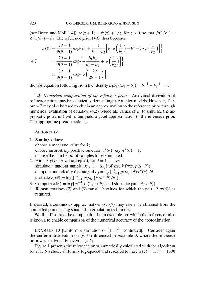
EXAMPLE 10 [Uniform distribution on (θ, θ2), continued]. Consider againthe uniform distribution on (θ, θ2) discussed in Example 9, where the referenceprior was analytically given in (4.7).

Figure 1 presents the reference prior numerically calculated with the algorithmfor nine θ values, uniformly log-spaced and rescaled to have π(2) = 1; m = 1000


FIG. 1. Numerical reference prior for the uniform model on [θ, θ2].

samples of k = 500 observations were used to compute each of the nine {θi, π(θi)}points. These nine points are clearly almost perfectly fitted by the exact referenceprior (4.7), shown by a continuous line; indeed, the nine points were accurate towithin four decimal points.

This numerical computation was done before the analytic reference prior wasobtained for the problem, and a nearly perfect fit to the nine θ values was obtainedby the function π(θ) = 1/(θ − 1), which was thus guessed to be the actual refer-ence prior. This guess was wrong, but note that (4.7) over the computed range isindeed nearly proportional to 1/(θ − 1).

We now consider an example for which the reference prior is not known and,indeed, appears to be extremely difficult to determine analytically.

EXAMPLE 11 (Triangular distribution). The use of a symmetric triangular dis-tribution on (0,1) can be traced back to the 18th century to Simpson [39]. Schmidt[37] noticed that this pdf is the density of the mean of two i.i.d. uniform randomvariables on the interval (0,1).

The nonsymmetric standard triangular distribution on (0,1),

p(x | θ) ={

2x/θ, for 0 < x ≤ θ ,2(1 − x)/(1 − θ), for θ < x < 1,

0 < θ < 1,

was first studied by Ayyangar [1]. Johnson and Kotz [33] revisited nonsymmetrictriangular distributions in the context of modeling prices. The triangular densityhas a unique mode at θ and satisfies Pr[x ≤ θ ] = θ , a property that can be used toobtain an estimate of θ based on the empirical distribution function. The nonsym-metric triangular distribution does not possess a useful reduced sufficient statistic.


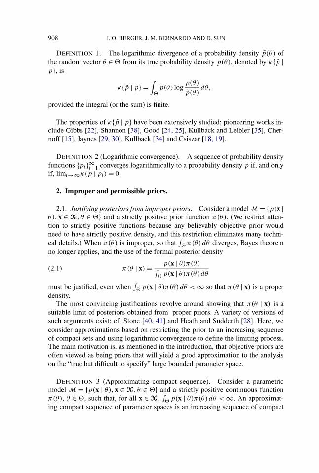
FIG. 2. Numerical reference prior for the triangular model.

Also, although log[p(x | θ)] is differentiable for all θ values, the formal Fisherinformation function is strictly negative, so Jeffreys prior does not exist.

Figure 2 presents a numerical calculation of the reference prior at thirteen θ

values, uniformly spaced on (0,1) and rescaled to have π(1/2) = 2/π ; m = 2500samples of k = 2000 observations were used to compute each of the thirteen{θi, π(θi)} points. Interestingly, these points are nearly perfectly fitted by the(proper) prior π(θ) = Be(θ | 1/2,1/2) ∝ θ−1/2(1 − θ)−1/2, shown by a continu-ous line.

Analytical derivation of the reference prior does not seem to be feasible in thisexample, but there is an interesting heuristic argument which suggests that theBe(θ | 1/2,1/2) prior is indeed the reference prior for the problem. The argumentbegins by noting that, if θ̃k is a consistent, asymptotically sufficient estimator of θ ,one would expect that, for large k,∫

Tp(tk | θ) log[π0(θ | tk)]dtk ≈

∫T

p(θ̃k | θ) log[π0(θ | θ̃k)]dθ̃k

≈ log[π0(θ | θ̃k)]|θ̃k=θ ,

since the sampling distribution of θ̃k will concentrate on θ . Thus, using (4.2) and(4.3), the reference prior should be

π(θ) = π0(θ | θ̃k)|θ̃k=θ ∝ p(θ̃k | θ)|θ̃k=θ .(4.8)

For the triangular distribution, a consistent estimator of θ can be obtained asthe solution to the equation Fk(t) = t , where Fk(t) is the empirical distributionfunction corresponding to a random sample of size k. Furthermore, one can showthat this solution, θ∗

k , is asymptotically normal N(θ∗k | θ, s(θ)/

√k), where s(θ) =√

θ(1 − θ). Plugging this into (4.8) would yield the Be(θ | 1/2,1/2) prior as the


reference prior. To make this argument precise, of course, one would have to verifythat the above heuristic argument holds and that θ∗

k is asymptotically sufficient.

5. Conclusions and generalizations. The formalization of the notions of per-missibility and the MMI property—the two keys to defining a reference prior—areof interest in their own right, but happened to be a by-product of the main goal,which was to obtain the explicit representation of a reference prior given in The-orem 7. Because of this explicit representation and, as illustrated in the examplesfollowing the theorem, one can:

• Have a single expression for calculating the reference prior, regardless of theasymptotic nature of the posterior distribution.

• Avoid the need to do computations over approximating compact parameterspaces.

• Develop a fairly simple numerical technique for computing the reference priorin situations where analytic determination is too difficult.

• Have, as immediate, the result that the reference prior on any compact subset ofthe parameter space is simply the overall reference prior constrained to that set.

The main limitation of the paper is the restriction to single parameter models.It would obviously be very useful to be able to generalize the results to deal withnuisance parameters.

The results concerning permissibility essentially generalize immediately to themulti-parameter case. The MMI property (and hence formal definition of a refer-ence prior) can also be generalized to the multi-parameter case, following Bergerand Bernardo [7] (although note that there were heuristic elements to that gen-eralization). The main motivation for this paper, however, was the explicit repre-sentation for the reference prior that was given in Theorem 7, and, unfortunately,there does not appear to be an analogue of this explicit representation in the multi-parameter case. Indeed, we have found that any generalizations seem to requireexpressions that involve limits over approximating compact sets, precisely the fea-ture of reference prior computation that we were seeking to avoid.

APPENDIX A: PROOF OF THEOREM 2

By the invariance of the model, p(x) = ∫� f (x − θ)π(θ) dθ = 1 and π(θ | x) =

f (x − θ). To verify (ii) of Definition 5, choose �i = [−i, i]. Then πi(θ | x) =f (x − θ)/[2ipi(x)], θ ∈ �i , where

pi(x) = 1

2i

∫ i

−if (x − θ) dθ = 1

2i

(F(x + i) − F(x − i)

),

with F(x) = ∫ x−∞ f (t) dt . The logarithmic discrepancy between πi(θ | x) and

π(θ | x) is

κ{π(· | x) | πi(· | x)} =∫ i

−iπi(θ | x) log

πi(θ | x)

π(θ | x)dθ


=∫ i

−iπi(θ | x) log

1

2ipi(x)dθ

= − log[F(x + i) − F(x − i)],and the expected discrepancy is∫ ∞

−∞κ{π(· | x) | πi(· | x)}pi(x) dx

= − 1

2i

∫ ∞−∞

[F(x + i) − F(x − i)] log[F(x + i) − F(x − i)]dx

=∫ −4

−∞g(y, i) dy +

∫ 2

−4g(y, i) dy +

∫ ∞2

g(y, i) dy = J1 + J2 + J3,

where, using the transformation y = (x − i)/i,

g(y, i) = −{F [(y + 2)i] − F(yi)} log{F [(y + 2)i] − F(yi)}.Notice that for fixed y ∈ (−4,2), as i → ∞,

F [(y + 2)i] − F(yi) →⎧⎨⎩

0, if y ∈ (−4,−2),1, if y ∈ (−2,0),0, if y ∈ (0,2).

Since −v logv ≤ e−1 for 0 ≤ v ≤ 1, the dominated convergence theorem can beapplied to J2, so that J2 converges to 0 as i → ∞. Next, when i is large enoughand, for any y ≥ 2,

F [(y + 2)i] − F(yi) ≤∫ (y+2)i

yi

1

t1+εdt = 1

ε

(1

(yi)ε− 1

[(y + 2)i]ε)

= (1 + 2/y)ε − 1

εiε(y + 2)ε≤ 2ε

iεy(y + 2)ε

the last inequality holding since, for 0 ≤ v ≤ 1, (1 + v)ε − 1 ≤ ε2ε−1v. Using thefact that −v logv is monotone increasing in 0 ≤ v ≤ e−1, we have

J3 ≤ −1

2

∫ ∞2

2ε

iεy(y + 2)εlog

2ε

iεy(y + 2)εdy,

which converges to 0 as i → ∞. It may similarly be shown that J1 converges to 0as i → ∞. Consequently, {πi(θ | x)}∞i=1 is expected logarithmically convergent toπ(θ | x), and thus, π(θ) = 1 is permissible.

APPENDIX B: DERIVATION OF RESULTS IN EXAMPLE 3

Consider a location family, p(x | θ) = f (x − θ), where x ∈ R and θ ∈ � = R,and f is given by f (x) = x−1(logx)−21(e,∞)(x). Choose π(θ) = 1 and �0 =


[a, b] such that L ≡ b − a ≥ 1. Then,

Lp0(x) =∫ b

af (x − θ) dθ

=

⎧⎪⎪⎪⎪⎨⎪⎪⎪⎪⎩

1

log(−b − x)− 1

log(−a − x), if x ≤ −b − e,

1 − 1

log(−a − x), if −b − e < x ≤ −a − e,

0, if x > −a − e.

The logarithmic discrepancy between π0(θ | x) and π(θ | x) is

κ{π(· | x) | π0(· | x)} =∫ b

aπ0(θ | x) log

π0(θ | x)

π(θ | x)dθ

=∫ b

aπ0(θ | x) log

1

Lp0(x)dθ = − log[Lp0(x)].

Then the expected discrepancy is

Ex0 κ{π(· | x) | π0(· | x)}

≡∫ ∞−∞

p0(x)κ{π(· | x) | π0(· | x)}dx

= − 1

L

∫ ∞−∞

Lp0(x) log[Lp0(x)]dx

≥ − 1

L

∫ −b−e

−∞

{1

log(−b − x)− 1

log(−a − x)

}

× log{

1

log(−b − x)− 1

log(−a − x)

}dx

= − 1

L

∫ ∞e

{1

log(t)− 1

log(t + L)

}log

{1

log(t)− 1

log(t + L)

}dt

≥ − 1

L

∫ ∞Le

{∫ t+L

t

1

x log2(x)dx

}log

{∫ t+L

t

1

x log2(x)dx

}dt.

Making the transformation y = t/L, the right-hand side equals

−∫ ∞e

gL(y) log{gL(y)}dy,

where

gL(y) =∫ (y+1)L

yL

1

x(logx)2 dx = 1

log(yL)− 1

log((y + 1)L)

= 1

log(y) + log(L)− 1

log(y) + log(1 + 1/y) + log(L)


= log(1 + 1/y)

[log(y) + log(L)][log(y + 1) + log(L)] .Because log(1 + 1/y) > 1/(y + 1), for y ≥ e,

gL(y) ≥ 1

(y + 1)[log(y + 1) + log(L)]2 .

Since −p log(p) is an increasing function of p ∈ (0, e−1), it follows that

Ex0 κ{π(· | x) | π0(· | x)} ≥ J1 + J2,

where

J1 =∫ ∞e

log(y + 1)

(y + 1)[log(y + 1) + log(L)]2 dy,

J2 =∫ ∞e

2 log[log(y + 1) + log(L)](y + 1)[log(y + 1) + log(L)]2 dy.

Clearly J1 = ∞ and J2 is finite, so Ex0 κ{π(· | x) | π0(· | x)} does not exist.

APPENDIX C: PROOF OF THEOREM 3

First,∫X1×X2

κ{π(· | x1,x2) | π0(· | x1,x2)}m0(x1,x2) dx1 dx2

=∫X1×X2

∫�0

log{π0(θ | x1,x2)

π(θ | x1,x2)

}π0(θ)p(x1,x2 | θ) dθ dx1 dx2

=∫X1×X2

∫�0

log{

π0(θ)m(x1,x2)

π(θ)m0(x1,x2)

}π0(θ)p(x1,x2 | θ) dθ dx1 dx2

=∫�0

log{π0(θ)

π(θ)

}π0(θ) dθ

(C.1)

+∫X1×X2

log{

m(x1,x2)

m0(x1,x2)

}m0(x1,x2) dx1 dx2

= J0 +∫X1

∫X2

log{

m(x2 | x1)m(x1)

m0(x2 | x1)m0(x1)

}

× m0(x2 | x1)m0(x1) dx1 dx2

≡ J0 + J1 + J2,

where J0 = ∫�0

log{π0(θ)/π(θ)}π0(θ) dθ ,

J1 =∫X1

log{

m(x1)

m0(x1)

}m0(x1) dx1,

J2 =∫X1

(∫X2

log{

m(x2 | x1)

m0(x2 | x1)

}m0(x2 | x1) dx2

)m0(x1) dx1.


By assumption, J0 is finite. Note that both m0(x2 | x1) and m(x2 | x1) =m(x1,x2)/m(x1) = ∫

� p(x2 | x1, θ)π(θ) dθ are proper densities. Because log(t)

is concave on (0,∞), we have

J2 ≤∫X1

log{∫

X2

m(x2 | x1)

m0(x2 | x1)m0(x2 | x1) dx2

}m0(x1) dx1 = 0.

By the same argument leading to (C.1), one can show that∫X1

κ{π(· | x1) | π0(· | x1)}m0(x1) dx1 = J0 + J1.

The result is immediate.

APPENDIX D: PROOF OF LEMMA 1

Clearly

I {p0 | Mk} ≡∫�0

p0(θ)

∫Tk

p(tk | θ) log[p0(θ | tk)

p0(θ)

]dtk dθ

=∫�0

p0(θ)

∫Tk

p(tk | θ) log[p(tk | θ)

p0(tk)

]dtk dθ

≤ supθ∈�0

∫Tk


p0(tk)

]dtk.

Writing p0(tk) = ∫�0

p(tk | θ ′)p0(θ′) dθ ′, note by convexity of [− log] that

∫Tk


p0(tk)

]dtk

= −∫Tk

p(tk | θ) log[∫

�0

p(tk | θ ′)p(tk | θ)

p0(θ′) dθ ′

]dtk

≤ −∫Tk

p(tk | θ)

[∫�0

log[p(tk | θ ′)p(tk | θ)

]p0(θ

′) dθ ′]dtk

= −∫�0

∫Tk

p(tk | θ) log[p(tk | θ ′)p(tk | θ)

]dtkp0(θ

′) dθ ′

≤ − infθ ′∈�0

∫Tk

p(tk | θ) log[p(tk | θ ′)p(tk | θ)

]dtk.

Combining this with (D.1) yields

I {p0 | Mk} ≤ supθ∈�0

supθ ′∈�0

∫Tk

p(tk | θ) log[

p(tk | θ)

p(tk | θ ′)

]dtk,

from which the result follows.


APPENDIX E: PROOF OF LEMMA 2

Let p0(θ | tk) be the posterior of θ under p0, that is, p(tk | θ)p0(θ)/p0(tk).Note that

I {p0 | Mk} ≡∫�0

p0(θ)

∫Tk


p0(θ)

]dtk dθ

=∫�0

∫Tk

p0(θ)p(tk | θ) log[p(tk | θ)

p0(tk)

]dtk dθ

=∫�0

p0(θ)

∫Tk

p(tk | θ) log[p(tk | θ)]dtk dθ

−∫Tk

p0(tk) log[p0(tk)]dtk.

Because I {p0 | Mk} ≥ 0,∫Tk

p0(tk) log[p0(tk)]dtk ≤∫�0

p0(θ)

∫Tk

p(tk | θ) log[p(tk | θ)]dtk dθ.

Condition (i) and the continuity of p ensure the right-hand side of the last equationis bounded above, and condition (ii) ensures that its left-hand side is boundedbelow. Consequently, I {p0 | Mk} < ∞.

APPENDIX F: PROOF OF THEOREM 7

For any p(θ) ∈ Ps , denote the posterior corresponding to p0 (the restriction ofp to the compact set �0) by p0(θ | tk).

Step 1. We give an expansion of I {p0 | Mk}, defined by

I {p0 | Mk} =∫�0

p0(θ)

∫Tk


p0(θ)

]dtk dθ.

Use the equality

p0(θ | tk)p0(θ)

= p0(θ | tk)π∗

0 (θ | tk)π∗

0 (θ | tk)π∗(θ | tk)

π∗(θ | tk)π∗

0k(θ)

π∗0k(θ)

p0(θ),

where

π∗0k(θ) = fk(θ)

c0(fk)1�0(θ) and c0(fk) =

∫�0

fk(θ) dθ.(F.1)

We have the decomposition

I {p0 | Mk} =4∑

j=1

Gjk,(F.2)


where

G1k = −∫�0

p0(θ)

∫Tk

p(tk | θ) log[π∗

0 (θ | tk)p0(θ | tk)

]dθ dtk,

G2k =∫�0

p0(θ)

∫Tk


0 (θ | tk)π∗(θ | tk)

]dtk dθ,

G3k =∫�0

p0(θ)

∫Tk

p(tk | θ) log[π∗(θ | tk)π∗

0k(θ)

]dtk dθ,

G4k =∫�0

p0(θ)

∫Tk


0k(θ)

p0(θ)

]dtk dθ.

It is easy to see that

G3k =∫�0

p0(θ) log[

fk(θ)

π∗0k(θ)

]dθ.

From (F.1), fk(θ)/π∗0k(θ) = c0(fk) on �0. Then,

G3k = log[c0(fk)].(F.3)

Clearly,

G4k = −∫�0

p0(θ) log[

p0(θ)

π∗0k(θ)

]dθ.(F.4)

Note that the continuity of p(tk | θ) in θ and integrability will imply the continuityof fk . So, π∗

0k is continuous and bounded, and G4k is finite. Since, 0 ≤ I {p0 |Mk} < ∞, Gjk, j = 1,2,3 are all nonnegative and finite.

Step 2. We show that

limk→∞G1k = 0 ∀p ∈ Ps .(F.5)

It is easy to see

π∗0 (θ | tk)

p0(θ | tk)= π∗(θ)

p(θ)

∫�0

p(tk | τ)p(τ) dτ∫�0

p(tk | τ)π∗(τ ) dτ

= π∗(θ)

p(θ)

∫�0

p(tk | τ)p(τ) dτ∫� p(tk | τ)π∗(τ ) dτ

[P ∗(�0 | tk)]−1.(F.6)

The definition of posterior consistency of π∗ is that, for any θ ∈ � and any ε > 0,

P ∗(|τ − θ | ≤ ε | tk) ≡∫{τ :|τ−θ |≤ε}

π∗(τ | tk) dτP−→ 1,(F.7)

in probability p(tk | θ) as k → ∞. It is immediate that

P ∗(�0 | tk) =∫�0

p(tk | τ)π∗(τ ) dτ∫� p(tk | τ)π∗(τ ) dτ

P−→ 1,(F.8)


with probability p(tk | θ) as θ ∈ �0 and k → ∞. Because both π∗ and p arecontinuous, for any ε > 0, there is small δ > 0, such that

∣∣∣∣ p(τ)

π∗(τ )− p(θ)

π∗(θ)

∣∣∣∣ ≤ ε ∀τ ∈ �0 ∩ (θ − δ, θ + δ)(F.9)

For such a δ, we could write

π∗(θ)

p(θ)

∫�0

p(tk | τ)p(τ) dτ∫� p(tk | τ)π∗(τ ) dτ

≡ J1k + J2k,(F.10)

where

J1k = π∗(θ)

p(θ)

∫�0∩(θ−δ,θ+δ) p(tk | τ)(p(τ)/π∗(τ ))π∗(τ ) dτ∫

� p(tk | τ)π∗(τ ) dτ,

J2k = π∗(θ)

p(θ)

∫�0∩(θ−δ,θ+δ)c p(tk | τ)(p(τ)/π∗(τ ))π∗(τ ) dτ∫

� p(tk | τ)π∗(τ ) dτ.

Clearly, (F.9) implies that

J1k ≥ π∗(θ)

p(θ)

[p(θ)

π∗(θ)− ε

]∫�0∩(θ−δ,θ+δ)

π∗(τ | tk) dτ,

J1k ≤ π∗(θ)

p(θ)

[p(θ)

π∗(θ)+ ε

]∫�0∩(θ−δ,θ+δ)

π∗(τ | tk) dτ.

(F.7) implies that, for the fixed δ and θ ∈ �0,[1 − ε

π∗(θ)

p(θ)

]≤ J1k ≤

[1 + ε

π∗(θ)

p(θ)

](F.11)

with probability p(tk | θ) as k → ∞. Noting that p(θ) is continuous and positiveon �0, let M1 > 0 and M2 be the lower and upper bounds of p on �0. From (F.7),

0 ≤ J2k ≤ M2π∗(θ)

M1p(θ)

∫�0∩(θ−δ,θ+δ)c

π∗(τ | tk) dτP−→ 0,(F.12)

with probability p(tk | θ) as k → ∞. Combining (F.6), (F.8) and (F.10)–(F.12), weknow that

π∗0 (θ | tk)

p0(θ | tk)P−→ 1(F.13)

with probability p(tk | θ) as k → ∞. It is easy to see that the left quantity of (F.13)is bounded above and below, so the dominated convergence theorem implies (F.5).


G5k ≡∫�0

π∗0 (θ)

∫Tk

p(tk | θ) logπ∗

0 (θ | tk)π∗(θ | tk)

dtk dθ → 0 as k → ∞.(F.14)


For any measurable set A ⊂ R, denote P ∗(A | tk) = ∫A π∗(θ | tk) dθ . Then,

π∗0 (θ | tk)

π∗(θ | tk)= p(tk | θ)π∗

0 (θ)/p∗0(tk)

p(tk | θ)π∗(θ)/p∗(tk)=

∫� p(tk | θ)π∗(θ) dθ∫�0

p(tk | θ)π∗(θ) dθ

= 1 +∫�c

0p(tk | θ)π∗(θ) dθ∫

�0p(tk | θ)π∗(θ) dθ

= 1 + P ∗(�c0 | tk)

P ∗(�0 | tk).

Thus,

G5k =∫�0

π∗0 (θ)

∫Tk

p(tk | θ) log{

1 + P ∗(�c0 | tk)

P ∗(�0 | tk)

}dtk dθ.

For any 0 ≤ a ≤ b ≤ ∞, denote

Tk,a,b ={

tk :a ≤ P ∗(�c0 | tk)

P ∗(�0 | tk)< b

}.(F.15)

Clearly, if 0 < ε < M < ∞,

Tk = Tk,0,ε ∪ Tk,ε,M ∪ Tk,M,∞.

We then have the decomposition for G5k ,

G5k ≡ G5k1 + G5k2 + G5k3,(F.16)

where

G5k1 =∫�0

π∗0 (θ)

∫Tk,0,ε

p(tk | θ) log{

1 + P ∗(�c0 | tk)

P ∗(�0 | tk)

}dtk dθ,

G5k2 =∫�0

π∗0 (θ)

∫Tk,ε,M

p(tk | θ) log{

1 + P ∗(�c0 | tk)

P ∗(�0 | tk)

}dtk dθ,

G5k3 =∫�0

π∗0 (θ)

∫Tk,M,∞

p(tk | θ) log{

1 + P ∗(�c0 | tk)

P ∗(�0 | tk)

}dtk dθ.

The posterior consistency (F.8) implies that if θ ∈ �00 (the interior of �0),

P ∗(�c0 | tk)

P−→ 0,(F.17)

in probability p(tk | θ) as k → ∞. So (F.17) implies that, for any small ε > 0 andany fixed θ ∈ �0

0, ∫Tk,ε,∞

p(tk | θ) dtk −→ 0 as k → ∞.(F.18)

For small ε > 0,

G5k1 ≤ log(1 + ε)

∫�0

π∗0 (θ)

∫Tk,0,ε

p(tk | θ) dtk dθ

≤ log(1 + ε) < ε.


For any large M > max(ε, e − 1),

G5k2 ≤ log(1 + M)

∫�0

π∗0 (θ)

∫Tk,ε,M

p(tk | θ) dtk dθ

≤ log(1 + M)

∫�0

π∗0 (θ)

∫Tk,ε,∞

p(tk | θ) dtk dθ.

Since π∗0 is bounded on �0, (F.18) and dominated convergence theorem imply that

G5k2 → 0 as k → ∞.

Also,

G5k3 =∫�0

π∗0 (θ)

∫Tk,M,∞

p(tk | θ) log{

1

P ∗(�0 | tk)

}dtk dθ

= − 1

c0(π∗)

∫Tk,M,∞

p∗(tk)∫�0

p∗(θ | tk) log[P ∗(�0 | tk)]dθ dtk

= − 1

c0(π∗)

∫Tk,M,∞

p∗(tk)P ∗(�0 | tk) log[P ∗(�0 | tk)]dtk.

Note that tk ∈ Tk,M,∞ if and only if P ∗(�0 | tk) < 1/(1 + M). Also, −p log(p) isincreasing for p ∈ (0,1/e). This implies that

−P ∗(�0 | tk) log[P ∗(�0 | tk)] <1

1 + Mlog(1 + M).

Consequently,

J5k ≤ 1

c0(π∗)(1 + M)log(1 + M)

∫Tk,M,∞

p∗(tk) dtk

≤ 1

c0(π∗)(1 + M)log(1 + M).

Now for fixed small ε > 0, we could choose M > max(ε, e − 1) large enough sothat G5k3 ≤ ε. For such fixed ε and M , we know G5k2 → 0 as k → ∞. Since ε isarbitrary, (F.14) holds.


limk→∞G2k = 0 ∀p ∈ Ps .(F.19)

Note that for any p ∈ Ps , there is a constant M > 0, such that

supτ∈�0

p0(τ )

π∗0 (τ )

≤ M.

Since π∗0 (θ | tk)/π∗(θ | tk) ≥ 1,

0 ≤ G2k ≤ M

∫�0

π∗0 (θ)

∫Tk


0 (θ | tk)π∗(θ | tk)

]dtk dθ = MG5k.


Then, (F.14) implies (F.19) immediately.Step 5. It follows from (F.2) that for any prior p ∈ Ps ,

I {π0 | Mk} − I {p0 | Mk}= −G1k − G2k +

∫�0

π0(θ)

∫Tk


0 (θ | tk)π∗(θ | tk)

]dtk dθ

−∫�0

π0(θ) log[

π0(θ)

π∗0k(θ)

]dθ +

∫�0

p0(θ) log[

p0(θ)

π∗0k(θ)

]dθ.

Steps 2 and 4 imply that

limk→∞(I {π0 | Mk} − I {p0 | Mk}) = lim

k→∞

{−

∫�0

π0(θ) log[

π0(θ)

π∗0k(θ)

]dθ

+∫�0

p0(θ) log[

p0(θ)

π∗0k(θ)

]dθ

}(F.20)

≥ − limk→∞

∫�0

π0(θ) log[

π0(θ)

π∗0k(θ)

]dθ,

the last inequality holding since the second term is always nonnegative. Finally,

limk→∞

∫�0

π0(θ) log[π∗0k(θ)]dθ

= limk→∞

∫�0

π0(θ) log[

fk(θ)

c0(fk)

]dθ

= limk→∞

∫�0

π0(θ) log[

fk(θ)

fk(θ0)

fk(θ0)

c0(fk)

]dθ

= limk→∞

∫�0

π0(θ) log[

fk(θ)

fk(θ0)

]dθ + lim

k→∞ log[fk(θ0)

c0(fk)

]

=∫�0

π0(θ) log[f (θ)]dθ − log[c0(f )]

=∫�0

π0(θ) log[π0(θ)]dθ,

the second to last line following from condition (i) and

limk→∞

c0(fk)

fk(θ0)= lim

k→∞

∫�0

fk(θ)

fk(θ0)dθ

=∫�0

limk→∞

fk(θ)

fk(θ0)dθ =

∫�0

f (θ) dθ = c0(f ).

Consequently, the right-hand side of (F.20) is 0, completing the proof.


APPENDIX G: PROOF OF THEOREM 8

Let x(k) = {x1, . . . , xk} consist of k replications from the original uniformdistribution on the interval (a1(θ), a2(θ)). Let t1 = tk1 = min{x1, . . . , xk} andt2 = tk2 = max{x1, . . . , xk}. Clearly, tk ≡ (t1, t2) are sufficient statistics with den-sity

p(t1, t2 | θ) = k(k − 1)(t2 − t1)k−2

[a2(θ) − a1(θ)]k , a1(θ) < t1 < t2 < a2(θ).(G.1)

Choosing π∗(θ) = 1, the corresponding posterior density of θ is

π∗(θ | t1, t2) = 1

[a2(θ) − a1(θ)]kmk(t1, t2),

(G.2)a−1

2 (t2) < θ < a−11 (t1),

where

mk(t1, t2) =∫ a−1

1 (t1)

a−12 (t2)

1

[a2(s) − a1(s)]k ds.(G.3)

Consider the transformation

y1 = k(a−1

1 (t1) − θ)

and y2 = k(θ − a−1

2 (t2)),(G.4)

or equivalently, t1 = a1(θ + y1/k) and t2 = a2(θ − y2/k).We first consider the frequentist asymptotic distribution of (y1, y2). For θ > θ0,

we know a1(θ) < a2(θ). For any fixed y1 > 0 and y2 > 0, a1(θ + y1/k) < a2(θ −y2/k) when k is large enough. From (G.1), the joint density of (y1, y2) is

p(y1, y2 | θ)

= (k − 1)

k

a′1(θ + y1/k)a′

2(θ − y2/k)

[a2(θ) − a1(θ)]k{a2

(θ − y2

k

)2

− a1

(θ + y1

k

)}k−2

= (k − 1)

k

a′1(θ + y1/k)a′

2(θ − y2/k)

[a2(θ) − a1(θ)]2

×{

1 − a′1(θ)y1 + a′

2(θ)y2

[a2(θ) − a1(θ)]k + o

(1

k

)}k−2

.

For fixed θ > θ0, y1, y2 > 0, as k → ∞,

p(y1, y2 | θ) → a′1(θ)a′

2(θ)

[a2(θ) − a1(θ)]2 exp{−a′

1(θ)y1 + a′2(θ)y2

a2(θ) − a1(θ)

}

(G.5)≡ p∗(y1, y2 | θ).

Consequently, as k → ∞, the yi ’s have independent exponential distributions withmeans λi = [a2(θ) − a1(θ)]/a′

i(θ).


With the transformation (G.4),

mk(t1, t2) =∫ θ+y1/k

θ−y2/k

1

[a2(s) − a1(s)]k ds

(G.6)

= 1

k

∫ y1

−y2

1

[a2(θ + v/k) − a1(θ + v/k)]k dv.

So, for any fixed y1, y2 > 0 as k → ∞,

k[a2(θ) − a1(θ)]kmk(t1, t2)

−→∫ y1

−y2

exp[−a′

2(θ) − a′1(θ)

a2(θ) − a1(θ)v

]dv

= a2(θ) − a1(θ)

a′2(θ) − a′

1(θ)exp

[a′

2(θ) − a′1(θ)

a2(θ) − a1(θ)y2

]

×{

1 − exp[−a′

2(θ) − a′1(θ)

a2(θ) − a1(θ)(y1 + y2)

]}.

Then, for fixed θ > θ0 as k → ∞,∫log(π(θ | t1, t2))f (t1, t2 | θ) dt1 dt2 − log(k)

(G.7)

−→ log{a′

2(θ) − a′1(θ)

a2(θ) − a1(θ)

}+ J1(θ) + J2(θ),

where

J1(θ) = a′2(θ) − a′

1(θ)

a2(θ) − a1(θ)

∫ ∞0

∫ ∞0

y2p∗(y1, y2 | θ) dy1 dy2,

J2(θ) = −∫ ∞

0

∫ ∞0

log{

1 − exp[−a′

2(θ) − a′1(θ)

a2(θ) − a1(θ)(y1 + y2)

]}

× p∗(y1, y2 | θ) dy1 dy2.

It follows from (G.5) that

J1(θ) = −b2,

J2(θ) = −E log{1 − e−b1V1e−b2V2},where V1 and V2 are i.i.d. with the standard exponential distribution. Then,

J2(θ) =∞∑

j=1

1

jE(e−jb1V1)E(e−jb2V2)

=∞∑

j=1

1

j (b1j + 1)(b2j + 1)(G.8)


= 1

b1 − b2

∞∑j=1

1

j

(1

j + 1/b1− 1

j + 1/b2

).

Note that the digamma function ψ(z) satisfies the equation,

∞∑j=1

1

j (j + z)= ψ(z + 1) + γ

z,(G.9)

for z > 0, where γ is the Euler–Mascherono constant (see, e.g., Boros and Moll[14].) Equations (G.8) and (G.9) imply that

J2(θ) = 1

b1 − b2

{b1

[ψ

(1

b1+ 1

)+ γ

]− b2

[ψ

(1

b2+ 1

)+ γ

]}

= γ + 1

b1 − b2

{b1ψ

(1

b1+ 1

)− b2ψ

(1

b2+ 1

)}.

Using the fact that ψ(z + 1) = ψ(z) + 1/z,

J1(θ) + J2(θ) = γ − b2 + 1

b1 − b2

{b2

1 + b1ψ

(1

b1

)− b2

2 − b2ψ

(1

b2

)}

(G.10)

= γ + b1 + 1

b1 − b2

{b1ψ

(1

b1

)− b2ψ

(1

b2

)}.

The result follows from (G.7) and (G.10).

Acknowledgments. The authors are grateful to Susie Bayarri for helpful dis-cussions. The authors acknowledge the constructive comments of the AssociateEditor and referee.

REFERENCES

[1] AYYANGAR, A. S. K. (1941). The triangular distribution. Math. Students 9 85–87.MR0005557

[2] BERGER, J. O. (1985). Statistical Decision Theory and Bayesian Analysis, 2nd ed. Springer,Berlin. MR0804611

[3] BERGER, J. O. (2006). The case for objective Bayesian analysis (with discussion). BayesianAnal. 1 385–402 and 457–464. MR2221271

[4] BERGER, J. O. and BERNARDO, J. M. (1989). Estimating a product of means: Bayesian analy-sis with reference priors. J. Amer. Statist. Assoc. 84 200–207. MR0999679

[5] BERGER, J. O. and BERNARDO, J. M. (1992a). Ordered group reference priors with applica-tions to a multinomial problem. Biometrica 79 25–37. MR1158515

[6] BERGER, J. O. and BERNARDO, J. M. (1992b). Reference priors in a variance componentsproblem. In Bayesian Analysis in Statistics and Econometrics (P. K. Goel and N. S. Iyen-gar, eds.) 323–340. Springer, Berlin. MR1194392

[7] BERGER, J. O. and BERNARDO, J. M. (1992c). On the development of reference priors (withdiscussion). In Bayesian Statistics 4 (J. M. Bernardo, J. O. Berger, A. P. Dawid and A. F.M. Smith, eds.) 35–60. Oxford Univ. Press. MR1380269

http://www.ams.org/mathscinet-getitem?mr=0005557








[8] BERGER, J. O., DE OLIVEIRA, V. and SANSÓ, B. (2001). Objective Bayesian analysis ofspatially correlated data. J. Amer. Statist. Assoc. 96 1361–1374. MR1946582

[9] BERGER, J. O. and YANG, R. (1994). Noninformative priors and Bayesian testing for theAR(1) model. Econometric Theory 10 461–482. MR1309107

[10] BERNARDO, J. M. (1979). Reference posterior distributions for Bayesian inference (with dis-cussion). J. Roy. Statist. Soc. Ser. B 41 113–147. [Reprinted in Bayesian Inference (N. G.Polson and G. C. Tiao, eds.) 229–263. Edward Elgar, Brookfield, VT, 1995.] MR0547240

[11] BERNARDO, J. M. (2005). Reference analysis. In Handbook of Statistics 25 (D. K. Dey and C.R. Rao, eds.) 17–90. North-Holland, Amsterdam.

[12] BERNARDO, J. M. and RUEDA, R. (2002). Bayesian hypothesis testing: A reference approach.Internat. Statist. Rev. 70 351–372.

[13] BERNARDO, J. M. and SMITH, A. F. M. (1994). Bayesian Theory. Wiley, Chichester.MR1274699

[14] BOROS, G. and MOLL, V. (2004). The Psi function. In Irresistible Integrals: Symbolics,Analysis and Experiments in the Evaluation of Integral 212–215. Cambridge Univ. Press.MR2070237

[15] CHERNOFF, H. (1956). Large-sample theory: Parametric case. Ann. Math. Statist. 27 1–22.MR0076245

[16] CLARKE, B. (1999). Asymptotic normality of the posterior in relative entropy. IEEE Trans.Inform. Theory 45 165–176. MR1677856

[17] CLARKE, B. and BARRON, A. R. (1994). Jeffreys’ prior is asymptotically least favorable underentropy risk. J. Statist. Plann. Inference 41 37–60. MR1292146

[18] CSISZAR, I. (1967). Information-type measures of difference of probability distributions andindirect observations. Studia Sci. Math. Hungar. 2 299–318. MR0219345

[19] CSISZAR, I. (1975). I -divergence geometry of probability distributions and minimization prob-lems. Ann. Probab. 3 146–158. MR0365798

[20] DATTA, G. S. and MUKERJEE, R. (2004). Probability Matching Priors: Higher Order As-ymptotics. Springer, New York. MR2053794

[21] FRASER, D. A. S., MONETTE, G. and NG, K. W. (1985). Marginalization, likelihood andstructural models. In Multivariate Analysis 6 (P. R. Krishnaiah, ed.) 209–217. North-Holland, Amsterdam. MR0822296

[22] GIBBS, J. W. (1902). Elementary Principles in Statistical Mechanics. Constable, London.Reprinted by Dover, New York, 1960. MR0116523

[23] GHOSH, J. K., DELAMPADY, M. and SAMANTA, T. (2006). An Introduction to BayesianAnalysis: Theory and Methods. Springer, New York. MR2247439

[24] GOOD, I. J. (1950). Probability and the Weighing of Evidence. Hafner Press, New York.MR0041366

[25] GOOD, I. J. (1969). What is the use of a distribution? In Multivariate Analysis 2 (P. R. Krish-naiah, ed.) 183–203. North-Holland, Amsterdam. MR0260075

[26] GHOSAL, S. (1997). Reference priors in multiparameter nonregular cases. Test 6 159–186.MR1466439

[27] GHOSAL, S. and SAMANTA, T. (1997). Expansion of Bayes risk for entropy loss and referenceprior in nonregular cases. Statist. Decisions 15 129–140. MR1475184

[28] HEATH, D. L. and SUDDERTH, W. D. (1989). Coherent inference from improper priors andfrom finitely additive priors. Ann. Statist. 17 907–919. MR0994275

[29] JAYNES, E. T. (1957). Information theory and statistical mechanics. Phys. Rev. 106 620–630.MR0087305

[30] JAYNES, E. T. (1968). Prior probabilities. IEEE Trans. Systems, Science and Cybernetics 4227–291.

[31] JEFFREYS, H. (1946). An invariant form for the prior probability in estimation problems. Proc.Roy. Soc. London Ser. A 186 453–461. MR0017504























[32] JEFFREYS, H. (1961). Theory of Probability, 3rd ed. Oxford Univ. Press. MR0187257[33] JOHNSON, N. J. and KOTZ, S. (1999). Nonsmooth sailing or triangular distributions revisited

after some 50 years. The Statistician 48 179–187.[34] KULLBACK, S. (1959). Information Theory and Statistics, 2nd ed. Dover, New York.

MR0103557[35] KULLBACK, S. and LEIBLER, R. A. (1951). On information and sufficiency. Ann. Math. Sta-

tist. 22 79–86. MR0039968[36] LINDLEY, D. V. (1956). On a measure of information provided by an experiment. Ann. Math.

Statist. 27 986–1005. MR0083936[37] SCHMIDT, R. (1934). Statistical analysis if one-dimentional distributions. Ann. Math. Statist. 5

30–43.[38] SHANNON, C. E. (1948). A mathematical theory of communication. Bell System Tech. J. 27

379–423, 623–656. MR0026286[39] SIMPSON, T. (1755). A letter to the right honourable George Earls of Maclesfield. President

of the Royal Society, on the advantage of taking the mean of a number of observations inpractical astronomy. Philos. Trans. 49 82–93.

[40] STONE, M. (1965). Right Haar measures for convergence in probability to invariant posteriordistributions. Ann. Math. Statist. 36 440–453. MR0175213

[41] STONE, M. (1970). Necessary and sufficient condition for convergence in probability to invari-ant posterior distributions. Ann. Math. Statist. 41 1349–1353. MR0266359

[42] SUN, D. and BERGER, J. O. (1998). Reference priors under partial information. Biometrika85 55–71. MR1627242

[43] WASSERMAN, L. (2000). Asymptotic inference for mixture models using data-dependent pri-ors. J. Roy. Statist. Soc. Ser. B 62 159–180. MR1747402

J. O. BERGER

DEPARTMENT OF STATISTICAL SCIENCES

DUKE UNIVERSITY

BOX 90251DURHAM, NORTH CAROLINA 27708-0251USAE-MAIL: [email protected]: www.stat.duke.edu/~berger/

J. M. BERNARDO

DEPARTAMENTO DE ESTADÍSTICA

FACULTAD DE MATEMÁTICAS

46100–BURJASSOT

VALENCIA

SPAIN

E-MAIL: [email protected]: www.uv.es/~bernardo/

D. SUN

DEPARTMENT OF STATISTICS

UNIVERSITY OF MISSOURI-COLUMBIA

146 MIDDLEBUSH HALL

COLUMBIA, MISSOURI 65211-6100USAE-MAIL: [email protected]: www.stat.missouri.edu/~dsun/










mailto:[email protected]

http://www.stat.duke.edu/~berger/


http://www.uv.es/~bernardo/


http://www.stat.missouri.edu/~dsun/

Documents

The formal definition of reference priorsberger/papers/formal-def.pdf · THE FORMAL DEFINITION OF REFERENCE PRIORS BY JAMES O. BERGER,1 JOSÉ M. BERNARDO2 AND DONGCHU SUN3 Duke University,