The Formation of Financial Networks

Ana Babus∗

Federal Reserve Bank of Chicago

Abstract

Modern banking systems are highly interconnected. Despite various benefits, link-

ages between banks carry the risk of contagion. In this paper I investigate whether

banks can commit ex-ante to mutually insure each other, when there is contagion risk

in the financial system. I model banks’decisions to share this risk through bilateral

agreements. A financial network that allows losses to be shared among various coun-

terparties arises endogenously. I characterize the probability of systemic risk, defined

as the event that contagion occurs conditional on one bank failing, in equilibrium

interbank networks. I show that there exist equilibria in which contagion does not

occur.

Keywords: financial stability; network formation; contagion risk;

JEL: C70; G21.

∗E-mail: anababus@gmail.com. I am grateful to Franklin Allen, Douglas Gale, two anonymous referees

and the editor for very useful comments and guidance. The views in this papers are solely those of the

author and need not represent the views of the Federal Reserve Bank of Chicago or the Federal Reserve

System.

1

1 Introduction

The recent turmoils in financial markets have revealed, once again, the intertwined nature

of financial systems. In a modern financial world, banks and other institutions are linked

in a variety of ways. These connections often involve trade-offs. For instance, although

banks can solve their liquidity imbalances by borrowing and lending on the interbank

market, they expose themselves, at the same time, to contagion risk. How do banks weigh

these trade-offs, and what are the externalities of their decisions on the financial system

as a whole?

In this paper I explore whether banks can commit ex-ante to mutually insure each

other, when the failure of an institution introduces the risk of contagion in the financial

system. As a form of insurance, banks can hold mutual claims on one another. These

mutual claims are, essentially, bilateral agreements that allow losses to be shared among

all counterparties of a failed bank. The more bilateral agreements a bank has, the smaller

the loss that each of her counterparties incurs. Contagion does not take place provided

each bank has suffi ciently many bilateral agreements. I model banks’decision to share the

risk of contagion bilaterally as a network formation game. Various equilibria arise. In most

equilibria the financial system is resilient to the demise of some banks, but not the others.

Equilibria in which there is no contagion can be supported as well. Moreover, I show

that the welfare in equilibrium interbank networks is decreasing in the probability that

contagion occurs. However, more bilateral agreements between banks do not necessarily

improve welfare beyond the point when there is no contagion.

To study these issues, I build on the framework proposed by Allen and Gale (2000).

In particular, I consider a three-period model, where the banking system consists of two

identically sized regions. Banks raise deposits from consumers who are uncertain about

their liquidity preferences, as in Diamond and Dybvig (1983). Each region is subject

to liquidity shocks driven by consumers’liquidity needs. Liquidity shocks are negatively

correlated across the two regions. In addition, there is a small probability that one of

the banks, chosen at random, is affected by an early-withdrawal shock and liquidated

prematurely.

Banks can perfectly insure against liquidity shocks by exchanging interbank deposits

2

with banks in the other region. However, the connections created by swapping deposits

expose the system to contagion when the early-withdrawal shock realizes. The loss that

a bank induces when she is affected by the early-withdrawal shock is shared across her

counterparties. This implies that as banks exchange more deposits, the loss on every

deposit is smaller. The model predicts a connectivity threshold above which contagion does

not occur. Reaching this connectivity threshold may require that banks swap deposits with

other banks in the same region. I distinguish between a liquidity network, that smoothes

out liquidity shocks in the banking system, and a solvency network, that provides insurance

against contagion risk.

The distinction between liquidity links and solvency links is useful to study the incen-

tives that banks have to insure against contagion. In particular, I study whether banks

choose to form solvency links with other banks in the same region. When a bank has at

least as many links as the connectivity threshold requires, then no contagion takes place

if she is affected by the early-withdrawal shock. However, her counterparties still incur a

loss on their deposits. When deciding to form solvency links, banks are willing to incur

a small loss on their deposits, if they can avoid default. However, they are better off if

contagion is averted without incurring any cost. This implies that banks have the incen-

tive to free-ride on others’links. Because of this, many network structures can be stable

in which full financial stability is not necessarily achieved.

In the main specification of the model, I show that at least half of the banks have

swapped deposits with suffi ciently many other banks in the same region. In other words,

a systemic event in which all banks default if one bank is subject to an early-withdrawal

shock occurs in at most half of the cases. Even then, I find that insuring against regional

fluctuations in the fraction of early consumers through a liquidity network is optimal as

long as the probability of the early-withdrawal shock is suffi ciently small.

The equilibria in which all banks have suffi ciently many links and no contagion occurs

have the highest associated welfare. This is intuitive, as banks’ assets are ineffi ciently

liquidated if a systemic event occurs. However, in interbank networks in which contagion

does not occur, welfare is not necessarily increasing with the number of links that banks

have. This is because when each bank has more links, there are also more banks that

incur losses on their deposits. However, since banks have already suffi ciently many links,

3

there is no benefit to offset this implicit cost.

Thus, increasing the connectivity of the interbank network is beneficial up to the point

when there is no contagion in the financial system. The idea that an interconnected

banking system may be optimal is supported by various other studies. Leitner (2005)

discusses how the threat of contagion may be part of an optimal network design. His model

predicts that it is optimal for some agents to bail out other agents, in order to prevent the

collapse of the whole network. This form of insurance can also emerge endogenously, and

I show that it is an equilibrium in a network formation game. Linkages between banks

can also be effi cient in the model of Kahn and Santos (2008) if there is suffi cient liquidity

in the financial system. Recently, Acemoglu et al. (2015) find that the types of financial

networks that are most prone to contagious failures depend on the number of adverse

shocks that affect the financial system.

The rationale for why a bank is willing to form solvency links with other banks in

the same region and incur a loss on her deposits is that an early-withdrawal shock to any

bank can have system-wide externalities. In particular, all banks default when a bank

that has insuffi cient links is affected by an early-withdrawal shock. Banks are willing to

pay a premium (i.e. incur a loss on their deposits) to avoid defaulting by contagion. Thus,

a solvency interbank network can be interpreted as an alternative to formal insurance

markets. Moreover, the network formation approach provides insights about the circum-

stances in which banks are willing to purchase protection, as well as about the premia they

are willing to pay. From this perspective, the findings in this paper complement solutions

relying on formal insurance arrangements previously proposed in the literature. For in-

stance, Zawadowki (2013) shows, in the context of OTC traded contracts, that competitive

insurance markets fail as banks find the premia for insuring against counterparty default

too expensive. This is because banks do not internalize that the default of another bank

which is not an immediate neighbor can nevertheless affect them in subsequent default

waves. Insurance is unattractive in Kyiotaki and Moore (1997) as well, because of limited

enforcement of contracts. Similarly, it has been shown that other formal arrangements,

such as clearinghouses, may increase systemic risk either because they reduce netting ef-

ficiency (as in Duffi e and Zhu, 2011) or they reduce dealers’ incentives to monitor each

other (as in Pirrong, 2009).

4

Starting with Allen and Gale (2000) there has been a growing interest in how different

network structures respond to the breakdown of a single bank in order to identify which

ones are more fragile: See, for instance, the theoretical investigation of Freixas et al. (2000)

or Castiglionesi and Navarro (2007) , and the experimental study of Corbae and Duffy

(2008). In parallel, the empirical literature has looked for evidence of contagious failures

of financial institutions resulting from mutual claims they have on one another and has

shown such interbank loans are unlikely to lead to sizable contagion in developed markets

(Furfine, 2003; Upper and Worms, 2004). Other papers are concerned with whether

interbank markets anticipate contagion. For instance, in Dasgupta (2004) contagion arises

as an equilibrium outcome conditional on the arrival of negative interim information which

leads to coordination problems among depositors and widespread runs, whereas Caballero

and Simsek (2013) provide a model of market freezes when the complexity of a financial

network increases the uncertainty about the health of trading counterparties and of their

partners. More recently, Alvarez and Barlevy (2014) study mandatory disclosure of losses

at financial institutions which are exposed to contagion via a network of interbank loans.

This paper is organized as follows. Section 2 introduces the model in its generality.

Section 3 describes when contagion can occur and the payoffs that banks receive. Section

4 provides the equilibrium analysis. In section 5, I present an extension of the model to

include small linking costs and discuss welfare implications. Section 6 concludes.

2 The Model

2.1 Consumers and liquidity preferences

The economy is divided into 2n sectors, each populated by a continuum of consumers.

Consumers’ preferences are described by a log-utility function. There are three time

periods t = 0, 1, 2. Each agent is endowed with one unit of consumption good at date t = 0.

Agents are uncertain about their liquidity preferences: they can be early consumers, who

value consumption only at date 1, or they can be late consumers, who value consumption

only at date 2.

The probability that an agent is a early consumer is q. I assume that the law of large

numbers holds in the continuum, which implies that, on average, the fraction of agents

5

Region A Region B

Probability State/Sector 1 2 ... n n+ 1 n+ 2 ... 2n

(1− ϕ)/2 S1 pH pH ... pH pL pL ... pL

(1− ϕ)/2 S2 pL pL ... pL pH pH ... pH

q + χ q ... q q q ... q

ϕ S q q + χ ... q q q ... q

... ... ... ... ... ... ... ...

q q ... q q q ... q + χ

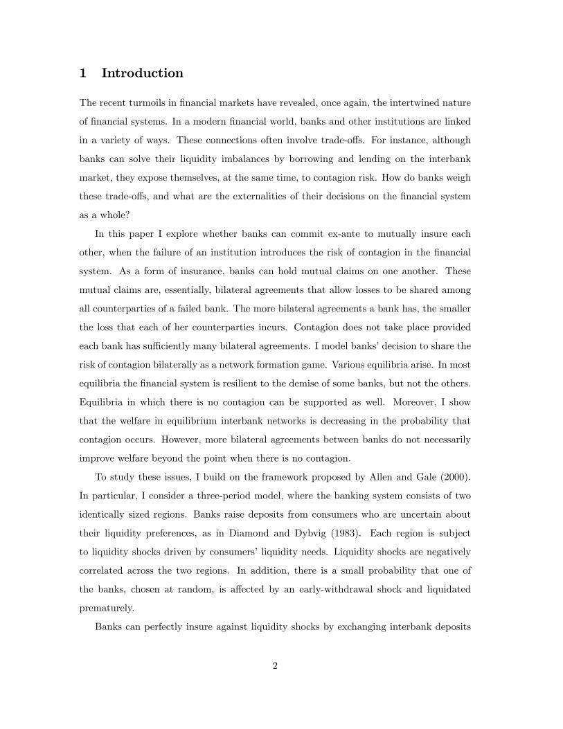
Table 1: Distribution of shocks in the economy at date 1

that value consumption at date 1 is q. However, each sector experiences fluctuations of

early withdrawals. With probability 1/2, in each sector there is either a high proportion,

pH , or a low proportion, pL, of early consumers, so that q = pH+pL2 . In particular, the

economy consists of two regions, A = {1, 2, ..., n} and B = {n+ 1, n+ 2, ..., 2n}, such that

fluctuations in the fraction of early consumers are perfectly correlated within each region

and negatively correlated across regions. That is, when sectors in region A receive a high

fraction, sectors in region B receive a low fraction, and the other way around.

Aggregate early-withdrawal shocks can affect the economy with a small, but positive,

probability ϕ. In this case, the average fraction of early consumers is higher than q.

For tractability, I assume that exactly one of the sectors receives a fraction (q + χ) of

early consumers, whereas the others receive a fraction q. Each sector is equally likely

to experience an early-withdrawal shock. The uncertainty in the liquidity preferences of

consumers at date 1 is summarized in Table 1.1

At date 0 each of the sectors is ex-ante identical. All the uncertainty is resolved at date

1, when the state of the world is realized and commonly known. At date 2, the fraction

of late consumers in each region will be (1 − p) where the value of p is known at date 1,

as either pH , pL, q or q + χ.

1Each realization of the aggregate early-withdawal shock in which sector k receives a fraction (q + χ)

of early consumers represents a state Sk that occurs with probability ϕ2n. I abuse notation and refer to the

set of states{Sk}kas state S that occurs with probability ϕ.

6

2.2 Banks, investment opportunities and interbank deposits

In each sector i there is a competitive representative bank. Agents deposit their endowment

in their sector’s bank. In exchange, they receive a deposit contract that promises a finite

amount of consumption depending on the date they choose to withdraw their deposits, and

that is, possibly, contingent on the state of the world. In particular, the deposit contract

specifies that if they withdraw at date 1, they receive CS1i ≥ 1, and if they withdraw at

date 2, they receive CS2i ≥ CS1i, where S ∈ {S1, S2, S}.

Banks have two investment opportunities: a liquid asset with a return of 1 after one

period, or an illiquid asset that pays a return of r < 1 after one period, or R > 1

after two periods. Let xi and yi be the per capita amounts that a bank i invests in the

liquid and illiquid asset, respectively. In addition, banks can deposit funds at other banks

in exchange for the same deposit contract offered to consumers. That is, for each unit

that bank i deposits at bank j, she is promised CS1j if withdrawing at t = 1 and CS2j if

withdrawing at time t = 2. Let zij denote the amount that bank i deposits at bank j, and

zi denote the total amount of interbank deposits that bank i holds.

Interbank deposits connect the banks in a network g. In particular, if bank i holds

deposits at bank j, they are considered to have a link ij and to be neighbors in the

network g. The set of neighbors of a bank i in the network g is Ni(g) = {j ∈ A ∪

B | ij ∈ g for any j 6= i}.

A set of contracts(CS1i, C

S2i

)i∈A∪B and portfolio allocations (xi, yi, zi)i∈A∪B is feasible

if it respects the feasibility constraints at date 0, 1, and 2, as follows.

At date 0, each bank i’s portfolio must satisfy the following feasibility constraint

xi + yi +∑

j∈Ni(g)zij = 1 +

∑j

i∈Nj(g)

zji.

In other words, the amount that a bank i receives from depositors, 1, and other banks,(∑j, i∈Nj(g) zji

), can be invested in the liquid asset, the illiquid asset, or as deposits at

other banks.

The feasibility constraint at date 1 requires that the payments to the early consumers

and to banks that withdraw at date 1 equal the cash inflows from the liquid asset and the

deposits withdrawn from other bank at date 1, in state S1 and S2. In state S1, banks

7

in region A withdraw deposits from banks in region A and B, whereas banks in region

B withdraw deposits only from other banks in region B. Similarly, in state S2, banks in

region B withdraw deposits from banks in region A and B, whereas banks in region A

withdraw deposits only from other banks in region A.

The feasibility constraint at date 2 requires that the payments to the late consumers

and to banks that withdraw at date 2 equals the cash inflows from the illiquid asset and

from the deposits withdrawn from other banks at date 2, in state S1 and S2. In state S1,

banks in region B withdraw deposits from banks in region A. Similarly, in state S2, banks

in region A withdraw deposits from banks in region B.

The feasibility constraints are, essentially, budget constraints. The condition that

contracts and portfolio allocations respect the feasibility constraints in states S1 and S2,

simply rules out that defaults occur in either of these states. However, I allow for the

possibility that defaults occur in state S, as banks are not required to have a balanced

budget in this state.

2.3 Interbank networks

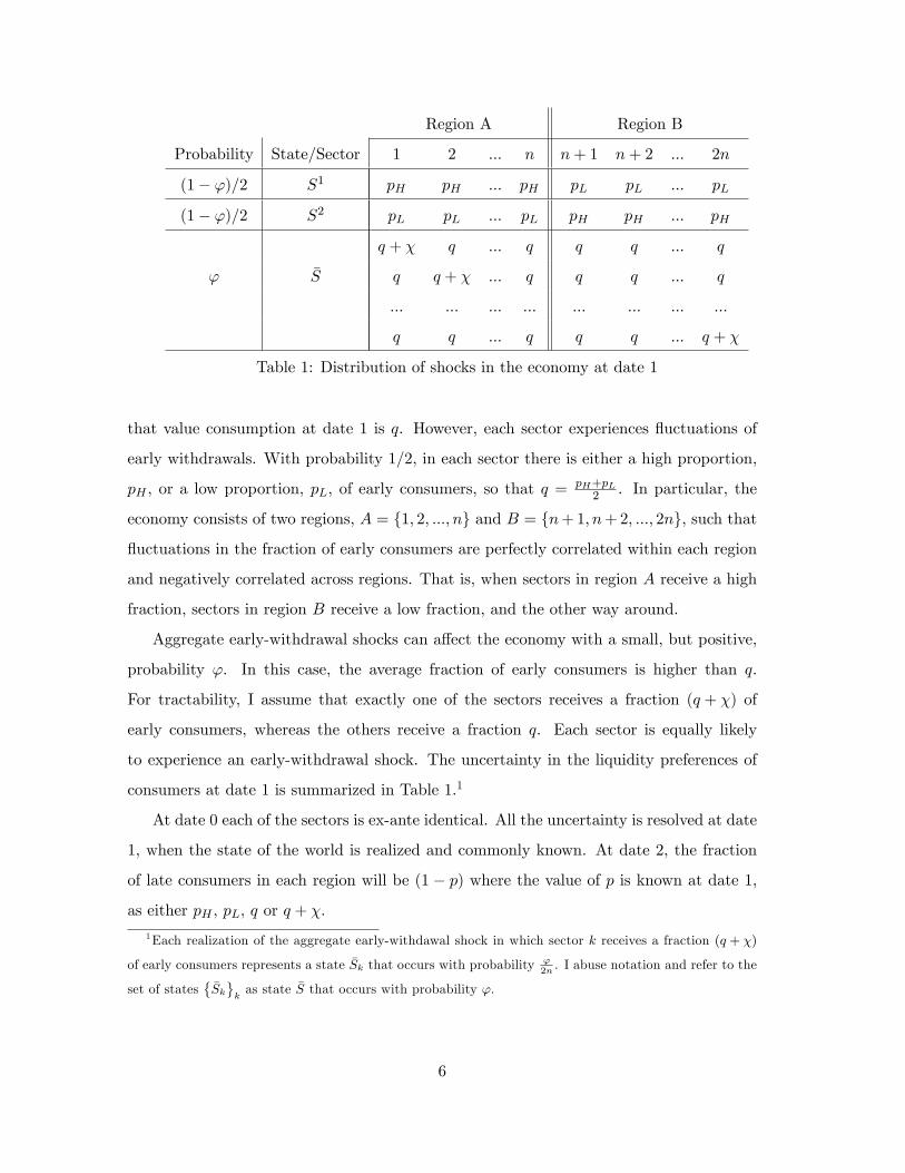
Various networks of interbank deposits can be considered. Figure 1 illustrates several

patterns of connections between banks. In a liquidity network each bank has connections

only with banks in the other region. In a symmetric network each bank has the same

number of links. A symmetric liquidity network is shown in Figure 1(a), and a symmetric

network is shown in Figure 1(b). Figure 1(c) represents a network in which each bank has

the same number of connections with banks in the other region, but a different number of

connections with banks in the same region. The links that banks have with other banks

in the same region represent a solvency network. In a complete network each banks has

connections with all other banks, as shown in Figure 1(d).

I will use the following notation throughout the paper. Let g`,ηi

represent networks

where each bank i has ` liquidity links with banks in the other region and ηi solvency links

with banks in the same region. If all banks have same the number, η, of connections with

banks in the same region, then the network is symmetric and denoted g`,η. For instance

gn,n represents the complete network, while gn,0 represents a symmetric liquidity network

in which each bank has links with all the bank in the other region, and no links with banks

8

A B 1

2

4

3

8

7

6

5

(a) (b)

(c) (d)

A B 1 5

6

7

2

3

4 8

A B 1 5

6

7

2

3

4 8

A B 1 5

6

7

2

3

4 8

Figure 1: This figure illustrates various patterns of connections between banks. Panel (a) shows a sym-

metric liquidity network. Panel (b) illustrates a symmetric interbank network. Panel (c) illustrates an

interbank network in which each bank has the same number of links with banks in the other region, but a

different number of links with banks in the same region. Panel (d) illustrates a complete network.

in the same region.

In the analysis in the following section I focus on the case in which each bank has `

connections with banks in the other region. The main results, aside of Proposition 5, are

derived for ` = n.

3 Interbank Contagion

3.1 Optimal risk-sharing without aggregate uncertainty

The optimal risk sharing problem is well understood if there is no aggregate uncertainty

about the average fraction of early consumers (i.e. when ϕ = 0). Allen and Gale (2000)

characterize the optimal risk sharing allocation as the solution to a planning problem.

They show that the optimal deposit contract (C∗1 , C∗2 ) is state-independent, and maximizes

the ex-ante expected utility of consumers. In the case when consumers have log-preferences

it follows straightforwardly that

(C∗1 , C∗2 ) = (1, R) . (1)

9

Moreover, the optimal portfolio allocation requires that each bank i invests an amount x∗

in the liquid asset in order to pay the early consumers and an amount y∗ = (1− x∗) in

the illiquid asset in order to pay the late consumers

(x∗, y∗) = (qC∗1 , (1− q)C∗2/R). (2)

As Allen and Gale (2000) show, an interbank system can decentralize the planner’s solu-

tion, if each bank deposits with banks in the other region a total amount z∗ = pH − q =

q − pL, at date 0.2

The planner’s solution can be implemented by any symmetric liquidity network, g`,0,

where each bank has liquidity links with ` ∈ {1, 2, ..., n} banks in the other region, and

the amount of deposits exchanged between any two banks is z∗

` at date 0. Moreover, any

network g`,ηi

in which any two banks that have a link exchange z∗

` as deposits at date

0 can also decentralize the planner solution. This is because deposits exchanged with

banks in the same region mutually cancel out in either state S1 or S2, as they do not

provide insurance against regional liquidity fluctuations. At the same time, although a

bank can deposit more than z∗ with banks in the other region, in an interbank network

g`,ηi

insurance against liquidity shocks can be achieved only if banks that have a liquidity

shortage withdraw a net amount of z∗

` from the banks that have a liquidity surplus.

It is straightforward to see that the contract (1) and the portfolio (2) respect the

feasibility constraints introduced in Section 2.2. Moreover, no defaults occur when ϕ = 0.

3.2 Defaults and the contagion mechanism

Next, I consider the case of ϕ > 0, when each bank incurs an early-withdrawal shock

with probability 1/2n in state S. I show that defaults and contagion can occur in a given

interbank network, g`,ηi, in which banks offer the deposit contract (1), hold the portfolio

(2), and insure an amount z∗/` as bilateral deposits with other banks. I assume that each

bank exchanges z∗/` deposits with both banks in the other region, as well as banks in the

2Exchanging interbank deposits ex-ante in order to insure against liquidity shocks may be seen as

uncoventional. Acharya et al. (2012) emphasize some of the problems that occurs when liquidity transfers

occur ex-post. For instance, surplus banks may strategically under-provide lending to induce ineffi cient

sales of assets from needy banks.

10

same region. Although it is feasible to consider that banks in the same region exchange

a different amount as deposits, this assumption simplifies our analysis without losing any

insights.

A bank that needs to repay (q + χ)C∗1 to the early consumers in state S does not have

suffi cient liquidity at date 1, as the proceeds from the liquid asset are x∗ = qC∗1 . Hence,

the bank must liquidate either some of its interbank deposits and/or the illiquid asset. As

in Allen and Gale (2000), I assume that the costliest in terms of early liquidation is the

illiquid asset, followed by interbank deposits:

C∗2C∗1

<R

r. (3)

This implies that the bank liquidates deposits in other regions before it liquidates the

illiquid asset. In state S, liquidating interbank deposits, although beneficial, as I describe

below, does not generate liquidity. Thus, the bank must liquidate at least part of the

illiquid asset in order to meet withdrawals from early consumers.

A bank that liquidates the illiquid asset prematurely, affects negatively the consump-

tion of late withdrawers. In fact, if too much of the illiquid asset is liquidated early, the

consumption of late consumers may be reduced to a level below C∗1 . In this case, the late

consumers gain more by imitating the early consumers and withdrawing their investment

from the bank at date 1. This induces a run on the bank. The maximum amount of

illiquid asset that can be liquidated without causing a run is given by

b ≡ y∗ − (1− q)C∗1R

, (4)

or, substituting from (2),

b = (1− q)(C∗2 − C∗1 )

R.

For the remainder of the paper, I assume that

χ >r · bC∗1

. (5)

In other words, the amount that can be obtained at date 1 by liquidating the long asset

without causing a run, r · b, is not suffi cient to repay the additional fraction, χ, of early

depositors. Thus, a bank which offers the deposit contract (1), and holds the portfolio (2)

cannot repay C∗1 to depositors that withdraw at date 1, if she incurs an early-withdrawal

11

shock in state S. In this case, the bank defaults, and its portfolio of assets is liquidated

at the current value and distributed equally among creditors.

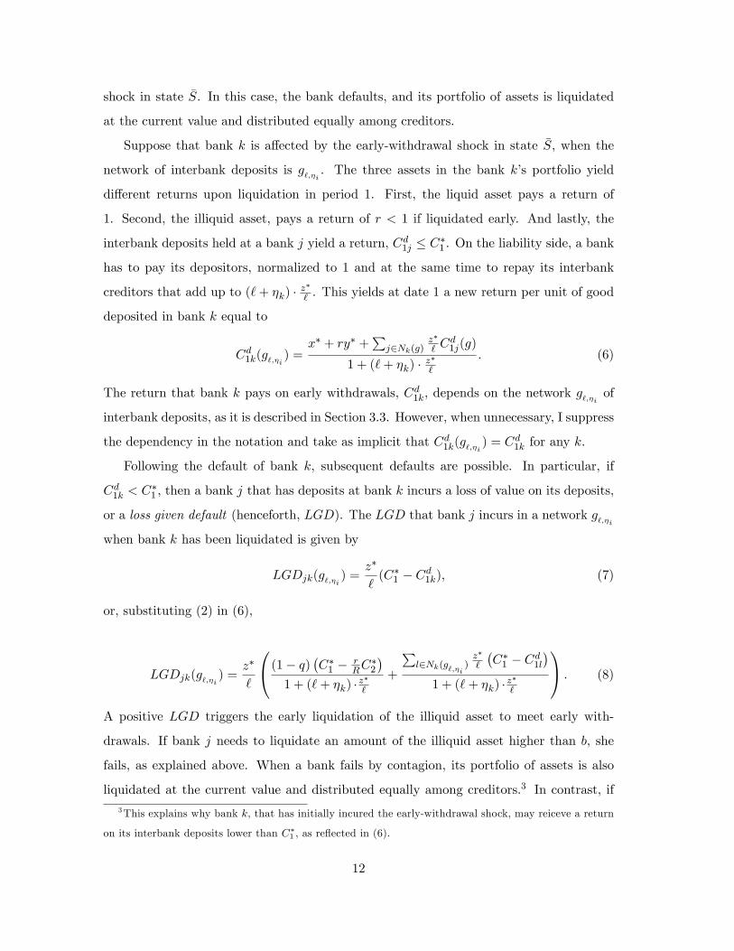
Suppose that bank k is affected by the early-withdrawal shock in state S, when the

network of interbank deposits is g`,ηi. The three assets in the bank k’s portfolio yield

different returns upon liquidation in period 1. First, the liquid asset pays a return of

1. Second, the illiquid asset, pays a return of r < 1 if liquidated early. And lastly, the

interbank deposits held at a bank j yield a return, Cd1j ≤ C∗1 . On the liability side, a bank

has to pay its depositors, normalized to 1 and at the same time to repay its interbank

creditors that add up to (`+ ηk) · z∗

` . This yields at date 1 a new return per unit of good

deposited in bank k equal to

Cd1k(g`,ηi ) =x∗ + ry∗ +

∑j∈Nk(g)

z∗

` Cd1j(g)

1 + (`+ ηk) · z∗`

. (6)

The return that bank k pays on early withdrawals, Cd1k, depends on the network g`,ηi of

interbank deposits, as it is described in Section 3.3. However, when unnecessary, I suppress

the dependency in the notation and take as implicit that Cd1k(g`,ηi ) = Cd1k for any k.

Following the default of bank k, subsequent defaults are possible. In particular, if

Cd1k < C∗1 , then a bank j that has deposits at bank k incurs a loss of value on its deposits,

or a loss given default (henceforth, LGD). The LGD that bank j incurs in a network g`,ηi

when bank k has been liquidated is given by

LGDjk(g`,ηi ) =z∗

`(C∗1 − Cd1k), (7)

or, substituting (2) in (6),

LGDjk(g`,ηi ) =z∗

`

(1− q)(C∗1 − r

RC∗2

)1 + (`+ ηk) · z

∗`

+

∑l∈Nk(g

`,ηi)z∗

`

(C∗1 − Cd1l

)1 + (`+ ηk) · z

∗`

. (8)

A positive LGD triggers the early liquidation of the illiquid asset to meet early with-

drawals. If bank j needs to liquidate an amount of the illiquid asset higher than b, she

fails, as explained above. When a bank fails by contagion, its portfolio of assets is also

liquidated at the current value and distributed equally among creditors.3 In contrast, if3This explains why bank k, that has initially incured the early-withdrawal shock, may reiceve a return

on its interbank deposits lower than C∗1 , as reflected in (6).

12

the amount of the illiquid asset liquidated at date 1 is below the threshold b, bank j does

not default and returns C∗1 for early withdrawals. Nevertheless, it will be costly for the

late consumers, as their consumption is now reduced to Cd2j < C∗2 . Thus, b given by (4)

represents a contagion threshold, as it is the maximum amount of illiquid asset that a bank

can liquidate without causing a run.

Two distinct implications follow from (8). First, the loss given default LGDjk is

increasing in the amount of deposits, z∗

` , exchanged between the two banks. In other

words, the more liquidity links, `, each bank has with banks in the other region, the

smaller is the loss given default. Second, the more links bank k has with banks that are

able to repay C∗1 for deposits, the smaller is the loss LGDjk it induces to a neighbor j. This

effect is independent of the amount of deposits exchanged between banks, and it arises,

for instance, when keeping the number of links, `, with banks in the other region constant

and increasing the number of solvency links, ηk, with banks in the same region. There

are two channels that explain this second implication. Everything else equal, increasing

the number of links with banks that are able to repay a return for deposits of C∗1 at date

1, mechanically decreases the loss that bank k induces to its neighbors. This is because,

the denominator in (8) increases, while the numerator remains the same. In other words,

the loss that bank k induces when it fails is redistributed across more counterparties. At

the same time, a positive spiral that further reduces the loss-given-default may arise. For

instance, the LGDjk incurred by neighbor j may decrease suffi ciently, such that bank j

does not default by contagion and is also able to repay bank k a return C∗1 per-unit of

deposits. Then, the loss that k induces to its neighbors decreases even further, reaching

its minimum when none of the neighbor banks defaults

LGDminjk (ηk) =

z∗

`

(1− q)(C∗1 − r

RC∗2

)1 + (`+ ηk)

z∗`

, (9)

for any j ∈ Nk(g`,ηi ).

Thus, the contract (1) and portfolio (2) involve a trade-off. Because defaults involve the

liquidation of the illiquid asset, there is a utility loss in state S. A different arrangement,

in which banks invest more in the liquid asset and insure less through the interbank system

may be desirable. A bank that has cash reserves, can avoid a run if it incurs an early-

withdrawal shock. At the same time, she holds fewer deposits with other banks in the

13

system and incurs a lower loss-given-default. This way, banks can avoid default in state

S, at the expense of providing a lower utility to consumers in states S1 and S2.

In the remainder of the section I discuss the payoffs that banks expect to receive in

each state of the world4, under the assumption that each bank offers the deposit contract

(1) and holds the portfolio (2). In section 4, I come back to this issue and show that banks

find it optimal to offer the deposit contract (1) and to hold the portfolio (2) provided ϕ is

suffi ciently small. For now, I start by describing the payoffs in state S.

3.3 Expected payoffs

Consider as before that in state S bank k is affected by the early-withdrawal shock, and

suppose that the number of connections that bank k has with banks is in the same region,

ηk, satisfies the following inequality

z∗

`

(1− q)(C∗1 − r

RC∗2

)1 + (`+ ηk)

z∗`

≤ r · b. (10)

The left hand side of the inequality represents the loss-given default that a neighbor of

bank k receives in a network g`,ηi, provided all k’s neighbor banks repay a return C∗1 for

the deposits they have received from bank k. At the same time, repaying C∗1 is indeed

consistent with the loss-given-default that a neighbor j of bank k receives in the network

g`,ηi, as the maximum amount of the illiquid asset that can be liquidated without causing

a run, b, is larger thanLGDmin

jk (g`,ηi

)

r . This implies that in the network g`,ηi

each bank

returns for early withdrawals C∗1 , except for bank k which returns

Cd1k (ηk) = C∗1 −(1− q)

(C∗1 − r

RC∗2

)1 + (`+ ηk)

z∗`

. (11)

Moreover, each of the [2n− (`+ ηk + 1)] banks that do not have a connection with bank

k returns C∗2 for late withdrawals. However, each of the (`+ ηk) banks that have a

connection with bank k must liquidate an amount ofLGDmin

jk (g`,ηi

)

r from the illiquid asset

and returns for late withdrawals

Cd2j (ηk) = C∗2 −z∗

`

Rr C∗1 − C∗2

1 + (`+ ηk)z∗`

, (12)

4Banks are perfectly competitive and make zero-profits. However, because banks maximize the expected

utility of consumers, I abuse terminology and use banks’payoffs to refer to banks’consumers payoffs.

14

for any j ∈ Nk(g`,ηi ), with Cd2j (ηk) ≥ C∗1 .

In contrast, if inequality (10) does not hold, then any neighbor of bank k defaults by

contagion. This is because even if all (`+ ηk) neighbors of bank k repay C∗1 , they still need

to liquidate too much of the illiquid asset. Clearly, this implies that it is impossible for

any of them to repay C∗1 to start with, and the realized loss-given-default is even higher.

When inequality (10) does not hold, the payoffs that banks receive depend on the

entire network structure. The procedure to finding the solution involves a sequence of

steps. First, find the return that bank k and each of its neighbors j ∈ Nk(g`,ηi ) repay

for early withdrawals. For this, solve the system of (`+ ηk + 1) equations implied by (6),

under the assumption that the remaining banks that are not neighbors of k do not default

and are able to repay C∗1 . Second, verify that these banks are indeed able to repay C∗1 ,

given the losses-given-default implied at the first step. If all banks that are not neighbors

of k are able to repay C∗1 , then the solution is the one found at the first step. Otherwise, if

a subset of m of these banks are not able to repay C∗1 , solve the system of (`+ ηk + 1 +m)

equations implied by (6), under the assumption that the remaining banks do not default

and are able to repay C∗1 . Verify that this is indeed consistent with the solution found.

Otherwise, continue the procedure until all banks default. This solutions concept is similar

to the algorithm that Elliott, Golub and Jackson (2013) propose to characterize waves of

defaults in a network of liabilities (which is a generalization of the algorithm in Eisenberg

and Noe, 2001).

Although a solution for a general network g`,ηi

is diffi cult to characterize, the following

proposition describes the payoffs that banks receive when ` = n, for any number of links

ηi that a bank i has with banks in the same region. Moreover, for the remainder of the

paper I assume as well that ` = n, and relax this assumption when I discuss incomplete

liquidity networks in Section 5.

15

Proposition 1 Consider any interbank network gn,ηi in which each bank offers the deposit

contract (1) and holds the portfolio (2). Let η be the smallest positive integer that satisfies

the inequalityz∗

n

(1− q)(C∗1 − r

RC∗2

)1 + (n+ η) z

∗n

≤ r · b. (13)

If the bank that is subject to the early-withdrawal shock in state S has less than η connec-

tions, then each bank returns per unit of deposit at date 1

Cd1 = C∗1 − (1− q)(C∗1 −

r

RC∗2

). (14)

The proof for Proposition 1 follows in two steps. First, I show that if the bank that

is subject to the early-withdrawal shock has less than η connections, then all the other

(2n−1) banks fail by contagion. Importantly, this is independent of how many connections

each bank has with banks in the same region, as the result holds for any network gn,ηi .

Second, I find the vector of returns(Cd1i)i∈A∪B that is a fixed point of the system of 2n

equations implied by (6).

Proposition 1 easily generalizes to any network g`,ηi

in which all banks default in state

S. In particular, let η(`) be the smallest integer for which inequality (10) holds. Consider

parameters such that if the bank subject to the early-withdrawal shock has less than η (`)

connections, then all the other (2n−1) banks fail by contagion. Then all banks return Cd1

per unit of deposit as given by (14).

At this stage I can characterize the payoffs that each bank i expects to receive in a

network gn,ηi . In both states S1 and S2, each bank has with probability half either a

high fraction, pH , of early consumers or a low fraction, pL, of early consumers. Hence,

consumers expect to receive in each of these states

qu (C∗1 ) + (1− q)u (C∗2 ) .

In state S, consumers’expected utility depends on how many banks have at least η connec-

tions with banks in the same region and on whether bank i, itself has at least η connections

with banks in the same region. Let H(gn,ηi ) ={j ∈ A ∪B|ηj ≥ η

}be the set of banks

that have at least η connections, and let h =∣∣H(gn,ηi )

∣∣ be the number of banks that haveat least at least η connections. This implies that there are (2n−h) banks that each induces

the default of the entire system, when affected by the early-withdrawal shock. Moreover,

16

let Hi(gn,ηi ) ={j ∈ Ni(gn,ηi )|ηj ≥ η

}be the set of neighbors of bank i that have at least

η connections. This implies that whenever a bank j ∈ Hi(gn,ηi ) is affected by the early-

withdrawal shock, bank i returns to its late consumers Cd2i(ηj)as given by (12) for ` = n.

In addition, the return that bank i pays in case it is affected by the early-withdrawal shock

depends on how many connections it has. Thus, if i ∈ H(gn,ηi ), then it returns Cd1i (ηi) as

given by (11) for ` = n. Otherwise, it returns Cd1 as given by (14).

The expected payoff of a given bank i is as follows

πi(gn,ηi ) = (1− ϕ) [q ln (C∗1 ) + (1− q) ln (C∗2 )] (15)

+ϕ

[2n− h

2nln(Cd1

)+

1

2n

∑j∈Hi(gn,ηi )

(q ln(C∗1 ) + (1− q) ln

(Cd2i(ηj)))

+1

2n

∑j∈H(gn,ηi )\Hi(gn,ηi )

(q ln(C∗1 ) + (1− q) ln (C∗2 ))

],

if i /∈ H(gn,ηi ), and

πi(gn,ηi ) = (1− ϕ) [q ln (C∗1 ) + (1− q) ln (C∗2 )] (16)

+ϕ

[2n− h

2nln(Cd1

)+

1

2n

∑j∈Hi(gn,ηi )

(q ln(C∗1 ) + (1− q) ln

(Cd2i(ηj)))

+1

2n

∑j∈H(gn,ηi )\Hi(gn,ηi )

(q ln(C∗1 ) + (1− q) ln (C∗2 ))

+1

2nln(Cd1i (ηi)

)],

if i ∈ H(gn,ηi ).

4 Endogenous Solvency Networks

When there is a risk of contagion in the financial system, banks can take actions to insure

against it. The decisions that each bank i must consider at date 0 in order to maximize

the expected utility of consumers, consist of a deposit contract (CS1i, CS2i) for early and late

withdrawals, a portfolio of liquid and illiquid assets and interbank deposits (xi, yi, z∗i ), a set

of liquidity links with banks in the other region, and a set of solvency links with banks in

the same region. In particular, consider the following timing of events at date 0. At stage

1, each bank chooses a deposit contract and a portfolio allocation. At stage 2, each bank

chooses a set of links with banks in the other region, specifying for each link the amount

of interbank deposits she wants to insure with the respective counterparty. At stage 3,

17

each bank chooses a set of links with banks in the same region, specifying as well, for each

link, the amount of interbank deposits it wants to insure with the respective counterparty.

At each stage, each bank takes the decisions at previous stage(s), as well, the decisions

of other at the current stage as given. Furthermore, at each stage banks understand the

consequences of their current decisions on the choices to be made at future stage(s). In

making choices, at each stage banks could reason backwards and choose the deposit the

contract that maximizes the expected utility of consumers.

The diffi culty with this approach is that decisions at stage 2 (and 3) involve both a set

of links, as well as an amount of deposits for each link. This prevents agents from taking

decisions unilaterally, or even bilaterally. For instance, consider a symmetric liquidity

network g`,0where each bank has ` links with banks in the other region, and any two

banks that have a link exchange an amount z∗

` as deposits. Suppose that at stage 1,

banks offer the deposit contract (C∗1 , C∗2 ), hold the portfolio (x∗, y∗) and insure an amount

z∗ = (pH − q) as interbank deposits. Then, a bank that is considering decreasing the

number of links with banks in the other region from ` to `− 1, must re-adjust the amount

of deposits it exchanges with at least one other bank (from z∗

` to2z∗

` ), in order to respect

the feasibility constraints described in Section 2.2. However, the re-adjustment cannot

be done unilaterally as her counterparty has an excess of incoming deposits, unless she

re-adjusts the deposits she exchanges with other counterparties in order to respect her

feasibility constraints.

The approach I take instead is similar to the solution method in Dasgupta (2004).

First, I analyze the equilibrium networks on the continuation path induced by the deposit

contract (1) and the portfolio (2), when each bank has n connections with banks in the

other region and any two banks that have a link exchange z∗

n in deposits. Second, I show

that each bank’s best response is to offer the deposit contract (1) and the portfolio (2)

when all other banks offer the deposit contract (1) and the portfolio (2), at least when the

probability of state S is suffi ciently small.5

5A complimetary approach is to consider that banks first choose a set of links and then choose a deposit

contract and a portfolio allocation. Acemoglu et al. (2015) explore this route using a solution strategy

similar to mine. In particular, they solve for the equilibrium interbank lending decisions and interest rates,

given that banks are connected in an exogenous network which restricts the amount they can borrow from

18

To analyze the equilibrium networks, I model the interaction between banks in the

same region as a game in which banks choose with whom to form links. Such a game is

called a network formation game. The formation of a link requires the consent of both

parties involved, since banks mutually exchange deposits. However, the severance of a

link can be done unilaterally, as deposits can be withdrawn on demand by either of the

banks involved in a link (in this case, deposits will be restituted to both banks, although

only one party exercises the claim). To identify equilibrium networks, I use the concept

of pairwise stability introduced by Jackson and Wolinsky (1996).6

Definition 1 An interbank network g is pairwise stable if

(i) for any pair of banks i and j that are linked in the interbank network g, neither of

them has an incentive to unilaterally sever their link ij. That is, the expected profit each

of them receives from deviating to the interbank network (g − ij) is not larger than the

expected profit that each of them obtains in the interbank network g (πi(g − ij) ≤ πi(g)

and πj(g − ij) ≤ πj(g));

(ii) for any two banks i and j that are not linked in the interbank network g, at least

one of them has no incentive to form the link ij. That is, the expected profit that at least

one of them receives from deviating to the interbank network (g + ij) is not larger than

the expected profit that it obtains in the interbank network g (if πi(g + ij) > πi(g) then

πj(g + ij) < πj(g)).

The result below describes whether forming or severing links is profitable for any given

pair of banks i and j, depending on the number of links that they have in a network gn,ηi .

The derivations are shown in Appendix B.

Proposition 2 The marginal payoffs of forming and severing a link, respectively, for bank

i in a network gn,ηi are characterized by the following properties:

each other. They study then whether equilibrium outcomes are optimal or not, depending on the network

structure.6This concept has been applied by Zawadowski (2013) to analyze the stability of bilateral insurance

contracts in the context of OTC markets. More recently, Farboodi (2014) uses an extension of the concept

that allows for group deviations to explain intermediation in interbank markets.

19

Property 1: πi(gn,ηi + ij) < πi(gn,ηi ) if ηi ≥ η or ηi ≤ η − 2 for any ηj ≥ η.

Property 2: πi(gn,ηi − ij) > πi(gn,ηi ) if ηi ≥ η + 1 or ηi ≤ η − 1 for any ηj ≥ η + 1.

Property 3: πi(gn,ηi + ij) > πi(gn,ηi ) if ηi ≥ η − 1 for any ηj ≤ η − 1, or for any ηi if

ηj = η − 1.

Property 4: πi(gn,ηi − ij) < πi(gn,ηi ) if ηi ≥ η for any ηj ≤ η, or for any ηi if ηj = η.

Property 5: πi(gn,ηi + ij) < πi(gn,ηi ), if ηi = η − 1 and ηj ≥ η, for any

r < z∗(n+η)n((2z∗+1)(n+η)−1) .

Property 6: πi(gn,ηi − ij) > πi(gn,ηi ), if ηi = η and ηj ≥ η + 1, for any

r < z∗(n+η)n((2z∗+1)(n+η)−1) .

Property 7: πi(gn,ηi + ij) = πi(gn,ηi ) if ηi ≤ η − 2 and ηj ≤ η − 2.

Property 8: πi(gn,ηi − ij) = πi(gn,ηi ) if ηi ≤ η − 1 and ηj ≤ η − 1.

The main trade-offs that banks take into account when forming or severing links are

as follows. On the one hand, there is an implicit cost of having a link with a bank that

has at least (η + 1) links (or forming a link with a bank that has η links). If she incurs

an early-withdrawals shock, her neighbors, though they do not default, are not able to

return C∗2 to the late consumers. This effect is captured by Properties 1−2. On the other

hand, banks are willing to sacrifice some utility from the late consumers if they can avoid

defaulting by contagion. Thus, banks find it beneficial to maintain a link with a bank that

has η links (or form a link with a bank that has (η − 1) links). This effect is captured by

Properties 3− 4.

The trade-off between the cost and benefit of linking is more complex in two cases,

which are characterized by Properties 5 − 6. When bank i has ηi = η − 1 links, forming

a new a link with a bank j that has ηj ≥ η links implies that bank i is able to repay

Cd1i(ηi + 1), as opposed to Cd1 , if she is affected by the early-withdrawal shock. However,

bank i can return only Cd2i(ηj + 1) for late withdrawals, as opposed to C∗2 , if bank j is

affected by the early-withdrawal shock. Similarly, when bank i has ηi = η links, severing

a a link with a bank j that has ηj ≥ η + 1 links implies that bank i returns only Cd1 , as

opposed to Cd1i(ηi), if she is affected by the early-withdrawal shock. However, bank i is

20

able to return C∗2 for late withdrawals, as opposed to Cd2i(ηj), if bank j is affected by the

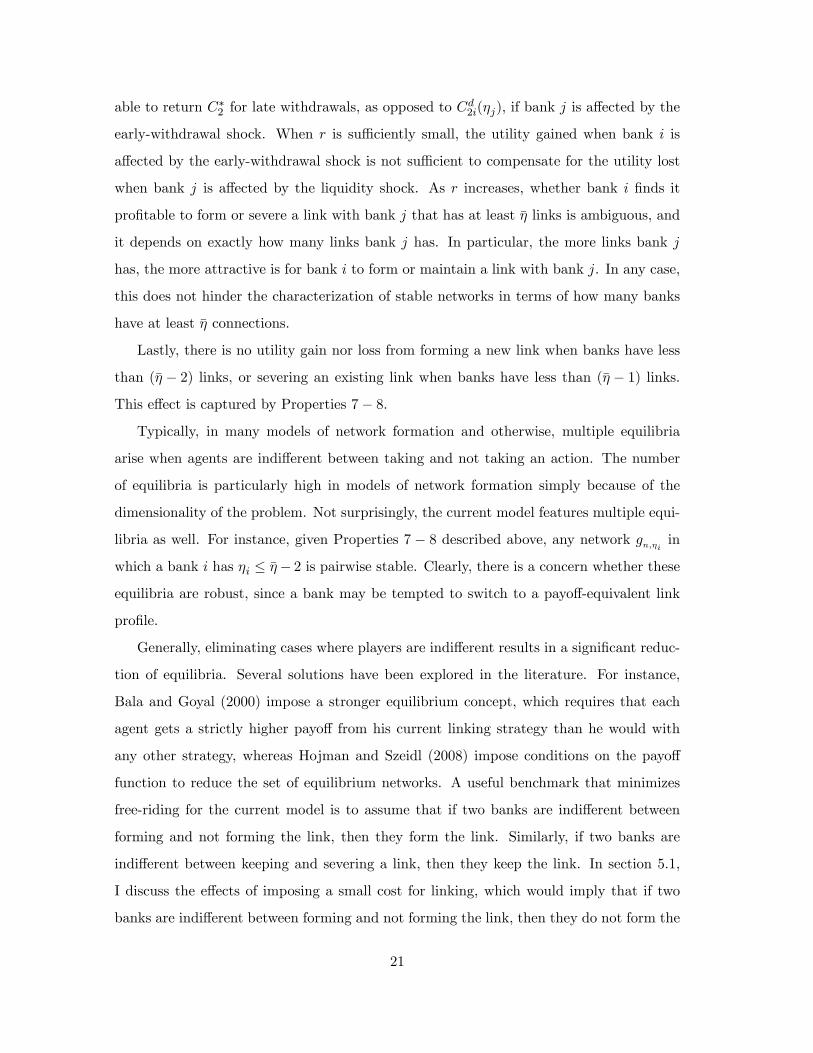
early-withdrawal shock. When r is suffi ciently small, the utility gained when bank i is

affected by the early-withdrawal shock is not suffi cient to compensate for the utility lost

when bank j is affected by the liquidity shock. As r increases, whether bank i finds it

profitable to form or severe a link with bank j that has at least η links is ambiguous, and

it depends on exactly how many links bank j has. In particular, the more links bank j

has, the more attractive is for bank i to form or maintain a link with bank j. In any case,

this does not hinder the characterization of stable networks in terms of how many banks

have at least η connections.

Lastly, there is no utility gain nor loss from forming a new link when banks have less

than (η − 2) links, or severing an existing link when banks have less than (η − 1) links.

This effect is captured by Properties 7− 8.

Typically, in many models of network formation and otherwise, multiple equilibria

arise when agents are indifferent between taking and not taking an action. The number

of equilibria is particularly high in models of network formation simply because of the

dimensionality of the problem. Not surprisingly, the current model features multiple equi-

libria as well. For instance, given Properties 7 − 8 described above, any network gn,ηi in

which a bank i has ηi ≤ η− 2 is pairwise stable. Clearly, there is a concern whether these

equilibria are robust, since a bank may be tempted to switch to a payoff-equivalent link

profile.

Generally, eliminating cases where players are indifferent results in a significant reduc-

tion of equilibria. Several solutions have been explored in the literature. For instance,

Bala and Goyal (2000) impose a stronger equilibrium concept, which requires that each

agent gets a strictly higher payoff from his current linking strategy than he would with

any other strategy, whereas Hojman and Szeidl (2008) impose conditions on the payoff

function to reduce the set of equilibrium networks. A useful benchmark that minimizes

free-riding for the current model is to assume that if two banks are indifferent between

forming and not forming the link, then they form the link. Similarly, if two banks are

indifferent between keeping and severing a link, then they keep the link. In section 5.1,

I discuss the effects of imposing a small cost for linking, which would imply that if two

banks are indifferent between forming and not forming the link, then they do not form the

21

link, whereas if two banks are indifferent between keeping and severing a link, then they

severe the link.

Properties 1 to 8 characterize the benefits and the costs of forming or severing links

for any given pair of banks i and j, spanning all combinations of the number of links that

they have in a network gn,ηi . For instance, consider the case of bank i, with ηi = η + 1,

and j, with ηj = η−2, that do not have a link. Property 3 characterizes the incentives for

bank i to form the link, while Property 1 characterizes the incentives for bank j to form

the link. These properties are useful in deriving the following result.

Proposition 3 Let gn,ηi be a pairwise stable network. Then there are at least max{2 (n− η) , n}

banks that have η connections with banks in the same region.

The main intuition for this result is as follows. The threshold number of connections

η determines what externality each bank has on the entire banking system. When a bank

that is affected by the early-withdrawal shock has less than η connections with banks in

the same region, all banks default by contagion as Proposition 1 shows. However, if a bank

that is affected by the early-withdrawal shock has at least η connections with banks in the

same region, then only the consumption of the late consumers of her neighbors is negatively

affected. These two types of externalities drive banks’incentives to form or severe links.

In particular, banks weigh the benefit of forming links that allow them to avoid defaulting

by contagion, against the implicit cost that late consumers incur. Properties 3− 4 imply

that banks are willing to incur the implicit cost for the late consumers, if they can avoid

default. However, they are better off if they free-ride on others’links.

The trade-off that a link involves is best illustrated by the following case. Consider

two banks, i with ηi = η − 1, and j with ηj ≥ η, that do not have a link. It follows from

Property 3 that bank j benefits from forming with i, as she exchanges a situation when

the failure of i induces its own failure, for a situation when the failure of i results in a

lower utility for her late consumers. However, bank i does not internalize the effects that

its own failure on other banks. That is, the utility gained when bank i is affected by the

early-withdrawal shock is not suffi cient to compensate for the utility lost when bank j is

affected by the liquidity shock, if r is not too large. In consequence, the link between i

and j is not formed, as the formation of a link requires the consent of both banks.

22

However, the result described in Proposition 3 does not depend on r being small

enough. This is because the trade-off described above generalizes to most pairs of banks.

In particular, Properties 3− 4 and 7− 8 imply that only banks that have less than η − 1

links unequivocally benefit from forming or maintaining links with each other. Thus, a

bank that has less than η − 1 links seeks to form links with other banks, until she has

at least η links and no other banks accepts a link with her, or until the only banks with

whom she does not have a link have at least η links. In consequence, there is always a set

of banks that have at least η links.

Proposition 3 has significant implications for the stability of the banking system. In

particular, when η is small, in equilibrium most of the banks have suffi cient links to prevent

a shock in one of the institutions spreading through contagion. From (13) it follows that

the higher r or R is, the smaller is η. However, even as η increases, in a stable network,

at least half the banks will have a suffi ciently many links such that the losses they may

generate are small enough.

The following result characterizes the probability of systemic risk in an equilibrium

interbank network.

Corollary 1 (i) Let gn,ηi be a pairwise stable network. Then the probability that all

banks default is at most min{ϕηn ,ϕ2 }.

(ii) There exist pairwise stable networks in which all banks have η links and the probability

that all banks default is 0.

This result identifies an upper bound on the probability that all banks default by

contagion in state S. Corollary 1 is an immediate consequence of Proposition 3, and a

proof is omitted. In a network gn,ηi all banks default by contagion when a bank that

has less η links with banks in the same region is affected by the early-withdrawal shock.

The result follows since there are at most min{2η, n}, and each banks is affected by an

early-withdrawal shock with probability 1/n.

Proposition 3 identifies many interbank networks that can be pairwise stable. The

following result refines the characterization, and, more importantly, provides a ranking of

equilibria based on their implied expected welfare.

23

Proposition 4 Let r < z∗(n+η)n((2z∗+1)(n+η)−1) . Then, in any pairwise stable network each

bank has at most η links. Moreover, the expected welfare in pairwise stable networks is

increasing in the number of banks that have η links.

While contagion can occur in any pairwise stable interbank network in which at least

one bank has less than η links, the probability that all banks default decreases with the

number of banks that have η links. The result follows as the welfare loss induced when a

bank that has less than η links is affected by the early-withdrawal shock is smaller then

the welfare loss when a bank that has η links is affected by the early-withdrawal shock.

Moreover, an interbank network in which all banks have η links and contagion never arises

can be supported as an equilibrium.7 Such interbank network insures the highest welfare

of all pairwise stable networks.

Up to now, I have analyzed equilibrium networks on the continuation path induced

by the deposit contract (1) and the portfolio (2). Clearly it is important to insure that

banks find it optimal to offer the deposit contract (1), and to hold the portfolio (2). The

following proposition shows that this is the case, at least if the probability of state S is

suffi ciently small.

Proposition 5 There exists ϕ ∈ (0, 1) such that there is an equilibrium in which each

bank offers the deposit contract (1) and holds the portfolio (2), for any ϕ ≤ ϕ.

Rather than deriving the equilibrium deposit contract and portfolio allocation that

maximizes the expected utility of consumers for each ϕ, Proposition 5 shows that each

bank’s best response is to offer the deposit contract (1) and the portfolio (2) when all

other banks offer the deposit contract (1) and the portfolio (2) if ϕ is suffi ciently small.

The intuition is as follows. Because the deposit contract (1) and the portfolio (2) is

optimal when ϕ = 0, a bank that invests more in the liquid asset provides a lower utility

to her consumers in state S1 and S2. In Lemma 1 in the appendix, I show that a bank

that deviates from the contract (1) and the portfolio (2), while all other banks continue

to choose the contract (1) and the portfolio (2), must be self-suffi cient. That is, the bank

7The existence of such an equilibrium network is conditional on whether symmetric networks in which

each banks has a total of n+ η links exist. Lovasz (1979) discusses in detail conditions for the existence of

a symmetric networks with 2n nodes, in which each node has n+ η links.

24

that deviates does not hold any interbank deposits. The lemma follows from the feasibility

conditions introduced in Section 2.2. In other words, the lemma relies on the assumption

that there are no defaults, and that a bank delivers at date 1 and 2 the deposit contract she

had promised at date 0, in states S1 and S2. Given this, I show that there is no pattern of

interbank deposits such that a bank that deviates from the contract (1) and the portfolio

(2) exchanges positive amounts with other banks in the system. Otherwise, there must be

at least another bank that defaults on the contract (1), either in state S1 or S2. Therefore,

the bank that deviates must offer a deposit contract for early and late withdrawals, and

hold a portfolio as when she is in autarky. This implies that the expected utility loss in

states S1 and S2 for the bank that deviates is strictly positive. Thus, even though the

bank may obtain a lower utility in state S when she offers the contract (1) and holds the

portfolio (2) than when she deviates, the deviation is sub-optimal if the probability of the

aggregate shock is suffi ciently small.

Proposition 5 formalizes the reasoning outlined in Allen and Gale (2000). Although

they do not explicitly write down the feasibility constraints at date 1 and 2, they argue

that in order to avoid default, a bank has to make a large deviation, rather than a small

one. The distortion this causes in the other states will not be worth it, if the probability

of the aggregate shock is suffi ciently small.

This result is indeed consistent with the numerical findings in Dasgupta (2004), who

illustrates that it is optimal for banks to fully insure against regional liquidity shocks, as

long as the probability of contagion is small.

5 Discussion

5.1 The model with linking costs

As described in Section 4, there is an implicit cost associated to forming links. In particu-

lar, a bank i must consider the utility loss for her late consumers that can potentially arise

when forming a link with a bank j that has ηj ≥ η links. This implicit cost introduces

a natural trade-off against the benefits that a link can bring. However, there is no cost

associated to forming a link with a bank that has less than η links. In fact, as Properties

7−8 imply, there are many cases in which banks are indifferent between forming or sever-

25

ing links. In the previous section I assumed that when two banks are indifferent between

forming and not forming the link, then they form the link, and when they are indifferent

between keeping and severing a link, then they keep the link. However, it is interesting to

understand what is the effect of introducing a small linking cost.

In this section I analyze the equilibrium interbank networks that arise when each bank

incurs a linking cost, ε. Because links with banks that have at least η links are inherently

costly, I am interested in the case when the cost of linking only marginally breaks the

indifference in banks payoffs implied by Properties 7− 8. In other words, I consider that

the linking cost is suffi ciently small that the ordering of payoffs described in Properties

1− 6 does not change. However, if two banks i, with ηi ≤ η − 2, and j, with ηj ≤ η − 2,

do not have a link in the network, they chose not to form a link. Similarly, if two banks

i, with ηi ≤ η − 1, and j, with ηj ≤ η − 1, have a link in the network, they chose not to

severe the link.

The existence of a cost of linking, ε, increases the set of pairwise stable interbank

networks. For instance, a network in which banks have no links with other banks in the

same region is pairwise stable. At the same time, a network in which all banks have η

links is also pairwise stable. In fact, the number of banks that have at least η links with

banks in the same region in a pairwise stable network can vary from zero to 2n. Similarly,

the probability that all banks default in state S ranges from 0 to ϕ.

Although in the presence of small linking costs it is not possible to provide an upper

bound for the probability that all banks default, I can nevertheless provide a ranking of

equilibria depending on their implied expected welfare. The result is similar to the one

derived in Section 4.

Proposition 6 Let r < z∗(n+η)n((2z∗+1)(n+η)−1) . Then, there exists ε such that for any linking

cost ε < ε, the expected welfare in pairwise stable networks is increasing in the number of

banks that have η links.

It is interesting to compare the outcomes in the case when there is a small linking cost

with the outcomes in the model in which banks favor linking, analyzed in the previous

section. In both cases, the pairwise network that yields the highest welfare is a network

in which all banks have η links. However, when links are costly there is no lower bound

26

on the number of banks that have at least η links. In contrast, in the model in which

banks favor linking there are at least max{2 (n− η) , n} banks that have at least η links.

As welfare is monotonic in both cases, this implies that the welfare in many equilibria in

the model with linking costs is lower than the minimum welfare that can be supported in

an equilibrium of the model in which banks favor linking.

This is interesting from a policy perspective as well. It appears that small transaction

costs are detrimental to financial stability. Indeed, not only that there are more equilibria

when links are costly, but there is also a higher risk that all banks default by contagion in

the additional equilibria.

5.2 Welfare in interbank networks

The intuition developed in Allen and Gale (2000) is that complete networks are more

resilient to contagion relative to incomplete networks. Inequality (13) shows indeed that

if each bank has at least η links with banks in the same region there is no contagion in an

interbank network. In fact, in any network in which all banks have at least η links there

is no contagion in state S. However, it is not necessarily the case that a network in which

banks have more than η links improves consumers’welfare.

To understand how consumers’welfare depends on the number of links that each bank

has with banks in the same region, I compare symmetric networks, gn,η , in which each

bank has (n+ η) links, for η ∈ {η, η + 1, ..., n− 1}. As for any η ≥ η there is no contagion

in an interbank network gn,η , then in state S one bank is affected by the early-withdrawal

shock, (n+ η) banks repay C∗1 to early consumers, but less than C∗2 to late consumers, and

(2n− (n+ η + 1)) banks are able to repay (C∗1 , C∗2 ) to depositors. Using(11) and (12), I

obtain the expected welfare of consumers in state S as

W S(gn,η)

= (2n− (n+ η + 1))× (q ln(C∗1 ) + (1− q) ln (C∗2 ))

+ (n+ η)×(q ln(C∗1 ) + (1− q) ln

(C∗2 −

z∗

n

Rr C∗1 − C∗2

1 + (n+ η) z∗n

))

+ ln

(C∗1 −

(1− q)(C∗1 − r

RC∗2

)1 + (n+ η) z

∗n

).

Two opposite effects are transparent from this expression. On the one hand, the consumers

of the bank that is affected by the early-withdrawal shock and of her neighbors benefit

27

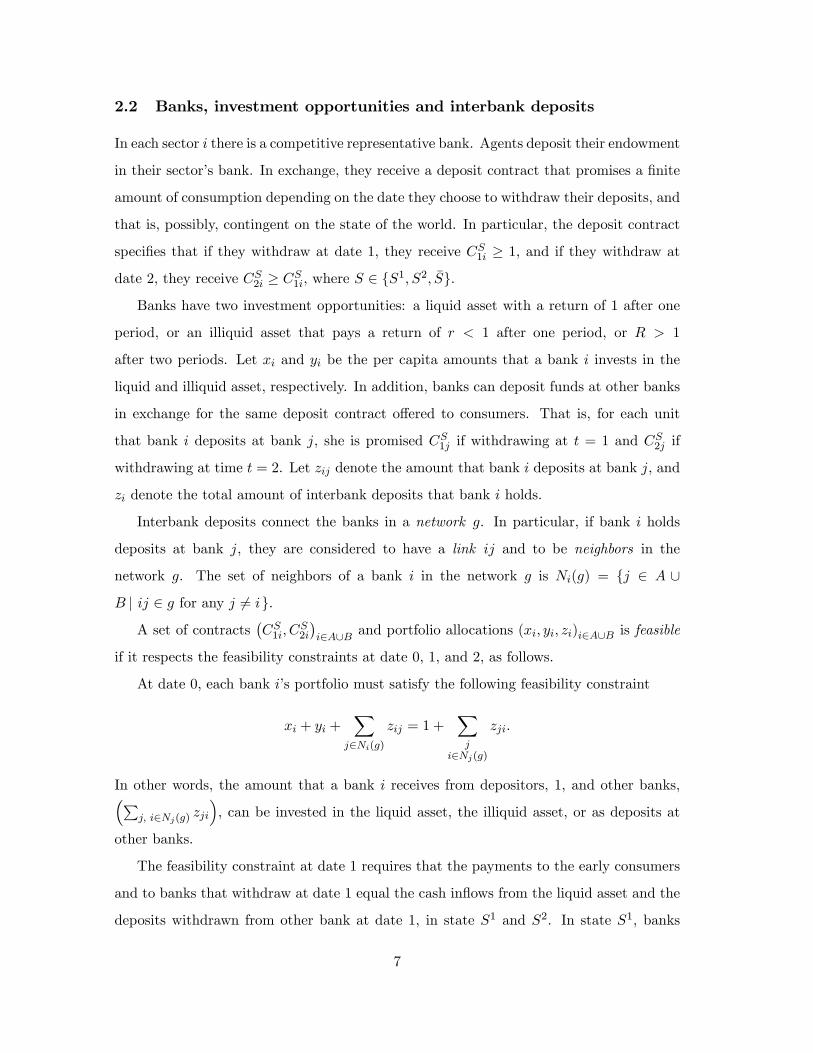
Figure 2: The figures depicts the expected welfare for an interbank network with 2n = 20 banks in which

contagion does not occur if each bank has at least η = 5 links, as the number of link that each bank

increases from 5 to n − 1 = 9. The parameters for this plot are as follows: R = 2, r = 0.03, pH = 0.6,

pL = 0.2. Consumers are assumed to have log-preferences.

as η increases. On the other hand, the number of banks that are able to repay (C∗1 , C∗2 )

to their depositors decreases, as η increases. Figure 2 illustrates that the second effects

can dominate. In particular, the figures shows that the welfare for an interbank network

with 2n = 20 banks in which contagion does not occur if each bank has at least η = 5

links decreases as the number of link that each bank increases from 5 to n − 1 = 9.

Thus, equilibrium networks in which contagion does not occur can also have the highest

associated welfare.

5.3 Incomplete liquidity networks, or ` < n

The main analysis of equilibrium solvency networks is under the assumption that the

liquidity network is complete. That is, each bank has links with all other banks in the

other region (` = n, ∀ i ∈ N). It would be interesting to understand however what effects

arise when the liquidity network is incomplete, or when ` < n.

Consider η(`) be the smallest integer for which inequality (10). Then, there are two

possibilities when ` < n. First, let ` be such that all banks default by contagion if the

bank that is subject to the early-withdrawal shock has less than η (`) connections, for

28

(a) (b)

A B1 5

6

7

2

3

4 8

A B1 5

6

7

2

3

4 8

Figure 3: This figures illustrates two possible patterns of connection between banks, when each bank has

` = 2 liquidity links with banks in the other region. Panel (a) illustrates a network with two disconnected

components. Panel (b) illustrates a connected interbank network, in which from each bank there is a path

of links to any other bank.

any pattern of links between banks or number of links with banks in the same region. In

this case, the result in Proposition 1 holds and all banks return Cd1 per unit of deposit

as given by (14). Then, properties 1− 8 described in Section 4 still characterize, at least

qualitatively, the payoffs for forming or severing links with banks in the same region. In

these conditions, it is possible to establish a lower bound on the number of banks that

have η(`) links similar to the one in Proposition 3.

Second, consider the case when ` is such that not all banks default by contagion if

the bank that is subject to the early-withdrawal shock has less than η (`) connections. A

stark example is given by the case of a banking system with eight banks in which each

banks has ` = 2 links with banks in the other region and no links with banks in the same

region. Suppose that η(2) = 1. In Figure 3(a), the interbank network is disconnected in

two separate components. Then, only four banks default when a bank is affected by an

early-withdrawal shock. In contrast, in Figure 3(b), the interbank network is connected

as from each bank there is a path of links to any other bank in the interbank network.

Then, when a bank is affected by the early-withdrawal shock, her two immediate neighbors

default, then her neighbors’neighbors default, with all banks defaulting at the end.8

As explained in Section 4, the payoffs that banks receive in the general case when

8Connectedness is not a suffi cient condition for all banks to default. One can construct more intricate

examples of connected networks in which the first wave of defaults is contained. For instance, suppose

that the neighbors of a bank affected by the idiosyncratic shock are well linked. Then, even if they default,

their neighbors can act as a buffer so contagion does not spread.

29

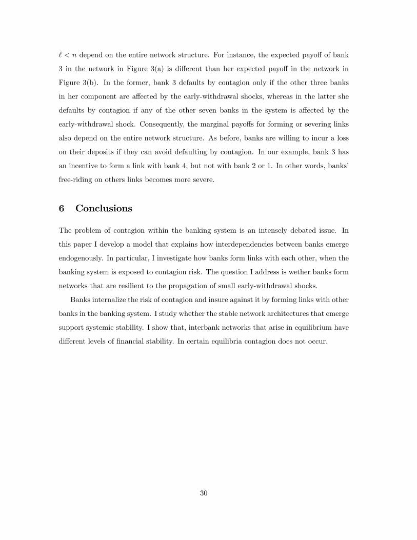
` < n depend on the entire network structure. For instance, the expected payoff of bank

3 in the network in Figure 3(a) is different than her expected payoff in the network in

Figure 3(b). In the former, bank 3 defaults by contagion only if the other three banks

in her component are affected by the early-withdrawal shocks, whereas in the latter she

defaults by contagion if any of the other seven banks in the system is affected by the

early-withdrawal shock. Consequently, the marginal payoffs for forming or severing links

also depend on the entire network structure. As before, banks are willing to incur a loss

on their deposits if they can avoid defaulting by contagion. In our example, bank 3 has

an incentive to form a link with bank 4, but not with bank 2 or 1. In other words, banks’

free-riding on others links becomes more severe.

6 Conclusions

The problem of contagion within the banking system is an intensely debated issue. In

this paper I develop a model that explains how interdependencies between banks emerge

endogenously. In particular, I investigate how banks form links with each other, when the

banking system is exposed to contagion risk. The question I address is wether banks form

networks that are resilient to the propagation of small early-withdrawal shocks.

Banks internalize the risk of contagion and insure against it by forming links with other

banks in the banking system. I study whether the stable network architectures that emerge

support systemic stability. I show that, interbank networks that arise in equilibrium have

different levels of financial stability. In certain equilibria contagion does not occur.

30

References

Acemoglu, D., A. Ozdaglar, and A. Tahbaz-Salehi, 2013, Systemic Risk and Stability in

Financial Networks, NBER Working Paper No. 18727.

Acharya, V., D. Gromb, and T. Yorulmazer, 2012, Imperfect Competition in the Interbank

Market for Liquidity as a Rationale for Central Banking, American Economic Journal:

Macroeconomics 4, 184—217.

Allen, F., and D. Gale, 2000, Financial Contagion, Journal of Political Economy 108,

1—33.

Alvarez, F., and G. Barlevy, 2014, Mandatory disclosure and financial contagion, Federal

Reseve Bank of Chicago Working Paper 2014 - 04.

Bala, V., and S. Goyal, 2000, A Non-Cooperative Model of Network Formation, Econo-

metrica 68, 1181—1230.

Caballero, R., and A. Simsek, 2012, Fire Sales in a Model of Complexity, Journal of

Finance forthcoming.

Castiglionesi, F., and N. Navarro, 2007, Optimal Fragile Financial Networks, mimeo,

Tilburg University.

Corbae, D., and J. Duffy, 2008, Experiments with Network Formation, Games and Eco-

nomic Behavior 64, 81—120.

Dasgupta, A., 2004, Financial Contagion Through Capital Connections: A Model of the

Origin and Spread of Bank Panics, Journal of European Economic Association 2, 1049—

1084.

Diamond, D., and P. Dybvig, 1983, Bank Runs, Deposit Insurance and Liquidity, Journal

of Political Economy 91, 401—419.

Duffi e, D., and H. Zhu, 2011, Does a Central Clearing Counterparty Reduce Counterparty

Risk?, Review of Asset Pricing Studies 1, 74—95.

31

Eisenberg, L., and T. Noe, 2001, Systemic Risk in Financial Systems,Management Science

47, 236—249.

Elliott, M., B. Golub, and M. Jackson, 2013, Financial Networks and Contagion, working

paper Stanford University.

Farboodi, M., 2014, Intermediation and voluntary exposure to counterparty risk, working

paper University of Chicago.

Freixas, X., B. Parigi, and J. C. Rochet, 2000, Systemic Risk, Interbank Relations and

Liquidity Provision by the Central Bank, Journal of Money, Credit and Banking 32,

611—638.

Furfine, C., 2003, Interbank Exposures: Quantifying the Risk of Contagion, Journal of

Money, Credit and Banking 35, 111—128.

Hojman, D., and A. Szeidl, 2008, Core and periphery in networks, Journal of Economic

Theory 139, 295—309.

Kahn, C., and J. Santos, 2008, Liquidity, Payment and Endogenous Financial Fragility,

working paper Federal Reserve Bank of New York.

Kiyotaki, N., and J. Moore, 1997, Credit Chains, working paper Princeton University.

Leitner, Y., 2005, Financial Networks: Contagion, Commitment, and Private Sector

Bailouts, Journal of Finance 60, 2925—2953.

Lovasz, L., 1979, Combinatorial Problems and Exercises (Amsterdam: Noord-Holland).

Mailath, G. J., A. Postlewaite, and L. Samuelson, 2005, Contemporaneous perfect epsilon-

equilibria, Games and Economic Behavior 53, 126—140.

Pirrong, C., 2009, The Economics of Clearing in Derivatives Markets: Netting, Asym-

metric Information, and the Sharing of Default Risks Through a Central Counterparty,

working paper University of Houston.

Upper, C., and A. Worms, 2004, Estimating Bilateral Exposures in the German Interbank

Market: Is There a Danger of Contagion?, European Economic Review 48, 827—849.

32

Zawadowski, A., 2013, Entangled Financial Systems, Review of Financial Studies 26,

1291—1323.

33

A Appendix A: Derivations of the main results

Proof of Proposition1.

First, note that a positive integer η ≤ n− 1 exists when

Rz

(R− 1)n (2z + 1) + z∗≤ r ≤ Rz

(R− 1)n (1 + z∗) +Rz.

Then, consider gn,ηi to be a network in which each bank i has connections with all the

other n banks in the other region and ηi with banks in the same region.

Fix a bank i∗ in region A (the argument is identical if i∗ ∈ B). Suppose that bank

i∗ is affected by the early-withdrawal shock and consider that the number of connections

that i∗ has with banks in the same region, ηi∗ , is such that

z∗

n

(1− q)(C∗1 − r

RC∗2

)1 + (n+ ηi∗)

z∗n

> r · b(q).

Then the loss-given-default that i∗ induces to a neighbor j is

LGDji∗ > r · b(q)

for any j ∈ Ni∗(gn,ηi

). It follows that all of the (n+ ηi∗) neighbors of bank i

∗ must

liquidate too much of the illiquid asset, and default by contagion.

Consider the remaining set of banks k ∈ N r Ni∗(gn,ηi

). Each bank k is in region

A, just as i∗, and must be connected with all the banks in region B. Each bank k must

liquidate an amount of the illiquid asset of

∑j∈Nk(gn,ηi )

LGDjk ≥∑j∈B

z∗

n

(1− q)(C∗1 − r

RC∗2

)1 +

(n+ ηj

)· z∗n

+

∑j′∈Nj(gn,ηi )

z∗

n

(C∗1 − Cd1j′

)1 +

(n+ ηj

)· z∗n

(17)

where I used (8) for ` = n, and accounted only for the loss-given-default induced by banks

in region B.

As j ∈ Ni∗(gn,ηi

), for each j ∈ B we have that

∑j′∈Nj(gn,ηi )

z∗

n

(C∗1 − Cd1j′

)≥ z∗

n

(C∗1 − Cd1i∗

)or ∑

j′∈Nj(gn)

z∗

n

(C∗1 − Cd1j′

)> r · b(q).

34

Using that ηj < n for any j, we have that

∑j∈B

z∗

n

(1− q)(C∗1 − r

RC∗2

)1 +

(n+ ηj

)· z∗n

+

∑j′∈Nj(gn,ηi )

z∗

n

(C∗1 − Cd1j′

)1 +

(n+ ηj

)· z∗n

≥ nz∗n

((1− q)

(C∗1 − r

RC∗2

)1 + 2n· z∗n

+r · b(q)

1 + 2n· z∗n

).

(18)

Asz∗

(1 + z∗)(1− q)

(C∗1 −

r

RC∗2

)>z∗

n

(1− q)(C∗1 − r

RC∗2

)1 + (n+ ηi∗)

z∗n

thenz∗

(1 + z∗)(1− q)

(C∗1 −

r

RC∗2

)> r · b(q)

or

z∗(

(1− q)(C∗1 −

r

RC∗2

)+ r · b(q)

)> (1 + 2z) · r · b(q)

which implies that

nz∗

n

((1− q)

(C∗1 − r

RC∗2

)1 + 2n· z∗n

+r · b(q)

1 + 2n· z∗n

)> r · b(q). (19)

From (17), (18), and (19), it follows that

∑j∈Nk(gn,ηi )

LGDjk > r · b(q)

for any bank k ∈ NrNi∗(gn,ηi

). This implies that if i∗ is affected by the early-withdrawal

shock, then all other banks fails by contagion in the network gn,ηi .

From (6) we obtain that any bank i return in period 1

Cd1i =x∗ + ry∗ +

∑k∈Ni(gn,ηi )

z∗

n Cd1k

1 + (n+ ηi) · z∗n

.

This represents a linear system of 2n equations with 2n unknowns. The vector of

returns (C1i)i∈A∪B that each bank pays when defaulting is a fixed point of this system. I

search for a symmetric solution, in which all banks return Cd1 when they default. In other

words Cd1 must satisfy

Cd1 =x∗ + ry∗ +

∑k∈Ni(gn,ηi )

z∗

n Cd1

1 + (n+ ηi) · z∗n

or

Cd1 =x∗ + ry∗ + (n+ ηi) · z

∗

n Cd1

1 + (n+ ηi) · z∗n

.

35

It follows that

Cd1 = x∗ + ry∗.

Proof of Proposition 3.

Case 1: If η < n2 , then there are at least 2(n − η) banks that have at least η links with

banks in the same region.

Consider the two regions in the banking system A = {1, 2, ..., n} and B = {n+ 1, n =

2, ..., 2n}. Let H(A) = {i ∈ A |ηi ≥ η} and H(B) = {i ∈ B |ηi ≥ η}. In order to prove

that there are least 2(n − η) banks that have η links, I show that |H(A)| ≥ n − η and

|H(B)| ≥ n− η. Because the cases are symmetric, I only prove that |H(A)| ≥ n− η.

Suppose the contrary, that |H(A)| < n− η. This implies that |A \H(A)| ≥ n− (n−

η − 1). In other words, the set of banks that have at most η − 1 links has at least η + 1

elements. Properties 3−4 and 7−8 imply that in a stable network all banks with ηi ≤ η−1

must be directly linked with each other. Thus, each bank in A \H(A) has links at least

with all other banks in A \ H(A). It follows that each bank in A \ H(A) has at least η

links. We arrived thus to a contradiction.

Case 2: If η ≥ n2 , then there are at least n banks that have at least η links with banks in

the same region.

As before, I only prove that |H(A)| ≥ n/2.

Let |H(A)| = hA. If hA ≥ η, the proof is complete.

Consider the case when hA < η. Properties 3 − 4 and 7 − 8 imply that in a stable

network all banks with ηi ≤ η − 1 must be directly linked with each other. Thus, each

bank in A \H(A) has links at least with all other banks in A \H(A). This implies that

the total number of links9 between banks in region A that have ηi ≤ η − 1 must be

(n− hA)(n− hA − 1). In addition, since hA < η, it must be that each bank in H(A) has

some links with banks in A \H(A). Assuming that all banks in H(A) are directly linked

with each other, there must be at least hA(η − hA + 1) links with banks in A \H(A).

As all the banks in A \H(A) have at most η− 1 links, the total amount of links these

9Links here are counted twice for each node. However, I double counte all links for the rest of the proof,

such that in the end it cancels out.

36

banks have should not exceed (n− hA)η. Thus, the following inequality must hold:

(n− hA)(n− hA − 1) + hA(η − hA + 1) < (n− hA)η

This inequality can be rewritten as

(η − hA + 1)(2hA − n) < (n− hA)(2hA − n)

As η − hA + 1 < n − hA, it must be that 2hA − n > 0 ⇔ hA > n/2. This is a

contradictions and concludes the proof.

Proof of Proposition 4.

Suppose that r < z∗(n+η)n((2z+1)(n+η)−1) . As in Section 3, let H(gn,ηi ) =

{j ∈ A ∪B|ηj = η

}be the set of banks that have η links, and let h =

∣∣H(gn,ηi )∣∣ be the number of banks that

have η links. Whenever a bank j ∈ H(gn,ηi ) is affected by the early-withdrawal shock,

each neighbor i of j returns to the late consumers

Cd2j (η) = C∗2 −z∗

n

Rr C∗1 − C∗2

1 + (n+ η) z∗n

,

while i returns

Cd1i (η) = C∗1 −(1− q)

(C∗1 − r

RC∗2

)1 + (n+ η) z

∗n

.

However, when any of the other (2n − h) banks is affected by the early-withdrawal

shock all banks default by contagion, and return

Cd1 = C∗1 − (1− q)(C∗1 −

r

RC∗2

).

The expected welfare in a network gn,ηi in which there are h banks that have η links

and (2n− h) banks that have less then η links is given by

W (gn,ηi ) = (1− ϕ) {2n× [qu (C∗1 ) + (1− q)u (C∗2 )]}

+ϕ

{2n− h

2n

[2n× u

(C∗1 − (1− q)

(C∗1 −

r

RC∗2

))]+h

2n

[(2n− (n+ η + 1))× (qu(C∗1 ) + (1− q)u (C∗2 )) + u

(C∗1 −

(1− q)(C∗1 − r

RC∗2

)1 + (n+ η) z

∗n

)

+ (n+ η)×(qu(C∗1 ) + (1− q)u

(C∗2 −

z∗

n

Rr C∗1 − C∗2

1 + (n+ η) z∗n

))]}

37

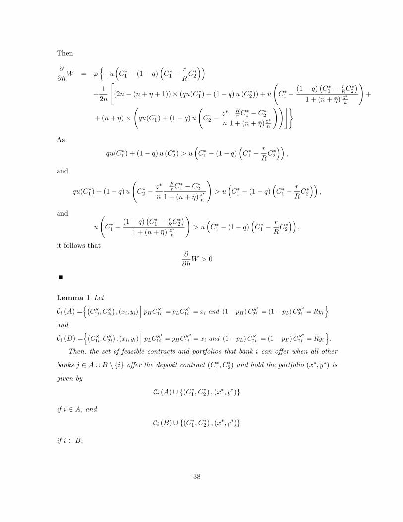
Then

∂

∂hW = ϕ

{−u(C∗1 − (1− q)

(C∗1 −

r

RC∗2

))+

1

2n

[(2n− (n+ η + 1))× (qu(C∗1 ) + (1− q)u (C∗2 )) + u

(C∗1 −

(1− q)(C∗1 − r

RC∗2

)1 + (n+ η) z

∗n

)+

+ (n+ η)×(qu(C∗1 ) + (1− q)u

(C∗2 −

z∗

n

Rr C∗1 − C∗2

1 + (n+ η) z∗n

))]}

As

qu(C∗1 ) + (1− q)u (C∗2 ) > u(C∗1 − (1− q)

(C∗1 −

r

RC∗2

)),

and

qu(C∗1 ) + (1− q)u(C∗2 −

z∗

n

Rr C∗1 − C∗2

1 + (n+ η) z∗n

)> u

(C∗1 − (1− q)

(C∗1 −

r

RC∗2

)),

and

u

(C∗1 −

(1− q)(C∗1 − r

RC∗2

)1 + (n+ η) z

∗n

)> u

(C∗1 − (1− q)

(C∗1 −

r

RC∗2

)),

it follows that∂

∂hW > 0

Lemma 1 Let

Ci (A) ={(CS1i, C

S2i

), (xi, yi)

∣∣∣ pHCS1

1i = pLCS2

1i = xi and (1− pH)CS1

2i = (1− pL)CS2

2i = Ryi

}and

Ci (B) ={(CS1i, C

S2i

), (xi, yi)

∣∣∣ pLCS1

1i = pHCS2

1i = xi and (1− pL)CS1

2i = (1− pH)CS2

2i = Ryi

}.

Then, the set of feasible contracts and portfolios that bank i can offer when all other

banks j ∈ A ∪B \ {i} offer the deposit contract (C∗1 , C∗2 ) and hold the portfolio (x∗, y∗) is

given by

Ci (A) ∪ {(C∗1 , C∗2 ) , (x∗, y∗)}

if i ∈ A, and

Ci (B) ∪ {(C∗1 , C∗2 ) , (x∗, y∗)}

if i ∈ B.

38

Proof. The derivations are provided for the case when i ∈ A. The case when i ∈ B

follows by symmetry and is omitted.

It is straightforward that the contract (C∗1 , C∗2 ) and the portfolio (x∗, y∗) are feasible.

Next I consider contracts(CS1i, C

S2i

)and portfolios (xi, yi) that are different then (C∗1 , C

∗2 )

and (x∗, y∗), and check which ones respect the feasibility constraints.

I first introduce some notation in order to express the feasibility constraints in matrix

form.

Let xA = (xi)i∈A, xB = (xi)i∈B, yA = (yi)i∈A and yB = (yi)i∈A be n × 1 column

vectors representing the liquid and illiquid asset holdings of banks in region A and B,

respectively.

Let ZA = (zij)i∈Aj∈A

be the n × n matrix of interbank deposits that banks in region A

hold at other banks in region A, with zij = 0 if i = j or if i and j do not have a link.

Similarly, I define ZB = (zij)i∈Bj∈B

be the n× n matrix of interbank deposits that banks in

region B hold at other banks in region B, with zij = 0 if i = j or if i and j do not have a

link. Let ZAB = (zij)i∈Aj∈B

be the n×n matrix of interbank deposits that banks in region A

hold at banks in region B, and ZBA = (zij)i∈Bj∈A

be the n× n matrix of interbank deposits

that banks in region B hold at banks in region A, with zij = 0 if i and j do not have a

link.

Let 1i be the n× 1 column vector that has all elements 0, except for the ith element

which is equal to 1. Let 1i×i be the n × n matrix with all elements 0, except for row i

which has all elements equal to 1. The identity matrix is denoted by I, while Ii represents

the identity matrix with all elements 0 on row i.

Then, when bank i offers a contract(CS1i, C

S2i

)and holds a portfolio (xi, yi) while all

other banks j ∈ A ∪ B \ {i} offer the deposit contract (C∗1 , C∗2 ) and hold the portfolio

(x∗, y∗), the feasibility constraints can be written for each date, state by state, as follows.

The date 0 feasibility constraint for banks in region A is

xA + yA + ZA · 1+ ZAB · 1 = 1+ ZTA · 1+ ZTBA · 1, (20)

while for banks in region B is

xB + yB + ZB · 1+ ZBA · 1 = 1+ ZTB · 1+ ZTAB · 1. (21)

39

The date 1 feasibility constraint for banks in region A is

xA + C∗1 · ZA · 1+C∗1 · ZAB · 1+(CS1

1i − C∗1

)· ZA · 1i = pHC

∗1 · 1+pH

(CS1

1i − C∗1

)· 1i + (22)

C∗1 · ZTA · 1+(CS1

1i − C∗1

)· 1i×i · ZA · 1i

in state S1, and

xA + C∗1 · ZA · 1+(CS2

1i − C∗1

)· ZA · 1i = pLC

∗1 · 1+pL

(CS2

1i − C∗1

)· 1i + (23)

C∗1 · ZTA · 1+ C∗1 · ZTBA · 1+(CS2

1i − C∗1

)· 1i×i · ZA · 1i +

(CS2

1i − C∗1

)· 1i×i · ZBA · 1i

in state S2.

The date 1 feasibility constraint for banks in region B is

xB + C∗1 · ZB · 1 = pLC∗1 · 1+ C∗1 · ZTB · 1+ C∗1 · ZTAB · 1 (24)

in state S1, and

xB + C∗1 · ZB · 1+C∗1 · ZBA · 1+(CS2

1i − C∗1

)· ZBA · 1i = pHC

∗1 · 1+ C∗1 · ZTB · 1 (25)

in state S2.

The date 2 feasibility constraint for banks in region A is

RyA = (1− pH)C∗2 ·1+ (1− pH)(CS1

2i − C∗2

)·1i+C∗2 ·ZTBA ·1+

(CS1

2i − C∗2

)·1i×i ·ZBA ·1i

(26)

in state S1, and

RyA + C∗2 · ZAB · 1 = (1− pL)C∗2 · 1+ (1− pL)(CS2

2i − C∗2

)· 1i (27)

in state S2.

The date 1 feasibility constraint for banks in region B is

RyB+C∗2 · ZBA · 1+(CS1

2i − C∗2

)· ZBA · 1i = (1− pL)C∗2 · 1 (28)

in state S1, and

RyB = (1− pH)C∗2 · 1+ C∗2 · ZTAB · 1 (29)

in state S2.

40

• Step 1: I first show that ZBA · 1i = 0.

Substracting (24) from (25), we obtain

ZBA · 1+ ZTAB · 1 = (pH − pL) · 1−

(CS2

1i − C∗1)

C∗1· ZBA · 1i

and, substracting (29) from (28), we obtain

ZBA · 1+ ZTAB · 1 = (pH − pL) · 1−

(CS1

2i − C∗2)

C∗2· ZBA · 1i

which implies that (CS1

2i − C∗2)

C∗2−

(CS2

1i − C∗1)

C∗1

· ZBA · 1i = 0 (30)

In addition, adding up (24) and (25), we obtain that

2xB+2C∗1 ·ZB·1+C∗1 ·ZBA·1+(CS2

1i − C∗1

)·ZBA·1i = (pH + pL)C∗1 ·1+2C∗1 ·ZTB ·1+C∗1 ·ZTAB·1.

Using that xB = qC∗1 · 1, and substituting q = pH+pL2 , we have

2 · ZB · 1+ZBA · 1+

(CS2

1i − C∗1)

C∗1· ZBA · 1i = 2 · ZTB · 1+ ZTAB · 1. (31)

Similarly, adding up (29) and (28), we obtain that

2RyB + C∗2 · ZBA · 1+(CS1

2i − C∗2

)· ZBA · 1i = (2− pL − pH)C∗2 · 1+ C∗2 · ZTAB · 1.

Using that yB =(1−q)C∗2

R · 1, and substituting q = pH+pL2 , we have

ZBA · 1+

(CS1

2i − C∗2)

C∗2· ZBA · 1i = ZTAB · 1 (32)

Adding up (31) and (32), we obtain that

2·ZB ·1+2·ZBA ·1+

(CS2

1i − C∗1)

C∗1·ZBA ·1i+

(CS1

2i − C∗2)

C∗2·ZBA ·1i = 2·ZTB ·1+2·ZTAB ·1

and since the date 0 feasibility constraint (21) implies that

ZB · 1+ ZBA · 1 =ZTB · 1+ ZTAB · 1

41

as xB + yB = 1, then we have that(CS1

2i − C∗2)

C∗2+

(CS2

1i − C∗1)

C∗1

· ZBA · 1i = 0 (33)

From (30) and (33), it follows that

ZBA · 1i = 0 (34)

• Step 2: I show that ZA · 1i = 0

Substracting (23) from (22) we obtain that

ZAB · 1+ ZTBA·1 = (pH − pL) · 1+

(pH

(CS1

1i − C∗1)− pL

(CS2

1i − C∗1))

C∗1· 1i +(

CS11i − C

S21i

)C∗1

· (1i×i − I) · ZA · 1i −

(CS2

1i − C∗1)

C∗1· 1i×i · ZBA · 1i,

and, substracting (27) from (26) we obtain that

ZAB · 1+ ZTBA · 1 = (pH − pL) · 1+

((1− pL)

(CS2

2i − C∗2)− (1− pH)

(CS1

2i − C∗2))

C∗2· 1i −(

CS12i − C∗2

)C∗2

· 1i×i · ZBA · 1i

Using (34), this implies that(pH

CS11i

C∗1− pL

CS21i

C∗1− (1− pL)

CS22i

C∗2+ (1− pH)

CS12i

C∗2

)·1i+

(CS1

1i − CS21i

)C∗1

·(1i×i − I)·ZA·1i = 0

which yields

ZA · 1i = 0 (35)

• Step 3: I show that 1T · ZTA · 1i = 0.

Using (34) and (35) in (22) and (23), respectively, and adding them up, we obtain

2xA + 2C∗1 · ZA · 1+C∗1 · ZAB · 1 = (pH + pL)C∗1 · 1+(pH

(CS1

1i − C∗1

)+ pL

(CS2

1i − C∗1

))· 1i +

2C∗1 · ZTA · 1+C∗1 · ZTBA · 1.

42

If we multiply this identity to the left both side with Ii, and make use that Ii ·xA =

qC∗1 · Ii · 1, we have that

2C∗1 · Ii · ZA · 1+C∗1 · Ii · ZAB · 1 = 2C∗1 · Ii · ZTA · 1+C∗1 · Ii · ZTBA · 1.

Further, multiplying to the left both side of (20) with Ii, and making use that

Ii · (xA + yA) = Ii · 1, we obtain that

Ii · ZA · 1+ Ii · ZAB · 1 =Ii · ZTA · 1+ Ii · ZTBA · 1, (36)

which implies, from the identity above, that

C∗1 · Ii · ZA · 1 = C∗1 · Ii · ZTA · 1.

We can simplify C∗1 and multiply on both side with 1T , and obtain

1T · Ii · ZA · 1 = 1T · Ii · ZTA · 1 (37)

or, since 1T · Ii = (1− 1i)T ,

(1− 1i)T · ZA · 1 = (1− 1i)T · ZTA · 1.

As 1T · ZA · 1 = 1T · ZTA · 1, it must be that

1Ti · ZA · 1 = 1Ti · ZTA · 1,

which, from (35), implies that

(1Ti · ZA · 1

)T= 0 (38)

• Step 4: I show that 1T · ZTAB · 1i = 0

Using (34) in (32), we obtain that

ZBA · 1 = ZTAB · 1.

The equations (36) and (37) imply that

Ii · ZAB · 1 =Ii · ZTBA · 1.

43

Adding-up these two identities, and multiplying to the left with 1T , we obtain

1T · ZBA · 1+ 1T · Ii · ZAB · 1 = 1T · ZTAB · 1+ 1T · Ii · ZTBA · 1

or, since 1T · Ii = 1T − 1Ti ,

1T · (ZBA + ZAB) · 1− 1Ti · ZAB · 1 = 1T ·(ZTBA + ZTAB

)· 1− 1Ti · ZTBA · 1.

As 1T · (ZBA + ZAB) · 1 = 1T ·(ZTBA + ZTAB

)· 1, then it follows that

1Ti · ZAB · 1 = 1Ti · ZTBA · 1,

which, from (34), implies that

(1Ti · ZAB · 1

)T= 0. (39)

The equations (34), (35), (38) and (39) imply that when bank i offers a contract(CS1i, C

S2i

)and holds a portfolio (xi, yi) while all other banks j ∈ A ∪ B \ {i} offer the

deposit contract (C∗1 , C∗2 ) and hold the portfolio (x∗, y∗), then bank i cannot hold any

interbank deposits at other banks, and other banks do not cannot hold interbank deposits

at bank i

zij = 0 and zji = 0, ∀j ∈ A ∪B.

The feasibility constraints for bank i become

xi + yi = 1

xi = pHCS1

1i = pLCS2

1i

Ryi = (1− pH)CS1

2i = (1− pL)CS2

2i .

Proof of Proposition 5.

To prove the result I show that there exists ϕ ∈ (0, 1) such that bank i’s best response

is to offer the deposit contract (1) and the portfolio (2) if all the other banks j 6= i offer

the deposit contract (1) and the portfolio (2), for any ϕ ≤ ϕ and for any i ∈ A ∪B.

The proof follows a similar argument as in the proof of Proposition 1 in Mailath,

Postlewaite and Samuelson (2005). The derivations are provided for the case when i ∈ A.

The case when i ∈ B follows by symmetry and is omitted.

44

From Lemma 1 above, we know that the set of feasible contracts and portfolios that

bank i can offer when all other banks j ∈ A ∪ B \ {i} offer the deposit contract (C∗1 , C∗2 )

and hold the portfolio (x∗, y∗) is given by

Ci (A) ∪ {(C∗1 , C∗2 ) , (x∗, y∗)} .

Note that the result in Lemma 1 does not rely on any assumption about the pattern of

interbank deposits between banks.

Then, I need to show that there exists ϕ ∈ (0, 1) such that

πi (g; (C∗1 , C∗2 ) , (x∗, y∗)) > πi

(g;(CS1i, C

S2i

), (xi, yi)

)for any ϕ ≤ ϕ, for any

(CS1i, C

S2i

), (xi, yi) ∈ CA, and for any g and g. Here I allow for the

possibility that a network g 6= g arises on the continuation path induced by the contract(CS1i, C

S2i

)and portfolio (xi, yi). The payoffs are given by

πi (g; (C∗1 , C∗2 ) , (x∗, y∗)) = (1− ϕ) [qu(C∗1 ) + (1− q)u(C∗2 )] + ϕugi ,

where ugi is the utility bank i obtains in the network g in state S, and

πi

(g;(CS1i, C

S2i

), (xi, yi)

)= (1− ϕ)

[1

2

(pHu(CS

1

1i ) + (1− pH)u(CS1

2i ))

+1

2

(pLu(CS

2

1i ) + (1− pL)u(CS2

2i ))]

+ϕugi ,

where ugi is the utility bank i obtains in the network g in state S,

Consider the function

f(t) =1

2

(pH ln t+ (1− pH) ln

(R (1− pHt)

(1− pH)

))+

1

2

(pL ln

(pHpLt

)+ (1− pL) ln

(R (1− pHt)

(1− pL)

)).

The function f is constructed such that

f(CS

1

1i

)=

1

2

(pHu(CS

1

1i ) + (1− pH)u(CS1

2i ))

+1

2

(pLu(CS

2

1i ) + (1− pL)u(CS2

2i )),

for any(CS1i, C

S2i

), (xi, yi) ∈ Ci (A). It is straightforward to show that10

maxtf (t) = f

(pH + pL

2pH

)= f

(q

pH

)10This follows from setting ∂f

∂t= 0. Note that t = pH+pL

2pHis indeed a maximum as ∂2f

∂t2

∣∣∣t=

pH+pL2pH

=

−4p2H

(2−pH−pL)(pH+pL)< 0.

45

where

f

(q

pH

)=

1

2

((1− pH) lnR

(1− q)1− pH

+ pH lnq

pH

)+

1

2

((1− pL) lnR

(1− q)1− pL

+ pL lnq

pL

)It follows that

f

(q

pH

)≥ 1

2

(pHu(CS

1

1i ) + (1− pH)u(CS1

2i ))

+1

2

(pLu(CS

2

1i ) + (1− pL)u(CS2

2i )),

for any(CS1i, C

S2i

), (xi, yi) ∈ Ci (A).

From Jensen’s inequality we obtain that

[(1− q) lnR]−[

1

2

((1− pH) lnR

(1− q)1− pH

+ pH lnq

pH

)+

1

2

((1− pL) lnR

(1− q)1− pL

+ pL lnq

pL

)]> 0

which implies, by the completeness of real numbers, that there exists a small number

ϕ′ > 0

[q ln 1 + (1− q) lnR]−[

1

2

((1− pH) lnR

(1− q)1− pH

+ pH lnq

pH

)+

1

2

((1− pL) lnR

(1− q)1− pL

+ pL lnq

pL

)]≥ ϕ′.

In other words, there exists a small (but independent of(CS1i, C

S2i

)) number ϕ′ > 0 such

that

[qu(C∗1 ) + (1− q)u(C∗2 )]−[

1

2

(pHu(CS

1

1i ) + (1− pH)u(CS1

2i ))

+1

2

(pLu(CS

2

1i ) + (1− pL)u(CS2

2i ))]≥ ϕ′,

(40)

for any(CS1i, C

S2i

), (xi, yi) ∈ CA, where I used that C∗1 = 1 and C∗2 = R.

Case 1: If ugi ≥ ugi it follows immediately that

πi (g; (C∗1 , C∗2 ) , (x∗, y∗)) > πi

(g;(CS1i, C

S2i

), (xi, yi)

)for any ϕ ∈ (0, 1).

Case 2: Suppose that ugi < ugi . Let

E ={

∆ > 0|∆ = ugi − ugi

}.

As consumption is finite, there exists

e ≡ sup(E) ∈ (0,∞).

Let

ϕ =ϕ′

ϕ′ + e

46

As ϕ′ > 0 and e <∞, then ϕ > 0. Then, for any ϕ ≤ ϕ

ϕ

1− ϕe ≤ϕ

1− ϕe

orϕ

1− ϕ

(ugi − u

gi

)≤ ϕ′.

From (40), we obtain that

[qu(C∗1 ) + (1− q)u(C∗2 )]−[

1

2

(pHu(CS

1

1i ) + (1− pH)u(CS1

2i ))

+1

2

(pLu(CS

2

1i ) + (1− pL)u(CS2

2i ))]≥ ϕ

1− ϕ

(ugi − u

gi

)or

πi (g; (C∗1 , C∗2 ) , (x∗, y∗)) > πi

(g;(CS1i, C

S2i

), (xi, yi)

)for any ϕ ≤ ϕ. Q.E.D.

Proof of Proposition 6.

Suppose that r < z∗(n+η)n((2z+1)(n+η)−1) . In the model with linking costs, each bank needs

to pay cost ε for each link. Thus, the total cost in a network gn,ηi , where each bank has ηi

links with banks in the same region, is∑2n

i=1 (ηi + n)× ε. Then, based on the derivations

of Proposition 4, the expected welfare in a network gn,ηi in which there are h banks that

have η links and (2n− h) banks that have less then η links is given by

W (gn,ηi ) = (1− ϕ) {2n× [qu (C∗1 ) + (1− q)u (C∗2 )]}

+ϕ

{2n− h

2n

[2n× u

(C∗1 − (1− q)

(C∗1 −

r

RC∗2

))]+h

2n

[(2n− (n+ η + 1))× (qu(C∗1 ) + (1− q)u (C∗2 )) + u

(C∗1 −

(1− q)(C∗1 − r

RC∗2

)1 + (n+ η) z

∗n

)

+ (n+ η)×(qu(C∗1 ) + (1− q)u

(C∗2 −

z∗

n

Rr C∗1 − C∗2

1 + (n+ η) z∗n

))]}

−2n∑i=1

(ηi + n)× ε.

As shown in the proof of Proposition 4, when the number of banks that have η links

increases from h to (h+ 1), there is an increases in the aggregate expected utility of

47

consumers of

ϕ{−u(C∗1 − (1− q)

(C∗1 −

r

RC∗2

))+

1

2n

[(2n− (n+ η + 1))× (qu(C∗1 ) + (1− q)u (C∗2 )) + u

(C∗1 −

(1− q)(C∗1 − r

RC∗2

)1 + (n+ η) z

∗n

)+

+ (n+ η)×(qu(C∗1 ) + (1− q)u

(C∗2 −

z∗

n

Rr C∗1 − C∗2

1 + (n+ η) z∗n

))]}.

At the same time, in the model with linking costs, the aggregate linking cost increases

as well. In particular, the maximum cost that can be associated with an equilibrium

interbank network in which there are (h+ 1) banks with η links is

(h+ 1)× η × 2ε+n× n

2× 2ε.

This is because in such an interbank network the number of links is maximized when

each bank in H(gn,ηi ) has links only with banks in {A ∪B} rH(gn,ηi ). Moreover, in an

equilibrium interbank network, banks that have less than η links have no links among

themselves (banks in {A ∪B} r H(gn,ηi ) have no links with other banks in {A ∪B} r

H(gn,ηi )).

In addition the minimum cost that can be associated with an equilibrium interbank

network in which there are h banks with η links is

h× η2× 2ε+

n× n2× 2ε.

This is because in such an interbank network the number of links is minimized when

each bank in H(gn,ηi ) has links only with banks in H(gn,ηi ). Moreover, in an equilibrium

interbank network, banks that have less than η links have no links among themselves.

This implies that as the number of banks that have η links increases from h to (h+ 1),

the aggregate linking cost can increase by at most

(h+ 2)× η × ε ≤ (2n+ 2)× η × ε.

It follows that the expected welfare in an equilibrium interbank network is increasing

48

in h when

ϕ{−u(C∗1 − (1− q)

(C∗1 −

r

RC∗2

))(41)

+1

2n

[(2n− (n+ η + 1))× (qu(C∗1 ) + (1− q)u (C∗2 )) + u

(C∗1 −

(1− q)(C∗1 − r

RC∗2

)1 + (n+ η) z

∗n

)+

+ (n+ η)×(qu(C∗1 ) + (1− q)u

(C∗2 −

z∗

n

Rr C∗1 − C∗2

1 + (n+ η) z∗n

))]}≥ (2n+ 2)× η × ε.

A suffi cient condition that insures that the welfare is increasing is given by

ϕ

{u

(C∗1 −

(1− q)(C∗1 − r

RC∗2

)1 + (n+ η) z

∗n

)− u

(C∗1 − (1− q)

(C∗1 −

r

RC∗2

))}> 3ε,

or

ϕ (1− q) ln

(R− z∗

n

Rr−R

1+(n+η) z∗n

)(1− (1− q) (1− r)) > 3ε, (42)

if investors have log preferences. If inequality (42) holds, then

ϕ× (2n− (n+ η + 1))× ((1− q) lnR− ln (1− (1− q) (1− r))) ≥ (2n− (n+ η + 1))× ε,

and

ϕ×(n+ η)×(

(1− q) ln

(R− z∗

n

Rr −R

1 + (n+ η) z∗n

)− ln (1− (1− q) (1− r))

)≥ (n+ η)×ε,

which insures that inequality (41) holds. By defining

ε ≡ 1

3ϕ (1− q) ln

(R− z∗

n

Rr−R

1+(n+η) z∗n

)(1− (1− q) (1− r)) ,

the proof is complete.

Appendix B: Proof of Proposition 2

A.1 Property 1.

Case 1: ηi ≥ η and ηj ≥ η

In this case, the marginal benefit that bank i receives from a link with bank j is given

by

πi(gn,ηi+ij)−πi(gn,ηi ) = (1− q)u(Cd2i(ηj + 1)

)+u(Cd1i(ηi + 1)

)−(1− q)u (C∗2 )−

(Cd1i(ηi)

).

49

Thus, Property 1 holds if

u

(C∗1 −

(1− q)(C∗1 − r

RC∗2

)1 + (n+ ηi + 1) z

∗n

)− u

(C∗1 −

(1− q)(C∗1 − r

RC∗2

)1 + (n+ ηi)

z∗n

)≤

(1− q)u (C∗2 )− (1− q)u(C∗2 −

z∗

n

Rr C∗1 − C∗2

1 + (n+ ηj + 1) z∗n

).

I establish this in three steps.

• Step 1: I show first that

u

(C∗1 −

(1− q)(C∗1 − r

RC∗2

)1 + (n+ ηi + 1) z

∗n

)− u

(C∗1 −

(1− q)(C∗1 − r

RC∗2

)1 + (n+ ηi)

z∗n

)≤

u

(C∗1 −

(1− q)(C∗1 − r

RC∗2

)1 + (n+ 1) z

∗n

)− u

(C∗1 −

(1− q)(C∗1 − r

RC∗2

)1 + n z

∗n

).

As

1

1 + (n+ ηi)z∗n

− 1

1 + (n+ ηi + 1) z∗n

≤

1

1 + (n+ ηi − 1) z∗n

− 1

1 + (n+ ηi)z∗n

.

then

1

2

(C∗1 −

(1− q)(C∗1 − r

RC∗2

)1 + (n+ ηi + 1) z

∗n

)+

1

2

(C∗1 −

(1− q)(C∗1 − r

RC∗2

)1 + (n+ ηi − 1) z

∗n

)≤

C∗1 −(1− q)

(C∗1 − r

RC∗2

)1 + (n+ ηi)

z∗n

.

and since u (·) is increasing, then

u

(1

2

(C∗1 −

(1− q)(C∗1 − r

RC∗2

)1 + (n+ ηi + 1) z

∗n

)+

1

2

(C∗1 −

(1− q)(C∗1 − r

RC∗2

)1 + (n+ ηi − 1) z

∗n

))≤

u

(C∗1 −

(1− q)(C∗1 − r

RC∗2

)1 + (n+ ηi)

z∗n

).

Using that u (·) is concave, and

1

2u

(C∗1 −

(1− q)(C∗1 − r

RC∗2

)1 + (n+ ηi + 1) z

∗n

)+

1

2u

(C∗1 −

(1− q)(C∗1 − r

RC∗2

)1 + (n+ ηi − 1) z

∗n

)≤

u

(1

2

(C∗1 −

(1− q)(C∗1 − r

RC∗2

)1 + (n+ ηi + 1) z

∗n

)+

1

2

(C∗1 −

(1− q)(C∗1 − r

RC∗2

)1 + (n+ ηi − 1) z

∗n

)).

50

we obtain that

u

(C∗1 −

(1− q)(C∗1 − r

RC∗2

)1 + (n+ ηi + 1) z

∗n

)− u

(C∗1 −

(1− q)(C∗1 − r

RC∗2

)1 + (n+ ηi)

z∗n

)≤

u

(C∗1 −

(1− q)(C∗1 − r

RC∗2

)1 + (n+ ηi)

z∗n

)− u

(C∗1 −

(1− q)(C∗1 − r

RC∗2

)1 + (n+ ηi − 1) z

∗n

),

for any ηi. This implies that

u

(C∗1 −

(1− q)(C∗1 − r

RC∗2

)1 + (n+ ηi + 1) z

∗n

)− u

(C∗1 −

(1− q)(C∗1 − r

RC∗2

)1 + (n+ ηi)

z∗n

)≤

u

(C∗1 −

(1− q)(C∗1 − r

RC∗2

)1 + (n+ 1) z

∗n

)− u

(C∗1 −

(1− q)(C∗1 − r

RC∗2

)1 + n z

∗n

).

• Step 2: As u (·) is increasing, it follows that

u (C∗2 )− u(C∗2 −

z∗

n

Rr C∗1 − C∗2

1 + (n+ ηj + 1) z∗n

)≥ u (C∗2 )− u

(C∗2 −

z∗

n

Rr C∗1 − C∗2

1 + (n+ n) z∗n

).

• Step 3: I show that in the case of log-utility function, the following inequality holds

u

(C∗1 −

(1− q)(C∗1 − r

RC∗2

)1 + (n+ 1) z

∗n

)− u

(C∗1 −

(1− q)(C∗1 − r

RC∗2

)1 + n z

∗n

)≤

(1− q)u (C∗2 )− (1− q)u(C∗2 −

z∗

n

Rr C∗1 − C∗2

1 + (n+ n) z∗n

).

In the case of a log-utility function, the optimal solution is given by

C∗1 = 1 and C∗2 = R

As

ln1− (1− r

RR)

1+(n+1) z∗n

1− (1− rRR)

1+n z∗n

≤ lnR

R− z∗n

Rr−R

1+(n+n) z∗n

and since

1

1− q ln1− (1−q)(1−r)

1+(n+1) z∗n

1− (1−q)(1−r)1+n z

∗n

51

is decreasing11 in q, then

1

1− q lnC∗1 −

(1−q)(C∗1−rRC∗2)

1+(n+1) z∗n

C∗1 −(1−q)(C∗1−

rRC∗2)

1+n z∗n

≤ lnC∗2

C∗2 − z∗n

RrC∗1−C∗2

1+(n+n) z∗n

.

Q.E.D.

Case 2: ηi ≤ η − 2 and ηj ≥ η

In this case, the marginal benefit that bank i receives from a link with bank j is given

by

πi(gn,ηi + ij)− πi(gn,ηi ) = (1− q)u(Cd2i(ηj + 1)

)+ u

(Cd1

)− (1− q)u (C∗2 )− u

(Cd1

).

Property 1 holds if

u (C∗2 ) > u

(C∗2 −

z∗

n

Rr C∗1 − C∗2

1 + (n+ ηj + 1) z∗n

)which is always true since u (·) is increasing.

Property 2.

Case 1: ηi ≥ η + 1 and ηj ≥ η + 1

In this case, the marginal benefit that bank i receives from severing a link with bank

j is given by

πi(gn,ηi−ij)−πi(gn,ηi ) = (1− q)u (C∗2 )+u(Cd1i(ηi − 1)

)−(1− q)u

(Cd2i(ηj)

)−(Cd1i(ηi)

).

Thus, Property 2 holds if

u

(C∗1 −

(1− q)(C∗1 − r

RC∗2

)1 + (n+ ηi)

z∗n

)− u

(C∗1 −

(1− q)(C∗1 − r

RC∗2

)1 + (n+ ηi − 1) z

∗n

)≤

(1− q)u (C∗2 )− (1− q)u(C∗2 −

z∗

n

Rr C∗1 − C∗2

1 + (n+ ηj)z∗n

).

The derivations are identical as for Property 1.

Case 2: ηi ≤ η − 1 and ηj ≥ η + 1

11The derivative with respect to q is

(q+z+(1−q)r)(z+nr+nz+nq(1−r)) ln

1− (1−q)(1−r)1+(n+1) z

n

1− (1−q)(1−r)1+n z

n

−z(1−r)(1−q)

(q−1)2(q+z+(1−q)r)(z+nr+nz+(1−r)nq) <

− nz(1−r)2(n+z+nz)(q+r+z−qr)(z+nq+nr+nz−nqr) , where I used that lnx < (x− 1) for any x > 0.

52

In this case, the marginal benefit that bank i receives from severing a link with bank

j is given by

πi(gn,ηi − ij)− πi(gn,ηi ) = (1− q)u (C∗2 ) + u(Cd1

)− (1− q)u

(Cd2i(ηj)

)− u

(Cd1

).

Property 2 holds if

u (C∗2 ) > u

(C∗2 −

z∗

n

Rr C∗1 − C∗2

1 + (n+ ηj)z∗n

)which is always true since u (·) is increasing.

Property 3.

Case 1: ηi ≥ η − 1 and ηj ≤ η − 1

When ηi = η− 1 and ηj = η− 1, the marginal benefit that bank i receives from a link

with bank j is given by

πi(gn,ηi + ij)− πi(gn,ηi ) = u(Cd1i(ηi + 1)

)+ u

(Cd2i(ηj + 1

))− u

(Cd1

)− u

(Cd1

).

When ηi = η− 1 and ηj ≤ η− 2, the marginal benefit that bank i receives from a link

with bank j is given by

πi(gn,ηi + ij)− πi(gn,ηi ) = u(Cd1i(ηi + 1)

)+ u

(Cd1

)− u

(Cd1

)− u

(Cd1

).

When ηi ≥ η and ηj = η − 1, the marginal benefit that bank i receives from a link

with bank j is given by

πi(gn,ηi + ij)− πi(gn,ηi ) = u(Cd1i(ηi + 1)

)+ u

(Cd2i(ηj + 1

))− u

(Cd1i (ηi)

)− u

(Cd1

).

When ηi ≥ η and ηj ≤ η − 2, the marginal benefit that bank i receives from a link

with bank j is given by

πi(gn,ηi + ij)− πi(gn,ηi ) = u(Cd1i(ηi + 1)

)+ u

(Cd1

)− u

(Cd1i (ηi)

)− u

(Cd1

).

Property 3 holds, as it follows from (12), (11), and (14) that

Cd2i(ηj + 1

)≥ C∗1 ≥ Cd1i(ηi + 1) ≥ Cd1i(ηi) ≥ Cd1 .

Case 2: ηi ≤ n− 1 and ηj = η − 1

53

When ηi ≥ η, the marginal benefit that bank i receives from a link with bank j is

given by

πi(gn,ηi + ij)− πi(gn,ηi ) = u(Cd1i(ηi + 1)

)+ u

(Cd2i(ηj + 1

))− u

(Cd1i(ηi)

)− u

(Cd1

).

When ηi = η − 1, the marginal benefit that bank i receives from a link with bank j is

given by

πi(gn,ηi + ij)− πi(gn,ηi ) = u(Cd1i(ηi + 1)

)+ u

(Cd2i(ηj + 1

))− u

(Cd1

)− u

(Cd1

).

When ηi ≤ η − 2, the marginal benefit that bank i receives from a link with bank j is

given by

πi(gn,ηi + ij)− πi(gn,ηi ) = u(Cd1

)+ u

(Cd2i(ηj + 1

))− u

(Cd1

)− u

(Cd1

).

Property 3 holds, as it follows from (12), (11), and (14) that

Cd2i(ηj + 1

)≥ C∗1 ≥ Cd1i(ηi + 1) ≥ Cd1i(ηi) ≥ Cd1 .

Property 4.

Case 1: ηi ≥ η and ηj ≤ η

When ηi = η and ηj = η, the marginal benefit that bank i receives from severing a

link with bank j is given by

πi(gn,ηi − ij)− πi(gn,ηi ) = u(Cd1

)+ u

(Cd1

)− u

(Cd1i(ηi)

)− u

(Cd2i(ηj)).

When ηi = η and ηj ≤ η − 1, the marginal benefit that bank i receives from severing

a link with bank j is given by

πi(gn,ηi − ij)− πi(gn,ηi ) = u(Cd1

)+ u

(Cd1

)− u

(Cd1i(ηi)

)− u

(Cd1

).

When ηi ≥ η + 1 and ηj = η, the marginal benefit that bank i receives from severing

a link with bank j is given by

πi(gn,ηi − ij)− πi(gn,ηi ) = u(Cd1i (ηi − 1)

)+ u

(Cd1

)− u

(Cd1i(ηi)

)− u

(Cd2i(ηj)).

54

When ηi ≥ η+1 and ηj ≤ η−1, the marginal benefit that bank i receives from severing

a link with bank j is given by

πi(gn,ηi − ij)− πi(gn,ηi ) = u(Cd1i(ηi − 1)

)+ u

(Cd1

)− u

(Cd1i (ηi)

)− u

(Cd1

).

Property 4 holds, as it follows from (12), (11), and (14) that

Cd2i(ηj + 1

)≥ C∗1 ≥ Cd1i(ηi + 1) ≥ Cd1i(ηi) ≥ Cd1 .

Case 2: ηi ≤ n− 1 and ηj = η

When ηi ≥ η + 1, the marginal benefit that bank i receives from severing a link with

bank j is given by

πi(gn,ηi − ij)− πi(gn,ηi ) = u(Cd1i(ηi − 1)

)+ u

(Cd1

)− u

(Cd1i(ηi)

)− u

(Cd2i(ηj)).

When ηi = η, the marginal benefit that bank i receives from severing a link with bank

j is given by

πi(gn,ηi − ij)− πi(gn,ηi ) = u(Cd1

)+ u

(Cd1

)− u

(Cd1i(ηi)

)− u

(Cd2i(ηj)).

When ηi ≤ η − 1, the marginal benefit that bank i receives from severing a link with

bank j is given by

πi(gn,ηi − ij)− πi(gn,ηi ) = u(Cd1

)+ u

(Cd1

)− u

(Cd1

)− u

(Cd2i(ηj)).

Property 4 holds, as it follows from (12), (11), and (14) that

Cd2i(ηj + 1

)≥ C∗1 ≥ Cd1i(ηi + 1) ≥ Cd1i(ηi) ≥ Cd1 .

Property 5.

ηi = η − 1 and ηj ≥ η if r <z∗(n+η)

n((2z+1)(n+η)−1) .

In this case, the marginal benefit that bank i receives from a link with bank j is given

by

πi(gn,ηi+ij)−πi(gn,ηi ) = (1− q)u(Cd2i(ηj + 1)

)+u(Cd1i(ηi + 1)

)−(1− q)u (C∗2 )−u

(Cd1

).

55

Property 5 holds if

u

(C∗1 −

(1− q)(C∗1 − r

RC∗2

)1 + (n+ ηi + 1) z

∗n

)− u

(C∗1 − (1− q)

(C∗1 −

r

RC∗2

))≤

(1− q)u (C∗2 )− (1− q)u(C∗2 −

z∗

n

Rr C∗1 − C∗2

1 + (n+ ηj + 1) z∗n

)I establish this in three steps.

• Step 1: As u (·) is increasing, it follows that

u (C∗2 )− u(C∗2 −

z∗

n

Rr C∗1 − C∗2

1 + (n+ ηj + 1) z∗n

)>

u (C∗2 )− u(C∗2 −

z∗

n

Rr C∗1 − C∗2

1 + 2z

)• Step 2: Next I show that

(1− q)u (C∗2 )− (1− q)u(C∗2 −

z∗

n

Rr C∗1 − C∗2

1 + 2z

)>

u

(C∗1 −

(1− q)(C∗1 − r

RC∗2

)1 + (n+ η) z

∗n

)− u

(C∗1 − (1− q)

(C∗1 −

r

RC∗2

))In the case of a log-utility function, the optimal solution is given by

C∗1 = 1 and C∗2 = R

As, by assumption,

r <z∗ (n+ η)

n ((2z + 1) (n+ η)− 1),

then

R

R− z∗n

Rr−R

1+2z

≥1− (1−r)

1+(n+η) z∗n

(1− (1− r)) .

Moreover, since

1

1− q ln1− (1−q)(1−r)

1+(n+η) z∗n

(1− (1− q) (1− r))is decreasing12 in q, then

lnC∗2

C∗2 − z∗n

RrC∗1−C∗21+2z

>1

1− q lnC∗1 −

(1−q)(C∗1−rRC∗2)

1+(n+η) z∗n(

C∗1 − (1− q)(C∗1 − r

RC∗2

)) .12The derivative with respect to q is

(q+(1−q)r)(z(η+n)+nq+(1−q)nr) ln

1− (1−q)(1−r)1+(n+η) z

n(1−(1−q)(1−r))−z(1−r)(1−q)(n+η)

(1−q)2(q+(1−q)r)(z(η+n)+nq+(1−q)nr) <

− nz(n+η)(1−r)2(n+z(η+n))(q+(1−q)r)(z(η+n)+nq+(1−q)nr) , where I used that lnx < (x− 1) for any x > 0.

56

Q.E.D.

There is still an issue of the existence of the parameter space. Note that, for a positive

η ≤ n− 1 to exist, inequality (13) implies that

Rz

z∗ + n (2z + 1) (R− 1)≤ r ≤ Rz

(R− 1)n (1 + z∗) +Rz.

As η is the smallest integer that satisfies (13), it follows that if

r −z∗(

(1−r)R−1

Rr −

nz∗ − n+ 1 + n

)n(

(2z + 1)(n+ (1−r)

R−1Rr −

nz∗ − n+ 1

)− 1) < 0, (43)

then

r <z∗ (η + n)

n ((2z + 1) (n+ η)− 1).

The inequality (43) holds for any r such that

f(r) =(−n2 (2z + 1) (R− 1)−Rnz − 2nz2

)r2+

(z∗2 − nz + 2Rnz2 + 2Rnz

)r−Rz2 < 0.

The f(r) is quadratic and concave in r, and it reaches a maximum for

rmax =z∗2 − nz + 2Rnz2 + 2Rnz

n2 (2z + 1) (R− 1) +Rnz + 2nz2.

It is then suffi cient if

f

(Rz

z∗ + n (2z + 1) (R− 1)

)< 0,

or, equivalently, if

R− 2n+ 2z − 4nz > 0,

to show that there exist r > Rzz∗+n(2z+1)(R−1) , such that f(r) < 0.

Property 6.

ηi = η and ηj ≥ η + 1 if r < z∗(n+η)n((2z+1)(n+η)−1) .

In this case, the marginal benefit that bank i receives from severing a link with bank

j is given by

πi(gn,ηi − ij)− πi(gn,ηi ) = (1− q)u (C∗2 ) + u(Cd1

)− (1− q)u

(Cd2i(ηj)

)− u

(Cd1i(ηi)

).

57

Property 6 holds if

u

(C∗1 −

(1− q)(C∗1 − r

RC∗2

)1 + (n+ ηi)

z∗n

)− u

(C∗1 − (1− q)

(C∗1 −

r

RC∗2

))≤

(1− q)u (C∗2 )− (1− q)u(C∗2 −

z∗

n

Rr C∗1 − C∗2

1 + (n+ ηj)z∗n

)

The derivations are identical as for Property 5.

Property 7.

ηi ≤ η − 2 and ηj ≤ η − 2

In this case, the marginal benefit that bank i receives from severing a link with bank

j is given by

πi(gn,ηi + ij)− πi(gn,ηi ) = u(Cd1

)+ u

(Cd1

)− u

(Cd1

)− u

(Cd1

),

or

πi(gn,ηi + ij) = πi(gn,ηi )

Property 8.

ηi ≤ η − 1 and ηj ≤ η − 1

In this case, the marginal benefit that bank i receives from severing a link with bank

j is given by

πi(gn,ηi − ij)− πi(gn,ηi ) = u(Cd1

)+ u

(Cd1

)− u

(Cd1

)− u

(Cd1

),

or

πi(gn,ηi − ij) = πi(gn,ηi )

58