Embed Size (px)
Citation preview

The Role and Nature of High Impact Events (Black
Swans): Technical Commentary and Empirical Data
N N Taleb
This is an appendix to the Edge piece. It is striking how some simple, simple tests (of stability of the 4th moment and failures of stress testing) can invalidate tens of
thousand of research papers on prediction using "least squares", and those based on "standard deviation", "variance", "correlation", "GARCH", "VAR", etc. Indeed one or
two tests can transform anything quantitative/statistical in social science (outside psychology) into facade of knowledge.
Introduction:
Data: Note that the analysis here is exhaustive: it is done systematically on almost ALL transacted macro data representing
>98% of worldwide volume. I used interest rates, commodities (oil, agricultural), all available equity indices (US, UK,
Continental Europe, Russia, Indonesia, Brazil), main traded currencies. I selected tradability because of its "cleanliness"
compared to merely computed data. I also added some micro data: although indices encompass single equities, I processed >18
million pieces of single stock daily data, and select industry datasuch as drug sales, movie returns, etc. (what "clean" data I
could find). While we have a plethora of data with business variables, we don't have enough in epidemics, terrorism, wars,
etc.
Logical and Mathematical Commentary
1) Telescope problem, insufficiency of data in the tails; consequence on left-skewed and right-skewed distributions;
2) Preasymptotics of probability distributions, classification of convergence, or why the central limit theorem is too Platonic;
What empirical data shows:
1) The severity of the fatness of the tails --and our inability to say "how" fat (my central problem). Not only kurtosis is> 3
everywhere;but it is unstable. One single observation in 10,000 represents 80% of the total fourth moment. Aside from the
unpredictability,this means that notions in Norm- (like variance,standard deviation,correlation) are meaningless as an
expression of any of the attributes of the probability distributions.
2) The "atypicality" of moves discussed in the article or why "stress testing" is dangerous--and why the data cannot be
captured by conventional "stress" tests or a Poisson except after the fact). Also while we are certain of power laws, we just can't
see the tails very clearly.
3) Past deviations (expressed in shortfalls) do not predict future deviations--at any lag you use collectively.There was no
need to do it but I tried anyway out of curiosity
Acknowledgments:These went into three pieces of formal technical work:a paper in the journal Complexity ( about the problem
of separation of fratal power laws into two basins and the effect of the preasymptotics of fat-tailed processes), another in the
International Journal of Forecasting ( about the role of measurement error with fat tails& what to do about it ), another under
review (about the problems of model selection when we only observe the data,not the process). The arguments were presented
at a special panel at the American Statistical Association Joint Statistical Meeting on August 6, 2008, in Denver.I thank Peter
Westfall,Aaron Brown,Stan Young, Donald Rubin,Robert Lund, for helpful discussions. I also thank Benoit Mandelbrot,David
Freedman,and Philip Stark for comments,and my long time colleague Pallop Angsupun for help with data.I thank David
Shaywitz for help with payoffs from innovation in drugs. I also thank Scott Patterson for alerting me to the "great moderation"
theories.
Mathematical Discussion
Definition of payoffs: Where probability is p(X), D the domain of the event, f(x) is the function of the payoff.
Using continuous distributions to simplify.
f(X) p(X) dX
Simple payoff f(x) =1 (a bet)
Complex payoff, expectation: f(x)=x
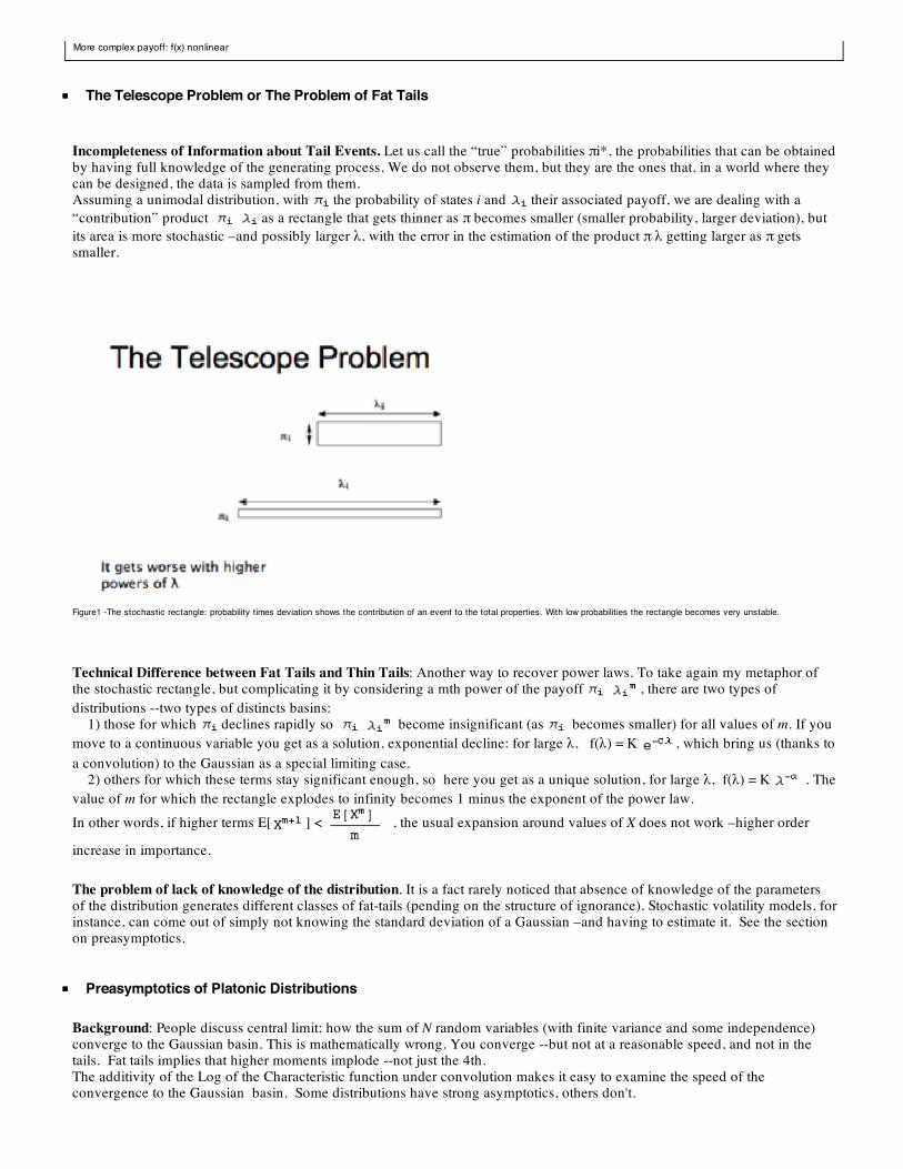
More complex payoff: f(x) nonlinear
The Telescope Problem or The Problem of Fat Tails
Incompleteness of Information about Tail Events. Let us call the “true” probabilities !i*, the probabilities that can be obtained
by having full knowledge of the generating process. We do not observe them, but they are the ones that, in a world where they
can be designed, the data is sampled from them.
Assuming a unimodal distribution, with the probability of states i and their associated payoff, we are dealing with a
“contribution” product as a rectangle that gets thinner as ! becomes smaller (smaller probability, larger deviation), but
its area is more stochastic –and possibly larger ", with the error in the estimation of the product ! " getting larger as ! gets
smaller.
Figure1 -The stochastic rectangle: probability times deviation shows the contribution of an event to the total properties. With low probabilities the rectangle becomes very unstable.
Technical Difference between Fat Tails and Thin Tails: Another way to recover power laws. To take again my metaphor of
the stochastic rectangle, but complicating it by considering a mth power of the payoff , there are two types of
distributions --two types of distincts basins:
1) those for which declines rapidly so become insignificant (as becomes smaller) for all values of m. If you
move to a continuous variable you get as a solution, exponential decline: for large ", f(") = K , which bring us (thanks to
a convolution) to the Gaussian as a special limiting case.
2) others for which these terms stay significant enough, so here you get as a unique solution, for large ", f(") = K . The
value of m for which the rectangle explodes to infinity becomes 1 minus the exponent of the power law.
In other words, if higher terms E[ ] < , the usual expansion around values of X does not work –higher order
increase in importance.
The problem of lack of knowledge of the distribution. It is a fact rarely noticed that absence of knowledge of the parameters
of the distribution generates different classes of fat-tails (pending on the structure of ignorance). Stochastic volatility models, for
instance, can come out of simply not knowing the standard deviation of a Gaussian –and having to estimate it. See the section
on preasymptotics.
Preasymptotics of Platonic Distributions
Background: People discuss central limit: how the sum of N random variables (with finite variance and some independence)
converge to the Gaussian basin. This is mathematically wrong. You converge --but not at a reasonable speed, and not in the
tails. Fat tails implies that higher moments implode --not just the 4th.
The additivity of the Log of the Characteristic function under convolution makes it easy to examine the speed of the
convergence to the Gaussian basin. Some distributions have strong asymptotics, others don't.
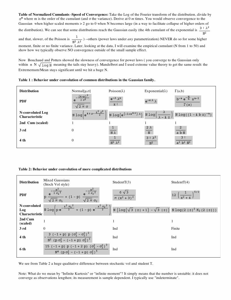
Table of Normalized Cumulants -Speed of Convergence: Take the Log of the Fourier transform of the distribution, divide by
where m is the order of the cumulant (and ! the variance). Derive at 0 m times. You would observe convergence to the
Gaussian when higher scaled moments > 2 go to 0 when N becomes large (in a way to facilitate collapse of higher orders of
the distribution). We can see that some distributions reach the Gaussian easily (the 4th cumulant of the exponential is
and that, slower, of the Poisson is ) --others (power laws under any parametrization) NEVER do so for some higher
moment, finite or no finite variance. Later, looking at the data, I will examine the empirical cumulant (N from 1 to 50) and
show how we typically observe NO convergence outside of the small sample effect.
Now Bouchaud and Potters showed the slowness of convergence for power laws ( you converge to the Gaussian only
within ± N meaning the tails stay heavy). Mandelbrot and I used extreme value theory to get the same result: the
Extrememum/Mean stays significant until we hit a huge N.
Table 1 : Behavior under convolution of common distributions in the Gaussian family.
Distribution Normal[",!] Poisson(#) Exponential(#) $(a,b)
N-convoluted Log
Characteristic
2nd Cum (scaled) 1 1 1 1
3 rd 0
4 th 0
Table 2: Behavior under convolution of more complicated distributions
DistributionMixed Gaussians
(Stoch Vol style)StudentT(3) StudentT(4)
N-convoluted
Log
Characteristic
2nd Cum
(scaled)1 1 1
3 rd 0 Ind Finite
4 th Ind Ind
6 th Ind Ind
We see from Table 2 a huge qualitative difference between stochastic vol and student T.
Note: What do we mean by "Infinite Kurtosis" or "infinite moment"? It simply means that the number is unstable; it does not
converge as observations lengthen; its measurement is sample dependent. I typically use "indeterminate".

Letting the Data Speak
Sampling Error of the Fourth Moment
Kurtosis in the normal framework implies "departure from Gaussian". So can you imagine that people talk about "kurtosis" --
and measure it -- when one single observation in 40 years (10,000 data points) can represent 90% of the properties!
The implication is that 1) most of the work about fat tails 2) any measure of "volatility" in L2 is just inoperative!
I take here the maximum variable to the fourth power to see its contribution to the kurtosis. For a Gaussian,with
N~ the number is expected to be ridiculously small, ~.008.
Implication: we don't know how "fat" the tails are --if we want to stay in the regular world of assuming that a distribution has
three attributes: centrality, dispersion, symmetry. But we need a fourth dimension: tail indicator, and power laws have it. So,
again, we need to escape the L2 norm.
This also tells us that GARCH should not work --indeed it DOES NOT work out of sample.

In the Gaussian World it has a small dispersion, around .008 for N=10,000 (see simulation of times the N, for a total of
). Even then one observation in 10,000 synthetic securities reoresented a max ~ .037.
Saying "Fat Tails" Implies Difficulties with the Distribution
The instability of The Fourth moment. We have KURT the "raw" Kurtosis for daily observations, KURT10 for biweekly ones,
and KURT66 for 3 month observations of Log changes in the macro variables. " Max Quartic" is the measure of the maximal
contribution to the fourth moment coming from one single observation
KURT KURT10 KURT66 Max Quartic
Australian Dollar 6.3 3.8 2.9 0.12 22.
Australia TB 10y 7.5 6.2 3.5 0.08 25.
Australia TB 3y 7.5 5.4 4.2 0.06 21.
BeanOil 5.5 7. 4.9 0.11 47.
Bonds 30Y 5.6 4.7 3.9 0.02 32.
Bovespa 24.9 5. 2.3 0.27 16.
British Pound 6.9 7.4 5.3 0.05 38.
CAC40 6.5 4.7 3.6 0.05 20.
Canadian Dollar 7.4 4.1 3.9 0.06 38.
Cocoa NY 4.9 4. 5.2 0.04 47.

Coffee NY 10.7 5.2 5.3 0.13 37.
Copper 6.4 5.5 4.5 0.05 48.
Corn 9.4 8. 5. 0.18 49.
CrudeOil 29. 4.7 5.1 0.79 26.
CT 7.8 4.8 3.7 0.25 48.
DAX 8. 6.5 3.7 0.2 18.
Euro Bund 4.9 3.2 3.3 0.06 18.
Euro Curr 5.5 3.8 2.8 0.06 38.
Eurodollar Depo 1M 41.5 28. 6. 0.31 19.
Eurodollar Depo 3M 21.1 8.1 7. 0.25 28.
FTSE 15.2 27.4 6.5 0.54 25.
Gold 11.9 14.5 16.6 0.04 35.
Heating Oil 20. 4.1 4.4 0.74 31.
Hogs 4.5 4.6 4.8 0.05 43.
Jakarta Stock Index 40.5 6.2 4.2 0.19 16.
JGB 17.2 16.9 4.3 0.48 24.
Live Cattle 4.2 4.9 5.6 0.04 44.
Nasdaq 11.4 9.3 5. 0.13 21.
NatGas 6. 3.9 3.8 0.06 19.
Nikkei 52.6 4. 2.9 0.72 23.
Notes 5Y 5.1 3.2 2.5 0.06 21.
Russia RTSI 13.3 6. 7.3 0.13 17.
Short Sterling 851.8 93. 3. 0.75 17.
Silver 160.3 22.6 10.2 0.94 46.
smallcap 6.1 5.7 6.8 0.06 17.
SoyBeans 7.1 8.8 6.7 0.17 47.
SoyMeal 8.9 9.8 8.5 0.09 48.
sp500 38.2 7.7 5.1 0.79 56.
Sugar #11 9.4 6.4 3.8 0.3 48.
SwissFranc 5.1 3.8 2.6 0.05 38.
TY10Y Notes 5.9 5.5 4.9 0.1 27.
Wheat 5.6 6. 6.9 0.02 49.
Yen 9.7 6.1 2.5 0.27 38.
Behavior of the Fourth Moment under temporal aggregation
The discussion of the preasymptotics table shows the theoretical effect of Central Limit if it worked. --Yet we see NONE
beyond the regular sampling error with "infinite" (i.e. non existing) moments.
With !t as the lag in days (here the lag is 1 through 45):
Slight technicity: I avoid the notion of ex post "mean" in the computation of Kurtosis. Most of the data is continuous futures
with 0 expected mean. The data I used is mostly "continuous future"


Note Some data is "controlled", making it less wild, owing to circuit breakers (markets shut down if they move more than, say 3
points), which causes an artificial thinning of the tails and lowers the Maximum Quartic contrbution. For instance Oct 20 1987,
the 30y bond moved 10 points in the real market, but only a move of 3 was registered as the circuit breakers were activated.
Longitudinal 4th moment: no sign of stability. Typical graph.
First Conclusion: Avoid the use of "variance" metrics. mean-variance is inadequate.
Evidence of Scalability - or Why Observed "Fat Tails" are not (Standard) Poisson and why there is no TYPICAL
deviation
Thanks to the need for the probabililities add up to 1 (something even economists seem to agree with), scalability in the tails is

the sole possible model for such data. We may not be able to write the model for the full distribution --but we know how it
looks like in the tails, where it matters.
The Behavior of Conditional Averages: With a scalable (or "scale-free") distribution, when K is "in the tails" (say you reach
the point when f[x,!]=C , where C is a constant and ! the power law exponent), the relative conditional expectation of X
(knowing that x>K) divided by K, that is, is a constant, and does not depend on K. More precisely, it is
.
This provides for a handy way to ascertain scalability by raising K and looking at the averages in the data.
Note further that, for a standard Poisson, (too obvious for a Gaussian): not only the conditional expectation depends on K, but it
"wanes", i.e.
Other Decompositions: The result of course would cancel the kind of representations such as the model called Duffie-Pan-
Singleton, which decomposes generating processes into a sum of jumps and some diffusion. Unless they have an infinity of
power-law sized jumps, the conditional average would lose its scalability beyond the worst jump.
Calibrating Tail Exponents. In addition, we can calibrate power laws. Using K as the cross-over point, we get the ! exponent
above it --the same as if we used the Hill estimator or ran a regression above some point.
Individual Stocks Data
Stocks are interesting because there are so many. This test using 12 million pieces of exhaustive single stock returns shows how
equity prices do not have a characteristic scale.No other possible method than a Paretan tail,albeit of unprecise calibration,can
charaterize them.
Data: Pallop Angsupun ran the following test: We collected the most recent 10 years of daily prices for stocks (no survivorship
bias effect as we included companies that have been delisted up to the last trading day), n= 11,674,825 , deviations expressed
in logarithmic returns.
We focused on negative deviations. For instance,in the Table x below,the average move below "10 standard deviations",-10,is -
15.6 standard deviations, that is a multiple of 1.56.We kept moving K up until to 100 "sigmas" equivalent (indeed) --and we
still had observations.
Note the tail estimator
Daily Returns (Stocks)
I normalized by STD (to communicate the result in the lingo) but we get the same results with MAD
Sigma n Implied !
-1. -1.74525 1.5242*10^^6 1.74525 2.34183
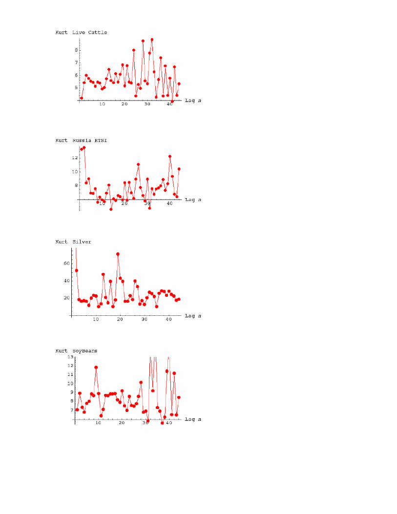
-2. -3.01389 343952. 1.50695 2.9726
-3. -4.58148 99404. 1.52716 2.89696
-10. -15.6078 3528. 1.56078 2.78324
-20. -30.4193 503. 1.52096 2.91952
-50. -113.324 20. 2.26649 1.78958
-75. -180.84 9. 2.4112 1.70861
-100. -251.691 5. 2.51691 1.65923
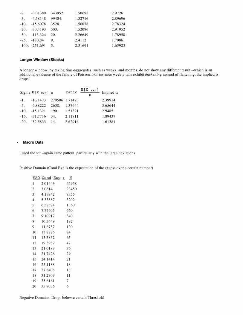
Longer Window (Stocks)
A longer window, by taking time-aggregates, such as weeks, and months, do not show any different result --which is an
additional evidence of the failure of Poisson. For instance weekly tails exhibit thickening instead of flattening: the implied !
drops!
Sigma n Implied !
-1. -1.71473 270506. 1.71473 2.39914
-5. -6.88222 2638. 1.37644 3.65644
-10. -15.1321 190. 1.51321 2.9485
-15. -31.7716 34. 2.11811 1.89437
-20. -52.5833 14. 2.62916 1.61381
Macro Data
I used the set --again same pattern, particularly with the large deviations.
Positive Domain (Cond Exp is the expectation of the excess over a certain number)
1 2.01443 65958
2 3.0814 23450
3 4.19842 8355
4 5.33587 3202
5 6.52524 1360
6 7.74405 660
7 9.10917 340
8 10.3649 192
9 11.6737 120
10 13.8726 84
11 15.3832 65
12 19.3987 47
13 21.0189 36
14 21.7426 29
15 24.1414 21
16 25.1188 18
17 27.8408 13
18 31.2309 11
19 35.6161 7
20 35.9036 6
Negative Domains: Drops below a certain Threshold
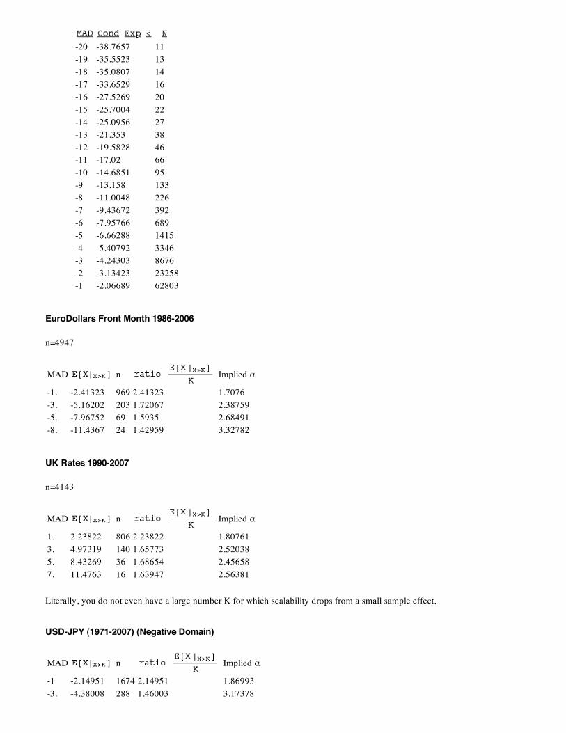
-20 -38.7657 11
-19 -35.5523 13
-18 -35.0807 14
-17 -33.6529 16
-16 -27.5269 20
-15 -25.7004 22
-14 -25.0956 27
-13 -21.353 38
-12 -19.5828 46
-11 -17.02 66
-10 -14.6851 95
-9 -13.158 133
-8 -11.0048 226
-7 -9.43672 392
-6 -7.95766 689
-5 -6.66288 1415
-4 -5.40792 3346
-3 -4.24303 8676
-2 -3.13423 23258
-1 -2.06689 62803
EuroDollars Front Month 1986-2006
n=4947
MAD n Implied !
-1. -2.41323 969 2.41323 1.7076
-3. -5.16202 203 1.72067 2.38759
-5. -7.96752 69 1.5935 2.68491
-8. -11.4367 24 1.42959 3.32782
UK Rates 1990-2007
n=4143
MAD n Implied !
1. 2.23822 806 2.23822 1.80761
3. 4.97319 140 1.65773 2.52038
5. 8.43269 36 1.68654 2.45658
7. 11.4763 16 1.63947 2.56381
Literally, you do not even have a large number K for which scalability drops from a small sample effect.
USD-JPY (1971-2007) (Negative Domain)
MAD n Implied !
-1 -2.14951 1674 2.14951 1.86993
-3. -4.38008 288 1.46003 3.17378

-5. -6.74883 66 1.34977 3.85906
-6. -7.92747 34 1.32125 4.11288
-8.75 -13.2717 6 1.51677 2.9351
We get scalability as far as meets the eye. Usually small sample effects cause us to not observe much of the tails, with the
consequence of "thinning" the upper bound. We do not even witness such effect.
Past ShortFall Does not Predict Future ShortFall -at all lags
The picture shows the predictability of a 7% shortfall, i.e. on , = if X <-.07. With discrete data, we
see if a given shortfall after a date t can be predicted from data before that date t. Here X= Log[ / ]. The result is
presented in Log space. Note that here !t = 1day and I lagged by 252 days. But the result does not change in a perceptible way
when I change the observation period or vary the lag (next Graph).
Lagging does not help. Except that one my datamining might be able to find some "rule" but these have failed out of sample.

However regular events tend to predict regular events
The graph shows the predictability of mean deviation between one period (252 days) and the next.
A Brief Discussion of Drug and Movie Successes
I look at drug sales for existing drugs. The problem is that when the Max is 167 STD away from the mean, you have a problem.
That number could double if I include some marginal drugs not in my sample as these would affect the mean. I coulf not get a
convincing tail exponent.
Max 1.34*10^^10
Total 4.93777*10^^11
Mean 3.98583*10^^6
Max/STD 167.633
MAD 7.19047*10^^6
STD 7.99363*10^^7
With movies it is even worse. We don't know the baseline.
n 7985.
Max 6.00788*10^^8
Total 1.16288*10^^11
Mean 1.45633*10^^7
Max/STD 17.598
MAD 1.90327*10^^7
STD 3.41395*10^^7
But I can derive conclusions: there is a " potential" in the tails that I could fill-in --which would raise the expected mean
considerably. But how much? I don't know and I don't want to play like academic charlatans.

Created by Mathematica (September 21, 2008)