The Frequency of Supernovae in the Early Universesu.diva-portal.org/smash/get/diva2:410152/FULLTEXT01.pdf · supernova candidates, making the observations even more time-consuming

The Frequency of Supernovae inthe Early Universe

Jens Melinder

Department of Astronomy

Stockholm University

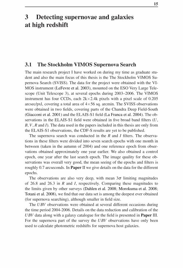
Cover image:The three images show a supernova discovered by the Stockholm VIMOSSupernova Survey. The upper left image and right images show athree-colour composite of the host galaxy region before and after thesupernova exploded, respectively. The lower image shows the differencebetween the two images.Image credit:The SVISS team, based on observations with the VLT/VIMOS instrument atParanal, Chile, operated by the European Southern Observatories.

Jens Melinder, Stockholm 2011ISBN 978-91-7447-274-5Printed in Sweden by Universitetsservice, US-AB, Stockholm 2011Distributor: Department of Astronomy, Stockholm University

Doctoral Dissertation 2011

Department of Astronomy

Stockholm University

SE-106 91 Stockholm

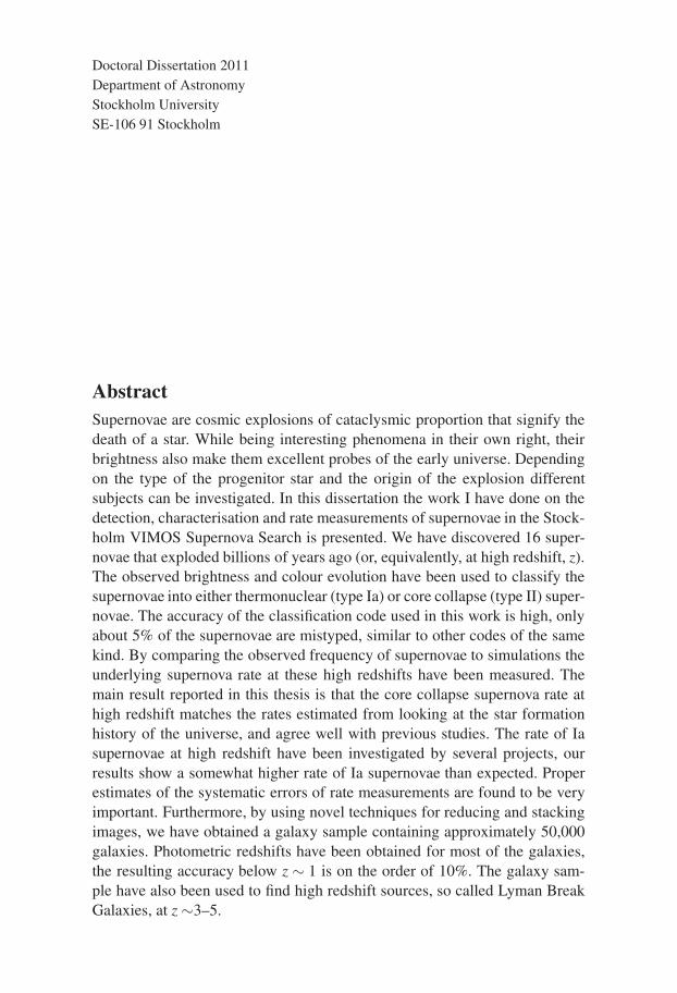
AbstractSupernovae are cosmic explosions of cataclysmic proportion that signify thedeath of a star. While being interesting phenomena in their own right, theirbrightness also make them excellent probes of the early universe. Dependingon the type of the progenitor star and the origin of the explosion differentsubjects can be investigated. In this dissertation the work I have done on thedetection, characterisation and rate measurements of supernovae in the Stock-holm VIMOS Supernova Search is presented. We have discovered 16 super-novae that exploded billions of years ago (or, equivalently, at high redshift, z).The observed brightness and colour evolution have been used to classify thesupernovae into either thermonuclear (type Ia) or core collapse (type II) super-novae. The accuracy of the classification code used in this work is high, onlyabout 5% of the supernovae are mistyped, similar to other codes of the samekind. By comparing the observed frequency of supernovae to simulations theunderlying supernova rate at these high redshifts have been measured. Themain result reported in this thesis is that the core collapse supernova rate athigh redshift matches the rates estimated from looking at the star formationhistory of the universe, and agree well with previous studies. The rate of Iasupernovae at high redshift have been investigated by several projects, ourresults show a somewhat higher rate of Ia supernovae than expected. Properestimates of the systematic errors of rate measurements are found to be veryimportant. Furthermore, by using novel techniques for reducing and stackingimages, we have obtained a galaxy sample containing approximately 50,000galaxies. Photometric redshifts have been obtained for most of the galaxies,the resulting accuracy below z ∼ 1 is on the order of 10%. The galaxy sam-ple have also been used to find high redshift sources, so called Lyman BreakGalaxies, at z ∼3–5.

Though my soul may set in darkness,

it will rise in perfect light.

I have loved the stars too fondly

to be fearful of the night.

”The Old Astronomer to his Pupil” by Sarah Williams.

To Moa

7

List of Papers

This thesis is based on the following papers, which are referred to in the textby their Roman numerals.

I Detection efficiency and photometry in supernova surveys –the Stockholm VIMOS Supernova Survey IMelinder J., Mattila S.,Östlin G., Mencía Trinchant L., FranssonC., 2008, A&A, 490, 419M

II The discovery and classification of 16 supernovae at high red-shifts in ELAIS-S1 – the Stockholm VIMOS Supernova Sur-vey IIMelinder J., Dahlen T., Mencía Trinchant L., Östlin G., MattilaS., Sollerman J., Fransson C., Hayes M., Nasoudi-Shoar S., 2011,submitted to A&A

III Deep UBVRI observations of a field within ELAIS-S1 – theStockholm VIMOS Supernova Survey IIIMencía-Trinchant L., Melinder J., Dahlen T., Östlin G., FranssonC., Nasoudi-Shoar S., Hayes M., Mattila S., 2011, A&A to besubmitted

IV The Rate of Supernovae at Redshift z ∼ 0.1 − 1.0 – theStockholm VIMOS Supernova Survey IVMelinder J., Dahlen T., Mencía Trinchant L., Östlin G., MattilaS., Sollerman J., Fransson C., Hayes M., Nasoudi-Shoar S.,2011, A&A to be submitted

Contents

1 Introduction 11.1 Observational astronomy, magnitudes and colours . . . . . . . . . 31.2 Cosmology – redshift, distance and look back Time . . . . . . . . 4

2 Supernova physics — a brief review 72.1 Core collapse supernovae . . . . . . . . . . . . . . . . . . . . . . . . . . . . 7

2.1.1 IIP and IIL supernovae . . . . . . . . . . . . . . . . . . . . . . . . 102.1.2 Ib and Ic supernovae . . . . . . . . . . . . . . . . . . . . . . . . . 112.1.3 IIn supernovae . . . . . . . . . . . . . . . . . . . . . . . . . . . . . . 11

2.2 Thermonuclear supernovae . . . . . . . . . . . . . . . . . . . . . . . . . . . 12

3 Detecting supernovae and galaxies at high redshift 153.1 The Stockholm VIMOS Supernova Search . . . . . . . . . . . . . . . 153.2 Observational astronomy at a glance — imaging surveys . . . . 16

3.2.1 Image data reduction . . . . . . . . . . . . . . . . . . . . . . . . . 173.2.2 Source detection and photometry . . . . . . . . . . . . . . . . 18

3.3 Studying galaxies with surveys . . . . . . . . . . . . . . . . . . . . . . . . 193.3.1 Number counts . . . . . . . . . . . . . . . . . . . . . . . . . . . . . 193.3.2 Photometric redshifts . . . . . . . . . . . . . . . . . . . . . . . . . 213.3.3 Lyman break galaxies . . . . . . . . . . . . . . . . . . . . . . . . 21

3.4 How to find supernovae . . . . . . . . . . . . . . . . . . . . . . . . . . . . . 233.4.1 Image subtraction . . . . . . . . . . . . . . . . . . . . . . . . . . . 233.4.2 Detection and photometry of supernovae . . . . . . . . . . 26

4 Photometric Classification of Supernovae 294.1 Examples of photometric supernova typing in the literature . . 294.2 Supernova light curve templates . . . . . . . . . . . . . . . . . . . . . . . 304.3 Bayesian typing of supernovae . . . . . . . . . . . . . . . . . . . . . . . . 31

5 Supernova Rates 375.1 Earlier work on supernova rates . . . . . . . . . . . . . . . . . . . . . . . 375.2 Methods of estimating rates . . . . . . . . . . . . . . . . . . . . . . . . . . 385.3 Comparing supernova rates to the star formation history . . . . . 395.4 Constraining the Ia delay time distribution . . . . . . . . . . . . . . . 415.5 Systematic errors for rate measurements . . . . . . . . . . . . . . . . . 42

10 CONTENTS

5.5.1 Contamination by AGN . . . . . . . . . . . . . . . . . . . . . . . 435.6 The effect of host galaxy extinction on the rates . . . . . . . . . . . 44

6 Summary of the papers 47

7 Svensk sammanfattning av avhandlingen 49

Publications not included in this thesis 51

Acknowledgements 53

Bibliography 55

1

1 Introduction

Supernova explosions are among the most energetic events known tomankind. During the explosion the supernova can reach luminosities that rivalthe brightness of the host galaxy. However, this extreme luminosity is onlyfleeting, as the explosion shock wave tears through the material surroundingthe core of the star, the supernova will become fainter and fainter until it isno longer detectable. Depending on the origin of the explosion, essentiallywhat kind of progenitor star that exploded, the length of time the supernovastays bright and what remains afterwards will be different. The two maintypes of supernovae are: core collapse supernovae (CC SNe), massive starsthat undergo gravitational collapse as they run out of fuel followed by anexplosion (e.g., Nomoto 1984); and thermonuclear supernovae (or Ia SNe),white dwarfs that collapse and explode when they accrete too much matter(e.g., Leibundgut 2000).

Supernovae, being very bright and relatively long-lived phenomena, havelikely been observed by humans for as long as we have looked at the sky. Forthe early astronomers the rare event of a supernova going off in the Milky way(and detectable to the naked eye from Earth) must have been awe-striking. Thevery first written reports on supernovae are from Chinese Imperial records,where the earliest probable supernova found is one that exploded in AD 185.There were a number of supernovae (5–10) reported by both Oriental and Eu-ropean astronomers up until the last one in AD 1604 (Stephenson & Green2005), since then none have been detected within our galaxy. However, in1987 a new bright variable object was found in the Large Magellanic Cloud.It turned out to be the most nearby supernova observed in modern times (seeArnett et al. 1989, for a review) and the importance of the discovery to super-nova astrophysics can hardly be understated.

The supernovae studied in my research are located in other galaxies at fargreater distances. The light from these explosions travel through the universeat the speed of light to reach our telescopes. When the light finally reachesus the travel time can have reached billions of years, the supernovae discov-ered in our search exploded approximately six billion years ago. We use thesupernovae as probes of the Universe at this earlier epoch in its history. Thefrequency of CC SNe, and Ia SNe to some extent, are coupled to the starformation in these faraway galaxies (see, e.g, Dahlen et al. 2004). By find-ing supernovae, that in some cases are easier to find and characterise than the

2 Introduction

galaxies themselves, we can put constraints on the formation of stars in theearly universe.

The frequency, or rate, of supernovae in a given cosmic volume can bemeasured by counting the number of SNe discovered within a specific regionon the sky and dividing by the time span over which the observations havebeen made. The very first measures of supernova rates were done by Zwicky(1938), who found that “the average frequency of occurrence of supernovaeis about one supernovae per extra-galactic nebula per six hundred years” forthe local volume of space. More recently, several measurements of the rate ofboth CC and Ia SNe in the local Universe (e.g., Li et al. 2011a) and in the earlyuniverse (e.g., Dahlen et al. 2004) have been published. The results publishedin the papers that are part of this thesis add to the measurements in the earlyuniverse.

In my research I have made use of the European Southern Observatories(ESO) telescope VLT (Very Large Telescope) in Chile and the instrument VI-MOS (VIsible MultiObject Spectrograph) mounted on one of the four 8.2-metre telescopes that make up the VLT. We have used this instrument inimaging mode to look at a patch in the sky in different colours. By regularmonitoring of the same field over a longer period of time it is possible to de-tect supernovae that explode in the otherwise perfectly unchanging galaxies.This method to discover supernovae is common practice, it’s main benefit isthat observations of the same patch in the sky over a controlled time span al-lows the observer to minimise possible bias effects. The main drawback is ofcourse that such a project is observationally expensive, requiring many hoursof valuable telescope time to complete. In many cases supernova imaging sur-veys are also complemented by follow-up spectroscopic observations of thesupernova candidates, making the observations even more time-consuming.In our survey we do not obtain spectra for the supernovae, instead relying onimaging data only to make our analysis.

This thesis is divided into five chapters, the first being the Introduction.The second chapter, Supernova physics — a brief review, contains somebasic theory on supernovae. In the third chapter, Detecting supernovae andgalaxies at high redshift, I go through how survey observations are used tofind supernovae and study galaxies. The fourth chapter, Photometric classifi-cation of supernovae, deals with methods for classifying discovered sourcesinto the two types described above. In the fifth chapter, Supernova rates, I de-scribe how the frequency of supernovae can be determined from observationaldata and what these measurements imply for star formation in the universe aswell as the physics of the supernovae themselves. In the sixth chapter I give aSummary of the papers included in the thesis and also list my contributionsto them. The final, seventh chapter contains a Svensk sammanfattning avavhandlingen (swedish summary).

1.1 Observational astronomy, magnitudes and colours 3

The remainder of this introduction will be used to give the background tosome of the fundamental observational and astrophysical concepts used in thisthesis.

1.1 Observational astronomy, magnitudes and coloursThe origin of the definitions astronomers use for the brightness of objects inthe sky can be traced back to ancient Greece (120 B.C.), when the Greekphilosopher Hipparcos classified stars visible to the naked eye by magnitudes.The brightest stars were put into the first magnitude class, the stars were thengrouped in magnitudes by their brightness as seen by the naked eye. Thefaintest stars were put in the sixth class. This scale was used for more than2000 years and influenced the modern astronomy to use the magnitude sys-tem of measuring luminosities (Sterken & Manfroid 1992).

The human eye sense light in a way that corresponds to a logarithmic re-lation between the actual brightness and the perceived sensation. In modernastronomy the magnitude system of the ancient era has been formalised, theso called apparent magnitude has a dependence on the observed flux (bright-ness), F , of the object given by:

m ∼−2.5 log F. (1.1)

To compare the magnitudes for objects measured in different observationswith different instruments the magnitude scale is then calibrated against theapparent brightness of so called standard stars. The scale is defined by settinga zeropoint magnitude, e.g. setting the apparent brightness of the star Vegato correspond to a magnitude of zero (this is the magnitude system used inour papers and all through this thesis). The absolute magnitude of celestialobjects is defined as the apparent magnitude an object would have if it wereat a distance of 10 parsecs (1 parsec = 3.086×1016m = 3.26 light years). Theabsolute magnitude gives an estimate of an object’s intrinsic brightness. Therelation between the apparent magnitudes and absolute magnitude for a filtery is:

My = my +5−5 logDL −Ay+Kxy , (1.2)

where DL is the cosmological luminosity distance defined below and Ay repre-sents the amount of light lost to extinction by dust and gas. Kx

y is the so calledK correction, this term is basically the difference in magnitudes between theinherent brightness of an object in filters x and y. Due to the light from thesource being redshifted, the light sent out in filter x will not be observed atthe same wavelengths but rather in the redder filter y. This correction requiresknowledge of the source spectrum.

The naked eye magnitudes used by astronomers until the arrival of photog-raphy, does not encompass all of the radiation coming from an object. The

4 Introduction

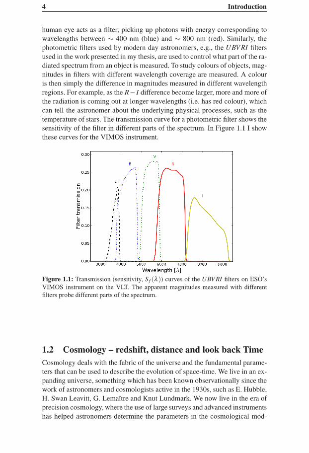
human eye acts as a filter, picking up photons with energy corresponding towavelengths between ∼ 400 nm (blue) and ∼ 800 nm (red). Similarly, thephotometric filters used by modern day astronomers, e.g., the UBVRI filtersused in the work presented in my thesis, are used to control what part of the ra-diated spectrum from an object is measured. To study colours of objects, mag-nitudes in filters with different wavelength coverage are measured. A colouris then simply the difference in magnitudes measured in different wavelengthregions. For example, as the R− I difference become larger, more and more ofthe radiation is coming out at longer wavelengths (i.e. has red colour), whichcan tell the astronomer about the underlying physical processes, such as thetemperature of stars. The transmission curve for a photometric filter shows thesensitivity of the filter in different parts of the spectrum. In Figure 1.1 I showthese curves for the VIMOS instrument.

Figure 1.1: Transmission (sensitivity, S f (λ )) curves of the UBVRI filters on ESO’sVIMOS instrument on the VLT. The apparent magnitudes measured with differentfilters probe different parts of the spectrum.

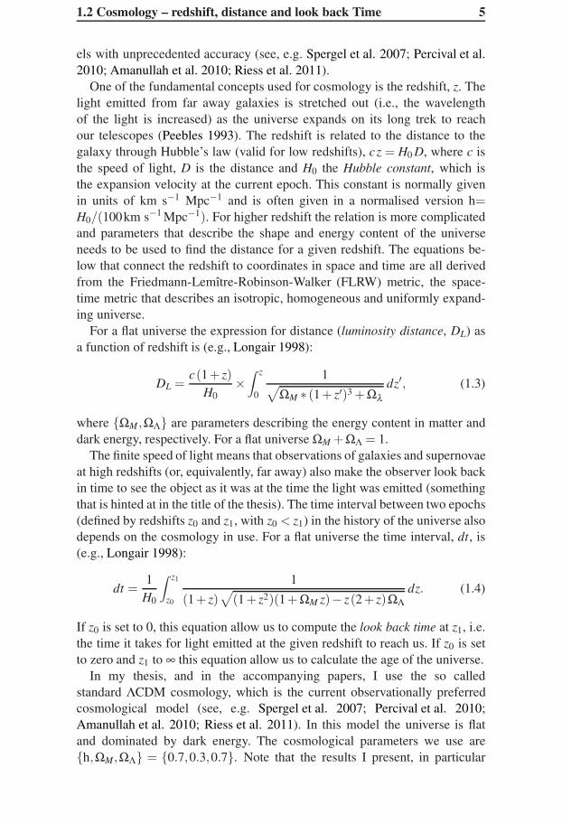
1.2 Cosmology – redshift, distance and look back TimeCosmology deals with the fabric of the universe and the fundamental parame-ters that can be used to describe the evolution of space-time. We live in an ex-panding universe, something which has been known observationally since thework of astronomers and cosmologists active in the 1930s, such as E. Hubble,H. Swan Leavitt, G. Lemaître and Knut Lundmark. We now live in the era ofprecision cosmology, where the use of large surveys and advanced instrumentshas helped astronomers determine the parameters in the cosmological mod-

1.2 Cosmology – redshift, distance and look back Time 5

els with unprecedented accuracy (see, e.g. Spergel et al. 2007; Percival et al.2010; Amanullah et al. 2010; Riess et al. 2011).

One of the fundamental concepts used for cosmology is the redshift, z. Thelight emitted from far away galaxies is stretched out (i.e., the wavelengthof the light is increased) as the universe expands on its long trek to reachour telescopes (Peebles 1993). The redshift is related to the distance to thegalaxy through Hubble’s law (valid for low redshifts), cz = H0 D, where c isthe speed of light, D is the distance and H0 the Hubble constant, which isthe expansion velocity at the current epoch. This constant is normally givenin units of km s−1 Mpc−1 and is often given in a normalised version h=H0/(100km s−1 Mpc−1). For higher redshift the relation is more complicatedand parameters that describe the shape and energy content of the universeneeds to be used to find the distance for a given redshift. The equations be-low that connect the redshift to coordinates in space and time are all derivedfrom the Friedmann-Lemître-Robinson-Walker (FLRW) metric, the space-time metric that describes an isotropic, homogeneous and uniformly expand-ing universe.

For a flat universe the expression for distance (luminosity distance, DL) asa function of redshift is (e.g., Longair 1998):

DL =c(1+ z)

H0×

∫ z

0

1√

ΩM ∗ (1+ z′)3 +Ωλ

dz′, (1.3)

where ΩM ,ΩΛ are parameters describing the energy content in matter anddark energy, respectively. For a flat universe ΩM +ΩΛ = 1.

The finite speed of light means that observations of galaxies and supernovaeat high redshifts (or, equivalently, far away) also make the observer look backin time to see the object as it was at the time the light was emitted (somethingthat is hinted at in the title of the thesis). The time interval between two epochs(defined by redshifts z0 and z1, with z0 < z1) in the history of the universe alsodepends on the cosmology in use. For a flat universe the time interval, dt, is(e.g., Longair 1998):

dt =1

H0

∫ z1

z0

1

(1+ z)√

(1+ z2)(1+ΩM z)− z(2+ z)ΩΛ

dz. (1.4)

If z0 is set to 0, this equation allow us to compute the look back time at z1, i.e.the time it takes for light emitted at the given redshift to reach us. If z0 is setto zero and z1 to ∞ this equation allow us to calculate the age of the universe.

In my thesis, and in the accompanying papers, I use the so calledstandard ΛCDM cosmology, which is the current observationally preferredcosmological model (see, e.g. Spergel et al. 2007; Percival et al. 2010;Amanullah et al. 2010; Riess et al. 2011). In this model the universe is flatand dominated by dark energy. The cosmological parameters we use areh,ΩM,ΩΛ = 0.7,0.3,0.7. Note that the results I present, in particular

6 Introduction

the supernova rates, are easily converted to a different set of cosmologicalparameters. The dependence on h is explicitly stated in the units for the rates.The dependence of ΩM and ΩΛ on supernova rates is not as strong (Pain et al.2002).

7

2 Supernova physics — a briefreview

In this chapter I give a brief introduction to the physics of supernovae and theimplications on the evolution of supernova brightness with time (also knowas the SN light curve). It is believed that supernovae have two different as-trophysical origins, one being the explosion resulting from the gravitationalcollapse of a massive star that has run out of fuel (core collapse), and the othera white dwarf that becomes unstable due to mass accretion from a compan-ion (thermonuclear). Both of these types output extreme amounts of energy,the total amount of visible radiation from both types contain on the order of1044 joules (e.g., Woosley & Janka 2005; Khokhlov et al. 1993). For core col-lapse supernovae this energy is only about one percent of the total energy letloose in the explosion, since almost all of the energy is emitted in the form ofneutrinos.

For both types of supernovae, the decay of radioactive elements (formedduring the explosion) makes an important contribution to the luminosity (e.g.,Leibundgut & Suntzeff 2003). The major contributor is 56Ni, which is themost common radioactive product of nucleosynthesis in supernova explosions(due to being preferred at the nuclear statistical equilibrium present in SNe).The 56Ni decays rather quickly (half-life of ∼6 days) into 56Co which thendecays at a slower pace (half-life of ∼77 days). In the decay process gamma-photons are emitted, they are not able to escape but are absorbed and de-posit energy into the ejecta (but see also Section 2.1.2). That energy will lateremerge as radiation in the optical (or near-IR).

In Papers II and IV we use template light curves to type and to simulatesupernova observations. As examples of how the light curves for the differentsubtypes look like I show our set of template light curves (in the R filter atz = 0.5) in Figure 2.1.

2.1 Core collapse supernovaeAs a massive star reaches the end of its life, having gone through a number ofphases and burning different fuels, the core is made entirely out of iron. Ironis the most stable element, which means that no further chemical reactions(burning) can take place that produces energy. When all of the nuclear fuelin the core have been used up, the gravitational forces are no longer held in

8 Supernova physics — a brief review

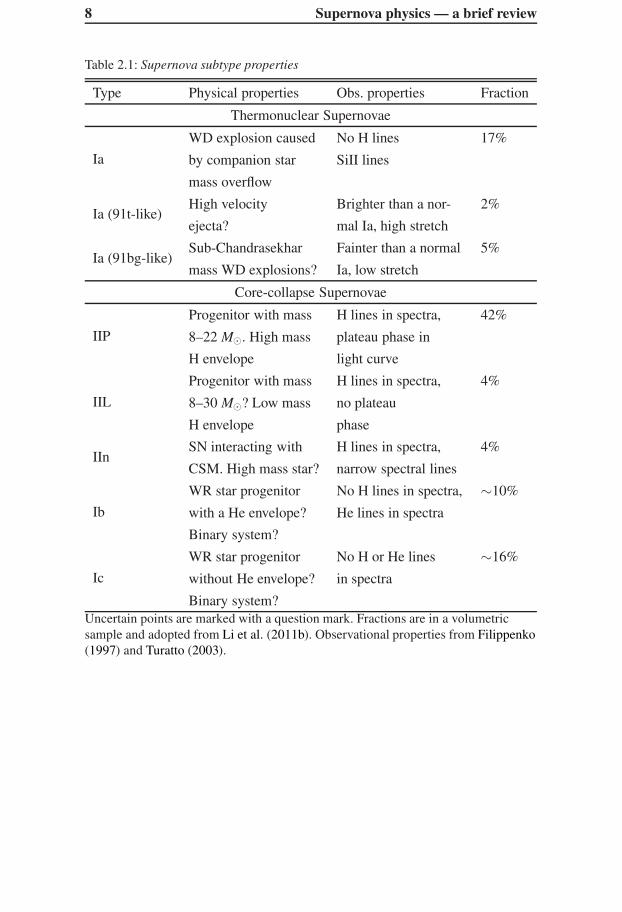
Table 2.1: Supernova subtype properties

Type Physical properties Obs. properties Fraction

Thermonuclear Supernovae

Ia

WD explosion caused No H lines 17%

by companion star SiII lines

mass overflow

Ia (91t-like)High velocity Brighter than a nor- 2%

ejecta? mal Ia, high stretch

Ia (91bg-like)Sub-Chandrasekhar Fainter than a normal 5%

mass WD explosions? Ia, low stretch

Core-collapse Supernovae

IIP

Progenitor with mass H lines in spectra, 42%

8–22 M⊙. High mass plateau phase in

H envelope light curve

IIL

Progenitor with mass H lines in spectra, 4%

8–30 M⊙? Low mass no plateau

H envelope phase

IInSN interacting with H lines in spectra, 4%

CSM. High mass star? narrow spectral lines

Ib

WR star progenitor No H lines in spectra, ∼10%

with a He envelope? He lines in spectra

Binary system?

Ic

WR star progenitor No H or He lines ∼16%

without He envelope? in spectra

Binary system?Uncertain points are marked with a question mark. Fractions are in a volumetricsample and adopted from Li et al. (2011b). Observational properties from Filippenko(1997) and Turatto (2003).

2.1 Core collapse supernovae 9

check by radiation pressure outwards from the produced energy, and the coreof the star collapses. This collapse in the core proceeds rapidly, only about0.1 seconds after the collapse started it is halted, and reversed, when the coreis compressed to the limits set by the nuclear matter. This process is calledshock bounce, the shock that races outwards through the star is what drivesthe supernova (e.g., Janka et al. 2007; Woosley et al. 2002).

If the shock is strong enough to continue through the outer layers in thestar the explosion is known as a “prompt mechanism”. Detailed simulationsof the explosions have problems to make this mechanism work, the shockenergies are just too low to burn through all of the envelope, i.e. the avail-able energy in the shock is not enough to photo-dissociate the iron core. Theexplosion thus stalls before it has propagated through the core. Instead it is be-lieved that the explosion is partly driven by neutrinos, an idea introduced byColgate & White (1966) and revived by Bethe & Wilson (1985). In the cur-rently favoured model, the “delayed neutrino-heating mechanism” neutrinosoriginating from the compact core during the gravitational collapse revive theshock after it stalled in the outer layers (e.g., Janka et al. 2007). The shockthen proceeds through the star and the supernova explosion becomes opticallydetectable when it reaches the surface of the star.

Shock break-out occurs when the shock front reaches the surface ofthe star. This produces an early, extremely bright peak in the SN lightcurve that lasts for a short time (on the order of hours to a few days). Thebrightness of the shock break-out mainly depends on the progenitor size (e.g.Leibundgut & Suntzeff 2003), the smaller the star is the higher the effectivetemperature in the shock and the brighter the break-out becomes. After thebreak-out the photosphere rapidly cools down and the luminosity drops.The luminosity then starts to increase again and reaches a peak at around15–20 days after explosion (e.g. Blinnikov & Bartunov 1993). The increasein luminosity is due to that the photosphere moves physically outwards,increasing the emitting area and thereby also the brightness (and causingthe temperature to fall, making the colour of the supernova redder). This isalso known as the diffusion phase, the evolution depends on the diffusiontime scale (td ∼ M/R, M and R being the mass and radius of the envelope)and how it compares to the the expansion time scale (t ∼ R/V , with V theshock velocity). As the ejecta expands the diffusion time decreases while theexpansion time scale increases, when they are equal the radiation can escape.

At late times the light curve luminosity comes from the decay of radioactiveelements for all but the Ib/c supernovae. As almost all of the 56Ni has decayedinto 56Co at this time, the half-life of the 56Co is 77 days compared to 6 forthe 56Ni decay, the evolution of the light curve is given by the 56Co decay. Thebrightness of the supernova in these late epochs can be used to estimate thetotal mass of 56Ni produced (e.g., Sollerman et al. 1998).

Since massive stars are short-lived compared to the cosmic timescales thecore collapse supernovae trace active star formation. By averaging the CC


SN rate over cosmic volume the current star formation in that volume can bestudied. I will come back to this subject in Chapter 5.

Depending on the mass, and to some extent the surrounding gas content, ofthe progenitor star the observed events looks fairly different, both in terms ofspectra and light curves.

2.1.1 IIP and IIL supernovae

The IIP and IIL subtype of core collapse supernovae are the most commonevents. They originate in a star which has hydrogen left in its envelope asit explodes, their spectra thus contains strong hydrogen lines. The presenceof hydrogen in the spectra was the basis for the original type I/II division(Minkowski 1941). Since stars with masses& 22−30M⊙1 (Maeder & Meynet2010) are believed to have shed their hydrogen envelopes prior to the explo-sion the progenitor stars of IIP/L supernovae are thought to be less massivethan this. Smartt (2009) review the current status of progenitor studies, thereported lower mass limit based on observations is 8.5+1.5

−1.0. This limit is foundto match the theoretical limit of ∼ 9M⊙ quite well.

The spectra from IIP and IIL supernovae are similar, making it all but im-possible to distinguish between them with spectral information only. However,they have very different light curves, with IIP SNe showing a characteristicplateau phase reaching from ∼10 to ∼ 100 days after explosion, and IIL SNeshowing a linear decline. The plateau phase is the result of hydrogen recom-bination taking place in the hydrogen envelope after shock break-out (Popov1993). The recombination front moves inward in the ejecta, but staying ata constant absolute radius. The constant radius, combined with the constanttemperature given by the recombination (∼ 5000 K), is what causes the lu-minosity of the supernova to be constant in the plateau phase. This phaseends when the recombination front has passed through the entire hydrogenenvelope. The light curve shape is then determined by radioactive decay asdescribed above.

The plateau phase is notably absent in IIL SNe, this is believed to be dueto them having a much smaller hydrogen envelope (e.g., Smartt 2009), whichwill go through recombination very fast, before a real recombination front hasformed properly. There are some indications that the progenitors of IIL SNeare more massive than IIP progenitors on average. The more massive corecollapse progenitors would, in this picture, have shed most of their hydrogenbefore the explosion (e.g., Smartt 2009). It should also be noted that IIL SNeare very rare events, only about one in thirty supernovae are expected to be ofthis kind in a volume-limited (i.e., all SNe within a given volume are found)sample (Li et al. 2011b).

1M⊙ is the mass of the Sun.

2.1 Core collapse supernovae 11

2.1.2 Ib and Ic supernovae

These supernova types are both believed to originate from Wolf-Rayet (WR)stars (e.g., Gaskell et al. 1986; Maeder & Meynet 2010). WR stars are massive(&20 M⊙), rotating stars that have very strong stellar winds. These windscause them to lose a lot of mass (Crowther 2007). The outer layers of the staris thus lost, which means that the hydrogen envelope is missing for WR starsof the lower mass range, and that both the hydrogen and helium envelope aremissing for the more massive ones. This is then thought to be the explanationto why these spectral lines are absent from the spectra of Ib (H missing) andIc (H and He missing) SNe.

There is growing support for another possible formation channel for IbcSNe. Nomoto et al. (1995) suggested that a lower mass binary system mayform Ibc supernovae. In this theory the star that later explodes as SN loses itsH/He envelope to the binary companion via Roche lobe overflow.

The light curves of Ib and Ic supernovae are quite similar; in our work,where focus is on the light curves, we have used the joint class Ibc SNe todescribe both populations. The plateau phase of IIP SNe is not present in IbcSNe, due to the lack of a H envelope. The curves are instead dominated bythe diffusion of the thermal shock and radioactive decay. At late times thelight curves of these SNe are steeper than the type IIs. This is believed to bedue to escape of gamma photons from the radioactive decay, i.e. not all of theavailable energy from the decay is absorbed and re-emitted as optical radiation(e.g., Leibundgut & Suntzeff 2003).

2.1.3 IIn supernovae

The IIn SNe is a subset of core collapse supernovae with narrowspectral lines and a somewhat slower evolution (e.g, Fransson et al. 2002;Leibundgut & Suntzeff 2003). They can be very bright at peak and canalso stay bright for a longer time period than the normal supernova modelwould allow. The most probably explanation is that they are SNe where theshock front has interacted with the surrounding circumstellar material (CSM,material that has been lost by star during its evolution). As the shock frontcontinues outside the stellar envelope after shock break-out it will run into theCSM, and further conversion of the kinetic energy in the shock into radiationtakes place. This provides the additional energy source that is required toexplain the brightness and slower light curve. The narrow lines are believedto originate from gas in the CSM, since these gas clouds move slower thanthe ejecta the lines will look narrow in comparison. Also, the line strengthsand ratios of the narrow lines indicate that they originate from clouds withhigh density, making the CSM a more likely source than interstellar matter(Fransson et al. 2002).


Figure 2.1: This figure contains example light curves for different supernova types.Note that these are R filter light curves at z ∼ 0.5, which corresponds to rest-frame B atthat redshift. The shift to higher z also stretch the curves by a factor (1+z). Also, theseare template light curves based on the average of many supernovae, a real individualSN light curve will often be less smooth than these examples.

The light curves of IIn SNe are quite varied. Due to the importance of lineemission from the interaction with the CSM, the resulting light curves andpeak luminosity can be very different (e.g. Leibundgut & Suntzeff 2003).

2.2 Thermonuclear supernovaeSupernovae resulting from thermonuclear explosions are in general more uni-form than the core collapse. This is due to the origin of the explosion. Inthese SNe the progenitor is a compact star that explodes. The most likely typeof compact object is a white dwarf since they consist of mainly carbon andoxygen which provides fuel for the explosion (e.g., Leibundgut 2000). In thispicture the detonation sets as the white dwarf has increased its mass beyondthe Chandrasekhar mass limit (the theoretical mass limit for white dwarfs, seeChandrasekhar 1934) by accreting matter from a companion.

The exact nature of the explosion is not well constrained currently. Oneof the many proposed ideas is the “delayed detonation model” (Hoflich et al.1995) in which the burning starts as a deflagration (subsonic burning) andlater on changes to a detonation (supersonic burning, causing a shock frontto form). Another idea is that the explosion occurs below the Chandrasekharlimit (so called sub-Chandrasekhar mass white dwarfs) and starts at the bottom

2.2 Thermonuclear supernovae 13

of the He surface layer in the white dwarf (e.g., Nomoto 1982; Leibundgut2000). It is also possible that Ia supernovae can come from many differentexplosion (and progenitor) channels.

The nature of the companion is not known, the two competing models arethe “double degenerate” (DD) scenario, where the companion is another whitedwarf; and the “single degenerate” (SD) scenario, in which the companion ismain sequence, or further evolved, star. In the SD scenario the lack of hydro-gen and helium in the Ia spectra is explained by the white dwarf accretingand burning this material before becoming a SNe. In the DD theory, the whitedwarfs merge after losing orbital energy in the form of gravitational radiation(Leibundgut 2000).

The spectra of Ia supernovae are characterised by SiII lines at early times.The presence of these lines, and absence of H or He lines, is used to type theSNe spectroscopically (Filippenko 1997). The light curves are completely de-termined by the decay of radioactive elements. As for core collapse SNe, thelight curve shape is formed as a race between diffusion and expansion (seeSection 2.1). The general shape of the light curve (how fast it is) has beenfound to correlate to the peak brightness (Phillips et al. 1999). This feature,also known as stretch is used in supernova cosmology experiments to “stan-dardise” (i.e. reducing the scatter of observable luminosity) the Ia supernovabrightness. The stretch of a light curve is proportional to the peak brightness,i.e. the faster the light curve decays, the fainter peak.

Despite the uniformity of Ia SNe, exceptions do exist. SN 1991T (and otherIa’s similar to this) was a very bright Ia SNe, which also had a somewhat dif-ferent spectral evolution than normal Ia SNe in that the SiII lines appearedlater than normal (Filippenko et al. 1992b). At the other end of the luminos-ity range is SN 1991bg (and similar SNe), which was a sub-luminous Ia su-pernovae with peculiar spectral features (Filippenko et al. 1992a). It is possi-ble that the faint 91bg-like SNe originate from sub-Chandrasekhar mass whitedwarfs (Stritzinger et al. 2006).

In Chapter 5 I describe how the Ia supernova rates can be used to put con-straints on the progenitor system. Depending on the type of companion and thephysics of the merging/accretion the time from the formation of the progenitorstar to Ia explosion can be wildly different. This time scale, the so called de-

lay time, can be studied with Ia rate measurements (e.g., Ruiz-Lapuente et al.1995).

15

3 Detecting supernovae and galaxiesat high redshift

3.1 The Stockholm VIMOS Supernova SearchThe main research project I have worked on during my time as graduate stu-dent and also the main focus of this thesis is the The Stockholm VIMOS Su-pernova Search (SVISS). The data for the project were obtained with the VI-MOS instrument (LeFevre et al. 2003), mounted on the ESO Very Large Tele-scope (Unit Telescope 3), at several epochs during 2003–2006. The VIMOSinstrument has four CCDs, each 2k×2.4k pixels with a pixel scale of 0.205arcsec/pxl, covering a total area of 4×56 sq. arcmin. The SVISS observationswere obtained in two fields, covering parts of the Chandra Deep Field-South(Giacconi et al. 2001) and the ELAIS-S1 field (La Franca et al. 2004). The ob-servations in the ELAIS-S1 field were obtained in five broad band filters (U ,B, V , R and I). The data used in the papers included in this thesis are only fromthe ELAIS-S1 observations, the CDF-S results are yet to be published.

The supernova search was conducted in the R and I filters. The observa-tions in these filters were divided into seven search epochs with one month inbetween (taken in the autumn of 2004) and one reference epoch from obser-vations obtained approximately one year earlier. We also obtained a controlepoch, one year after the last search epoch. The image quality for these ob-servations was overall very good, the mean seeing of the epochs and filters isroughly 0.7 arcseconds. In Paper II we give details on the data for the differentepochs.

The observations are also very deep, with mean 3σ limiting magnitudesof 26.8 and 26.3 in R and I, respectively. Comparing these magnitudes tothe limits given by other surveys (Dahlen et al. 2008; Morokuma et al. 2008;Totani et al. 2008), we find that our data set is among the deepest ever obtained(for supernova searching), although smaller in field size.

The UBV observations were obtained at several different occasions duringthe time period 2004-2006. Details on the data reduction and calibration of theUBV data along with a galaxy catalogue for the field is presented in Paper III.For the supernova part of the survey the UBV observations have only beenused to calculate photometric redshifts for supernova host galaxies.

16 Detecting supernovae and galaxies at high redshift

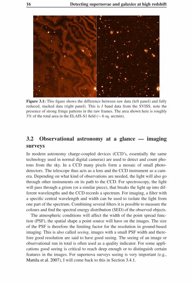
Figure 3.1: This figure shows the difference between raw data (left panel) and fullyreduced, stacked data (right panel). This is I band data from the SVISS, note thepresence of strong fringe patterns in the raw frames. The area shown here is roughly3% of the total area in the ELAIS-S1 field (∼ 6 sq. arcmin).

3.2 Observational astronomy at a glance — imagingsurveysIn modern astronomy charge-coupled devices (CCD’s, essentially the sametechnology used in normal digital cameras) are used to detect and count pho-tons from the sky. In a CCD many pixels form a mosaic of small photo-detectors. The telescope thus acts as a lens and the CCD instrument as a cam-era. Depending on what kind of observations are needed, the light will also gothrough other instruments on its path to the CCD. For spectroscopy, the lightwill pass through a grism (or a similar piece), that breaks the light up into dif-ferent wavelengths and the CCD records a spectrum. For imaging, a filter witha specific central wavelength and width can be used to isolate the light fromone part of the spectrum. Combining several filters it is possible to measure thecolours and find the spectral energy distribution (SED) of the observed objects.

The atmospheric conditions will affect the width of the point spread func-tion (PSF), the spatial shape a point source will have on the images. The sizeof the PSF is therefore the limiting factor for the resolution in ground-basedimaging. This is also called seeing, images with a small PSF width and there-fore good resolution are said to have good seeing. The seeing of an image orobservational run in total is often used as a quality indicator. For some appli-cations good seeing is critical to reach deep enough or to distinguish certainfeatures in the images. For supernova surveys seeing is very important (e.g.,Mattila et al. 2007), I will come back to this in Section 3.4.1.

3.2 Observational astronomy at a glance — imaging surveys 17

In imaging surveys the telescope is used to observe a patch on the skyinstead of a specific object. The resulting images can contain thousands uponthousands of objects, galaxies and stars. The larger the field-of-view the moresources can be found. By observing in multiple filters, colour informationbecomes available for the objects and can be used to characterise the objectstogether with their brightness. Due to limitations in available observation timeand instrumentation, most surveys up till now have been either deep — depthrefers to the distance at which sources can be detected — but covering a smallfield (i.e. a pencil-beam survey) or shallow but covering a large field. To reacheven the faintest high redshift galaxies, depth is the most important parameter.Some of the deepest and most successful surveys when it comes to studyinghigh redshift galaxies are the Ultra Deep Field (UDF, Beckwith et al. 2006),the Great Observatories Origins Deep Survey (GOODS, Giavalisco et al.2004b), the Cosmological Evolution Survey (COSMOS, Koekemoer et al.2007) and the Subaru Deep Field (SDF, Kashikawa et al. 2004). Surveystargetting huge areas on the sky are by necessity (the observational time limitsmentioned above) more shallow. Examples of such surveys are the SloanDigital Sky Survey (SDSS, Abazajian et al. 2009), the 2dF Galaxy RedshiftSurvey (2dFGRS, Colless et al. 2001) and the Two Micron All Sky Survey(2MASS, Jarrett et al. 2000).

3.2.1 Image data reduction

The raw image files from the telescope have to be properly calibrated andcleaned, a process called reduction. For broad band imaging of the type usedin SVISS normal image reduction consists of the following steps. The imagesare debiased, removing the signal from the instrument itself that is presenteven in images with zero exposure time. Any variations in sensitivity over theCCD is corrected for by flatfielding the data, using observations of a uniformlyilluminated surface (such as a white screen or the twilight sky). Cosmic ray re-jection routines are used to remove any image artifacts resulting from cosmicparticles hitting the CCD. Corrections for atmospheric extinction can also bedone at this point. To avoid saturating the CCD observations during a singlenight is normally divided into several exposures. The final step of the reductionprocess is thus to first align the images to a common pixel coordinate systemand then to combine, or stack, the individual images. The resulting stacked im-ages are then calibrated by comparing to observations of photometric standardstars, with well-known photometry, using the same instrumental setup.

For SVISS we did all of the reductions in the ESO-MIDAS1 system us-ing a set of scripts written for this particular data set. In Papers II and IIIwe presented details on how the reductions were done for the supernova andgalaxy part of the survey, respectively. Photometric calibration was done in

1see http://www.eso.org/sci/software/esomidas/midas-overview.html

http://www.eso.org/sci/software/esomidas/midas-overview.html


PYRAF/IRAF (Tody 1986) using the photcal package. Figure 3.1 showsthe effect of data reduction and stacking on the observations.

The VIMOS I band suffers from rather severe effects of fringing (seeBerta et al. 2008, for a detailed description of fringing for the VIMOSinstrument), this is essentially optical interference patterns formed in the thinCCD layers. For the SVISS we constructed a fringe map for each observationnight by median combining the images taken during that night and rejectingbright pixels by a standard sigma-rejection routine. To make this possible theobservations were done using many different, slightly offset, positions andtaking multiple images. This scheme was optimised to avoid having individualimages target the same area on sky. The fringe map was then subtracted fromeach of the images, before stacking, which successfully removed the patterns.

In Paper III we investigated how different choices on how to combine theimages affects the output data quality. We found that the best option (at least forthe SVISS data set) was to use a weighted average method, where the weightswere given by the inverse of the PSF width, i.e. images with good seeing havegreater weight than bad seeing images. Stacked images were produced for eachfilter and epoch for the supernova search. We also created deep images bystacking all of the good quality frames in each filter. These images were usedfor the galaxy survey part of the project.

3.2.2 Source detection and photometry

The detection of sources in images from modern astronomical surveys can nor-mally not be done manually, to consistently find faint objects above a certainsignal-to-noise level, specialised computer codes are used. For the work pre-sented in this thesis we used the publicly available software Source Extractor(SE Bertin & Arnouts 1996) to find both galaxies and supernovae. This code isa standard tool used for imaging surveys. For an extended manual please referto Holwerda (2005), this report also contains several examples of SE use in theliterature. In Papers II and III we describe the way SE has been used to de-tect supernovae in the epoch images and galaxies in the fully stacked images,respectively.

For reference I now give a brief overview on how SE detects sources. First,the mean background intensity and noise level in the image is estimated. Thisbackground intensity is then removed from the image and the software flagspixels as detected if they are over a user-specified threshold. It then removesall detected pixels that belong to a connected region smaller than another user-specified threshold. At this point some of the detected objects will containmany sources that are so close to each other that their detected regions overlap.The program then tries to deblend the objects into the individual sources, byusing contrast settings set by the user. The deblended source list can be furtherprocessed but is more or less the final output.

3.3 Studying galaxies with surveys 19

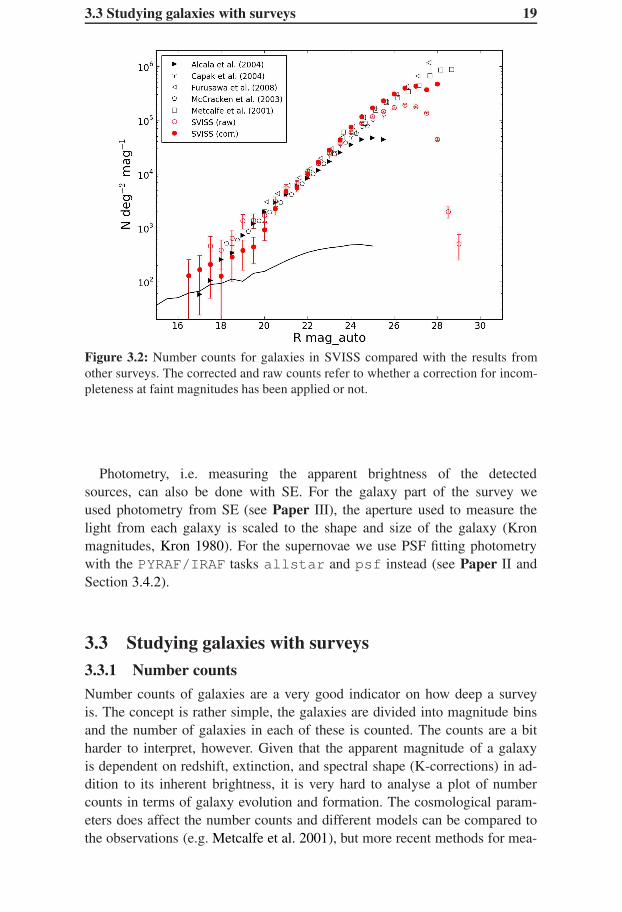
Figure 3.2: Number counts for galaxies in SVISS compared with the results fromother surveys. The corrected and raw counts refer to whether a correction for incom-pleteness at faint magnitudes has been applied or not.

Photometry, i.e. measuring the apparent brightness of the detectedsources, can also be done with SE. For the galaxy part of the survey weused photometry from SE (see Paper III), the aperture used to measure thelight from each galaxy is scaled to the shape and size of the galaxy (Kronmagnitudes, Kron 1980). For the supernovae we use PSF fitting photometrywith the PYRAF/IRAF tasks allstar and psf instead (see Paper II andSection 3.4.2).

3.3 Studying galaxies with surveys

3.3.1 Number counts

Number counts of galaxies are a very good indicator on how deep a surveyis. The concept is rather simple, the galaxies are divided into magnitude binsand the number of galaxies in each of these is counted. The counts are a bitharder to interpret, however. Given that the apparent magnitude of a galaxyis dependent on redshift, extinction, and spectral shape (K-corrections) in ad-dition to its inherent brightness, it is very hard to analyse a plot of numbercounts in terms of galaxy evolution and formation. The cosmological param-eters does affect the number counts and different models can be compared tothe observations (e.g. Metcalfe et al. 2001), but more recent methods for mea-


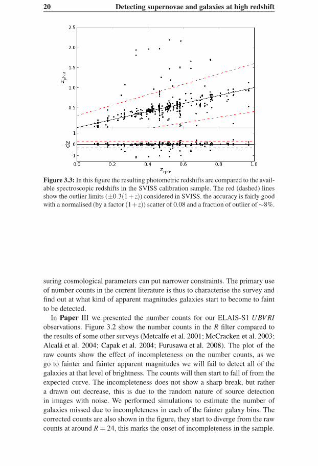
Figure 3.3: In this figure the resulting photometric redshifts are compared to the avail-able spectroscopic redshifts in the SVISS calibration sample. The red (dashed) linesshow the outlier limits (±0.3(1+ z)) considered in SVISS. the accuracy is fairly goodwith a normalised (by a factor (1+z)) scatter of 0.08 and a fraction of outlier of ∼8%.

suring cosmological parameters can put narrower constraints. The primary useof number counts in the current literature is thus to characterise the survey andfind out at what kind of apparent magnitudes galaxies start to become to faintto be detected.

In Paper III we presented the number counts for our ELAIS-S1 UBV RI

observations. Figure 3.2 show the number counts in the R filter compared tothe results of some other surveys (Metcalfe et al. 2001; McCracken et al. 2003;Alcalá et al. 2004; Capak et al. 2004; Furusawa et al. 2008). The plot of theraw counts show the effect of incompleteness on the number counts, as wego to fainter and fainter apparent magnitudes we will fail to detect all of thegalaxies at that level of brightness. The counts will then start to fall of from theexpected curve. The incompleteness does not show a sharp break, but rathera drawn out decrease, this is due to the random nature of source detectionin images with noise. We performed simulations to estimate the number ofgalaxies missed due to incompleteness in each of the fainter galaxy bins. Thecorrected counts are also shown in the figure, they start to diverge from the rawcounts at around R = 24, this marks the onset of incompleteness in the sample.

3.3 Studying galaxies with surveys 21

3.3.2 Photometric redshifts

The redshift of galaxies is normally determined by matching the observedspectral lines to their rest-frame counterparts. In this way very accurateredshift measurements can be made. But the observational costs of obtainingspectra for many faint galaxies are huge, thus another approach is often usedfor galaxy surveys. The solution is to use so called photometric redshifttechniques which have been used extensively since the first attempts some 25years ago (Loh & Spillar 1986) . With this technique, photometry in a numberof broad band filters (e.g. UBV RI) is used to find the redshift of the galaxy.The two main photometric redshift methods are the empirical training setmethod, e.g., ANNz (Collister & Lahav 2004); MLP (Vanzella et al. 2004);ArborZ Gerdes et al. (2010) and the template fitting method, e.g., HyperZ(Bolzonella et al. 2000); BPZ (Benítez 2000); ZEBRA (Feldmann et al.2006). Hildebrandt et al. (2008) compare the different codes and find that thephotometric redshift accuracy reached by them is reasonable, but that the errorestimates for individual galaxies are not believable. Photometric redshifts arethus better suited to obtaining redshifts for entire galaxy populations than forindividual systems.

In the empirical training set method the goal is to find the relation betweencolours and redshift by using galaxies for which a spectroscopic redshift hasbeen determined, then the colours of galaxies with unknown redshift can bemapped onto the relation and the redshifts found. To reach good accuraciesthis method needs a large training set of galaxies with spectroscopic redshifts,making it less suited for high redshift studies (Benítez 2000). The template fit-ting method instead uses a library of spectral energy distributions for differentgalaxy types that are redshifted. The colours of the template SEDs are thenmatched to the observed colours and the the best-fitting redshift (and template)is chosen to be the correct one.

The photometric redshifts calculated in Paper III and used in Papers II andIV were obtained using the GOODSZ code (Dahlen et al. 2010). This code isa hybrid between the template and empirical methods. While it uses templatesand χ2 fitting to find the correct redshift, the code can also be trained by run-ning it on galaxies with known spectroscopic redshifts. In Paper III detailson the training of GOODSZ as applied to the SVISS data set are given. InFigure 3.3 I show the accuracy of the photometric redshifts for z < 1 for ourcalibration set of galaxies. It should be noted that the lack of observations inthe near-infrared (i.e. red-wards of the I filter) causes the photometric redshiftsto become very uncertain beyond z ∼ 1.

3.3.3 Lyman break galaxies

Lyman Break Galaxies (LBGs) are star forming galaxies at high redshift (seeGiavalisco 2002, for an extensive review). The spectra of star forming galaxiesexhibit a strong break at the rest-frame wavelength of the Lyman limit (at 91.2


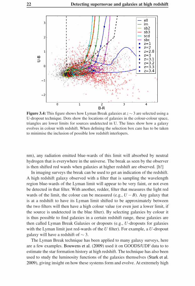
Figure 3.4: This figure shows how Lyman Break galaxies at z ∼ 3 are selected using aU-dropout technique. Dots show the locations of galaxies in the colour-colour space,triangles are lower limits for sources undetected in U. The lines show how a galaxyevolves in colour with redshift. When defining the selection box care has to be takento minimise the inclusion of possible low redshift interlopers.

nm), any radiation emitted blue-wards of this limit will absorbed by neutralhydrogen that is everywhere in the universe. The break as seen by the observeris then shifted red wards when galaxies at higher redshift are observed. [h!]

In imaging surveys the break can be used to get an indication of the redshift.A high redshift galaxy observed with a filter that is sampling the wavelengthregion blue-wards of the Lyman limit will appear to be very faint, or not evenbe detected in that filter. With another, redder, filter that measures the light redwards of the limit, the colour can be measured (e.g., U −B). Any galaxy thatis at a redshift to have its Lyman limit shifted to be approximately betweenthe two filters will then have a high colour value (or even just a lower limit, ifthe source is undetected in the blue filter). By selecting galaxies by colour itis thus possible to find galaxies in a certain redshift range, these galaxies arethen called Lyman Break Galaxies or dropouts (e.g., U -dropouts for galaxieswith the Lyman limit just red-wards of the U filter). For example, a U -dropoutgalaxy will have a redshift of ∼ 3.

The Lyman Break technique has been applied to many galaxy surveys, hereare a few examples. Bouwens et al. (2009) used it on GOODS/UDF data to toestimate the star formation history at high redshift. The technique has also beenused to study the luminosity functions of the galaxies themselves (Stark et al.2009), giving insight on how these systems form and evolve. At extremely high

3.4 How to find supernovae 23

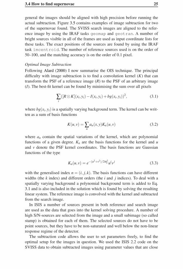
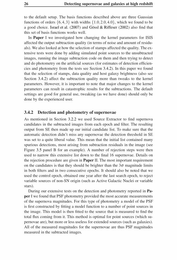
Figure 3.5: Example images of two supernovae found by the SVISS. The upper panel(A) and lower panel (B) show image cutouts for SN357 and SN115, respectively. Theleftmost images are RGB colour composites using the supernova peak epoch for thered channel and deep B and V images for the blue and green channels. The middleimages show the reference epoch in I and the images to the right the subtracted I

band image. The red cross indicates the position of the supernova. In panel B, notethe presence of a subtraction residual in the subtracted image (in the topmost rightcorner).

redshifts (with dropout filters in the near infrared), Bunker et al. (2010) haveestimated the contribution of LBGs to the cosmic reionization.

Our LBG selection criteria and the resulting sample is presented in Pa-per III. The criteria for the U -dropouts are shown in Figure 3.4, sources thathave colours (or lower limits on the colours) placing them inside the selectionbox are considered to be LBGs at z ∼ 3. The U dropout selection is found to bequite secure and the resulting sample is among the deepest ever observed. Inthe paper we also present B and V -dropouts, these samples are less secure sincethey are contaminated by low redshift interlopers that have colours similar tothe high redshift galaxies.

3.4 How to find supernovae

3.4.1 Image subtraction

Supernovae are not always easily found. It is only rarely that a SN will out-shine its host galaxy (as alluded to in Chapter 1), in most cases the supernovalight will be a small part of light measured from the galaxy. Also, in the case ofground-based observations of high redshift galaxies, the galaxies themselveswill not be fully resolved (see Section 3.2). This means that the SN itself will


be less distinct and easily missed when looking in the individual search epochimages. The solution to this problem is simple in concept, but harder in prac-tice. By subtracting an image from an earlier epoch from the search epochimages the light from the galaxies is removed, leaving the supernovae to befound. The problem with this approach is that the image quality (seeing andnoise level) can vary from epoch to epoch. Any subtraction method must thusbe able to deal with these issues while still producing an output that conservesthe intensities in the input images.

The combination of the atmospheric effects with the optics, focusing andcamera setup results in variations of the seeing in the images both in spatialcoordinates and over time (i.e. different epochs can have different seeing, andalso different spatial variation). A successful image subtraction technique mustbe able to match the PSF of the reference image to the PSF of the later epochimages while also allowing the convolution kernel to vary spatially. The Op-

timal Image Subtraction (OIS) technique presented in Alard & Lupton (1998)and further refined in Alard (2000) allows this. For the SVISS images we haveused the code that implements this technique, ISIS 2.2 (Alard 2000).

Difference imaging, and ISIS in particular, has been used to detect SNein many projects. Many of the large Ia surveys use ISIS (or similar codes)to find SN candidates (e.g. Cappellaro et al. 2005; Wood-Vasey et al. 2007;Poznanski et al. 2007b), then following up with spectroscopic observations ofthe candidates. Cappellaro et al. (2005) and Botticella et al. (2008) used thesame technique in their SN surveys. Difference imaging has also successfullybeen used in near-infrared SN searches (e.g. Maiolino et al. 2002; Mattila et al.2007) concentrating on local luminous infrared galaxies. More recently, dif-ference imaging has also successfully been applied to mid-infrared SN ob-servations with the Spitzer Space Telescope (Meikle et al. 2006). In additionto SN surveys, OIS and ISIS has been used by various authors investigatingmany different subjects, among which are variable stars in crowded fields (e.g.Corwin et al. 2006), gravitational microlensing (e.g. Alard 2001; Sumi et al.2006) and the detection of planets (e.g. Holman et al. 2007).

For the SVISS we constructed a supernova detection pipeline suitable forlarge images and multi-epoch data. The pipeline consists of a number ofIRAF/PYRAF scripts that are run in sequence, and go through the followingsteps: (i) accurate image alignment over the entire frame; (ii) convolving thebetter seeing image to the same PSF size and shape as the poorer seeingimage, using a spatially varying kernel; (iii) subtracting the images. Theinput to the pipeline consists of one reference image and a list of later epochimages.

Aligning Images

The subtraction method is quite sensitive to how well the images are regis-tered. Spatial variability of the convolution kernel can somewhat compensatefor a non-perfect image alignment (also discussed in Israel et al. 2007), but in


general the images should be aligned with high precision before running theactual subtraction. Figure 3.5 contains examples of image subtraction for twoof the supernovae found. The SVISS search images are aligned to the refer-ence image by using the IRAF tasks geomap and geotran. A number ofbright sources visible in all of the frames are used as input coordinate lists forthese tasks. The exact positions of the sources are found by using the IRAFtask imcentroid. The number of reference sources used is on the order of50–100, and the matching accuracy is on the order of 0.1 pixel.

Optimal Image Subtraction

Following Alard (2000) I now summarise the OIS technique. The principaldifficulty with image subtraction is to find a convolution kernel (K) that cantransform the PSF of a reference image (R) to the PSF of an arbitrary image(I). The best-fit kernel can be found by minimising the sum over all pixels

∑i

([R⊗K](xi,yi)− I(xi,yi)+bg(xi,yi))2, (3.1)

where bg(xi,yi) is a spatially varying background term. The kernel can be writ-ten as a sum of basis functions

K(u,v) = ∑n

an(x,y)Kn(u,v) (3.2)

where an contain the spatial variations of the kernel, which are polynomialfunctions of a given degree. Kn are the basis functions for the kernel and u

and v denote the PSF kernel coordinates. The basis functions are Gaussianfunctions of the type

Kn(u,v) = e−(u2+v2)/2σ2k uiv j (3.3)

with the generalised index n = (i, j,k). The basis functions can have differentwidths (the k index) and different orders (the i and j indices). To deal with aspatially varying background a polynomial background term is added to Eq.3.1 and is also included in the solution which is found by solving the resultinglinear system. The reference image is convolved with the kernel and subtractedfrom the search image.

In ISIS a number of sources present in both reference and search imageare used as the data that goes into the kernel solving procedure. A number ofhigh S/N-sources are selected from the image and a small subimage (so calledstamp) is obtained for each of them. The selected sources do not have to bepoint sources, but they have to be non-saturated and well below the non-linearresponse regime of the detector.

The subtraction code allows the user to set parameters freely, to find theoptimal setup for the images in question. We used the ISIS 2.2 code on theSVISS data to obtain subtracted images using parameter values that are close


to the default setup. The basis functions described above are three Gaussianfunctions of orders 6,4,3 with widths 1.0,2.0,4.0, which we found to bea good choice. Israel et al. (2007) and Gössl & Riffeser (2002) also find thatthis set of basis functions works well.

In Paper I we investigated how changing the kernel parameters for ISISaffected the output subtraction quality (in terms of noise and amount of residu-als). We also looked at how the selection of stamps affected the quality. The ex-tensive tests were done by adding simulated point sources to the unsubtractedimages, running the image subtraction code on them and then trying to detectand do photometry on the artificial sources (for estimates of detection efficien-cies and photometry from the tests see Section 3.4.2). In this paper we foundthat the selection of stamps, data quality and host galaxy brightness (also seeSection 3.4.2) affect the subtraction quality more than tweaks to the kernelparameters. However, it is important to note that major changes to the kernelparameters can result in catastrophic results for the subtractions. The defaultsettings are good for general use, tweaking (as we have done) should only bedone by the experienced user.

3.4.2 Detection and photometry of supernovae

As mentioned in Section 3.2.2 we used Source Extractor to find supernovacandidates in the subtracted images from each epoch and filter. The resultingoutput from SE then made up our initial candidate list. To make sure that theautomatic detection didn’t miss any supernovae the detection threshold in SEwas set to a quite liberal value. This mean that the initial list contained manyspurious detections, most arising from subtraction residuals in the image (seeFigure 3.5 panel B for an example). A number of rejection steps were thenused to narrow this extensive list down to the final 16 supernovae. Details onthe rejection procedure are given in Paper II. The most important requirementon the candidates is that they should be brighter than the 3σ magnitude limitsin both filters and in two consecutive epochs. It should also be noted that weused the control epoch, obtained one year after the last search epoch, to rejectvariable sources of non-SN origin (such as Active Galactic Nuclei or variablestars).

During our extensive tests on the detection and photometry reported in Pa-per I we found that PSF photometry provided the most accurate measurementsof the supernova magnitudes. For this type of photometry a model of the PSFis first constructed by fitting a model function to a number of point sources inthe image. This model is then fitted to the source that is measured to find thetotal flux coming from it. This method is optimal for point sources (which su-pernovae are), but more or less useless for extended sources (such as galaxies).All of the measured magnitudes for the supernovae are thus PSF magnitudesmeasured in the subtracted images.


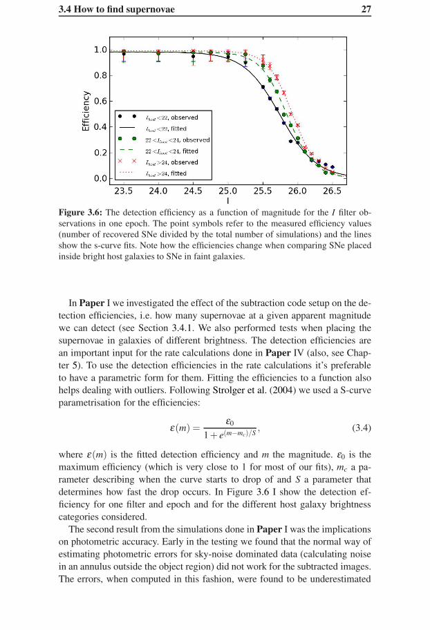
Figure 3.6: The detection efficiency as a function of magnitude for the I filter ob-servations in one epoch. The point symbols refer to the measured efficiency values(number of recovered SNe divided by the total number of simulations) and the linesshow the s-curve fits. Note how the efficiencies change when comparing SNe placedinside bright host galaxies to SNe in faint galaxies.

In Paper I we investigated the effect of the subtraction code setup on the de-tection efficiencies, i.e. how many supernovae at a given apparent magnitudewe can detect (see Section 3.4.1. We also performed tests when placing thesupernovae in galaxies of different brightness. The detection efficiencies arean important input for the rate calculations done in Paper IV (also, see Chap-ter 5). To use the detection efficiencies in the rate calculations it’s preferableto have a parametric form for them. Fitting the efficiencies to a function alsohelps dealing with outliers. Following Strolger et al. (2004) we used a S-curveparametrisation for the efficiencies:

ε(m) =ε0

1+ e(m−mc)/S, (3.4)

where ε(m) is the fitted detection efficiency and m the magnitude. ε0 is themaximum efficiency (which is very close to 1 for most of our fits), mc a pa-rameter describing when the curve starts to drop of and S a parameter thatdetermines how fast the drop occurs. In Figure 3.6 I show the detection ef-ficiency for one filter and epoch and for the different host galaxy brightnesscategories considered.

The second result from the simulations done in Paper I was the implicationson photometric accuracy. Early in the testing we found that the normal way ofestimating photometric errors for sky-noise dominated data (calculating noisein an annulus outside the object region) did not work for the subtracted images.The errors, when computed in this fashion, were found to be underestimated


Figure 3.7: Example light curve and colour evolution for one of the discovered super-novae in the SVISS. The lines show the most probable Bayesian fit (also see Chapter 4and Paper II).

by a factor of two or more. All photometric errors for the supernovae havethus been estimated from the simulations. The scatter in the output photometryfor simulated supernovae of the same magnitude is adopted as the error forSN measurements of the given magnitude. In this paper we also found a smallphotometric bias that affected the supernovae inside galaxies. Again using thesimulations we showed that the photometry could be corrected for this bias.

In Paper II we reported the discovery of 16 supernovae in the SVISSELAIS-S1 observations. These SNe were found by using the method outlinedin this chapter. In Figure 3.7 we show the light curve and colour evolution forone of the discovered supernovae together with a fitted light curve (see nextchapter).

29

4 Photometric Classification ofSupernovae

The classification of supernovae is traditionally done by inspecting the spec-tra and checking for the presence of signature lines (see Chapter 2). However,since spectra are very hard and observationally expensive to obtain for highredshift supernovae, photometric methods where the light curves are used in-stead have become more and more important in supernova surveys. The basicmethodology of photometric typing is to construct template light curves fromempirical or model light curves and spectra for the supernova subtypes andthen to fit these templates to the observed light curves. The big advantage ofthis method is, as alluded to above, that it is far easier to obtain photometryof faint SNe at high redshift than to obtain spectra. The drawback is that thetyping is a lot less secure, there are inherent degeneracies between the lightcurves of different subtypes which can cause the typing to fail, irrespective ofthe method.

4.1 Examples of photometric supernova typing in theliteratureTyping of supernovae using broad band colours in multiple epochs has beendone by several authors. Poznanski et al. (2002), Dahlén & Goobar (2002) andJohnson & Crotts (2006) demonstrated typing methods based on colour cuts bystudying supernova templates light curves and colour evolution. Sullivan et al.(2006a) used a χ2-fitting code to reject core-collapse SNe from the follow-uptarget lists for spectroscopy in the Supernova Legacy Survey. Sako et al. (2008)used a similar photometric method to type supernovae in the Sloan Digital SkySurvey, and found that spectra of the typed objects indicated that 6% of the SNewith a Ia photometric type were of a core collapse origin. They did, however,not report how many core collapse supernovae that were mistyped.

Kuznetsova & Connolly (2007) introduced Bayesian methods in supernovatyping, they used this method to type the GOODS supernova sampleand found good agreement with the spectral classifications. Bayesianmethodology applied to supernova typing was also discussed in Kunz et al.(2007). Poznanski et al. (2007a) took this method one step further and showedthat, with good constraints on the explosion date, their Bayesian method coulddistinguish between Ia and core collapse based on one observational epoch

30 Photometric Classification of Supernovae

only. For the Ia supernovae they found that 97% of SNe were correctly typed,but for the core collapse (IIP) only about 85% were correctly classified.

Rodney & Tonry (2009) used a Bayesian approach together with so called“fuzzy” templates to improve classification of SNe with non-standard lightcurves. With this method the templates are assigned an uncertainty that entersinto the likelihood calculations which improves the classification quality ofthese SNe. Recently, Kessler et al. (2010) presented the results of a supernovaclassification challenge, where a common sample of supernova light curveswas typed by different codes, showing similar accuracy for most of the codes.

4.2 Supernova light curve templatesThe creation of a light curve template library is not trivial since there aremany factors that affect the luminosity of a SNe at a given time after explo-sion, at a given redshift and in a certain wavelength range. The basis for thetemplate is in most cases an absolute magnitude light curve for the given su-pernova type. The absolute light curves used for this are normally empiricaland based on averaging light curves of well-observed, local supernovae (e.g.,Kuznetsova & Connolly 2007; Poznanski et al. 2007a). To be able to K-correct(see Chapter 1 and below) the light curves to the observer epoch and filter thespectral evolution of the supernova templates are also needed. These spectraltemplates are either empirical or theoretical. A set of rest-frame spectra andlight curves are given by Nugent (2007).

The supernova apparent brightness is also, independent of type, directly de-pendent on the distance to the source, which is taken into account by the dis-tance modulus. Furthermore, the apparent shape of the light curve is stretchedout by a factor (1+ z) due to the cosmological time dilation. This can be sum-marised in the following formula (which is used in Paper II for the construc-tion of our templates, see also Dahlen et al. 2004):

my(t,z) =Mpeak,B +∆MB(t × (1+ z)−1)+µ(z)

+AB−KBy (z, t × (1+ z)−1)

(4.1)

where y refers to the observed filter (R or I), t is the observer frame epoch,Mpeak,B is the peak absolute magnitude in a rest-frame B filter, ∆MB is thelight curve decline relative to the peak, µ(z) is the distance modulus (µ(z) =5 logDL/(h Mpc)− 5) and AB is the rest frame extinction in the host galaxy.The K-correction KB

y , following the formalism of Kim et al. (1996), is givenby:

KBy (z,τ) =−2.5 log

(∫

Z (λ )SB(λ )dλ∫

Z (λ )Sy(λ )dλ

)

+2.5 log(1+ z)

+2.5 log

( ∫

F(λ ,τ)SB(λ )dλ∫

F(λ/(1+ z),τ)Sy(λ )dλ

)

.

(4.2)

4.3 Bayesian typing of supernovae 31

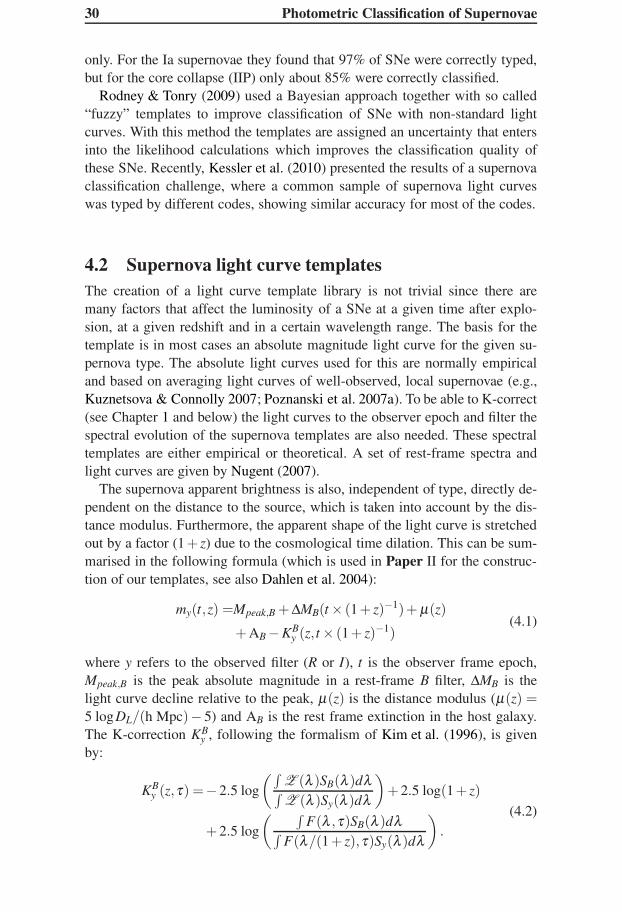
Figure 4.1: This figure shows the changes in the observed light curve of a Ia SNe asit moves to higher and higher redshift. The black line indicates the light curve for asource at z = 0.5. The colour indicates brightness (red is bright).

In this expression Z (λ ) is the spectral energy distribution of Vega; SB(λ ),Sy(λ ) the Johnson B and VIMOS R/I total filter transmission curves andF(λ ,τ) the spectral energy distribution of the supernova at rest frame epochτ .

The resulting templates with redshift evolution for the Ia and IIP subtypesis shown in Figures 4.1 and 4.2. Also, the template light curves for all thesubtypes was previously shown in Figure 2.1. In Paper II we also go throughthe sources for the light curve and spectral information that is used to constructthe templates given in these figures. Our template library consist of nine differ-ent supernova subtypes: Ia–normal, Ia–faint (a low stretch template), 91T-like,91bg-like, IIP, IIL, IIn, Ibc–bright and Ibc–normal.

4.3 Bayesian typing of supernovaeIn Paper II we presented the typing code used in SVISS. This code is basedon the Bayesian methodology described by Kuznetsova & Connolly (2007). In


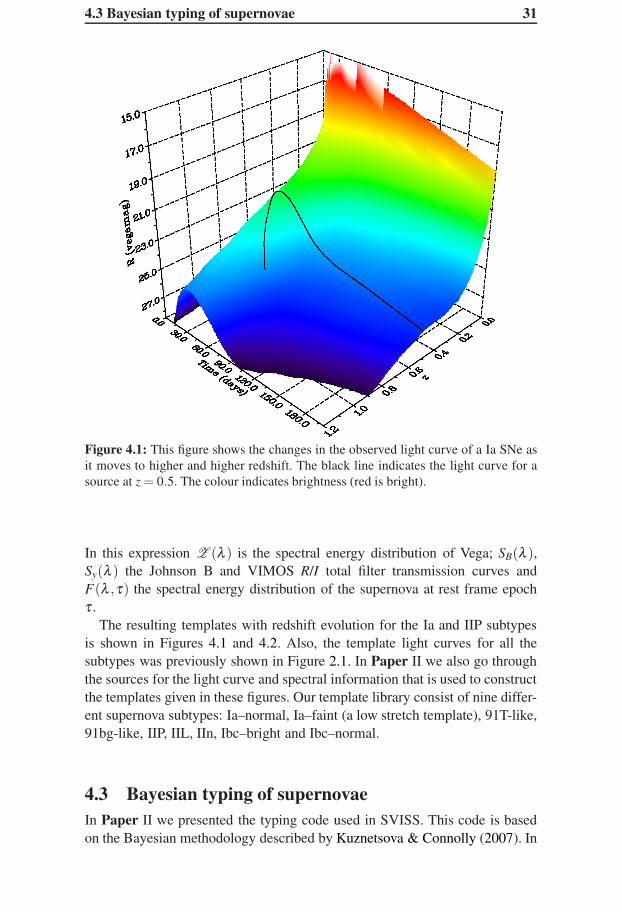
Figure 4.2: This figure shows the changes in the observed light curve of a IIP SNe asit moves to higher and higher redshift. The black line indicates the light curve for asource at z = 0.5.

χ2-fitting methods the best type is found by finding the model, for any tem-plate, that fits the data the best. This is a quite straight forward method but hassome drawbacks, the major one is that it doesn’t allow prior information on,e.g., redshifts and peak luminosity, to be used to full extent. In Bayesian typ-ing any prior information that can be expressed as a probability distribution iseasily utilised in the typing. Furthermore, by marginalising over the parameterprobability distributions it is possible to find the most likely supernova typetaking the fitting quality of all possible parameter combinations for a giventype into account, rather than just the best fitting parameter set. In other words,in Bayesian typing the entire parameter space for a given SN type is comparedto the observations and the best type selected, while normal maximum likeli-hood methods only look at the very best fit for each type. For reference, I heresummarise the details of the method.

We want to find the type that maximises the probability P(T j|Fi), i.e. themost likely type, T j, for a given light curve Fi. The index j = [1, ...,NT ]refers to the different types and i = [1, ...,Ndp] to the points on the observedlight curve. Nine supernova types (Ia, Ia f aint , 91bg-like, 91t-like, Ibcnormal ,


Ibcbright , IIn, IIL and IIP) have been considered. The total number of datapoints (Ndp) is given by the product of the number of filters (N f ilters) and thenumber of observation epochs (Nep). The probability P(T j|Fi) cannot becalculated directly, but by using Bayes’ theorem we can rewrite the probabil-ity:

P(T j|Fi) =P(Fi|T j)P(T j)

∑ j P(Fi|T j)P(T j). (4.3)

P(Fi|T j) is the probability of obtaining the light curve data Fi for a givensupernova type T j. P(T j) contain all prior information on the supernova modellight curve for the specific type. When Bayes’ theorem is used in this fashionwe implicitly assume that the set of supernova types is complete, i.e. all super-nova candidates must be one of the considered types. For sufficiently peculiarsupernovae, and non-supernovae, Equation 4.3 will not give valid probabilities.

The nine supernova subtype templates are determined by four parametersthat uniquely define the light curve for a given type: (i) MB the absolute rest-frame B band magnitude at peak, (ii) z, the redshift of the supernova, (iii)t, the time difference between the explosion date for the model and the firstobservational epoch,(iv) RV ,E(B−V ) = ~η; extinction in the host galaxy.We denote the template light curves by fi, j,

fi, j= fi, j(MB,z, t,~η). (4.4)

and since these parameters uniquely define the light curve for a specifictype we may rewrite P(Fi|T j) as P(Fi| fi, j(MB,z, t,~η)) and P(T j) asP(MB,z, t,~η ,T j).

We define the likelihood function for each supernova type:

l j(Fi|MB,z, t,~η)≡ P(Fi|T j)P(T j)

= P(Fi| fi, j(MB,z, t,~η))P(MB,z, t,~η ,T j).(4.5)

The probability that a supernova with a template light curve fi, j will have anobserved light curve, Fi, is

P(Fi| fi, j(MB,z, t,~η)) =Nd p

∏i

e−(Fi− fi, j)2/(2δF2

i )

√2πδFi

, (4.6)

where each observational data point is allowed to fluctuate according to Gaus-sian statistics (the widths of the distributions are given by the observationalerrors, δFi).

The P(MB,z, t,~η ,T j), or equivalently P(MB,z, t,~η |T j), prior contains allthe prior information on the parameters for a given template. We assume thatthe parameters are independent and can thus factorise the prior:

P(MB,z, t,~η |T j) = P(MB|T j)P(z|T j)P(t|T j)

×P(t|T j)P(~η |T j)P(T j).(4.7)


The assumed individual priors are further described in Paper II. Some of them,P(T j), P(t) and P(~η) are so called flat priors, meaning that all possible valuesfor that parameter have the same probability of occurring. The two remainingpriors, on z and MB, contain a priori information from probability distributionsfrom the host photometric redshift in the former case and observations of localSNe in the later case.

When trying to find the most likely supernova type the four parameters areall nuisance parameters; we marginalise the likelihood function over the fourparameters to get the summed likelihood function, or in Bayesian terms, theevidence:

L j = ∑MB

∑z

∑t

∑~η

P(Fi| fi, j(MB,z, t,~η))P(MB,z, t,~η ,T j). (4.8)

The probability P(T j|Fi) is then equal to the relative evidence for each su-pernova type,

P(T j|Fi) =L j

∑ j L j

. (4.9)

The most likely type for a given SN candidate is the one with the highestP(T j|Fi). We co-add the probabilities for the subtypes belonging to eitherof the two main types (thermonuclear and core collapse types) and get theprobabilities P(T N) and P(CC) for each typed supernovae.

The Bayesian method outlined above was implemented as a FORTRAN 90code. The speed of the code critically depends on the resolution and range ofthe considered priors. For the normal setup, the time it takes to type one super-nova is approximately 15 minutes (on a 1.8 GHz core). During the extensivetesting of the code we typed thousands of supernovae, which meant that thecode had to be parallelised, this was done using the LAM-MPI framework.

In Paper II we also made tests on the typing method by creating a MonteCarlo simulated sample of supernova light curves. These light curves wereconstructed from the templates used for the typing with random errors addedand propagated. It should be noted that the typing quality assessments made inthis way have to be treated with some caution, since the testing is only reallyvalid if the template light curves are representative of all observed SNe. Thisis not necessarily the case and the tests on the simulated light curves is thusmore of a test on the internal consistency of the code. Nevertheless, our testsindicated that the resulting subtype classifications within the two main types(CC and Ia) are prone to quite large errors (on the order of 10–20%), while theerrors on the main type classifications are significantly smaller (on the order of5–10%). The typing quality is also shown in Figure 4.3. The supernova subtypethat is hardest to type is clearly the Ibcnormal supernovae. We also found thatthe mistyping between Ia and CC SNe is not symmetric, more core collapseSNe are mistyped as Ia SNe than the other way around.

The typing code was also tested on a sample of real supernovae (Ia and IIP)from the Sloan Digital Sky Survey supernova search (Frieman et al. 2008).


Figure 4.3: This figure shows the resulting photometric type distribution for simulatedlight curves of types: (a) 91bg-like, (b) 91T-like, (c) Ia–faint, (d) Ia, (e) Ibc–bright, (f)Ibc–normal, (g) IIL, (h) IIn, (i) IIP. The accuracy of the subtype classifications issignificantly worse than the accuracy for a simple core collapse–Ia division.

These tests are also reported in Paper II, the percentage of mistyped super-novae for this sample was 5–10%. Since this value is quite similar to the onefound in the extensive Monte Carlo simulations, we concluded that these testsare representative of the true typing accuracy. Of course, tests on a larger sam-ple of real, high redshift SNe (such as the sample used in Kessler et al. 2010),could provide a safer estimate of the accuracy.

The 16 supernovae discovered in the SVISS were typed using our code. Wefound that eight of them were most likely to be core collapse SNe and that theother eight were most likely to be Ia SNe. In Figure 3.7 I show an exampleof a SN light curve with the best fitting model light curve. The typing methodapplied to the SVISS supernovae is further discussed in Paper II.

37

5 Supernova Rates

Supernova rates have traditionally been very hard to estimate due to the rarityof the supernovae themselves. At high redshift it becomes even harder becauseof their apparent faintness. It is only in the latest decades, with major devel-opments in both telescope and instrument technology that it has been possibleto cover large enough volumes for imaging surveys to detect more than a fewSNe. Figures 5.1 and 5.2 (from Paper IV, reprinted here for easy reference)show a compilation of rates from the major supernova surveys together withthe results from the SVISS.

5.1 Earlier work on supernova ratesMuch of the work that has been done on Ia rates comes from the large Ia sur-veys designed to find spectroscopically confirmed SNe to use for precisioncosmology (e.g., Perlmutter et al. 1997; Riess et al. 1998; Astier et al. 2006;Riess et al. 2007). At low redshift, the recently reported rates from the LOSS(Li et al. 2011a) are the most accurate determination of the rates so far. Ear-lier work by Cappellaro et al. (1999) show a similar rate. At slightly higherredshifts, z ∼ 0.3, Ia rates have been measured by STRESS (Botticella et al.2008) and SDSSII (Dilday et al. 2010). The Ia rates from SNLS (Neill et al.2006) at z ∼ 0.5 are based on a large number of SNe and is likely the most se-cure data point at this redshift range. Rodney & Tonry (2010) present revisedIa rates from the IfA Deep Survey, lower than those previously reported, outto z = 1.05 using new techniques. At even higher redshifts few rate measure-ments are available, the GOODS supernova search reports rates out to z ∼ 1.7(Dahlen et al. 2008). Graur et al. (2011) recently reported the Ia rates fromthe Subaru Deep Field supernova search which reach similar redshifts as theGOODS results. Both of these surveys show a remarkably low rate of Ia su-pernovae at high redshift, a point I will come back to later in this chapter.

For core collapse SNe, fewer rate measurements have been reported. Thisis partly because they are harder to find, being intrinsically fainter than Ia andmore subjected to host galaxy extinction, but also that they are not interestingfor the surveys with mainly cosmological goals. At low redshift the rates deter-mined by the LOSS (Li et al. 2011a) provide an accurate rate estimate, whichis very similar to the CC rate measurement of Cappellaro et al. (1999). Goingto higher redshift (z ∼ 0.3) CC rates have been measured by Cappellaro et al.(2005) and STRESS (Botticella et al. 2008) and SNLS (Bazin et al. 2009). The

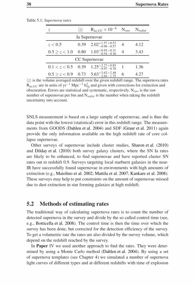
38 Supernova Rates

Table 5.1: Supernova rates

z 〈z〉 RIa/CC ×10−4 Nraw Nredist

Ia Supernovae

z < 0.5 0.39 2.02+1.57+0.53−0.96−0.57 4 4.12

0.5 ≥ z < 1.0 0.80 1.03+0.92+0.31−0.54−0.36 4 3.43

CC Supernovae

0.1 < z < 0.5 0.39 1.25+2.27+0.85−0.97−0.78 1 1.36

0.5 ≥ z < 0.9 0.73 5.63+3.62+2.48−2.64−1.75 6 4.27

〈z〉 is the volume averaged redshift over the given redshift range. The supernova ratesRIa/CC are in units of yr−1 Mpc−3 h3

70 and given with corrections for extinction andobscuration. Errors are statistical and systematic, respectively. Nraw is the rawnumber of supernovae per bin and Nredist is the number when taking the redshiftuncertainty into account.

SNLS measurement is based on a large sample of supernovae, and is thus thedata point with the lowest (statistical) error in this redshift range. The measure-ments from GOODS (Dahlen et al. 2004) and SDF (Graur et al. 2011) againprovide the only information available on the high redshift rate of core col-lapse supernovae.

Other surveys of supernovae include cluster studies, Sharon et al. (2010)and Dilday et al. (2010) both survey galaxy clusters, where the SN Ia ratesare likely to be enhanced, to find supernovae and have reported cluster SNrates out to redshift 0.9. Surveys targeting local starburst galaxies in the near-IR have successfully found supernovae in environments with high amounts ofextinction (e.g., Maiolino et al. 2002; Mattila et al. 2007; Kankare et al. 2008).These surveys may help to put constraints on the amount of supernovae misseddue to dust extinction in star forming galaxies at high redshift.

5.2 Methods of estimating ratesThe traditional way of calculating supernova rates is to count the number ofdetected supernova in the survey and divide by the so called control time (see,e.g., Botticella et al. 2008). The control time is then the time over which thesurvey has been done, but corrected for the detection efficiency of the survey.To get a volumetric rate the rates are also divided by the survey volume, whichdepend on the redshift reached by the survey.

In Paper IV we used another approach to find the rates. They were deter-mined by using a Monte Carlo method (Dahlen et al. 2004). By using a setof supernova templates (see Chapter 4) we simulated a number of supernovalight curves of different types and at different redshifts with time of explosion

5.3 Comparing supernova rates to the star formation history 39

set as to be detectable in our observational window. Each supernova was alsogiven a host galaxy extinction based on the work of Hatano et al. (1998) andRiello & Patat (2005).

The light curves then went through the same detection procedure as the realsupernova light curves. We have also used the detection efficiencies derivedfrom the simulation described in Paper I. The output rates from the simula-tions are then compared to the observed rates in the chosen redshift bins. Thesimulations are rerun until the output rates match the observed ones. At thatpoint the input intrinsic SN rate is chosen as the true supernova rate. The foundrates with statistical errors estimated using Gehrels (1986) and systematic er-rors (see Section 5.5) are given in Table 5.1 (and, of course, in Paper IV).

5.3 Comparing supernova rates to the star formationhistoryThe core collapse supernova rate can be compared to the cosmic star forma-tion history (SFH), since the timescale for CC progenitors to explode is muchshorter than the cosmic timescale, the CC rate traces the instantaneous cosmicSFR. The supernova rate is derived from the star formation history by assum-ing an Initial Mass Function (IMF, denoted by ξ below) and the mass rangeof the SN progenitors (Ml and Mu for the lower and upper mass limits, re-spectively). The volumetric rate of CC SNe, RCC in units of yr−1 Mpc−3 isthen:

RCC(z) = k×ρ∗(z), (5.1)

where ρ∗(z) is the star formation history in units of M⊙ yr−1 Mpc−3. RCC

is a volumetric rate, and thus scales as h3, this needs to be addressed whencomparing to star formation histories which may have a different scaling. Theconstant k is the percentage of stars that explode as SNe per unit mass and isgiven by:

k =

∫Mu

Mlξ (M)dM

∫ 125M⊙0.1M⊙ Mξ (M)dM

. (5.2)

For the SFH conversions used in Paper IV and shown in Figure 5.2 we chooseto use a Salpeter IMF (Salpeter 1955) with progenitor masses between M⊙and M⊙. The constant k is then equal to 0.0069.

The upper limit for the progenitor mass comes from Tsujimoto et al. (1997)and is essentially the limit at which massive stars will become black holesinstead of neutron stars with an associated supernova explosion. The lowerlimit of 8M⊙ is based on observations of supernova progenitors (Smartt et al.2009). The effect of changing the IMF and the mass limits for the comparisonis discussed in Paper IV.

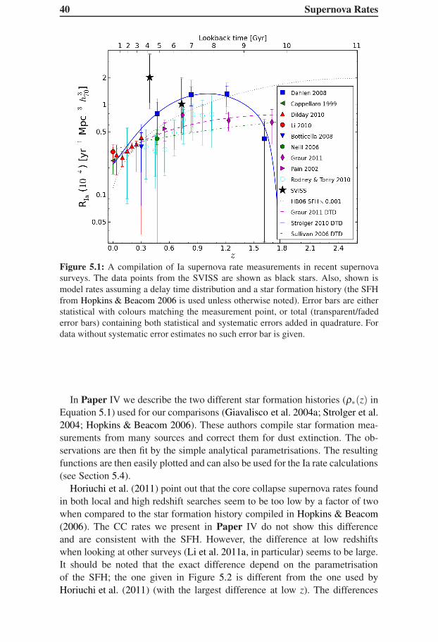
40 Supernova Rates

Figure 5.1: A compilation of Ia supernova rate measurements in recent supernovasurveys. The data points from the SVISS are shown as black stars. Also, shown ismodel rates assuming a delay time distribution and a star formation history (the SFHfrom Hopkins & Beacom 2006 is used unless otherwise noted). Error bars are eitherstatistical with colours matching the measurement point, or total (transparent/fadederror bars) containing both statistical and systematic errors added in quadrature. Fordata without systematic error estimates no such error bar is given.

In Paper IV we describe the two different star formation histories (ρ∗(z) inEquation 5.1) used for our comparisons (Giavalisco et al. 2004a; Strolger et al.2004; Hopkins & Beacom 2006). These authors compile star formation mea-surements from many sources and correct them for dust extinction. The ob-servations are then fit by the simple analytical parametrisations. The resultingfunctions are then easily plotted and can also be used for the Ia rate calculations(see Section 5.4).

Horiuchi et al. (2011) point out that the core collapse supernova rates foundin both local and high redshift searches seem to be too low by a factor of twowhen compared to the star formation history compiled in Hopkins & Beacom(2006). The CC rates we present in Paper IV do not show this differenceand are consistent with the SFH. However, the difference at low redshiftswhen looking at other surveys (Li et al. 2011a, in particular) seems to be large.It should be noted that the exact difference depend on the parametrisationof the SFH; the one given in Figure 5.2 is different from the one used byHoriuchi et al. (2011) (with the largest difference at low z). The differences

5.4 Constraining the Ia delay time distribution 41

could also possibly be explained by a larger amount of SNe being missed dueto host galaxy extinction (see Section 5.6).

5.4 Constraining the Ia delay time distributionThe delay time distribution (DTD) for Ia supernovae is an interesting subjectand is the subject of controversy in current research. By convolving an assumedDTD with the underlying star formation history the Ia rate can be calculated.This can then be compared with the observed rates to put constraints on theDTDs. The Ia rate can thus be written (Strolger et al. 2004):

RIa(t) = ν

∫ t

t0

ρ∗(t′)Φ(t − t ′)dt ′, (5.3)

where ν is the number of SNe formed per unit stellar mass, ρ∗(t) the starformation history and Φ(τ) the delay time distribution which represents thepercentage of supernovae that go off at time τ after a single burst of star for-mation. Also, t0 is the time at which stars start to form in the universe, weassume this happens at z = 10; corresponding to a time of 0.45 Gyrs after theBig Bang (with our chosen cosmology). The integral can easily be convertedto redshift space to yield RIa(z) by performing a variable substitution.

In Paper IV we present the different DTDs and star formation histories thatare used to compute the model Ia rates used for comparison. The simplestone is just a rescaling of the star formation history assuming that one Ia SNeexplode per 1000M⊙ of stellar mass formed (Neill et al. 2006). This corre-sponds to using a Dirac delta function DTD with the peak at τ = 0, i.e., nodelay time between the SN explosion and star formation or, in other words, aprompt channel for the Ia progenitor-to-supernova process.

The GOODS Ia rates have been shown to be best fit by Gaussian shaped (orclose to Gaussian) DTD with a mean delay time of ∼ 3 Gyrs (Strolger et al.2004, 2010). These kind of DTDs can be explained for SD progenitor mod-els, but are harder to reconcile with DD models (Yungelson & Livio 2000;Strolger et al. 2004). The main difference in the resulting rates for these mod-els is the sharp decrease of Ia rates at z & 1. These models thus disfavoura prompt channel for Ia supernovae where the supernova rates would be ex-pected to follow (at least to some degree) the star formation history.

Graur et al. (2011) fit the results from the SDF supernova search togetherwith the rates of many other surveys using different power law DTDs and com-pare to other models. They find that the power law DTDs seem to be preferred,these distributions are common for DD models (e.g. Maoz et al. 2010).

Scannapieco & Bildsten (2005), Mannucci et al. (2006) and Sullivan et al.(2006b) find strong evidence for the existence of a prompt channel for Ia SNeby looking at the properties of the host galaxies of Ia SNe (and other data).Maoz et al. (2011) study the hosts of the local SNe found in the LOSS and

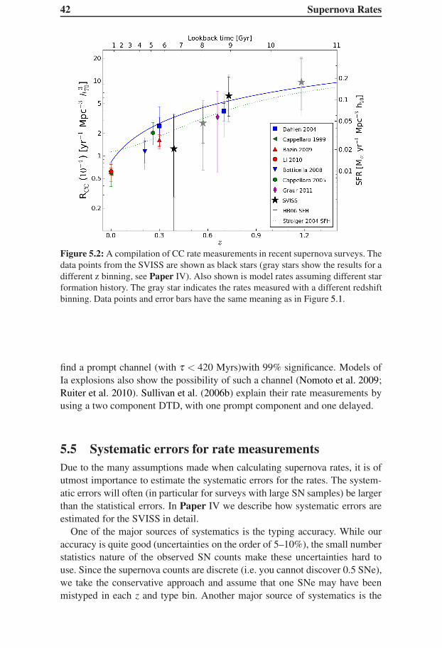
42 Supernova Rates

Figure 5.2: A compilation of CC rate measurements in recent supernova surveys. Thedata points from the SVISS are shown as black stars (gray stars show the results for adifferent z binning, see Paper IV). Also shown is model rates assuming different starformation history. The gray star indicates the rates measured with a different redshiftbinning. Data points and error bars have the same meaning as in Figure 5.1.

find a prompt channel (with τ < 420 Myrs)with 99% significance. Models ofIa explosions also show the possibility of such a channel (Nomoto et al. 2009;Ruiter et al. 2010). Sullivan et al. (2006b) explain their rate measurements byusing a two component DTD, with one prompt component and one delayed.

5.5 Systematic errors for rate measurementsDue to the many assumptions made when calculating supernova rates, it is ofutmost importance to estimate the systematic errors for the rates. The system-atic errors will often (in particular for surveys with large SN samples) be largerthan the statistical errors. In Paper IV we describe how systematic errors areestimated for the SVISS in detail.

One of the major sources of systematics is the typing accuracy. While ouraccuracy is quite good (uncertainties on the order of 5–10%), the small numberstatistics nature of the observed SN counts make these uncertainties hard touse. Since the supernova counts are discrete (i.e. you cannot discover 0.5 SNe),we take the conservative approach and assume that one SNe may have beenmistyped in each z and type bin. Another major source of systematics is the

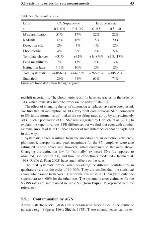
5.5 Systematic errors for rate measurements 43

Table 5.2: Systematic errors

Error CC Supernovae Ia Supernovae

z 0.1–0.5 0.5–0.9 0–0.5 0.5–1.0

Misclassification 51% 17% 22% 22%

Redshift 32% 16% 15% 20%

Detection eff. 2% 3% 1% 2%

Photometric 4% 9% 2% 5%

Template choices +31% +32% +1/-8%% +2%/-17%

Peak magnitudes 7% 15% 2% 3%

Extinction laws . 1% 10% 2% 2%

Total systematic +68/-62% +44/-31% +26/-28% +30/-35%

Statistical 129% 61% 63% 71%Errors are two-sided unless the sign is given.

redshift uncertainty. The photometric redshifts have accuracies on the order of10% which translates into rate errors on the order of 10–30%.

The effect of changing the set of supernova templates have also been tested.We find that an assumption of 30% very faint core collapse SNe (comparedto 8% in the normal setup) makes the resulting rates go up by approximately30%. Such a population of CC SNe was suggested by Horiuchi et al. (2011) toexplain the supernova rate–SFH difference, but we find that even with a ratherextreme amount of faint CC SNe a factor of two difference cannot be explainedin this way.

Systematic errors resulting from the uncertainties in detection efficiency,photometric zeropoints and peak magnitude for the SN templates were alsoestimated. These errors are, however, small compared to the ones above.Changing the extinction law for “normally” extincted SNe (as opposed toobscured, see Section 5.6) and how the extinction i modelled (Hatano et al.1998; Riello & Patat 2005) have small effects on the rates.

The total systematic errors (when co-adding the different contributions inquadrature) are on the order of 30-60%. They are smaller than the statisticalerrors which range from over 100% for the low redshift CC bin (with only onesupernova) to ∼ 60% for the other bins. The systematic error estimates for theSVISS rates are summarised in Table 5.2 (from Paper IV, reprinted here forreference).

5.5.1 Contamination by AGN

Active Galactic Nuclei (AGN) are super-massive black holes in the centre ofgalaxies (e.g., Salpeter 1964; Shields 1978). These cosmic beasts can be ex-

44 Supernova Rates

tremely luminous and appear as point sources in imaging surveys. Furthermorethey are situated in the centre of their host galaxies and show optical variability(e.g., Stalin et al. 2004) . This means that they may be mistaken for supernovaein surveys without spectra and with short observation periods. Cappellaro et al.(2005) correct for this by assuming that 40% of the variable objects found inthe centre of their host galaxies are in fact AGN.

For the SVISS observations we obtained an additional observational epoch,one year after the last SN search epoch (see Paper II). This epoch is usedto reject SN candidates that show variability over a longer time period thanwhat is possible for SNe. The difference in variabilities between SNe andAGN have been used to reject SNe in searches for AGN (Boutsia et al. 2009;Villforth et al. 2010).

5.6 The effect of host galaxy extinction on the ratesSupernovae exploding in spiral galaxies (and to much lesser extent, ellipticalgalaxies) are subject to extinction from dust and gas in the host galaxy. Thiseffect was observationally confirmed when it was discovered that fewer SNewere found in inclined spiral galaxies (e.g. van den Bergh & Tammann 1991),where the light from the supernovae has to pass through more gas and dust thanin a non-inclined galaxy. Hatano et al. (1998) and Riello & Patat (2005) madesimulations to determine the average extinction for SNe using galaxy modelsand Monte Carlo simulations for CC and Ia supernovae, respectively.

Using these estimates of SN extinction is only valid if we assume that theSNe explode in the type of galaxies used in the simulations. But as we go tohigher redshifts the bulk of star formation is no longer taking place in these“normal” galaxies but rather in galaxies with high amounts of dust (in theso called Luminous and Ultra-Luminous Infrared Galaxies, LIRGs/ULIRGs).Le Floc’h et al. (2005) find that approximately 70 % of the star formation atz ∼ 1 is taking place in LIRGs, and present how this fraction changes withredshift from low to high redshift. These galaxies have a much higher contentof dust and most SNe in them will suffer from high amounts of extinction.Searches for SNe in similar systems at low z, has shown that optical searchesmiss almost all SNe that explode in them (e.g. Mattila et al. 2004). In Paper IVwe denote this effect obscuration.

Mannucci et al. (2007) use the results of Le Floc’h et al. (2005) togetherwith an estimate on how many SNe that are lost to obscuration by dust inlocal galaxies to derive a correction for core collapse supernova rates at highredshifts. This correction is given by the function:

fCC(z) = 0.05+0.28z, (5.4)

valid for z ≤ 2 and where fCC is the fraction of CC SNe missed at redshift z.

5.6 The effect of host galaxy extinction on the rates 45

Ia SNe are not as strongly coupled to star formation as core collapse SNe.Assuming that some of Ia SNe originate from the prompt channel (see Sec-tion 5.4), which is coupled to the star formation, Mannucci et al. (2007) find acorrection factor of:

fIa = 0.02+0.12z1.4, (5.5)

valid for z ≤ 2 for the Ia rates. It should be noted that this correction is moreuncertain than the one for CC given in Equation 5.4, given that it dependscritically on the assumed DTD for Ia SNe.

We apply these correction to the SVISS rates reported in Paper IV, but alsogive un-corrected values. The assumptions on extinction and obscuration in thehost galaxies will of course also introduce systematic errors. The obscurationcorrections for higher redshifts given by Mannucci et al. (2007) do not haveany associated uncertainties and are thus not included in the systematic errorestimates above. The effects of using different extinction models for normalgalaxies (Hatano et al. 1998; Riello & Patat 2005) have also been studied andresults in small uncertainties.

47

6 Summary of the papers

The focus of my thesis is the classification of supernovae and the calculationof supernova rates using survey data. In this chapter I give a summary of thepapers that are included in this thesis, and describe my contributions to each ofthem. For all of the papers it should be noted that the authors listed on the au-thor list all contributed to the papers in the form of very important discussionson how to interpret and analyse the survey data.

In Paper I we explored how to detect supernovae optimally with particu-lar focus on the image subtraction method. We performed detailed tests bysimulating supernovae in the images and then tried to recover them with cor-rect photometry. The main result from this paper was how to tweak the imagesubtraction code to produce optimal results. Another important result was thediscovery that the normal way of estimating photometric errors failed in sub-tracted images, and that we found out how to do it instead. The work done inthis paper was also very important for Papers II and IV. I wrote this paper anddid all of the work on simulations and image subtraction in it. I had help withdoing the reductions for the data used and also on the tweaking of the imagesubtraction code.

In Paper II we presented a list of 16 supernovae found in the SVISS. Wealso introduced a photometric method of typing supernovae into the core col-lapse or Ia type. This typing code was tested on a simulated set of SN lightcurves and on a sample of real light curves with know type. The method ofdetecting the SNe and making sure that they actually were SNe was also de-scribed. My contribution to this paper was the detection of the SNe and doingthe measurements for the light curves. I also wrote the typing code and per-formed the testing on it. I wrote this paper, except for the part on the MonteCarlo simulated supernova light curves. I had help with computing the photo-metric redshifts and with the creation of the Monte Carlo simulated supernovalight curves used for the code testing. The manual rejection step of the super-nova rejection scheme was a collaborative effort of the entire team.

The reduction pipeline and photometric galaxy catalogues were presentedin Paper III. The purpose of this paper was mainly to release our galaxy cat-alogues and describe how they were constructed. The novel stacking methodsinvolving optimal weighting schemes were described. We also computed num-ber counts and photometric redshifts for the galaxy catalogue. We used evo-lutionary tracks for different types of galaxies to make Lyman Break Galaxyselection criteria and showed number counts for these galaxies. The U band

48 Summary of the papers

counts for our LBGs were found to be among the deepest ever observed. Mycontribution to this paper was to the work on the image reduction pipeline, Ialso helped with reducing the data set. I was also part of problem searchingand discussions relating to the observations. I did not do any writing for thispaper.

Finally, in Paper IV we reported the supernova rates calculated from theSVISS. The rates were computed using a Monte Carlo-based method. We alsoinvestigated the systematic errors that may have an effect on the rates in greatdetail. We discussed the implications of our rate measurements on the cosmicstar formation history and the Ia delay time distribution. I wrote this paper andcompiled the comparisons to other surveys, to the star formation histories forCC SNe, and to delay time distributions for the Ia SNe. I also computed the de-tection efficiencies used in the rate calculations and investigated the systematicerrors. I had help with computing the rates using the Monte Carlo simulations.

49

7 Svensk sammanfattning avavhandlingen

Frekvensen av supernovor i det tidiga universum

Supernovor är kosmiska explosioner av kolossal omfattning som markerar enstjärnas död. Utöver att vara intressanta fenomen att studera för sig så gör derasljusstyrka dem till utmärkta mätinstrument för att studera det tidiga universum.Beroende på vilken typ av stjärna som exploderat och hur detta gick till så kanolika fysikaliska processer studeras.

I den här avhandlingen presenteras det arbete jag har gjort med upptäckan-det, analyserandet och frekvensmätningar av supernovor i “Stockholm VIMOSSupernova Search”. Vi upptäckte 16 supernovor som exploderade för flera mil-jarder år sedan (eller med andra ord, med höga rödförskjutningar). Den upp-mätta variationen av ljusstyrka och färg för supernovorna har använts för attklassificera dem som antingen termonukleära (typ Ia) supernovor, eller somkärnkollapssupernovor (typ II). Noggrannheten hos vår klassifikationskod ärgod, endast ungefär 5% av supernovorna blir felklassificerade, vilket är mot-svarande den noggrannhet som andra koder av denna typ har uppnått.

Genom att jämföra den observerade frekvensen av supernovorna med simu-leringar så kan den bakomliggande supernovafrekensen vid höga rödförskjut-ningar mätas upp. Huvudresultatet i denna avhandling är att frekvensen avkärnkollapssupernovor vid höga rödförskjutningar matchar det man kan för-vänta sig från att titta på den generella stjärnbildningshastigheten i universum,och att de matchar tidigare studier som gjorts. Frekvensen av Ia-supernovorvid höga rödförskjutningar har uppmätts av ett flertal andra projekt, våra resul-tat visar på en något högre frekvens än förväntat. Vi undersökte även de olikasystematiska fel som kan påverka frekvensmätningarna.

Dessutom har vi, genom använda oss av nyskapande metoder för att behand-la och lägga ihop astronomiska bilder, skapat en katalog som innehåller nära50.000 galaxer i vårt observationsfält. Fotometrisk rödförskjutning har beräk-nats för de flesta av galaxerna med en noggrannhet som är i storleksordningen10%. Galaxkatalogen har även använts för hitta galaxer med höga rödförskjut-ningar, så kallade “Lyman Break-galaxer”.

51

Publications not included in this thesis

I Supernovae 2003gk and 2003glSollerman J., Andersson J., [4 authors], IAU circular, 8164, 3(my surname was Andersson before june 2004)

II GRB 050509B: Constraints on Short Gamma-Ray BurstModelsHjorth J., [5 authors], Melinder J., [15 authors], ApJ, 630, L117

III SN 2003du: 480 days in the life of a normal type Ia supernovaStanishev V., [24 authors], Melinder J., [6 authors] ,2007, A&A,469, 645S

IV Escape of about five per cent of Lyman-α photons from high-redshift star-forming galaxiesHayes M., [8 authors], Melinder J., 2010, Nature, 464, 562

53

Acknowledgements

During my time as a PhD student I have worked together with many people.I have also had a lot of fun together with people I’ve met during my PhD, aswell as with other, older acquaintancies. Here I would like to acknowledgethose people.

I’d like to acknowledge the help and support of Claes Fransson, my thesissupervisor. His impressive breadth of knowledge in astronomy, physics andsupernovae in particular has been very helpful over the years. Thank you forteaching me how to do research and how to present it. I’m also grateful foradditional financial support without which this thesis would never have beenwritten.

Thank you Göran Östlin for being a great departmental boss and for thehelp over the years on all things observational and for your valuable contribu-tion to the SVISS project. I have learnt a lot from the discussions and brain-storming sessions we’ve had. Thank you Laia Mencía Trinchant for beinga great co-worker, friend and officemate. Without you, the project would stillhave been stuck on photometric calibrations. Thanks Seppo Mattila for help-ing me get started with the supernova detections and for being a driving forcein the project. I’m also very grateful for the financial support you managed tosecure for me. Thank you Tomas Dahlen for helping me out with the super-nova typing and rates and for all of the other stuff you’ve done for the project.Also, thanks for making me feel welcome during my short stay in Baltimore.Thank you Jesper Sollerman for good advice on the observational aspects ofsupernovae and for the help with many different things you’ve given me overthe years.

I’d like to thank the members of my thesis group, Claes-Ingvar Björnssonand Göran Olofsson. Thanks for checking on me from time to time and forbelieving in my abilities even when I doubted myself.

Thank you Matt for being a great friend and for the really nice discus-sions on everything from the latest astro-ph papers to the proper way to correctimages for birds. Thanks for convincing me that the temperature is alwaysfine (in the office that is). Thank you Jacob for your friendship, for being agreat listener and for all the great pub visits. It was a fun year sitting in theboard together with you, trying to get changes through (stuff which is moreor less all implemented by now). Thank you Sofia for being a good friendand officemate and for showing that it is possible to have children and beinga productive scientist at the same time. I’d also like to thank present and past

54 Acknowledgements

PhD students that I have studied, worked, had weird lunch conversations with,partied with, etc. Thank you Anestis, Angela, Anders, Gautam, Genoveva,Michael, Matthias, Theresa, Javier, Nuria, Ricky, Jaime, Vasco, Natalia,Thomas M., Tanja, Per, Zita, Soroush and Andreas A. L..

I’d also like to thank some other people at the department. Thank you Ullafor your help with many administrative issues durung the first years of my PhD.I really enjoyed working together with you on the student course registrations.Thank you Sandra for your help with forms even when I’ve been late. Also,thanks for organizing all the social gettogethers at the department, it meansa lot to all of us. Thanks Lena for your help with salary related stuff andfor always being friendly and interested in what people have to say. Thankyou Sergio for all the computer help I’ve received over the years, thanks foranswering some really stupid questions. Thank you Cecilia for welcoming meto the department and for all the good advice during the first couple of yearsof my PhD.

I’d like to mention some of my other friends that have helped me escapefrom reality and allowed me to forget all about astronomy from time to time.Thank you Claes and David for the fun we’ve had and will have in the future.Thank you Henrik, Niclas and Peter for some really fun weekends.

When I was growing up and starting to become interested in astronomy Ialways had the support from my parents. Thank you Mamma and Pappa foralways believing in me and giving me support and help when I needed it themost. Thank you, rest of my family, for being interested and always wantingto hear about my research.

Thank you Love and Lilly for bringing so much joy into my life. Finally,I’d like to thank Moa for allowing me to pursue my dream. Thank you, mylove, for everything.

55

Bibliography

Abazajian, K. N., Adelman-McCarthy, J. K., Agüeros, M. A., et al. 2009,ApJS, 182, 543

Alard, C. 2000, A&AS, 144, 363, (A00)

Alard, C. 2001, MNRAS, 320, 341

Alard, C. & Lupton, R. H. 1998, ApJ, 503, 325

Alcalá, J. M., Pannella, M., Puddu, E., et al. 2004, A&A, 428, 339

Amanullah, R., Lidman, C., Rubin, D., et al. 2010, ApJ, 716, 712

Arnett, W. D., Bahcall, J. N., Kirshner, R. P., & Woosley, S. E. 1989,ARA&A, 27, 629

Astier, P., Guy, J., Regnault, N., et al. 2006, A&A, 447, 31

Bazin, G., Palanque-Delabrouille, N., Rich, J., et al. 2009, A&A, 499, 653

Beckwith, S. V. W., Stiavelli, M., Koekemoer, A. M., et al. 2006, AJ, 132,1729

Benítez, N. 2000, ApJ, 536, 571

Berta, S., Rubele, S., Franceschini, A., et al. 2008, A&A, 488, 533

Bertin, E. & Arnouts, S. 1996, A&AS, 117, 393

Bethe, H. A. & Wilson, J. R. 1985, ApJ, 295, 14

Blinnikov, S. I. & Bartunov, O. S. 1993, A&A, 273, 106

Bolzonella, M., Miralles, J., & Pelló, R. 2000, A&A, 363, 476

Botticella, M. T., Riello, M., Cappellaro, E., et al. 2008, A&A, 479, 49

Boutsia, K., Leibundgut, B., Trevese, D., & Vagnetti, F. 2009, A&A, 497, 81

Bouwens, R. J., Illingworth, G. D., Franx, M., et al. 2009, ApJ, 705, 936

Bunker, A. J., Wilkins, S., Ellis, R. S., et al. 2010, MNRAS, 409, 855

Capak, P., Cowie, L. L., Hu, E. M., et al. 2004, AJ, 127, 180

56 BIBLIOGRAPHY

Cappellaro, E., Evans, R., & Turatto, M. 1999, A&A, 351, 459

Cappellaro, E., Riello, M., Altavilla, G., et al. 2005, A&A, 430, 83

Chandrasekhar, S. 1934, The Observatory, 57, 373

Colgate, S. A. & White, R. H. 1966, ApJ, 143, 626

Colless, M., Dalton, G., Maddox, S., et al. 2001, MNRAS, 328, 1039

Collister, A. A. & Lahav, O. 2004, PASP, 116, 345

Corwin, T. M., Sumerel, A. N., Pritzl, B. J., et al. 2006, AJ, 132, 1014

Crowther, P. A. 2007, ARA&A, 45, 177

Dahlén, T. & Goobar, A. 2002, PASP, 114, 284

Dahlen, T., Mobasher, B., Dickinson, M., et al. 2010, ApJ, 724, 425

Dahlen, T., Strolger, L.-G., & Riess, A. G. 2008, ApJ, 681, 462

Dahlen, T., Strolger, L.-G., Riess, A. G., et al. 2004, ApJ, 613, 189

Dilday, B., Smith, M., Bassett, B., et al. 2010, ApJ, 713, 1026

Feldmann, R., Carollo, C. M., Porciani, C., et al. 2006, MNRAS, 372, 565

Filippenko, A. V. 1997, ARA&A, 35, 309

Filippenko, A. V., Richmond, M. W., Branch, D., et al. 1992a, AJ, 104, 1543

Filippenko, A. V., Richmond, M. W., Matheson, T., et al. 1992b, ApJ, 384,L15

Fransson, C., Chevalier, R. A., Filippenko, A. V., et al. 2002, ApJ, 572, 350

Frieman, J. A., Bassett, B., Becker, A., et al. 2008, AJ, 135, 338

Furusawa, H., Kosugi, G., Akiyama, M., et al. 2008, ApJS, 176, 1

Gaskell, C. M., Cappellaro, E., Dinerstein, H. L., et al. 1986, ApJ, 306, L77

Gehrels, N. 1986, ApJ, 303, 336

Gerdes, D. W., Sypniewski, A. J., McKay, T. A., et al. 2010, ApJ, 715, 823

Giacconi, R., Rosati, P., Tozzi, P., et al. 2001, ApJ, 551, 624

Giavalisco, M. 2002, ARA&A, 40, 579

Giavalisco, M., Dickinson, M., Ferguson, H. C., et al. 2004a, ApJ, 600, L103

BIBLIOGRAPHY 57

Giavalisco, M., Ferguson, H. C., Koekemoer, A. M., et al. 2004b, ApJ, 600,L93

Gössl, C. A. & Riffeser, A. 2002, A&A, 381, 1095

Graur, O., Poznanski, D., Maoz, D., et al. 2011, ArXiv e-prints

Hatano, K., Branch, D., & Deaton, J. 1998, ApJ, 502, 177

Hildebrandt, H., Wolf, C., & Benítez, N. 2008, A&A, 480, 703

Hoflich, P., Khokhlov, A. M., & Wheeler, J. C. 1995, ApJ, 444, 831

Holman, M. J., Winn, J. N., Fuentes, C. I., et al. 2007, ApJ, 655, 1103

Holwerda, B. W. 2005, ArXiv Astrophysics e-prints

Hopkins, A. M. & Beacom, J. F. 2006, ApJ, 651, 142

Horiuchi, S., Beacom, J. F., Kochanek, C. S., et al. 2011, ArXiv e-prints

Israel, H., Hessman, F. V., & Schuh, S. 2007, Astronomische Nachrichten,328, 16

Janka, H., Langanke, K., Marek, A., Martínez-Pinedo, G., & Müller, B.2007, Phys. Rep., 442, 38

Jarrett, T. H., Chester, T., Cutri, R., et al. 2000, AJ, 119, 2498

Johnson, B. D. & Crotts, A. P. S. 2006, AJ, 132, 756

Kankare, E., Mattila, S., Ryder, S., et al. 2008, ApJ, 689, L97

Kashikawa, N., Shimasaku, K., Yasuda, N., et al. 2004, PASJ, 56, 1011

Kessler, R., Bassett, B., Belov, P., et al. 2010, PASP, 122, 1415

Khokhlov, A., Mueller, E., & Hoeflich, P. 1993, A&A, 270, 223

Kim, A., Goobar, A., & Perlmutter, S. 1996, PASP, 108, 190

Koekemoer, A. M., Aussel, H., Calzetti, D., et al. 2007, ApJS, 172, 196

Kron, R. G. 1980, ApJS, 43, 305

Kunz, M., Bassett, B. A., & Hlozek, R. A. 2007, Phys. Rev. D, 75, 103508

Kuznetsova, N. V. & Connolly, B. M. 2007, ApJ, 659, 530

La Franca, F., Gruppioni, C., Matute, I., et al. 2004, AJ, 127, 3075

Le Floc’h, E., Papovich, C., Dole, H., et al. 2005, ApJ, 632, 169

58 BIBLIOGRAPHY

LeFevre, O., Saisse, M., Mancini, D., et al. 2003, in Presented at the Societyof Photo-Optical Instrumentation Engineers (SPIE) Conference, Vol. 4841,Instrument Design and Performance for Optical/Infrared Ground-based Tele-scopes. Edited by Iye, Masanori; Moorwood, Alan F. M. Proceedings of theSPIE, Volume 4841, pp. 1670-1681 (2003)., ed. M. Iye & A. F. M. Moor-wood, 1670–1681

Leibundgut, B. 2000, A&A Rev., 10, 179

Leibundgut, B. & Suntzeff, N. B. 2003, in Lecture Notes in Physics,Berlin Springer Verlag, Vol. 598, Supernovae and Gamma-Ray Bursters, ed.K. Weiler, 77–90

Li, W., Chornock, R., Leaman, J., et al. 2011a, MNRAS, 317

Li, W., Leaman, J., Chornock, R., et al. 2011b, MNRAS, 413

Loh, E. D. & Spillar, E. J. 1986, ApJ, 303, 154

Longair, M. 1998, Galaxy formation (Springer Verlag)

Maeder, A. & Meynet, G. 2010, New A Rev., 54, 32

Maiolino, R., Vanzi, L., Mannucci, F., et al. 2002, A&A, 389, 84

Mannucci, F., Della Valle, M., & Panagia, N. 2006, MNRAS, 370, 773

Mannucci, F., Della Valle, M., & Panagia, N. 2007, MNRAS, 377, 1229

Maoz, D., Mannucci, F., Li, W., et al. 2011, MNRAS, 307

Maoz, D., Sharon, K., & Gal-Yam, A. 2010, ApJ, 722, 1879

Mattila, S., Meikle, W. P. S., & Greimel, R. 2004, New Astronomy Review,48, 595

Mattila, S., Väisänen, P., Farrah, D., et al. 2007, ApJ, 659, L9

McCracken, H. J., Radovich, M., Bertin, E., et al. 2003, A&A, 410, 17

Meikle, W. P. S., Mattila, S., Gerardy, C. L., et al. 2006, ApJ, 649, 332

Metcalfe, N., Shanks, T., Campos, A., McCracken, H. J., & Fong, R. 2001,MNRAS, 323, 795

Minkowski, R. 1941, PASP, 53, 224

Morokuma, T., Doi, M., Yasuda, N., et al. 2008, ApJ, 676, 163

Neill, J. D., Sullivan, M., Balam, D., et al. 2006, AJ, 132, 1126

BIBLIOGRAPHY 59

Nomoto, K. 1982, ApJ, 257, 780

Nomoto, K. 1984, ApJ, 277, 791

Nomoto, K., Kamiya, Y., Nakasato, N., Hachisu, I., & Kato, M. 2009, inAmerican Institute of Physics Conference Series, Vol. 1111, American In-stitute of Physics Conference Series, ed. G. Giobbi, A. Tornambe, G. Rai-mondo, M. Limongi, L. A. Antonelli, N. Menci, & E. Brocato, 267–276

Nomoto, K. I., Iwamoto, K., & Suzuki, T. 1995, Phys. Rep., 256, 173

Nugent, P. 2007, Peter Nugent’s Spectral Templates,http://supernova.lbl.gov/~nugent/nugent_templates.html

Pain, R., Fabbro, S., Sullivan, M., et al. 2002, ApJ, 577, 120

Peebles, P. 1993, Principles of physical cosmology (Princeton Univ Pr)

Percival, W. J., Reid, B. A., Eisenstein, D. J., et al. 2010, MNRAS, 401, 2148

Perlmutter, S., Gabi, S., Goldhaber, G., et al. 1997, ApJ, 483, 565

Phillips, M. M., Lira, P., Suntzeff, N. B., et al. 1999, AJ, 118, 1766

Popov, D. V. 1993, ApJ, 414, 712

Poznanski, D., Gal-Yam, A., Maoz, D., et al. 2002, PASP, 114, 833

Poznanski, D., Maoz, D., & Gal-Yam, A. 2007a, AJ, 134, 1285

Poznanski, D., Maoz, D., Yasuda, N., et al. 2007b, MNRAS, 382, 1169

Riello, M. & Patat, F. 2005, MNRAS, 362, 671

Riess, A. G., Filippenko, A. V., Challis, P., et al. 1998, AJ, 116, 1009

Riess, A. G., Macri, L., Casertano, S., et al. 2011, ApJ, 730, 119

Riess, A. G., Strolger, L., Casertano, S., et al. 2007, ApJ, 659, 98

Rodney, S. A. & Tonry, J. L. 2009, ApJ, 707, 1064

Rodney, S. A. & Tonry, J. L. 2010, ApJ, 723, 47

Ruiter, A. J., Belczynski, K., Sim, S. A., et al. 2010, ArXiv e-prints

Ruiz-Lapuente, P., Burkert, A., & Canal, R. 1995, ApJ, 447, L69+

Sako, M., Bassett, B., Becker, A., et al. 2008, AJ, 135, 348

Salpeter, E. E. 1955, ApJ, 121, 161

http://supernova.lbl.gov/~nugent/nugent_templates.html

60 BIBLIOGRAPHY

Salpeter, E. E. 1964, ApJ, 140, 796

Scannapieco, E. & Bildsten, L. 2005, ApJ, 629, L85

Sharon, K., Gal-Yam, A., Maoz, D., et al. 2010, ApJ, 718, 876

Shields, G. A. 1978, Nature, 272, 706

Smartt, S. J. 2009, ARA&A, 47, 63

Smartt, S. J., Eldridge, J. J., Crockett, R. M., & Maund, J. R. 2009, MNRAS,395, 1409

Sollerman, J., Cumming, R. J., & Lundqvist, P. 1998, ApJ, 493, 933

Spergel, D. N., Bean, R., Doré, O., et al. 2007, ApJS, 170, 377

Stalin, C. S., Gopal Krishna, Sagar, R., & Wiita, P. J. 2004, Journal of As-trophysics and Astronomy, 25, 1

Stark, D. P., Ellis, R. S., Bunker, A., et al. 2009, ApJ, 697, 1493

Stephenson, F. R. & Green, D. A. 2005, Journal for the History of Astron-omy, 36, 217

Sterken, C. & Manfroid, J. 1992, Astronomical photometry: a guide(Springer)

Stritzinger, M., Leibundgut, B., Walch, S., & Contardo, G. 2006, A&A, 450,241

Strolger, L., Dahlen, T., & Riess, A. G. 2010, ApJ, 713, 32

Strolger, L., Riess, A. G., Dahlen, T., et al. 2004, ApJ, 613, 200

Sullivan, M., Howell, D. A., Perrett, K., et al. 2006a, AJ, 131, 960

Sullivan, M., Le Borgne, D., Pritchet, C. J., et al. 2006b, ApJ, 648, 868

Sumi, T., Wozniak, P. R., Udalski, A., et al. 2006, ApJ, 636, 240

Tody, D. 1986, in Presented at the Society of Photo-Optical InstrumentationEngineers (SPIE) Conference, Vol. 627, Society of Photo-Optical Instrumen-tation Engineers (SPIE) Conference Series, ed. D. L. Crawford, 733–+

Totani, T., Morokuma, T., Oda, T., Doi, M., & Yasuda, N. 2008, PASJ, 60,1327

Tsujimoto, T., Yoshii, Y., Nomoto, K., et al. 1997, ApJ, 483, 228

Turatto, M. 2003, in Lecture Notes in Physics, Berlin Springer Verlag, Vol.598, Supernovae and Gamma-Ray Bursters, ed. K. Weiler, 21–36

BIBLIOGRAPHY 61

van den Bergh, S. & Tammann, G. A. 1991, ARA&A, 29, 363

Vanzella, E., Cristiani, S., Fontana, A., et al. 2004, A&A, 423, 761

Villforth, C., Koekemoer, A. M., & Grogin, N. A. 2010, ApJ, 723, 737

Wood-Vasey, W. M., Miknaitis, G., Stubbs, C. W., et al. 2007, ApJ, 666, 694

Woosley, S. & Janka, T. 2005, Nature Physics, 1, 147

Woosley, S. E., Heger, A., & Weaver, T. A. 2002, Reviews of ModernPhysics, 74, 1015

Yungelson, L. R. & Livio, M. 2000, ApJ, 528, 108

Zwicky, F. 1938, ApJ, 88, 529

Documents

The Frequency of Supernovae in the Early Universesu.diva-portal.org/smash/get/diva2:410152/FULLTEXT01.pdf · supernova candidates, making the observations even more time-consuming