The Fruits (and Vegetables) of Crime:

Protection from Theft and Agricultural Development

Julian DyerUniversity of Exeter

This Version: March 4, 2020∗

Abstract

Fear of crime is a concern in developing countries where weak states do notprovide strong rule of law. In this paper I show that fear of theft causes small-scalefarmers to alter their production decisions, imposing pervasive indirect costs. I useevidence from a cluster-randomized field experiment in Kenya to show that im-proved protection of farms impacts planting and time use decisions, as well as cropyields. I randomly allocated subsidized watchmen to farmers in Kenya, reducingtheir perceived risk of theft. Farmers offered watchmen were 14 percentage pointsmore likely to have crops they grew for the first time or grew on more land as aresult of improved security, and also reported selling more of their crops off-farm.In addition, the value of farm output per acre increased by 15% of the controlmean. The intervention significantly reduced angry disputes among neighbours, aswell as self-reported theft experienced by nearby farmers within the village, with nosignificant evidence of crime displacement to nearby control villages. Despite thesebenefits, this intervention does not appear to be optimal for an individual farmer.Fear of crime is, therefore, a pervasive hindrance to agricultural development andsuggests a potential role for policy interventions to improve rule of law.

Keywords: crime, theft, security, agriculture, institutions, conflict

∗Contact Email: j.dyer3@exeter.ac.uk. I am grateful to Arthur Blouin, Gustavo Bobonis, and MarcoGonzalez-Navarro for advice, encouragement and guidance throughout this project. I also thank RamiAbou-Seido, Dwayne Benjamin, Loren Brandt, Lorenzo Casaburi, Laura Derksen, Susan Godlonton,Muhammad Haseeb, Raji Jayaraman, Nandita Krishnaswamy, Catherine Michaud-Leclerc, SwapnikaRachapalli, Chris Roth, Laura Schechter, Hammad Shaikh, Dhruv Sinha, Aloysius Siow, and participantsat the Econometric Society, NEUDC and the University of Toronto for helpful comments and advice.I thank George ‘Tito’ Ogutu for his dedication, competence and hard work in the field. I am gratefulto Parsaloi Ole Dapash for exceptional research assistance and facilitation. The staff of the BusaraCentre for Behavioural Economics provided excellent research assistance and field support. I am gratefulfor financial support from JPAL-CVI, the IDRC, and SSHRC. This project has been approved by theUniversity of Toronto Research Ethics Board, Protocol #3416. This experiment was pre-registered withthe AEA RCT web registry, with RCT-ID AEARCTR-0002692. All errors are my own.

1 Introduction

States in developing countries often fail to provide strong rule of law (Haggard et al., 2008,

Dixit, 2004), creating an institutional context where crime inflicts a significant welfare

cost (Soares, 2015, Fafchamps and Minten, 2009).1 As a result, producers often take costly

action to deter theft, with firms diverting labour toward security (Besley and Mueller,

2018), and farmers investing in relationships (Schechter, 2007).2 Yet the fear of crime

may have a more pervasive effect than the cost of direct responses as other production

choices are seen to influence risk of theft. This is especially true for subsistence farmers,

who have the flexibility to make drastic short-run adjustments to production decisions.

A more complete assessment of the potential gains from improving the protection of

farms must, therefore, account for all of these indirect effects. In addition to the benefits

to individual farmers, we must also consider the impact of protection on others in the

community. Finally, it is important to understand whether, given these benefits, the

challenge of farm insecurity is optimally addressed by individual action, or if there is a

case for policy interventions or investment in collective institutions.

I explore the impact of improved protection against crime using a field experiment

in rural Migori, Kenya where rainfed subsistence agriculture is the primary economic

activity. I randomly improved farm protection by allocating security among nearly six

hundred farmers across seventy-six villages, in order to how to identify how farmers adjust

production in response to reduced fear of crime. I matched farmers in randomly selected

treatment villages with watchmen from the Maasai ethnic group, who have a reputation

as competent security,3 and heavily subsidized their wages for guarding farms during

the 2018/2019 short rains season. This intervention allows me to assess the benefits

1See also Fafchamps and Moser (2003) who document the relationship between isolation and insecurityin Madagascar, and show that crime increases with distance to urban centres. See also Alvazzi del Frate(1998) for a general review of crime in the developing world. See Besley et al. (2015) for the consequencesof broader lawlessness.

2See also Jayadev and Bowles (2006) for a discussion of guard labour.3There are several reasons why this particular group is perceived to be highly effective security in

Kenya, which I outline in Section 3.2. These reasons are, however, not the focus of this paper and thisintervention was chosen simply to be effective and appropriate to the experiment context.

1

of farm security through perceived ex-ante theft risk, ex-post self-reported theft, and

reported changes to cropping patterns, time use, and off-farm crop sales. I also explore

the impact on short-run productivity through crop yields. I also assess the externalities of

the intervention through reduced conflict and crime and, finally, whether this particular

intervention is optimal for farmers to adopt at the individual level.

To understand how improved farm protection impacts agricultural production, we

must first note several key features of the setting. The first is that not all crops are

perceived to be a target for theft. Time use is an important production decision, and

farmers believe they can deter theft by spending more time around a plot. This may lead

to productivity losses if farmers are discouraged from leaving their farm or the incentive

to guard certain crops causes them to spend more time than is optimal on these crops.

Finally, beliefs are crucial, as farmers make decisions based on expectations of theft in

off-equilibrium states of the world they have not experienced. I develop a conceptual

framework, including the choice to hire security along with labour and land allocation

across crops, that helps rationalize the observed results.

The intervention had substantial take-up and successfully reduced fears of crime.

Eighty-six percent of farmers in the intervention group chose to hire the watchmen they

were matched with at the subsidized rate. This successfully improved perceived farm

security, and in particular, reduced perceived ex-ante risk of farm theft from growing

crops that were high-value or different from those grown by others nearby. Intervention

group farmers also reported lower ex-post theft experienced during the experiment.

I find that improved protection allowed farmers to change the crops they grew and

the way they used their time. The intervention group were fourteen percentage points

more likely than the control group to report reallocating land across crops due to security.

In addition, intervention group farmers changed their time use, being twelve percentage

points more likely to report increasing their time spent off-farm and ten percentage points

more likely to report increased crop sales to off-farm markets. These outcomes show that

fear of crime causes farmers to adjust their cropping and time use.

2

I also find that the intervention increased the short-run productivity of farmers, but

this was driven by crops not expected to be at great risk of theft. On aggregate, the

value of agricultural yield, measured as the value of farm output per acre using a single

price for each crop, was approximately fifteen percent higher for the intervention group

than the control group. I then decompose yields by crop characteristics perceived to be

related to theft risk. I show that this yield increase is driven by crops that were expected

to be less vulnerable to theft and propose mechanisms that explain this effect.

Having established the benefits of improved protection against theft, I then examine

how this intervention impacts other nearby farmers through conflict and crime displace-

ments. I first show that improved farm security reduced suspicion and conflict within the

village. Intervention group farmers were less suspicious of opportunistic farm theft when

they were away from their farm. Treated farmers were half as likely as control farmers to

have had any disputes with their neighbours relating to them interfering on their farms.

These were not all mild disputes, and the intervention group had less than half as many

such disputes with neighbours involving threats or violence.

Next I explore the potential displacement of crime, and find no evidence that this

intervention displaced crime to nearby control villages, and moreover, find beneficial

security spillovers within-village. When comparing the control villages closest to the

invervention to those further away, I find no evidence of spillovers in ex-ante perceived

theft risk. Similarly, I find no evidence of spillovers in ex-post self-reported theft to

the nearest control villages. I do find positive effects within the village, with nearby

farmers reporting less theft experienced during the intervention season. Together with the

reduction in local conflict, this is evidence that an intervention to improve farm protection

against theft had beneficial spillovers within village, and no detectable negative spillovers

through displacement across villages.

Having presented evidence that the experimental intervention improved the produc-

tivity of farms and allowed behaviour change, and that the effect on nearby households

and villages was not negative, I then examine whether it is individually optimal for farm-

3

ers. Low baseline take-up is, by revealed preference, a strong indicator that the individual

adoption is not optimal. This is consistent with estimates of the individual cost-benefit

the intervention that at best breaks even. This, along with positive spillovers, suggests a

collective action problem or potential for beneficial policy intervention.

In this paper I identify an aspect of institutions that is an underexplored constraint

on agricultural development. Consistent with evidence that institutions matter for devel-

opment (de Soto, 2000, Acemoglu et al., 2001, Besley and Ghatak, 2010), the security of

land tenure is significant for agricultural productivity (Goldstein and Udry, 2008, Gold-

stein et al., 2015) and labour supply away from the home (de Janvry et al., 2015). Field

(2007) shows the same is true for urban tenure security. Similarly, Hornbeck (2010) shows

that fencing leads to increased investment in land improvements. Building on evidence

of direct deterrence by firms (Besley and Mueller, 2018, Jayadev and Bowles, 2006) and

farmers (Schechter, 2007), I show that property protection influences economic behaviour.

Evidence from developed countries also shows that crime impacts behaviour (Cullen and

Levitt, 1999, Linden and Rockoff, 2008, Hamermesh, 1999, Janke et al., 2013).

A significant literature explores other means of improving farm income, including in-

puts (Duflo et al., 2011, Suri, 2011, Beaman et al., 2013), and market imperfections (Bergquist,

2016, Burke et al., 2018). I build on this influential literature by identifying a less-

understood institutional constraint to agricultural productivity via altered behaviour.

I find that this intervention had beneficial spillovers through conflict, and no evidence

of displacement of crime to the control group. This is consistent with the literature

showing that insecure land claims are a source of disputes (Blattman et al., 2014, Hart-

man et al., 2018), but differs from other work on place-based crime interventions where

significant displacement occurs (Gonzalez-Navarro, 2013, Blattman et al., 2017).

I proceed as follows. In Section 2, I discuss the context. Section 3 describes the

experiment in detail, while Section 4 describes the data. Section 5 outlines the conceptual

framework. In Section 6 I present the empirical strategy used for the results in Section 7

while Section 8 discusses robustness. Finally, in Section 9 I conclude.

4

Figure 1: Crop Frequency & Yields

Description: This figure shows the profits per acre of different crops, in order of crop frequency. This showsthat there are opportunities to improve profits by adopting new crops.Data Source: Profits and Crop Frequency both taken from the control group at endline.

2 Background

2.1 Agricultural Practices

Agriculture in Migori is small-scale rainfed agriculture, with a large degree of subsistence

agriculture, typical of Sub-Saharan Africa. There are two main farming periods, with

planting for the long rains season beginning in March and planting for the short rains

season beginning in September. As shown in Figure 1, maize cultivation is ubiquitous,

and is the staple for the local diet. Beans, cassava and sweet potatoes are also very

common. Irrigation is uncommon in this area, and most agricultural labour is manual,

apart from renting of oxen and ploughs for ploughing and land preparation. The division

of labour in agriculture varies across households, with men generally doing manual labour

such as ploughing, with tasks such as planting, weeding, harvesting, and threshing falling

mostly to women.

Tobacco and sugarcane are the most common purely cash crops, produced in close

cooperation with local sugar and tobacco companies, who provide inputs and technical

services on a loan that is repaid when the farmer harvests their crop. This harvest is

sold only to the processing plants at fixed prices, and has limited direct consumption

value for households. These crops are attractive to some households due to the fact

5

that they require no up-front costs for the farmer.4 Sugarcane, in particular, tends to

deplete the soil and lead to reduced yields on future harvests. In addition, the sugarcane

growing cycle lasts two years, including three harvests during this time, so often leads

to land being committed for a long time to crops that are of limited dirct consumption

value. Tobacco also has sustainability concerns, with huge demand for firewood during

post-harvest curing which leads to clearing of forests crucial to local water systems.

The typical household is usually about eight people, including children and typically

one or two elderly household members. Polygamy is fairly common, where some house-

holds are run by women despite having a husband who is primarily living at a different

household. In these households, the woman farmer makes decisions on cropping pat-

terns and the division of labour between men and women becomes less distinct and the

household farms plots together.

Farms in Migori are not heavily secured and fencing is rare, other than in a for a

small yard around the compound containing living quarters for the household. While the

boundaries of farms are not heavily secured, they are clearly demarcated. The boundaries

between plots grown by different households are usually indicated by a natural border

such as a river or man-made features such as a planted hedgerow, or a footpath or road.5

See Figure A4 in the Appendix for a typical boundary of a plot. Property rights over

land in Migori are a mix of individual title and land allocated through community rights.

Most crops that are grown in Migori, other than the cash crops discussed above,

are consumed locally by households, which means that any theft from farms has high

immediate utility as they can be consumed immediately. In particular, this consumption

value is highest for crops that are harvestable off-cycle with the maize harvest. As

the ubiquitous local staple, when maize comes into harvest food is plentiful and hunger

is at it’s lowest. While maize is the most common carbohydrate-heavy staple, there

4See Karlan et al. (2014) for an example of the importance of credit constraints for agriculturaldecisionmaking.

5This information comes from interviews with local agricultural expert informants and focus groupswith participants.

6

Figure 2: Crop Prices by Market

Description: This figure shows the difference in prices within-crop at different markets. This shows that sellingoff-farm at local markets gives farmers a significantly better price for crops.Data Source: Prices observed in endline survey data.

are other crops, namely onions and tomatoes, are heavily used in local cooking and

food preparation. These crops, however, are not as commonly grown among smallholder

farming households, and are instead purchased at market stalls in town or from roadside

kiosks in more rural areas.

While a large share of agriculture is consumed by the household, crops are also sold

on a variety of markets. The most common place to sell crops is at the farm gate. Crops

sold on the farm are either sold directly to local consumers, or to middlemen who then

sell the crops on at local markets. As mentioned above, cash crops like sugarcane and

tobacco are sold exclusively to processing companies who come collect the harvest from

the farm. The most common off-farm market for crops is for the farmer to take their

crops to sell at the local market centres. Where there is demand available and the farmer

can commit to spending time off-farm regularly, farmers can also make other off-farm

marketing arrangements. One common such arrangement is an agreement to regularly

supply ingredients for lunch programs at nearby schools, health clinics or other local

institutions. As shown above in Figure 2, farmers receive higher prices when selling their

crops at local markets, where there is more competition and higher demand, when they

are able to travel to sell.

As shown above in Figure 1, the cropping decisions of farmers show missed opportu-

7

Figure 3: External Validity & Security Changes

Description: This figure shows that the hypothetical changes farmers would make if their farms were securedare similar across Kenya. This is evidence that the results of this project likely generalize to small-scale farmersin three other counties in Kenya.Data Source: Endline survey for an irrigation project run with other smallholding farmers in Kenya.(Dyer andShapiro, 2018)

nities for improving income from agricultural production by adopting the cultivation of

profitable crops. There is a vast literature on the topic of technology adoption, with a

heavy focus on learning and information transfer. (Conley and Udry (2010), BenYishay

and Mobarak (2018), Foster and Rosenzweig (1995)) Qualitative information from un-

structured interviews at baseline with study participants suggests that crime plays a role

constraining technology adoption. This qualitative evidence is supported by quantitative

evidence linking security concerns to adoption of more profitable crops. In a survey6 of

876 similar smallholding farmers from three other counties in Kenya (Kiambu, Machakos

and Mount Kenya), fifty-five percent of farmers reported that if their farm were secured

by a watchman, they would change their crop allocation and plant more valuable crops. I

show above, in Figure 3, that this response is relatively similar across the three different

counties, suggesting that this perceived security constraint on adoption of valuable crops

has external validity across Kenya and is not particular to Migori.

It is a common belief among farmers that certain types of crops are more likely to be

targeted by thieves than others, with crops that are valuable (high price per kilogram),

easily picked (lower minutes to harvest per kg), with a longer harvest window (greater

opportunity for theft) and which are available before the main staple (maize) being the

6This survey was conducted as part of another RCT evaluating the effectiveness of irrigation pumps.See Dyer and Shapiro (2018)

8

Figure 4: Theft-Constrained Crops

Description: This graph reports the frequency of a particular crop being listed as a crop farmers would like togrow, or grow more of, but don’t due to security concerns among those farmers who list security concern beingan issue for their cropping choices.Data Source: Piloting survey of comparable farmers.

most likely targets for theft.7 This qualitative evidence is also supported by quantitative

survey evidence. In Figure 4 I show the crops that were most often listed as being theft

constrained, using data from a piloting survey with a sample of comparable smallholding

farmers.8 These results are consistent with the perception that crime is mostly targeted

towards a specific type of higher-value, less common and more easily-stolen crops. As

I show above, in Figure 4, the top five crops identified as being constrained by theft

are Tomatoes, Melons, Kale, Cabbage and Spinach. These perceived theft-risky crops

all share the characteristics of being easily picked with a long harvest window, making

them highly conducive to crimes of opportunity. Theft is additionally perceived to be

particularly focused on those who undertake new or different activities. This acts as a

constraint on farmers who seek to experiment and adopt new technology on their own. I

discuss this feature of beliefs in more detail in Appendix F. These beliefs are not based on

accurate crime statistics and may not be accurate, but they are relevant here as they are

the beliefs used when farmers decide on the potential risk of different types of agricultural

production.

7These characteristics relating to perceived theft risk were all pre-registered. This is also consistentwith the qualitative information on theft expectations and crops perceived to be ‘stealable’ in Schechter(2007).

8The survey sample for this pilot survey is 104, and these farmers were not included in the finalproject.

9

Figure 5: Expected Thief Types

Description: This figure shows that farmers overwhelmingly expect that thieves from their farm will come fromwithin their own village.Data Source: Baseline survey with respondents.

2.2 Perceptions of Theft

In the study context, farmers do not have access to detailed information on crime and

cases of theft, but hold beliefs about the nature of theft that guide their decisionmaking.

Theft is perceived to be primarily a crime of opportunity, with potential thieves from

within the village stealing crops when the opportunity arises. In Figure 5 above, I show

that the people from within the village are overwhelmingly the most likely perpetrators

of theft. This suggests that theft is not highly targeted across villages, but is instead

concentrated among those who are nearby and have the greatest likelihood of coming

upon the farm when it is unguarded.

2.3 Enforcement Mechanisms for Property Crime

Existing enforcement mechanisms in the context of this experiment are imperfect and are

consistent with the prevalent fears of crime. There are three main causes of ineffectiveness

that I discuss here. One major imperfection in the ability of farmers to effectively punish

thieves is the fact that farmers are not often confident of being identify thieves from their

farms. Frictions exist in existing institutions, with the added difficulty of culprits being

hard to identify. In Figure 6 below, I show that just under half of respondents agreed

that they would be able to identify the culprit if they experienced theft from their farm.

10

Figure 6: Imperfect Enforcement Mechanisms

Description: This figure shows the perceived prevalence of three factors that make local protection againstproperty crime ineffective.Data Source: Endline survey with respondents.

This lack of information about the identity of thieves is suggestive that the beliefs farmers

hold in general about theft are not based on firm facts.

State institutions in rural areas are not perceived to be particularly effective at pun-

ishing property crime. The formal institution responsible for property crime in rural

areas is the combination of village elders and the local chief. The local chief is ulti-

mately responsible for dealing with crime, where village elders are the first layer, who

pass complaints along to the village chief. In Figure 6, I show that more than a third of

respondents in the sample are not confident that their chief would be able to successfully

punish the perpetrator if they brought a theft case to them.

In addition to the lack of information and the ineffectiveness of local institutions,

there is also a social cost to making accusations about other villagers. Again in Figure 6,

I show that half of respondents agree that their social standing in their community would

be damaged by making accusations about another villager.

Taken together, the fact that local institutions are perceived to be ineffective, the

social cost to denunciations and the difficulty in identifying the perpetrator all explain

why property is weakly secured against crime. This leaves an institutional gap that can

be filled by a trustworthy non-state alternative. In the next section I explain the design

of my experiment, using exactly this type of non-state actor intervention appropriate to

both the context described above and the research questions I answer in this paper.

11

3 Experiment Design

I now describe the details of the experiment design, and explain the rationale for choices

made. I first describe the sample involved in this experiment and then explain the

intervention the intended effect and the tradeoff relative to other potential designs. This

project has been approved by the University of Toronto Research Ethics Board, Protocol

#3416. This experiment was pre-registered with the AEA RCT web registry, with RCT-

ID AEARCTR-0002692.

3.1 Sample

The main sample of farmers for this experiment are drawn from the field networks of the

Kenyan Agricultural and Livestock Research Organization (KALRO) in Migori county.

The local KALRO affiliate in Migori County is the organization Community Action for

Rural Development (CARD) who maintains connections with farmers through a grass-

roots Farmer Research Network (FRN) which empowers farmers to undertake grassroots

research projects where the community chooses research topics. This region was selected

for lack of ethnic hostility towards Maasai as well as proximity to Maasailand, meaning

transport is feasible.9 Migori was not selected for its agricultural potential, and the con-

ditions in the region are roughly typical of Kenya. The agricultural conditions in Migori

allow for planting of some horticultural crops in addition to local staples, and the selected

sub-counties are a reasonable distance from Migori town and other urban centres, giving

an opportunity for farmers to seek off-farm employment and crop markets during this

planting season.

Recruitment for this project targeted a sample of roughly ten farmers per village and

9One especially important factor was that both regions were on the same side of the political dividesin Kenya at this time. Groups in Migori and Maasailand are both strongly pro-opposition which wascrucial given the ongoing post-election tension in Kenya. These tensions flared up in particular justat the time of watchmen recruitment, with opposition leader Raila Odinga unofficially inauguratinghimself as the ‘People’s President’ and the subsequent detention and deportation of lawyer and keyopposition figure Miguna Miguna. (see news articles https://www.bbc.com/news/world-africa-42870292and https://www.bbc.com/news/world-africa-42973169 , accessed August 21, 2019.)

12

a total of 600 farmers in the core sample. This sample was recruited using the farmer

networks maintained by the Kenya Agriculture and Livestock Research Organization

(KALRO). This recruitment procedure was designed to mimic the standard mobilization

procedures used by KALRO in their regular agricultural extension programming and did

not indicate the nature of the project. After villages in three sub-counties (Suna East,

Suna West and Uriri) near Migori town were identified, information meetings explaining

the project and intervention were conducted with leadership of the farmer’s group in

each village. Ten farmers were selected from each village, who were then invited to a

session where they signed consent forms and baseline data was collected. Some logistical

issues arose which impacted turnout from some villages at the consent sessions, such

as clashes with a local market day or funeral.10 The final eligible sample recruited was

585 respondents in 76 villages. The consent and baseline survey sessions with individual

farmers took place from May 29th to June 6th, 2018.

3.2 Intervention

The intervention implemented in this experiment was matching farming households to

high-quality, trusted Maasai watchmen at a heavily subsidized rate. There are two rea-

sons why Maasai watchmen are particularly effective in this context. The first is that

they are outsiders in the sample farming communities, where differences in dress and

language/accent make this outsider status obvious. This outsider status improves per-

ceived effectiveness because farmers have concerns that locally-hired watchmen within

the villages may be more likely to collude with potential thieves or have a greater so-

cial cost of confronting them. This is consistent with the evidence presented in Fisman

et al. (2017) and Jakiela and Ozier (2015) showing that there is significant social pres-

sure to share within group, and that this pressure can be alleviated by hiring outsider

10My local partner was uncomfortable with over-inviting people to information sessions given the costand inconvenience to farmers from coming to sessions, and a particularly prescient concern was potentialresentment from invited respondents whose villages were assigned to treatment but who were not includedand were not matched with a subsidized watchman.

13

agents. Ethnic stereotypes also mean that the Maasai in particular are perceived to be

particularly effective at protecting property.11 The Maasai are a traditionally pastoralist

ethnic group in Kenya, and this perceived effectiveness as guards is largely driven by the

norms that evolve among pastoralist groups required to protect livestock herds, which

are a highly mobile and stealable form of wealth. This persistent effect of pastoralism

on behaviour is documented in Grosjean (2014) and Michalopoulos et al. (2016). I show

below, in Figure 7, that both the outsider effect and the Maasai stereotype effects lead

to statistically significant increases in self-reported willingness to pay for watchmen.

Figure 7: Valuation of Watchmen

Decription: This figure shows that fear of local collusion is an important factor in valuation of security services,in addition to the Maasai cultural stereotype.Data Source: Self-reported willingness-to-pay from endline survey.

The choice of watchmen as the security intervention for this project was motivated

by the fact that many other security interventions (such as fencing) would include a

significant element of improved security of land tenure in addition to security from crime

and theft. A fencing intervention, for example, would first require demarcation and

clarification of exact boundaries and the status of land to be fenced, which in itself

would have a strong effect on land tenure which is well known to impact agricultural

decisionmaking. The intention of this intervention was to cause variation in the security

11For further discussion of the perception of the Maasai as being effective guards, see Dyer (2016).

14

of farms during the short rains season, beginning with planting in August. Watchmen

were recruited with the assistance of partners from the Maasai Education Research and

Conservation Centre (MERC) in Maasailand in January and early February of 2018.

One potential issue with this design was that the subsidized watchmen might end up

working as non-security farm labour on the farm. To prevent this from happening,

farmers were informed that watchmen would be doing strictly security work, so they

would not have been expecting extra farm labour when making their cropping decisions,

except via the mechanism of reduced time they must themselves spend protecting their

farms. Watchmen coordinators checked in with them during their deployment to make

sure they weren’t being misused. As I show below in Figure 8, a post-deployment survey of

watchmen as they were preparing to leave Migori shows that their work was, as designed,

focused on improving the security of the farm and not acting as subsidized farm labour.

Figure 8: Watchmen Activity during Experiment

Description: This figure shows that watchmen did primarily security work during their deployment, as intended.Data Source: Survey with sample of watchmen as they finished their employment and prepared to return toNarok.

For this study to successfully test whether cropping decisions are influenced by secu-

rity, it was crucial that farmers were credibly informed of their treatment status. For this

reason, the intervention included three separate attempts to inform them. First, farmers

received phone calls from Busara Centre staff informing them of their status, and inform-

ing treated farmers to expect a call from a watchman. Second, the watchman coordinator

ensured that all watchmen called their matched farmer during the assigned time frame.

15

The watchman coordinator also verified that they had successfully communicated with

the matched farmer, arranging for interpreters who could translate into local languages

where the watchman and farmer struggled to communicate in Swahili. Finally, the local

farmer coordinators followed up with farmers after these first two attempts to confirm

that they knew their status, and to inform the watchman coordinator if any treated

farmers had not yet spoken with their assigned watchman. All three of these rounds of

information occurred by early July, allowing a generous amount of time for farmers to

consider cropping decisions and adjust their inputs and potentially learn about new crops

they might want to plant. A piloting survey on planting behaviour confirmed that crop-

ping decisions are fixed approximately one month before planting begins, so this timing

of information by the beginning of July was appropriate for planting in early September.

The wage rate paid by farmers and the subsidy are set in advance, so the treatment is

uniform across the sample. The duration of the treatment was also set at a uniform six

weeks of watchman employment, at a time set by farmers to coincide with when they

anticipate their crops will be at risk.

A potential risk for the success of this intervention was that the Maasai watchmen

would feel uncomfortable being in a new area or would end up working for households

other than the treatment household they had been assigned to. To avoid issues, three

additional Maasai coordinators were deployed to Migori a week prior to the first deploy-

ment of watchmen to farms, to prepare the farmers, greet the watchmen as they arrived

and direct them to reach their assigned farming households. This process relied heavily

on a network of local farmer coordinators. To ensure I had the logistical capacity to

place watchmen correctly, I used the network of KALRO’s local partner. By working

with this local partner, I worked with a farmer coordinator familiar in all the sample

villages, a team of local coordinators each covering a few villages, who themselves had

a lead farmer in each village. This deep network successfully placed watchmen with the

correct households and, working with the three Maasai coordinators, were able to help all

watchmen find accommodation. These Maasai coordinators remained in Migori for the

16

duration of the study, to help watchmen with any minor issues that arose and to check

that the watchmen were strictly being asked by the farmers to do security work to ensure

that the intervention did not unintentionally provide subsidised farm labour.

4 Data Sources

For this project I used a number of data sources, outlined below. The most important

source of data for analysis of my main results was survey data collected at baseline prior

to watchman assignment, and again at endline, after watchmen had finished working and

the main harvest was completed. I supplemented these surveys with data from a local

agricultural expert on the objective characteristics of crops. I also used qualitative data

to inform the design of the experiment and surveys, as well as to suggest hypotheses for

analysis.

4.1 Survey Data

I collected survey data at baseline, before farmers were informed of their treatment status,

and again at the end of the project, after the employment of watchmen and the main

harvesting period had concluded.

At baseline I collected data on the type of crops grown and land allocated to these

crops, along with self-reported perceptions of theft risk, willingness to pay for watchmen,

trust, and attitudes towards local institutions.

Endline data collection included the same data on cropping decisions and land alloca-

tions, self-reported perceptions of theft risk, willingness to pay for watchmen, trust, and

attitudes towards local institutions, as had been collected in the baseline survey. Endline

surveys also collected additional data that was not collected at baseline, on time use,

local conflict and actual theft cases. This is partially due to cost constraints, where I

focused the baseline data on the most important variables for establishing baseline bal-

ance and for the main results where I had the strongest prior belief that security would

17

be important, and where I wanted to focus on greater statistical power.

Both rounds of survey data collected from farmers, were implemented on tablet com-

puters by a team of survey enumerators fluent in English and Swahili and also having

knowledge of local languages where questions needed to be explained. Respondents came

to central locations in each of the three study sub-counties where the baseline surveys

were conducted privately by trained and experienced enumerators. Endline data was

collected by household visits using local guides and farmer coordinators to locate sample

households. Backchecks were implemented for a subset of this sample to check the ac-

curacy of the data. To design the project and supplement this survey data, I collected

detailed qualitative data through focus groups with participants. I also use data on crop

characteristics and background information on agriculture in Migori compiled by my local

agricultural expert and farmer coordinator. I now describe the data collected in more

detail, explain how I construct the main variables of interest, and show how I use these to

answer my research questions.After endline surveys were completed the enumerator used

the tablet GPS to record household position. In Appendix B I explain the exact survey

questions used and the construction of all variables used in Section 7 where I discuss

results.

4.2 Focus Groups & Qualitative Data

I conducted qualitative data collection at three points during this project. First, I con-

ducted a number of unstructured interviews with farmers prior to the baseline survey in

order to explore the most important effects of property crime. These interviews were con-

ducted in a strictly unstructured manner so as not to prime respondents with particular

results I expected to observe. These interviews helped with the design of the interven-

tion, as described in Section 3.2, by informing the use of Maasai watchmen as well as

documenting beliefs regarding spillovers which motivated randomization of treatment at

the village-level.

18

The second major round of qualitative data collection was in early January 2019,

after watchmen had been deployed. At this point I spent a week conducting (with the

aid of a translator) unstructured interviews with farmers, discussing their experience with

security and understanding how their behaviour had changed. Again, these interviews

were conducted in a strictly unstructured manner so as not to prime respondents. These

interviews proved to be highly informative, and raised a number of potential outcomes

where the participants had not anticipated effects at baseline, and I was able to update

the endline survey and pre-registered analysis plan accordingly.

Finally, I also conducted a series of focus group discussions led by the local farmer

coordinator after endline data collection had concluded and after preliminary analysis had

begun. As I explain in detail in Section 7, some of the empirical results were surprising

given my priors and the qualitative data collected prior to endline surveys. The focus

groups were conducted with specific sub-samples of respondents whose responses in the

endline survey could not easily be rationalized, and generated new hypotheses to test

along with my pre-registered outcomes.

4.3 Crop Characteristics Data

I collected data on the objective characteristics in order to classify them based on their

risk of theft. These characteristics were those identified in the qualitative data and are

consistent with the crops identified as being most at risk of theft in the pilot surveys. This

data was compiled prior to endline survey data collection by the local farmer coordinator.

The crop characteristics of interest are

• Time To Harvest One Kilogram

• Consumed Locally (as opposed to being sold only to processors)

• Length of Maturity Window

19

5 Conceptual Framework

To understand the mechanisms underlying outcomes and the decisions of farmers, I de-

velop a conceptual framework incorporating the important features of the setting. First,

I model farm production. In keeping with qualitative evidence, I assume there are two

types of crops split by perceived risk of risk of theft: high expected theft crops and low

expected theft crops. Crop type c is therefore c ∈ {h, l}. The yield function for crops is

as follows

Yc = (mc + εc)(1− τc(s)

)(1)

where τc (s) ∈ [0, 1] is the theft experienced for crop c, as a share of the realised yield.

The yield is a combination of mc, is the true mean yield for crop c and the yield shock,

εc, where E [εc] = 0. Finally, s indicates if security was hired.

The utility of farm production is modelled as a CES utility function over production

of the two types of crops, land allocated to each, and the decision to hire security.12

U (Yl, Yh, λ, s) =

[((1− λ)Yl

)r+ (λYh)

r − Iscrs

]1/r

(2)

where Yl and Yh are the observed (or harvested) yields (per unit of land) from low expected

theft and high expected crops, respectively, where s ∈ {0, 1} is an indicator for security

being hired and cs is the cost of security if they decide to hire (s = 1). λ indicates the

share of land allocated to high expected theft crops, meaning that 1 − λ is the share of

land to low expected theft crops.

Security is assumed to be general, where security guards the entire farm and all crops

grown. I introduce the following notation for the impact of hired security: τc,u = τc(s =

0), τc,s = τc(s = 1), and ∆τc = τc,u − τc,s.

With this simple framework, I derive a few results related to decisionmaking of farmers

and the impact of security.

12This direct cost enters the CES function as another form of consumption for notational convenience,but could be modelled in many different ways.

20

Proposition 1. Land allocation responds to expected yields. In particular, land allocationresponds to security and, relative to the case with no security, land is reallocated to thecrop category with the largest reduction in theft (∆τc) relative to the share of crops notstolen in the unsecured case (1− τc,u):

∆λ

1− λ

∣∣∣∣s=1

s=0

> 0 iff∆τh

(1− τh,u)>

∆τl(1− τl,u)

See proof in Appendix A.1.

Proposition 2. The value of improved security depends on the direct effect on yield perunit of land planted, and the change in land allocated, for each of the two crop types asfollows:

∆ U(s, λ)∣∣s=1

s=0=

[∆τl

1− τl,u− ∆λu

(1− λu)

] (Yh,u

)r+

[∆τh

1− τh,u+

∆λuλu

] (Yh,u

)r − cs/rEach of these terms multiplying the per-area unsecured yields has an intuitive understand-ing:

∆τl1−τl,u

is the direct effect of improved security on harvested yield, as a share of the theft of

low expected theft crops in the unsecured case.

− ∆λ(1−λu)

is the indirect effect of improved security on low expected theft crops, where if ∆λ >0 land is reallocated from low to high expected theft crops.

∆τh1−τh,u

is the direct effect of improved security on harvested yield, as a share of the theft of

high expected theft crops in the unsecured case.∆λλu

is the indirect effect of improved security on high expected theft crops, where if∆λ > 0 land is reallocated from low to high expected theft crops.

See proof in Appendix A.2.

5.1 Learning and Beliefs

I now consider the beliefs farmers have over the risk of theft and yields of different crops

that they use to make their decisions and model how they update these beliefs based on

observed information.

For this model I abstract away from a specific mechanism for learning and instead

adopt a reinforcement learning approach similar to that used in Conley and Udry (2010).

This type of reduced-form model of learning, with minimal assumptions on rationality of

farmers, is also used in Sah (1991). The observable outcomes here are the final harvested

21

yields Yh, Yl so I focus on how these yields may deviate from expectations in the unsecured

and secured case. The item of interest here is therefore the yield differences between the

secured season and previous unsecured season. Rewriting the general learning rules for

this case yields the following assumptions

1. the sign of the change in beliefs from observing yield Yi,c,s when under security is

the same as the sign of the difference between expected and observed values:

∆Yc(s) = Yc(s)− Yc,b (s) > 0 iff Yc,i(s)− E[Yc,i(s)

]> 0 (3)

where Yc,b (s) is the expected yield given prior beliefs about Yc(s) from some baseline

period.

2. learning is local:

∆Yc(s = 1) = 0 for farmers prior to subsidized security. (4)

Proposition 3. If at at baseline, farmers are underestimating the level of theft for un-secured low expected theft crops (τl,u � τl,u) then the shock of subsidized security willgenerate the following effects:

• Increased valuation of security

• Increased yields of low expected theft crops

• New information about crop yields

See proof in Appendix A.3.

5.2 Time Use Decisions

I now extend the model to consider how farmers allocate their time use across crops.

I allow two margins by which time use impacts agricultural yields: increasing output

and decreasing expected theft. I show that this is an additional mechanism increasing

the benefits to hiring security, and which may lead to increased yields due to subsidized

security for a type of crop that itself experiences low theft.

I assume there are diminishing returns in terms of yield to time allocated to a crop.

I show that the additional theft risk being higher for opportunistic-theft crops means

people allocate more time to them than they would otherwise.

22

I therefore introduce time allocation across crop types to the model, where tl+ th = 1.

This has both a direct effect on the yield of a crop with diminishing positive returns:

m′c(tc) > 0 and m′′c (tc) < 0 (5)

and an indirect effect on yield of crop c by reducing expected theft in the absence of

security. Therefore, I assume

∂τc,u(s, tc)

∂tc< 0 (6)

where additional time spent on a crop reduces the expected theft rate, but that own-

protection offers no additional security once a watchman has been hired:

τ ′c,s(tc) = 0 ∀ tc (7)

Proposition 4. The effect of subsidized security on the allocation of time across cropsis ambiguous and depends on the relative strength of the direct yield effect of time use,and the indirect theft-deterrent effect of time use:

• If the direct time effect dominates, hiring security will lead to increased time spenton high expected theft crops

• If the indirect time effect mechanism dominates, hiring security will lead to increasedtime spent on low expected theft crops.

See proof in Appendix A.4.

6 Empirical Strategy

In this paper I implement a randomized field experiment, so the empirical strategy is

straightforward. All main results in this paper are Intent-to-Treat (ITT) estimates where

differences between those assigned to the matched group and those assigned to the non-

matched group, regardless of whether they actually hired a watchman or not, are the

outcomes of interest.

Where I have both baseline and endline data, I use a differences-in-differences strategy,

23

as in the following specification:

Yi,v,t,s = β0 + β1Watchman Matchedi · Endlinei,t

+ β2Watchman Matchedv + β3Endlinet + Γi + εi,v (8)

The variable of interest in this specification is β1, the effect of being in the group

matched with watchmen at endline. The only controls are randomization strata fixed

effects (vector Γi), and standard errors are clustered at the village level.

Where I only have endline data, I use a simple regression comparing those matched

with watchmen with the non-matched group, as in the following specification:

Yi,v,t,s = β0 + β1Watchman Matchedi + Γi + εi,v (9)

The variable of interest in this specification is β1, the effect of being in the group

matched with watchmen. The only controls are randomization strata fixed effects (vector

Γi), and standard errors are clustered at the village level.

I correct for multiple hypothesis testing on my main pre-registered outcome indices,

reporting False Discovery Rate and Family-Wise Error Rate p-values.

6.1 Geographic Spillovers

I test for cross-village geographic spillovers in perceived security from watchman-matched

villages to the closest non-matched households using the following specification:

Yi,v,t,s = β0 + β1Watchman Matchedi · Endlinei,t + β2Near Matchedi · Endlinei,t

+ β3Watchman Matchedv + β4Near Matchedi + β5Endlinet + Γi + εi,v (10)

Here, Near Matchedi, is a binary variable equal to one for non-matched households

that are below the median (among non-matched households) distance to the centroid of a

24

watchman-matched village, and equal to zero for matched households and non-matched

households further than the median from matched village centroids. The variable of

interest in this specification, to test for a treatment effect spilling over to the nearest

non-matched households, is β2, the coefficient for the interaction term between being

near matched villages (Near Matchedi) and the endline period (Endlinet).

7 Results

In this section I start by establishing that randomization created balanced watchman-

intervention and control groups. I then show that the intervention was successful, with

high take-up of subsidized watchmen and the expected improvement in the perceived

security of farms against theft. Next, I demonstrate that this intervention had direct

economic benefits. Matched farmers changed their economic behaviour in response to this

improvement in security. Agricultural yields were also higher for the intervention group

than the control group. This yield effect is mostly driven by crops with low expected

theft, suggesting the most likely mechanism is reallocation of farmer effort across crops.

Having shown evidence that the watchman intervention successfully secured farms against

theft, and that the benefits were significant, I then show evidence of positive externalities

through security spillovers and reduced conflict among neighbours. Finally, I show that

the intervention is not individually profitable, and discuss the conditions underwhich this

intervention would be individually or collectively optimal.

7.1 Intervention Implementation

First, I show that clustered village-level randomization successfully created comparable

intervention and control groups of farmers. In Table 1, I present summary statistics and

test for differences between matched and non-matched at baseline, covering categories

such as farm size, baseline fear of theft and farm security and participation in non-farm

economic activity. I also test for differences in gift-giving among neighbours, ethnic

25

identity, trust, attitudes towards institutions, and the type of crops farmers grow. Of 29

variables only one difference (∼ 3.5%) is statistically significant at the 5% level, consistent

with random chance. I therefore find no evidence to suggest significant imbalance between

the matched and non-matched groups.

I then show that the experimental intervention had high take-up among farmers in

the intervention group, and successfully improved the security of farms. In Table 2, I

show that intervention group farmers were 72 percentage points (p.p.) more likely to

have hired a watchman, corresponding to roughly one more month (3.76 weeks) when

their farm was protected. Among the intervention group, 87% hired watchmen, but there

was some noncompliance on the part of the control group, 15% of whom hired watchmen,

compared to the baseline period when no farmers in the sample had hired watchmen.13 In

Table 2 I also show that the intervention had a positive effect on perceived farm security.

Farmers in the matched group were 39 p.p. less likely to report that their farms had

low security, and 26 p.p. less likely to anticipate a high risk of theft from growing high

value crops.14 Taken together these estimates show that watchmen and non-state actors

can successfully improve the perceived security of farms, and reduce the perceived risk of

growing high-value crops.

The intervention also reduced the amount of ex-post self-reported farm theft respon-

dents experienced during the intervention season. In Table 3, I show that matched farmers

were 32 p.p. less likely to report experiencing any theft from their farms during the ex-

periment. In addition, I show that they were 37 p.p. more likely to report that theft

13Evidence from focus groups after endline data collection suggest that this hiring was mostly doneafter farmers observed the effectiveness of watchmen who had been placed with the farmers who requestedthe earlier deployment.

14In Supplementary Table A1, I show that this effect on perceived security holds with various othermeasures of perceived farm security and vulnerability to opportunistic theft. In Tables A1 and A2 Ilook further at the effect of security on different type of crops. I find that the intervention had thestrongest effect on crops that were high-value or different from crops commonly grown by others, andthat the intervention effect on a high risk of theft for crops that were similar to those grown by otherfarmers nearby was insignificant. This difference is robust to a number of alternate specifications andis consistent with the belief that theft primarily targets off-equilibrium activities and that this belief -whether correct or not - distorts production decisions. This is consistent with suggestive evidence inFigure A5 in Appendix F where experimentation is perceived to be riskier if undertaken on one’s own.

26

decreased and 15 p.p. less likely to report an increase in theft cases from the correspond-

ing season last year. This is a surprising result, as farm theft was mostly anticipated in

response to farmers changing their behaviour. These results suggest that either actual

farm theft had been ocurring at baseline, or that farmers are poorly informed about

actual theft and these perceptions of theft experiences are driven by feelings of security.15

7.2 Direct Economic Benefits

I now provide evidence that imperfect farm security and crime are a signficant burden on

the economic activity of small-scale farmers. I first show that improved security allowed

farmers to adjust their economic behaviour. I then explore the effect on farm yields and

agricultural profits.

7.2.1 Economic Behaviour

I now show that the experimental manipulation to farm security, described above, led to

significant changes in the production, time use and investment decisions made by farm-

ers.16 In Table 4, I show that farmers in the intervention group changed their cropping

decisions, spent more time away from the farm and shifted from renting assets into buying

assets. In Column 1 I show that intervention group farmers were 14 p.p. more likely to

report that they grew any crops that were a) crops planted for the first time due to the

relaxed security constraint or b) previously grown crops where they expanded planted

15Given qualitative information at baseline, farmers did not perceive farm theft to be common, andmostly discussed theft in terms of fear of theft in case of acting differently.

16See Supplementary Table A8 for the pre-registered outcome indices. In this table I test for effects onthe indices representing the main dimensions of agricultural decisionmaking using the more conservativeDifferences-in-Differences specification and the ANCOVA specification as discussed in McKenzie (2012).These results are significant and robust to the use of p-values corrected for multiple hypothesis testing,using Family-Wise Error Rate and False Discovery Rate methods. See Supplementary Tables A9, A10and A11 for results with these indices broken down into individual components.

27

area due to the relaxed security constraint.17 In Column 2 I show that the share of land

newly allocated to security-constrained crops (using the same self-reported construction

as in Column 1) is 9 p.p. higher for the matched group.18 These magnitudes are also

likely an underestimate of the true long-run level distortion in desired crop choice. In this

experiment farmers made their cropping decisions at the beginning of the season, before

their watchman had begun working and before they had observed their effectiveness. As

shown in Figure 9, an endline survey of farmers who hired watchmen shows that crop

change is by far the most frequent long-run change they would make should they continue

to have farm security. This is consistent with there being fixed costs to adopting new

crops, suggesting that these results are a lower-bound on change in cropping patterns.

I also investigate whether farmers responded to the intervention by adjusting invest-

ment decisions. I show in Columns 5 and 6 of Table 4 that matched farmers were 12

p.p. more likely to have bought farm assets, and 7 p.p. less likely to have rented assets

this season against non-matched means of 19% and 24%, respectively. In isolation this is

an unexpected result, as the assets where the strongest treatment effect is observed are

long-term assets, whose returns will not be realised during the treatment period.19 I show

below that this outcome is rationalised by a windfall from increased agricultural yields

this season and anticipated future hiring of farm security.20 This mechanism is consistent

with the results in Gertler et al. (2012), where farmers reinvested a cash transfer.

17I show in Table A3 the cropwise results, and identify the crops where the intervention group wassignificantly more likely to grow for the first time or on increased land. The intervention group weremore than three times as likely as the control group to start growing or increase land to tomatoes. Interms of raw levels of increased reallocation, Beans and Maize are had the largest raw difference betweenintervention and control. This is not surprising, as these are the most common crops and those wherethe adjustment costs would be the lowest.

18This rises to 12.5% using the average partial effects from a logit model.19I show which of the nineteen asset categories display the greatest difference in buying and renting

difference between matched and non matched in Supplementary Table A6. This includes assets such aswater tanks, that do not pay off in a single season.

20Evidence from post-endline focus groups also suggest that these assets were bought around harvesttime once farmers had earned this windfall, and just before harvest where the expected additional yieldwas apparent. Some farmers in the focus group also reported that they bought assets after having decidedthat they would be hiring security in the future, and that this reduced the risk of owning valuable assetsin the future.

28

Figure 9: Anticipated Long-Run Behaviour Change

Description: This figure shows the responses when asking respondents who had watchmen what their long-runchanges would be if they had security from now on. This is suggestive evidence of how these results wouldextrapolate to a longer-run intervention, and suggests that changes in crop choices would become even moreimportant in the long-run.Data Source: Endline survey.

7.2.2 Agricultural Yields & Profit

The results above establish that allocating watchmen to guard farms reduces fear of theft,

actual theft and leads to changes in economic behaviour. I now show that this has an

effect on the the value of agricultural output, and show that the pattern of these yield

gains doesn’t follow the ex-ante expectations of farmers. In Table 5 I present the results

of the security intervention on value of agricultural output per acre. In Column 1, I show

that matched farmers had higher total income per acre from agricultural production,

combining all crops grown by farmers.21 In Columns 2 through 4 I decompose the increase

in value of production per acre by crop characteristics related to perceived theft risk. As

described in Section 4.3, I first separate out the crops which have the lowest utility for

potential thieves. I then split the remaining crops into high- and low-expected theft risk

21As described in Section B.0.4, I use a constant price across all farmers (the median price across allmarkets by crop) to estimate the value of production for each crop. The observed value of productionper acre is therefore driven by yield per acre of each crop and crop composition. In SupplementaryTable A7 I show an effect on yield per acre at the crop-level, meaning that the aggregate effect on valueof production by acre is heavily driven by an increase in yield holding composition constant.

29

based on objective crop characteristics.22 The results here show the strongest treatment

effect is actually driven by the crops which are perceived to be the least vulnerable to an

opportunistic theft. In Column 2, I find that the security effect on value per acre of low

expected theft crops is approximately 8,400 KES, more than five times greater than the

coefficient on high expected theft crops, displayed in Column 3 which is approximately

1,400 KES. This is evidence that theft was imposed a productivity cost on crops that were

perceived not to be a security concern. This yield effect could be explained by theft of the

low perceived theft-risk crops that was prevented by having security, which would imply

that farmers had incorrect beliefs about which crops were being stolen. A more likely

explanation is that in the unsecured case there is reallocation of labour towards securing

the more theft-prone crops stolen.23 The intervention would therefore allow more labour

to be allocated to the less theft-prone crops, leading to increased yields.

7.3 Intervention Externalities

Taken together, the above results show that security has a significant effect on the eco-

nomic behaviour and outcomes of directly treated farmers. I now consider externalities

of the intervention, and how other nearby farmers were impacted. I show that there were

positive externalities through reduced suspicion and disputes among neighbours. I also

show evidence suggesting positive security spillovers within-village to nearby farmers, and

do not find significant evidence of crime displacement from treated villages to the nearest

control villages.

22I separate crops into these categories as follows. First, I designate crops that are not consumeddirectly by households (Tobacco and Sugarcane) and ubiquitous crops (Maize) as Low Utility for PotentialThieves as these are unlikely to be targets of theft. The remaining crops are then split into high expectedtheft crops and low expected theft crops. High Expected Theft Crops are defined as the potential cropsabove median in an Opportunity for Theft Index defined over potential crops as increasing in the Lengthof Harvest Window, and decreasing in Minutes Required to Harvest one Kilogram. Low Expected TheftCrops are defined as those below median for potential crops in this Opportunity for Theft Index.

23This is consistent with qualitative information indicating that improved security relaxed constraintson time, consistent with this mechanism.

30

7.3.1 Local Conflict and Greivances

I now turn my attention to the social impact of improved security and show that improved

security significantly reduces the level of local suspicion and conflict related to interference

on farms between matched farmers and their neighbours.24 I first establish whether

the watchman intervention reduced the degree to which farmers suspect neighbours and

strangers of taking the chance to steal while the farmer is away from the farm. In Column

1 of Table 7 I show that matched farmers were 27 p.p. less likely to be highly suspicious

of their neighbours interfering when they were away from their farm against a control

mean of 60%. In Column 2, I show that matched farmers are a similar 21 p.p. less

likely to have high suspicion of strangers interfering when they are away from their farm,

against a control mean of 54%.25 This reduction in suspicion of both groups as a result

of security shows that both well-known and unknown actors are suspected of theft.

Along with this reduction in suspicion I discuss above, I now show that the security

intervention reduced actual conflict and disputes among neighbours. In Column 3 of

Table 7 I show that matched farmers were 14 p.p. less likely to have any unexpressed

grievances due to their neighbours interfering on their farm, a reduction of nearly half the

control mean of 27%. The fact that the security intervention had such a significant effect

on these latent grievances confirms that existing possible remedies for property crime are

costly or ineffective, and not worth using in all cases. As described in Section 2.3, formal

remedies are perceived to be ineffective, informal direct remedies involve social costs and

in general there isn’t perfect information on who is responsible for theft. The effect of

watchmen on silent grievances shows that some combination of these three factors leads

to a significant amount of farm interference among neighbours that is not addressed. This

24In Supplementary Table A14, I test for gift-giving behaviour among neighbours and find no significanteffect on gifts given or received. The fact that the result from Schechter (2007) is not present here islikely explained by the fact that farmers in this context do not seem to have as much information onwho is committing theft, which would reduce the value of preventative gift-giving. Another explanationis that the long-run nature of relational capital as response to theft would not be changed by a short-runintervention.

25In Supplementary Table A1 I show that this result holds for other constructions of these outcomesand other survey responses relating to opportunistic theft by nearby people.

31

result shows that there is a significant amount of property crime which is not addressed

due the costs of enforcement, but which is not viewed as acceptable redistribution.

Despite the evident costs of dealing with disputes over property crime informally,

disputes among neighbours over their interference on farms are quite common, but were

significantly reduced by improved security.26 Matched farmers reported 0.6 fewer disputes

over farm interference by their neighbours in the last month before harvest, a reduction

of approximately 60% of the average one dispute for the non-matched group. More

importantly, these are not simply mild disputes being averted. The matched group of

farmers had 0.39 fewer disputes in the last month prior to harvest involving some form

of threat or aggression, again a decrease of roughly sixty percent of the control mean of

0.61 angry disputes. This reduction in conflict speaks to the broader social welfare from

interventions to improve security. In particular, it raises the question of whether theft is

a form of socially sanctioned transfer to the less well-off. In Table A16 I find no evidence

that farmers in the treated group have different attitudes towards theft than those in

the control group. This suggests that there is no disruption of local norms regarding

the acceptability of theft in the intervention group relative to the control group. Taken

together these results suggest that if theft is a system of redistribution, it is one that

comes with significant negative externalities through grievances and conflict.27

26In Supplementary Table A12, I test for an effect on trust, and find no evidence that this reductionin suspicion and conflict is matched by an increase in trust among watchman-matched farmers. Theresults do strongly indicate a large across-the-board reduction in trust from baseline to endline. This is,however, no conclusive evidence that the intervention decreased trust as there are other potential causesfor this effect, such as seasonal effects or other external shocks to the entire sample. Given the largedecrease in trust across all categories, in Supplementary Table A13 I test for effects on relative trustby dividing the trust for any one category by the respondent’s mean trust in that period. Again, theresults for relative trust do not show an effect between matched an non-matched, but the pattern ofbaseline-endline differences is more informative. Relative trust within-village increased significantly forboth Neighbours and Non-Neighbours, but decreased for Other Ethnic Groups and the local Chief. Thisdecrease in trust in the Chief is consistent with the results in Supplementary Table A15 where I showthat a number of measures of attitudes towards local formal institutions decreased across-the-board frombaseline to endline.

27To properly evaluate the costs of crime through social local conflict would require an estimate ofhow much sample farmers would be willing to pay to avoid a conflict.

32

7.3.2 Security Spillovers

In this section I explore potential spillover effects, across- and within-villages. First,

I test for spillovers from intervention villages to the nearest control villages, using the

specification described in Equation 10. Here I split control villages into those nearest

and those furthest from the treated group, and test for a significant interaction term

β2Near Matchedi ·Endlinei,t. I present the results in Table A4 and show that there is no

significant effect of the intervention on the nearest control villages. This result must be

taken with the caveat that this study was not designed to identify geographic spillovers.

It is possible that the non-result in this specification is driven by insufficient variation in

proximity to treated villages among the control group.

In addition, I use responses from the convenience sample of nearby farmers to test for

spillovers within villages. I ask these respondents that same questions on self-reported

theft experienced during the last season, and for perceived changes in the level of theft. I

present these results in Table A5 and show a significant improvement for nearby farmers

within the intervention villages. Spillover farmers in treated villages were significantly

less likely to report having experienced any theft from their farm during the treatment

season, and were significantly more likely to report that theft had decreased relative to

the previous season.28

7.4 Cost-Benefit Analysis

Thus far I have established that the intervention had significant direct economic benefits

for farmers matched with watchmen, through relaxed constraints on economic behaviour

and improved farm productivity. I also find no significant evidence for displacement of

crime from treated villages to nearby control villages, in addition to significant positive

externalities through reduced disputes and suspicion. Having shown these benefits of

28These results should not be taken as evidence that there is no displacement of crime within thevillage - it could simply be the case that within-village displacement occurs outside the range whereenumerators were easily able to find additional farmers while travelling among the core sample.

33

improved security, I now explore whether these interventions are optimal for farmers

to undertake individually, or whether these findings motivate interventions in collective

provision of property protection. In Table 8 I look at whether the yield gains outlined

above are enough to justify the cost of hiring a watchman. As the intervention also had

non-monetary benefits, such as reduced conflict with neighbours, I also back out what the

implied willingness to pay for each serious neighbour dispute would have to be in order

for these to make the cost-benefit break even. Using the per acre yield gain and the mean

number of farmed agres, I find that the cost of this intervention is larger than the increase

in value of agricultural production. The cost-benefit would only then break even with

each individual aggressive dispute being valued at approximately fifteen percent of the

mean value of harvest for an acre of farmed land, which suggests that it is unlikely that

the social benefits are sufficient to justify the cost of the intervention for an individual

farmer. This suggests that these interventions are too expensive for a single small-scale

farmer, and that farmers at baseline were behaving rationally by not hiring security prior

to this experiment.

The implication of these findings is that weak rule of law and insecurity of property

are significant constraints to farmers but that, given the beneficial externalities and the

individual cost-benefit, this is a challenge that is best addressed through collective action.

These results do not therefore indicate that farmers are for some reason leaving money

on the table by not hiring security. As such, these results should be taken as suggestive

evidence in support of policy interventions to improve the rule of law on a collective basis.

7.5 Continuing Effects

I document significant learning about the value of security, with more than 90% of the

sample reporting they they now value security more than they did at the beginning of the

treated season, as shown above in Figure 10. I directly investigate the channels by which

the intervention impacted learning, and provide evidence that the pattern of learning is

34

Figure 10: Learning About Security

Description:This figure shows that both matched and non-matched groups increased their valuation of securityand watchmen over the course of the project.Data Source: Endline survey.

consistent with the surprising results on yields discussed above. In Table 6, I show that

being matched with watchmen had a significant effect on numerous dimensions of self-

reported learning. In Column 1, I show that the intervention group significantly increased

their valuation of security, with 75% reporting that having security was more effective

than they expected. In Column 2, I show that matched farmers were 8 p.p. more likely

to have increased their valuation of security due to learning more about crop yields. In

Column 3, I show that intervention group farmers were 6 p.p. more likely to have learned

about crop prices, and as a result increased their valuation of security. In Columns

4 and 5, I show positive but insignificant evidence of treated farmers increasing their

valuation of security due to learning about prices off-farm and learning about profitability

of enterprise. This pattern of learning, where farmers learned about crop yields and prices,

is consistent with the results I showed earlier where effects on crop yields were large and

unexpected in nature.29 In addition to direct learning by intervention group farmers,

I also find significant indirect learning among the non-matched farmers. In Column 6,

I show that 63% of the non-matched group reported that they had observed someone

else doing well with a watchman, and now valued them more. This is consistent with

the magnitude of the gains in yield, and with the unexpected stronger effect on non-

29This is consistent with the suggestive evidence from post-endline focus groups, where responsesindicate that the large effects on yields was the most important piece of information learned by farmersin the non-matched group.

35

opportunity theft crops. Finally, I show that the benefits observed by farmers during

the intervention were significant enough to adjust their future behaviour. In Column 7, I

show that approximately 55% of the matched group intend to hire a watchman in the next

agricultural season (a marginally significant 7 p.p. greater than the non-matched mean

of 49%) which is a dramatic increase from baseline when no farmers in the sample hired

watchmen in the last short rain season. This is evidence of significantly updated beliefs

of how their farms are impacted by theft, which suggests that short-run interventions

relating to security can have long-run effects, via new information.

8 Robustness Checks

I conduct a number of robustness checks to verify the results are robust to other potential

mechanisms. One potential unintentional impact of the intervention was to interfere with

the functioning of other local institutions. In particular, if local chiefs changed their

security activities in response to the presence of watchmen, this may generate significant

unintended effects. I test for this in Table A17 and find no significant effect of the

intervention on security behaviour by chiefs. This suggests that the intervention did not

have any unintended effects through an institutional response.

9 Conclusion

In this paper I use a randomized field experiment to show that insecurity of farms against

crime constrains agricultural development. The intervention of matching farmers with

subsidized watchmen significantly reduced actual theft and anticipated theft from en-

gaging in different activities. I show that this improvement to farm security impacts

agriculture through mechanisms that increase experimentation by farmers and allow to

have greater connection to off-farm markets. Farmers matched with watchmen changed

their cropping patterns, spent more time away from their farm and sold more crops at

36

off-farm markets. In addition, matched farmers received increased agricultural yields,

driven by unexpected crops. In addition, improved security significantly reduced local

conflict and suspicion among neighbours. These results show that fear of crime causes

productivity costs for agricultural production, through novel mechanisms. The significant

learning documented here motivates further work to understand the formation of beliefs

by farmers and to explore the costs of risk of crime. Given the success of the short-term

intervention implemented in this project and the results suggestive of long-run effects,

this topic merits further research.

37

Tables

Table 1: Baseline Balance

InterventionGroup

Category Variable Mean Diff Std.Err

Farm Characteristics Female Farm Manager† .344 -.008 .0345

Acres Owned1 2.334 .228 .178

Acres Rented1 .387 .0469 .061

Acres Farmed 2.147 .109 .146

Theft Frequency of Local Crop Theft 3.75 -.096 .108

Willingness to Pay for Watchman1,3 284 -5 15

Low Farm Security† .764 .051 .039

High Risk if Growing High Value Crops† .691 -.0158 .045

High Risk if Growing Different Crops† .682 -.018 .038

Nonfarm Econ Has Off-Farm Enterprise† .337 -.014 .043

Has Off-Farm Employment† .156 -.019 .036

Gifts Gave Neighbours Gifts† .833 -.005 .030

Value of Gifts to Neighbours2,3 226 87 ∗∗ 41

Ethnic Identity Ethnic Theft Stereotype† .390 .030 .038

Strength of Ethnic Identity 3.606 .038 .076

Trust Neighbours 3.156 .028 .111

Non-Neighbours in Village 2.858 .015 .110

Strangers 2.489 -.002 .103

Chief 4.014 -.039 .089

Other Ethnic Groups 3.232 -.025 .107

Institutions Legitimacy Formal Punishment 4.385 .071 .071

Chief Competence in Providing Security 4.093 -.008 .070

Crop Choice Number of Crops Grown 2.896 -.064 .119

Any Experimentation† .188 -.007 .031

Number of New Crops Grown .225 -.002 .043

Theft-Risky Crops Weighted Mean Theft Riskiness -1.411 -.037 .052

Land Allocated to Theft Prone Crops 2 .171 -.028 .028

Land Allocated Highly Theft Prone 2 .153 -.026 .026

Land Allocated to New Crops 2 .188 -.005 .045

* p < 0.1; ** p < 0.05; *** p < 0.01. One of 29 variables (∼ 3.5%) is significant at the 5%level, consistent with random chance.† Binary variable, equal to 1 if true, 0 if not.1 Variable winsored at 2.5% level2 Variable winsored at the 5% level3 Variable is in Kenya Shillings (KES), at 100 KES ≈ 1 USD

38

Table 2: Security Manipulation Check

(1) (2) (3) (4)Outcome Variable Hired

Watchman†Weeks hiredwatchman

Low FarmSecurity†

Theft risk:High value†

Intervention x Endline† 0.716 3.757 -0.394 -0.262(0.040)*** (0.274)*** (0.067)*** (0.076)***

Intervention† -0.002 -0.005 0.053 -0.005(0.008) (0.041) (0.040) (0.049)

Endline† 0.153 0.557 -0.114 -0.094(0.026)*** (0.108)*** (0.043)*** (0.053)*

Num. Observations 1,153 1,153 1,154 1,154Non Matched Mean 0.08 0.28 0.69 0.65Full Sample Baseline Median 0.00 0.00 1.00 1.00

* p < 0.1; ** p < 0.05; *** p < 0.01† Binary variable, equal to 1 if true, 0 if not.Standard Errors clustered at the village level in parentheses below estimates. Controls for allspecifications: Randomization strata fixed effects. Watchman Matched is an indicator variablefor assignment to the treated group who were matched to a watchman offering farm securityat the subsidized rate. Column 1 is a binary variable indicating whether the farm had awatchman at all during the study season. Column 2 is the number of weeks during this seasonthe watchman was working, equal to zero where the farm did not have a watchman. Column3 is a binary indicator of whether the respondent perceived their farm to have low security,constructed as being equal to one if the respondent selected four or five on a five-point scaleand zero otherwise. Column 4 is a similarly binarized variable indicating whether the respondentperceived they would have faced a high degree of theft risk if they had planted high-value cropsthis season. In addition to perceived theft risk of high-value crops, there is also an effect forother categories of crops. See Table A.X in Appendix.

39

Table 3: Reported Farm Theft Experienced

(1) (2) (3)Outcome Var Any Crop Theft† Theft Decreased† Theft Increased†

Intervention† -0.325 0.371 -0.151(0.056)*** (0.048)*** (0.038)***

Num. Observations 576 576 576Non Matched Mean 0.58 0.44 0.27

* p < 0.1; ** p < 0.05; *** p < 0.01† Binary variable, equal to 1 if true, 0 if not.Standard Errors clustered at the village level in parentheses below estimates. Controls for allspecifications: Randomization strata fixed effects. Watchman Matched is an indicator variablefor assignment to the treated group who were matched to a watchman offering farm security atthe subsidized rate. The outcomes in this table were only recorded at endline, so the WatchmanMatched variable is the treatment coefficient of interest. Column 1 is a binary variable equal toone if the farmer observed any crop theft during the study season. Column 2 is a self-reportedbinarized outcome equal to one if observed theft experienced by the farm decreased relative tothe previous season. Column 3 is a self-reported binarized outcome equal to one if observedtheft experienced by the farm increased relative to the previous season. See Appendix Table AXfor a specification controlling for geographic spillovers including a binary control for whether acontrol household was above or below the median distance to a treated village centroid.

40

Table 4: Economic Behaviour Change

Cropping Patterns Time Use Investment

(1) (2) (3) (4) (5) (6)

Outcome Var AnySecurityCrops†

ShareLand

ChangeSecurity1

SpentMoreTimeOff-

Farm†

SoldMoreCropsOff-

Farm†

BoughtFarm

Assets†

RentedFarm

Assets†

Panel A: Linear Model

Intervention† 0.139 0.091 0.119 0.104 0.115 -0.067(0.054)** (0.030)*** (0.032)*** (0.045)** (0.045)** (0.036)*

Num. Observations 577 574 577 577 576 576Non Matched Mean 0.18 0.07 0.16 0.13 0.19 0.24

Panel B: Logit Model, Average Partial Effects

Intervention† 0.134 0.125 0.114 0.100 0.111 -0.068(0.049)*** (0.049)*** (0.027)*** (0.040)** (0.041)*** (0.037)*

Num. Observations 577 574 577 577 576 576Non Matched Mean 0.18 0.07 0.16 0.13 0.19 0.24

* p < 0.1; ** p < 0.05; *** p < 0.01† Binary variable, equal to 1 if true, 0 if not.Standard Errors clustered at the village level in parentheses below estimates.. Controls for allspecifications: Randomization strata fixed effects. Watchman Matched is an indicator variablefor assignment to the treated group who were matched to a watchman offering farm security atthe subsidized rate. The outcomes in this table were only recorded at endline, so the WatchmanMatched variable is the treatment coefficient of interest. The outcome in Column 1 is a binaryvariable indicating whether any crops the farmer grew in the season of interest are crops theystarted growing or to which they increased their land allocation due to improved security. Fora crop-wise analysis of which crops the intervention group were more likely to start growing orgrow on increased land, please see Table A3. Column 2 is the share of land between zero and onerecording the sum of the share of land allocated to new crops and land additionally allocated tocrops as a result of improved security. Column 3 is a binary self-reported indicator of whetherthe farmer spent more time off-farm this season than in the same season last year. Column 4is a binary self-reported indicator of whether the farmer sold more crops off-farm this seasonthan in the same season last year. Column 6 is a binary self-reported indicator of whether thefarmers bought any new farm assets this year. Column 5 is a binary self-reported indicator ofwhether the farmers rented any new farm assets this year. A table of the treatment effect onasset buying and renting broken down by asset categories is included in Appendix Table A6.

41

Table 5: Value of Crop Production

Crop Disaggregation

(1) (2) (3) (4)Outcome Var Total Income

Per Acre1,2Low

ExpectedTheft1,2

HighExpectedTheft1,2

Low Utilityto PotentialThieves1,2

Intervention† 5,002 8,421 1,444 2,837(2,798)* (3,816)** (4,714) (2,614)

Num. Observations 568 460 186 498

H0: (2) - (3) = 0, [p-value] [0.202]

Non Matched Mean 30,694 35,500 29,714 26,110Non Matched Median 21,853 21,196 13,437 18,750

* p < 0.1; ** p < 0.05; *** p < 0.011 Variable winsored at the highest 2.5% level2 Variable is in Kenya Shillings (KES), at 100 KES ≈ 1 USDStandard Errors clustered at the village level in parentheses below estimates. Controls for allspecifications: Randomization strata fixed effects. Watchman Matched is an indicator variablefor assignment to the treated group who were matched to a watchman offering farm security atthe subsidized rate. Value of agricultural production is constructed by restricting to crops withat least 25 observations where the crop’s land allocation is at least 0.25% of the farm’s totalland allocation this season. Individual farm yields are winsored by crop at the highest 2.5%.Using these per-acre yields, total output is generated by multiplying cleaned yield by reportedacres allocated to the crop, and total value of output is generated by multiplying this output bythe median self-reported sale price (across all market categories) by crop. In Column 1, totalvalue per acre is generated by taking the sum of the value of all crops (constructed as describedabove) divided by the sum of land allocated to all included crops, where allocated land shareis at least 2.5% and with at least 25 observations. In Columns 2-4 I aggregate productionseparately by crops having characteristics. First, I designate crops that are not consumeddirectly by households (Tobacco and Sugarcane) and ubiquitous crops (Maize) as non-stealableas these are unlikely to be targets of theft. The treatment effect on value of production forthese crops is reported in Column 4. The remaining potential crops are then split into HighExpected Thefts and Low Expected Theft theft crops. High Expected Theft are defined as thepotential crops above median in an Opportunity for Theft Index defined over potential crops asincreasing in the Length of Harvest Window, and decreasing in Minutes Required to Harvestone Kilogram. Low Expected Theft Crops are defined as those below median for potential cropsin this Opportunity for Theft Index. I test whether I can reject the null hypothesis that thetreatment effect is the same for Low Expected Theft and High Expected Theft (Columns 2 and3) and report the pvalue in square brackets in Column 3.See Table A7 for a breakdown of these yield effects to the crop level. I show that there aresignificant results at the crop level, which suggests that these aggregated categories are at leastpartly driven by improved output per unit of land.

42

Table 6: Learning About Security

Value Watchmen More Because:

(1) (2) (3) (4) (5) (6) (7)Outcome Var Watchman

MoreEffec-tivethan

Expected†

LearnedaboutCrop

Yields†

LearnedaboutCrop

Prices†

LearnedaboutOff-

FarmPrices†

LearnedaboutEnter-prise

Profits†

ObservedOthersDoingWell†

NextSeasonHire

Watchman†

Intervention† 0.464 0.085 0.055 0.013 0.022 -0.461 0.067(0.050)*** (0.031)*** (0.023)** (0.014) (0.021) (0.044)*** (0.046)‡

Num. Observations 576 576 576 576 576 576 576Non-matched Mean 0.29 0.03 0.02 0.02 0.06 0.63 0.49

‡ p ≤ 0.15; * p < 0.1; ** p < 0.05; *** p < 0.01† Binary variable, equal to 1 if true, 0 if not.Standard Errors clustered at the village level in parentheses below estimates. Controls for allspecifications: Randomization strata fixed effects. Watchman Matched is an indicator variablefor assignment to the treated group who were matched to a watchman offering farm securityat the subsidized rate. Column 1 is a binary indicator for whether the respondent selected“Watchmen were more effective than I previously thought” as a reason they have come to valuewatchmen more than at baseline. Column 2 is a binary indicator for whether the respondentselected “I learned more about how well some crops grow” as a reason for valuing security morethan at the beginning of the season. Column 3 is a binary indicator for whether the respondentselected “The price for some crops was better than I expected” as a reason for valuing securitymore than at the beginning of the season. Column 4 is a binary indicator for whether therespondent selected “I learned that prices off-farm were much higher” as a reason for valuingsecurity more than at the beginning of the season. Column 5 is a binary indicator for whetherthe respondent selected “My off-farm enterprise is more profitable than I expected.” as a reasonfor valuing security more than at the beginning of the season. Column 6 is a binary indicatorfor whether the respondent selected “I saw others doing well with a watchman and now I wantone” as a reason for valuing security more than at the beginning of the season. Column 7 is abinary indicator variable for whether the respondent intends to hire a farm watchman in thenext season.

43

Table 7: Local Suspicion and Conflict

Suspicious of opportunisticinterference by: Neighbour Conflict

(1) (2) (3) (4) (5)Outcome Var Neighbours† Strangers† Unexpressed

Grievances†Disputes

lastmonth

AngryDisputes

lastmonth

Intervention† -0.272 -0.208 -0.141 -0.597 -0.386(0.045)*** (0.046)*** (0.043)*** (0.158)*** (0.128)***

Num. Observations 576 576 576 576 576Non-matched Mean 0.60 0.54 0.27 0.98 0.61

* p < 0.1; ** p < 0.05; *** p < 0.01† Binary variable, equal to 1 if true, 0 if not.Standard Errors clustered at the village level in parentheses below estimates. Controls for allspecifications: Randomization strata fixed effects. Watchman Matched is an indicator variablefor assignment to the treated group who were matched to a watchman offering farm security atthe subsidized rate. Column 1 is a binary indicator for the farmer responding with a four orfive on a five-point scale in agreement to the statement “In the last month before harvest I wasworried my neighbours would interfere with my farm if I wasnt there”. Column 2 is a binaryindicator for the farmer responding with a four or five on a five-point scale in agreement to thestatement “In the last month before harvest I was worried strangers would interfere with myfarm if I wasnt there”. Column 3 is a binary variable equal to one if the respondent answered Yesto the question “In the last month before harvest, did you have grievances with your neighbourswhere you didnt bother confronting them or bringing it to the authorities?” Column 4 is aninteger count of disputes in the last month before harvest, in response to the question “In thelast month before harvesting, did you have disputes with your neighbours about interference onyour farm? How many times in the last month before harvesting?” where the count of disputesis coded as zero if the respondent answered No to the first question. Column 5 is the integercount of how many of these disputes were angry, in response to the question “How many ofthese disputes involved some form of threat or aggression?”.

44

Table 8: Intervention Cost-Benefit

Output effects for mean farmed area

TOT Estimate ofIntervention Effecton Yield∼ 15, 000

KSH 1

TOT Estimate ofIntervention Effecton Profit ∼ 12, 3002

Watchman Wages

Wages paid during experimentalintervention ∼ 18, 000 KSH

-3,000 KSH -5,700 KSH[-16.7 %] [-31.7 %]

Expected wages paid to a localwatchman ∼ 12, 000 KSH3

3,000 KSH 300 KSH[16.7 %] [2.5%]

Valuation ofnon-monetarybenefits

Minimum WTP per dispute forintervention to break even4

5,555 KSH 10,555 KSH

WTP per Dispute as Share ofHarvest/Acre5

15.9% 30%

1 This estimate of the Treatment on Treated effect is generated by scaling the ITT Treatment Effect onRevenue per Acre by take-up differential and mean farmed area.

TOT Treatment Effect =ITT Estimate

Take-Up Rate·Mean Farmed Acres =

5002

0.716· 2.15 ' 15, 000KSH

2 Generated by scaling ITT Treatment Effect on Profit per Acre by take-up differential and mean farmed area.

TOT Treatment Effect =ITT Estimate

Take-Up Rate·Mean Farmed Acres =

4, 100

0.716· 2.15 ' 12, 300KSH

3 Cost for six weeks of hiring a local watchman, at wages of approximately 2,000 KSH per week. This figureis derived from survey data and local informants.4 To back-out the implied minimum Willingness-to-Pay to avoid an angry dispute, I use the estimate fromColumn 5 of Table 7, and divide by the take-up rate:

TOT Treatment Effect =ITT Estimate

Take-Up Rate=−0.386

0.716' 0.54

which means the Treated on the Treated effect was 0.54 angry disputes avoided. I then divide the return gapin the panel above by this TOT measure of angry disputes avoided to get the required WTP per dispute.5 To decide whether the implied valuation of avoided conflict is reasonable, I express it as a percentage of themean value of per-acre yield, which was approximately 35,000 KSH for the control group.

45

References

Acemoglu, D., Johnson, S. and Robinson, J. A. (2001). The Colonial Origins of Comparative

Development: An Empirical Investigation, The American Economic Review 91(5): 1369–

1401.

Alvazzi del Frate, A. (1998). Victims of crime in the developing world, United Nations Interre-

gional Crime and Justice Reasearch Institute, Rome, Italy.

Beaman, L., Karlan, D., Thuysbaert, B. and Udry, C. (2013). Profitability of Fertilizer: Experi-

mental Evidence from Female Rice Farmers in Mali, American Economic Review 103(3): 381–

386.

BenYishay, A. and Mobarak, M. (2018). Social Learning and Incentives for Experimentation

and Communication, The Review of Economic Studies 86(3): 976–1009.

Bergquist, L. F. (2016). Pass-Through, Competition, and Entry in Agricultural Markets: Ex-

perimental Evidence from Kenya, Job Market Paper .

Besley, T., Fetzer, T. and Mueller, H. (2015). The Welfare Cost of Lawlessness: Evidence from

Somali Piracy, Journal of the European Economic Association 13(2): 203–239.

Besley, T. and Ghatak, M. (2010). Property Rights and Economic Development, in D. Rodrik

and M. Rosenzweig (eds), Handbook of Development Economics, Vol. 5, Elsevier, pp. 4525–

4595.

Besley, T. and Mueller, H. (2018). Predation, Protection, and Productivity: A Firm-Level

Perspective, American Economic Journal: Macroeconomics 10(2): 184–221.

Blattman, C., Green, D., Ortega, D. and Tobn, S. (2017). Pushing Crime Around the Corner?

Estimating Experimental Impacts of Large-Scale Security Interventions, National Bureau of

Economic Research Working Paper Series No. 23941.

Blattman, C., Hartman, A. C. and Blair, R. A. (2014). How to Promote Order and Property

Rights under Weak Rule of Law? An Experiment in Changing Dispute Resolution Behavior

through Community Education, American Political Science Review 108(1): 100–120.

Burke, M., Bergquist, L. F. and Miguel, E. (2018). Sell Low and Buy High: Arbitrage and Local

Price Effects in Kenyan Markets, The Quarterly Journal of Economics 134(2): 785–842.

Conley, T. and Udry, C. (2010). Learning about a New Technology: Pineapple in Ghana, The

American Economic Review 100(1): 35–69.

Cullen, J. B. and Levitt, S. D. (1999). Crime, Urban Flight, and the Consequences for Cities,

The Review of Economics and Statistics 81(2): 159–169.

46

de Janvry, A., Emerick, K., Gonzalez-Navarro, M. and Sadoulet, E. (2015). Delinking Land

Rights from Land Use: Certification and Migration in Mexico, American Economic Review

105(10): 3125–49.

de Soto, H. (2000). The mystery of capital : why capitalism triumphs in the West and fails

everywhere else, New York : Basic Books.

Dixit, A. K. (2004). Lawlessness and economics : alternative modes of governance.

Duflo, E., Kremer, M. and Robinson, J. (2011). Nudging Farmers to Use Fertilizer: Theory and

Experimental Evidence from Kenya, American Economic Review 101(6).

Dyer, J. G. (2016). Monitoring and the Maasai: Crop Theft and Institutional Legitimacy in

Rural Kenya, Unpublished Manuscript .

Dyer, J. G. and Shapiro, J. (2018). KickStart RCT Impact Evaluation, Unpublished Working

Paper .

Fafchamps, M. and Minten, B. (2009). Insecurity and Welfare: Evidence from County Data,

The Journal of Development Studies 45(6): 831–863.

Fafchamps, M. and Moser, C. (2003). Crime, Isolation and Law Enforcement, Journal of African

Economies 12(4): 625–71.

Field, E. (2007). Entitled to Work: Urban Property Rights and Labor Supply in Peru*, The

Quarterly Journal of Economics 122(4): 1561–1602.

Fisman, R., Paravisini, D. and Vig, V. (2017). Cultural Proximity and Loan Outcomes, Amer-

ican Economic Review 107(2): 457–92.

Foster, A. D. and Rosenzweig, M. R. (1995). Learning by Doing and Learning from Oth-

ers: Human Capital and Technical Change in Agriculture, Journal of Political Economy

103(6): 1176–1209.

Gertler, P. J., Martinez, S. W. and Rubio-Codina, M. (2012). Investing Cash Transfers to Raise

Long-Term Living Standards, American Economic Journal: Applied Economics 4(1): 164–

192.

Goldstein, M., Houngbedji, K., Selod, H., O’Sullivan, M. and Kondylis, F. (2015). Formalizing

Rural Land Rights in West Africa: Early Evidence from a Randomized Impact Evaluation in

Benin, Policy Research Working Papers, The World Bank.

Goldstein, M. and Udry, C. (2008). The Profits of Power: Land Rights and Agricultural

Investment in Ghana, Journal of Political Economy 116(6): 981–1022.

47

Gonzalez-Navarro, M. (2013). Deterrence and Geographical Externalities in Auto Theft, Amer-

ican Economic Journal: Applied Economics 5(4): 92–110.

Grosjean, P. (2014). A History of Violence: The Culture of Honor and Homicide in the US

South, Journal of the European Economic Association 12(5): 1285–1316.

Haggard, S., MacIntyre, A. and Tiede, L. (2008). The Rule of Law and Economic Development,

Annual Review of Political Science 11(1): 205–234.

Hamermesh, D. S. (1999). Crime and the Timing of Work, Journal of Urban Economics

45(2): 311–330.

Hartman, A. C., Blair, R. A. and Blattman, C. (2018). Engineering Informal Institutions: Long-

run Impacts of Alternative Dispute Resolution on Violence and Property Rights in Liberia,

Working Paper 24482, National Bureau of Economic Research.

Hornbeck, R. (2010). Barbed Wire: Property Rights and Agricultural Development, The Quar-

terly Journal of Economics 125(2): 767–810.

Jakiela, P. and Ozier, O. (2015). Does Africa Need a Rotten Kin Theorem? Experimental

Evidence from Village Economies, The Review of Economic Studies 83(1): 231–268.

Janke, K., Propper, C. and Shields, M. A. (2013). Does Violent Crime Deter Physical Activity?,

IZA Discussion Papers 7545, Institute for the Study of Labor (IZA), Bonn.

Jayadev, A. and Bowles, S. (2006). Guard labor, Special Issue in honor of Pranab Bardhan

79(2): 328–348.

Karlan, D., Osei, R., Osei-Akoto, I. and Udry, C. (2014). Agricultural Decisions after Relaxing

Credit and Risk Constraints, The Quarterly Journal of Economics 129(2): 597–652.

Linden, L. and Rockoff, J. E. (2008). Estimates of the Impact of Crime Risk on Property Values

from Megan’s Laws, The American Economic Review 98(3): 1103–1127.

McKenzie, D. (2012). Beyond baseline and follow-up: The case for more T in experiments,

Journal of Development Economics 99: 210–221.

Michalopoulos, S., Putterman, L. and Weil, D. N. (2016). The Influence of Ancestral Lifeways

on Individual Economic Outcomes in Sub-Saharan Africa, NBER Working Paper No. 21907

.

Platteau, J.-P. (2014). Redistributive pressures in sub-Saharan Africa: causes, consequences,

and coping strategies, in E. Akyeampong, R. H. Bates, J. A. Robinson and N. Nunn (eds),

Africa’s Development in Historical Perspective, Cambridge University Press, New York.

48

Sah, R. K. (1991). Social Osmosis and Patterns of Crime, Journal of Political Economy

99(6): 1272–1295.

Schechter, L. (2007). Theft, Gift-Giving, and Trustworthiness: Honesty Is Its Own Reward in

Rural Paraguay, The American Economic Review 97(5): 1560–1582.

Scott, J. C. (1976). The Moral Economy of the Peasant, Yale University Press.

Soares, R. R. (2015). Welfare costs of crime and common violence, Journal of Economic Studies

42(1): 117–137.

Suri, T. (2011). Selection and Comparative Advantage in Technology Adoption, Econometrica

79(1): 159–209.

49

A Theory Appendix

A.1 Proof of Proposition 1

Proof. After substituting in the definition of the components of the model, the utilityfunction is as follows:

U(s, λ) =

[((1− λ) (ml + εl)

(1− τl (s)

))r+(λ (mh + εh)

(1− τh (s)

))r− I

scrs

]1/r

(11)I now consider the land allocation decision, λ, and take the first order condition of theexpected utility function (setting ε = 0 for both crops) with respect to λ:

∂U(s, λ)

∂λ=

∂

∂λ

[((1− λ) (ml + εl)

(1− τl (s)

))r+(λ (mh + εh)

(1− τh (s)

))r− I

scs

]1/r

=1

r

[((1− λ) (ml + εl)

(1− τl (s)

))r+(λ (mh + εh)

(1− τh (s)

))r− I

scs

] 1r−1

×

[r(

(1− λ)ml

(1− τl (s)

))r−1 (−ml

(1− τ (s)

))+ r

(λmh

(1− τh (s)

))r−1

mh

(1− τh (s)

) ]

set FOC equal to zero and cancel first term:

0 = r(

(1− λ)ml

(1− τl (s)

))r−1 (−ml

(1− τl (s)

))+ r

(λmh

(1− τh (s)

))r−1

mh

(1− τh (s)

)r(

(1− λ)ml

(1− τl (s)

))r−1

ml

(1− τl (s)

)= r

(λmh

(1− τh (s)

))r−1

mh

(1− τh (s)

)λr−1

(mh

(1− τh (s)

))r= (1− λ)r−1

(ml

(1− τl (s)

))r(mh

(1− τh (s)

)ml

(1− τl (s)

) )r

=

(1− λλ

)r−1

(mh

(1− τh (s)

)ml

(1− τl (s)

) )r

=

(λ

1− λ

)1−r

λ

1− λ=

(mh

(1− τh (s)

)ml

(1− τl (s)

) ) r1−r

(12)

therefore, where 0 < r < 1, land allocation responds to a change in expected yields:

λ ↑ asmh

ml

↑ (13)

50

Now, consider the effect of security on optimal land allocation:

∆λ

1− λ

∣∣∣∣s=1

s=0

=mh

ml

∆1− τh (s)

1− τl (s)

∣∣∣∣∣s=1

s=0

=mh

ml

∆τh(1− τl,u)−∆τl(1− τh,u)(1− τl,u)2

(14)

asm0/ml and(1− τl,u

)2are both positive, consider the sign of the numerator ∆τh

(1− τl,u

)−

∆τl(1− τh,u

)to sign the entire term:

∆τh(1− τl,u)−∆τl(1− τh,u) =∆τh(1− τl,u)(1− τh,u)

(1− τh,u)− ∆τl(1− τh,u)τh(1− τl,u)

τh(1− τl,u)

= (1− τh,u)(1− τl,u)

[∆τh

(1− τh,u)− ∆τl

(1− τl,u)

]

As (1 − τh,u) and (1 − τl,u) are both positive, the sign of the derivative depends on thesecond term:

∆λ

1− λ

∣∣∣∣s=1

s=0

> 0 iff∆τh

(1− τh,u)>

∆τl(1− τl,u)

Intuitively, this means that, with security, land is reallocated to the crop category with thelargest reduction in theft (∆τc) relative to the share of crops not stolen in the unsecuredcase (1− τc,u).

To give some intuition, consider the case where both crops experience a theft reductionof ∆τl = ∆τh = 0.1 but one has (1− τl,u) = 0.9 and the other has (1− τh,u) = 0.8, then

∆τh(1− τh,u)

>∆τl

(1− τl,u)

meaning that the decrease in security has a higher proportional effect on the crop withmore theft at baseline. In this case, the change in λ/(1 − λ) > 0 meaning that withsecurity, more land is allocated to Opportunistic crops than in the unsecured case.

A.2 Proof of Proposition 2

Proof. I now consider the value of hiring security, and decompose the change in utilitythat comes from hiring security.

51

∆ U(s, λ)∣∣s=1

s=0=

1

r

[((1− λ) (ml + εl)

(1− τl (s)

))r+(λ (mh + εh)

(1− τh (s)

))r− I

scs

] 1r−1

×

[r(

(1− λ)ml

(1− τl,u)

))r−1

·ml

[−∆λu(1− τl,u + (1− λu)∆τl

]+r(λmh

(1− τh (s)

))r−1

·mh

[∆λ(1− τh,u

)+ λu∆τh

]− cs

]

Since hiring security is rare among smallholders, I consider the beliefs that are consistentwith not hiring watchmen at baseline, where the overall utility gain is negative:

∆ U(s, λ)∣∣s=1

s=0< 0

The first term and the constant multiplier r are positive, so I cancel these and considerthe beliefs required for not hiring security to be optimal:(

(1− λ)ml

(1− τl,u)

))r−1

·ml

[−∆λu(1− τl,u) + (1− λu)∆τl

]+(λmh

(1− τh (s)

))r−1

·mh

[∆λ(1− τh,u

)+ λu∆τh

]− cs/r < 0

therefore

cs/r >−∆λu

(1− λu)

((1− λu)ml

(1− τh,u

))r+

∆τl1− τl,u

((1− λu)ml

(1− τh,u

))r+

∆λuλu

(λumh

(1− τh,u

))r+

∆τh1− τh,u

(λumh

(1− τh,u

))rcs/r >

[∆τl

1− τl,u− ∆λu

(1− λu)

]((1− λu)ml

(1− τh,u

))r+

[∆τh

1− τh,u+

∆λuλu

](λumh

(1− τh,u

))rcs/r >

[∆τl

1− τl,u− ∆λu

(1− λu)

] (Yl,u)r

+

[∆τh

1− τh,u+

∆λuλu

] (Yh,u

)rEach of these terms multiplying the per-area unsecured yields has an intuitive under-standing:

∆τl1−τl,u

is the direct effect of improved security on harvested yield, as a share of the theft

of Deliberate-theft crops in the unsecured case.

− ∆λ(1−λu)

is the indirect effect of improved security on Deliberate theft crops, where if ∆λ > 0land is reallocated from Deliberate to Opportunistic crops.

∆τh1−τh,u

is the direct effect of improved security on harvested yield, as a share of the theft

of Opportunistic-theft crops in the unsecured case.

∆λλu

is the indirect effect of improved security on Opportunistic-theft crops, where if

52

∆λ > 0 land is reallocated from Deliberate to Opportunistic crops.

In order to understand how beliefs may contribute to this decision not to hire security,we see that if either ∆τc, representing the effectiveness of security at reducing crime,is underestimated, then the perceived value of security is also decreased. Similarly, thewillingness to pay for security is increasing in the level of theft experienced in the unse-cured case (τc,u) for either crop. As ∆τc = τc,u− τc,s, underestimating the unsecured levelof theft also decreases ∆τc, further decreasing the value of security. Therefore, baselinebeliefs must be such that a selection from ∆τl,∆τo, τl,u or τh,u must have been low enoughto explain why few smallholding farmers choose to hire security.

A.3 Proof of Proposition 3

Proof. Here I introduce subsidized security, similar to the experimental intervention, andderive the expected results under the model, and in particular how the observed resultscan be generated.

now, set subsidized cost c′s for matched farmers such that

0 < c′s/r <

[∆τl

1− τl,u− ∆λu

(1− λu)

] (Yl,u)r

+

[∆τh

1− τh,u+

∆λuλu

] (Yh,u

)r< cs/r (15)

At this cost, all matched farmers adopt security given their baseline beliefs (τc,u, τc,s, mc)for c = (l, h).

therefore, the matched farmers experience yields Yl,s, Yh,s and compare this to theirprevious experience without security, Yl,u, Yh,u. Given these observations available to thefarmers, we consider the possibility of learning about different parameters.

First, consider the possibility that at baseline, farmers are underestimating the level oftheft for unsecured deliberate-theft crops: τl,u � τl,u. We can allow that they have thecorrect expectation of theft for secured deliberate-theft crops: τl,s = τl,s and as a resultunderestimate ∆τl. I will now show that it is enough that incorrectly estimating ∆τl isenough to generate learning, even if τh,s = τh,s, τh,u = τh,u. This requirement for learningis relatively general, and doesn’t restrict the order of ∆τh and ∆τl.

∆τl = τl,u − τl,s = τl,u − τl,s < τl,u − τl,s = ∆τl (16)

We also know that farmers are setting their expectation of parameters based on theirpast observations, and assume that they have enough observations to correctly estimatethe true expected value of Yl,u. Given the flexibility in parameters, this does not implythat the beliefs about parameters are correct, just that the combination of parametersgives the correct expectations. We therefore know that

ml

(1− τl,u

)= E

[Yl,u]

= E[Yl,u

]= ml

(1− τl,u

)(17)

53

which implies that

ml

(1− τl,u

)= ml

(1− τl,u

)ml =

(1− τl,u

)(1− τl,u

)ml

As we assumed that τl,u � τl,u:

⇒ ml > ml (18)

To give intuition to this result, this means that farmers are underestimating the amountof their production which is stolen, meaning that they interpret the lower yields theyharvest as being the true potential harvest.

Now, rewrite Yl,s, the observation of interest, in terms of a change compared to theunsecured yield Yl,s:

Yl,s = (ml + εl)(1− τl,s)= εl(1− τl,s) +ml(1− τl,s)

sub in τl,s = τl,u −∆τl

= εl(1− τl,s) +ml

(1−

(τl,u −∆τc

))= εl(1− τl,s) +ml (1 + ∆τl) +ml

(1− τl,u

)Yl,s = εl(1− τl,s) +ml (1 + ∆τl) + E

[Yl,u]

(19)

Similarly,

E[Yl,s

]= ml

(1− τl,u

)sub in τl,s = τl,u −∆τl

= ml

(1−

(τl,u −∆τl

))= ml

(1 + ∆τl

)+ ml

(1− τl,u

)= ml

(1 + ∆τl

)+ E

[Yl,u

](20)

Now, return to the condition for learning. We need to have the following be true in orderfor farmers to learn from their Deliberate-theft crop yield.

Yl,s − E[Yl,s

]> 0 (21)

54

Substitute in Equation 19 and Equation 20:

Yl,s − E[Yl,s

]= εl(1− τl,s) +ml (1 + ∆τl) + E

[Yl,u]−[ml

(1 + ∆τl

)+ E

[Yl,u

]]

by consistency of beliefs (Equation 17): E[Yl,u]

= E[Yl,u

]= εl(1− τl,s) +ml (1 + ∆τl)− ml

(1 + ∆τl

)from Equation 18 we have that ml > ml

> εl(1− τl,s) + ml (1 + ∆τl)− ml

(1 + ∆τl

)> εl(1− τl,s) + ml

(1 + ∆τl − 1−∆τl

)> εl(1− τl,s) + ml

(∆τl −∆τl

)therefore, learning will occur

(Yl,s − E

[Yl,s

]> 0

)if

ml

(∆τl −∆τl

)> εl(1− τl,s) (22)

This holds in expectation since E [εc] = 0. Intuitively, this means farmers will learnunless they receive a strongly negative shock, which will obscure the gains from security.In addition, we see that the likelihood of learning from a given yield observation is greatestwhere the discrepancy between beliefs and actual theft rates is highest.

Therefore, the shock of subsidized learning gives higher than expected yield shock forDeliberate theft crops, and leads to learning about the degree of theft on deliberate-theftcrops, and learning about the value of security.

A.4 Proof of Proposition 4

Proof. Given this setup, the yield of crop c ∈ {d, o} is now

Yc(tc, s) =(mc (tc) + εc

) (1− τc (s, tc)

)(23)

so the marginal product of labour allocated to a crop c without hiring security is asfollows:

∂Yc,u(tc)

∂tc= m′c(tc)

(1− τc,u (tc)

)+(mc (tc) + εc

) (−τ ′c,u(tc)

)in expectation ε = 0

= m′c(tc)(1− τc,u (tc)

)−mc (tc) τ

′c,u(tc) (24)

The first term represents the direct effect of labour on yields, while the second termrepresents the indirect effect of labour on theft levels. Intuitively, this is the percent

55

response of yields directly to labour and the percent change in yields indirectly due totheft.

Now consider the change to marginal returns to labour at the unsecured equilibriumif we now introduce security. Recall that with security, τ ′c,s(tc) = 0 ∀ tc. Therefore, thesecond term (mc (tc) τ

′c,u(tc)) goes to zero, and in the first term, τc,u (tc) is replaced by

τc,s:∂Yc,s(tc,u)

∂tc= m′l(tc,u)

(1− τc,s

)(25)

and therefore the change in marginal utility of time from introducing security at theunsecured equilibrium time use for each crop is as follows:

∆sMPLc =∂Yc,s(tc,u)

∂tc− ∂Yc,u(tc,u)

∂tc

= m′l(tc,u)(1− τc,s

)−[m′c(tc,u)

(1− τc,u

(tc,u))−mc

(tc,u)τ ′c,u(tc,u)

]= m′l(tc,u)

((1− τc,s

)−(

1− τc,u(tc,u)))

+mc

(tc,u)τ ′c,u(tc,u)

= m′l(tc,u)(τc,u(tc,u)− τc,s

)+mc

(tc,u)τ ′c,u(tc,u)

Since MPL is equal for both types of crop at equlibrium without security, time willbe reallocated to the crop with the highest ∆sMPLc. Therefore

tl,s > tl,u iff ∆sMPLl > ∆sMPLh (26)

which requires that

m′l(tl,u)(τl,u(tl,u)− τl,s

)+ml(tl,u)τ

′l,u(tl,u) > m′h(th,u)

(τh,u(th,u)− τh,s

)+mh(th,u)τ

′h,u(th,u)

ml(tl,u)τ′l,u(tl,u)−mh(th,u)τ

′h,u(th,u) > m′h(th,u)

(τh,u(th,u)− τh,s

)−m′l(tl,u)

(τl,u(tl,u)− τl,s

)(27)

Intuitively, the left hand side represents the change in indirect MPL, the component ofMPL that was due to the deterrence of theft. Recall that τ ′c(tc) < 0 as additional labourdecreases risk of theft.

If we assume that theft was a larger concern for high expected theft crops, then weexpect that ml(tl,u)τ

′l,u(tl,u)−mh(th,u)τ

′h,u(th,u) > 0

At the same time, it is reasonable to assume that(τh,u(th,u)− τh,s

)>(τl,u(tl,u)− τl,s

)meaning that the change in theft rate would be larger for the high expected theft crops.

Therefore, whether the condition in Equation 26 depends on the beliefs farmers haveabout the paramters in Equation 27. The direction of the reallocation of time acrosscrops depends on whether the time no longer required for deterrence or the additionalreturn to time from increased expected yield dominates, and as such is ambiguous.

56

B Data Appendix

In this section I discuss the exact construction of the outcome variables in Section 7 where

I discuss my main results.

B.0.1 Security & Perceived Theft Risk

I collect data in both survey rounds on past hiring of watchmen for the previous year’s

short rainy season, recording both the extensive margin (whether they hired a watchman)

and the intensive margin (the number of weeks they were working).

I also ask farmers about their potential theft risk they would face if they planted

high-value crops, if they grow different crops from everyone else, and if they grow the

same crops as everyone else. These questions are all asked on a five-point Likert scale and

binarized for ease of interpretation, where a response of four or five indicated perceived

high risk of theft. The measure for whether a farm was perceived to have low-security

against theft was also collected on a five-point scale and binarized in the same way.30

B.0.2 Actual Experience of Theft

In addition to data on perceived potential risk of theft depending on production decisions,

I also collect self-reported data on perceptions of actual theft experienced. Respondents

were asked whether they had experienced any theft from their farm during this season.

Qualitative data collected at baseline suggested that the most important dimension of

theft was indirect through distortions, so this data was only collected at endline. To

deal with this, I also collected data on perceived change in theft occurrence from the

corresponding season last year, with farmers being asked if theft frequency was increased,

decreased or was roughly the same as last year.

B.0.3 Production & Time Use Decisions

To evaluate the effect of improved security on economic behaviour, I collect data on

agricultural production, time use and investment decisions made by farmers. Farmers

listed all crops they chose to grow this season, along with the area allocated to each

crop. For each crop, farmers also report their input spending in each of the following

categories: Fertilizer, Seeds & Planting Material, Hired Labour, and Petrochemicals. To

evaluate whether farmers are able to experiment more with improved security, farmers

also report for each crop whether it is their first time planting that crop. If they chose to

30This construction is pre-registered, and is also based on the feedback of enumerators who reportedthat respondents had difficulty distinguishing between options four and five.

57

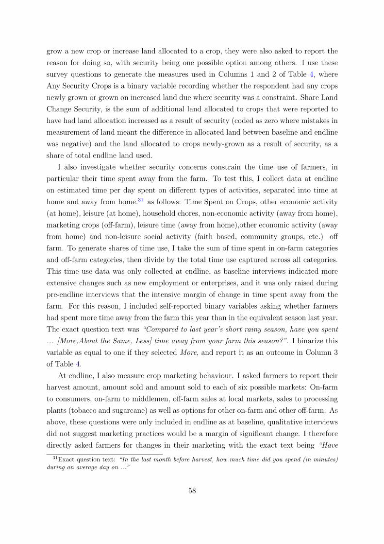
grow a new crop or increase land allocated to a crop, they were also asked to report the

reason for doing so, with security being one possible option among others. I use these

survey questions to generate the measures used in Columns 1 and 2 of Table 4, where

Any Security Crops is a binary variable recording whether the respondent had any crops

newly grown or grown on increased land due where security was a constraint. Share Land

Change Security, is the sum of additional land allocated to crops that were reported to

have had land allocation increased as a result of security (coded as zero where mistakes in

measurement of land meant the difference in allocated land between baseline and endline

was negative) and the land allocated to crops newly-grown as a result of security, as a

share of total endline land used.

I also investigate whether security concerns constrain the time use of farmers, in

particular their time spent away from the farm. To test this, I collect data at endline

on estimated time per day spent on different types of activities, separated into time at

home and away from home.31 as follows: Time Spent on Crops, other economic activity

(at home), leisure (at home), household chores, non-economic activity (away from home),

marketing crops (off-farm), leisure time (away from home),other economic activity (away

from home) and non-leisure social activity (faith based, community groups, etc.) off

farm. To generate shares of time use, I take the sum of time spent in on-farm categories

and off-farm categories, then divide by the total time use captured across all categories.

This time use data was only collected at endline, as baseline interviews indicated more

extensive changes such as new employment or enterprises, and it was only raised during

pre-endline interviews that the intensive margin of change in time spent away from the

farm. For this reason, I included self-reported binary variables asking whether farmers

had spent more time away from the farm this year than in the equivalent season last year.

The exact question text was “Compared to last year’s short rainy season, have you spent

... [More,About the Same, Less] time away from your farm this season?”. I binarize this

variable as equal to one if they selected More, and report it as an outcome in Column 3

of Table 4.

At endline, I also measure crop marketing behaviour. I asked farmers to report their

harvest amount, amount sold and amount sold to each of six possible markets: On-farm

to consumers, on-farm to middlemen, off-farm sales at local markets, sales to processing

plants (tobacco and sugarcane) as well as options for other on-farm and other off-farm. As

above, these questions were only included in endline as at baseline, qualitative interviews

did not suggest marketing practices would be a margin of significant change. I therefore

directly asked farmers for changes in their marketing with the exact text being “Have

31Exact question text: “In the last month before harvest, how much time did you spend (in minutes)during an average day on ...”

58

you changed how much of your harvest you sell away from the farm?” and a follow-up

asking whether they increased or decreased. This variable is binarized, equal to one if

they increased off-farm sales, and reported as Column 4 of Table 4.

To explore whether security influenced the investment behaviour of farmers, I also

collect data on buying and renting of assets. Farmers reported if they had bought or

rented any new assets this year and, if they responded that they had, were asked to list

which assets they had bought or rented from a list of eighteen asset categories. The cat-

egories are as follows: Hip pump, Motorized pump, Hose pipe, Ox-Ploughs, Oxen/work

bulls, Knapsack sprayers, Wheelbarrows, Ox-carts/donkey carts, Hand carts, Zero grazing

unit, Boreholes/wells, Fishing equipment (boats, canoes, etc), Fish pond, Electric gener-

ator, Solar panel, Car battery, Greenhouse, and Water Tank with an option for “Other,

Specify”. I created binarized variables reporting whether the farmer had bought or rented

any assets this year, and included them as Columns 5 and 6 of Table 4.

B.0.4 Value of Agricultural Yield

To measure the value of agricultural production, I aggregate up from the yield for each

crop. I first clean up the crop yields at the individual level, and restrict to observations

where the farmer allocates a non-negligible amount of their land (> 0.25% of their land)

and where there are at least 25 yield observations for that crop. Yields are winsored

within-crop at the highest 2.5%. To find a consistent price for each crop, in order to

aggregate, I use the median sale price across all markets for each crop and multiply this

price by the yield. These crop-level yield values are used for the cropwise regressions

in Appendix Table A7. I then aggregate these crops up to the farm level by taking the

weighted mean income per acre within the three categories Opprtunistic, Deliberate and

Nonstealable. Outliers in these farm-level values are then winsored at the highest 2.5%,

to generate the values used in Table 5.

B.0.5 Learning

To understand whether farmers learned and in what ways they learned, I directly asked

survey questions about the reasons for their updated beliefs. I fist ask whether farmers

now value security more than they did at the beginning of the project. The exact text

of the question was “Have you come to value farm security / watchmen more during this

season?” As a follow-up to this question asking whether the farmers had increased their

valuation of security, I then asked for reasons why they had changed their valuation. This

took the form of a multiple-choice question, capturing direct learning about watchman

effectiveness, learning about farm yields for different crops, learning about crop prices,

59

learning about off-farm prices, and learning about the profits they might earn from their

enterprise. This also captures direct information spillovers where non-matched farmers

observed the experience of a matched farmer. Each of these options, as a binary variable

equal to one if the response was selected and equal to zero if the response was not selected

or the respondent reported no learning, is an outcome in Table 6.

B.0.6 Local Conflict

I now explain the details of the measures of local suspicion and conflict reported in

Table 7. Column 1 is a binary indicator for the farmer responding with a four or five

on a five-point scale in agreement to the statement “In the last month before harvest I

was worried my neighbours would interfere with my farm if I wasnt there”. Column 2

is a binary indicator for the farmer responding with a four or five on a five-point scale

in agreement to the statement “In the last month before harvest I was worried strangers

would interfere with my farm if I wasnt there”. Column 3 is a binary variable equal to

one if the respondent answered Yes to the question “In the last month before harvest,

did you have grievances with your neighbours where you didnt bother confronting them

or bringing it to the authorities?” Column 4 is an integer count of disputes in the last

month before harvest, in response to the question “In the last month before harvesting,

did you have disputes with your neighbours about interference on your farm? How many

times in the last month before harvesting?” where the count of disputes is coded as zero

if the respondent answered No to the first question. Column 5 is the integer count of

how many of these disputes were angry, in response to the question “How many of these

disputes involved some form of threat or aggression?”.

60

C Supplementary Tables

Table A1: Other Measures of Perceived Security

(1) (2) (3)Outcome Var High Risk if

Growing DifferentCrops†

High Risk ifGrowing Similar

Crops†

PerceivedLikelihood of Theft

Attempts

Intervention x Endline† -0.256 -0.049 -0.595(0.075)*** (0.040) (0.149)***

Intervention† -0.007(0.042)

Endline† -0.117(0.059)*

Num. Observations 1,154 577 576Non-Matched Mean 0.63 . .Baseline Median 1.00 . 3.00

* p < 0.1; ** p < 0.05; *** p < 0.01† Binary variable, equal to 1 if true, 0 if not.Standard Errors clustered at the village level in parentheses below estimates. Controls for allspecifications: Randomization strata fixed effects. Watchman Matched is an indicator variablefor assignment to the treated group who were matched to a watchman offering farm security atthe subsidized rate. Column 1 is a binary variable indicating whether the respondent selectedeither four or five on a five point scale of theft risk if they had grown different crops to thosearound them. Column 2 isa binary variable indicating whether the respondent selected eitherfour or five on a five point scale of theft risk if they had grown similar crops to those aroundthem. Column 3 is a response on a scale from one to five on the likelihood of opportunistictheft attempts by people passing by their farm.

61

Table A3: Cropwise New/Increase Treatment Effect

Intervention Group† Summary Stats

TreatmentEffect PointEstimate

TreatmentEffectStandardError

TreatmentEffect asshare ofControlMean

ControlMean

Num Ob-servations

Beans .1049*** (.0346) .73 .1437 577Maize .0653* (.0337) .3 .2141 577Kale .0507*** (.0193) .82 .0616 577Cassava .0272 (.0184) .44 .0616 577Tomatoes .0222** (.0113) 3.76 .0059 577Tobacco .0193 (.0165) .94 .0205 577Green Maize .0174 (.014) 1.18 .0147 577Melon .014** (.0072) . 0 577Saga .0138 (.0107) 1.18 .0117 577Cabbage .0115 (.0083) 1.95 .0059 577

* p < 0.1; ** p < 0.05; *** p < 0.01Controls for each specification: Randomization strata fixed effects. Standard Errors clusteredat the village level.This table presents regressions where the binary outcome is whether a respondent listed thatparticular crop as one where they either i) grew it for the first time or grew this variety for thefirst time this year or ii) increased the amount of land allocated to that crop relative to theequivalent season last year.The two crops with the largest reallocations by raw difference between treatment and controlare, Maize and Beans. This is to be expected, as they are the most common crops and hencehave the lowest adjustment costs for a farmer. The other crops with a significant differencebetween intervention group and the control group are Kale, Tomatoes and Melons, all of whichwere identified in a sample of comparable farmers as being among the most theft-constrained.(See Figure 4.)

62

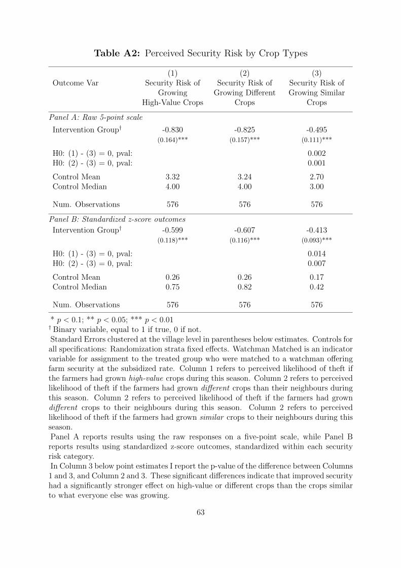
Table A2: Perceived Security Risk by Crop Types

(1) (2) (3)Outcome Var Security Risk of

GrowingHigh-Value Crops

Security Risk ofGrowing Different

Crops

Security Risk ofGrowing Similar

Crops

Panel A: Raw 5-point scale

Intervention Group† -0.830 -0.825 -0.495(0.164)*** (0.157)*** (0.111)***

H0: (1) - (3) = 0, pval: 0.002H0: (2) - (3) = 0, pval: 0.001

Control Mean 3.32 3.24 2.70Control Median 4.00 4.00 3.00

Num. Observations 576 576 576

Panel B: Standardized z-score outcomes

Intervention Group† -0.599 -0.607 -0.413(0.118)*** (0.116)*** (0.093)***

H0: (1) - (3) = 0, pval: 0.014H0: (2) - (3) = 0, pval: 0.007

Control Mean 0.26 0.26 0.17Control Median 0.75 0.82 0.42

Num. Observations 576 576 576

* p < 0.1; ** p < 0.05; *** p < 0.01† Binary variable, equal to 1 if true, 0 if not.Standard Errors clustered at the village level in parentheses below estimates. Controls forall specifications: Randomization strata fixed effects. Watchman Matched is an indicatorvariable for assignment to the treated group who were matched to a watchman offeringfarm security at the subsidized rate. Column 1 refers to perceived likelihood of theft ifthe farmers had grown high-value crops during this season. Column 2 refers to perceivedlikelihood of theft if the farmers had grown different crops than their neighbours duringthis season. Column 2 refers to perceived likelihood of theft if the farmers had growndifferent crops to their neighbours during this season. Column 2 refers to perceivedlikelihood of theft if the farmers had grown similar crops to their neighbours during thisseason.Panel A reports results using the raw responses on a five-point scale, while Panel Breports results using standardized z-score outcomes, standardized within each securityrisk category.In Column 3 below point estimates I report the p-value of the difference between Columns1 and 3, and Column 2 and 3. These significant differences indicate that improved securityhad a significantly stronger effect on high-value or different crops than the crops similarto what everyone else was growing.

63

Table A4: Farm Security - Spillover Check

(1) (2) (3) (4)Outcome Variable Hired

Watchman†Weekshired

watchman

Low FarmSecurity†

Theft risk:High

value†

Intervention x Endline† 0.700 3.697 -0.350 -0.221(0.048)*** (0.292)*** (0.074)*** (0.081)***

Near Intervention Village x Endline† -0.032 -0.121 0.087 0.082(0.048) (0.180) (0.085) (0.096)

Intervention† -0.004 -0.079 -0.021 -0.054(0.012) (0.063) (0.044) (0.054)

Near Intervention Village† -0.005 -0.151 -0.151 -0.099(0.015) (0.093) (0.049)*** (0.062)

Endline† 0.169 0.617 -0.158 -0.135(0.037)*** (0.147)*** (0.053)*** (0.059)**

Non-Matched Mean 0.08 0.28 0.69 0.65Full Sample Baseline Median 0.00 0.00 1.00 1.00

Num. Observations 1,153 1,153 1,153 1,153

* p < 0.1; ** p < 0.05; *** p < 0.01† Binary variable, equal to 1 if true, 0 if not.Standard Errors clustered at the village level in parentheses below estimates. Controls for allspecifications: Randomization strata fixed effects. Watchman Matched is an indicator variablefor assignment to the treated group who were matched to a watchman offering farm security atthe subsidized rate. Near Treated Village indicates whether a control village was less than themedian distance among control villages to a treatment village centroid. Column 1 is a binaryvariable indicating whether the farm had a watchman at all during the study season. Column2 is the number of weeks during this season the watchman was working, equal to zero wherethe farm did not have a watchman. Column 3 is a binary indicator of whether the respondentperceived their farm to have low security, constructed as being equal to one if the respondentselected four or five on a five-point scale and zero otherwise. Column 4 is a similarly binarizedvariable indicating whether the respondent perceived they would have faced a high degree oftheft risk if they had planted high-value crops this season. In addition to perceived theft riskof high-value crops, there is also an effect for other categories of crops.

64

Table A5: Within-Village Spillovers in Perceived Crime

(1) (2))Outcome Var Experienced any crop

theft from farm thisseason†

Crop Theft DecreasedRelative to Last Season†

Intervention Village x Endline† -0.264 0.354(0.076)*** (0.130)**

Num. Observations 65 65

Non-Matched Mean 0.95 0.39

* p < 0.1; ** p < 0.05; *** p < 0.01† Binary variable, equal to 1 if true, 0 if not.Standard Errors clustered in parentheses below estimates.This table reports within-village spillovers in self-reported crime experienced. Here,Watchman Matched x Endline indicates whether a spillover respondent lived in a treat-ment village. These spillover surveys were only conducted at endline while enumeratorswere travelling from household to household in order to conduct surveys with the mainsample. This sample was constructed as a convenience sample within the village. Thepositive effect is suggestive that the presence of the watchmen reduced theft on othernearby farms as well as those assigned to treatment. This indicates that there was someperception that the watchmen nearby would discourage theft more broadly, even if theyweren’t actively protecting another farm.This is suggestive evidence that there are returns to scale and that a watchman inter-vention can impact more than one farm household.

65

C.1 Buying & Renting by Asset

Table A6: Assets Bought & Rented

Panel A: Buying

Asset Name Intervention p-value Control Mean

Water tank .041 .042 .023Ox-Ploughs .04 .085 .029Greenhouse .037 .029 .003Hip pump .036 .002 0Zero grazing unit .032 .015 .003

Panel B: Renting

Asset Name InterventionEffect

p-value Control Mean

Oxen/work bulls -.028 .118 .07Knapsack sprayers -.027 .045 .041Ox-Ploughs -.016 .614 .135Boreholes/wells -.013 .081 .015Water tank -.012 .186 .023

* p < 0.1; ** p < 0.05; *** p < 0.01† Binary variable, equal to 1 if true, 0 if not.Reported p-values are clustered at the village level. Controls for all specifications:Randomization strata fixed effects. Panel A reports the five asset categories withthe largest absolute magnitude of treatment effect on buying, out of a total ofeighteen asset categories. The outcome variable is a binary indicator variableequal to one if the respondent reported buying an asset of this category, equalto zero if the respondent did not select this asset or reported they did not buyany farm assets at all. Panel B is similar to Panel A, but reports the five assetcategories with the largest absolute magnitude of treatment effect on renting.

66

Table A7: Cropwise Income per Acre Treatment Effect

Intervention Group† Crop Characteristics

Coefficient StandardError

HarvestWindow

HarvestingTime

Theft ofOpportu-

nityIndex

Panel A: Low Expected Theft

Millet 16812 (10343)‡ 1 10 -1.027Groundnuts -470 (13255) 2 10 -.879Cassava 10054 (3772)*** 4 10 -.584Sweet potatoes 38742 (24158)‡ 1 7 -.415Beans 9406 (5560)* 1 5 -.007

Panel B: High Expected Theft

Green Maize -1126 (8598) 2 5 .141Banana/plantain 94408 (99111) 3 5 .288Kale 1657 (6469) 24 3 3.794

Panel C: Low Utility to Thieves

Maize 1679 (1671) 1 5 .Sugarcane -17757 (29322) 3 .Tobacco 17858 (26482) 12 6 .

‡ p ≤ 0.15; * p < 0.1; ** p < 0.05; *** p < 0.01Here I report cropwise results for value of agricultural output per farmed acre. These cropwiseresults are aggregated to generate the yield effects reported in Table 5.The characteristics in the right panel show the crop characteristics that are perceived to berelated to ease of theft, and thus form the breakdown of crops into the three categories I use inTable 5.Value of agricultural production is constructed by restricting to crops with at least 25 observa-tions where the crop’s land allocation is at least 0.25% of the farm’s total land allocation thisseason. Individual farm yields are winsored by crop at the highest 2.5%. Using these per-acreyields, total output is generated by multiplying cleaned yield by reported acres allocated tothe crop, and total value of output is generated by multiplying this output by the median self-reported sale price (across all market categories) by crop. In Column 1, total value per acre isgenerated by taking the sum of the value of all crops (constructed as described above) dividedby the sum of land allocated to all included crops, where allocated land share is at least 2.5%and with at least 25 observations. In Columns 2-4 I aggregate production separately by cropshaving characteristics. First, I designate crops that are not consumed directly by households(Tobacco and Sugarcane) and ubiquitous crops (Maize) as Low Utility to Thieves as these areunlikely to be targets of theft. The remaining potential crops are then split into High ExpectedThefts and Low Expected Theft theft crops. High Expected Theft are defined as the potentialcrops above median in an Opportunity for Theft Index defined over potential crops as increasingin the Length of Harvest Window, and decreasing in Minutes Required to Harvest one Kilo-gram. Low Expected Theft Crops are defined as those below median for potential crops in thisOpportunity for Theft Index.

67

Table A8: Pre-Registered Outcome Indices

(1) (2) (3)Outcome Var Cropping

Patterns1

Off Farm TimeUse2

Prices & MarketInteraction3

Panel A: Diff-in-Diff Specification

Intervention x Endline† 0.266 0.282 0.138(0.151)* (0.148)* (0.077)*

FWER p-value [0.17] [0.17] [0.17]

FDR p-value [0.19] [0.19] [0.19]

Intervention† -0.024 -0.051(0.097) (0.107)

Endline† 0.618 0.000(0.092)*** (0.085)

Control Mean 0.31 0.00 0.00Control Median 0.04 -0.31 -0.17

Num. Observations 1,153 1,153 576

Panel B: ANCOVA (Baseline as Controls) Specification

Intervention x Endline† 0.260 0.242 0.139(0.126)** (0.081)*** (0.077)*

FWER p-value [0.02] [0.02] [0.12]

FDR p-value [0.08] [0.01] [0.08]

Control Mean 0.00 0.00 -0.00Control Median -0.11 -0.26 -0.18

Num. Observations 577 577 577

* p < 0.1; ** p < 0.05; *** p < 0.01† Binary variable, equal to 1 if true, 0 if not.Standard Errors clustered at the village level in parentheses below estimates. P-values for multiple

hypothesis corrected tests are reported in square brackets below point estimates. FWER p-value referto the Family-Wise Error Rate method, and FDR p-values refer to the False Discovery Rate method.Both tests computed with one thousand iterations. Controls for all specifications: Randomization stratafixed effects. Watchman Matched is an indicator variable for assignment to the treatment group. PanelA reports results using the more conservative differences-in-differences specification. Panel B reportsresults using the ANCOVA specification discussed in McKenzie (2012).1 Cropping Patterns Index. Combined index of variables indicating change in cropping patterns. SeeTable A9 for results for the individual component variables.2 Off Farm Time Use Index. Combined index of variables indicating more time spent off-farm. SeeTable A10 for results for the individual component variables.3 Prices & Market Interaction Index. Combined index of variables indicating greater market interaction

for crop sales. See Table A11 for results for the individual component variables.

68

Table A9: Components: Cropping Patterns Index

(1) (2) (3) (4) (5) (6) (7) (8) (9)Outcome Var New

CropsLandShare

AnyNew

Crops†

TheftProneLandShare

AnyTheftProneCrops

†

HighlyTheftProneLandShare

MeanTheftRisk

LandUse

Change

LandShareSec.

Crops

Num.Sec.

Crops

Interventionx Endline†

-0.006 0.028 -0.012 -0.016 -0.008 0.008 0.153 0.137 0.437(0.064) (0.077) (0.028) (0.065) (0.026) (0.090) (0.169) (0.042)*** (0.139)***

Intervention† 0.019 -0.004 0.000 -0.019 -0.002 -0.033(0.034) (0.042) (0.019) (0.049) (0.016) (0.056)

Endline† 0.140 0.192 0.126 0.227 0.106 0.350(0.039)*** (0.048)*** (0.018)*** (0.044)*** (0.018)*** (0.057)***

Observations 1,151 1,153 1,151 1,153 1,151 1,151 577 577 577Non-Matched Mean .15 .29 .14 .46 .12 -1.21 .55 .09 .26

* p < 0.1; ** p < 0.05; *** p < 0.01† Binary variable, equal to 1 if true, 0 if not.Standard Errors clustered at the village level in parentheses below estimates. Controls for all specifications: Random-ization strata fixed effects. Watchman Matched is an indicator variable for assignment to the treated group who werematched to a watchman offering farm security at the subsidized rate.The outcome in Column 1, New Crops Land Share, is the share of land the farmer allocated to new crops they hadnever grown before. In Column 2, Any New Crops, is a binary variable that records whether the farmer grew anycrops they had never grown before. In Column 3, Theft-Prone Land Share, is the share of land the farmer allocatedto crops classified as theft-prone, defined as crops that are above-median in the ranking of theft-riskiness measured byan index of objective characteristics. Column 4, Any Theft Prone Crops, is a binary variable that records whether thefarmer grew any crops classified as theft-prone, defined as crops that are above-median in the ranking of theft-riskinessmeasured by an index of objective characteristics. Column 5, Highly Theft Prone Land Share, is the share of land thefarmer allocated to crops classified as highly theft-prone, defined as crops that are above the seventy-fifth percentilein the ranking of theft-riskiness measured by an index of objective characteristics. Column 6, Mean Theft Risk, isthe land share-weighted mean of standardized theft-riskiness scores of crops grown by the farmer. Column 7, LandUse Change, is the total percentage of baseline land that was reallocated to a different crop at endline. Column 8,Land Share to Security-Constrained Crops, is the total share of land allocated to crops that the farmer identified assecurity-constrained, which they either began growing for the first time or to which they allocated additional land,due to security. Column 9, Number of Security-Constrained Crops, is the count of crops that the farmer identified assecurity-constrained, which they either began growing for the first time or to which they allocated additional land, dueto security.

69

Table A10: Components: Time Use Index

(1) (2) (3) (4)Outcome Var Any Off-Farm

Enterprise†Any Off-FarmEmployment†

Share ofReported

Time SpentOff Farm

Spent MoreTime

Off-Farm†

Interventionx Endline†

0.012 0.043 0.015 0.119(0.049) (0.041) (0.010) (0.032)***

Intervention† -0.017 -0.022(0.045) (0.037)

Endline† -0.334 -0.132(0.033)*** (0.030)***

Observations 1,153 1,153 576 577Non-Matched Mean .18 .1 .45 .16

* p < 0.1; ** p < 0.05; *** p < 0.01† Binary variable, equal to 1 if true, 0 if not.Standard Errors clustered at the village level in parentheses below estimates. Controls forall specifications: Randomization strata fixed effects. Watchman Matched is an indicatorvariable for assignment to the treated group who were matched to a watchman offeringfarm security at the subsidized rate.In Column 1 the outcome, Any Off-Farm Enterprise, is a binary variable recordingwhether the farmer had any off-farm enterprise during this season. In Column 2, AnyOff-Farm Employment, records whether the farmer had any off-farm employment (casualor salaried) during this season. In Column 3, Share of Reported Time Spent Off Farm, isthe share of total reported time use allocated to off-farm economic and social activities.In Column 4, Spent More Time Off-Farm, is a self-reported binary variable recordingwhether the farmer spent more time off-farm this season than the equivalent season lastyear.

70

Table A11: Components: Prices & Market Interaction

(1) (2) (3) (4) (5)Outcome Var Share of

HarvestSold

Share ofCrops SoldOff-Farm

Avg. Shareof Harvest

SoldOff-Farm

PricePremium

above Mean

Sold MoreCrops

Off-Farm†

Intervention† 62.998 -0.029 -8.030 -0.618 0.104(82.085) (0.032) (7.549) (0.627) (0.045)**

Num. Observations 574 574 574 458 577Non-matched Mean 80.08 .39 8.48 .47 .13Control Median 0.56 0.33 0.25 -0.70 0.00

* p < 0.1; ** p < 0.05; *** p < 0.01† Binary variable, equal to 1 if true, 0 if not.Standard Errors clustered at the village level in parentheses below estimates. Controls for allspecifications: Randomization strata fixed effects. Watchman Matched is an indicator variable forassignment to the treated group who were matched to a watchman offering farm security at thesubsidized rate.In Column 1 the outcome Share of Harvest Sold is the percentage (0-100) of harvest that was soldon markets as opposed to self-consumed. In Column 2, Share of Crops Sold Off-Farm measuresthe share of crops grown that had any sales off-farm. Column 3, Avg. Share of Harvest SoldOff-Farm, is the average percent (0-100) of harvests sold off-farm. This is computed by taking theaverage of share of harvest sold off-farm for each crop. Column 4 is the average price premiumrelative to the mean. This is computed by measuring, for each crop, the difference between meanprice received by a farmer for that crop as a share of the mean. This mean deviation by crop isthen averaged to generate an aggregate price premium above the mean. Column 6, Sold MoreCrops Off-Farm, is a binary self-reported variable asking farmers whether they had increased theiroff-farm sales this season relative to the equivalent season in the previous year.

71

Table A12: Trust

(1) (2) (3) (4) (5)Outcome Var Neighbours Chief Other

EthnicGroups

NonNeighbours

Strangers

Interventionx Endline†

0.009 0.186 -0.053 -0.032 -0.057(0.202) (0.186) (0.164) (0.175) (0.156)

Intervention† 0.016 -0.027 -0.033 0.002 -0.015(0.120) (0.097) (0.109) (0.113) (0.108)

Endline† -0.238 -0.665 -0.646 -0.247 -0.278(0.139)* (0.146)*** (0.122)*** (0.119)** (0.091)***

Observations 1,153 1,153 1,153 1,153 1,153Non-Matched Mean 3.03 3.69 2.93 2.74 2.37Baseline Median 3.00 4.00 4.00 3.00 2.00

* p < 0.1; ** p < 0.05; *** p < 0.01† Binary variable, equal to 1 if true, 0 if not.Standard Errors clustered at the village level in parentheses below estimates. Controls for allspecifications: Randomization strata fixed effects. Watchman Matched is an indicator variable forassignment to the treated group who were matched to a watchman offering farm security at thesubsidized rate.All outcomes are self-reported trust reported on a five-point scale, where a higher value indicatesgreater trust. The trust measure in Column 1 refers to the farmers neighbours, In Column 2respondents report their trust in their local chief, in Column 3 respondents report their trust inother ethnic groups in their area, in Column 4 they report trust in non-neighbours within theirvillage and Column 5 refers to strangers passing through their village.

72

Table A13: Relative Trust

(1) (2) (3) (4) (5)Outcome Var Neighbours Non

NeighboursStrangers Other

EthnicGroups

Chief

Intervention Group

x Endline†-0.002 -0.043 -0.067 -0.064 0.175(0.104) (0.090) (0.121) (0.084) (0.142)

Intervention Group† 0.027 0.013 -0.003 -0.022 -0.016(0.063) (0.061) (0.078) (0.059) (0.092)

Endline† 0.177 0.167 0.137 -0.231 -0.250(0.063)*** (0.061)*** (0.086) (0.055)*** (0.110)**

Observations 1,153 1,153 1,153 1,153 1,153Non-Matched Mean 0.08 -0.21 -0.59 -0.02 0.74Baseline Median 0.00 -0.20 -0.40 0.00 0.80

* p < 0.1; ** p < 0.05; *** p < 0.01† Binary variable, equal to 1 if true, 0 if not.Standard Errors clustered at the village level in parentheses below estimates. Controls for allspecifications: Randomization strata fixed effects. Watchman Matched is an indicator variable forassignment to the treated group who were matched to a watchman offering farm security at thesubsidized rate.All outcomes are trust relative to an individual’s mean trust in a given period. Each measure ofself-reported trust reported on a five-point scale, where a higher value indicates greater trust. Togenerate the relative trust for each category in each period, I divide each trust measure by therespondent’s mean trust across these five categories in that period. The trust measure in Column1 refers to the farmers neighbours, In Column 2 respondents report their trust in non-neighbourswithin their village, in Column 3 respondents report their trust in strangers passing through theirvillage, in Column 4 they report trust in other ethnic groups in their area and Column 5 refers totrust in their local chief.

73

Table A14: Neighbour Gift-Giving

Gifts Given Gifts Received

(1) (2) (3) (4)Outcome Var Any Gifts

Given†

Size ofGifts

Givena

ReceivedAny Gifts

†Size ofGiftsa

Intervention Group x Endline† 0.040 195 0.035 24(0.068) (111)* (0.049) (18)

Intervention Group† -0.006 -154(0.037) (104)

Endline† -0.460 -1,015(0.046)*** (73)***

Num. Observations 1,153 1,153 576 576Non-Matched Mean 0.61 664 . .Full Sample Baseline Median 1.00 550 . .

* p < 0.1; ** p < 0.05; *** p < 0.01† Binary variable, equal to 1 if true, 0 if not.a This variable is measured in Kenya Shillings (KES), at 100 KES ≈ 1 USD.Standard Errors clustered at the village level in parentheses below estimates. Controls forall specifications: Randomization strata fixed effects. Watchman Matched is an indicatorvariable for assignment to the treated group who were matched to a watchman offeringfarm security at the subsidized rate.The outcome in column 1 is a binary variable recording whether farmers gave any gifts(in-kind or monetary) to their neighbours. In Column 2, the outcome is the total size ofthese gifts given to neighbours. The outcome in Column 3 is a binary variable recordingwhether farmers received any gifts (in-kind or monetary) from their neighbours. Column4 records the approximate of gifts received, with no gifts received being included as zero.

74

Table A15: Institutional Attitudes

(1) (2) (3)Outcome Var Trust in Chief Legitimacy of

FormalPunishment

Perceived ChiefCompetence

Intervention Group x Endline† 0.186 0.038 0.032(0.186) (0.146) (0.155)

Intervention Group† -0.027 0.068 -0.011(0.097) (0.083) (0.080)

Endline† -0.665 -0.475 -0.532(0.146)*** (0.090)*** (0.085)***

Num. Observations 1,153 1,153 1,153Non-Matched Mean 3.69 4.12 3.84Full Sample Baseline Median 4.00 5.00 4.00

* p < 0.1; ** p < 0.05; *** p < 0.01† Binary variable, equal to 1 if true, 0 if not.Standard Errors clustered at the village level in parentheses below estimates. Controls forall specifications: Randomization strata fixed effects. Watchman Matched is an indicatorvariable for assignment to the treated group who were matched to a watchman offeringfarm security at the subsidized rate.Column 1 is self-reported trust in the local chief, reported on a five-point scale wherehigher values indicate stronger trust. Column 2 reports agreement with the statement “Ifsomeone does something bad to you, you should go to legal authorities instead of personalretaliation” on a five-point scale, with 1 being Strongly Disagree and 5 being StronglyAgree. Column 2 is self-reported agreement with the statement “My local chief has beendoing a good job enforcing property rights and punishing thieves” on a five-point scale,with 1 being Strongly Disagree and 5 being Strongly Agree.

75

Table A16: Crime and Theft Attitudes

(1) (2) (3)Outcome Var Agree/Disagree:

Theft acceptable ifyou need food

Agree/Disagree:Theft acceptable ifsomeone has better

harvest

Agree/Disagree:Theft Acceptable ifsomeone earns much

more than you

Intervention Group† -0.062 -0.049 -0.102(0.096) (0.089) (0.089)

Num. Observations 576 576 576Non-matched Mean 1.79 1.72 1.69Control Median 2.00 1.00 1.00

* p < 0.1; ** p < 0.05; *** p < 0.01† Binary variable, equal to 1 if true, 0 if not.Standard Errors clustered at the village level in parentheses below estimates. Controls for allspecifications: Randomization strata fixed effects. Watchman Matched is an indicator variablefor assignment to the treated group who were matched to a watchman offering farm security atthe subsidized rate. The outcomes in this table were only recorded at endline, so the WatchmanMatched variable is the treatment coefficient of interest. Column 1 records a score for agreementon a five-point scale that theft is acceptable in the hypothetical situation that you needs food.Column 2 records a score for agreement on a five-point scale that theft is acceptable in thehypothetical situation that you steal from someone who has a better harvest. Column 3 recordsa score for agreement on a five-point scale that theft is acceptable in the hypothetical situationthat you steal from someone who earns much more than you.

76

Table A17: Security Patrols by Chief

Any Patrols

in Last Month†

More thanTwo Patrols

in Last Month†

(1) (2) (3) (4)

Intervention Group x Endline† -0.093 -0.111 0.028 0.019(0.077) (0.077) (0.061) (0.060)

Intervention Group† 0.075 0.075 -0.007 -0.007(0.055) (0.055) (0.042) (0.042)

Endline† -0.059 -0.052 -0.068 -0.065(0.047) (0.047) (0.038)* (0.038)*

Spillover Household† 0.006 -0.067 0.017 -0.018(0.053) (0.072) (0.044) (0.052)

Intervention Village x

Spillover Household†0.173 0.083

(0.091)* (0.084)

Num. Observations 1,031 1,031 1,031 1,031Non-Matched Mean 0.39 0.39 0.39 0.39

* p < 0.1; ** p < 0.05; *** p < 0.01† Binary variable, equal to 1 if true, 0 if not.Standard Errors clustered at the village level in parentheses below estimates. Controlsfor all specifications: Randomization strata fixed effects.In Columns 1 and 2, the outcome is a binary variable indicating whether the respondentobserved any security patrols by their local chief in the last month before harvest. InColumns 3 and 4, the outcome is a binary variable indicating more intensive patrols,whether the chief conducted at least two patrols in the last month before harvest.

77

D Supplementary Figures

Figure A1: Experiment Location Within Kenya

Description: Map showing experiment location (Migori) relative to nearby major population centres in Kenya.

Figure A2: Sample Villages around Migori Town

Description: This map shows the centroids of treated and control village around Migori town centre.

78

Figure A3: Watchman Recruitment Map

Description: This map shows the locations of watchmen recruitment meetings. Recruitment took place in thenorth, near the city of Narok, where underemployed young people often go looking for work, and in the southof Maasailand near the game reserves, where underemployed young people also go looking for work in thetourism sector.

79

Figure A4: Typical Plot Boundary

Description: This figure shows that where plots are not demarcated by a natural boundary like a river or road,they are clearly demarcated by a man-made boundary such as the hedgerow at the edge of the maize field inthe photo above.Data Source: Author’s own photograph.

80

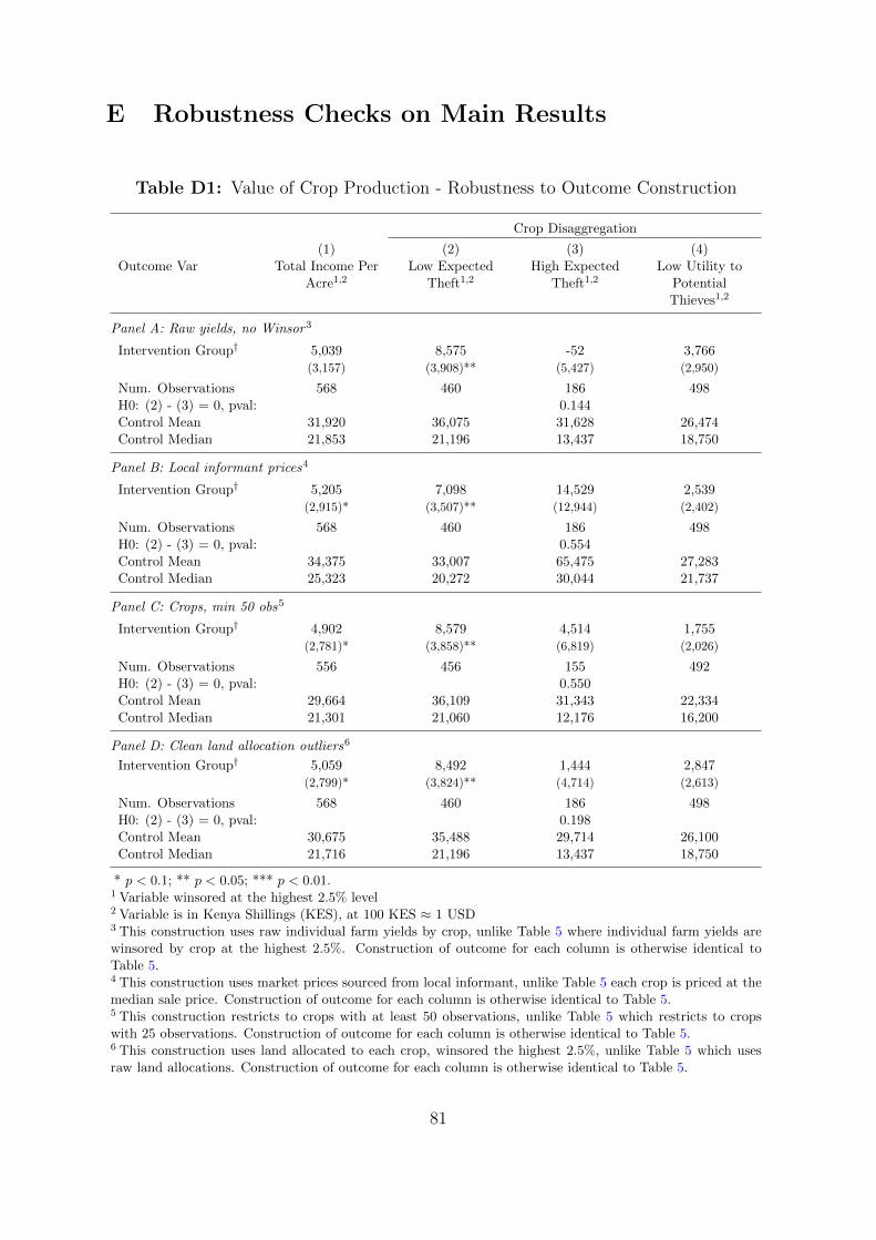
E Robustness Checks on Main Results

Table D1: Value of Crop Production - Robustness to Outcome Construction

Crop Disaggregation

(1) (2) (3) (4)Outcome Var Total Income Per

Acre1,2Low Expected

Theft1,2High Expected

Theft1,2Low Utility to

PotentialThieves1,2

Panel A: Raw yields, no Winsor3

Intervention Group† 5,039 8,575 -52 3,766(3,157) (3,908)** (5,427) (2,950)

Num. Observations 568 460 186 498H0: (2) - (3) = 0, pval: 0.144Control Mean 31,920 36,075 31,628 26,474Control Median 21,853 21,196 13,437 18,750

Panel B: Local informant prices4

Intervention Group† 5,205 7,098 14,529 2,539(2,915)* (3,507)** (12,944) (2,402)

Num. Observations 568 460 186 498H0: (2) - (3) = 0, pval: 0.554Control Mean 34,375 33,007 65,475 27,283Control Median 25,323 20,272 30,044 21,737

Panel C: Crops, min 50 obs5

Intervention Group† 4,902 8,579 4,514 1,755(2,781)* (3,858)** (6,819) (2,026)

Num. Observations 556 456 155 492H0: (2) - (3) = 0, pval: 0.550Control Mean 29,664 36,109 31,343 22,334Control Median 21,301 21,060 12,176 16,200

Panel D: Clean land allocation outliers6

Intervention Group† 5,059 8,492 1,444 2,847(2,799)* (3,824)** (4,714) (2,613)

Num. Observations 568 460 186 498H0: (2) - (3) = 0, pval: 0.198Control Mean 30,675 35,488 29,714 26,100Control Median 21,716 21,196 13,437 18,750

* p < 0.1; ** p < 0.05; *** p < 0.01.1 Variable winsored at the highest 2.5% level2 Variable is in Kenya Shillings (KES), at 100 KES ≈ 1 USD3 This construction uses raw individual farm yields by crop, unlike Table 5 where individual farm yields arewinsored by crop at the highest 2.5%. Construction of outcome for each column is otherwise identical toTable 5.4 This construction uses market prices sourced from local informant, unlike Table 5 each crop is priced at themedian sale price. Construction of outcome for each column is otherwise identical to Table 5.5 This construction restricts to crops with at least 50 observations, unlike Table 5 which restricts to cropswith 25 observations. Construction of outcome for each column is otherwise identical to Table 5.6 This construction uses land allocated to each crop, winsored the highest 2.5%, unlike Table 5 which usesraw land allocations. Construction of outcome for each column is otherwise identical to Table 5.

81

Table D2: Cropwise Income per Acre Treatment Effect

Intervention Group† Crop Characteristics

Coefficient StandardError

HarvestWindow

HarvestingTime

Theft ofOppor-tunityIndex

Panel A: Low Expected Theft

Millet 15961 (9421)* 1 10 -1.027Groundnuts -1327 (12653) 2 10 -.879Cassava 9501 (3557)*** 4 10 -.584Sweet potatoes 38742 (24158)‡ 1 7 -.415Beans 9436 (5229)* 1 5 -.007

Panel B: High Expected Theft

Green Maize 126 (7851) 2 5 .141Banana/plantain 1388 (44863) 3 5 .288Kale 2418 (5919) 24 3 3.794

Panel C: Low Utility to Thieves

Maize 1288 (1492) 1 5 .Sugarcane -15142 (28362) 3 .Tobacco 19894 (24892) 12 6 .

‡ p ≤ 0.15; * p < 0.1; ** p < 0.05; *** p < 0.01 Yield: w5, Price: Med, Obs cutoff: 25Here I report cropwise results for value of agricultural output per farmed acre. These cropwiseresults are similar to those in Table A7, except here I winsor the top 5% instead of the top2.5%, to be sure that outliers are not driving the results.The characteristics in the right panel show the crop characteristics that are perceived to berelated to ease of theft, and thus form the breakdown of crops into the three categories I use inTable 5.Value of agricultural production is constructed by restricting to crops with at least 25 observa-tions where the crop’s land allocation is at least 0.25% of the farm’s total land allocation thisseason. Individual farm yields are winsored by crop at the highest 5%. Using these per-acreyields, total output is generated by multiplying cleaned yield by reported acres allocated tothe crop, and total value of output is generated by multiplying this output by the median self-reported sale price (across all market categories) by crop. In Column 1, total value per acre isgenerated by taking the sum of the value of all crops (constructed as described above) dividedby the sum of land allocated to all included crops, where allocated land share is at least 2.5%and with at least 25 observations. In Columns 2-4 I aggregate production separately by cropshaving characteristics. First, I designate crops that are not consumed directly by households(Tobacco and Sugarcane) and ubiquitous crops (Maize) as Low Utility to Thieves as these areunlikely to be targets of theft. The remaining potential crops are then split into High ExpectedTheft and Low Expected Theft theft crops. High Expected Theft are defined as the potentialcrops above median in an Opportunity for Theft Index defined over potential crops as increasingin the Length of Harvest Window, and decreasing in Minutes Required to Harvest one Kilo-gram. Low Expected Theft Crops are defined as those below median for potential crops in thisOpportunity for Theft Index.

82

F Supplementary Descriptive Evidence

Figure A5: Theft & Experimentation

Description: This figure shows that perceived risk from being a lone adopter of new crops is significantly higherthan when adopting with others.Data Source: Baseline survey with respondents.

Theft is additionally perceived to be particularly focused on those who undertake new or

different activities. This acts as a constraint on farmers who seek to experiment and adopt

new technology on their own. In Figure A5, I show that the risk of theft is perceived to be

significantly stronger for who adopt a new crop on their own compared to those who adopt at

the same time as others. The origins of these beliefs are unclear, but it are possibly related to

the ‘moral economy of the peasant’ as outlined in Scott (1976), where innovation and experi-

mentation in search of greater profits is considered immoral. This morality rule is derived from

an emphasis on preventing catastrophe over trying to increase expected profits. In Platteau

(2014) we see a historical example of a redistributive constraint that binds for innovators. He

documents how upwardly mobile individuals freed themselves from local redistributive norms

by converting to Islam as an obvious signal that they had opted out of the local culture and as-

sociated reciprocal obligations. These examples are consistent with the expectations of farmers

in this sample regarding how their neighbours may respond to someone who is taking risks to

experiment with adoption of technology that may increase their income.

83