Embed Size (px)
Citation preview

The Functional Organisation and Role in
Visually Guided Behaviour of the Top-Down
Projection from Anterior Cingulate Cortex to
Primary Visual Cortex
Eluned Broom
A thesis submitted for the degree of PhD in Neuroscience
Cardiff School of Biosciences
Cardiff University
June 2019

i
Summary
The interplay between bottom-up and top-down projections help the brain to build a
perception of the visual world. Top-down projections, in particular, are believed to
influence perception using previous experience and current context. One way in which
they do this is in the direction of visual attention. Anterior cingulate cortex (ACC), a
structure from which top-down projections are believed to emanate from, has been
implicated in tasks requiring visual attention. Furthermore, studies in mice have shown
an attentional-like effect in primary visual cortex (V1) neurons when a projection
originating from ACC and terminating at V1 was artificially stimulated using
optogenetics. The aim of the following studies was to determine whether ACC
influenced the direction of visual attention under endogenous conditions.
To do this, two main approaches were taken. First, the functional organisation of ACC
axons in V1 were compared to layer 2/3 V1 pyramidal neurons in order to investigate
whether the two populations were retinotopically matched. Secondly, the activity of
ACC axons during a visually guided discrimination task was examined to discern
whether it was elevated when mice performed well. This was achieved using calcium
sensitive genetic indicators including gCaMP6s and jrGECO1a to record neuronal
activity while awake, behaving, head-restrained mice completed visual tasks. To
investigate functional organisation, a retinotopic protocol was run where mice passively
viewed gratings in 36 separate locations. The visual discrimination task consisted of a
reward-based go/no-go structure.
It was found that significantly fewer ACC axons exhibited spatially specific responses
than layer 2/3 V1 neurons. As well as this, instead of retinotopically matching layer 2/3
V1 neurons, ACC axons lying superficially to them relayed information about a wider

ii
area of visual space in both azimuth and elevation. Although some ACC axons showed
orientation selectivity, grouping them by the orientation preference did not result in any
retinotopic matching. Together, these results demonstrated that ACC axons do not
appear to be as visually responsive as or retinotopically matched to layer 2/3 V1 somas
in the same location in V1 under passive conditions.
As well as this, it was found that ACC activity was not greater when mice performed
trials correctly compared to incorrectly in visually guided tasks. This elevated activity
appeared to occur during the response phase of the task and, in particular, in trials
where mice carried out the motor response of licking. Taken together, these data
suggested the neural projection from ACC to V1 was not involved directly in the
perception of the visual stimulus, even when its onset could be predicted, and was
instead associated with the motor response of the animal. On top of this, the activity of
a fraction of these ACC axons appeared to be modulated by the addition of a reward.
Overall, the data presented here indicates that the ACC projection to V1 is involved in
visually guided tasks but is associated more with the motor response of licking than the
perception of the visual stimulus. The additional modulation by reward suggests that
this association depends upon the outcome of trials and may therefore be important for
behaviours such as reward timing.

iii
Acknowledgements
The work presented in this thesis is my own but would not have been possible if not for
all those who supported me throughout my PhD.
Firstly, I would like to thank my supervisors Prof. Frank Sengpiel and Dr Adam Ranson
who guided me through each of the studies. They were both helpful and critical,
allowing me to develop as a scientific researcher. Adam, especially, helped with
teaching and giving advice on the techniques and analysis used throughout my thesis. I
would also like to thank other members of the lab including Dr Richard Inman, who
helped to develop the behavioural task, as well as Fangli Chen, who helped me carry
out the detection task as well as providing mangoes.
I could not have asked for more supportive friends. I would like to especially thank
Nicole Pacchiarini, Annelies de Haan, Richard Ludlow and Harley Worthy for always
being up for coffee or a run whenever it was needed. Last, but by no means least, I
would like to thank my family for their unwavering belief in me.

1
Contents
1 General Introduction .............................................................................................. 6
1.1 Introduction into bottom-up and top-down processing ..................................... 6
1.2 Bottom-up projections in the visual system ..................................................... 8
1.2.1 From the eye to primary visual cortex ...................................................... 8
1.2.2 The structure and classical visual properties of V1 neurons in mice ...... 11
1.2.3 Higher visual areas in mice .................................................................... 17
1.3 Top-down influences on the visual system .................................................... 20
1.3.1 Top-down modulation of V1 neurons during locomotion ........................ 21
1.3.2 Top-down modulation of V1 during visual attention ................................ 22
1.3.3 Predictive coding as an explanation for visual perception ...................... 25
1.3.4 An imbalance in top-down and bottom-up processing can result in
neuropsychiatric conditions such as schizophrenia .............................................. 27
1.4 The top-down influence of ACC upon V1 ...................................................... 29
1.4.1 The structure and function of ACC lends itself to maintaining and
updating representations ..................................................................................... 29
1.4.2 Projection profile of ACC neurons in mice.............................................. 31
1.4.3 Impact of top-down projections on V1 in mice ........................................ 35
1.5 Use of two-photon imaging of calcium sensitive indicators ........................... 39
1.6 Aims of the study ............................................................................................... 41
2 Materials and Methods ........................................................................................ 42
2.1 Animals......................................................................................................... 42
2.2 Viral Injection and Cranial Window Implant ................................................... 42
2.3 Intrinsic Signal Imaging ................................................................................. 44
2.4 Two-Photon Imaging..................................................................................... 47
2.5 Visual Stimuli ................................................................................................ 47
2.6 Calcium Imaging Data Analysis .................................................................... 47
3 Functional Organisation of Anterior Cingulate Cortex and Lateral Medial Cortex
Axons Terminating in Primary Visual Cortex ............................................................... 52
3.1 Introduction ................................................................................................... 52
3.1.1 Properties of V1 neurons and modulation during contexts requiring top-
down processing .................................................................................................. 52
3.1.2 Input from ACC ...................................................................................... 54
3.1.3 Input from lateral medial cortex of visual cortex ..................................... 54
3.1.4 Aims of this study .................................................................................. 55
3.2 Materials and Methods ................................................................................. 57
3.2.1 Mice ....................................................................................................... 57

2
3.2.2 Viral Injection and Cranial Window Implant ............................................ 57
3.2.3 Two-Photon Imaging ............................................................................. 61
3.2.4 Visual Stimulus Protocol ........................................................................ 61
3.2.5 Analysis ................................................................................................. 62
3.3 Results ......................................................................................................... 68
3.3.1 Receptive Field Properties of ACC Axons Compared to V1 Somas ....... 68
3.3.2 Receptive Field Scatter of LM Axons Compared to V1 Somas .............. 76
3.3.3 Receptive Field Offset of ACC and LM Axons from V1 Somas .............. 80
3.3.4 Experience-dependent properties of LM axon organisation ................... 86
3.3.5 Functional organisation of ACC RFCs compared to V1 somas RFCs is
not dependent on orientation selectivity ............................................................... 96
3.4 Summary of Findings .................................................................................. 102
4 The Involvement of Anterior Cingulate Cortex Axons Terminating in Primary Visual
Cortex in Visually Guided Tasks ............................................................................... 103
4.1 Introduction ................................................................................................. 103
4.2 Materials and Methods ............................................................................... 107
4.2.1 Mice ..................................................................................................... 107
4.2.2 Viral Injection and Cranial Window Implant .......................................... 107
4.2.3 Intrinsic Signal Imaging ........................................................................ 108
4.2.4 Visual Discrimination Task ................................................................... 108
4.2.5 Visual Detection Task .......................................................................... 113
4.2.6 Perfusion and Histology ....................................................................... 114
4.2.7 Data Analysis of Neuronal Activity ....................................................... 114
4.3 Results ....................................................................................................... 116
4.3.1 Learning a retinotopically predictable go/no-go visual discrimination task
116
4.3.2 The activity of ACC axons was elevated during specific time windows
during the go/no-go discrimination ..................................................................... 119
4.3.3 Elevated activity in ACC axons is not linked to improved performance 124
4.3.4 Increasing the task difficulty did not alter ACC circuit recruitment ........ 128
4.3.5 Detection task and multi-colour labelling .............................................. 136
4.3.6 Association of ACC activity and lick activity ......................................... 144
4.3.7 ACC activity is associated with reward processing .............................. 150
4.4 Summary of Findings .................................................................................. 153
5 General Discussion ............................................................................................ 154
5.1 Summary of Studies ................................................................................... 154
5.2 Functional Organisation of anterior cingulate cortex and lateral medial cortex
axons terminating in primary visual cortex ............................................................. 154

3
5.2.1 ACC axons lack retinotopic organisation but over-represent the horizontal
plane relative to V1 somas in the same retinotopic location in V1 ...................... 154
5.2.2 LM axons show retinotopic organisation and over-represent the area of
visual space binocular to V1 somas in the same retinotopic location in .............. 155
5.3 The involvement of anterior cingulate cortex axons terminating in primary
visual cortex in visually guided tasks ..................................................................... 160
5.3.1 There are more active ACC axons during correct go trials than in correct
no-go trials ......................................................................................................... 161
5.3.2 ACC axons that discriminate between correct and incorrect trials show
elevated activity during correct go and incorrect no-go trials .............................. 162
5.3.3 General elevated activity is not observed when the visual discrimination
task is more difficult ........................................................................................... 163
5.3.4 Changing the task and stimulus properties did not result in an attentional
signal 164
5.3.5 ACC axon activity is associated with the lick behavioural response ..... 165
5.3.6 ACC axon activity is influenced by reward ........................................... 166
5.3.7 Further study into the role of the ACC to V1 projection in visually guided
tasks 167
5.3.8 Methodological drawbacks of the techniques used .............................. 169
5.3.9 Concluding remarks ............................................................................. 170
6 References ........................................................................................................ 171

4
List of Figures
Figure 1.1: Schematic of the mouse visual system ..................................................... 10
Figure 1.2: Excitatory neurons in V1 ........................................................................... 12
Figure 1.3: Reciprocal projection between ACC and V1 ............................................. 13
Figure 1.4: Structure within V1 .................................................................................... 15
Figure 1.5: Arrangement of higher visual areas (HVAs) in visual cortex ...................... 19
Figure 1.6: Optical illusions indicating the necessity of internal representations to
interpret visual stimuli ................................................................................................. 20
Figure 1.7: Schematic of predictive coding model ....................................................... 26
Figure 1.8: The density profile of ACC projections ...................................................... 33
Figure 1.9: Artificial stimulation of ACC neurons via optogenetics projecting to V1 leads
to attentional effects (adapted from Zhang et al., 2014) .............................................. 38
Figure 2.1: Intrinsic signal imaging to identify areas of visual cortex ........................... 46
Figure 2.2: Example of axonal labelling and detection ................................................ 50
Figure 2.3: Example of axonal and soma labelling over multiple planes ...................... 51
Figure 3.1: Injection sites of gCaMP6s ........................................................................ 60
Figure 3.2: Schematic of the retinotopy protocol ......................................................... 62
Figure 3.3: Example fluorescence traces extracted from ACC axons .......................... 63
Figure 3.4: Example fluorescence traces extracted from V1 somas ............................ 64
Figure 3.5: Example of neuronal responses and the two-dimensional Gaussian fit ..... 66
Figure 3.6: A proportion of ACC axons are visually responsive ................................... 69
Figure 3.7: ACC axons show retinotopic preferences ................................................. 71
Figure 3.8: ACC axons carry signals from a wider area of visual space than V1 somas
process in the same area of visual cortex. .................................................................. 73
Figure 3.9: The distribution of V1 soma and ACC axon RFCs across visual space in
which visual stimuli were presented ............................................................................ 75
Figure 3.10: LM axons show retinotopic preferences .................................................. 77
Figure 3.11: LM axons carry signals from a wider area of visual space in elevation than
V1 somas process in the same area of visual cortex .................................................. 79
Figure 3.12: ACC axon RFCs are offset in the horizontal plane compared to V1 somas
RFCs .......................................................................................................................... 82
Figure 3.13: LM axon RFCs are offset in the binocular direction compared to V1 somas
RFCs .......................................................................................................................... 84
Figure 3.14: Dark reared experiment .......................................................................... 87
Figure 3.15: Example RFCs for one dark reared mouse for each imaging session ..... 91
Figure 3.16: Scatter of LM axons and V1 soma RFCs after dark rearing .................... 92
Figure 3.17: Mean V1 soma and LM axon RFCs for dark reared mice ........................ 93
Figure 3.18: LM axon RFC offset from V1 soma mean RFCs is not in the direction of
the binocular zone after dark rearing........................................................................... 94
Figure 3.19: ACC axons show orientation selectivity but there is not an over-
representation of cardinal orientation preference ........................................................ 97
Figure 3.20: Orientation-dependent organisation of ACC axon RFC offset from V1
somas ....................................................................................................................... 100
Figure 3.21: Organisation of ACC axon offset values relative to their orientation
preferences ............................................................................................................... 101
Figure 4.1: Stage one of the visual discrimination task ............................................. 109
Figure 4.2: Stage two of the visual discrimination task .............................................. 111
Figure 4.3: Mice can perform a go/no-go visual discrimination task .......................... 118
Figure 4.4: ACC injection and cranial window implant ............................................... 120
5
Figure 4.5: ACC axon activity during the retinotopically predictable version of the task
................................................................................................................................. 123
Figure 4.6: Elevated activity in ACC axons is not associated with increased
performance in a visual discrimination task ............................................................... 127
Figure 4.7: Animals can learn a more difficult, retinotopically unpredictable variant of
the visual discrimination task .................................................................................... 129
Figure 4.8: Axons respond preferentially to the go stimulus regardless of where the
stimulus is, and this response is from the same population of axons ........................ 131
Figure 4.9: The more difficult retinotopically unpredictable version of the visual
discrimination task did not recruit ACC axons for improved performance .................. 133
Figure 4.10: The retinotopically unpredictable task with lower contrast variant of the
task does not recruit ACC axons ............................................................................... 135
Figure 4.11: Mice are able to learn a visual detection task ........................................ 137
Figure 4.12: V1 soma and ACC axon response when stimulus is presented inside the
receptive field ........................................................................................................... 140
Figure 4.13: V1 soma and ACC axon response when stimulus is presented outside the
receptive field ........................................................................................................... 143
Figure 4.14: ACC activity is linked to lick response before any learning has occurred
................................................................................................................................. 145
Figure 4.15: Correlation of ACC axon neural activity and lick frequency ................... 146
Figure 4.16: Cross Correlation of ACC axon neural activity and lick activity .............. 148
Figure 4.17: ACC activity is linked to locomotion....................................................... 149
Figure 4.18: ACC axon neural activity is associated with reward .............................. 151
Figure 5.1: A schematic of the theoretical network involved in the prediction of object
movement by LM ...................................................................................................... 158

6
1 General Introduction
1.1 Introduction into bottom-up and top-down processing
The brain is a complex organ made up of an abundance of multifarious connections.
The synergy of these allows it to interact with and interpret a vast number of stimuli
from the outside world. To achieve this, two processing streams referred to as bottom-
up and top-down, are used. Bottom-up processing involves detecting stimuli in the
external world. It is, however, both impossible and undesirable to process information
about the entire sensory environment at once and so top-down projections, which
originate from within the brain itself, work to modulate sensory perception based on
current context and previous experience. Each system must work dynamically to meet
the demands of the current situation (Desimone and Duncan, 1995), and an imbalance
between the two can lead to neuropsychiatric disorders such as schizophrenia (Friston,
1998).
Since the introduction of the concepts of bottom-up and top-down processing, their
relative influence upon visual perception has been debated. The idea that visual
perception is solely based on information carried by bottom-up processes, that are in
turn driven directly by the sensory environment, was purported by Gibson’s ecological
theory of visual perception (Gibson, 1966; Gibson, 1979; Goldstein, 1981). This theory
asserts that the dynamic optic array of light that reaches the eye is sufficient for the
observer to interpret the environment without the aid of intervening top-down input.
Integral to this theory is the accurate and efficient perception of invariants in the
sensory environment such as gravity, the separation of two hemispheres of light at the
horizon or the increasing density of optical texture. It cannot, however, explain natural
visual illusions. On the other hand, Gregory (1970) argues for the contribution of top-
down processing to visual perception. This involves the use of higher cognitive
processing to apply past experience or stored knowledge to the interpretation of what is

7
perceived. It involves hypothesis testing, with errors leading to inaccuracies in
perception, such as visual illusions. It is likely that both these systems are utilised. If
faced with an unfamiliar situation, there would be no model on which to build visual
perception and thus bottom-up processing would dominate the formation of visual
perception. When situations gain familiarity, and perception can be based on learned
constructs, this balance would shift to top-down processing.
To build a visual perception of the world from bottom-up and top-down processing,
these streams must be organised so that information can be efficiently integrated and
interpreted. In some instances, this is believed to be via a hierarchical organisation with
bottom-up processing dominating ascending pathways and top-down dominating
descending pathways (Theeuwes, 2010). In other cases, a more dynamic interpretation
has been suggested where each type of processing can occupy ascending or
descending pathways, and the demarcation is instead to do with flexibility in the
information carried (Rauss and Pourtois, 2013). What is common to all approaches,
however, is that bottom-up projections convey signals that faithfully represent the
sensory environment and must thus illicit predictable activity in sensory cortices that
remains robust and consistent regardless of context or learning. On the other hand,
top-down projections need to be flexible so that their activity, and in turn influence, can
change depending on experience and context.
Primary visual cortex (V1) is one site at which bottom-up and top-down projections
converge and thus the influence on neural activity of both can be examined there.

8
1.2 Bottom-up projections in the visual system
The bottom up projection from the eye to V1, and subsequent receptive field properties
observed there, are believed to faithfully relay information about the external
environment to sensory cortices.
1.2.1 From the eye to primary visual cortex
Mice have two eyes positioned laterally resulting in hemi-panoramic vision (Priebe and
McGee, 2014). The visual field of each eye covers both monocular and binocular
locations with an overlap of approximately 40° of observable space (Figure 1.1).
Light hits the eye and travels through the cornea, pupil, lens and vitreous chamber
before reaching rods and cones located at the retina. At this point, the light is converted
into electrical impulses and this signal is carried to retinal ganglion cells (RGCs). As it
is transmitted, it undergoes a filtering process by retinal interneurons including
horizontal, bipolar and amacrine cells which shape the output carried by the RGCs.
There are currently believed to be 33 different types of retinal ganglion cells (Baden et
al., 2016), which each respond to a particular aspect of the visual scene.
From here, the signals are transmitted to a diverse range of targets across the brain.
Visualisation of these projections using cholera toxin B subunit has elucidated that no
less than 46 brain regions are innervated directly by RGCs in the mouse (Morin and
Studholme, 2014), providing visual information to circuits involved in multiple functions
including image formation. One such target is the dorsal lateral geniculate nucleus
(dLGN) which in turn relays information directly to the visual cortex. Other terminals
include the superior colliculus and the pulvinar nuclei.

9
The projection from RGCs to visual cortex via the dLGN is crucial in image formation
and subsequent visual perception. In this pathway, a proportion of RGCs cross
hemispheres at the optic chiasm, the percentage of which is determined by the
binocular visual range. Humans are highly binocular and so only approximately 50% of
RGCs will cross at the optic chiasm. Mice, on the other hand, have a much smaller
binocular range. This results in the majority of RGCs crossing, with only approximately
3-5% remaining on the ipsilateral side (Petros et al., 2008). From here, the RGCs
project to the dLGN where the signals are filtered and modulated and then are
transmitted to primary visual cortex (V1) via the optic radiation.

10
Figure 1.1: Schematic of the mouse visual system
The ipsilateral monocular (blue), contralateral monocular (red) and binocular (purple) visual
fields are shown. Information about the visual scene is collected by the eyes and transmitted
via the dLGN to visual cortex from both the ipsilateral (blue) and contralateral (red) eyes.
Figure adapted from Priebe et al., 2014.

11
1.2.2 The structure and classical visual properties of V1 neurons in mice
Visual cortex, and in particular primary visual cortex (V1), has been extensively studied
across species. It consists of multiple anatomically and functionally distinct regions and
features that together form a hierarchical structure to aid visual perception.
Anatomically, visual cortex resides in a posterior position of the neocortex of the
mouse. Primary visual cortex (V1) lies within the centre of the visual cortex, is
surrounded by higher visual areas (HVAs) identified via intrinsic signal imaging
(Kalatsky and Stryker, 2003; Garrett et al., 2014; Juavinett et al., 2016) and responds
to a broad range of visual stimuli (Andermann et al., 2010). It covers approximately
3mm2 of the neocortex and consists of layers 1-6, with layer 1 being most superficial.
Input from the thalamus is derived predominantly from core-type excitatory neurons
that primarily project to layer 4, although there is also thalamic input to layer 1 (Rubio-
Garrido et al., 2009; Figure 1.2A). V1 additionally receives callosal projections from the
contralateral hemisphere that terminate in layer 1-3 and 5 (Mizuno et al., 2007).
Each layer of mouse cortex is populated with neurons that differ in morphology,
function and projection patterns. One subset of these neurons are excitatory and can
be divided into three main groups (Figure 1.2). Intratelecephalic pyramidal (IT) neurons
are located in layers 2-6 and play the predominant role of receiving input from axons
projecting from the dLGN in layer 4 of visual cortex. These neurons project only in the
telencephalon and extensively connect left and right hemispheres via the corpus
collosum and anterior commissure. Within this group of neurons there are numerous
subtypes identified by their differing locations and projection patterns, something that
may in turn be controlled by their genetic composition (Harris and Shepherd, 2015).
Pyramidal tract (PT) neurons are located in L5B and project to subcerebral destinations
such as the brainstem and spinal cord. Corticothalamic (CT) reside predominantly in
layer 6 and project primarily to the ipsilateral thalamus (Harris and Shepherd, 2015).

12
Figure 1.2: Excitatory neurons in V1
A: Intratelencephalic (IT) neurons that receive input from neurons projecting from the
dLGN of the thalamus reside in layer 4 and project mainly to layer 2/3 of V1. B: IT
neurons also constitute neuronal cell types in layers 2/3, 5 and 6 of V1. C: Pyramidal
tract (PT) neurons are located in layer 5, project to superficial V1 and innervate
subcerebral destinations. D: Corticothalamic (CT) neurons originate in layers 5 and 6 of
V1. Figure adapted from Harris and Shepherd, 2015.

13
From visual cortex, pyramidal neurons project to other structures including ACC.
Retrograde labelling has shown that, in this case, pyramidal neurons project from L2/3
and 5 of ACC to L1 of V1 (Zhang et al., 2014; Zhang et al., 2016; Figure 1.3A-C).
Anterograde tracing using an AAV expressing mCherry injected into V1 has indicated
that there is a reciprocal connection from V1 to ACC (Zhang et al., 2016; Figure 1.3D).
Figure 1.3: Reciprocal projection between ACC and V1
A: Sagittal diagram of a mouse brain indicating the locations of slices shown in B and
C B: Left: The site from an injection of retrograde beads into V1. Right: All the locations
of stained neurons in ACC as a result of the retrograde injection in V1. C: Left: An
injection site at ACC for anterograde staining. Right: The stained neurons in V1
suggesting ACC axons project predominantly to L1 V1. D: Left: The injection site in V1
for anterograde labelling using mCherry. Right: ACC (also referred to as the anterior
cingulate area (ACA)) neurons labelled from the injection of anterograde tracer in V1.
Figure adapted from Zhang et al., 2014 and Zhang et al., 2016.

14
As well as excitatory pyramidal neurons, V1 contains an array of GABAergic
interneurons arranged in a specific circuitry. Parvalbumin positive (PV+) cells strongly
inhibit one another and pyramidal neurons, but provide little to other interneurons,
Somatostatin positive (SST+) neurons are different in that they avoid inhibiting other
SST+ cells and instead target all other populations. Vasoactive Peptide positive (VIP+)
interneurons preferentially inhibit SST+ neurons (Pfeffer et al., 2013; Figure 1.4B). This
system allows for multi-tier modulation of pyramidal neurons, and connectivity across
layers (Jiang et al., 2015; Pakan et al., 2016).

15
Figure 1.4: Structure within V1
A: Mouse V1 is made up of layers 1-6 and receives the majority of input from the thalamus
via the optical radiation, which terminates mainly in layer 4 (adapted from Smith et al., 2008
and shown in more detail in Figure1.2). B: Interneuron networks in V1. VIP+ interneurons
preferentially inhibit SST+ neurons. STT+ interneurons inhibit all other types, including
excitatory pyramidal neurons. PV+ interneurons inhibit themselves as well as STT+ and
pyramidal neurons. The majority of PV+ interneurons are basket cells and make multiple,
large synapses on the proximal dendrites and cell bodies of pyramidal neurons. They are
typically fast-spiking (Callaway, 2016). SST+ interneurons are a prominent source of input to
the apical tufts of pyramidal neurons and possibly regulate feedback and lateral influences
(Callaway, 2016).

16
A major primary functional organisation within V1 is the retinotopic map. Neurons
positioned in medial V1 respond to more monocular areas of visual space, and more
lateral V1 neurons represent binocular areas of central visual space. As well as this,
anterior and posterior V1 respond to stimuli lower and higher in the visual field
respectively (Kalatsky and Stryker, 2003). This results in a range of responses that
systematically cover visual space.
Neurons within V1 also possess functional receptive field properties believed to be
fundamental to visual processing. One such property is orientation selectivity, namely,
where a neuron responds preferentially to edges presented at a specific orientation. It
has been shown that this neuronal response is conserved across animals including
cats (Hubel and Wiesel, 1962) and monkeys (Hubel and Wiesel, 1968; Wurtz, 1968). In
these animals, they are arranged in secondary maps where multiple neurons with
overlapping responses are organised in pinwheels (Maldonado et al., 1997) and
precise columns as little as one cell wide (Ohki et al., 2005). Mouse V1 also contains
neurons which show orientation preference and, despite some studies suggesting a
comparatively disorganised ‘salt and pepper’ distribution (Dräger, 1975; Métin et al.,
1988), some clustering of similarly selective neurons may occur (Ringach et al., 2016).
Although initial reports suggested the minority of cells possessed orientation selectivity
(Dräger, 1975), more recent investigation has indicated a much higher rate of up to
74% as well as a median tuning half width at half maximal response of 20° (Niell and
Stryker, 2008). This was true for excitatory neurons in all layers, with the highest
sharpness of orientation tuning being observed in layer 2/3, which was in contrast to
inhibitory neurons which remained largely untuned (Sohya et al., 2007; Niell and
Stryker, 2008). Furthermore approximately 23% of neurons, mainly in layers 2/3 and 4
also showed direction selectivity at their preferred orientation (Niell and Stryker, 2008)
and had a broad spectrum of preference for spatial and temporal frequencies
(Andermann et al., 2010).

17
Mice have also been observed to possess both simple and complex receptive fields.
First reported in the cat (Hubel and Wiesel, 1962), responses of simple cells occur to a
particularly oriented visual stimulus in a specific location in visual space. Whereas the
response of simple cells is linear and can be predicted by the sum of responses at
individual locations, complex cells demonstrate nonlinear spatial summation and
respond to particularly oriented stimuli at a greater range of retinotopic locations. Both
types have been identified in mouse visual cortex (Dräger, 1975; Niell and Stryker,
2008), although the majority of excitatory neurons in layers 2/3, 4 and 6 are classed as
simple cells (Niell and Stryker, 2008). Thus, the mouse presents a useful model in
which visual responses can be studied.
1.2.3 Higher visual areas in mice
The structural and functional properties of V1 make it ideal to process basic features of
the visual scene before transmitting specific subsets of information to anatomically and
functionally distinct higher visual areas (HVAs). Triple anterograde tracing has revealed
feedforward projections from V1 that terminate in nine HVAs (Wang and Burkhalter,
2007; Figure 1.5A) surrounding V1. This, coupled with the advancement of intrinsic
signal imaging techniques resulting in a dramatic increase in spatial resolution
(Kalatsky and Stryker, 2003) has led to the identification of up to ten HVAs (Garrett et
al., 2014; Juavinett et al., 2016; Figure 1.5B/C). Two-photon experiments in awake,
behaving animals have shown that different HVAs respond preferentially to distinct
ranges of stimulus parameters. Anterolateral (AL), lateromedial (LM), rostrolateral (RL)
and anteromedial (AM) areas responded to stimuli with temporal frequencies three
times greater than V1, but preferred stimuli with significantly lower spatial frequencies
(Andermann et al., 2010; Marshel et al., 2011). AL, RL and AM also exhibited
significantly more direction selectivity than V1, with all areas showing increased
orientation selectivity (Marshel et al., 2011). This suggests that HVAs may have

18
individual properties that allow each area to be independently specialised in processing
specific elements of the visual environment involving motion- or pattern-related
computations.
Furthermore, visual information is thought to pass from V1 to HVAs, and then enter
circuits analogous to the dorsal and ventral streams documented in non-human
primates. Lesion studies in non-human primates have revealed distinct functions for
these two visual processing pathways (Mishkin et al., 1983). The ventral stream is
crucial for object recognition, whereas the dorsal stream is important for the perception
of motion and action, such as hand-eye coordination (Goodale and Milner, 1992).
Visually driven activity in HVAs in mice can also be divided into two subnetworks where
one, including areas PM, AM, A, RL and AL is believed to be analogous to the dorsal
stream, and the other, including areas LM and LI, the ventral stream (Murakami et al.,
2017; Smith et al., 2017).

19
Figure 1.5: Arrangement of higher visual areas (HVAs) in visual cortex
A: Triple anterograde tracing revealed feedforward projections from V1 to surrounding
HVAs. Sites of the injection are shown in red, green and yellow in V1, and sites where the
neurons project to are shown in the corresponding colours in each extra-striate region
(adapted from Wang and Burkhalter et al., 2006) B: Intrinsic signal imaging shows higher
visual areas in visual cortex (adapted from Andermann et al., 2011). C: These higher visual
areas have been grouped into at least 10 anatomically and structurally distinct regions
(adapted from Garrett et al., 2014)

20
1.3 Top-down influences on the visual system
Sensory systems are continuously being bombarded by a plethora of stimuli from the
external environment. These systems have limited processing capacity and so, in
situations where these visual stimuli must be observed during motion or attended to by
directing attention using previous experience, these bottom-up projections do not work
in isolation. Instead, to improve processing efficiency, top-down projections, which
originate from within the brain itself, are able to influence the receptive field properties
of V1 neurons. It is thought that this occurs through the development of internal
representations of the external environment to allow prediction. This phenomenon is
most obvious in the way that visual illusions trick the brain (Weiss et al., 2002). One
example is the Kanizsa Triangle where a triangle can be perceived even though it is
not physically there (Figure 1.6A). Another is the contrast-contrast illusion (Figure 1.6B)
where people tend to report the centre image as being a lower contrast than it is (Dakin
et al., 2005).
Figure 1.6: Optical illusions indicating the necessity of internal representations to interpret visual stimuli
A: The Kanizsa Triangle optical illusion tricks the brain into seeing a triangle which is not
physically there. B: A contrast-contrast illusion where the contrast of the image in the centre
is less than that of the outside. Participants frequently report the contrast of the centre
image incorrectly (adapted from Dakin et al., 2005).

21
The ability to predict the visual environment based on previous experience would be
beneficial in certain scenarios. For example, for a mouse, an efficient response would
be advantageous when trying to evade predation.
1.3.1 Top-down modulation of V1 neurons during locomotion
Visual cortex neuronal responses are modulated by locomotion. Electrophysiological
analysis and two-photon imaging of genetically encoded calcium indicators have shown
that excitatory pyramidal neurons increase their firing rate during locomotion as
opposed to when the mouse is stationary (Niell and Stryker, 2010; Keller, Bonhoeffer
and Hübener, 2012; Bennett, Arroyo and Hestrin, 2013; Saleem et al., 2013; Erisken et
al., 2014). This does not, however, affect stimulus selectivity (Niell and Stryker, 2010).
Whole-cell electrophysiological recordings showed that, whilst a mouse runs, the
membrane potential of layer 2/3 and layer 4 pyramidal neurons become more
depolarised and less variable (Polack et al., 2013) resulting in a higher likelihood of
persistent firing to stimuli reported by bottom-up circuitry.
This activity is likely to be highly influenced locally by networks of interneurons. When
mice run without any visual stimuli, pyramidal neurons and VIP+ interneurons are
activated while SST+ interneurons show little activity (Pakan et al., 2016; Dipoppa et
al., 2018) suggesting that modulation occurs through VIP+ interneurons activating
SST+ interneurons which would lead to disinhibition of pyramidal neurons. When mice
were presented with visual stimuli, however, the activity of SST+, VIP+ and PV+ cells
all increased (Pakan et al., 2016) indicating a complex network able to precisely control
pyramidal activity depending on the state of the animal and context of the environment.
These networks are, in turn, likely to be modulated by longer-range direct top-down
projections from brain regions converging into visual cortex as locomotion driven
activity is not as easily observed in the dLGN, a major relay in the bottom-up pathway

22
(Erisken et al., 2014) if any increase was seen at all (Niell and Stryker, 2010).
Cholinergic input has been shown to be essential for maintaining membrane potential
properties during immobility, whereas noradrenergic input is necessary for
depolarisation associated with locomotion (Polack et al., 2013). V1 receives cholinergic
input from the basal forebrain, which is in turn innervated by the mesencephalic
locomotor region (MLR), a structure implicated in the initiation of running (Lee et al.,
2014). Optogenetic stimulation of the MLR inputs to the basal forebrain has been
associated with significant changes to spontaneous firing rates of V1 neurons (Lee et
al., 2014). On the other hand, studies have suggested the involvement of the
glutamatergic ACC projection to V1 as it is thought to modulate mismatch signals
observed in visual cortex while mice navigate a virtual reality tunnel (Fiser et al., 2016).
Furthermore, a projection from ACC and neighbouring M2 is thought to convey strong
motor signals. Calcium imaging has shown that axons of this projection terminating in
V1 show increased activity that begin before animals start to run, and if this activity is
inactivated then their locomotion triggered V1 responses are decreased (Leinweber et
al., 2017).
1.3.2 Top-down modulation of V1 during visual attention
Top-down modulation of attention is believed to influence the already established
receptive field properties of visual cortex neurons. Pyramidal cells are retinotopic and
show orientation selectivity. These responses can be amplified or suppressed
depending on the demands of the current situation.
In attentional tasks, it has been observed that neurons tuned to properties of the
behaviourally relevant stimulus show increased responses, whereas neurons tuned to
ignored stimuli have a reduction in response. Studies in which non-human primates
have been trained to attend to a stimulus in one location have shown increases in
neural responses in areas V1, V2 and V4 whose receptive fields are at the attended

23
location (Moran and Desimone, 1985; Spitzer, Desimone and Moran, 1988; Motter,
1994; Reynolds, Pasternak and Desimone, 2000).
Training non-human primates to pick out contours from complex visual scenes leads to
an increase or suppression of responses from neurons in the corresponding retinotopic
region of the contour and background components respectively (Li et al., 2008; Yan et
al., 2014). In tasks that involve discriminating between orientations, attention enhances
responses to the preferred one, but does not change the width of the orientation tuning
curve (McAdams and Maunsell, 1999; Schoups et al., 2001). This is also true for
direction selective neurons where increases in gain area observed for the attended
stimulus without narrowing the direction curve (Treue and Maunsell, 1996). This
increase in gain is not observed to be linear, but instead dependent on properties of the
attended stimulus such as contrast (Reynolds et al., 2000; Williford and Maunsell,
2006). Neuronal responses have also been observed to dramatically reduce for
unattended stimuli (Moran and Desimone, 1985).
Surround suppression, a phenomenon where the response of a neuron decreases as
the stimulus it is responding to is enlarged (Blakemore and Tobin, 1972; Sengpiel et
al., 1997), is important in visual processing, and also appears to be important in the
direction of visual attention. This is especially true when the attended and ignored
stimuli are in close spatial proximity as irrelevant stimuli that appear within the
receptive field of V1 neurons responding to the location of an attended stimulus could
elicit a response that could degrade that to the attended stimulus. A number of studies
have shown that spatial attention can prevent this by modulating surround suppression,
thereby eliminating the suppressive responses to the unattended stimulus (Kastner et
al., 1998; Kastner and Ungerleider, 2000; Chen et al., 2008; Sundberg et al., 2009).
Furthermore, this suggests that attentional influences need to be spatially organised in
V1. This appears to be the case as other experiments have shown that, during

24
functional magnetic resonance imaging (fMRI) imaging of humans requiring shifts of
visual attention from one location to another, cortical topography of the attention driven
activity was matched by that evoked by cued targets (Tootell et al., 1998; Brefczynski
and DeYoe, 1999). Studies suggest that both the prefrontal and parietal cortices are
crucial in modulating visual attention. Changes in activity detected using fMRI have
shown elevated levels in both cortical areas when performing tasks involving visual
attention (Beauchamp et al., 2001; Corbetta and Shulman, 2002) while lesions to
frontal or parietal cortex have shown deficits in visual attention in non-human primates
(Gregoriou et al., 2014) and rodents (Broersen and Uylings, 1999).
In tasks in which mice were required to complete visually guided tasks, a similar trend
to that observed in non-human primates has been demonstrated in which neurons that
show preference for the relevant stimulus have increased responses, while responses
of others are suppressed. In one such study, mice learned to discriminate two visual
patterns that differed in orientation while navigating through a virtual reality corridor.
Two-photon imaging of a calcium activity indicator in layer 2/3 of V1 showed that
improvements in the ability of the mouse to gain a reward in response to the relevant
stimulus and thus improved performance was closely associated with distinguishable
differing responses over time. Neurons that preferred the rewarded stimulus exhibited
an increased amplitude of response over days, whereas neurons that responded to the
unrewarded stimulus exhibited a decrease (Poort et al., 2015). Furthermore, neurons
that preferred the orientation of relevant stimuli in other orientation discrimination tasks
displayed sharper orientation tuning when stimuli of their preferred orientation gained
relevance (Goltstein et al., 2013; Jurjut et al., 2017). Furthermore, neurons that
preferentially responded to similar orientations increased their tuning bandwidth
(Goltstein et al., 2013), thus leading to additional neuronal responses to the relevant
stimulus. This has also been demonstrated in visuospatial processing. In this case, two
stimuli of the same orientation were presented in different locations in visual space.

25
Two photon imaging indicated enhanced population coding for retinotopic location of
the neurons that preferentially responded to the location of the rewarded stimulus
(Goltstein et al., 2018).
Taken together, this evidence suggests that activation properties of V1 neurons appear
to undergo modulation in mice when the stimuli they response to gain relevance during
visually guided behaviour. This occurs by increasing or decreasing their likelihood of
firing depending on whether the stimuli match the location or features of the attended
object.
1.3.3 Predictive coding as an explanation for visual perception
In visually guided tasks, the brain must combine information conveyed by bottom-up
projections that faithfully represent the external environment with top-down inputs. It
has been shown that, over the course of learning, the relative impact of each of these
types of projection is flexible with the influence of top-down inputs strengthening after
task dynamics become familiar (Makino and Komiyama, 2015). The influence of top-
down inputs is thought to depend first upon the ability of the brain to encode which
stimuli in the environment are associated with favourable outcomes and secondly to
adaptively update these predictions based on changing experience. One model able to
describe this is predictive coding. This model posits that top-down and bottom-up
inputs are arranged in a hierarchical network where top-down predictions generated by
an internal model are compared with actual sensory stimuli to detect errors so that the
behavioural response with the most favourable outcome can be made (Rao and
Ballard, 1999; Friston, 2005; Clark, 2013; Figure 1.7). This has been used to
successfully simulate visual neuronal properties such as endstopping (Rao and Ballard,
1999). For this to work successfully, the system must be able to encode the visual
stimulus, and whether a behavioural response to it will result in a favourable outcome,
as well as detect errors. Each of these levels of processing may be done at different

26
levels in the hierarchy and thus there must be reciprocal connections so that signals
driven by bottom-up and top-down projections can converge in order to detect any
discrepancies between the top-down prediction and bottom-up information. Top-down
influences would then flexibly adapt depending on errors in the prediction.
Figure 1.7: Schematic of predictive coding model
The hierarchy proposed to be present in the generation and updating of internal
representation of the external world. Feedback (top-down) pathways carry predictions based
on context and previous experience, and these predictions are compared to feedforward
(bottom-up) signals at multiple levels of cortical processing. Errors that are generated are
used to update the representation (adapted from Rao and Ballard, 1999).

27
1.3.4 An imbalance in top-down and bottom-up processing can result in
neuropsychiatric conditions such as schizophrenia
Imbalances in bottom-up/top-down influence have been associated with the
neuropsychiatric disorder schizophrenia. Schizophrenia is characterised by positive,
including delusions and hallucinations, and negative, including diminished emotional
expression or avolition, symptoms. People with schizophrenia exhibit altered cognition
and show significant deficits in performance in tasks involving selective and sustained
visual attention in comparison to healthy controls (Neuchterlein et al., 1991; Fioravanti
et al., 2005; Carter et al., 2010). One possible explanation for it is the disconnection
hypothesis which stipulates that these cognitive deficits arise as a result of a failure of
proper functional integration of systems in the brain responsible for adaptive
sensorimotor integration and cognition (Friston, 1998, 2005). This would involve
aberrant communication between bottom-up and top-down circuits, likely as a result of
impaired N-methyl-D-aspartate (NMDA) receptor functioning (Coyle, 2012). This could
result in an impaired capacity to store and flexibly update an internal representation of
the external environment and manifest as schizophrenic symptoms such as visual
hallucinations. Although it must be noted that schizophrenia is a complex disorder that
is not well understood and is characterised by more than just NMDA receptor
hypofunction. Another explanation is the dopamine hypothesis which postulates that
schizophrenia is as a result of hyperactivity of dopamine D2 receptors in subcortical
and limbic brain regions (reviewed in Baumeister and Francis, 2002).
Aberrant activity in top-down and bottom-up circuits can be examined in a number of
ways. Studies using a masking paradigm, where an image is used to conceal a
relevant visual stimulus, can distinguish between bottom-up and top-down mechanisms
by appearing either before or after the relevant visual stimulus respectively have
indicated that schizophrenic participants show deficits in top-down, but not bottom up

28
processing (Green et al., 1999; Dehaene et al., 2003). Moreover, inaccurate reports of
stimulus properties from healthy people when faced with visual illusions, something
that inherently rests upon prior experience to induce a false percept, are often not
observed in people with schizophrenia (Butler et al., 2008; Barch et al., 2012; Brown et
al., 2013). Taken together, these data suggest that there are deficits in top-down
processing, something that is supported further by known hypoactivation of regions in
the brain thought to influence this processing, such as ACC and PFC (Dehaene et al.,
2003). People with schizophrenia, however, also report hallucinations which have been
associated with a shift that favours prior knowledge over incoming stimuli (Teufel et al.,
2015; Powers et al., 2017). In the schizophrenic mouse models with global NMDAR
hypofunction, aberrant top-down frontal cortex activity in ACC axons projecting to
primary visual cortex has been observed in. Under these conditions, ACC axonal
activity is significantly increased which subsequently leads to an ACC dependent net
suppression of activity in V1. The different balance between the relative influence of
top-down and bottom-up influences in this model compared to untreated controls is
likely to lead to perceptual disturbances (Ranson et al., 2019). Overall this suggests
there is an imbalance of top-down and bottom-up processing, which is also likely to
explain visual attention deficits observed.
Those with schizophrenia have profound problems in focusing attention on salient cues
and ignoring distracting influences (Braff, 1993; Carter et al., 2010; Hoonakker,
Doignon-Camus and Bonnefond, 2017), especially in tasks requiring precise attentional
control (Coleman et al., 2009). To extend understanding of how schizophrenia, and
other disorders related to the imbalance of top-down and bottom-up impact, it is
important to study how top-down projections function to modulate sensory cortices
such as V1.

29
1.4 The top-down influence of ACC upon V1
1.4.1 The structure and function of ACC lends itself to maintaining and
updating representations
ACC has been implicated in modulating the activity of V1 neurons via top-down
projections, and its erroneous activity has been linked to schizophrenia (Dehaene et
al., 2003). To be involved in top-down modulation ACC must be able to build and
update internal representations of the world. With regards to the direction of visual
attention, this would involve association of visual stimuli with a favourable outcome,
and possibly the ability to influence behavioural responses. Each would require
reciprocal connections to V1, reward processing structures and motor cortices.
In humans, the ACC is located in Brodmann’s area 24, 25 and 32 and is classically
considered as part of the limbic system. It has also, however, been implicated in
playing a role in visually-guided tasks that require selective attention, especially under
conditions of increased response competition (Carter et al., 1998). Functional magnetic
resonance imaging of humans performing the Stroop test, where a particular colour is
written in an ink of a different colour and the participant is required to report the colour
of the ink, activity in the ACC is elevated (Pardo et al., 1990). In particular, this activity
was noted during the response (MacDonald et al., 2005). ACC has also been
implicated to play a role in visual attention in non-human primates (Isomura et al.,
2003) and rodents (Zhang et al., 2014; Wu et al., 2017).
Interestingly, ACC has been implicated in the perception of and response to rewarding
stimuli across species. A reward acts as a positive reinforcer that will increase the
probability of a behaviour being repeated. These types of stimuli activate dopaminergic
neurons in the ventral tegmental area of the midbrain which then project to the nucleus

30
accumbens, the ventromedial portion of the caudate nucleus, the basal forebrain and
the frontal cortex, of which the ACC is a part (Geisler et al., 2007). Activation of the
ACC has been observed in mice after administration of substances known to activate
reward systems in the brain such as cocaine (Liu et al., 2016) and nicotine (Dehkordi et
al., 2015). Human fMRI studies suggest that there is significant activation of the ACC in
response to liquid consumption (Kringelbach et al., 2003) and that this is positively
correlated with ratings of pleasantness (de Araujo et al., 2003) while being independent
of satiety (Kringelbach et al., 2003; Rolls and McCabe, 2007). Reward responses have
also been observed in the ACC in non-human primates. Single cell recordings of
neurons in the macaque suggested the presence of different types of cellular activity in
the ACC in response to reward. Certain neurons were particularly active immediately
after the reward, while the activity of others progressively increased in advance of the
next (Shima, 1998). In addition to this, neurons in the ACC were observed to increase
in activity as monkeys progressed through a visually cued multi-trial reward schedule in
which a reward was gained only if they responded correctly to four visual colour
discrimination trials in a row (Shidara and Richmond, 2002). Taken together, these
data suggest that the ACC both responds to and predicts the likelihood of obtaining
rewards across species and that these rewards can be visually cued and thus must
reflect specific attentiveness to incoming sensory stimuli. This suggests that a
connection to the visual system is essential.
ACC contains populations of motor neurons and is well connected to regions of the
brain and nervous system involved in motion. In non-human primates, it has reciprocal
connections with both the primary motor cortex and supplementary areas, as well as
corticospinal outputs that terminate in the intermediate zone of the spinal cord (Dum
and Strick, 1991; Morecraft and van Hoesen, 1992). Projections to M1 were also
observed in the rat and are thought to be involved in the regulation of motor activity that

31
involves orofacial and forelimb parts of the body (Wang et al., 2008). Human fMRI
studies have shown that, while participants carried out a normal and a task-switching
version of the Stroop test, ACC is specifically active during the response phase of the
task (MacDonald et al., 2005). Furthermore, studies in non-human primates performing
a delayed conditional go/no-go discrimination task found responses in cingulate motor
areas that exhibited attention-like activity in response to visual cues (Isomura et al.,
2003). Taken together, this evidence suggests a role for ACC in instigating the motor
output during tasks that involve decision making.
Overall, this suggests a role for ACC in performing visually guided behaviour requiring
selective attention, and that its modulation is most likely to be involved in instigating the
motor output during tasks that involve decision making. ACC is reciprocally connected
to V1 in mice (Zhang et al., 2016) and thus has the circuitry to be a candidate for this
top-down modulation.
1.4.2 Projection profile of ACC neurons in mice
ACC sends projections to multiple structures within the brain, each with differing
density. Filinger et al., (2018) iontophoretically injected the anterograde tracers
Phaseolus vulgaris leucoagglutinin and biotin dextran amine along the rostrocaudal
extent of both ACC, denoted as areas 24a and 24b, and medial cingulate cortex
(MCC), denoted as areas 24a’ and 24b’ and visualised where axons emanating from
these areas projected to. Figure 1.8 shows an overview of the projection density to all
identified terminals of labelled ACC axons. ACC provides a dense input to visual
cortex, especially higher visual areas located medially. Light labelling from 24a and
moderate to dense labelling from 24b to V1 suggests a topographical arrangement of
projections from ACC. It is also noteworthy that areas 24a and 24b have dense

32
projections within their own regions, and that there is a moderate to dense projection to
the medial and ventral oribital areas. Filinger et al., (2018) also show a plethora of
other projections from ACC. Of note are the dense projections to the ipsilateral
caudate-putamen (CPu) in the non-cortical forebrain, the claustrum (Cl), also shown by
Qadir et al., (2018), the anteromedial and reticular nucleus of the thalamus and various
targets in the brainstem including the periaqueductal grey and the superior colliculus.

33
Figure 1.8: The density profile of ACC projections
ACC projects to various structures neural structures with differing densities,
shown here where red indicates dense and pale yellow sparse. The areas
which ACC project to have been divided into the brain regions in which they
preside including the cerebral cortex (A), non-cortical forebrain (B),
Hypothalamus (C), Thalamus (D), and brainstem (E). Abbreviations are
shown in Table 1.1. Figure adapted from Filinger et al., (2018).

34
AcbC Accumbens N, core region;
AcbSh Accumbens N, shell region;
AD Anterodorsal thalamic N;
AHC Anterior hypothalamic area, central part;
AHP Anterior hypothalamic area, posterior part;
AI Agranular insular cortex;
AM Anteromedial thalamic N;
AOM Anterior olfactory N, medial part;
AOP Anterior olfactory N, posterior part;
APT Anterior pretectal N;
Au Primary auditory cortex;
AV Anteroventral thalamic N;
Bar Barrington’s N;
BLA Basolateral amygdaloid N, anterior part;
CG Central gray;
Cl Claustrum;
CL Centrolateral thalamic N;
CM Central medial thalamic N;
CPu Caudate putamen;
DR Dorsal raphe nucleus;
DS Dorsal subiculum;
DTT Dorsal tenia tecta;
Ect Ectorhinal cortex;
Ent Enthorinal cortex;
GP Globus pallidus;
HDB Diagonal band of Broca, horizontal limb;
IAD Interanterodorsal thalamic N;
IAM Interanteromedial thalamic N;
IP Interpedoncular N;
LAcbSh Lateral accumbens, shell region;
LC Locus coeruleus;
LD Laterodorsal thalamic N;
LDDM LD, dorsomedial part;
LDTg Laterodorsal tegmental N;
LDVL LD, ventrolateral part;
LH Lateral hypothalamic area;
LHb Lateral habenula;
LO Lateral orbital cortex;
LPLR Lateral posterior thalamic N, laterorostral part;
LPMR Lateral posterior thalamic N, mediorostral part;
LPO Lateral preoptic area;
LSI Lateral septal N, intermediate part;
M2 Secondary motor cortex;
MB Mammillary bodies;
MDL Mediodorsal thalamic N, lateral part;
MnR Median raphe N;
MO Medial orbital cortex;
MPT Medial pretectal N;
mRt Mesencephalic reticular formation;
MS Medial septal N;
PaF Parafascicular thalamic N;
PAG Periaqueductal gray;
PAGdl Periaqueductal gray, dorsolateral part;
PAGdm Periaqueductal gray, dorsomedial part;
PAGl Periaqueductal gray, lateral part;
PAGvl Periaqueductal gray, ventrolateral part;
PAGr Periaqueductal gray, rostral part;
PC Paracentral thalamic N;
PH Posterior hypothalamic N;
PMnR Paramedian raphe N;
Pn Pontine N;
PnC Pontine reticular N, caudal part;
PnO Pontine reticular N, oral part;
Post Postsubiculum;
PrCnF Precuneiform area;
PrG Pregeniculate N of the prethalamus;
PR Prerubral field;
PRh Perirhinal cortex;
PT Paratenial thalamic N;
PtA Parietal associative cortex;
PTg Pedunculotegmental N;
PV Paraventricular thalamic N;
Re Reuniens thalamic N;
Rh Rhomboid thalamic N;
RM Retromamillary N;
Rt Reticular N;
RVM Ventromedial medulla region;
S1 Primary somatosensory cortex;
SC Superior colliculus;
SNc Substantia nigra, pars compacta;
SNr Substantia nigra, pars reticulata;
STh Subthalamic N;
Sub Submedius N;
TeA Temporal association cortex;
Tu Olfactory tubercle;
V1 Primary visual cortex;
V2L Secondary visual cortex, lateral area;
V2M Secondary visual cortex, medial area;
VA Ventral anterior thalamic N;
VDB Diagonal band of Broca, vertical limb;
VL Ventrolateral thalamic N;
VM Ventromedial thalamic N;
VO Ventral orbital cortex;
VP Ventral pallidum;
VTA Ventral tegmental area;
VTg Ventral tegmental N;
ZI Zona incerta;
ZID ZI, dorsal part;
ZIR ZI, rostral part;
ZIV ZI, ventral part;
Table 1.1: Abbreviations linked to Figure 1.8
Abbreviations of each structure identified as a projection target of ACC in Figure 1.8. Arranged in
alphabetical order.

35
1.4.3 Impact of top-down projections on V1 in mice
The projection from ACC to V1 in mice has been implicated in top-down modulation,
but its precise function has been debated. Some studies propose its involvement in
forming an internal representation of visual space based on spatial location and
locomotion (Fiser et al., 2016; Leinweber et al., 2017), whereas another contends for it
controlling selective visual attention (Zhang et al., 2014).
Fiser et al. (2016) proposed the former. In this study, mice were allowed to repeatedly
explore a virtual tunnel. The movement of the visual environment presented to the
mouse was coupled with its own movement. Mice were encouraged to run to the end of
the tunnel where they would receive a liquid reward. Visual stimuli were, for the most
part, presented in a predictable manner. When the mice had gained experience of the
process, a subset of neurons in layer 2/3 of mouse V1 exhibited responses that were
predictive of the upcoming visual stimulus in a spatially dependent manner. This
indicated that an internal representation had formed that was able to predict visual
stimuli. Omitting any of these stimuli would result in an error between the prediction
and sensory information from the external environment and was observed to drive
strong responses in V1 neurons. This indicated that V1 neurons were able to predict
spatially relevant stimuli, as well as detect those that did not fit the internal
representation. These responses were also observed in ACC axons projecting to V1,
suggesting these ACC axons as a source of this prediction (Fiser et al., 2016).
Furthermore, the activity of axons projecting from ACC and neighbouring M2 have
been shown to be strongly correlated with locomotion while mice navigated a virtual
environment. Two-photon imaging has shown that these axons increase in activity
before the mouse begins to run, and that inactivating the projection leads to reduced
mismatch and locomotor activity in V1, while activating it induces activity in running-
related V1 neurons (Leinweber et al., 2017).

36
The projection from ACC to V1 has also been implicated in selective visual attention.
Zhang et al (2014) carried out a study where ACC was artificially stimulated in mice via
optogenetics and subsequent attentional modulation in V1 neurons examined. Artificial
stimulation of this projection led to an increase in V1 neuron firing rate to a stimulus of
the neurons preferred orientation, but not the non-preferred orientation, reminiscent of
the increase in visual cortical neuronal firing previously reported in attentional tasks
(McAdams and Maunsell, 1999; Reynolds, Chelazzi and Desimone, 1999; Schoups et
al., 2001; Williford and Maunsell, 2006; Figure 1.9A). Furthermore, ACC activation
significantly improved the ability of the mice to perform a visual discrimination task
(Figure 1.9B).
Zhang et al. (2014) subsequently optogenetically stimulated ACC axons in V1
demonstrated that this sharpening of the tuning curve persisted, suggesting it was, at
least in part, modulated by a direct connection between ACC and V1. Systematically
moving this stimulation outwards from a central site resulted in a reduction in the tuning
curve amplitude 200 μm from the recorded V1 neurons. This indicated ACC activity
may contribute to a spatial response modulation involving surround suppression,
something already observed in visual cortical responses during attentional tasks
(Kastner et al., 1998; Kastner and Ungerleider, 2000; Chen et al., 2008; Sundberg,
Mitchell and Reynolds, 2009; Figure 6C/D). Further examination by Zhang et al (2014)
indicated that this was as a result of local inhibitory interneuron circuits, most likely
VIP+ neurons causing spatially localised disinhibition by preferentially innervating
SST+ interneurons.
Zhang et al., (2014) strongly suggest a role for the ACC in visual attention. Stimulation
of ACC in passive environments leads to responses in V1 neurons that resemble those

37
seen when carrying out tasks requiring visual attention. On top of this, it also improves
performance in behavioural tasks that require the mice to discriminate visual stimuli,
something that requires the association of the stimulus to a reward and subsequent
timed response to obtain the reward. Lastly, stimulation of this ACC to V1 projection
axons shows spatial preference indicating a possible retinotopic organisation as well as
properties resembling surround suppression.

38
Figure 1.9: Artificial stimulation of ACC neurons via optogenetics projecting to V1 leads to attentional effects (adapted from Zhang et al., 2014)
A: Response of a V1 neuron to preferred and non-preferred orientations under normal
conditions (black), when ACC is stimulated (blue) and when ACC is inactivated (green).
B: Ability of the mice to discriminate between two visual stimuli in a Go/No-go task
increases when ACC is stimulated. C: Increased response to preferred stimuli is
dependent on spatial location of the stimulation of ACC axons in layer 1 V1. Responses
are decreased if stimulation is 200μm away D: This inhibitory input was strongest at
200μm away.
39
1.5 Use of two-photon imaging of calcium sensitive indicators
To be able to record activity from ACC axons and V1 somas while mice are presented
with visual stimuli or required to complete visually guided tasks, two-photon imaging of
calcium sensitive activity indicators were used. These calcium sensitive indicators were
injected into the brain structure of interest and entered the soma of pyramidal neurons
via viral transfection before being transported to other regions of the neuron including
both dendrites and axons. The system must be sensitive enough so that fluorescent
signals can be detected at the resolution of a single neuronal soma, dendrite or axon.
Calcium sensitive activity indicators can be used as a proxy of neuronal activity, as
calcium rapidly enters neurons or is released from intracellular stores when neurons
fire action potentials. The genetically encoded indicator GCaMP6s consists of a
circularly permuted green fluorescent protein, the calcium binding protein calmodulin
and M13 peptide. When calcium binds to calmodulin, a conformation change arises
which leads to increased brightness of the green fluorophore. Expression of GCaMP6s
in individual layer 2/3 visual cortical neurons of mice results in reliable detection of
activity in response to differently oriented visual stimuli (Chen et al., 2013). A version of
GCaMP6s has also been developed that specifically targets axons. It shows an
increased signal-to noise ratio and robust photostability, allowing for improved imaging
of axons in terms of both signal strength and later motion correction (Broussard et al.,
2018). This is important in studies involving locomotion and behaviour. Furthermore
jRGECO1a, a genetically encoded protein construct similar to GCaMP6s, but which
fluoresces red due to a fluorophore based on mApple, has been developed (Dana et
al., 2016). This can also be used to record fluorescent transients in response to visual
stimuli. Although not as bright or sensitive as GCaMP6s, the red-shifted excitation and
emission of jRGECO1a leads to reduced scattering and absorption by the tissue which
consequently results in reduced phototoxicity (Dana et al., 2016).

40
Viruses are used to infect cells with these calcium indicators. They are coupled to
promoters which determine which cell type they will be expressed in. In the following
studies, the expression of both gCaMP6s and jrGECO1a was driven by the synapsin
promoter. It has been shown that this promoter coupled with an AAV infects both
excitatory and inhibitory neuronal populations in cortex (Nathanson et al., 2009). Long
range cortico-cortical projections are usually glutamatergic (Zhang et al., 2014) and
thus, with regards to the ACC, the axons examined here are likely excitatory. In the
case of jrGECO1a expression in somas, it is likely that both excitatory pyramidal and
inhibitory neurons are infected.
To detect the fluorescent signals emitted by these fluorophores, two-photon
microscopy is used. Here, two low energy photons collide to cause a higher energy
transition in a fluorescent molecule. As the intensity is highest at the point of focus and
drops off quadratically with distance, fluorescence excitation can occur at a resolution
as high as 0.1μm2. Furthermore, the relatively long wavelengths needed for two-photon
imaging are better able to penetrate tissue as scatter absorption by the tissue is
reduced when compared to single-photon microscopy. This allows imaging at deeper
tissue depths (Svoboda and Yasuda, 2006).
Combining genetically encoded calcium imaging and two-photon imaging in mice
enables imaging large-scale networks of neurons at the resolution of a single soma,
spine or bouton (Goard et al., 2016; Li et al., 2018). It is thus a powerful technique to
investigate processing in sensory cortices while animals are exposed to visual stimuli
or learn visually guided behaviour in real time.

41
1.6 Aims of the study
The ACC has been strongly implicated in the control of visual attention. In mice
projections between the ACC and V1 have been proposed as a substrate of selective
visual attention. However, the evidence in support of this notion derives primarily from
experiments in which V1→ACC axon terminals were optogenetically activated during
visual discrimination behaviour (Zhang et al., 2014). It therefore remains unclear the
extent to which this circuitry is ‘naturally’ recruited in behaving animals. The aim of the
following work was two-fold. First, it was important to establish the functional
organisation of ACC axons in layer 1 of V1 under passive viewing conditions. Second,
the activity of ACC axons in layer 1 of V1 was examined while mice carried out a visual
discrimination task under natural conditions without artificial stimulation.

42
2 Materials and Methods
2.1 Animals
All procedures performed on animals were carried out in accordance with institutional
animal welfare guidelines and the UK Animals Act 1986. They were licensed by the UK
Home Office. Mice were kept in standard laboratory conditions which involved cycles of
14 hours of light and 10 hours of darkness at 24°C. They were provided with a
standard diet and water ad libitum. The two exceptions to this occurred when mice
were dark reared and when water restriction was implemented during specific
behavioural tasks. These occasions are identified and described in the method
statements of the relevant chapters. Experiments involved both wildtype (WT) animals
and mice in which parvalbumin (PV+) interneurons were labelled, achieved by crossing
B6.Cg-Gt(ROSA)26Sortm14(CAG-tdTomato)Hom/J and B6;129-Pvalbtm1(cre)Arbr/J
(Jackson Laboratory, JAX Stock 007914 and 008069, respectively). Wildtype mice
were ordered from Charles River and PV-CRE mice were bred in-house. All mice were
housed with same sex littermates with running wheels.
2.2 Viral Injection and Cranial Window Implant
Surgery was conducted to inject the calcium sensitive activity indicators gCaMP6s or
jrGECO1a (Penn Vector Core) into the appropriate brain region depending on the
experiment being conducted, as well as to implant a cranial window so that visual
cortex could be imaged using two-photon microscopy. These injections were made to
either anterior cingulate cortex (ACC), primary visual cortex (V1) or lateral medial
cortex (LM) of the visual cortex depending on the experiment. Each injection is
described in detail in the relevant chapter. The general surgery set-up and cranial
window implant remained the same throughout and was carried out as follows.

43
Mice were placed under anaesthesia using isoflurane (5%) and oxygen (0.2 L/min).
When there was no response to a tail pinch, injections of anti-inflammatory drugs
dexamethasone (0.15mg/kg; MSD Animal Health) and Rimadyl (5mg/kg; Zoetis), as
well as the antibiotic Baytril (5mg/kg; Bayer) were made. Mice were then placed onto a
heating pad to maintain their body temperature at 37˚C, and head fixed using ear bars
into a stereotaxic frame. The isoflurane was subsequently reduced to 1-2% for
maintenance of anaesthesia throughout the rest of the surgery.
Once animals were breathing at a steady rate of approximately one breath per second,
a protective ophthalmic cream (Chloramphenicol 1.0% w/w; Martindale Pharma) was
applied to the eyes and hair was removed from the scalp. The scalp was then cleaned
with ethanol (70%) and iodine before two injections of lidocaine (2% w/v; Braun) were
made subcutaneously between the ears. The scalp was then removed from posterior of
lambda to anterior of bregma and laterally enough to expose all of the coronal suture.
Cortex buffer (125 mM NaCl, 5 mM KCl, 10 mM Glucose, 10 mM HEPES, 2 mM CaCl2,
2 mM MgSO4, adjusted to pH 7.4) was applied to the skull to aid with the removal of the
periosteum and, once this had been done, the edges of the incision were attached to
the skull using a tissue adhesive (3MTM VetBondTM Tissue Adhesive).
A custom-made steel head-plate was placed above primary visual cortex and attached
to the skull using dental acrylic (C&B-Metabond®) which covered the exposed parts of
the skull but left enough room to make a 3mm diameter craniotomy above V1. A cranial
window consisting of two pieces of glass 3mm in diameter glued together using a UV
curable adhesive (Norland Optical Adhesive 61) before being attached to a 5mm
diameter piece of glass (Harvard Apparatus) in the same way was used to replace the
part of the skull removed from above V1. The two smaller glass pieces mimicked the
depth of the skull and the larger piece of glass anchored the entire insert to the skull of
the mouse. This was then secured using Vetbond and dental acrylic. The mouse was

44
then placed in a heated recovery chamber until observed to be mobile and eating after
which it was returned to the home cage. Mice were observed five days post- surgery
and given drinking water supplemented with Rimadyl and Baytril.
2.3 Intrinsic Signal Imaging
Mice previously implanted with a cranial window and custom-made head-plate were
placed under anaesthesia using isoflurane (5%) and oxygen (0.2L/min). When there
was no response to a tail pinch, they were transferred to a heating pad to maintain their
body temperature at 37˚C, and the head-plate attached securely to a custom-made
head-plate holder. The isoflurane was subsequently reduced to 1% for maintenance
throughout the rest of the imaging session.
The cortex was illuminated using a lightsource with interchangeble bandpass filters.
Initially green light (546nm) was used so that an image of the cortical surface
vasculature exposed by the craniotomy could be acquired and stored for later
reference (Figure 2.1A/B). As haemoglobin is highly absorbent of light at this
wavelength, the contrast of blood vessels was maximised and thus ideal to act as a
reference. The filter was then changed to red light (700nm) for intrinsic signal imaging
(ISI) using a CCD camera (Figure 2.1C). A bandpass filter was used to further filter
incident light reflected by the cortex and from the stimulus monitor used to display
visual stimuli. The focal point of the camera was adjusted to 150-200μm below the
surface of the cortex. A screen was positioned 30cm away from the nose of the mouse
at a 45° angle to the sagittal plane so that stimuli could be presented to the left eye of
the mouse which was contralateral to the imaged hemisphere in both the monocular
and binocular receptive field.

45
To identify V1 and higher visual areas, an episodic protocol was used. The mice were
presented with nine stimuli in total including four of varying orientations in the
monocular receptive field as well as the binocular receptive field and one blank. The
orientations presented were 0˚, 45˚, 90˚, 135˚ and each stimulus was 100% contrast
with a spatial frequency of 0.03 cycles/degree. The presentation of each individual
stimulus consisted of 1.8s of being stationary before drifting in directions 0˚, 45˚, 90˚,
135˚ and then 180˚, 225˚, 270˚, 315˚ for each respective stimulus for 1.8s. Visual
stimuli drove activity in visual cortex which resulted in the direction of blood flow to the
specific areas of visual cortex required to process it. This blood flow was in turn
detected by the CCD camera. Images were acquired using the Imager 3001 (Optical
Imaging inc, Mountainside, NJ), running on VDAQ software. Video frames were
captured at a rate of 25 Hz.
ISI was carried out to identify the location of monocular and binocular V1, as well as
LM. This information was used to guide the subsequent location of imaging using two-
photon microscopy. In surgeries with a viral injection to LM, ISI was carried out to
functionally identify the injection site during surgery. In this case, the same method was
repeated as outlined above, except that a cranial window had not yet been implanted
so imaging was done through the skull. To make this possible, saline was applied to
the skull after the head-plate implant until the skull was translucent.

46
Figure 2.1: Intrinsic signal imaging to identify areas of visual cortex
A: Schematic of the set-up for taking an image of the cortical surface B: An example of an
image taken of the cortical surface C: Schematic of the set-up for detected visual cortex
areas. Light of wavelength 700nm was applied to the cortex and visual stimuli shown on a
monitor D: Schematic of visual stimuli shown. Each stimulus was presented independently in
both monocular and binocular regions of visual space, would remain stationary initially and
then would drift in the directions indicated E: Examples of the identification of monocular
(left) and binocular (right) areas of visual cortex.

47
2.4 Two-Photon Imaging
All in-vivo calcium imaging was performed on a resonant scanning two-photon
microscope (Thor Labs), equipped with a Ti:sapphire laser (Coherent; Chameleon) and
a 16 x 0.8 NA objective 3 mm working distance (Nikon) with a maximum laser power of
50 mW. Fluorescence data was acquired at a 60 Hz frame rate and subsequently
averaged to 10 Hz. Animals were head-fixed and placed on a custom-designed fixed
axis cylindrical treadmill coupled to a rotary encoder (Kübler, 0.5.2400.1122.0100).
This allowed both experiments where the animals were able to run freely and
movement was recorded, as well as those where the wheel was locked to prevent
locomotion. Imaging, behavioural and visual stimulation timing data were acquired
using Scanimage 4.1 and custom-written DAQ code (MATLAB) and a DAQ card (NI
PCIe-6232; National Instruments).
2.5 Visual Stimuli
Visual stimuli were generated in MATLAB using the psychophysics toolbox and
displayed on calibrated LCD screens (Iiyama, BT481). The types of stimuli shown
depended on each individual task and are discussed in the relevant chapters.
2.6 Calcium Imaging Data Analysis
Images were initially processed using Suite2p (Pachitariu et al., 2017). This included
registering them to correct for brain motion, identifying active neuronal soma and axon
regions of interest (ROIs) using a combination of automated detection (Figure 2.2/2.3)
and manual selection and extracting calcium time courses from them. The version of
Suite2p used here was able to detect a large number of axons and somas for a number
of reasons. Firstly, the registration method implemented a phase correlation which
applies spatial whitening to images before computing the cross-correlation maps to
identify groups of pixels with similar fluorescence fluctuations that are likely to make up

48
the same axon or soma. Interpolation of the phase correlation map by the Suite2p
system allowed the detection of sub-pixel shifts. This method was found to be superior
than those used previously relying on finding the cross-correlation peak between a
frame and a target image. On top of this, the system does not assume that a cell’s
activity should be independent of the surrounding neuropil. Furthermore, it is not based
on a non-negative matrix factorisation thus resulting in greater sensitivity (Pachitariu et
al., 2017).
Manual selection was carried out for all somas and axons. Somas appeared as circular
with a dark spot in the centre were the nucleus was located. Presence of this central
dark spot indicated that the neuron was likely healthy. Axons appeared as long, thin
strands with bulbous protuberances known as boutons located along them. These
differed in morphology from dendrites as they instead have terminals located on spines
which extend further out from the main strand. Suite2p grouped together pixels with
highly correlating activity. This was done within pre-defined areas of the imaged region.
It is therefore possible that an axon that spread across the entirety of the imaged
region would have multiple areas identified and could bias the sample towards its
specific activity. To counter this, it would be possible to use additional correlational
analysis via custom-written MATLAB scripts and set the threshold correlational level to
that of axons. There is, however, difficulty in doing this because the threshold level of
correlation would be arbitrary. One way to set the threshold would be to compare the
detected and group pixels to a video or registration image to see if axons identified by
the correlational activity could be verified using morphology. It would be difficult to do
this here, however, because the image plane was incredibly thin and axons could
therefore move in and out of the plane, thus resulting in not being able to observe the
entire morphology of the axon. Future studies could implement multi-plane imaging of
these axons where the planes are arranged such that a three-dimensional image of the

49
imaging plane could be built. As this was not possible here, and with all the discussed
drawbacks of trying to group together pixels across an entire imaging window, the
grouping strategy implemented by Suite2p was used. The raw fluorescence values for
each ROI were then converted to ΔF/F and, in cases which are stated, these traces
were broken up on a trial-by-trial basis.

50
Figure 2.2: Example of axonal labelling and detection
A: Example of axonal labelling using the activity indicator GCaMP6s B: Detection of axonal
regions of interest using Suite2p. Each region was accepted using a combination of
automatic and manual detection. Each coloured region in the image to the right indicates the
location of an individual axon.

51
Plane 1 Plane 2 Plane 3 Plane 4
Axo
ns
V1
Pyr
amid
al
Ne
uro
n S
om
as
Plane 1
Plane 4
Figure 2.3: Example of axonal and soma labelling over multiple planes
Axons were labelled with gCaMP6s and V1 pyramidal somas were labelled with jrGECO1a. Multiplane two-photon imaging was then carried out across layer 1 and
superficial layer 2/3. Axons were most detected at the two most superficial planes and V1 somas at the two deepest planes. Each coloured region in the image to the
right indicates the location of an individual axon.

52
3 Functional Organisation of Anterior Cingulate Cortex and
Lateral Medial Cortex Axons Terminating in Primary Visual
Cortex
3.1 Introduction
The sensory cortex processes information through an integration of bottom-up and
top-down information streams. It is currently not well understood how information is
integrated between these streams, and specifically whether they are functionally
organised with one another. Primary visual cortex (V1) is an ideal site to explore
this for several reasons. It is a site at which signals from these streams converge,
is highly organised and specific modulation of V1 neurons during contexts believed
to involve top-down processing has been characterised. Furthermore, it receives
top-down projections from multiple sources including both within and outside visual
cortex that are each likely to modulate V1 neuronal responses for specific and
separate purposes, and therefore exhibit different organisational properties.
3.1.1 Properties of V1 neurons and modulation during contexts requiring top-
down processing
Mouse V1 processes basic features of the visual scene. It has spatially well-
defined receptive fields (Niell and Stryker, 2008) with neurons that show selectivity
to a broad spectrum of orientations, directions and spatial and temporal
frequencies (Andermann et al., 2010). Furthermore, these properties are
modulated during contexts and environments believed to require top-down input.
During locomotion, for example, the firing rate of V1 pyramidal neurons increases
across visual cortex (Niell and Stryker, 2010; Keller et al., 2012; Bennett et al.,
2013; Saleem et al., 2013; Erisken et al., 2014). In states involving the direction of
attention, altered V1 activity profiles have also been observed. Tasks that require

53
spatially specific visual attention have shown an increase in response in neurons
located in the corresponding retinotopic location of V1 to relevant stimuli, as well as
a decrease in response in equivalent areas when irrelevant stimuli are presented
(Li, Piëch and Gilbert, 2008; Yan et al., 2014; Poort et al., 2015). When tasks
require the discrimination of stimuli with differing orientations, the responses of V1
pyramidal neurons that prefer the relevant orientation show sharper orientation
tuning (McAdams and Maunsell, 1999; Schoups et al., 2001; Goltstein et al., 2013;
Jurjut et al., 2017).
V1 neuronal activity is driven both by bottom-up and top-down activity. Bottom-up
signals are driven by elements of the visual scene which are faithfully reported to
V1. Regions that send top-down projections to V1 are driven both by these and by
the relevance of stimuli. These top down projections are then able to modulate V1
neuronal responses themselves. To amplify and suppress responses to spatially
relevant stimuli, axons of top-down projections would need to be retinotopically
matched with V1 neurons. This would involve a functional organisation resulting in
the ability to influence the activity of specific subsets of V1 neurons. Iacaruso et al.,
(2017) used two-photon imaging of the dendritic spines of layer 2/3 V1 somas, onto
which these top-down signals converge, to show a functionally specific
arrangement. Dendrites located closer to one another on the same dendritic
branch were more likely to represent similar features from the same location in
visual space as one another than those located further away. On top of this,
dendrites with the same orientation preference but a receptive field offset from that
of the V1 soma itself followed an organisational pattern. The receptive fields of
these dendrites were offset along the axis of their preferred orientation (Iacaruso et
al., 2017). This suggests that signals converging into layer 1 V1 follow a gross
functional organisation.

54
3.1.2 Input from ACC
V1 receives top-down input from regions outside of visual cortex. One such
projection originates at ACC and terminates in layer 1 of V1 (Zhang et al., 2014).
Studies have indicated an involvement of this projection in exerting spatially
specific top-down modulation on sensory processing in V1, something that is a
hallmark of selective attention (Zhang et al., 2014). It has also been shown that, if a
mouse is allowed to explore a virtual environment where visual stimuli appear
predictably, then V1 responses become increasingly informative of spatial location,
something that is reflected in ACC axonal responses (Fiser et al., 2016). Taken
together, this has shown that activation of this projection is able to enhance V1
soma responses to their preferred stimuli and that this is retinotopic. One way of
achieving this modulation would be for ACC axons to be arranged to retinotopically
match V1 neurons.
3.1.3 Input from lateral medial cortex of visual cortex
V1 also receives top-down input from structurally and functionally distinct areas
within visual cortex itself. The mouse visual cortex is comprised of V1 as well as a
group of higher visual areas (HVAs), each of which surround and reciprocally
connect with V1. Triple anterograde tracing has revealed feedforward projections
from V1 that terminate in nine HVAs (Wang and Burkhalter, 2007), defined by
intrinsic signal imaging (Valery A. Kalatsky and Stryker, 2003; Garrett et al., 2014;
Juavinett et al., 2016), one of which is the lateral medial area (LM). Two photon
imaging has shown that axons from V1 projections that terminate in LM had
stronger responses to lower spatial frequencies and that these preferences were
distinct from other HVAs as well as being mirrored by somas present in LM itself
(Andermann et al., 2010; Glickfeld et al., 2013). This demarcation of functional
properties between HVAs suggests that each process specific information about
the visual scene.

55
Signals are also transmitted back to V1 from LM. Marques et al., (2017) have
shown that inputs to V1 from LM are largely retinotopically matched, but many of
them relay distal information. Orientation selective LM axons that are also spatially
selective respond to areas of visual space perpendicular to their preferred
orientation and direction selective axons were biased towards stimuli that moved in
their anti-preferred direction. Together this suggested an involvement in the
processing of moving visual stimuli. An overrepresentation of LM inputs to V1
preferring temporal-nasal motion also suggested a specialisation in modulating
responses during locomotion.
3.1.4 Aims of this study
To extend understanding of how bottom-up and top-down projections integrate
information, this study investigated and compared their functional organisation. To
do this, data were collected using two-photon microscopy scanning at multiple
depths to acquire neural activity from layer 2/3 V1 pyramidal cell somas and either
ACC or LM axons terminating in layer 1 of V1 simultaneously in response to the
same visual stimulus. V1 somas were likely receiving input from these axons.
Using this method, it was possible to ask whether top-down projections originating
in areas both inside and outside visual cortex were driven by visual stimuli, and, if
this were the case, whether the functional organisation of their receptive fields
matched those of L2/3 pyramidal V1 somas located in the same area of visual
cortex. I predicted that ACC axons terminating in L1 V1 would be retinotopically
matched to L2/3 V1 somas as they are believed to be involved in modulating the
visual attention response (Zhang et al., 2014) which has spatial pressures and
previous evidence has suggested organisation within this feedback projection
(Leinweber et al., 2017). If this ACC projection appears not to be organised
retinotopically, this could mean that it may not be directly involved in modulating

56
attention, in particular spatial visual attention. On the other hand, it may also mean
that it requires learning a visual attention task to develop retinotopic properties.

57
3.2 Materials and Methods
3.2.1 Mice
All procedures performed on animals were carried out in accordance with the UK
Animals (Scientific Procedures) Act 1986, and the European Commission directive
2010/63/EU. Light reared animals were housed in standard laboratory conditions
with 14 hours of light and 10 hours of dark; and dark reared animals were housed
in the dark from P1 until imaging commenced. All mice were provided with a
standard laboratory diet and water ad libitum. All mice were wildtype and obtained
from Charles River.
3.2.2 Viral Injection and Cranial Window Implant
Mice were placed under anaesthesia using isoflurane (5%) and oxygen (0.2 L/min).
When there was no response to a tail pinch, injections of the anti-inflammatory
drugs Dexamethasone (0.15 mg/kg, intramuscular) and Rimadyl (5 mg/kg,
subcutaneous), and the antibiotic Baytril (5 mg/kg, subcutaneous) were made.
Mice were then placed onto a heating pad to maintain their body temperature at
37°C, and head fixed using ear bars into a stereotaxic frame. The isoflurane was
subsequently reduced to 1-2% for maintenance of anaesthesia throughout the rest
of the surgery.
Once animals were breathing at a steady rate of approximately one breath per
second, they were prepared for the viral injection and cranial window implant as
described in the general methods.
For the ACC surgery, a small craniotomy was made 0.3 mm lateral and 0.1 mm
anterior of bregma above the right hemisphere of the brain by a dental drill. An oil-
filled micropipette (Alpha Labs) was used to inject a virus driving GCaMP6s

58
(rAAV2/1-hSynapsin1-axon-GCaMP6s; titre after dilution 1.5x10¹⁴ GC/ml, 50 nL)
expression at a depth of 0.9 mm and 0.6 mm with a microsyringe driver (WPI, 357
UltraMicroPump). The pipette was left in the cortex for five minutes post injection
before slowly being removed. To allow the animal to subsequently be head-fixed, a
custom-made head plate was attached to the cranium above V1 in the right
hemisphere using dental cement (Super Bond C&B). A 3 mm craniotomy centred
above V1 was made before injecting jrGECO1a
(pAAV.Syn.NESjRGECO1a.WPRE.SV40 (AAV1), titre after dilution 5x10¹² GC/ml,
100 nL) into monocular and binocular V1 and closed with a glass insert. Injection
site locations were later confirmed as being in monocular and binocular V1 using
episodic ISI as previously described.
For the LM surgery, the custom-made steel headplate was placed above V1 and
attached to the skull as described for the ACC surgery directly after removal of the
scalp. The dental acrylic was left to dry before carrying out episodic ISI as
previously described to identify the location of the lateral medial area and primary
visual cortex. The mouse was removed from the stereotaxic frame and attached to
a custom made headplate holder while maintaining anaesthesia at 1%. Cortex
buffer was used to submerge the part of the skull above visual cortex that was
enclosed by the headplate until translucent and vessels on the surface of the brain
were visible. To store an image of the vessels for future reference, green light (546
nm) emanating from a lightsource with interchangeable bandpass filters was used
to illuminate them. The filter was then changed to emit red light (700 nm). Nine
different grating stimuli were presented to the mouse on a screen positioned 30 cm
away from the nose of the mouse at a 45° angle, specifically, four in the binocular
region and four in the monocular region at 0°, 45°, 90° and 135° orientation with
one blank. Images were acquired using the Imager 3001 (Optical Imaging inc,
Mountainside, NJ) running on VDAQ software (Figure 3.1). Using this method, it

59
was possible to functionally identify the location of LM and V1. These locations
were then cross referenced with the image of the cortex to act as a guide for the
injections site.
Once LM and monocular and binocular locations in V1 had been located, the
mouse was returned to the stereotaxic frame. A 3mm diameter craniotomy was
made above the three identified sites and the bone flap was removed. The calcium
indicator jrGECO1a was injected into monocular V1 and binocular V1
(pAAV.Syn.NES-jRGECO1a.WPRE.SV40 (AAV1), titre after dilution 5x10¹²
GC/ml, 100 nL) while the calcium indicator GCaMP6s axon variant was injected
into LM at a depth of 250 µm and 550 µm (rAAV2/1-hSynapsin1-axon-GCaMP6s;
titre after dilution 1.5x10¹⁴ GC/ml, 50 nL). A cranial window was inserted above
visual cortex as described in the general methods. The mouse was then placed in
a heated recovery chamber until mobile and eating, before being returned to the
home cage. Drinking water was supplemented with Baytril and Rimadyl and
animals were observed for five days post surgery. Examples of the gCaMP6s
injection into LM and ACC are shown in Figure 3.1.
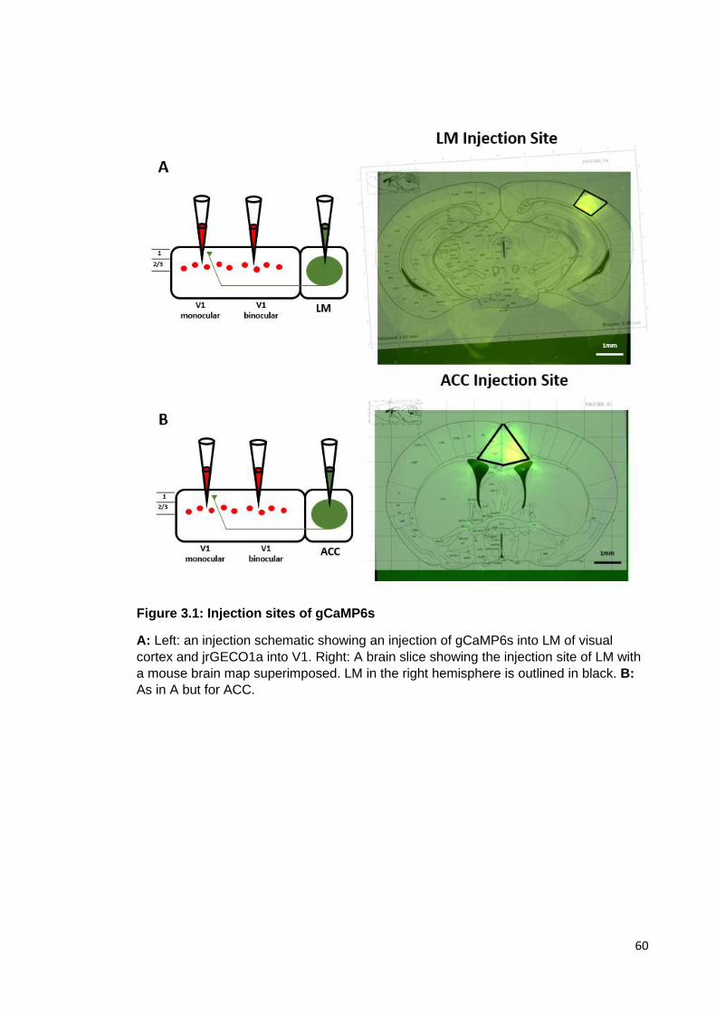
60
Figure 3.1: Injection sites of gCaMP6s
A: Left: an injection schematic showing an injection of gCaMP6s into LM of visual
cortex and jrGECO1a into V1. Right: A brain slice showing the injection site of LM with
a mouse brain map superimposed. LM in the right hemisphere is outlined in black. B:
As in A but for ACC.

61
3.2.3 Two-Photon Imaging
All in vivo calcium imaging was performed using a two-photon resonant scanning
microscope (Thorlabs, B-Scope), equipped with a Ti:sapphire laser (Coherent,
Chameleon) using a 16x 0.8 NA objective (Nikon). Awake mice were headfixed to
a custom made headplate holder and allowed to run on a spherical treadmill with
movement being measured by a rotary encoder. All imaging was carried out using
ScanImage4. Data were collected from five separate planes ranging from layer 1 to
shallow layer 2/3 of V1 in the right hemisphere, using a wavelength of 980 nm to
detect changes in fluorescence in both the jrGECO1a and gCaMP6s indicators,
while visual stimuli were presented to the contralateral eye of mouse.
3.2.4 Visual Stimulus Protocol
Visual stimuli were gratings 15° by 15° in size and appeared in 36 locations
consisting of 4 rows and 9 columns (Figure 3.2). Four orientations and eight directs
were shown consisting of 0˚, 45˚, 90˚, 135˚, 180˚, 225˚, 270˚ and 315˚. A blank was
also shown in each location. They drifted at a temporal frequency of 2 Hz and had
a spatial frequency of 0.05 cycles/deg. Each stimulus was presented for one
second and the onset of the next stimulus occurred immediately after the
termination of the previous one. Each stimulus condition was repeated 15 times.
Stimuli were presented on IIyama LED monitors positioned around the mouse with
one to the front of the mouse 10cm away and the remaining two on either side,
positioned 15cm from the mouse. Stimuli were presented from the centre of the
binocular field of view directed in front of the mouse, denoted as 0°, to 80° in the
direction of the eye contralateral to the imaged hemisphere.

62
3.2.5 Analysis
Images were initially processed using Suite2p (Pachitariu et al., 2017). This
included registering them to correct for brain motion, identifying active neuronal
somas and axons using a combination of automated detection and manual
selection and extracting calcium time courses from them described previously in
the general methods. Examples of fluorescence recorded from ACC axons and V1
somas are shown in Figures 3.3 and 3.4 respectively.
Figure 3.2: Schematic of the retinotopy protocol
Mice were presented with visual stimuli in 36 positions consisting of four rows and nine
columns. Presentation in azimuth ranged from 0˚ (in front of the mouse), and through
binocular and monocular regions of visual space of the eye ipsilateral to imaging by 80˚.

63
Figure 3.3: Example fluorescence traces extracted from ACC axons
A: Example of the fluorescence fluctuation of an ACC axon over the course of an entire
trial (top) and for a selected five minute period (bottom). B: As in A, but for a different
axon.
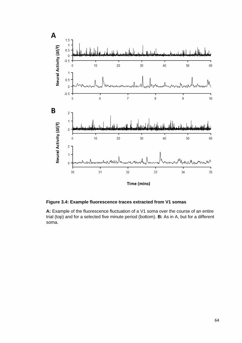
64
Figure 3.4: Example fluorescence traces extracted from V1 somas
A: Example of the fluorescence fluctuation of a V1 soma over the course of an entire
trial (top) and for a selected five minute period (bottom). B: As in A, but for a different
soma.

65
Time courses within individual experiments were then broken up on a trial-by-trial
basis. All analysis subsequent to this was carried out using custom written code in
MATLAB. For each identified soma or axon (regions of interest, ROIs), the trial with
the highest response was identified and the orientation presented within this trial
was deemed to be the preferred one. To identify ROIs which responded to a
specific location in visual space, data for each location was extracted for the
preferred orientation and then fitted with a two-dimensional Gaussian model with
the formula:
𝑓(𝑥, 𝑦) = 𝐴𝑒−(
(𝑥−𝑥𝑜)2
2𝜎𝑥2 +
(𝑦−𝑦𝑜)2
2𝜎𝑦2 )
Here, A represents the highest amplitude of response, x0 and y0 are the
coordinates of the centre of the peak and σx and σy are the spread of the peak in
the x and y directions. The fit was then manually checked to confirm the receptive
field centre (RFC) was at a peak (Figure 3.5).

66
Figure 3.5: Example of neuronal responses and the two-dimensional Gaussian fit
A: The response of each V1 pyramidal neuron that showed a location preference and then
fitted with a two-dimensional gaussian was visualised. Responses to the 36 locations were
smoothed and the star indicates the two-dimensional gaussian fit. B: As in A, but an
example of an ACC axon which exhibited a spatially specific response.

67
To identify ROIs which showed an orientation or direction preference, data for each
orientation was extracted at the preferred location. From this the orientation
selective index (OSI) could be calculated using the formula below using preferred
(pref) and orthogonal (orthog) values:
𝑂𝑟𝑖𝑒𝑛𝑡𝑎𝑡𝑖𝑜𝑛𝑝𝑟𝑒𝑓 − 𝑂𝑟𝑖𝑒𝑛𝑡𝑎𝑡𝑖𝑜𝑛𝑜𝑟𝑡ℎ𝑜𝑔
𝑂𝑟𝑖𝑒𝑛𝑡𝑎𝑡𝑖𝑜𝑛𝑝𝑟𝑒𝑓 + 𝑂𝑟𝑖𝑒𝑛𝑡𝑎𝑡𝑖𝑜𝑛𝑜𝑟𝑡ℎ𝑜𝑔
To analyse whether RFCs of axons were organised in patterns around RFCs of
somas, the mean RFC of V1 somas was subtracted from each axonal RFC
resulting in offset values in azimuth and elevation. These could then be plotted in
‘relative visual space’ encircling a centre that represented V1 somas mean RFC.
This relative visual space was then divided up into segments to investigate how
many axons were offset in each direction from the V1 somas. This was achieved
by counting the number of offset values in each segment and generating a
percentage for each segment per experiment. In the case where these groups
were further divided by orientation preferences, these counts were normalised to
the number of offset values in each segment from axons which did not show
orientation specificity. In these cases, it was important to control for a general over-
representation of offset values in particular segments. For all of these experiments,
relative visual space was limited to 30˚ in each direction to control for stimuli being
presented over a greater amount of visual space in azimuth (80˚) compared to
elevation (30˚).

68
3.3 Results
To explore the functional organisation of the top-down ACC and LM projections
into V1 compared to that of layer 2/3 V1 somas in the same location, RFC
preferences of ACC and LM axons were examined in relation to those of V1
somas. It was asked whether ACC/LM axons and V1 somas in the same area of
V1 had matching retinotopic preferences and, if not, whether there was any
consistent offset. This was then examined for ACC axons and V1 somas which
also exhibited orientation preferences to determine whether any organisation was
dependent upon orientation selectivity. To do this, the visual cortex in the right
hemisphere of mice was recorded from while drifting gratings were presented to
the contralateral eye (Figure 3.1). These gratings were 15°x15° in size and
appeared pseudo-randomly in thirty-six locations consisting of four rows and nine
columns beginning directly in front of the mouse and ranging through both
binocular and monocular fields of visual space. Four orientations were tested (0˚,
45˚, 90˚, 135˚).
3.3.1 Receptive Field Properties of ACC Axons Compared to V1 Somas
Initially, the receptive fields of ACC axons and layer 2/3 V1 somas were compared.
This study involved eight mice and 14 experimental sessions where 5087 axons
and 1622 V1 somas were identified. By considering the response profile for each
stimulus type, it was found that 8.49 ± 0.84% of ACC axons terminating in L1 V1
were visually responsive (Figure 3.6)
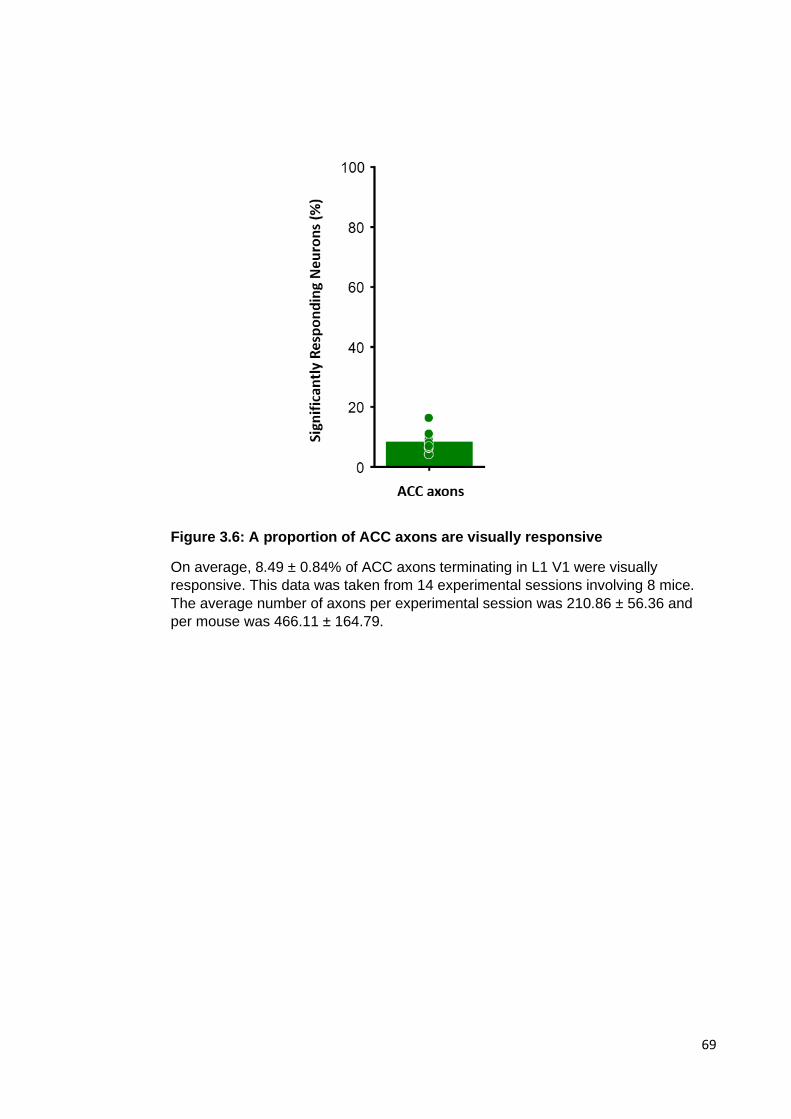
69
Figure 3.6: A proportion of ACC axons are visually responsive
On average, 8.49 ± 0.84% of ACC axons terminating in L1 V1 were visually
responsive. This data was taken from 14 experimental sessions involving 8 mice.
The average number of axons per experimental session was 210.86 ± 56.36 and
per mouse was 466.11 ± 164.79.

70
The orientation with the highest response amplitude from each identified axon and
soma was detected and, if this response was greater than that to the blank, data
were extracted from each location for this preferred orientation. A one-way ANOVA
was then carried out to find neurons that had significantly different responses
depending on location. Neurons that showed this preference were fitted with a two-
dimensional Gaussian to identify their receptive field centre (RFC), as well as
receptive field size, and manually checked to confirm the fit was at a peak. Somas
and axons which met these criteria were then taken forward in the analysis.
Both layer 2/3 V1 somas and ACC axons contained a fraction of neurons which
responded to a specific location in visual space (Figure 3.7A). An average of 18.58
± 0.95% ACC axons showed this retinotopic preference, which was significantly
less than the 52.32 ± 4.73% that observed for the V1 somas (p < 0.001, Mann
Whitney-U Test; Figure 3.7B).

71
Figure 3.7: ACC axons show retinotopic preferences
A: Examples of neural responses to each of the 36 locations in which visual stimuli were
presented. B: Although a fraction of ACC axons show retinotopic preferences, the
percentage is significantly less than V1 somas. This data was taken from 14 experimental
sessions involving 8 mice. The average number of axons per experimental session was
210.86 ± 56.36 and per mouse was 466.11 ± 164.79. The average number of somas per
experimental session were 20.42 ± 5.46 and per mouse was 130.39 ± 46.10. Standard
errors were calculated per experimental session.

72
After establishing the existence of spatial specificity in ACC axons, the size of the
scatter of RFCs were compared. RFCs for each axon and soma in four example
experiments in which somas preferred a different area of visual space suggested
that ACC axons RFCs are more scattered than those of the somas (Figure 3.8A).
To investigate this, the distance between each of the individual RFCs and the
mean RFC for the population was calculated independently for the soma and axon
neuronal populations (Figure 3.8B). ACC axon RFCs were consistently significantly
further away from their mean (p < 0.001, Mann Whitney-U Test; Figure 3.8C), and
this was true for spread in both azimuth (p < 0.005, Mann Whitney-U Test; Figure
3.4D) and elevation (p < 0.001, Mann Whitney-U Test; Figure 3.7E).

73
Figure 3.8: ACC axons carry signals from a wider area of visual space than V1 somas process in the same area of visual cortex.
A: Examples of RFCs for four experiments where V1 somas preferred different visual locations B: Schematic of the normalisation of soma and axon RFCs to their mean in order to compare RFC scatter size. The distance between each point was referred to as ∆RF, and this was then divided into Δ azimuth and Δ elevation C: The comparison between scatter sizes of RFCs in V1 somas and ACC axons D/E: As in C, but specifically for Δ in azimuth (D) and Δ in elevation (E). The average number of axons per experimental session was 49.00 ± 5.81 and per mouse was 85.75 ± 19.14. The average number of somas per experimental session were 35.86 ± 4.43 and per mouse was 62.75 ± 16.94. Standard errors were calculated per experimental session.

74
An average scatter distance greater in azimuth (20˚) than in elevation (7.5˚) could
have resulted for two reasons. The first was that ACC axon RFCs were
consistently offset by this distance from each other in azimuth and elevation
respectively. On the other hand, these values represent the average limit of spread
dictated by the size of visual space in which the visual stimuli were presented. It
was therefore possible that ACC axon RFCs were arranged randomly or in a
pattern that covered the whole of the available visual scene. To investigate this
further, the distribution of offset values in azimuth and elevation were examined by
splitting them up into bins of size 2˚ and counting how many RFCs were in each
bin (Figure 3.9). It was found that, in both azimuth and elevation, the soma RFC
count peaked at approximately the RFC mean. On the other hand, RFCs for ACC
axons were consistently spread across the visual scene in both azimuth and
elevation (Figure 3.9B/C).
Taken together, this suggested that a proportion of ACC axons responded to
specific areas of visual space, but that the relay of this information back to V1 is
not organised retinotopically. Information about a much wider area of visual space
is converging on V1 than what the somas in that area selective for.

75
Figure 3.9: The distribution of V1 soma and ACC axon RFCs across visual space in which visual stimuli were presented
A: Mean offset of RFCs of V1 somas and ACC axons from their respective mean RFCs in
azimuth and elevation. B: Frequency distribution of RFCs across visual space in which
stimuli were presented for V1 somas (red) and ACC axons (green). Each bin refers to 2˚ of
visual space. C: As in B but for elevation. The average number of axons per experimental
session was 49.00 ± 5.81 and per mouse was 85.75 ± 19.14. The average number of somas
per experimental session were 35.86 ± 4.43 and per mouse was 62.75 ± 16.94. Standard
errors were calculated per experimental session.

76
3.3.2 Receptive Field Scatter of LM Axons Compared to V1 Somas
It has been established that the somas located in the LM area of visual cortex
exhibit some classical visual response properties such as orientation and spatial
specificity (Glickfeld et al., 2013). Furthermore, axons belonging to neurons
projecting from LM and terminating in V1 show retinotopic organisation similar to
V1 (Marques et al., 2018). To further investigate the organisation of visual
properties in axons projecting from LM to V1, the same experiment and analysis
detailed above was carried out, but in this case LM axons were labelled with
GCaMP6s. This study involved five mice and six experimental sessions where 997
axons and 558 V1 somas were identified. Both layer 2/3 V1 somas and LM axons
contained a fraction of neurons which responded to a specific location in visual
space (Figure 3.10A), and the 35 ± 5.52% of axons that were retinotopically
specific was not significantly different from the 49.36 ± 9.36% of V1 somas (Figure
3.10B).

77
Figure 3.10: LM axons show retinotopic preferences
A: Examples of neural responses to each of the 36 locations in which visual stimuli
were presented. B: Although a fraction of LM axons show retinotopic preferences, the
percentage is not significantly different from that of V1 somas. This experiment
consisted of 6 experimental sessions and 5 mice. The average number of axons per
experimental session was 166.17 ± 47.87 and per mouse was 199.4 ± 66.43. The
average number of somas per experimental session were 93.00 ± 13.57 and per mouse
was 111.60 ± 27.36. Standard errors were calculated per experimental session.

78
Example experiments suggested that the mean LM RFCs mirrored the properties
of V1 somas in the area of the V1 retinotopic map into which they projected more
closely than those of ACC axons (Figure 3.11A). RFCs of each spatially specific V1
soma and LM axon were normalised to the mean soma RFCs and compared to
investigate the size of RFC scatter (Figure 3.11B). LM axons were significantly
more offset in elevation (p < 0.05, Mann Whitney-U Test; Figure 3.11D), but not in
azimuth (Figure 3.11E). Overall analysis indicates that signals carried by a subset
of LM axons are driven by spatially specific stimuli, and that these axons carry
information covering a comparable area of visual space to V1 somas in the same
retinotopic area in azimuth, but represent a larger area of visual space in elevation.

79
Figure 3.11: LM axons carry signals from a wider area of visual space in elevation than V1 somas process in the same area of visual cortex
A: Examples of RFCs for four experiments where V1 somas preferred different visual locations B: Schematic of the normalisation of soma and axon RFCs to their mean in order to compare RFC scatter size. The distance between each point was referred to as ∆RF, and this was then divided into Δ azimuth Δ elevation C: The comparison between scatter sizes of RFCs in V1 somas and LM axons D/E: Same as in C, but specifically for Δ in azimuth (D) and Δ in elevation (E). The average number of axons per experimental session was 40.67 ± 9.38 and per mouse was 48.8 ± 12.37. The average number of somas per experimental session were 30.83 ± 6.54 and per mouse was 37.00 ± 7.01. Standard errors were calculated per experimental session.

80
3.3.3 Receptive Field Offset of ACC and LM Axons from V1 Somas
ACC modulation of V1 is thought to be spatially specific (Zhang et al., 2014; Fiser
et al., 2016). An involvement in attention (Zhang et al., 2014) would suggest that
ACC axons would enhance the response of V1 neurons to relevant stimuli and so if
this stimulus is spatially specific then ACC axons need to be arranged closely to V1
neurons that respond to the same location in the visual field in order to have this
effect. LM axons projecting to V1 are believed to be involved in the processing of
moving objects, including that which occurs when the animal itself is moving
(Marques et al., 2018). In this case an offset may be expected as a prediction of
where the stimulus is likely to move to.
To explore this, the offset of ACC and LM axonal RFCs were compared with those
of the V1 somas in the same imaging region. Initially ACC axons were examined.
Imaging regions encompassed V1 somas that were responsive to stimuli across
the visual field and RFCs of ACC axons tended to the centre of the visual field
regardless of the location of the equivalent V1 soma mean RFC (Figure 3.12A).
These were then compared by normalising ACC axon RFCs to the mean soma
RFC for each experiment (Figure 3.12B), resulting in an offset value. Each offset
value represented a relative distance in visual space. To explore whether the offset
values were biased towards a particular location compared to the V1 somas, this
relative visual space was divided up into eight segments. ACC axon offset values
scattered across all eight segments (Figure 3.12C). The number of offset values in
each segment was counted and converted to a percentage for each experiment.
Offset values were limited to 30° either side of the V1 soma mean to account for a
horizontal bias arising from stimuli being presented over a wider area of visual
space in azimuth compared to elevation. It was found that there were significantly
more offset values in segments four, seven and eight than two and three (P Values

81
reported in Table 3.1; Figure 3.12D), suggesting that ACC axon RFC offset is
biased to a horizontal alignment with V1 somas.
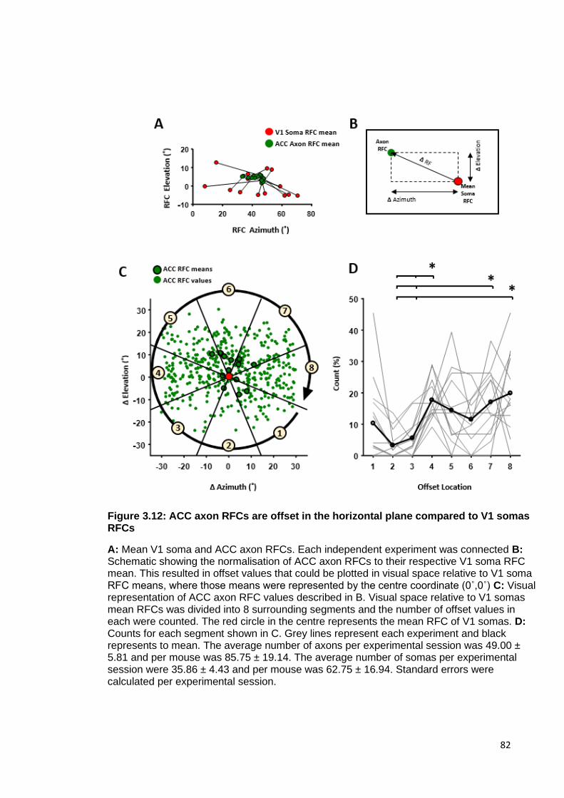
82
Figure 3.12: ACC axon RFCs are offset in the horizontal plane compared to V1 somas RFCs
A: Mean V1 soma and ACC axon RFCs. Each independent experiment was connected B: Schematic showing the normalisation of ACC axon RFCs to their respective V1 soma RFC mean. This resulted in offset values that could be plotted in visual space relative to V1 soma RFC means, where those means were represented by the centre coordinate (0˚,0˚) C: Visual representation of ACC axon RFC values described in B. Visual space relative to V1 somas mean RFCs was divided into 8 surrounding segments and the number of offset values in each were counted. The red circle in the centre represents the mean RFC of V1 somas. D: Counts for each segment shown in C. Grey lines represent each experiment and black represents to mean. The average number of axons per experimental session was 49.00 ± 5.81 and per mouse was 85.75 ± 19.14. The average number of somas per experimental session were 35.86 ± 4.43 and per mouse was 62.75 ± 16.94. Standard errors were calculated per experimental session.

83
This was then repeated for LM axons. Mean somas RFC preferences spanned
across azimuth from the monocular to binocular region of visual space. In each
case, it appeared that LM axons were offset towards binocular visual space (Figure
3.13A). To examine this further, LM axon RFCs were normalised to V1 somas in
the same imaging area as described for ACC axons (Figure 3.13B). The offset
values of LM axons were also scattered across each of the eight segments dividing
up relative visual space, but with a possible bias towards stimuli that appeared
above and towards the binocular field of view compared to V1 soma preferences
(Figure 3.13C). This was again compared using percentage counts as described
earlier, and it was found that there were significantly more axons offset in segment
8 than 1-6 (P Values reported in Table 3.2; Figure 3.13D), confirming the bias
towards the binocular direction. No significant difference between segments 8 and
7 suggested that this bias could also be directed above.

84
Figure 3.13: LM axon RFCs are offset in the binocular direction compared to V1 somas RFCs
A: Mean V1 soma and LM axon RFCs. Each independent experiment was connected B:
Schematic showing the normalisation of LM axon RFCs to their respective V1 soma RFC
mean. This resulted in offset values that could be plotted in visual space relative to V1 soma
RFC means, where those means were represented by the centre coordinate (0˚,0˚) C: Visual
representation of LM axon RFC values described in B. Visual space relative to V1 somas
mean RFCs was divided into 8 surrounding segments and the number of offset values in
each were counted. The red circle in the centre represents the mean RFC of V1 somas. D:
Counts for each segment shown in C. Grey lines represent each experiment and black
represents to mean. The average number of axons per experimental session was 49.00 ±
5.81 and per mouse was 85.75 ± 19.14. The average number of somas per experimental
session were 35.86 ± 4.43 and per mouse was 62.75 ± 16.94. Standard errors were
calculated per experimental session.

85
Segment A Segment B P Value
4 2 0.0028
4 3 0.023
7 2 0.0053
7 3 0.038
8 2 0.00029
8 3 0.0031
Table 3.1: List of p values for relative offset of ACC RFCs from their respective V1 somas
Segments refer to the area of visual space relative to V1 soma RFC means, shown in Figure 3.9C
Segment A Segment B P Value
8 1 0.026
8 2 0.00021
8 3 0.0013
8 4 0.0040
8 5 0.0092
8 6 0.00033
Table 2.2: List of p values for relative offset of LM RFCs from their respective V1 somas
Segments refer to the area of visual space relative to V1 soma RFC means, shown in Figure 3.10C

86
3.3.4 Experience-dependent properties of LM axon organisation
LM axon RFCs appeared to be biased towards binocular visual space compared to
V1 somas in the same location in V1. Studies have shown that the formation of the
retinotopic map in V1 occurs without visual experience. It is guided both by the
expression of receptors such as the EphA-ephrin-A signalling family (Cang et al.,
2005) which are arranged in a gradient across V1 (Feldheim and O’Leary, 2010),
as well as through cholinergic mechanisms that create waves of ganglion cell
discharge propagating across the retina (Wong et al., 1993) before these cells are
driven by rods and cones. It is not known, however, whether this would be
sufficient to allow the retinotopic organisation of LM inputs into V1 without visual
experience. Therefore, to understand this, the study was repeated in mice that had
been dark reared. This consisted of placing animals into the dark before eye
opening and then recording from LM axons in layer 1 V1 as well as layer 2/3 V1
pyramidal neuron somas as described earlier in this chapter. Dark reared mice
were imaged over three sessions, once immediately after removal from the dark,
then at 7 and 28 days after this (Figure 3.14A). Light reared control animals were
imaged at session one. The imaging protocol was the same as previously
described and consisted of presenting visual gratings in 36 locations using 4
orientations and 8 directions (Figure 3.14B). The light reared control group
consisted of five mice, six experimental sessions, 997 identified LM axons and 558
identified V1 somas. Session one, two and three after dark rearing consisted of six,
seven and six mice, six, seven and seven experimental sessions, 2591, 2999 and
4744 identified axons and 615, 813 and 837 identified somas respectively.
It appeared as though visual responsiveness of V1 neurons and LM axons was
reduced when mice were dark reared compared to light reared controls, but this did
not reach significance (Figure 3.14C).

87
Figure 3.14: Dark reared experiment
A: Schematic of the dark rearing experiment B: Schematic of the experimental set-up.
Mice were shown visual stimuli as described previously C: The percentage of V1 somas
and LM axons which exhibited spatially specific activity. Light reared data is from the
same cohort as used previously. The light reared control involved 6 experimental
sessions and 5 mice. Dark reared session 1 involved 6 experimental sessions and 6 mice;
dark reared session 2 involved 7 experimental sessions and 7 mice and dark reared
session 3 involved 7 experimental sessions and 7 mice. The number of axons or somas
per experimental session and per mouse are shown in Table 3.3

88
Session Exp No Mouse No Mean ROI per
exp/mouse
1 6 6 431.83 ± 203.79
2 7 7 165.57 ± 53.65
3 7 7 525.71 ± 208.55
1 6 6 102.50 ± 7.86
2 7 7 104.57 ± 8.32
3 7 7 109.00 ± 5.98
Table 3.3: The number of experimental sessions and mice used for each dark reared session.
Sessions refer to dark rearing session with session one being immediately after
removal from the dark, session two one week after this and session three four weeks
after session two. The exp no refers to the number of experimental sessions for each
experiment. The mouse number refers to how many mice were used for each dark
rearing session. The mean ROI per experiment or mouse is the same in this case as
only one area was imaged per mouse. Green highlighted rows indicate information for
LM axons and red highlighted rows indicate information for V1 somas.

89
After this, RFC scatter was then examined for V1 somas and LM axons in dark
reared animals and compared to those of light reared controls. Example
experiments for each of the three imaging sessions taken from one animal
indicated that LM axon RFCs of dark reared animals are scattered across visual
space (Figure 3.15A-C). In these experiments the axons were not specifically
tracked, but the imaged area was the same and so there was likely to be overlap in
axon populations across imaging sessions. LM axon and V1 soma RFCs were then
normalised to their respective means to examine the scatter of the receptive fields.
There was no significant difference between the scatters for the overall change in
receptive field (Figure 3.16A-C). It could be noted, however, that dark reared axon
means are clustered around 20˚ for a change in azimuth (Figure 3.16B) and 7.5˚
(Figure 3.16C) for change in elevation, reminiscent of ACC axon arrangement
which was shown to feed information from across visual space to V1 somas.
To examine further whether LM axons of dark reared mice projecting to V1 showed
a bias to RFC locations towards the binocular area of visual space, LM RFCs were
normalised to their equivalent V1 soma RFC as described previously. For each
session after dark rearing, LM axon RFCs tended towards the centre of visual
space in which stimuli were presented, suggesting the binocular bias was not
apparent (Figure 3.17A-C). After normalisation, relative visual space was again
divided into 8 segments and offset values were analysed as previously described
(Figure 3.18A/C). As session one only had mean soma RFCs covering one half of
the visual space in which stimuli were presented, it was discounted from this
analysis. In session two, it was found that there was no significant difference
between the number of offset values in any of the segments (Figure 3.18B). In
session three, there were significantly more offset values in segment 4 than
segments 2 and 3 (P values reported in Table 3.3; Figure 3.18D). This suggested

90
that not only was there no bias towards the binocular area of visual space, but that
the bias which did emerge was in the opposite direction. Taken together, these
data suggest that visual experience is required for the development LM axonal
functional organisation in V1 observed in light reared mice.
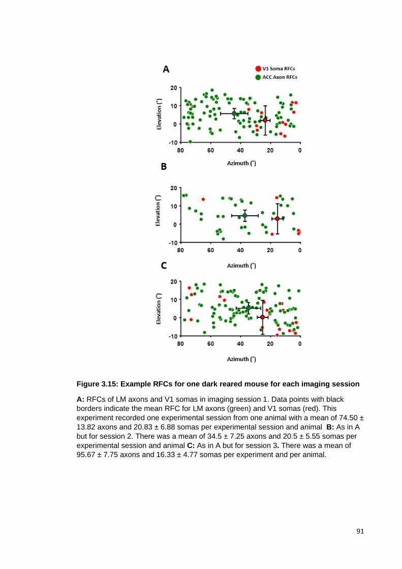
91
Figure 3.15: Example RFCs for one dark reared mouse for each imaging session
A: RFCs of LM axons and V1 somas in imaging session 1. Data points with black
borders indicate the mean RFC for LM axons (green) and V1 somas (red). This
experiment recorded one experimental session from one animal with a mean of 74.50 ±
13.82 axons and 20.83 ± 6.88 somas per experimental session and animal B: As in A
but for session 2. There was a mean of 34.5 ± 7.25 axons and 20.5 ± 5.55 somas per
experimental session and animal C: As in A but for session 3. There was a mean of
95.67 ± 7.75 axons and 16.33 ± 4.77 somas per experiment and per animal.

92
Figure 3.16: Scatter of LM axons and V1 soma RFCs after dark rearing
A: The scatter of V1 somas and LM axon RFCs for the light reared control (left), and for
each of the imaging sessions after dark rearing for ΔRF. Each data point indicates the mean
for an experimental session B: As in A but for Δ Azimuth. C: As in A but for Δ Elevation.
Light reared data is from the same cohort as used previously. The number of axons and
somas per experiment and per mouse were described in Figure 3.14

93
Figure 3.17: Mean V1 soma and LM axon RFCs for dark reared mice
A: RFCs from imaging session 1. Each independent experiment is connected. B: As in A,
but for imaging session 2. C: As in A but for imaging session 3. The number of axons and
somas per experiment and per animal were as described in Figure 3.14.

94
Figure 3.18: LM axon RFC offset from V1 soma mean RFCs is not in the direction of the binocular zone after dark rearing
A: Visual representation of LM axon RFC offset values as described in figures 3.9C and
3.10C but for the second session after mice were dark reared. B: Counts for each segment.
Grey lines represent each experiment and black represents to mean. C/D: As in A/B
respectively but for session 3 after dark rearing. Numbers of mice, experimental sessions
and average number of axons and somas identified are given in Table 4.

95
Segment A Segment B P Value
4 2 0.0067
4 3 0.0035
Table 3: List of p values for relative offset of LM RFCs from their respective V1 somas for dark reared mice
Segments refer to the area of visual space relative to V1 soma RFC means, shown in Figure 3.15C. P values reported here are for session 3.
96
3.3.5 Functional organisation of ACC RFCs compared to V1 somas RFCs is not
dependent on orientation selectivity
ACC axons appear to have RFCs biased somewhat to the horizontal axis of visual
space relative to RFCs of V1 somas in the same imaging area. It remains
unknown, however, whether there is any functional organisation of ACC axons
dependent on orientation selectivity. It has been shown previously that LM axons
projecting to V1 respond preferentially to areas of visual space located
orthogonally from their orientation of preference (Marques et al., 2018). It might be
the case that the spatial functional organisation of ACC axons is dependent on
orientation preferences of axons.
First, orientation preference was explored in V1 somas and ACC axons in the
same location within V1. To examine this, the Orientation Selectivity Index was
calculated for each neuron (see methods). A significantly higher percentage of V1
somas, at 33.67 ± 2.44 preferred 90˚ to other orientations with 25.00 ± 2.12%,
17.33 ± 2.26% and 24.00 ± 1.26 preferring 0˚, 45˚ and 135˚ respectively. This was
in line with V1 somas preferring cardinal rather than oblique orientations. (Xu et al.,
2006; Drager 1975) (Figure 3.19A). Proportions of ACC axons also showed
orientation selectivity, although the number of neurons that responded to each
orientation were comparable at 25.71 ± 1.89%, 23.21 ± 1.35%, 25.09 ± 1.48% and
26.00 ± 1.91% responding to 0˚, 45˚, 90˚ and 135˚ respectively (Figure 3.19B).

97
Figure 3.19: ACC axons show orientation selectivity but there is not an over-representation of cardinal orientation preference
A: The percentage of V1 somas, out of all those that exhibited orientation preferences, that preferred each of the four orientations presented (left). Examples of somas which preferred each orientation (right). B: As in A but for ACC axons. This involved a mean of 51.64 ± 8.84 axons and 24.21 ± 2.51 somas per experimental session.

98
After establishing that some ACC axons exhibited orientation preferences, it was
investigated whether there was any organisational pattern of RFCs dependent on
orientation specificity. To explore this, ACC axons and V1 somas that showed both
spatial and orientation preferences were considered. This included 61, 54, 71 and
70 ACC axons that preferred 0°, 45°, 90° and 135° oriented stimuli respectively.
Initially, axon RFCs were normalised to the mean soma RFC of the V1 somas in
the same imaging area to calculate a change in RF (Figure 3.21A) resulting in
offset values as described previously. These offset values were also calculated for
axons that were spatially specific but did not exhibit an orientation preference
(Figure 3.21B) for later normalisation of the percentage counts. The relative visual
space around the mean soma RFC was then split into four segments (Figure
3.21C) in which the offset axonal RFCs could lie. The RFC pattern of each
orientation was taken into account individually and so there were three populations
of axonal RFC within each segment – those of the current orientation, those of the
other three orientations, and those that only show spatial specificity (Figure 3.21D).
The organisation of ACC axon RFC offset values was explored for each orientation
independently and the positioning of each segment in visual space depended upon
the orientation under investigation. The parallel segment would always be the area
of relative visual space along the long axis of the orientation in question, and the
perpendicular would be along the short axis (Figure 4.21E). RFCs for each
orientation in each segment were counted within a radius of 30˚ and normalised to
the number of RFCs in that segment that did not show an orientation preference.
This was to control for stimuli being presented over a larger degree of visual space
in azimuth. For each orientation within each experiment, a percentage was
calculated for how many offset values were in each relative segment compared to
the other three. These values were then compared using an n-way ANOVA. There
was no significant different between the number of RFCs in each of the relative
segments for any of the four orientations tested. This suggested that there was no

99
organisation of ACC axon RFCs dependent on orientation preference (Figure
3.21B).

100
Figure 3.20: Orientation-dependent organisation of ACC axon RFC offset from V1 somas
A: Schematic showing the calculation of ACC axon RFC offset values for axons which responded
to both a specific location and orientation of visual stimulus. B: As in A but for axons that did not
show an orientation preference C: The relative visual scene where the centre coordinate
represented V1 soma RFC means was divided into four segments D: Each of the different groups
of ACC axon that were present in each segment. E: The relative arrangement of each of the
segments of visual space relative to V1 soma RFC means. Segments were arranged depending
on the orientation under investigation. Parallel segments were always arranged along the long
plane of the orientation, and perpendicular segments were always orthogonal. For example, for
axons that preferred 0˚ (left diagram), the parallel segment was on the horizontal plane, and for
axons that preferred 90˚, the parallel segment was on the vertical plane.

101
Figure 3.21: Organisation of ACC axon offset values relative to their orientation preferences
A: An example of the distribution of ACC axon offset values for ACC axons preferring visual
stimuli of orientation 135˚. Green dots indicate the relative offset of ACC axon RFCs from the
mean of the V1 soma RFC, indicated by the red dot in the centre. B: There was no
preferences for any area of visual space depending on orientation preference. This involved a
mean of 51.64 ± 8.84 axons and 24.21 ± 2.51 somas per experimental session.

102
3.4 Summary of Findings
1. A fraction of ACC axons have spatially selective responses, but the proportion
showing these was significantly lower than for V1 somas.
2. A fraction of LM axons have spatially selective responses, and the proportion
showing these was comparable to that for V1 somas.
3. ACC axon RFCs were significantly more scattered in both azimuth and
elevation compared to V1 soma RFC scatter.
4. LM axon RFCs were significantly more scattered only in elevation compared to
V1 somas.
5. ACC axon RFCs were offset towards the horizontal plane compared to V1 soma
RFCs.
6. LM axon RFCs were offset towards the binocular field of view, and this appears
to be dependent on visual experience.

103
4 The Involvement of Anterior Cingulate Cortex Axons
Terminating in Primary Visual Cortex in Visually Guided
Tasks
4.1 Introduction
The sensory environment has a plethora of stimuli which the brain is unable to process
at once. To successfully navigate this world, the brain must be able to focus attention
amongst competing stimuli onto those which are important (Desimone and Duncan,
1995) and coordinate relevant responses. This is apparent, for example, when
searching for food or when evading predators. To achieve this, two processing streams
are used, known as bottom-up and top-down projections. In the visual system, bottom-
up projections faithfully relay information about particular visual stimuli such as their
location and orientation. They are most crucial in directing attention in unfamiliar
scenarios to visual features of potential importance such as the movement of a
predator or a car. As scenarios gain familiarity, bottom-up projections are believed to
dynamically interact with top-down influences (Makino and Komiyama, 2015) that use
previous experience to guide attention to specific stimuli. These are believed to be
internal projections originating primarily from the frontal (Miller and Cohen, 2001) and
parietal regions (Kastner and Ungerleider, 2000; Bisley and Goldberg, 2010), such as
the frontal eye field (Zhou and Desimone, 2011; Squire et al., 2013), and have been
implicated not only in the direction of attention (Zhang et al., 2014), but also in the
development of spatial maps (Fiser et al., 2016) as well as influencing processing
during motion (Niell and Stryker, 2010; Keller et al., 2012; Bennett et al., 2013; Saleem
et al., 2013; Erisken et al., 2014).
Where various stimuli are competing for finite processing resources, learning to direct
attention towards stimuli that are behaviourally relevant and can be associated with a
reward or avoiding an aversive stimulus will be favoured. Using previous experience to

104
focus attention upon a stimulus that holds behavioural relevance appears to involve a
strengthening of top-down activity coupled with the weakening of bottom-up signals,
something that has been implicated during learning (Makino and Komiyama, 2015) and
perceptual memory consolidation (Miyamoto et al., 2016). This would require an
integrated system able to identify the visual stimulus, make a decision based upon it,
process the consequences of that decision and use that information to inform
subsequent choices based on what has been learned.
It has been extensively reported that neurons in V1 respond more to visual stimuli that
are being attended to compared to those which are not (Moran and Desimone, 1985;
Corbetta et al., 1991; Treue and Maunsell, 1996) and that paying attention to a
stimulus that is behaviourally relevant in particular works to strengthen the
corresponding neuronal representation (Poort et al., 2015; Daliri, Kozyrev and Treue,
2016; Keller et al., 2017). Attending to specific stimuli in the environment requires a
decision to be made and this will be influenced by association of a stimulus with a
rewarding or aversive outcome. Therefore, processing of reward and subsequent
decision making are essential in deciding where to direct attention. The anterior
cingulate cortex (ACC) has been strongly implicated in decision making, especially
when influenced by reward. Rats with lesions at the ACC tend to always choose a
lower reward when greater effort is needed to obtain a larger reward, whereas rats with
an intact ACC go for the higher reward (Schweimer and Hauber, 2005) suggesting an
importance in choosing the appropriate option when responses have competing
outcomes (Cocker et al., 2016). Located within the prefrontal cortex, a structure
implicated in goal-directed activity (Miller and Cohen, 2001), the ACC is also the source
of many long-range top-down projections. In the mouse, it projects extensively to
multiple sensory cortices including the auditory cortex, somatosensory cortex and
visual cortex (Zhang et al., 2016). This suggests that an interaction between ACC and
105
V1 is a prime candidate for controlling visual attention in tasks that involve detecting
and subsequently making a decision based on a stimulus in order to obtain a reward.
One such projection originating at ACC and terminating predominantly in layer 1 of V1
has been identified (Zhang et al., 2014). Recent studies have, however, highlighted
discrepancies in its believed functionality. One idea is that this circuit is involved in
aiding visual attention. Optogenetic activation of this projection not only sharpened
orientation tuning of neurons in V1, but also improved performance in a visual
discrimination behavioural task suggesting an involvement in selective attention as well
as exhibiting spatially specific responses. This projection is believed to act through
local inhibitory circuits with somatostatin positive GABAergic interneurons contributing
preferentially to surround suppression and vasoactive intestinal peptide-positive
interneurons critical for centre facilitation (Zhang et al., 2014). Other evidence, from
another recent study, has suggested it instead has a key role in developing an internal
representation of the visual environment based on spatial location. In this study, head-
fixed mice were allowed to explore a virtual tunnel where the presentation of four
stimuli in a specific order was coupled to the movement of the mouse on a rotating
spherical treadmill. Under these conditions initially axons projecting from ACC were
only responsive to the visual stimuli when on the screen but as the mouse was
exposed to more trials, these responses occurred just before the stimuli appeared. This
suggests that temporal tuning of activation of the projection becomes predictive as a
visual stimulus gains spatial relevance while mice learn to navigate an environment
(Fiser et al., 2016).
Following on from the work of Zhang et al. (2014), I asked the question of whether the
ACC→V1 top-down circuit is endogenously recruited to improve performance in a
visually guided discrimination task. To address this question, two-photon microscopy
was used to image axons originating from ACC in layer I of V1 while animals performed

106
the same go/no-go visual discrimination task employed by Zhang et al (2014). It was
hypothesised that, once mice learned the task and exhibited high performance, ACC
activity would be apparent, and specifically elevated during correct trials. Furthermore,
as ACC activity would be influenced by the retinotopic location of the visual stimulus
presented.

107
4.2 Materials and Methods
4.2.1 Mice
All procedures performed on animals were carried out in accordance with institutional
and UK welfare guidelines as previously stated. Mice were kept in standard laboratory
conditions which involved cycles of 14 hours of light and 10 hours of darkness at 24°C.
They were provided with a standard diet and water ad libitum unless on water
restriction. Water restriction was implemented during the course of the behavioural
tasks, beginning approximately three days before studies commenced. A daily
allowance of water was calculated for each mouse individually based on weight. Mice
were able to obtain this during the behavioural task each day, and if they did not reach
the allowance limit then the rest was given directly after. The weight of each mouse
was monitored daily to ensure it did not drop below 80% of the original baseline weight
of the mouse. Experiments involved both wildtype (WT) mice and those in which
parvalbumin positive (PV+) interneurons were labelled with the red marker tdTomato,
achieved by crossing B6.Cg-Gt(ROSA)26Sortm14(CAG-tdTomato)Hom/J and B6;129-
Pvalbtm1(cre)Arbr/J (Jackson Laboratory, JAX Stock 007914 and 008069,
respectively). Wildtype mice were ordered from Charles River and PV-CRE mice were
bred in-house. All mice were housed with same sex littermates and were provided with
running wheels.
4.2.2 Viral Injection and Cranial Window Implant
Experiments involved mice where just ACC axons were labelled with a calcium-
sensitive indicator, as well as mice where both ACC axons and layer 2/3 V1 somas
were labelled. To achieve this, methods previously described in the general methods
and previous result chapter were used. Mice used in the detection task were injected
with a type of gCaMP6s that was preferentially transported to axons (Broussard et al.,
2018).

108
4.2.3 Intrinsic Signal Imaging
Intrinsic signal imaging was used to identify the area in monocular V1 to image from.
This was achieved using methods previously described in the general methods.
4.2.4 Visual Discrimination Task
Mice were placed on water restriction and behavioural training commenced after they
reached 80% of their initial weight. They were headfixed and the custom-designed
fixed axis treadmill was locked to prevent locomotion. Behavioural training for the
go/no-go visual discrimination task consisted of three stages, including stage one, two
and the testing stage. Each stage was controlled by custom-written code in MATLAB
that automatically progressed the mice to the next stage after reaching a pre-defined
threshold. On correct go trials mice were rewarded with KoolAid® (Craft Foods).
Stage one (Figure 4.1) consisted of building an association between licking the reward
spout and obtaining a reward. At this point, no visual stimuli were presented to the
mice. Each trial could last up to 60s, but if the mouse licked the spout then it was
immediately given a reward and moved into a variable quiescent period (Figure 4.1B).
During the quiescent period of the task, a lick of the spout would not result in a reward.
This was to reinforce that rewards could not be obtained at all times. The quiescent
period was temporally variable so that mice could not predict when to lick the spout to
obtain a reward based on time. This was important for later stages where mice were
required to lick the spout at certain times and withhold at others. Mice were able to
consistently lick the spout throughout the session, as well as complete trials with a
minimum of a two second quiescent period prior (Figure 4.1C/D). Once mice were
consistently licking the spout with a median response time of less than 5s over a period
of 20 trials, they were progressed to stage two.

109
Figure 4.1: Stage one of the visual discrimination task
A: Schematic of stage one of the task. This stage was used to associate licking the
spout with gaining a reward. As in later stages of the task the reward would only be
given under certain circumstances, a reward was not given for every lick. Instead, if
the animal licked within the trial then it would immediately receive the reward and be
shifted into the quiescent period. Licking during this quiescent period did not result in a
reward, and mice had to refrain from licking for at least two second before beginning
the next trial. This was important to reduce continuous repetitive licking. No visual
stimuli were shown at this stage B: Diagram of stage one of the task. The top arrow
shows that after the mice lick at any point during the trial, they are immediately shifted
into the quiescent period. The lower arrow indicates that after the quiescent period,
mice are shifted to the next trial as described in A. C: Mice lick consistently throughout
the course of this stage D: Lick raster plot shows that mice do not continuously lick the
spout. The grey section indicates the quiescent period.

110
Stage two (Figure 4.2) consisted of introducing the go stimulus and pairing it with the
lick response to obtain a reward. An auditory tone occurred 0.5s prior to the onset of
the trial. The visual stimulus was then presented to the mouse for a period of four
seconds (Figure 4.2A/B). The response of the mouse was disregarded during the first
two seconds of stimulus presentation as mice were likely to exhibit impulsive licking
when the visual stimulus appeared and contributed to the outcome of the trial in the
latter two seconds of presentation, referred to as the response window. The go
stimulus was paired with the reward by having a mix of ‘free reward’ and ‘normal’ trials.
In the ‘free reward’ trials, the reward would be given at 3.5s if the animal did not lick the
spout during the response window and the trial was classed as incorrect. If the mouse
licked the spout in the response window prior to 3.5s then it immediately obtained the
reward and this was classed as a correct trial. In ‘normal’ trials, a correct trial was
recorded if the mouse licked and obtained a reward in the response window. If the
animal did not lick the spout throughout the response window then it would not receive
the KoolAid® and the trial was deemed incorrect. Stage 2 began with 90% ‘free reward’
trials and 10% ‘normal’ trials. These proportions changed by 10% if the mouse
achieved a performance of 70% correct until 100% of trials were ‘normal’ (Figure 4.2C).
Mice improved in performance across this stage (Figure 4.2D) and once their
performance at 0% ‘free reward’ trials reached 70%, they were progressed to the
testing stage of the task.

111
Figure 4.2: Stage two of the visual discrimination task
A: Schematic of stage two of the task. This stage was used to associate licking the spout in
response to the presentation of the go stimulus with a reward. B: Diagram of the visual
discrimination task. C: Diagram of the progression through stage 2 where mice are given a
changing proportion of ‘free’ and ‘normal’ trials. This begins at 100% ‘free’ trials and 0%
‘normal’ trials. Mice progress if they complete over 70% of trials correctly in 10% percentage
intervals to 100% ‘normal’ trials and 0% ‘free’ trials, and then subsequently onto stage three.
D: An example experiment indicating that mice increase in performance (calculated by
percentage correct) over the course of stage two and reach the 70% threshold.

112
The testing stage introduced the no-go stimulus, a grating of orientation 0˚ which drifted
upwards. If the mouse licked the spout during the response window of a no-go trial
then it received an air puff, white noise and a ten second time-out. This encouraged
licking the spout only in response to the go stimulus. Performance was calculated use
d’ (d’ = ZFA - ZHit). High performance was considered to be a d’ of greater than 1.5
and a HR-FA rate of greater than 0.5.
Two forms of the visual discrimination task were used. The first involved the go and no-
go visual stimuli being presented in the same spatial location in each trial, and to the
contralateral eye to imaging. This version was referred to as the retinotopically
predictable format. The second design comprised the visual stimuli being presented in
the monocular field of either the contralateral or ipsilateral eye in a pseudorandom way,
and thus the mice were not able to predict exactly where the stimulus would appear.
This was referred to as the retinotopically unpredictable format. This allowed the
investigation into whether ACC activity was retinotopically specific, as well as
examining ACC activity in an arguably more difficult visual discrimination task.

113
4.2.5 Visual Detection Task
Studies have shown that the ACC projection to V1 is retinotopic and may exhibit
properties similar to surround suppression (Zhang et al., 2014), something that is
characteristic of top-down modulation. It was therefore possible that ACC activity
properties would be overlooked in the visual discrimination task due to the large
stimulus required. To address this in this study, a visual detection task was developed
which allowed for a smaller stimulus. Mice that had both ACC axons and layer 2/3 V1
somas labelled were used in this experiment so that it was possible to image locations
in V1 that were retinotopically matched to the stimulus, and then move the stimulus
outside of this area. Mice were placed on water restriction and behavioural training
commenced after they reached 80% of their initial weight. Behavioural training for the
detection task was based on the same three stages already described in the visual
discrimination behaviour. Stage one was identical with the same aim of associating
licking the spout with gaining a liquid reward of KoolAid®. Stage two introduced the go
stimulus, but the response window lasted the entire length of the presentation rather
than just the second half. Mice again progressed through trials where there were a high
proportion of ‘Free Rewards’ relative to ‘Normal’ trials, which reversed as performance
improved and entered a variable quiescent stage in between trials. The testing stage
consisted of a go/no-go structure where a blank was shown in the no-go trials, but the
incorrect response of licking during this time did not result in an air-puff, white noise or
time-out. This design made it possible to investigate ACC axonal responses to a visual
stimulus both inside and outside of the matched receptive field of the layer 2/3 V1
somas directly ventral in the cortex. Furthermore, it was possible to begin to separate
axon activity levels at the visual stimulus onset and when the mouse licked the spout to
gain a reward due to reaction time causing a slight temporal delay between the two.

114
4.2.6 Perfusion and Histology
Mice were given a lethal intraperitoneal injection of sodium pentobarbital (Euthatal;
Merial Animal Health). After there was no response to tail pinch and the mouse had
stopped breathing, it was perfused. This consisted of opening the chest cavity to
expose the heart. A needle attached to a pump was inserted into the left ventricle and
the right atrium was snipped. This allowed 0.1M phosphate-buffered saline (PBS) to be
fed through the circulatory system in order to remove the blood. Once the blood had
been cleared, 4% paraformaldehyde (PFA) in PBS was pumped through to fix the
tissue. The brain was then dissected out and submerged in PFA for another four hours.
Each mouse brain was sliced at 80 µm using a vibratome. Slices were mounted onto
gelatin-covered microscope slides, left to adhere and dry, re-hydrated and then
coverslipped using Fluoromount Aqueous Mounting Medium. Mounted slices were
imaged using a confocal microscope.
4.2.7 Data Analysis of Neuronal Activity
Analysis was carried out using Python and MATLAB. Images were extracted and
registered using Suite2p (Pachitariu et al., 2017). To analyse neural activity on a trial-
by-trial basis, fluorescence timecourses of gCaMP6s or jrGECO1a representing ACC
axon and V1 soma activity within individual experiments were broken up by aligning to
an element of the behaviour, for example the onset of the visual stimulus or the timing
of the rewarded lick. Neurons were considered to be responsive to a particular stimulus
if there was a significant change in activity compared to a baseline time calculated for
each trial independently across an experimental session using a repeated measures
ANOVA test. In some cases, this was done for a specific time window within the trial
such as the visual stimulus onset or response window of the visual discrimination task.
In other cases, significantly increased responses were examined at 0.2s time intervals

115
after the defined baseline time before the start of the trial. This was to identify when
axons or somas began to respond during the tasks, and to make sure responses were
not discounted because the occurred prior to a specific relevant time window,
something that may occur otherwise if predictive or preparatory responses were
exhibited.
Where data was not extracted as trials, correlational analysis and permutation tests
were used. This involved comparing fluorescence data to lick frequency and
locomotion data. Lick data was collected at 1000 Hz in binomial form. It was converted
to rate over a time kernel of 1s and then resampled to 5 Hz to match the fluorescence
data timings. A permutation test was then carried out by correlating the resulting lick
data with the fluorescence trace, before incrementally shifting the fluorescence trace
circularly and calculating a correlation coefficient for each shift. The 100 coefficient
values for each individual session were ranked, and if the original value was in the top
fifth percentile then calcium activity was considered to be significantly associated with
lick frequency. The same method was used to examine the association of locomotion
and neural activity, although in this case wheel velocity (i.e. running speed of the
animal) was used in place of lick frequency. Values are given as mean ± SEM unless
otherwise stated.

116
4.3 Results
4.3.1 Learning a retinotopically predictable go/no-go visual discrimination task
Mice are able to learn a range of visually guided tasks when head-fixed, including
those where different stimuli are passively presented, as well as those using virtual
reality corridors linked to the movement of the mouse (Chen et al., 2013; Poort et al.,
2015). In this study, the endogenous activity of ACC axons was explored while animals
performed a go/no-go visual discrimination task while stationary to investigate whether
ACC axons exhibited elevated activity at specific time windows within the task; as well
as whether ACC axon activity was generally elevated when the task was being
performed successfully. The go/no-go visual discrimination task was implemented
based on that used in Zhang et al., (2014) and Andermann et al., (2010). Head-fixed
animals were trained to discriminate between the go stimulus, a vertical grating drifting
forwards, or the no-go stimulus, a horizontal grating drifting upwards, by licking a spout
to receive a liquid reward in response to the go stimulus. Animals were positioned on a
spherical treadmill which was locked in place to prevent locomotion. Each stimulus was
presented for four seconds and the lick response of the mouse was recorded in the
final two seconds, known as the response window. High performance on this task was
achieved by training animals through three stages (see methods).
During the testing stage, trials consisted of presenting the mouse with either the go or
the no-go stimulus in a retinotopically predictable location in the monocular region of
the contralateral eye (Figure 4.3A). Each trial (Figure 4.3B) was preceded by an
auditory tone sounded 0.5s before the onset of the visual stimulus. The go or no-go
stimulus would drift for four seconds, and the lick response of the animal would only
lead to correctly or incorrectly completing the trial in the latter two seconds to reduce
the impact of impulsive licking. Licking the spout was only reinforced during the go
trials, and if the mouse licked the spout during the response window of the no-go trial it

117
received an air puff, white noise and a 10s time-out. Performance was quantified by
calculating d’ (see methods) which measured the difference in proportions of hit and
false alarm trials. A higher d’ indicated a higher level of performance. The following
study included six mice, 16 experimental sessions and 2007 identified axons.
Over the course of training, the lick responses of the mice aligned to specific elements
of the task including the sounding of the tone and the response window of go trials, the
latter being indicative of an improvement in performance. (Figure 4.3C). On average,
mice were able to achieve a high level of performance (defined as d’ > 1.5) after 8 days
of training during this stage (Figure 4.3D); and were generally able to perform this
behaviour consistently over days with only rare drops in performance (Figure 4.3E).
The performance of each animal was considered independently.

118
Figure 4.3: Mice can perform a go/no-go visual discrimination task
A: Schematic of the retinotopically predictable discrimination task. B: Diagram of the visual
discrimination task. C: Lick raster plots: top – early training session before the mouse has
learned the task; bottom – training session where the mouse exhibits high performance. D:
Mean performance of all mice. Lines indicate the best fit (blue) and the high performance
threshold (red) E: Example performance of an individual mouse. The red line shows the high
performance threshold.

119
4.3.2 The activity of ACC axons was elevated during specific time windows
during the go/no-go discrimination
To label ACC axons projecting to V1, GCaMP6s was injected into ACC (Figure 4.4A).
This injection site is shown in Figure 4.4B. After approximately four weeks GCaMP6s
filled axon terminals could be visualised both at the site of injection at ACC and
throughout the depth of V1, with the highest density in layer 1 (Figure 4.4C). A cranial
window was implanted above V1 of the right hemisphere and intrinsic signal imaging
was used to localise V1 (see general methods) before using two-photon microscopy to
functionally measure activity of the axons.

120
Figure 4.4: ACC injection and cranial window implant
A: Top: Approximate position of ACC and V1; bottom – ACC injection schematic. B:
Histology of ACC injection. Top - injection site at ACC where GCaMP6s transfected
neurons appear green/yellow. This image is superimposed by a schematic of the
mouse brain atlas (also shown below the image) to confirm the injection was made in
ACC. C: visual cortex where the green colour in layer I indicates axons labelling.

121
Initially the question of whether ACC axon activity increased during the task as the
mice learned was addressed. To do this, ACC axonal responses from the first session
in which the mouse was exposed to either the go or no-go stimulus were compared
with when the mouse exhibited high performance on the task. Axons were not
specifically tracked but were sampled from the same location in V1 and so were likely
to be made up of a similar population. A percentage of 39.16 ± 3.54% of ACC axons
responded during the presentation of the go stimulus once the task had been learned,
significantly higher than the 18.29 ± 5.26% that responded the first time the go stimulus
was shown to the mice. No significant difference was observed during no-go trials with
23.62 ± 8.52% responding the first time the no-go stimulus was shown and 31.65 ±
4.22% responding when performance was high (Figure 4.5A/B).
After this, the responsiveness of 2007 axons was measured during behavioural
sessions where the mice exhibited high performance. Axons were divided into go and
no-go conditions before sorting trials by the time of peak activation. It was observed
that subsets of axons were active at time points spanning the entire trial in both
conditions (Figure 4.5C). Although axons were observed to respond exclusively to
either go or no-go trial types, it was clear that overall activity levels were significantly
higher during go trials as compared to no-go trials with 29.68 ± 3.04% and 11.52 ±
1.20% of axons showing activity over the entire trial respectively (p < 0.001, one-way
ANOVA). It was also noted that 6.33 ± 1.80% of axons responded indiscriminately to
both types of trial, which was significantly less than those exclusively responding to go
trials (p < 0.001, one-way ANOVA), but comparable to those responding to no-go trials
(Figure 4.5D).
Each trial was made up of two main elements, namely the presentation of the visual
stimulus and the response window, and further investigation was carried out to find out

122
which of these the axons were active in. When the visual stimulus was presented,
24.29 ± 3.18% of axons responded exclusively to the go stimulus which was
significantly more than the 8.15 ± 1.87% to the no-go stimulus (p < 0.001, one-way
ANOVA). This was also significantly more than the 5.79 ± 1.19% that responded to
both stimuli (p < 0.001, one-way ANOVA). Additionally, significantly more axons were
active during the response phase of task during go trials with 26.56 ± 3.68% compared
to 10.57 ± 1.64% in the no-go trial (p < 0.001, one-way ANOVA). Furthermore,
significantly more axons were active exclusively in either the go (p < 0.001, one-way
ANOVA) or the no-go (p < 0.05, one-way ANOVA) trials during this phase of the trial
compared to indiscriminately active axons (Figure 4.5D).
This analysis indicated that axons were active during each phase of the task when it
was performed correctly, but that there were a significantly higher percentage of axons
that responded to the go stimulus in comparison to the no-go stimulus. Additionally,
when the mice were required to make a response, significantly more axons responded
exclusively to either the go or no-go stimulus than indiscriminately to both.

123
Figure 4.5: ACC axon activity during the retinotopically predictable version of the task
A-B: The percentage of ACC axons that were significantly activated during the first
presentation of the go stimulus (A) or the no-go stimulus (B) relative the percentage active
during high performance trials C: Heatmaps of all identified axon activity across go (left) and
no-go (right) trials, sorted by activity in go trials. D: The percentage of ACC axons that
exhibit increased activity relative to prior baseline of 0.5s during the trial (left), the visual
stimulus onset period (middle) and the response window (right). This experiment involved 16
experimental sessions and 6 mice. The mean number of ACC axons identified per session
was 126.44 ± 10.83 and per animal was 337.17 ± 72.33.

124
4.3.3 Elevated activity in ACC axons is not linked to improved performance
It has been asserted that this long-range projection from ACC to V1 is involved in
directing visual attention and that its activity can influence performance in a visual
discrimination task. Zhang et al., (2014) have provided evidence that optogenetically
stimulating ACC axon terminals in V1 led to significant increases in performance
compared to non-stimulated trials in the same behavioural session (Zhang et al., 2014).
To investigate whether increased elevated endogenous ACC axonal activity was
associated with improved discriminability, I examined it for each trial type across all
identified axons. In high performance behavioural sessions there was a fluctuation in
performance throughout, but this did not appear to be associated with equivalent
fluctuations in ACC activity (Figure 4.6A). Additionally, when the mean neural activity
across the four different trial types was examined, it was apparent that, as predicted,
the highest levels of activity during go trials occurred when completed correctly;
however, this was not the case during no-go trials. For these trial types, neural activity
was elevated more during incorrect iterations (Figure 4.6B).
This projection from ACC to V1 is thought to terminate on a variety of different neuronal
types including PV+, SST+ and VIP+ interneurons, as well as the apical dendrites of
excitatory pyramidal neurons in V1 (Zhang et al., 2014). It is possible that there are
different subsets of axons projecting from ACC that transmit an assortment of
information and, by including all identified axons in the sample, the activity of individual
axons had been masked. To understand whether a subset of ACC axons showed a
general elevation in activity while mice performed well in the visual discrimination task,
axons exhibiting significantly different activity in correct trials compared to incorrect
trials were selected. It was hypothesised that, if endogenous activation of ACC axons
enhances visual discrimination, as has been shown with optogenetic activation, then an
increase in activity would be observed in correct trials regardless of whether the trial
type was go or no-go. The trials were split into 0.2s bins and the activity of each axon

125
was compared to a baseline activity 0.5-1s before the sounding of the tone for each
time epoch. Animals did not lick the spout and were not able to predict the starting time
of the trial during this baseline time. It was found that, in general, the percentage of
axons that had a significantly elevated activity compared to the baseline increased over
the course of the trial with a peak of 12.95 ± 3.15% and 29.95 ± 2.94% for the visual
stimulus and response window respectively in the go trials and 16.07 ± 3.15% and
29.76 ± 2.94% the equivalent for the no-go trials. This activity increase over time was
significant (p < 0.001, repeated measures ANOVA) and there was no significant
difference between go and no-go trials at each time point (Figure 4.6D). Interestingly,
post hoc analysis revealed this significant change over time only became apparent
during the response window at 2.4s after the onset of the visual stimulus.
It was reasoned that, if elevated activity of ACC axons resulted in improved
discrimination performance, then axons that exhibited this significantly different
response to correct and incorrect trials should also show display increased axonal
activity specifically in correct trials regardless of whether the stimulus presented was go
or no-go. To test for this possibility, the mean axonal activity for each axon significantly
responding during each 0.2s bin was calculated for correct and incorrect completions of
both go and no-go trials. The mean axonal response from incorrect trials was then
subtracted from that of the correct trials. This resulted in a positive value for axons
responding significantly during go trials, consistent with the hypothesis. This was,
however, not the case for no-go trials where a negative value indicated a greater
amount of axonal activity during incorrect trials, which was significantly different from
the positive values observed in the go trials over time (p < 0.001, repeated measures
ANOVA; Figure 4.6E). Post hoc analysis indicated that the difference between the
positive neural activity value during go trials compared to the negative value during no-
go trials reached significance at approximately 3.4s after stimulus presentation, during

126
the response window. Furthermore, mean activity of those axons that discriminated
between correct and incorrect trials was greater in correct go trials compared to correct
no-go trials (Figure 4.6F). This deviation in neural response between correct go and
no-go trials was most apparent during the response window of the task. Overall, this
indicated that, on average, increased ACC→V1 axon activity was not associated with
improved discrimination performance.

127
Figure 4.6: Elevated activity in ACC axons is not associated with increased performance in a visual discrimination task
A: Example of performance fluctuation across one session (top), ACC axon activity of all
identified axons in the same example session (middle) and the mean activity of all axons
shown above. B: Mean neural activity of all identified axons in each of the four trial types. C:
The percentage of ACC axons that respond significantly differently to correct and incorrect
trial types binned at 0.2 second intervals across the trial D: Subtraction of ACC axon activity
during incorrect trials from that during correct trials from axons identified in C E: Mean
neural activity of axons identified in D in correct go and nogo trials. This experiment involved
16 experimental sessions and 6 mice. The mean number of ACC axons identified per
session was 126.44 ± 10.83 and per animal was 337.17 ± 72.33.

128
4.3.4 Increasing the task difficulty did not alter ACC circuit recruitment
Previous work has suggested that long-range ACC projections are only active when the
cognitive demands of the task are relatively high (White et al., 2018). It was therefore
reasoned that increased activity in ACC to V1 axons may not have been observed with
increased performance because the retinotopically predictable visual discrimination
task was too easy.
To increase task difficulty an additional version of the visual discrimination task was
developed involving presenting retinotopically unpredictable stimuli. It has been shown
that if a stimulus appears in an unpredictable location then performance in visual tasks
will decrease (Mangun and Hillyard, 1990), a sign of increased difficulty. ACC has also
been shown to be more active in tasks where the location at which the visual stimulus
appears is unpredictable (Hahn et al., 2007).
To make the stimulus location retinotopically unpredictable, stimuli were programmed
to appear in a pseudorandom fashion to either the contralateral or ipsilateral
hemisphere (Figure 4.7A/B). The following study included six mice, nine experimental
sessions and 1176 identified axons. It took mice on average 14-15 days to attain high
levels of performance after reaching the testing stage of the task, longer than 7-8 days
for the retinotopically predictable task. Mean performance levels reached a maximum
of 1.82 ± 0.10 at day 16, lower than the 2.47 ± 0.21 for the retinotopically predictable
task (Figure 4.7C). The slower learning rate coupled with the lower peak performance
showed that the retinotopically unpredictable task was more difficult for the mice. There
was no significant difference in performance in response to whether the stimulus was
presented to the contralateral or ipsilateral side of the hemisphere processing the
visual information.

129
Figure 4.7: Animals can learn a more difficult, retinotopically unpredictable variant of the visual discrimination task
A: Diagram of the retinotopically unpredictable visual discrimination task B: Schematic of the
task structure. Go or no-go stimuli could be presented to either the contralateral or ipsilateral
eye of the imaged hemisphere. C: A comparison of performance in the predictable
compared to the unpredictable version of the task. D: Mean performance of all mice E:
Example of the performance of an individual mouse.

130
Using this retinotopically unpredictable variant of the visual discrimination task, it was
possible to examine whether axons were recruited in the same phases previously seen
in the retinotopically predictable version. I found that subsets of ACC axons responded
during the visual stimulus onset and response window phases of the task when the
stimulus was presented to either the contralateral or ipsilateral hemisphere. Throughout
each trial type the response to the go stimulus was greater than that to the no-go
stimulus. In particular, significantly more axons responded to the go stimulus in all
phases of the task when the stimulus was presented to the contralateral eye (full trial: p
< 0.01; visual stimulus onset: p < 0.001; response window: p < 0.001; one-way
ANOVA; Figure 4.8A). Using this task, I asked whether ACC to V1 axon activity was
specific to the hemisphere currently processing the task relevant sensory stimuli. A
similar trend was observed in the responses of axons to stimuli presented to the
ipsilateral side, but this difference was less pronounced and only significant during the
response window phase (p < 0.001, one-way ANOVA; Figure 4.8b). To investigate
whether the same axons were responsive regardless of where the stimulus was
presented, the responses of axons during correct go trials were compared. A
significantly higher percentage of axons responded regardless of whether the stimulus
was presented to the contralateral or ipsilateral eye, especially during the response
window phase of the task (p < 0.05, one-way ANOVA; Figure 4.8c).

131
Figure 4.8: Axons respond preferentially to the go stimulus regardless of where the stimulus is, and this response is from the same population of axons
A: Heat plots showing the activity of all identified ACC axons in go and no-go trials
sorted by go trials (top left) when the visual stimulus was presented to the ipsilateral
eye; the percentage of axons that respond specifically to the go stimulus, the no-go
stimulus or those that responded to both stimuli during the full trial, the visual stimulus
onset and the response window B: As in A but ACC activity was in response to the
visual stimulus presented to the ipsilateral eye C: As above but comparing go trials
from contralateral and ipsilateral visual stimulus presentations.

132
Next, I examined whether increased ACC axonal activity was associated with improved
performance during this more difficult retinotopically unpredictable task. The same
analysis performed for the retinotopically predictable task was repeated independently
for stimuli presented to either the contralateral or ipsilateral eye. In both instances a
change was observed over the course of trials in the percentage of axons with activity
that significantly differed between correct and incorrect trials (contra: p < 0.05; ipsi: p <
0.005, repeated measures ANOVA; Figure 4.9A/D). Furthermore, the percentage of
discriminating axons was not significantly different between contralateral and ipsilateral
trials in either the go or no-go trial types. The responses of these discriminating axons
were examined as before by subtracting the neural response during incorrect trials
from correct ones. This resulted in a similar pattern to that observed during the
retinotopically predictable task where there was increased neural activity in go trials
when completed correctly compared to no-go trials where more neural activity was
apparent during incorrect trials. This was observed for both the contralateral and
ipsilateral sides and was significant in both cases (contra: p < 0.01; ipsi: p < 0.005;
repeated measures ANOVA; Figure 4.9B/E). Mean neural responses of these axons
show increased activity during the response window for correct go trials and decreased
activity for correct no-go trials (Figure 7C/F).

133
Figure 4.9: The more difficult retinotopically unpredictable version of the visual discrimination task did not recruit ACC axons for improved performance
A/D: The percentage of ACC axons that respond significantly differently to correct and
incorrect trial types binned at 0.2 second intervals across the trial in contralateral trials (A)
and ipsilateral trials (D) B/E: Subtraction of ACC axon activity during incorrect trials from that
during correct trials from axons identified in A/D in contralateral trials (B) and ipsilateral trials
(E) E: Mean neural activity of axons identified in A/D in correct go and no-go trials in
contralateral trials (C) and ipsilateral trials (F). This experiment involved 9 experimental
sessions and 6 mice. The mean number of ACC axons identified per session was 131.67 ±
13.71 and per animal was 197.50 ± 46.13.

134
As increasing the difficulty of the task by making the stimulus location unpredictable did
not elicit visual responses from ACC axons which discriminated between correct and
incorrect trials, the task was then altered to make the perception of the stimulus more
difficult. To achieve this, the contrast of the visual stimulus was reduced. It has been
shown that reducing the contrast of the visual stimulus in visually-guided tasks will in
turn reduce performance if the reduction approaches the minimum detectable contrast
(Histed et al., 2012). Using a contrast such as this would allow the mice room for
improvement in performance once the rules of the task have been learnt, something
that may require this putative attentional signal carried by ACC axons.
Stimulus contrast was altered for the retinotopically unpredictable version of the task
(Figure 4.10A). This study involved four mice, six experimental sessions and 676
identified axons. To establish a contrast level at which mice were prone to error but still
able to detect the stimulus and perform the task above chance level, a series of visual
stimuli with incrementally decreased contrasts were presented in a pseudorandom
fashion. As expected, mice performed at chance level when presented with a blank.
Dropping the contrast level to 10% resulted in a d’ of 0.85 ± 0.26 (Figure 4.10B),
indicating that animals still tended towards the correct response but were more prone
to error and thus leaving room for improvement, something that the proposed ACC
attentional signal may influence. Stimuli of 10% contrast were then intermingled with
those of 50% to investigate whether ACC axon levels were elevated when the mice
performed the task at the more difficult contrast. Mice were consistently less able to
perform the task well at 10% compared to 50% contrast (Figure 4.10C), confirming
increased task difficulty. As no significant difference was found in the previous analysis
between contralateral and ipsilateral presentation of the stimuli, these groups were
pooled and neural activity from incorrect trials was subtracted from correct trials. Again,
there was a significant difference between go and no-go trials (p < 0.005, repeated

135
measures ANOVA) which indicated that endogenously elevated ACC→V1 bouton
activity was not associated with enhanced task performance.
Figure 4.10: The retinotopically unpredictable task with lower contrast variant of the task does not recruit ACC axons
A: Schematic of behaviour B: Behavioural performance for each level of contrast tested C:
behavioural performance for 50% (easy) and 10% (difficult) contrast levels D: Subtraction of
ACC axon activity during incorrect trials from that during correct trials from axons that
respond significantly differently during correct and incorrect trials in high contrast trials (left)
and low contrast trials (right) E: Mean neural activity of the same population of axons in D.
This experiment involved 9 experimental sessions and 6 mice. The mean number of ACC
axons identified per session was 131.67 ± 13.71 and per animal was 197.50 ± 46.13.

136
4.3.5 Detection task and multi-colour labelling
The ACC projection to V1 is thought to drive a phenomenon comparable to surround
suppression (Zhang et al., 2014) as well as being retinotopic (Leinweber et al., 2017).
This would suggest it has spatially specific properties, something that is well
documented in mouse V1 neurons (Niell and Stryker, 2008). If this were the case then
it would be plausible that, during the visual discrimination task, effects of ACC on
performance could have been overlooked by showing a large stimulus and recording
from multiple areas in V1 that were not specifically mapped to respond to the area of
visual space in which the stimulus was shown. To investigate this, the size of the
stimulus was reduced and a detection task was implemented. To ensure that the
retinotopically relevant area of V1 was being imaged, a multi-colour labelling strategy
was used where ACC axons were transfected with the green indicator GCaMP6s and
layer 2/3 V1 neurons with the red indicator jrGECO1a. Through this it was possible to
identify the receptive field for the layer 2/3 somas in the cortical area being recorded
using the previously described retinotopic protocol (Figure 4.11A), present the stimulus
within this area of visual space and then use multi-plane two-photon imaging to also
record from ACC axons directly dorsal to them in layer I of V1 (see general methods).
The detection task, like the previous discrimination task, was based on a go/no-go
structure. Stage one and two followed the same method. The visual stimulus presented
in this case was a 90˚ stationary grating of 30˚x30˚ and appeared for 1.5s within the
receptive field of the layer 2/3 V1 cortical neurons being imaged (Figure 4.11B). No-go
trials were introduced during the testing stage and consisted of a blank. There was no
air puff, white noise or time-out if the no-go trial was completed incorrectly (Figure
4.11C). Mice were able to maintain high levels of performance across days (Figure
4.11D).
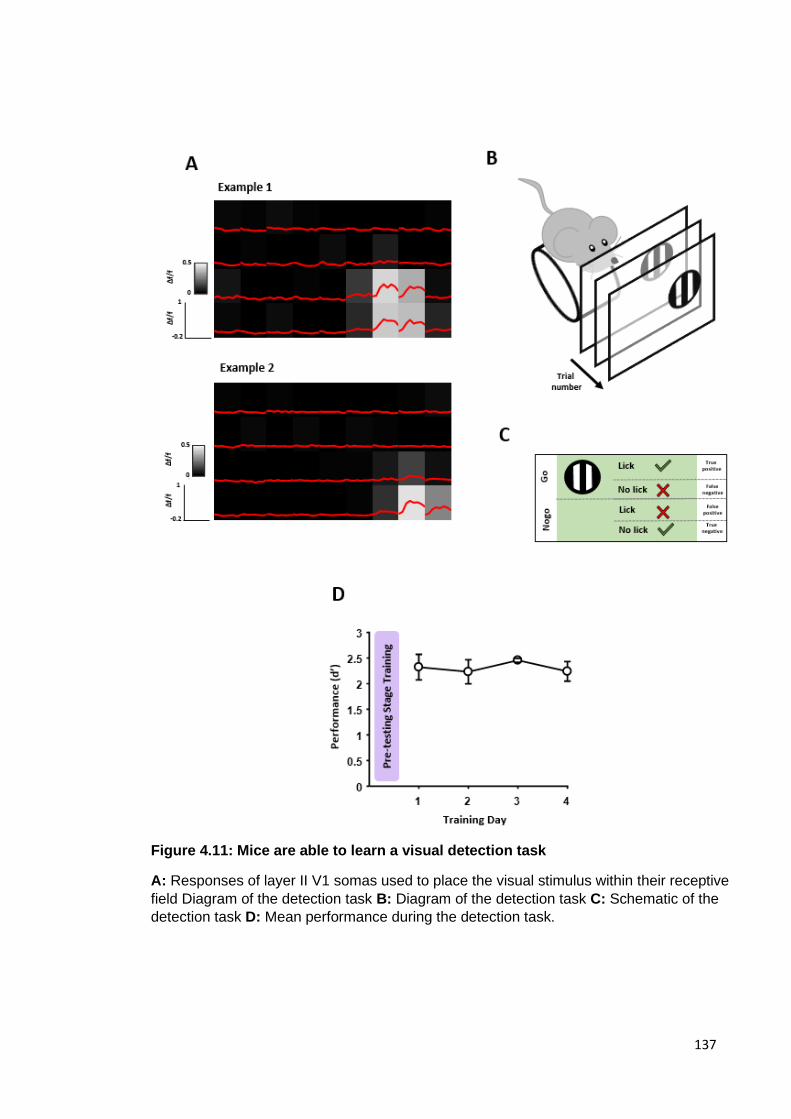
137
Figure 4.11: Mice are able to learn a visual detection task
A: Responses of layer II V1 somas used to place the visual stimulus within their receptive
field Diagram of the detection task B: Diagram of the detection task C: Schematic of the
detection task D: Mean performance during the detection task.
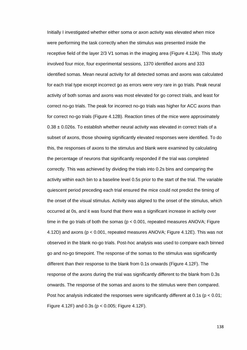
138
Initially I investigated whether either soma or axon activity was elevated when mice
were performing the task correctly when the stimulus was presented inside the
receptive field of the layer 2/3 V1 somas in the imaging area (Figure 4.12A). This study
involved four mice, four experimental sessions, 1370 identified axons and 333
identified somas. Mean neural activity for all detected somas and axons was calculated
for each trial type except incorrect go as errors were very rare in go trials. Peak neural
activity of both somas and axons was most elevated for go correct trials, and least for
correct no-go trials. The peak for incorrect no-go trials was higher for ACC axons than
for correct no-go trials (Figure 4.12B). Reaction times of the mice were approximately
0.38 ± 0.026s. To establish whether neural activity was elevated in correct trials of a
subset of axons, those showing significantly elevated responses were identified. To do
this, the responses of axons to the stimulus and blank were examined by calculating
the percentage of neurons that significantly responded if the trial was completed
correctly. This was achieved by dividing the trials into 0.2s bins and comparing the
activity within each bin to a baseline level 0.5s prior to the start of the trial. The variable
quiescent period preceding each trial ensured the mice could not predict the timing of
the onset of the visual stimulus. Activity was aligned to the onset of the stimulus, which
occurred at 0s, and it was found that there was a significant increase in activity over
time in the go trials of both the somas (p < 0.001, repeated measures ANOVA; Figure
4.12D) and axons (p < 0.001, repeated measures ANOVA; Figure 4.12E). This was not
observed in the blank no-go trials. Post-hoc analysis was used to compare each binned
go and no-go timepoint. The response of the somas to the stimulus was significantly
different than their response to the blank from 0.1s onwards (Figure 4.12F). The
response of the axons during the trial was significantly different to the blank from 0.3s
onwards. The response of the somas and axons to the stimulus were then compared.
Post hoc analysis indicated the responses were significantly different at 0.1s (p < 0.01;
Figure 4.12F) and 0.3s (p < 0.005; Figure 4.12F).

139
The activity of the somas appeared to increase directly in response to the appearance
of the visual stimulus, but the responses of the axons were delayed by approximately
0.3s, aligning more with the reaction time of the mice. This suggested that the
response of ACC axons occurred at the time of or even just before the lick response
rather than the appearance of the visual stimulus itself, as well as only occurring in
correct trials with the motor response of licking. To examine this in more detail, the
activity of the somas and axons was aligned to the rewarded lick. Significantly different
responses between somas and axons were found at -0.1s, 0.1s and 0.3s (p < 0.05, p <
0.05, p < 0.05 respectively). It was interesting to note that ACC axons responded later
in the trial compared to V1 somas, but that this response began slightly before the
animal licked the spout to obtain a reward (Figure 4.12G).

140
Figure 4.12: V1 soma and ACC axon response when stimulus is presented inside the receptive field
A: Example response profile of a V1 soma to 36 different locations and diagram of the visual
stimulus being placed within this receptive field. B: Mean activity trace including all identified
V1 somas (left) and ACC axons (right) divided by trial type. C: Mean reaction times. D/E: The
percentage of V1 Somas (D) and ACC axons (E) showing significantly increased activity in
comparison to a baseline during 0.2 s length bins throughout the trial, aligned to stimulus
onset at 0s F/G: The activity of layer II V1 somas compared to ACC axons where trials were
extracted aligned to the onset of the visual stimulus (F) or the rewarded lick (G). The number
of experimental sessions, mice and detected axons and somas are summarised in Table 6.
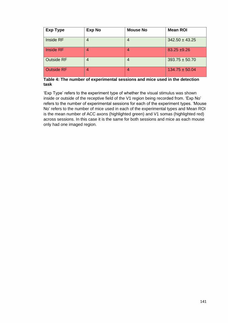
141
Exp Type Exp No Mouse No Mean ROI
Inside RF 4 4 342.50 ± 43.25
Inside RF 4 4 83.25 ±9.26
Outside RF 4 4 393.75 ± 50.70
Outside RF 4 4 134.75 ± 50.04
Table 4: The number of experimental sessions and mice used in the detection task
‘Exp Type’ refers to the experiment type of whether the visual stimulus was shown
inside or outside of the receptive field of the V1 region being recorded from. ‘Exp No’
refers to the number of experimental sessions for each of the experiment types. ‘Mouse
No’ refers to the number of mice used in each of the experimental types and Mean ROI
is the mean number of ACC axons (highlighted green) and V1 somas (highlighted red)
across sessions. In this case it is the same for both sessions and mice as each mouse
only had one imaged region.

142
This analysis was repeated for somas located in a different retinotopic location of V1
that did not respond to the area of visual space in which the stimulus was presented
(Figure 4.13A). This study involved four mice, four experimental sessions, 1575
identified axons and 539 identified somas. The mean activity of all identified ACC
axons again showed that the highest peak in activity was during correct go trials, and
the lowest in correct no-go trials. There was also elevated activity in ACC axons during
incorrect no-go trials. Unexpectedly, V1 somas also exhibited elevated neural activity in
correct go trials even though the visual stimulus was not presented inside their
receptive field (Figure 4.13B). Reaction time was 0.43 ± 0.085s (Figure 4.13C). Next,
V1 somas and ACC axons that significantly responded during correct go or no-go trials
were identified as before. Again, there was a significant increase in activity over the
course of the trial for both the somas (p < 0.05, repeated measures ANOVA; Figure
4.13D) and the ACC axons (p < 0.005, repeated measures ANOVA; Figure 4.13E).
Again, this was not observed for the blank. This indicated the lack of general elevated
activity during correct trials was apparent regardless of whether the stimulus was
presented within or outside the receptive field that matched the imaged retinotopic
location. Post hoc analysis showed significantly increased activity in ACC axons from
0.3s onwards in trials aligned to the visual stimulus onset (Figure 4.13E), something
that was comparable to that observed when the stimulus was presented within the
receptive field. The soma response was, however, not comparable, showing
significantly elevated activity at 0.3s instead of 0.1s. The percentage of ACC axons or
V1 somas significantly responding throughout the trial was not significantly different at
any time point, regardless of whether trials were aligned to the visual stimulus onset
(Figure 4.13F) or the rewarded lick (Figure 4.13G).

143
Figure 4.13: V1 soma and ACC axon response when stimulus is presented outside the receptive field
A: Example response profile of a V1 soma to 36 different locations and diagram of the visual
stimulus being placed outside this receptive field. B: Mean activity trace including all
identified V1 somas (left) and ACC axons (right) divided by trial type. C: Mean reaction
times. D/E: The percentage of V1 Somas (D) and ACC axons (E) showing significantly
increased activity in comparison to a baseline during 0.2 s length bins throughout the trial,
aligned to stimulus onset at 0s F/G: The activity of layer II V1 somas compared to ACC
axons where trials were extracted aligned to the onset of the visual stimulus (F) or the
rewarded lick (G). The number of experimental sessions, mice and detected axons and
somas are summarised in Table 6.

144
4.3.6 Association of ACC activity and lick activity
Each of the previous studies in this chapter have indicated an association between
ACC axon activity in layer 1 V1 and the lick response. Firstly, a significantly higher
percentage of ACC axons exhibited significantly elevated activity in correct go trials
where licking the spout was required, compared to correct no-go trials where it was not.
Furthermore, in all variants of the go/no-go visual discrimination task tested, axons that
had significantly differing activity levels in correct and incorrect trials also exhibited
elevated activity during incorrect no-go trials as well as correct go trials. The common
element between these was the animal licking the spout. Additionally, during the
detection task, ACC activity was not significantly elevated at the time of stimulus onset,
but became so at 0.3s, a delay in time similar to that of reaction time. Motor activity is
known to increase neural activity in many regions of the brain (Niell and Stryker, 2010;
Keller et al., 2012; Bennett et al., 2013; Saleem et al., 2013; Erisken et al., 2014).
Previous studies have shown an integration of motor information into sensory cortices
by looking at the activity of V1 neurons (Pakan et al., 2016). I therefore asked whether
the observed ACC activity was primarily as a result of licking behaviour.
To explore this, the activity of ACC axons was examined during stage one of the
behavioural task where no visual stimuli had been presented. ACC activity was
compared to lick frequency using correlational analysis and a permutation test. To
achieve this a correlation coefficient was calculated between the ACC activity trace and
lick frequency data for the entire session matched over time. The neural activity trace
was then shifted 99 times circularly in time to calculate coefficients of unmatched time
epochs. If the correlation coefficient of the time-matched traces was in the top fifth
percentile of all values then the axon was deemed to be significantly correlated with lick
frequency. It was found that 30.54 ± 0.81% of ACC axons were significantly correlated.

145
Next, this was tested for each the retinotopically predictable, retinotopically
unpredictable and detection tasks It was found that the activity of 31.88 ± 1.91%, 34.43
± 4.34% and 27.67 ± 2.85% of axons were significantly associated with lick frequency
(Figure 4.15A/B/C) in each of the three tasks respectively.
Figure 4.14: ACC activity is linked to lick response before any learning has occurred
A: Correlation coefficients for ACC axon activity and lick frequency. Axons found to be
significantly positively correlated with lick frequency are shown in yellow. B: Example lick
frequency trace (right top); this was aligned to neural activity of each axon significantly
correlated with lick frequency (right middle) and average axon activity (right bottom). This
experiment consisted of five mice and five experimental sessions. There were a mean of
67.20 ± 6.44 axons per experimental session.

146
Figure 4.15: Correlation of ACC axon neural activity and lick frequency
A: For the retinotopically predictable discrimination task, lick frequency was compared with
ACC axon activity. Axons that were found to be significantly positively correlated with lick
frequency using a permutation test are shown in yellow (left). Example lick frequency trace
(right top) where green lines indicated rewarded lick timing; this was aligned to neural activity
of each axon significantly correlated with lick frequency (right middle) and average axon
activity (right bottom) B: As in A but for the retinotopically unpredictable discrimination task
C: As in B but for the visual detection task.

147
ACC axon activity exhibited during the detection task began slightly before the onset of
the licking behaviour suggesting a preparatory response. To investigate this, a cross
correlation was run for axons in both the discrimination and detection tasks to identify
any lag time of lick activity compared to neural activity. The neural traces were then
shifted in time by their lag time and run through the permutation test described
previously. Axons where lick activity was significantly associated with neural activity
were then taken forward and their lag times examined. It was found that in each of the
behavioural tasks the peak lag was -0.49 ± 0.069s, -0.32 ± 0.089s and -0.36 ± 0.059s
for the retinotopically predictable discrimination task, the retinotopically unpredictable
discrimination task and the detection task respectively (Figure 4.16A/B/C). This
indicated that neural activity was occurring in each case before licking activity in axons
that were significantly associated with lick. Furthermore, somas where the stimulus was
shown within the receptive field in the detection task were examined in the same way
and exhibited a peak lag of 0.18 ± 0.095s suggesting that the axons might be exhibiting
a preparatory response.
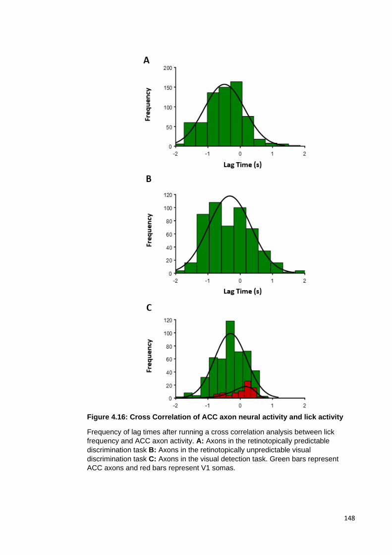
148
Figure 4.16: Cross Correlation of ACC axon neural activity and lick activity
Frequency of lag times after running a cross correlation analysis between lick
frequency and ACC axon activity. A: Axons in the retinotopically predictable
discrimination task B: Axons in the retinotopically unpredictable visual
discrimination task C: Axons in the visual detection task. Green bars represent
ACC axons and red bars represent V1 somas.

149
After establishing an association between ACC activity and the lick response, it was
asked whether ACC axons are associated with locomotion, a motor-related behaviour
that was irrelevant to the successful completion of the task. To do this, mice were
allowed to run or remain stationary at their own discretion and the resulting ACC axonal
activity was compared to run speed using the correlational and permutational analysis
described previously. It was found that the activity of 22.48 ± 6.05% axons were
significantly associated with locomotion.
Figure 4.17: ACC activity is linked to locomotion
A: Correlation coefficients for ACC axon activity and locomotion. Axons found to be
significantly positively correlated with locomotion are shown in yellow. B: Example
locomotion trace (right top); this was aligned to neural activity of each axon significantly
correlated with locomotion (right middle) and average axon activity (right bottom). This
experiment consisted of

150
4.3.7 ACC activity is associated with reward processing
Elevated activity in ACC has been demonstrated to be aligned with motor responses in
human studies involving selective visual attention, especially under conditions of
increased response competition (Carter et al., 1998). This chapter has indicated that
the activity of a subset of ACC axons that terminate in layer 1 V1 in mice are also
associated with the motor response to the task – that of licking. ACC has, however,
also been associated with reward processing (Dehkordi et al., 2015; Liu et al., 2016),
something that would accompany licks in go trials during each behavioural task
presented. It was asked whether this ACC activity associated with licking the spout was
independent of gaining a reward. To do this, each rewarded and each quiescent lick
was identified, and the equivalent ACC neural activity compared for each axon
individually for each behavioural task. It was found that, in all tasks, there were subsets
of axons that had significantly higher responses to rewarded licks compared to
unrewarded licks (Figure 4.18B/C/D). These subsets were then compared to each
other. It was found that a significantly higher percentage of ACC axons responded to
the rewarded lick (p < 0.001, p < 0.01, p < 0.05 for the retinotopically predictable
discrimination, the retinotopically unpredictable discrimination and the detection task
respectively). This suggested an involvement in reward processing.

151
Figure 4.18: ACC axon neural activity is associated with reward
A: Example lick trace where rewarded licks are indicated by a red circle B: Comparison of
ACC axon response to rewarded lick compared to quiescent lick in the retinotopically
predictable task. Each dot represents one axon. Axons responding significantly more to
rewarded licks compared to quiescent licks and vice versa are shown in green and blue
respectively (left) and this is quantified (right) C: As in B but for the retinotopically
unpredictable visual discrimination task D: As in B but for the visual detection task. The
mean number of axons per experimental session is outlined in Table 4.1

152
Exp Type Mouse
number
Exp
Number
Axons per
Mouse
Axons per
Exp
Retinotopically
Predictable
6 16 89.50 ± 7.50 35.8 ± 9.59
Retinotopically
Unpredictable
6 9 68.67 ± 18.32 41.2 ± 12.96
Detection 4 4 97.25 ± 19.51 97.25 ± 19.51
Table 4.1: The mean number of axons per mouse and per experiment identified as significantly responding to lick

153
4.4 Summary of Findings
1. Significantly more axons were active during correct go trials compared to
incorrect go trials.
2. For axons that had significantly different levels of activity in correct trials
compared to incorrect trials, this activity was higher in correct compared to
incorrect go trials, but lower in correct compared to incorrect no-go trials, and
this difference was significant.
3. Making the appearance of the visual stimulus unpredictable and thus
increasing the difficulty of the task did not result in generally elevated ACC
activity during correct trials.
4. Reducing the contrast to make the perception of the visual stimulus more
difficult did not result in generally elevated ACC activity during correct trials.
5. Reducing stimulus size and precisely retinotopically matching the stimulus
location to the imaged area of V1 did not result in elevated ACC activity either.
6. ACC axonal activity appears be associated with the lick response.
7. Activity of a subset of ACC axons is associated with reward.

154
5 General Discussion
5.1 Summary of Studies
The aim of these studies was to investigate the properties of the top-down projection
from ACC to V1. To do this, two main questions were asked. The first was whether
ACC axons in V1 showed any functional organisation where spatial preferences of
axons matched those of V1 somas in the same area of V1. I found that RFCs of ACC
axons carried signals about stimuli appearing across a larger area of visual space than
V1 somas in the same location responded to, and that ACC axon RFCs were offset
horizontally compared to V1 somas. This was different to the retinotopic organisation
properties of the LM projection to V1, one that has been previously shown to exhibit
functional organisation in V1.
The second question was whether an elevation of activity in ACC axons resulted in
improved performance in a visually-guided discrimination task. I found that an
improvement in performance in this task was not associated with an endogenous
general increase in ACC activity. In fact, ACC axon activity appeared to be closely
aligned with the behavioural response of licking, and possibly modulated further by
obtaining a reward during this time.
5.2 Functional Organisation of anterior cingulate cortex and lateral
medial cortex axons terminating in primary visual cortex
5.2.1 ACC axons lack retinotopic organisation but over-represent the horizontal
plane relative to V1 somas in the same retinotopic location in V1
It was found that a subset of ACC axons responded to specific areas in visual
space, but that the proportion was significantly less than V1 somas. The RFCs of
these ACC axons appeared to be spread widely across the visual area in which

155
stimuli were presented indicating that this top-down projection from ACC conveyed
information about a wider range of visual space than the V1 somas located in the
same area of V1.
The RFC offset values of ACC axon RFCs compared to the RFC mean of somas in
the same retinotopic location in V1 over-represented the horizontal place. This
suggested that ACC axons converging on V1 prefer visual space to the left and
right of visual space the V1 somas that they are likely making synapses with prefer.
This functional organisation of ACC axons was not as expected. It has been shown
that this projection is spatially specific (Zhang et al., 2014; Fiser et al., 2016), and
that it is involved in selective visual attention (Zhang et al., 2014). In order to be
able to modulate V1 responses in a spatial specific way to elicit activity observed in
attentional states, it seems logical that the retinotopic arrangement of ACC axons
would match closely to those of V1 pyramidal neurons. The current study does not
show this, instead ACC axons appear to transmit signals driven by stimuli
appearing across the extent of visual space that was tested. One explanation is
that this is because the mouse is passively viewing stimuli. It is possible that this
expected functional organisation of ACC axons is not seen in this experiment
because it does not require the mice to direct visual attention to a specific area of
visual space, and that this organisation may either be observable or develop during
tasks requiring spatial visual attention.
5.2.2 LM axons show retinotopic organisation and over-represent the area of
visual space binocular to V1 somas in the same retinotopic location in
RFCs of LM axons were similarly scattered in azimuth compared to V1 somas, but
significantly more so in elevation. This indicated that LM axons matched RFC

156
scatter properties of the V1 somas in the same area of V1 in azimuth, but
conveyed information about a wider visual area in elevation. RFC offset values of
LM axons compared to those of V1 somas in the same retinotopic location in V1
over-represented the region of visual space in the binocular direction. There was
also a slight bias to higher regions in elevation. This differed from Marques et al.,
(2018) who showed that, on average, V1 somas and LM axons responded to the
same area of visual space. My findings may be as a result of imaging V1 somas
directly to calculate their retinotopic preferences rather than estimating them,
resulting in consistently being able to measure the difference in RFC at a higher
resolution. This binocular bias was observed regardless of whether imaging took
place in monocular or binocular V1. Mice that were reared in the dark and thus had
no visual experience until after two months of age did not show this over-
representation. This offset, coupled with the development of motion perception
requiring visual experience to develop (Mitchell, Kennie and Kung, 2009; Bos,
Gainer and Feller, 2016) suggests that LM conveys information about objects
moving through visual space from the binocular to the monocular receptive field,
and that the organisation needed for this to happen requires visual experience to
develop.
The LM projection to V1 may be important in predicting the movement of objects.
One form of motion processing that this would facilitate would be the movement of
stimuli that occurs in the environment as a result of the movement of the mouse
itself. Marques et al., (2018) argue that the LM projection to V1 could be involved in
motion perception and that it may be specialised for processing movement of
stimuli during locomotion. It is possible that LM projections to V1 encode spatial
predictions back to V1 (Marques et al., 2018), and the offset in the binocular
direction observed in the current study would support this for processing objects

157
moving in the nasal to temporal direction, something that occurs to stationary
objects during locomotion. Figure 5.1 indicates a circuitry that could be behind this.
A stimulus in a particular location in visual space would elicit a response in the
retinotopically matched area of V1, which is reciprocally connected to LM (Wang
and Burkhalter, 2007) and transmits visual information to LM (Glickfeld et al., 2013)
which is reflected in the response profiles of the pyramidal neurons located in LM
(Andermann et al., 2010). This would result in the activity of LM neurons being
directly driven by this visual stimulus. If the stimulus were to then move through
visual space in the monocular direction, something that would be predictable due
to self-motion, then LM axons can send prediction signals of where the stimulus is
likely to be. This would result in LM axons at the imaging area being driven by
stimuli that appear earlier in the path of motion of the object, i.e. towards the
binocular field of view.

158
Figure 5.1: A schematic of the theoretical network involved in the prediction of object movement by LM
A stimulus grating is shown with its path of motion indicated by an arrow and dotted
outline. Yellow lines indicated the path of the light which would stimulate the bottom-
up pathway described in the general introduction and stimulate retinotopically
relevant V1 somas (red). This signal would then be transmitted on to neurons in LM
(green) before being transmitted back to somas in V1 in a retinotopically relevant
position to where the stimulus is likely to move to. Imaging in this area would be one
explanation for the LM RFC offset observed.

159
Another explanation would be processing of the movement of objects, such as that
of incoming aerial predators. Mouse behaviour can be driven by the threat of
predation and consists of two main responses – freezing or fleeing (De Franceschi
et al., 2016). Studies have shown that when mice are presented with a looming
stimulus above them that increases in size thus simulating an incoming aerial
predator, mice respond quickly by fleeing (Yilmaz and Meister, 2013;
De Franceschi et al., 2016). The offset of LM RFCs from those of V1 somas in the
binocular direction coupled with a significantly increased scatter in elevation could
allow mice to track the movement of a visual stimulus approaching from in front
and above them, predict its movement and subsequently make a fast response to
evade predation.
Further experimental work will be needed to determine if the LM projection to V1 is
involved in either processing stationary stimuli that appear to move as the mouse runs,
or with detecting approaching moving objects, such as predators. The former
explanation would involve a form of encoding spatial predictions and can be
manipulated to produce errors in visual processing which may be reflected in the
activity of the projection from LM to V1. One experimental design would be to allow a
mouse to navigate a virtual corridor where the movement of the visual environment is
matched to the movement of the mouse while imaging from LM axons and V1 somas
simultaneously, something that has been shown to work effectively (Poort et al., 2015;
Fiser et al., 2016). If LM axons in V1 were delivering predictive information about
stimuli during motion of the mouse, then it can be hypothesised that these axons would
be active prior to V1 neurons in the same area of visual space. Use of virtual reality
would then allow the visual environment to be reversed so that visual stimuli move in
the opposite direction to what is expected during movement. If LM axons predict
movement in the binocular to monocular direction then it could be hypothesised that

160
this delay would not be seen. To explore the predatory theory further, the fleeing
behaviour of the mouse when faced with an incoming stimulus could be taken
advantage of. The first step would be to image in the same region as before and again
look for a response of LM axons prior to that of V1 neurons, as well as examine
whether animals run in response to the stimulus. LM axons could then be inhibited,
possibly using optogenetics, as was done with ACC axons (Zhang et al., 2014), to see
whether the animal was less likely to flee, or the reaction time before fleeing was
increased.
5.3 The involvement of anterior cingulate cortex axons terminating in
primary visual cortex in visually guided tasks
This study was undertaken to ask whether endogenous elevation of the ACC projection
to V1 was associated with an increase in performance in a visual discrimination task.
Previous experimental work carried out by Zhang et al. (2014) suggested a role for
ACC axons in selective visual attention. An attentional response is believed to
modulate V1 neurons by increasing their response to relevant stimuli and decreasing it
to irrelevant stimuli. Zhang et al. (2014) demonstrated that optogenetically stimulating
ACC axons in layer 1 V1 led to an increase in V1 neuron firing rate to stimuli of the
preferred orientation. As well as this, varying the stimulation distance from the V1
neuron in which the response was being recorded from resulted in a surround-
suppression-like effect. Both of these are hallmarks of visual attention. They argue that
ACC axons are able to modulate both excitatory and inhibitory axonal behaviour
through synapsing with pyramidal cells and interneurons involved in this network. A
further effect of optogenetically stimulating ACC was improved performance in a visual
discrimination task, suggesting these attentional properties of ACC axons are involved.
This study, however, did not show whether mice are able to recruit this projection under
natural conditions.

161
To explore whether this ACC to V1 projection was recruited in the same way under
natural conditions, mice completed a go/no-go visual discrimination task whilst
GCaMP6s-transfected ACC axons were recorded from in V1. I hypothesised that ACC
activity would be elevated when the task was being completely correctly, regardless of
the trial type. The results are discussed below.
5.3.1 There are more active ACC axons during correct go trials than in correct
no-go trials
If the ACC to V1 projection carries an attentional signal and generally elevated ACC
activity is associated with improved performance on a discrimination task then it could
be hypothesised that (a) ACC activity would be greater during trials when the mice
have learned the relevance of each stimuli and (b) ACC activity during correct trials
would be comparable, regardless of the trial type. I found that significantly more ACC
axons responded during the go trial when the mice performed well on the task
compared to when the go trial was first encountered and thus the stimulus had not yet
been associated with a reward. On the other hand, ACC activity during the no-go trial
was comparable. As well as this, significantly more ACC axons had significantly
elevated activity in correct go trials compared to correct no-go trials. This suggested
that performing the task correctly was not associated with an endogenous blanket
elevation in ACC axon activity during correct trials that would have been comparable to
the optogenetic activation of ACC. It has previously been shown that V1 neuronal
responses to stimuli directly associated with a reward are increased compared to those
not associated, and that this association sharpens the tuning of the neurons to their
preferred stimulus (Schoups et al., 2001; Goltstein et al., 2013). This preferential
response to a stimulus with a learned association with a reward is likely to be
influenced by top-down processing and so it would not be unreasonable to consider
162
that the ACC, a projection that emanates from a structure involved in reward
processing, may be modulating this.
5.3.2 ACC axons that discriminate between correct and incorrect trials show
elevated activity during correct go and incorrect no-go trials
Even though significantly more ACC axons exhibited elevated activity during correct
completions of go trials compared to correct no-go trials, this did not rule out that their
activity was greater compared to incorrect trials. Therefore, it was hypothesised that, if
a blanket elevation of ACC axons resulted in improved performance on the visual
discrimination task, then ACC axon activity would be elevated in correct trials,
regardless of trial type. To test this, a group of ACC axons with significantly differing
activity during correct and incorrect trials were identified, and their activity during
incorrect trials was subtracted from that during correct trials. Activity of these axons
was elevated in correct compared to incorrect iterations of go trials, which was in line
with the hypothesis. Unexpectedly, however, the opposite was true for no-go trials. This
suggested that, not only was there no blanket elevation in ACC activity when the task
was being performed correctly, but also that ACC axons were responsive to something
occurring during the incorrect no-go trial. As most activity was observed to occur during
the response window, this could have been as a result of the motor response of licking
the spout, a response to the air puff or even the detection of an unexpected outcome to
the trial.
Furthermore, if ACC axons were involved in visual attention, it would be expected that
the timing of their response would align with the presentation of the visual stimulus.
Fiser et al. (2016) demonstrated that ACC axons in mice exhibited predictive
responses to visual stimuli once they had learned their spatial location by navigating a

163
virtual corridor. In my task the appearance of the visual stimulus was predictable once
the auditory cue was sounded, but axons with differing activity in correct and incorrect
trials did not show significant changes until 2.4s after the presentation of the visual
stimulus, during the response window. This suggested that this population of ACC
axons were not involved in the initial perception of the visual stimulus, but instead
recruited during the part of the task requiring a behavioural response.
5.3.3 General elevated activity is not observed when the visual discrimination
task is more difficult
On the other hand, it has been shown that an ACC projection to claustrum is only
active when the cognitive demands of the task are high enough (Carter et al., 2018).
Optogenetic activation of ACC by Zhang et al. (2014) may have induced a modulation
that is only required in more natural conditions when a task is sufficiently difficult, which
may not have been the case when using a retinotopically predictable task with 100%
stimulus contrast and thus did not recruit the visual attentional properties of this ACC to
V1 projection. To increase task difficulty initially, the task was adapted to a
retinotopically unpredictable one. In this task structure, mice were unable to Mice were
able to learn this task and reach high levels of performance after approximately 14-15
training sessions. This was longer than the time taken on the retinotopically predictable
task, and the mice never reached the same peak performance, confirming the
increased task difficulty.
Using this method, it was possible to ask whether ACC axon responses were spatially
specific, as well as whether there was an elevation of activity across correctly
completed trials. Similar to the retinotopically predictable task, more ACC axons
showed a significant elevation in activity during go trials compared to no-go trials,

164
although this was less pronounced when the stimulus appeared on the ipsilateral side
to imaging. As a greater amount of activity was observed in the go trials, these were
then used to explore whether ACC axons exhibited spatially specific responses.
Significantly more ACC axons significantly responded during go trials regardless of
whether the stimulus was presented on the contralateral or ipsilateral side of the
imaged hemisphere during the trial and especially during the response window.
Furthermore, even with this more difficult task, axons which responded significantly
differently to correct and incorrect trials also exhibited significantly more activity in
correct go and incorrect no-go trials compared to incorrect go and correct no-go trials
respectively. These data suggest a number of things. Firstly, the ACC projection does
not appear to be spatially specific, something that would be necessary for spatial
attentional modulation. Furthermore, even with the increased difficulty, there was no
blanket elevation of ACC activity during correct trials. This was examined further by
increasing the difficulty of perceiving the visual stimulus by reducing the visual stimulus
contrast. Mice were still just able to perform the task but committed more errors. Even
after this, ACC activity was significantly elevated in incorrect no-go compared to correct
no-go trials, particularly during the response window of the task. This provided further
evidence that the endogenous activity of the ACC to V1 projection was unlikely to
contribute to improved performance in a visual discrimination task by indiscriminate
elevation in activity.
5.3.4 Changing the task and stimulus properties did not result in an attentional
signal
There was a possibility that ACC axons were spatially specific and that they exhibit
elevated activity levels when performing well in visually guided tasks but the large
nature of the stimuli in the discrimination task reduced this effect. Modulation of
attention is also believed to involve surround suppression. This is thought to counteract

165
irrelevant stimuli that appear within or close to the location of the attended stimulus that
could elicit a response that would ultimately degrade that to the attended stimulus.
Zhang et al. (2014) showed that the ACC to V1 projection is spatially specific and that it
exhibits activity comparable to surround suppression. Therefore, the attentional
response might have been missed by presenting a large stimulus in the same location
in both go and no-go trials, as well as not presenting the stimulus in a location of visual
space precisely matched to the retinotopically relevant area of V1. To address these
points, a detection task with a smaller stimulus where both ACC axons and L2/3
pyramidal somas were recorded from simultaneously was used.
In this task, both V1 somas and ACC axons responded significantly more to the
stimulus presentation than to the blank in correct trials, again suggesting that there is
not a blanket elevation in ACC activity when performing correctly compared to
incorrectly in a visually guided attention task. Interestingly, upon appearance of the
stimulus, significantly more V1 somas responded in comparison to ACC axons, but the
proportion became comparable 0.4s later, in between the onset of the visual stimulus
and the reaction time. This suggested that the ACC axons are driven by the motor
response associated with the reward rather than being involved in the initial perception
and guiding of selective visual attention to the stimulus, and that the signal may be
preparatory. This would be in line with studies that have suggested ACC is involved in
the response element of visually guided tasks
5.3.5 ACC axon activity is associated with the lick behavioural response
Each of the previous findings strongly suggest that high performance in a visually
guided discrimination task is not associated with a complementary endogenous blanket
elevation in ACC activity. It was found that in the discrimination task that there were

166
significantly more ACC axons active during correct go trials compared to correct no-go
trials, that ACC axons responded more to correct go trials compared to incorrect go
trials and that ACC axons responded more to incorrect no-go trials than correct no-go
trials. In the detection task it was found that ACC axon activity was delayed until after
the stimulus, suggesting it is not directly involved in the perception of the visual
stimulus. In fact, it aligned more closely with the behavioural response indicating an
involvement with the motor response rather than the perception of the visual stimulus
itself. Taken together these data suggest that the principal factor driving activity of ACC
axons in V1 was licking behaviour. Analysis of the precise relationship of ACC axon
activity to licking behaviour indicated that a fraction of axons were significantly
correlated. Furthermore, this activity appeared to occur just before the lick behaviour
which suggested a preparatory signal. Previous studies in humans have suggested that
ACC plays a role in visually guided tasks that require selective attention, and that its
activity is elevated specifically during the response element of the task (Pardo et al.,
1990; Carter et al., 1998). Taken together, this suggests that ACC is involved in the
visual discrimination task, but not the direct perception of the stimulus. Instead, it plays
a role in directing the behavioural response to that stimulus. This would also explain
why its activity did not appear to depend on the location in which the stimulus was
presented (Pardo et al., 1990; Carter et al., 1998; MacDonald et al., 2005).
5.3.6 ACC axon activity is influenced by reward
By comparing the responses of ACC axons to either a rewarded or unrewarded lick, it
was found that a fraction of axons had a significantly higher response to one of the two.
Furthermore, significantly more axons preferred licks that were rewarded. This
suggested that ACC activity was not simply associated with just the lick response, but
instead that rewarded licks and non-rewarded licks were processed differently. One
such system would be the integration of visual and motor information for the successful

167
timing of the reward. It has been shown that, over the course of associating a visual
stimulus with a reward, a substantial proportion of V1 neurons begin to predict the
timing of the reward (Shuler and Bear, 2006), and activity within V1 is coupled to lick
responses when animals must make this motor response based on a visual stimulus
(Namboodiri et al., 2015). Reward timing is thought to be influenced by top-down
processing and rely on cholinergic inputs projecting from the basal forebrain (Chubykin
et al., 2013). ACC receives a substantial input of this kind (Zaborszky et al., 2015). Its
activity is linked to licking, reflecting the changes observed in V1, but also to the
outcome of the lick, suggesting that it is able to integrate information about the visual
stimulus and the outcome of the response in order to aid the mouse in making the
correct response during a visually guided task. Further study will need to be carried out
to explore the possible role of this ACC to V1 projection in reward timing.
5.3.7 Further study into the role of the ACC to V1 projection in visually guided
tasks
It could be argued that visual discrimination tasks do not fully test attentional responses
as there are no distractors to ignore presented at the same time as either stimulus.
Optogenetic stimulation of ACC axons by Zhang et al., (2014) during a visual
discrimination task could have led to an artificially induced improvement in performance
due to the addition of an attention signal that is not required or attainable under
endogenous conditions. It may, therefore, be interesting to further explore a possible
role for ACC axons projecting to V1 in attention. One way of doing this would be to
introduce distractors into the behaviour. Stimuli would appear in two or more locations,
one of which was previously cued. The mouse would then have to pay attention to the
stimulus that appears in the cued location and respond accordingly, regardless of the
type of stimuli which appear in the other locations. Another approach would be to
explore using other tasks believed to engage attention. It has been shown that mice

168
are able to perform the 5-choice serial reaction time task (5-CSRTT) where animals
must respond to unpredictable visual stimuli presented in one of five locations. This
task is thought to measure both attention and motor impulsivity (Higgins and Silenieks,
2017). With the advancement of two-photon imaging in freely moving mice (Helmchen,
Denk and Kerr, 2013; Ozbay et al., 2018), this type of experiment may not even need
to be adapted to head-fixed animals. Using these types of task would not only allow
further exploration of attention, but have also been adapted from tasks used with
humans (Higgins and Silenieks, 2017). Deficits in attention have been linked to
neuropsychiatric conditions such as schizophrenia. Understanding the mechanisms
that underlie attention could ultimately help in understanding the pathology of these
conditions, and so it is important to design experiments that they are as relevant as
possible across species.
On the other hand, it would be interesting to probe the role of ACC axons in the
behavioural responses further. A major question here is whether ACC axon activity
would be elevated depending on the type of motor behavioural response, especially if
that response is not directly linked with a reward. One way to explore this would be to
image ACC axons while mice undertake a visually guided task requiring a different
behavioural response. An example would be where mice are taught to turn a steering
wheel to make two alternative choices similar to that in Burgess et al. (2017). This task
would involve two motor behaviours, the first being the turning of the wheel in response
to an identified visual stimulus. The second would be licking a spout to acquire a
reward if this is done correctly. This would result in a task encompassing ACC activity
in response to perceiving a visual stimulus, a motor behavioural response that is not
licking and is not directly associated with a reward, and the motor response of licking
that is associated with a reward that each occur at temporally defined times.
Furthermore, it would be interesting to inhibit the activity of ACC axons using

169
optogenetics once any behaviour task has been learned to explore whether it is
alleviated.
5.3.8 Methodological drawbacks of the techniques used
There are a number of methodological drawbacks of the techniques used throughout
this thesis that must be understood alongside considering the work presented here.
Firstly, although the use of calcium indicators is a powerful technique that allows
hundreds of neurons to be imaged down to the level of a single bouton or dendrite, it
has several disadvantages against other techniques, for example electrophysiology.
One of these is that fluorescence fluctuations are simply a proxy of neuronal activity.
This, coupled with the slow decay of the signal, means that the use of this technique
does not directly measure neuronal activity, and if the study requires action potential to
be identified then this can only be done by modelling methods including deconvolution.
It also means that it may not be possible to see subtle and quick changes in neuronal
firing patterns that can be observed with electrophysiology. It is important, therefore,
that experiments are designed with this in mind. On top of this, light is scattered
through the tissue using this technique meaning it can only be used at fairly superficial
depths (Girven and Sparta, 2017), this is however being circumnavigated using
wavelengths of light less subject to scatter (Dana et al., 2016) and by using
microprisms (Andermann et al., 2013). On the other hand, even with the advent of
multi-region electrophysiological recordings using polymer electrode assays (Chung et
al., 2019), two-photon calcium imaging of calcium indicators has the ability to record
from much larger populations of neurons simultaneously (Jercog et al., 2016),
something of great importance in understanding how the brain works as an entire
network in the years to come.

170
Another drawback of these methods is the use of mice to understand the visual
system. The mouse visual system is less complex than that of humans and so using it
as a model in very controlled settings could be viewed as reductionist. On the other
hand, it is possible to record neuronal activity down to the resolution of single axons
using mice, something that s not currently possible using scanning techniques with
humans. It is also possible to get a much higher throughput of data. Furthermore, there
are a huge number of sophisticated tools available for experimental studies such as
genetic modification, injection of viruses and the use of optogenetics to manipulate
specific cell types and circuits (Huberman and Niell, 2011; Ellenbroek and Youn, 2016).
It is important to keep in mind both the huge advantages and criticisms of using two-
photon imaging in freely moving mice to study networks in the brain in order to design
robust experiments and interpret the results with integrity.
5.3.9 Concluding remarks
Overall, the data presented here indicates that the ACC projection to V1 is involved in
visually guided tasks but is associated more with the motor response of licking than the
perception of the visual stimulus. The additional modulation by reward suggests that
this association depends upon the outcome of trials and may therefore be important for
behaviours such as reward timing.

171
6 References
Andermann, M. L. et al. (2013) ‘Chronic Cellular Imaging of Entire Cortical Columns in
Awake Mice Using Microprisms’, Neuron, 80(4), pp. 900–913.
Andermann, M. L., Kerlin, A. M. and Reid, R. C. (2010) ‘Chronic cellular imaging of
mouse visual cortex during operant behavior and passive viewing.’, Frontiers in cellular
neuroscience, 4, p. 3.
de Araujo, I. E. T. et al. (2003) ‘Human cortical responses to water in the mouth, and
the effects of thirst.’, Journal of neurophysiology. American Physiological Society,
90(3), pp. 1865–76.
Baden, T. et al. (2016) ‘The functional diversity of retinal ganglion cells in the mouse’,
Nature. Nature Publishing Group, 529(7586), pp. 345–350.
Barch, D. M. et al. (2012) ‘The clinical translation of a measure of gain control: the
contrast-contrast effect task.’, Schizophrenia bulletin. Oxford University Press, 38(1),
pp. 135–43.
Baumeister, A. A. and Francis, J. L. (2002) ‘Historical development of the dopamine
hypothesis of schizophrenia.’, Journal of the history of the neurosciences, 11(3), pp.
265–77.
Beauchamp, M. S. et al. (2001) ‘A Parametric fMRI Study of Overt and Covert Shifts of
Visuospatial Attention’, NeuroImage. Academic Press, 14(2), pp. 310–321.
Bennett, C., Arroyo, S. and Hestrin, S. (2013) ‘Subthreshold mechanisms underlying
state-dependent modulation of visual responses.’, Neuron. Elsevier, 80(2), pp. 350–7.
Bisley, J. W. and Goldberg, M. E. (2010) ‘Attention, Intention, and Priority in the
Parietal Lobe’, Annual Review of Neuroscience.
Blakemore, C. and Tobin, E. (1972) ‘Lateral inhibition between orientation detectors in

172
the cat’s visual cortex’, Experimental Brain Research. Springer-Verlag, 15(4), pp. 439–
440.
Bos, R., Gainer, C. and Feller, M. B. (2016) ‘Role for Visual Experience in the
Development of Direction-Selective Circuits.’, Current biology : CB. NIH Public Access,
26(10), pp. 1367–75.
Braff, D. L. (1993) ‘Information processing and attention dysfunctions in
schizophrenia.’, Schizophrenia bulletin, 19(2), pp. 233–59.
Brefczynski, J. A. and DeYoe, E. A. (1999) ‘A physiological correlate of the “spotlight”
of visual attention’, Nature Neuroscience. Nature Publishing Group, 2(4), pp. 370–374.
Broersen, L. . and Uylings, H. B. . (1999) ‘Visual attention task performance in Wistar
and Lister Hooded rats: response inhibition deficits after medial prefrontal cortex
lesions’, Neuroscience. Pergamon, 94(1), pp. 47–57.
Broussard, G. J. et al. (2018) ‘In vivo measurement of afferent activity with axon-
specific calcium imaging’, Nature Neuroscience. Nature Publishing Group, 21(9), pp.
1272–1280.
Brown, H. et al. (2013) ‘Active inference, sensory attenuation and illusions’, Cognitive
Processing. Springer Berlin Heidelberg, 14(4), pp. 411–427.
Butler, P. D., Silverstein, S. M. and Dakin, S. C. (2008) ‘Visual Perception and Its
Impairment in Schizophrenia’, Biological Psychiatry. Elsevier, 64(1), pp. 40–47.
Cang, J. et al. (2005) ‘Ephrin-As Guide the Formation of Functional Maps in the Visual
Cortex’, Neuron. Cell Press, 48(4), pp. 577–589.
Carter, A. M. et al. (2018) ‘Anterior Cingulate Cortex Input to the Claustrum Is Required
for Top-Down Action Control’, Cell Reports.
Carter, C. S. et al. (1998) ‘Anterior Cingulate Cortex, Error Detection, and the Online

173
Monitoring of Performance’, Science. American Association for the Advancement of
Science, 280(5364), pp. 747–749.
Carter, J. D. et al. (2010) ‘Attention deficits in schizophrenia--preliminary evidence of
dissociable transient and sustained deficits.’, Schizophrenia research. NIH Public
Access, 122(1–3), pp. 104–12.
Chen, J. L. et al. (2013) ‘Imaging neuronal populations in behaving rodents: paradigms
for studying neural circuits underlying behavior in the mammalian cortex.’, The Journal
of neuroscience : the official journal of the Society for Neuroscience, 33(45), pp.
17631–40.
Chen, T.-W. et al. (2013) ‘Ultrasensitive fluorescent proteins for imaging neuronal
activity.’, Nature. Nature Publishing Group, a division of Macmillan Publishers Limited.
All Rights Reserved., 499(7458), pp. 295–300.
Chen, Y. et al. (2008) ‘Task difficulty modulates the activity of specific neuronal
populations in primary visual cortex’, Nature Neuroscience. Nature Publishing Group,
11(8), pp. 974–982.
Chubykin, A. A. et al. (2013) ‘A cholinergic mechanism for reward timing within primary
visual cortex.’, Neuron. NIH Public Access, 77(4), pp. 723–35.
Chung, J. E. et al. (2019) ‘High-Density, Long-Lasting, and Multi-region
Electrophysiological Recordings Using Polymer Electrode Arrays’, Neuron. Cell Press,
101(1), pp. 21-31.e5.
Clark, A. (2013) ‘Whatever next? Predictive brains, situated agents, and the future of
cognitive science’, Behavioral and Brain Sciences, 36(03), pp. 181–204.
Cocker, P. J. et al. (2016) ‘Activation of dopamine D4 receptors within the anterior
cingulate cortex enhances the erroneous expectation of reward on a rat slot machine
task.’, Neuropharmacology, 105, pp. 186–95.

174
Coleman, M. J. et al. (2009) ‘Schizophrenia Patients Show Deficits in Shifts of Attention
to Different Levels of Global-Local Stimuli: Evidence for Magnocellular Dysfunction’,
Schizophrenia Bulletin. Narnia, 35(6), pp. 1108–1116.
Corbetta, M. et al. (1991) ‘Selective and Divided Attention during Visual Discriminations
of Shape, Color, and Speed: Functional Anatomy by Positron Emission Tomography’,
The Journal of Neuroscience, 1(9), pp. 2393–2402.
Corbetta, M. and Shulman, G. L. (2002) ‘Control of goal-directed and stimulus-driven
attention in the brain’, Nature Reviews Neuroscience. Nature Publishing Group, 3(3),
pp. 201–215.
Coyle, J. T. (2012) ‘NMDA receptor and schizophrenia: a brief history.’, Schizophrenia
bulletin. Oxford University Press, 38(5), pp. 920–6.
Dakin, S., Carlin, P. and Hemsley, D. (2005) ‘Weak suppression of visual context in
chronic schizophrenia.’, Current biology : CB. Elsevier, 15(20), pp. R822-4.
Daliri, M. R., Kozyrev, V. and Treue, S. (2016) ‘Attention enhances stimulus
representations in macaque visual cortex without affecting their signal-to-noise level’,
Scientific Reports.
Dana, H. et al. (2016) ‘Sensitive red protein calcium indicators for imaging neural
activity’, eLife, 5.
De Franceschi, G. et al. (2016) ‘Vision Guides Selection of Freeze or Flight Defense
Strategies in Mice’, Current Biology. Cell Press, 26(16), pp. 2150–2154.
Dehaene, S. et al. (2003) ‘Conscious and subliminal conflicts in normal subjects and
patients with schizophrenia: The role of the anterior cingulate’, Proceedings of the
National Academy of Sciences of the United States of America. National Academy of
Sciences, 100(23), p. 13722.
Dehkordi, O. et al. (2015) ‘Neuroanatomical circuitry mediating the sensory impact of

175
nicotine in the central nervous system.’, Journal of neuroscience research, 93(2), pp.
230–43.
Desimone, R. and Duncan, J. (1995) ‘NEURAL MECHANISMS OF SELECTIVE
VISUAL ATTENTION’, Annu. Rev. Neurosci, 18, pp. 193–222.
Dipoppa, M. et al. (2018) ‘Vision and Locomotion Shape the Interactions between
Neuron Types in Mouse Visual Cortex.’, Neuron. Elsevier, 98(3), pp. 602-615.e8.
Dräger, U. C. (1975) ‘Receptive fields of single cells and topography in mouse visual
cortex’, Journal of Comparative Neurology. John Wiley & Sons, Ltd, 160(3), pp. 269–
289.
Dum, R. P. and Strick, P. L. (1991) ‘The origin of corticospinal projections from the
premotor areas in the frontal lobe.’, The Journal of neuroscience : the official journal of
the Society for Neuroscience. Society for Neuroscience, 11(3), pp. 667–89.
Ellenbroek, B. and Youn, J. (2016) ‘Rodent models in neuroscience research: Is it a rat
race?’, DMM Disease Models and Mechanisms. Company of Biologists Ltd, 9(10), pp.
1079–1087.
Erisken, S. et al. (2014) ‘Effects of locomotion extend throughout the mouse early
visual system.’, Current biology : CB. Elsevier, 24(24), pp. 2899–907.
Feldheim, D. A. and O’Leary, D. D. M. (2010) ‘Visual map development: bidirectional
signaling, bifunctional guidance molecules, and competition.’, Cold Spring Harbor
perspectives in biology. Cold Spring Harbor Laboratory Press, 2(11), p. a001768.
Filinger, C. et al. (2018) 'Efferents of anterior cingulate areas 24a and 24b and
midcingulate areas 24a' and 24b' in the mouse.', Brain Structure and Function. 223(4),
p1747-1778
Fioravanti, M. et al. (2005) ‘A meta-analysis of cognitive deficits in adults with a
diagnosis of schizophrenia’, Neuropsychology Review.

176
Fiser, A. et al. (2016) ‘Experience-dependent spatial expectations in mouse visual
cortex’, Nature Neuroscience.
Friston, K. (2005) ‘A theory of cortical responses.’, Philosophical transactions of the
Royal Society of London. Series B, Biological sciences. The Royal Society, 360(1456),
pp. 815–36.
Friston, K. J. (1998) ‘The disconnection hypothesis’, Schizophrenia Research. Elsevier,
30(2), pp. 115–125.
Garrett, M. E. et al. (2014) ‘Topography and areal organization of mouse visual cortex.’,
The Journal of neuroscience : the official journal of the Society for Neuroscience,
34(37), pp. 12587–600.
Geisler, S. et al. (2007) ‘Glutamatergic afferents of the ventral tegmental area in the
rat.’, The Journal of neuroscience : the official journal of the Society for Neuroscience.
Society for Neuroscience, 27(21), pp. 5730–43.
Girven, K. S. and Sparta, D. R. (2017) ‘Probing Deep Brain Circuitry: New Advances in
in Vivo Calcium Measurement Strategies.’, ACS chemical neuroscience, 8(2), pp. 243–
251.
Glickfeld, L. L. et al. (2013) ‘Cortico-cortical projections in mouse visual cortex are
functionally target specific’, Nature Neuroscience. Nature Publishing Group, 16(2), pp.
219–226.
Goard, M. J. et al. (2016) ‘Distinct roles of visual, parietal, and frontal motor cortices in
memory-guided sensorimotor decisions’, eLife. eLife Sciences Publications Limited, 5,
pp. 471–477.
Goldstein, E. B. (1981) ‘The Ecology of J. J. Gibson’s Perception’, Leonardo, 14(3), p.
191.
Goltstein, P. M. et al. (2013) ‘In vivo two-photon Ca2+ imaging reveals selective reward

177
effects on stimulus-specific assemblies in mouse visual cortex.’, The Journal of
neuroscience : the official journal of the Society for Neuroscience. Society for
Neuroscience, 33(28), pp. 11540–55.
Goltstein, P. M., Meijer, G. T. and Pennartz, C. M. (2018) ‘Conditioning sharpens the
spatial representation of rewarded stimuli in mouse primary visual cortex’, eLife, 7.
Goodale, M. A. and Milner, A. D. (1992) ‘Separate visual pathways for perception and
action’, Trends in Neurosciences. Elsevier Current Trends, 15(1), pp. 20–25.
Green, M. F. et al. (1999) ‘Backward masking in unmedicated schizophrenic patients in
psychotic remission: possible reflection of aberrant cortical oscillation.’, The American
journal of psychiatry, 156(9), pp. 1367–73.
Gregoriou, G. G. et al. (2014) ‘Lesions of prefrontal cortex reduce attentional
modulation of neuronal responses and synchrony in V4’, Nature Neuroscience. Nature
Publishing Group, 17(7), pp. 1003–1011.
Hahn, B., Ross, T. J. and Stein, E. A. (2007) ‘Cingulate Activation Increases
Dynamically with Response Speed under Stimulus Unpredictability’, Cerebral Cortex.
Narnia, 17(7), pp. 1664–1671.
Harris, K. D. and Shepherd, G. M. G. (2015) ‘The neocortical circuit: Themes and
variations’, Nature Neuroscience. Nature Publishing Group, pp. 170–181.
Helmchen, F., Denk, W. and Kerr, J. N. D. (2013) ‘Miniaturization of two-photon
microscopy for imaging in freely moving animals.’, Cold Spring Harbor protocols. Cold
Spring Harbor Laboratory Press, 2013(10), pp. 904–13.
Higgins, G. A. and Silenieks, L. B. (2017) ‘Rodent Test of Attention and Impulsivity: The
5-Choice Serial Reaction Time Task’, in Current Protocols in Pharmacology. Hoboken,
NJ, USA: John Wiley & Sons, Inc., pp. 5.49.1-5.49.34.
Histed, M. H., Carvalho, L. A. and Maunsell, J. H. R. (2012) ‘Psychophysical

178
measurement of contrast sensitivity in the behaving mouse’, Journal of
Neurophysiology. American Physiological Society Bethesda, MD, 107(3), pp. 758–765.
Hoonakker, M., Doignon-Camus, N. and Bonnefond, A. (2017) ‘Sustaining attention to
simple visual tasks: a central deficit in schizophrenia? A systematic review’, Annals of
the New York Academy of Sciences. John Wiley & Sons, Ltd (10.1111), 1408(1), pp.
32–45.
Hubel, D. H. and Wiesel, T. N. (1968) ‘Receptive fields and functional architecture of
monkey striate cortex’, The Journal of Physiology. John Wiley & Sons, Ltd (10.1111),
195(1), pp. 215–243.
HUBEL, D. H. and WIESEL, T. N. (1959) ‘Receptive fields of single neurones in the
cat’s striate cortex.’, The Journal of physiology. Wiley-Blackwell, 148(3), pp. 574–91.
HUBEL, D. H. and WIESEL, T. N. (1962) ‘Receptive fields, binocular interaction and
functional architecture in the cat’s visual cortex.’, The Journal of physiology. Wiley-
Blackwell, 160(1), pp. 106–54.
Huberman, A. D. and Niell, C. M. (2011) ‘What can mice tell us about how vision
works?’, Trends in Neurosciences, pp. 464–473.
Iacaruso, M. F., Gasler, I. T. and Hofer, S. B. (2017) ‘Synaptic organization of visual
space in primary visual cortex’, Nature, 547(7664), pp. 449–452.
Isomura, Y. et al. (2003) ‘Neural coding of "attention for action" and
"response selection" in primate anterior cingulate cortex.’, The Journal of
neuroscience : the official journal of the Society for Neuroscience. Society for
Neuroscience, 23(22), pp. 8002–12.
Jercog, P., Rogerson, T. and Schnitzer, M. J. (2016) ‘Large-Scale Fluorescence
Calcium-Imaging Methods for Studies of Long-Term Memory in Behaving Mammals.’,
Cold Spring Harbor perspectives in biology. Cold Spring Harbor Laboratory Press, 8(5),
179
p. a021824.
Jiang, X. et al. (2015) ‘Principles of connectivity among morphologically defined cell
types in adult neocortex’, Science. American Association for the Advancement of
Science, 350(6264), p. aac9462.
Juavinett, A. L. et al. (2016) ‘Automated identification of mouse visual areas with
intrinsic signal imaging’, Nature Protocols. Nature Research, 12(1), pp. 32–43.
Jurjut, O. et al. (2017) ‘Learning Enhances Sensory Processing in Mouse V1 before
Improving Behavior’, Journal of Neuroscience. Society for Neuroscience, 37(27), pp.
6460–6474.
Kalatsky, Valery A and Stryker, M. P. (2003) ‘New paradigm for optical imaging:
temporally encoded maps of intrinsic signal.’, Neuron. Elsevier, 38(4), pp. 529–45.
Kalatsky, Valery A. and Stryker, M. P. (2003) ‘New Paradigm for Optical Imaging:
Temporally Encoded Maps of Intrinsic Signal’, Neuron. Cell Press, 38(4), pp. 529–545.
Kastner, S. et al. (1998) ‘Mechanisms of directed attention in the human extrastriate
cortex as revealed by functional MRI.’, Science (New York, N.Y.). American
Association for the Advancement of Science, 282(5386), pp. 108–11.
Kastner, S. and Ungerleider, L. (2000) ‘Mechanisms of Visual Attention in the Human
Cortex’, Annual Review of Neuroscience.
Keller, A. J. et al. (2017) ‘Stimulus relevance modulates contrast adaptation in visual
cortex’, eLife.
Keller, G. B., Bonhoeffer, T. and Hübener, M. (2012) ‘Sensorimotor mismatch signals in
primary visual cortex of the behaving mouse.’, Neuron. Elsevier, 74(5), pp. 809–15.
Kringelbach, M. L. et al. (2003) ‘Activation of the Human Orbitofrontal Cortex to a
Liquid Food Stimulus is Correlated with its Subjective Pleasantness’, Cerebral Cortex,

180
13(10), pp. 1064–1071.
Lee, A. M. et al. (2014) ‘Identification of a brainstem circuit regulating visual cortical
state in parallel with locomotion.’, Neuron. Elsevier, 83(2), pp. 455–466.
Leinweber, M. et al. (2017) ‘A Sensorimotor Circuit in Mouse Cortex for Visual Flow
Predictions’, Neuron. Cell Press, 95(6), pp. 1420-1432.e5.
Li, R. et al. (2018) ‘Two-Photon Functional Imaging of the Auditory Cortex in Behaving
Mice: From Neural Networks to Single Spines’, Frontiers in Neural Circuits. Frontiers,
12, p. 33.
Li, W., Piëch, V. and Gilbert, C. D. (2008) ‘Learning to Link Visual Contours’, Neuron.
Cell Press, 57(3), pp. 442–451.
Liu, C. et al. (2016) ‘Neuronal activity and the expression of hypothalamic oxytocin and
vasopressin in social versus cocaine conditioning.’, Behavioural brain research, 310,
pp. 84–92.
MacDonald, A. W. et al. (2005) ‘Specificity of Prefrontal Dysfunction and Context
Processing Deficits to Schizophrenia in Never-Medicated Patients With First-Episode
Psychosis’, American Journal of Psychiatry. American Psychiatric Publishing, 162(3),
pp. 475–484.
Makino, H. and Komiyama, T. (2015) ‘Learning enhances the relative impact of top-
down processing in the visual cortex’, Nature Neuroscience. Nature Publishing Group,
a division of Macmillan Publishers Limited. All Rights Reserved., 18(8), pp. 1116–1122.
Maldonado, P. E. et al. (1997) ‘Orientation selectivity in pinwheel centers in cat striate
cortex.’, Science (New York, N.Y.). American Association for the Advancement of
Science, 276(5318), pp. 1551–5.
Mangun, G. R. and Hillyard, S. A. (1990) ‘Allocation of visual attention to spatial
locations: Tradeoff functions for event-related brain potentials and detection

181
performance’, Perception & Psychophysics. Springer-Verlag, 47(6), pp. 532–550.
Marques, T. et al. (2018) ‘The functional organization of cortical feedback inputs to
primary visual cortex’, Nature Neuroscience. Nature Publishing Group, 21(5), pp. 757–
764.
Marshel, J. H. et al. (2011) ‘Functional Specialization of Seven Mouse Visual Cortical
Areas’, Neuron. MIT Press, Cambridge, MA, 72(6), pp. 1040–1054.
McAdams, C. J. and Maunsell, J. H. (1999) ‘Effects of attention on orientation-tuning
functions of single neurons in macaque cortical area V4.’, The Journal of
neuroscience : the official journal of the Society for Neuroscience. Society for
Neuroscience, 19(1), pp. 431–41.
Métin, C., Godement, P. and Imbert, M. (1988) ‘The primary visual cortex in the mouse:
receptive field properties and functional organization.’, Experimental brain research,
69(3), pp. 594–612.
Miller, E. K. and Cohen, J. D. (2001) ‘AN INTEGRATIVE THEORY OF PREFRONTAL
CORTEX FUNCTION’.
Mishkin, M., Ungerleider, L. G. and Macko, K. A. (1983) ‘Object vision and spatial
vision: two cortical pathways’, Trends in Neurosciences. Elsevier Current Trends, 6, pp.
414–417.
Mitchell, D. E., Kennie, J. and Kung, D. (2009) ‘Development of Global Motion
Perception Requires Early Postnatal Exposure to Patterned Light’, Current Biology.
Cell Press, 19(8), pp. 645–649.
Miyamoto, D. et al. (2016) ‘Top-down cortical input during NREM sleep consolidates
perceptual memory’, Science.
Mizuno, H., Hirano, T. and Tagawa, Y. (2007) ‘Evidence for Activity-Dependent Cortical
Wiring: Formation of Interhemispheric Connections in Neonatal Mouse Visual Cortex

182
Requires Projection Neuron Activity’, Journal of Neuroscience. Society for
Neuroscience, 27(25), pp. 6760–6770.
Moran, J. and Desimone, R. (1985) ‘Selective attention gates visual processing in the
extrastriate cortex’, Science, (229), pp. 782–784.
Morecraft, R. J. and van Hoesen, G. W. (1992) ‘Cingulate input to the primary and
supplementary motor cortices in the rhesus monkey: Evidence for somatotopy in areas
24c and 23c’, The Journal of Comparative Neurology. John Wiley & Sons, Ltd, 322(4),
pp. 471–489.
Morin, L. P. and Studholme, K. M. (2014) ‘Retinofugal projections in the mouse.’, The
Journal of comparative neurology. NIH Public Access, 522(16), pp. 3733–53.
Motter, B. C. (1994) ‘Neural correlates of attentive selection for color or luminance in
extrastriate area V4.’, The Journal of neuroscience : the official journal of the Society
for Neuroscience. Society for Neuroscience, 14(4), pp. 2178–89.
Murakami, T., Matsui, T. and Ohki, K. (2017) ‘Functional Segregation and Development
of Mouse Higher Visual Areas.’, The Journal of neuroscience : the official journal of the
Society for Neuroscience. Society for Neuroscience, 37(39), pp. 9424–9437.
Namboodiri, V. M. K. et al. (2015) ‘Visually cued action timing in the primary visual
cortex’, Neuron.
Nathanson, J. L. et al. (2009) ‘Preferential labeling of inhibitory and excitatory cortical
neurons by endogenous tropism of adeno-associated virus and lentivirus vectors.’,
Neuroscience. NIH Public Access, 161(2), pp. 441–50.
Neuchterlein, K. H. et al. (1991) ‘9. Information-processing anomalies in the early
course of schizophrenia and bipolar disorder’, Schizophrenia Research. Elsevier, 5(3),
pp. 195–196.
Niell, C. M. and Stryker, M. P. (2008) ‘Highly selective receptive fields in mouse visual

183
cortex.’, The Journal of neuroscience : the official journal of the Society for
Neuroscience. NIH Public Access, 28(30), pp. 7520–36.
Niell, C. M. and Stryker, M. P. (2010) ‘Modulation of Visual Responses by Behavioral
State in Mouse Visual Cortex’, Neuron. Cell Press, 65(4), pp. 472–479.
Ohki, K. et al. (2005) ‘Functional imaging with cellular resolution reveals precise micro-
architecture in visual cortex’, Nature. Nature Publishing Group, 433(7026), pp. 597–
603.
Ozbay, B. N. et al. (2018) ‘Three dimensional two-photon brain imaging in freely
moving mice using a miniature fiber coupled microscope with active axial-scanning’,
Scientific Reports. Nature Publishing Group, 8(1), p. 8108.
Pachitariu, M. et al. (2017) ‘Suite2p: beyond 10,000 neurons with standard two-photon
microscopy’, bioRxiv. Cold Spring Harbor Laboratory, p. 061507.
Pakan, J. M. et al. (2016) ‘Behavioral-state modulation of inhibition is context-
dependent and cell type specific in mouse visual cortex’, eLife, 5.
Pardo, J. V et al. (1990) ‘The anterior cingulate cortex mediates processing selection in
the Stroop attentional conflict paradigm.’, Proceedings of the National Academy of
Sciences of the United States of America. National Academy of Sciences, 87(1), pp.
256–9.
Pfeffer, C. K. et al. (2013) ‘Inhibition of inhibition in visual cortex: the logic of
connections between molecularly distinct interneurons’, Nature Neuroscience. Nature
Publishing Group, 16(8), pp. 1068–1076.
Polack, P.-O., Friedman, J. and Golshani, P. (2013) ‘Cellular mechanisms of brain
state–dependent gain modulation in visual cortex’, Nature Neuroscience. Nature
Publishing Group, 16(9), pp. 1331–1339.
Poort, J. et al. (2015) ‘Learning Enhances Sensory and Multiple Non-sensory

184
Representations in Primary Visual Cortex’, Neuron.
Powers, A. R., Mathys, C. and Corlett, P. R. (2017) ‘Pavlovian conditioning-induced
hallucinations result from overweighting of perceptual priors.’, Science (New York,
N.Y.). American Association for the Advancement of Science, 357(6351), pp. 596–600.
Priebe, N. J. and McGee, A. W. (2014) ‘Mouse vision as a gateway for understanding
how experience shapes neural circuits’, Frontiers in Neural Circuits. Frontiers, 8, p.
123.
Qadir, H. et al. (2018) 'Structural Connectivity of the Anterior Cingulate Cortex,
Claustrum, and the Anterior Insula of the Mouse.', Frontiers in Neuroanatomy. 26 p.
100
Ranson, A. et al. (2019) ‘Top-Down Suppression of Sensory Cortex in an NMDAR
Hypofunction Model of Psychosis’, Schizophrenia Bulletin.
Rao, R. P. N. and Ballard, D. H. (1999) ‘Predictive coding in the visual cortex: a
functional interpretation of some extra-classical receptive-field effects’, Nature
Neuroscience. Nature Publishing Group, 2(1), pp. 79–87.
Rauss, K. and Pourtois, G. (2013) ‘What is Bottom-Up and What is Top-Down in
Predictive Coding?’, Frontiers in psychology. Frontiers Media SA, 4, p. 276.
Reynolds, J. H., Chelazzi, L. and Desimone, R. (1999) ‘Competitive mechanisms
subserve attention in macaque areas V2 and V4.’, The Journal of neuroscience : the
official journal of the Society for Neuroscience. Society for Neuroscience, 19(5), pp.
1736–53.
Reynolds, J. H., Pasternak, T. and Desimone, R. (2000) ‘Attention increases sensitivity
of V4 neurons.’, Neuron. Elsevier, 26(3), pp. 703–14.
Ringach, D. L. et al. (2016) ‘Spatial clustering of tuning in mouse primary visual cortex’,
Nature Communications. Nature Publishing Group, 7(1), p. 12270.

185
Rolls, E. T. and McCabe, C. (2007) ‘Enhanced affective brain representations of
chocolate in cravers vs. non-cravers’, European Journal of Neuroscience. Blackwell
Publishing Ltd, 26(4), pp. 1067–1076.
Rubio-Garrido, P. et al. (2009) ‘Thalamic Input to Distal Apical Dendrites in Neocortical
Layer 1 Is Massive and Highly Convergent’, Cerebral Cortex. Narnia, 19(10), pp. 2380–
2395.
Saleem, A. B. et al. (2013) ‘Integration of visual motion and locomotion in mouse visual
cortex’, Nature Neuroscience. Nature Publishing Group, 16(12), pp. 1864–1869.
Schoups, A. et al. (2001) ‘Practising orientation identification improves orientation
coding in V1 neurons’, Nature. Nature Publishing Group, 412(6846), pp. 549–553.
Schweimer, J. and Hauber, W. (2005) ‘Involvement of the rat anterior cingulate cortex
in control of instrumental responses guided by reward expectancy.’, Learning &
memory (Cold Spring Harbor, N.Y.), 12(3), pp. 334–42.
Sengpiel, F., Sen, A. and Blakemore, C. (1997) ‘Characteristics of surround inhibition in
cat area 17.’, Experimental brain research, 116(2), pp. 216–28.
Shidara, M. and Richmond, B. J. (2002) ‘Anterior Cingulate: Single Neuronal Signals
Related to Degree of Reward Expectancy’, Science, 296(5573).
Shima, K. (1998) ‘Role for Cingulate Motor Area Cells in Voluntary Movement Selection
Based on Reward’, Science. American Association for the Advancement of Science,
282(5392), pp. 1335–1338.
Shuler, M. G. and Bear, M. F. (2006) ‘Reward timing in the primary visual cortex.’,
Science (New York, N.Y.). American Association for the Advancement of Science,
311(5767), pp. 1606–9.
Smith, I. T. et al. (2017) ‘Stream-dependent development of higher visual cortical
areas’, Nature Neuroscience. Nature Publishing Group, 20(2), pp. 200–208.

186
Sohya, K. et al. (2007) ‘GABAergic neurons are less selective to stimulus orientation
than excitatory neurons in layer II/III of visual cortex, as revealed by in vivo functional
Ca2+ imaging in transgenic mice.’, The Journal of neuroscience : the official journal of
the Society for Neuroscience. Society for Neuroscience, 27(8), pp. 2145–9.
Spitzer, H., Desimone, R. and Moran, J. (1988) ‘Increased attention enhances both
behavioral and neuronal performance’, Science, 240(4850), pp. 338–340.
Squire, R. F. et al. (2013) ‘Prefrontal Contributions to Visual Selective Attention’,
Annual Review of Neuroscience.
Sundberg, K. A., Mitchell, J. F. and Reynolds, J. H. (2009) ‘Spatial attention modulates
center-surround interactions in macaque visual area v4.’, Neuron. Elsevier, 61(6), pp.
952–63.
Svoboda, K. and Yasuda, R. (2006) ‘Principles of Two-Photon Excitation Microscopy
and Its Applications to Neuroscience’, Neuron. Cell Press, 50(6), pp. 823–839.
Teufel, C. et al. (2015) ‘Shift toward prior knowledge confers a perceptual advantage in
early psychosis and psychosis-prone healthy individuals.’, Proceedings of the National
Academy of Sciences of the United States of America. National Academy of Sciences,
112(43), pp. 13401–6.
Theeuwes, J. (2010) ‘Top–down and bottom–up control of visual selection’, Acta
Psychologica. North-Holland, 135(2), pp. 77–99.
Tootell, R. B. et al. (1998) ‘The retinotopy of visual spatial attention.’, Neuron. Elsevier,
21(6), pp. 1409–22.
Treue, S. and Maunsell, J. (1996) ‘Attentional modulation of visual motion processing in
cortical areas MT and MST’, Nature, (382), pp. 539–541.
Wang, Q. and Burkhalter, A. (2007) ‘Area map of mouse visual cortex.’, The Journal of
comparative neurology, 502(3), pp. 339–57.
187
Wang, Y. et al. (2008) ‘Spatial distribution of cingulate cortical cells projecting to the
primary motor cortex in the rat’, Neuroscience Research. Elsevier, 60(4), pp. 406–411.
Weiss, Y., Simoncelli, E. P. and Adelson, E. H. (2002) ‘Motion illusions as optimal
percepts’, Nature Neuroscience. Nature Publishing Group, 5(6), pp. 598–604.
Williford, T. and Maunsell, J. H. R. (2006) ‘Effects of Spatial Attention on Contrast
Response Functions in Macaque Area V4’, Journal of Neurophysiology. American
Physiological Society, 96(1), pp. 40–54.
Wong, R. O. L., Meister, M. and Shatz, C. J. (1993) ‘Transient period of correlated
bursting activity during development of the mammalian retina’, Neuron. Cell Press,
11(5), pp. 923–938.
Wu, D. et al. (2017) ‘Persistent Neuronal Activity in Anterior Cingulate Cortex
Correlates with Sustained Attention in Rats Regardless of Sensory Modality’, Scientific
Reports. Nature Publishing Group, 7(1), p. 43101.
Wurtz, R. H. (1968) ‘Visual Cortex Neurons: Response to Stimuli during Rapid Eye
Movements’, Science. American Association for the Advancement of Science,
162(3858), pp. 1148–1150.
Yan, Y. et al. (2014) ‘Perceptual training continuously refines neuronal population
codes in primary visual cortex’, Nature Neuroscience. Nature Publishing Group, 17(10),
pp. 1380–1387.
Yilmaz, M. and Meister, M. (2013) ‘Rapid innate defensive responses of mice to
looming visual stimuli’, Current biology : CB. NIH Public Access, 23(20), pp. 2011–5.
Zaborszky, L. et al. (2015) ‘Neurons in the basal forebrain project to the cortex in a
complex topographic organization that reflects corticocortical connectivity patterns: an
experimental study based on retrograde tracing and 3D reconstruction.’, Cerebral
cortex (New York, N.Y. : 1991). Oxford University Press, 25(1), pp. 118–37.

188
Zhang, S. et al. (2014) ‘Selective attention. Long-range and local circuits for top-down
modulation of visual cortex processing.’, Science (New York, N.Y.). American
Association for the Advancement of Science, 345(6197), pp. 660–5.
Zhang, S. et al. (2016) ‘Organization of long-range inputs and outputs of frontal cortex
for top-down control’, Nature Neuroscience.
Zhou, H. and Desimone, R. (2011) ‘Feature-Based Attention in the Frontal Eye Field
and Area V4 during Visual Search’, Neuron.