Embed Size (px)
Citation preview

Page
The Fundamental Theorem

Page 2
GA
Why does it work?
1. Schema Theorem
2. Search Spaces as Hypercubes

Page 3
Schema
A Schema is a similarity template describing a
subset of strings with similarities at certain
string positions.
e.g. For a binary alphabet {0, 1}, we motivate a schema by appending a
special symbol *, or don’t care symbol,
producing a ternary alphabet {0, 1, *} that allows us to build schemata.
We can think of it as a pattern matching device: a
schema matches a particular string if at every location in
the schema a 1 matches a 1 in the string, or a 0 matches
a 0, or a * matches either.
Page
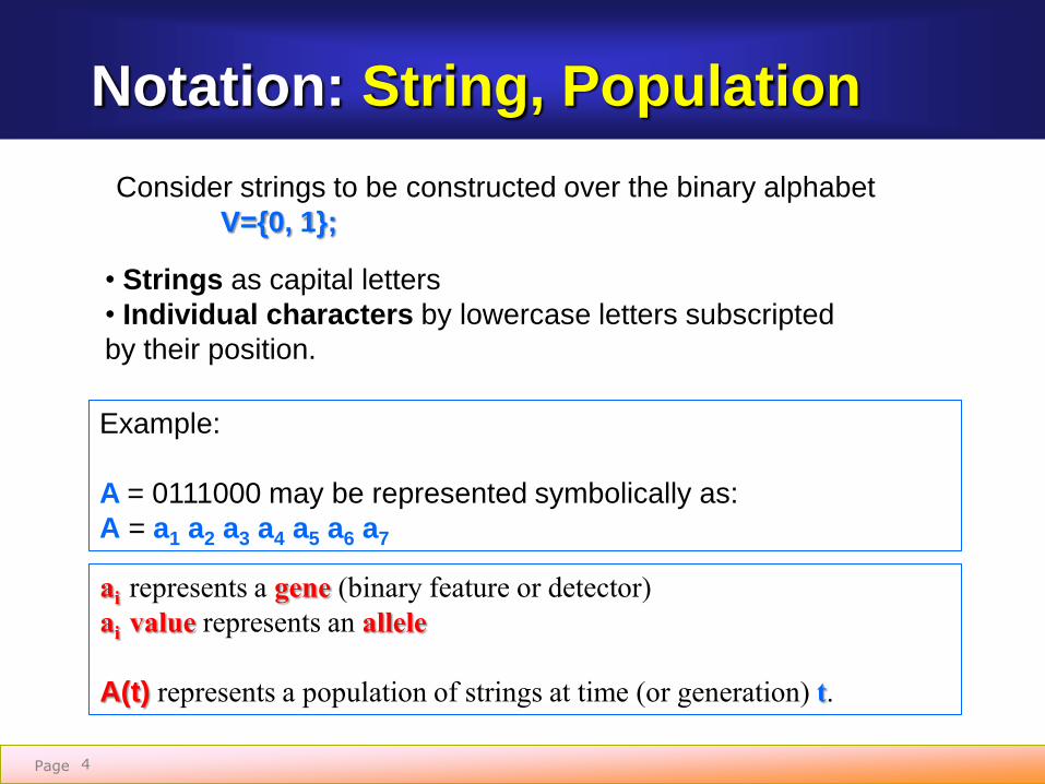
Notation: String, Population
4
Consider strings to be constructed over the binary alphabet
V={0, 1};
• Strings as capital letters
• Individual characters by lowercase letters subscripted
by their position.
Example:
A = 0111000 may be represented symbolically as:
A = a1 a2 a3 a4 a5 a6 a7
ai represents a gene (binary feature or detector)
ai value represents an allele
A(t) represents a population of strings at time (or generation) t.

Page
Notation: Schema
5
Consider a schema H taken from the three-letter
alphabet:
V={ 0, 1, * };
* asterisk is a don’t care symbol which
matches either a 0 or a 1 at a particular
position.

Page 6
Schema Matching
A bit string matches a particular schemata if that
bit string can be constructed from the schemata
by replacing the symbol with the appropriate bit
value.
e.g.
H = *11*0**
String A = 0111000
String A is an example of the schema H
because the string alleles ai match
schema positions hi at the fixed positions
2, 3 and 5.

Page

Page 8
Order of Schema:
o(H) – is the number of fixed positions
present in the template
Understanding the building blocks of future solutions
Schema Properties
Schema Order:
o(011*1**) = 4
Schema Defining Length:
δ(H) = 5-1 = 4011*1**
Schema Order:
o(0******) = 1
0******Schema Defining Length: δ(H) = 0, because
there is only one fixed position
Defining Length of Schema:
δ(H) – is the distance between the first
and last specific string position

Page 9
They provide the basic means for analyzing the net
effect of reproduction and genetic operators on
the building blocks contained within the population.
Understanding the building blocks of future solutions
Schema Properties
Schemata and their properties serve as notational
devices for rigorously discussing and classifying
string similarities.

Page
Page
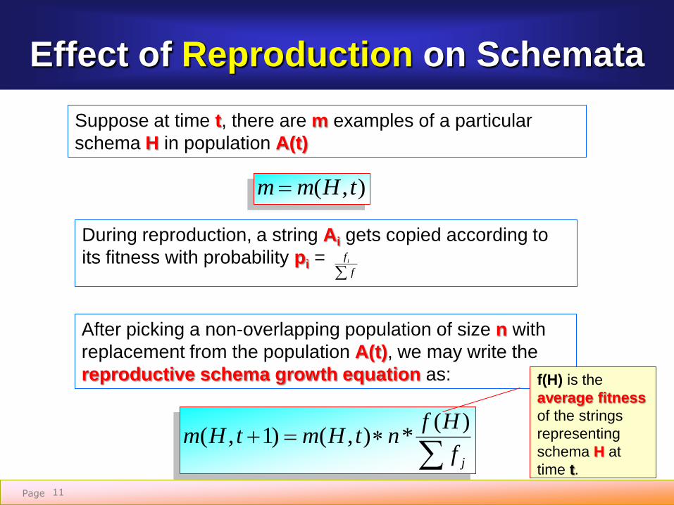
Effect of Reproduction on Schemata
11
Suppose at time t, there are m examples of a particular
schema H in population A(t)
During reproduction, a string Ai gets copied according to
its fitness with probability pi =
After picking a non-overlapping population of size n with
replacement from the population A(t), we may write the
reproductive schema growth equation as:
f
fi
jf
HfntHmtHm
)(*),()1,(
),( tHmm
f(H) is the
average fitness
of the strings
representing
schema H at
time t.

Page 12
If we recognise that the average fitness of the entire
population as we may express the
reproductive schema growth equation as:
After picking a non-overlapping population of size n with replacement from the
population A(t), we may write the reproductive schema growth equation as:
n
ff
jf
HfntHmtHm
)(*),()1,(
f
HftHmtHm
)(*),()1,(
Simplification
Effect of Reproduction on Schemata

Page 13
Reproductive schema growth equation:
f
HftHmtHm
)(*),()1,(
• A particular schema grows as the ratio of the average fitness of the
schema to the average fitness of the population.
• Schemata with fitness values above the population average will receive
an increasing number of samples in the next generation.
• Schemata with fitness values below the population average will receive a
decreasing number of samples.
• All the schemata in a population grow or decay according to their schema
averages under the operation of reproduction alone.
Effect of Reproduction on Schemata

Page 14
Reproductive schema growth equation:
f
HftHmtHm
)(*),()1,(
Suppose we assume that a particular schema H remains above average an
amount with a c constant. Under this assumption, we can write:
Quantitave Effect of Reproduction on Schemata
fc
),(*)1()(
*),()1,( tHmcf
fcftHmtHm
Starting at t=0, and assuming a stationary value of c, we obtain the equation:
tcHmtHm )1(*)0,(),(
Reproduction allocates exponentially increasing (decreasing) numbers of
trials to above (below) average schema.

Page
Reproduction can allocate exponentially increasing and decreasing
numbers of schemata to future generations in parallel.
Many, many different schemata are sampled in parallel according to
the same rule through the use of n simple reproduction operations.
However, reproduction does not promote exploration of new
regions of the search space.
This is where crossover steps in.
Quantitave Effect of Reproduction on Schemata
tcHmtHm )1(*)0,(),(

Page
Consider a particular string of length l = 7 and two representative
schemata within that string:
Effect of Crossover on Schemata
A = 0111000
H1 = *1****0
H2 = ***10**
Recall: Crossover Operation
crossover proceeds with the random selection of a mate;
Random selection of a crossover site, and the exchange of
substrings from the beginning of the string to the crossover site
inclusively with the corresponding substring of the chosen mate.

Page
Consider a particular string of length l = 7 and two representative
schemata within that string:
Effect of Crossover on Schemata
Assuming that we have the following randomly chosen crossover
site: 3
A = 0 1 1 | 1 0 0 0
H1 = * 1 * | * * * 0
H2 = * * * | 1 0 * *
A = 0 1 1 1 0 0 0
H1 = * 1 * * * * 0
H2 = * * * 1 0 * *

Page
Effect of Crossover on Schemata
Assuming that we have the following randomly chosen crossover
site: 3
A = 0 1 1 | 1 0 0 0
H1 = * 1 * | * * * 0
H2 = * * * | 1 0 * *
H1 is destroyed. Defining length = 5
H2 will survive. Defining length = 1
H1 is less likely to survive crossover than schema H2 because on
average the crossover site is more likely to fall between the extreme
fixed positions.

Page
Effect of Crossover on Schemata
A = 0 1 1 | 1 0 0 0
H1 = * 1 * | * * * 0
H2 = * * * | 1 0 * *
H1 is less likely to survive crossover than schema H2 because on average the
crossover site is more likely to fall between the extreme fixed positions.
Let’s quantify this observation. If the crossover site is selected uniformly
at random among the l-1=7-1 = 6 possible sites,
then H1 is destroyed with probability pd and survives with probability ps.
H1 is destroyed. Defining length = 5
H2 will survive. Defining length = 1
6
5
)1(
)(
l
Hpd
6
11 ds ppH1

Page
Effect of Crossover on Schemata
A = 0 1 1 | 1 0 0 0
H1 = * 1 * | * * * 0
H2 = * * * | 1 0 * *
H1 is less likely to survive crossover than schema H2 because on average the
crossover site is more likely to fall between the extreme fixed positions.
If the crossover site is selected uniformly at random among the l-1=7-1 = 6
possible sites. Similarly, you can calculate the probability of destruction and
survival for H2 as follows:
H1 is destroyed. Defining length = 5
H2 will survive. Defining length = 1
6
1
)1(
)(
l
Hpd
6
51 ds ppH2

Page
Lower Bound on Crossover Survival Probability
To generalise, a schema survives when the cross over site falls outside the defining
length. The survival probability under simple crossover is ps
)1(
)(1
l
Hp s
Lower Bound on Crossover
Survival Probability

Page
Lower Bound on Crossover Survival Probability
To generalise, a schema survives when the cross over site falls outside the defining length.
The survival probability under simple crossover is ps
)1(
)(1
l
Hp s
If we consider the probability of performing a crossover operation to be pc,
)1(
)(1
l
Hpp cs
Page
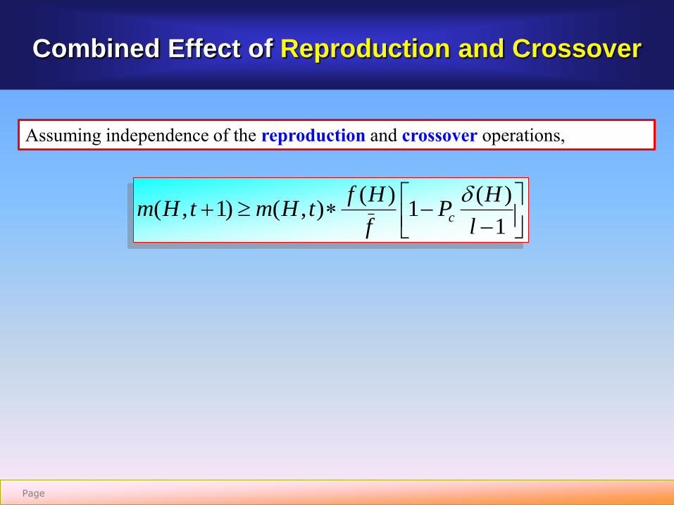
Combined Effect of Reproduction and Crossover
Assuming independence of the reproduction and crossover operations,
1
)(1
)(),()1,(
l
HP
f
HftHmtHm c

Page
Combined Effect of Reproduction and Crossover
Assuming independence of the reproduction and crossover operations,
1
)(1
)(),()1,(
l
HP
f
HftHmtHm c
Schema H grows or decays depending upon a multiplication factor.

Page
Combined Effect of Reproduction and Crossover
Assuming independence of the reproduction and crossover operations,
1
)(1
)(),()1,(
l
HP
f
HftHmtHm c
Schema H grows or decays depending upon a multiplication factor.
That factor depends on 2 things:
• whether the schema is above or below the population average
• whether the schema has relatively short or long defining length.

Page
Combined Effect of Reproduction and Crossover
Assuming independence of the reproduction and crossover operations,
1
)(1
)(),()1,(
l
HP
f
HftHmtHm c
Schema H grows or decays depending upon a multiplication factor.
That factor depends on 2 things:
• whether the schema is above or below the population average
• whether the schema has relatively short or long defining length.ar
Clearly, those schemata with both above-average observed performance and short-
defining lengths are going to be sampled at exponentially increasing rates.

Page
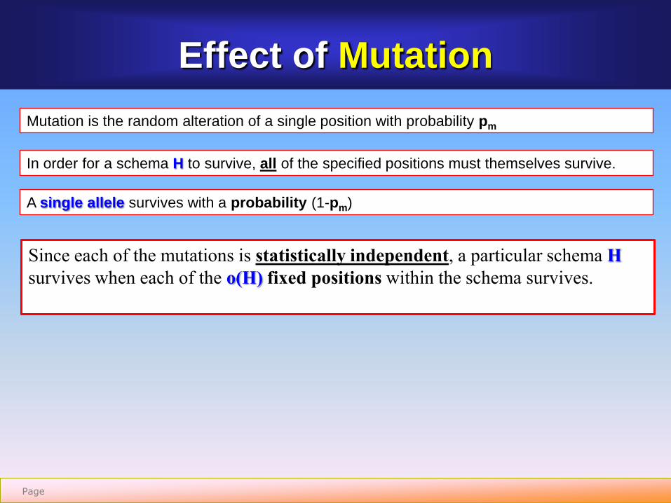
Effect of Mutation
Mutation is the random alteration of a single position with probability pm

Page
Effect of Mutation
Mutation is the random alteration of a single position with probability pm
In order for a schema H to survive, all of the specified positions must themselves
survive.
A single allele survives with a probability (1-pm)
Page
Effect of Mutation
Mutation is the random alteration of a single position with probability pm
In order for a schema H to survive, all of the specified positions must themselves survive.
A single allele survives with a probability (1-pm)
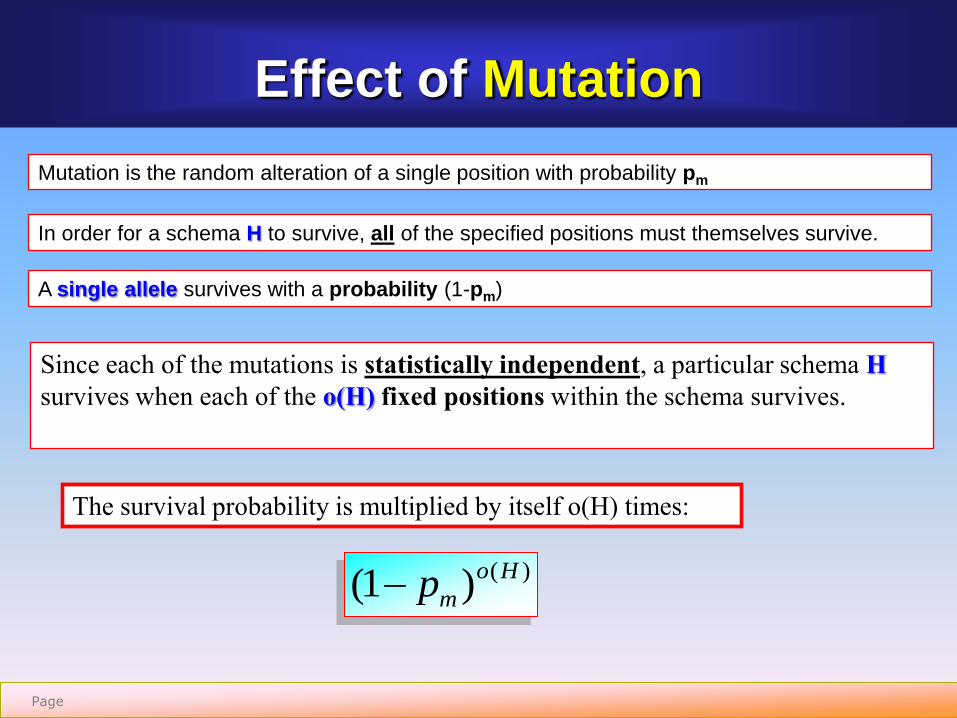
Since each of the mutations is statistically independent, a particular schema H
survives when each of the o(H) fixed positions within the schema survives.
Page
Effect of Mutation
Mutation is the random alteration of a single position with probability pm
In order for a schema H to survive, all of the specified positions must themselves survive.
A single allele survives with a probability (1-pm)
Since each of the mutations is statistically independent, a particular schema H
survives when each of the o(H) fixed positions within the schema survives.
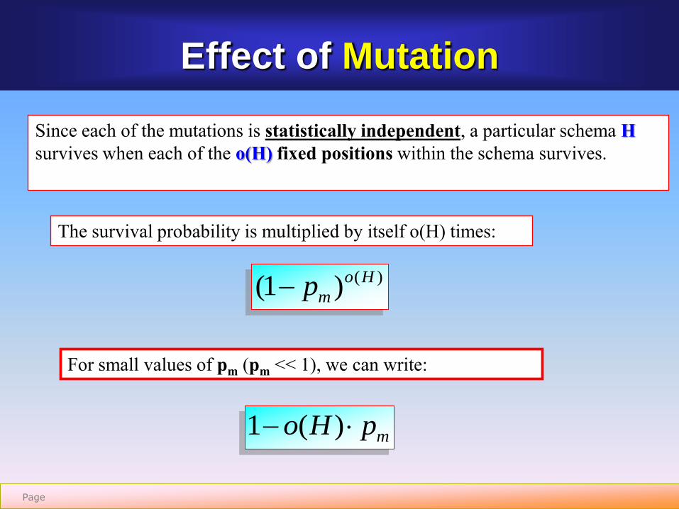
)()1( Ho
mp
The survival probability is multiplied by itself o(H) times:
Page
Effect of Mutation
Since each of the mutations is statistically independent, a particular schema H
survives when each of the o(H) fixed positions within the schema survives.
)()1( Ho
mp
The survival probability is multiplied by itself o(H) times:
For small values of pm (pm << 1), we can write:
mpHo )(1

Page 32
Short, low-order, above-average
schemata are given exponentially increasing
trials in subsequent generations.
Schema TheoremFundamental Theorem of Genetic Algorithms
mc PHo
l
HP
f
HftHmtHm )(
1
)(1
)(),()1,(
Expected Count of Schema
H at time (t+1)
Number of H Schema at
time t
Population average
Schema average
Schema Defining Length
Schema Order
Pc – probability of cross over
Pm – probability of mutation
Who shall live and who shall die?
Let’s verify
this!

Page

Page 34
Schema Processing by hand
Observe the effect of reproduction, crossover,
and mutation.
Let us observe how the GA processes schemata-
not individual strings-within the population.
Let us consider three particular schemata, H1, H2 and H3
Where
• H1 = 1****
• H2 = *10**
• H3 = 1***0

Page 35
String
number
Initial
Population
X value f(x) pselect Expected
count
Actual
count(Roulette
Wheel)
1 01101 13 169 0.14 0.58 1
2 11000 24 576 0.49 1.97 2
3 01000 8 64 0.06 0.22 0
4 10011 19 361 0.31 1.23 1
f
fi
f
f i
GA PROCESSING OF SCHEMATA – Hand Calculations
Sum 1170
Ave. 293
Max. 576
Genetic Algorithm
Schema String
RepresentativesSchema
Average
Fitness f(H)
H1 1**** 2, 4 469
H2 *10** 2, 3 320
H3 1***0 2 576
Schema Processing: Before Reproduction
mc PHo
l
HP
f
HftHmtHm )(
1
)(1
)(),()1,(
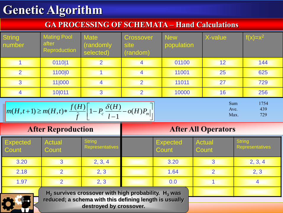
Page 36
String
number
Mating Pool
after
Reproduction
Mate
(randomly
selected)
Crossover
site
(random)
New
population
X-value f(x)=x2
1 0110|1 2 4 01100 12 144
2 1100|0 1 4 11001 25 625
3 11|000 4 2 11011 27 729
4 10|011 3 2 10000 16 256
GA PROCESSING OF SCHEMATA – Hand Calculations
Sum 1754
Ave. 439
Max. 729
Genetic Algorithm
Expected
Count
Actual
Count
String
RepresentativesExpected
Count
Actual
Count
String
Representatives
3.20 3 2, 3, 4 3.20 3 2, 3, 4
2.18 2 2, 3 1.64 2 2, 3
1.97 2 2, 3 0.0 1 4
After All OperatorsAfter Reproduction
H2 survives crossover with high probability. H3 was
reduced; a schema with this defining length is usually
destroyed by crossover.
mc PHo
l
HP
f
HftHmtHm )(
1
)(1
)(),()1,(

Page

Page 38
GA
Why does it work?
Search Spaces as HypercubesThe question that most people who are new to the field of genetic algorithms ask
at this point is why such a process should do anything useful?
Why should one believe that this is going to result in an effective form of search
or optimization?
The answer which is most widely given to explain the computational behavior
of genetic algorithms came out of John Holland’s work. In his classic book,
Adaptation in Natural and Artificial Systems, Holland develops several
arguments designed to explain how a genetic plan or genetic algorithm can
result in complex and robust search by implicitly sampling hyperplane
partitions of a search space.

Page 39
Hyperplane
A hyperplane is a concept in geometry. It is a generalization of the concept of a plane.
In 1-D space (such as a line), a hyperplane is a point; it divides a line into two rays.
In 2-D space (such as the xy plane), a hyperplane is a line; it divides the plane into two half-planes.
In 3-D space, a hyperplane is an ordinary plane; it divides the space into two half-spaces.
This concept can also be applied to four-dimensional space and beyond, where the dividing object is simply referred to as a hyperplane.
http://en.wikipedia.org/wiki/Hyperplane

Page 40
0*1 Line
*0* Plane
1** Plane
*1* Plane11* Line
Points in the space are strings
or schemata of order 3
Visualization of Schemata
as Hyperplanes in 3-D Space
Consider the strings and schemata of length l =3
001
011
010110
100
101
000
111

Page 41
0*1 Line
*0* Plane
1** Plane
*1* Plane11* Line
Points in the space are strings
or schemata of order 3
Lines in the space are schemata or
order 2
Visualization of Schemata
as Hyperplanes in 3-D Space
Consider the strings and schemata of length l =3
001
011
010110
100
101
000
111

Page 42
0*1 Line
*0* Plane
1** Plane
*1* Plane11* Line
Points in the space are strings
or schemata of order 3
Lines in the space are schemata or
order 2
Planes in the space are schemata
of order 1
The whole space is covered by
the schema of order 0, ***
Visualization of Schemata
as Hyperplanes in 3-D Space
Consider the strings and schemata of length l =3
001
011
010110
100
101
000
111

Page 43
Similarity Templates as Hyperplanes
This result generalizes to spaces of higher
dimension where we must abandon the geometrical
notions available to us in 3-D space.
Points, lines, and planes described by schemata in
3-D generalize to hyperplanes of varying
dimension in n-space.
We can think of a GA cutting across different
hyperplanes to search for improved performance.
Page 44
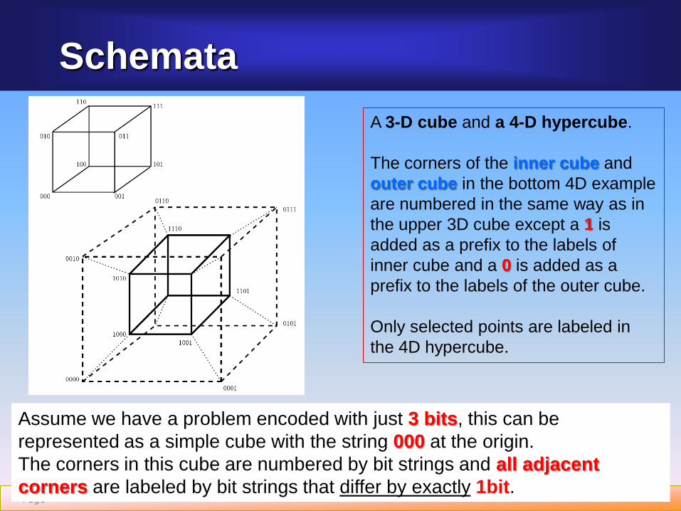
Schemata
A 3-D cube and a 4-D hypercube.
The corners of the inner cube and
outer cube in the bottom 4D example
are numbered in the same way as in
the upper 3D cube except a 1 is
added as a prefix to the labels of
inner cube and a 0 is added as a
prefix to the labels of the outer cube.
Only selected points are labeled in
the 4D hypercube.
Assume we have a problem encoded with just 3 bits, this can be
represented as a simple cube with the string 000 at the origin.
The corners in this cube are numbered by bit strings and all adjacent
corners are labeled by bit strings that differ by exactly 1bit.

Page 45
Schemata• The front plane of the cube contains
all the points that begin with 0.
• If * is used as a don’t care or wild
card match symbol then this plane
can also be represented by the special
string 0**.
• Strings that contain * are referred to
as schemata.
In general, for alphabets of cardinality k, there
are (k+1)l schemata.
e.g. alphabets = {0,1} k =2
if l =3 (3 bits),
then there are 27 schemata.
Further, in a string population of n members,
there are at most n*2l schemata.

Page 46
Schemata
In general, all bit strings that match a
particular schemata are contained in
the hyperplane partition represented
by that particular schemata.
This creates an assignment to the points
in hyperspace that gives the proper
adjacency in the space between strings
that are 1 bit different.
• inner cube: corresponds to 1***
• outer cube corresponds to 0***.
• fronts of both cubes: *0**
• front of the inner cube: order-2
hyperplane 10**.

Page 47
Next, we consider the operation of reproduction,
crossover, and mutation on the schemata contained in
the population
Geometrical Vision of the Search Space

Page 48
References
Genetic Algorithms: Darwin-in-a-box
Presentation by Prof. David E. Goldberg
Department of General Engineering
University of Illinois at Urbana-Champaign
Neural Networks and Fuzzy Logic Algorithms
by Stephen Welstead
Soft Computing and Intelligent Systems Design
by Fakhreddine Karray and Clarence de Silva

Page 49
References
A Genetic Algorithm Tutorial
Darrell Whitley
Computer Science Department