The Gaussian classifier

Nuno Vasconcelos ECE Department, UCSDp ,

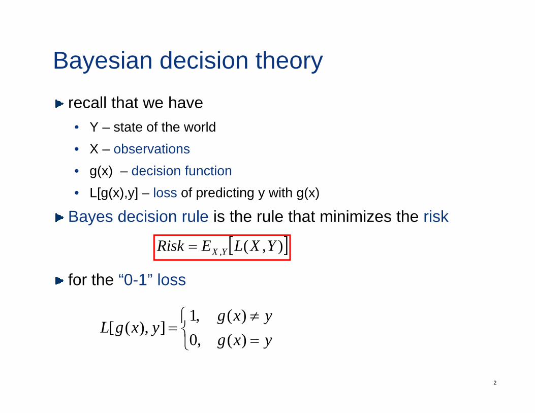
Bayesian decision theoryrecall that we have• Y – state of the worldY – state of the world• X – observations• g(x) – decision function• L[g(x),y] – loss of predicting y with g(x)

Bayes decision rule is the rule that minimizes the risk

for the “0-1” loss

[ ]),(, YXLERisk YX=

for the 0 1 loss

⎩⎨⎧ ≠

=yxg

yxgL)(0)(,1

]),([

2

⎩ = yxg )(,0

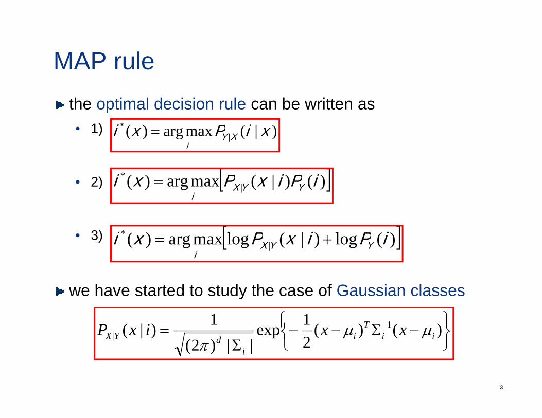
MAP rulethe optimal decision rule can be written as• 1) )|(maxarg)(* xiPxi1)

• 2)

)|(maxarg)( | xiPxi XYi

=

[ ])()|(maxarg)(* iPixPxi =• 2)

• 3)

[ ])()|(maxarg)( | iPixPxi YYXi

=

[ ])(l)|(l)(* iPixPxi +• 3)

we have started to study the case of Gaussian classes

[ ])(log)|(logmaxarg)( | iPixPxi YYXi

+=

we have started to study the case of Gaussian classes

⎭⎬⎫

⎩⎨⎧ −Σ−−

Σ= − )()(

21exp

||)2(1)|( 1

| iiT

idYX xxixP µµ

3

⎭⎩Σ 2||)2(|

idπ

The Gaussian classifierdi i i t

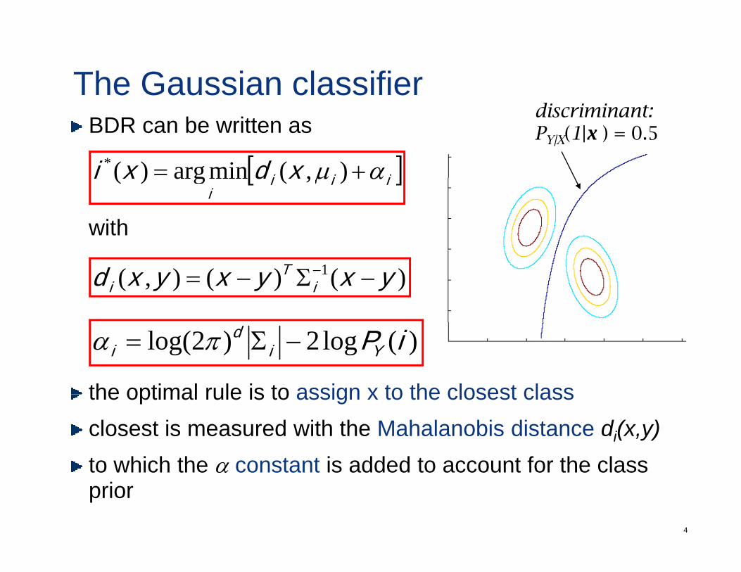
BDR can be written as

[ ]iii xdxi αµ += ),(minarg)(*

discriminant:PY|X(1|x ) = 0.5

with

[ ]iiii

xdxi αµ +),(minarg)(

)()(),( 1 yxyxyxd iT

i −Σ−= −

the optimal rule is to assign x to the closest class

)(log2)2log( iPYid

i −Σ= πα

the optimal rule is to assign x to the closest classclosest is measured with the Mahalanobis distance di(x,y)to which the α constant is added to account for the class

4

to which the α constant is added to account for the class prior

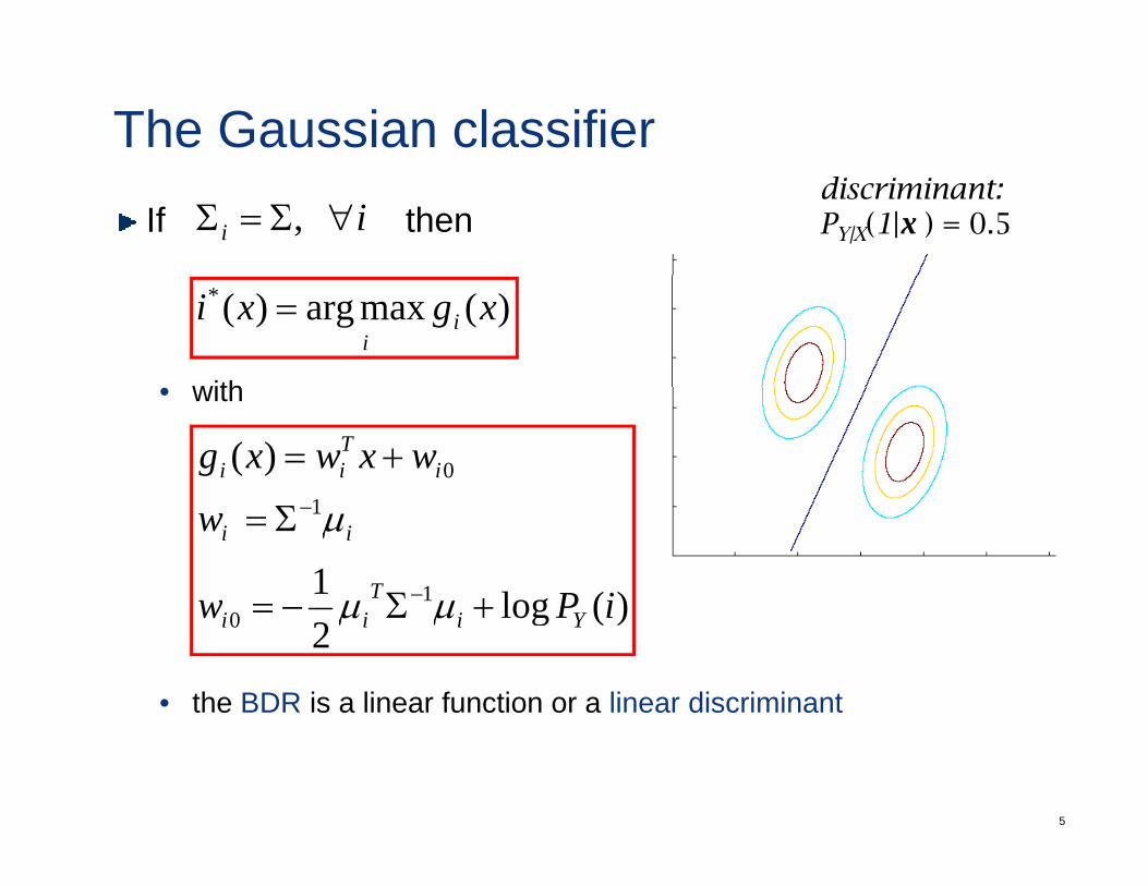
The Gaussian classifierIf then

discriminant:PY|X(1|x ) = 0.5ii ∀Σ=Σ ,

with

)(maxarg)(* xgxi ii

=

• with

)(1

0wxwxg iTii +=

)(log1 1

1

iPw

w

T

ii

+Σ−=

Σ=

−

−

µµ

µ

• the BDR is a linear function or a linear discriminant

)(log20 iPw Yiii +Σ= µµ

5

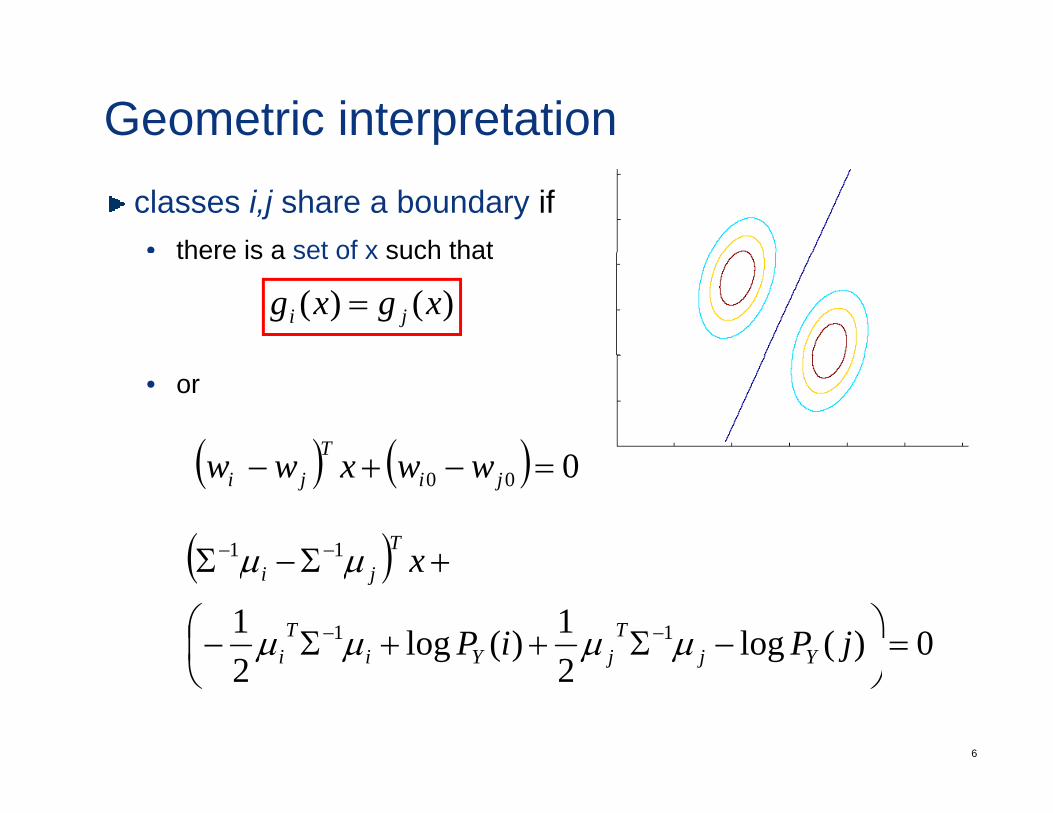
Geometric interpretationclasses i,j share a boundary if • there is a set of x such thatthere is a set of x such that

)()( xgxg ji =

• or

( ) ( ) 0T( ) ( ) 000 =−+− jiji wwxww

( )11 +ΣΣ −− xTµµ( )

0)(log21)(log

21 11 =

⎠⎞

⎜⎝⎛ −Σ++Σ−

+Σ−Σ

−− jPiP

x

YjT

jYiT

i

ji

µµµµ

µµ

6

22 ⎠⎝YjjYii

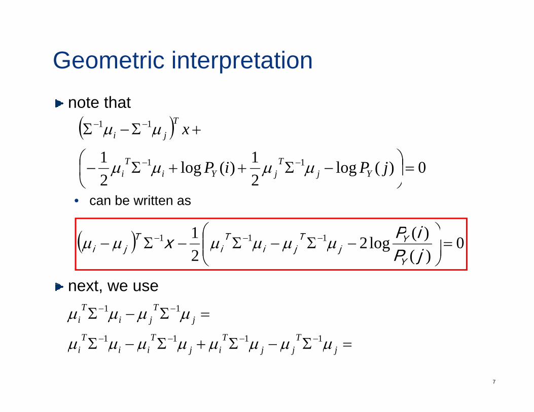
Geometric interpretationnote that( )11 +ΣΣ −− xT

µµ( )0)(log

21)(log

21 11 =⎟

⎠⎞

⎜⎝⎛ −Σ++Σ−

+Σ−Σ

−− jPiP

x

YjT

jYiT

i

ji

µµµµ

µµ

• can be written as

( ) )(1 ⎞⎛ iP

22 ⎠⎝

next we use

( ) 0)()(log2

21 111 =⎟

⎠

⎞⎜⎜⎝

⎛−Σ−Σ−Σ− −−−

jPiPx

Y

Yj

Tji

Ti

Tji µµµµµµ

next, we use

=Σ−Σ −−

TTTT

jT

jiT

i µµµµ1111

11

7

=Σ−Σ+Σ−Σ −−−−j

Tjj

Tij

Tii

Ti µµµµµµµµ 1111

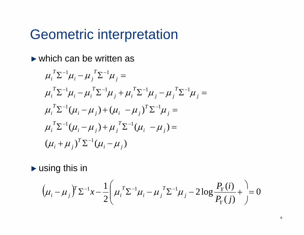
Geometric interpretationwhich can be written as

11 TT ΣΣ −−

1111

11

jT

jjT

ijT

iiT

i

jT

jiT

i

µµµµµµµµ

µµµµ

=Σ−Σ+Σ−Σ

=Σ−Σ−−−−

)()(

)()(11

11

jiT

jjiT

i

jT

jijiT

i

µµµµµµ

µµµµµµ

=−Σ+−Σ

=Σ−+−Σ−−

−−

)()( 1ji

Tji

jjj

µµµµ −Σ+ −

using this in

( ) 0)(log21 111 =⎞

⎜⎜⎛

+ΣΣΣ −−− iPx YTTT µµµµµµ

8

( ) 0)(

log22

=⎠

⎜⎜⎝

+−Σ−Σ−Σ−jP

xY

jjiiji µµµµµµ

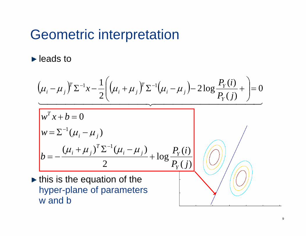
Geometric interpretationleads to

( ) ( ) ( )31

0)()(log2

21 11 =⎟⎟

⎠

⎞⎜⎜⎝

⎛+−−Σ+−Σ− −−

jPiPx

Y

Yji

Tji

Tji µµµµµµ

44444444444 344444444444 21

)(0

1wbxwT

−Σ=

=+− µµ

)()(log

2)()(

)(1

jPiPb

w

YjiT

ji

ji

+−Σ+

−=

Σ=− µµµµ

µµ

this is the equation of the hyper-plane of parameters

)(2 jPY

9

hyper plane of parametersw and b

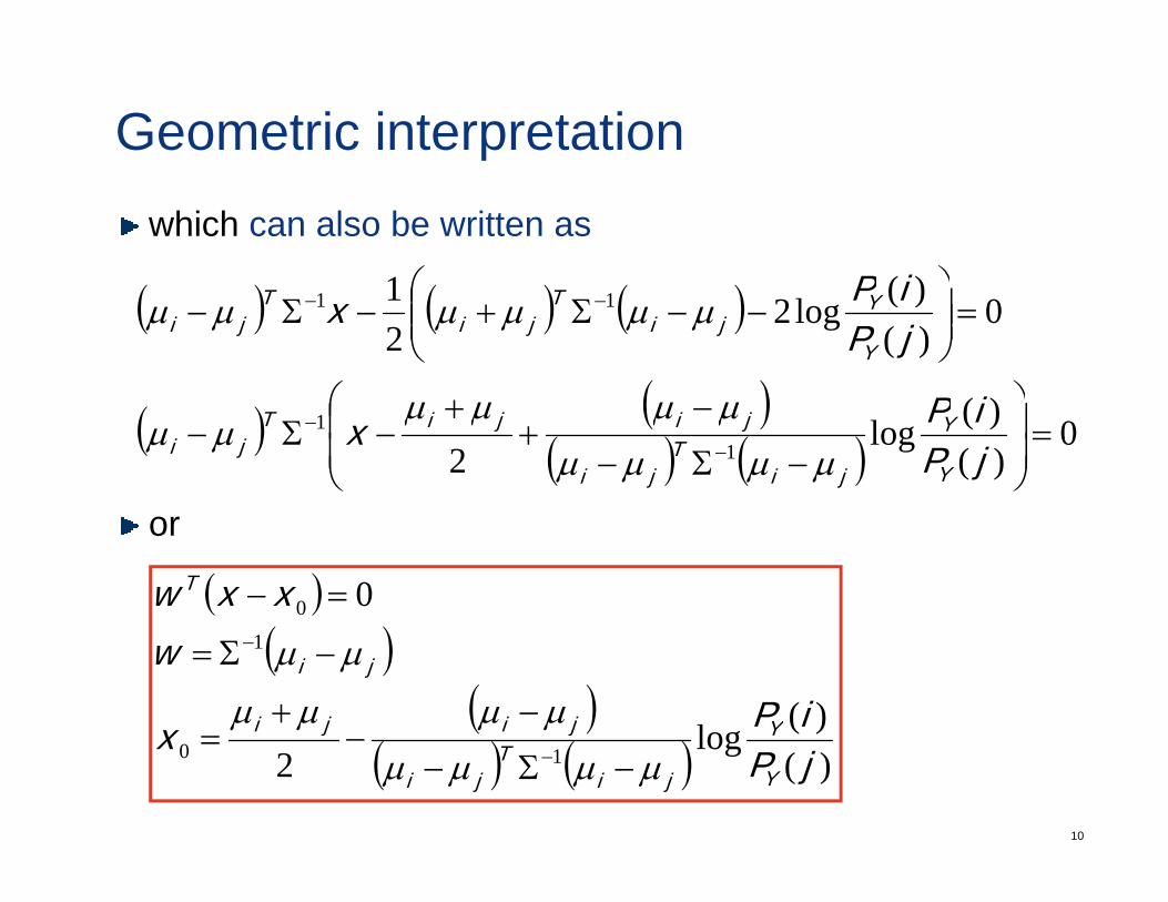
Geometric interpretationwhich can also be written as

)(1 ⎞⎛ iP( ) ( ) ( )

( )

0)()(log2

21 11

⎞⎛

=⎟⎟⎠

⎞⎜⎜⎝

⎛−−Σ+−Σ− −−

jPiPx

Y

Yji

Tji

Tji µµµµµµ

( ) ( )( ) ( ) 0

)()(log

2 11 =⎟

⎟⎠

⎞⎜⎜⎝

⎛

−Σ−

−+

+−Σ−

−−

jPiPx

Y

Y

jiT

ji

jijiTji µµµµ

µµµµµµ

or

( ) 00xxw T =−

( )( ) )(log

1

iPx

w

Yjiji

ji

µµµµ

µµ

−+

−Σ= −

10

( ) ( ) )(log

2 10 jPx

YjiT

ji µµµµ −Σ−−=

−

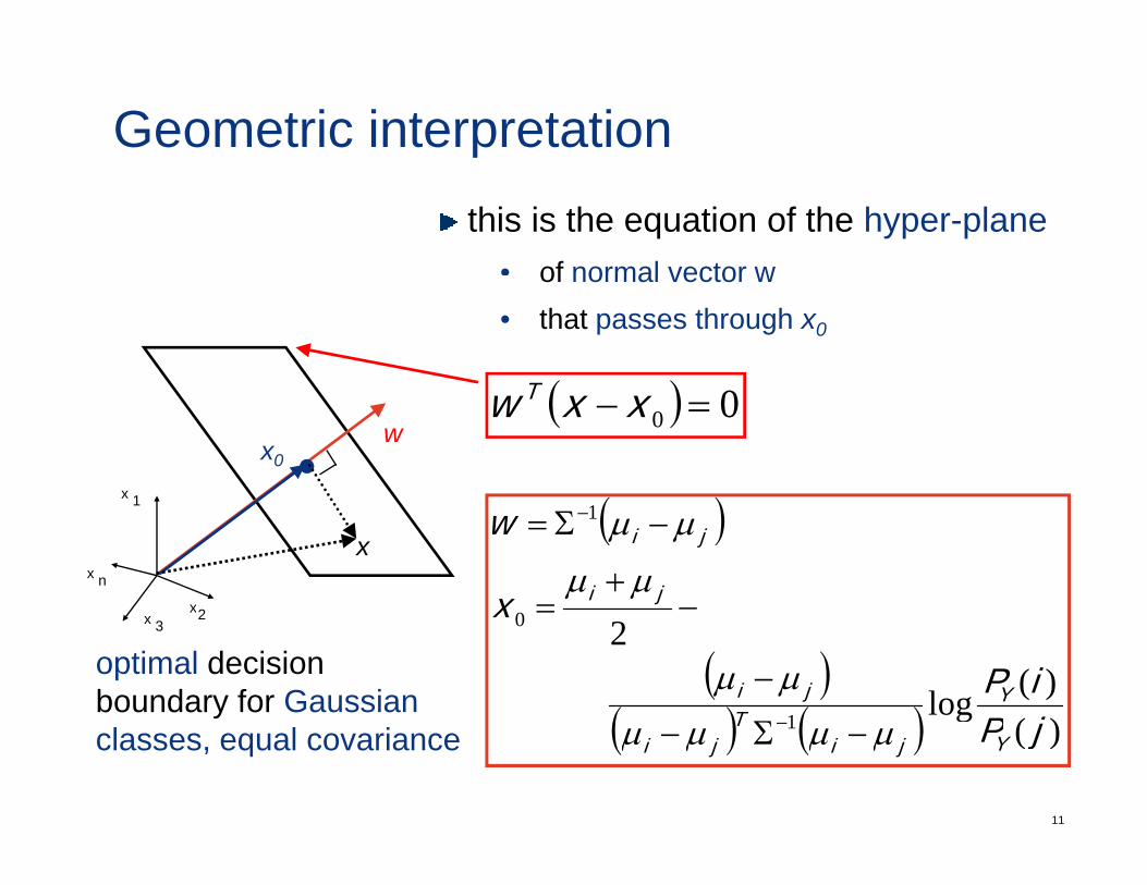
Geometric interpretationthis is the equation of the hyper-plane

• of normal vector wof normal vector w• that passes through x0

( )T ( ) 00 =− xxw T

x 1

wx0

( )1

x2

x n

x( )1

x

w

ji

ji

µµ

µµ

−+

=

−Σ= −

x 3x2

( )( ) ( ) )(

)(log

2

1

0

jPiP

x

YT

ji µµΣ

−

=

optimal decision boundary for Gaussian

11

( ) ( ) )(g

1 jPYjiT

ji µµµµ −Σ− −classes, equal covariance

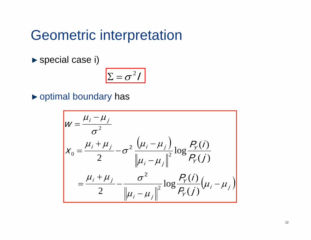
Geometric interpretationspecial case i)

I2Σ

optimal boundary has

I2σ=Σ

jiwσµµ −

= 2

( )Y

Y

ji

jiji

jPiPx

µµ

µµσ

µµ

−

−−

+=

)()(log

2 202

( )jiY

Y

ji

ji

j

jPiP µµ

µµ

σµµ−

−−

+=

)()(log

2 2

2

12

Yjijµµ )(

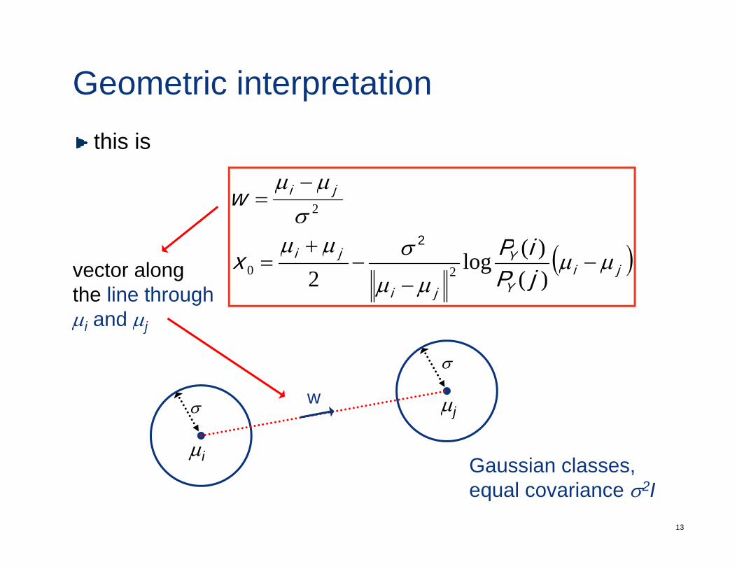
Geometric interpretationthis is

( )ji

ji

iP

w

σµµσµµ

+

−=

)(

2

2

( )jiY

Y

ji

ji

jPiPx µµ

µµ

σµµ−

−−

+=

)()(log

2 20vector alongthe line throughµ and µ

σ

µi and µj

w

µi

µjσ

Gaussian classes

13

Gaussian classes, equal covariance σ2I

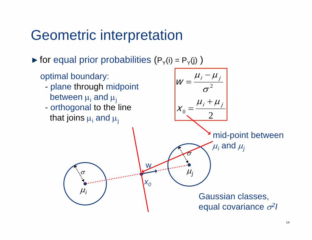
Geometric interpretationfor equal prior probabilities (PY(i) = PY(j) )

µµoptimal boundary:2

ji

jiw

µµσµµ

+

−=optimal boundary:

- plane through midpointbetween µi and µj

th l t th li20

jixµµ

=

mid point between

- orthogonal to the line that joins µi and µj

wσ

mid-point betweenµi and µj

w

µi

µjσx0

Gaussian classes

14

Gaussian classes, equal covariance σ2I

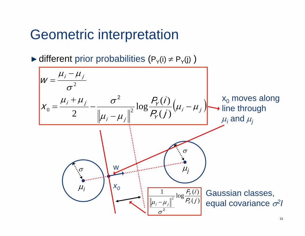
Geometric interpretationdifferent prior probabilities (PY(i) ≠ PY(j) )

µµ −

x0 moves along( )Yji

ji

iP

w

σµµσµµ

+

−=

)(l

2

2

line through µi and µj

( )jiY

Y

ji

ji

jPiPx µµ

µµ

σµµ−

−−=

)()(log

2 20

σ

w

µi

µjσ

x0Gaussian classes)(1 iPY

15

Gaussian classes, equal covariance σ2I)(

)(log12 jP

iP

Y

Y

ji2σµµ −

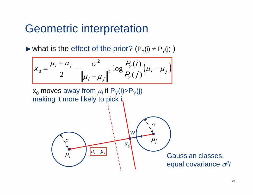
Geometric interpretationwhat is the effect of the prior? (PY(i) ≠ PY(j) )

iP2

( )jiY

Y

ji

ji

jPiPx µµ

µµ

σµµ−

−−

+=

)()(log

2 20

2

x0 moves away from µi if PY(i)>PY(j)making it more likely to pick i

wσ

µi

µjσx0

Gaussian classes, ji µµ −

16

equal covariance σ2I

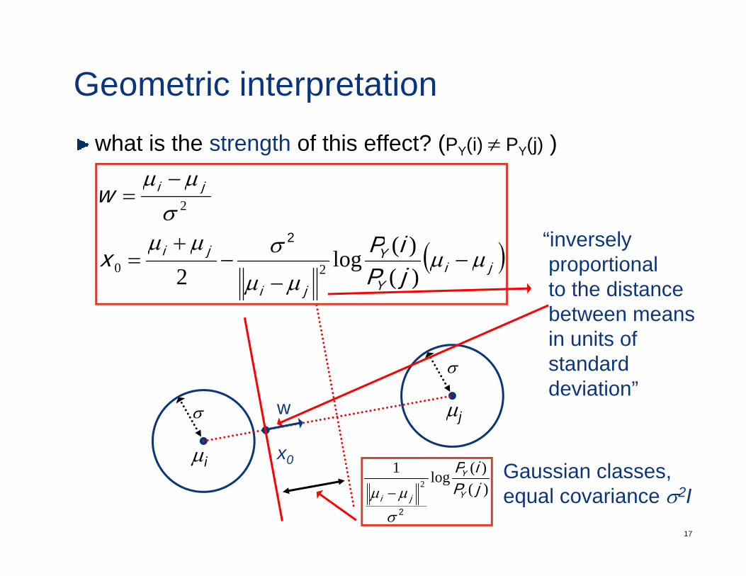
Geometric interpretationwhat is the strength of this effect? (PY(i) ≠ PY(j) )

µµ −

“inversely( )Yji

ji

iP

w

σµµσµµ

+

−=

)(l

2

2

proportionalto the distance between means

( )jiY

Y

ji

ji

jPiPx µµ

µµ

σµµ−

−−=

)()(log

2 20

σin units of standard deviation”

w

µi

µjσ

x0Gaussian classes)(1 iPY

17

Gaussian classes, equal covariance σ2I)(

)(log12 jP

iP

Y

Y

ji2σµµ −

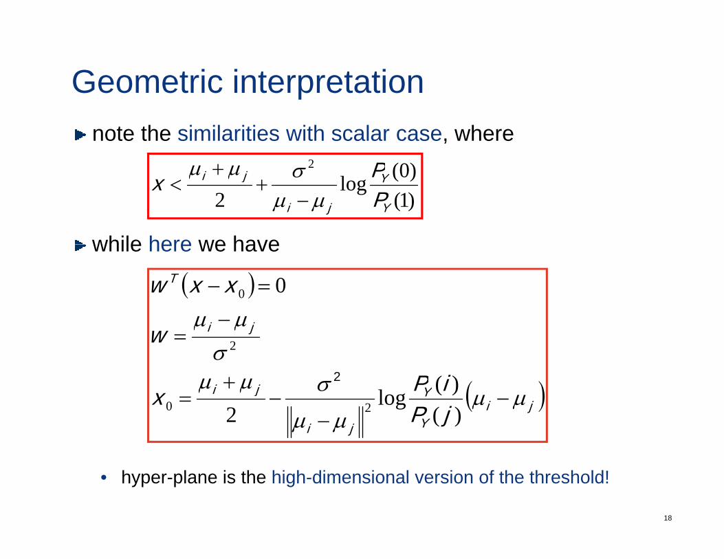
Geometric interpretationnote the similarities with scalar case, where

)0(2Yji Pσµµ +

while here we have

)1()0(log

2 Y

Y

ji

ji

PPx

µµσµµ−

++

<

while here we have

( )T xxw =− 00

( )ji

ji

iP

w

σµµσµµ

+

−=

)(

2

2

( )jiY

Y

ji

ji

jPiPx µµ

µµ

σµµ−

−−

+=

)()(log

2 20

18

• hyper-plane is the high-dimensional version of the threshold!

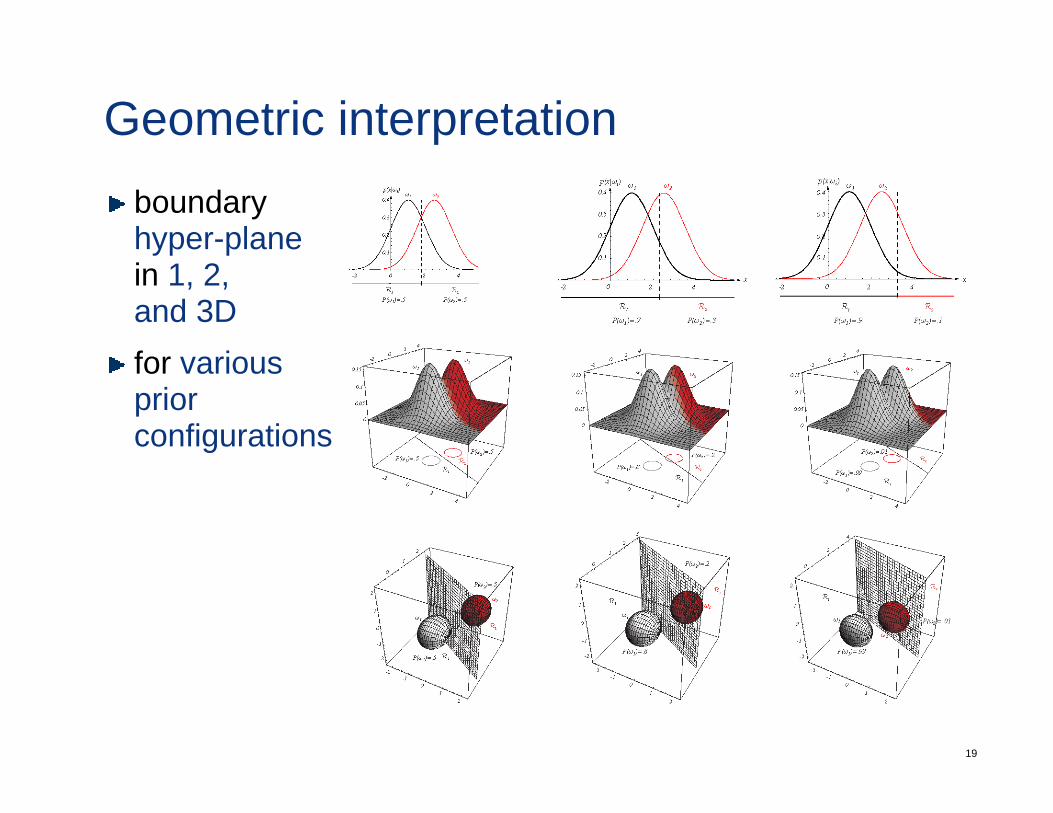
Geometric interpretationboundary hyper-planeyp pin 1, 2, and 3Df ifor various prior configurations

19

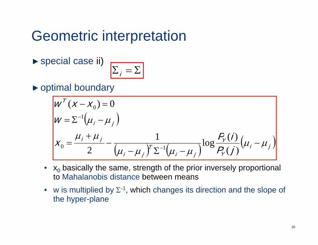
Geometric interpretationspecial case ii)

Σ=Σi

optimal boundaryT xxw =− 0)( 0

i

( )

( )Yji

ji

iP

wµµ

µµ

+

−Σ= −

)(1

)(1

0

• x0 basically the same strength of the prior inversely proportional

( ) ( ) ( )jiY

Y

jiT

ji

ji

jPiPx µµ

µµµµµµ

−−Σ−

−+

=− )(

)(log12 10

x0 basically the same, strength of the prior inversely proportional to Mahalanobis distance between means

• w is multiplied by Σ-1, which changes its direction and the slope of the hyper-plane

20

the hyper-plane

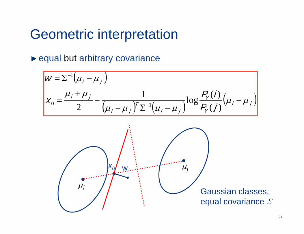
Geometric interpretationequal but arbitrary covariance

( )( )

( ) ( ) ( )jiY

Tji

ji

iPx

w

µµµµ

µµ

−−+

=

−Σ= −

)(log10

1

( ) ( ) ( )jiYji

Tji jP

x µµµµµµ −Σ− − )(

log2 10

w

µi

µjx0

Gaussian classes

21

Gaussian classes, equal covariance Σ

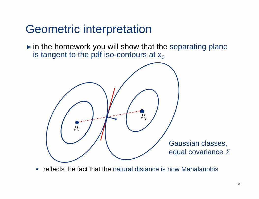
Geometric interpretationin the homework you will show that the separating plane is tangent to the pdf iso-contours at x0

µi

µj

Gaussian classes, equal covariance Σ

22

• reflects the fact that the natural distance is now Mahalanobis

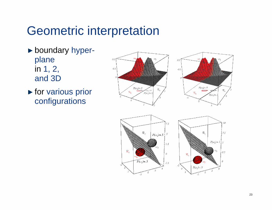
Geometric interpretationboundary hyper-planein 1, 2, and 3Dfor various priorfor various prior configurations

23

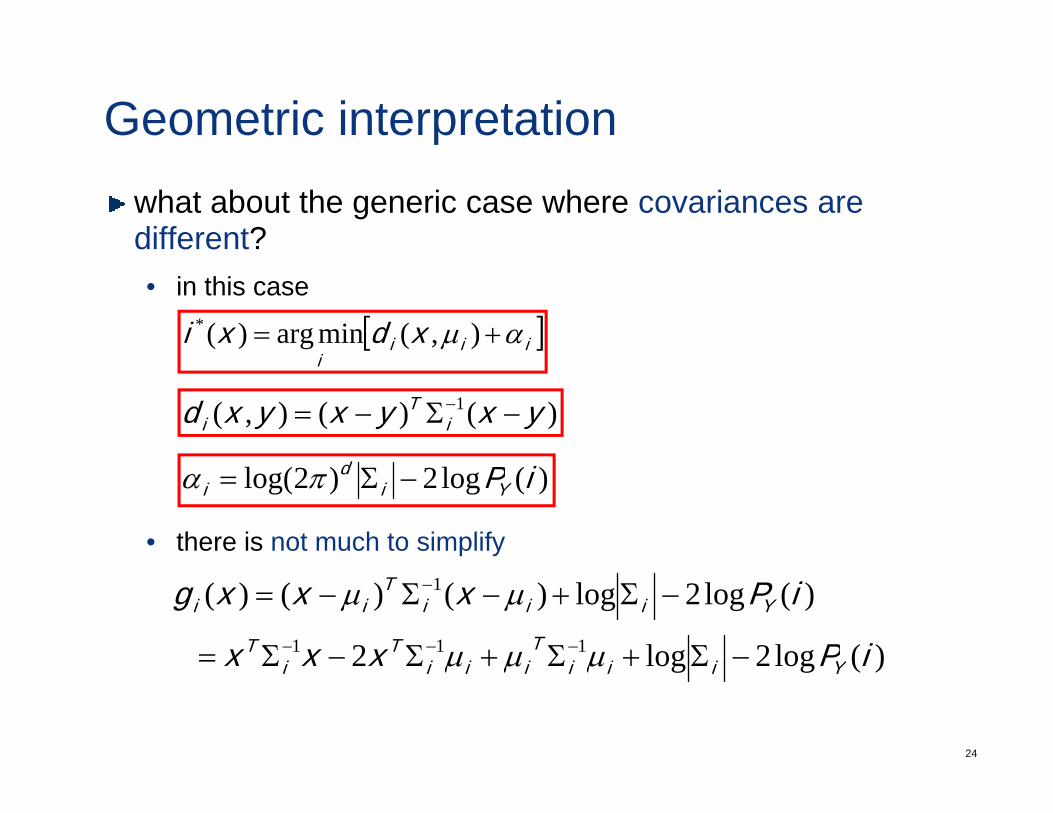
Geometric interpretationwhat about the generic case where covariances are different?• in this case

[ ]iiii

xdxi αµ += ),(minarg)(*

i

)()(),( 1 yxyxyxd iT

i −Σ−= −

• there is not much to simplify

)(log2)2log( iPYid

i −Σ= πα

)(log2log2

)(log2log)()()(111

1

iPxxx

iPxxxg

YiiiT

iiiT

iT

YiiiT

ii

−Σ+Σ+Σ−Σ=

−Σ+−Σ−=−−−

−

µµµ

µµ

24

)(log2log2 iPxxx Yiiiiiii Σ+Σ+ΣΣ µµµ

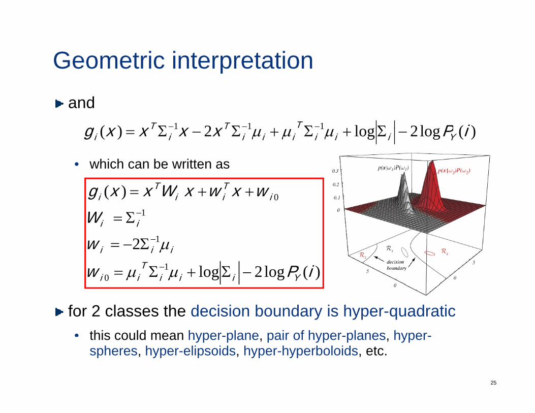
Geometric interpretationand

)(l2l2)( 111 iPxxxxg TTT Σ+Σ+ΣΣ −−−

• which can be written as

)(log2log2)( 111 iPxxxxg YiiiiiiT

iT

i −Σ+Σ+Σ−Σ= µµµ

)(1

0

W

wxwxWxxg

ii

iTii

Ti

Σ=

++=−

)(log2log

21

0

1

iPw

w

YiiiT

ii

iii

−Σ+Σ=

Σ−=−

−

µµ

µ

for 2 classes the decision boundary is hyper-quadratic• this could mean hyper-plane pair of hyper-planes hyper-

25

this could mean hyper-plane, pair of hyper-planes, hyper-spheres, hyper-elipsoids, hyper-hyperboloids, etc.

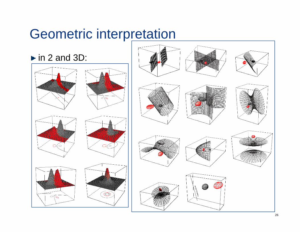
Geometric interpretationin 2 and 3D:

26

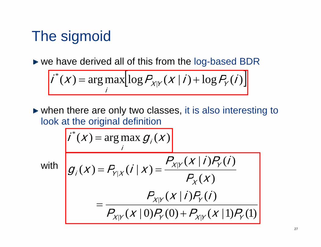
The sigmoidwe have derived all of this from the log-based BDR

[ ])(l)|(l)(* iPixPxi

h th l t l it i l i t ti t

[ ])(log)|(logmaxarg)( | iPixPxi YYXi

+=

when there are only two classes, it is also interesting to look at the original definition

)(maxarg)(* xgxi i=

with

)(maxarg)( xgxi ii

=

)()|()|()( | YYX iPixP

xiPxg ==

)()|()(

)|()(

|

|

YYX

XXYi

iPixPxP

xiPxg ==

27

)1()1|()0()0|()()|(

||

|

YYXYYX

YYX

PxPPxP +=

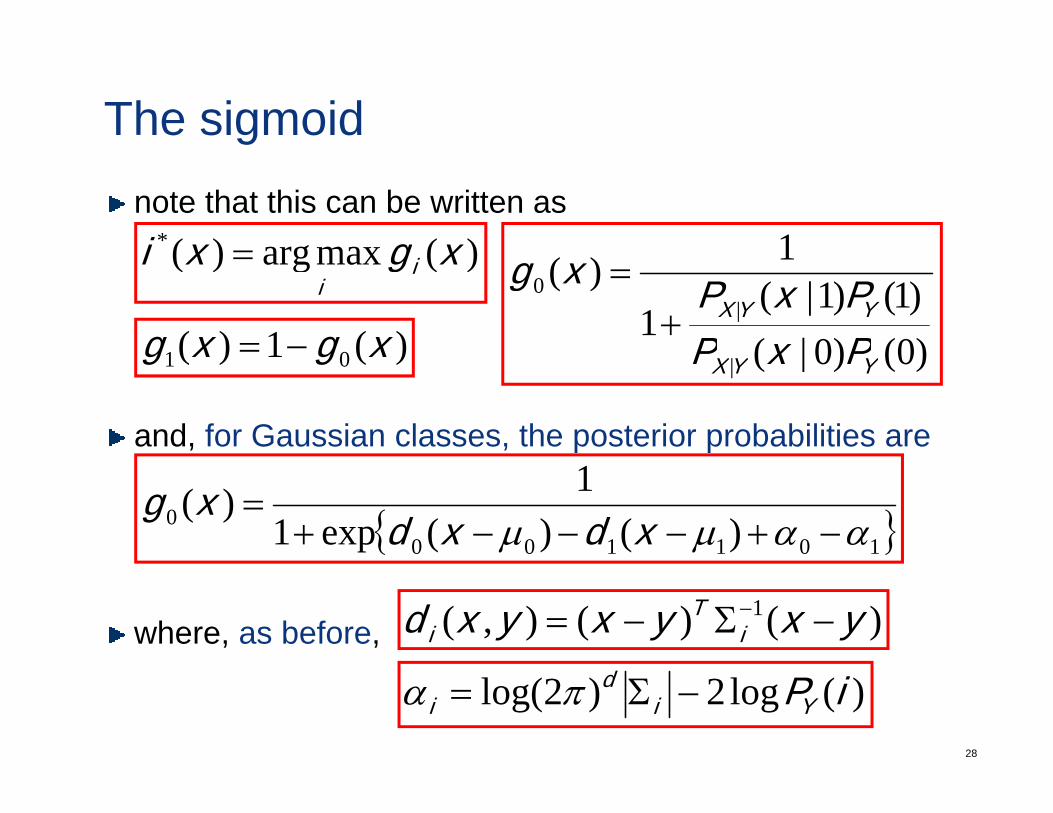
The sigmoidnote that this can be written as

)(maxarg)(* xgxi = 1)(maxarg)( xgxi ii

=

)0()0|()1()1|(

1

1)(|

0YYX

PxPPxPxg

+=

)(1)( 01 xgxg −=

and, for Gaussian classes, the posterior probabilities are

)0()0|(| YYX PxP)(1)( 01 xgxg

{ }1011000 )()(exp1

1)(ααµµ −+−−−+

=xdxd

xg

where, as before, )()(),( 1 yxyxyxd iT

i −Σ−= −

28

)(log2)2log( iPYid

i −Σ= πα

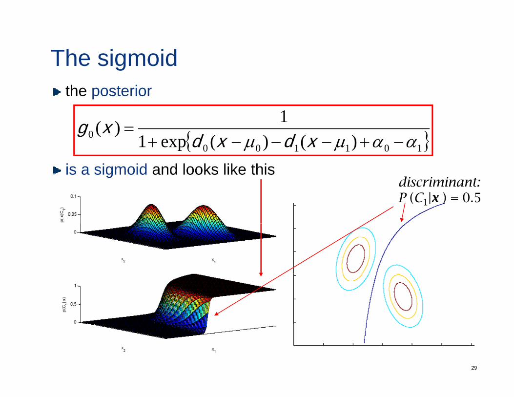
The sigmoidthe posterior

1)(g

is a sigmoid and looks like this

{ }1011000 )()(exp1

)(ααµµ −+−−−+

=xdxd

xg

is a sigmoid and looks like thisdiscriminant:P (C1|x ) = 0.5

29

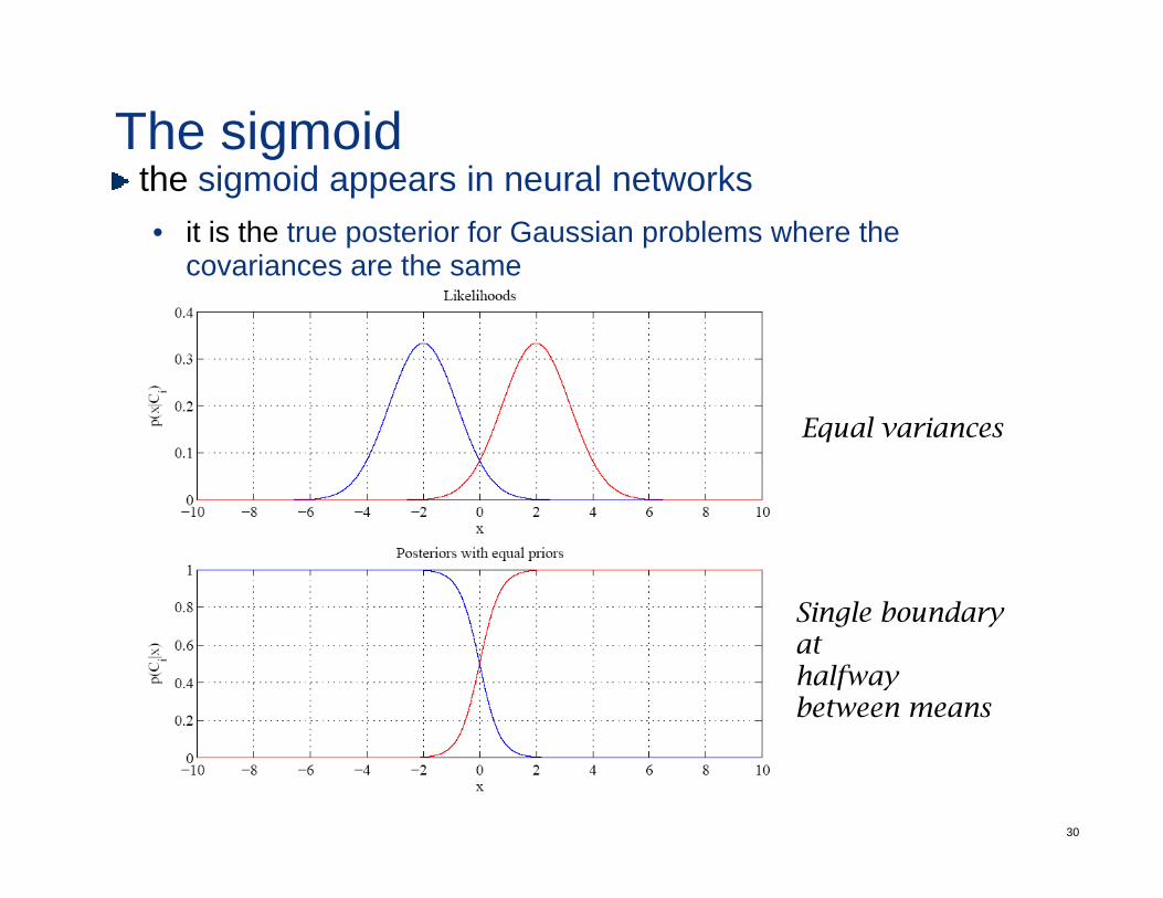
The sigmoidh i id i l kthe sigmoid appears in neural networks• it is the true posterior for Gaussian problems where the

covariances are the same

Equal variances

Single boundary Single boundary athalfway between means

30

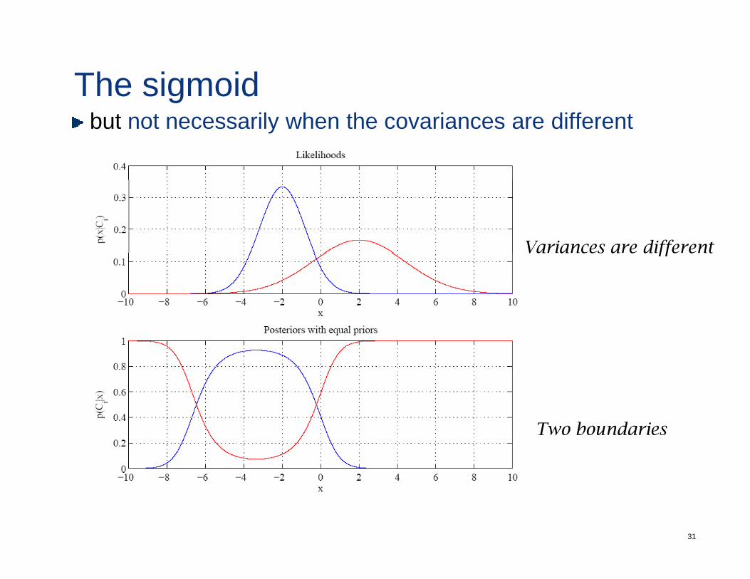
The sigmoidbut not necessarily when the covariances are different

Variances are differentVa a ces a e d ffe e t

Two boundaries

31

Bayesian decision theoryadvantages:• BDR is optimal and cannot be beatenBDR is optimal and cannot be beaten• Bayes keeps you honest• models reflect causal interpretation of the problem, this is how we

think• natural decomposition into “what we knew already” (prior) and

“what data tells us” (CCD)• no need for heuristics to combine these two sources of info• BDR is, almost invariably, intuitive

B l h i l d i li ti bl d l it• Bayes rule, chain rule, and marginalization enable modularity, and scalability to very complicated models and problems

problems:

32

p• BDR is optimal only insofar the models are correct.

33