The geographical information system QGis: a small guide to

The geographical information system QGis:a small guide to the practical exercises

Institute for Natural Resource Conservation Department of Hydrology and Water Resources Management

G. Hörmann

Mitarbeit: Ulrike Hanz (Session 1)Winter semester 2017/2018

Evaluierungscode WS17/18:

1 of 61 - D:\cloud\Dropbox\lehre\gis\qgis\qgis_tutorial_ws1718.odt -V2- 31/10/17 - 09:35:20

QGis-TutorialWS 2016/2017

Table of Contents

1 Introduction to QGIS.............................................................................................................................5

1.1 Starting QGIS..................................................................................................................................6

1.2 Projections.....................................................................................................................................6

1.3 Adding a layer................................................................................................................................7

1.4 Query and modify properties of the Map View and the data...............................................7

1.5 Query data (Attributes) from a Theme.....................................................................................8

1.6 Adding a first legend....................................................................................................................9

1.6.1 Changing legend colors and tables.................................................................................10

1.7 Overlaying different layers.......................................................................................................10

1.8 Creating maps from tables........................................................................................................11

1.9 Printing a View............................................................................................................................12

1.10 Display attributes as chart......................................................................................................12

1.11 Labelling a map.........................................................................................................................14

2 Editing and Analysis of Maps I..........................................................................................................16

2.1 Repetition 1..................................................................................................................................16

2.2 Repetition 2..................................................................................................................................16

2.3 Display information in table format.......................................................................................16

2.4 Joining tables (Join)....................................................................................................................17

2.5 Analysis of maps: calculation of a polygon area...................................................................19

2.6 Qgis Plugins..................................................................................................................................20

2.7 Group statistics............................................................................................................................20

2.8 Simple statistics..........................................................................................................................21

2.9 Simplifying a map and modification of values......................................................................22

3 Analysis and Editing of Maps II........................................................................................................25

3.1 Repetition.....................................................................................................................................25

3.2 Combining simple layers...........................................................................................................25

3.2.1 Creating new maps.............................................................................................................25

3.2.2 Combining simple elements.............................................................................................28

3.3 Merging and consolidating of polygons (“dissolve“)...........................................................29

3.4 Clipping maps with a mask (“clip“).........................................................................................30

3.5 Combining two maps (Operation „union“)............................................................................30



3.6 Creating Buffer Zones................................................................................................................31

4 Working with raster data..................................................................................................................33

4.1 Repetition.....................................................................................................................................33

4.2 File structure of raster maps in GIS.........................................................................................33

4.3 Working with raster files – first exercises.............................................................................34

4.4 Basic operations with DEMs......................................................................................................35

4.5 Using the Raster Calculator......................................................................................................38

4.6 Use of filters.................................................................................................................................39

5 Working with official DEMs..............................................................................................................41

6 Working with GPS data......................................................................................................................43

6.1 Repetition.....................................................................................................................................43

6.2 GPS introduction.........................................................................................................................43

6.3 Coordinate Systems....................................................................................................................43

6.4 Preconditions...............................................................................................................................44

6.4.1 Hardware..............................................................................................................................44

6.4.2 Digital Maps.........................................................................................................................44

6.4.2.1 Official sources...........................................................................................................45

6.4.2.2 Open source maps (open data)................................................................................45

6.5 Software........................................................................................................................................46

6.5.1 Software for mobile devices.............................................................................................46

6.5.2 GPS Software.......................................................................................................................47

6.5.3 Map Software......................................................................................................................48

6.6 Planning of a trip........................................................................................................................48

6.7 Things to consider during the trip..........................................................................................49

6.8 Retrieving the tracks..................................................................................................................50

6.9 Geotagging of pictures...............................................................................................................50

6.10 Display in Google Earth...........................................................................................................52

6.11 Modification and conversion of GPS tracks.........................................................................53

6.12 Analysis of gps tracks and integration in GIS......................................................................54

6.12.1 Integration of tracks and maps......................................................................................55

7 GIS in Hydrology.................................................................................................................................57

7.1 Flow direction and flow accumulation...................................................................................57

7.2 Hydrological catchments..........................................................................................................58

7.3 Calculation of a stream network..............................................................................................58



8 Formal requirements for the protocol............................................................................................59



1 Introduction to QGISQGIS is a user friendly Open Source Geographic Information System (GIS) licensed under the

GNU General Public License. QGIS is an official project of the Open Source Geospatial

Foundation (OSGeo). It runs on Linux, Unix, Mac OSX, Windows and Android and supports

numerous vector, raster, and database formats and functionalities. (www.qgis.org)

QGIS always exists in two versions: a so called “long term support” (LTS, actually 2.18)

version and “normal” version (actually 2.18). The aim of the LTS version is to provide

commercial users with a stable version for a long time, usually about 2-6 years. The

software development continues during this time, new versions with new features are

published regularly. In addition there are also beta versions, these are not recommended

for work.

Organisational issues

The files for each individual session can be found on OLAT and in the following

directory: Y:\austausch_kurs\gis choose subfolder with session-ID.

1. You will find more subfolders in the folder carrying the session-ID, e.g. shapes, grids. Copy the content of this directory to your local work directory or to your personal network drive at the beginning of each session!

2. Example: The files for session 1 can be found in Y:\austausch_kurs\gis\session1. There is a subfolder named shapes. Copy this folder to a local drive e.g. c:\practical_gis\

Do not work directly on network drives, you have no write access rights and you will not be able to save your work

If you work with the zip-archives from OLAT you have to extract all files. If you only double-click the archive, you open files directly inthe archive and QGIS will not find all files.

1.1 Starting QGIS➢ Open the program from the Windows Program Manager (Start Programs QGIS

QGIS Desktop (or more recent Version))


http://www.qgis.org/


GIS vocabulary

Project A file containing references to all files related to the current work

task. The Project is the central container of your current work.

Map A window for viewing GIS data.

Layer A layer is an in-memory file that references and displays data which

is stored on disk

GroupLayer Like a folder where related Layers can be combined. Layers can be

dragged-and-dropped as well as copied and pasted into and from

Group Layers

QGIS starts with an empty project.

➢ Save project as session1.qgs to make sure that your work won´t get lost at the end of

the session.

Now we will go into detail. The first aim is to become familiar with the graphical user

interface (GUI). QGIS provides menus at the top of the window, which show a panel of

actions. Now we will add data and get some information on the maps afterward.

1.2 ProjectionsQGIS displays maps of the curved earth surface on a plane. Similar to any hardcopy map

projections are used for this purpose. We use the Universal Transverse Mercator-projection

(UTM). When starting a new project, the proper projection should be defined in “Settings”-

“Options” and the “CRS”. In the section choose “Default CRS for new projects” choose “

EPSG: 4326-WGS 84”. You can also choose the measurements units in the section “Map

tools”-“Measure tool”- “Preferred measurements unit”.



1.3 Adding a layer QGIS allows maps to be composed of raster (dot matrix data structure) or vector (points,

lines, curves, and shapes or polygons) layers. On the left side there a numerous buttons to

add different layers to your map. Here we will use a vector layer.

ArcMap vocabulary

Shapefile A file which contains spatial data (polygons, lines, points)

“.dbf”- file which contains attributes in the dBase format

“.shx” - Indexfile

Select “Add vector layer”-“Source”-“Browse” and choose “C:\session1\landuse.shp”

Ticking the small box in the left part of the “Layers” in front of “landuse”, the map of

landuse (dis-) appears.

1.4 Query and modify properties of the Map View and the data

➢ Select “Layer”- “Properties…” and choose in “Style”-“Color” a different background

color. Confirm with “OK”.


Figure 1: The main windows of QGis


➢ Right-click the layer “landuse” in the layer section directly and go to “Properties”

choose the section “General”-“Layer Info” and rename the layer to Land Use 1.

1.5 Query data (Attributes) from a ThemeGIS vocabulary

Attributes Properties which are attributed to the objects of a layer. Attributes

are organised in tables with each table row representing an

individual object.

Overview of Attributes

➢ Right click the layer in the Layer section and choose “Open Attribute Table”

➢ A table with several columns appears. Information is given about the type of object,

its identification (ID) and an additional property (Gridcode). Gridcode is the


Figure 2: Adding a vector layer


attribute carrying the land use information, each number stands for a specific land

use type. The number of rows is equivalent to the number of layer´s polygons.

Query Attributes directly from the Theme

➢ Click on “Identify Features” then right click an object on the map in order to get the

ID.

Highlight objects in the Theme

➢ Click on “Select Feature by area or single click” then click on an object on the

map. The polygon and the respective row I the Attribute table are marked in blue or

yellow color.

Show objects selected in the Attribute Table in the Theme

➢ Right click the layer in the Layer section and choose “Open Attribute Table”

➢ Left-click the grey box in a row (use the shift key to select multiple objects)- the

selected object(s)is/are marked yellow in the map, Many objects are too small to be

seen, then click on “Zoom map to the selected rows” in the section above.

➢ Zoom in with or double click

➢ Zoom out with or

➢ Move section with

➢ Show complete map

➢ Zoom to selection

➢ Zoom to previous/next extent

1.6 Adding a frst legendFor now your map is a little bit boring because all land use classes are drawn with a uniform

symbol. We will assign a unique color to each class.

➢ Double-click the layer in the Layer section or right click and choose “Properties”.

➢ Choose the tab “Style”, then “Categorize” and then the Column “Gridcode” and click

“Classify” and then “OK”

➢ Set the desired color ramp

➢ The map has a new legend with a unique color for each gridcode



Figure 3 Adding a legend to the map

1.6.1 Changing legend colors and tables

➢ Go to “Layer Properties”, “Style” and Double click on the entry in the “Legend”

section, define a new label text

➢ A double click on a colored box opens a menu with additional options for color etc.

1.7 Overlaying diferent layersOne strength of the concept of the map is that multiple layers can be presented at the same

time. In the following we will learn more about the potential of this tool.

Click

➢ Select the file riv1.shp .This layer contains lines as objects (a river network)

➢ Repeat the last step with outlet1.shp – now we see a layer with points (runoff

gauges)

Some tips for working with multiple Themes

➢ The order of the layers can be changed by moving the layer in the layer section with

the mouse up or down.

➢ The display of the layer can be deleted by right-click the layer and choose “Remove”

➢ Multiple layers can be selected by clicking holding the shift key

➢ A layer is (de)activated by clicking on the box shown in Fig. 4. This click only

changes the display of the file, it is not removed from the project.



➢ “related” Layers can be combined in group layers. Therefor click (Add group)

Layers can be dragged and dropped into and out of group layers

1.8 Creating maps from tablesSpatial information is not only stored in maps, but also in tables from databases or

spreadsheets, e.g. the position of experimental plots or routing information. In QGIS you

can create maps from these tables. In this exercise we will create a map from a table with

spatial information about the position of meterological stations in the Treene catchment. In

contrast to ArcGIS there is no way to import a .dbf file directly. Therefor you have to change

the .dbf file into a .csv file.

➢ Click (Add Delimited Text Layer) and open treene_wetterstat.csv, set

custom delimiters and choose the X-/Y-Values in the table and remove the tick from

DMS Coordinates press OK.

➢ Change the size of the symbols to make them more visible.


Figure 4: (De)activation of a layer


Figure 5 Adding a .csv file as a layer

1.9 Printing a View ➢ You can save the view with Project → Save as Image in many different filetypes

and print it or

➢ Choose Project → New Print Composer

➢ A new window will open, on the left side you can add all elements you want to add

➢ Add new label to add a title

➢ Format the scale of the map (1:50,000)

➢ Add a reasonable size of the scalebar

➢ Add a north arrow and change it

➢ Change the presentation such as only land use is shown in the composer

➢ Add a map to the layout

➢ Export the layer in a good quality for including it in reports or documents

1.10 Display attributes as chartA common application is the display of spatial statistics, e.g. the areal fraction of land use.

➢ Create a new project



➢ Open the map county_borders

➢ Select Properties → Diagrams

➢ Move the fields you want to be drawn to the right side, press OK

Figure 6 Display attributes as charts- creation of charts

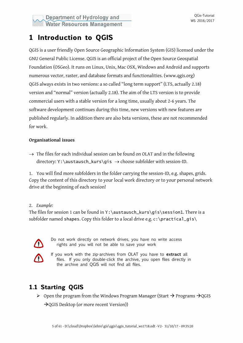
If you want to display values as histograms you have to check the scale (see Fig. 7). Sometime the bars are not displayed because the scale is set not set at all or set to the wrong scale.



1.11 Labelling a mapFrequently we need some sort of text in a map. A typical example is the name of a city or

country. Fig. 6 shows how to get labels in maps.

➢ Select Properties → Labels, tick the box “Label this layer with” and select

the field Kreisname

➢ Modify text color or other properties if needed


Figure 7: Options for histograms/barcharts


Figure 8 Labelling features in a map

Figure 9 Combination of labels and charts



2 Editing and Analysis of Maps I

Please copy the folders of this session from y:\austausch_kurs\gis or from OLAT to your local work directory.

2.1 Repetition 1Create a new project. Add the maps riv1.shp (the river network) and outlet1.shp (the position of the gauges) to this view. Use this view to create a layout which shows only

the section of the View which includes the river network

the gauges of type “T” (without deleting anything!). What is the location of the gauge nearest to the outlet of the catchment?

2.2 Repetition 2A very common task in GIS is to plot variables in a map. A typical example is the distribution of nutrient contents on an agricultural field, yields of different farms etc. A typical example for this type of data is the Meuse data set1 from http://spatial-

analyst.net/book/meusegrids. It contains the location and contents of heavy metals in the soil near the river Meuse.

• Load the shape file with the data set and plot the contents of heavy metals as a chart in the map

2.3 Display information in table formatIt is also possible to load tables without spatial information. In our case this is a table with the names of the land use classes – in the map we only find the numeric codes in field gridcode. The screen shot in fig. 10 shows the most important options.

1 Rikken, M.G.J. and Van Rijn, R.P.G., 1993. Soil pollution with heavy metals –- an inquiry into spatial

variation, cost of mapping and the risk evaluation of copper, cadmium, lead and zinc in the oodplains of

the meuse west of Stein. Utrecht: Department of Physical Geography, Utrecht University.



• Select “Create a layer from delimited text file”

• Select the file luc.dbf, mark the options as shown in fig. 10. The option 'no geometry' is important, if you do not select it, Qgis thinks that this file contains spatial coordinates.

2.4 Joining tables (Join)Create a layer with the name landuse from the first exercise. Unfortunately, the map does not contain the names of the land use classes, only the numeric code. These names and the numeric code are save in the luc data base we added in the last chapter. Now, we link the two tables together – this is called a join in data base language. It is used e.g. to assign the names of the land use classes to the gridcodes.

• Load the landuse2 map from last session

• Right-click on landuse and select Properties → Joins (see fig. 11)

• Select the join layer luc (the data base with the names)

• Select the fields in the two data bases which contain the numeric code, value and gridcode.

• Click OK and take a look at the attribute table, it now contains the names of the landuse classes.

You can now change the legend of landuse_new to display the names of the landuse class, not only the numerical code.


Figure 10: Importing a data table


The tables are not physically changed (i.e. the files are not modified), Qgis only saves the logical link between the two tables. If you want to make it permanent, open the attribute table.

1. The join operation only works for identical data type of the columns, i.e. you cannot join numbers and text, even if the text variable contains a number.

Now let us start with the analysis of maps. First we want to calculate the distribution of the different land use classes.

2.5 Analysis of maps: calculation of a polygon areaThe calculation of an area and other geometric properties is quite easy.

• enter edit mode and write the function in the appropriate field (Fig. 12)


Figure 11: Joining two data bases


In the following chapters you can find several methods to calculate the fraction of the different land use classes

2.6 Qgis PluginsSome features are not part of the base version of Qgis, but have to be installed as plugins. Installation is quite ease: just select the plugin from the list and click on install. The plugin


Figure 12: Calculation of a polygon area – quick and dirty solution

Figure 13: Calculation of an area with field calculator


we need for the analysis of data bases is called Group Stats. It contains functions similar to Pivot tables in spreadsheets.

2.7 Group statistics Group statistics are a common in data analysis, in spreadsheets they are called pivot table. Atypical group question for our data base would be: what area is covered by the different land use classes?

➢ Select Vector → Group Stats → Group stats

➢ Select the layer you want to analyse, the columns and the rows. The entries marked in Fig. 15 calculate a table with total area (sum) for each GRIDCODE.

➢ if you want to plot or analyse the results, you can export the table to a file or to the clipboard.


Figure 14: Plugins in QGis


2.8 Simple statistics


Figure 15: Summarizing a data set

Figure 16: Simple statistics


If you only need an overview of a column you can also use the icon shown in fig. 16 and select layer and column. The same results are calculated by the plugin Statist and by selecting Vector → Analysis Tools → Basic Statistics.

2.9 Simplifying a map and modifcation of valuesIf you get maps from other sources, frequently the codes do not match your needs: the satellite map has 30 different land use classes, but your model knows only about 4. In the following steps we want to simplify the map and merge the codes of some land use classes which are very similar. The fields FRSD and FRSE are merged into the common class “forest”, RNGE, RNGB und PAST are merged into “grassland”. The solution for this task is a modification of the attribute table.

➢ Open landuse.shp and open the attribute table.

➢ Start editing (left icon in fig. 17)

➢ Add a new field, name it and define a data type (fig. 17)

The recoding procedure is composed of two steps: first, select the records and second recode the new field.


Figure 17: Add a field to a attribute table


➢ use “select by expression”, enter the condition (fig. 18) and click on select.

The records are now selected

➢ Enter the new code with the short (fig. 19) or long version of the field calculator

➢ If you need to select more than one value you can use the different select commands

(fig. 20) or add logical conditions to the select menu.


Figure 18: Select GRIDCODE=1 in the data base

Figure 19: Assign a new value to the new field


LANDUSE LAND_LONG Old Value New ValueAGRL Agricultural Land 1 1RNGB Rangeland (Brush) 2 2RNGE Rangeland (Grass) 3 2URBN Urban 4 4WATR Water 5 5FRSD Deciduous Forest 6 6FRSE Evergreen Forest 7 6PAST Pasture 8 2

➢ In the next step, we will change the old values 2 and 3 to the new value 2, i.e. we need two selections. You can carry out these functions separately, but it is easier to use the database functions in the select window directly. Here you can add, select and remove from the current selection – in database language this stands for an OR or and AND condition (fig. 20). In our case we

o select the gridcode = 2 and then

o Add to selection” for gridcode = 3. Now, all values with 2 or 3 are marked. Right click on the column code_new and select Field Calculator.Carry out the calculation with code_new = 2. Now, all records with Gridcode=2 and 3 have code_new = 2.

➢ Repeat the two steps for all codes from the table above.

We have now reduced the number of classes and can draw a new legend.

➢ Modify the table luc.dbf and adjust it to the new codes

o


Figure 20: Options for a selection


3 Analysis and Editing of Maps II

3.1 Repetition• Use the Meuse data set from Session 2

i TCalculate the deviation from the mean value of Cd concentrations in %

i TPlot the results as spatial chart

3.2 Combining simple layersIt is difficult to understand what happens if you combine two maps with the different tools available. To facilitate this process a little bit, we created two very simple layers and watch how the resulting map and the data base look like after the operation.

3.2.1 Creating new maps

First, we create a new, empty layer (fig. 21) Layer → Create Layer → New Shapefile Layer. The type of the layer is “polygon”.

If you want to draw different figures like rectangles, circles etc. you have to use the plugin “Rectangles Ovals Digitizing” (Fig. 23).

Start Editing and select the newly generated layer (fig. 22).

You can use the Sketch Tool to draw a few geometrical forms in the view. Right click when you have reached the final point to finish, and choose a name for the polygon.


Figure 21: creating a new layer


Because we need two maps, we create a second layer. This time we draw some circles directly on the map as graphics (the plugin has to be installed).

Now click on the attribute table of the two maps and add some explanatory text in both columns, the Name field and the FROM1 and FROM1, e.g. From1P0


Figure 22: Drawing a rectangle

Figure 23: Drawing geometric elements with the plugin Rectangles Ovals Digitizing



Figure 25: Combining simple elements

Figure 24: Drawing elements in a map


3.2.2 Combining simple elements

You can load the circle and rectangle maps from the session directory and apply the different functions.

If something goes wrong and the result is not what you expected you should check the geometry of the map in Vector → Geometry. In case of more problems you can use the v.clean function from the GRASS system.

First, try the Vector → Geoprocessing → Dissolve function and check the visual results and the attribute table.

the clip function cuts out parts of a map.

Next, try the intersect function and check the visual results and the attribute table.

Next, try the Union function and note the empty fields of the attribute table!

And finally we use the merge function


Figure 26: Geoprocessing functions


Note how the fields are combined

3.3 Merging and consolidating of polygons (“dissolve“)Many polygons of our land use map are situated next to other polygons with the same land use. Now we want to simplify our map and merge all polygons with the same land use into one single polygon. This also increases the speed of all spatial operations like e.g. the calculation of area from the last session.

➢ Add the reclassified land use map from session 2 (landuse2.shp) with an appropriate legend. Join table luc_own.dbf to the map.

➢ Select Vector → Geoprocessing Tools → Dissolve and select Code_New or gridcode as the dissolve field (fig. 27).

ArcMap Vocabulary

Dissolve Merge polygons with the same attribute

➢ You should also recalculate the fields like Area.

If records of the attribute table are selected, only these records are used for the operation, not the complete map.

3.4 Clipping maps with a mask (“clip“)Up to now, we have always used the entire map for our calculations. In real life however we use mostly only a part of a map, e.g. one single catchment. This partial map is created with aclipping operation.


Figure 27: Dissolving the landuse map


ArcMap Vocabulary

Clip Clip one layer based on the mask of a second layer.

➢ Use the dissolved landuse map and add the map of the catchment ezg.shp.

➢ Vector → Geoprocessing Tools → Geoprocessing → Clip

➢ Select Input Features → landuse2_dissolve_c and Clip Features ->ezg. Name the Output Feature Class → landuse2_Dissolve_clip and confirm with OK.

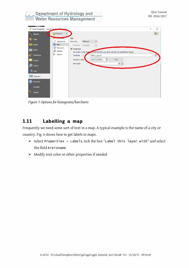
3.5 Combining two maps (Operation „union“)If two layers with different information (attributes) are needed for an analysis, we have to combine the two layers in one layer. Because the polygons of two different layers are rarely equal it is not possible to simply copy the attribute table (as in the join operation), but the polygons have to be recalculated with all attributes. As an example, we want to combine theland use and the soil map of our catchment.


Figure 28: Clipping land use of the catchment area


➢ use the file from the last paragraph landuse2_dissolved_clipped and add soil_treene.

➢ Vector → Geoprocessing Tools → Geoprocessing → Union (Fig. 29)

GIS Vocabulary of characteristic map combination tools

Union Join two themes with different polygons

Intersect Attributes of the common area of two themes are joined; similar to

Union, but can also contain line and point elements.

Merge The attributes of two themes are merged together, but not as a

permanent intersection but a simple addition of the polygons. It is

therefore possible that there are several polygons from theme B

hidden behind a polygon of theme A. With operation Intersect

the polygons would be visible.

Erase Cut out a part of the map (similar to the cut)

i Calculate the area with agricultural land use on soil type GG-SS (Gley-Subtype) in union_landuse_soil.shp

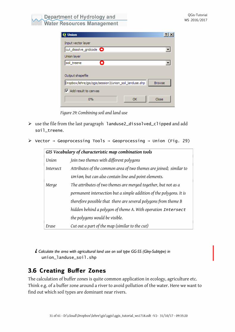
3.6 Creating Bufer ZonesThe calculation of buffer zones is quite common application in ecology, agriculture etc. Think e.g. of a buffer zone around a river to avoid pollution of the water. Here we want to find out which soil types are dominant near rivers.


Figure 29: Combining soil and land use


Add riv1.shp layer to the map

Vector → Geoprocessing Tools → Geoprocessing → Buffer and calculate a buffer around the rivers with 500m width.

i Use the methods you learned before to calculate the distribution of the soils in the buffer zone

around the rivers. The result should be a table or a chart.

o


Figure 30: Buffering a river


4 Working with raster data

4.1 RepetitionOur task is to find suitable locations for windmills. We will use three criteria to test the suitability:

wind speed must be higher than 4.3 m/s (M50>9), locations with lower wind speed are not suitable

Urban areas (1), landfills (9) and mining areas (8) should be avoided

the locations must not be protected by laws for nature conservation. The status of the locations is coded as:

o unsuitable locations: NR (nature reserve, 2), planned NR (future nature reserve, 5), natural park protection area (1),

o partly suitable: natural park (6), landscape conservation area (LCA, 3), planned LCA (4)

o suitable locations: all other locations

Load the maps land_use.shp, protection.shp and wind.shp. Use these maps to create amap with suitable locations for windmills by combining the different maps.

If you code the suitability with numbers 0/1/2, the final calculation can be done by multiplying the suitability of the different maps. There are at least 3 different ways to create the final map.



To speed things up, you should dissolve as much as possible before joining the maps.

4.2 File structure of raster maps in GISA raster map is stored in two folders: Grid and Info. These folders are called “Workspace” and may not be separated or deleted.

GIS Vocabulary

Workspace Container of all files and directories of a raster map.

4.3 Working with raster fles – frst exercises

➢ import thunderhead_mountain_tn.dem (a part of the digital elevation model of Tennessee (http://63.148.169.50/dem.html, date of access: 07.12.04, Website no longer available)


Figure 31: Importing a DEM file

http://63.148.169.50/dem.html


You can also change the legend to singleband pseudocolor (Fig. 32), change the number of classes or adjust colour schemes (Fig. 32). It is also possible to change single colours by clicking on the colour symbol.

The following chapter shows some basic operations with a digital elevation model (DEM).

4.4 Basic operations with DEMs New ArcMap Vocabulary

Contours Contour lines (e.g. Elevation).

Slope Vertical Slope (measured in ArcMap in degrees)

Aspect Exposition (given as direction north/south)

Hillshade Reflexion of the surface with a imaginary illumination

Viewshed Visible part of the site from a virtual viewpoint


Figure 32: Changing the display of a DEM


Always use the original DEM as a base file. It does not make sense to calculate the aspect of the slope

• Calculate slope, aspect and hillshade. Some interesting examples of shading can be found at http://www.reliefshading.com.

• Create contour lines: Raster → Extraction → Contour

A common application of raster analysis is the “viewshed” analysis. The viewshed is what you see if you stand on the top of a mountain. In Qgis this function is handled by a plugin called Viewshed analysis.


Figure 33: Common operations with raster files

http://www.reliefshading.com/


• Create a point layer with points with the position of the viewers (preferably located somewhere on the mountain top).

• Select the eye-icon and fill out all options to calculate viewshed (Fig. 34).


Figure 34: Options for viewpoint analysis


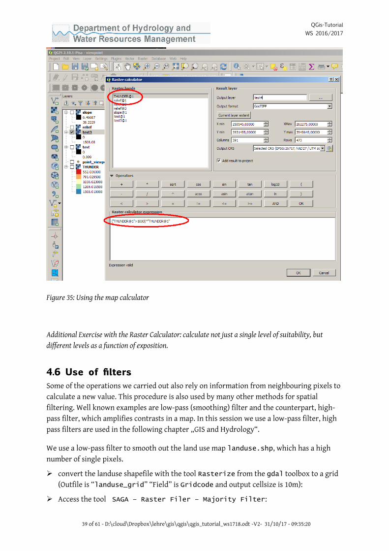
4.5 Using the Raster CalculatorUp to now we have loaded grids directly or we have created them by single commands based on information contained in the file. However, we often need a combination of different areas, e.g. to test an area for suitability of a planned land use. In this situation, we can utilize the so called Raster → Raster Calculator. We use it now to answer the following question about our grid thead:

„Which areas of Thunderhead Mountain lie below a defined elevation (e.g. 1000 m), are oriented towards the south and have a slope below 10°. These parameters define the suitability of a region to grow grapes for wine (we disregard here some minor other factors for viticulture like the frequency of fast food restaurants in the region 8-)

To answer this question we merge different maps with the following operations carried out with the raster calculator:

• Open the Raster Calculator, see Fig. 35

• create a query like e.g. ([Aspect of thead_grid] >= #Value#) and ([Aspect of thead_grid] <= #Value#) and ([Slope of thead_grid] < #Value#) and ([Thead_grid] < #Value#).



Additional Exercise with the Raster Calculator: calculate not just a single level of suitability, but different levels as a function of exposition.

4.6 Use of flters Some of the operations we carried out also rely on information from neighbouring pixels to calculate a new value. This procedure is also used by many other methods for spatial filtering. Well known examples are low-pass (smoothing) filter and the counterpart, high-pass filter, which amplifies contrasts in a map. In this session we use a low-pass filter, high pass filters are used in the following chapter „GIS and Hydrology“.

We use a low-pass filter to smooth out the land use map landuse.shp, which has a high number of single pixels.

➢ convert the landuse shapefile with the tool Rasterize from the gdal toolbox to a grid (Outfile is “landuse_grid” “Field” is Gridcode and output cellsize is 10m):

➢ Access the tool SAGA – Raster Filer – Majority Filter:


Figure 35: Using the map calculator


o This filter assigns the value of a pixel to the most frequent pixel in the neighbourhood. We define number of neighbours as „Eight“ and replacement threshold as „Majority“ („a clear majority needs to be obtained” – scientific statement can found in the help file).

➢ The Map Calculator is also quite useful if we want to compare the results of different filter operations.

➢ Calculate the difference between landuse_grid and landuse_majflt with Raster -> Raster Calculator, the result is a map with the differences due to the filter operation.

Code für Evaluierung: CUWNW

Adresse: http://studfeedback.uni-kiel.de/evasys/indexstud.php

o



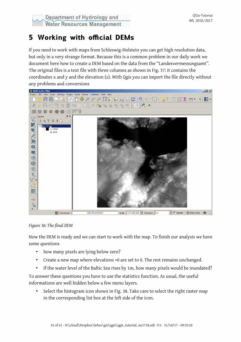
5 Working with official DEMsIf you need to work with maps from Schleswig-Holstein you can get high resolution data, but only in a very strange format. Because this is a common problem in our daily work we document here how to create a DEM based on the data from the “Landesvermessungsamt”. The original files is a text file with three columns as shown in Fig. 37: it contains the coordinates x and y and the elevation (z). With Qgis you can import the file directly withoutany problems and conversions

Now the DEM is ready and we can start to work with the map. To finish our analysis we havesome questions

• how many pixels are lying below zero?

• Create a new map where elevations <0 are set to 0. The rest remains unchanged.

• If the water level of the Baltic Sea rises by 1m, how many pixels would be inundated?

To answer these questions you have to use the statistics function. As usual, the useful informations are well hidden below a few menu layers.

• Select the histogram icon shown in Fig. 38. Take care to select the right raster map in the corresponding list box at the left side of the icon.


Figure 36: The final DEM



Figure 37: Format of the raw data file

Figure 38: The final DEM

Figure 38: Histogram of a DEM


6 Working with GPS data

6.1 RepetitionIn the directory bundestagswahl you can find a map with the German election districts (“Wahlkreise”) and the results of the elections for the Bundestag 2009. Create the following maps:

• Map of all election districts in Schleswig-Holstein

• A map with the election results of all different parties (pie-charts) for first and second votes (Erst- und Zweitstimme)

• A map with the percentage of votes for the Green party, the CDU and the SPD (Zweitstimmen), the percentage should be coded as color.

6.2 GPS introductionA few years ago, mapping with GPS was a kind of black art with expensive equipment. Today, GPS chips are integrated in nearly all electronic devices from computers to watches. However, for most people GPS is a separate application and they do not use it together with a GIS.

This chapter is based on the work flow you use to plan a trip – be it your Sunday afternoon walk or a botanic excursion to Siberia.

GPS vocabulary

Waypoint: A single point in a landscape (e.g. location of sampling, normally marked

with some explanatory text like “station 1”)

Track: A number of points recorded continuously by a GPS device, e.g. the path of a

walk. During a sampling campaign the locations can be assigned by

comparison of the time. The same procedure is used for

Photo tagging: Assigning a location to a picture by comparing the time stamps of a

GPS track and the time recorded by the camera in the so called EXIF

properties.

6.3 Coordinate SystemsThe Universal Transverse Mercator (UTM) geographic coordinate system uses a 2-dimensional Cartesian coordinate system to give locations on the surface of the Earth. It is ahorizontal position representation, i.e. it is used to identify locations on the Earth



independently of vertical position, but differs from the traditional method of latitude and longitude in several respects.

The UTM system is not a single map projection. The system instead divides the Earth into sixty zones, each a six-degree band of longitude, and uses a secant transverse Mercator projection in each zone (wikipedia.org).

The administrative building of Kiel University (Verwaltungshochhaus) has the following different coordinates:

ETRS89/UTM zone 32N, geogr. coordinates 572938.21E 6021755.34N

ETRS89/UTM, Lat/Lon Decimal (32U), WGS84 54.33870lat 10.121860lon

Gauss Krüger, 3. Meridian 3573075 (Rechtswert,

Easting)

6023773 (Hochwert,

Northing)

For a comparison of the different coordinates for North-Germany see http://portal.digitaleratlasnord.de/

6.4 Preconditions

6.4.1 Hardware

There are basically two different groups of devices to register your position: mobile phones and specialised devices, e.g. from Garmin.

Mobile smartphones are cheap and very flexible. There are a lot of programs for navigation, gps logging, geocaching etc. For Android mobiles we can recommend the program “gps Logger” or the OSM logging software. If you also want to plan your trips with your mobile, apemaps (http://www.apemap.de/) and komoot (www.komoot.de) are good choices. Both programs are also able to log your trip and they are especially suitable for biking and trekking.

Garmin navigation systems are less flexible and sometimes artificially limited in their functions. The only real advantage is that the batteries last much longer than those of the mobiles. If you plan to purchase one of these devices make sure that you can use the maps from Open Streetmap (www.openstreetmap.de) – the commercial maps from Garmin are much more expensive, but not better. The professional gps devices (e.g. Leica) are a completely different story: the precision is directly related to the price.

6.4.2 Digital Maps

The maps you need for gps are quite different from scientific maps – they mostly include the common maps you use for orientation. Unfortunately, many maps do not come free but must be purchased. As usual, there is also an open source alternative to the expensive commercial products.


http://www.openstreetmap.de/




6.4.2.1 Official sources

Official sources of maps include commercial maps and governmental (official) maps. Examples for commercial maps are the Mapsource packages (http://www.magicmaps.de, often linked to Garmin GPS), but also the official topographic maps.

If you need maps for education and/or research in Schleswig-Holstein, you can get official data at Kiel University from [email protected].

6.4.2.2 Open source maps (open data)


Figure 39: OpenStreetMap of the university campus (screenshot from an Android

mobile)


The best maps you can actually find for trekking and biking are the maps from the Open Street Map (OSM, http://www.openstreetmap.de/) project. OSM maps actually have more details than Google Maps. If you take a close look at the screenshot in Fig. 39 you can see that even the nearly inofficial footpaths are mapped (red arrows in the figure).

OSM maps can also be used in Garmin devices instead of the expensive Garmin Software.

6.5 Software

6.5.1 Software for mobile devices

For your mobile device you need at least a so called GPS-Logger, a program which saves your position in a file while you are on the way. Many navigation programs like komoot or the OSM software have already a built-in logger. If you use the OSM-software and work in a remote, unmapped area you can help to build a map of this region.

Fig. 40 shows a screenshot of a common GPS program (GPS status) on an Android mobile.



6.5.2 GPS Software

The most important format in the GPS world is the gpx format from Garmin. Other important formats are the KML format from Google earth and – naturally – the different GISformats like shp.

One of the most useful programs for general conversions is the freeware G7towin. You can use it to transfer files from/to your device and to convert the tracks to KML format.

If you use your mobile to take your pictures, you can save the gps coordinates directly in the EXIF-part of your pictures. For pictures from a normal camera you can use geotagging programs like e.g. geosetter. Both programs use the time as key. The position of a picture is attributed to the gps position at the same time. All geotagging programs can deal with time differences between cameras and the GPS device.


Figure 40: Screenshot of a GPS Logger (Android)


6.5.3 Map Software

GIS software is not very well suited to plan your field trips. A better choice is a software which can communicate with your GPS-device or at least produce files for download. The following packages are a good choice:

• Google Earth (can communicate directly with Garmin GPS in both directions)

• Komoot (online version and mobile version available). Combines planning and tracking in one package, automatic syncing of tracks between desktop PC and mobile

• apemap (windows version, same as komoot, but comes with Windows software, works with OSM maps)

6.6 Planning of a tripIf you want to avoid unpleasant surprises during a walk, you better plan your trip before you start. A few years ago, you used a hiking/trekking map and you made a raw estimation of the distance. Today, you can use a digital map, plan your trip on screen, download the track of your plan to your GPS. If you use software like komoot, the planned trips are synchronised between your home PC and your mobile device. Whatever software you use, the basic procedure remains the same:

• trace your trip on your PC with a digital map. For many well known tracks you can download official tracks from the tourist information websites.

• Save the track in GPX-format on your PC

• download the track to your mobile device or use Dropbox to sync your files.

Fig. 41 Shows the two main windows of the komoot software. The advantage of this solutionis that all files all synced automatically between your PC and your mobile device. If you want, you can also share your trips on the website with everyone.



i use the website www.komoot.de to create a walk near your birthplace (or whereever you want

to go). Check the precision of the different map displays.

6.7 Things to consider during the tripDuring the trip the use of the software is quite straightforward.

Always carry a least one spare battery with you. Current mobiles only last a few hours with one charge, i.e. your device goes offline after the lunch break. Garmin devices last 1-3 days with one set of batteries.

Switch on logging before you start. By default, the gps logging is deactivated to avoid drain of the battery.

On Garmin devices, do not save your track if you want to use time stamps later for foto tagging. Saving deletes the time stamp.

If you want to georeference your pictures after the trip, take a picture of the gps display. This helps you to correct the time deviations between camera and gps.


Figure 41: Navigation (left) and logging window (right) of the komoot program

http://www.komoot.de/


6.8 Retrieving the tracksThere are several methods to retrieve your tracks after a trip

• some programs (komoot e.g.) sync automatically all tracks between your mobile andyour computer

• you can use a service like dropbox to sync your tracks manually if your tracker does not support automatic syncing.

• Many GARMIN devices are able to link to a PC with an USB cable and mount a drive where you can find your tracks.

• Read data from your GPS, e.g. with the free programs g7towin (http://www.gpsinformation.org/ronh/) or EasyGPS (http://www.easygps.com/). Google Earth is also able to link directly to a GPS

Usually, all files come in the gpx-format. If not you can use g7towin to convert to/from most other formats.

6.9 Geotagging of picturesA common gps application is the georeferencing or geotagging of pictures. E.g. if you are mapping land use or animals you can store the coordinates in the picture for later display on maps. In Fig. 42 you can see the geosetter program. It uses the time stamp of the gps track and of the image and adds the position to the image meta-information, i.e. the EXIF part, where all technical information is saved.

Most image viewers can display this information. In Fig. 43 we used the open source image

viewer Irfanview to display the EXIF information. If you want you can call Google Earth

directly from IrfanView and check the position of the image.

• Geotag the pictures in the pictures directory with geosetter

• select Images Open Folder→

• select Synchronize with GPS Data files




Figure 42: Screen of the geosetter program

Figure 43: Display of GPS information with IrfanView


6.10 Display in Google Earth

As a first try it is a good idea to display the tracks in Google Earth. You can load gpx-tracks directly as shown in Fig. 44. In Fig. 45 you can see that there can always occur some errors: some parts of the track are located directly on the lake – and even older scientists can not walk on the water. It is not clear if the problem is the track or the image. However, the trackon the bridge is very precise.

i Oload the track in google earth, check the precision visually (e.g. near rivers)


Figure 44: Display of a GPX-track in Google Earth


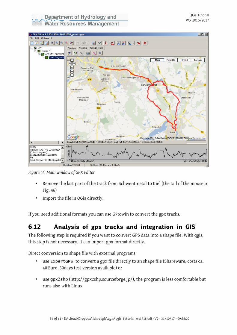
6.11 Modifcation and conversion of GPS tracksSometimes it is necessary to simplify or modify the GPS tracks of your trip. We recommend the program GPX_Editor.exe for this tasks – it runs from any directory and does not need an installation.

• Load the file preetz.gpx


Figure 45: Errors displayed in Google Earth


• Remove the last part of the track from Schwentinetal to Kiel (the tail of the mouse inFig. 46)

• Import the file in QGis directly.

If you need additional formats you can use G7towin to convert the gpx tracks.

6.12 Analysis of gps tracks and integration in GISThe following step is required if you want to convert GPS data into a shape file. With qgis, this step is not necessary, it can import gpx format directly.

Direct conversion to shape file with external programs

• use ExpertGPS to convert a gpx file directly to an shape file (Shareware, costs ca. 40 Euro, 30days test version available) or

• use gpx2shp (http://gpx2shp.sourceforge.jp/), the program is less comfortable but runs also with Linux.


Figure 46: Main window of GPX Editor


99% of the problems related to the import of GPS data are caused by wrong

projections - a nightmare even for experienced GIS users. Check also the format of

your coordinates (UTM, Gauss-Krüger, decimal format of h/min/sec format) and the

decimal separator (comma, point).

6.12.1 Integration of tracks and maps

If you plot GPS tracks you normally want to show them based on a regular map. A good choice for base maps openstreetmap.org. You can download these maps free of charge e.g. for most countries from http://downloads.cloudmade.com/, but you can also do it in QGIS directly.

First, you have the choice of different plugins:

• the plugin GPS-Tools offers a comfortable way to communicate with GPS devices.

• both plugins, OpenLayers or QuickMapServices can download background maps.

The import of a track is quite simple:

• activate GPX-Tools

• click on the GPX-icon and import the file (Fig. 47)

• You can also import any gpx file as a regular vector layer (Fig. 48)

The import of a background map is quite easy:


Figure 47: Import of a gpx track with GPS-Tools

http://downloads.cloudmade.com/

http://downloads.cloudmade.com/


• activate one of the Plugins (QuickMapServices or Openlayers) and import the selected map (Fig. 49)

• if the track is not visible you have to move it to the top of the display.

• Load the track kairouan_clean.gpx and check the quality of the different background maps.

o


Figure 48: Direct import of a gpx file

Figure 49: Adding an OpenStreetMap Layer to the track


7 GIS in Hydrology

In the last session, we have shown you the functions for spatial analyses. A common application for DEMs is the calculation of hydrologic properties like e.g. flow direction or the delineation of hydrologic catchments. In this session we will use some standard procedures which are mostly based on functions of the TauDem Toolbox. The same functions are available from the GRASS toolbox. Unfortunately, both, the TAUDEM toolbox


Figure 50: The Hydrology Toolbox


and the Grass system are a little bit ricky to set up. Please check the processing options in Fig. 51. More information is available from the website:

http://hydrology.usu.edu/taudem/taudem5/downloads5.0.html


http://hydrology.usu.edu/taudem/taudem5/downloads5.0.html


7.1 Flow direction and fow accumulation In this session we work with the file thunderhead.

• For the calculation of flow direction we first need to eliminate undrained sinks (abflusslose Senken). Undrained sinks are mostly not a natural element of the landscape (except for Schleswig-Holstein) but an artefact caused by errors in the DEM. This is why they are normally deleted i.e. (virtually) filled up with the tool “Pit Remove”.

• Use the Raster Calculator to compare the filled up DEM with the original.

• We continue our work with the filled DEM and create a raster map of the flow direction with D8 Flow Direction. Use the filled DEM as input! The direction of the actual pixel is set to the direction with the greatest slope to the neighbouring cells. It is coded as: E = 1, SE = 2, S = 4, SW = 8, W = 16, NW = 32, N = 64, NE = 128.


Figure 51: Setup parameters for the TauDEM toolbox


• The flow accumulation is a function of the flow direction grid, it is calculated with Flow Accumulation. The resulting number is the number of pixels which drain into the actual pixel.

7.2 Hydrological catchments • Catchments are separated by divides. These divides are points where the flow

accumulation is equal to zero (0). First we copy the themes Filled thead_grid and Flow Accumulation to a separate group layer named “Watershed” and use the Raster Calculator to find these pixels.

• The resulting picture has many pixels which match the search. The reason for this rather diffuse picture is that we did not define a minimum area for our catchment. Every small hill/valley is now acting as a hydrological divide.

• This problem can be solved with the tool “Basin”, we use the flow direction raster.

• As a result we get a raster containing the watersheds – not very useful for our catchment in Schleswig-Holstein.

7.3 Calculation of a stream networkTo derive a stream network to locate rivers we need to follow this procedure:

• Use the Raster Calculator to distinguish between cells that are assessed as being a stream and cells that are considered being part of overland flow areas. (select the cells of the flow accumulation grid that are larger than a threshold, e.g. 180)

• Use the tool “Stream to Feature” from the Hydrology toolbox to convert the obtained raster to a shapefile.

• Repeat the calculations for the raw DEM (without fill), compare the resulting river network with official data in fliessgewaesser.shp.

o



8 Formal requirements for the protocolYour solutions of the problems should be documented in a protocol which has to be delivered at the Department of Hydrology by 15st of February 2016.

The layout, structure and level of detail should follow the customs and the format required for a scientific paper. The protocol should explain your proceedings in solving the tasks in a comprehensible manner, but there is no need to explain all mouse clicks in detail. Also include the required tables, maps and calculation results.

● Your results and conclusions must be traceable for a student/scientist with a

reasonable understanding of GIS.

● Figures have captions below the image, all text should be readable.

● Tables with caption above

● A caption should comprise a brief title (not on the figure itself) and a description of

the illustration or table. Keep text in the illustrations themselves to a minimum but

explain all symbols and abbreviations used

● Figures and tables should be discussed/referred to in the text near the location of

their display.

● no fancy formatting: no text floating around figures and table

● use paragraph and character templates, no manual formatting of headers etc. !

● Page limit: between 5 and max. 10 pages

You can submit the text by email or on CD-ROM. I will send a short confirmation messagefor each submission by email. If you do not receive this confirmation, your text has not arrived and somehow disappeared in the deep waters of the internet or was killed by aspam-filter.

o


Documents

The geographical information system QGis: a small guide to