The geometry of EPR correlations

The geometry of EPR correlations

Otfried GuhneAna C.S. Costa, H. Chau Nguyen, H. Viet Nguyen, Roope Uola

Department Physik, Universitat Siegen

Overview

1 Motivation: Entanglement and steering

2 Steering criteria from entropic uncertainty relations

3 Two-qubit steering: Geometric approach

4 Two-qubit steering: Practical calculation

5 Conclusion

Steering

Bell inequalities

Alice and Bob share a state |ψ〉.

Bell inequalities

Alice and Bob measure Ax and By , obtain the results a, b.

Question: Can the probabilities be written as

P(a, b|x , y)?=∑λ

pλp(a|x , λ)p(b|y , λ)

Bell inequalities


Bell inequalities

Alice and Bob measure Ax and By , obtain the results a, b.

Question: Can the probabilities be written as

P(a, b|x , y)?=∑λ

pλp(a|x , λ)p(b|y , λ)

Entanglement


Entanglement vs. Separability

A separable state can be written as

% =∑

λpλ%

Aλ ⊗ %Bλ

Otherwise, the state is entangled.

For the probabilities, this means that

P(a, b|x , y) =∑

λpλtr(Ea|x%

Aλ)tr(Eb|y%

Bλ )

Entanglement


Entanglement vs. Separability

A separable state can be written as

% =∑

λpλ%

Aλ ⊗ %Bλ

Otherwise, the state is entangled.

For the probabilities, this means that

P(a, b|x , y) =∑

λpλtr(Ea|x%

Aλ)tr(Eb|y%

Bλ )

Entanglement criterion

Transposition and partial transposition

Transposition: The usual transposition X 7→ XT does not changethe eigenvalues of the matrix X

For a product space one can also consider the partial transposition.If X = A⊗ B :

XTB = A⊗ BT

Partial transposition and separability

If a state is separable, then its partial transposition has no negative eigen-values (“the state is PPT” or %TB ≥ 0).

Peres & Horodecki

For small dimensions (2× 2 or 2× 3): % is PPT ⇔ % is separable.

A. Peres, PRL 77, 1413 (1996), Horodecki⊗3, PLA 223, 1 (1996)





XTB = A⊗ BT



Peres & Horodecki







XTB = A⊗ BT



Peres & Horodecki



Geometry

What happens in between?


Mixed Scenario

Consider probabilities of the form

P(a, b|x , y) =∑

λpλp(a|x , λ)Tr(Eb|y%

Bλ ) = Tr(Eb|y%a|x)

What is the physical meaning of such probabilities?

What happens in between?


Mixed Scenario

Consider probabilities of the form

P(a, b|x , y) =∑

λpλp(a|x , λ)Tr(Eb|y%

Bλ ) = Tr(Eb|y%a|x)

What is the physical meaning of such probabilities?

Steering scenario

Alice makes measurements and claims that she can steer Bob’sstate with that. Bob does not believe it.

Bob has conditional states %a|x depending on Ax and result a.

If they are of the form

%a|x =∑

λpλp(a|x , λ)σB

λ = p(a|x)∑

λp(λ|a, x)σB

λ

then Bob is not convinced: Alice’s results give only informationabout existing hidden states σB

λ

Otherwise: Bob has to believe in a spooky action at a distance.

E. Schrodinger, Proc. Camb. Phil. Soc. 31, 555 (1935), H. M. Wiseman et al., PRL 98, 140402 (2007).

Steering scenario




%a|x =∑

λpλp(a|x , λ)σB

λ = p(a|x)∑

λp(λ|a, x)σB

λ


λ



Steering scenario




%a|x =∑

λpλp(a|x , λ)σB

λ = p(a|x)∑

λp(λ|a, x)σB

λ


λ



Consequences

Steering is entanglement verification with one untrusted party.

Typical question: Given an ensemble {%a|x} of conditional states, isit steerable? Or is there a local hidden state model?

Inclusion: Violation of a BI ⇒ Steerability ⇒ Entanglement

Geometry

Consequences

Steering is entanglement verification with one untrusted party.

Typical question: Given an ensemble {%a|x} of conditional states, isit steerable? Or is there a local hidden state model?

Inclusion: Violation of a BI ⇒ Steerability ⇒ Entanglement

Geometry

Steering helps

Peres Conjecture

Conjecture: PPT states do not violate any Bell inequality.A. Peres, Found. Phys. 29, 589 (1999).

Some PPT entangled states can be used for steering.T. Moroder et al., PRL 113, 050404 (2014).

These PPT entangled states violate a Bell inequality.T. Vertesi, N. Brunner, Nature Comm. 5, 5297 (2014).

Steering helps

Peres Conjecture




Steering helps

Peres Conjecture




Menu

Steering criteria

For entanglement, positive maps provide a systematic way to deriveentanglement criteria.

Is there a systematic method to derive steering criteria?

Two qubits

The border of separability for two qubits can be computed with thePPT criterion

How to compute the border of steerable states for two qubits?

Menu

Steering criteria

For entanglement, positive maps provide a systematic way to deriveentanglement criteria.

Is there a systematic method to derive steering criteria?

Two qubits

The border of separability for two qubits can be computed with thePPT criterion

How to compute the border of steerable states for two qubits?

Entropic Uncertainty Relations & Steering

Photo: A. Jaffe

Entropies

Von Neumann et al.

Entropy for a distribution P = {pk}

S = −∑k

pk ln(pk)

Relative entropy D(P‖Q) =∑

k pk ln(pk/qk) and conditionalentropy

S(B|A) = S(A,B)− S(A)

Tsallis entropy

Sq = −∑k

pqk lnq(pk)

with lnq(x) = (x1−q − 1)/(1− q)

Entropies

Von Neumann et al.

Entropy for a distribution P = {pk}

S = −∑k

pk ln(pk)

Relative entropy D(P‖Q) =∑

k pk ln(pk/qk) and conditionalentropy

S(B|A) = S(A,B)− S(A)

Tsallis entropy

Sq = −∑k

pqk lnq(pk)

with lnq(x) = (x1−q − 1)/(1− q)

EUR

EUR

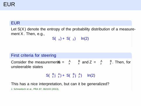
Let S(X ) denote the entropy of the probability distribution of a measure-ment X . Then, e.g.,

S(σx) + S(σz) ≥ ln(2)

First criteria for steering

Consider the measurements X = σAx ⊗ σB

x and Z = σAz ⊗ σB

z . Then, forunsteerable states

S(σBx |σA

x ) + S(σBz |σA

z ) ≥ ln(2)

This has a nice interpretation, but can it be generalized?J. Schneeloch et al., PRA 87, 062103 (2013).

EUR

EUR

Let S(X ) denote the entropy of the probability distribution of a measure-ment X . Then, e.g.,

S(σx) + S(σz) ≥ ln(2)

First criteria for steering

Consider the measurements X = σAx ⊗ σB

x and Z = σAz ⊗ σB

z . Then, forunsteerable states

S(σBx |σA

x ) + S(σBz |σA

z ) ≥ ln(2)

This has a nice interpretation, but can it be generalized?J. Schneeloch et al., PRA 87, 062103 (2013).

General criteria

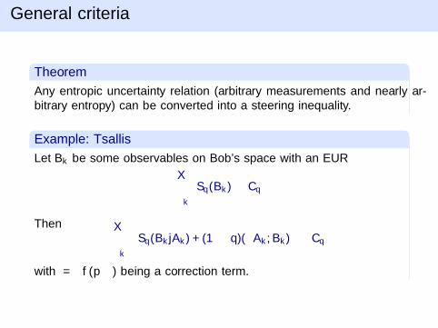
Theorem

Any entropic uncertainty relation (arbitrary measurements and nearly ar-bitrary entropy) can be converted into a steering inequality.

Example: Tsallis

Let Bk be some observables on Bob’s space with an EUR∑k

Sq(Bk) ≥ Cq

Then ∑k

[Sq(Bk |Ak) + (1− q)Γ(Ak ,Bk)

]≥ Cq

with Γ = f (pαβ) being a correction term.

General criteria

Theorem

Any entropic uncertainty relation (arbitrary measurements and nearly ar-bitrary entropy) can be converted into a steering inequality.

Example: Tsallis

Let Bk be some observables on Bob’s space with an EUR∑k

Sq(Bk) ≥ Cq

Then ∑k

[Sq(Bk |Ak) + (1− q)Γ(Ak ,Bk)

]≥ Cq

with Γ = f (pαβ) being a correction term.

Application

Isotropic states and q = 2

●

●

●

●

●●

●

■

■

■

■

■

■■

◆

◆

◆

◆

▲

▲

▲

▲

▲

▲▲

▲

● q = 2

■ Skrzypczyk and Cavalcanti

◆ Bavaresco et al.

▲ Wiseman et al.

2 4 6 80.2

0.3

0.4

0.5

0.6

d

αcrit

% = α|Φ+〉〈Φ+|+ (1− α)1

d2

Other examples: One-way steerable states

Steering: Geometric approach

The map Λ

Reminder: the task

Consider the the conditional states %a|x . Can they be written as

%a|x?=∑

λpλp(a|λ, x)σB

λ

The map

Define for a state %AB the map:

Λ(XA) = TrA(%ABXA ⊗ 1B)

For a measurement effect Ea|x one has:

%a|x = TrA(%ABEa|x ⊗ 1B) = Λ(Ea|x)

so Λ describes the steering outcomes.

The map Λ

Reminder: the task

Consider the the conditional states %a|x . Can they be written as

%a|x?=∑

λpλp(a|λ, x)σB

λ

The map

Define for a state %AB the map:

Λ(XA) = TrA(%ABXA ⊗ 1B)

For a measurement effect Ea|x one has:

%a|x = TrA(%ABEa|x ⊗ 1B) = Λ(Ea|x)

so Λ describes the steering outcomes.

Geometry of the map Λ

The effects 0 ≤ Ea|x ≤ 1 form a 4D double cone.

Λ maps it to another double cone:

Wlog: Λ is invertible.

The capacity K

For projective measurements with E+|x + E−|x = 1A on a qubit wehave to solve:

%±|x = Λ(E±|x)?=

∫dµ(σ)G±|s(σ)σ,

with G+|x + G−|x = 1 and %B = Λ(1A) =∫dµ(σ)σ.

The set of all reachable %±|x is the capacity of µ

K(µ) ={K =

∫dµ(σ)g(σ)σ : 0 ≤ g(σ) ≤ 1

}.

For a given µ the set K(µ) is convex and contains 0B and %B .

The capacity K

For projective measurements with E+|x + E−|x = 1A on a qubit wehave to solve:

%±|x = Λ(E±|x)?=

∫dµ(σ)G±|s(σ)σ,

with G+|x + G−|x = 1 and %B = Λ(1A) =∫dµ(σ)σ.

The set of all reachable %±|x is the capacity of µ

K(µ) ={K =

∫dµ(σ)g(σ)σ : 0 ≤ g(σ) ≤ 1

}.

For a given µ the set K(µ) is convex and contains 0B and %B .

Geometry

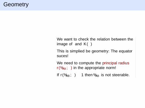
We want to check the relation between theimage of Λ and K(µ)

This is simplified be geometry: The equatorsuffices!

We need to compute the principal radiusr(%AB , µ) in the appropriate norm!

If r(%AB , µ) ≥ 1 then %AB is not steerable.

Geometry





Geometry





Geometry

For qubits, this boils down to a simple optimization problem:

r(%AB , µ) = minC

1√2‖TrB [%(1A ⊗ C )]‖

∫dµ(σ)|TrB(Cσ)|,

where % = %AB − (1A ⊗ %B)/2, ‖X‖ =√Tr(X †X ), and C denotes

an observable on Bob’s space.

Proof idea: Characterize K(µ) by linear inequalities, apply Λ−1, andproject onto equator.

Geometry

For qubits, this boils down to a simple optimization problem:

r(%AB , µ) = minC

1√2‖TrB [%(1A ⊗ C )]‖

∫dµ(σ)|TrB(Cσ)|,

where % = %AB − (1A ⊗ %B)/2, ‖X‖ =√Tr(X †X ), and C denotes

an observable on Bob’s space.

Proof idea: Characterize K(µ) by linear inequalities, apply Λ−1, andproject onto equator.

Criterion

The critical radius

The critical radius is obtained via optimization over all µ:

R(%AB) = maxµ

r(%AB , µ).

Subtle points under the carpet: R(%AB)?=∞, R(%AB) not

continuous, µ∗ exists, ...

Main result for two qubits & projective measurements

%AB is steerable ⇔ R(%AB) < 1

Remaining task: Compute the critical radius ...

Criterion

The critical radius

The critical radius is obtained via optimization over all µ:

R(%AB) = maxµ

r(%AB , µ).

Subtle points under the carpet: R(%AB)?=∞, R(%AB) not

continuous, µ∗ exists, ...

Main result for two qubits & projective measurements

%AB is steerable ⇔ R(%AB) < 1

Remaining task: Compute the critical radius ...

Scaling property of the critical radius

States mixed with separable noise %nα = α%AB + (1− α)1A ⊗ %B/2obey:

R(%nα) =1

αR(%AB).

Consequently, the border of unsteerable states can be computed:

Scaling property of the critical radius

States mixed with separable noise %nα = α%AB + (1− α)1A ⊗ %B/2obey:

R(%nα) =1

αR(%AB).

Consequently, the border of unsteerable states can be computed:

Symmetry of the critical radius

Given a state %AB , consider the family of states

% =1

N(UA ⊗ VB)%AB(U†A ⊗ V †B),

Then, the critical radius stays the same

R(%AB) = R(%)

For steerability, this was known.R. Gallego et al., PRX 2015, M. Tulio Quintino et al., PRA 2015, R. Uola et al., PRL 2014.

Under these transformations, any state can be brought into acanonical form.

Calculation of the critical radius


Idea: Approximate probability distributions on the sphere bydistributions on the vertices of an inner and outer polytope. Thisgives upper and lower bounds.

Even better: For an inner polytope with inscribed radius rin:

Rin ≤ R(%AB) ≤ Rin/rin

For a polytope with N vertices, K(µ) has O(N3) facets.

For the principal radius, there are only O(N3) possible C to check.













Steering for Babies

For a truncated icosahedron with N = 60:

rin =

√3

109(17 + 6

√5) ≈ 0.915

⇒ 60× 59× 58/6 = 34.220 linear programs with 60 variables each deter-mine the critical radius with 9% error for any state.

Result I: Random cross-sections

252 vertices, 40 min

Result I: Random cross-sections

252 vertices, 40 min

Result II: One-way steerable states

%AB = α|θ〉〈θ|+ (1− α)%A ⊗1

2with |θ〉 = cos(θ/2)|00〉+ sin(θ/2)|11〉

J. Bowles et al., PRA 2016, M. Fillettaz et al., arXiv:1804.07576.

Conclusion

Steering is an interesting problem.

Entropic uncertainty relations offer a systematic way to derivesteering criteria.

For two-qubits and projective measurements the problem can besolved with a geometric approach.

Many open problems remain: higher dimensions, POVMs, ....

Other applications: Simulatability of measurements, jointmeasureability, entropic uncertainty relations, ...

Literature

A. C.S. Costa, R. Uola, and O. Guhne, arXiv:1710.04541

H.C. Nguyen, H.-V. Nguyen, and O. Guhne, arXiv:1808.09349

Acknowledgements

Further properties

For pures states:

R(|ψ〉) =

{1/2 for entangled |ψ〉,1 for product |ψ〉.

The critical radius is neither concave or convex. The level setsQt = {%AB : R(%AB) ≥ t} are convex.

Sometimes one can calculate the gradient for R.⇒ Optimal steering inequalities

The critical radius can be defined for any operator. It is invariantunder partial transposition.⇒ Steering 6= Entanglement

Further properties

For pures states:

R(|ψ〉) =





Further properties

For pures states:

R(|ψ〉) =






For a given polytope

For any µ, the capacity K(µ) is a polytope.

For a polytope with N vertices, K has O(N3)facets.

This implies that for the pricipal radius, thereare only O(N3) possible C to check.

These C are independent of µ

All in all:O(N3) linear programs with O(N) variables.















PVMs vs POVMS

The critical radius can also be defined for higher-dimensionalsystems and POVMs.

Scaling properties still hold, but no simple evaluation.

Numerical evidence for qubits: Already the principal radius forPVMs and POVMs is the same for any µ.

0.0 0.5 1.0 1.5 2.0r2[ρ, µ]

0.0

0.5

1.0

1.5

2.0

r 4[ρ,µ

]

Documents

The geometry of EPR correlations