The Geometry of Interest Rate ModelsLecture Notes from the

Dimitsana Summer School 2005

Damir Filipovic

Department of Mathematics

University of Munich

80333 Munich, Germany

Damir.Filipovic@math.lmu.de

19 June 2006

Abstract

1 Introduction

These lecture notes give a brief overview of the geometric properties of interestrate models and their finite dimensional realizations. We consider interest ratemodels of the Heath–Jarrow–Morton (HJM) type, where the forward rates aredriven by a finite dimensional Wiener process. We will see that such models canbe realized as stochastic equations in an infinite dimensional Hilbert space H offorward curves. Within this framework it is possible to find necessary and suf-ficient conditions for the existence of finite dimensional realizations. With thiswe mean models which produce forward curves that lie in a given parametrizedcurve family with finite dimensional parameter. Such curve families arise inconnection with the estimation of the forward curve and are thus an importantobject in practice.

From a geometric point of view, these parametrized curve families can beconsidered as finite dimensional submanifolds in the Hilbert space H. Thus weare led to the problem of characterization and existence of finite dimensionalinvariant submanifolds for stochastic equations in infinite dimension.

These notes are structured as follows: Section 2 gives a brief introductionto the main terminology of interest rate models. This part is by no meansself-comprehensive. Readers without prior knowledge of the mathematics offinancial markets are advised to consult a textbook such as [1] or [12].

In Section 3 we sketch the stochastic forward rate modelling methodologyintroduced by Heath, Jarrow and Morton [14]. The main result here is theparticular form of the drift of the forward rate dynamics. We then discuss howforward curves are estimated in the market and how this requires a certain

1

consistency with the stochastic HJM model. We give an interpretation of theHJM forward rate dynamics as a curve-valued process.

This requires some theory of stochastc integrals and equations in a Hilbertspace, which is briefly reviewed in Section 4. Here we follow the lines of [6],where all proofs can be found in detail. Due to the infinite dimensionality ofH, there are several concepts of a solution to a stochastic equation: mild, weakand strong. We review them and sketch an existence and uniqueness result forweak solutions.

In Section 5 we apply these results and see how the HJM equation can beinterpreted in the context of stochastic equations in Hilbert spaces in a mildsense. As a consequence, we can restate the consistency problem for HJMmodels as a stochastic invariance problem.

In Section 6 we recall the definition and basic properties of submanifolds ina Banach space.

In Section 7 we provide the main characterization of invariant manifolds inour context.

In Section 8 we apply the general stochastic invariance results and solvethe consistency problem for HJM models stated in Section 5. The obtainedconsistency conditions are explicitely checked for the Nelson–Siegel, Svenssonand affine families.

In Section 9 we outline the theory that is used to prove existence of finitedimensional invariant manifolds. This part uses techniques involving differentialcalculus and the Frobenius theorem on Frecht spaces, which is beyond the scopeof these notes. We sketch the main ideas and results.

2 Bond Markets

In this section, we find a brief introduction to the financial terminology forinterest rate models.

One euro today is worth more than one euro tomorrow. The time t value of1 euro at time T ≥ t is expressed by the zero-coupon bond with maturityT , P (t, T ), for briefty also T -bond. This is a contract which guarantees theholder 1 euro to be paid at the maturity date T , see Figure 1.

1P(t,T)

t| |

T

Figure 1: Cashflow of a T -bond

As a consequence, future cashflows can be discounted, such as coupon-bearing bonds

C1P (t, t1) + · · · + Cn−1P (t, tn−1) + (1 + Cn)P (t, T ). (1)

2

In theory we will assume that

• there exists a frictionless market for T -bonds for every T > 0.

• P (T, T ) = 1 for all T .

• P (t, T ) is continuously differentiable in T .

In reality these assumptions are not always satisfied: zero-coupon bondsare not traded for all maturities, and P (T, T ) might be less than one if theissuer of the T -bond defaults. Yet, this is a good starting point for doing themathematics.

The third condition is purely technical and implies that the term structureof zero-coupon bond prices T 7→ P (t, T ) is a smooth curve, see Figure 2 for anexample.

1 2 3 4 5 6 7 8 9 10Years

0.2

0.4

0.6

0.8

1US Treasury Bonds, March 2002

Figure 2: Term Structure T 7→ P (t, T )

Note that t 7→ P (t, T ) is a stochastic process since bond prices P (t, T ) arenot known with certainty before t, see Figure 3.

A reasonable assumption would also be that T 7→ P (t, T ) ≤ 1 is a decreasingcurve (which is equivalent to positivity of interest rates). However, alreadyclassical interest rate models imply zero-coupon bond prices greater than 1.Therefore we leave away this requirement.

2.1 Interest Rates

A prototypical so-called forward rate agreement for t < T < S is given by thefollowing contractual terms:

• At t: sell one T -bond and buy P (t,T )P (t,S) S-bonds = zero net investment.

• At T : pay 1 euro.

• At S: obtain P (t,T )P (t,S) euros.

3

1 2 3 4 5 6 7 8 9 10t

0.2

0.4

0.6

0.8

1

PHt,10L

Figure 3: T -bond price process t 7→ P (t, T )

The net effect is a forward investment of 1 euro at time T yielding P (t,T )P (t,S) euros

at S. The corresponding continuously compounded forward rate for [T, S]prevailing at t is defined as

eR(t;T,S)(S−T ) :=P (t, T )

P (t, S)⇔ R(t;T, S) = − log P (t, S) − log P (t, T )

S − T.

As we let S tend to T , we arrive at the (instantaneous) forward rate withmaturity T prevailing at time t, which is defined as

f(t, T ) := limS↓T

R(t;T, S) = −∂ log P (t, T )

∂T⇔ P (t, T ) = exp

(−

∫ T

t

f(t, u) du

).

The function x 7→ f(t, t + x) is called the forward curve at time t. We callf(t, t) the (instantaneous) short rate at time t.

The bank account B(t) is the asset which grows at time t instantaneouslyat short rate f(t, t). That is,

dB(t) = f(t, t)B(t)dt.

With B(0) = 1 we obtain

B(t) = exp

(∫ t

0

f(s, s) ds

).

B is important for relating amounts of currencies available at different times:in order to have 1 euro in the bank account at time T we need to have

B(t)

B(T )= exp

(−

∫ T

t

f(s, s) ds

)

euros in the bank account at time t ≤ T . Note that this discount factor isstochastic.

4

3 HJM Methodology

In this section, we sketch the stochastic forward rate modelling methodologyprovided by Heath–Jarrow–Morton (HJM) in [14].

Throughout these notes, we fix a stochastic basis (Ω,F , (Ft), P), satisfyingthe usual conditions, carrying a d-dimensional Brownian motion W .

For every T > 0, we let the forward rate

f(t, T ) = f(0, T ) +

∫ t

0

αf (s, T ) ds +

∫ t

0

σf (s, T ) dW (s), t ∈ [0, T ] (2)

follow an Ito process.Heath, Jarrow and Morton [14] respond to the following question: what are

sufficient conditions on the dynamics (2) such that the implied bond market

P (t, T ) = exp

(−

∫ T

t

f(t, s) ds

)

is arbitrage-free? With arbitrage we mean any self-financing strategy, that is,a predictable process

(φ1, . . . , φn),

yielding a profit without risk, that is,

V (T ) := B(T )∑

i

∫ Ti

0

φi(t) d

(P (t, Ti)

B(t)

)≥ 0 and P[V (T ) > 0] > 0,

for some n ∈ N and 0 < T1 < · · · < Tn ≤ T . For more background on thestochastics of arbitrage-free financial markets, we refer to [1].

For illustration of what arbitrage and its absence means, we consider a de-terministic world. That is, all bond prices P (t, T ) are known (deterministic).In this case, absence of arbitrage holds if and only if

P (t, S) = P (t, T )P (T, S), ∀t ≤ T ≤ S. (3)

This is equivalent to

f(t, T ) = f(0, T ), ∀t ∈ [0, T ]. (4)

Indeed, suppose that P (t, S) > P (t, T )P (T, S). Then selling 1 S-bond andbuying P (T, S) T -bonds at t results in a strict positive net gain by time Swithout any risk of loss. This is an arbitrage strategy, which is exluded byassumption. By changing signs, one shows that also P (t, S) < P (t, T )P (T, S)is impossible, whence (3).

The Fundamental Theorem of Asset Pricing (proved in full generalityin [7], see e.g. [1, 12]) states that there is no arbitrage if and only if there existsan equivalent probability measure Q ∼ P such that

(P (t, T )

B(t)

)

t∈[0,T ]

is a Q-local martingale, for all T > 0. (5)

5

As a consequence, under some additional technical conditions

P (t, T ) = EQ

[1

B(T )| Ft

]

is the fair price of 1 euro at T .Heath, Jarrow and Morton show in [14] that – under some technical condi-

tions – (5) is equivalent to the HJM Drift Condition

αf (t, T ) = σf (t, T ) ·∫ T

t

σf (t, u) du, ∀t ≤ T, (6)

under Q and for the respective Girsanov transform of W in (2). For pricingpurposes, one therefore usually assumes that Q = P already satsifes (5).

3.1 From HJM to Stochastic Equations

The forward curve x 7→ f(t, t + x) cannot be directly observed on the market.The forward curve has to be estimated, on a day-by-day basis, from coupon-bearing bond prices (1) and other related data. Formally, the forward curveis estimated by a parametrized family of curves x 7→ G(x; z), for some deter-ministic smooth function G : R+ ×Z → R and a finite-dimensional state spaceZ ⊂ Rm. Most prominent examples are the Nelson–Siegel family ([17])

GNS(x; z) = z1 + z2e−z4x + z3xe−z4x

and Svensson family ([18])

GS(x; z) = z1 + (z2 + z3x) e−z5x + z4xe−z6x.

That way, a time series for z ∈ Z is observed which can be used to calibratea stochastic model Z(t). This in turn implies an accurate factor model for theforward curve, f(t, t + x) = G(x;Z(t)). An important question arises: canthis factor modelling be made consistent with the HJM methodology outlinedabove? In other words, what are the conditions on G(x; z) and the dynamics ofZ(t) such that the resulting forward curve model f(t, T ) is arbitrage-free, i.e.satisfies the HJM drift condition (6)?

As a first step, we have to understand the HJM dynamics of t 7→ f(t, t + ·)as a curve-valued process. We therefore let S(t) | t ≥ 0 denote the semigroupof right shifts, S(t)g(x) := g(x + t), and rewrite (2)

f(t, x+t) = S(t)f(0, x)+

∫ t

0

S(t−s)αf (s, x+s) ds+

∫ t

0

S(t−s)σf (s, x+s) dW (s).

Hence the function valued process r(t) = r(t, ·) : R+ → R defined by

r(t, x) := f(t, t + x) (7)

6

satisfies

r(t) = S(t)r(0) +

∫ t

0

S(t − s)α(s) ds +

∫ t

0

S(t − s)σ(s) dW (s)

whereα(s, x) := αf (s, s + x), σ(s, x) := σf (s, s + x). (8)

As we will see in Section 4 below, it follows that r(t) can be interpreted as mildsolution of the stochastic equation

dr(t) =

(d

dxr(t) + α(t)

)dt + σ(t) dW (t).

The parametrization (7) and the interpretation of r as solution of a stochasticPDE was first suggested by Musiela [16]. An infinite dimensional stochasticanalysis perspective on HJM models is also given in the recent book by Carmonaand Tehranchi [4].

4 Stochastic Equations in Infinite Dimensions

In this intermediary section, we provide a short introduction to stochastic equa-tions in infinite dimensions. A thorough treatment can be found in [6]. Through-out, we let H be a separable Hilbert space, and S(t) | t ≥ 0 denotes a stronglycontinuous semigroup on H, that is,

S(t) : H → H bounded linear, S(t + s) = S(t)S(s), S(0) = Id,

t 7→ S(t)h continuous for all h ∈ H,

with infinitesimal generator A : D(A) → H, defined as

Ah = limt→0+

S(t)h − h

t, D(A) := h ∈ H | Ah exists in H .

It is well known that D(A) is dense in H. In fact, for any h ∈ H we have∫ t

0S(u)h du ∈ D(A) with limt→0+

1t

∫ t

0S(u)h du = h. We denote by A∗ :

D(A∗) → H the adjoint of A, defined as follows:

D(A∗) := h ∈ H | g 7→ 〈Ag, h〉 is continuous on D(A).

By the Hahn–Banach theorem, for every h ∈ D(A∗), there exists then a uniqueelement A∗h ∈ H with 〈g,A∗h〉 = 〈Ag, h〉 for all g ∈ D(A). By reflexivity of H,we have A∗∗ = A and D(A∗) is dense in H.

We let F : H → H and B : H → Hd be continuous mappings. A stochasticequation in H is

dX(t) = (AX(t) + F (X(t))) dt + B(X(t)) dW (t)

X(0) = h0.(9)

7

The stochastic integral in H can be defined for all Y ∈ L where

L :=

Y Hd-valued predictable |

∫ T

0

‖Y (t)‖2Hddt < ∞ a.s. for all T < ∞

.

Indeed, the construction is just as in Rd. We remark that it is also possible todefine an infinite dimensional Brownian motion and its stochastic integrals, see[6]. This, however, requires additional effort and is beyond the scope of thesenotes.

Write

L2T :=

Y ∈ L | E

[∫ T

0

‖Y (t)‖2Hd dt

]< ∞

.

We now quote four technical lemmas. For a proof see [6].

Lemma 4.1. For Y ∈ L2T we have

E

∥∥∥∥∥

∫ T

0

Y (t) dW (t)

∥∥∥∥∥

2

H

= E

[∫ T

0

‖Y (t)‖2Hd dt

].

Lemma 4.2 (Stochastic Fubini Theorem). Let (E, E , µ) be a probabilityspace and let

Y : ([0, T ] × Ω × E,P ⊗ E) → (Hd,B(Hd)), (t, ω, x) 7→ Y (t, ω, x)

be a measurable mapping with

∫ T

0

∫

E

‖Y (t, ω, x)‖2Hd µ(dx) dt < ∞ a.s.

Then there exists an FT⊗E-measurable version of the stochastic integral∫ T

0Y (t, x) dW (t)

which is µ-integrable a.s. and

∫

E

∫ T

0

Y (t, x) dW (t)µ(dx) =

∫ T

0

∫

E

Y (t, x)µ(dx) dW (t) a.s.

Lemma 4.3. Let Y ∈ L, then

Z(t) =

∫ t

0

S(t − s)Y (s) dW (s)

has a predictable version.

Lemma 4.4. Let Y be an H-valued predictable process. Then the random setY ∈ D(A) and

Z(t, ω) :=

AY (t, ω), if Y (t, ω) ∈ D(A)

0, else

are predictable.

8

4.1 Solution Concepts

Due to the infinite dimensionality of H and the unboundedness of A, there areseveral concepts of a solution to (9). Indeed, let X be an H-valued predictableprocess and τ > 0 a stopping time with

∫ t∧τ

0

(‖X(s)‖H + ‖F (X(s))‖H + ‖B(X(s))‖2

Hd

)< ∞ a.s. ∀t < ∞.

We call X a

(i) local mild solution of (9) if

X(t) = S(t)h0+

∫ t

0

S(t−s)F (X(s)) ds+

∫ t

0

S(t−s)B(X(s)) dW (s) ∀t ≤ τ

(ii) local weak solution of (9) if, for all ζ ∈ D(A∗),

〈ζ,X(t)〉 = 〈ζ, h0〉 +

∫ t

0

(〈A∗ζ,X(s)〉 + 〈ζ, F (X(s))〉) ds

+

∫ t

0

〈ζ,B(X(s))〉dW (s) ∀t ≤ τ

(iii) local strong solution of (9) if X ∈ D(A) dt⊗dP-a.s.,∫ t∧τ

0‖AX(s)‖ ds <

∞ a.s. and

X(t) = h0 +

∫ t

0

(AX(s) + F (X(s))) ds +

∫ t

0

B(X(s)) dW (s) ∀t ≤ τ.

The stopping time τ is called the life time of X. If τ = ∞ then we skip theword “local” in the above definitions.

Remark 4.5. In view of Lemma 4.3 we understand that the implicitly t-dependentstochastic integral in (i) is predictable. Moreover, the integrand AX in (iii) isto be interpreted in the sense of Lemma 4.4.

The next lemmas state how these concepts of a solution are related.

Lemma 4.6. strong ⇒ weak.

Proof. Follows from U∫

Y dW =∫

UY dW if U ∈ L(H;E), Y ∈ L.

Lemma 4.7. weak ⇒ mild.

Proof. Let ζ ∈ D(A∗), φ ∈ C1([0, T ]; R). Then

d〈ζφ(t),X(t)〉 = d (〈ζ,X(t)〉φ(t))

= (〈ζφ′(t) + A∗ζφ(t),X(t)〉 + 〈ζφ(t), F (X(t))〉) dt + 〈ζφ(t), B(X(t))〉dW (t)

9

Since the elements ζ(t) = ζφ(t) lie dense in C1([0, T ];D(A∗)) we have

〈ζ(t),X(t)〉 =

∫ t

0

(〈ζ ′(s) + A∗ζ(s),X(s)〉 + 〈ζ(s), F (X(s))〉) ds

+

∫ t

0

〈ζ(s), B(X(s))〉dW (s)

for all ζ ∈ C1([0, T ];D(A∗)). In particular, for ζ(s) := S∗(t − s)ζ with ζ ∈D(A∗), we have

ζ ′(s) = −A∗ζ(s)

and hence

〈ζ,X(t)〉 =

∫ t

0

〈ζ, S(t − s)F (X(s))〉ds +

∫ t

0

〈ζ, S(t − s)B(X(s))〉dW (s).

Since D(A∗) is dense in H, the claim follows.

Lemma 4.8. If B(X) ∈ L2T , then mild ⇒ weak.

Proof. For simplicity we assume F = 0. Write

Y (t) :=

∫ t

0

S(t − s)B(X(s)) dW (s).

By assumption the stochastic Fubini theorem 4.2 applies:

∫ t

0

〈A∗ζ, Y (s)〉 ds =

∫ t

0

∫ s

0

〈A∗ζ, S(s − u)B(X(u))〉 dW (u)ds

=

∫ t

0

⟨A∗ζ,

∫ t

u

S(s − u)B(X(u)) ds

⟩dW (u)

=

∫ t

0

⟨ζ,A

∫ t−u

0

S(s)B(X(u)) ds

⟩dW (u)

=

∫ t

0

〈ζ, S(t − u)B(X(u)) − B(X(u))〉 dW (u)

= 〈ζ, Y (t)〉 −∫ t

0

〈ζ,B(X(u))〉 dW (u),

for all ζ ∈ D(A∗).

In view of Lemmas 4.6–4.8 it is obvious that the above solution conceptscoincide if A is bounded, which is in particular the case if H is finite-dimensional.

10

4.2 Existence and Uniqueness

For proving existence of a solution to (9) we will use a fix point argument.

Definition 4.9. G : H → E is (locally) Lipschitz continuous if (for alln ∈ N)

‖G(x) − G(y)‖E ≤ C‖x − y‖H

for all x, y ∈ H (with ‖x‖ ≤ n, ‖y‖ ≤ n) and a constant C (C = C(n)).

The following result is from Theorem 7.4 in [6]. We will sketch the proofbelow.

Theorem 4.10. Suppose F and B are Lipschitz continuous. Then, for all h0 ∈H, there exists a unique continuous weak solution X = Xh0 of (9). Moreover,for every p ≥ 2 and T < ∞, there exists a constant K = K(p, T ) with

E

[sup

t∈[0,T ]

‖X(t)‖pH

]≤ K (1 + ‖h0‖p

H) . (10)

This existence result can be localized.

Corollary 4.11. Suppose F and B are locally Lipschitz continuous. Then, forall h0 ∈ H, there exists a unique continuous local weak solution X = Xh0 of (9).

Proof of Corollary 4.11. Let h0 ∈ H. Set R := 2‖h0‖H and define

F (h) := F ((R/‖h‖H ∧ 1)h), B(h) := B((R/‖h‖H ∧ 1)h).

Then F and B are Lipschitz continuous. Hence there exists a unique continuousweak solution X of

dX =(AX + F (X)

)dt + B(X) dW, X(0) = h0.

Define the stopping time τ := inft ≥ 0 | ‖X(t)‖H ≥ R. Then τ > 0 and

X(t) := X(t ∧ τ) is a continuous local weak solution of (9) with lifetime τ .If X is a continuous local weak solution of (9) then, by the above arguments,

it is unique on [0, τn] for n ≥ 2 where τn := inft ≥ 0 | ‖X(t)‖H ≥ n‖h0‖. Nowuse that τn ↑ ∞.

Sketch of Proof of Theorem 4.10. Uniqueness: let X1, X2 be two mild solutionsof (9). Fix R > 0 and define the stopping time

τ := inf

t ≤ T |

∫ t

0

‖F (Xi(s))‖H ds ≥ R or

∫ t

0

‖B(Xi(s))‖2Hd ds ≥ R for i = 1 or i = 2

.

11

Then Xτi (t) := Xi(t ∧ τ) satisfy

Xτ1 (t) − Xτ

2 (t) =

∫ t∧τ

0

S(t ∧ τ − s) (F (Xτ1 (s)) − F (Xτ

2 (s))) ds

+

∫ t∧τ

0

S(t ∧ τ − s) (B(Xτ1 (s)) − B(Xτ

2 (s))) dW (s)

and hence

E[‖Xτ

1 (t) − Xτ2 (t)‖2

H

]≤ CE

[(∫ t∧τ

0

‖F (Xτ1 (s)) − F (Xτ

2 (s))‖H ds

)2]

+ CE

[∫ t∧τ

0

‖B(Xτ1 (s)) − B(Xτ

2 (s))‖2Hd ds

]

≤ C

∫ t

0

E[‖Xτ

1 (s) − Xτ2 (s)‖2

H

]ds.

Gronwall’s Lemma (0 ≤ f(t) ≤ ε + M∫ t

0f(s) ds ⇒ f(t) ≤ εeMt) implies

E[‖Xτ

1 (t) − Xτ2 (t)‖2

H

]= 0. This is true for all R > 0, hence X1(t) = X2(t)

a.s. for all t.Existence: Let p ≥ 2 and define the Banach space of H-valued predictable

processes Hp with norm

‖Y ‖pp := sup

t∈[0,T ]

E [‖Yt‖pH ] .

One can show that

K(Y )(t) := S(t)h0 +

∫ t

0

S(t − s)F (Y (s)) ds +

∫ t

0

S(t − s)B(Y (s)) dW (s)

maps Hp into Hp and ‖K(Y1) −K(Y2)‖p ≤ C(T )‖Y1 − Y2‖p.The constant C(T ) is independent of the initial condition h0 and can be made

< 1 for T small enough. Then K has a unique fix point X in Hp. One thenproceeds for [0, T ], [T, 2T ],. . . (with random initial condition) to derive globalexistence.

Notice that E [‖X(t)‖p] ≤ C(T, p)(‖h0‖p +

∫ t

0E [‖X(s)‖p] ds

), ∀t ≤ T .

Hence Gronwall’s Lemma implies (10). From Lemma 4.8 we deduce that Xis a weak solution.

Finally, from Lemma 4.12 below we obtain a continuous modification of X,whence the theorem is proved.

Lemma 4.12. Let Y ∈ L2T with E

[∫ T

0‖Y (t)‖p

Hd dt]

< ∞, and write

Z(t) :=

∫ t

0

S(t − s)Y (s) dW (s), Zn(t) := eAnt

∫ t

0

e−AnsY (s) dW (s)

12

where the bounded linear operators An := nA∫

e−ntS(t) dt = nA(n − A)−1 arethe Yosida approximations (limn Anx = Ax if x ∈ D(A)). Then

limn

E

[sup

t∈[0,T ]

‖Z(t) − Zn(t)‖p

]= 0.

Hence Z has a continuous modification.

Sketch of Proof of Lemma 4.12. Let α ∈ (1/p, 1/2), and write (stochastic Fu-bini)

Z(t) =sin(πα)

π

∫ t

0

∫ t

u

(t − s)α−1(s − u)−α ds

︸ ︷︷ ︸= π

sin(πα)

S(t − u)︸ ︷︷ ︸=S(t−s)S(s−u)

Y (u) dW (u)

=sin(πα)

π

∫ t

0

(t − s)α−1S(t − s)

∫ s

0

(s − u)−αS(s − u)Y (u) dW (u)

︸ ︷︷ ︸=:U(s)

ds

Using Holder’s inequality (α > 1/p ⇒ (α − 1)p/(p − 1) > −1), we deduce

supt∈[0,T ]

‖Z(t)‖p ≤ C supt∈[0,T ]

(∫ t

0

(t − s)(α−1)p

p−1 ds

)p−1 ∫ T

0

‖U(s)‖pH ds.

Moreover, from [6, Lemma 7.2] and Young’s convolution inequality,

∫ T

0

E [‖U(s)‖pH ds] ≤ CE

[∫ T

0

‖Y (u)‖p

Hd du

].

Define Un(s) for Zn as above, and decompose

Z(t) − Zn(t) =sin(πα)

π

∫ t

0

(S(t − s) − e(t−s)An

)(t − s)α−1U(s) ds

+sin(πα)

π

∫ t

0

e(t−s)An(t − s)α−1 (U(s) − Un(s)) ds =: In(t) + Jn(t).

Eventually, one can show that

E

[sup

t∈[0,T ]

‖In(t)‖pH

]→ 0 and E

[sup

t∈[0,T ]

‖Jn(t)‖pH

]→ 0.

5 Forward Curve Space

In order to carry over the HJM methodology to the above stochastic equationframework, we need to define a reasonable Hilbert space. Since in practice

13

the forward curve is obtained by smoothing data points using smooth fittingmethods it is reasonable to assume

∫

R+

| d

dxr(t, x)|2 dx < ∞.

Moreover, the curve flattens for large time to maturity x. There is no reason tobelieve that the forward rate for an instantaneous loan that begins in 10 yearsdiffers much from one which begins one day later. We take this into accountby penalizing irregularities of rt(x) for large x by some increasing weightingfunction w(x) ≥ 1, that is,

∫

R+

| d

dxr(t, x)|2 w(x)dx < ∞.

However, this does not define a norm yet since constant functions are not dis-tinguished. So we add the square of the short rate |r(t, 0)|2.

Let us recall a few facts from real analysis. Let h ∈ L1loc(R+). The weak

derivative h′ ∈ L1loc(R+) of h, if it exists, is uniquely specified by the property

∫

R+

h(x)ϕ′(x) dx = −∫

R+

h′(x)ϕ(x) dx, ∀ϕ ∈ C1c ((0,∞)).

If h has a weak derivative h′ then there exists an absolutely continuous repre-sentative of h, still denoted by h, such that

h(x) − h(y) =

∫ x

y

h′(u) du, ∀x, y ∈ R+. (11)

Accordingly, the following definition makes sense.

Definition 5.1. Let w ∈ C1(R+; [1,∞)) be increasing such that

w− 13 ∈ L1(R+). (12)

We write

‖h‖2w := |h(0)|2 +

∫

R+

|h′(x)|2 w(x)dx

and define

Hw :=h ∈ L1

loc(R+) | ∃h′ ∈ L1loc(R+) and ‖h‖w < ∞

.

The choice of Hw is established by the next theorem.

Theorem 5.2. Hw equipped with ‖ · ‖w is a separable Hilbert space satisfying

(H1) Hw ⊂ C(R+; R) and Jx(h) := h(x) is continuous

(H2) S(t)f(x) := f(x + t), t ≥ 0, is a strongly continuous semigroup withinfinitesimal generator d/dx and D(d/dx) = h ∈ Hw | h′ ∈ Hw

14

(H3) ‖Sh‖w ≤ K‖h‖2w ∀h ∈ Hw,0 for some constant K where

Hw,0 := h ∈ Hw | h(∞) = 0, Sf(x) := f(x)

∫ x

0

f(y) dy. (13)

Moreover, S : Hw,0 → Hw,0 is locally Lipschitz continuous.

Remark 5.3. The definition (13) of S becomes clear in view of the HJM driftcondition (6) and (8). Indeed, (6) simply translates to

α =

d∑

j=1

Sσj . (14)

Examples of admissible weighting functions w which satisfy condition (12):

Example 1 w(x) = eαx, for α > 0.

Example 2 w(x) = (1 + x)α, for α > 3.

5.1 HJM Revisited

Now let σ : Hw → Hdw,0 be locally Lipschitz continuous. From Theorem 5.2 we

conclude thatα :=

∑

j

Sσj : Hw → Hw

is locally Lipschitz continuous. Hence σ fully determines a HJM model.

Theorem 5.4. The continuous weak solution r (if it exists globally) of

dr(t) =

(d

dxr(t) + α(r(t))

)dt + σ(r(t)) dW (t)

r(0) = r0

(15)

induces an arbitrage-free bond market

P (t, T ) = exp

(−

∫ T−t

0

r(t, x) dx

)

with initial term structure P (0, T ) = exp(−

∫ T

0r0(x) dx

).

Idea of Proof. Show that f(t, T ) = r(t, T − t) and P (t, T ), 0 ≤ t ≤ T , are Itoprocesses, and apply the HJM drift condition (14). See [8, Section 4].

Remark 5.5. Recall the deterministic case (σ = 0) in (4): ddt

r(t, x) = ddx

r(t, x).

15

5.2 Back to the Consistency Problem

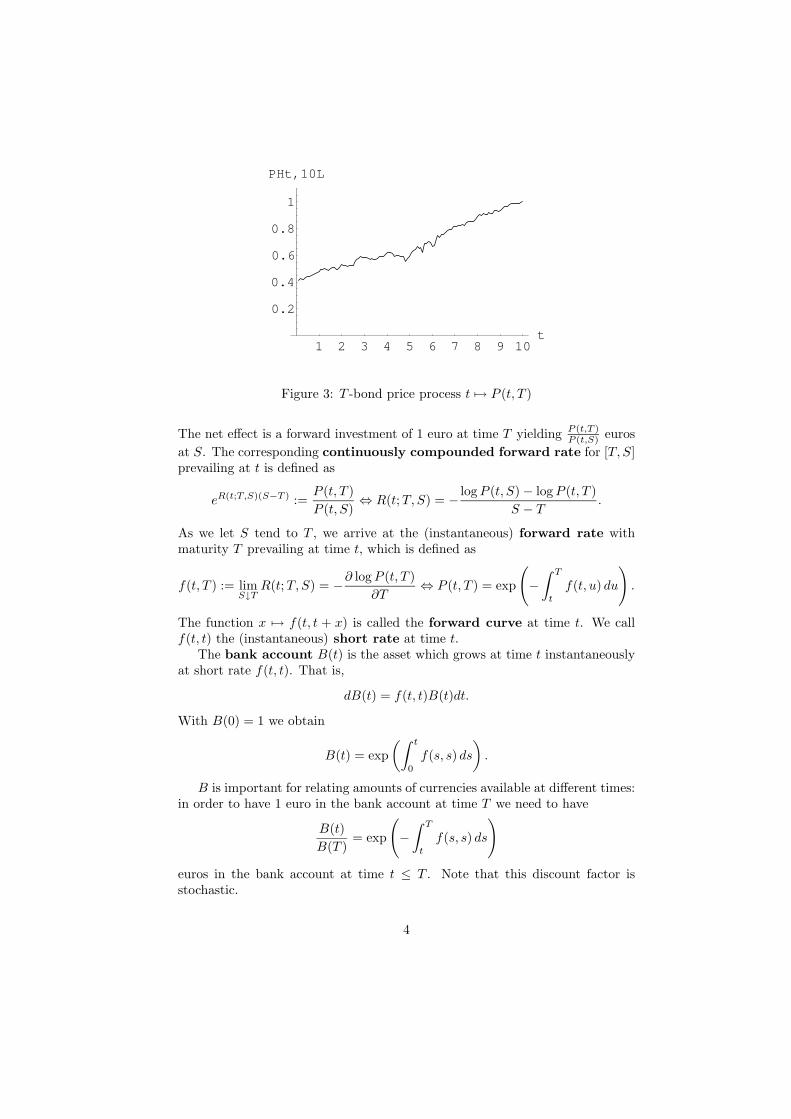
We can now restate the consistency problem of Section 3.1: is there a HJMmodel σ which is consistent with the Nelson–Siegel family G = GNS? In otherwords, can we find an R4-valued diffusion process Z and a volatility map σ suchthat

r(t, x) = G(x;Z(t))

solves the corresponding HJM equation (15)? Bjork et al. [2, 3] translate this

G

H

R^d

Z(t)

r(t)r(0)

Z(0)

G(R^d)

Figure 4: Geometric View of the Consistency Problem

in a geometric problem: consider G := G(Z) as submanifold in Hw and checkwhether G is invariant under the stochastic dynamic equation (15), see Figure 4.This is a stochastic invariance problem.

6 Submanifolds in Banach Spaces

For the convenience of the reader, we give a brief introduction to submanifolds.We follow [8, Section 6.1]. All proofs can be found there.

Let E denote a reflexive Banach space, E′ its dual space, 〈e′, e〉 the dualitypairing. For a direct sum decomposition E = E1 ⊕ E2 we denote by Π(E2,E1)

the induced projection onto E1.

Definition 6.1. A subset M ⊂ E is an m-dimensional (regular) Ck sub-manifold with boundary of E, if for all h ∈ M there is a neighborhood U inE, an open set V ⊂ Rm

≥0 := ym ≥ 0 and a Ck map φ : V → E such that

(i) φ : V → U ∩M is a homeomorphism, and φ(V ∩ ym = 0) = U ∩ ∂M(hence ∂M is a submanifold)

16

(ii) Dφ(y) is one to one for all y ∈ V .

The map φ is called a parametrization in h.M is a linear submanifold if for all h ∈ M there exists a linear parametriza-

tion of the form φ(y) = h +∑m

i=1 yiei in h.

In what follows, M denotes an m-dimensional Ck submanifold with bound-ary of E (k ≥ 2). Using the inverse mapping theorem, one can show that Mshares the characterizing property of a Ck manifold:

Lemma 6.2. Let φi : Vi → Ui ∩M, i = 1, 2, be two parametrizations such thatW := U1 ∩ U2 ∩M 6= ∅. Then the change of parameters

φ−11 φ2 : φ−1

2 (W ) → φ−11 (W )

is a Ck diffeomorphism.

Definition 6.3. For h ∈ M the tangent space to M at h is the subspace

ThM := Dφ(y)Rm, y = φ−1(h),

where φ : V ⊂ Rm → M is a parametrization in h. Moreover,

Th∂M = Dφ(y)zm = 0, ThM≥0 := Dφ(y)Rm≥0, h ∈ ∂M.

By Lemma 6.2, the definition of ThM is independent of the choice of theparametrization.

A vector field X : M 3 h 7→ X(h) ∈ ThM can be represented locally as

X(h) = Dφ(y)α(y), y = φ−1(h), ∀h ∈ U ∩M, (16)

where φ : V → U ∩M is a parametrization and α is an Rm-valued vector fieldon V (uniquely determined by φ).

Definition 6.4. The vector field X is of class Cr, 0 ≤ r < k, if for anyparametrization φ the corresponding Rm-valued vector field α in (16) is of classCr.

Again by Lemma 6.2 this is a well defined concept.

Remark 6.5. The above definitions and properties of submanifolds carry over toFrechet spaces E, which we will consider in Section 9 below. We note, however,that differential calclulus is more difficult on such general spaces.

For further use, we may and will assume that any parametrization φ : V →U ∩M extends to φ ∈ Ck

b (Rm;E): let h ∈ U ∩M and y = φ−1(h). There existsε > 0 such that the open ball B2ε(y) = v ∈ Rm | |y − v| < 2ε is containedin V . On B2ε(y) one can define a function ψ ∈ C∞(Rm; [0, 1]) satisfying ψ ≡ 1on Bε(y) and supp(ψ) ⊂ B2ε(y). Since φ is a homeomorphism there exists anopen neighborhood U ′ of h in E with φ(Bε(y)) = U ′ ∩M. Set φ := ψφ. Thenφ ∈ Ck

b (Rm;E) and φ|Bε(y) = φ|Bε(y) : Bε(y) → U ′ ∩M is a parametrization inh.

The following result is crucial for our discussion of weak solutions to stochas-tic equations viable in M.

17

Proposition 6.6. Let D ⊂ E′ be a dense subset. Then for any h ∈ M thereexist linearly independent elements e′1, . . . , e

′m in D and a parametrization φ :

V → U ∩M in h such that

φ(〈e′1, z〉, . . . , 〈e′m, z〉) = z, ∀z ∈ U ∩M.

Moreover,E = ThM⊕ E2, ∀h ∈ U ∩M,

where E2 :=⋂m

i=1 ker(e′i), and the induced projections are given by

Π(E2,ThM) = Dφ(y)(〈e′1, ·〉, . . . , 〈e′m, ·〉), y = φ−1(h), ∀h ∈ U ∩M. (17)

Idea of Proof. The idea is to find a decomposition E = E1 ⊕ E2, dim E1 = m,such that E1 is “not too far” from ThM and such that

Π(E2,E1) = 〈e′1, ·〉e1 + · · · + 〈e′m, ·〉em

with e′1 . . . , e′m ∈ D. Thereby the expression “not too far” means that Π(E2,E1)|ThM :ThM → E1 is an isomorphism.

Let B ∈ C1(E;E) be such that B(h) ∈ ThM; that is, B|M is a C1 vectorfield on M. Let h ∈ M and y = φ−1(h). Then

c(t) := φ(y + tDφ(y)−1B(h))

satisfiesd

dtB(c(t))|t=0 = DB(h)B(h). (18)

On the other hand, in view of (17) we have

d

dtB(c(t))|t=0 =

d

dtDφ(〈e′, c(t)〉)〈e′, B(c(t))〉|t=0

= D2φ(y)(〈e′, B(h)〉, 〈e′, B(h)〉) + Dφ(y)〈e′,DB(h)B(h)〉. (19)

We have thus proved:

Lemma 6.7.

DB(h)B(h) = Dφ(y)〈e′,DB(h)B(h)〉 + D2φ(y)(〈e′, B(h)〉, 〈e′, B(h)〉)

is the decomposition according to E = ThM⊕ E2, for all h ∈ U ∩M.

7 Invariant Manifolds

In this section we provide the main characterization of invariant manifolds in ourcontext. In what follows, we let M denote an m-dimensional C2 submanifoldof H. We follow [8, Section 6.2]. All proofs can be found there.

18

Since H is separable, there exists a countable open covering (Uk)k∈N of Mand for each k a parametrization φk : Vk ⊂ Rm → Uk ∩ M, where φk ∈C2

b (Rm;H).Moreover, since D(A∗) is dense in H, by Proposition 6.6 we can assume that

for each k there exists a linearly independent set ζk,1, . . . , ζk,m in D(A∗) suchthat

φk(〈ζk,1, h〉, . . . , 〈ζk,m, h〉) = h, ∀h ∈ Uk ∩M. (20)

Notation: we write 〈ζk, h〉 instead of (〈ζk,1, h〉, . . . , 〈ζk,m, h〉).Now consider the stochastic equation in H

dX(t) = (AX(t) + F (X(t))) dt + B(X(t)) dW (t)

X(0) = h0.(21)

Assumption: B ∈ C1(H;Hd) and F locally Lipschitz continuous.In view of Corollary 4.11 there exists a unique continuous local weak solution

X of (21) with life time τ > 0.We know that in finite-dimensional spaces, weak solutions are strong so-

lutions. This fact carries over to the non-linear case of a finite-dimensionalmanifold.

Theorem 7.1 (Regularity). Suppose

X(t) ∈ M ∀t ≤ τ.

Then X is a local strong solution of (21).

Conversely, it turns out that an invariant manifold has to lie in D(A). Wefirst give a rigorous definition of stochastic invariance.

Definition 7.2. M is called locally invariant for (21) if, for all h0 ∈ M,there exists a stopping time τ = τ(h0) > 0 with Xh0(t) ∈ M for all t ≤ τ .

We now obtain the familiar tangent conditions for stochastic invariance asin the finite-dimensional case.

Theorem 7.3 (Main Characterization). The following are equivalent:

(i) M is locally invariant for (21)

(ii) M ⊂ D(A) and

Ah + F (h) − 1

2

∑

j

DBj(h)Bj(h) ∈ ThM (ThM≥0) (22)

Bj(h) ∈ ThM (Th∂M) (23)

for all h ∈ M (h ∈ ∂M).

If, in addition, M is closed then X(t) ∈ M for all t ≥ 0.

19

A key step in proving Theorem 7.3 is the following lemma, wich is based onLemma 6.7.

Lemma 7.4. Suppose U∩M ⊂ D(A), and let φ : V → U∩M be a parametriza-tion satisfying (20). Then (22) and (23) hold for all h ∈ U ∩ M if and onlyif

Ah + F (h) = Dφ(h) (〈A∗ζ, h〉 + 〈ζ, F (h)〉)

+1

2

∑

j

D2φ(y) (〈ζ,Bj(h)〉〈ζ,Bj(h)〉) (24)

Bj(h) = Dφ(y)〈ζ,Bj(h)〉, (25)

where y = 〈ζ, h〉, for all h ∈ U ∩M.

7.1 Consistency Conditions in Local Coordinates

For applications it is convenient to express the consistency conditions (22) and(23) in local coordinates.

Assume M is locally invariant for (21). Let φ : V → U ∩ M be anyparametrization, and define

Dφ(y)β(y) := Aφ(y) + F (φ(y)) − 1

2

∑

j

DBj(φ(y))Bj(φ(y)),

Dφ(y)ρj(y) := Bj(φ(y))

(26)

(β(y) ∈ Rm≥0 and ρj(y) ∈ zm = 0 if ym = 0). As shown above

DBj(φ(y))Bj(φ(y)) =d

dtBj (φ(y + tρj(y))) |t=0

=d

dt(Dφ(y + tρj(y))ρj(y + tρj(y))) |t=0

= D2φ(y) (ρj(y), ρj(y)) + Dφ(y) (Dρj(y)ρj(y))

Plugging this in (26), we obtain

Theorem 7.5. Consistency conditions (22)–(23) hold for all h ∈ U ∩M if andonly if

Aφ(y) + F (φ(y)) − 1

2

∑

j

D2φ(y) (ρj(y), ρj(y)) = Dφ(y)b(y) (27)

Bj(φ(y)) = Dφ(y)ρj(y) (28)

for all y ∈ V , where b(y) := β(y) + 12

∑j Dρj(y)ρj(y).

Moreover, X is a continuous local strong solution of (21) in U ∩M if andonly if X = φ(Y ) where

dY (t) = b(Y (t)) dt + ρ(y(t)) dW (t), Y (0) = φ−1(X(0)). (29)

20

8 Consistent Forward Curve Families

We now apply the above general results on stochastic invariance and solve theconsistency problem for HJM models stated in Section 5.2.

Let G ∈ C2(Rm;Hw) be a parametrized forward curve family, and supposethat G : V ⊂ Rm → G(V ) is a parametrization.

Assume σ ∈ C1(Hw;Hdw,0), and remember the HJM equation, with α =∑

j S(σj):

dr(t) =

(d

dxr(t) + α(r(t))

)dt + σ(r(t)) dW (t)

r(0) = r0.

(30)

We say that G is consistent with the HJM model σ if G(V ) is locally invariantfor (30). From Theorem 7.5 we can deduce the following explicit consistencycondition.

Theorem 8.1. G is consistent with the HJM model σ if and only if there existb : V → Rm and ρ : V → Rm×d continuous such that

∂xG(x, z) = b(z) · ∇zG(x, z)

+∑

k,l

akl(z)

(1

2∂zk

∂zlG(x, z) − ∂zk

G(x, z)

∫ x

0

∂zlG(y, z) dy

)(31)

for all (x, z) ∈ R+ × V , where a := ρT · ρ is the diffusion matrix.

The consistency condition (31) can be explicitely checked, and we will dothis below for the Nelson–Siegel, Svensson and affine families.

8.1 Nelson–Siegel Family

Recall the form of the Nelson–Siegel curves

GNS(x, z) = z1 + (z2 + z3x)e−z4x.

The consistency conditions (31) turn out to be very restrictive in this case.

Proposition 8.2. There is no non-trivial diffusion process Z that is consistentwith the Nelson–Siegel family. In fact, the unique solution to (31) is

a(z) = 0, b1(z) = b4(z) = 0, b2(z) = z3 − z2z4, b3(z) = −z3z4.

The corresponding state process is

Z1(t) ≡ z1,

Z2(t) = (z2 + z3t) e−z4t,

Z3(t) = z3e−z4t,

Z4(t) ≡ z4,

where Z(0) = (z1, . . . , z4) denotes the initial point.

Proof. Left to the reader.

21

8.2 Svensson Family

Here the forward curve is

GS(x, z) = z1 + (z2 + z3x)e−z5x + z4xe−z6x.

GS has more degrees of freedom than GNS . It turns out that there exists anon-trivial consistent HJM model.

Proposition 8.3. The only non-trivial HJM model that is consistent with theSvensson family is the Hull–White extended Vasicek short rate model

dr(t, 0) =(z1z5 + z3e

−z5t + z4z−2z5t − z5r(t, 0)

)dt +

√z4z5e

−z5t dW ∗(t),

where (z1, . . . , z5) are given by the initial forward curve

f(0, x) = z1 + (z2 + z3x)e−z5x + z4xe−2z5x

and W ∗ is some Brownian motion. The form of the corresponding state processZ is given in the proof below.

Proof. See [8, Section 3.7.2] or [9].

8.3 Affine Term Structures

We now look at the simplest, namely the affine case:

G(x, z) = g0(x) + g1(x)z1 + · · · gm(x)zm.

Here the second order z-derivatives vanish, and (31) reduces to

∂xg0(x)+

m∑

i=1

zi∂xgi(x) =

m∑

i=1

bi(z)gi(x)− 1

2∂x

m∑

i,j=1

aij(z)Gi(x)Gj(x)

, (32)

where

Gi(x) :=

∫ x

0

gi(u) du.

Integrating (32) yields

g0(x)− g0(0)+

m∑

i=1

zi(gi(x)− gi(0)) =

m∑

i=1

bi(z)Gi(x)− 1

2

m∑

i,j=1

aij(z)Gi(x)Gj(x).

(33)If G1, . . . , Gm, G1G1, G1G2, . . . , GmGm are linearly independent functions, wecan invert and solve the linear equation (33) for b and a.

Since the left hand side is affine is z, we obtain that also b and a are affine

bi(z) = bi +m∑

j=1

βijzj

aij(z) = aij +

m∑

k=1

αk;ijzk,

22

for some constant vectors and matrices b, β, a and αk. Plugging this back into(33) and matching constant terms and terms containing zks we obtain a systemof Riccati equations

∂xG0(x) = g0(0) +m∑

i=1

biGi(x) − 1

2

m∑

i,j=1

aijGi(x)Gj(x) (34)

∂xGk(x) = gk(0) +

m∑

i=1

βkiGi(x) − 1

2

m∑

i,j=1

αk;ijGi(x)Gj(x), (35)

with initial conditions G0(0) = · · · = Gm(0) = 0.Notice that we have the freedom to choose g0(0), . . . , gm(0), which are related

to the short rates by

r(t, 0) = f(t, t) = g0(0) + g1(0)Z1(t) + · · · + gm(0)Zm(t).

A typical choice is g1(0) = 1 and all the other gi(0) = 0, whence Z1(t) is the(non-Markovian) short rate process.

9 Towards Existence of Invariant Manifolds

So far we have characterized the consistent HJM models for a given forwardcurve family. What can we say about the existence of consistent forward curvefamilies for a given HJM model? In more general terms: given a stochasticequation (21) in H, can we find a finite-dimensional submanifold M satisfyingthe consistency conditions (22) and (23)?

The existence problem of consistent forward curve families was initiated andfirst solved by Bjork and Svensson [3] using the Frobenius Theorem. They workon a particular Hilbert space H on which A = d/dx is bounded, so that theycan avoid weak solutions. It turns out that the space H consists solely of entireanalytic functions, and therefore does not contain some important forward curvefamilies, such as the Cox–Ingersoll–Ross [5] forward curves, see [10].

In [10] we thus considered the larger Frechet spaces D(A∞) := ∩k≥0D(Ak)with seminorms

pn(h) :=

n∑

k=0

‖Akh‖H .

These seminorms turn D(A∞) into a complete metric space, and A is boundedand continuous on D(A∞). For the example A = d/dx on Hw we have

D((d

dx)∞) = h ∈ C∞ ∩ Hw | dkh

dxk∈ Hw for all k ≥ 0,

with metricd(f, g) =

∑

k≥0

2−k(‖dkh/dxk‖w ∧ 1

).

23

But A (and any smooth function on D(A∞)) is not a contraction in general.Hence there is no fixed point theorem, and hence no existence for differentialequations on D(A∞), in general. A only generates a smooth semiflow.

There are more difficulties with calculus on Frechet spaces. Indeed, L(E,F )and C∞(E;F ) are no Frechet spaces if E,F are so, in general. Kriegl andMichor [15] developped the so-called “convenient calculus” on a “convenientspace” E which is by definition a locally convex vector space such that

c ∈ C∞(R;E) ⇔ ` c ∈ C∞(R) ∀` : E → R linear bounded .

A thorough treatment of this calculus is beyond the scope of these notes. Inany case, Frechet spaces are convenient, and the following useful facts hold truefor convenient spaces E,F,G:

• L(E,F ) and C∞(E;F ) are convenient

• C∞(E × F ;G)=C∞(E;C∞(F ;G))

• Taylor’s formula holds on E

• the evaluation C∞(E;F ) × E → F, (P, f) 7→ P (f) is smooth

• the composition C∞(E;F ) × C∞(F ;G) → C∞(E;G), (R,Q) 7→ Q Ris smooth.

9.1 (Semi)Flows

We provide sufficient conditions for the existence of integral curves of vectorfields, such as (22) and (23) in D(A∞). Let E be a Frechet space.

Definition 9.1. P : U ⊂ E → E is a Banach map if P = Q R, for someR : U → B and Q : V ⊂ B → E smooth, for a Banach space B.

Theorem 9.2 (Hamilton [13], Banach Map Principle). Let P : U ⊂ E →E be a Banach map. Then, for all g ∈ U , there exists V = V (g) ⊂ U open anda unique smooth local flow Fl : (−ε, ε) × V → E with

Fl(0, g) = g,d

dtF l(t, g) = P (Fl(t, g)), F l(t, F l(s, g)) = Fl(s + t, g)

where defined.

The following extension is proved in [10]:

Theorem 9.3. Let P : U ⊂ E → E be a Banach map, A be the generator of asmooth semigroup. Then, for all g ∈ U , there exists V = V (g) ⊂ U open and aunique smooth local semiflow Fl : [0, ε) × V → E with

Fl(0, g) = g,d

dtF l(t, g) = AFl(t, g)+P (Fl(t, g)), F l(t, F l(s, g)) = Fl(s+t, g)

where defined.

24

9.2 Frobenius Theorem

For stating the Frobenius theorem we need some terminology from differentialgeometry, which we briefly recall here. Let E be a Frechet space, U ⊂ E open.Let X,Y ∈ C∞(U ;E) be smooth vector fields on U and suppose X admits alocal flow FlX . Then the Lie bracket of X and Y is

[X,Y ] = DX · Y − DY · X =d

dt(FlX−t)

∗Y |t=0.

Recall the definition of the pull back (F ∗Y )(h) := DF (f)−1(Y (F (h))) and thepush forward F∗ = (F ∗)−1 of a diffeomorphism F : U → F (U) ⊂ E.

Definition 9.4. A n-dimensional distribution on U is a collection of linearsubspaces D = Dhh∈U such that

Dh = spanX1(h), . . . ,Xn(h) ∀h ∈ U,

for some linearly independent smooth vector fields X1, . . . ,Xn.D is involutive if [X,Y ] ∈ D for all X,Y ∈ D.

Definition 9.5. A n-dimensional weak foliation on U is a collection of n-dimensional C∞ submanifolds with boundary Φ = Mhh∈U such that

(i) r ∈ Mr for all r ∈ U

(ii) the tangent distribution D(Φ)(h) := spanThMr | r ∈ U with h ∈ Mrhas dimension n

Note that a weak foliation Φ can have “gaps” and its leafs can touch.We now can state the Frobenius theorem in our context. For a full proof we

refer to [10].

Theorem 9.6. Consider n-dimensional distribution D = spanX1, . . . ,Xnwhere X1, . . . ,Xn−1 admit local flows and Xn admits local semiflow on U . Thenthe following are equivalent

(i) D is involutive

(ii) there exists a n-dimensional weak foliation with D(Φ) = D.

Idea of Proof. (i)⇒(ii): the map

α : W ⊂ Rn≥0 × V ⊂ D((d/dx)∞) → D((d/dx)∞),

α(u, r) = FlX1u1

· · · FlXn

un(r)

is a parametrization of a weak foliation Φ with

∂

∂ui

α(u, r) = ((FlX1u1

)∗ · · · (FlXi−1ui−1

)∗Xi)(α(u, r)) ∈ Dα(u,r).

Hence D = D(Φ).

25

(ii)⇒(i): we have FlXi(t, r) ∈ Mr for t ∈ (−ε, ε) ([0, ε) if i = n). Hence, forall Y ∈ D, one can show that

[Xi, Y ](h) =d

dt(FlXi

−t)∗Y (f)|t=0 =

d

dtDFlXi

t (FlXi

−t(h)) · Y (FlXi

−t(h))︸ ︷︷ ︸

∈Dh

∈ Dh,

for all h in the interior Mr \ ∂Mr. If r itself is a boundary point, r ∈ ∂Mr,one has to approximate r by a sequence of interior points rn ∈ Mr \∂Mr. Thisway, we conclude that D is involutive.

9.3 Application to HJM

In this last section, we apply the Frobenius theorem to the HJM equation (30)in Hw with A = d/dx and volatility map σ = (σ1, . . . , σd). We assume

(A1) σj = φj `, where ` ∈ L(Hw; Rp) and φj ∈ C∞(Rp;D((d/dx)∞0 )) arelinearly independent

(A2) for all q ≥ 0, the map (`, `d/dx, . . . , `(d/dx)q) : D((d/dx)∞) → Rp(q+1)

is open

(A3) d/dx is unbounded.

As consequence of these assumptions one can show, see [10, Section 4]:

(i) α =∑

j S(σj) is a Banach map on D((d/dx)∞)

(ii) d/dx is not a Banach map on D((d/dx)∞)

(iii) µ := ddx

+α− 12Dσ ·σ is not a Banach map on D((d/dx)∞), but generates

a smooth local semiflow Flµ by Theorem 9.3

(iv) If X is a Banach map then [ ddx

,X] is a Banach map. Hence the singularset

N := h | µ(h) ∈ spanσi(h)is closed and nowhere dense in D((d/dx)∞), and the Lie algebra DLA

generated by µ, σ1, . . . , σd has dimension dimDLA ≥ d+1 on D((d/dx)∞)\N .

Hence fix a number N ≥ d and some open set U ⊂ D((d/dx)∞) \ N . Bythe Frobenius theorem 9.6 there exists a (N + 1)-dimensional weak foliationΦ = Mrr∈U of locally invariant submanifolds Mr for the HJM model (30) ifand only if

dimDLA ≡ N + 1 on U . (36)

Remark 9.7. The weak foliation Φ consists of submanifolds Mr in D((d/dx)∞),albeit our starting point were forward curves in the larger space Hw. Is this asevere restriction? The answer is no. Indeed, we show in [11] that if M is lo-cally invariant for (30) then necessarily M ⊂ D((d/dx)∞). Moreover, if N = dthen M is even a C∞ submanifold of D((d/dx)∞).

26

It turns out that the Frobenius condition (36) has some remarkable conse-quences on the form of σ:

Theorem 9.8 (Characterization of invariant submanifolds for HJM).Suppose (36) holds. Then there exist linearly independent λ1, . . . , λN ∈ D((d/dx)∞)such that

DLA = spanµ, λ1, . . . , λN and σj ∈ spanλ1, . . . , λN on U .

Proof. See [10].

As a consequence, the maximal possible choice for U ⊂ D((d/dx)∞) \ N isU = D((d/dx)∞) \ Σ, where Σ := h | µ(h) ∈ spanλ1, . . . , λN. In this case,we can even say more about the structure of the HJM model:

Theorem 9.9 (Full classification of finite dimensional HJM models).Suppose (36) holds on U = D((d/dx)∞) \ Σ. Then, for all r0 ∈ U ,

r(t) = Flµ(t, r0) +

N∑

i=1

Yi(t)λi

is the unique continuous local solution of (30), for some time-inhomogeneousRN -valued diffusion process Y = Y r0 with Y (0) = 0.

Moreover, for all r0 ∈ Σ,

r(t) = r0 +

N∑

i=1

Yi(t)λi

for some time-homogeneous RN -valued diffusion process Y = Y r0 with Y (0) = 0.In particular, Σ is locally invariant for (30).

Proof. See [10].

As an important and striking corollary of the above theorem we can statethat all generically finite dimensional HJM models are affine models!

References

[1] Bjork, T. (2004) Arbitrage Theory in Continuous Time, 2nd Edition, Ox-ford University Press.

[2] Bjork, T. and Christensen, B.J. (1999), “Interest rate dynamics and con-sistent forward curves,” Mathematical Finance, 9, 323–348.

[3] Bjork, T. and Svensson, L. (2001), “On the existence of finite-dimensionalrealizations for nonlinear forward rate models,” Mathematical Finance, 11,205–243.

27

[4] Carmona, R. and Tehranchi, M. (2006), Interest Rate Models: an InfiniteDimensional Stochastic Analysis Perspective, Springer.

[5] Cox, J., Ingersoll, J. and Ross, S. (1985), “A theory of the term structureof interest rates,” Econometrica, 53, 385–408.

[6] Da Prato, G. and Zabczyk, J. (1992), Stochastic Equations in Infinite Di-mensions, Cambridge University Press.

[7] Delbaen, F. and Schachermayer, W. (1994), “A General Version of theFundamental Theorem on Asset Pricing,” Mathematische Annalen, 300,463–520.

[8] Filipovic, D. (2001), Consistency Problems for Heath–Jarrow–Morton In-terest Rate Models, Lecture Notes in Mathematics 1760, Springer.

[9] Filipovic, D. (2005), “Interest Rate Models,” Lecture Notes, University ofMunich.

[10] Filipovic, D. and Teichmann, J. (2003), “Existence of invariant manfioldsfor stochastic equations in infinite dimension,” Journal of Functional Anal-ysis, 197, 398–432.

[11] Filipovic, D. and Teichmann, J. (2003), “Regularity of finite-dimensionalrealizations for evolution equations,” Journal of Functional Analysis, 197,433–446.

[12] Follmer, H. and Schied, A. (2002), Stochastic Finance, An Introduction inDiscrete Time, de Gruyter Studies in Mathematics 27.

[13] Hamilton, R.S. (1982), “The inverse function theorem of Nash and Moser,”Bull. Amer. Math. Soc., 7, 65–222.

[14] Heath, D., Jarrow, R. and Morton, A. (1992), “Bond pricing and the termstructure of interest rates: a new methodology for contingent claims valu-ation,” Econometrica, 60, 77–105.

[15] Kriegl, A. and Michor, P.W. (1997), The Convenient Setting for GlobalAnalysis, Surveys and Monographs, Vol. 53, Amer. Math. Soc., Providence.

[16] Musiela, M. (1993), “Stochastic PDEs and term structure models,”Journees Internationales de Finance, IGR-AFFI, La Baule.

[17] Nelson, C. and Siegel, A. (1987), “Parsimonious modeling of yield curves,”J. of Business, 60, 473–489.

[18] Svensson, L.E.O. (1994), “Estimating and interpreting forwrad interestrates: Sweden 1992–1994,” IMF Working Paper No. 114.

28