RICE UNIVERSITY

The Geometry of Low-Dimensional Signal Models

by

Michael B. Wakin

A THESIS SUBMITTEDIN PARTIAL FULFILLMENT OF THEREQUIREMENTS FOR THE DEGREE

Doctor of Philosophy

Approved, Thesis Committee:

Richard G. Baraniuk, Chair,Victor E. Cameron Professor,Electrical and Computer Engineering

Michael T. Orchard, Professor,Electrical and Computer Engineering

Steven J. Cox, Professor,Computational and Applied Mathematics

Ronald A. DeVore, Robert L. SumwaltDistinguished Professor Emeritus,Mathematics, University of South Carolina

David L. Donoho,Anne T. and Robert M. Bass Professor,Statistics, Stanford University

Houston, Texas

AUGUST 2006

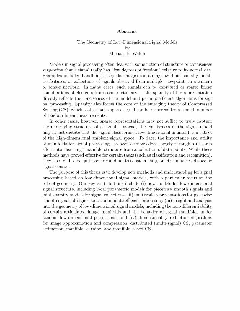
Abstract

The Geometry of Low-Dimensional Signal Modelsby

Michael B. Wakin

Models in signal processing often deal with some notion of structure or concisenesssuggesting that a signal really has “few degrees of freedom” relative to its actual size.Examples include: bandlimited signals, images containing low-dimensional geomet-ric features, or collections of signals observed from multiple viewpoints in a cameraor sensor network. In many cases, such signals can be expressed as sparse linearcombinations of elements from some dictionary — the sparsity of the representationdirectly reflects the conciseness of the model and permits efficient algorithms for sig-nal processing. Sparsity also forms the core of the emerging theory of CompressedSensing (CS), which states that a sparse signal can be recovered from a small numberof random linear measurements.

In other cases, however, sparse representations may not suffice to truly capturethe underlying structure of a signal. Instead, the conciseness of the signal modelmay in fact dictate that the signal class forms a low-dimensional manifold as a subsetof the high-dimensional ambient signal space. To date, the importance and utilityof manifolds for signal processing has been acknowledged largely through a researcheffort into “learning” manifold structure from a collection of data points. While thesemethods have proved effective for certain tasks (such as classification and recognition),they also tend to be quite generic and fail to consider the geometric nuances of specificsignal classes.

The purpose of this thesis is to develop new methods and understanding for signalprocessing based on low-dimensional signal models, with a particular focus on therole of geometry. Our key contributions include (i) new models for low-dimensionalsignal structure, including local parametric models for piecewise smooth signals andjoint sparsity models for signal collections; (ii) multiscale representations for piecewisesmooth signals designed to accommodate efficient processing; (iii) insight and analysisinto the geometry of low-dimensional signal models, including the non-differentiabilityof certain articulated image manifolds and the behavior of signal manifolds underrandom low-dimensional projections, and (iv) dimensionality reduction algorithmsfor image approximation and compression, distributed (multi-signal) CS, parameterestimation, manifold learning, and manifold-based CS.

Acknowledgements

The best part of graduate school has undoubtedly been getting to meet and workwith so many amazing people. It has been a great privilege to take part in severalexciting and intensive research projects, and I would like to thank my collaborators:Rich Baraniuk, Dror Baron, Rui Castro, Venkat Chandrasekaran, Hyeokho Choi,Albert Cohen, Mark Davenport, Ron DeVore, Dave Donoho, Marco Duarte, FelixFernandes, Jason Laska, Matthew Moravec, Mike Orchard, Justin Romberg, ChrisRozell, Shri Sarvotham, and Joel Tropp. This thesis owes a great deal to theircontributions, as I have also noted on the first page of several chapters.

I am also very grateful to my thesis committee for the many ways in which theycontributed to this work: to Mike Orchard for some very challenging but motivatingdiscussions; to Steve Cox for a terrific course introducing me to functional analysisback in my undergraduate days; to Ron DeVore for the time, energy, and humor hegenerously poured into his yearlong visit to Rice; to my “Dutch uncle” Dave Donohofor his patient but very helpful explanations and for strongly encouraging me to startearly on my thesis; and most of all to my advisor Rich Baraniuk for somehow providingme with the right mix of pressure and encouragement. Rich’s boundless energy hasbeen a true inspiration, and I thank him for the countless hours he enthusiasticallydevoted to helping me develop as a speaker, writer, and researcher.

Much of the inspiration for this work came during a Fall 2004 visit to the UCLAInstitute for Pure and Applied Mathematics (IPAM) for a program on MultiscaleGeometry and Analysis in High Dimensions. I am very grateful to the organizersof that program, particularly to Emmanuel Candes and Dave Donoho for severalenlightening conversations and to Peter Jones for having a good sense of humor.

At Rice, I could not have asked for a more fun or interesting group of people towork with: Becca, Chris, Clay, Courtney, Dror, Hyeokho, Ilan, Justin, Jyoti, Kadim,Laska, Lavu, Lexa, Liz, Marco, Mark, Matt G., Matthew M., Mike O., Mike R.,Mona, Neelsh, Prashant, Ray, Rich, Rob, Rui, Rutger, Ryan, Shri, Venkat, Vero,Vinay, William C., William M., and many more. Thank you all for making DuncanHall a place I truly enjoyed coming to work. I will fondly remember our favoritepastimes: long lunchtime conversations, Friday afternoons at Valhalla, waiting forRich to show up at meetings, etc.

Finally, thank you to all of my other friends and family who helped me make itthis far, providing critical encouragement, support, and distractions when I neededthem most: Mom, Dad, Larry, Jackie, Jason, Katy, Denver, Nasos, Dave, Alex, Clay,Sean, Megan, many good friends from The MOB, and everyone else who helped mealong the way. Thank you again.

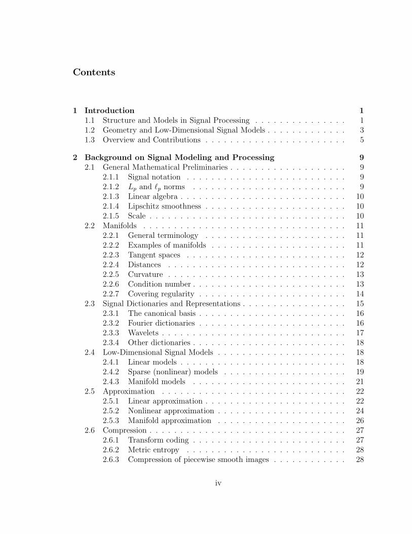
Contents

1 Introduction 11.1 Structure and Models in Signal Processing . . . . . . . . . . . . . . . 11.2 Geometry and Low-Dimensional Signal Models . . . . . . . . . . . . . 31.3 Overview and Contributions . . . . . . . . . . . . . . . . . . . . . . . 5

2 Background on Signal Modeling and Processing 92.1 General Mathematical Preliminaries . . . . . . . . . . . . . . . . . . . 9

2.1.1 Signal notation . . . . . . . . . . . . . . . . . . . . . . . . . . 92.1.2 Lp and `p norms . . . . . . . . . . . . . . . . . . . . . . . . . 92.1.3 Linear algebra . . . . . . . . . . . . . . . . . . . . . . . . . . . 102.1.4 Lipschitz smoothness . . . . . . . . . . . . . . . . . . . . . . . 102.1.5 Scale . . . . . . . . . . . . . . . . . . . . . . . . . . . . . . . . 10

2.2 Manifolds . . . . . . . . . . . . . . . . . . . . . . . . . . . . . . . . . 112.2.1 General terminology . . . . . . . . . . . . . . . . . . . . . . . 112.2.2 Examples of manifolds . . . . . . . . . . . . . . . . . . . . . . 112.2.3 Tangent spaces . . . . . . . . . . . . . . . . . . . . . . . . . . 122.2.4 Distances . . . . . . . . . . . . . . . . . . . . . . . . . . . . . 122.2.5 Curvature . . . . . . . . . . . . . . . . . . . . . . . . . . . . . 132.2.6 Condition number . . . . . . . . . . . . . . . . . . . . . . . . . 132.2.7 Covering regularity . . . . . . . . . . . . . . . . . . . . . . . . 14

2.3 Signal Dictionaries and Representations . . . . . . . . . . . . . . . . . 152.3.1 The canonical basis . . . . . . . . . . . . . . . . . . . . . . . . 162.3.2 Fourier dictionaries . . . . . . . . . . . . . . . . . . . . . . . . 162.3.3 Wavelets . . . . . . . . . . . . . . . . . . . . . . . . . . . . . . 172.3.4 Other dictionaries . . . . . . . . . . . . . . . . . . . . . . . . . 18

2.4 Low-Dimensional Signal Models . . . . . . . . . . . . . . . . . . . . . 182.4.1 Linear models . . . . . . . . . . . . . . . . . . . . . . . . . . . 182.4.2 Sparse (nonlinear) models . . . . . . . . . . . . . . . . . . . . 192.4.3 Manifold models . . . . . . . . . . . . . . . . . . . . . . . . . 21

2.5 Approximation . . . . . . . . . . . . . . . . . . . . . . . . . . . . . . 222.5.1 Linear approximation . . . . . . . . . . . . . . . . . . . . . . . 222.5.2 Nonlinear approximation . . . . . . . . . . . . . . . . . . . . . 242.5.3 Manifold approximation . . . . . . . . . . . . . . . . . . . . . 26

2.6 Compression . . . . . . . . . . . . . . . . . . . . . . . . . . . . . . . . 272.6.1 Transform coding . . . . . . . . . . . . . . . . . . . . . . . . . 272.6.2 Metric entropy . . . . . . . . . . . . . . . . . . . . . . . . . . 282.6.3 Compression of piecewise smooth images . . . . . . . . . . . . 28

iv

2.7 Dimensionality Reduction . . . . . . . . . . . . . . . . . . . . . . . . 292.7.1 Manifold learning . . . . . . . . . . . . . . . . . . . . . . . . . 302.7.2 The Johnson-Lindenstrauss lemma . . . . . . . . . . . . . . . 31

2.8 Compressed Sensing . . . . . . . . . . . . . . . . . . . . . . . . . . . 322.8.1 Motivation . . . . . . . . . . . . . . . . . . . . . . . . . . . . . 332.8.2 Incoherent projections . . . . . . . . . . . . . . . . . . . . . . 332.8.3 Methods for signal recovery . . . . . . . . . . . . . . . . . . . 342.8.4 Impact and applications . . . . . . . . . . . . . . . . . . . . . 362.8.5 The geometry of Compressed Sensing . . . . . . . . . . . . . . 372.8.6 Connections with dimensionality reduction . . . . . . . . . . . 38

3 Parametric Representation and Compression of Multi-DimensionalPiecewise Functions 393.1 Function Classes and Performance Bounds . . . . . . . . . . . . . . . 40

3.1.1 Multi-dimensional signal models . . . . . . . . . . . . . . . . . 403.1.2 Optimal approximation and compression rates . . . . . . . . . 423.1.3 “Oracle” coders and their limitations . . . . . . . . . . . . . . 44

3.2 The Surflet Dictionary . . . . . . . . . . . . . . . . . . . . . . . . . . 453.2.1 Motivation — Taylor’s theorem . . . . . . . . . . . . . . . . . 453.2.2 Definition . . . . . . . . . . . . . . . . . . . . . . . . . . . . . 463.2.3 Quantization . . . . . . . . . . . . . . . . . . . . . . . . . . . 47

3.3 Approximation and Compression of Piecewise Constant Functions . . 473.3.1 Overview . . . . . . . . . . . . . . . . . . . . . . . . . . . . . 473.3.2 Surflet selection . . . . . . . . . . . . . . . . . . . . . . . . . . 483.3.3 Tree-based surflet approximations . . . . . . . . . . . . . . . . 503.3.4 Leaf encoding . . . . . . . . . . . . . . . . . . . . . . . . . . . 513.3.5 Top-down predictive encoding . . . . . . . . . . . . . . . . . . 513.3.6 Extensions to broader function classes . . . . . . . . . . . . . 52

3.4 Approximation and Compression of Piecewise Smooth Functions . . . 543.4.1 Motivation . . . . . . . . . . . . . . . . . . . . . . . . . . . . . 543.4.2 Surfprints . . . . . . . . . . . . . . . . . . . . . . . . . . . . . 553.4.3 Vanishing moments and polynomial degrees . . . . . . . . . . 563.4.4 Quantization . . . . . . . . . . . . . . . . . . . . . . . . . . . 573.4.5 Surfprint-based approximation . . . . . . . . . . . . . . . . . . 583.4.6 Encoding a surfprint/wavelet approximation . . . . . . . . . . 59

3.5 Extensions to Discrete Data . . . . . . . . . . . . . . . . . . . . . . . 603.5.1 Overview . . . . . . . . . . . . . . . . . . . . . . . . . . . . . 603.5.2 Representing and encoding elements of FC(P,Hd) . . . . . . . 60

3.5.3 Representing and encoding elements of FS(P,Hd, Hs) . . . . . 623.5.4 Discretization effects and varying sampling rates . . . . . . . . 633.5.5 Simulation results . . . . . . . . . . . . . . . . . . . . . . . . . 64

v

4 The Multiscale Structure of Non-Differentiable Image Manifolds 704.1 Image Appearance Manifolds (IAMs) . . . . . . . . . . . . . . . . . . 71

4.1.1 Articulations in the image plane . . . . . . . . . . . . . . . . . 724.1.2 Articulations of 3-D objects . . . . . . . . . . . . . . . . . . . 73

4.2 Non-Differentiability from Edge Migration . . . . . . . . . . . . . . . 734.2.1 The problem . . . . . . . . . . . . . . . . . . . . . . . . . . . . 734.2.2 Approximate tangent planes via local PCA . . . . . . . . . . . 744.2.3 Approximate tangent planes via regularization . . . . . . . . . 754.2.4 Regularized tangent images . . . . . . . . . . . . . . . . . . . 76

4.3 Multiscale Twisting of IAMs . . . . . . . . . . . . . . . . . . . . . . . 774.3.1 Tangent bases for translating disk IAM . . . . . . . . . . . . . 774.3.2 Inter-scale twist angle . . . . . . . . . . . . . . . . . . . . . . 784.3.3 Intra-scale twist angle . . . . . . . . . . . . . . . . . . . . . . 794.3.4 Sampling . . . . . . . . . . . . . . . . . . . . . . . . . . . . . 80

4.4 Non-Differentiability from Edge Occlusion . . . . . . . . . . . . . . . 804.4.1 Articulations in the image plane . . . . . . . . . . . . . . . . . 814.4.2 3-D articulations . . . . . . . . . . . . . . . . . . . . . . . . . 82

4.5 Application: High-Resolution Parameter Estimation . . . . . . . . . . 834.5.1 The problem . . . . . . . . . . . . . . . . . . . . . . . . . . . . 834.5.2 Multiscale Newton algorithm . . . . . . . . . . . . . . . . . . 844.5.3 Examples . . . . . . . . . . . . . . . . . . . . . . . . . . . . . 864.5.4 Related work . . . . . . . . . . . . . . . . . . . . . . . . . . . 89

5 Joint Sparsity Models for Multi-Signal Compressed Sensing 915.1 Joint Sparsity Models . . . . . . . . . . . . . . . . . . . . . . . . . . . 92

5.1.1 JSM-1: Sparse common component + innovations . . . . . . . 935.1.2 JSM-2: Common sparse supports . . . . . . . . . . . . . . . . 935.1.3 JSM-3: Nonsparse common component + sparse innovations . 945.1.4 Refinements and extensions . . . . . . . . . . . . . . . . . . . 95

5.2 Recovery Strategies for Sparse Common Component + InnovationsModel (JSM-1) . . . . . . . . . . . . . . . . . . . . . . . . . . . . . . 95

5.3 Recovery Strategies for Common Sparse Supports Model (JSM-2) . . 975.3.1 Recovery via Trivial Pursuit . . . . . . . . . . . . . . . . . . . 985.3.2 Recovery via iterative greedy pursuit . . . . . . . . . . . . . . 995.3.3 Simulations for JSM-2 . . . . . . . . . . . . . . . . . . . . . . 102

5.4 Recovery Strategies for Nonsparse Common Component + Sparse In-novations Model (JSM-3) . . . . . . . . . . . . . . . . . . . . . . . . . 1025.4.1 Recovery via Transpose Estimation of Common Component . 1035.4.2 Recovery via Alternating Common and Innovation Estimation 1055.4.3 Simulations for JSM-3 . . . . . . . . . . . . . . . . . . . . . . 106

vi

6 Random Projections of Signal Manifolds 1096.1 Manifold Embeddings under Random Projections . . . . . . . . . . . 110

6.1.1 Inspiration — Whitney’s Embedding Theorem . . . . . . . . . 1106.1.2 Visualization . . . . . . . . . . . . . . . . . . . . . . . . . . . 1106.1.3 A geometric connection with Compressed Sensing . . . . . . . 1106.1.4 Stable embeddings . . . . . . . . . . . . . . . . . . . . . . . . 112

6.2 Applications in Compressed Sensing . . . . . . . . . . . . . . . . . . . 1136.2.1 Methods for signal recovery . . . . . . . . . . . . . . . . . . . 1146.2.2 Measurements . . . . . . . . . . . . . . . . . . . . . . . . . . . 1146.2.3 Stable recovery . . . . . . . . . . . . . . . . . . . . . . . . . . 1156.2.4 Basic examples . . . . . . . . . . . . . . . . . . . . . . . . . . 1166.2.5 Non-differentiable manifolds . . . . . . . . . . . . . . . . . . . 1206.2.6 Advanced models for signal recovery . . . . . . . . . . . . . . 123

6.3 Applications in Manifold Learning . . . . . . . . . . . . . . . . . . . . 1256.3.1 Manifold learning in RM . . . . . . . . . . . . . . . . . . . . . 1266.3.2 Experiments . . . . . . . . . . . . . . . . . . . . . . . . . . . . 127

7 Conclusions 1297.1 Models and Representations . . . . . . . . . . . . . . . . . . . . . . . 129

7.1.1 Approximation and compression . . . . . . . . . . . . . . . . . 1297.1.2 Joint sparsity models . . . . . . . . . . . . . . . . . . . . . . . 1317.1.3 Compressed Sensing . . . . . . . . . . . . . . . . . . . . . . . 131

7.2 Algorithms . . . . . . . . . . . . . . . . . . . . . . . . . . . . . . . . . 1327.2.1 Parameter estimation . . . . . . . . . . . . . . . . . . . . . . . 1327.2.2 Distributed Compressed Sensing . . . . . . . . . . . . . . . . . 132

7.3 Future Applications in Multi-Signal Processing . . . . . . . . . . . . . 132

A Proof of Theorem 2.1 136

B Proof of Theorem 5.3 138

C Proof of Theorem 6.2 140C.1 Preliminaries . . . . . . . . . . . . . . . . . . . . . . . . . . . . . . . 140C.2 Sampling the Manifold . . . . . . . . . . . . . . . . . . . . . . . . . . 141C.3 Tangent Planes at the Anchor Points . . . . . . . . . . . . . . . . . . 141C.4 Tangent Planes at Arbitrary Points on the Manifold . . . . . . . . . . 142C.5 Differences Between Nearby Points on the Manifold . . . . . . . . . . 142C.6 Differences Between Distant Points on the Manifold . . . . . . . . . . 144C.7 Synthesis . . . . . . . . . . . . . . . . . . . . . . . . . . . . . . . . . . 148

D Proof of Corollary 6.1 152

E Proof of Theorem 6.3 153

vii

List of Figures

1.1 Peppers test image and its wavelet coefficients. . . . . . . . . . . . . . 21.2 Four images of a rotating cube, corresponding to points on a non-

differentiable Image Appearance Manifold (IAM). . . . . . . . . . . . 3

2.1 Dyadic partitioning of the unit square at scales j = 0, 1, 2. . . . . . . 112.2 Charting the circle as a manifold. . . . . . . . . . . . . . . . . . . . . 122.3 A simple, redundant frame Ψ containing three vectors that span R2. . 162.4 Simple models for signals in R2. . . . . . . . . . . . . . . . . . . . . . 192.5 Approximating a signal x ∈ R2 with an `2 error criterion. . . . . . . . 23

3.1 Example piecewise constant and piecewise smooth functions. . . . . . 413.2 Example surflets. . . . . . . . . . . . . . . . . . . . . . . . . . . . . . 473.3 Example surflet tilings. . . . . . . . . . . . . . . . . . . . . . . . . . . 483.4 Example surflet and the corresponding surfprint. . . . . . . . . . . . . 553.5 Coding experiment for first 2-D piecewise constant test function. . . . 653.6 Coding experiment for second 2-D piecewise constant test function. . 663.7 Comparison of pruned surflet tilings using two surflet dictionaries. . . 673.8 Coding experiment for first 3-D piecewise constant test function. . . . 673.9 Volumetric slices of 3-D coded functions. . . . . . . . . . . . . . . . . 683.10 Coding experiment for second 3-D piecewise constant test function. . 69

4.1 Simple image articulation models. . . . . . . . . . . . . . . . . . . . . 724.2 Tangent plane basis vectors of the translating disk IAM. . . . . . . . 754.3 Intra-scale twist angles for translating disk. . . . . . . . . . . . . . . . 814.4 Changing tangent images for translating square before and after occlu-

sion. . . . . . . . . . . . . . . . . . . . . . . . . . . . . . . . . . . . . 814.5 Occlusion-based non-differentiability. . . . . . . . . . . . . . . . . . . 834.6 Multiscale estimation of translation parameters for observed disk image. 874.7 Multiscale estimation of translation parameters for observed disk image

with noise. . . . . . . . . . . . . . . . . . . . . . . . . . . . . . . . . . 874.8 Multiscale estimation of articulation parameters for ellipse. . . . . . . 884.9 Multiscale estimation of articulation parameters for 3-D icosahedron. 89

5.1 Converse bounds and achievable measurement rates for J = 2 signalswith common sparse component and sparse innovations (JSM-1). . . . 97

5.2 Reconstructing a signal ensemble with common sparse component andsparse innovations (JSM-1). . . . . . . . . . . . . . . . . . . . . . . . 98

5.3 Reconstruction using TP for JSM-2. . . . . . . . . . . . . . . . . . . . 1005.4 Reconstructing a signal ensemble with common sparse supports (JSM-2).103

viii

5.5 Reconstructing a signal ensemble with nonsparse common componentand sparse innovations (JSM-3) using ACIE. . . . . . . . . . . . . . . 108

6.1 Example random projections of 1-D manifolds. . . . . . . . . . . . . . 1116.2 Recovery of Gaussian bump parameters from random projections. . . 1176.3 Recovery of chirp parameters from random projections. . . . . . . . . 1186.4 Recovery of edge position from random projections. . . . . . . . . . . 1196.5 Edge position estimates from random projections of Peppers test image.1206.6 Recovery of ellipse parameters from multiscale random projections. . 1226.7 Multiscale random projection vectors. . . . . . . . . . . . . . . . . . . 1226.8 Noiselets. . . . . . . . . . . . . . . . . . . . . . . . . . . . . . . . . . 1236.9 Iterative recovery of multiple wedgelet parameters from random pro-

jections. . . . . . . . . . . . . . . . . . . . . . . . . . . . . . . . . . . 1246.10 Multiscale recovery of multiple wedgelet parameters from random pro-

jections. . . . . . . . . . . . . . . . . . . . . . . . . . . . . . . . . . . 1256.11 Setup for manifold learning experiment. . . . . . . . . . . . . . . . . . 1276.12 Manifold learning experiment in native high-dimensional space. . . . 1276.13 Manifold learning experiment using random projections. . . . . . . . 128

7.1 Comparison of wedgelet and barlet coding. . . . . . . . . . . . . . . . 1307.2 Recovering a 1-D signal X from random projections of known and

unknown delays of X. . . . . . . . . . . . . . . . . . . . . . . . . . . 134

ix

List of Tables

3.1 Surflet dictionary size at each scale. . . . . . . . . . . . . . . . . . . . 66

4.1 Estimation errors of Multiscale Newton iterations, translating disk, nonoise. . . . . . . . . . . . . . . . . . . . . . . . . . . . . . . . . . . . . 85

4.2 Estimation errors of Multiscale Newton iterations, translating disk,with noise. . . . . . . . . . . . . . . . . . . . . . . . . . . . . . . . . . 85

4.3 Estimation errors after Multiscale Newton iterations, ellipse. . . . . . 864.4 Estimation errors after Multiscale Newton iterations, 3-D icosahedron. 86

x

Chapter 1Introduction

1.1 Structure and Models in Signal Processing

Signal processing represents one of the primary interfaces of mathematics andscience. The abilities to efficiently and accurately measure, process, understand,quantify, compress, and communicate data and information rely both on accuratemodels for the situation at hand and on novel techniques inspired by the underlyingmathematics. The tools and algorithms that have emerged from such insights havehad far-reaching impacts, helping to revolutionize fields from communications [1] andentertainment [2] to biology [3] and medicine [4].

In characterizing a given problem, one is often able to specify a model for thesignals to be processed. This model may distinguish (either statistically or determin-istically) classes of interesting signals from uninteresting ones, typical signals fromanomalies, information from noise, etc. The model can also have a fundamental im-pact on the design and performance of signal processing tools and algorithms. As asimple example, one common assumption is that the signals to be processed are ban-dlimited, in which case each signal can be written as a different linear combinationof low-frequency sinusoids. Based on this assumption, then, the Shannon/Nyquistsampling theorem [5] specifies a minimal sampling rate for preserving the signal in-formation; this powerful result forms the core of modern Digital Signal Processing(DSP).

Like the assumption of bandlimitedness, models in signal processing often dealwith some notion of structure, constraint, or conciseness. Roughly speaking, one oftenbelieves that a signal has “few degrees of freedom” relative to the size of the signal.This can be caused, for example, by a physical system having few parameters, a limitto the information encoded in a signal, or an oversampling relative to the informationcontent of a signal. This notion of conciseness is a very powerful assumption, and itsuggests the potential for dramatic gains via algorithms that capture and exploit thetrue underlying structure of the signal.

To give a more concrete example, one popular generalization1 of the bandlimitedmodel in signal processing is sparsity, in which each signal is well-approximated asa small linear combination of elements from some basis or dictionary, but the choiceof elements may vary from signal to signal [6, 7]. In the frequency domain, a sparsemodel would suggest that each signal consists of just a few sinusoids, whose ampli-

1Or refinement, depending on one’s perspective.

1

(a) (b)

Figure 1.1: (a) Peppers test image. (b) Wavelet coefficient magnitudes in coarse-to-finescales of analysis (vertical subbands shown). At each scale, the relatively few significantwavelet coefficients tend to cluster around the edges of the objects in the image. Thismakes possible a variety of effective models for capturing intra- and inter-scale dependenciesamong the wavelet coefficients but also implies that the locations of significant coefficientswill change from image to image.

tudes, phases, and frequencies are variable. (A recording of a musical performance,for example, might be sparse in a dictionary containing sinusoids of limited dura-tion.) Sparsity has also been exploited in fields such as image processing, where themultiscale wavelet transform [5] permits concise, efficiently computable descriptionsof images (see Figure 1.1). In a nutshell, wavelets provide a sparse representationfor natural images because large smooth image regions require very few wavelets todescribe; only the abrupt edges separating smooth regions require large (significant)wavelet coefficients, and those regions occupy a relatively small total area of the im-age. The key phenomenon to note, however, is that the locations of these significantcoefficients may change from image to image.

Sparse representations have proven themselves as a powerful tool for capturingconcise signal structure and have led to fast, effective algorithms for solving keyproblems in signal processing. Wavelets form the core of many state-of-the art meth-ods for data compression and noise removal [8–12] — the multiscale structure of thewavelet transform suggests a top-down tree structure that is particularly effectivefor computation and modeling. Curvelets have also recently emerged as a multi-scale dictionary better suited to edge-like phenomena in two-dimensional (2-D) andthree-dimensional (3-D) signals [13–15] and have proven effective, for example, insolving inverse problems for seismic data processing. Inspired by successes such asthese, research continues in developing novel sparse dictionaries that are adapted tobroader families of signal classes and, again, that are amenable to fast algorithms(often through a multiscale structure).

As we have stated, the notion that many signals have sparse structure is widespreadin signal processing and eminently useful. However, sparsity itself can sometimes bea rather restrictive assumption; there are many other interesting and important no-tions of concise signal structure that may not give rise to representations that aresparse in the conventional sense. Such notions often arise in cases where (i) a smallcollection of parameters can be identified that carry the relevant information about

2

Figure 1.2: Four 256×256 = 65536-pixel images of an identical cube, differing only in theposition of the cube (10 degrees of rotation between each frame). As the cube rotates, theimages change (edges move, shadings differ, etc.), and the resulting images trace out a pathon a low-dimensional manifold within the high-dimensional ambient signal space R65536. Aswe discuss in Chapter 4, this manifold is in fact non-differentiable.

a signal and (ii) the signal changes as a function of these parameters. Some simpleexplicit examples include: the time delay of a 1-D signal (parametrized by 1 vari-able for translation), the configuration of a straight edge in a local image segment(2 parameters: slope and offset), the position of a camera photographing a scene(∼6 parameters), the relative placement of objects in a scene, the duration and chirprate of a radar pulse, or other parameters governing the output of some articulatedphysical system [16–19].

In some cases, these parameters may suffice to completely describe the signal; inother cases they may merely serve to distinguish it from other, related signals in theclass. (See, for example, the images in Figure 1.2.) The key is that, for a particularproblem, the relevant information about a signal can often be summarized in a smallnumber of variables (the “degrees of freedom”). While the signal may also happen tohave a sparse representation in some dictionary (such as the wavelet transform of animage of a straight edge), this sparsity will rarely reflect the true “information level”of the signal. This motivates a search for novel signal processing representations andalgorithms that better exploit the conciseness of such signal models, including caseswhere the parametric model is only an approximation or where the parametric modelis actually unknown.

1.2 Geometry and Low-Dimensional Signal Models

As we have discussed, models play a critical role in signal processing. In a verybroad sense, a model can be thought of as an answer to the question: “What are thesignals of interest?” Based on our understanding of this model, our goal is to developefficient tools, representations, algorithms, and so on.

As an inspiration for developing these solutions, we believe that significant math-ematical insight can often be gained by asking a related geometric question: “Whereare the signals of interest?” That is, where do signals in the model class reside as a

3

subset of the ambient signal space (e.g., RN for real-valued discrete length-N signals)?Indeed, as we will see, many of the concise signal models discussed in Section 1.1 actu-ally translate to low-dimensional structures within the high-dimensional signal space;again, the low dimension of these structures suggests the potential for fast, powerfulalgorithms. By studying and understanding the geometry of these low-dimensionalstructures, we hope to identify new challenges in signal processing and to discovernew solutions.

Returning to some specific examples, bandlimited signals live on a low-dimensionallinear subspace of the ambient signal space (see Section 2.4.1); indeed, the very word“linear” immediately evokes a geometric understanding. It follows immediately, then,that tasks such as optimally removing noise from a signal (in a least-squares sense)would simply involve orthogonal projection onto this subspace.

Sparse signals, on the other hand, live near a nonlinear set that is a union of suchlow-dimensional subspaces. Again, this geometry plays a critical role in the signalprocessing; Chapter 2 discusses in depth the implications for tasks such as approxi-mation and compression. One of the most surprising implications of the nonlinear,low-dimensional geometry of sparse signal sets comes from the recent theory of Com-pressed Sensing (CS) [20, 21]. The CS theory states that a length-N signal that isK-sparse (it can be written as a sum of K basis elements) can be reconstructed fromonly cK nonadaptive linear projections onto a second basis that is incoherent withthe first, where typically c ≈ 3 or 4. (A random basis provides such incoherence withvery high probability.) This has many promising applications in signal acquisition,compression, medical imaging, and sensor networks [22–33]. A key point is that theCS theory relies heavily on geometric notions such as the n-widths of `p balls and theproperties of randomly projected polytopes [20,21,23,34–40] (see Section 2.8.5).

In more general cases where one has a concise model for signal structure, theresulting signal class often manifests itself as a low-dimensional, nonlinear manifoldembedded in the high-dimensional signal space.2 This is the case, in particular, forparametric signal models; as discussed in Section 2.4.3, the dimension of the manifoldwill match the dimension of the underlying parameter (the number of degrees offreedom). More generally, however, manifolds have also been discovered as usefulapproximations for signal classes not obeying an explicit parametric model. Examplesinclude the output of dynamical systems having low-dimensional attractors [41,42] orcollections of images such as faces or handwritten digits [43].

Naturally, the geometry of signal manifolds will also have a critical impact onthe performance of signal processing methods. To date, the importance and utilityof manifolds for signal processing has been acknowledged largely through a researcheffort into “learning” manifold structure from a collection of data points, typicallyby constructing “dimensionality reducing” mappings to lower-dimensional space that

2A manifold can be thought of as a low-dimensional, nonlinear “surface” within the high-dimensional signal space; Section 2.2 gives a more precise definition. Note that the linear subspaceand “union of subspaces” models are essentially special cases of such manifold structure.

4

reveal the locally Euclidean nature of the manifold or by building functions on thedata that reveal its metric structure [41–54] (see also Section 2.7.1). While thesemethods have proven effective for certain tasks (such as classification and recogni-tion), they also tend to be quite generic. Due to the wide variety of situations inwhich signal manifolds may arise, however, different signal classes may have differentgeometric nuances that deserve special attention. Relatively few studies have consid-ered the geometry of specific classes of signals; important exceptions include the workof Lu [55], who empirically studied properties such as the dimension and curvatureof image manifolds, Donoho and Grimes [16], who examined the metric structure ofarticulated image manifolds, and Mumford et al. [56], who used manifolds to modelsets of shapes. In general, we feel that the incorporation of the manifold viewpointinto signal processing is only beginning, and more careful studies will both advanceour understanding and inspire new solutions.

1.3 Overview and Contributions

The purpose of this thesis is to develop new methods and understanding for signalprocessing based on low-dimensional signal models, with a particular focus on the roleof geometry. To guide our study, we consider two primary application areas:

1. Image processing, a research area of broad importance in which concise signalmodels abound (thanks to the articulations of objects in a scene, the regularityof smooth regions, and the 1-D geometry of edges), and

2. Compressed Sensing, a nascent but markedly geometric theory with great promisefor applications in signal acquisition, compression, medical imaging, and sensornetworks.

Our key contributions include new:

• concise signal models that generalize the conventional notion of sparsity;

• multiscale representations for sparse approximation and compression;

• insight and analysis into the geometry of low-dimensional signal models basedon concepts in differential geometry and differential topology; and

• algorithms for parameter estimation and dimensionality reduction inspired bythe underlying manifold structure.

We outline these contributions chapter-by-chapter.We begin in Chapter 2 with a background discussion of low-dimensional signal

models. After a short list of mathematical preliminaries and notation, including abrief introduction to manifolds, we discuss the role of signal dictionaries and rep-resentations, the geometry of linear, sparse, and manifold-based signal models, and

5

the implications in problems such as approximation and compression. We also dis-cuss more advanced techniques in dimensionality reduction, manifold learning, andCompressed Sensing.

In Chapter 3 we consider the task of approximating and compressing two modelclasses of functions for which traditional harmonic dictionaries fail to provide sparserepresentations. However, the model itself dictates a low-dimensional structure tothe signals, which we capture using a novel parametric multiscale dictionary. Thefunctions we consider are both highly relevant in signal processing and highly struc-tured. In particular, we consider piecewise constant signals in P dimensions where asmooth (P − 1)-dimensional discontinuity separates the two constant regions, and wealso consider the extension of this class to piecewise smooth signals, where a smooth(P − 1)-dimensional discontinuity separates two smooth regions. These signal classesprovide basic models, for example, for images containing edges, video sequences ofmoving objects, or seismic data containing geological horizons. Despite the under-lying (indeed, low-dimensional) structure in each of these classes, classical harmonicdictionaries fail to provide sparse representations for such signals. The problem comesfrom the (P − 1)-dimensional discontinuity, whose smooth geometric structure is notcaptured by local isotropic representations such as wavelets.

As a remedy, we propose a multiscale dictionary consisting of local parametricatoms called surflets, each a piecewise constant function with a (tunable) polynomialdiscontinuity separating the two constant regions. Our surflet dictionary falls outsidethe traditional realm of bases and frames (where approximations are assembled as lin-ear combinations of atoms from the dictionary). Rather our scheme is perhaps betterviewed as a “geometric tiling,” where precisely one atom from the dictionary is usedto describe the signal at each part of the domain (these atoms “tile” together to coverthe domain). We discuss multiscale (top-down, tree-based) schemes for assemblingand encoding surflet representations, and we prove that such schemes attain optimalasymptotic approximation and compression performance on our piecewise constantfunction classes. We also discuss techniques for interfacing surflets with waveletsfor representing more general classes of functions. The resulting dictionary, whichwe term surfprints, attains near-optimal asymptotic approximation and compressionperformance on our piecewise smooth function classes.

In Chapter 4 we study the geometry of signal manifolds in more detail, particu-larly in the case of parametrized image manifolds (such as the 2-D surflet manifold).We call these Image Appearance Manifolds (IAMs) and let θ denote the parametercontrolling the image formation. Our work builds upon a surprising realization [16]:IAMs of continuous images having sharp edges that move as a function of θ arenowhere differentiable. This presents an immediate challenge for signal processing al-gorithms that might assume differentiability or smoothness of such manifolds. UsingNewton’s method, for example, to estimate the parameter θ for an unlabeled image,would require successive projections onto tangent spaces of the manifold. Becausethe manifold is not differentiable, however, these tangents do not exist.

6

Although these IAMs lack differentiability, we identify a multiscale collection oftangent spaces to the manifold, each one associated with both a location on themanifold and scale of analysis; this multiscale structure can be accessed simply byregularizing the images. Based on this multiscale perspective, we propose a Multi-scale Newton algorithm to solve the parameter estimation problem. We also reveal asecond, more localized kind of IAM non-differentiability caused by sudden occlusionsof edges at special values of θ. This type of phenomenon has its own implications inthe signal processing and requires a special vigilance; it is not alleviated by merelyregularizing the images.

In Chapter 5 we consider another novel modeling perspective, as we turn our at-tention toward a suite of signal models designed for simultaneous modeling of multiplesignals that have a shared concise structure. Our primary motivation for introducingthese models is to extend the CS theory and methods to a multi-signal setting —while CS appears promising for applications such as sensor networks, at present it istailored only for the sensing of a single sparse signal.

We introduce a new theory for Distributed Compressed Sensing (DCS) that enablesnew distributed coding algorithms that exploit both intra- and inter-signal correlationstructures. In a typical DCS scenario, a number of sensors measure signals that areeach individually sparse in some basis and also correlated from sensor to sensor. Eachsensor independently encodes its signal by projecting it onto another, incoherent basis(such as a random one) and then transmits just a few of the resulting coefficients to asingle collection point. Under the right conditions, a decoder at the collection pointcan reconstruct each of the signals precisely.

The DCS theory rests on a concept that we term the joint sparsity of a signalensemble. We study in detail three simple models for jointly sparse signals, proposetractable algorithms for joint recovery of signal ensembles from incoherent projections,and characterize theoretically and empirically the number of measurements per sen-sor required for accurate reconstruction. While the sensors operate entirely withoutcollaboration, our simulations reveal that in practice the savings in the total numberof required measurements can be substantial over separate CS decoding, especiallywhen a majority of the sparsity is shared among the signals.

In Chapter 6, inspired again by a geometric perspective, we develop new theoryand methods for problems involving random projections for dimensionality reduc-tion. In particular, we consider embedding results previously applicable only to finitepoint clouds (the Johnson-Lindenstrauss lemma; see Section 2.7.2) or to sparse signalmodels (Compressed Sensing) and generalize these results to include manifold-basedsignal models. As our primary theoretical contribution (Theorem 6.2), we considerthe effect of a random projection operator on a smooth K-dimensional submanifoldof RN , establishing a sufficient number M of random projections to ensure a stableembedding. We explore a number of possible applications of this result, particularlyin CS, which we generalize beyond the recovery of sparse signals to include the recov-ery of manifold-modeled signals from small number of random projections. We also

7

discuss other possible applications in manifold learning and dimensionality reduction.We conclude in Chapter 7 with a final discussion and directions for future re-

search.

This thesis is a reflection of a series of intensive and inspiring collaborations.Where appropriate, the first page of each chapter includes a list of primary collabo-rators, who share the credit for this work.

8

Chapter 2Background on Signal Modeling and Processing

2.1 General Mathematical Preliminaries

2.1.1 Signal notation

We will treat signals as real- or complex-valued functions having domains thatare either discrete (and finite) or continuous (and either compact or infinite). Eachof these assumptions will be made clear in the particular chapter or section. As ageneral rule, however, we will use x to denote a discrete signal in RN and f to denote afunction over a continuous domain D. We also commonly refer to these as discrete- orcontinuous-time signals, though the domain need not actually be temporal in nature.Additional chapter-specific conventions will be specified as necessary.

2.1.2 Lp and `p norms

As measures for signal energy, fidelity, or sparsity, we will often employ the Lp

and `p norms. For continuous-time functions, the Lp norm is defined as

‖f‖Lp(D) =

(∫

D|f |p)1/p

, p ∈ (0,∞),

and for discrete-time functions, the `p norm is defined as

‖x‖`p =

(∑N

i=1 |x(i)|p)1/p, p ∈ (0,∞),

maxi=1,...,N |x(i)|, p =∞,∑N

i=1 1x(i) 6=0, p = 0,

where 1 denotes the indicator function. (While we often refer to these measures as“norms,” they actually do not meet the technical criteria for norms when p < 1.)

The mean-square error (MSE) between two discrete-time signals x1, x2 ∈ RN

is given by 1N‖x1 − x2‖22. The peak signal-to-noise ratio (PSNR), another common

measure of distortion between two signals, derives directly from the MSE; assuminga maximum possible signal intensity of I, PSNR := 10 log10

I2

MSE.

9

2.1.3 Linear algebra

Let A be a real-valued M × N matrix. We denote the nullspace of A as N (A)(note that N (A) is a linear subspace of RN), and we denote the transpose of A asAT .

We call A an orthoprojector from RN to RM if it has orthonormal rows. Fromsuch a matrix we call A

TA the corresponding orthogonal projection operator onto the

M -dimensional subspace of RN spanned by the rows of A.

2.1.4 Lipschitz smoothness

We say a continuous-time function of D variables has smoothness of order H > 0,where H = r+ν, r is an integer, and ν ∈ (0, 1], if the following criteria are met [57,58]:

• All iterated partial derivatives with respect to the D directions up to order rexist and are continuous.

• All such partial derivatives of order r satisfy a Lipschitz condition of order ν(also known as a Holder condition).1

We will sometimes consider the space of smooth functions whose partial derivativesup to order r are bounded by some constant Ω. We denote the space of such boundedfunctions with bounded partial derivatives by CH , where this notation carries animplicit dependence on Ω. Observe that r = dH−1e, where d·e denotes rounding up.Also, when H is an integer CH includes as a subset the traditional space “CH” (theclass of functions that have H = r + 1 continuous partial derivatives).

2.1.5 Scale

We will frequently refer to a particular scale of analysis for a signal. Suppose ourfunctions f are defined over the continuous domain D = [0, 1]D. A dyadic hypercubeXj ⊆ [0, 1]D at scale j ∈ N is a domain that satisfies

Xj = [β12−j, (β1 + 1)2−j]× · · · × [βD2−j, (βD + 1)2−j]

with β1, β2, . . . , βD ∈ 0, 1, . . . , 2j − 1. We call Xj a dyadic interval when D = 1 ora dyadic square when D = 2 (see Figure 2.1). Note that Xj has sidelength 2−j.

For discrete-time functions the notion of scale is similar. We can imagine, forexample, a “voxelization” of the domain [0, 1]D (“pixelization” when D = 2), whereeach voxel has sidelength 2−B, B ∈ N, and it takes 2BD voxels to fill [0, 1]D. Therelevant scales of analysis for such a signal would simply be j = 0, 1, . . . , B, and eachdyadic hypercube Xj would refer to a collection of voxels.

1A function d ∈ Lip(ν) if |d(t1 + t2)− d(t1)| ≤ C‖t2‖ν for all D-dimensional vectors t1, t2.

10

j=0 j=1 j=2

1/41/21

Figure 2.1: Dyadic partitioning of the unit square at scales j = 0, 1, 2. The partitioninginduces a coarse-to-fine parent/child relationship that can be modeled using a tree structure.

2.2 Manifolds

We present here a minimal, introductory set of definitions and terminology fromdifferential geometry and topology, referring the reader to the introductory and clas-sical texts [59–62] for more depth and technical precision.

2.2.1 General terminology

A K-dimensional manifold M is a topological space2 that is locally homeomor-phic3 to RK [61]. This means that there exists an open cover of M with each suchopen set mapping homeomorphically to an open ball in RK . Each such open set,together with its mapping to RK is called a chart; the set of all charts of a manifoldis called an atlas.

The general definition of a manifold makes no reference to an ambient space inwhich the manifold lives. However, as we will often be making use of manifolds asmodels for sets of signals, it follows that such “signal manifolds” are actually subsetsof some larger space (for example, of L2(R) or RN). In general, we may think of aK-dimensional submanifold embedded in RN as a nonlinear, K-dimensional “surface”within RN .

2.2.2 Examples of manifolds

One of the simplest examples of a manifold is simply the circle in R2. A small,open-ended segment cut from the circle could be stretched out and associated withan open interval of the real line (see Figure 2.2). Hence, the circle is a 1-D manifold.

2A topological space is simply a set X, together with a collection T of subsets of X called opensets, such that: (i) the empty set belongs to T , (ii) X belongs to T , (iii) arbitrary unions of elementsof T belong to T , and (iv) finite intersections of elements of T belong to T .

3A homeomorphism is a function between two topological spaces that is one-to-one, onto, con-tinuous, and has a continuous inverse.

11

U U1 2ϕ 21ϕ

Figure 2.2: A circle is a manifold because there exists an open cover consisting of the setsU1, U2, which are mapped homeomorphically onto open intervals in the real line via thefunctions ϕ1, ϕ2. (It is not necessary that the intervals intersect in R.)

(We note that at least two charts are required to form an atlas for the circle, as theentire circle itself cannot be mapped homeomorphically to an open interval in R1.)

We refer the reader to [63] for an excellent overview of several manifolds withrelevance to signal processing, including the rotation group SO(3), which can be usedfor representing orientations of objects in 3-D space, and the Grassman manifoldG(K,N), which represents all K-dimensional subspaces of RN . (Without workingthrough the technicalities of the definition of a manifold, it is easy to see that bothtypes of data have a natural notion of neighborhood.)

2.2.3 Tangent spaces

A manifold is differentiable if, for any two charts whose open sets onM overlap,the composition of the corresponding homeomorphisms (from RK in one chart toMand back to RK in the other) is differentiable. (In our simple example, the circle is adifferentiable manifold.)

To each point x in a differentiable manifold, we may associate a K-dimensionaltangent space Tanx. For signal manifolds embedded in L2 or RN , it suffices to thinkof Tanx as the set of all directional derivatives of smooth paths on M through x.(Note that Tanx is a linear subspace and has its origin at 0, rather than at x.)

2.2.4 Distances

One is often interested in measuring distance along a manifold. For abstractdifferentiable manifolds, this can be accomplished by defining a Riemannian metricon the tangent spaces. A Riemannian metric is a collection of inner products 〈, 〉xdefined at each point x ∈M. The inner product gives a measure for the “length” ofa tangent, and one can then compute the length of a path on M by integrating itstangent lengths along the path.

For differentiable manifolds embedded in RN , the natural metric is the Euclideanmetric inherited from the ambient space. The length of a path γ : [0, 1] 7→ M can

12

then be computed simply using the limit

length(γ) = limj→∞

j∑

i=1

‖γ(i/j)− γ((i− 1)/j)‖2 .

The geodesic distance dM(x, y) between two points x, y ∈ M is then given by thelength of the shortest path γ onM joining x and y.

2.2.5 Curvature

Several notions of curvature also exist for manifolds. The curvature of a unit-speedpath in RN is simply given by its second derivative. More generally, for manifoldsembedded in RN , characterizations of curvature generally relate to the second deriva-tives of paths alongM (in particular, the components of the second derivatives thatare normal toM). Section 2.2.6 characterizes the notions of curvature and “twisting”of a manifold that will be most relevant to us.

2.2.6 Condition number

To give ourselves a firm footing for later analysis, we find it helpful assume acertain regularity to the manifold beyond mere differentiability. For this purpose, weadopt the condition number defined recently by Niyogi et al. [51].

Definition 2.1 [51] LetM be a compact submanifold of RN . The condition numberof M is defined as 1/τ , where τ is the largest number having the following property:The open normal bundle about M of radius r is imbedded in RN for all r < τ .

The open normal bundle of radius r at a point x ∈ M is simply the collection ofall vectors of length < r anchored at x and with direction orthogonal to Tanx.

In addition to controlling local properties (such as curvature) of the manifold,the condition number has a global effect as well, ensuring that the manifold is self-avoiding. These notions are made precise in several lemmata, which we will findhelpful for analysis and which we repeat below for completeness.

Lemma 2.1 [51] IfM is a submanifold of RN with condition number 1/τ , then thenorm of the second fundamental form is bounded by 1/τ in all directions.

This implies that unit-speed geodesic paths on M have curvature bounded by1/τ . The second lemma concerns the twisting of tangent spaces.

Lemma 2.2 [51] Let M be a submanifold of RN with condition number 1/τ . Letp, q ∈M be two points with geodesic distance given by dM(p, q). Let θ be the angle be-tween the tangent spaces Tanp and Tanq defined by cos(θ) = minu∈Tanp maxv∈Tanq |〈u, v〉|.Then cos(θ) > 1− 1

τdM(p, q).

13

The third lemma concerns self-avoidance ofM.

Lemma 2.3 [51] Let M be a submanifold of RN with condition number 1/τ . Letp, q ∈ M be two points such that ‖p− q‖2 = d. Then for all d ≤ τ/2, the geodesic

distance dM(p, q) is bounded by dM(p, q) ≤ τ − τ√

1− 2d/τ .

From Lemma 2.3 we have an immediate corollary.

Corollary 2.1 LetM be a submanifold of RN with condition number 1/τ . Let p, q ∈M be two points such that ‖p− q‖2 = d. If d ≤ τ/2, then d ≥ dM(p, q)− (dM(p,q))2

2τ.

2.2.7 Covering regularity

For future reference, we also introduce a notion of “geodesic covering regularity”for a manifold.

Definition 2.2 Let M be a compact submanifold of RN . Given T > 0, the geodesiccovering number G(T ) of M is defined as the smallest number such that there existsa set A of points, #A = G(T ), so that for all x ∈M,

mina∈A

dM(x, a) ≤ T.

Definition 2.3 Let M be a compact K-dimensional submanifold of RN having vol-ume V . We say that M has geodesic covering regularity R if

G(T ) ≤ RVKK/2

TK(2.1)

for all T > 0.

The volume referred to above is K-dimensional volume (also known as lengthwhen K = 1 or surface area when K = 2).

The geodesic covering regularity of a manifold is closely related to its ambientdistance-based covering number C(T ) [51]. In fact, for a manifold with conditionnumber 1/τ , we can make this connection explicit. Lemma 2.3 implies that for smalld, dM(p, q) ≤ τ − τ

√1− 2d/τ ≤ τ(1− (1− 2d/τ)) = 2d. This implies that G(T ) ≤

C(T/4) for small T . Pages 13–14 of [51] also establish that for small T , the ambientcovering number can be bounded by a packing number P (T ) of the manifold, from

14

which we conclude that

G(T ) ≤ C(T/4) ≤ P (T/8)

≤ V

cos(arcsin( T16τ

))Kvol(BKT/8)

≤ V · Γ(K/2 + 1)

(1− ( T16τ

)2)K/2πK/2(T/8)K

≤ Const · V KK/2

TK.

Although we point out this connection between the geodesic covering regularity andthe condition number, for future reference and flexibility we prefer to specify these asdistinct properties in our results in Chapter 6.

2.3 Signal Dictionaries and Representations

For a wide variety of signal processing applications (including analysis, compres-sion, noise removal, and so on) it is useful to consider the representation of a signalin terms of some dictionary [5]. In general, a dictionary Ψ is simply a collectionof elements drawn from the signal space whose linear combinations can be used torepresent or approximate signals.

Considering, for example, signals in RN , we may collect and represent the elementsof the dictionary Ψ as an N × Z matrix, which we also denote as Ψ. From thisdictionary, a signal x ∈ RN can be constructed as a linear combination of the elements(columns) of Ψ. We write

x = Ψα

for some α ∈ RZ . (For much of our notation in this section, we concentrate on signalsin RN , though the basic concepts translate to other vector spaces.)

Dictionaries appear in a variety of settings. The most common may be the basis,in which case Ψ has exactly N linearly independent columns, and each signal x hasa unique set of expansion coefficients α = Ψ−1x. The orthonormal basis (where thecolumns are normalized and orthogonal) is also of particular interest, as the uniqueset of expansion coefficients α = Ψ−1x = Ψ

Tx can be obtained as the inner products

of x against the columns of Ψ. That is, α(i) = 〈x, ψi〉 , i = 1, 2, . . . , N , which gives usthe expansion

x =N∑

i=1

〈x, ψi〉ψi.

We also have that ‖x‖22 =∑N

i=1 〈x, ψi〉2.Frames are another special type of dictionary [64]. A dictionary Ψ is a frame if

15

x(1)

x(2)

ψ ψ

ψ

23

1

Figure 2.3: A simple, redundant frame Ψ containing three vectors that span R2.

there exist numbers A and B, 0 < A ≤ B <∞ such that, for any signal x

A ‖x‖22 ≤∑

z

〈x, ψz〉2 ≤ B ‖x‖22 .

The elements of a frame may be linearly dependent in general (see Figure 2.3), andso there may exist many ways to express a particular signal among the dictionaryelements. However, frames do have a useful analysis/synthesis duality: for any frame

Ψ there exists a dual frame Ψ such that

x =∑

z

〈x, ψz〉 ψz =∑

z

⟨x, ψz

⟩ψz.

A frame is called tight if the frame bounds A and B are equal. Tight frames havethe special properties of (i) being their own dual frames (after a rescaling by 1/A)and (ii) preserving norms, i.e.,

∑Ni=1 〈x, ψi〉2 = A ‖x‖22. The remainder of this section

discusses several important dictionaries.

2.3.1 The canonical basis

The standard basis for representing a signal is the canonical (or “spike”) basis.In RN , this corresponds to a dictionary Ψ = IN (the N ×N identity matrix). Whenexpressed in the canonical basis, signals are often said to be in the “time domain.”

2.3.2 Fourier dictionaries

The frequency domain provides one alternative representation to the time domain.The Fourier series and discrete Fourier transform are obtained by letting Ψ containcomplex exponentials and allowing the expansion coefficients α to be complex as well.(Such a dictionary can be used to represent real or complex signals.) A related “har-monic” transform to express signals in RN is the discrete cosine transform (DCT), in

16

which Ψ contains real-valued, approximately sinusoidal functions and the coefficientsα are real-valued as well.

2.3.3 Wavelets

Closely related to the Fourier transform, wavelets provide a framework for local-ized harmonic analysis of a signal [5]. Elements of the discrete wavelet dictionaryare local, oscillatory functions concentrated approximately on dyadic supports andappear at a discrete collection of scales, locations, and (if the signal dimension D > 1)orientations.

The wavelet transform offers a multiscale decomposition of a function into a nestedsequence of scaling spaces V0 ⊂ V1 ⊂ · · · ⊂ Vj ⊂ · · · . Each scaling space is spannedby a discrete collection of dyadic translations of a lowpass scaling function ϕj. Thecollection of wavelets at a particular scale j spans the difference between adjacentscaling spaces Vj and Vj−1. (Each wavelet function at scale j is concentrated approx-imately on some dyadic hypercube Xj, and between scales, both the wavelets andscaling functions are “self-similar,” differing only by rescaling and dyadic dilation.)When D > 1, the difference spaces are partitioned into 2D − 1 distinct orientations(when D = 2 these correspond to vertical, horizontal, and diagonal directions). Thewavelet transform can be truncated at any scale j. We then let the basis Ψ consistof all scaling functions at scale j plus all wavelets at scales j and finer.

Wavelets are essentially bandpass functions that detect abrupt changes in a signal.The scale of a wavelet, which controls its support both in time and in frequency,also controls its sensitivity to changes in the signal. This is made more precise byconsidering the wavelet analysis of smooth signals. Wavelet are often characterizedby their number of vanishing moments; a wavelet basis function is said to have Hvanishing moments if it is orthogonal to (its inner product is zero against) any H-degree polynomial. Section 2.4.2 discusses further the wavelet analysis of smooth andpiecewise smooth signals.

The dyadic organization of the wavelet transform lends itself to a multiscale, tree-structured organization of the wavelet coefficients. Each “parent” function, concen-trated on a dyadic hypercube Xj of sidelength 2−j, has 2D “children” whose supportsare concentrated on the dyadic subdivisions of Xj. This relationship can be repre-sented in a top-down tree structure. Because the parent and children share a location,they will presumably measure related phenomena about the signal, and so in general,any patterns in their wavelet coefficients tend to be reflected in the connectivity ofthe tree structure.

In addition to their ease of modeling, wavelets are computationally attractive forsignal processing; using a filter bank, the wavelet transform of an N -voxel signal canbe computed in just O(N) operations.

17

2.3.4 Other dictionaries

A wide variety of other dictionaries have been proposed in signal processing andharmonic analysis. As one example, complex-valued wavelet transforms have provenuseful for image analysis and modeling [65–71], thanks to a phase component thatcaptures location information at each scale. Just a few of the other harmonic dic-tionaries popular in image processing include wavelet packets [5], Gabor atoms [5],curvelets [13,14], and contourlets [72,73], all of which involve various space-frequencypartitions. We mention additional dictionaries in Section 2.6, and we also discuss inChapter 3 alternative methods for signal representation such as tilings, where pre-cisely one atom from the dictionary is used to describe the signal at each part of thedomain (and these atoms “tile” together to cover the entire domain).

2.4 Low-Dimensional Signal Models

We now survey some common and important models in signal processing, eachof which involves some notion of conciseness to the signal structure. We see in eachcase that this conciseness gives rise to a low-dimensional geometry within the ambientsignal space.

2.4.1 Linear models

Some of the simplest models in signal processing correspond to linear subspaces ofthe ambient signal space. Bandlimited signals are one such example. Supposing, forexample, that a 2π-periodic signal f has Fourier transform F (ω) = 0 for |ω| > B, theShannon/Nyquist sampling theorem [5] states that such signals can be reconstructedfrom 2B samples. Because the space of B-bandlimited signals is closed under additionand scalar multiplication, it follows that the set of such signals forms a 2B-dimensionallinear subspace of L2([0, 2π)).

Linear signal models also appear in cases where a model dictates a linear constrainton a signal. Considering a discrete length-N signal x, for example, such a constraintcan be written in matrix form as

Ax = 0

for some M × N matrix A. Signals obeying such a model are constrained to live inN (A) (again, obviously, a linear subspace of RN).

A very similar class of models concerns signals living in an affine space, which canbe represented for a discrete signal using

Ax = y.

The class of such x lives in a shifted nullspace x+N (A), where x is any solution tothe equation Ax = y.

18

(a)

x(1)

x(2)

ψ ψ

ψ

23

1

(b)

x(1)

x(2)

ψ ψ

ψ

23

1

(c)

x(1)

x(2)

M

Figure 2.4: Simple models for signals in R2. (a) The linear space spanned by one elementof the dictionary Ψ. (b) The nonlinear set of 1-sparse signals that can be built using Ψ.(c) A manifoldM.

Revisiting the dictionary setting (see Section 2.3), one last important linear modelarises in cases where we select K specific elements from the dictionary Ψ and thenconstruct signals using linear combinations of only these K elements; in this case theset of possible signals forms a K-dimensional hyperplane in the ambient signal space(see Figure 2.4(a)).

For example, we may construct low-frequency signals using combinations of onlythe lowest frequency sinusoids from the Fourier dictionary. Similar subsets may bechosen from the wavelet dictionary; in particular, one may choose only elementsthat span a particular scaling space Vj. As we have mentioned previously, harmonicdictionaries such as sinusoids and wavelets are well-suited to representing smoothsignals. This can be seen in the decay of their transform coefficients. For example, wecan relate the smoothness of a continuous 1-D function f to the decay of its Fouriercoefficients F (ω); in particular, if

∫|F (ω)|(1 + |ω|H)dω < ∞, then f ∈ CH [5].

Wavelet coefficients exhibit a similar decay for smooth signals: supposing f ∈ CH

and the wavelet basis function has at least H vanishing moments, then as the scalej → ∞, the magnitudes of the wavelet coefficients decay as 2−j(H+1/2) [5]. (Recallfrom Section 2.1.4 that f ∈ CH implies f is well-approximated by a polynomial,and so due the vanishing moments this polynomial will have zero contribution to thewavelet coefficients.) Indeed, these results suggest that the largest coefficients tend toconcentrate at the coarsest scales (lowest-frequencies). In Section 2.5.1, we see thatlinear approximations formed from just the lowest frequency elements of the Fourieror wavelet dictionaries provide very accurate approximations to smooth signals.

2.4.2 Sparse (nonlinear) models

Sparse signal models can be viewed as a generalization of linear models. Thenotion of sparsity comes from the fact that, by the proper choice of dictionary Ψ,many real-world signals x = Ψα have coefficient vectors α containing few large entries,but across different signals the locations (indices in α) of the large entries may change.

19

We say a signal is strictly sparse (or “K-sparse”) if all but K entries of α are zero.Some examples of real-world signals for which sparse models have been proposed

include neural spike trains (in time), music and other audio recordings (in time andfrequency), natural images (in the wavelet or curvelet dictionaries [5, 8–14]), videosequences (in a 3-D wavelet dictionary [74, 75]), and sonar or radar pulses (in achirplet dictionary [76]). In each of these cases, the relevant information in a sparserepresentation of a signal is encoded in both the locations (indices) of the significantcoefficients and the values to which they are assigned. This type of uncertainty is anappropriate model for many natural signals with punctuated phenomena.

Sparsity is a nonlinear model. In particular, let ΣK denote the set of all K-sparsesignals for a given dictionary. It is easy to see that the set ΣK is not closed underaddition. (In fact, ΣK + ΣK = Σ2K .) From a geometric perspective, the set of allK-sparse signals from the dictionary Ψ forms not a hyperplane but rather a unionof K-dimensional hyperplanes, each spanned by K vectors of Ψ (see Figure 2.4(b)).For a dictionary Ψ with Z entries, there are

(ZK

)such hyperplanes. (The geometry

of sparse signal collections has also been described in terms of orthosymmetric sets;see [77].)

Signals that are not strictly sparse but rather have a few “large” and many “small”coefficients are known as compressible signals. The notion of compressibility can bemade more precise by considering the rate at which the sorted magnitudes of thecoefficients α decay, and this decay rate can in turn be related to the `p norm ofthe coefficient vector α. Letting α denote a rearrangement of the vector α with thecoefficients ordered in terms of decreasing magnitude, then the reordered coefficientssatisfy [78]

αk ≤ ‖α‖`pk−1/p. (2.2)

As we discuss in Section 2.5.2, these decay rates play an important role in nonlinearapproximation, where adaptive, K-sparse representations from the dictionary are usedto approximate a signal.

We recall from Section 2.4.1 that for a smooth signal f , the largest Fourier andwavelet coefficients tend to cluster at coarse scales (low frequencies). Suppose, how-ever, that the function f is piecewise smooth; i.e., it is CH at every point t ∈ R

except for one point t0, at which it is discontinuous. Naturally, this phenomenon willbe reflected in the transform coefficients. In the Fourier domain, this discontinuitywill have a global effect, as the overall smoothness of the function f has been reduceddramatically from H to 0. Wavelet coefficients, however, depend only on local signalproperties, and so the wavelet basis functions whose supports do not include t0 willbe unaffected by the discontinuity. Coefficients surrounding the singularity will decayonly as 2−j/2, but there are relatively few such coefficients. Indeed, at each scale thereare only O(1) wavelets that include t0 in their supports, but these locations are highlysignal-dependent. (For modeling purposes, these significant coefficients will persistthrough scale down the parent-child tree structure.) After reordering by magnitude,the wavelet coefficients of piecewise smooth signals will have the same general decay

20

rate as those of smooth signals. In Section 2.5.2, we see that the quality of nonlinearapproximations offered by wavelets for smooth 1-D signals is not hampered by theaddition of a finite number of discontinuities.

2.4.3 Manifold models

Manifold models generalize the conciseness of sparsity-based signal models. Inparticular, in many situations where a signal is believed to have a concise descriptionor “few degrees of freedom,” the result is that the signal will live on or near a particularsubmanifold of the ambient signal space.

Parametric models

We begin with an abstract motivation for the manifold perspective. Consider asignal f (such as a natural image), and suppose that we can identify some single 1-Dpiece of information about that signal that could be variable; that is, other signalsmight rightly be called “similar” to f if they differ only in this piece of information.(For example, this 1-D parameter could denote the distance from some object in animage to the camera.) We let θ denote the variable parameter and write the signal asfθ to denote its dependence on θ. In a sense, θ is a single “degree of freedom” drivingthe generation of the signal fθ under this simple model. We let Θ denote the set ofpossible values of the parameter θ. If the mapping between θ and fθ is well-behaved,then the collection of signals fθ : θ ∈ Θ forms a 1-D path in the ambient signalspace.

More generally, when a signal has K degrees of freedom, we may model it asdepending on some parameter θ that is chosen from a K-dimensional manifold Θ.(The parameter space Θ could be, for example, a subset of RK , or it could be a moregeneral manifold such as SO(3).) We again let fθ denote the signal corresponding toa particular choice of θ, and we let F = fθ : θ ∈ Θ. Assuming the mapping f iscontinuous and injective over Θ (and its inverse is continuous), then by virtue of themanifold structure of Θ, its image F will correspond to a K-dimensional manifoldembedded in the ambient signal space (see Figure 2.4(c)).

These types of parametric models arise in a number of scenarios in signal pro-cessing. Examples include: signals of unknown translation, sinusoids of unknownfrequency (across a continuum of possibilities), linear radar chirps described by astarting and ending time and frequency, tomographic or light field images with ar-ticulated camera positions, robotic systems with few physical degrees of freedom,dynamical systems with low-dimensional attractors [41,42], and so on.

In general, parametric signals manifolds are nonlinear (by which we mean non-affine as well); this can again be seen by considering the sum of two signals fθ0 + fθ1 .In many interesting situations, signal manifolds are non-differentiable as well. InChapter 4, we study this issue in much more detail.

21

Nonparametric models

Manifolds have also been used to model signals for which there is no known para-metric model. Examples include images of faces and handwritten digits [43,53], whichhave been found empirically to cluster near low-dimensional manifolds. Intuitively,because of the configurations of human joints and muscles, it may be conceivable thatthere are relatively “few” degrees of freedom driving the appearance of a human faceor the style of handwriting; however, this inclination is difficult or impossible to makeprecise. Nonetheless, certain applications in face and handwriting recognition havebenefitted from algorithms designed to discover and exploit the nonlinear manifold-like structure of signal collections. Section 2.7.1 discusses such methods for learningparametrizations and other information from data living along manifolds.

Much more generally, one may consider, for example, the set of all natural images.Clearly, this set has small volume with respect to the ambient signal space — gen-erating an image randomly pixel-by-pixel will almost certainly produce an unnaturalnoise-like image. Again, it is conceivable that, at least locally, this set may havea low-dimensional manifold-like structure: from a given image, one may be able toidentify only a limited number of meaningful changes that could be performed whilestill preserving the natural look to the image. Arguably, most work in signal modelingcould be interpreted in some way as a search for this overall structure. As part ofthis thesis, however, we hope to contribute explicitly to the geometric understandingof signal models.

2.5 Approximation

To this point, we have discussed signal representations and models as basic toolsfor signal processing. In the remainder of this chapter, we discuss the actual applica-tion of these tools to tasks such as approximation and compression, and we continueto discuss the geometric implications.

2.5.1 Linear approximation

One common prototypical problem in signal processing is to find the best linearapproximation to a signal x. By “best linear approximation,” we mean the bestapproximation to x from among a class of signals comprising a linear (or affine)subspace. This situation may arise, for example, when we have a noisy observation ofa signal believed to obey a linear model. If we choose an `2 error criterion, the solutionto this optimization problem has a particularly strong geometric interpretation.

To be more concrete, suppose S is a K-dimensional linear subspace of RN . (Thecase of an affine subspace follows similarly.) If we seek

s∗ := arg mins∈S‖s− x‖2 ,

22

(a)

x(1)

x(2)

ψ ψ

ψ

23

1x

x*

(b)

x(1)

x(2)

ψ ψ

ψ

23

1x

x*

(c)

x(1)

x(2)

x

M

x*

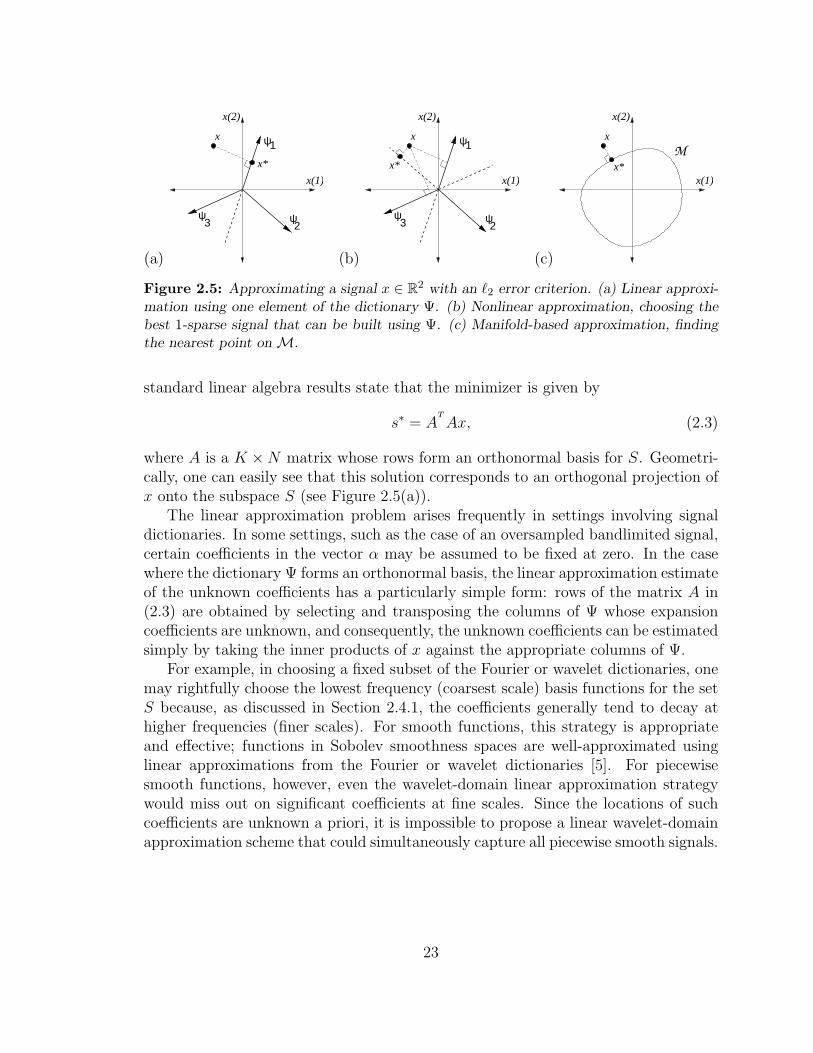
Figure 2.5: Approximating a signal x ∈ R2 with an `2 error criterion. (a) Linear approxi-mation using one element of the dictionary Ψ. (b) Nonlinear approximation, choosing thebest 1-sparse signal that can be built using Ψ. (c) Manifold-based approximation, findingthe nearest point onM.

standard linear algebra results state that the minimizer is given by

s∗ = AT

Ax, (2.3)

where A is a K ×N matrix whose rows form an orthonormal basis for S. Geometri-cally, one can easily see that this solution corresponds to an orthogonal projection ofx onto the subspace S (see Figure 2.5(a)).

The linear approximation problem arises frequently in settings involving signaldictionaries. In some settings, such as the case of an oversampled bandlimited signal,certain coefficients in the vector α may be assumed to be fixed at zero. In the casewhere the dictionary Ψ forms an orthonormal basis, the linear approximation estimateof the unknown coefficients has a particularly simple form: rows of the matrix A in(2.3) are obtained by selecting and transposing the columns of Ψ whose expansioncoefficients are unknown, and consequently, the unknown coefficients can be estimatedsimply by taking the inner products of x against the appropriate columns of Ψ.

For example, in choosing a fixed subset of the Fourier or wavelet dictionaries, onemay rightfully choose the lowest frequency (coarsest scale) basis functions for the setS because, as discussed in Section 2.4.1, the coefficients generally tend to decay athigher frequencies (finer scales). For smooth functions, this strategy is appropriateand effective; functions in Sobolev smoothness spaces are well-approximated usinglinear approximations from the Fourier or wavelet dictionaries [5]. For piecewisesmooth functions, however, even the wavelet-domain linear approximation strategywould miss out on significant coefficients at fine scales. Since the locations of suchcoefficients are unknown a priori, it is impossible to propose a linear wavelet-domainapproximation scheme that could simultaneously capture all piecewise smooth signals.

23

2.5.2 Nonlinear approximation

A related question often arises in settings involving signal dictionaries. Ratherthan finding the best approximation to a signal f using a fixed collection ofK elementsfrom the dictionary Ψ, one may often seek the best K-term representation to f amongall possible expansions that use K terms from the dictionary. Compared to linearapproximation, this type of nonlinear approximation [6, 7] utilizes the ability of thedictionary to adapt: different elements may be important for representing differentsignals.

The K-term nonlinear approximation problem corresponds to the optimization

s∗K,p := arg mins∈ΣK

‖s− f‖p. (2.4)

(For the sake of generality, we consider general Lp and `p norms in this section.) Dueto the nonlinearity of the set ΣK for a given dictionary, solving this problem can bedifficult. Supposing Ψ is an orthonormal basis and p = 2, the solution to (2.4) iseasily obtained by thresholding: compute the coefficients α and keep the K largest.The approximation error is then given simply by

‖s∗K,2 − f‖2 =

(∑

k>K

α2k

)1/2

.

When Ψ is a redundant dictionary, however, the situation is much more complicated.We mention more on this below (see also Figure 2.5(b)).

Measuring approximation quality

One common measure for the quality of a dictionary Ψ in approximating a signalclass is the fidelity of its K-term representations. Often one examines the asymptoticrate of decay of the K-term approximation error as K grows large. Defining

σK(f)p := ‖s∗K,p − f‖p, (2.5)

for a given signal f we may consider the asymptotic decay of σK(f)p as K →∞. (Werecall the dependence of (2.4) and hence (2.5) on the dictionary Ψ.) In many cases,the function σK(f)p will decay as K−r for some r, and when Ψ represents a harmonicdictionary, faster decay rates tend to correspond to smoother functions. Indeed, onecan show that when Ψ is an orthonormal basis, then σK(f)2 will decay as K−r if andonly if αk decays as k−r+1/2 [78].

Nonlinear approximation of piecewise smooth functions

Let f ∈ CH be a 1-D function. Supposing the wavelet dictionary has more than Hvanishing moments, then f can be well approximated using its K largest coefficients

24

(most of which are at coarse scales). As K grows large, the nonlinear approximationerror will decay4 as σK(f)2 . K−H .

Supposing that f is piecewise smooth, however, with a finite number of discon-tinuities, then (as discussed in Section 2.4.2) f will have a limited number of signif-icant wavelet coefficients at fine scales. Because of the concentration of these sig-nificant coefficients within each scale, the nonlinear approximation rate will remainσK(f)2 . K−H as if there were no discontinuities present [5].

Unfortunately, this resilience of wavelets to discontinuities does not extend tohigher dimensions. Suppose, for example, that f is a CH smooth 2-D signal. Assumingthe proper number of vanishing moments, a wavelet representation will achieve theoptimal nonlinear approximation rate σK(f)2 . K−H/2 [5,79]. As in the 1-D case, thisapproximation rate is maintained when a finite number of point discontinuities areintroduced into f . However, when f contains 1-D discontinuities (edges separatingthe smooth regions), the approximation rate will fall to σK(f)2 . K−1/2 [5]. Theproblem actually arises due to the isotropic, dyadic supports of the wavelets; insteadof O(1) significant wavelets at each scale, there are now O(2j) wavelets overlappingthe discontinuity. We revisit this important issue in Section 2.6.

Finding approximations

As mentioned above, in the case where Ψ is an orthonormal basis and p = 2, thesolution to (2.4) is easily obtained by thresholding: compute the coefficients α andkeep the K largest. Thresholding can also be shown to be optimal for arbitrary `pnorms in the special case where Ψ is the canonical basis. While the optimality ofthresholding does not generalize to arbitrary norms and bases, thresholding can beshown to be a near-optimal approximation strategy for wavelet bases with arbitraryLp norms [78].

In the case where Ψ is a redundant dictionary, however, the expansion coefficientsα are not unique, and the optimization problem (2.4) can be much more difficultto solve. Indeed, supposing even that an exact K-term representation exists for fin the dictionary Ψ, finding that K-term approximation is NP-complete in general,requiring a combinatorial enumeration of the

(ZK

)possible sparse subspaces [28]. This

search can be recast as the optimization problem

α = arg min ‖α‖0 s.t. f = Ψα. (2.6)

While solving (2.6) is prohibitively complex, a variety of algorithms have been pro-posed as alternatives. One approach convexifies the optimization problem by replac-ing the `0 fidelity criterion by an `1 criterion

α = arg min ‖α‖1 s.t. f = Ψα.

4We use the notation f(α) . g(α), or f(α) = O(g(α)), if there exists a constant C, possibly largebut not dependent on the argument α, such that f(α) ≤ Cg(α).

25

This problem, known as Basis Pursuit [80], is significantly more approachable andcan be solved with traditional linear programming techniques whose computationalcomplexities are polynomial in Z. Iterative greedy algorithms such as MatchingPursuit (MP) and Orthogonal Matching Pursuit (OMP) [5] have also been suggestedto find sparse representations α for a signal f . Both MP and OMP iteratively selectthe columns from Ψ that are most correlated with f , then subtract the contributionof each column, leaving a residual. OMP includes an additional step at each iterationwhere the residual is orthogonalized against the previously selected columns.

2.5.3 Manifold approximation

We also consider the problem of finding the best manifold-based approximationto a signal (see Figure 2.5(c)). Suppose that F = fθ : θ ∈ Θ is a parametrized K-dimension manifold and that we are given a signal I that is believed to approximatefθ for an unknown θ ∈ Θ. From I we wish to recover an estimate of θ. Again, wemay formulate this parameter estimation problem as an optimization, writing theobjective function (here we concentrate solely on the L2 or `2 case)

D(θ) = ‖fθ − I‖22and solving for

θ∗ = arg minθ∈Θ

D(θ).

We suppose that the minimum is uniquely defined.Standard nonlinear parameter estimation [81] tells us that, ifD is differentiable, we

can use Newton’s method to iteratively refine a sequence of guesses θ(0), θ(1), θ(2), . . .to θ∗ and rapidly convergence to the true value. Supposing that F is a differentiablemanifold, we would let

J = [∂D/∂θ0 ∂D/∂θ1 . . . ∂D/∂θK−1]T

be the gradient of D, and let H be the K ×K Hessian, Hij = ∂2D∂θi∂θj

. Assuming D is

differentiable, Newton’s method specifies the following update step:

θ(k+1) ← θ(k) + [H(θ(k))]−1J(θ(k)).

To relate this method to the structure of the manifold, we can actually express thegradient and Hessian in terms of signals, writing

D(θ) = ‖fθ − I‖22 =

∫(fθ − I)2 dx =

∫f 2

θ − 2Ifθ + I2 dx.

26

Differentiating with respect to component θi, we obtain

∂D

∂θi

= Ji =∂

∂θi

(∫f 2

θ − 2Ifθ + I2 dx

)

=

∫∂

∂θi

(f 2θ )− 2I

∂

∂θi

fθ dx

=

∫2fθτ

iθ − 2Iτ i

θ dx

= 2〈fθ − I, τ iθ〉,

where τ iθ = ∂fθ

∂θiis a tangent signal. Continuing, we examine the Hessian,

∂2D

∂θi∂θj

= Hij =∂

∂θj

(∂D

∂θi

)

=

∫∂

∂θj

(2fθτ

iθ − 2Iτ i

θ

)dx

=

∫2τ i

θτjθ + 2fθτ

ijθ − 2Iτ ij

θ dx

= 2〈τ iθ, τ

jθ 〉+ 2〈fθ − I, τ ij

θ 〉, (2.7)

where τ ijθ = ∂2fθ

∂θi∂θjdenotes a second-derivative signal. Thus, we can interpret New-

ton’s method geometrically as (essentially) a sequence of successive projections ontotangent spaces on the manifold.

Again, the above discussion assumes the manifold to be differentiable. However,as we discuss in Chapter 4, many interesting parametric signal manifolds are in factnowhere differentiable — the tangent spaces demanded by Newton’s method do notexist. However, we do identify a type of multiscale tangent structure to the manifoldthat permits a coarse-to-fine technique for parameter estimation. Section 4.5.2 detailsour Multiscale Newton method.

2.6 Compression

2.6.1 Transform coding

In Section 2.5.2, we measured the quality of a dictionary in terms of its K-termapproximations to signals drawn from some class. One reason that such approxima-tions are desirable is that they provide concise descriptions of the signal that can beeasily stored, processed, etc. There is even speculation and evidence that neurons inthe human visual system may use sparse coding to represent a scene [82].

For data compression, conciseness is often exploited in a popular technique knownas transform coding. Given a signal f (for which a concise description may not bereadily apparent in its native domain), the idea is simply to use the dictionary Ψ to

27

transform f to its coefficients α, which can then be efficiently and easily described.As discussed above, perhaps the simplest strategy for summarizing a sparse α issimply to threshold, keeping the K largest coefficients and discarding the rest. Asimple encoder would then just encode the positions and quantized values of these Kcoefficients.

2.6.2 Metric entropy

Suppose f is a function and let fR be an approximation to f encoded using R bits.To evaluate the quality of a coding strategy, it is common to consider the asymptoticrate-distortion (R-D) performance, which measures the decay rate of ‖f − fR‖Lp asR→∞. The metric entropy [57] for a class F gives the best decay rate that can beachieved uniformly over all functions f ∈ F . We note that this is a true measure forthe complexity of a class and is tied to no particular dictionary or encoding strategy.The metric entropy also has a very geometric interpretation, as it relates to thesmallest radius possible for a covering of 2R balls over the set F .

Metric entropies are known for certain signal classes. For example, the results ofClements [58] (extending those of Kolmogorov and Tihomirov [57]) regarding metricentropy give bounds on the optimal achievable asymptotic rate-distortion performancefor D-dimensional CH-smooth functions f (see also [79]):

∥∥∥f − fR

∥∥∥Lp

.

(1

R

)HD

.

Rate-distortion performance measures the complexity of a representation and en-coding strategy. In the case of transform coding, for example, R-D results accountfor the bits required to encode both the values of the significant coefficients and theirlocations. Nonetheless, in many cases transform coding is indeed an effective strat-egy for encoding signals that have sparse representations [7]. For example, in [79]Cohen et al. propose a wavelet-domain coder that uses a connected-tree structureto efficiently encode the positions of the significant coefficients and prove that thisencoding strategy achieves the optimal rate

∥∥∥f − fR

∥∥∥Lp

.

(1

R

)HD

.

2.6.3 Compression of piecewise smooth images

In some cases, however, the sparsity of the wavelet transform may not reflect thetrue underlying structure of a signal. Examples are 2-D piecewise smooth signalswith a smooth edge discontinuity separating the smooth regions. As we discussedin Section 2.5.2, wavelets fail to sparsely represent these functions, and so the R-Dperformance for simple thresholding-based coders will suffer as well. In spite of all

28

of the benefits of wavelet representations for signal processing (low computationalcomplexity, tree structure, sparse approximations for smooth signals), this failure toefficiently represent edges is a significant drawback. In many images, edges carrysome of the most prominent and important information [83], and so it is desirable tohave a representation well-suited to compressing edges in images.

To address this concern, recent work in harmonic analysis has focused on devel-oping representations that provide sparse decompositions for certain geometric imageclasses. Examples include curvelets [13, 14] and contourlets [73], slightly redundanttight frames consisting of anisotropic, “needle-like” atoms. In [84], bandelets areformed by warping an orthonormal wavelet basis to conform to the geometrical struc-ture in the image. A nonlinear multiscale transform that adapts to discontinuities(and can represent a “clean” edge using very few coarse scale coefficients) is proposedin [85]. Each of these new representations has been shown to achieve near-optimalasymptotic approximation and R-D performance for piecewise smooth images consist-ing of CH regions separated by discontinuities along CH curves, with H = 2 (H ≥ 2for bandelets). Some have also found use in specialized compression applications suchas identification photos [86].

In Chapter 3, we propose an alternative approach for representing and compress-ing piecewise smooth images in the wavelet domain, demonstrating that the lack ofwavelet sparsity can be overcome by using joint tree-based models for wavelet coef-ficients. Our scheme is based on the simple yet powerful observation that geometricfeatures can be efficiently approximated using local, geometric atoms in the spatialdomain, and that the projection of these geometric primitives onto wavelet subspacescan therefore approximate the corresponding wavelet coefficients. We prove that theresulting dictionary achieves the optimal nonlinear approximation rates for piecewisesmooth signal classes. To account for the added complexity of this encoding strategy,we also consider R-D results and prove that this scheme comes within a logarith-mic factor of the optimal performance rate. Unlike the techniques mentioned above,our method also generalizes to arbitrary orders of smoothness and arbitrary signaldimension.

2.7 Dimensionality Reduction

Recent years have seen a proliferation of novel techniques for what can loosely betermed “dimensionality reduction.” Like the tasks of approximation and compressiondiscussed above, these methods involve some aspect in which low-dimensional infor-mation is extracted about a signal or collection of signals in some high-dimensionalambient space. Unlike the tasks of approximation and compression, however, the goalof these methods is not always to maintain a faithful representation of each signal.Instead, the purpose may be to preserve some critical relationships among elementsof a data set or to discover information about a manifold on which the data lives.

In this section, we review two general methods for dimensionality reduction. Sec-

29

tion 2.7.1 begins with a brief overview of techniques for manifold learning. Sec-tion 2.7.2 then discusses the Johnson-Lindenstrauss (JL) lemma, which concerns theisometric embedding of a cloud points as it is projected to a lower-dimensional space.Though at first glance the JL lemma does not pertain to any of the low-dimensionalsignal models we have previously discussed, we later see (Section 2.8.6) that the JLlemma plays a critical role in the core theory of CS, and we also employ the JL lemmain developing a theory for isometric embeddings of manifolds (Theorem 6.2).

2.7.1 Manifold learning

Several techniques have been proposed for manifold learning in which a set ofpoints sampled from a K-dimensional submanifold of RN are mapped to some lowerdimension RM (ideally, M = K) while preserving some characteristic property ofthe manifold. Examples include ISOMAP [44], Hessian Eigenmaps (HLLE) [45], andMaximum Variance Unfolding (MVU) [46], which attempt to learn isometric embed-dings of the manifold (preserving pairwise geodesic distances); Locally Linear Em-bedding (LLE) [47], which attempts to preserve local linear neighborhood structuresamong the embedded points; Local Tangent Space Alignment (LTSA) [48], which at-tempts to preserve local coordinates in each tangent space; and a method for chartinga manifold [49] that attempts to preserve local neighborhood structures. These algo-rithms can be useful for learning the dimension and parametrizations of manifolds, forsorting data, for visualization and navigation through the data, and as preprocessingto make further analysis more tractable; common demonstrations include analysis offace images and classification of and handwritten digits. A related technique, theWhitney Reduction Network [41, 42], seeks a linear mapping to RM that preservesambient pairwise distances on the manifold and is particularly useful for processingthe output of dynamical systems having low-dimensional attractors.

Other algorithms have been proposed for characterizing manifolds from sampleddata without constructing an explicit embedding in RM . The Geodesic Minimal Span-ning Tree (GMST) [50] models the data as random samples from the manifold andestimates the corresponding entropy and dimensionality. Another technique [51] hasbeen proposed for using random samples of a manifold to estimate its homology (viathe Betti numbers, which essentially characterize its dimension, number of connectedcomponents, etc.). Persistence Barcodes [52] are a related technique that involvesconstructing a type of signature for a manifold (or simply a shape) that uses tangentcomplexes to detect and characterize local edges and corners.

Additional algorithms have been proposed for constructing meaningful functionson the point samples in RN . To solve a semi-supervised learning problem, a methodcalled Laplacian Eigenmaps [53] has been proposed that involves forming an adjacencygraph for the data in RN , computing eigenfunctions of the Laplacian operator on thegraph (which form a basis for L2 on the graph), and using these functions to train aclassifier on the data. The resulting classifiers have been used for handwritten digitrecognition, document classification, and phoneme classification. (The M smoothest

30

eigenfunctions can also be used to embed the manifold inM , similar to the approachesdescribed above.) A related method called Diffusion Wavelets [54] uses powers ofthe diffusion operator to model scale on the manifold, then constructs wavelets tocapture local behavior at each scale. The result is a wavelet transform adapted notto geodesic distance but to diffusion distance, which measures (roughly) the numberof paths connecting two points.

2.7.2 The Johnson-Lindenstrauss lemma

As with the above techniques in manifold learning, the Johnson-Lindenstrauss(JL) lemma [87–90] provides a method for dimensionality reduction of a set of datain RN . Unlike manifold-based methods, however, the JL lemma can be used for anyarbitrary set Q of points in RN ; the data set is not assumed to have any a prioristructure.

Despite the apparent lack of structure, the JL lemma suggests that the data setQ does carry information that can be preserved when the data is mapped to a lower-dimensional space RM . In particular, the original formulation of the JL lemma [87]states that there exists a Lipschitz mapping Φ : RN 7→ RM with M = O(log(#Q))such that all pairwise distances between points in Q are approximately preserved.This fact is useful for solving problems such as Approximate Nearest Neighbor [90], inwhich one desires the nearest point in Q to some query point y ∈ RN (but a solutionnot much further than the optimal point is also acceptable). Such problems can besolved significantly more quickly in RM than in RN .

Recent reformulations of the JL lemma propose random linear operators that,with high probability, will ensure a near isometric embedding. These typically buildon concentration of measure results such as the following.

Lemma 2.4 [88, 89] Let x ∈ RN , fix 0 < ε < 1, and let Φ be a matrix constructedin one of the following two manners:

1. Φ is a random M ×N matrix with i.i.d. N (0, σ2) entries, where σ2 = 1/N , or

2. Φ is random orthoprojector from RN to RM .

Then with probability exceeding

1− 2 exp

(−M(ε2/2− ε3/3)

2

),

the following holds:

(1− ε)√M

N≤ ‖Φx‖2‖x‖2

≤ (1 + ε)

√M

N. (2.8)

31

The random orthoprojector referred to above is clearly related to the first case(simple matrix multiplication by a Gaussian Φ) but subtly different; one could thinkof constructing a random Gaussian Φ, then using Gram-Schmidt to orthonormalizethe rows before multiplying x. (This adjustment could even be made after computingΦx, a fact which is possibly more relevant for results such as Theorem 6.2.) We note

also that simple rescaling of Φ can be used to eliminate the√

MN

in (2.8); however we

prefer this formulation for later reference.By using the union bound over all

(#Q2

)pairs of distinct points in Q, Lemma 2.4

can be used to prove a randomized version of the Johnson-Lindenstrauss lemma.

Lemma 2.5 (Johnson-Lindenstrauss) Let Q be a finite collection of points in RN .Fix 0 < ε < 1 and β > 0. Set

M ≥(

4 + 2β

ε2/2− ε3/3

)ln(#Q).

Let Φ be a matrix constructed in one of the following two manners:

1. Φ is a random M ×N matrix with i.i.d. N (0, σ2) entries, where σ2 = 1/N , or

2. Φ is random orthoprojector from RN to RM .

Then with probability exceeding 1− (#Q)−β, the following statement holds: for everyx, y ∈ Q,

(1− ε)√M

N≤ ‖Φx− Φy‖2‖x− y‖2

≤ (1 + ε)

√M

N.

Indeed, [88] establishes that both Lemma 2.4 and Lemma 2.5 also hold when theelements of Φ are chosen i.i.d. from a random Rademacher distribution (±σ with equalprobability 1/2) or from a similar ternary distribution (±

√3σ with equal probability

1/6; 0 with probability 2/3). These can further improve the computational benefitsof the JL lemma.

2.8 Compressed Sensing

A new theory known as Compressed Sensing (CS) has recently emerged that canalso be categorized as a type of dimensionality reduction. Like manifold learning,CS is strongly model-based (relying on sparsity in particular). However, unlike manyof the standard techniques in dimensionality reduction (such as manifold learning orthe JL lemma), the goal of CS is to maintain a low-dimensional representation of asignal x from which a faithful approximation to x can be recovered. In a sense, thismore closely resembles the traditional problem of data compression (see Section 2.6).In CS, however, the encoder requires no a priori knowledge of the signal structure.

32

Only the decoder uses the model (sparsity) to recover the signal. In Chapter 6, wewill indeed see that without changing the CS encoder we can also recover manifold-modeled signals simply by changing the decoder. We justify such an approach againusing geometric arguments.

2.8.1 Motivation

Consider a signal x ∈ RN , and suppose that the basis Ψ provides a K-sparserepresentation of x

x = Ψα,

with ‖α‖0 = K. (In this section, we focus on exactly K-sparse signals, though manyof the key ideas translate to compressible signals [20, 21]. In addition, we note thatthe CS concepts are also extendable to tight frames.)

As we discussed in Section 2.6, the standard procedure for compressing sparsesignals, known as transform coding, is to (i) acquire the full N -sample signal x;(ii) compute the complete set of transform coefficients α; (iii) locate the K largest,significant coefficients and discard the (many) small coefficients; (iv) encode the valuesand locations of the largest coefficients.

This procedure has three inherent inefficiencies: First, for a high-dimensionalsignal, we must start with a large number of samples N . Second, the encoder mustcompute all N of the transform coefficients α, even though it will discard all but Kof them. Third, the encoder must encode the locations of the large coefficients, whichrequires increasing the coding rate since the locations change with each signal.

2.8.2 Incoherent projections

This raises a simple question: For a given signal, is it possible to directly estimatethe set of large α(n)’s that will not be discarded? While this seems improbable,Candes, Romberg, and Tao [20, 22] and Donoho [21] have shown that a reducedset of projections can contain enough information to reconstruct sparse signals. Anoffshoot of this work, often referred to as Compressed Sensing (CS) [20,21,24–27,29],has emerged that builds on this principle.

In CS, we do not measure or encode the K significant α(n) directly. Rather, wemeasure and encode M < N projections y(m) = 〈x, φm

T 〉 of the signal onto a secondset of functions φm,m = 1, 2, . . . ,M . In matrix notation, we measure

y = Φx,

where y is an M × 1 column vector and the measurement basis matrix Φ is M × Nwith each row a basis vector φm. Since M < N , recovery of the signal x from themeasurements y is ill-posed in general; however the additional assumption of signalsparsity makes recovery possible and practical.

33

The CS theory tells us that when certain conditions hold, namely that the func-tions φm cannot sparsely represent the elements of the basis ψn (a conditionknown as incoherence of the two dictionaries [20–22,91]) and the number of measure-ments M is large enough, then it is indeed possible to recover the set of large α(n)(and thus the signal x) from a similarly sized set of measurements y. This incoherenceproperty holds for many pairs of bases, including for example, delta spikes and thesine waves of a Fourier basis, or the Fourier basis and wavelets. Significantly, thisincoherence also holds with high probability between an arbitrary fixed basis and arandomly generated one.

2.8.3 Methods for signal recovery

Although the problem of recovering x from y is ill-posed in general (becausex ∈ RN , y ∈ RM , and M < N), it is indeed possible to recover sparse signalsfrom CS measurements. Given the measurements y = Φx, there exist an infinitenumber of candidate signals in the shifted nullspace N (Φ) + x that could generatethe same measurements y (see Section 2.4.1). Recovery of the correct signal x can beaccomplished by seeking a sparse solution among these candidates.

Recovery via `0 optimization

Supposing that x is exactly K-sparse in the dictionary Ψ, then recovery of x fromy can be formulated as the `0 minimization

α = arg min ‖α‖0 s.t. y = ΦΨα. (2.9)

Given some technical conditions on Φ and Ψ (see Theorem 2.1 below), then with highprobability this optimization problem returns the proper K-sparse solution α, fromwhich the true x may be constructed. (Thanks to the incoherence between the twobases, if the original signal is sparse in the α coefficients, then no other set of sparsesignal coefficients α′ can yield the same projections y.) We note that the recoveryprogram (2.9) can be interpreted as finding a K-term approximation to y from thecolumns of the dictionary ΦΨ, which we call the holographic basis because of thecomplex pattern in which it encodes the sparse signal coefficients [21].

In principle, remarkably few incoherent measurements are required to recovera K-sparse signal via `0 minimization. Clearly, more than K measurements mustbe taken to avoid ambiguity; the following theorem establishes that K + 1 randommeasurements will suffice. (Similar results were established by Venkataramani andBresler [92].)

Theorem 2.1 Let Ψ be an orthonormal basis for RN , and let 1 ≤ K < N . Then thefollowing statements hold:

34

1. Let Φ be an M × N measurement matrix with i.i.d. Gaussian entries withM ≥ 2K. Then with probability one the following statement holds: all sig-nals x = Ψα having expansion coefficients α ∈ RN that satisfy ‖α‖0 = K canbe recovered uniquely from the M-dimensional measurement vector y = Φx viathe `0 optimization (2.9).

2. Let x = Ψα such that ‖α‖0 = K. Let Φ be an M ×N measurement matrix withi.i.d. Gaussian entries (notably, independent of x) with M ≥ K + 1. Then withprobability one the following statement holds: x can be recovered uniquely fromthe M-dimensional measurement vector y = Φx via the `0 optimization (2.9).

3. Let Φ be an M × N measurement matrix, where M ≤ K. Then, aside frompathological cases (specified in the proof), no signal x = Ψα with ‖α‖0 = K canbe uniquely recovered from the M-dimensional measurement vector y = Φx.

Proof: See Appendix A.

The second statement of the theorem differs from the first in the following respect:when K < M < 2K, there will necessarily exist K-sparse signals x that cannot beuniquely recovered from the M -dimensional measurement vector y = Φx. However,these signals form a set of measure zero within the set of all K-sparse signals and cansafely be avoided if Φ is randomly generated independently of x.

Unfortunately, as discussed in Section 2.5.2, solving this `0 optimization prob-lem is prohibitively complex. Yet another challenge is robustness; in the setting ofTheorem 2.1, the recovery may be very poorly conditioned. In fact, both of theseconsiderations (computational complexity and robustness) can be addressed, but atthe expense of slightly more measurements.

Recovery via `1 optimization

The practical revelation that supports the new CS theory is that it is not necessaryto solve the `0-minimization problem to recover α. In fact, a much easier problemyields an equivalent solution (thanks again to the incoherency of the bases); we needonly solve for the `1-sparsest coefficients α that agree with the measurements y [20–22,24–27,29]

α = arg min ‖α‖1 s.t. y = ΦΨα. (2.10)

As discussed in Section 2.5.2, this optimization problem, also known as Basis Pur-suit [80], is significantly more approachable and can be solved with traditional linearprogramming techniques whose computational complexities are polynomial in N .

There is no free lunch, however; according to the theory, more than K + 1 mea-surements are required in order to recover sparse signals via Basis Pursuit. Instead,one typically requires M ≥ cK measurements, where c > 1 is an oversampling factor.As an example, we quote a result asymptotic in N . For simplicity, we assume that

35

the sparsity scales linearly with N ; that is, K = SN , where we call S the sparsityrate.

Theorem 2.2 [28, 38, 39] Set K = SN with 0 < S 1. Then there exists anoversampling factor c(S) = O(log(1/S)), c(S) > 1, such that, for a K-sparse signalx in the basis Ψ, the following statements hold:

1. The probability of recovering x via Basis Pursuit from (c(S) + ε)K randomprojections, ε > 0, converges to one as N →∞.

2. The probability of recovering x via Basis Pursuit from (c(S) − ε)K randomprojections, ε > 0, converges to zero as N →∞.

In an illuminating series of recent papers, Donoho and Tanner [38–40] have char-acterized the oversampling factor c(S) precisely (see also Section 2.8.5). With ap-propriate oversampling, reconstruction via Basis Pursuit is also provably robust tomeasurement noise and quantization error [22].

In the remainder of this section and in Chapter 5, we often use the abbreviatednotation c to describe the oversampling factor required in various settings even thoughc(S) depends on the sparsity K and signal length N .

Recovery via greedy pursuit

At the expense of slightly more measurements, iterative greedy algorithms suchas Orthogonal Matching Pursuit (OMP) [91], Matching Pursuit (MP) [5], and TreeMatching Pursuit (TMP) [93, 94] have also been proposed to recover the signal xfrom the measurements y (see Section 2.5.2). In CS applications, OMP requiresc ≈ 2 ln(N) [91] to succeed with high probability. OMP is also guaranteed to convergewithin M iterations. In Chapter 5, we will exploit both Basis Pursuit and greedyalgorithms for recovering jointly sparse signals from incoherent measurements. Wenote that Tropp and Gilbert require the OMP algorithm to succeed in the first Kiterations [91]; however, in our simulations, we allow the algorithm to run up to themaximum of M possible iterations. While this introduces a potential vulnerability tonoise in the measurements, our focus in Chapter 5 is on the noiseless case. The choiceof an appropriate practical stopping criterion (likely somewhere between K and Miterations) is a subject of current research in the CS community.

2.8.4 Impact and applications

CS appears to be promising for a number of applications in signal acquisition andcompression. Instead of sampling a K-sparse signal N times, only cK incoherentmeasurements suffice, where K can be orders of magnitude less than N . Therefore,a sensor can transmit far fewer measurements to a receiver, which can reconstructthe signal and then process it in any manner. Moreover, the cK measurements need

36

not be manipulated in any way before being transmitted, except possibly for somequantization. Finally, independent and identically distributed (i.i.d.) Gaussian orBernoulli/Rademacher (random ±1) vectors provide a useful universal basis that isincoherent with all others. Hence, when using a random basis, CS is universal in thesense that the sensor can apply the same measurement mechanism no matter whatbasis the signal is sparse in (and thus the coding algorithm is independent of thesparsity-inducing basis) [20,21,95].

These features of CS make it particularly intriguing for applications in remotesensing environments that might involve low-cost battery operated wireless sensors,which have limited computational and communication capabilities. Indeed, in manysuch environments one may be interested in sensing a collection of signals using anetwork of low-cost signals. In Chapter 5, we propose a series of models for jointsparsity structure among a collection of signals, and we propose the correspondingalgorithms for Distributed Compressed Sensing (DCS) of such signals.

Other possible application areas of CS include imaging [33], medical imaging [22,96], and RF environments (where high-bandwidth signals may contain low-dimensionalstructures such as radar chirps) [97]. As research continues into practical methods forsignal recovery (see Section 2.8.3), additional work has focused on developing physicaldevices for acquiring random projections. Our group has developed, for example, aprototype digital CS camera based on a digital micromirror design [33]. Additionalwork suggests that standard components such as filters (with randomized impulseresponses) could be useful in CS hardware devices [98].

2.8.5 The geometry of Compressed Sensing

It is important to note that the core theory of CS draws from a number of deepgeometric arguments. For example, when viewed together, the CS encoding/decodingprocess can be interpreted as a linear projection Φ : RN 7→ RM followed by a non-linear mapping ∆ : RM 7→ RN . In a very general sense, one may naturally ask fora given class of signals F ∈ RN (such as the set of K-sparse signals or the set ofsignals with coefficients ‖α‖`p ≤ 1), what encoder/decoder pair Φ,∆ will ensure thebest reconstruction (minimax distortion) of all signals in F . This best-case perfor-mance is proportional to what is known as the Gluskin n-width [99,100] of F (in oursetting n = M), which in turn has a geometric interpretation. Roughly speaking, theGluskin n-width seeks the (N − n)-dimensional slice through F that yields signals ofgreatest energy. This n-width bounds the best-case performance of CS on classes ofcompressible signals, and one of the hallmarks of CS is that, given a sufficient numberof measurements this optimal performance is achieved (to within a constant) [21,78].

Additionally, one may view the `0/`1 equivalence problem geometrically. In par-ticular, given the measurements y = Φx, we have an (N−M)-dimensional hyperplaneHy = x′ ∈ RN : y = Φx′ = N (Φ) + x of feasible signals that could account for themeasurements y. Supposing the original signal x is K-sparse, the `1 recovery programwill recover the correct solution x if and only if ‖x′‖1 > ‖x‖1 for every other signal

37

x′ ∈ Hy on the hyperplane. This happens only if the hyperplane Hy (which passesthrough x) does not “cut into” the `1-ball of radius ‖x‖1. This `1-ball is a polytope,on which x belongs to a (K − 1)-dimensional “face.” If Φ is a random matrix withi.i.d. Gaussian entries, then the hyperplane Hy will have random orientation. To an-swer the question of how M must relate to K in order to ensure reliable recovery, ithelps to observe that a randomly generated hyperplane H will have greater chance toslice into the `1 ball as dim(H) = N−M grows (or as M shrinks) or as the dimensionK − 1 of the face on which x lives grows. Such geometric arguments have been madeprecise by Donoho and Tanner [38–40] and used to establish a series of sharp boundson CS recovery.

In Section 6.1.3, we will also present an alternative proof for the first statement inTheorem 2.1 based purely on geometric arguments (following, in fact, from a resultabout manifold embeddings).

2.8.6 Connections with dimensionality reduction

We have also identified [95] a fundamental connection between the CS and theJL lemma. In order to make this connection, we considered the Restricted IsometryProperty (RIP), which has been identified as a key property of the CS projectionoperator Φ to ensure stable signal recovery. We say Φ has RIP of order K if for everyK-sparse signal x,

(1− ε)√M

N≤ ‖Φx‖2‖x‖2

≤ (1 + ε)

√M

N.

A random M × N matrix with i.i.d. Gaussian entries can be shown to have thisproperty with high probability if M = O(K log(N/K)).

While the JL lemma concerns pairwise distances within a finite cloud of points,the RIP concerns isometric embedding of an infinite number of points (comprising aunion of K-dimensional subspaces in RN). However, the RIP can in fact be derivedby constructing an effective sampling of K-sparse signals in RN , using the JL lemmato ensure isometric embeddings for each of these points, and then arguing that theRIP must hold true for all K-sparse signals. (See [95] for the full details.)

In Chapter 6, we will again employ the JL lemma to prove that manifolds also havenear-isometric embeddings under random projections to lower-dimensional space; thisfact will allow us to extend the applicability of CS beyond sparse signal recovery toinclude parameter estimation and manifold learning from random measurements.

38

Chapter 3Parametric Representation and Compression of

Multi-Dimensional Piecewise Functions

In this chapter1 we consider the task of approximating and compressing two modelclasses of functions for which traditional harmonic dictionaries fail to provide sparserepresentations. However, the model itself dictates a low-dimensional structure to thesignals, which we capture using a novel parametric multiscale dictionary.

The functions we consider are both highly relevant in signal processing and highlystructured. In particular, we consider piecewise constant signals in P dimensionswhere a smooth (P −1)-dimensional discontinuity separates the two constant regions,and we also consider the extension of this class to piecewise smooth signals, wherea smooth (P − 1)-dimensional discontinuity separates two smooth regions. Thesesignal classes provide basic models, for example, for images containing edges, videosequences of moving objects, or seismic data containing geological horizons.

Despite the underlying (indeed, low-dimensional) structure in each of these classes,classical harmonic dictionaries fail to provide sparse representations for such signals.The problem comes from the (P − 1)-dimensional discontinuity, whose smooth geo-metric structure is not captured by local isotropic representations such as wavelets.

As a remedy, we propose a multiscale dictionary consisting of local parametricatoms called surflets, each a piecewise constant function with a (tunable) polynomialdiscontinuity separating the two constant regions. Our surflet dictionary falls outsidethe traditional realm of bases and frames (where approximations are assembled as lin-ear combinations of atoms from the dictionary). Rather, our scheme is perhaps betterviewed as a “geometric tiling,” where precisely one atom from the dictionary is usedto describe the signal at each part of the domain (these atoms “tile” together to coverthe domain). We discuss multiscale, tree-based schemes for assembling and encodingsurflet representations, and we prove that such schemes attain optimal asymptotic ap-proximation and compression performance on our piecewise constant function classes.

We also see limitations to this scheme, however. As designed for piecewise con-stant functions, our surflet model fails to account for relevant activity away from thediscontinuity. Turning our attention, then, to the problem of approximating and com-pressing piecewise smooth functions, we propose a hybrid scheme combining surflets

1This work is in collaboration with Venkat Chandrasekaran, Dror Baron, and Richard Bara-niuk [101] and also builds upon earlier work in collaboration with Justin Romberg, Hyeokho Choi,and Richard Baraniuk [102].

39

with wavelets. Our scheme is based on the simple yet powerful observation that geo-metric features can be efficiently approximated using local surflet atoms in the spatialdomain, and that the projection of these geometric primitives onto wavelet subspacescan therefore approximate the corresponding wavelet coefficients — we dub the result-ing projections surfprints. Hence we develop an entirely wavelet-domain approxima-tion and compression scheme for piecewise smooth signals, where wavelet coefficientsnear edges are grouped together (as surfprints) and described parametrically. Weprove that surfprint/wavelet schemes attain near-optimal asymptotic approximationand compression performance on our piecewise smooth function classes.

Our work in this chapter can be viewed as a generalization of the wedgelet [103]and wedgeprint [102] representations. (Wedgelets are 2-D atoms localized on dyadicsquares with a straight edge separating two constant regions.) Our extensions in thischapter, however, provide fundamental new insights in the following directions:

• The wedgelet and wedgeprint dictionaries are restricted to 2-D signals, whileour proposed representations are relevant in higher dimensions.

• Wedgelets and wedgeprints achieve optimal approximation rates only for func-tions that are C2-smooth and contain a C2-smooth discontinuity; our results notonly show that surflets and surfprints can be used to achieve optimal rates formore general classes, but also highlight the necessary polynomial orders andquantization scheme (a nontrivial extension from wedgelets).

• We also present a more thorough analysis of discretization effects, includingnew insights on the multiscale behavior (not revealed by considering wedgeletsalone), a new strategy for reducing the surflet dictionary size at fine scales, andthe first treatment of wedgeprint/surfprint discretization.

This chapter is organized as follows. In Section 3.1, we define our function mod-els and state the specific goals of our approximation and compression algorithms.We introduce surflets in Section 3.2. In Section 3.3, we describe our surflet-basedrepresentation schemes for piecewise constant functions. In Section 3.4, we presentour novel dictionary of wavelets and surfprints for effectively representing piecewisesmooth functions. Section 3.5 discusses extensions to discrete data and presents nu-merical experiments.

3.1 Function Classes and Performance Bounds

3.1.1 Multi-dimensional signal models

In this chapter, we consider functions over the continuous domain [0, 1]P . We letx = [x1, x2, · · · , xP ] ∈ [0, 1]P denote an arbitrary point in this domain. (Note theuse boldface characters to denote vectors in this chapter.) We denote the first P − 1elements of x by y, i.e., y = [x1, x2, · · · , xP−1] ∈ [0, 1]P−1.

40

(a)x

x

1

2

f([ , ])x2x1

b( )x1

x

x

1

2

b([ , ])x2x1

x3

f([ , , ])x2x1 x3

(b)x

x

1

2

Figure 3.1: (a) Piecewise constant (“Horizon-class”) functions for dimensions P = 2 andP = 3. (b) Piecewise smooth function for dimension P = 2.

We will often find it useful construct a P -dimensional function by combining twoP -dimensional functions separated by a (P − 1)-dimensional discontinuity. As anexample, suppose that g1 and g2 are functions of P variables

g1, g2 : [0, 1]P → R,

and that b is a function of P − 1 variables

b : [0, 1]P−1 → R.

We define the function f : [0, 1]P → R in the following piecewise manner:

f(x) =

g1(x), xP ≥ b(y)g2(x), xP < b(y).

Piecewise constant model

The first class of functions we consider is a “piecewise constant” case where g1 = 1and g2 = 0. In this case, the (P − 1)-dimensional discontinuity b defines a boundarybetween two constant regions in P dimensions. (Piecewise constant functions f de-fined in this manner are sometimes known as Horizon-class functions [103].) Whenb ∈ CHd , with Hd = rd+νd, we denote the resulting space of functions f by FC(P,Hd).When P = 2, these functions can be interpreted as images containing a CHd-smoothone-dimensional discontinuity that separates a 0-valued region below from a 1-valuedregion above. For P = 3, functions in FC(P,Hd) can be interpreted as cubes witha 2-D CHd-smooth surface cutting through them, dividing them into two regions —0-valued below the surface and 1-valued above it (see Figure 3.1(a) for examples in2-D and 3-D).

We often use f c to denote an arbitrary function in FC(P,Hd), in such cases wedenote its (P − 1)-dimensional CHd-smooth discontinuity by bc.

41

Piecewise smooth model

The second class of functions we consider is a “piecewise smooth” model. Forthis class of functions, we let g1, g2 ∈ CHs , with Hs = rs + νs, and b ∈ Hd, withHd = rd + νd. The resulting piecewise smooth function f consists of a (P − 1)-dimensional CHd-smooth discontinuity that separates two CHs-smooth regions in Pdimensions (see Figure 3.1(b) for an example in 2-D). We denote the class of suchpiecewise smooth functions by FS(P,Hd, Hs). One can check that both FC(P,Hd)and the space of P -dimensional uniformly CHs functions are subsets of FS(P,Hd, Hs).

We often use f s to denote an arbitrary function in FS(P,Hd, Hs). For such afunction, we denote the (P − 1)-dimensional CHd-smooth discontinuity by bs and theP -dimensional CHs-smooth regions by gs

1 and gs2.

3.1.2 Optimal approximation and compression rates

In this chapter, we define dictionaries of atoms from which we construct an approx-imation f to f , which may belong to FC(P,Hd) or FS(P,Hd, Hs). We analyze the per-formance of our coding scheme using the squared-L2 distortion measure between theP -dimensional functions f and f . We measure the ability of our dictionary of atomsto represent f sparsely by the asymptotic approximation performance ‖f − fN‖2L2

as

N →∞, where fN is the best N -term approximant to f . We also present compressionalgorithms that encode those atoms from the corresponding dictionaries (depending

on whether f ∈ FC(P,Hd) or f ∈ FS(P,Hd, Hs)) used to construct f . We measurethe performance of these compression algorithms by the asymptotic rate-distortionfunction ‖f − fR‖2L2

R → ∞, where fR is the best approximation to f that can beencoded using R bits [104].

A function belonging to either class FC(P,Hd) or FS(P,Hd, Hs) contains a certaindegree of structure due to the smooth functions of which it is comprised. (One of thesecomponent functions is not only smooth but has lower dimension than f .) Indeed,we see that the optimal approximation and compression performance rates derivedirectly from these degrees of smoothness.

In [79], Cohen et al. establish the optimal approximation rate for D-dimensionalCH-smooth functions d: ∥∥∥d− dN

∥∥∥2

Lp

.

(1

N

) 2HD

.

Similarly, as we discussed in Section 2.6, the optimal achievable asymptotic rate-distortion performance for D-dimensional CH-smooth functions d is given by

∥∥∥d− dR

∥∥∥2

Lp

.

(1

R

) 2HD

.

These results, however, are only useful for characterizing optimal separate representa-tions for the (P−1)-dimensional discontinuity and the P -dimensional smooth regions.

42

We extend these results to non-separable representations of the P -dimensionalfunction classes FC(P,Hd) and FS(P,Hd, Hs) in Theorems 3.1 and 3.2, respectively.

Theorem 3.1 The optimal asymptotic approximation performance that can be ob-tained for all f c ∈ FC(P,Hd) is given by

∥∥∥f c − f cN

∥∥∥2

L2

.

(1

N

) HdP−1

.

Similarly, the optimal asymptotic compression performance that can be obtained forall f c ∈ FC(P,Hd) is given by

∥∥∥f c − f cR

∥∥∥2

L2

.

(1

R

) HdP−1

.

Proof: See [101, Appendix A].

Implicit in the proof of the above theorem is that any scheme that is optimalfor representing and compressing the P -dimensional function f c ∈ FC(P,Hd) in thesquared-L2 sense is equivalently optimal for the (P − 1)-dimensional discontinuity inthe L1 sense. Roughly, the squared-L2 distance between two Horizon-class functionsf c

1 and f c2 over a P -dimensional domain D = [D1

b,D1e ]× · · · × [DP

b ,DPe ] is equal to the

L1 distance over the (P − 1)-dimensional subdomain [D1b,D1

e ] × · · · × [DP−1b ,DP−1

e ]between the (P − 1)-dimensional discontinuities bc1 and bc2 in f c

1 and f c2 respectively.

More precisely and for future reference, for every y in the (P − 1)-dimensionalsubdomain of D, we define the D-clipping of a (P − 1)-dimensional function b as

b(y) =

b(y), DPb ≤ b(y) ≤ DP

e

DPe , b(y) > DP

e

DPb , b(y) < DP

b .

The D-active region of b is defined to be

y ∈ [D1

b,D1e ]× · · · × [DP−1

b ,DP−1e ] : b(y) ∈ [DP

b ,DPe ],

that subset of the subdomain of D for which the range of b lies in [DPb ,DP

e ]. TheD-clipped L1 distance between bc1 and bc2 is then defined as

L1(bc1, b

c2) =

∥∥bc1 − bc2∥∥

L1([D1b,D1

e ]×···×[DP−1b ,DP−1

e ]).

One can check that ‖f c1 − f c

2‖2L2(D) = L1(bc1, b

c2) for any D.

The following theorem characterizes the optimal achievable asymptotic approxi-mation rate and rate-distortion performance for approximating and encoding elementsof the function class FS(P,Hd, Hs).

43

Theorem 3.2 The optimal asymptotic approximation performance that can be ob-tained for all f s ∈ FS(P,Hd, Hs) is given by

∥∥∥f s − f sN

∥∥∥2

L2

.

(1

N

)min(

HdP−1

, 2HsP

)

.

Similarly, the optimal asymptotic compression performance that can be obtained forall f s ∈ FS(P,Hd, Hs) is given by

∥∥∥f s − f sR

∥∥∥2

L2

.

(1

R

)min(

HdP−1

, 2HsP

)

.

Proof: See [101, Appendix B].

3.1.3 “Oracle” coders and their limitations

In order to approximate or compress an arbitrary function f c ∈ FC(P,Hd), wepresume that an algorithm is given the function f c itself. Again, however, all ofthe critical information about f c is contained in the discontinuity bc, and one wouldexpect any efficient coder to exploit such a fact. Methods through which this isachieved may vary.

One can imagine a coder that explicitly encodes an approximation bc to bc andthen constructs a Horizon approximation f c. Knowledge of bc could be provided froman external “oracle” [105], or bc could conceivably be estimated from the provideddata f c. As discussed in Section 2.6.2, a tree-structured wavelet coder could provideone efficient method for compressing the (P −1)-dimensional smooth function bc withoptimal L1 rate-distortion performance. Such a wavelet/Horizon coder would thenbe optimal (in the squared-L2 sense) for coding instances of f c at the optimal rate ofTheorem 3.1. In practice, however, a coder would not provided with explicit infor-mation of bc, and a method for estimating bc from f c may be difficult to implement.Estimates for bc may also be quite sensitive to noise in the data.

A similar strategy could also be employed for f s ∈ FS(P,Hd, Hs). Approximations

to the discontinuity bs and the P -dimensional smooth regions gs1 and gs

2 may beencoded separately and explicitly. This strategy would have disadvantages for thesame reasons mentioned above. In fact, estimating the discontinuity in this scenariowould be much harder.

In this chapter, we seek and propose representation schemes and algorithms thatapproximate f c and f s directly in P dimensions. For our surflet and surfprint schemes,we emphasize that no explicit knowledge of the functions bc, bs, gs

1, or gs2 is required.

We prove that surflet-based approximation techniques and encoding algorithms forf c achieve the optimal decay rates, while our surfprint-based methods for f s achievethe optimal approximation decay rate and a near-optimal rate-distortion decay rate(within a logarithmic factor of the optimal decay rate of Theorem 3.2). Although

44

we omit the discussion, our algorithms can be extended to similar piecewise constantand piecewise smooth function spaces. Our spatially localized approach, for exam-ple, allows for changes in the variable along which the discontinuity varies (assumedthroughout this chapter to be xP as described in Section 3.1.1).

3.2 The Surflet Dictionary

In this section, we introduce a discrete, multiscale dictionary of P -dimensionalatoms called surflets that can be used to construct approximations to a functionf c ∈ FC(P,Hd). A surflet is a piecewise constant function defined on a P -dimensionaldyadic hypercube, where a (P−1)-dimensional polynomial specifies the discontinuity.Section 3.3 describes compression using surflets.

3.2.1 Motivation — Taylor’s theorem

The surflet atoms are motivated by the following property. If d is a function of Dvariables in CH with H = r + ν, r is a positive integer, and ν ∈ (0, 1], then Taylor’stheorem states that

d(z + h) = d(z) +1

1!

D∑

i1=1

dzi1(z)hi1 +

1

2!

D∑

i1,i2=1

dzi1,zi2

(z)hi1hi2 + · · ·

+1

r!

D∑

i1,...,ir=1

dzi1,··· ,zir

(z)hi1 · · ·hir +O(‖h‖H), (3.1)

where dz1,··· ,z`refers to the iterated partial derivatives of d with respect to z1, . . . , z` in

that order. (Note that there are D` `’th order derivative terms.) Thus, over a smalldomain, the function d is well approximated using a polynomial of order r (where thepolynomial coefficients correspond to the partial derivatives of d evaluated at z).

Clearly, in the case of f c, one method for approximating the discontinuity bc

would be to assemble a piecewise polynomial approximation, where each polynomialis derived from the local Taylor approximation of bc (let D = P − 1, H = Hd, andd = bc in the above characterization). These piecewise polynomials can be used toassemble a Horizon-class approximation of the function f c. Surflets provide the P -dimensional framework for constructing such approximations and can be implementedwithout explicit knowledge of bc or its derivatives.

45

3.2.2 Definition

Recall from Section 2.1.5 that a dyadic hypercube Xj ⊆ [0, 1]P at scale j ∈ N is adomain that satisfies2

Xj = [β12−j, (β1 + 1)2−j)× · · · × [βP 2−j, (βP + 1)2−j)

with β1, β2, . . . , βP ∈ 0, 1, . . . , 2j − 1. We explicitly denote the (P − 1)-dimensionalhypercube subdomain of Xj as

Yj = [β12−j, (β1 + 1)2−j)× · · · × [βP−12

−j, (βP−1 + 1)2−j). (3.2)

The surflet s(Xj; p; ·) is a Horizon-class function over the dyadic hypercubeXj definedthrough the (P − 1)-dimensional polynomial p. For x ∈ Xj with correspondingy = [x1, x2, · · · , xP−1],

s(Xj; p;x) =

1, xP ≥ p(y)0, otherwise,

where the polynomial p(y) is defined as

p(y) = p0 +P−1∑

i1=1

p1,i1 yi1 +P−1∑

i1,i2=1

p2,i1,i2 yi1yi2 + · · ·+P−1∑

i1,...,ird=1

prd,i1,i2,...,irdyi1yi2 · · · yird

.

We call the polynomial coefficients p`,i1,...,i`rd`=0 the surflet coefficients.3 We note

here that, in some cases, a surflet may be identically 0 or 1 over the entire domainXj. We sometimes denote a generic surflet by s(Xj), indicating only its region ofsupport.

A surflet s(Xj) approximates the function f c over the dyadic hypercube Xj. Onecan cover the entire domain [0, 1]P with a collection of dyadic hypercubes (possiblyat different scales) and use surflets to approximate f c over each of these smallerdomains. For P = 3, these surflets tiled together look like piecewise polynomial“surfaces” approximating the discontinuity bc in the function f c. Figure 3.2 illustratesa collection of surflets with P = 2 and P = 3.

2In this chapter we use half-open intervals, but in order to cover the entire domain [0, 1]P , in thecase where (βi + 1)2−j = 1, i ∈ 1, . . . , P, we replace the half-open interval [βi2

−j , (βi + 1)2−j)with the closed interval [βi2

−j , (βi + 1)2−j ].3Because the ordering of the terms yi1yi2 · · · yi`

in a monomial is irrelevant, only(`+P−2

`

)mono-

mial coefficients (not (P − 1)`) need to be encoded for order `. We preserve the slightly redundantnotation for ease of comparison with (3.1).

46

(a) (b) (c) (d)

Figure 3.2: Example surflets, designed for (a) P = 2, Hd ∈ (1, 2]; (b) P = 2, Hd ∈ (2, 3];(c) P = 3, Hd ∈ (1, 2]; (d) P = 3, Hd ∈ (2, 3].

3.2.3 Quantization

We obtain a discrete surflet dictionary S(j) at scale j by quantizing the set ofallowable surflet polynomial coefficients. For ` ∈ 0, 1, . . . , rd, the surflet coefficientp`,i1,...,i` at scale j ∈ N is restricted to values µ ·∆Hd

`,j µ∈Z, where the stepsize satisfies

∆Hd`,j = 2−(Hd−`)j. (3.3)

The necessary range for µ will depend on the derivative bound Ω (Section 2.1.4). Weemphasize that the relevant discrete surflet dictionary S(j) is finite at every scale j.

These quantization stepsizes are carefully chosen to ensure the proper fidelity ofsurflet approximations without requiring excess bitrate. The key idea is that higher-order terms can be quantized with lesser precision without increasing the residualerror term in the Taylor approximation (3.1). In fact, Kolmogorov and Tihomirov [57]implicitly used this concept to establish the metric entropy for bounded uniformlysmooth functions.

3.3 Approximation and Compression of Piecewise ConstantFunctions

3.3.1 Overview

We now propose a surflet-based multiresolution geometric tiling approach to ap-proximate and encode an arbitrary function f c ∈ FC(P,Hd). The tiling is arrangedon a 2P -tree, where each node in the tree at scale j corresponds to a hypercube ofsidelength 2−j. Each node is labeled with a surflet appropriately chosen from S(j)and is either a leaf node (hypercube) or has 2P children nodes (children hypercubesthat perfectly tile the volume of the parent hypercube). Leaf nodes provide the ac-tual approximation to the function f c, while interior nodes are useful for predictingand encoding their descendants. This framework enables an adaptive, multiscale ap-proximation of f c — many small surflets can be used at fine scales for complicatedregions, while few large surflets will suffice to encode simple regions of f c (such asthose containing all 0 or 1). Figure 3.3 shows surflet tiling approximations for P = 2and P = 3.

47

(a) (b)

Figure 3.3: Example surflet tilings, (a) piecewise cubic with P = 2 and (b) piecewiselinear with P = 3.

Section 3.3.2 discusses techniques for determining the proper surflet at each node.Section 3.3.3 describes a constructive algorithm for building tree-based surflet approx-imations. Section 3.3.4 describes the performance of a simple surflet encoder actingonly on the leaf nodes. Section 3.3.5 presents a more advanced surflet coder, usinga top-down predictive technique to exploit the correlation among surflet coefficients.Finally, Section 3.3.6 discusses extensions of our surflet-based representation schemesto broader function classes.

3.3.2 Surflet selection

Consider a node at scale j that corresponds to a dyadic hypercube Xj, and let Yj

be the (P − 1)-dimensional subdomain of Xj as defined in (3.2).We first examine a situation where the coder is provided with explicit information

about the discontinuity bc and its derivatives. In this case, determination of the surfletat the node that corresponds to Xj can proceed as implied by Section 3.2. The coderconstructs the Taylor expansion of bc around any point y ∈ Yj and quantizes thepolynomial coefficients (3.3). We choose

yep =

[(β1 +

1

2

)2−j,

(β2 +

1

2

)2−j, . . . ,

(βP−1 +

1

2

)2−j

]

and call this an expansion point. We refer to the resulting surflet as the quantizedTaylor surflet. From (3.1), it follows that the squared-L2 error between f c and thequantized Taylor surflet approximation s(Xj) (which equals the Xj-clipped L1 errorbetween bc and the polynomial defining s(Xj)) obeys

‖f c − s(Xj)‖2L2(Xj)=

∫

Xj

(f c − s(Xj))2 = O

(2−j(Hd+P−1)

). (3.4)

However, as discussed in Section 3.1.3, our coder is not provided with explicit in-formation about bc. Therefore, approximating functions in FC(P,Hd) using Taylor

48

surflets is impractical.4

We now define a technique for obtaining a surflet estimate directly from the func-tion f c. We assume that there exists a method to compute the squared-L2 error‖f c − s(Xj)‖2L2(Xj)

between a given surflet s(Xj) and the function f c on the dyadic

block Xj. In such a case, we can search the finite surflet dictionary S(j) for theminimizer of this error without explicit knowledge of bc. We refer to the resultingsurflet as the native L2-best surflet; this surflet will necessarily obey (3.4) as well.Practically speaking, there may be certain challenges to solving this L2 optimizationproblem. These challenges are revealed by taking a geometric perspective, viewing theparameter estimation problem as the orthogonal projection from f c onto the manifoldof possible surflets. As we discuss in Chapter 4, this manifold is not differentiable,which poses an apparent barrier to techniques that might invoke the manifold’s tan-gent spaces in order to apply calculus-based optimization. However, in Chapter 4, wealso introduce a multiscale estimation algorithm designed to circumvent this difficulty.

Section 3.3.4 discusses the coding implications of using L2-best surflets from S(j).Using native L2-best surflets over dyadic blocks Xj achieves near-optimal perfor-mance. As will be made apparent in Section 3.3.5, in order to achieve optimal perfor-mance, a coder must exploit correlations among nearby surflets. Unfortunately, thesecorrelations may be difficult to exploit using native L2-best surflets. The problemarises because surflets with small Xj-active regions (Section 3.1.2) may be close in L2

distance over Xj yet have vastly different underlying polynomial coefficients. (Thesecoefficients are used explicitly in our encoding strategy.)

To resolve this problem, we suggest computing L2-best surflet fits to f c over theL-extension of each dyadic hypercube Xj. That is, if Xj = [β12

−j, (β1 + 1)2−j) ×· · · × [βP 2−j, (βP + 1)2−j) then the L-extension of Xj is defined to be

XLj = [(β1 − L)2−j, (β1 + 1 + L)2−j)× · · · × [(βP − L)2−j, (βP + 1 + L)2−j),

where L > 0 is an extension factor (designed to expand the domain of analysis andincrease correlations between scales).5 An L-extended surflet is a surflet from S(j)that is now defined over XL

j whose polynomial discontinuity has a non-empty Xj-active region. We define the L-extended surflet dictionary SL(j) to be the set ofL-extended surflets from S(j) plus the all-zero and all-one surflets s(Xj) = 0 ands(Xj) = 1. An L-extended L2-best surflet fit to f c over Xj is then defined to be theL2-best surflet to f c over XL

j chosen from SL(j). Note that even though extendedsurflets are defined over extended domains XL

j , they are used to approximate thefunction only over the associated native domains Xj. Such extended surflet fits (overextended domains) provide sufficient mathematical constraints for a coder to relatenearby surflets, since extended surflets that are close in terms of squared-L2 distance

4We refer the reader to a technical report [106] for a thorough treatment of Taylor surflet-basedapproximation of piecewise constant multi-dimensional functions.

5If necessary, each L-extension is truncated to the hypercube [0, 1]P .

49

over XLj have similar polynomial coefficients (even if extended surflets have small

Xj-active regions, they have large XLj -active regions). In Section 3.3.5, we describe a

coder that uses extended surflets from SL(j) to achieve optimal performance.

3.3.3 Tree-based surflet approximations

The surflet dictionary consists of P -dimensional atoms at various scales. Thus, a2P -tree offers a natural topology for arranging the surflets used in an approximation.Specifically, each node at scale j in a 2P -tree is labeled by a surflet that approximatesthe corresponding dyadic hypercube region Xj of the function f c. This surflet can beassigned according to any of the procedures outlined in Section 3.3.2.

Given a method for assigning a surflet to each tree node, it is also necessary todetermine the proper dyadic segmentation for the tree approximation. This can beaccomplished using the CART algorithm, which is based on dynamic programming,in a process known as tree-pruning [103,107]. Tree-pruning proceeds from the bottomup, determining whether to prune the tree beneath each node (causing it to becomea leaf node). Various criteria exist for making such a decision. In particular, theapproximation-theoretic optimal segmentation can be obtained by minimizing the La-grangian cost D+λN for a penalty term λ. Similarly, the Lagrangian rate-distortioncost D + λR can be used to obtain the optimal rate-distortion segmentation.

We summarize the construction of a surflet-based approximation as follows:

Surflet-based approximation

• Choose scale: Choose a maximal scale J ∈ Z for the 2P -tree.

• Label all nodes: For each scale j = 0, 1, . . . , J , label all nodes at scale j witheither a native or an extended L2-best surflet chosen appropriately from eitherdiscrete dictionary of surflets S(j) or SL(j).

• Prune tree: Starting at the second-finest scale j = J − 1, determine whethereach node at scale j should be pruned (according to an appropriate pruningrule). Then proceed up to the root of the tree, i.e., until j = 0.

The approximation performance of this algorithm is described in the following theo-rem.

Theorem 3.3 Using either quantized Taylor surflets or L2-best surflets (extended ornative), a surflet tree-pruned approximation of an element f c ∈ FC(P,Hd) achievesthe optimal asymptotic approximation rate of Theorem 3.1:

∥∥∥f c − f cN

∥∥∥2

L2

.

(1

N

) HdP−1

.

Proof: See [101, Appendix C].

50

3.3.4 Leaf encoding

An initial approach toward surflet encoding would involve specification of thetree segmentation map (which denotes the location of the leaf nodes) along with thequantized surflet coefficients at each leaf node. Rate-distortion analysis then yieldsthe following result.

Theorem 3.4 Using either quantized Taylor surflets or L2-best surflets (extendedor native), a surflet leaf-encoder applied to an element f c ∈ FC(P,Hd) achieves thefollowing rate-distortion performance

∥∥∥f c − f cR

∥∥∥2

L2

.

(logR

R

) HdP−1

.

Proof: See [101, Appendix D].

Comparing with Theorem 3.1, this simple coder is near-optimal in terms of rate-distortion performance. The logarithmic factor is due to the fact that it requires O(j)bits to encode each surflet at scale j. In Section 3.3.5, we propose an alternative coderthat requires only a constant number of bits to encode each surflet.

3.3.5 Top-down predictive encoding

Achieving the optimal performance of Theorem 3.1 requires a more sophisticatedcoder that can exploit the correlation among nearby surflets. We now briefly describea top-down surflet coder that predicts surflet parameters from previously encodedvalues.

Top-down predictive surflet coder

• Encode root node: Encode the best surflet fit s([0, 1]P ) to the hypercube[0, 1]P . Encode a flag (1-bit) specifying whether this node is interior or a leaf.Set j ← 0.

• Predict surflets from parent scale: For every interior node/hypercube Xj

at scale j, partition its domain into 2P children hypercubes at scale j + 1.Compute the polynomial coefficients on each child hypercube Xj+1 that agreewith the encoded parent surflet s(XL

j ). These serve as “predictions” for thepolynomial coefficients at the child.

• Encode innovations at child nodes: For each predicted polynomial coeffi-cient, encode the discrepancy with the L-extended surflet fit s(XL

j+1).

• Descend tree: Set j ← j + 1 and repeat until no interior nodes remain.

51

This top-down predictive coder encodes an entire tree segmentation starting with theroot node, and proceeding from the top down. Given an L-extended surflet s(XL

j ) atan interior node at scale j, we show in [101, Appendix E] that the number of possibleL-extended surflets from SL(j) that can be used for approximation at scale j + 1 isconstant, independent of the scale j. Thus, given a best-fit surflet at scale 0, a constantnumber of bits is required to encode each surflet at subsequent scales. This predictionis possible because L-extended surflets are defined over L-extended domains, whichensures coherency between the surflet fits (and polynomial coefficients) at a parentand child node.

We note that predicting L-extended best-fit surflets to dyadic hypercube regionsaround the borders of [0, 1]P may not be possible with a constant number of bits whenthe discontinuity is not completely contained within the dyadic hypercube. However,we make the mild simplifying assumption that the intersections of the discontinuitywith the hyperplanes xP = 0 or xP = 1 can be contained within O(2(P−2)j) hyper-cubes at each scale j. Therefore, using O(Hdj) bits to encode such “border” dyadichypercubes (with the discontinuity intersecting xP = 0 or xP = 1) does not affect theasymptotic rate-distortion performance of the top-down predictive coder.

Theorem 3.5 The top-down predictive coder applied to an element f c ∈ FC(P,Hd)using L-extended L2-best surflets from SL(j) achieves the optimal rate-distortion per-formance of Theorem 3.1:

∥∥∥f c − f cR

∥∥∥2

L2

.

(1

R

) HdP−1

.

Proof: See [101, Appendix E].

Although only the leaf nodes provide the ultimate approximation to the function,the additional information encoded at interior nodes provides the key to efficientlyencoding the leaf nodes. In addition, unlike the surflet leaf-encoder of Section 3.3.3,this top-down approach yields a progressive bitstream — the early bits encode alow-resolution (coarse scale) approximation, which is then refined using subsequentbits.

3.3.6 Extensions to broader function classes

Our results for classes of functions that contain a single discontinuity can be ex-tended to spaces of signals that contain multiple discontinuities. Functions containingmultiple discontinuities that do not intersect can be represented using the surflet-based approximation scheme described in Section 3.3.3 at the optimal asymptoticapproximation rate. This is because at a sufficiently high scale, dyadic hypercubesthat tile signals containing multiple non-intersecting discontinuities contain at mostone discontinuity.

52

Analysis of the surflet-based approximation scheme of Section 3.3.3 applied tosignals containing intersecting discontinuities is more involved. Let f c

] be a P -dimensional piecewise constant function containing two (P − 1)-dimensional CHd-smooth discontinuities that intersect each other (the analysis that follows can easilybe extended to allow for more than two intersecting discontinuities). Note that theintersection of (P − 1)-dimensional functions forms a (P − 2)-dimensional manifold.Again, we make the mild simplifying assumption that the intersection of the disconti-nuities can be contained in O(2(P−2)j) hypercubes at each scale j. The following theo-rem describes the approximation performance achieved by the scheme in Section 3.3.3applied to f c

] . A consequence of this theorem is that there exists a smoothness thresh-

old Hthd that defines the boundary between optimal and sub-optimal approximation

performance.

Theorem 3.6 Using either quantized Taylor surflets or L2-best surflets (extendedor native), the approximation scheme of Section 3.3.3 applied to a piecewise con-stant P -dimensional function f c

] that contains two intersecting CHd-smooth (P − 1)-dimensional discontinuities achieves performance given by:

• P > 2, Hd ≤ 2(P−1)P−2

:

∥∥∥f c] − f c

],N

∥∥∥2

L2

.

(1

N

) HdP−1

.

• P > 2, Hd >2(P−1)

P−2:

∥∥∥f c] − f c

],N

∥∥∥2

L2

.

(1

N

) 2P−2

.

• P = 2, any Hd:∥∥∥f c

] − f c],N

∥∥∥2

L2

.

(1

N

) HdP−1

.

Proof: See [101, Appendix F].

Thus, the representation scheme in Section 3.3.3 achieves optimal approximationperformance for P = 2 even in the presence of intersecting discontinuities, while itachieves optimal performance for P > 2 up to a smoothness threshold of Hth

d = 2(P−1)P−2

(for Hd > Hthd , the scheme performs sub-optimally: ‖f c

] − f c],N‖2L2

.(

1N

) Hthd

P−1 ).This performance of the approximation scheme for P > 2 is still superior to thatof wavelets, which have Hth,wl

d = 1. The reason for this difference in performancebetween the cases P = 2 and P > 2 is that intersections of discontinuities when

53

P = 2 correspond to points,6 while intersections in higher dimensions correspondto low-dimensional manifolds. Hence, the number of hypercubes that contain inter-sections in the two-dimensional case is constant with scale, whereas the number ofhypercubes that contain the intersections when P > 2 grows exponentially with scale.The analysis above can clearly be extended to prove analogous results for functionscontaining piecewise CHd-smooth discontinuities.

Future work will focus on improving the threshold Hthd for the case P > 2. In

order to achieve optimal performance for P > 2, one may need a dictionary contain-ing regular surflets and specially-designed “intersection” surflets that are specificallytailored for intersections.

3.4 Approximation and Compression of Piecewise SmoothFunctions

In this section, we extend our coding strategies for piecewise constant functionsto encoding an arbitrary element f s from the class FS(P,Hd, Hs) of piecewise smoothfunctions.

3.4.1 Motivation

For a CHs-smooth function f in P dimensions, a wavelet basis with sufficient van-ishing moments provides approximations at the optimal rate [79] — ‖f − fN‖2L2

.(

1N

) 2HsP (see also Section 2.5.2). Even if one introduces a finite number of point sin-

gularities into the P -dimensional CHs-smooth function, wavelet-based approximationschemes still attain the optimal rate. Wavelets succeed in approximating smoothfunctions because most of the wavelet coefficients have small magnitudes and canthus be neglected. Moreover, an arrangement of wavelet coefficients on the nodes of atree leads to an interesting consequence: wavelet coefficients used in the approxima-tion of P -dimensional smooth functions are coherent — often, if a wavelet coefficienthas small magnitude, then its children coefficients also have small magnitude. Theseproperties of the wavelet basis have been exploited in state-of-the-art wavelet-basedimage coders [9, 11].

Although wavelets approximate smooth functions well, the wavelet basis is notwell-equipped to approximate functions containing higher-dimensional manifold dis-continuities. As discussed in Section 2.5.2, wavelets also do not take advantage ofany structure (such as smoothness) that the (P − 1)-dimensional discontinuity mighthave, and therefore many high-magnitude coefficients are often required to representdiscontinuities. Regardless of the smoothness order of the discontinuity, the approxi-mation rate achieved by wavelets remains the same.

6Our analysis also applies to “T-junctions” in images, where one edge terminates at its intersectionwith another.

54

Figure 3.4: Example surflet and the corresponding surfprint. The white box is the dyadichypercube in which we define the surflet; note that the removal of coarse scale and neigh-boring wavelets causes the surfprint to appear different from the surflet.

Despite this drawback, we desire a wavelet domain solution to approximate f s ∈FS(P,Hd, Hs) because most of the function f s is smooth in P dimensions, exceptfor a (P − 1)-dimensional discontinuity. In order to solve the problem posed by thediscontinuity, we propose the addition of surfprint atoms to the dictionary of waveletatoms. A surfprint is a weighted sum of wavelet basis functions derived from theprojection of a piecewise polynomial surflet atom (a (P − 1)-dimensional polynomialdiscontinuity separating two P -dimensional polynomial regions) onto a subspace inthe wavelet domain (see Figure 3.4 for an example in 2-D). Surfprints possess allthe properties that make surflets well-suited to represent discontinuities. In addition,surfprints coherently model wavelet coefficients that correspond to discontinuities.Thus, we obtain a single unified wavelet-domain framework that is well-equipped tosparsely represent both discontinuities and smooth regions.

The rest of this section is devoted to the definition of surfprints and their use ina wavelet domain framework to represent and encode approximations to elements ofFS(P,Hd, Hs). We do not discuss the extension of our results to classes of piecewisesmooth signals containing multiple intersecting discontinuities, but note that such ananalysis would be similar to that described in Section 3.3.6.

3.4.2 Surfprints

Let XJo be a dyadic hypercube at scale Jo. Let v1, v2 be P -dimensional polyno-mials of degree rsp

s , and let v be a P -dimensional function as follows:

v1, v2, v : XJo → R.

Let q be a (P − 1)-dimensional polynomial of degree rspd :

q : YJo → R.

55

As defined in Section 3.1.1, let x ∈ XJo and let y denote the first P − 1 elements ofx. Let the P -dimensional piecewise polynomial function v be defined as follows:

v(x) =

v1(x), xP ≥ q(y)v2(x), xP < q(y).

Next, we describe how this piecewise polynomial function is projected onto a waveletsubspace to obtain a surfprint atom. Let W be a compactly supported wavelet basisin P dimensions with Hwl

s vanishing moments. A surfprint sp(v,XJo ,W) is a weightedsum of wavelet basis functions with the weights derived by projecting the piecewisepolynomial v onto the subtree of basis functions whose idealized supports nest in thehypercube XJo :

sp(v,XJo ,W) =∑

j≥Jo,Xj⊆XJo

⟨v, wXj

⟩wXj

, (3.5)

where wXjrepresents the wavelet basis function having idealized compact support on

the hypercube Xj. (The actual support of wXjmay extend slightly beyond Xj.) The

hypercube XJo thus defines the root node (or coarsest scale) of the surfprint atom.We propose an approximation scheme in Section 3.4.5 where we use wavelet atoms

to represent uniformly smooth regions of f s and surfprint atoms to represent regionsthrough which the discontinuity passes. Before presenting our approximation scheme,we begin in Section 3.4.3 by describing how to choose the surfprint polynomial degreesrsps and rsp

d and the number of vanishing moments Hwls for the wavelet basis.

3.4.3 Vanishing moments and polynomial degrees

In general, when approximating elements f s ∈ FS(P,Hd, Hs), the required surf-print polynomial degrees and wavelet vanishing moments are determined by the ordersof smoothness Hd and Hs:

Hwls ≥ Hs, rsp

d = dHd − 1e, and rsps = dHs − 1e.

(This is due to Taylor’s theorem.) However, the exponent in the expression of Theo-rem 3.2 for the optimal approximation rate for FS(P,Hd, Hs) indicates that for every(Hd, Hs), either the (P − 1)-dimensional discontinuity or the P -dimensional smoothregion dominates the decay rate. For instance, in two dimensions, the smaller of thetwo smoothness orders Hd and Hs defines the decay rate.7 This implies that the surf-print polynomial degrees and/or the number of wavelet vanishing moments can berelaxed (as if either the discontinuity or the smooth regions had a lower smoothnessorder), without affecting the approximation rate.

7We note also that in the case where the functions g1 and g2, which characterize f s aboveand below the discontinuity, have differing orders of smoothness, the smaller smoothness order willdetermine both the achievable approximation rates and the appropriate approximation strategies.

56

Rather than match the surfprint parameters directly to the smoothness ordersHd and Hs, we let Hsp

d and Hsps denote the operational smoothness orders to which

the surfprint parameters are matched. These operational smoothness orders are se-lected to ensure the best approximation or rate-distortion performance. The detailedderivations of [101, Appendices G–H] yield the following values for the operationalsmoothness orders:

• Discontinuity dominates: In this case, Hd

P−1< 2Hs

P. We let Hsp

d = Hd and

choose Hsps ∈ [Hd−1

2, Hs] and Hwl

s ∈ [ HdP2(P−1)

, Hs].

• Smooth regions dominate: In this case, 2Hs

P< Hd

P−1. We let Hwl

s = Hs, and

choose Hsps ∈ [Hs(1− 1

P)− 1

2, Hs] and Hsp

d ∈ [2Hs(P−1)P

, Hd].

• Both contribute equally: In this case, 2Hs

P= Hd

P−1. We let Hwl

s = Hs,

Hspd = Hd, and choose Hsp

s ∈ [Hs(1− 1P)− 1

2, Hs].

The surfprint polynomial degrees are given by

rspd = dHsp

d − 1e and rsps = dHsp

s − 1e.

Therefore, if dHspd − 1e < dHd − 1e and dHsp

s − 1e < dHs − 1e, then the requiredsurfprint polynomial degrees for optimal approximations are lower than what onewould naturally expect. Note that even in the scenario where both terms in theexponent of the approximation rate match, one can choose Hsp

s slightly smaller thanHs while still attaining the optimal approximation rate of Theorem 3.2.

3.4.4 Quantization

In order to construct a discrete surfprint/wavelet dictionary, we quantize the co-efficients of the wavelet and surfprint atoms. The quantization step-size ∆Hwl

s for thewavelet coefficients depends on the specific parameters of an approximation scheme.We present our prototype approximation scheme and discuss the wavelet coefficientstep-sizes in Section 3.4.5 (see (3.8) below).

The quantization step-size for the surfprint polynomial coefficients of order ` atscale j is analogous to the step-size used to construct a discrete surflet dictionary(3.3):

∆Hsp

d`,j = 2−(Hsp

d −`)j (3.6)

and∆Hsp

s`,j = 2−(Hsp

s −`)j. (3.7)

As before, the key idea is that higher-order polynomial coefficients can be quantizedwith lesser precision without affecting the error term in the Taylor approximation(3.1).

57

3.4.5 Surfprint-based approximation

We present a tree-based representation scheme using quantized wavelet and surf-print atoms and prove that this scheme achieves the optimal approximation rate forevery function f s ∈ FS(P,Hd, Hs). Let W be a compactly supported wavelet basisin P dimensions with Hwl

s vanishing moments, as defined in Section 3.4.3. Considerthe decomposition of f s into the wavelet basis vectors: f s =

∑j〈f s, wXj

〉wXj. The

wavelet coefficients 〈f s, wXj〉 are quantized according to the step-size ∆Hwl

s definedbelow. Let these wavelet atoms be arranged on the nodes of a 2P -tree. We classifythe nodes based on the idealized support of the corresponding wavelet basis functions.Nodes whose supports Xj are intersected by the discontinuity bs are called Type Dnodes. All other nodes (over which f s is smooth) are classified as Type S. Considernow the following surfprint approximation strategy:8

Surfprint approximation

• Choose scales and wavelet quantization step-size: Choose a maximalscale J ∈ Z and m,n ∈ Z such that m

n= P

P−1and both m and n divide J . The

quantization step-size for wavelet coefficients at all scales j is given by:

∆Hwls = 2−

Jm

(Hwls +P

2) (3.8)

and thus depends only on the maximal scale J and the parameter m.

• Prune tree: Keep all wavelet nodes up to scale Jm

; from scale Jm

to scale Jn,

prune the tree at all Type S nodes (discarding those wavelet coefficients andtheir descendant subtrees).

• Select surfprint atoms: At scale Jn

replace the wavelet atom at each Type Ddiscontinuity node and its descendant subtree (up to depth J) by a quantizedsurfprint atom chosen appropriately from the dictionary with Jo = J

nin (3.5):

– P -dimensional polynomials: Choose P -dimensional polynomials v1 andv2 of degree rsp

s = dHsps − 1e. These polynomials should approximate

the P -dimensional smooth regions up to an absolute (pointwise) error of

O(2

−Hsps Jn

). The existence of such polynomials is guaranteed by Taylor’s

theorem (3.1) (let D = P , H = Hsps , and r = rsp

s ) and the quantizationscheme (3.7).

– (P−1)-dimensional polynomial: Choose a (P−1)-dimensional polynomialq of degree rsp

d = dHspd − 1e such that the discontinuity is approximated up

8The wavelet decomposition actually has 2P − 1 distinct directional subbands; we assume herethat each is treated identically. Also we assume the scaling coefficient at the coarsest scale j = 0 isencoded as side information with negligible cost.

58

to an absolute error of O

(2

−Hspd

J

n

). The existence of such a polynomial

is guaranteed by Taylor’s theorem (3.1) (let D = P − 1, H = Hspd , and

r = rspd ) and the quantization scheme of (3.6).

The following theorem summarizes the performance analysis for such surfprint ap-proximations.

Theorem 3.7 A surfprint-based approximation of an element f s ∈ FS(P,Hd, Hs) aspresented above achieves the optimal asymptotic approximation rate of Theorem 3.2:

∥∥∥f s − f sN

∥∥∥2

L2

.

(1

N

)min(

HdP−1

, 2HsP

)

.

Proof: See [101, Appendix G].

An approximation scheme that uses the best configuration of N wavelet and surf-print atoms in the L2 sense would perform at least as well as the scheme suggestedabove. Hence, surfprint approximation algorithms designed to choose the best N -term approximation (even without explicit knowledge of the discontinuity or theP -dimensional smooth regions) will achieve the optimal approximation rate of Theo-rem 3.2.

3.4.6 Encoding a surfprint/wavelet approximation

We now consider the problem of encoding the tree-based approximation of Sec-tion 3.4.5. A simple top-down coding scheme that specifies the pruned tree topology,quantized wavelet coefficients, and surfprint parameters achieves a near-optimal rate-distortion performance.

Theorem 3.8 A coding scheme that encodes every element of the surfprint-basedapproximation of an element f s ∈ FS(P,Hd, Hs) as presented in Section 3.4.5 achievesthe near-optimal asymptotic rate-distortion performance (within a logarithmic factorof the optimal performance of Theorem 3.2):

∥∥∥f s − f sR

∥∥∥2

L2

.

(logR

R

)min(

HdP−1

, 2HsP

)

.

Proof: See [101, Appendix H].

Repeating the argument of Section 3.4.5, this near optimal rate-distortion perfor-mance serves as an upper bound for an encoding scheme that encodes elements of anL2-best approximation. We will discuss the extension of these theoretical results tothe approximation of discrete data and related issues in Section 3.5.3.

59

3.5 Extensions to Discrete Data

3.5.1 Overview

In this section, we consider the problem of representing discrete data obtained by“voxelizing” (or pixelizing in 2-D) functions from the classes FC(P,Hd) and FS(P,Hd, Hs).Let f be a continuous P -dimensional function. We discretize f according to a vectorπ = [2π1 , . . . , 2πP ] ∈ ZP , which specifies the number of voxels along each dimension of

the discretized P -dimensional function fπ. Each entry of fπ is obtained either by av-eraging f over a P -dimensional voxel or by sampling f at uniformly spaced intervals.(Because of the smoothness characteristics of FC(P,Hd) and FS(P,Hd, Hs), both dis-cretization mechanisms provide the same asymptotic performance.) In our analysis,we allow the number of voxels along each dimension to vary in order to provide aframework for analyzing various sampling rates along the different dimensions. Videodata, for example, is often sampled differently in the spatial and temporal dimensions.Future research will consider different distortion criteria based on asymmetry in thespatiotemporal response of the human visual system.

For our analysis, we assume that the voxelization vector π is fixed and denotethe resulting classes of voxelized functions by FC(P,Hd) and FS(P,Hd, Hs). Sec-

tions 3.5.2 and 3.5.3 describe the sparse representation of elements from FC(P,Hd)

and FS(P,Hd, Hs), respectively. In Section 3.5.4, we discuss the impact of discretiza-tion effects on fine scale approximations. Finally, we present our simulation resultsin Section 3.5.5.

3.5.2 Representing and encoding elements of FC(P,Hd)

Suppose f c ∈ FC(P,Hd) and let f cπ ∈ FC(P,Hd) be its discretization. (We

view f cπ as a function on the continuous domain [0, 1]P that is constant over each

voxel.) The process of voxelization affects the ability to approximate elements of

FC(P,Hd). At coarse scales, however, much of the intuition for coding FC(P,Hd)

can be retained. In particular, we can bound the distance from f cπ to f c. We

note that f cπ differs from f c only over voxels through which b passes. Because

each voxel has size 2−π1 × 2−π2 · · · × 2−πP , the number of voxels intersected by b is

O(2∑P−1

i=1 πi

⌈(Ω · 2−min(πi)

P−1i=1

)/ (2−πP )

⌉), where Ω is the universal derivative bound

(Section 2.1.4). The squared-L2 distortion incurred on each such voxel (assumingonly that the voxelization process is bounded and local) is O(2−(π1+···+πP )). Summingover all voxels it follows that the (nonsquared) L2 distance obeys

∥∥∥f c − f cπ

∥∥∥L2([0,1]P )

< C1 · 2−(min πi)/2 (3.9)

where the minimum is taken over all i ∈ 1, . . . , P.Now we consider the problem of encoding elements of FC(P,Hd). At a particular

60

bitrate R, we know from Theorem 3.1 that no encoder could represent all elements

of FC(P,Hd) using R bits and incurring L2 distortion less than C2 ·(

1R

) Hd2(P−1) . (This

lower bound for metric entropy is in effect for R sufficiently large, which we assume tobe the case.) Suppose we consider a hypothetical encoder for elements of FC(P,Hd)

that, using R bits, could represent any element with L2 distortion of FC(P,Hd) lessthan some Dhyp(R). This coder could also be used as an encoder for elements ofFC(P,Hd) (by voxelizing each function before encoding). This strategy would yieldL2 distortion no worse than C1 ·2−(min πi)/2+Dhyp(R). By applying the metric entropyarguments on FC(P,Hd), we have the following constraint on Dhyp(R):

C1 · 2−(min πi)/2 +Dhyp(R) ≥ C2 ·(

1

R

) Hd2(P−1)

,

or equivalently,

Dhyp(R) ≥ C2 ·(

1

R

) Hd2(P−1)

− C1 · 2−(min πi)/2. (3.10)

This inequality helps establish a rate-distortion bound for the class FC(P,Hd).

At sufficiently low rates, the first term on the RHS dominates, and FC(P,Hd) facessimilar rate-distortion constraints to FC(P,Hd). At high rates, however, the RHS

becomes negative, giving little insight into the coding of FC(P,Hd). This breakdownpoint occurs when R ∼ 2(min πi)(P−1)/Hd .

We can, in fact, specify a constructive encoding strategy for FC(P,Hd) thatachieves the optimal compression rate up to this breakdown point. We constructa dictionary of discrete surflet atoms by voxelizing the elements of the continuousquantized surflet dictionary. Assuming there exists a technique to find discrete `2-best surflet fits to f c

π, the tree-based algorithm described in Section 3.3.3 can simply

be used to construct an approximationf c

π.

Theorem 3.9 While R . 2(min πi)(P−1)/Hd, the top-down predictive surflet coder from

Section 3.3.5 applied to encode the approximationf c

π to f cπ using discrete `2-best sur-

flets achieves the rate-distortion performance

∥∥∥∥f cπ −

f c

π

∥∥∥∥2

L2

.

(1

R

) HdP−1

.

Proof: See [101, Appendix I].

As detailed in the proof of this theorem, the breakdown point occurs when usingsurflets at a critical scale Jvox = min πi

Hd. Up to this scale, all of the familiar approxi-

mation and compression rates hold. Beyond this scale, however, voxelization effects

61

dominate. An interesting corollary to Theorem 3.9 is that, due to the similarities up

to scale Jvox, the discrete approximationf c

π itself provides an effective approximationto the function f c.

Corollary 3.1 While R . 2(min πi)(P−1)/Hd, the discrete approximationf c

π providesan approximation to f c with the following rate-distortion performance:

∥∥∥∥f c − f cπ

∥∥∥∥2

L2

.

(1

R

) HdP−1

.

Proof: See [101, Appendix J].

While we have provided an effective strategy for encoding elements of FC(P,Hd)at sufficiently low rates (using surflets at scales j ≤ Jvox), this leaves open the question

of how to code FC(P,Hd) at higher rates. Unfortunately, (3.10) does not offer muchinsight. In particular, it is not clear whether surflets are an efficient strategy forencoding FC(P,Hd) beyond scale Jvox. We revisit this issue in Section 3.5.4.

3.5.3 Representing and encoding elements of FS(P,Hd, Hs)

Next, let f sπ be an arbitrary signal belonging to FS(P,Hd, Hs). Similar arguments

apply to the voxelization effects for this class. In order to approximate functionsin FS(P,Hd, Hs), we use a dictionary of compactly supported discrete wavelet basisfunctions with Hwl

s vanishing moments and discrete surfprint atoms. A discrete surf-print atom is derived by projecting a discrete piecewise polynomial surflet atom ontoa subspace of the discrete wavelet basis.

We use the scheme described in Section 3.4.5 with Jvox

n= min(πi)

min(Hspd ,2Hsp

s +1)to ap-

proximate f sπ by

f s

π. According to [101, Appendix H], this scale corresponds to a range

of bitrates up to O(Jvox2(P−1)Jvox

n ). Within this range, the approximation is encodedas described in Section 3.4.6. The performance of this scheme appears below.

Theorem 3.10 While R . Jvox2(P−1)Jvox

n where Jvox = n·min(πi)

min(Hspd ,2Hsp

s +1), the coding

scheme from Section 3.4.5 applied to encode the approximationf s

π to f sπ using a

discrete wavelet/surfprint dictionary achieves the following near-optimal asymptoticrate-distortion performance (within a logarithmic factor of the optimal performanceof Theorem 3.2):

∥∥∥∥f sπ −

f s

π

∥∥∥∥2

L2

.

(logR

R

)min(

HdP−1

, 2HsP

)

.

62

Proof: See [101, Appendix K].

Again, a corollary follows naturally.

Corollary 3.2 While R . Jvox2(P−1)Jvox

n , the discrete approximationf s

π provides anapproximation to f s with the following rate-distortion performance:

∥∥∥∥f s − f sπ

∥∥∥∥2

L2

.

(logR

R

)min(

HdP−1

, 2HsP

)

.

Proof: See [101, Appendix L].

3.5.4 Discretization effects and varying sampling rates

We have proposed surflet algorithms for discrete data at sufficiently coarse scales.Unfortunately, this leaves open the question of how to represent such data at finerscales. In this section, we discuss one perspective on fine scale approximation thatleads to a natural surflet coding strategy.

Consider again the class FC(P,Hd). Section 3.5.2 provided an effective strategy

for encoding elements of FC(P,Hd) at sufficiently low rates (using surflets at scalesj ≤ Jvox = min πi

Hd). Beyond scale Jvox, however, the voxelization effects dominate

the resolution afforded by surflet approximations. To restore a balance, we suggest acoding strategy for finer scales based on the observation that FC(P,Hd) ⊂ FC(P,H)forH < Hd. Surflet approximations on the class FC(P,H) (tied to the smoothnessH)

have lower accuracy in general. As a result, FC(P,H) has a higher “breakdown rate”

than FC(P,Hd), and discrete surflets tailored for smoothnessH will achieve the codingrate O(R−H/(P−1)) up to scale min πi

H. While this may not be a worthwhile strategy

before scale Jvox, it could be useful beyond scale Jvox and up to scale min πi

H. In fact,

beyond that scale, we can again reduce H, obtaining a new breakdown rate and a finerscale to code (using lower-order surflets). This gives us a concrete strategy for coding

FC(P,Hd) at all scales, although our optimality arguments apply only up to scale

Jvox. At scale j, we use surflets designed for smoothness Hj = min(Hd,

min(πi)j

), 0 ≤

j ≤ min(πi). A surflet dictionary constructed using such scale-adaptive smoothnessorders consists of relatively few elements at coarse scales (due to the low value of jin the quantization stepsize) and relatively few at fine scales (due to the decrease ofHj), but many elements at medium scales. This agrees with the following intuitivenotions:

• The large block sizes at coarse scales do not provide sufficient resolution towarrant large dictionaries for approximation at these scales.

• The relatively small number of voxels in each block at very fine scales also meansthat a coder does not require large dictionaries in order to approximate blocksat such scales well.

63

• At medium scales where the block sizes are small enough to provide good reso-lution but large enough to contain many voxels, the dictionary contains manyelements in order to provide good approximations.

Similar strategies can be proposed, of course, for the class FS(P,Hd, Hs).Finally we note that the interplay between the sampling rate (number of voxels)

along the different dimensions and the critical approximation scale Jvox can impactthe construction of multiscale source coders. As an example of the potential effectof this phenomenon in real-world applications, the sampling rate along the temporaldimension could be the determining factor when designing a surfprint-based videocoder because this rate tends to be lower than the sampling rate along the spatialdimensions.

3.5.5 Simulation results

To demonstrate the potential for coding gains based on surflet representations, weperform the following numerical experiments in 2 and 3 dimensions.

2-D coding

We start by coding elements of FC(P,Hd) with P = 2 and Hd = 3. We generate1024 × 1024 discretized versions of these images (that is, π1 = π2 = 10). Our twoexample images are shown in Figures 3.5(a) and 3.6(a).

On each image we test three types of surflet dictionaries for encoding.

• Dictionary 1 uses wedgelets as implemented in our previous work [102, 108].In this dictionary we do not use the quantization stepsizes as specified in (3.3).Rather, we use a quantization stepsize ∆`,j ∼ 2−(1−`)j. As a result, the quantizedwedgelet dictionary has the same cardinality at each scale and is self-similar(simply a dyadic scaling of the dictionary at other scales).

• Dictionary 2 adapts with scale. Following the arguments of Section 3.5.4, ata given scale j, we use surflets tailored for smoothness Hj = min(2, min πi

j) =

min(2, 10j). We use surflets of the appropriate polynomial order and quantize

the polynomial coefficients analogous to (3.3); that is, ∆`,j ∼ 2−(Hj−`)j. Thelimitation Hj ≤ 2 restricts our surflets to linear polynomials (wedgelets) forcomparison with the first dictionary above.

• Dictionary 3 is a surflet dictionary that also adapts with scale. This dictionaryis constructed similarly to the second, except that it is tailored to the actualsmoothness of f c: we setHj = min(Hd,

min πi

j) = min(Hd,

10j). This modification

allows quadratic surflets to be used at coarse scales 0 ≤ j ≤ 5, beyond whichHj again dictates that wedgelets are used.

64

(a)x

1

x 2

(b)500 1000 1500 2000 2500 3000

0

10

20

30

40

50

60

R (bits)

PS

NR

(dB

)

Dictionary 1Dictionary 2Dictionary 3

(c)500 1000 1500 2000 2500 3000

0

10

20

30

40

50

60

R (bits)

PS

NR

(dB

)

Dictionary 1Dictionary 2Dictionary 3

Figure 3.5: (a) Test function f cπ. (b) Rate-distortion performance for each dictionary

(with the best fixed set of dictionary parameters). (c) Rate-distortion performance for eachdictionary (selected using best convex hull in R-D plane over all dictionary parameters).

For each dictionary, we must also specify the range of allowable polynomial coefficientsand a constant multiplicative factor on each quantization stepsize. We optimize theseparameters through simulation.

Our coding strategy for each dictionary uses a top-down prediction. Based on theprediction from a (previously coded) parent surflet, we partition the set of possiblechildren surflets into two classes for entropy coding. A probability mass of ρ isdistributed among the W surflets nearest the predicted surflet (measured using `2distance), and a probability mass of (1− ρ) is distributed among the rest to allow forrobust encoding. We optimize the choice of W and ρ experimentally.

To find the discrete `2-best fit surflet to a given block, we use a coarse-to-finemanifold search as suggested in Chapter 4. Based on the costs incurred by this codingscheme, we optimize the surflet tree pruning using a Lagrangian tradeoff parameterλ. We repeat the experiment for various values of λ.

Figure 3.5(b) shows what we judge to be the best R-D curve for each dictionary(Dictionary 1: dotted curve, 2: dashed curve, and 3: solid curve). Each curve is gener-ated by sweeping λ but fixing one combination of polynomial parameters/constants.

65

(a)x

1

x 2

(b)500 1000 1500 2000 2500 3000

0

10

20

30

40

50

60

R (bits)

PS

NR

(dB

)

Dictionary 1Dictionary 2Dictionary 3

Figure 3.6: (a) Test function f cπ. (b) Rate-distortion performance for each dictionary

(selected using best convex hull in R-D plane over all dictionary parameters).

Table 3.1: Surflet dictionary size at each scale (using the surflet parameters chosen to gen-erate Figure 3.5(b)). Our surflet dictionaries (2 and 3) adapt to scale, avoiding unnecessaryprecision at coarse and fine scales.

Scale j 0 1 2 3 4 5 6 7 8 9

Dictionary 1 1.8e5 1.8e5 1.8e5 1.8e5 1.8e5 1.8e5 1.8e5 1.8e5 1.8e5 1.8e5Dictionary 2 2.2e2 4.1e3 6.3e4 9.9e5 9.9e5 2.5e5 6.3e4 1.6e4 4.1e3 1.1e3Dictionary 3 3.6e2 1.4e4 4.1e5 1.2e7 6.3e6 2.5e5 6.3e4 1.6e4 4.1e3 1.1e3

Over all simulations (all polynomial parameters/constants), we also take the con-vex hull over all points in the R-D plane. The results are plotted in Figures 3.5(c)and 3.6(b).

We see from the figures that Dictionary 2 outperforms Dictionary 1, requiring0-20% fewer bits for an equivalent distortion (or improving PSNR by up to 4dB at agiven bitrate). Both dictionaries use wedgelets — we conclude that the coding gaincomes from the adaptivity through scale. Table 3.1 lists the number of admissiblequantized surflets as a function of scale j for each of our three dictionaries.

We also see from the figures that Dictionary 3 often outperforms Dictionary 2,requiring 0-50% fewer bits for an equivalent distortion (or improving PSNR by up to10dB at a given bitrate). Both dictionaries adapt to scale — we conclude that thecoding gain comes from the quadratic surflets used at coarse scales (which are designedto exploit the actual smoothness Hd = 3). Figure 3.7 compares two pruned surfletdecompositions using Dictionaries 2 and 3. In this case, the quadratic dictionaryoffers comparable distortion using 40% fewer bits than the wedgelet dictionary.

66

(a) x1

x 2

(b) x1

x 2

(c) x1

x 2

Figure 3.7: Comparison of pruned surflet tilings using two surflet dictionaries. (a) Testimage with P = 2 and Hd = 3. (b) The wedgelets from Dictionary 2 can be encodedusing 482 bits and yields PSNR 29.86dB. (c) The quadratic/wedgelet combination fromDictionary 3 can be encoded using only 275 bits and yields PSNR 30.19dB.

(a)

0

0.5

1 0 0.2 0.4 0.6 0.8 1

0.1

0.2

0.3

0.4

0.5

0.6

0.7

0.8

0.9

x2

x1

x 3

(b)5000 10000 15000

0

5

10

15

20

25

30

35

40

R (bits)

PS

NR

(dB

)

SurfletsWavelets

Figure 3.8: (a) Horizon bc used to generate 3-D test function f cπ. (b) Rate-distortion

performance for surflet coding compared with wavelet coding.

3-D coding

We now describe numerical experiments for coding elements of FC(P,Hd) andP = 3. We generate 64×64×64 discretized versions of these signals (that is, πi = 6).Our two example discontinuities bc are shown in Figure 3.8(a) (for which Hd = 2)and Figure 3.10(a) (for which Hd =∞).

For these simulations we compare surflet coding (analogous to Dictionary 2 above,with Hj = min(2, 6

j)) with wavelet coding. Our wavelet coding is based on a 3-D

Haar wavelet transform, which we threshold at a particular level (keeping the largestwavelet coefficients). For the purpose of the plots we assume (optimistically) thateach significant wavelet coefficient was coded with zero distortion using only three bitsper coefficient. We see from the figures that surflet coding significantly outperformsthe wavelet approach, requiring up to 80% fewer bits than our aggressive waveletestimate (or improving PSNR by up to 10dB a given bitrate). Figure 3.9 shows one

67

(a) (b)

(c)

Figure 3.9: Volumetric slices of 3-D coded functions. (a) Original test function f cπ from

Figure 3.8. (b) Surflet-coded function using 2540 bits; PSNR 33.22dB. (c) Wavelet-codedfunction using approximately 2540 bits; PSNR 23.08dB.

set of coded results for the function in Figure 3.8; at an equivalent bitrate, we seethat surflets offer a significant improvement in PSNR and a dramatic reduction inringing/blocking artifacts compared with wavelets. We also notice from Figures 3.8and 3.10, however, that at high bitrates the gains diminish relative to wavelets. Webelieve this is due to small errors made in the surflet estimates at fine scales usingour current implementation of the manifold-based technique.

Future work will focus on improved surflet estimation algorithms; however usingeven these suboptimal estimates we still see superior performance across a wide rangeof bitrates. In Chapter 7, we discuss additional possible extensions of the multiscalesurflet/surfprint framework to incorporate new local models and representations.

68

(a)0

0.20.4

0.60.8

1

0

0.5

10.1

0.2

0.3

0.4

0.5

0.6

0.7

0.8

0.9

x1

x2

x 3

(b)0.5 1 1.5 2 2.5

x 104

0

5

10

15

20

25

30

35

40

R (bits)

PS

NR

(dB

)

SurfletsWavelets

Figure 3.10: (a) Horizon bc used to generate 3-D test function f cπ. (b) Rate-distortion

performance for surflet coding compared with wavelet coding.

69

Chapter 4The Multiscale Structure of Non-Differentiable

Image Manifolds

In Chapter 3, we considered a simple model for real world signals and, observingthe shortcomings of sparse representations for such signals, proposed specific para-metric atoms designed to provide highly accurate local approximations. Recallingthe geometric viewpoint discussed in Section 2.4.3, then, we may argue that such lo-cal signal regions live not near a union of low-dimensional hyperplanes (which couldbe captured by some sparse dictionary), but rather near a low-dimensional manifoldgenerated by considering all possible surflet polynomial parameters.

In this chapter,1 we study the geometry of signal manifolds in more detail, par-ticularly in the case of image manifolds such as the 2-D surflet manifold. Moreprecisely, we consider specific families of images related by changes of a natural artic-ulation parameter θ controlling the image formation. Examples of such parametersinclude translation, rotation, and position of an object. Such image families form low-dimensional manifolds in the high-dimensional ambient space. We call them imageappearance manifolds (IAMs). We let Θ denote the space of parameters and denoteby fθ the image formed by a particular θ ∈ Θ. The particular IAM is then given byF = fθ : θ ∈ Θ.

The articulation parameters we consider represent simple and fundamental ex-amples of the prototypical information that comprises an image; our study of IAMgeometry gives new insight into the basic structural relationships that relate oneimage to another.

Our work builds upon a surprising realization [16]: IAMs of continuous imageshaving sharp edges that move as a function of θ are nowhere differentiable. Thispresents an immediate challenge for signal processing algorithms that might assumedifferentiability or smoothness of such manifolds. As a motivating example, we con-sider the problem of recovering, from an observed image I on or near the manifold,the parameter θ that best describes that image. (This problem arises, for example,in finding the best surflet fit to a given image segment.) A natural least-squares ap-proach to solving such a problem using Newton’s method would involve a sequenceof projections onto tangent planes along the manifold. Because the manifold is notdifferentiable, however, these tangents do not exist.

Although these IAMs lack differentiability in the traditional sense, we identify

1This work is in collaboration with David Donoho, Hyeokho Choi, and Richard Baraniuk [19].

70

a multiscale collection of tangent spaces to the manifold, each one associated withboth a location on the manifold and scale of analysis. (This multiscale characteri-zation of the non-differentiable manifold is not unlike the wavelet analysis of a non-differentiable function [109].) We describe a simple experiment to reveal the multi-scale structure, based on local hyperplane fits to neighborhoods on the manifold. Ata particular point fθ on the manifold, as the size ε of the neighborhood of analy-sis shrinks, the planes continue to “twist off” and never converge to a fixed tangentspace. We also describe a second technique for accessing this multiscale structure byregularizing the individual images fθ with a kernel of width s. The resulting manifoldof regularized images fθ,s (lacking sharp edges) is differentiable and more amenableto computation and analysis.

To address the parameter estimation problem, we then propose a Multiscale New-ton search, using a sequence of regularized manifolds and letting the scale parameters → 0. The algorithm typically converges within just a few iterations and returnsvery accurate results. Our multiscale approach shares common features with a num-ber of practical “coarse-to-fine differential estimation” methods of image registra-tion [110–115] but can offer new justification and perspective on the relevant issues.

We also reveal a second, more localized kind of IAM non-differentiability causedby occlusion. When an occluding surface exists in a scene, there will generally existspecial parameter points at which infinitesimal changes in the parameter can make anedge vanish/appear from behind the occlusion (e.g., a rotating cube in 3-D at the pointwhere a face is appearing/disappearing from view). These articulations correspondto multiscale cusps in the IAM with different “left” and “right” approximate tangentspaces; the local dimensionality of the tangent space changes abruptly at such points.This type of phenomenon has its own implications in the signal processing and requiresa special vigilance; it is not alleviated by merely regularizing the images.

This chapter is organized as follows. Section 4.1 elaborates on the manifoldviewpoint for articulated image families. Section 4.2 explores the first type of non-differentiability, caused by the migration of edges. Section 4.3 analyzes the multiscaletangent twisting behavior in more depth. Section 4.4 explores the second type ofnon-differentiability, due to occlusion of edges. Section 4.5 considers the problem ofparameter estimation given an unlabeled image and includes numerical experiments.

4.1 Image Appearance Manifolds (IAMs)

We consider images both over the unbounded domain R2 and over bounded do-mains such as the unit square [0, 1] × [0, 1]. In this chapter, we use x = (x0, x1) todenote the coordinates of the image plane. We are interested in families of imagesformed by varying a parameter θ ∈ Θ that controls the articulation of an object beingimaged and thus its appearance in each image. For example, θ could be a translationparameter in R3 specifying the location of the object in a scene; an orientation pa-rameter in SO(3) specifying its pose; or an articulation parameter specifying, for a

71

(a)

0 1

1

(θ ,θ )

(b)x0

x1

x0

0 1

1

p( )

(c)

Figure 4.1: Simple image articulation models. (a) Parametrization of translating diskimage fθ. (b) Parametrization of a surflet. (c) Simulated photograph of a 3-D icosahedron.

composite object, the relative placement of mobile components. We let K denote thedimension of θ.

The image formed with parameter θ is a function fθ : R2 7→ R; the correspondingfamily is the K-dimensional image appearance manifold (IAM) F = fθ : θ ∈ Θ.We assume that the relation θ 7→ fθ is one-to-one. The set F is a collection offunctions, and we suppose that all of these functions are square-integrable: F ⊂L2(R2). Equipping F with the L2 metric, we induce a metric on Θ

µ(θ(0), θ(1)

)= ‖fθ(0) − fθ(1)‖L2 . (4.1)

Assuming that θ 7→ fθ is a continuous mapping for the L2 metric, M = (Θ, µ) is ametric space.

We use a range of models to illustrate the structural phenomena of IAMs andhighlight the basic challenges that can arise in image processing. Similar models arediscussed in [16,17]; the most elaborate such involve combining models to create, forexample, articulating cartoon faces.

4.1.1 Articulations in the image plane

The simplest IAMs are formed by articulating cartoon shapes within the imageplane. First, consider translations of an indicator function in the image plane. Let f0

be an indicator function in R2 — a disk, ellipse, square, or rectangle, for example. LetΘ = R2 act on the indicator function according to fθ(x) = f0(x−θ); see Figure 4.1(a)for an example with the unit disk. Then it is easy to see that µ(θ(0), θ(1)) = m(‖θ(0)−θ(1)‖) for a monotone increasing function m ≥ 0, m(0) = 0. In fact, if we let By

denote the indicator function centered at y ∈ R2, then

m(ρ) = Area(B(0,0)4B(ρ,0))1/2,

where 4 denotes the symmetric difference: A4B = (A\B) ∪ (B\A).

72

In a bounded image domain, a translating indicator function will eventually reachone or both frontiers, where it begins changing shape until it finally disappears com-pletely. We will discuss this occlusion phenomenon in more detail in Section 4.4.

Surflets offer another bounded domain model (see Chapter 3). If we let p : [0, 1] 7→R be a polynomial of degree r > 1 and let θ ∈ Rr+1 denote the set of polynomialcoefficients, then the resulting surflet on the unit square is given by s([0, 1]2; p;x) =1x1≥p(x0), x1∈[0,1] (see Figure 4.1(b)).

4.1.2 Articulations of 3-D objects

Our model is not limited just to articulations in the image plane. Consider,for example, photography of a 3-D object. In this case, the object may be subjectto translations (Θ = R3), rotations (Θ = SO(3)), or a combination of both; themetric on Θ simply involves the difference between two rendered images as in (4.1).Figure 4.1(d) shows an example rendering of an icosahedron at an arbitrary position.Additional articulation parameters, such as camera position or lighting conditions[116], can also be considered.

4.2 Non-Differentiability from Edge Migration

Each of the image models mentioned in Section 4.1 involves sharp edges thatmove as a function of the parameter θ. This simple effect, relevant in many naturalsettings where images may feature objects having unknown or moving locations, hasa profound consequence on the structure of the resulting IAMs: these manifolds arenowhere differentiable. This presents an apparent difficulty for image understandingalgorithms that might attempt to exploit the local manifold geometry using calculus.

4.2.1 The problem

This lack of differentiability can be seen analytically: the metric spaces resultingfrom the IAMs in Section 4.1 all have a non-Lipschitz relation between the metricdistance and the Euclidean distance. As one can check by detailed computations [16],we have

µ(θ(0), θ(1)

)≥ c

∥∥θ(0) − θ(1)∥∥1/2

2as µ→ 0.

The exponent 1/2 — rather than 1 — implies that the parametrization θ 7→ fθ is notdifferentiable. As with a standard function of Holder regularity 1/2, we are unableto compute the derivative. For example, to estimate ∂fθ

∂θi

∣∣θ=θ(0) , we would let θ(0) and

θ(1) differ only in component θi and would observe that

∥∥∥∥∥fθ(1) − fθ(0)

θ(1)i − θ(0)

i

∥∥∥∥∥2

≥ c∥∥θ(1) − θ(0)

∥∥−1/2

2→∞ as θ(1) → θ(0).

73

This relation is non-differentiable at every parameter θ for which local perturbationscause edges to move. Moreover, this failure of differentiability is not something remov-able by mere reparametrization; no parametrization exists under which there wouldbe a differentiable relationship.

We can also view this geometrically. The metric space M = (Θ, µ) is isometricto F = (F , ‖ · ‖L2). F is not a smooth manifold; there simply is no system of chartsthat can make F even a C1 manifold. At base, the lack of differentiability of themanifold F is due to the lack of spatial differentiability of these images [16]. In brief:images have edges, and if the locations of edges move as the parameters change thenthe manifold is not smooth.

4.2.2 Approximate tangent planes via local PCA

An intrinsic way to think about non-smoothness is to consider approximate tan-gent planes generated by local principal component analysis (PCA) [43]. Supposewe pick an ε-neighborhood Nε(θ

(0); Θ) of some θ(0) ∈ Θ; this induces a neighborhoodNε(fθ(0) ;F) around the point fθ(0) ∈ F . We define the ε-tangent plane to F at fθ(0) asfollows. We place a uniform probability measure on θ ∈ Nε(θ

(0); Θ), thereby inducinga measure ν on the neighborhood Nε(fθ(0)). Viewing this measure as a probabilitymeasure on a subset of L2, we can obtain the first K principal components of thatprobability measure. These K functions span a K-dimensional affine hyperplane,the approximate tangent plane T ε

fθ(0)

(F); it is an approximate least-squares fit to the

manifold over the neighborhood Nε(fθ(0)).If the manifold were differentiable, then the approximate tangent planes T ε

fθ(0)

(F)

would converge to a fixed K-dimensional space as ε→ 0; namely, the plane spannedby the K directional derivatives ∂

∂θifθ

∣∣θ=θ(0) , i = 0, 1, . . . , K − 1. However, when

these do not exist, the approximate tangent planes do not converge as ε → 0, butcontinually “twist off” into other dimensions.

Consider as an example the translating disk model, where the underlying para-metrization is 2-D and the tangent planes are 2-D as well. Figure 4.2(a) shows theapproximate tangent plane obtained from this approach at scale ε = 1/4. The tan-gent plane has a basis consisting of two elements, each of which can be considered animage. Figure 4.2(b) shows the tangent plane basis images at the finer scale ε = 1/8.It is visually evident that the tangent plane bases at these two scales are different; infact the angle between the two subspaces is approximately 30. Moreover, since thebasis elements resemble annuli of shrinking width and growing amplitude, it is ap-parent for continuous-domain images2 that as ε→ 0, the tangent plane bases cannotconverge in L2.

2In the case of a pixelized image, this phenomenon cannot continue indefinitely. However, thetwisting behavior does continue up until the very finest scale, making our analysis relevant forpractical algorithms (e.g., see Section 4.5).

74

(a) (b)

(c) (d)

Figure 4.2: Tangent plane basis vectors of the translating disk IAM estimated: using localPCA at (a) scale ε = 1/4 and (b) scale ε = 1/8; using image regularization at (c) scales = 1/8 and (d) scale s = 1/16.

4.2.3 Approximate tangent planes via regularization

The lack of IAM differentiability poses an apparent difficulty for image processing:the geometric relationship among images nearby in articulation space seems to bequite complicated. In addition to illuminating this challenge, however, the local PCAexperiments in Section 4.2.2 also suggest a way out. Namely, the “twisting off”phenomenon can be understood as the existence of an intrinsic multiscale structureto the manifold. Tangent planes, instead of being associated with a location only, asin traditional monoscale analysis, are now associated with a location and a scale.

For a variety of reasons, it is convenient in formalizing this notion to work with adifferent notion of approximate tangent plane. We first define the family of regularizedmanifolds as follows. Associated with a given IAM, we have a family of regularizationoperators Gs that act on functions f ∈ F to smooth them; the parameter s > 0is a scale parameter. For example, for the translated disk model, we let Gs be theoperator of convolution with a Gaussian of standard deviation s: Gsf = gs ∗f , where

gs(x) = 12πs2 exp−‖x‖2

2s2 . We also define fθ,s = Gsfθ. The functions fθ,s are smooth,and the collection of such functions for θ varying and s > 0 makes a manifold Fs.The operator family (Gs)s>0 has the property that, as we smooth less, we do less:Gsfθ →L2 fθ, s→ 0. It follows that, at least on compact subsets of F ,

Fs →L2 F , s→ 0. (4.2)

Because the regularized images contain no sharp edges, it follows that the regularized

75

IAMs are differentiable. We define the approximate tangent plane at scale s > 0,T (s, θ(0);F), to be the exact tangent plane of the approximate manifold Fs; that isTf

θ(0),s(Fs).

T (s, θ(0)) is the affine span of the functions ∂∂θifθ,s

∣∣θ=θ(0) , i = 0, 1, . . . , K − 1. This

notion of approximate tangent plane is different from the more intrinsic local PCAapproach but is far more amenable to analysis and computation. In practice, the twonotions are similar: regularizing an image averages nearby pixel values, whereas localPCA analyzes a set of images related approximately by small shifts in space.

As an example, consider again the translating disk model. Figures 4.2(c),(d) showthe tangent planes obtained from the image regularization process at scales s = 1/8and s = 1/16. It is again visually evident that the tangent plane bases at the twoscales are different, with behavior analogous to the bases obtained using the localPCA approach in Figures 4.2(a),(b). In this case, the angle between the two tangentplanes is 26.4.

4.2.4 Regularized tangent images

It is instructive to pursue an explicit description for the multiscale tangent images.We begin by deriving the regularized tangents for a restricted class of IAMs, where wehave smooth articulations of an indicator set in the plane. This work follows closelycertain computations in [16].

Let B denote an indicator set (for example, a disk), and let ∂B denote the bound-ary of B, which we assume to be C2. For a point b ∈ ∂B, let n(b) denote theoutward-pointing normal vector to ∂B. The set B = Bθ may change as a functionof θ, but we assume the evolution of ∂Bθ to be smooth. Thus we can attach to eachboundary point b ∈ ∂Bθ a motion vector vi(b, θ) that indicates the local direction inwhich the boundary shifts with respect to changes in component θi. For example,note that vi is constant-valued when the articulations simply translate the set B.

From Lemma A.2 in [16], it follows that

∂

∂θi

fθ,s(x)

∣∣∣∣θ=θ(0)

=

∫

∂B

gs(x− b)σi(b) db,

where σi(b) := 〈vi(b, θ(0)), n(b)〉 measures the amount of shift in the direction normal

to the edge. This can be rewritten as the convolution of the regularization kernelgs with a Schwartz distribution γi(x). This distribution can be understood as a 1-Dridge of delta functions around the boundary ∂B with “height” σi(p) for p ∈ ∂B(and height zero elsewhere). Indeed, this distribution also corresponds to the limiting“tangent image” on the unregularized manifold F . We have essentially justified thelast link in this chain of equalities

∂

∂θi

fθ,s =∂

∂θi

(gs ∗ fθ) =

(gs ∗

∂

∂θi

fθ

)= gs ∗ γi. (4.3)

76

The problem, of course, is that γi /∈ L2(R2), and so we rely on the regularizationprocess. The formula (4.3) is one on which we may rely for general images fθ — theregularized tangents can be obtained by convolving a Gaussian with the distributionaltangent images.

4.3 Multiscale Twisting of IAMs

IAMs of images with sharp edges are non-differentiable, because their tangentplanes continually “twist off” into new dimensions. In this section, we examine themultiscale structure of this phenomenon, for the example case of the translating diskIAM. First, we study the twisting phenomenon of the family of smoothed manifoldsFs as a function of scale s; next we examine twisting at a single scale as a function ofposition on the manifold. As we will discover, the multiscale characterization of themanifold is not unlike the wavelet analysis of non-differentiable functions.

4.3.1 Tangent bases for translating disk IAM

We can provide some quantitative values for regularized tangent images in thecase of a translated disk. For technical reasons we let the image be the full plane R2

and also let Θ = R2.We start by identifying the boundary ∂B with the circle [0, 2π) (we let b = 0 de-

note the rightmost point of B and traverse ∂B in the counterclockwise direction). For

clarity, we write ~b when referring to the boundary point in R2 and write b when refer-ring to the corresponding angle. For example, we have that n(~b) = [cos(b), sin(b)]T .

For translations we have simply that v0(~b) = [1, 0]T and v1(~b) = [0, 1]T . This gives

σ0(~b) = cos(b) and σ1(~b) = sin(b).In order to examine the inter-scale twisting of the tangent planes, we use as a

basis for the approximate tangent space T (s, θ(0)) the functions

τ is =

∂

∂θi

fθ,s

∣∣∣∣θ=θ(0)

.

The L2(R2) inner product between these tangent images is given by

〈τ is, τ

js 〉 = 〈gs ∗ γi, gs ∗ γj〉

=

∫

R2

∫

∂B

gs(x−~b)σi(~b) d~b

∫

∂B

gs(x− ~β)σj(~β) d~β dx

=

∫

∂B

∫

∂B

σi(~b)σj(~β)

∫

R2

gs(x−~b) gs(x− ~β) dx d~β d~b

=

∫

∂B

∫

∂B

σi(~b)σj(~β) g√2s(~b− ~β) d~β d~b.

The last step follows because the convolution of two Gaussians yields another Gaus-

77

sian; a similar derivation appears in Lemma A.3 of [16]. Considering the case wherei 6= j, we have

〈τ 0s , τ

1s 〉 =

∫ 2π

0

∫ 2π

0

cos(b) sin(β) g√2s(~b− ~β) dβ db

=

∫ 2π−π/2

−π/2

∫ 2π−π/2

−π/2

cos(b+ π/2) sin(β + π/2) g√2s(~b− ~β) dβ db

= −∫ 2π

0

∫ 2π

0

sin(b) cos(β) g√2s(~b− ~β) dβ db

= −〈τ 1s , τ

0s 〉,

which implies that 〈τ 0s , τ

1s 〉 = 0. Thus we have that 〈τ i

s, τjs 〉 = cs,sδi,j, where, for

generality useful below, we set

cs0,s1 :=

∫

∂B

∫

∂B

cos(b) cos(β) g√s20+s2

1(~b− ~β) d~β d~b.

Hence, the τ is form an orthogonal basis for the approximate tangent plane T (s, θ(0))

for every s > 0.Consider now the bases τ i

s01i=0, τ i

s11i=0 at two different scales s0 and s1. Then

by a similar calculation〈τ i

s0, τ j

s1〉 = cs0,s1δi,j. (4.4)

Hence, a basis element at one scale correlates with only one basis element at anotherscale.

4.3.2 Inter-scale twist angle

We can give (4.4) a geometric interpretation based on angles between subspaces.At each scale, define the new basis

ψis = c−1/2

s,s τ is, i = 0, 1,

which is an orthonormal basis for the approximate tangent space T (s, θ(0)). Thesebases are canonical for measuring the angles between any two tangent spaces. For-mally, if we let Ps denote the linear orthogonal projection operator from L2(R2) ontoT (s, θ(0)), then the subspace correlation operator Γs0,s1 = Ps0Ps1 has a singular valuedecomposition using the two bases as left and right singular systems, respectively:

Γs0,s1 =1∑

i=0

ψis0λi〈ψi

s1, ·〉;

78

or, in an informal but obvious notation,

Γs0,s1 = [ψ0s0

; ψ1s0

] diag(λ0, λ1) [ψ0s1

; ψ1s1

]T .

The diagonal entries are given by

λis0,s1

=cs0,s1

c1/2s1,s1c

1/2s0,s0

.

Now from the theory of angles between subspaces [117, 118], we have that theangles between the subspaces T (s0, θ

(0)) and T (s1, θ(0)) are naturally expressed as

cos(angle #i) = λis0,s1

, i = 0, 1. In this instance, λ0 = λ1, and so we write simply

cos(angleT (s0, θ(0)), T (s1, θ

(0))) =cs0,s1

c1/2s0,s0 c

1/2s1,s1

.

We can perform a simple asymptotic analysis of the cs0,s1 .

Theorem 4.1 In the translating disk model, let the regularization kernel gs be aGaussian with standard deviation s > 0. Fix 0 < α < 1 and let s1 = αs0. Then

lims0→0

cos(angleT (s0, θ(0)), T (s1, θ

(0))) =

√2α

α2 + 1. (4.5)

Proof: See [19, Appendix].

This analytical result is fully in line with the results found in Sections 4.2.2and 4.2.3 by empirically calculating angles between subspaces (for the case α = 1/2,the formula predicts an angle of 26.6).

4.3.3 Intra-scale twist angle

We can also examine the twisting phenomenon of the smoothed IAM Fs at a singlescale s as a function of position on the manifold.

A simple experiment reveals the basic effect. We choose δ > 0 and set ∆ = [δ; 0]T .We then compute

angle T (s, θ), T (s, θ + s∆)at a variety of scales s. Figure 4.3 shows the experimental results for 256×256 images;tangents are estimated using a local difference between two synthesized images. Thisexperiment reveals the following effects. First, and not surprisingly, larger changes inθ cause a larger twist in the tangent spaces. Second, and more surprisingly, the twistangle is approximately constant across scale when the change in θ is proportional tothe scale. This behavior can also be confirmed analytically following the techniquesof Section 4.3.1, though the analysis is a bit more complicated.

79

This experiment pertains to images over the unbounded domain R2. In case of abounded domain, the disk will ultimately experience occlusion at the boundary of theimage. In this region of occlusion, we have found that the twisting of the manifold Fs

will depend not only on δ, but also more strongly on s and θ, unlike the experimentabove.

4.3.4 Sampling

Through the process of regularization, we have defined a continuous multiscalecharacterization of an IAM tangent space. It is interesting, however, to consider theproblem of sampling the multiscale tangent space while still preserving its essentialstructure. For example, we may be interested in answering the following question:“How finely must we sample in scale s at a fixed θ(0) so that, between adjacent scales,the manifold twists no more than ρ degrees?” Similarly, “How finely must we samplein θ at a fixed scale s so that, between adjacent samples, the manifold twists no morethan ρ degrees?” (For example, the success of our parameter estimation algorithm inSection 4.5 will depend on similar questions.)

From Theorem 4.1, it follows that by choosing a sequence

si = αis0, i = 1, 2, . . .

with an appropriate α < 1, we can ensure that the tangent planes at adjacent scaleschange by no more than a fixed angle. Within a fixed scale, as we have seen inSection 4.3.3, to obtain a constant angle of twist, the amount of shift should be pro-portional to the smoothing scale si. These “sampling rules” for the multiscale tangentspace are reminiscent of the sampling of the continuous wavelet transform to obtainthe discrete wavelet transform (a case where α = 1/2). Just as a non-differentiablefunction can be characterized with a multiresolution analysis, the translated diskIAM can be characterized by a multiresolution analysis having a similar scale-spacestructure. This basic behavior is common among a range of IAM models, though theprecise details will vary. For use in an algorithm, additional analytic or experimentalinvestigation may be necessary.

4.4 Non-Differentiability from Edge Occlusion

The first type of non-differentiability, as discussed in Sections 4.2 and 4.3, arisesdue to the migration of sharp edges. This non-differentiability is global, occurring atevery point on the manifold. A second type of non-differentiability, however, can alsoarise on IAMs. This effect is local, occurring at only particular articulations wherethe tangents (even the regularized tangents) experience a sudden change.

80

1/8 1/16 1/32 1/64 1/128 1/2560

5

10

15

20

25

Scale s

Tw

ist a

ngle

(de

gree

s)

δ = 1/32δ = 1/16

δ = 1/8

δ = 1/4

δ = 1/2

Figure 4.3: Intra-scale twist angles for translating disk.

(a) (b) (c) (d)

Figure 4.4: Changing tangent images for translating square before and after occlusion.Pre-occlusion: (a) image and (b) tangent. Post-occlusion: (c) image and (d) tangent.

4.4.1 Articulations in the image plane

To illustrate the basic effect, consider a simple translating-square image model.We assume a bounded image domain of [−1, 1]× [−1, 1]; the occlusion of the square atthe image border is the critical effect. The square indicator function has sidelength 1and is centered at θ = (θ0, θ1). We will fix θ1 = 0 and examine the effects of changingcomponent θ0.

For the non-occluded regime, where −1/2 < θ0 < 1/2, it is easy to visualizethe tangent images: γ0 consists of two traveling ridges of delta functions, one withheight −1 connecting the points (θ0 − 1/2,±1/2), and one with height 1 connectingthe points (θ0 + 1/2,±1/2). These delta ridges are convolved with gs to obtain theregularized tangent image (see Figure 4.4(a),(b)).

Consider now the occluded regime, for example 1/2 < θ0 < 3/2. In this case, aportion of the square has been eliminated by the image boundary. We can equatethe changing image with a rectangle sitting against the right side of the image, withwidth shrinking from the left. In this case γ0 consists of only one traveling deltaridge, having height −1 and connecting the points (θ0−1/2,±1/2). Again, this ridgeis convolved with gs to obtain the regularized tangent image (see Figure 4.4(c),(d)).

81

This change in the tangent images is abrupt, occurring at precisely θ = [1/2, 0]T .Around this point, the manifold has differing “left” and “right” tangent images. It issimple to compute for this case that, as s→∞, then at the “moment of occlusion”,there is an abrupt 45 change in tangent direction on each regularized manifold. Thiseffect is not merely an artifact of the regularization process; a local PCA approxima-tion would also be sensitive to the direction in which points are sampled.

This example demonstrates that, aside from the global issues of non-differentiability,IAMs may have localized cusps that persist even after regularization. These cuspsindicate that the geometric structure relating nearby images can undergo a suddenchange.

4.4.2 3-D articulations

Occlusion-based non-differentiability is much more natural in the 3-D case andoccurs when an object self-occludes and a new edge appears in view. One exampleis a 3-D cube viewed face-on and then rotated in some direction. Other examplesinclude polygonal solids, cylinders (when viewed from the end), and so on.

We use two numerical experiments to illustrate this phenomenon. For these ex-periments, we consider a 3-D cube viewed head-on and examine the tangent spacearound this point under SO(3) articulations (roll, pitch, yaw) at a fixed scale. Forsimplicity, we assume an imaging model where the 3-D object has a parallel projectiononto the image plane, and we assume that the face of the cube displays a differentcolor/intensity than the sides.

In the first experiment, we compute local tangent approximations on the reg-ularized manifold. We assume θ parametrizes (roll, pitch, yaw) about the face-onappearance fθ(0) . Around θ(0), we perturb each articulation parameter individuallyby +ε or −ε and compute the difference relative to the original image (then divideby ±ε and normalize). The six resulting tangent images are shown in Figure 4.5(a).The leftmost two images are almost identical, suggesting that the tangent space issmooth in the roll variable. The next two images differ significantly from one another,as do the last two. Thus with respect to the pitch and yaw parameters, the “left”and “right” tangents apparently differ. Following the arguments in Section 4.4.1, it iseasy to understand what causes this discrepancy. For example, when the cube pitchesforward, the image shows two moving edges at the bottom, and one at the top. Yetwhen the cube pitches back, the reverse is true.

In the second experiment, we perform a local PCA approximation to the manifold.We sample points randomly from the 3-D parameter space and run PCA on theresulting regularized images. Figure 4.5(a) shows a plot of the singular values. Thisplot suggests that most of the local energy is captured in a 5-D subspace.

These experiments indicate that, at the point where the cube is viewed head-on,we are at a cusp in the IAM with 5 relevant tangent directions — the manifold has a5-D tangent complex [52] at this point. Clearly, this happens only at a small subsetof all possible views of the cube (when only one face is visible). Similar effects (when

82

(a) (b)0 5 10 15 20

0

100

200

300

400

Dimension

Sin

gula

r va

lue

Figure 4.5: (a) Tangent images for head-on view of a cube in 3-D space. Left: roll (vectorsare similar). Middle: pitch (vectors are different). Right: yaw (vectors are different). (b)PCA on regularized cube images; first 20 singular values are shown.

only two faces are visible) give rise to 4-D tangent complexes. Otherwise, for purelygeneric views of the cube (where three faces are visible), the tangent space has only 3dimensions, corresponding to the 3 dimensions of Θ. This typical behavior echoes theassumption of “generic view” that is common in models of visual perception [119]: inorder to understand a scene, an observer might assume a view to not be accidental(such as seeing a cube face-on).

4.5 Application: High-Resolution Parameter Estimation

With the multiscale viewpoint as background, we now consider the problem ofinferring the articulation parameters from individual images. We will see that whilethe lack of differentiability prevents the application of conventional techniques, themultiscale perspective offers a way out. This perspective offers new justification forsimilar multiscale approaches employed in techniques such as image registration.

4.5.1 The problem

Let us recall the setup for parameter estimation from Section 2.5.3. SupposeF = fθ : θ ∈ Θ is an IAM and that we are given a signal I that is believed toapproximate fθ for an unknown θ ∈ Θ. From I we wish to recover an estimate ofθ. We may formulate this parameter estimation problem as an optimization, writingthe objective function (again we concentrate solely on the L2 or `2 case)

D(θ) = ‖fθ − I‖22and solving for

θ∗ = arg minθ∈Θ

D(θ).

83

We suppose that the minimum is uniquely defined. Supposing that F is a differen-tiable manifold, we could employ Newton’s method to solve the minimization usingan iterative procedure, where each iteration would involve projecting onto tangentimages (as well as second derivative images).

In our setting, however, the tangent vectors τ iθ do not exist as functions, mak-

ing it impossible to directly implement such an algorithm. We turn again to theregularization process in order to remedy this situation.

4.5.2 Multiscale Newton algorithm

As discussed in Section 4.2, the lack of differentiability can be alleviated by regu-larizing the images fθ. Thus, navigation is possible on any of the regularized manifoldsFs using Newton’s method as described above. This fact, in conjunction with theconvergence property (4.2), suggests a multiscale technique for parameter estimation.Note that we focus on dealing with “migration-based” non-differentiability from Sec-tion 4.2. In cases where we have occasional occlusion-based non-differentiability asin Section 4.4, it may be necessary to project onto additional tangent images; thisadaptation is not difficult, but it does require an awareness of the parameters at whichocclusion-based non-differentiability occurs.

The idea is to select a sequence of scales s0 > s1 > · · · > skmax , and to start withan initial guess θ(0). At each scale we take a Newton-like step on the correspondingsmoothed manifold. We find it helpful in practice to ignore the second derivativeterm from equation (2.7). This is in the typical spirit of making slight changes toNewton’s Method; in fact it is similar to the Gauss-Newton method for minimizingD.

To be specific, iteration k + 1 of the Multiscale Newton algorithm proceeds asfollows:

1. Compute the local tangent vectors on the smoothed manifold Fskat the point

fθ(k),sk:

τ iθ(k),sk

=∂

∂θi

fθ,sk

∣∣∣∣θ=θ(k)

, i = 0, 1, . . . , K − 1.

2. Project the estimation error fθ(k),sk−Isk

(relative to the regularized image Isk=

gsk∗ I) onto the tangent space T (sk, θ

(k)), setting

Ji = 2〈fθ(k),sk− Isk

, τ iθ(k),sk

〉.

3. Compute the pairwise inner products between tangent vectors

Hij = 2〈τ iθ(k),sk

, τ j

θ(k),sk〉.

84

Table 4.1: Estimation errors of Multiscale Newton iterations, translating disk, no noise.

s θ0 error θ1 error image MSEInitial -1.53e-01 1.92e-01 9.75e-021/2 -2.98e-02 5.59e-02 3.05e-021/4 -4.50e-04 1.39e-03 1.95e-041/16 -1.08e-06 8.62e-07 8.29e-101/256 1.53e-08 1.55e-07 1.01e-10

Table 4.2: Estimation errors of Multiscale Newton iterations, translating disk, with noise.MSE between noisy image and true disk = 3.996.

s θ0 error θ1 error image MSEInitial -1.53e-01 1.93e-01 4.0921/2 -3.46e-02 7.40e-02 4.0331/4 -1.45e-02 -2.61e-03 4.0031/16 -1.55e-03 -1.77e-03 3.9971/256 -5.22e-04 1.10e-03 3.996

4. Use the projection coefficients to update the estimate

θ(k+1) ← θ(k) +H−1J.

We note that when the tangent vectors are orthogonal to one another, H is diagonal,and so the update for component θ

(k)i is simply determined by the inner product of the

estimation error vector and the tangent vector τ iθ(k),sk

. Moreover, when the regularizedmanifold Fsk

is linear in the range of interest, the update in Step 4 immediatelyachieves the minimizer to D at that scale.

Under certain conditions on the accuracy of the initial guess and the sequence skit can be shown that this algorithm provides estimation accuracy ‖θ − θ(k)‖ < cs2

k.Ideally, we would be able to square the scale between successive iterations, sk+1 = s2

k.The exact sequence of steps, and the accuracy required of the initial guess θ(0), willdepend on the specific multiscale structure of the IAM under consideration. Weomit the convergence analysis in this thesis, instead providing several examples todemonstrate the basic effectiveness of the algorithm.

85

Table 4.3: Estimation errors after Multiscale Newton iterations, ellipse.

s θ0 error θ1 error θ2 error θ3 error θ4 error image MSEInitial -5.75e-02 3.95e-02 -8.16e+00 7.72e-02 -3.56e-02 8.47e-021/2 5.82e-02 1.48e-02 7.91e-01 -3.66e-02 -8.74e-03 3.62e-021/4 -4.86e-03 -1.56e-03 -4.14e+00 3.19e-02 -1.28e-02 1.91e-021/16 4.25e-04 1.99e-04 -7.95e-01 -2.64e-03 -1.05e-03 1.42e-031/256 -3.61e-05 2.71e-05 -3.38e-03 -1.49e-04 -3.86e-05 2.72e-06

Table 4.4: Estimation errors after Multiscale Newton iterations, 3-D icosahedron. MSEbetween noisy image and true original = 2.98.

s θ0 error θ1 error θ2 error θ3 error θ4 error θ5 error MSEInitial -50 -23 20 1.00e-1 -1.00e-1 5.00e-1 3.131/2 -8.81e+1 1.53e+0 6.07e+1 -2.60e-2 5.00e-2 -3.28e-1 3.141/4 -5.29e+1 4.70e+0 2.44e+1 3.44e-3 2.42e-2 4.24e-2 3.101/8 -1.15e+1 1.12e+0 -9.44e-1 -4.34e-3 3.19e-3 1.26e-1 3.031/16 8.93e-1 3.00e-1 -1.69e+0 -1.38e-3 2.21e-3 3.40e-2 2.981/256 5.28e-1 2.57e-1 -6.68e-1 6.91e-4 2.44e-3 2.12e-2 2.98

4.5.3 Examples

Translating disk

As a basic exercise of the proposed algorithm, we attempt to estimate the ar-ticulation parameters for a translated disk. The process is illustrated in Figure 4.6.The observed image I is shown on the far left; the top-left image in the grid is theinitial guess fθ(0) . For this experiment, we create 256 × 256 images with “subpixel”accuracy (each pixel is assigned a value based on the proportion of its support thatoverlaps the disk). Regularized tangent images are estimated using a local differenceof synthesized (and regularized) images.

We run the multiscale estimation algorithm using the sequence of stepsizes s =1/2, 1/4, 1/16, 1/256. Figure 4.6 shows the basic computations of each iteration. Notethe geometric significance of the smoothed difference images Isk

− fθ(k),sk; at each

scale this image is projected onto the tangent plane basis vectors. Table 4.1 gives theestimation errors at each iteration, both for the articulation parameters θ and themean square error (MSE) of the estimated image. Using this sequence of scales, weobserve rapid convergence to the correct articulation parameters with accuracy farbetter than the width of a pixel, 1/256 ≈ 3.91e-03.

We now run a similar experiment for the case where the observation I = fθ + n,where n consists of additive white Gaussian noise of variance 4. Using the same

86

Observation I

Estimate Error Filtered Tangent Tangentfθ(k) I − fθ(k) Isk

− fθ(k),skτ 0θ(k),sk

τ 1θ(k),sk

s =

1/2

s =

1/4

s =

1/1

6s

= 1

/256

Figure 4.6: Multiscale estimation of translation parameters for observed disk image. Eachrow corresponds to the smoothing and tangent basis vectors for one iteration.

Clean Observation I

Estimate Error Filtered Tangent Tangentfθ(k) I − fθ(k) Isk

− fθ(k),skτ 0θ(k),sk

τ 1θ(k),sk

s =

1/2

s =

1/4

s =

1/1

6s

= 1

/256

Figure 4.7: Multiscale estimation of translation parameters for observed disk image withnoise.

sequence of smoothing filter sizes, the results are shown in Figure 4.7 and in Table 4.2.Note that the estimated articulation parameters are approximately the best possible,since the resulting MSE is approximately equal to the noise energy.

Articulated ellipse

We run a similar experiment for an ellipse image. In this case, the parameterspace Θ is 5-D, with two directions of translation, one rotation parameter, and twoparameters for the axis lengths of the ellipse. Figure 4.8 and Table 4.3 show theestimation results. It is particularly interesting to examine the geometric structure

87

Observation I

Estimate Error Filtered Tangent Tangent Tangent Tangent Tangentfθ(k) I − fθ(k) Isk

− fθ(k),skτ 0θ(k),sk

τ 1θ(k),sk

τ 2θ(k),sk

τ 3θ(k),sk

τ 4θ(k),sk

s =

1/2

s =

1/4

s =

1/1

6s

= 1

/256

Figure 4.8: Multiscale estimation of articulation parameters for ellipse.

among the tangent vectors and how it reflects the different effects of changing thearticulation parameters. Again, the algorithm successfully estimates the articulationparameters with high accuracy.

3-D articulations

We now consider a different imaging modality, where we have articulations of a3-D object. In this case, the parameter space Θ is 6-D; the articulations of the objectare three rotational coordinates, two shift coordinates parallel to the image plane,and one shift toward/away from the camera. (We now use a pinhole imaging model,so motions toward the camera make the object appear larger.)

For this example, we consider synthesized photographs of an icosahedron. Ourimage model includes a directional light source (with location and intensity parame-ters assumed known). We consider color images, treating each image as an elementof R256×256×3. Figure 4.9 and Table 4.4 show the successful estimation of the artic-ulation parameters for a noisy image. For this example, we must use a slightly lessambitious sequence of smoothing filters. (In this case, while we successfully ignore theocclusion-based effects of the appearance/disappearance of faces, we find that theseshould not be ignored in general.)

88

Original Observedfθ I = fθ + noise

Estimate Oracle Error Estimate Oracle Errorfθ(k) fθ − fθ(k) fθ(k) fθ − fθ(k)

Initi

al

s =

1/8

s =

1/2

s =

1/1

6

s =

1/4

s =

1/2

56

Figure 4.9: Multiscale estimation of articulation parameters for 3-D icosahedron.

4.5.4 Related work

Our multiscale framework for estimation with IAMs shares common features witha number of practical image registration algorithms; space considerations permit dis-cussion of only a few here. Irani and Peleg [113] have developed a popular multiscalealgorithm for registering an image I(x) with a translated and rotated version forthe purposes of super-resolution. They employ a multiscale pyramid to speed upthe algorithm and to improve accuracy, but a clear connection is not made with thenon-differentiability of the corresponding IAM. While Irani and Peleg compute thetangent basis images with respect to the x0 and x1 axes of the image, Keller andAverbach [120] compute them with respect to changes in each of the registration pa-rameters. They also use a multiscale pyramid and conduct a thorough convergenceanalysis. Belhumeur [116] develops a tangent-based algorithm that estimates not onlythe pose of a 3-D object, but also its illumination parameters.

Where we differ from these approaches is in deriving the multiscale approachfrom the structure of the underlying manifold and in explaining the properties of thealgorithm (e.g., how quickly the scale can be decreased) in terms of the twisting of thetangent space. More importantly, our approach is general and in principle extendsfar beyond the registration setting to many other image understanding problems of

89

learning parameters from example images. We discuss possible extensions of ourestimation algorithm in Chapter 7.

90

Chapter 5Joint Sparsity Models for Multi-Signal

Compressed Sensing

In previous chapters we have looked for new insight and opportunities to be gainedby considering a parametric (manifold-based) framework as a model for concise, low-dimensional signal structure. In this chapter,1 we consider another novel modelingperspective, as we turn our attention toward a suite of signal models designed forsimultaneous modeling of multiple signals that have a shared concise structure.

As a primary motivation and application area for these models, we consider theextension of Compressed Sensing to the multi-signal environment. At present, the CStheory and methods are tailored for the sensing of a single sparse signal. However,many of the attractive features of CS (with its simple, robust, and universal encoding)make it well-suited to remote sensing environments. In many cases involving remotesensing, however, the data of interest does not consist of a single signal but mayinstead be comprised of multiple signals, each one measured by a node in a networkof low-cost, wireless sensors [122, 123]. As these sensors are often battery-operated,reducing power consumption (especially in communication) is essential. Because thesensors presumably observe related phenomena, however, we can anticipate that therewill be some sort of inter-signal structure shared by the sensors in addition to thetraditional intra-signal structure observed at a given sensor.

If we suppose that all of the sensors intend to transmit their data to a centralcollection node, one potential method to reduce communication costs would be forthe sensors to collaborate (communicating among themselves) to discover and exploittheir shared structure and to jointly encode their data. A number of distributedcoding algorithms have been developed that involve collaboration amongst the sen-sors [124, 125]. Any collaboration, however, involves some amount of inter-sensorcommunication overhead. The Slepian-Wolf framework for lossless distributed cod-ing [126–128] offers a collaboration-free approach in which each sensor node couldcommunicate losslessly at its conditional entropy rate, rather than at its individualentropy rate. Unfortunately, however, most existing coding algorithms [127, 128] ex-ploit only inter-signal correlations and not intra-signal correlations, and there hasbeen only limited progress on distributed coding of so-called “sources with memory.”In certain cases, however — in particular when each signal obeys a sparse model

1This work is in collaboration with Dror Baron, Marco Duarte, Shriram Sarvotham, and RichardBaraniuk [121].

91

and the sparsities among the signals are somehow related — we believe that CS canprovide a viable solution to the distributed coding problem.

In this chapter, we introduce a new theory for Distributed Compressed Sensing(DCS) that enables new distributed coding algorithms that exploit both intra- andinter-signal correlation structures. In a typical DCS scenario, a number of sensorsmeasure signals that are each individually sparse in some basis and also correlatedfrom sensor to sensor. Each sensor independently encodes its signal by projecting itonto another, incoherent basis (such as a random one) and then transmits just a fewof the resulting coefficients to a single collection point. Under the right conditions,a decoder at the collection point (presumably equipped with more computationalresources than the individual sensors) can reconstruct each of the signals precisely.

The DCS theory rests on a concept that we term the joint sparsity of a signalensemble. We study in detail three simple models for jointly sparse signals, proposetractable algorithms for joint recovery of signal ensembles from incoherent projections,and characterize theoretically and empirically the number of measurements per sen-sor required for accurate reconstruction. While the sensors operate entirely withoutcollaboration, our simulations reveal that in practice the savings in the total numberof required measurements can be substantial over separate CS decoding, especiallywhen a majority of the sparsity is shared among the signals.

This chapter is organized as follows. Section 5.1 introduces our three models forjoint sparsity: JSM-1, 2, and 3. We provide our detailed analysis and simulationresults for these models in Sections 5.2, 5.3, and 5.4, respectively.

5.1 Joint Sparsity Models

In this section, we generalize the notion of a signal being sparse in some basis tothe notion of an ensemble of signals being jointly sparse. In total, we consider threedifferent joint sparsity models (JSMs) that apply in different situations. In the firsttwo models, each signal is itself sparse, and so we could use the CS framework fromSection 2.8 to encode and decode each one separately (independently). However,there also exists a framework wherein a joint representation for the ensemble usesfewer total vectors. In the third model, no signal is itself sparse, yet there stillexists a joint sparsity among the signals that allows recovery from significantly fewermeasurements per sensor.

We will use the following notation in this chapter for signal ensembles and ourmeasurement model. Denote the signals in the ensemble by xj, j ∈ 1, 2, . . . , J, andassume that each signal xj ∈ RN . We use xj(n) to denote sample n in signal j, andwe assume that there exists a known sparse basis Ψ for RN in which the xj can besparsely represented. The coefficients of this sparse representation can take arbitraryreal values (both positive and negative). Denote by Φj the measurement matrix forsignal j; Φj is Mj×N and, in general, the entries of Φj are different for each j. Thus,

92

yj = Φjxj consists of Mj < N incoherent measurements of xj.2 We will emphasize

random i.i.d. Gaussian matrices Φj in the following, but other schemes are possible,including random ±1 Bernoulli/Rademacher matrices, and so on.

In previous chapters, we discussed signals with intra-signal correlation (withineach xj) or signals with inter-signal correlation (between xj1 and xj2). The threefollowing models sport both kinds of correlation simultaneously.

5.1.1 JSM-1: Sparse common component + innovations

In this model, all signals share a common sparse component while each individualsignal contains a sparse innovation component; that is,

xj = zC + zj, j ∈ 1, 2, . . . , J

withzC = ΨαC , ‖αC‖0 = KC and zj = Ψαj, ‖αj‖0 = Kj.

Thus, the signal zC is common to all of the xj and has sparsity KC in basis Ψ. Thesignals zj are the unique portions of the xj and have sparsity Kj in the same basis.Denote by ΩC the support set of the nonzero αC values and by Ωj the support set ofαj.

A practical situation well-modeled by JSM-1 is a group of sensors measuring tem-peratures at a number of outdoor locations throughout the day. The temperaturereadings xj have both temporal (intra-signal) and spatial (inter-signal) correlations.Global factors, such as the sun and prevailing winds, could have an effect zC that isboth common to all sensors and structured enough to permit sparse representation.More local factors, such as shade, water, or animals, could contribute localized inno-vations zj that are also structured (and hence sparse). A similar scenario could beimagined for a network of sensors recording light intensities, air pressure, or otherphenomena. All of these scenarios correspond to measuring properties of physicalprocesses that change smoothly in time and in space and thus are highly correlated.

5.1.2 JSM-2: Common sparse supports

In this model, all signals are constructed from the same sparse set of basis vectors,but with different coefficients; that is,

xj = Ψαj, j ∈ 1, 2, . . . , J, (5.1)

where each αj is nonzero only on the common coefficient set Ω ⊂ 1, 2, . . . , N with|Ω| = K. Hence, all signals have `0 sparsity of K, and all are constructed from the

2Note that the measurements at sensor j can be obtained either indirectly by sampling the signalxj and then computing the matrix-vector product yj = Φjxj or directly by special-purpose hardwarethat computes yj without first sampling (see [33], for example).

93

same K basis elements but with arbitrarily different coefficients.A practical situation well-modeled by JSM-2 is where multiple sensors acquire

replicas of the same Fourier-sparse signal but with phase shifts and attenuationscaused by signal propagation. In many cases it is critical to recover each one of thesensed signals, such as in many acoustic localization and array processing algorithms.Another useful application for JSM-2 is MIMO communication [129].

Similar signal models have been considered by different authors in the area ofsimultaneous sparse approximation [129–131]. In this setting, a collection of sparsesignals share the same expansion vectors from a redundant dictionary. The sparseapproximation can be recovered via greedy algorithms such as Simultaneous Orthogo-nal Matching Pursuit (SOMP) [129,130] or MMV Order Recursive Matching Pursuit(M-ORMP) [131]. We use the SOMP algorithm in our setting (see Section 5.3) to re-cover from incoherent measurements an ensemble of signals sharing a common sparsestructure.

5.1.3 JSM-3: Nonsparse common component + sparse innovations

This model extends JSM-1 so that the common component need no longer besparse in any basis; that is,

xj = zC + zj, j ∈ 1, 2, . . . , J

withzC = ΨαC and zj = Ψαj, ‖αj‖0 = Kj,

but zC is not necessarily sparse in the basis Ψ. We also consider the case where thesupports of the innovations are shared for all signals, which extends JSM-2. Notethat separate CS reconstruction cannot be applied under JSM-3, since the commoncomponent is not sparse.

A practical situation well-modeled by JSM-3 is where several sources are recordedby different sensors together with a background signal that is not sparse in any basis.Consider, for example, an idealized computer vision-based verification system in adevice production plant. Cameras acquire snapshots of components in the productionline; a computer system then checks for failures in the devices for quality controlpurposes. While each image could be extremely complicated, the ensemble of imageswill be highly correlated, since each camera is observing the same device with minor(sparse) variations.

JSM-3 could also be useful in some non-distributed scenarios. For example, itmotivates the compression of data such as video, where the innovations or differencesbetween video frames may be sparse, even though a single frame may not be verysparse. In this case, JSM-3 suggests that we encode each video frame independentlyusing CS and then decode all frames of the video sequence jointly. This has theadvantage of moving the bulk of the computational complexity to the video decoder.Puri and Ramchandran have proposed a similar scheme based on Wyner-Ziv dis-

94

tributed encoding in their PRISM system [132]. In general, JSM-3 may be invokedfor ensembles with significant inter-signal correlations but insignificant intra-signalcorrelations.

5.1.4 Refinements and extensions

Each of the JSMs proposes a basic framework for joint sparsity among an en-semble of signals. These models are intentionally generic; we have not, for example,mentioned the processes by which the index sets and coefficients are assigned. In sub-sequent sections, to give ourselves a firm footing for analysis, we will often considerspecific stochastic generative models, in which (for example) the nonzero indices aredistributed uniformly at random and the nonzero coefficients are drawn from a ran-dom Gaussian distribution. While some of our specific analytical results rely on theseassumptions, the basic algorithms we propose should generalize to a wide variety ofsettings that resemble the JSM-1, 2, and 3 models.

It should also be clear that there are many possible joint sparsity models beyondthe three we have introduced. One immediate extension is a combination of JSM-1and JSM-2, where the signals share a common set of sparse basis vectors but withdifferent expansion coefficients (as in JSM-2) plus additional innovation components(as in JSM-1). For example, consider a number of sensors acquiring different delayedversions of a signal that has a sparse representation in a multiscale basis such as awavelet basis. The acquired signals will share the same wavelet coefficient support atcoarse scales with different values, while the supports at each sensor will be differentfor coefficients at finer scales. Thus, the coarse scale coefficients can be modeled asthe common support component, and the fine scale coefficients can be modeled as theinnovation components.

Further work in this area will yield new JSMs suitable for other application sce-narios. Applications that could benefit include multiple cameras taking digital photosof a common scene from various angles [133]. Additional extensions are discussed inChapter 7.

5.2 Recovery Strategies for Sparse Common Component +Innovations Model (JSM-1)

For this model, in order to characterize the measurement rates Mj required tojointly reconstruct the signals xj, we have proposed an analytical framework inspiredby principles of information theory and parallels with the Slepian-Wolf theory. Thissection gives a basic overview of the ideas and results; we refer the reader to [121] forthe full details.

Our information theoretic perspective allows us to formalize the following intu-ition. Consider the simple case of J = 2 signals. By employing the CS machinery, wemight expect that (i) (KC +K1)c coefficients suffice to reconstruct x1, (ii) (KC +K2)c

95

coefficients suffice to reconstruct x2, yet only (iii) (KC +K1 +K2)c coefficients shouldsuffice to reconstruct both x1 and x2, because we have KC + K1 + K2 nonzero ele-ments in x1 and x2. In addition, given the (KC +K1)c measurements for x1 as sideinformation, and assuming that the partitioning of x1 into z and z1 is known, cK2

measurements that describe z2 should allow reconstruction of x2. (In this sense, wemay view K2 as a “conditional sparsity,” in parallel with the notion of conditionalentropy.)

Formalizing these arguments allows us to establish theoretical lower bounds onthe required measurement rates at each sensor. Like the single-signal CS problem,these measurement rates depend also on the reconstruction scheme. For example,suppose we formulate the recovery problem using matrices and vectors as

z ,

zC

z1

z2

, x ,

[x1

x2

], y ,

[y1

y2

], Φ ,

[Φ1 00 Φ2

], (5.2)

and supposing that Ψ = IN , we can define

Ψ ,

[Ψ Ψ 0Ψ 0 Ψ

](5.3)

and write x = Ψz.Now, we consider the following reconstruction algorithm that minimizes the total

`0 sparsity among all feasible solutions

z = arg min ‖zC‖0 + ‖z1‖0 + ‖z2‖0 s.t. y = ΦΨz. (5.4)

We have proved that, for this algorithm to succeed, it is necessary and sufficient foreach measurement rate Mj to be at least one greater than the conditional sparsityKj and for the total measurement rate

∑j Mj be at least one greater than the total

sparsity KC +∑

j Kj; such bounds are clear analogues of the Slepian-Wolf theory. Infact, these are lower bounds for any reconstruction algorithm to succeed. (This is onlythe basic idea, and certain technical details must also be considered; see [121, Section4].) For more tractable recovery algorithms, we establish similar lower bounds on themeasurement rates required for `1 recovery, and we also establish upper bounds on therequired measurement rates Mj by proposing a specific algorithm for reconstruction.The algorithm uses carefully designed measurement matrices Φj (in which some rowsare identical and some differ) so that the resulting measurements can be combined toallow step-by-step recovery of the sparse components.

Figure 5.1 shows such our bounds for the case of J = 2 signals, with signallengths N = 1000 and sparsities KC = 200, K1 = K2 = 50. We see that thetheoretical rates Mj are below those required for separable CS recovery of each signalxj. Our numerical simulations (involving a slightly customized `1 algorithm wherethe sparsity of zC is penalized by a factor γC) confirm the potential savings. As

96

0 0.2 0.4 0.6 0.8 10

0.1

0.2

0.3

0.4

0.5

0.6

0.7

0.8

0.9

1

Simulation

R1

R2

Converse

Anticipated

Achievable

Separate

Figure 5.1: Converse bounds and achievable measurement rates for J = 2 signals withcommon sparse component and sparse innovations (JSM-1). The measurement rates Rj :=Mj/N reflect the number of measurements normalized by the signal length. The pink curvedenotes the rates required for separable CS signal reconstruction.

demonstrated in Figure 5.2, the degree to which joint decoding outperforms separatedecoding is directly related to the amount of shared information KC . For KC = 11,K1 = K2 = 2, M is reduced by approximately 30%. For smaller KC , joint decodingbarely outperforms separate decoding.

5.3 Recovery Strategies for Common Sparse Supports Model(JSM-2)

Under the JSM-2 signal ensemble model from Section 5.1.2, separate recovery ofeach signal via `0 minimization would require K + 1 measurements per signal, whileseparate recovery via `1 minimization would require cK measurements per signal. Aswe now demonstrate, the total number of measurements can be reduced substantiallyby employing specially tailored joint reconstruction algorithms that exploit the com-mon structure among the signals, in particular the common coefficient support setΩ.

The algorithms we propose are inspired by conventional greedy pursuit algorithmsfor CS (such as OMP [91]). In the single-signal case, OMP iteratively constructs thesparse support set Ω; decisions are based on inner products between the columnsof ΦΨ and a residual. In the multi-signal case, there are more clues available fordetermining the elements of Ω.

97

15 20 25 30 350

0.2

0.4

0.6

0.8

1

Number of Measurements per Signal, M

Pro

babi

lity

of E

xact

Rec

onst

ruct

ion

KC

= 11, K1 = K

2 = 2, N = 50, γ

C = 0.905

JointSeparate

15 20 25 30 350

0.2

0.4

0.6

0.8

1

Number of Measurements per Signal, M

Pro

babi

lity

of E

xact

Rec

onst

ruct

ion

KC

= 3, K1 = K

2 = 6, N = 50, γ

C = 1.425

JointSeparate

Figure 5.2: Reconstructing a signal ensemble with common sparse component and sparseinnovations (JSM-1). We plot the probability of perfect joint reconstruction (solid lines) andindependent CS reconstruction (dashed lines) as a function of the number of measurementsper signal M . The advantage of using joint instead of separate reconstruction depends onthe common sparsity.

5.3.1 Recovery via Trivial Pursuit

When there are many correlated signals in the ensemble, a simple non-iterativegreedy algorithm based on inner products will suffice to recover the signals jointly.For simplicity but without loss of generality, we again assume that Ψ = IN and thatan equal number of measurements Mj = M are taken of each signal. We write Φj interms of its columns, with Φj = [φj,1, φj,2, . . . , φj,N ].

Trivial Pursuit (TP) Algorithm for JSM-2

1. Get greedy: Given all of the measurements, compute the test statistics

ξn =1

J

J∑

j=1

〈yj, φj,n〉2, n ∈ 1, 2, . . . , N (5.5)

and estimate the elements of the common coefficient support set by

Ω = n having one of the K largest ξn.

When the sparse, nonzero coefficients are sufficiently generic (as defined below),we have the following surprising result.

Theorem 5.1 Let Ψ be an orthonormal basis for RN , let the measurement matricesΦj contain i.i.d. Gaussian entries, and assume that the nonzero coefficients in the αj

98

are i.i.d. Gaussian random variables. Then with M ≥ 1 measurements per signal,TP recovers Ω with probability approaching one as J →∞.

Proof: See [121, Appendix G].

In words, with fewer than K measurements per sensor, it is possible to recoverthe sparse support set Ω under the JSM-2 model.3 Of course, this approach doesnot recover the K coefficient values for each signal; K measurements per sensor arerequired for this.

Theorem 5.2 Assume that the nonzero coefficients in the αj are i.i.d. Gaussianrandom variables. Then the following statements hold:

1. Let the measurement matrices Φj contain i.i.d. Gaussian entries, with eachmatrix having an oversampling factor of c = 1 (that is, Mj = K for eachmeasurement matrix Φj). Then TP recovers all signals from the ensemble xjwith probability approaching one as J →∞.

2. Let Φj be a measurement matrix with oversampling factor c < 1 (that is, Mj <K), for some j ∈ 1, 2, . . . , J. Then with probability one, the signal xj cannotbe uniquely recovered by any algorithm for any value of J .

The first statement is an immediate corollary of Theorem 5.1; the second state-ment follows because each equation yj = Φjxj would be underdetermined even if thenonzero indices were known. Thus, under the JSM-2 model, the Trivial Pursuit algo-rithm asymptotically performs as well as an oracle decoder that has prior knowledgeof the locations of the sparse coefficients. From an information theoretic perspective,Theorem 5.2 provides tight achievable and converse bounds for JSM-2 signals.

In a technical report [134], we derive an approximate formula for the probabilityof error in recovering the common support set Ω given J , N , K, and M . Figure 5.3depicts the performance of the formula in comparison to simulation results. Whiletheoretically interesting and potentially practically useful, these results require J tobe large. Our numerical experiments show that TP works well even when M is small,as long as J is sufficiently large. However, in the case of fewer signals (small J),TP performs poorly. We propose next an alternative recovery technique based onsimultaneous greedy pursuit that performs well for small J .

5.3.2 Recovery via iterative greedy pursuit

In practice, the common sparse support among the J signals enables a fast itera-tive algorithm to recover all of the signals jointly. Tropp and Gilbert have proposed

3One can also show the somewhat stronger result that, as long as∑

j Mj N , TP recovers Ω

with probability approaching one. We have omitted this additional result for brevity.

99

0 10 20 30 40 500

0.1

0.2

0.3

0.4

0.5

0.6

0.7

0.8

0.9

1

Number of Measurements per Signal, M

Pro

babi

lity

of E

xact

Rec

onst

ruct

ion

J=5

J=20

J=100

Figure 5.3: Reconstruction using TP for JSM-2. Approximate formula (dashed lines) forthe probability of error in recovering the support set Ω in JSM-2 using TP given J , N ,K, and M [134] compared against simulation results (solid) for fixed N = 50, K = 5 andvarying number of measurements M and number of signals J = 5, J = 20, and J = 100.

one such algorithm, called Simultaneous Orthogonal Matching Pursuit (SOMP) [129],which can be readily applied in our DCS framework. SOMP is a variant of OMP thatseeks to identify Ω one element at a time. (A similar simultaneous sparse approxi-mation algorithm has been proposed using convex optimization; see [135] for details.)We dub the DCS-tailored SOMP algorithm DCS-SOMP.

To adapt the original SOMP algorithm to our setting, we first extend it to covera different measurement basis Φj for each signal xj. Then, in each DCS-SOMPiteration, we select the column index n ∈ 1, 2, . . . , N that accounts for the greatestamount of residual energy across all signals. As in SOMP, we orthogonalize theremaining columns (in each measurement basis) after each step; after convergence weobtain an expansion of the measurement vector on an orthogonalized subset of theholographic basis vectors. To obtain the expansion coefficients in the sparse basis,we then reverse the orthogonalization process using the QR matrix factorization. Weassume without loss of generality that Ψ = IN .

DCS-SOMP Algorithm for JSM-2

1. Initialize: Set the iteration counter ` = 1. For each signal index j ∈ 1, 2, . . . , J,initialize the orthogonalized coefficient vectors βj = 0, βj ∈ RM ; also initialize

the set of selected indices Ω = ∅. Let rj,` denote the residual of the measurementyj remaining after the first ` iterations, and initialize rj,0 = yj.

2. Select the dictionary vector that maximizes the value of the sum of the magni-tudes of the projections of the residual, and add its index to the set of selected

100

indices

n` = arg maxn=1,2,...,N

J∑

j=1

|〈rj,`−1, φj,n〉|‖φj,n‖2

,

Ω = [Ω n`].

3. Orthogonalize the selected basis vector against the orthogonalized set of pre-viously selected dictionary vectors

γj,` = φj,n`−

`−1∑

t=0

〈φj,n`, γj,t〉

‖γj,t‖22γj,t.

4. Iterate: Update the estimate of the coefficients for the selected vector andresiduals

βj(`) =〈rj,`−1, γj,`〉‖γj,`‖22

,

rj,` = rj,`−1 −〈rj,`−1, γj,`〉‖γj,`‖22

γj,`.

5. Check for convergence: If ‖rj,`‖2 > ε‖yj‖2 for all j, then increment ` and goto Step 2; otherwise, continue to Step 6. The parameter ε determines the targeterror power level allowed for algorithm convergence. Note that due to Step 3the algorithm can only run for up to M iterations.

6. De-orthogonalize: Consider the relationship between Γj = [γj,1, γj,2, . . . , γj,M ]and the Φj given by the QR factorization

Φj,Ω = ΓjRj,

where Φj,Ω = [φj,n1 , φj,n2 , . . . , φj,nM] is the so-called mutilated basis.4 Since yj =

Γjβj = Φj,Ωxj,Ω = ΓjRjxj,Ω, where xj,Ω is the mutilated coefficient vector, wecan compute the signal estimates xj as

αj,Ω = R−1j βj,

xj = Ψαj,

where αj,Ω is the mutilated version of the sparse coefficient vector αj.

4We define a mutilated basis ΦΩ as a subset of the basis vectors from Φ = [φ1, φ2, . . . , φN ]corresponding to the indices given by the set Ω = n1, n2, . . . , nM, that is, ΦΩ = [φn1

, φn2, . . . , φnM

].This concept can be extended to vectors in the same manner.

101

In practice, each sensor projects its signal xj via Φjxj to produce cK measurementsfor some c. The decoder then applies DCS-SOMP to reconstruct the J signals jointly.We orthogonalize because as the number of iterations approaches M the norms of theresidues of an orthogonal pursuit decrease faster than for a non-orthogonal pursuit.

Thanks to the common sparsity structure among the signals, we believe (buthave not proved) that DCS-SOMP will succeed with c < c(S). Empirically, wehave observed that a small number of measurements proportional to K suffices for amoderate number of sensors J . We conjecture that K + 1 measurements per sensorsuffice as J → ∞; numerical experiments are presented in Section 5.3.3. Thus, inpractice, this efficient greedy algorithm enables an oversampling factor c = (K+1)/Kthat approaches 1 as J , K, and N increase.

5.3.3 Simulations for JSM-2

We now present a simulation comparing separate CS reconstruction versus jointDCS-SOMP reconstruction for a JSM-2 signal ensemble. Figure 5.4 plots the prob-ability of perfect reconstruction corresponding to various numbers of measurementsM as the number of sensors varies from J = 1 to 32. We fix the signal lengths atN = 50 and the sparsity of each signal to K = 5.

With DCS-SOMP, for perfect reconstruction of all signals the average number ofmeasurements per signal decreases as a function of J . The trend suggests that, forvery large J , close to K measurements per signal should suffice. On the contrary,with separate CS reconstruction, for perfect reconstruction of all signals the numberof measurements per sensor increases as a function of J . This surprise is due to thefact that each signal will experience an independent probability p ≤ 1 of successfulreconstruction; therefore the overall probability of complete success is pJ . Conse-quently, each sensor must compensate by making additional measurements. Thisphenomenon further motivates joint reconstruction under JSM-2.

Finally, we note that we can use algorithms other than DCS-SOMP to recoverthe signals under the JSM-2 model. Cotter et al. [131] have proposed additionalalgorithms (such as the M-FOCUSS algorithm) that iteratively eliminate basis vectorsfrom the dictionary and converge to the set of sparse basis vectors over which thesignals are supported. We hope to extend such algorithms to JSM-2 in future work.

5.4 Recovery Strategies for Nonsparse Common Component+ Sparse Innovations Model (JSM-3)

The JSM-3 signal ensemble model from Section 5.1.3 provides a particularly com-pelling motivation for joint recovery. Under this model, no individual signal xj issparse, and so recovery of each signal separately would require fully N measurementsper signal. As in the other JSMs, however, the commonality among the signals makesit possible to substantially reduce this number.

102

0 5 10 15 20 25 30 350

0.1

0.2

0.3

0.4

0.5

0.6

0.7

0.8

0.9

1

Number of Measurements per Signal, M

Pro

babi

lity

of E

xact

Rec

onst

ruct

ion

1

2

2

4

4

8

8

16

16

J = 32

32

Figure 5.4: Reconstructing a signal ensemble with common sparse supports (JSM-2). Weplot the probability of perfect reconstruction via DCS-SOMP (solid lines) and independentCS reconstruction (dashed lines) as a function of the number of measurements per signalM and the number of signals J . We fix the signal length to N = 50, the sparsity to K = 5,and average over 1000 simulation runs. An oracle encoder that knows the positions of thelarge signal expansion coefficients would use 5 measurements per signal.

5.4.1 Recovery via Transpose Estimation of Common Component

Successful recovery of the signal ensemble xj requires recovery of both the non-sparse common component zC and the sparse innovations zj. To illustrate thepotential for signal recovery using far fewer than N measurements per sensor, con-sider the following gedankenexperiment. Again, for simplicity but without loss ofgenerality, we assume Ψ = IN .

If zC were known, then each innovation zj could be estimated using the standardsingle-signal CS machinery on the adjusted measurements

yj − ΦjzC = Φjzj.

While zC is not known in advance, it can be estimated from the measurements. Infact, across all J sensors, a total of

∑j Mj random projections of zC are observed

(each corrupted by a contribution from one of the zj). Since zC is not sparse, it cannotbe recovered via CS techniques, but when the number of measurements is sufficientlylarge (

∑j Mj N), zC can be estimated using standard tools from linear algebra.

A key requirement for such a method to succeed in recovering zC is that each Φj bedifferent, so that their rows combine to span all of RN . In the limit (again, assumingthe sparse innovation coefficients are well-behaved), the common component zC canbe recovered while still allowing each sensor to operate at the minimum measurementrate dictated by the zj. A prototype algorithm is listed below, where we assumethat each measurement matrix Φj has i.i.d. N (0, σ2

j ) entries.

103

TECC Algorithm for JSM-3

1. Estimate common component: Define the matrix Φ as the concatenationof the regularized individual measurement matrices Φj = 1

Mjσ2jΦj, that is, Φ =

[Φ1, Φ2, . . . , ΦJ ]. Calculate the estimate of the common component as zC =1JΦTy.

2. Estimate measurements generated by innovations: Using the previousestimate, subtract the contribution of the common part on the measurementsand generate estimates for the measurements caused by the innovations for eachsignal: yj = yj − Φj zC .

3. Reconstruct innovations: Using a standard single-signal CS reconstructionalgorithm, obtain estimates of the innovations zj from the estimated innovationmeasurements yj.

4. Obtain signal estimates: Estimate each signal as the sum of the commonand innovations estimates; that is, xj = zC + zj.

The following theorem shows that asymptotically, by using the TECC algorithm,each sensor need only measure at the rate dictated by the sparsity Kj.

Theorem 5.3 Assume that the nonzero expansion coefficients of the sparse innova-tions zj are i.i.d. Gaussian random variables and that their locations are uniformlydistributed on 1, 2, ..., N. Then the following statements hold:

1. Let the measurement matrices Φj contain i.i.d. N (0, σ2j ) entries with Mj ≥

Kj + 1. Then each signal xj can be recovered using the TECC algorithm withprobability approaching one as J →∞.

2. Let Φj be a measurement matrix with Mj ≤ Kj for some j ∈ 1, 2, ..., J. Thenwith probability one, the signal xj cannot be uniquely recovered by any algorithmfor any value of J .

Proof: See Appendix B.

For large J , the measurement rates permitted by Statement 1 are the lowestpossible for any reconstruction strategy on JSM-3 signals, even neglecting the pres-ence of the nonsparse component. Thus, Theorem 5.3 provides a tight achievableand converse for JSM-3 signals. The CS technique employed in Theorem 5.3 involvescombinatorial searches for estimating the innovation components. More efficient tech-niques could also be employed (including several proposed for CS in the presence ofnoise [23, 26, 29, 30, 80]). It is reasonable to expect similar behavior; as the errorin estimating the common component diminishes, these techniques should performsimilarly to their noiseless analogues (Basis Pursuit [26,29], for example).

104

5.4.2 Recovery via Alternating Common and Innovation Estimation

The preceding analysis demonstrates that the number of required measurementsin JSM-3 can be substantially reduced through joint recovery. While Theorem 5.3suggests the theoretical gains as J → ∞, practical gains can also be realized witha moderate number of sensors. For example, suppose in the TECC algorithm thatthe initial estimate zC is not accurate enough to enable correct identification of thesparse innovation supports Ωj. In such a case, it may still be possible for a roughapproximation of the innovations zj to help refine the estimate zC . This in turncould help to refine the estimates of the innovations. Since each component helps toestimate the other components, we propose an iterative algorithm for JSM-3 recovery.

The Alternating Common and Innovation Estimation (ACIE) algorithm exploitsthe observation that once the basis vectors comprising the innovation zj have beenidentified in the index set Ωj, their effect on the measurements yj can be removed toaid in estimating zC . Suppose that we have an estimate for these innovation basisvectors in Ωj. We can then partition the measurements into two parts: the projectioninto span(φj,nn∈Ωj

) and the component orthogonal to that span. We build a basis

for the RMj where yj lives:Bj = [Φj,Ωj

Qj],

where Φj,Ωjis the mutilated holographic basis corresponding to the indices in Ωj, and

the Mj × (Mj − |Ωj|) matrix Qj = [qj,1 . . . qj,Mj−|Ωj |] has orthonormal columns thatspan the orthogonal complement of Φj,Ωj

.This construction allows us to remove the projection of the measurements into the

aforementioned span to obtain measurements caused exclusively by vectors not in Ωj

yj = QjTyj, (5.6)

Φj = QjT Φj. (5.7)

These modifications enable the sparse decomposition of the measurement, which nowlives in RMj−|Ωj |, to remain unchanged

yj =N∑

n=1

ajφj,n.

Thus, the modified measurements Y =[y1

T y2T . . . yJ

T]

T and modified holo-

graphic basis Φ =[Φ1

T Φ2T . . . ΦJ

T]

T can be used to refine the estimate of the

measurements caused by the common part of the signal

zC = Φ†Y , (5.8)

where A† = AT(AA

T)−1 denotes the pseudoinverse of matrix A.

105

In the case where the innovation support estimate is correct (Ωj = Ωj), the mea-surements yj will describe only the common component zC . If this is true for everysignal j and the number of remaining measurements

∑j Mj − KJ ≥ N , then zC

can be perfectly recovered via (5.8). However, it may be difficult to obtain correctestimates for all signal supports in the first iteration of the algorithm, and so we findit preferable to refine the estimate of the support by executing several iterations.

ACIE Algorithm for JSM-3

1. Initialize: Set Ωj = ∅ for each j. Set the iteration counter ` = 1.

2. Estimate common component: Update estimate zC according to (5.6)–(5.8).

3. Estimate innovation supports: For each sensor j, after subtracting thecontribution zC from the measurements, yj = yj − Φj zC , estimate the sparse

support of each signal innovation Ωj.

4. Iterate: If ` < L, a preset number of iterations, then increment ` and returnto Step 2. Otherwise proceed to Step 5.

5. Estimate innovation coefficients: For each signal j, estimate the coefficientsfor the indices in Ωj

αj,Ωj= Φ†

j,Ωj(yj − Φj zC),

where αj,Ωjis a mutilated version of the innovation’s sparse coefficient vector

estimate αj.

6. Reconstruct signals: Compute the estimate of each signal as xj = zC + zj =zC + Φjαj.

Estimation of the sparse supports in Step 3 can be accomplished using a variety oftechniques. We propose to run ` iterations of OMP; if the supports of the innovationsare known to match across signals — as in the JSM-2 scenario — then more powerfulalgorithms like SOMP can be used.

5.4.3 Simulations for JSM-3

We now present simulations of JSM-3 reconstruction in the following scenario.Consider J signals of length N = 50 containing a common white noise componentzC(n) ∼ N (0, 1) for n ∈ 1, 2, . . . , N that, by definition, is not sparse in any fixedbasis. Each innovations component zj has sparsity K = 5 (once again in the timedomain), resulting in xj = zC + zj. The support for each innovations component israndomly selected with uniform probability from all possible supports for K-sparse,

106

length-N signals. We draw the values of the innovation coefficients from a unit-variance Gaussian distribution.

We study two different cases. The first is an extension of JSM-1: we select the sup-ports for the various innovations independently and then apply OMP independentlyto each signal in Step 3 of the ACIE algorithm in order to estimate its innovationscomponent. The second case is an extension of JSM-2: we select one common supportfor all of the innovations across the signals and then apply the DCS-SOMP algorithmfrom Section 5.3.2 to estimate the innovations in Step 3. In both cases we set L = 10.We test the algorithms for different numbers of signals J and calculate the probabil-ity of correct reconstruction as a function of the (same) number of measurements persignal M .

Figure 5.5(a) shows that, for sufficiently large J , we can recover all of the signalswith significantly fewer than N measurements per signal. We note the followingbehavior in the graph. First, as J grows, it becomes more difficult to perfectlyreconstruct all J signals. We believe this is inevitable, because even if zC were knownwithout error, then perfect ensemble recovery would require the successful executionof J independent runs of OMP. Second, for small J , the probability of success candecrease at high values of M . We believe this behavior is due to the fact that initialerrors in estimating zC may tend to be somewhat sparse (since zC roughly becomes anaverage of the signals xj), and these sparse errors can mislead the subsequent OMPprocesses. For more moderate M , it seems that the errors in estimating zC (thoughgreater) tend to be less sparse. We expect that a more sophisticated algorithm couldalleviate such a problem, and we note that the problem is also mitigated at higher J .

Figure 5.5(b) shows that when the sparse innovations share common supportswe see an even greater savings. As a point of reference, a traditional approach tosignal encoding would require 1600 total measurements to reconstruct these J = 32nonsparse signals of length N = 50. Our approach requires only approximately 10random measurements per sensor for a total of 320 measurements. In Chapter 7 wediscuss possible extensions of the DCS framework to incorporate additional modelsand algorithms.

107

(a)0 10 20 30 40 50

0

0.1

0.2

0.3

0.4

0.5

0.6

0.7

0.8

0.9

1

Number of Measurements per Signal, M

Pro

babi

lity

of E

xact

Rec

onst

ruct

ion

J = 8J = 16J = 32

(b)0 5 10 15 20 25 30 35

0

0.1

0.2

0.3

0.4

0.5

0.6

0.7

0.8

0.9

1

Number of Measurements per Signal, M

Pro

babi

lity

of E

xact

Rec

onst

ruct

ion

J = 8J = 16J = 32

Figure 5.5: Reconstructing a signal ensemble with nonsparse common component andsparse innovations (JSM-3) using ACIE. (a) Reconstruction using OMP independently oneach signal in Step 3 of the ACIE algorithm (innovations have arbitrary supports). (b) Re-construction using DCS-SOMP jointly on all signals in Step 3 of the ACIE algorithm (in-novations have identical supports). Signal length N = 50, sparsity K = 5. The commonstructure exploited by DCS-SOMP enables dramatic savings in the number of measure-ments. We average over 1000 simulation runs.

108

Chapter 6Random Projections of Signal Manifolds

In this chapter,1 inspired by a geometric perspective, we develop new theory andmethods for problems involving random projections for dimensionality reduction. Inparticular, we consider embedding results previously applicable only to finite pointclouds (the JL lemma) or to sparse signal models (Compressed Sensing) and generalizethese results to include manifold-based signal models.

As our primary theoretical contribution (Theorem 6.2), we consider the effect ofa random projection operator on a smooth K-dimensional submanifold of RN , estab-lishing a sufficient number M of random projections to ensure a stable embeddingof the manifold in RM . Like the fundamental bound in Compressed Sensing (CS),our requisite M is linear in the “information level” K and logarithmic in the ambientdimension N ; additionally we identify a logarithmic dependence on the volume andcurvature of the manifold. To establish the result, we use an effective finite “sam-pling” of the manifold (plus its tangent spaces) to capture its relevant structure andapply the JL lemma.

From a signal processing perspective, this result implies that small numbers of ran-dom measurements can capture a great deal of information about manifold-modeledsignals. For example, random projections could be used to distinguish one signal fromanother on the same manifold. This is reminiscent of the CS problem, in which sparsesignals can be distinguished from their random projections. This chapter takes thefirst steps in exploring and formalizing these connections and introducing a frame-work for manifold-driven CS recovery. As we demonstrate, manifold-modeled signalscan also be recovered from random projections, where the number of required mea-surements is proportional to the manifold dimension, rather than the sparsity of thesignal.

Our embedding result also implies that signal collections living along a manifoldwill have their basic neighborhood relationships preserved when projected to lowerdimensions. This has promising implications in manifold learning, and we demon-strate that several standard techniques for learning manifold structure from sampleddata can also be applied to random projections of that data.

This chapter is organized as follows. Section 6.1 examines theoretical issues con-cerning the embedding of signal manifolds under random projections. Section 6.2discusses possible applications of random projections for manifold models in CS. Sec-tion 6.3 discusses additional applications in manifold learning.

1This work is in collaboration with Richard Baraniuk [136].

109

6.1 Manifold Embeddings under Random Projections

6.1.1 Inspiration — Whitney’s Embedding Theorem

The theoretical inspiration for this work follows from Whitney’s (Easy) Embed-ding Theorem.

Theorem 6.1 [61] LetM be a compact Hausdorff Cr K-dimensional manifold, with2 ≤ r ≤ ∞. Then there is a Cr embedding of M in R2K+1.

The proof of this theorem is highly insightful; it begins with an embedding ofMin RN for some large N and then considers the normalized secant set of the manifold

Γ =

x− x′‖x− x′‖2

: x, x′ ∈M.

Roughly speaking, the secant set forms a 2K-dimensional subset of the (N − 1)-dimensional unit sphere SN−1 (which equates with the space of projections from RN

to RN−1), and so there exists a projection from RN to RN−1 that embedsM (withoutoverlap). This can be repeated until reaching R2K+1. In signal processing, this secantset has been explicitly employed in order to find the optimal projection vectors for agiven manifold (see [41,42], which also provide interesting and insightful discussions).

Our work will build upon the following useful observation: Using identical argu-ments and assuming mild conditions on the signal manifoldM (ensuring that Γ haszero measure in SN−1), it also follows that with high probability, a randomly chosenprojection of the manifold from RN to R2K+1 will be invertible.

6.1.2 Visualization

As an example, Figure 6.1 shows the random projection of two 1-D manifolds fromRN onto R3. In each case, distinct signals from the manifold remain separated in itsembedding in R3. However, it is also clear that the differentiability of the manifold(related to the differentiability of the primitive function g in this example; see alsoChapter 4) will play a critical role. We specifically account for the smoothness of themanifold in our embedding results in Section 6.1.4. (Indeed, while non-differentiablemanifolds do not meet the criteria of Theorem 6.1, we will be interested in theirprojections as well. Section 6.2.5 discusses this issue in more detail.)

6.1.3 A geometric connection with Compressed Sensing

Our discussion of random projections and Whitney’s Embedding Theorem hasan immediate parallel with a basic result in CS. In particular, one may interpretstatement two of Theorem 2.1 as follows: Let ΣK be the set of all K-sparse signalsin RN . With probability one, a random mapping Φ : RN 7→ RM embeds ΣK in RM .(Hence, no two K-sparse signals are mapped to the same point.)

110

t

g(t−θ)

θt

g(t−θ)

θ

Figure 6.1: Top row: The articulated signals fθ(t) = g(t − θ) are defined via shiftsof a primitive function g, where g is (left) a Gaussian pulse or (right) a step function.Each signal is sampled at N points, and as θ changes, the resulting signals trace out 1-Dmanifolds in RN . Bottom row: Projection of manifolds from RN onto random 3-D subspace;the color/shading represents different values of θ ∈ R.

While we have already proved this statement in Appendix A, it can also be es-tablished using the arguments of Section 6.1.1: The signal set ΣK consists of a unionof K-dimensional hyperplanes. The secant set for ΣK turns out to be a union of 2K-dimensional hyperplanes (which loses 1 dimension after normalization). From this, itfollows that with probability one, every length-N K-sparse signal can be recoveredfrom just 2K random measurements (statement two of Theorem 2.1).

This connection to sparsity-based CS suggests that random projections may in-deed be useful for capturing information about manifold-modeled signals as well. Asdiscussed in Section 2.8.3, however, it is often necessary in sparsity-based CS to takemore than 2K measurements in order to ensure tractable, robust recovery of sparsesignals. The Restricted Isometry Property (RIP) gives one condition for such stabil-ity (see Section 2.8.6). Geometrically, the RIP can be interpreted as requiring notonly that ΣK embed in RM but also that this embedding be “stable” in the sense

111

that K-sparse signals well separated in RN remain well separated in RM . For similarreasons, we will desire such stability in embeddings of signal manifolds.

6.1.4 Stable embeddings

The following result establishes a sufficient number of random projections to en-sure a stable embedding of a well-conditioned manifold. (Recall the terminology givenin Sections 2.1.3 and 2.2.)

Theorem 6.2 Let M be a compact K-dimensional submanifold of RN having con-dition number 1/τ , volume V , and geodesic covering regularity R. Fix 0 < ε < 1 and0 < ρ < 1. Let Φ be a random orthoprojector from RN to RM with

M = O

(K log(NV Rτ−1ε−1) log(1/ρ)

ε2

). (6.1)

If M ≤ N , then with probability at least 1 − ρ the following statement holds: Forevery pair of points x, y ∈M,

(1− ε)√M

N≤ ‖Φx− Φy‖2‖x− y‖2

≤ (1 + ε)

√M

N. (6.2)

Proof: See Appendix C.

Theorem 6.2 concerns the preservation of pairwise ambient distances on the man-ifold; this can be immediately extended to geodesic distances as well.

Corollary 6.1 Let M and Φ be as in Theorem 6.2. Assuming (6.2) holds for allpairs of points on M, then for every pair of points x, y ∈M,

(1− ε)√M

N≤ dΦM(Φx,Φy)

dM(x, y)≤ (1 + ε)

√M

N, (6.3)

where dΦM(Φx,Φy) denotes the geodesic distance between the projected points on theimage of M.

Proof: See Appendix D.

Before proceeding, we offer some brief remarks on these results.

1. Like the fundamental bound in Compressed Sensing, the requisite number ofrandom projections M to ensure a stable embedding of the manifold is linearin the “information level” K and logarithmic in the ambient dimension N ;additionally we identify a logarithmic dependence on the volume and curvatureof the manifold.

112

2. The factor√

MN

is easily removed from (6.2) and (6.3) by simple rescaling of Φ.

3. The proof of Theorem 6.2 in fact establishes the bound (6.1) up to actualconstants; see (C.10) for the complete result.

4. The ln(1/ρ) factor in the numerator of (6.1) and (C.10) can be immediatelysharpened to

ln(1/ρ)

ln(

19002KKK/2N3K/2RVε3KτK

)

to dramatically reduce the dependence on the failure probability ρ. (This followssimply from Lemma 2.5 and a more careful accounting in Section C.3 of theproof.)

5. The constant 200 appearing in (C.10) can likely be improved by increasing C1

and using a more careful analysis in Section C.6.

6. One may also consider extending our results to allow Φ to be a random M ×N matrix with i.i.d. N (0, σ2) entries, where σ2 = 1/N . In order to adaptthe proof, one would need to account for the fact that Φ may no longer benonexpanding; however with high probability the norm ‖Φ‖2 can be boundedby a small constant.

6.2 Applications in Compressed Sensing

We argued in Section 6.1 that certain signal manifolds will have stable embeddingsunder random projections to low-dimensional spaces, and we drew parallels withthe well-conditioned embedding of ΣK that occurs in the typical CS setting. Theseparallels suggest that it may indeed be possible to extend the CS theory and methodsto include manifold-based signal models.

To be specific, let us consider a length-N signal x that, rather than being K-sparse, we assume lives on or near some known K-dimensional manifold M ⊂ RN .From a collection of measurements y = Φx, where Φ is a random M ×N matrix, wewould like to recover x. As with sparsity-driven CS, there are certain basic questionswe must ask:

• How can x be recovered from y?

• How many measurements M are required?

• How stable is the recovery, and how accurately can x be recovered?

In this section, we provide preliminary theoretical insights into these issues andpresent a series of promising numerical experiments.

113

6.2.1 Methods for signal recovery

To discuss methods for recovering x from y = Φx based on a manifold modelM⊂ RN , we distinguish between the following two cases.

Case 1: x ∈MIn the first case, we assume that x lives precisely on the manifoldM in RN . As-

suming that Φ embedsM into RM , then, y will live precisely on the image ΦM ofMin RM , and there will exist a unique x = x onM that can explain the measurements.The recovery problem then reduces to that of estimating the position of a signal on amanifold (in RM). For differentiable manifolds, methods for solving this problem werediscussed in Section 2.5.3. (Even ifM is not explicitly parametric, local parametriza-tions could be created for M in RN that will translate to local parmaterizations forΦM in RM .) We defer the topic of recovery for non-differentiable manifolds, however,to Section 6.2.5.

Case 2: x 6∈ MA potentially more interesting scenario arises when the manifold is only an ap-

proximation for the signal class. Examples include edges that are not entirely straightor manifold-based signals corrupted by noise. In this second case, x may not live pre-cisely on the manifoldM in RN , and so its projection y may not live precisely on ΦMin RM . We propose the following optimization problem as a method for estimatingx:

x = arg minx′∈M

‖y − Φx′‖2 . (6.4)

For differentiable manifolds, this problem may again be solved using the methodsdiscussed in Section 2.5.3. Other recovery programs may also be considered, thoughone advantage of (6.4) is that x itself will belong to the manifoldM.

6.2.2 Measurements

To answer the question of how many CS measurements we must take for a manifold-modeled signal, we again consider the two cases of Section 6.2.1. In the first case,when the signal obeys the manifold model precisely, then a unique, correct solutionwill exist as long as Φ embeds M in RM . Though this may be guaranteed with asfew as 2K+1 measurements, it could also be the case that such an embedding wouldbe very poorly conditioned. Intuitively, if two far-away points x, x′ ∈ M were to bemapped onto nearby points in RM , then a recovery algorithm would need to take spe-cial care in resolving signals living near x or x′. As indicated in Theorem 6.2, however,additional measurements will ensure a well-conditioned embedding ofM. While thetheorem provides a useful insight into the interaction of various manifold parameters(dimension, volume, curvature, etc.), we also defer in this section to empirical results

114

for determining the number of required measurements, as (i) the constants derivedfor (6.1) are possibly still too loose, and (ii) it may not be known whether a partic-ular signal manifold meets the assumptions of Theorem 6.2 or with what parameters(though this is an important topic for future work).

In the second case, when the signal may only approximately obey the manifoldmodel, we would like our recovery algorithm (6.4) to provide a robust estimate. Thisrobustness will again naturally relate to the quality of the embedding of M in RM .Intuitively, if two far-away points x, x′ ∈ M were to be mapped onto nearby points,then accurate recovery of any signals falling between x and x′ would be difficult.Section 6.2.3 makes this notion more precise and proposes specific bounds for stablerecovery of manifold-modeled signals.

6.2.3 Stable recovery

Let x∗ be the “nearest neighbor” to x onM, i.e.,

x∗ = arg minx′∈M

‖x− x′‖2 , (6.5)

supposing that this point is uniquely defined. To consider this recovery successful, wewould like to guarantee that ‖x− x‖2 is not much larger than ‖x− x∗‖2. As discussedabove, this type of stable, robust recovery will depend on a well-conditioned embed-ding of M. To make this more precise, we consider both deterministic (instance-optimal) and probabilistic bounds for signal recovery.

A deterministic bound

To state a deterministic, instance-optimal bound on signal recovery we use thefollowing measure for the quality of the embedding ofM [41, 42]

κ := infx,x′∈M; x 6=x′

‖Φx− Φx′‖2‖x− x′‖2

.

We have the following theorem.

Theorem 6.3 Suppose x ∈ RN and that Φ is an orthoprojector from RN to RM . Letx be the estimation recovered from the projection y = Φx (according to (6.4)), and letx∗ be the optimal estimate of x (according to (6.5)). Then

‖x− x‖2‖x− x∗‖2

≤

√4

κ2− 3 + 2

√1

κ2− 1.

Proof: See Appendix E.

115

As κ → 1, the bound on the right reduces simply to 1, and as κ→ 0, the boundgrows as 2/κ. Supposing that a sufficient number (6.1) of random measurement aretaken for a signal manifold, Theorem 6.2 indicates that with high probability, we canexpect

κ > (1− ε)√M

N.

Supposing this holds, Theorem 6.3 then gives a deterministic bound on recovery forany x ∈ RN . We stress that this is a worst case bound, however, and as we discussbelow, the accuracy is often significantly better.

We mention also that the algorithms introduced in [41,42] aim specifically to findprojection directions that maximize the quantity κ. However these lack the universalapplicability of random projections.

Finally, it is worth noting that Theorem 6.3 can be used to derive an `2 instance-optimal bound for sparsity-driven CS recovery, by noting that the RIP of order 2Kimplies that all distinct K-sparse signals remain well-separated in RM and givesa corresponding lower bound on the κ for the embedding of ΣK . However, thisinstance-optimal bound would also be quite weak, as it is impossible to derive strong`2 instance-optimal bounds for CS [137].

A probabilistic bound

Our bound in Theorem 6.3 applies uniformly to any signal in RN . However, a muchsharper bound can be obtained by relaxing the instance-optimal requirement. Such aguarantee comes again from the JL lemma. Assuming that the random orthoprojectorΦ is statistically independent of the signal x, then we may recall Section C.3 of theproof of Theorem 6.2 and consider the embedding of the set x ∪B under Φ. Withhigh probability,2 each pairwise distance in this set will have compaction isometryε1. Hence, the distance from x to each anchor point will be well-preserved, andsince every manifold point is no more than T from an anchor point, then (assuming‖x− x∗‖2 is sufficiently larger than T ) the distance from x to every point on Mwill be well-preserved. This guarantees a satisfactory recovery x in the approximatenearest neighbor problem. (By examining, for example, the tangent spaces, this canall be made more precise and extended to consider the case where ‖x− x∗‖2 is small.)

6.2.4 Basic examples

In order to illustrate the basic principles in action, we now consider a few examplesinvolving random projections of parametrized manifolds.

2By the addition of an extra point to the embedding, there is a nominal increase in the requirednumber of measurements. This increase becomes much more relevant in the case where a largenumber of signals x would need to be embedded well with respect to the manifold.

116

(a) (b) (c)

Figure 6.2: (a) Original image for our experiment, containing a Gaussian bump paramet-rized by its position and width. (b) Initial guess for parameter estimation. (c) Error imagebetween original and initial guess. From just 14 random measurements we can recover theunknown parameters of such an image with very high accuracy and with high probability.

Gaussian bumps

Our first experiment involves a smooth image appearance manifold (IAM) in whicheach image contains a smooth Gaussian bump. For a given N -pixel image xθ, theparameter θ describes both the position (2-D) and width (1-D) of the bump; seeFigure 6.2(a) for one such image. (Because the bump is smooth, the IAM will besmooth as well.) We fix the amplitude of each bump equal to 1.

We consider the problem of estimating, from a collection of measurements y =Φxθ, the unknown parameter θ. Our test image xθ is shown in Figure 6.2(a); wechoose N = 64×64 = 4096. To estimate the unknown parameter, we use 5 iterationsof Newton’s method, ignoring the second derivative term as discussed in Section 4.5.2.Our starting guess for this iterative algorithm is shown in Figure 6.2(b). (We chosethis guess manually, but it could also be obtained, for example, by using a grid searchin RM .) Figure 6.2(c) shows the relative error between the true image and the initialguess. For various values of M , we run 1000 trials over different realizations of therandom Gaussian M ×N matrix Φ.

We see in this experiment that the 3-D parameter θ can be recovered with veryhigh accuracy using very few measurements. When M = 7 (= 2 · 3 + 1), we recoverθ to very high accuracy (image MSE of 10−8 or less) in 86% of the trials. Increasingthe probability of accurate recovery to 99% requires just M = 14 measurements, andsurprisingly, with only M = 3 we still see accurate recovery in 12% of the trials. Itappears that this smooth manifold is very well-behaved under random projections.

Chirps

Our second experiment concerns another smooth (but more challenging) manifold.We consider 1-D, length-N linear chirp signals, for which a 2-D parameter θ describesthe starting and ending frequencies. Our test signal of length N = 256 is shownin Figure 6.3(a) and has starting and ending frequencies of 5.134Hz and 25.795Hz,

117

(a) (b) (c)

Figure 6.3: (a) Original signal for our experiment, containing a linear chirp parametrizedby its starting and ending frequencies. (b) Initial guess for parameter estimation. (c) Errorsignal between original and initial guess.

respectively. To estimate the unknown parameters from random measurements, weuse 10 iterations of the modified Newton’s method in RM ; our initial guess is shown inFigure 6.3(b) and has starting and ending frequencies of 7Hz and 23Hz, respectively.Figure 6.3(c) shows the relative error between the true signal and the starting guess.

When M = 5 (= 2 · 2 + 1), we recover θ to very high accuracy (image MSE of10−8 or less) in 55% of the trials. Increasing the probability of accurate recovery to99% requires roughly M = 30 measurements.

Across additional trials (including much higher N), we have observed that thesuccessful recovery of chirp parameters is highly dependent on an accurate startingguess. Without an accurate initial guess, convergence is rare even with large M .Given an accurate initial guess, however, we often see recovery within the range ofM described above. We attribute this sensitivity to the large area of this particularmanifold. Indeed, just fixing the starting and ending frequencies to be equal (so thateach signal is just a sinusoid, parametrized by its frequency), the manifold will visitall N unit vectors of the Fourier basis (each of which is orthogonal to the others). So,while smooth, this manifold does present a challenging case for parameter estimation.

Edges

We now consider a simple image processing task: given random projections of anN -pixel image segment x, recover an approximation to the local edge structure. Asa model for this local edge structure, we adopt the 2-D wedgelet manifold. (Recallfrom Chapter 3 that a wedgelet is a piecewise constant function defined on a dyadicsquare block, where a straight edge separates the two constant regions; it can beparametrized by the slope and offset of the edge.) Unlike our experiments above, thismanifold is non-differentiable, and so we cannot apply Newton’s method. Instead, wesample this manifold to obtain a finite collection of wedgelets, project each wedgeletto RM using Φ, and search for the closest match to our measurements y = Φx.(In Section 6.2.5 we discuss a Multiscale Newton method that could be applied innon-differentiable cases like this.)

As a first experiment (Figure 6.4), we examine a perfect edge originating on the

118

(a) (b) (c) (d)

Figure 6.4: Estimating image edge structure from a 256-pixel block. (a) original 16× 16block. (b) manifold-based recovery from 5 random projections. (c) traditional CS recoveryfrom 7 random projections using OMP [91]. (d) OMP recovery from 50 random projections.Perfect OMP recovery requires 70 or more random projections.

wedgelet manifold (but one that is not precisely among our discretized samples).We let N = 16 × 16 = 256 and take M = 5 (= 2 · 2 + 1) random projections.Although the sampling grid for the manifold search does not contain Φx precisely,we see in Figure 6.4(b) that a very close approximation is recovered. In contrast,using traditional CS techniques to recover x from its random projections (seeking asparse reconstruction using 2-D Haar wavelets) requires an order of magnitude moremeasurements.

As a second experiment (Figure 6.5) we analyze the robustness of the recoveryprocess. For this we consider a 256 × 256 portion of the Peppers test image. Webreak the image into squares of size 16 × 16, measure each one using 10 randomprojections, and then search the projected wedgelet samples to fit a wedgelet oneach block. (We also include the mean and energy of each block as 2 additional“measurements,” which we use to estimate the 2 grayscale values for each wedgelet.)We see from the figure that the recovery is fairly robust and accurately recovers mostof the prominent edge structure. The recovery is also fast, taking less than one secondfor the entire image. For point of comparison we include the best-possible wedgeletapproximation, which would require all 256 numbers per block to recover. In spite ofthe relatively small κ generated by the random projections (approximately 0.05 whencomputed using the sampled wedgelet grid), the worst case distortion (as measuredby ‖x− x‖2/‖x− x∗‖2 in Theorem 6.3) is approximately 3. For reference, we alsoinclude the CS-based recovery from an equivalent number, (10 + 2) · 256 = 3072, ofglobal random projections. Though slightly better in terms of mean-square error, thisapproximation fails to prominently represent the edge structure (it also takes severalminutes to compute using our software). We stress again, though, that the mainpurpose of this example is to illustrate the robustness of recovery on natural imagesegments, some of which are not well-modeled using wedgelets (and so we should notexpect high quality wedgelet estimates in every block of the image).

119

(a) (b)

(c) (d)

Figure 6.5: (a) Original 256 × 256 Peppers image. (b) Wedgelet estimation on 16 × 16pixel tiles, using 10 random projections (plus the mean and energy) on each tile, for a totalof (10 + 2) · 256 = 3072 measurements. (c) Best-possible wedgelet estimation, which wouldrequire all 2562 = 65536 pixel values. (d) Traditional CS-based recovery (from 3072 globalrandom projections) using greedy pursuit to find a sparse approximation in the projectedwavelet (D8) basis.

6.2.5 Non-differentiable manifolds

As discussed in Chapter 4, many interesting signal manifolds are not differentiable.In our setting, this presents a challenge, as Theorem 6.2 does not give any insightinto the required number of random projections for a stable embedding, and we canno longer apply Newton’s method for parameter estimation. (As shown in Figure 6.1,the projection of a non-differentiable manifold in RN typically yields another non-differentiable manifold in RM .) To address this challenge, we can again rely onthe multiscale insight developed in Chapter 4: each non-differentiable IAM can beapproximated using a sequence of differentiable manifolds that correspond to variousscales of regularization of the original image. To get an approximate understanding

120

of the behavior of a non-differentiable manifold under random projections, one couldstudy the behavior of its smooth approximations under random projections.

Unfortunately, to solve the parameter estimation problem we cannot immediatelyapply the Multiscale Newton algorithm to the random measurements y = Φxθ. Let-ting gs denote the regularization kernel at scale s, the problem is that the MultiscaleNewton algorithm demands computing (xθ ∗ gs), which would live on a differentiablemanifold, but the hypothetical measurements Φ(xθ ∗ gs) of such a signal cannot becomputed from the given measurements y = Φxθ.

We propose instead a method for modifying the measurement matrix Φ in advanceto accommodate non-differentiable manifolds. Our suggestion is based on the factthat, for a given measurement vector φi, one can show that

〈φi, xθ ∗ gs〉 = 〈φi ∗ gs, xθ〉 .

Thus, by regularizing the measurement vectors φi, the resulting image of the man-ifold in RM will be differentiable. To accommodate the Multiscale Newton method,we propose specifically to (i) generate a random Φ, and (ii) partition the rows ofΦ into groups, regularizing each group by a kernel gs from a sequence of scaless0, s1, . . . , sL. The Multiscale Newton method can then be performed on the regu-larized random measurements by taking these scales s0, s1, . . . , sL in turn.

A similar sequence of randomized, multiscale measurement vectors were proposedin [29] in which the vectors at each scale are chosen as a random linear combination ofwavelets at that scale, and the resulting measurements can be used to reconstruct thewavelet transform of a signal scale-by-scale. A similar measurement process would beappropriate for our purposes, preferably by choosing random functions drawn from acoarse-to-fine succession of scaling spaces (rather than difference spaces). Addition-ally, one may consider using noiselets [138] as measurement vectors. Noiselets aredeterministic functions designed to appear “noise-like” when expanded in the waveletdomain and can be generated using a simple recursive formula. At each scale j, thenoiselet functions give a basis for the Haar scaling space Vj (the space of functionsthat are constant over every dyadic square at scale j). For a multiscale measurementsystem, one could simply choose a subset of these vectors at each scale.

At a very high level, we can get a rough idea of the number of measurementsrequired at each scale of the algorithm. Supposing we square the scale between suc-cessive iterations, the curvature of the regularized manifolds grows quadratically, andTheorem 6.2 then suggests that finer scales scales require more measurements. How-ever, if we assume quadratic accuracy of the estimates, then the region of uncertainty(in which we are refining our estimate) shrinks. Its volume will shrink quadratically,which will tend to counteract the effect of the increased curvature. A more thoroughanalysis is required to understand these effects more precisely; in the following demon-stration, we choose a conservative sequence of scales but take a constant number ofmeasurements at each scale.

As an experiment, we now consider the non-differentiable IAM consisting of para-

121

(a) (b) (c)

Figure 6.6: (a) Original image for our experiment, containing an ellipse parametrized byits position, rotation, and major and minor axes. (b) Initial guess for parameter estimation.(c) Error image between original and initial guess.

Figure 6.7: Random measurement vectors at a sequence of scales s =1/4, 1/8, 1/16, 1/32, 1/128.

metrized ellipse images, where the 5-D parameter θ describes the translation, rotation,and major and minor axes of the ellipse. Our test image with N = 128×128 = 16384is shown in Figure 6.6(a); our initial guess for estimation is shown in Figure 6.6(b);and the relative initial error is shown in Figure 6.6(c).

In each trial, we consider multiscale random measurement vectors (regularizedGaussian noise) taken at a sequence of 5 scales s = 1/4, 1/8, 1/16, 1/32, 1/128. Fig-ure 6.7 shows one random basis function drawn from each such scale. We take anequal number of random measurements at each scale, and to perform each Newtonstep we use all measurements taken up to and including the current scale.

Choosing M = 6 random measurements per scale (for a total of 30 random mea-surements), we can recover the ellipse parameters with high accuracy (image MSE of10−5 or less) in 57% of trials. With M = 10 measurements per scale (50 total), thisprobability increases to 89%, and with M = 20 measurements per scale (100 total),we see high accuracy recovery in 99% of trials.

Using noiselets for our measurement vectors (see Figure 6.8 for example noiseletfunctions) we see similar performance. Choosing M = 6 random noiselets3 per scale(30 total), we see high accuracy recovery in 13% of trials, but this probability increases

3Each noiselet is a complex-valued function; we take M/2 per scale, yielding M realmeasurements.

122

Figure 6.8: Real components of noiselet measurement vectors at scales j = 2, 3, 4, 5, 7.

to 59% with M = 10 random noiselets per scale (50 total) and to 99% with M = 22random noiselets per scale (110 total).

In terms of the number of random measurements required for parameter esti-mation, it does appear that there is a moderate price to be paid in the case ofnon-differentiable manifolds. We note, however, that in our ellipse experiments therecovery does seem relatively stable, and that with sufficient measurements, the al-gorithm rarely diverges far from the true parameters.

6.2.6 Advanced models for signal recovery

In our examples thus far, we have considered the case where a single manifoldmodel is used to describe the signal x. Many manifolds, however, are intended asmodels for local signal structure, and for a given signal x there may in fact be multiple,local manifold models appropriate for describing the different parts of the signal. Asan example, we may again consider wedgelets, which are appropriate for modelinglocally straight edges in images. For an entire image, a tiling of wedgelets is much moreappropriate as a model than a single wedgelet. In our CS experiment in Figure 6.5,we used a wedgelet tiling to recover the image, but our random measurements werepartitioned to have supports localized on each wedgelet. In general, we cannot expectto have such a partitioning of the measurements, and in fact all of the measurementvectors may be global, each being supported over the entire signal. As a proof ofconcept in this section, we present two methods for joint parameter estimation acrossmultiple manifolds in the case where the CS measurements have global support. Asan illustration, we continue to focus on recovering wedgelet tilings.

At first glance, the problem of recovering the parameters for a given wedgeletappears difficult when the measurement vectors have significantly larger support.Writing y = Φx, where x now represents the entire image, the influence of a particularwedgelet block will be restricted to relatively few columns of Φ, and the rest of animage will have a large influence on the measurements y. Indeed, if one were toestimate the image block-by-block, fitting a wedgelet to each block as if y were a noisymeasurement of that block alone, such estimates would be quite poor. Figure 6.9(a),for example, shows a 128×128 test image from which we take M = 640 global randommeasurements, and Figure 6.9(d) shows the block-by-block estimates using 16 × 16wedgelets. (For simplicity in this section we use a nearest neighbor grid search to

123

(a) (b) (c)

(d) (e) (f)

Figure 6.9: (a) Original 128×128 image for our experiment. (b) Wavelet thresholding with640 largest Haar wavelet coefficients, PSNR 18.1dB. (c) Oracle wedgelet approximation toimage using wedgelets of size 16×16 pixels, PSNR 19.9dB. (d) Wedgelet estimate recoveredfrom M = 640 global random projections after 1 iteration, PSNR 7.1dB. (e) Estimate after5 iterations, PSNR 13.6dB. (f) Estimate after 10 iterations, PSNR 19.1dB.

obtain wedgelet estimates in RM .)The above experiment implies that local recovery will not suffice for parameter

estimation across multiple manifolds. However, we can propose a very simple buteffective algorithm for joint parameter estimation. The algorithm we propose is sim-ply to use the local estimates (shown in Figure 6.9(d)) as an initial guess for thewedgelet on each block, then perform block-by-block estimates again on the residualmeasurements (subtracting off the best guess from each other block). Figure 6.9(e)and Figure 6.9(f) show the result of this successive estimation procedure after 5 and10 iterations, respectively. After 10 iterations, the recovered wedgelet estimates ap-proach the quality of oracle estimates for each block (Figure 6.9(c)), which wouldrequire all 128×128 pixel values. Instead, our estimates are based on only 640 globalrandom projections, an average of 10 measurements per wedgelet block. For point ofcomparison, we show in Figure 6.9(b) the best 640-term representation from the 2-DHaar wavelet dictionary; our wedgelet estimates outperform even this upper boundon the performance of sparsity-based CS recovery.

This is encouraging news — we have proposed a simple iterative refinement algo-rithm that can distill local signal information from the global measurements y. Whilepromising, this technique also has its limitations. Consider for example the 128×128test image in Figure 6.10(a). For this image we take M = 384 global random mea-surements, and in Figure 6.10(c) we show the collection of 8 × 8 wedgelet estimates

124

(a) (b) (c)

(d)

Figure 6.10: (a) Original 128 × 128 image for our experiment. (b) Oracle wedgelet ap-proximation to image using wedgelets of size 8× 8 pixels, PSNR 26.9dB. (c) 8× 8 wedgeletestimates from M = 384 global random measurements using single-scale iterative algorithm,PSNR 4.1dB. (d) Successive wedgelet estimates from top-down multiscale estimation algo-rithm. From left to right: wedgelets of size 128× 128, 64× 64, 32× 32, 16× 16, and 8× 8;final PSNR 26.5dB.

returned after 10 iterations of the above algorithm. In this experiment we have anaverage of only 1.5 measurements per wedgelet block, and the resulting estimates arequite poor.

Ideally we would like to use wedgelets as more than a local model for signal struc-ture. While each wedgelet is designed to capture edge structure on a single block, aswe discussed in Chapter 3, these blocks are related in space and in scale. A multiscalewedgelet model would capture both of these effects and encourage more accuratesignal recovery. As a first attempt to access the multiscale structure, we propose atop-down, coarse-to-fine wedgelet estimation algorithm, where at each scale we usethe single-scale iterative algorithm described above, but the starting guess for eachscale it obtained from the previous (coarser) scale. Returning to our experiment us-ing M = 384 global random measurements, Figure 6.10(d) shows our sequence ofestimates for wedgelet block sizes 128 × 128, 64 × 64, 32 × 32, 16 × 16, and finally8×8. Thanks to the multiscale model, the quality of our ultimate wedgelet estimateson 8 × 8 blocks is comparable to the best-possible oracle wedgelet estimates (shownin Figure 6.10(b)).

6.3 Applications in Manifold Learning

Theorem 6.2 implies that, in some sense, the structure of a manifold is well pre-served when it is mapped under a random projection to a low-dimensional space.In Section 6.2, we discussed possible applications of this fact in CS, where we wishto recover information about a single signal based on its random measurements. Inthis section, we consider instead possible applications involving collections of multiple

125

signals.

6.3.1 Manifold learning in RM

We recall from Section 2.7.1 that the basic problem of manifold learning is todiscover some information about a manifold based on a collection of data sampledfrom that manifold. In standard problems, this data is presented in RN (the naturalambient signal space).

For several reasons it may be desirable to reduce the dimension N . First of all, theprocess of acquiring and storing a large number of manifold samples may be difficultwhen the dimension N is large. Second, the computational complexity of manifoldlearning algorithms (e.g., when computing pairwise distances and nearest neighborgraphs) will depend directly on N as well.

Fortunately, Theorem 6.2 and Corollary 6.1 imply that many of the propertiesof a manifold M one may wish to discover from sampled data in RN are approxi-mately preserved on its image ΦM under a random projection to RM . Among theseproperties, we have

• ambient and geodesic distances between pairs of points;

• dimension of the manifold;

• topology, local neighborhoods, and local angles;

• lengths and curvature of paths on the manifold; and

• volume of the manifold.

(Some of these follow directly from Theorem 6.2 and Corollary 6.1; others depend onthe near-isometry of the projected tangent spaces as discussed in Section C.4.)

These are some of the basic properties sought by the manifold learning algorithmslisted in Section 2.7.1 (ISOMAP, LLE, HLLE, MVU, etc.), and and so it appearsthat we should be able to apply such algorithms to random projections of the originaldata and get an approximation to the true answer. (While this does involve an initialprojection of the data to RM , we recall from Section 2.8.4 that certain hardwaresystems are under development for CS that do not require first sampling and storingthe data in RN .)

While we have not conducted a rigorous analysis of the sensitivity of such algo-rithms to “noise” in the data (as each of the above properties is slightly perturbedduring the projection to RM), we present in the following section a simple experimentas a proof of concept.

126

(a)

0 1

1

(θ ,θ )

(b)

Figure 6.11: (a) Model for disk. We generate 1000 samples, each of size N = 64 × 64 =4096. (b) θ0 and θ1 values for original data in RN .

(a) (b)

(c) (d)

Figure 6.12: 2-D embeddings learned from the data in R4096 (see Figure 6.11).(a) ISOMAP, (b) HLLE, (c) Laplacian Eigenmaps, (d) LLE.

6.3.2 Experiments

To test the performance of several of the manifold learning algorithms on projecteddata, we consider the problem of learning an isometric embedding of a parametrizedimage manifold. We generate 1000 images of a translated disk (see Figure 6.11(a)),each of size N = 64× 64 = 4096. The parameter θ = (θ0, θ1) describes the center ofeach disk; we choose 1000 random values as shown in Figure 6.11(b). In each suchplot, the color/shading of the left and right images represent the true values for θ0

and θ1 respectively. (We show these colors for the purpose of interpreting the results;the true values of θ0 and θ1 are not provided to the manifold learning algorithms.)

Figure 6.12 shows the 2-D embeddings learned by the ISOMAP [44], HLLE [45],Laplacian Eigenmaps [53], and LLE [47] algorithms when presented with the 1000samples in R4096. Each of these algorithms approximately recovers the true underlyingparametrization of the data; the rotations of the square relative to Figure 6.11(b) areirrelevant.

127

(a) (b)

(c) (d)

Figure 6.13: 2-D embeddings learned from random projections of the data from R4096

to RM (see Figure 6.11). (a) ISOMAP (M = 15), (b) HLLE (M = 20), (c) LaplacianEigenmaps (M = 15), (d) LLE (M = 200).

For various values of M , we then construct a random M ×N Gaussian matrix Φand rerun the algorithms on the projections of the 1000 data points in RM . Figure 6.13shows the 2-D embeddings learned by the same algorithms when presented with thesamples in RM . For each algorithm, we show the value of M at which a reasonableembedding is recovered. We see that all algorithms again return an approximationto the true underlying parametrization of the data. With regard to the number ofmeasurements M , the ISOMAP, HLLE, and Laplacian Eigenmaps algorithms appearto be the most stable in this experiment (M ≈ 15 to 20). In contrast, the LLEalgorithm requires a much greater number of measurements M ≈ 200 but at a levelstill significantly below the ambient dimension N = 4096.

128

Chapter 7Conclusions

Many real-world signals have a structure that can be summarized in a “concise”manner relative to the size N of the signal. Efficient processing of such signals relieson representations and algorithms that can access this concise structure. As we haveseen, concise models often imply a K-dimensional geometric structure to the signalclass within the ambient space RN , whereK N , and the geometry of this class itselfoften holds the clue for developing new and more efficient techniques that operate atthe “information level” K of the signal.

Our contributions in this thesis have included: new models for low-dimensionalsignal structure, including local parametric models for piecewise smooth signals andjoint sparsity models for signal collections; new multiscale representations for piece-wise smooth signals designed to accommodate efficient processing; and new dimen-sionality reduction algorithms for problems in approximation, compression, parameterestimation, manifold learning, and Compressed Sensing (CS). There are many possi-ble future directions for this research.

7.1 Models and Representations

7.1.1 Approximation and compression

We demonstrated in Chapter 3 that surflets provide an effective parametric repre-sentation for local discontinuities in piecewise constant signals. Because surflets (likewavelets) are organized on dyadic hypercubes, we were able to easily combine the tworepresentations for approximation and compression of piecewise smooth signals (usingsurfprints — the projections of surflet atoms onto wavelet subspaces). Moreover, anefficient bottom-up tree-pruning algorithm can be used to find the best combinationof surfprints and wavelets.

As we discuss in [102], this “plug-and-play” encoding strategy is a generalizationof the SFQ algorithm for natural image coding [11]. Given this framework, thereis no particular reason our representations must be limited simply to surfprints andwavelets, however. In fact, any local phenomenon amenable to concise modeling andrepresentation would be a candidate for a new type of “print” that could be addedto the mix.

As an example, consider the generalization of wedgelets (in which an edge sep-arates two constant-valued regions) to “barlets” (in which a bar of variable widthcrosses through a constant-valued region). Barlets can be viewed as a superset of

129

(a) (b)

(c) (d)

Figure 7.1: (a) Original Cameraman image, from which a square segment is extracted thatcontains a bar-like feature (see white box near center of image). (b) Image segment extractedfrom Cameraman. (c) Coded wedgelet approximation using 7 wedgelets and requiringapproximately 80 bits. (d) Coded approximation using a single barlet and requiring only22 bits.

the wedgelet dictionary (or the beamlet dictionary [139, 140]) and are designed tomore concisely represent image regions such as the one shown in Figure 7.1(b). Asan example, in Figure 7.1(c), we show an approximation to the image segment codedusing a local tiling of wedgelets. A total of 7 wedgelets were used to represent thebar, requiring approximately 80 bits to jointly encode using a top-down predictivescheme. In contrast, Figure 7.1(d) shows a simple barlet representation of the sameimage segment that uses only a single barlet and requires only 22 bits to encode.(Compared with wedgelets, barlets are a more specific parametric model for localsignal structure; additional experiments would be required to determine the actualvalue of this additional parameter in terms of rate-distortion performance, and the re-sult would likely be largely image-dependent.) Because they are organized on dyadicsquares, we can immediately imagine the translation of barlets to the wavelet domain,yielding “barprints” to be evaluated among the coding options at each node. Otherrepresentations, such as local DCT patches (as used in JPEG coding [141]) could alsobe considered as candidate primitive representations for additional types of prints.

One primary drawback for such a plug-and-play encoding scheme is the increasedcomputational complexity required to evaluate each coding option at every node. Anadditional drawback, however, is in the additional bitrate required to distinguish ateach node from all of the possible representations. Moreover, given this distinctionit may be difficult to code the local region at the proper conditional entropy (giventhat the other dictionaries do not yield efficient representations).

130

7.1.2 Joint sparsity models

In Chapter 5, we took the first steps towards extending the theory and practice ofCompressed Sensing (CS) to multi-signal, distributed settings. Our three simple jointsparsity models (JSMs) for signal ensembles were chosen to capture the essence of realphysical scenarios, illustrate the basic analysis and algorithmic techniques, and indi-cate the significant gains to be realized from joint recovery. To better understand thespecific nuances of sensor network problems, additional models should be considered.In particular, one important extension would generalize the JSMs from strictly sparsesignals to compressible signals, in which the transform coefficients decay (recall Sec-tion 2.4.2). In JSM-2, for example, we can extend the notion of simultaneous sparsityfor `p-sparse signals whose sorted coefficients obey roughly the same ordering. Thiscondition could perhaps be enforced as an `p constraint on the composite signal

J∑

j=1

|xj(1)|,J∑

j=1

|xj(2)|, . . . ,J∑

j=1

|xj(N)|.

Other open theoretical questions concern the sensitivity of DCS recovery to noise andquantization, though preliminary experiments on real-world data have been encour-aging [142].

7.1.3 Compressed Sensing

In Chapter 6 we demonstrated that signals obeying manifold models can be re-covered from small numbers of random projections. In conjunction with the standardresults in CS, this suggests that many types of concise signal models may yield signalclasses well-preserved under projections to low dimensions.

In CS, the process of recovering a signal from its random measurements dependscritically on the model. As discussed in Section 2.8.3, given a set of measurementsy = Φx of a signal x, there are an infinite number of possibilities for the true signal.To distinguish from among these possibilities, one must choose a model (such assparsity in some dictionary Ψ or nearness to some manifold M). As we have seenin both sparsity-driven CS and manifold-driven CS, the quality of the reconstructedsignal will be comparable to the efficiency of the model in representing the signal.

As a general rule, better signal models should lead to better CS recovery. Themodels adapted to date for CS recovery (sparsity or manifolds), while effective, onlyrepresent a basic portion of the total understanding of signal modeling. Signals are notonly sparse, but their transform coefficients are often have dependencies. Manifoldsoften work best as local models for signal regions; the parameters between multiplemanifold approximations are often related in space and in scale; and entirely differ-ent manifold models could be appropriate for different signal regions. Ultimately,it appears that these more sophisticated models will be key to improving CS recon-struction algorithms. The challenge, of course, will be developing algorithms that

131

can account for these more sophisticated models in distinguishing among all possiblecandidates for x. For sparsity-driven CS we have proposed one coarse-to-fine recon-struction scheme in the wavelet domain [93]. For manifold-driven CS we proposedin Section 6.2.6 two techniques for joint recovery of multiple manifold parameters.We believe that much more effective techniques can be developed, leveraging moresophisticated sparse and manifold-based models and perhaps even combining the two,for example, for simultaneous surfprint/wavelet estimation.

7.2 Algorithms

7.2.1 Parameter estimation

In Chapter 4 we presented a Multiscale Newton algorithm for parameter estima-tion. In addition to the convergence analysis mentioned in Section 4.5.2, a number ofissues remain open regarding implementations of this algorithm. For instance, withnoisy images the multiscale tangent projections will reach a point of diminishing re-turns where finer scales will not benefit; we must develop a stopping criterion forsuch cases. Additional issues revolve around efficient implementation. We believethat a sampling of the tangent planes needed for the projections can be precomputedand stored using the multiscale representation of [63]. Moreover, since many of thecomputations are local (as evidenced by the support of the tangent basis images inFigure 4.2), we expect that the image projection computations can be implementedin the wavelet domain. This would also lead to a fast method for obtaining the initialguess θ(0) with the required accuracy.

7.2.2 Distributed Compressed Sensing

Another possible area of future work would be to reduce the computational com-plexity of reconstruction algorithms for DCS. In some applications, the linear programassociated with some DCS decoders (in JSM-1 and JSM-3) could prove too computa-tionally intense. As we saw in JSM-2, efficient iterative and greedy algorithms couldcome to the rescue, but these need to be extended to the multi-signal case.

7.3 Future Applications in Multi-Signal Processing

In this thesis, we have examined two main problems involving processing multiplesignals: DCS and manifold learning. As new capabilities continue to emerge for dataacquisition, storage, and communication, and as demand continues to increase forimmersive multimedia, medical imaging, remote sensing, and signals intelligence, theimportance of effective techniques for multi-signal processing will only continue togrow.

As with single-signal case, the first step in developing efficient algorithms for multi-signal processing is an accurate model for the signals of interest. Ideally, this model

132

should capture the joint structure among the signals in addition to their individualstructure. Our JSMs, for example, were intended to capture both types of structureusing the notion of sparsity. We can also imagine, however, many settings in whichmultiple signals may be acquired under very similar conditions (differing only in afew parameters controlling the acquisition of the signals). Some possible examplesinclude:

• frames of a video sequence, differing only in the timestamp,

• radiographic slices from a computed tomographic (CT) scan or cryo-electronmicroscopy (cryo-EM) image, differing only in the relative position with respectto the subject, or

• images from a surveillance or entertainment camera network, differing only inthe position of each camera.

In each of the above cases we have some common phenomenon X that represents thefundamental information of interest (such as the motion of an object in the video orthe true 3-D structure of a molecule being imaged), and we collect information viasignals that depending both on X and on the parameters θ of the acquisition process.From these signals we may wish to conclude information about X.

If we fix X in the above scenario, then it follows that as θ changes, the varioussignals will represent samples of some manifold MX (e.g., in RN). We argued inSection 6.3, however, that the structure of a manifold will be well-preserved underrandom projection to a lower-dimensional space. This suggests that it may be possibleto generalize DCS far beyond our JSMs to incorporate a wide variety of manifold-based models. In our above settings, this would involve collecting small number Mof random projections from each viewpoint, rather than the size-N signal itself. De-pending on the problem, this could significantly reduce the storage or communicationdemands.

The real challenge in such a generalization of DCS would be developing meth-ods for recovering information about X based on random projections of samplesfromMX . While we believe that developing successful methods will likely be highlyproblem-dependent, we present here one final experiment to as a basic demonstrationof feasibility.

Our setting for this experiment involves 1-D signals. We let X ∈ RN denote asignal that we wish to learn. Figure 7.2(a) plots two different X with N = 32. Insteadof X, we observe random projections of shifts of X. That is, θ represents the amountof shift andMX ⊂ R32 represents all circular shifts of X (including noninteger shiftsso that the manifold is continuous). From samples of ΦMX in RM we wish to recoverX. In a sense, this is a manifold recovery problem — there exist an infinite numberof candidate manifolds M ⊂ RN that would project to the same image ΦMX . Wemust use the constraints of our acquisition system as a model and seek a manifoldM⊂ RN on which each signal is a shift of every other signal.

133

(a)

(b)

(c)

Figure 7.2: (a) Original length-32 1-D signal X for our experiment. (b) Reconstructionusing 20 random projections to R3 of various known delays of X. (c) Reconstruction using20 random projections to R10 of various unknown delays of X.

We begin with the case where each sample is labeled with its shift parameterθ. In this case, we can successfully “lift” the manifold from RM back to RN usingan iterative estimation procedure. We construct an orthonormal basis Ψ in RN andestimate the expansion coefficients for X iteratively in order to maximize agreementwith the observed data. The results of this algorithm are shown in Figure 7.2(b).Using just M = 3 random projections from just 20 labeled samples we recover ahighly accurate approximation to X.

The unlabeled case is more difficult, but it is possible to estimate the unknown shiftparameters θ as well. We begin by computing geodesic distances among the sampledpoints in RM and use the relative spacing as initial guesses for θ. We then alternatebetween the above iterative algorithm and refining our estimates for the θ. Theresults of are shown in Figure 7.2(c). In this case, we require about M = 10 randomprojections from each of 20 unlabeled samples to recover a good approximation to X.(The shift with respect to X of the step function is irrelevant.)

134

This simple experiment demonstrates that manifold recovery from random pro-jections is indeed possible by enforcing the physical constraints dictated by the datacollection process. In future work we will examine more relevant (and complicated)scenarios, particularly applications involving image processing and 3-D scene recon-struction.

135

Appendix AProof of Theorem 2.1

We first prove Statement 2, followed by Statements 1 and 3.Statement 2 (Achievable, M ≥ K + 1): Since Ψ is an orthonormal basis, it

follows that entries of the M×N matrix ΦΨ will be i.i.d. Gaussian. Thus without lossof generality, we assume Ψ to be the identity, Ψ = IN , and so y = Φα. We concentrateon the “most difficult” case where M = K + 1; other cases follow similarly.

Let Ω be the index set corresponding to the nonzero entries of α; we have |Ω| = K.Also let ΦΩ be the M ×K mutilated matrix obtained by selecting the columns of Φcorresponding to the indices Ω. The measurement y is then a linear combination of theK columns of ΦΩ. With probability one, the columns of ΦΩ are linearly independent.Thus, ΦΩ will have rank K and can be used to recover the K nonzero entries of α.

The coefficient vector α can be uniquely determined if no other index set Ω canbe used to explain the measurements y. Let Ω 6= Ω be a different set of K indices(possibly with up to K − 1 indices in common with Ω). We will show that (withprobability one) y is not in the column span of ΦΩ, where the column span of thematrix A is defined as the vector space spanned by the columns of A and denoted bycolspan(A).

First, we note that with probability one, the columns of ΦΩ are linearly inde-pendent and so ΦΩ will have rank K. Now we examine the concatenation of thesematrices

[ΦΩ ΦΩ

]. The matrix

[ΦΩ ΦΩ

]cannot have rank K unless colspan(ΦΩ) =

colspan(ΦΩ), a situation that occurs with probability zero. Since these matrices haveM = K + 1 rows, it follows that

[ΦΩ ΦΩ

]will have rank K + 1; hence the column

span is RK+1.Since the combined column span of ΦΩ and ΦΩ is RK+1 and since each matrix

has rank K, it follows that colspan(ΦΩ) ∩ colspan(ΦΩ) is a (K − 1)-dimensionallinear subspace of RK+1. (Each matrix contributes one additional dimension to thecolumn span.) This intersection is the set of measurements in the column span of

ΦΩ that could be confused with signals generated from the vectors Ω. Based onits dimensionality, this set has measure zero in the column span of ΦΩ; hence theprobability that α can be recovered using Ω is zero. Since the number of sets of Kindices is finite, the probability that there exists Ω 6= Ω that enables recovery of α iszero.

Statement 1 (Achievable, M ≥ 2K): We first note that, if K ≥ N/2, thenwith probability one, the matrix Φ has rank N , and there is a unique (correct)reconstruction. Thus we assume that K < N/2. The proof of Statement 1 followssimilarly to the proof of Statement 2. The key fact is that with probability one,

136

all subsets of up to 2K columns drawn from Φ are linearly independent. Assumingthis holds, then for two index sets Ω 6= Ω such that |Ω| = |Ω| = K, colspan(ΦΩ) ∩colspan(ΦΩ) has dimension equal to the number of indices common to both Ω and Ω.A signal projects to this common space only if its coefficients are nonzero on exactlythese (fewer than K) common indices; since ‖α‖0 = K, this does not occur. Thusevery K-sparse signal projects to a unique point in RM .

Statement 3 (Converse, M ≤ K): If M < K, then there is insufficient infor-mation in the vector y to recover the K nonzero coefficients of α; thus we assumeM = K. In this case, there is a single explanation for the measurements only if thereis a single set Ω of K linearly independent columns and the nonzero indices of α arethe elements of Ω. Aside from this pathological case, the rank of subsets ΦΩ willgenerally be less than K (which would prevent robust recovery of signals supported

on Ω) or will be equal to K (which would give ambiguous solutions among all such

sets Ω).

137

Appendix BProof of Theorem 5.3

Statement 2 follows trivially from Theorem 2.1 (simply assume that zC is known apriori). The proof of Statement 1 has two parts. First we argue that limJ→∞ zC = zC .Second we show that this implies vanishing probability of error in recovering eachinnovation zj.Part 1: We can write our estimate as

zC =1

JΦTy =

1

JΦT Φx =

1

J

J∑

j=1

1

Mjσ2j

ΦjT Φjxj

=1

J

J∑

j=1

1

Mjσ2j

Mj∑

m=1

(φRj,m)TφR

j,mxi,

where Φ is a diagonal concatenation of the Φj’s as defined in (5.2), and φRj,m denotes

the m-th row of Φj, that is, the m-th measurement vector for node j. Since theelements of each Φj are Gaussians with variance σ2

j , the product (φRj,m)TφR

j,m has theproperty

E[(φRj,m)TφR

j,m] = σ2j IN .

It follows that

E[(φRj,m)TφR

j,mxj] = σ2jE[xj] = σ2

jE[zC + zj] = σ2j zC

and, similarly, that

E

1

Mjσ2j

Mj∑

m=1

(φRj,m)TφR

j,mxj

= zC .

Thus, zC is a sample mean of J independent random variables with mean zC . Fromthe LLN, we conclude that

limJ→∞

zC = zC .

Part 2: Consider recovery of the innovation zj from the adjusted measurement vectoryj = yj−Φj zC . As a recovery scheme, we consider a combinatorial search over all K-sparse index sets drawn from 1, 2, . . . , N. For each such index set Ω′, we computethe distance from y to the column span of Φj,Ω′ , denoted by d(y, colspan(Φj,Ω′)), whereΦj,Ω′ is the matrix obtained by sampling the columns Ω′ from Φj. (This distance can

138

be measured using the pseudoinverse of Φj,Ω′ .)For the correct index set Ω, we know that d(yj, colspan(Φj,Ω)) → 0 as J →

∞. For any other index set Ω′, we know from the proof of Theorem 2.1 thatd(yj, colspan(Φj,Ω′)) > 0. Let

ζ , minΩ′ 6=Ω

d(yj, colspan(Φi,Ω′)).

With probability one, ζ > 0. Thus for sufficiently large J , we will have

d(yj, colspan(Φj,Ω)) < ζ/2,

and so the correct index set Ω can be correctly identified.

139

Appendix CProof of Theorem 6.2

A quick sketch of the proof is as follows. We first specify a high-resolution samplingof points on the manifold. At each of these points we consider the tangent space tothe manifold and specify a sampling of points drawn from this space as well. We thenemploy the JL lemma to ensure an embedding with satisfactory preservation of allpairwise distances between these points.

Based on the preservation of these pairwise distances, we then ensure isometry forall tangents to the sampled points and then (using the bounded twisting of tangentspaces) ensure isometry for all tangents at all points on the manifold. From this (andusing the bounded curvature) we ensure pairwise distance preservation between allnearby points on the manifold.

Finally we establish pairwise distance preservation between distant points on themanifold essentially by using the original pairwise distance preservation between thesample points (plus their nearby tangent points).

C.1 Preliminaries

For shorthand, we say a point x ∈ RN has “compaction isometry ε” if the followingcondition is met:

(1− ε)√M/N ‖x‖2 ≤ ‖Φx‖2 ≤ (1 + ε)

√M/N ‖x‖2 .

We say a set has compaction isometry ε if the above condition is met for every point inthe set. We say a point x ∈ RN has “squared compaction isometry ε” if the followingcondition is met:

(1− ε)(M/N) ‖x‖22 ≤ ‖Φx‖22 ≤ (1 + ε)(M/N) ‖x‖22 .

These notions are very similar — compaction isometry ε implies squared compactionisometry 3ε, and squared compaction isometry ε implies compaction isometry ε.

We also note that Φ is a nonexpanding operator (by which we mean that ‖Φ‖2 ≤ 1,i.e., ‖Φx‖2 ≤ ‖x‖2 for all x ∈ RN).

We will also find the following inequalities useful throughout:

1

1− s ≤ (1 + 2s), 0 ≤ s ≤ 1/2, (C.1)

140

and1

1 + s≥ (1− s), s ≥ 0. (C.2)

C.2 Sampling the Manifold

Fix T > 0. (We later choose a value for T in Section C.7.) Let A be a minimalset of points on the manifold such that, for every x ∈M,

mina∈A

dM(x, a) ≤ T. (C.3)

We call A the set of anchor points. From (2.1) we have that #A ≤ RV KK/2

T K .

C.3 Tangent Planes at the Anchor Points

Fix δ > 0 and ε1 ≥ 2δ. (We later choose values for δ and ε1 in Section C.7.) Foreach anchor point a ∈ A we consider the tangent space Tana toM at a. We constructa covering of points Q1(a) ⊂ Tana such that ‖q‖2 ≤ 1 for all q ∈ Q1(a) and such thatfor every u ∈ Tana with ‖u‖2 ≤ 1,

minq∈Q1(a)

‖u− q‖2 ≤ δ.

This can be accomplished with #Q1(a) ≤ (3/δ)K (see e.g. Chapter 13 of [143]). Wethen define the renormalized set

Q2(a) = Tq : q ∈ Q1(a)

and note that ‖q‖2 ≤ T for all q ∈ Q2(a) and that for every u ∈ Tana with ‖u‖2 ≤ T ,

minq∈Q2(a)

‖u− q‖2 ≤ Tδ. (C.4)

We now define the set

B =⋃

a∈A

a ∪ (a+Q2(a)),

where a+Q2(a) denotes the set of tangents anchored at the point a (rather than at0).

Now let β = − ln(ρ), set

M ≥(

4 + 2β

ε21/2− ε31/3

)ln(#B), (C.5)

and let Φ be as specified in Theorem 6.2. According to Lemma 2.5 (Johnson-

141

Lindenstrauss), with probability exceeding 1− (#B)−β > 1− ρ, the following state-ment holds: For all u, v ∈ B, the difference vector (u − v) has compaction isometryε1. We assume this to hold and must now extend it to show (6.2) for every x, y ∈M.

We immediately have that for every a ∈ A, every q ∈ Q2(a) has compactionisometry ε1, and because Φ is linear, every q ∈ Q1(a) also has compaction isometryε1.

Following the derivation in Lemma 5.1 of [95] (and recalling that we assume δ ≤ε1/2), we have that for all a ∈ A, the tangent space Tana has compaction isometry

ε2 := 2ε1.

That is, for every a ∈ A, every u ∈ Tana has compaction isometry ε2.

C.4 Tangent Planes at Arbitrary Points on the Manifold

Suppose T/τ < 1/4. Let x be an arbitrary point on the manifold and let a be itsnearest anchor point (in geodesic distance), recalling from (C.3) that dM(x, a) ≤ T .Let v ∈ Tanx with ‖v‖2 = 1. From Lemma 2.2 it follows that there exists u ∈ Tana

such that ‖u‖2 = 1 and cos(angle(u, v)) > 1− T/τ .Because ‖u‖2 = ‖v‖2 = 1, it follows that ‖u− v‖2 ≤ angle(u, v). Define θ :=

angle(u, v); our bound above specifies that cos(θ) > 1−T/τ . Using a Taylor expansionwe have that cos(θ) < 1 − θ2/2 + θ4/24 = 1 − θ2/2(1 − θ2/12), and because weassume T/τ < 1/4, then θ < 2, which implies cos(θ) < 1 − θ2/3. Combining,we have 1 − θ2/3 > cos(θ) > 1 − T/τ , which implies that T/τ > θ2/3, and so‖u− v‖2 ≤ θ <

√3T/τ .

Since u ∈ Tana with a ∈ A, we recall that u has compaction isometry ε2. We aimto determine the compaction isometry for v. Using the triangle inequality and the factthat Φ is nonexpanding, we have ‖Φv‖2 ≤ ‖Φu‖2 + ‖Φ(u− v)‖2 ≤ (1 + ε2)

√M/N +√

3T/τ . Similarly, ‖Φv‖2 ≥ ‖Φu‖2−‖Φ(u− v)‖2 ≥ (1− ε2)√M/N −

√3T/τ . Since

‖v‖2 = 1, this implies that v has compaction isometry

ε3 := ε2 +

√3TN

τM.

Because the choices of x and v were arbitrary, it follows that all tangents to themanifold have compaction isometry ε3.

C.5 Differences Between Nearby Points on the Manifold

Let C1 > 0. (We later choose a value for C1 in Section C.7.) Suppose C1T/τ <1/2. Let x and y be two points on the manifold separated by geodesic distanceµ := dM(x, y) ≤ C1T . Let γ(t) denote a unit speed parametrization of the geodesicpath connecting x and y, with γ(0) = x and γ(µ) = y.

142

Lemma 2.1 implies that the curvature of γ is bounded by 1/τ . From Taylor’stheorem we then have that

γ(µ)− γ(0) = µγ′(0) +R1 (C.6)

where γ′(0) denotes the tangent to the curve γ at 0, and where the norm of theremainder obeys ‖R1‖2 ≤ µ2/τ . Using the triangle inequality and the fact that‖γ′(0)‖2 = 1, we have that

(1− µ/τ)µ ≤ ‖γ(µ)− γ(0)‖2 ≤ (1 + µ/τ)µ, (C.7)

and combining (C.6) with the compaction isometry ε3 of γ′(0) and the fact that Φ isnonexpanding we have

(1− (ε3 + µ√

N/M/τ))µ√

M/N ≤ ‖Φγ(µ)− Φγ(0)‖2 ≤ (1 + (ε3 + µ√

N/M/τ))µ√

M/N.(C.8)

Combining (C.7) and (C.8), the ratio

‖Φγ(µ)− Φγ(0)‖2‖γ(µ)− γ(0)‖2

≤ (1 + ε3 + µ√N/M/τ)µ

√M/N

(1− µ/τ)µ

=(1 + ε3 + µ

√N/M/τ)

(1− µ/τ)√M/N

≤ (1 + ε3 + C1T√N/M/τ)

(1− C1T/τ)

√M/N

≤ (1 + ε3 + C1T√N/M/τ)(1 + 2C1T/τ)

√M/N

= (1 + ε3 + C1T√N/M/τ + 2C1T/τ

+2ε3C1T/τ + 2C21T

2√N/M/τ 2)

√M/N.

In the fourth step above we have employed (C.1) and the fact that C1T/τ < 1/2.

143

Similarly, the ratio

‖Φγ(µ)− Φγ(0)‖2‖γ(µ)− γ(0)‖2

≥ (1− ε3 − µ√N/M/τ)µ

√M/N

(1 + µ/τ)µ

=(1− ε3 − µ

√N/M/τ)

(1 + µ/τ)

√M/N

≥ (1− ε3 − C1T√N/M/τ)

(1 + C1T/τ)

√M/N

≥ (1− ε3 − C1T√N/M/τ)(1− C1T/τ)

√M/N

= (1− ε3 − C1T√N/M/τ − C1T/τ

+ε3C1T/τ + C21T

2√N/M/τ 2)

√M/N

≥ (1− ε3 − C1T√N/M/τ − C1T/τ)

√M/N.

Here the fourth step uses (C.2). Of the bounds we have now derived, the upper boundis the looser of the two, and so it follows that the difference vector γ(µ)−γ(0) = y−xhas compaction isometry

ε4 := ε3 + C1T√N/M/τ + 2C1T/τ + 2ε3C1T/τ + 2C2

1T2√N/M/τ 2.

This compaction isometry ε4 will hold for any two points on the manifold separatedby geodesic distance ≤ C1T .

C.6 Differences Between Distant Points on the Manifold

Suppose C1 ≥ 10, T ≤ τ/C1, and δ ≤ 1/4. Let x1 and x2 be two points on themanifold separated by geodesic distance dM(x1, x2) > C1T . Let a1 and a2 be thenearest (in terms of geodesic distance) anchor points to x1 and x2, respectively.

We consider the geodesic path from a1 to x1 and let u1 ∈ Tana1 denote the tangentto this path at a1. (For convenience we scale u1 to have norm ‖u1‖2 = T .) Similarly,we let u2 ∈ Tana2 denote the tangent at the start of the geodesic path from a2 to x2

(choosing ‖u2‖2 = T ).We recall from (C.4) that there exists q1 ∈ Q2(a1) such that ‖u1 − q1‖2 ≤ Tδ

and there exists q2 ∈ Q2(a2) such that ‖u2 − q2‖2 ≤ Tδ. Additionally, the pointsa1 + q1 and a2 + q2 belong to the set B, and so the difference (a1 + q1)− (a2 + q2) hascompaction isometry ε1.

Recalling the assumption that T ≤ τ/C1, we consider the ambient distance be-tween x1 and x2. We have either that ‖x1 − x2‖2 > τ/2 ≥ C1T/2 or that ‖x1 − x2‖2 ≤τ/2, which by Corollary 2.1 would then imply that ‖x1 − x2‖2 ≥ dM(x1, x2) −

144

(dM(x1,x2))2

2τwith dM(x1, x2) > C1T by assumption and

dM(x1, x2) ≤ τ − τ√

1− 2 ‖x1 − x2‖2 /τ≤ τ(1− (1− 2 ‖x1 − x2‖2 /τ)) = 2 ‖x1 − x2‖2 ≤ τ

by Lemma 2.3. In this range C1T < dM(x1, x2) ≤ τ , it follows that ‖x1 − x2‖2 ≥dM(x1, x2)− (dM(x1,x2))2

2τ> C1T/2. Since we assume C1 ≥ 10, then ‖x1 − x2‖2 > 5T .

Using the triangle inequality, ‖a1 − a2‖2 > 3T and ‖(a1 + q1)− (a2 + q2)‖2 > T .Now we consider the compaction isometry of (a1 + u1) − (a2 + u2). Using the

triangle inequality and the fact that Φ is nonexpanding, we have

‖Φ(a1 + u1)− Φ(a2 + u2)‖2‖(a1 + u1)− (a2 + u2)‖2

≤ ‖Φ(a1 + q1)− Φ(a2 + q2)‖2 + 2Tδ

‖(a1 + q1)− (a2 + q2)‖2 − 2Tδ

≤ (1 + ε1) ‖(a1 + q1)− (a2 + q2)‖2√M/N + 2Tδ

‖(a1 + q1)− (a2 + q2)‖2 − 2Tδ

=(1 + ε1)

√M/N + 2Tδ/ ‖(a1 + q1)− (a2 + q2)‖2

1− 2Tδ/ ‖(a1 + q1)− (a2 + q2)‖2

<(1 + ε1)

√M/N + 2δ

1− 2δ

≤ ((1 + ε1)√M/N + 2δ)(1 + 4δ)

= (1 + ε1)√M/N + 2δ + (1 + ε1)4δ

√M/N + 8δ2

= (1 + ε1 + 4δ + 4δε1

+2δ√N/M + 8δ2

√N/M)

√M/N.

145

The fifth step above uses (C.1) and assumes δ ≤ 1/4. Similarly,

‖Φ(a1 + u1)− Φ(a2 + u2)‖2‖(a1 + u1)− (a2 + u2)‖2

≥ ‖Φ(a1 + q1)− Φ(a2 + q2)‖2 − 2Tδ

‖(a1 + q1)− (a2 + q2)‖2 + 2Tδ

≥ (1− ε1) ‖(a1 + q1)− (a2 + q2)‖2√M/N − 2Tδ

‖(a1 + q1)− (a2 + q2)‖2 + 2Tδ

=(1− ε1)

√M/N − 2Tδ/ ‖(a1 + q1)− (a2 + q2)‖2

1 + 2Tδ/ ‖(a1 + q1)− (a2 + q2)‖2

>(1− ε1)

√M/N − 2δ

1 + 2δ

≥ ((1− ε1)√M/N − 2δ)(1− 2δ)

= (1− ε1)√M/N − 2δ − (1− ε1)2δ

√M/N + 4δ2

= (1− ε1 − 2δ + 2δε1

−2δ√N/M + 4δ2

√N/M)

√M/N

> (1− ε1 − 2δ − 2δ√N/M)

√M/N.

Here the fifth step uses (C.2). Of the bounds we have now derived, the upper bound isthe looser of the two, and so the difference vector (a1 +u1)− (a2 +u2) has compactionisometry

ε5 := ε1 + 4δ + 4δε1 + 2δ√N/M + 8δ2

√N/M.

Using very similar arguments one can show that the difference vectors a1 − (a2 + u2)and (a1 + u1)− a2 also have compaction isometry ε5.

Define bi = ai +ui, µi = dM(ai, xi), and ci = ai +(µi/T )ui for i = 1, 2. The pointsci represent traversals of length µi along the tangent path rather than the geodesicpath from ai to xi; they can also be expressed as the linear combination

ci = (1− µi/T )ai + (µi/T )bi, i = 1, 2. (C.9)

We have established above that all pairwise differences of vectors from the seta1, a2, b1, b2 have compaction isometry ε5. As we recall from Section C.1, this impliessquared compaction isometry 3ε5 for each of these difference vectors. We now use thisfact to establish a similar bound for the difference c1 − c2. First, we can express thedistance ‖c1 − c2‖22 in terms of the distances between the ai’s and bi’s. Define

dcross = (µ1/T )(µ2/T ) ‖b1 − b2‖22 + (1− µ1/T )(µ2/T ) ‖a1 − b2‖22+(µ1/T )(1− µ2/T ) ‖b1 − a2‖22 + (1− µ1/T )(1− µ2/T ) ‖a1 − a2‖22

and

dlocal = (µ1/T )(1− µ1/T ) ‖a1 − b1‖22 + (µ2/T )(1− µ2/T ) ‖a2 − b2‖22 .

146

Then we can use (C.9) to show that

‖c1 − c2‖22 = dcross − dlocal.

Noting that ‖a1 − b1‖22 = ‖a2 − b2‖22 = T 2, we have that dlocal ≤ T 2/2. Because‖x1 − x2‖2 > 5T , a1 and b1 are at least distance T from each of a2 and b2, whichimplies that dcross > T 2 ≥ 2dlocal. We will use this fact below. We can also express

Φci = (1− τi/T )Φai + (τi/T )Φbi, i = 1, 2,

define

dcross = (µ1/T )(µ2/T ) ‖Φb1 − Φb2‖22 + (1− µ1/T )(µ2/T ) ‖Φa1 − Φb2‖22+(µ1/T )(1− µ2/T ) ‖Φb1 − Φa2‖22 + (1− µ1/T )(1− µ2/T ) ‖Φa1 − Φa2‖22

and

dlocal = (µ1/T )(1− µ1/T ) ‖Φa1 − Φb1‖22 + (µ2/T )(1− µ2/T ) ‖Φa2 − Φb2‖22 ,

and establish that‖Φc1 − Φc2‖22 = dcross − dlocal.

Using the squared compaction isometry of all pairwise differences of a1, a2, b1, and b2,we have that

‖Φc1 − Φc2‖22 = dcross − dlocal

≤ (1 + 3ε5)(M/N)dcross − (1− 3ε5)(M/N)dlocal

=

(1 + 3ε5 + 6ε5

(dlocal

dcross − dlocal

))(M/N)(dcross − dlocal)

< (1 + 9ε5)(M/N) ‖c1 − c2‖22 .

For the last inequality we used the fact that dcross > 2dlocal. Similarly, we have that

‖Φc1 − Φc2‖22 > (1− 9ε5)(M/N) ‖c1 − c2‖22 .

Combining, these imply squared compaction isometry 9ε5 for the vector c1−c2, whichalso implies compaction isometry 9ε5 for c1 − c2.

Finally, we are ready to compute the compaction isometry for the vector x1 − x2.Using Taylor’s theorem anchored at the points ai, we have ‖xi − ci‖2 ≤ µ2

i /τ ≤

147

T 2/τ, i = 1, 2. Using the triangle inequality we also have that ‖c1 − c2‖2 > T . Thus

‖Φx1 − Φx2‖2‖x1 − x2‖2

≤ (1 + 9ε5)√M/N ‖c1 − c2‖2 + 2T 2/τ

‖c1 − c2‖2 − 2T 2/τ

=

1 +

9ε5 + 2T 2/(τ ‖c1 − c2‖2) + 2T 2√

MN/(τ ‖c1 − c2‖2)

1− 2T 2/(τ ‖c1 − c2‖2)

√M

N

≤(

1 +9ε5 + 2T/τ + 2T

√N/M/τ

1− 2T/τ

)√M

N.

Similarly,

‖Φx1 − Φx2‖2‖x1 − x2‖2

≥ (1− 9ε5)√M/N ‖c1 − c2‖2 − 2T 2/τ

‖c1 − c2‖2 + 2T 2/τ

=

1−

9ε5 + 2T 2/(τ ‖c1 − c2‖2) + 2T 2√

MN/(τ ‖c1 − c2‖2)

1 + 2T 2/(τ ‖c1 − c2‖2)

√M

N

≥(1− (9ε5 + 2T/τ + 2T

√N/M/τ)

)√M/N.

Considering both bounds, we have

9ε5 + 2T/τ + 2T√N/M/τ ≤ 9ε5 + 2T/τ + 2T

√N/M/τ

1− 2T/τ

≤ (9ε5 + 2T/τ + 2T√N/M/τ)(1 + 4T/τ).

(For the second inequality, we use the assumption that T/τ < 1/4.) Hence, x1 − x2

has compaction isometry

ε6 := 9ε5 +36ε5T

τ+

2T

τ+

8T 2

τ 2+

2T√N/M

τ+

8T 2√N/M

τ 2.

C.7 Synthesis

Let 0 < ε < 1 be the desired compaction isometry for all pairwise distances on themanifold. In the preceding sections, we have established the following compaction

148

isometries. For nearby points we have compaction isometry

ε4 = ε3 +C1T

τ

√N

M+

2C1T

τ+

2ε3C1T

τ+

2C21T

2

τ 2

√N

M

= ε2 +

√3TN

τM+C1T

τ

√N

M+

2C1T

τ

+2

(ε2 +

√3TN

τM

)(C1T

τ

)+

2C21T

2

τ 2

√N

M

= 2ε1 +

√3TN

τM+C1T

τ

√N

M+

2C1T

τ

+2

(2ε1 +

√3TN

τM

)(C1T

τ

)+

2C21T

2

τ 2

√N

M

= 2ε1 +4ε1C1T

τ+

√3TN

τM+C1T

τ

√N

M

+2C1T

τ+

2C1T

τ

√3TN

τM+

2C21T

2

τ 2

√N

M.

For distant points we have compaction isometry

ε6 = 9ε5 +36ε5T

τ+

2T

τ+

8T 2

τ 2+

2T

τ

√N

M+

8T 2

τ 2

√N

M

= 9(ε1 + 4δ + 4δε1 + 2δ√N/M + 8δ2

√N/M)

+36(ε1 + 4δ + 4δε1 + 2δ

√N/M + 8δ2

√N/M)T

τ

+2T

τ+

8T 2

τ 2+

2T

τ

√N

M+

8T 2

τ 2

√N

M

= 9ε1 + 36δ + 36δε1 + 18δ√N/M + 72δ2

√N/M

+36ε1T

τ+

144δT

τ+

144δε1T

τ+

72δT

τ

√N

M+

288δ2T

τ

√N

M

+2T

τ+

8T 2

τ 2+

2T

τ

√N

M+

8T 2

τ 2

√N

M.

We will now choose values for C1, ε1, T , and δ that will ensure compaction isometryε for all pairwise distances on the manifold. We first set C1 = 10. For constants C2,C3, and C4 (which we will soon specify), we let

ε1 = C2ε, T =C3ε

2τ

N, and δ =

C4ε√N.

149

Plugging in to the above and using the fact that ε < 1, we have

ε4 ≤ 2ε1 +4ε1C1T

τ+

√3TN

τM+C1T

τ

√N

M

+2C1T

τ+

2C1T

τ

√3TN

τM+

2C21T

2

τ 2

√N

M

= 2C2ε+40C2C3ε

3

N+

√3C3ε2

M+

10C3ε2

N

√N

M

+20C3ε

2

N+

20C3ε2

N

√3C3ε2

M+

200C23ε

4

N2

√N

M

≤ ε(2C2 + 40C2C3 +√

3C3 + 30C3 + 20√

3C3

√C3 + 200C2

3)

and

ε6 ≤ 9ε1 + 36δ + 36δε1 + 18δ√N/M + 72δ2

√N/M

+36ε1T

τ+

144δT

τ+

144δε1T

τ+

72δT

τ

√N

M+

288δ2T

τ

√N

M

+2T

τ+

8T 2

τ 2+

2T

τ

√N

M+

8T 2

τ 2

√N

M

= 9C2ε+36C4ε√N

+36C2C4ε

2

√N

+18C4ε√M

+72C2

4ε2

√NM

+36C2C3ε

3

N+

144C3C4ε3

N√N

+144C2C3C4ε

4

N√N

+72C3C4ε

3

N√M

+288C3C

24ε

4

N√NM

+2C3ε

2

N+

8C23ε

4

N2+

2C3ε2

√NM

+8C2

3ε4

N√NM

≤ ε(9C2 + 36C4 + 36C2C4 + 18C4 + 72C24 + 36C2C3 + 144C3C4

+144C2C3C4 + 72C3C4 + 288C3C24 + 2C3 + 8C2

3 + 2C3 + 8C23).

We now must set the constants C2, C3, and C4 to ensure that ε4 ≤ ε and ε6 ≤ ε. Due tothe role of ε1 in determining our ultimate bound on M , we wish to be most aggressivein setting the constant C2. To ensure ε6 ≤ ε, we must set C2 < 1/9; for neatnesswe choose C2 = 1/10. For the remaining constants we may choose C3 = 1/1900 andC4 = 1/633 and confirm that both ε4 ≤ ε and ε6 ≤ ε. One may also verify that,by using these constants, all of our assumptions at the beginning of each section aremet (in particular, that ε1 ≥ 2δ, T/τ < 1/4, C1T/τ < 1/2, C1 ≥ 10, T ≤ τ/C1, andδ ≤ 1/4).

To determine the requisite number of random projections, we must determine the

150

size of the set B. We have

#B ≤∑

a∈A

(1 + #Q2(a)) =∑

a∈A

(1 + #Q1(a))

≤(RVKK/2

TK

)(1 + (3/δ)K)

≤(RVKK/2

TK

)1 +

(3 · 633

√N

ε

)K

≤(RVKK/21900KNK

ε2KτK

)((3 · 633 + 1)KNK/2

εK

).

Plugging in to (C.5), we require

M ≥(

4 + 2β

ε21/2− ε31/3

)ln(#B)

≥(

4− 2 ln(ρ)

ε2/200− ε3/3000

)ln

(19002KKK/2N3K/2RV

ε3KτK

). (C.10)

This completes the proof of Theorem 6.2.

151

Appendix DProof of Corollary 6.1

The corollary follows simply from the fact that length of a smooth curve on themanifold can be written as a limit sum of ambient distances between points on thatcurve and the observation that (6.2) can be applied to each of these distances.

So if we let x, y ∈ M, define µ = dM(x, y), and let γ denote the unit speedgeodesic path joining x and y on M in RN , then the length of the image of γ alongΦM in RM will be bounded above by (1 + ε)

√M/Nµ. Hence, dΦM(Φx,Φy) ≤

(1 + ε)√M/NdM(x, y).

Similarly, if we let x, y ∈M, define µΦ = dΦM(Φx,Φy), and let γΦ denote the unitspeed geodesic path joining Φx and Φy on the image ofM in RM , then the length ofthe preimage of γΦ is bounded above by 1

1−ε

√N/MµΦ. Hence,

dM(x, y) ≤ 1

1− ε√N/MµΦ,

which implies that dΦM(Φx,Φy) ≥ (1− ε)√M/NdM(x, y).

152

Appendix EProof of Theorem 6.3

Fix 0 < α ≤ 1. We consider two points in wa, wb ∈ RN whose distance iscompacted by a factor α under Φ, i.e.,

‖Φwa − Φwb‖2‖wa − wb‖2

= α,

and supposing that x is closer to wa, i.e.,

‖x− wa‖2 ≤ ‖x− wb‖2 ,

but Φx is closer to Φwb, i.e.,

‖Φx− Φwb‖2 ≤ ‖Φx− Φwa‖2 ,

we seek the maximum value that

‖x− wb‖2‖x− wa‖2

may take. In other words, we wish to bound the worst possible “mistake” (accordingto our error criterion) between two candidate points whose distance is compacted bythe factor α. Note that all norms in this proof are `2-norms.

We have the optimization problem

maxx,wa,wb∈RN

‖x− wb‖2‖x− wa‖2

s.t. ‖x− wa‖2 ≤ ‖x− wb‖2 ,

‖Φx− Φwb‖2 ≤ ‖Φx− Φwa‖2 ,‖Φwa − Φwb‖2‖wa − wb‖2

= α.

The constraints and objective function are invariant to adding a constant to all threevariables or to a constant rescaling of all three. Hence, without loss of generality, we

153

set wa = 0 and ‖x‖2 = 1. This leaves

maxx,wb∈RN

‖x− wb‖2 s.t. ‖x‖2 = 1,

‖x− wb‖2 ≥ ‖x‖2 ,‖Φx− Φwb‖2 ≤ ‖Φx‖2 ,‖Φwb‖2‖wb‖2

= α.

We may safely ignore the second constraint (because of its relation to the objectivefunction), and we may also square the objective function (to be later undone). We nowconsider the projection operator and its orthogonal complement separately, notingthat ‖w‖22 = ‖Φw‖22 + ‖(I − Φ)w‖22. This leads to

maxx,wb∈RN

‖Φx− Φwb‖22 + ‖(I − Φ)x− (I − Φ)wb‖22

subject to

‖Φx‖22 + ‖(I − Φ)x‖22 = 1,

‖Φx− Φwb‖22 ≤ ‖Φx‖22 ,

‖Φwb‖22‖Φwb‖22 + ‖(I − Φ)wb‖22

= α2.

We note that the Φ and (I−Φ) components of each vector may be optimized separately(subject to the listed constraints), again because they are orthogonal components.Now, rewriting the last constraint,

maxx,wb∈RN

‖Φx− Φwb‖22 + ‖(I − Φ)x− (I − Φ)wb‖22

subject to

‖Φx‖22 + ‖(I − Φ)x‖22 = 1,

‖Φx− Φwb‖22 ≤ ‖Φx‖22 ,

‖(I − Φ)wb‖22 = ‖Φwb‖22(

1

α2− 1

).

Define β to be the value of ‖(I − Φ)wb‖2 taken for the optimal solution wb. We notethat the constraints refer to the norm of the vector (I − Φ)wb but not its direction.To maximize the objective function, then, (I − Φ)wb must be parallel (but with theopposite sign) to (I − Φ)x. Equivalently, it must follow that

(I − Φ)wb = −β · (I − Φ)x

‖(I − Φ)x‖2. (E.1)

154

We now consider the second term in the objective function. From (E.1), it followsthat

‖(I − Φ)x− (I − Φ)wb‖22 =

∥∥∥∥(I − Φ)x

(1 +

β

‖(I − Φ)x‖2

)∥∥∥∥2

2

= ‖(I − Φ)x‖22 ·(

1 +β

‖(I − Φ)x‖2

)2

. (E.2)

The third constraint also demands that

β2 = ‖Φwb‖22(

1

α2− 1

).

Substituting into (E.2), we have

‖(I − Φ)x− (I − Φ)wb‖22 = ‖(I − Φ)x‖22 ·(

1 + 2β

‖(I − Φ)x‖2+

β2

‖(I − Φ)x‖22

)

= ‖(I − Φ)x‖22 + 2 ‖(I − Φ)x‖2 ‖Φwb‖2√

1

α2− 1

+ ‖Φwb‖22(

1

α2− 1

).

This is an increasing function of ‖Φwb‖2, and so we seek the maximum value that‖Φwb‖2 may take subject to the constraints. From the second constraint we see that‖Φx− Φwb‖22 ≤ ‖Φx‖

22; thus, ‖Φwb‖2 is maximized by letting Φwb = 2Φx. With such

a choice of Φwb we then have

‖Φx− Φwb‖22 = ‖Φx‖22We note that this choice of Φwb also maximizes the first term of the objective functionsubject to the constraints.

We may now rewrite the optimization problem, in light of the above restrictions:

maxΦx,(I−Φ)x

‖Φx‖22 + ‖(I − Φ)x‖22 + 4 ‖Φx‖2 ‖(I − Φ)x‖2√

1

α2− 1 + 4 ‖Φx‖22

(1

α2− 1

)

s.t. ‖Φx‖22 + ‖(I − Φ)x‖22 = 1.

We now seek to bound the maximum value that the objective function may take. Wenote that the single constraint implies that

‖Φx‖2 ‖(I − Φ)x‖2 ≤1

2

155

and that ‖Φx‖2 ≤ 1 (but because these cannot be simultaneously met with equality,our bound will not be tight). It follows that

‖Φx‖22 + ‖(I − Φ)x‖22 + 4 ‖Φx‖2 ‖(I − Φ)x‖2√

1

α2− 1 + 4 ‖Φx‖22

(1

α2− 1

)

≤ 1 + 2

√1

α2− 1 + 4

(1

α2− 1

)

=4

α2− 3 + 2

√1

α2− 1.

(Although this bound is not tight, we note that

‖Φx‖22 + ‖(I − Φ)x‖22 + 4 ‖Φx‖2 ‖(I − Φ)x‖2√

1

α2− 1 + 4 ‖Φx‖22

(1

α2− 1

)=

4

α2− 3

is achievable by taking ‖Φx‖2 = 1 above. This is the interesting case where x fallsentirely in the projection subspace.)

Returning to the original optimization problem (for which we must now take asquare root), this implies that

‖x− wb‖2‖x− wa‖2

≤

√4

α2− 3 + 2

√1

α2− 1

for any observation x that could be mistakenly paired with wb instead of wa (undera projection that compacts the distance ‖wa − wb‖2 by α). Considering all pairs ofcandidate points in the problem at hand, this bound is maximized by taking α = κ.

156

Bibliography

[1] C. E. Shannon, “A mathematical theory of communication,” Bell Sys. Tech.J., vol. 27, pp. 379–423, 623–656, 1948.

[2] K. Brandenburg, “MP3 and AAC explained,” in Proc. AES 17th Int. Conf.High Quality Audio Coding (Florence), Sept. 1999.

[3] M. van Heel, B. Gowen, R. Matadeen, E. V. Orlova, R. Finn, T. Pape, D. Cohen,H. Stark, R. Schmidt, M. Schatz, and A. Patwardhan, “Single-particle electroncryo-microscopy: Towards atomic resolution,” Q. Rev. Biophysics, vol. 33, no.4, pp. 307–369, 2000.

[4] B. R. Rosen, R. L. Buckner, and A. M. Dale, “Event-related functional MRI:Past, present, and future,” Proc. Nat. Acad. Sci., vol. 95, no. 3, pp. 773–780,1998.

[5] S. Mallat, A wavelet tour of signal processing, Academic Press, San Diego, CA,USA, 1999.

[6] R. A. DeVore, “Nonlinear approximation,” Acta Numerica, vol. 7, pp. 51–150,1998.

[7] A. Cohen, I. Daubechies, O. G. Guleryuz, and M. T. Orchard, “On the impor-tance of combining wavelet-based nonlinear approximation with coding strate-gies,” IEEE Trans. Inform. Theory, vol. 48, no. 7, pp. 1895–1921, July 2002.

[8] R. A. DeVore, B. Jawerth, and B. J. Lucier, “Image compression throughwavelet transform coding,” IEEE Trans. Inform. Theory, vol. 38, no. 2, pp.719–746, Mar. 1992.

[9] J. Shapiro, “Embedded image coding using zerotrees of wavelet coefficients,”IEEE Trans. Signal Processing, vol. 41, no. 12, pp. 3445–3462, Dec. 1993.

[10] S. LoPresto, K. Ramchandran, and M. T. Orchard, “Image coding basedon mixture modeling of wavelet coefficients and a fast estimation-quantizationframework,” in Proc. Data Compression Conf., Snowbird, Utah, March 1997,pp. 221–230.

[11] Z. Xiong, K. Ramchandran, and M. T. Orchard, “Space-frequency quantizationfor wavelet image coding,” IEEE Trans. Image Processing, vol. 6, no. 5, pp.677–693, 1997.

157

[12] D. L. Donoho, “Denoising by soft-thresholding,” IEEE Trans. Inform. Theory,vol. 41, no. 3, pp. 613–627, May 1995.

[13] E. J. Candes and D. L. Donoho, “Curvelets — A suprisingly effective non-adaptive representation for objects with edges,” in Curve and Surface Fitting,A. Cohen, C. Rabut, and L. L. Schumaker, Eds. Vanderbilt University Press,1999.

[14] E. Candes and D. L. Donoho, “New tight frames of curvelets and optimalrepresentations of objects with piecewise C2 singularities,” Comm. on Pureand Applied Math., vol. 57, pp. 219–266, 2004.

[15] L. Ying, L. Demanet, and E. J. Candes, “3D discrete curvelet transform,” 2005,Preprint.

[16] D. L. Donoho and C. Grimes, “Image manifolds isometric to Euclidean space,”J. Math. Imaging and Computer Vision, 2003, To appear.

[17] C. Grimes, New methods in nonlinear dimensionality reduction, Ph.D. thesis,Department of Statistics, Stanford University, 2003.

[18] M. B. Wakin, D. L. Donoho, H. Choi, and R. G. Baraniuk, “High-resolutionnavigation on non-differentiable image manifolds,” in Proc. Int. Conf. Acous-tics, Speech, Signal Processing (ICASSP), Mar. 2005.

[19] M. B. Wakin, D. L. Donoho, H. Choi, and R. G. Baraniuk, “The multiscalestructure of non-differentiable image manifolds,” in Proc. Wavelets XI at SPIEOptics and Photonics, San Diego, August 2005, SPIE.

[20] E. Candes and T. Tao, “Near optimal signal recovery from random projectionsand universal encoding strategies,” IEEE Trans. Inform. Theory, 2006, Toappear.

[21] D. Donoho, “Compressed sensing,” IEEE Trans. Inform. Theory, vol. 52, no.4, Apr. 2006.

[22] E. Candes, J. Romberg, and T. Tao, “Robust uncertainty principles: Exactsignal reconstruction from highly incomplete frequency information,” IEEETrans. Inform. Theory, vol. 52, no. 2, Feb. 2006.

[23] E. Candes and T. Tao, “The Dantzig selector: Statistical estimation when p ismuch larger than n,” Annals of Statistics, 2006, To appear.

[24] E. Candes and T. Tao, “Decoding by linear programming,” IEEE Trans.Inform. Theory, vol. 51, no. 12, Dec. 2005.

158

[25] E. Candes and J. Romberg, “Practical signal recovery from random projec-tions,” 2005, Preprint.

[26] E. Candes, J. Romberg, and T. Tao, “Stable signal recovery from incompleteand inaccurate measurements,” Communications on Pure and Applied Mathe-matics, 2006, To appear.

[27] E. Candes and J. Romberg, “Quantitative robust uncertainty principles andoptimally sparse decompositions,” Found. of Comp. Math., 2006, To appear.

[28] E. Candes and T. Tao, “Error correction via linear programming,” Found. ofComp. Math., 2005, Preprint.

[29] D. Donoho and Y. Tsaig, “Extensions of compressed sensing,” 2004, Preprint.

[30] J. Haupt and R. Nowak, “Signal reconstruction from noisy random projections,”IEEE Trans. Inform. Theory, 2006, To appear.

[31] M. B. Wakin, M. F. Duarte, S. Sarvotham, D. Baron, and R. G. Baraniuk,“Recovery of jointly sparse signals from few random projections,” in Proc.Neural Inform. Processing Systems – NIPS, 2005.

[32] D. Baron, M. F. Duarte, S. Sarvotham, M. B. Wakin, and R. G. Baraniuk, “Aninformation-theoretic approach to distributed compressed sensing,” in Proc.43rd Allerton Conf. Comm., Control, Comput., September 2005.

[33] D. Takhar, V. Bansal, M. Wakin, M. Duarte, D. Baron, K. F. Kelly, and R. G.Baraniuk, “A compressed sensing camera: New theory and an implementa-tion using digital micromirrors,” in Proc. Computational Imaging IV at SPIEElectronic Imaging, San Jose, January 2006, SPIE.

[34] A. Pinkus, “n-widths and optimal recovery,” in Proc. Symposia Applied Mathe-matics, C. de Boor, Ed. 1986, vol. 36, pp. 51–66, American Mathematics Society.

[35] D. Donoho, “For most large underdetermined systems of linear equations, theminimal L1-norm solution is also the sparsest solution,” Communications onPure and Applied Mathematics, vol. 59, no. 6, June 2006.

[36] D. Donoho, “Neighborly polytopes and sparse solutions of underdeterminedlinear equations,” 2005, Preprint.

[37] M. Rudelson and R. Vershynin, “Geometric approach to error correcting codesand reconstruction of signals,” 2005, Preprint.

[38] D. Donoho, “High-dimensional centrally symmetric polytopes with neighborli-ness proportional to dimension,” Jan. 2005, Preprint.

159

[39] D. Donoho and J. Tanner, “Neighborliness of randomly-projected simplices inhigh dimensions,” 2005, Preprint.

[40] D. L. Donoho and J. Tanner, “Counting faces of randomly-projected polytopeswhen then projection radically lowers dimension,” Tech. Rep. 2006-11, StanfordUniversity Department of Statistics, 2006.

[41] D. S. Broomhead and M. Kirby, “A new approach for dimensionality reduction:Theory and algorithms,” SIAM J. of Applied Mathematics, vol. 60, no. 6, 2000.

[42] D. S. Broomhead and M. J. Kirby, “The Whitney Reduction Network: Amethod for computing autoassociative graphs,” Neural Computation, vol. 13,pp. 2595–2616, 2001.

[43] M. Turk and A. Pentland, “Eigenfaces for recognition,” J. Cognitive Neuro-science, vol. 3, no. 1, 1991.

[44] J. B. Tenenbaum, V. de Silva, and J. C. Langford, “A global geometric frame-work for nonlinear dimensionality reduction,” Science, vol. 290, no. 5500, pp.2319–2323, December 2000.

[45] D. L. Donoho and C. E. Grimes, “Hessian Eigenmaps: Locally linear embeddingtechniques for high-dimensional data,” Proc. Natl. Acad. Sci. USA, vol. 100,no. 10, pp. 5591–5596, May 2003.

[46] K. Q. Weinberger and L. K. Saul, “Unsupervised learning of image manifolds bysemidefinite programming,” Int. J. Computer Vision – Special Issue: ComputerVision and Pattern Recognition-CVPR 2004, vol. 70, no. 1, pp. 77–90, 2006.

[47] S. T. Roweis and L. K. Saul, “Nonlinear dimensionality reduction by locallylinear embedding,” Science, vol. 290, no. 5500, pp. 2323–2326, December 2000.

[48] Z. Zhang and H. Zha, “Principal manifolds and nonlinear dimension reductionvia tangent space alignment,” SIAM J. Scientific Comput., vol. 26, no. 1, 2004.

[49] M. Brand, “Charting a manifold,” in Proc. Neural Inform. Processing Systems– NIPS, 2002.

[50] J. A. Costa and A. O. Hero, “Geodesic entropic graphs for dimension andentropy estimation in manifold learning,” IEEE Trans. Signal Processing, vol.52, no. 8, August 2004.

[51] P. Niyogi, S. Smale, and S. Weinberger, “Finding the homology of submanifoldswith confidence from random samples,” 2004, Preprint.

[52] G. Carlsson, A. Zomorodian, A. Collins, and L. Guibas, “Persistence barcodesfor shapes,” Int. J. of Shape Modeling, To appear.

160

[53] M. Belkin and P. Niyogi, “Laplacian eigenmaps for dimensionality reductionand data representation,” Neural Computation, vol. 15, no. 6, June 2003.

[54] R. R. Coifman and M. Maggioni, “Diffusion wavelets,” Appl. Comput. Harmon.Anal., 2005, To appear.

[55] H. Lu, Geometric Theory of Images, Ph.D. thesis, University of California, SanDiego, 1998.

[56] D. Mumford and L. Younes (organizers), “University of Minnesota IMA Work-shop on Shape Spaces,” April 2006.

[57] A. N. Kolmogorov and V. M. Tihomirov, “ε-entropy and ε-capacity of sets infunctional spaces,” Amer. Math. Soc. Transl. (Ser. 2), vol. 17, pp. 277–364,1961.

[58] G. F. Clements, “Entropies of several sets of real valued functions,” Pacific J.Math., vol. 13, pp. 1085–1095, 1963.

[59] B. O’Neill, Elementary Differential Geometry, Harcourt Academic Press, 2ndedition, 1997.

[60] F. Morgan, Riemannian Geometry: A Beginner’s Guide, A K Peters, 2ndedition, 1998.

[61] M. W. Hirsch, Differential Topology, vol. 33 of Graduate Texts in Mathematics,Springer, 1976.

[62] W. M. Boothby, An Introduction to Differentiable Manifolds and RiemannianGeometry, Academic Press, revised 2nd edition, 2003.

[63] I. Ur Rahman, I. Drori, V. C. Stodden, D. L. Donoho, and P. Schroeder, “Mul-tiscale representations for manifold-valued data,” 2004, Preprint.

[64] J. Kovacevic and A. Chebira, “Life beyond bases: The advent of frames,” 2006,Preprint.

[65] N. Kingsbury, “Image processing with complex wavelets,” Phil. Trans. R. Soc.Lond. A, vol. 357, Sept. 1999.

[66] N. Kingsbury, “Complex wavelets for shift invariant analysis and filtering ofsignals,” Appl. Comp. Harm. Anal., vol. 10, pp. 234–253, 2001.

[67] I. W. Selesnick, “The design of approximate Hilbert transform pairs of waveletbases,” IEEE Trans. Signal Processing, vol. 50, no. 5, May 2002.

161

[68] F. C. A. Fernandes, R. L. C. van Spaendonck, and C. S. Burrus, “A newframework for complex wavelet transforms,” IEEE Trans. Signal Processing,July 2003.

[69] R. van Spaendonck, T. Blu, R. Baraniuk, and M. Vetterli, “Orthogonal Hilberttransform filter banks and wavelets,” in Proc. Int. Conf. Acoustics, Speech,Signal Processing (ICASSP), 2003.

[70] M. T. Orchard and H. Ates, “Equiripple design of real and complex filterbanks,” Tech. Rep., Rice University, 2003.

[71] F. C. A. Fernandes, M. B. Wakin, and R. G. Baraniuk, “Non-Redundant,Linear-Phase, Semi-Orthogonal, Directional Complex Wavelets,” in Proc.Int. Conf. Acoustics, Speech, Signal Processing (ICASSP), Montreal, Quebec,Canada, May 2004.

[72] M. N. Do and M. Vetterli, “Contourlets: A directional multiresolution imagerepresentation,” in Proc. IEEE Int. Conf. Image Proc. (ICIP), Rochester, NewYork, Oct. 2002.

[73] M. N. Do and M. Vetterli, “The contourlet transform: An efficient directionalmultiresolution image representation,” IEEE Trans. Image Processing, 2005,To appear.

[74] N. Mehrseresht and D. Taubman, “An efficient content-adaptive motion com-pensated 3D-DWT with enhanced spatial and temporal scalability,” 2004,Preprint.

[75] I. W. Selesnick and K. L. Li, “Video denoising using 2d and 3d dual-treecomplex wavelet transforms,” in Proc. SPIE Wavelet Applications Signal ImageProcessing X.

[76] R. G. Baraniuk and D. L. Jones, “Shear madness: New orthogonal bases andframes using chirp functions,” IEEE Trans. Signal Proc., vol. 41, no. 12, pp.3543–3549, 1993.

[77] D. L. Donoho, “Unconditional bases are optimal bases for data compressionand for statistical estimation,” Appl. Comput. Harmon. Anal., vol. 1, no. 1, pp.100–115, Dec. 1993.

[78] R. A. DeVore, “Lecture notes on Compressed Sensing,” Rice University ELEC631 Course Notes, Spring 2006.

[79] A. Cohen, W. Dahmen, I. Daubechies, and R. DeVore, “Tree approximationand optimal encoding,” Appl. Comput. Harmon. Anal., vol. 11, pp. 192–226,2001.

162

[80] S. Chen, D. Donoho, and M. Saunders, “Atomic decomposition by basis pur-suit,” SIAM J. on Sci. Comp., vol. 20, no. 1, pp. 33–61, 1998.

[81] D. M. Bates and D. G. Watts, Nonlinear Regression Analysis and Its Applica-tions, John Wiley and Sons, New York, 1988.

[82] B. Olshausen and D. Field, “Sparse coding with an overcomplete basis set: Astrategy employed by V1?,” Vision Res., vol. 37, pp. 311–3325, 1997.

[83] D. Marr, Vision, W. H. Freeman and Company, San Francisco, 1982.

[84] E. Le Pennec and S. Mallat, “Sparse geometric image representations withbandelets,” IEEE Trans. Image Processing, vol. 14, no. 4, pp. 423–438, April2005.

[85] F. Arandiga, A. Cohen, M. Doblas, R. Donat, and B. Matei, “Sparse represen-tations of images by edge adapted nonlinear multiscale transforms,” in Proc.IEEE Int. Conf. Image Proc. (ICIP), Barcelona, Spain, Sept. 2003.

[86] Let it Wave, www.letitwave.fr.

[87] W. B Johnson and J. Lindenstrauss, “Extensions of lipschitz mappings intoa Hilbert space,” in Proc. Conf. Modern Analysis and Probability, 1984, pp.189–206.

[88] D. Achlioptas, “Database-friendly random projections,” in Proc. Symp. Prin-ciples of Database Systems, 2001.

[89] S. Dasgupta and A. Gupta, “An elementary proof of the Johnson-Lindenstrausslemma,” Tech. Rep. TR-99-006, Berkeley, CA, 1999.

[90] P. Indyk and R. Motwani, “Approximate nearest neighbors: Towards removingthe curse of dimenstionality,” in Proc. Symp. Theory of Computing, 1998, pp.604–613.

[91] J. Tropp and A. C. Gilbert, “Signal recovery from partial information viaorthogonal matching pursuit,” Apr. 2005, Preprint.

[92] R. Venkataramani and Y. Bresler, “Further results on spectrum blind samplingof 2D signals,” in Proc. IEEE Int. Conf. Image Proc. (ICIP), Chicago, Oct.1998, vol. 2.

[93] M. F. Duarte, M. B. Wakin, and R. G. Baraniuk, “Fast reconstruction ofpiecewise smooth signals from random projections,” in Proc. SPARS05, Rennes,France, Nov. 2005.

163

[94] C. La and M. N. Do, “Signal reconstruction using sparse tree representation,”in Proc. Wavelets XI at SPIE Optics and Photonics, San Diego, August 2005,SPIE.

[95] R. Baraniuk, M. Davenport, R. DeVore, and M. Wakin, “The Johnson-Lindenstrauss lemma meets Compressed Sensing,” 2006, Preprint.

[96] M. Lustig, D. L. Donoho, and J. M. Pauly, “Rapid MR imaging with Com-pressed Sensing and randomly under-sampled 3DFT trajectories,” in Proc. 14thAnn. Mtg. ISMRM, May 2006.

[97] M. F. Duarte, M. A. Davenport, M. B. Wakin, and R. G. Baraniuk, “Sparsesignal detection from incoherent projections,” in Proc. Int. Conf. Acoustics,Speech, Signal Processing (ICASSP), May 2006.

[98] J. A. Tropp, M. B. Wakin, M. F. Duarte, D. Baron, and R. G. Baraniuk,“Random filters for compressive sampling and reconstruction,” in Proc. Int.Conf. Acoustics, Speech, Signal Processing (ICASSP), May 2006.

[99] B. Kashin, “The widths of certain finite dimensional sets and classes of smoothfunctions,” Izvestia, , no. 41, pp. 334–351, 1977.

[100] A. Garnaev and E. D. Gluskin, “The widths of Euclidean balls,” Doklady An.SSSR., vol. 277, pp. 1048–1052, 1984.

[101] V. Chandrasekaran, M. B. Wakin, D. Baron, and R. Baraniuk, “Representa-tion and compression of multi-dimensional piecewise functions using surflets,”submitted to IEEE Trans. Inf. Theory, 2006.

[102] M. B. Wakin, J. K. Romberg, H. Choi, and R. G. Baraniuk, “Wavelet-domainapproximation and compression of piecewise smooth images,” IEEE Trans.Image Processing, vol. 15, no. 5, pp. 1071–1087, May 2006.

[103] D. L. Donoho, “Wedgelets: Nearly-minimax estimation of edges,” Annals ofStat., vol. 27, pp. 859–897, 1999.

[104] D. L. Donoho, M. Vetterli, R. A. DeVore, and I. Daubechies, “Data compressionand harmonic analysis,” IEEE Trans. Information Theory, vol. 44, no. 6, pp.2435–2476, 1998.

[105] M. N. Do, P. L. Dragotti, R. Shukla, and M. Vetterli, “On the compression oftwo-dimensional piecewise smooth functions,” in Proc. IEEE Int. Conf. ImageProc. (ICIP), Thessaloniki, Greece, Oct. 2001.

[106] V. Chandrasekaran, M. Wakin, D. Baron, and R. Baraniuk, “CompressingPiecewise Smooth Multidimensional Functions Using Surflets: Rate-DistortionAnalysis,” Tech. Rep., Rice University ECE Department, Houston, TX, March2004.

164

[107] J. Romberg, M. Wakin, and R. Baraniuk, “Multiscale geometric image pro-cessing,” in Proc. SPIE Visual Comm. and Image Proc., Lugano, Switzerland,July 2003.

[108] J. K. Romberg, M. B. Wakin, and R. G. Baraniuk, “Multiscale wedgelet imageanalysis: Fast decompositions and modeling,” in Proc. IEEE Int. Conf. ImageProc. (ICIP), Rochester, New York, 2002.

[109] M. Holschneider, Wavelets: An Analysis Tool, Clarendon Press, Oxford, 1995.

[110] B. D. Lucas and T. Kanade, “An iterative image registration technique withan application to stereo vision,” in Proc. 7th Int’l Joint Conf. on ArtificialIntelligence, Vancouver, 1981, pp. 674–679.

[111] L. Quam, “Hierarchical warp stereo,” in Proc. DARPA Image UnderstandingWorkshop, September 1984, pp. 149–155.

[112] W. Enkelmann, “Investigations of multigrid algorithms for the estimation ofoptical flow fields in image sequences,” Comp. Vision, Graphics, and ImageProcessing, vol. 43, pp. 150–177, 1988.

[113] M. Irani and S. Peleg, “Improving resolution by image registration,” CVGIP:Graphical Models and Image Processing, vol. 53, no. 3, pp. 231–239, May 1991.

[114] E. P. Simoncelli, “Coarse-to-fine estimation of visual motion,” in Proc. Work-shop Image Multidimensional Signal Proc., Cannes, France, September 1993,pp. 128–129.

[115] E. P. Simoncelli, “Bayesian multi-scale differential optical flow,” in Handbookof Computer Vision and Applications, B. Jahne, H. Haussecker, and P. Geissler,Eds., vol. 2, chapter 14, pp. 397–422. Academic Press, San Diego, April 1999.

[116] P. N. Belhumeur and G. D. Hager, “Tracking in 3D: Image variability decom-position for recovering object pose and illumination,” Pattern Analysis andApplications, vol. 2, pp. 82–91, 1999.

[117] C. Davis and W.M. Kahan, “The rotation of eigenvectors by a perturbation,III,” SIAM J. Numer. Anal., vol. 7, no. 1, pp. 1–46, 1970.

[118] Gilbert W. Stewart and Ji guang Sun, Matrix Perturbation Theory, AcademicPress, Boston, 1990.

[119] W. T. Freeman, “Exploiting the generic viewpoint assumption,” Int. J. Com-puter Vision, vol. 20, no. 3, 1996.

[120] Y. Keller and A. Averbach, “Fast motion estimation using bidirectional gradientmethods,” IEEE Trans. Image Processing, vol. 13, no. 8, pp. 1042–1054, August2004.

165

[121] D. Baron, M. B. Wakin, M. F. Duarte, S. Sarvotham, and R. G. Baraniuk,“Distributed compressed sensing,” 2005, Preprint.

[122] D. Estrin, D. Culler, K. Pister, and G. Sukhatme, “Connecting the physicalworld with pervasive networks,” IEEE Pervasive Computing, vol. 1, no. 1, pp.59–69, 2002.

[123] G. J. Pottie and W. J. Kaiser, “Wireless integrated network sensors,” Comm.ACM, vol. 43, no. 5, pp. 51–58, 2000.

[124] H. Luo and G. Pottie, “Routing explicit side information for data compressionin wireless sensor networks,” in Proc. Int. Conf. on Distirbuted Computing inSensor Systems (DCOSS), Marina Del Rey, CA, June 2005.

[125] M. Gastpar, P. L. Dragotti, and M. Vetterli, “The distributed Karhunen-Loevetransform,” IEEE Trans. Inform. Theory, Nov. 2004, Submitted.

[126] D. Slepian and J. K. Wolf, “Noiseless coding of correlated information sources,”IEEE Trans. Inform. Theory, vol. 19, pp. 471–480, July 1973.

[127] S. Pradhan and K. Ramchandran, “Distributed source coding using syndromes(DISCUS): Design and construction,” IEEE Trans. Inform. Theory, vol. 49,pp. 626–643, Mar. 2003.

[128] Z. Xiong, A. Liveris, and S. Cheng, “Distributed source coding for sensornetworks,” IEEE Signal Processing Mag., vol. 21, pp. 80–94, Sept. 2004.

[129] J. Tropp, A. C. Gilbert, and M. J. Strauss, “Simulataneous sparse approxima-tion via greedy pursuit,” in Proc. Int. Conf. Acoustics, Speech, Signal Processing(ICASSP), Mar. 2005.

[130] V. N. Temlyakov, “A remark on simultaneous sparse approximation,” East J.Approx., vol. 100, pp. 17–25, 2004.

[131] S. F. Cotter, B. D. Rao, K. Engan, and K. Kreutz-Delgado, “Sparse solutionsto linear inverse problems with multiple measurement vectors,” IEEE Trans.Signal Processing, vol. 51, pp. 2477–2488, July 2005.

[132] R. Puri and K. Ramchandran, “PRISM: A new robust video coding architecturebased on distributed compression principles,” in Proc. 40th Allerton Conf.Communication, Control, and Computing, Monticello, IL, Oct. 2002.

[133] R. Wagner, R. G. Baraniuk, and R. D. Nowak, “Distributed image compressionfor sensor networks using correspondence analysis and super-resolution,” inProc. Data Compression Conf., Mar. 2000.

166

[134] S. Sarvotham, M. B. Wakin, D. Baron, M. F. Duarte, and R. G. Bara-niuk, “Analysis of the DCS one-stage greedy algoritm for common sparse sup-ports,” Tech. Rep., Rice University ECE Department, Oct. 2005, available athttp://cmc.rice.edu/docs/docinfo.aspx?doc=Sar2005Nov9Analysisof.

[135] J. Tropp, “Algorithms for simultaneous sparse approximation. Part II: Convexrelaxation,” EURASIP J. App. Signal Processing, 2005, To appear.

[136] M. B. Wakin and R. G. Baraniuk, “Random projections of signal manifolds,”in Proc. Int. Conf. Acoustics, Speech, Signal Processing (ICASSP), May 2006.

[137] A. Cohen, W. Dahmen, and R. DeVore, “Compressed sensing and best k-termapproximation,” 2006, Preprint.

[138] R. Coifman, F. Geshwind, and Y. Meyer, “Noiselets,” Appl. Comput. Harmon.Anal., vol. 10, pp. 27–44, 2001.

[139] D. L. Donoho and X. Huo, “Beamlet pyramids: A new form of multiresolutionanalysis, suited for extracting lines, curves, and objects from very noisy imagedata,” in Proc. SPIE, July 2000, vol. 4119.

[140] D. L. Donoho and X. Huo, “Beamlets and multiscale image analysis,” Multiscaleand Multiresolution Methods, Ed. T.J. Barth, T. Chan, and R. Haimes, SpringerLec. Notes Comp. Sci. and Eng., 20, pp. 149–196, 2002.

[141] W. Pennebaker and J. Mitchell, “JPEG: Still image data compression stan-dard,” Van Nostrand Reinhold, 1993.

[142] M. F. Duarte, M. B. Wakin, D. Baron, and R. G. Baraniuk, “Universal dis-tributed sensing via random projections,” in Proc. Int. Workshop Inf. Process-ing in Sensor Networks (IPSN ’06), 2006.

[143] G. G. Lorentz, M. von Golitschek, and Yu. Makovoz, Constructive approxima-tion: Advanced problems, vol. 304, Springer Grundlehren, Berlin, 1996.

167