Embed Size (px)
Citation preview

The Global Economy
The Production Function
1

Roadmap
• Problem Set #0
• In the news
• Reminders
• Facts: GDP and GDP growth
• Theory: the production function
• Inputs: capital and labor
• Productivity
2

Problem Set #0
• Math and spreadsheet skills– Spreadsheets: essential life skill
– Exponents and logarithms: used extensively in first half [LN]
– Calculus: used sparingly, not on exams
• Answers will be posted Saturday afternoon
• Question 3 makes two points that will come up later – GDP, C, and I move up and down together (strong
correlations)
– I moves a lot more than the others
3

Problem Set #0
4

In the news: Greece
• Joachim Fels, Morgan Stanley– Events around Greece underscored our concerns.
Following the Eurogroup’s ultimatum, the Greek government – hit by a slew of resignations – now has to pass the reform and austerity measures in Parliament. More uncertainties lie ahead, including whether the deal will be approved by German parliament and whether a sufficient number of investors participates in the debt swap.
• What is he saying?
• Do you agree?
5

In the news: inflation
• Joachim Fels, Morgan Stanley– With central banks around the world opening the
monetary floodgates, it is only a question of time until markets start to worry about the consequences for inflation. Our Asia (ex-Japan) and Latin America teams are looking for inflation rates to creep higher after the middle of the year.
• What is he saying?
• Do you agree?
6

Reminder: Problem Set #1
• Due next class
• Do in groups of one to five
• Send questions to me or TF
• Answers will be posted in announcements
7

Reminder: real and nominal GDP• Real GDP (“quantity”)
– GDP in constant dollars
– GDP in 2005 USD
– GDP in 1990 international prices
– GDP in LCU
– GDP chain-weighted in 2010 USD
• Nominal GDP (“value = price times quantity”)– GDP at current prices
8

Reminder: where are we headed?• Module 1: long-term economic performance
– Why are some countries rich, and others poor?
– Where are the economic and business opportunities?
• Our proposed answer (this week and next) – Business opportunities and economic performance
generally reflect effective markets backed by institutions that keep them honest.
9

Facts: GDP per capita
10

Economic history of the world
Statistic Year
1 1000 1820 2008
Population (millions)
225 267 1,042 6,694
GDP Per Capita (1990 USD)
467 425 666 7,614
Life expectancy (years)
24 24 26 66
Source: Angus Maddison, Millenial Perspective. 11

Economic history of the world
0 500 1000 1500 20000
5000
10000
15000
20000
25000
30000
35000
GD
P p
er c
apit
a
12

GDP per capita (1990 international USD)
Region Year
0 1000 1820 2008
Western Europe 599 425 1,218 21,672
Western “offshoots” 400 400 1,202 30,152
Japan 400 425 669 22,816
Latin America 400 400 691 6,973
Former USSR 400 400 688 7,904
China 450 466 600 6,725
Africa 472 425 420 1,760
World Average 467 453 666 7,614
Source: Angus Maddison, website. 13

More history
1700 1750 1800 1850 1900 1950 20008
9
10
11
12
13
14
15
gd
p p
er
ca
pit
a (
19
90
GK
$, l
og
ba
se
2)
United States
Argentina
China
Germany
Ghana
14

Recent history
300 3000 30000-4
-2
0
2
4
6
8
10
Per Capita Income (1980)
Annu
aliz
ed G
row
th (1
980-
2008
, %)
India
US
China
Source: World Bank, World Development Indicators. 15

Facts: summary
• Several centuries ago, we were all poor
• Now there’s enormous variation across countries
• Also variation in growth rates – Modest variation among rich countries
– Greater variation among poor countries
16

Questions
• What separates successes from others? – What factors facilitate good performance?
– What factors generate business opportunities?
• Why?– Why did Western Europe do so well?
– Why not the Greeks and Romans?
– Why not China, India, the Islamic World?
• Could the future be different?
17

A controlled experiment
• What separates the successes from the others?
• What roleAlso variation in growth rates – Modest variation among rich countries
– More variation among poor countries
18

Theory: The Production
Function
19

Why theory?
• A tool to help us organize our thoughts
• What separates the successes from the others?
• What factors facilitate good performance?
• What factors facilitate business opportunities
20

Theory: the picture
Capital & Labor Productivity
GDP
“Institutions”Political Process
21

Theory: the math
• The idea: relate output to inputs • Mathematical version (“production function”):
Y = A F(K,L)
= A Kα L1-α
• Definitions:– K = quantity of physical capital used in production
(plant and equipment)– L = quantity of labor used in production – A = total factor productivity (everything else)– α = a parameter we set equal to 1/3 (more soon)
22

Production function properties
• More inputs lead to more output– Positive marginal products of capital and labor
• Diminishing marginal products – If we increase one input at a time, each increase leads
to less additional output– Marginal product = partial derivative of production
function
• Constant returns to scale – If we double **both** inputs, we double output
(no inherent advantage or disadvantage to size)
23

Production function properties
0 50 100 150 200 250 300 350 4000
40
80
120
160
capital stock
ou
tpu
t 1
100
1/ 3
A
L
a
=
=
=
24

Where does α come from?
• Capital’s share of value-added • If you know calculus, this is how we show it
– Profit is
Profit = pY – rK – wL = pAKαL1-α – rK – wL – Maximize profit by setting derivative wrt K equal to
zero
dProfit/dK = αpAKα-1L1-α – r = 0– Multiply by K
α pAKαL1-α = rK
α = rK / pAKαL1-α
– Evidence (last week): about 1/3
25

Capital (K)
• What we mean: plant and equipment, physical capital
• Why does it change? – Depreciation/destruction– New investment (“capex”)
• Mathematical version: Kt+1 = Kt – δtKt + It
= (1 – δt)Kt + It
• Adjustments for quality?
26

Measuring capital
• Option #1: direct surveys of plant and equipment
• Option #2: perpetual inventory method– Pick an initial value K0
– Pick a depreciation rate (or measure depreciation directly)
– Measure K like this:
Kt+1 = (1 – δt)Kt + It
• In practice, #2 is the norm: – Get I from “NIPA”– Set δ = 0.06 [ballpark number]
– Example: K2010 = 100, δ = 0.06, I = 12 → K2011 = ??27

Investment composition
1980
1981
1982
1983
1984
1985
1986
1987
1988
1989
1990
1991
1992
1993
1994
1995
1996
1997
1998
1999
2000
2001
2002
2003
2004
2005
2006
2007
2008
2009
2010
0%10%20%30%40%50%60%70%80%90%
100%
Equipment Residential Structures
sh
are
of
investm
en
t
28

Labor (L)
• What we mean: units of work effort
• Why does it change? – Population growth
– Fraction of population employed (extensive margin)
– Hours worked per worker (intensive margin)
• Our starting point: number of people working
29

• Our starting point – L = number of people working
• Adjustments for hours worked – Replace L with hL (h = hours per worker)
• Ability, skill, education – Replace L with HL (H = “human capital”)
– H commonly connected to years of school
30
Measuring labor

Population by age
31

Population by age
32

Population by age
33

Population by age
34

Population by age
35

Population by age
36

Population by age
37

Population by age
38

• Different “demographics”– China has had “one child” rule since 1979, low birth
rate
– Mexico has high birth rate
• How does that show up in (say) GDP per capita? – If kids don’t work, then having lots of them reduces the
ratio of workers to population
39
Comparing China and Mexico

GDP per capita
19
80
19
81
19
82
19
83
19
84
19
85
19
86
19
87
19
88
19
89
19
90
19
91
19
92
19
93
19
94
19
95
19
96
19
97
19
98
19
99
20
00
20
01
20
02
20
03
20
04
20
05
20
06
20
07
20
08
20
09
0
5000
10000
15000
20000
25000
Mexico Y/L
pp
p a
dju
sted
rea
l GD
P
Mexico
China
40

GDP per working age person
1980 1985 1990 1995 2000 2005 20100
5000
10000
15000
20000
25000
pp
p a
dju
sted
rea
l GD
P
Mexico
China
41

GDP
1980 1985 1990 1995 2000 2005 20100
5000
10000
15000
20000
25000
pp
p a
dju
sted
rea
l GD
P
Mexico GDP per Working Age Person
China GDP per Working Age Person
Mexico GDP per Capita
China GDP per Capita
42

Productivity
• Standard number– Average product of labor: Y/L
• How do we measure it?– Measure output and input, take the ratio
• Our number – Total Factor Productivity (TFP): A = Y/F(K,L)
• How do we measure it? – Same idea, but “input” uses production function
43

Productivity
• Solve the production function for A
Y = A Kα L1-α
A = Y/[Kα L1-α] = (Y/L)/(K/L)α
• Example: Y/L = 33, K/L = 65:
A = 33/651/3 = 8.21• Note: units meaningless, but comparisons across
time or countries are useful
44

Production function review
• Remember: Y = A F(K,L) • What changes in this equation if
– A firm builds a new factory? – Fewer people retire at 65 – Workers shift from agriculture to industry in Viet
Nam? – Competition drives inefficient firms out of
business? – Venture capital fund identifies good unfunded projects? – Alaska builds a bridge to nowhere? – China invests in massive infrastructure projects?
45

What have we learned?
• The production function links output to inputs and productivity:
Y = A Kα L1-α • Capital input (K)
– Plant and equipment, a consequence of investment (I)
• Labor input (L) – Population growth, age distribution, participation,
hours (h), skill (H)
• TFP (A) can be inferred from data on output and inputs
46

The Global Economy
Solow’s Growth Model

Roadmap
• Saving and growth • Solow’s model • Convergence • India
48
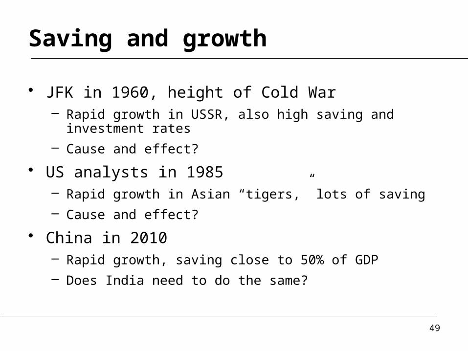
Saving and growth
• JFK in 1960, height of Cold War – Rapid growth in USSR, also high saving and investment
rates – Cause and effect?
• US analysts in 1985– Rapid growth in Asian “tigers,” lots of saving – Cause and effect?
• China in 2010– Rapid growth, saving close to 50% of GDP – Does India need to do the same?
49

Saving and growth
• How does saving generate growth? • Critical to long-run performance?
50

The Solow Model
51

Solow model
• How it works – Saving finances capital accumulation– More capital leads to greater output – Impact eventually tails off: diminishing marginal
product of capital
52

Convergence?Log of Real Per Capita GDP (PPP, 2005 Chained US$)
19501953
19561959
19621965
19681971
19741977
19801983
19861989
19921995
19982001
20042007
20106
7
8
9
10
11
Canada France Italy Japan UK US China India Poland Thailand
Uganda
Source: Penn World Tables 7.053

India
• Saving and investment rates well below China• How important? • Experiments with Solow model
– Benchmark: start up and see where GDP goes – Raise saving rate – Introduce productivity growth
• What has the biggest impact?
54

India
• Solow model inputs (estimates for 2010) – GDP: 3.87 trillion 2005 USD – K: 5.78 trillion 2005 USD – L: 0.450 billion people – A: how do we compute this? – s: 0.25 – delta: 0.06
• Experiments – Raise s
55

What have we learned?
• Solow model– Saving-finances increases in capital
– Convergence property: growth eventually stops
– Conclusion: capital not the key to sustained growth
– Value: tool for exploring growth of emerging economies
• What are we missing? – TFP growth
56

For the ride home
57


![Production function [ management ]](https://img.pdfslide.net/doc/110x75/55561ba3d8b42ae0238b5119/production-function-management-.jpg)

