EUR 23303 EN - 2007

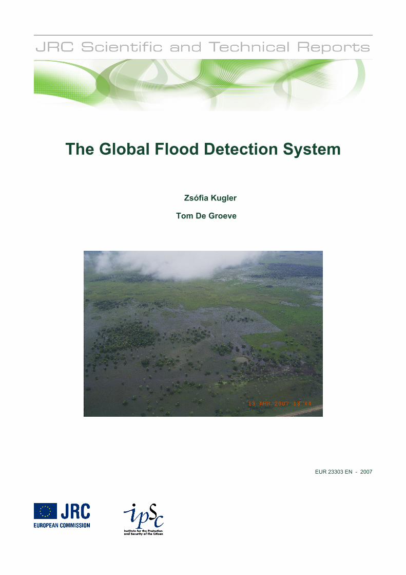
The Global Flood Detection System

Zsófia Kugler

Tom De Groeve

2

The Institute for the Protection and Security of the Citizen provides research-based, systems-oriented support to EU policies so as to protect the citizen against economic and technological risk. The Institute maintains and develops its expertise and networks in information, communication, space and engineering technologies in support of its mission. The strong cross-fertilisation between its nuclear and non-nuclear activities strengthens the expertise it can bring to the benefit of customers in both domains. European Commission Joint Research Centre Institute for the Protection and Security of the Citizen Contact information Address: CCR – TP267, Via Fermi 2749, 21020 Ispra, Italy E-mail: tom.de-groeve@jrc Tel.: +39-0332786340 Fax: +39-0332785154 http://ses.jrc.it http://www.jrc.cec.eu.int Legal Notice Neither the European Commission nor any person acting on behalf of the Commission is responsible for the use which might be made of this publication.

Europe Direct is a service to help you find answers to your questions about the European Union

Freephone number (*):

00 800 6 7 8 9 10 11

(*) Certain mobile telephone operators do not allow access to 00 800 numbers or these calls may be billed. A great deal of additional information on the European Union is available on the Internet. It can be accessed through the Europa server http://europa.eu/ JRC 44149 EUR 23303 EN ISSN 1018-5593 Luxembourg: Office for Official Publications of the European Communities © European Communities, 2007 Reproduction is authorised provided the source is acknowledged Printed in Italy

Content State of the art overview ....................................................................................................................... 5

Water surface change detection ............................................................................................................ 6

Site selection ......................................................................................................................................... 9

Source data ........................................................................................................................................... 9

Signal processing ................................................................................................................................ 11

Calibration of orbital gauging measures to in situ discharge measures ......................................... 11

Different sources of noise ............................................................................................................... 11

Spatial averaging ............................................................................................................................ 12

Temporal averaging ........................................................................................................................ 13

Flood thresholds ................................................................................................................................. 13

Humanitarian alert and information ................................................................................................... 14

GFDS operational use in Bolivia flood crisis, February - March 2007 ............................................. 15

GFDS operational use in the flood crisis West Africa 2007 .............................................................. 18

Introduction ........................................................................................................................................ 20

List of detected flood events .............................................................................................................. 21

Automatic matching of detected events and flood databases ............................................................. 39

Validation of major flood events ........................................................................................................ 21

Selection of major flood events for the period 2002-2007 ............................................................. 21

Manual check-up ............................................................................................................................ 23

Automatic quality check ..................................................................................................................... 26

Annex ................................................................................................................................................. 39

Annex 1: Automatic matching ....................................................................................................... 39

Error of omission ............................................................................................................................ 40

Annex 2: Results in a spatial context of the manual check-up ....................................................... 40

Annex 3: multidimensional analysis of parameter matrix .............................................................. 42

4

Abstract A methodology for satellite based flood detection developed (Brakenridge et al, 2007) at Dartmouth Flood Observatory (DFO) was modified at the Joint Research Centre (JRC) of the European Commission and implemented on an automatic operational basis. The technique uses AMSR-E passive microwave remote sensing data of the descending orbit, H polarization, 36 GHz band which is sensitive to water surface changes. The sensor revisits every place on Earth once per day and can therefore provide a daily temporal resolution. Sensor data is available 24 hours after acquisition. Thresholding the signal of water surface change allows the detection of riverine inundation events.

The comparison of gauging and satellite measurements show a significant correlation in the increase of river discharge on-site and changes in the observed signal of the sensor. Thus the technique for the detection of flood events in ungauged and inaccessible remote river channels is feasible from space.

A procedure chain was developed at the JRC to automatically acquire and process the remotely sensed data in real time on an operational basis. After the validation of the satellite based Global Flood Detection System (GFDS) the remotely observed flood events are to be integrated into the Global Disaster Alert and Coordination System (www.gdacs.org/floods) including the estimation of its humanitarian impact. GDACS is running at the JRC providing near real-time alerts about humanitarian and natural disasters around the world and tools to facilitate response coordination, including news and maps.

Introduction Of all natural disasters the floods are most frequent (46%) and cause most human suffering and loss (78% of population affected by natural disasters). They occur twice as much and affect about three times as many people as tropical cyclones. While earthquakes kill more people, floods affect more people (20000 affected per death compared to 150 affected per death for earthquakes) (OFDA/CRED, 2006). A study of the United Nations University (2004) shows that floods impact over half a billion people every year worldwide and might impact two billion by 2050, of which a disproportionate number live in Asia (44% of all flood disasters worldwide and 93% of flood-related deaths in the decade 1988-1997). According to a 2003 report of the World Water Council, flood and drought losses increased globally ten-fold (inflation corrected) over the second half of the 20th century, to a total of around US$ 300 billion in the 1990s. Since 2002, losses are estimated at US$ 96 billion (OFDA/CRED, 2006). In general on third of humanitarian aid goes to flood related disasters and the European Commission alone has spent €36 million on floods since 2002 (excluding funds for the tsunami of 2004)1.

Notwithstanding the seriousness of the socio-economic consequences of floods, there is at present no global system for their prediction nor even for consistent identification of flood events. Currently floods are not monitored systematically in all countries let alone globally. Less than 60% of the runoff from the continents is monitored at the point of inflow in the ocean, and the distribution of runoff within the continent is even less monitored (Bjerklie et al., 2003 and Fekete et al., 1999). Most international water management groups underline the need for core hydrological data. However monitoring stations around the world are decreasing in the past decades and decreasing number of stage records available (Calmant, 2006). A large set of river discharge data is collected by the Global Runoff Data Centre (GRDC) in the framework of international hydrological networks from in situ gauging stations with near global coverage (Figure 1). However, such internationally shared runoff data are usually provided as monthly mean values and not daily values in near-real time. Daily discharge data is only provided for the locations marked with blue dots.

5

Figure 1. Best on-site gauging discharge stations around the globe collected at GRDC. Only Blue stations are currently active.

Filling this lack of information, the Joint Research Centre (JRC) of the European Commission together with the Dartmouth Flood Observatory (DFO) joined forces to set up a Global Flood Monitoring System (GFDS). The aim of GFDS is to provide satellite based flow information around the globe substituting the missing on-site gauging in many parts of the world.

State of the art overview Most developed countries have reasonably sophisticated flood-prediction systems which are based on models using real-time reporting of extreme precipitation and other surface meteorological variables from in situ, radar and, in some cases, satellite observations (Bates and De Roo, 2000; Beven and Kirkby, 1979; De Roo, Wesseling and Van Deurzen, 2000; Galland, Goutal and Hervouet, 1991; Horritt and Bates, 2001). Such sophistication does not extend, however, to the developing world. For instance, in the Mozambique floods of 2000, only a handful of precipitation stations in the country were reporting over the WMO Global Telecommunication System—a number that would have made predictive modeling used in most flood-prediction systems in the developed world unfeasible to implement (Lettenmaier, De Roo and Lawford, 2006).

If floods can not be forecasted on a global scale, they may be detected in near-real time. Recent availability of daily satellite observations can provide the mean to do so. Barrett (1998) and others have shown that hydrographic data can be obtained from satellite sensors. However, most studies are restricted by the use of satellite resources not enabling daily monitoring.

The use of sensors in the visible or infrared portion of the spectrum is limited due to cloud cover. The microwave portion of the spectrum is not restricted by cloud cover. Early work on active (Smith, 1997) and passive (Sippel, Hamilton, Melack and Choudhury, 1994) microwave sensors for flood monitoring could not rely on satellites with daily revisit times. Since 1997 a set of new generation microwave instruments has been launched with improved performance and daily revisit capability. One of these, the Advanced Microwave Scanning Radiometer - Earth Observing System (AMSR-E) instrument on board of the NASA EOS Aqua satellite (launched in 2002), also has an extremely efficient data distribution mechanism making the data available for public download only hours after their acquisition. The US National Snow and Ice Data Center (NSIDC) provides preliminary swath data within 16 to 72 hours after acquisition on board. Since its launch in 2002, researchers looked at using there data for soil moisture monitoring (Njoku, Jackson, Lakshmi, Chan and Nghiem, 2003), rainfall monitoring (Hossain and Anagnostou, 2004) and flood forecasting (Bindlish, Crow and Jackson, 2004; Lacava, Cuomo, Di Leo, Pergola, Romano and Tramutoli, 2005), but not flood detection.

6

Methodology

Water surface change detection The Global Flood Detection System (GFDS) aims to provide a systematic detection of riverine flooding around the world. The techniques modifies the methodology first developed at the Dartmouth Flood Observatory (DFO) (Brakenridge et al., 2005) to monitor river sites and detect flooding by using the microwave radiation difference of land and water. Brackenridge et al. (2005) developed a method for daily monitoring of river systems around the globe based on AMSR-E data Figure 2.: AMSR-E passive microwave satellite data used for detecting floods on a global scale. They demonstrate that, using a methodology first developed for wide-area optical sensors (Al Khudhairy, Leemhuis et al., 2002; Brakenridge, Nghiem, Anderson and Mic, 2007), AMSR-E can measure river discharge changes and river ice status.

The modified methodology uses the 36GHz H-polarization band of the descending (nightly) orbit of AMSR-E with a footprint size of approximately 8x12km, available in the level 2A product (Ashcroft, 2003). Night time radiation is more stable than day time, for this reason only descending swaths of the sensor were used.

Figure 2.: AMSR-E passive microwave satellite data used for detecting floods on a global scale

The aim of the method is to detect water surface area change or, in other words, observe riverine inundation increase (land cover change) of a flood event from passive microwave sensor. Due to the different thermal inertia and emission properties of land and water the observed microwave radiation in general accounts for a lower brightness temperature (Tb) for water and higher for land (Figure 3). This makes it possible to detect inundation change of a river site in a sub-pixel dimension since most of the observed river channels are not as wide as the observation footprint.

To monitor flood events, the brightness temperature values for a number of observation sites over selected river sites were extracted from the AMSR-E satellite images. During a flood event – where water goes over bank – the increased water surface of the inundated area will cause a decrease in the brightness temperature (Tb) value detected by the satellite.

7

Figure 3. Methodology of the Global Flood Detection System (GFDS). Blue line is related to the wet/measurement pixel received over the river channel green line is related to the dry/calibration pixel not affected by the riverine

flooding.

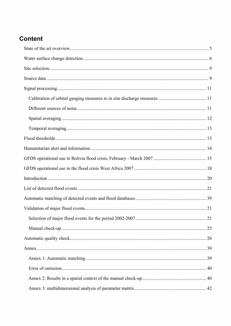
However, in spite of the great radiation dissimilarity of water and land cover, the raw brightness temperature observations are too noisy to reliably detect changes in surface water area. This is because brightness temperature measures are influenced by other factors such as physical temperature, permittivity1, surface roughness and atmospheric moisture. While the relative contribution of these factors cannot be measured, they are assumed to be constant over a larger area. Therefore, by comparing a “wet signal” received over a river channel of a potential inundation location with a “dry signal” without water cover the mentioned noise factors can be minimized. Thus normalisation of the wet signal by the dry observation was implemented where the brightness temperature values of the measurement/wet signal (Tbm) were divided by the calibration/dry observations (Tbc), referred to as M/C ratio:

M/C Ratio = Tbm / Tbc

Results of this kind (Figure 4) of calibration eliminates daily and seasonal temperature changes, soil moisture, vegetation influences by assuming that the wet and the dry location has the same properties except for the water surface extent.

1 Permittivity is a physical quantity that describes how an electric field affects and is affected by a dielectric medium, and is determined

by the ability of a material to polarize in response to the field, and thereby reduce the total electric field inside the material. Thus, permittivity relates to a material's ability to transmit (or "permit") an electric field.

8

Figure 4. M/C ratio (red line) minimises radiation variation originating from seasonal variations, soil moister, cloud cover and vegetation influences. M (Tbm) and C (Tbc) observations are blue and green lines respectively.

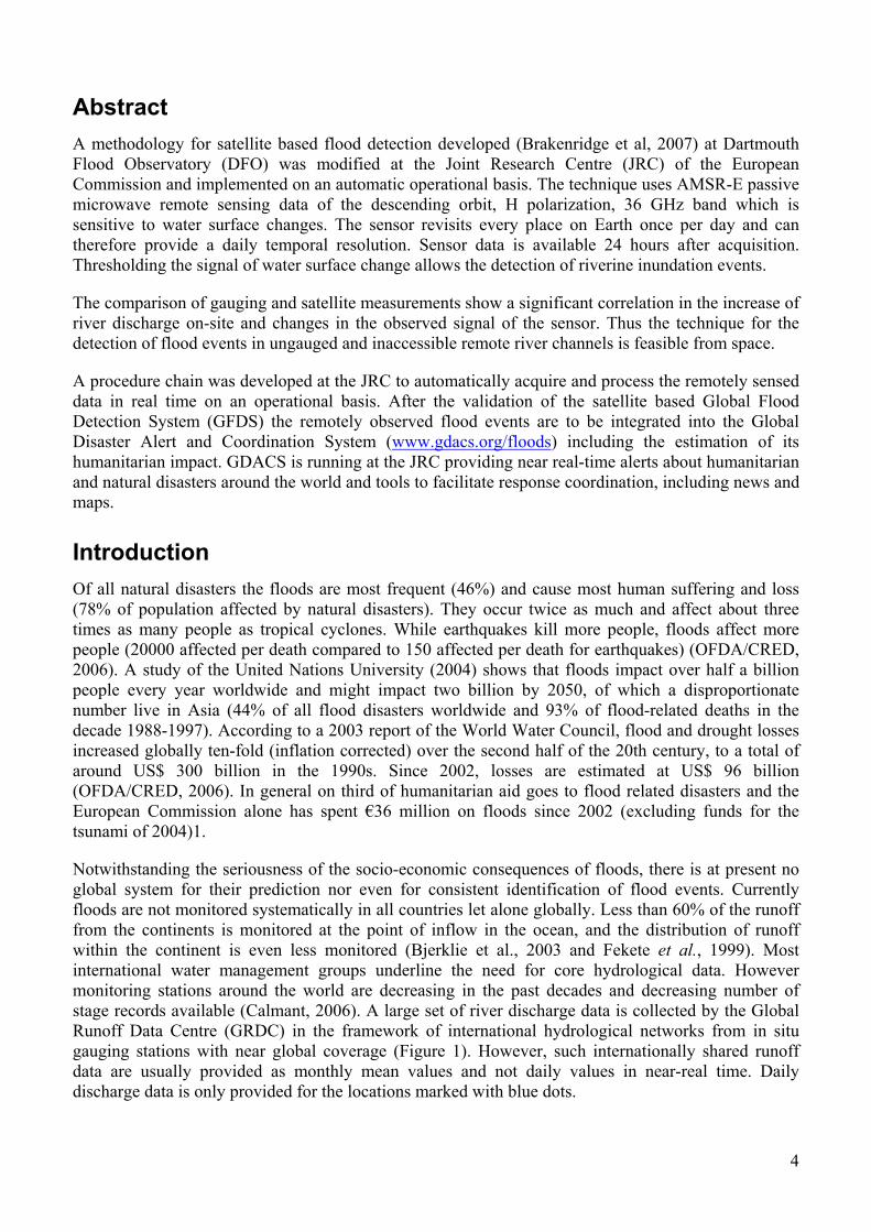
The time series of the M/C Ratio provides the basis of the space borne river gauging measurements and flood detection. During normal flow conditions water stays in-bank, dry and wet signals have nearly the same trend over time from space. As soon as the river floods and water goes over-bank, the proportion of water in the wet pixel greatly increases. The radiation received over the wet pixel lowers due to the lower emission of water while the dry pixel stays with minor variations constant. Consequently, there is a strong response in the M/C ratio in case of an inundation event (Figure 5).

Figure 5. Flood event detected on the River Indus in Pakistan in September 2003 from the M/C time series (red line).

FLOOD EVENT

9

Site selection Observation sites over river channels were set up around the globe. The list of sites initially monitored at DFO – about 100 locations – was at JRC extended to 2600 sites (Figure 7). Sites were selected if they were sensitive to surface water area change with increasing discharge. Selection was made manually at DFO based on historical flood events detected in MODIS low resolution images mounted on the same satellite platform Aqua. Calibration pixels were selected to be close to the measurement pixel – to enable the assumption of constant vegetation, soil moisture and meteorological conditions – but far enough not to be affected by flood inundation (Figure 6) (see also Brakenridge et al., 2007).

Figure 6. Footprint of the observation site over the Amazon River in Brazil. Blue dot refers to the footprint of the “wet” (measurement) pixel observation, green dot to the calibration “dry” pixel. (Background: Google Earth)

Observations and flood alerts are summarised in a database and visualised in the form of maps on the GFDS web page distributing information on the internet (www.gdacs.org/floods).

Figure 7. Space borne gauging stations around the globe monitored daily by GFDS

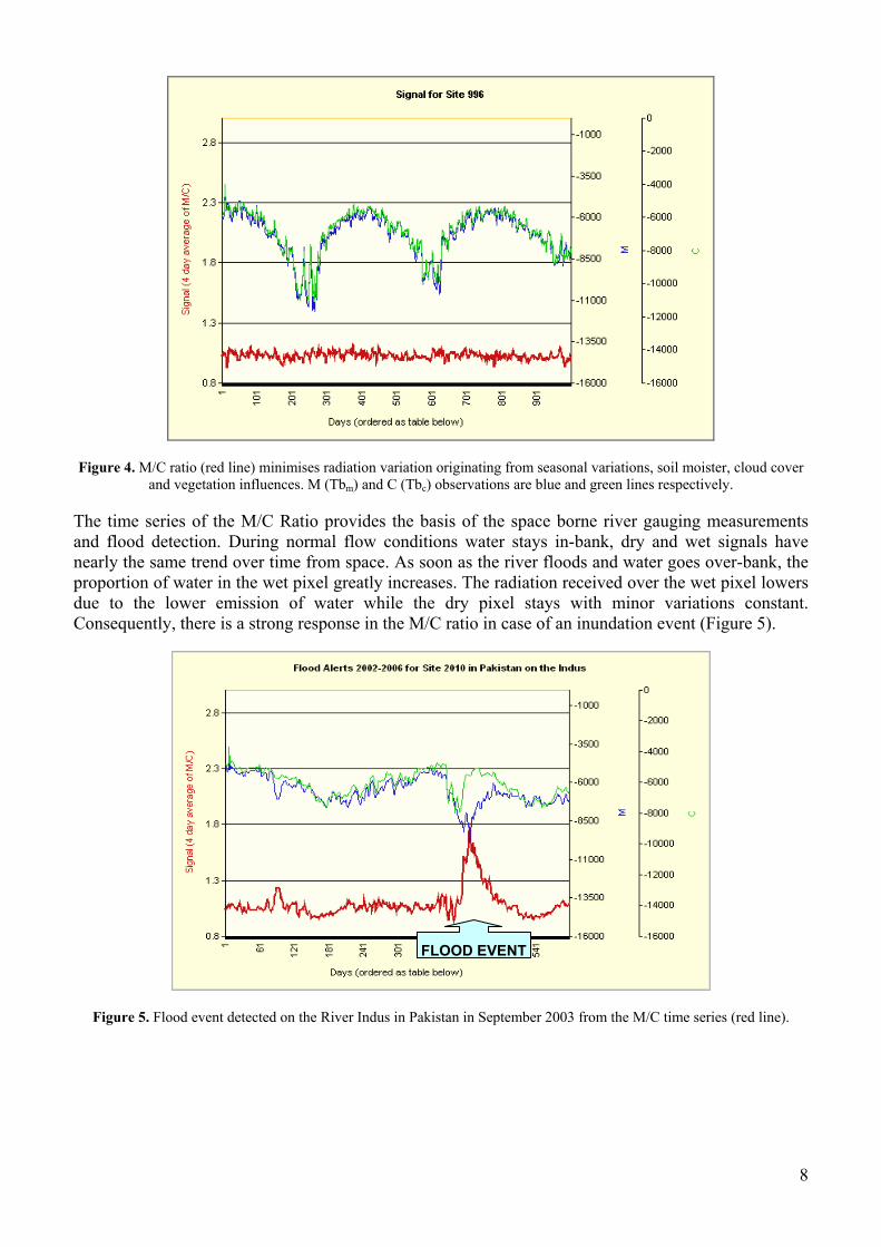
Source data The DFO methodology of Brakenridge et al. (2007) was developed with daily composite images. This was adapted at the JRC for the level 2A swath data of the AMSR-E sensor (Figure 8). The preliminary swath data used for the flood detection is provided by the National Snow and Ice Data Center (NSIDC) available within 12 hours after the acquisition on platform. DFO was using the level 3 global composite images with a 3 day lag which is much slower than the distribution of the swath data used at JRC for flood monitoring (Figure 8). In addition the swath has a higher spatial resolution, 10 km

10

instead of 25 km grid for the level 3 daily global composite. It is therefore more suitable for near-real time flood detection however its spatial properties defer from the gridded level-3 standard product.

Figure 8. Left image: near-real time swath data used at JRC; right image: daily composite used at DFO

In contrast to the mosaiced and gridded global composite data, the location of the observation in the swath data slightly varies from day to day. Consequently the distortion and scanning angle of the observation vary from day to day too. This means that the observations from different swaths – different days – for the same site are not necessarily easily comparable.

Not only the scanning angle but also the footprint size differs from swath to swath in the received signal. The two variations - the observation geometry and the spatial coverage - might cause a change in the percentile of water in the observation; as a result one observation might include more or less water. The influence of these parameters was not further investigated in detail however we note that it is one source for noise in the signal.

To select pixels covering the target observation site, a threshold of 0.1 decimal degrees (or about one pixel size) was used. Pixels are not considered where the centre is farther than this distance from the target observation site.

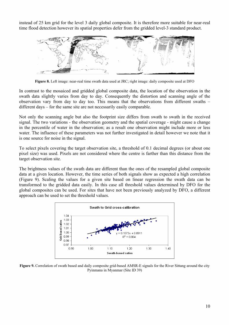
The brightness values of the swath data are different than the ones of the resampled global composite data at a given location. However, the time series of both signals show as expected a high correlation (Figure 9). Scaling the values for a given site based on linear regression the swath data can be transformed to the gridded data easily. In this case all threshold values determined by DFO for the global composites can be used. For sites that have not been previously analyzed by DFO, a different approach can be used to set the threshold values.

Figure 9. Correlation of swath based and daily composite grid-based AMSR-E signals for the River Sittang around the city Pyinmana in Myanmar (Site ID 39)

11

Signal processing

Calibration of orbital gauging measures to in situ discharge measures

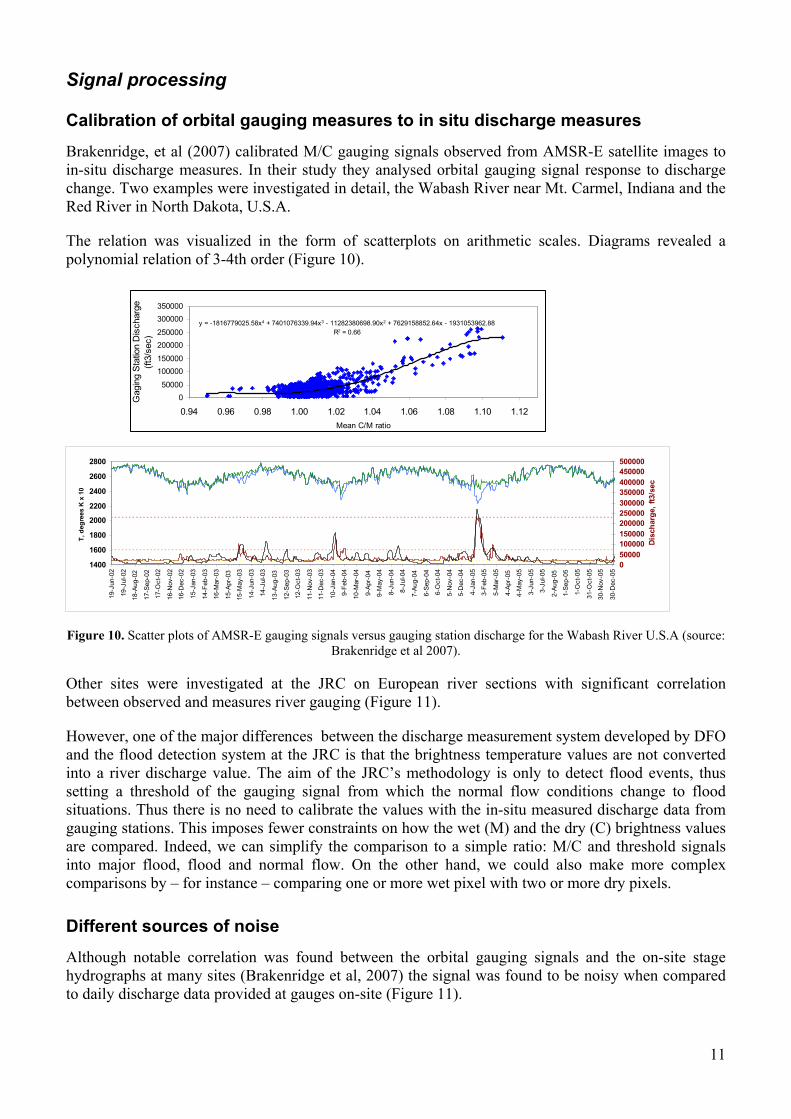
Brakenridge, et al (2007) calibrated M/C gauging signals observed from AMSR-E satellite images to in-situ discharge measures. In their study they analysed orbital gauging signal response to discharge change. Two examples were investigated in detail, the Wabash River near Mt. Carmel, Indiana and the Red River in North Dakota, U.S.A.

The relation was visualized in the form of scatterplots on arithmetic scales. Diagrams revealed a polynomial relation of 3-4th order (Figure 10).

Figure 10. Scatter plots of AMSR-E gauging signals versus gauging station discharge for the Wabash River U.S.A (source: Brakenridge et al 2007).

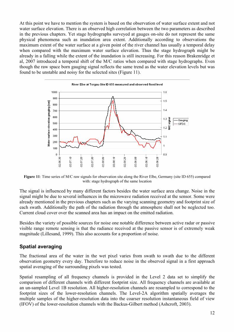
Other sites were investigated at the JRC on European river sections with significant correlation between observed and measures river gauging (Figure 11).

However, one of the major differences between the discharge measurement system developed by DFO and the flood detection system at the JRC is that the brightness temperature values are not converted into a river discharge value. The aim of the JRC’s methodology is only to detect flood events, thus setting a threshold of the gauging signal from which the normal flow conditions change to flood situations. Thus there is no need to calibrate the values with the in-situ measured discharge data from gauging stations. This imposes fewer constraints on how the wet (M) and the dry (C) brightness values are compared. Indeed, we can simplify the comparison to a simple ratio: M/C and threshold signals into major flood, flood and normal flow. On the other hand, we could also make more complex comparisons by – for instance – comparing one or more wet pixel with two or more dry pixels.

Different sources of noise

Although notable correlation was found between the orbital gauging signals and the on-site stage hydrographs at many sites (Brakenridge et al, 2007) the signal was found to be noisy when compared to daily discharge data provided at gauges on-site (Figure 11).

y = -1816779025.58x4 + 7401076339.94x3 - 11282380698.90x2 + 7629158852.64x - 1931053962.88R2 = 0.66

050000

100000150000

200000250000

300000350000

0.94 0.96 0.98 1.00 1.02 1.04 1.06 1.08 1.10 1.12Mean C/M ratio

Gag

ing

Stat

ion

Dis

char

ge

(ft3/

sec)

1400

1600

1800

2000

2200

2400

2600

2800

19-J

un-0

2

19-J

ul-0

2

18-A

ug-0

2

17-S

ep-0

2

17-O

ct-0

2

16-N

ov-0

2

16-D

ec-0

2

15-J

an-0

3

14-F

eb-0

3

16-M

ar-0

3

15-A

pr-0

3

15-M

ay-0

3

14-J

un-0

3

14-J

ul-0

3

13-A

ug-0

3

12-S

ep-0

3

12-O

ct-0

3

11-N

ov-0

3

11-D

ec-0

3

10-J

an-0

4

9-Fe

b-04

10-M

ar-0

4

9-Ap

r-04

9-M

ay-0

4

8-Ju

n-04

8-Ju

l-04

7-Au

g-04

6-Se

p-04

6-O

ct-0

4

5-N

ov-0

4

5-D

ec-0

4

4-Ja

n-05

3-Fe

b-05

5-M

ar-0

5

4-Ap

r-05

4-M

ay-0

5

3-Ju

n-05

3-Ju

l-05

2-Au

g-05

1-Se

p-05

1-O

ct-0

5

31-O

ct-0

5

30-N

ov-0

5

30-D

ec-0

5

T, d

egre

es K

x 1

0

050000100000150000200000250000300000350000400000450000500000

Dis

char

ge, f

t3/s

ec

12

At this point we have to mention the system is based on the observation of water surface extent and not water surface elevation. There is an observed high correlation between the two parameters as described in the previous chapters. Yet stage hydrographs surveyed at gauges on-site do not represent the same physical phenomena such as inundation area extent. Additionally according to observations the maximum extent of the water surface at a given point of the river channel has usually a temporal delay when compared with the maximum water surface elevation. Thus the stage hydrograph might be already in a falling while the extent of the inundation is still increasing. For this reason Brakenridge et al, 2007 introduced a temporal shift of the M/C ratios when compared with stage hydrographs. Even though the raw space born gauging signal reflects the same trend as the water elevation levels but was found to be unstable and noisy for the selected sites (Figure 11).

Figure 11: Time series of M/C raw signals for observation site along the River Elbe, Germany (site ID 655) compared with: stage hydrograph of the same location

The signal is influenced by many different factors besides the water surface area change. Noise in the signal might be due to several influences in the microwave radiation received at the sensor. Some were already mentioned in the previous chapters such as the varying scanning geometry and footprint size of each swath. Additionally the path of the radiation through the atmosphere shall not be neglected too. Current cloud cover over the scanned area has an impact on the emitted radiation.

Besides the variety of possible sources for noise one notable difference between active radar or passive visible range remote sensing is that the radiance received at the passive sensor is of extremely weak magnitude (Lillesand, 1999). This also accounts for a proportion of noise.

Spatial averaging

The fractional area of the water in the wet pixel varies from swath to swath due to the different observation geometry every day. Therefore to reduce noise in the observed signal in a first approach spatial averaging of the surrounding pixels was tested.

Spatial resampling of all frequency channels is provided in the Level 2 data set to simplify the comparison of different channels with different footprint size. All frequency channels are available at an un-sampled Level 1B resolution. All higher-resolution channels are resampled to correspond to the footprint sizes of the lower-resolution channels. The Level-2A algorithm spatially averages the multiple samples of the higher-resolution data into the coarser resolution instantaneous field of view (IFOV) of the lower-resolution channels with the Backus-Gilbert method (Ashcroft, 2003).

13

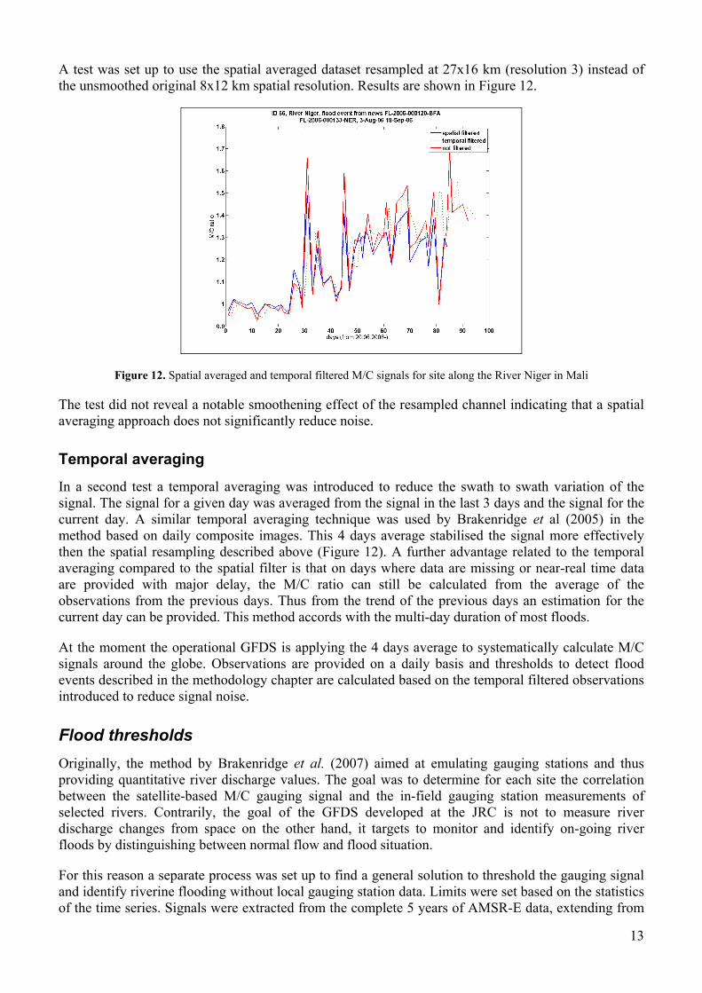
A test was set up to use the spatial averaged dataset resampled at 27x16 km (resolution 3) instead of the unsmoothed original 8x12 km spatial resolution. Results are shown in Figure 12.

Figure 12. Spatial averaged and temporal filtered M/C signals for site along the River Niger in Mali

The test did not reveal a notable smoothening effect of the resampled channel indicating that a spatial averaging approach does not significantly reduce noise.

Temporal averaging

In a second test a temporal averaging was introduced to reduce the swath to swath variation of the signal. The signal for a given day was averaged from the signal in the last 3 days and the signal for the current day. A similar temporal averaging technique was used by Brakenridge et al (2005) in the method based on daily composite images. This 4 days average stabilised the signal more effectively then the spatial resampling described above (Figure 12). A further advantage related to the temporal averaging compared to the spatial filter is that on days where data are missing or near-real time data are provided with major delay, the M/C ratio can still be calculated from the average of the observations from the previous days. Thus from the trend of the previous days an estimation for the current day can be provided. This method accords with the multi-day duration of most floods.

At the moment the operational GFDS is applying the 4 days average to systematically calculate M/C signals around the globe. Observations are provided on a daily basis and thresholds to detect flood events described in the methodology chapter are calculated based on the temporal filtered observations introduced to reduce signal noise.

Flood thresholds Originally, the method by Brakenridge et al. (2007) aimed at emulating gauging stations and thus providing quantitative river discharge values. The goal was to determine for each site the correlation between the satellite-based M/C gauging signal and the in-field gauging station measurements of selected rivers. Contrarily, the goal of the GFDS developed at the JRC is not to measure river discharge changes from space on the other hand, it targets to monitor and identify on-going river floods by distinguishing between normal flow and flood situation.

For this reason a separate process was set up to find a general solution to threshold the gauging signal and identify riverine flooding without local gauging station data. Limits were set based on the statistics of the time series. Signals were extracted from the complete 5 years of AMSR-E data, extending from

14

the launch of the system June 2002 to the present time. The download and processing of near-real time satellite data is automatic and the signal extraction is ongoing, extending the time series of the gauging signals and systematically updating their statistics every day.

River flooding is defined when the M/C ratio is higher then 80% of the signal’s cumulative frequency over the time series. Major flood is the 95% percentile (2 standard deviations), flood is the 80% percentile (1.5 standard deviations) and normal flow is below the 80% percentile of its cumulative histogram. These thresholds have been used in the rest of the paper.

Thresholds for extreme floods have not been finalized yet. However, in the past year, a threshold of 4 (orange) to 6 (red) standard deviations seem to correctly identify extreme floods, which are reported in the media. This needs to be confirmed with further research.

Humanitarian alert and information As with earthquakes and tropical cyclones, floods are only noteworthy for the humanitarian community if they disrupt or threaten to disrupt society significantly. Therefore, the detection of a new flood is not enough to launch a flood alert. The risk of disruption must be calculated, which is a combination of population affected, their vulnerability and the size of the flood. This is the purpose for the Global Disaster Alert and Coordination System (De Groeve, Vernaccini and Annunziato, 2006).

Currently, the floods detected by GFDS have not been systematically analyzed in this manner. However, the tools to do so are available. A GIS analysis of the region around the gauging site can provide relevant elements to estimate the impact of the flood. Population density, degree of slope, percentage of land used for agriculture and the density of infrastructure (roads and railways) can characterise the site as well as secondary risks such as landslides. A risk formula then must take into account the magnitude of the flood and the characteristics of the site to provide a risk score. The amount of agriculture land covered by the floods, combined with the time of year can indicate potential economic losses and possible need for food aid. Location of populated places and critical infrastructure, such as airports and main roads, can add value to the GDACS flood report.

Floods detected by GFDS are correlated with media articles. GFDS collects in automatic way relevant news articles (from the European Media Monitor; Best, Van Der Goot and De Paola, 2005).

15

Qualitative evaluation of the GFDS During the development of the Global Flood Detection System, the system was tested during several ad-hoc crisis responses to major flood events. At the beginning of 2007 GFDS was contributing to the flood disaster management in Bolivia and later that year in September to the extended flood crisis in West Africa. Both events and the contribution of GFDS are described in the next chapters.

GFDS operational use in Bolivia flood crisis, February - March 2007 The first operational test of GFDS was during the devastating flood crisis in Bolivia from the beginning of the year 2007 (glide number∗: FL-2007-000012-BOL). As described by observers on-site at the end of February “the flooding is reported to be the worst in 25 years, with 8 out of 9 departments of the country affected. On 28 February a government decree was issued declaring a (partial) national state of emergency. 43% (140 out of 327) of municipalities are in a state of emergency. An estimated 71,000 families (approx 355,000 persons) are affected. Santa Cruz and Beni regions are the worst affected. Several rivers are on a state of red alert.”

To support the ongoing flood event in February with spatial data (Figure 13) GDACS was providing information automatically. Using daily observations of AMSR-E images the Global Flood Detection System was providing information on river gauging along the flooded river sections. This was essential to get a situation overview since flood mapping from visible and infrared satellite resources like MODIS images were limited by cloud cover throughout February. Only partially cloud free scenes could be acquired at the end of the month processed by DFO. Maps were produced with the mapped flood extent and the detected flooded sites around the country at JRC.

Significant correlation was observed when comparing flood extent maps with the measurements of the relevant orbital gauging sites (Figure 13). Both are observing inundation extent changes. The basins of the River Mamore and River Grande were found to be the most affected areas of the country as seen on the situation overview from both sources.

∗ GLobal IDEntifier number (GLIDE) is a globally common unique ID code for disaster events issued by Asian Disaster Reduction

Center (ADRC)

16

Figure 13. Flood situation overview in Bolivia at the beginning March 2007. GFDS gauging sites are visualised in form of red or blue squares depending on the flow level of the site. The size of the dot refers to the duration of the event measured in days. The larger the dot the longer the observed event at a given site. Two gauging measures are attached to the map. In

the diagram red line refers to the threshold of the flood alert. Mapped extent of the flooded areas is visualised with light blue area along the flooded rivers. Extent was delivered by DFO from MODIS images.

An interactive map of the current flow situations was set up on the home page showing the gauging sites along flooded rivers outputting their current status of flow level. The map was automatically updated with the latest data downloaded and processed daily.

In this flooding emergency event the temporal resolution of AMSR-E flood observations was higher then the one of the flood maps derived from optical systems. A great advantage of using passive microwave system compared with other satellite resources like optical MODIS or active radar systems is to receive surface radiation on a daily global basis without the restriction of cloud coverage. While cloud cover or repetition time is limiting the use of the two latter satellite systems, GFDS has the advantage to provide a situation overview on a daily basis.

To enlarge the spatial extent of the space-borne gauging observations over the effected area new observation sites were set up along the flooded River Mamore, Rio Guapore, San Martin, Yapacani, Itonasmas, Grande and tributaries.

As a test for GFDS’s performance for spatially continuous observations along a river channel, new orbital observation sites were defined every 50 km along the most affected river basin of the Rio Mamore. Attached to the measurement sites only one calibration site was defined over the whole reach (Figure 14).

17

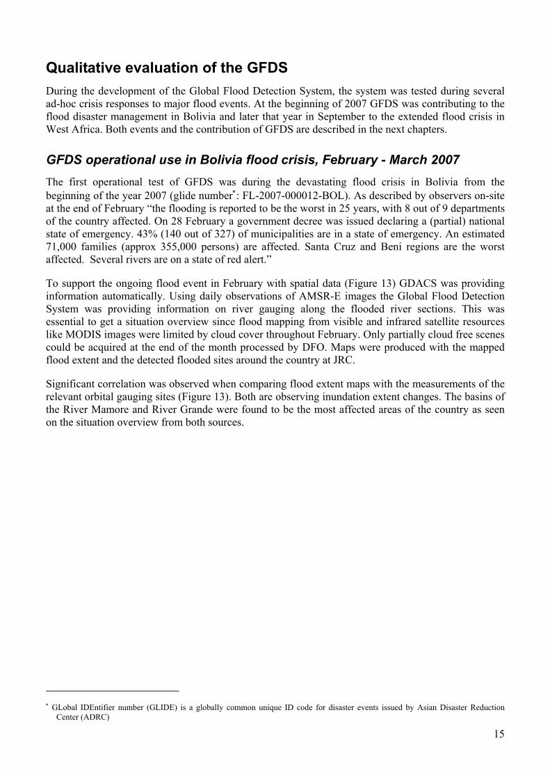
Figure 14. Location of orbital river gauging sites (yellow dots numbered sequentially) set during the flood emergency in Bolivia overlaid with the flood map derived from MODIS images (dark blue areas). Background: GTOPO elevation model.

With the new observation sites, the AMSR-E observations were providing a better temporal resolution with a high spatial sampling along the Rio Mamore when compared with optical low-resolution satellite systems. A situation overview of flow conditions in the whole river basin could be provided every day. Information was updated with the latest satellite data regardless of the cloud cover conditions.

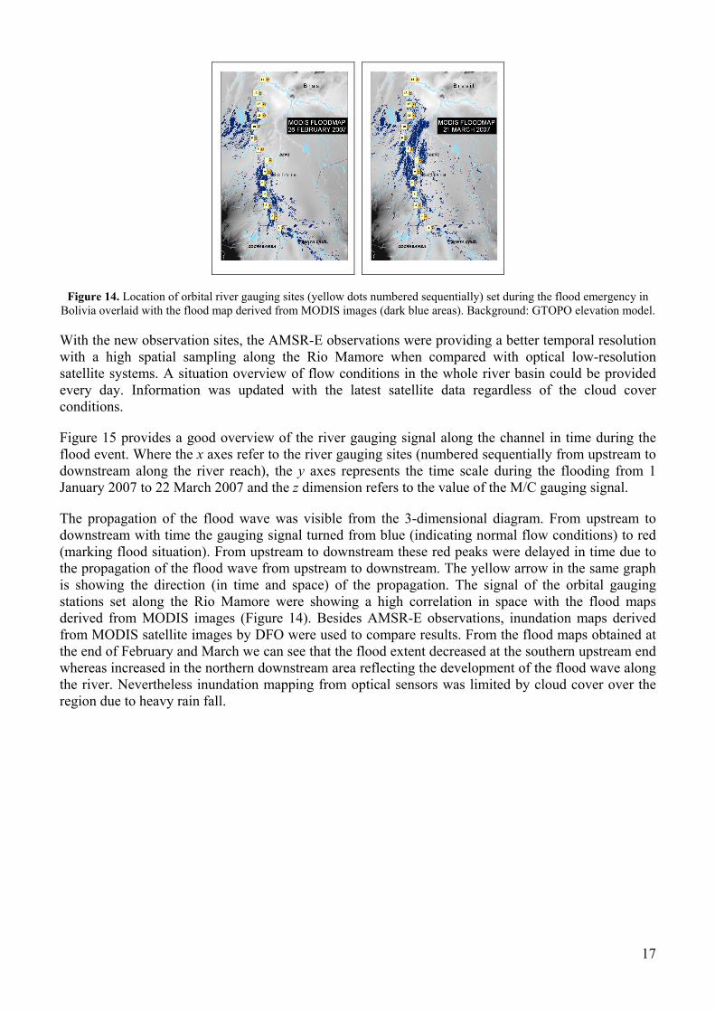
Figure 15 provides a good overview of the river gauging signal along the channel in time during the flood event. Where the x axes refer to the river gauging sites (numbered sequentially from upstream to downstream along the river reach), the y axes represents the time scale during the flooding from 1 January 2007 to 22 March 2007 and the z dimension refers to the value of the M/C gauging signal.

The propagation of the flood wave was visible from the 3-dimensional diagram. From upstream to downstream with time the gauging signal turned from blue (indicating normal flow conditions) to red (marking flood situation). From upstream to downstream these red peaks were delayed in time due to the propagation of the flood wave from upstream to downstream. The yellow arrow in the same graph is showing the direction (in time and space) of the propagation. The signal of the orbital gauging stations set along the Rio Mamore were showing a high correlation in space with the flood maps derived from MODIS images (Figure 14). Besides AMSR-E observations, inundation maps derived from MODIS satellite images by DFO were used to compare results. From the flood maps obtained at the end of February and March we can see that the flood extent decreased at the southern upstream end whereas increased in the northern downstream area reflecting the development of the flood wave along the river. Nevertheless inundation mapping from optical sensors was limited by cloud cover over the region due to heavy rain fall.

18

Figure 15. Three dimensional graph of the flood propagation along the Rio Mamore from AMSR-E observations. X axes: orbital gauging stations along the river; y axes: time scale; z axes: M/C values. Yellow arrow refers to the flood

propagation in space and time.

AMSR-E observations were able to provide a higher temporal resolution than optical images. This allows disasters managers to have a better situation overview of large floods in time and space.

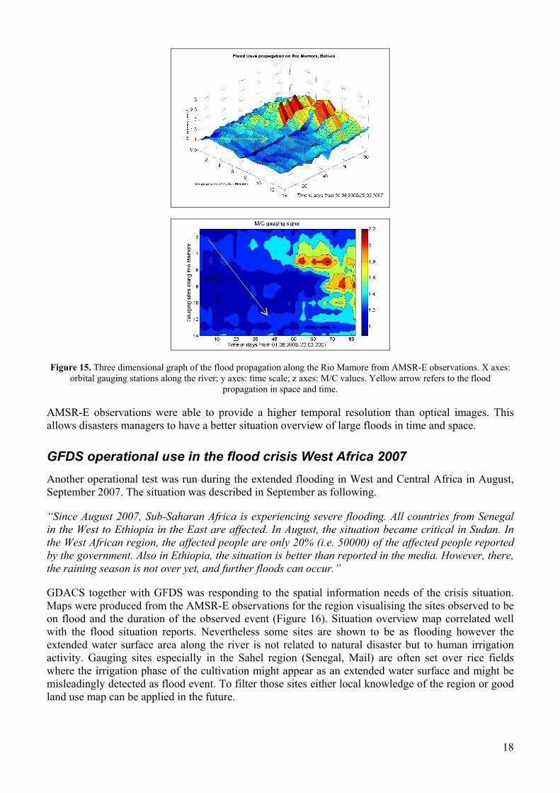
GFDS operational use in the flood crisis West Africa 2007 Another operational test was run during the extended flooding in West and Central Africa in August, September 2007. The situation was described in September as following.

“Since August 2007, Sub-Saharan Africa is experiencing severe flooding. All countries from Senegal in the West to Ethiopia in the East are affected. In August, the situation became critical in Sudan. In the West African region, the affected people are only 20% (i.e. 50000) of the affected people reported by the government. Also in Ethiopia, the situation is better than reported in the media. However, there, the raining season is not over yet, and further floods can occur.”

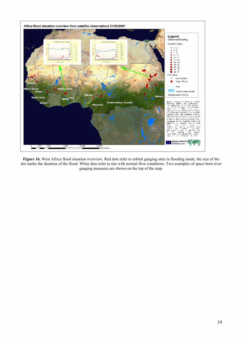
GDACS together with GFDS was responding to the spatial information needs of the crisis situation. Maps were produced from the AMSR-E observations for the region visualising the sites observed to be on flood and the duration of the observed event (Figure 16). Situation overview map correlated well with the flood situation reports. Nevertheless some sites are shown to be as flooding however the extended water surface area along the river is not related to natural disaster but to human irrigation activity. Gauging sites especially in the Sahel region (Senegal, Mail) are often set over rice fields where the irrigation phase of the cultivation might appear as an extended water surface and might be misleadingly detected as flood event. To filter those sites either local knowledge of the region or good land use map can be applied in the future.

19

Figure 16. West Africa flood situation overview. Red dots refer to orbital gauging sites in flooding mode, the size of the dot marks the duration of the flood. White dots refer to site with normal flow conditions. Two examples of space born river

gauging measures are shown on the top of the map.

20

Quantitative evaluation of the GFDS

Introduction To determine the level of normal flow or flood in a river section, a threshold is set for the cumulative histogram of the complete 4 years historical time series of AMSR-E signals. At the moment a river flood is detected when M/C signal is higher then the 80% cumulative frequency of the histogram of the time series.

This method is not necessarily appropriate for all observed sites. Some sites will have a different threshold value, some sites can have a threshold function over time (e.g. seasonal variation) and some sites can have signals that are not correlated with flood events at all. Therefore, site by site validation is extremely important to “graduate” a site as working in the GFDS.

To validate results different validation strategies could be applied for different sites. Rivers can be classified into gauged and ungauged regions. For gauged river sites AMSR-E observations are easier to validate: hydrological measurements of either water surface elevation gauging or discharge measurements can be correlated to AMSR-E signals directly. Of course, care has to be taken with comparing water elevation with flood extent.

However, most river systems are ungauged and their validation is more difficult. For ungauged river systems known flood events may help to confirm or disprove observed inundation signals derived from satellite data. Several databases exist on flood events around the world. The following list contains those downloaded and processed ones: CRED EM-DAT2, GLIDE 3, ECHO project database, OCHA Financial Tracking System4, DFO5. In most databases, inundation events are recorded with date, duration, and country. Unfortunately, the location and river basin are not recorded in all databases.

Based on the merging of these different flood databases in several steps an automatic procedure was set up to check the performance of the gauging signals observed from the AMSR-E images and the feasibility of flood detection from the observations. In a first step flood events derived from the physical observations were automatically matched up with the events of the database. Because of vague description of flood locations and dates in the databases, results were not satisfying.

Therefore, a selection was made of the major flood events of each year and the selected ones were manually matched up based on the location and the date with the detected flood events. As a result gauging sites were classified in different categories considering their performance in flood detection. Reliable signals were distinguished from noisy observations not appropriate for flood detection purposes. To extend measurement of signal performance from the small sample of manually checked sites to all observed gauging sites statistical parameters were derived for the complete time series of the signal. Using those statistical measurements a classification was made automatically to distinguish sites that can be reliably used for flood detection from those whose signal is too noisy to perform flood detection.

2 http://www.em-dat.net/disasters/list.php 3 http://www.glidenumber.net/glide/public/search/search.jsp 4 http://ocha.unog.ch/fts2/pageloader.aspx?page=emerg-emergencies&section=ND&year=2006 5 http://www.dartmouth.edu/%7Efloods/Archives/index.html

21

List of detected flood events Flood alerts derived from the AMSR-E gauging observations were converted into a list of detected flood events (Figure 17). An event was defined as a period during which a site has continuous flood or major flood alerts with no gap longer than 3 days. The database table of detected flood events contains information for:

- Site information (ID, Country, River) - Starting/ending day of the event - Duration - Gap

0

2000

4000

6000

8000

10000

12000

14000

16000

Rus

sia

USA

Chi

na

Aus

tralia

Bra

zil

Indi

a

Arg

entin

a

Can

ada

Indo

nesi

a

Mex

ico

Fran

ce

Bol

ivia

Thai

land

Phili

ppin

es

Nig

eria

Ukr

aine

Tanz

ania

Moz

ambi

que

Suda

n

Paki

stan

Viet

nam

Nr o

f obs

erve

d flo

od e

vent

s

Figure 17. Number of observed flood events from AMSR-E satellite images

Validation of major flood events

Selection of major flood events for the period 2002-2007

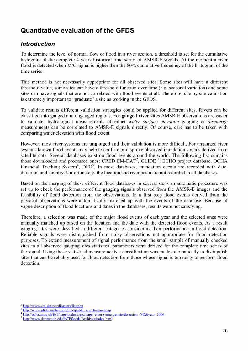
It is planned to integrate GFDS into GDACS as a physical measure of the flood hazard around the globe. Combining it with the vulnerability of the affected area GDACS/GFDS will provide the information in the future on potential humanitarian impact in order t o support disaster management, coordination and response. To validate the results of the GFDS several selected events were checked manually. The manual validation included the selection and check-up of major disaster events. The events to be analysed were selected according to their severity based on their humanitarian impact and damage. From the news based global disaster database of the Research on the Epidemiology of Disasters (CRED) (http://www.em-dat.net) maintained at the University of Louvain, 10 major flood events were selected each year reaching from the start of GFDS observations in 2002 till recently. The selection of the major events for a given year was done manually according to the number of deaths; the number of affected people and last but not least the estimated cost of damages and affected area of the disaster.

22

In the review of Guha-Sapir et al (2004) a summary is given on the number of flood events per territory (Figure 18) and the affected number of inhabitants (Figure 19) from news based sources. The first 15 major crises related to inundations from both statistical viewpoints are clearly concentrated in countries such as China, India and the territories of SE Asia annually hit by monsoonal rainfall.

Mean annual number of victims of flood and related disasters per 100,000 inhabitants: 1999 - 2003 by country and territory

0.00

2 000.00

4 000.00

6 000.00

8 000.00

10 000.00

12 000.00

Cam

bodia

China

Swaziland

Vietnam

Lao

Mozam

bique

India

Thailand

Sri

World

Botsw

ana

Malaw

i

Honduras

Sudan

Zambia

Somalia

Figure 18. Mean annual number of victims of flood and related disasters per 100,000 inhabitants in the period 1999-2003 registered by CRED6

Total number of flood and related disasters: 1999 - 2003By country and territory

0

10

20

30

40

50

60

China

Indonesia

India

USA

Colom

bia

Thailand

France

Philippines

Russian

Brazil

Vietnam

Iran

Nigeria

Afghanistan

Ethiopia

Mexico

Figure 19. Total number of victims of flood and related disasters per in the period 1999-2003 registered by CRED

Following this trend to choose the 10 major flood events every year from 2002 until the present time there was a manual selection based on the description above that resulted in 58 flood events in 23 different countries on the 4 major continents. The selected events are summarised in Figure 20 by the number of events by country. The trend of the last 10 years CRED recorded disasters (Figure 19) and the 58 selected major events of the last 6 years (Figure 20) show a significant correlation. Most flood events were selected from India, China, Bangladesh and Ethiopia. The same trend is visible on the GFDS observed flood events (Figure 19) where India, Indonesia and China were in the first 10 courtiers where most events were detected. USA and Russia were not considered in the validation process since external humanitarian aid is usually not needed to support their flood emergencies.

6 http://www.em-dat.net/disasters/list.php

23

Some events were included in the validation from Europe where regular gauging measurements are available, enabling the more precise recording of the arrival time of the flood wave at a given location along the river thus the more exact definition of the starting and ending date of the disaster.

Number of major flood events by country selected for the periode 2002-2007

0

2

4

6

8

10

12

14

Indi

a

Chi

na P

Rep

Bang

lade

sh

Ethi

opia

Indo

nesi

a

Col

ombi

a

Hun

gary

Nep

al

Pak

ista

n

Serb

ia M

onte

negr

o

Thai

land

Boliv

ia

Cam

bodi

a

Fran

ce

Ger

man

y

Hai

ti

Iran

Isla

m R

ep

Keny

a

Mal

aysi

a

Moz

ambi

que

Rom

ania

Rus

sia

Sri L

anka

Vie

t Nam

(bla

nk)

Figure 20. Number of the 10 major floods per year by country selected for GFDS validation

Manual validtaion

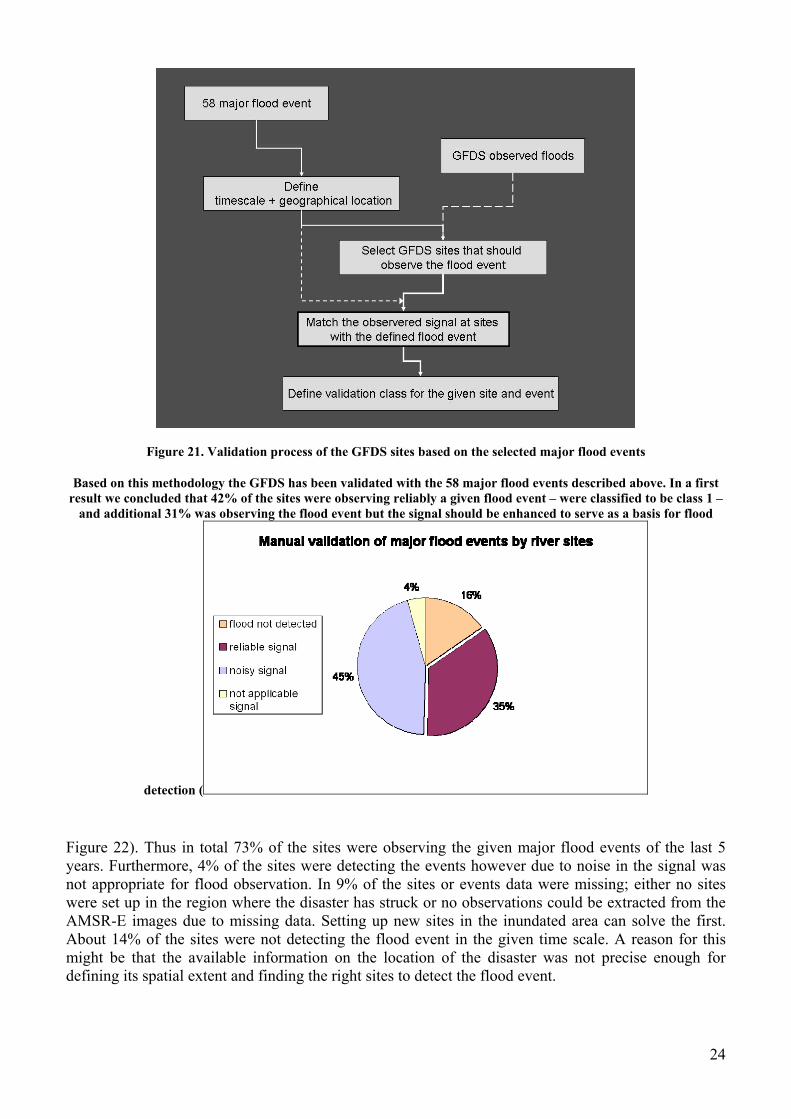
A validation process was set up to manually match the selected 58 major flood events from the CRED database with the GFDS observed flood events (Figure 21). In a first step the geographical location and the time scale of the major floods were allocated. The location was extracted from flood maps of DFO or descriptions of administrative areas or river names mentioned in the disaster databases. Flood maps have the disadvantage that due to cloud cover in some cases mapping cannot provide a complete overview of the inundated area. Descriptions given in the databases are lacking to give a precise location of the disaster. Based on these locations the orbital gauging sites were extracted that should have been observing the events. The signal time series for those selected sites were analysed in order to match flood alerts with the known major events. Depending on the quality of the observation and the time series of the selected sites, different classes of validation outcome were set up to measure their performance in detecting flood events.

Three classes were defined to estimate the quality of flood detection at a given location. Best sites were those where the flood event appeared as a significant increase in the signal well delineable from the average of its time series. These sites were marked as validation class 1. Class 2 was categorised when the increase in the signal was enabling the observation of the flood event however it was difficult to delineate from its average since due to noise in its time series. In those cases no clear events could be distinguished from the noise of the signal. Class 3 was set up for those sites where the signal was so noisy that it was not possible to derive flood events from it. Whereas the last will not improve, class 2 can still be used in the future for flood detection however with some restriction and modification. Sites that did not detect floods were marked as class 0 and sites that had no data in the selected timescale or sites were missing spatial location were marked as class 5.

24

Figure 21. Validation process of the GFDS sites based on the selected major flood events

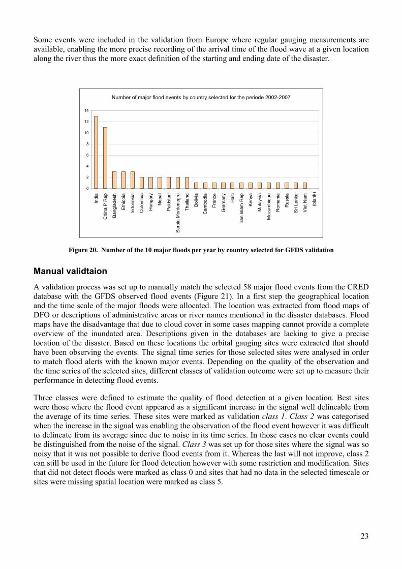
Based on this methodology the GFDS has been validated with the 58 major flood events described above. In a first result we concluded that 42% of the sites were observing reliably a given flood event – were classified to be class 1 –

and additional 31% was observing the flood event but the signal should be enhanced to serve as a basis for flood

detection (

Figure 22). Thus in total 73% of the sites were observing the given major flood events of the last 5 years. Furthermore, 4% of the sites were detecting the events however due to noise in the signal was not appropriate for flood observation. In 9% of the sites or events data were missing; either no sites were set up in the region where the disaster has struck or no observations could be extracted from the AMSR-E images due to missing data. Setting up new sites in the inundated area can solve the first. About 14% of the sites were not detecting the flood event in the given time scale. A reason for this might be that the available information on the location of the disaster was not precise enough for defining its spatial extent and finding the right sites to detect the flood event.

25

Therefore not taking in account the data missing we can conclude that a significant majority, 80% of the sites were detecting well the flood event however only 20% of the signals were not reliably or did not detect the flood event. Results are further described in a spatial context in annex 2.

Figure 22. Validation results per observation site detecting major flood events

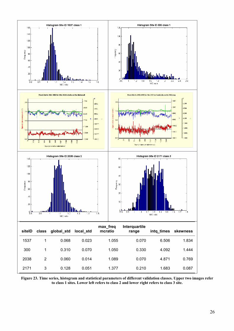
Different validation classes have different signal properties (Figure 23). As mentioned before ideally class 1 time series should have a significant signal increase in case a flood event occurs. Class 2 should have and increase in its signal but due the noise normal flow conditions are difficult to derive from the flood conditions. Class 3 signals are not used for flood detection due to their bad performance and high signal noise.

26

siteID class global_std local_std max_freq mcratio

Interquartilerange intq_times skewness

1537 1 0.068 0.023 1.055 0.070 6.506 1.834

300 1 0.310 0.070 1.050 0.330 4.092 1.444

2038 2 0.060 0.014 1.089 0.070 4.871 0.769

2171 3 0.128 0.051 1.377 0.210 1.683 0.087

Figure 23. Time series, histogram and statistical parameters of different validation classes. Upper two images refer to class 1 sites. Lower left refers to class 2 and lower right refers to class 3 site.

27

Automatic quality check An investigation was performed to find an automatic procedure to distinguish between the different signal quality classes. The test was based on the training sample of the selected and manually validated major flood events along the affected sites. Different statistical methods were investigated to evaluate the performance of different sites. In a first approach the histogram of the classes was visualised and analysed then various statistical parameters were used to describe the different forms and behaviour of their histograms.

The histogram of various validation classes shows a clear difference in their time series (Figure 23). Generally class 1 histograms can be described as having a non symmetrical, non Gaussian distribution with a strong positive skewness and a clear peak that is related to the average signal value. As mentioned before class 1 sites should have ideally a stable signal around the average – the Gaussian mid-part of the histogram - and extreme values well driveable from the average that is represented by the long thin tail to the right from the histogram peak. On the contrary class 2 histograms have a more symmetric distribution without a great difference between the average and the outlier values that makes it difficult to distinguish flood events from normal flow conditions. Class 3 sites, compared to any of the other classes ,have a histogram with a much wider standard deviation and with no clear extreme values, which makes the detection of events unfeasible.

To describe the different shapes of the histograms and to separate them into classes main statistical parameters were analysed in a second step (Figure 23). Besides the mean and spread depicted by their standard deviation – which were already calculated as a statistical parameter for the individual sites – various statistical descriptors were computed for the distribution. Since the mean of the data often does not represents the peak value of the histogram a separate calculation was done do get the most frequent M/C ratio category that is related to the maximum number of records in the frequency table. This varies from 1.76 to 0.7348 depending on the average difference between the M and the C values throughout its time series. Still on its own this parameter cannot tell the difference between good and bad sites.

Standard deviation is sensitive to extreme values and for this reason interquartile range was considered as an additional measure of spread in the histogram. Interquartile range is an indicator of dispersion without being much influenced by outliers. This parameter showed a better separation of the different time series classes then the standard deviation. While standard deviation varied from 0.57 to 0.02; interquartile range had a maximum of 0.95 and a minimum of 0.02. However taking the example of site 1537 and site 2038 neither dispersion measures did give a satisfactory and reliable estimate to distinguish between good and bad sites. Since the difference between the extreme values and the average is of more importance to derive flood events in a future step the symmetry or asymmetry in its distribution was investigated.

A calculation was run to find the number of interquartile ranges between the peak of the histogram (the maximum frequency ratio) and the greatest outlier (the maximum value of the histogram). The calculation was found to define the tail to the right in the histogram in other words the difference between the extreme values and the average. The higher the value the further the extreme values are separated from the mean, thus can better recognise events from their time series. Still if we compare site 300 and site 2038 neither does this measure give a good definition of class 1 and class 2 sites.

The result was particularly sensitive to extreme values thus another parameter was calculated to define the shape and the symmetry of the histogram. To measure the asymmetry of the probability distribution of the values, the skewness of the distribution was calculated. Concerning the examples shown in Figure 23. skewness seemed to be the most efficient way to distinguish between the classes. However, the results were not satisfactory when exploring the entire population of all sites.

28

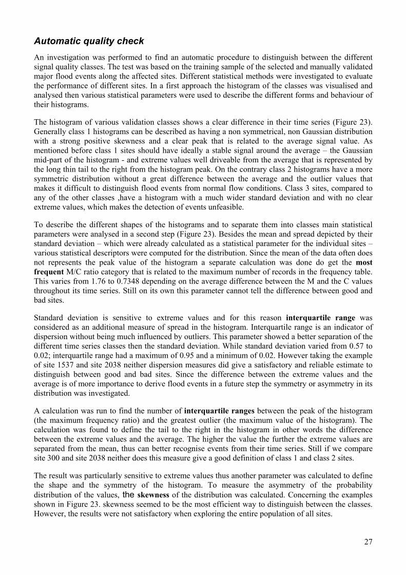
None of the aforementioned statistical parameters seems to provide a good basis for classification. For this reason further investigation was run using bivariate methods to classify the whole population. Scatter plots of different parameter combinations were visualised and analysed. To set an example interquartile range was plotted against skewness to get a visual picture of their relationship. The points trend to cluster along the axes (Figure 24) without having a clear difference between class 1 and class 2 sites. Yet the training data shows that this bivariate analysis did not get us nearer to a satisfactory classification strategy.

Figure 24. Scatter plot of the two variables skewness and interquartile range. The upper figure refers to training sample of the manual validation lower plot refers to all observed sites.

In a further step a multidimensional matrix was set up from all the statistical parameters that were calculated for the manually validated sites. Results are discussed in annex 3. So far the above mentioned methods using static statistical measures did not provide a sufficient solution in defining a clear division between class 1 and class 2 sites. For this reason an investigation was run to include the dynamics of the time scale in the analyses. A moving time window of 10 days was used to consider the dynamics of the signal. A comparison was done based on the static/global statistical parameter calculated for the whole signal as one unit and on the statistical parameter calculated in the 10 days local moving windows averaged over the time series. The best parameter to describe the difference between the two populations of different classes seemed to be the combination of the local and the global standard deviation. The training sample was first visualised in a 2 dimensional scatter plot to get an assessment of their relationship.

29

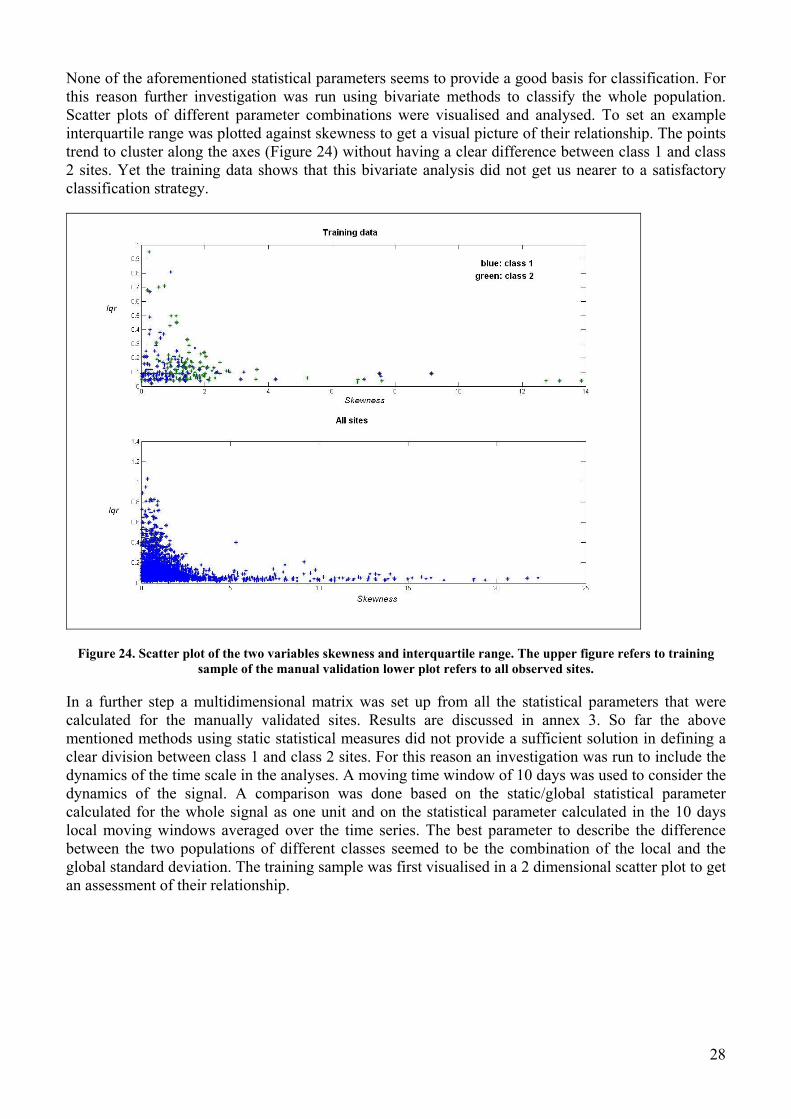
Figure 25. Scatter plot of the global and local standard deviation for the population of the manually validated sites. Numbering refers to validation classes. Linear margin is represented by green line.

The population of class 1 and class 2 sites were clustering around a linear line however class 1 sites were having lower local values (y values) related to global (x values) ones (Figure 25). This indicates the lower signal noise of class 1 time series compared to class 2 signals. Even though the two populations do not clearly separate the trend shows that the two classes can be distinguished by drawing a linear margin between them to distinguish. All sites under this linear border can be classified as class 1 sites and all sites above this boundary can be regarded as class 2 sites. This linear margin was empirically set between the two classes and was defined as the following:

y = 0.2312 * x + 0.015

Where:

x = is the global standard deviation

y = is the average of the local standard deviations calculated for every 10 days

After a manual check it seemed that sites near to the origin independent from the linear margin drawn between the two classes were found to be performing well. These are sites where neither the local nor the global standard deviation was high. For this reason another rule was added to the linear margin. All sites were considered as being good ones where:

x < 0.05 and y < 0.2312 * 0.05 + 0.015

Using this empirical function 86% of the class 1 sites of the training sample were classified correctly and 36% of the class 2 sites were not correctly distinguished from the rest of the population.

Table 1. Validation classes distinguished by the empirical function.

Validation Class Good bad

1 84% 16%

2 39% 61%

3 40% 60%

CLASS 1

CLASS 2

30

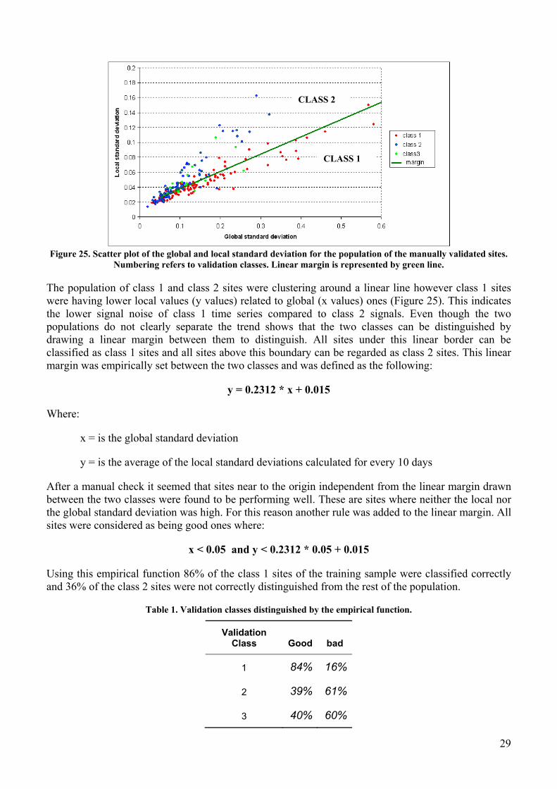
Applying this formula to the whole population with a probability of 73% we can distinguish automatically good sites from not functionally appropriate ones. Based on the validation sites, these were flagged good/reliable sites and bad/not working sites (Figure 26). The latter ones were taken out from the operational alerting system but their observations were not removed from the daily measurements.

Figure 26. Global coverage of observed sites taken out from observation after validation process.

In summary, a fully automatic processing chain has been set up to detect flood events. The system can be extended with a minor manual interaction any time by taking new river sites into observation. However, to validate its applicability we established an automatic procedure that can distinguish with 73% certainty well working new orbital gauging sites from the ones that can not to be applied for flood detection.

31

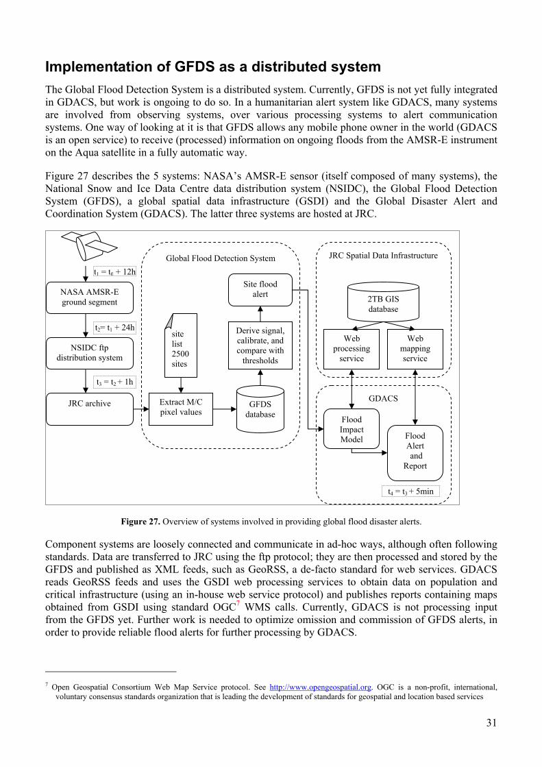
Implementation of GFDS as a distributed system The Global Flood Detection System is a distributed system. Currently, GFDS is not yet fully integrated in GDACS, but work is ongoing to do so. In a humanitarian alert system like GDACS, many systems are involved from observing systems, over various processing systems to alert communication systems. One way of looking at it is that GFDS allows any mobile phone owner in the world (GDACS is an open service) to receive (processed) information on ongoing floods from the AMSR-E instrument on the Aqua satellite in a fully automatic way.

Figure 27 describes the 5 systems: NASA’s AMSR-E sensor (itself composed of many systems), the National Snow and Ice Data Centre data distribution system (NSIDC), the Global Flood Detection System (GFDS), a global spatial data infrastructure (GSDI) and the Global Disaster Alert and Coordination System (GDACS). The latter three systems are hosted at JRC.

Figure 27. Overview of systems involved in providing global flood disaster alerts.

Component systems are loosely connected and communicate in ad-hoc ways, although often following standards. Data are transferred to JRC using the ftp protocol; they are then processed and stored by the GFDS and published as XML feeds, such as GeoRSS, a de-facto standard for web services. GDACS reads GeoRSS feeds and uses the GSDI web processing services to obtain data on population and critical infrastructure (using an in-house web service protocol) and publishes reports containing maps obtained from GSDI using standard OGC7 WMS calls. Currently, GDACS is not processing input from the GFDS yet. Further work is needed to optimize omission and commission of GFDS alerts, in order to provide reliable flood alerts for further processing by GDACS.

7 Open Geospatial Consortium Web Map Service protocol. See http://www.opengeospatial.org. OGC is a non-profit, international,

voluntary consensus standards organization that is leading the development of standards for geospatial and location based services

GDACS

JRC Spatial Data Infrastructure Global Flood Detection System

NASA AMSR-E ground segment

NSIDC ftp distribution system

t1 = t0 + 12h

t2= t1 + 24h

JRC archive

t3 = t2 + 1h

site list 2500 sites

Extract M/C pixel values

GFDS database

Derive signal, calibrate, and compare with

thresholds

Site flood alert 2TB GIS

database

Web processing

service

Web mapping service

Flood Impact Model Flood

Alert and

Report

t4 = t3 + 5min

32

On average, the time between the flood event and the flood alert is around 36 hours. Since the satellite passes most locations on earth once per day, the delay between flood (t0) and observation (t1) is between 0 and 24 hours, with an average of 12 hours. From the time of observation to publication on the NSIDC ftp site (t2) takes on average 24 hours (based on 1 year operation of GFDS). A download at JRC of one AMSR-E track file takes on average 10 minutes, but since multiple tracks are often published at once, the download time averages to about 1 hour. Files are available at JRC for processing (t5) on average 25 hours after observation or between 25 and 49 hours after a (sudden) flood event. Processing at JRC is a matter of minutes. Data for 2500 pixels are extracted from the data files in less than 10 seconds and inserted in a MySQL database. The flood signal (C/M ratio, with 4 day average) is recalculated with the new data and XML feeds are published dynamically. For other disasters, GDACS routinely checks data sources each 5 minutes and would do so too for GFDS. GDACS impact models typically run in less than 1 minute.

One disadvantage of distributed systems is that the whole system is depending on composing systems. For example, GFDS is completely dependent on a single data provider, NSIDC, with which no formal service level agreement has been signed at this point in time. Furthermore, the system is also dependent on data from a single satellite, with a limited life time. To make GFDS more robust, more data sources and data providers must be brought in, making the system even more distributed.

Figure 28. Floods appearing in the media and GFDS observations for the River Pungue in Mozambique

33

Discussion and suggestions for future work At the moment around 2500 river sites on 1400 different rivers are monitored with the GFDS systematically. The monitoring locations can be extended any time with minor manual work. As soon as the location is defined and new latitude longitude coordinates are added to the observations, the system automatically starts to acquire data for the new site from the date it was added to GFDS. The extraction of historical data for the new site is not automatic yet. This procedure including the extraction of historical data was done during the flood crisis in Bolivia. Nevertheless only discrete observations were set along the Rio Mamore where major problems occurred.

A small test was run to analyse the applicability of the method in a spatial context. To use the entire image as one single unite not only to extract discrete observations from the data. Primarily results showed that it is difficult to distinguish seasonal variability from changes related to flooded areas. However we leave this to future investigation.

On the other hand the location the calibration/dry pixel could be also investigated in more detail. From several different locations around the wet pixel a searching algorithm could be set to find the most optimal location for the calibration observation. In an optimal approach, the time series of the calibration observation should have the same trend like the measurement pixel. Only in case of a flood event should the two signals significantly differ.

Noisy sites should be filtered with the automatic procedure of the validation process described. This should enable to cut noisy, not applicable signal from the observations thus to get a more reliable basis to issue flood alerts. The function of alerts can be also subject to further investigations. High signal outliers that did not occur yet in the time series consequently have a huge standard deviation are not investigated in detail yet.

On the other hand false alerts related to human irrigation are also to be minimised in the future. As described in the case of the West African flood crisis many sites are set over rivers where changes in the extent of water surfaces is not related to natural disasters but to human irrigation of rice fields along the river. However only knowledge based verification or high quality up-to-date land use maps can help to filter those sites out.

Another issue that could be subject of future investigation is the sensitivity of the model. A study could focus on the geometrical parameters of river channels where flood detection is feasible. Likewise, the minimum width of a channel could be analysed where GFDS is capable to observe inundation.

Another important topic to analyse is the connectivity, the topology of river reaches. They enhance the reliability of issued alerts countries are summarised. If a given proportion of river sites are detected to be flooded, alerts can be issued with a higher reliability then discrete observations. This is already implemented in the operational alerting. On the other hand a manual check of the alerted river sites is on-going. Sites that are on alert for a given day are summarised and checked manually every day to enhance the operational use of the system.

Currently, the method is based on data from a single instrument on a single satellite: the US/Japanese Advanced Microwave Scanning Radiometer – Earth Observation System (AMSR-E) on board of the Aqua satellite. However, the method can be modified to work with different data sources. Since the lifetime of AMSR-E is limited, new data sources must be considered for a sustainable system. Candidates are similar sensors, such as the European Microwave Radiometer (MWR) on board of ENVISAT, which records microwave radiation at similar frequency. Also active radar remote sensing can be considered. Work is ongoing between DFO and NASA to evaluate the use of QuickScat for flood detection. Furthermore, optical data can be considered in spite of their limitations by clouds.

34

Weather satellites have an acquisition frequency in the order of 30 minutes, which can improve flood detection in cloud free conditions. These possibilities need to be examined further.

Conclusions The Global Flood Detection System provides a systematic monitoring of ongoing flood events around the world updated every day. This fills the gap in lack of global, hydrological data collection. Especially remote not gauged regions could benefit from the GFDS providing information about current flow status. An overview of the flood situation in many flood emergencies is missing as experienced during the West Africa and Bolivia flood crises. The high revisit capability of the applied AMSR-E satellite system and the independency of cloud cover enable the technology to acquire information to meet the requirements of operational crisis response. This enables the system to serve as an alternative to flood mapping from optical or radar systems. However, the low pixel size can be a limiting factor in monitoring small narrow river reaches. In the future work is planned to investigate extending the methodology not only to individual observations but to spatial monitoring based on the whole satellite image as one unit.

The model can also be used to reconstruct historical flood events that were not recorded in a systematic way from the launch of the satellite system in 2002. Further, it can support the detection of seasonal flooding and reoccurring events that can be summarised in a form of a global flood disaster atlas.

The verification of the model results and the validation of the detected flood event were demonstrated in the report. An automatic procedure is now serving the basis of validation to filter the time series of not reliable observation site. Based on that the system can be extended at any time with new observation sites as mentioned in the discussion chapter and their applicability can be checked automatically. The validated flood detection system will be integrated shortly in the operational Global Disaster Alert and Coordination System (GDACS) issuing natural disaster alerts and their impact around the globe on an automatic 24/7 basis.

35

References

Alexei V. Kouraeva,b,*, Elena A. Zakharovab, Olivier Samainc, Nelly M. Mognarda, Anny Cazenavea: Ob’ river discharge from TOPEX/Poseidon satellite altimetry (1992–2002), Remote Sensing of Environment 93 (2004) 238– 245

Alsdorf, D.E., J. M. Melack, T. Dunne, L.A.K. Mertes, L.L. Hess, and L.C. Smith, Interferometric radar measurements of water level changes on the Amazon floodplain, Nature, 404, 174-177, 2000.

Ashcroft, P., and F. Wentz. 2003, updated daily. AMSR-E/Aqua L2A Global Swath Spatially-Resampled Brightness Temperatures (Tb) V001, January to October 2006. Boulder, CO, USA: National Snow and Ice Data Center. Digital media.

Ashcroft, P., and F. Wentz. 2003, updated daily. AMSR-E/Aqua L2A Global Swath Spatially-Resampled Brightness Temperatures (Tb) V001, June 2002 to recent. Boulder, CO, USA: National Snow and Ice Data Center. Digital media. (accessed 22 March 2007)

Ashcroft, P., and F. Wentz. 2003, updated daily. AMSR-E/Aqua L2A Global Swath Spatially-Resampled Brightness Temperatures (Tb) V001, June 2002 to recent. Boulder, CO, USA: National Snow and Ice Data Center. Digital media. (accessed 22 March 2007)

B.M. Fekete, C.J. Vorosmarty and W. Grabs, 1999. WMO-Global Runoff Data Center ReportWMO-Global Runoff Data Center Report 22 (1999) p. 114

Barrett, E., 1998. Satellite remote sensing in hydrometry. In: Ed, H. (Ed.), Hydrometry: Principles and Practices. Wiley, Chichester, UK, pp. 199–224.

Barrett, E., 1998. Satellite remote sensing in hydrometry. In: Ed, H. (Ed.), Hydrometry: Principles and Practices. Wiley, Chichester, UK, pp. 199–224.

Bates, P.D. and De Roo, A.P.J., 2000. A simple raster-based model for flood inundation simulation. Journal of Hydrology, 236: 54-77.

Bates, P.D., De Roo, A.P.J., 2000. A simple raster-based model for flood inundation simulation. Journal of Hydrology 236, 54–77.

Beven, K J and Kirkby, M J. 1979. A physically based variable contributing area model of basin hydrology Hydrol. Sci. Bull., 24(1), 43-69.

Birkett, C.M., Contribution of the TOPEX NASA radar altimeter to the global monitoring of large rivers and wetlands, Water Resources Research, 34, 1223-1239, 1998.

Bjerklie, D.M., S. L.Dingman, C. J. Vorosmarty, C. H. Bolster, R. G. Congalton: Evaluating the potential for measuring river discharge from space, Journal of Hydrology 278. (2003), pp. 17–38

Brakenridge, G. R. , Nghiem, S. V. , Anderson, E., Mic, R., 2006. Orbital Microwave Measurement of River Discharge and Ice Status, Water Resources Research, In press.

36

Brakenridge, G. R., and E. Anderson, 2006. Dartmouth Flood Observatory Active archive of large floods, 1985-present, edited by G. R. B. a. E. Anderson, Dartmouth College, Hanover, NH USA. , http://www.dartmouth.edu/~floods/

Brakenridge, G. R., S. V. Nghiem, E. Anderson, R. Mic, 2007, Orbital Microwave Measurement of River Discharge and Ice Status, Water Resources Research, In press

Brakenridge, G.R., Anderson, E., Caquard, S., 1985-2007, Flood Inundation Maps DFO, Dartmouth Flood Observatory, Hanover, USA, digital media, 2007 //www.dartmouth.edu/~floods/

Brakenridge, G.R., Anderson, E., Caquard, S., 2003, Flood Inundation Map DFO 2003-282, Dartmouth Flood Observatory, Hanover, USA, digital media, http://www.dartmouth.edu/~floods/2003282.html (accessed 22 March 2007)

Choudhury, B.J., 1989. Monitoring global land surface using Nimbus- 7 37 GHz data. Theory and examples. International Journal of Remote Sensing 10 (10), 1579–1605.

D.P. Lettenmaier, A. de Roo and R. Lawford, 200x. Towards a capability for global flood forecasting, Journal?

Darcy J., and Hofmann, C-A., 2003. “According to need? Needs assessment and decision-making in the humanitarian sector”, Humanitarian Policy Group Report 15, London: Overseas Development Institute

De Groeve, T., Ehrlich, D., 2002. DMA Earthquake Alert Tool, A decision support tool for humanitarian aid, Technical Note No. I.02.75, Institute for the Protection and the Security of the Citizen, Cybersecurity and New Technologies for Combating Frauds.

De Groeve, T., L. Vernaccini and A. Annunziato, 2006. Global Disaster Alert and Coordination System. In Proceedings of the 3rd International ISCRAM Conference, Eds. B. Van de Walle and M. Turoff,, Newark, pp.1-10.

De Roo, A.P.J., Wesseling, C.G., Van Deurzen, W.P.A., 2000. Physically based river basin modelling within a GIS: the LISFLOOD model. Hydrological Processes 14, 1981–1992.

Al-Khudhairy, D.H.A., Leemhuis, C., Hoffmann, V., Shepherd, I.M., Calaon, R., Thompson, J.R., Gavin, H., Papadimos, D. (2002) Monitoring wetland ditch water levels using Landsat TM and ground-based measurements, Photogrammetric Engineering and Remote Sensing 68 (8), pp. 809-818.

Elena A. Zakharova, Alexei V. Kouraev, Anny Cazenave, Frédérique Seyler: Amazon River discharge estimated from TOPEX/Poseidon altimetry, Surface Geosciences (Hydrology), 338 (2006) 188–196

European Commission Humanitarian Office, 2006 (Personal communication)

F. Frappart, J.M. Martinez, F. Seyler, J.G. Leon, A. Cazenave: Determination of the water volume variation in the Negro River sub-basin by combination of remote sensing and in-situ data, Remote Senssing of the Environment 99 (2005) 387–399.

Fekete, B.M., C.J. Vorosmarty and W. Grabs, 1999. WMO-Global Runoff Data Center ReportWMO-Global Runoff Data Center Report 22 (1999) p. 114

37

Galland, J.C., Goutal, N., Hervouet, J.-M., 1991. TELEMAC—a new numerical-model for solving shallow-water equations. Advances in Water Resources 14 (3), 138–148

GUHA-SAPIR., D. HARGITT, D. HOYOIS, Ph. (2004). Thirthy years of natural disasters 1974-2003: The numbers, Presses Universitaires de Louvain: Louvain-la Neuve. [ID n202]

H. Roux and D. Dartus, 2006. Use of parameter optimization to estimate a flood wave: Potential applications to remote sensing of rivers. Journal of Hydrology, Volume 328, Issues 1-2, 30 August 2006, Pages 258-266

Hess, L. L., Melack, J. M., Filoso, S. &Wang, Y. Delineation of inundated area and vegetation along the Amazon floodplain with SIR-C synthetic aperture radar. IEEE Trans. Geosci. Remote Sensing 33, 896-904 (1995).

Horritt, M.S. and Bates, P.D., 2001. Predicting floodplain inundation: raster-based modelling versus the finite-element approach. Hydrological Processes, 15(5): 825-842.

Koblinsky, C.J., R.T. Clarke, A.C. Brenner, and H. Frey, Measurement of river level variations with satellite altimetry, Water Resources Research, 6, 18391848, 1993.

Lillesand, T.M., Kiefer, R.W.: Remote sensing and image interpretation, 3 ed., John Wiley & Sons, Inc., 1994

M. Temimi, R. Leconte, F. Brissette, N. Chaouch: Flood and soil wetness monitoring over the Mackenzie River Basin using AMSR-E 37 GHz brightness temperature, Journal of Hydrology (2007) 333, 317– 328

M.S. Horritt , 2006. A methodology for the validation of uncertain flood inundation models, Journal of Hydrology 326 153–165

NASA , 2006. The Tropical Rainfall Measuring Mission (TRMM), on-line (http://trmm.gsfc.nasa.gov/), last access: 17.10.2006

Njoku, E., Koike, T., Jackson, T. J., & Paloscia, S. (2000). Retrieval of soil moisture from AMSR data. In P. Pampaloni, & S. Paloscia (Eds.), Microwave radiometry for remote sensing of earth’s surface and atmosphere (pp. 525– 533). Utrecht, The Netherlands7 VSP.

OFDA/CRED, 2006. “2005 disasters in numbers”, OFDA/CRED, http://www.em-dat.net (accessed 22 March 2007)

OFDA/CRED, 2006. “2005 disasters in numbers”, OFDA/CRED, http://www.em-date.net

Paul F. Hudsona,*, Rene´ R. Colditzb: Flood delineation in a large and complex alluvial valley, lower Pa´nuco basin, Mexico, Journal of Hydrology 280 (2003) 229–245

Rajat Bindlish, Thomas J. Jackson, Albin J. Gasiewski, Marian Klein, Eni G. Njoku: Soil moisture mapping and AMSR-E validation using the PSR in SMEX02 Remote Sensing of Environment 103 (2006) 127–139

RESPOND home page, www.respond.org

38

RESPOND home page, www.respond.org, 2006, (accessed 22 March 2007)

Roux H., and D. Dartus, 2006. Use of parameter optimization to estimate a flood wave: Potential applications to remote sensing of rivers. Journal of Hydrology, Volume 328, Issues 1-2, 30 August 2006, Pages 258-266

S. J. Sippel, S. K. Hamilton, J. M. Melack And E. M. M. Novo: Passive microwave observations of inundation area and the area/stage relation in the Amazon River foodplain, International Journal of Remote Sensing, 1998, vol. 19, no. 16, 3055 - 3074

Sippel, S.J., Hamilton, S.K., Melack, J.M., Choudhury, B.J., 1994. Determination of inundation area in the Amazon River floodplain using SMMR 37 GHz polarization difference. Remote Sensing Environment 48, 70–76.

Smith, L. C., 1997. Satellite remote sensing of river inundation area, stage, and discharge: A review. Hydrol. Processes 11, 1427-1439.

Smith, L. C., 1997. Satellite remote sensing of river inundation area, stage, and discharge: A review. Hydrol. Processes 11, 1427-1439.

Stéphane Calmant, Frédérique Seyler: Continental surface waters from satellite altimetry, 338 (2006) 1113–1122 Internal Geophysics (Space Physics)

Stippel, S.J., Hamilton, S.K., Melack, J.M., Choudhury, B.J., 1994. Determination of inundation area in the Amazon River floodplain using SMMR 37 GHz polarization difference. Remote Sensing Environment 48, 70–76.

T. Lacava, V. Cuomo, E. V. Di Leo, N. Pergola, F. Romano and V. Tramutoli, 2005. Improving soil wetness variations monitoring from passive microwave satellite data: The case of April 2000 Hungary flood , Remote Sensing of Environment, Volume 96, Issue 2, 30 May 2005, Pages 135-148

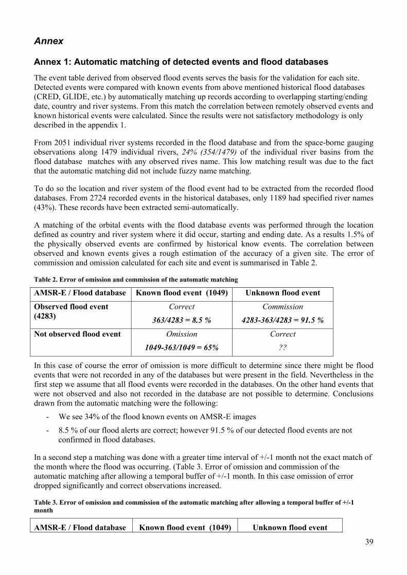
39

Annex

Annex 1: Automatic matching of detected events and flood databases

The event table derived from observed flood events serves the basis for the validation for each site. Detected events were compared with known events from above mentioned historical flood databases (CRED, GLIDE, etc.) by automatically matching up records according to overlapping starting/ending date, country and river systems. From this match the correlation between remotely observed events and known historical events were calculated. Since the results were not satisfactory methodology is only described in the appendix 1.

From 2051 individual river systems recorded in the flood database and from the space-borne gauging observations along 1479 individual rivers, 24% (354/1479) of the individual river basins from the flood database matches with any observed rives name. This low matching result was due to the fact that the automatic matching did not include fuzzy name matching.

To do so the location and river system of the flood event had to be extracted from the recorded flood databases. From 2724 recorded events in the historical databases, only 1189 had specified river names (43%). These records have been extracted semi-automatically.

A matching of the orbital events with the flood database events was performed through the location defined as country and river system where it did occur, starting and ending date. As a results 1.5% of the physically observed events are confirmed by historical know events. The correlation between observed and known events gives a rough estimation of the accuracy of a given site. The error of commission and omission calculated for each site and event is summarised in Table 2.

Table 2. Error of omission and commission of the automatic matching

AMSR-E / Flood database Known flood event (1049) Unknown flood event

Observed flood event (4283)

Correct

363/4283 = 8.5 %

Commission

4283-363/4283 = 91.5 %

Not observed flood event Omission

1049-363/1049 = 65%

Correct

??

In this case of course the error of omission is more difficult to determine since there might be flood events that were not recorded in any of the databases but were present in the field. Nevertheless in the first step we assume that all flood events were recorded in the databases. On the other hand events that were not observed and also not recorded in the database are not possible to determine. Conclusions drawn from the automatic matching were the following:

- We see 34% of the flood known events on AMSR-E images

- 8.5 % of our flood alerts are correct; however 91.5 % of our detected flood events are not confirmed in flood databases.

In a second step a matching was done with a greater time interval of +/-1 month not the exact match of the month where the flood was occurring. (Table 3. Error of omission and commission of the automatic matching after allowing a temporal buffer of +/-1 month. In this case omission of error dropped significantly and correct observations increased.

Table 3. Error of omission and commission of the automatic matching after allowing a temporal buffer of +/-1 month

AMSR-E / Flood database Known flood event (1049) Unknown flood event

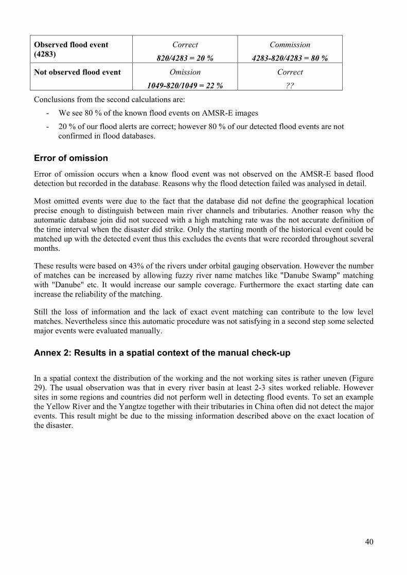
40

Observed flood event (4283)

Correct

820/4283 = 20 %

Commission

4283-820/4283 = 80 %

Not observed flood event Omission

1049-820/1049 = 22 %

Correct

??

Conclusions from the second calculations are:

- We see 80 % of the known flood events on AMSR-E images

- 20 % of our flood alerts are correct; however 80 % of our detected flood events are not confirmed in flood databases.

Error of omission

Error of omission occurs when a know flood event was not observed on the AMSR-E based flood detection but recorded in the database. Reasons why the flood detection failed was analysed in detail.

Most omitted events were due to the fact that the database did not define the geographical location precise enough to distinguish between main river channels and tributaries. Another reason why the automatic database join did not succeed with a high matching rate was the not accurate definition of the time interval when the disaster did strike. Only the starting month of the historical event could be matched up with the detected event thus this excludes the events that were recorded throughout several months.

These results were based on 43% of the rivers under orbital gauging observation. However the number of matches can be increased by allowing fuzzy river name matches like "Danube Swamp" matching with "Danube" etc. It would increase our sample coverage. Furthermore the exact starting date can increase the reliability of the matching.

Still the loss of information and the lack of exact event matching can contribute to the low level matches. Nevertheless since this automatic procedure was not satisfying in a second step some selected major events were evaluated manually.

Annex 2: Results in a spatial context of the manual check-up

In a spatial context the distribution of the working and the not working sites is rather uneven (Figure 29). The usual observation was that in every river basin at least 2-3 sites worked reliable. However sites in some regions and countries did not perform well in detecting flood events. To set an example the Yellow River and the Yangtze together with their tributaries in China often did not detect the major events. This result might be due to the missing information described above on the exact location of the disaster.

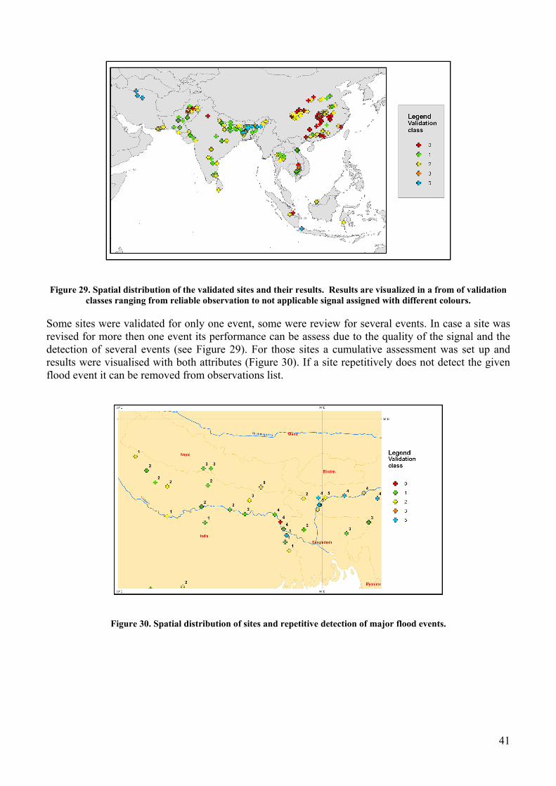
41

Figure 29. Spatial distribution of the validated sites and their results. Results are visualized in a from of validation classes ranging from reliable observation to not applicable signal assigned with different colours.

Some sites were validated for only one event, some were review for several events. In case a site was revised for more then one event its performance can be assess due to the quality of the signal and the detection of several events (see Figure 29). For those sites a cumulative assessment was set up and results were visualised with both attributes (Figure 30). If a site repetitively does not detect the given flood event it can be removed from observations list.

Figure 30. Spatial distribution of sites and repetitive detection of major flood events.

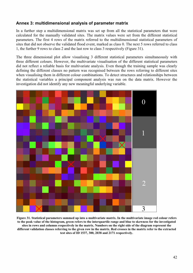
42

Annex 3: multidimensional analysis of parameter matrix

In a further step a multidimensional matrix was set up from all the statistical parameters that were calculated for the manually validated sites. The matrix values were set from the different statistical parameters. The first 4 rows of the matrix referred to the multidimensional statistical parameters of sites that did not observe the validated flood event, marked as class 0. The next 5 rows referred to class 1, the further 9 rows to class 2 and the last row to class 3 respectively (Figure 31).

The three dimensional plot allow visualising 3 different statistical parameters simultaneously with three different colours. However, the multivariate visualisation of the different statistical parameters did not reflect a reliable basis for multivariate analysis. Even though the training sample was clearly defining the different classes no pattern was recognised between the rows referring to different sites when visualising them in different colour combinations. To detect structures and relationships between the statistical variables a principal component analysis was run on the data matrix. However the investigation did not identify any new meaningful underlying variable.

Figure 31. Statistical parameters summed up into a multivariate matrix. In the multivariate image red colour refers to the peak value of the histogram, green refers to the interquartile range and blue to skewness for the investigated

sites in rows and columns respectively in the matrix. Numbers on the right side of the diagram represent the different validation classes referring to the given row in the matrix. Red crosses in the matrix refer to the extracted

test sites of ID 1537, 300, 2038 and 2171 respectively.

43

European Commission EUR 23303 EN – Joint Research Centre – Institute for the Protection and Security of the Citizen Title: The Global Flood Detection System Author(s): Zsófia Kugler, Tom De Groeve Luxembourg: Office for Official Publications of the European Communities 2007 – 63 pp. – 21 x 30 cm EUR – Scientific and Technical Research series – ISSN 1018-5593 Abstract

A methodology for satellite based flood detection developed at Dartmouth Flood Observatory (DFO) was modified at the Joint Research Centre (JRC) of the European Commission and implemented on an automatic operational basis. The technique is using AMSR-E passive microwave remote sensing data of the descending orbit, H polarization, 36 GHz band which is sensitive to water surface changes. The sensor revisits every place on Earth once per day and can therefore provide a daily temporal resolution. Sensor data is available 24 hours after acquisition. Thresholding the signal of water surface change allows the detection of riverine inundation events.

The comparison of in field gauging and satellite measurements show a significant correlation in the increase of river discharge on-site and changes at the observed signal of the sensor. Thus following the technique the detection of flood events in ungauged and inaccessible remote river channels is feasible from space.

A procedure chain was developed at the JRC to automatically acquire and process the remotely sensed data in real time on an operational basis. After the validation of the satellite based Global Flood Detection System (GFDS) the remotely observed flood events are to be integrated into the Global Disaster Alert and Coordination System (www.gdacs.org/floods) including the estimation of its humanitarian impact. GDACS is running at the JRC providing near real-time alerts about natural disasters around the world and tools to facilitate response coordination, including news and maps.

44

How to obtain EU publications Our priced publications are available from EU Bookshop (http://bookshop.europa.eu), where you can place an order with the sales agent of your choice. The Publications Office has a worldwide network of sales agents. You can obtain their contact details by sending a fax to (352) 29 29-42758.

45

The mission of the JRC is to provide customer-driven scientific and technical support for the conception, development, implementation and monitoring of EU policies. As a service of the European Commission, the JRC functions as a reference centre of science and technology for the Union. Close to the policy-making process, it serves the common interest of the Member States, while being independent of special interests, whether private or national.

A

A- B

B- XXXXX- LL- C