The Golem Group/University of California at Los Angeles ... Golem Group/University of California at Los Angeles Autonomous Ground Vehicle in the DARPA Grand Challenge ... and allows

The Golem Group/University ofCalifornia at Los Angeles

Autonomous Ground Vehicle inthe DARPA Grand Challenge

Richard Mason, Jim Radford, Deepak Kumar,Robert Walters, Brian Fulkerson,Eagle Jones, David Caldwell, Jason Meltzer,Yaniv Alon, Amnon Shashua, Hiroshi Hattori,Emilio Frazzoli, and Stefano SoattoThe Golem Group911 Lincoln Boulevard #7Santa Monica, California 90403

Received 13 December 2005; accepted 12 June 2006

This paper presents the Golem Group/University of California at Los Angeles entry tothe 2005 DARPA Grand Challenge competition. We describe the main design principlesbehind the development of Golem 2, the race vehicle. The subsystems devoted to obstacledetection, avoidance, and state estimation are discussed in more detail. An overview ofvehicle performance in the field is provided, including successes together with an analy-sis of the reasons leading to failures. © 2006 Wiley Periodicals, Inc.

1. OVERVIEW

The Golem Group is an independent team of engi-neers formed to build a vehicle for the 2004 DARPAGrand Challenge �DGC�. For the 2005 DARPA GrandChallenge, the Golem Group and the University ofCalifornia at Los Angeles �UCLA’s� Henry SamueliSchool of Engineering and Applied Science joinedforces to build a second autonomous vehicle, Golem2 �see Figure 1�. Performance highlights of this ve-hicle are summarized in Table I.

The aspect of the DGC was to require high-speedautonomous driving in the unstructured or semi-structured environment typical of rough desert trails.Global positioning system �GPS� waypoint followingwas necessary, but not sufficient, to traverse the route,

which might be partially obstructed by various ob-stacles. In order to have a good chance of completingthe course, vehicles needed to drive much faster, yethave a lower failure rate, than previously achieved inan off-road environment without predictable cues.High-speed driving over rough ground posed a vi-bration problem for sensors.

1.1. Relation to Previous Work

Prior to the DGC, unmanned ground vehicles haddriven at very high speeds in structured paved en-vironments �Dickmanns, 1997, 2004�. Other vehicleshad operated autonomously in unstructured off-road environments, but generally not at very highspeed. Autonomous Humvees using ladar �laser de-

• • • • • • • • • • • • • • • • • • • • • • • • • • • • • • •

Journal of Field Robotics 23(8), 527–553 (2006) © 2006 Wiley Periodicals, Inc.Published online in Wiley InterScience (www.interscience.wiley.com). • DOI: 10.1002/rob.20137

tection and ranging� to detect obstacles in an off-road environment have been developed at the Na-tional Institute for Standards and Technology�Coombs, Murphy, Lacaze & Legowik, 2000; Hong,Shneier, Rasmussen & Chang, 2002�. The U.S. ArmyExperimental Unmanned Vehicle �Bornstein & Shoe-maker, 2003� also used ladar to detect obstacles andcould navigate unstructured rough ground at some-what over 6 km/h. Rasmussen �2002� used a combi-nation of ladar and vision to sense obstacles andpaths in off-road environments. The Carnegie Mel-lon University �CMU� Robotics Institute had per-haps the most successful and best-documented ef-fort in the first DGC, building an autonomousHumvee which was guided by ladar �Urmson, 2005;Urmson et al., 2004�.

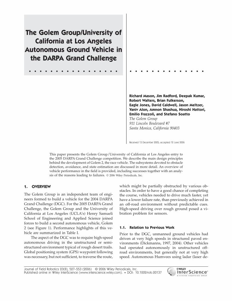
Golem 1, our own first DGC entry, used a singlelaser scanner for obstacle avoidance. Golem 1 trav-eled 5.1 miles in the 2004 Challenge �see Figure 2�,before stopping on a steep slope because of an ex-cessively conservative safety limit on the throttlecontrol. This was the fourth-greatest distance trav-eled in the 2004 DGC; a good performance consider-ing Golem 1’s small total budget of $35,000.

Our attempts to improve on the performance ofprevious researchers were centered on simplifiedstreamlined design—initially in order to conservecosts, but also to enable faster driving by avoidingcomputational bottlenecks. For example, we relied

Figure 1. Golem 2 driving autonomously at 30 miles perhour.

Table I. Golem Group/UCLA performance in the 2005 DARPA Grand Challenge. NQE=National Qualifying Event;GCE=Grand Challenge Event; CMU=Carnegie Mellon University; IVST=Intelligent Vehicle Safety Technologies.

NQE Performance Highlights

9 min 32 s NQE run clearing49/50 gates and 4/4 obstacles

Only Stanford, CMU, and IVST made faster runsclearing all obstacles

Only Stanford and CMU made faster runs clearingat least 49 gates

12 min 19 s NQE run clearing50/50 gates and 5/5 obstacles

Only Stanford, CMU, Princeton, and Cornellmade faster flawless runs

GCE Performance Highlights

Peak speed �controlled driving� 47 mphCompleted 22 race miles in 59 min 28 sAnecdotally said to be fastest vehicle reaching 16-mile DARPA checkpointCrash after 22 miles due to memory management failure

Figure 2. Golem 1 negotiating a gated crossing in the2004 DARPA Grand Challenge. �Photos courtesy ofDARPA.�

528 • Journal of Field Robotics—2006

Journal of Field Robotics DOI 10.1002/rob

primarily on ladar for obstacle avoidance, but unlikethe majority of ladar users, we did not attempt tobuild a three-dimensional �3D� model of the worldper se. Instead, we only attempted to detect the mostimportant terrain features and track the locations ofthose on a two-dimensional �2D� map. Golem 1,with its single ladar scanner, may have gone too farin the direction of simplicity, and Golem 2 carriedmultiple ladars to better distinguish slopes and hill-sides. Ladar obstacle detection is further discussedin Section 3.

As another example of simplification, our pathplanning process considers possible trajectories ofthe truck as simple smooth curves in the 2D plane,with curvature of the trajectory as a measure of driv-ability, and distance to the curve as a proxy for dan-ger of collision. We do not consider obstacles in aconfiguration space of three dimensions, much lesssix dimensions. Our approach might be inadequatefor navigating a wholly general mazelike environ-ment, but more importantly, for our purposes, itgives fast results in the semistructured case of a par-tially obstructed dirt road. Trajectory planning is dis-cussed further in Section 4.

We did experiment with some vision systems inaddition to ladar. Mobileye Vision Technologies, Ltd.provided Golem 2 with a monocular roadfindingsystem, which is discussed in Section 6.1 and also inAlon, Ferencz & Shashua �2006�. This could be con-sidered as extending the cue-based paved-environment work of Dickmanns, and of Mobileye,to an unpaved environment. Experiments with aToshiba stereo vision system are described in Section6.2.

2. VEHICLE DESIGN

Each of our vehicles was a commercially availablepickup truck, fitted with electrically actuated steeringand throttle, and pneumatically actuated brakes.

We felt it was very important that the robot re-mained fully functional as a human-drivable vehicle.Golem 1 seats two people while Golem 2 seats up tofive. A passenger operated the computer and was re-sponsible for testing, while the driver was respon-sible for keeping the vehicle under control and stay-ing aware of the environment. During testing, it wasvery convenient to fluidly transition back and forthbetween autonomous and human control. Individualactuators �brake, accelerator, and steering� can be en-

abled and disabled independently, allowing isolationof a specific problem. Having a human “safetydriver” increased the range of testing scenarios thatwe were willing to consider. Finally, having a street-legal vehicle greatly simplified the logistics.

Accordingly, a central principle behind actuationwas to leave the original controls intact, to as great anextent as possible, in order to keep the vehicle streetlegal. The steering servo had a clutch, which was en-gaged by a pushrod that could be reached from thedriver’s seat. The brakes were actuated by a pneu-matic cylinder that pulled on a cable attached—through the firewall—to the back of the brake pedal.The cable was flexible enough to allow the driver toapply the brakes at any time. The pressure in the cyl-inder could be continuously controlled via a voltage-controlled regulator. A servo was attached directly tothe steering column.

A second design aim was to keep the computa-tional architecture as simple as possible. The coretasks of autonomous driving do not require a largeamount of computational power. We worked to keepthe software running on a single laptop computer.Unburdened by a rack full of computers, we wereable to retain working space in the vehicle, but moreimportantly, any team member could plug in theirlaptop with a universal serial bus �USB� cable and runthe vehicle. A block diagram of the architecture isshown in Figure 3.

2.1. Sensors

The sensors mounted on Golem 2 for vehicle stateestimation included a Novatel ProPak LB-Plus dif-ferential GPS receiver with nominal 14-cm accuracyusing OmniStar HP correction; a BEI C-MIGITS in-ertial measurement unit �IMU�; a custom Hall en-coder on the differential for odometry with approxi-mately 10-cm accuracy; and a 12-bit encoder formeasuring the steering angle. Vehicle state estima-tion is discussed further in Section 5.

The sensors used for terrain perception includeda Sick LMS-221 ladar, which swept a 180° arc in frontof the vehicle—measuring ranges up to 80 m at 361samples/sweep, 37.5 sweeps/s, with the samples in-terleaved 0.5° apart. There were also four Sick LMS-291 ladars, similar in most respects except that theyeach swept a 90° arc while collecting 181 samples/sweep, 75 sweeps/s. The arrangement and functionof the ladars is further discussed in Section 3. A mo-nocular camera system from Mobileye, used for road

Mason et al.: The Golem Group/UCLA in the DARPA Grand Challenge • 529


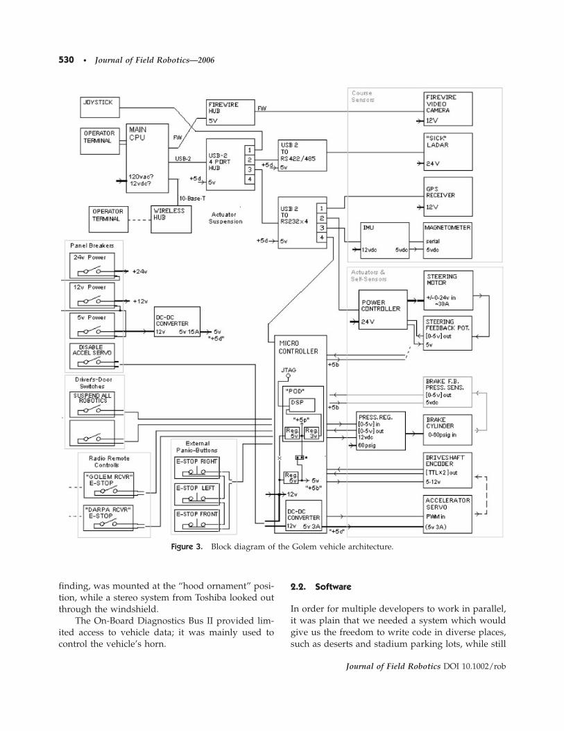
finding, was mounted at the “hood ornament” posi-tion, while a stereo system from Toshiba looked outthrough the windshield.

The On-Board Diagnostics Bus II provided lim-ited access to vehicle data; it was mainly used tocontrol the vehicle’s horn.

2.2. Software

In order for multiple developers to work in parallel,it was plain that we needed a system which wouldgive us the freedom to write code in diverse places,such as deserts and stadium parking lots, while still

Figure 3. Block diagram of the Golem vehicle architecture.



maintaining all features of a revision control system.We found this in the peer-to-peer revision controlsystem, darcs �Roundy, 2005�, which maintains re-positories containing both the source code and acomplete history of changes, and allows a developerto push or pull individual patches from one sourcerepository to another. Using darcs, we achieved avery tight development-test cycle despite our di-verse working environments.

The software ran on a Linux laptop and was di-vided into two main applications. The programwhich made decisions based on sensor input, con-trolled the actuators, and recorded events is knownas golem. It had no connection to the visualizationsoftware dashboard, other than through the logfiles it created, which were human-readable plaintext. Besides being written to disk, these log filescould be piped directly from golem to dashboard,for realtime visualization or replayed offline bydashboard at a later time.

Commands could be typed directly to golem atthe console or received from dashboard over a userdatagram protocol �UDP� port. The commands weredesigned to be simple and easily typed while driv-ing in a moving vehicle on a dirt road. While thiswas convenient, it might have been even more con-venient to be able to use an analog control, or at leastthe arrow keys, to adjust control parameters in realtime.

2.2.1. Golem

The main software for data capture, planning, andcontrol, golem consisted of two threads. The mainthread was completely reactionary and expected tobe real time; it took in data from the sensors, pro-cessed them immediately, and sent commands to theactuators. The low-level drivers, the state estimators,ladar and obstacle filters, the road/path follower, thevelocity profiler, and the controllers all ran in thisthread. A second planning thread was allowed totake more time to come up with globally sensiblepaths for the vehicle, based on snapshots of the ac-cumulated sensor data received at the time thethread was initiated.

Golem could be driven by real-time sensor data,by a simple simulator, or from previously recordedlog data. The simulator was invaluable for debug-ging the high-level behaviors of the planner, but itsmodels were not accurate enough to tune the low-level controllers. The replay mode allowed us to de-

bug the ladar obstacle filters and the state estimatorsin a repeatable way, without having to drive the ve-hicle over and over.

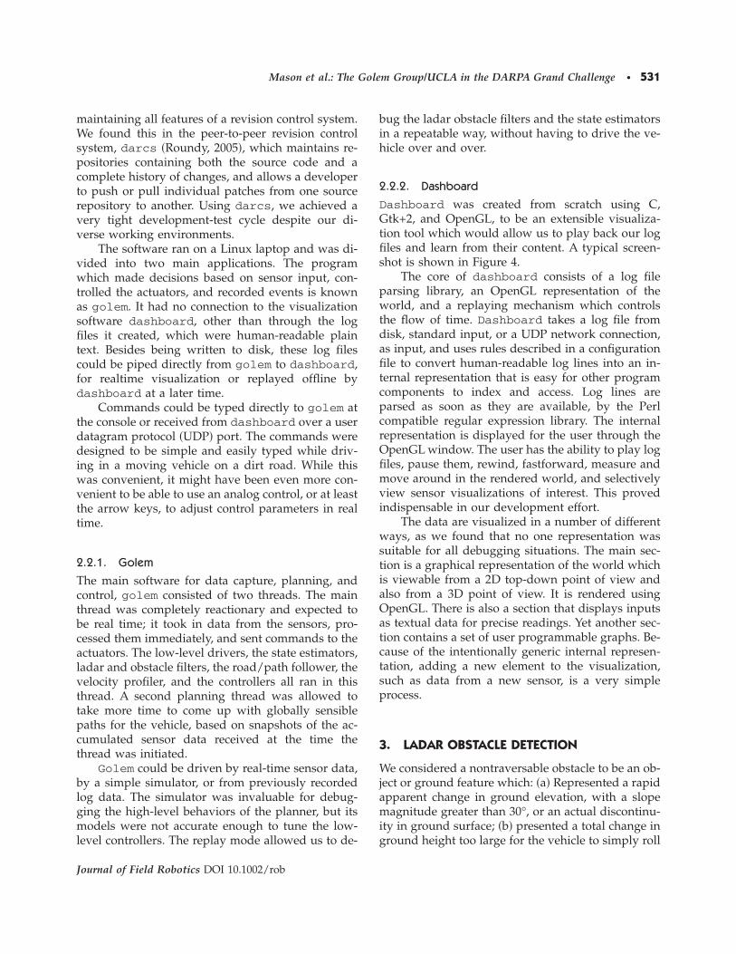
2.2.2. Dashboard

Dashboard was created from scratch using C,Gtk+2, and OpenGL, to be an extensible visualiza-tion tool which would allow us to play back our logfiles and learn from their content. A typical screen-shot is shown in Figure 4.

The core of dashboard consists of a log fileparsing library, an OpenGL representation of theworld, and a replaying mechanism which controlsthe flow of time. Dashboard takes a log file fromdisk, standard input, or a UDP network connection,as input, and uses rules described in a configurationfile to convert human-readable log lines into an in-ternal representation that is easy for other programcomponents to index and access. Log lines areparsed as soon as they are available, by the Perlcompatible regular expression library. The internalrepresentation is displayed for the user through theOpenGL window. The user has the ability to play logfiles, pause them, rewind, fastforward, measure andmove around in the rendered world, and selectivelyview sensor visualizations of interest. This provedindispensable in our development effort.

The data are visualized in a number of differentways, as we found that no one representation wassuitable for all debugging situations. The main sec-tion is a graphical representation of the world whichis viewable from a 2D top-down point of view andalso from a 3D point of view. It is rendered usingOpenGL. There is also a section that displays inputsas textual data for precise readings. Yet another sec-tion contains a set of user programmable graphs. Be-cause of the intentionally generic internal represen-tation, adding a new element to the visualization,such as data from a new sensor, is a very simpleprocess.

3. LADAR OBSTACLE DETECTION

We considered a nontraversable obstacle to be an ob-ject or ground feature which: �a� Represented a rapidapparent change in ground elevation, with a slopemagnitude greater than 30°, or an actual discontinu-ity in ground surface; �b� presented a total change inground height too large for the vehicle to simply roll



over; and �c�, if discontinuous with the ground, wasnot high enough for the vehicle to pass under. Thiswas an adequate definition of an “obstacle” for theDARPA Grand Challenge.1 Since obstacles resultfrom changes in ground elevation, the most criticalinformation comes from comparisons of surface mea-surements adjacent in space.

We did not use sensor data integrated over timeto build a map of absolute ground elevation in theworld frame, on the hypothesis that this is unneces-sarily one step removed from the real information ofinterest. Instead, we tried to directly perceive, or in-

fer, from instantaneous sensor data, regions of rapidchange in ground elevation in the body-fixed frame,and then maintain a map of those regions in theworld frame. We did not concern ourselves with anyground slope or surface roughness that did not rise tothe threshold of making the ground nontraversable.

3.1. Ladar Geometry

We used Sick LMS-291 and LMS-221 laser scannersas our primary means of obstacle detection. It is in-teresting that the many DGC teams using 2D ladars,such as these, found a wide variety of ways of ar-ranging them. These ladars sweep a rangefinding la-ser beam through a sector of a plane, while the planeitself can be rotated or translated, either by vehiclemotion or by actuating the ladar mount. The choice

1Ideally, one would like to classify some objects, such as plants, as“soft obstacles” that can be driven over even if they appear tohave steep sides. Other hazards, such as water or marshy ground,cannot be classified simply as changes in ground elevation. Butthis increased level of sophistication was not necessary to com-plete the DGC and remains a topic of future work for us.

Figure 4. Dashboard visualization of Golem 2 entering a tunnel during a NQE run.



of plane or, more generally, the choice of scan pat-tern for any beam-based sensor, represents a choicebetween scanning rapidly in the azimuthal direction,with slower or sparser sampling at different eleva-tion angles, or the reverse.

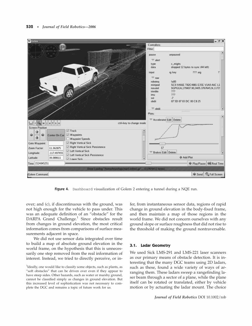
A ladar scanning in the vertical plane has thesignificant advantage that the traversability of thescanned terrain is apparent from a single lasersweep. For example, it is easily determined from thesingle vertical-plane scan in Figure 5 that the groundis continuous, flat, and traversable from a few feetbefore the truck, up to the point where there is anontraversable vertical surface taller than the vehi-cle’s wheels.

In our case, a single-laser sweep takes 1/75 sand individual sample points are separated by1/13,575 s. On this time scale, it is not likely thatmotion or vibration of the vehicle could distort thevertical scan sufficiently to alter this interpretation�make the traversable ground appear nontraversableor vice versa�. Similarly, while small errors in theestimated pitch of the vehicle would induce smallerrors in the estimated location of the nontraversableobstacle, it is not likely that they could cause a majorerror or prevent the perception of an obstacle in theright approximate location. Against these advan-tages is the obvious drawback that a vertical sliceonly measures the terrain in a single-narrow direc-tion. Even if there are multiple vertical scannersand/or the vertical plane can be turned in differentdirections, the vehicle is likely to have a blinkeredview with sparse azimuthal coverage of the terrain,and may miss narrow obstacles.

Conversely, a scan plane which is horizontal, ornearly, horizontal, will provide good azimuthal cov-erage, and clearly show narrow obstacles, such asfenceposts and pedestrians, but the interpretation of

any single-horizontal scan in isolation is problem-atic. Lacking measurements at adjacent elevationangles, one cannot determine if a return from asingle-horizontal scan is from a nontraversable steepsurface or from a traversable gently sloping one.Therefore, the information from multiple horizontalscans must be combined; but since the crucial com-parisons are now between individual measurementstaken at least 1/75 s apart instead of 1/13,575 sapart, there is a greater likelihood that imperfectlyestimated motion or vibration will distort the data.Small errors in pitch, roll, or altitude could cause thevehicle to misapprehend the height of a ground con-tour and lead to a totally erroneous classification ofthe terrain as traversable or nontraversable.

Our approach was to use a complementary ar-rangement of both vertical and nearly horizontal la-dars. On the Golem 2 vehicle, there are two nearlyhorizontal ladars and three vertically oriented ladarsmounted on the front bumper. The idea is that thevertically oriented ladars are used to form a profileof the general ground surface in front of the truck, inthe truck body-fixed frame �as opposed to a world-fixed frame�. The ground model we fit to the datawas piece-wise linear in the truck’s direction of mo-tion, and piece-wise constant in the sideways direc-tion. The model interpolated the most recent avail-able ladar data. In locations beyond the availabledata, the ground was assumed to have constant alti-tude in the body-fixed frame.

The apparent altitude of returns, from the nearlyhorizontal ladars relative to the ground model, wasthen computed to see if those returns were: �a� Con-sistent with a traversable part of the ground model;�b� consistent with a nontraversable part of theground model; �c� apparently from an elevationmoderately higher than the notional ground; or �d�apparently from an object so far above the notionalground that the vehicle should be able to pass underit. In either Case �b� or �c�, the ladar return is classi-fied as arising from a possible obstacle; after severalof these returns are received from the same locationat different vantage points, the presence of an ob-stacle is confirmed. In practice, an object, such as aparked car, will be represented as a cluster of adja-cent obstacles.

For example, Figure 6 illustrates ladar data froma portion of the NQE course. The returns from thehorizontally oriented ladars indicated a long straightfeature crossing in front of the vehicle, and twosmaller features, or clusters, of returns. The three

Figure 5. Returns from a ladar oriented in a verticalplane.



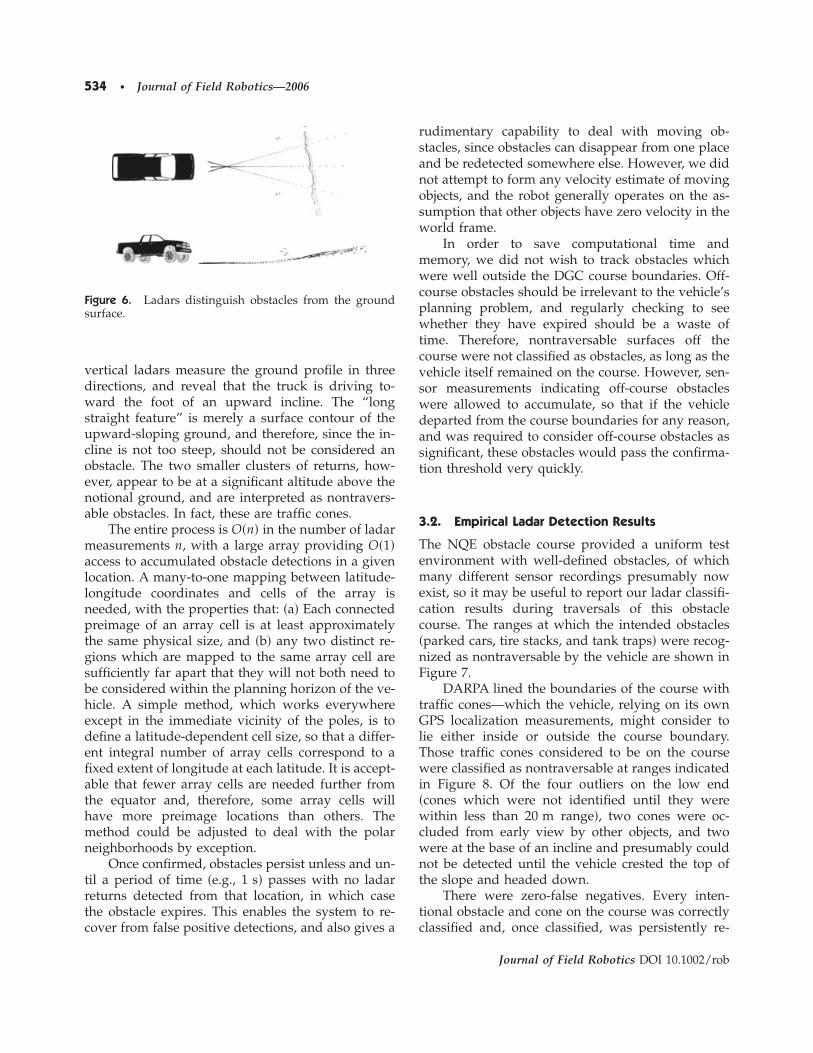
vertical ladars measure the ground profile in threedirections, and reveal that the truck is driving to-ward the foot of an upward incline. The “longstraight feature” is merely a surface contour of theupward-sloping ground, and therefore, since the in-cline is not too steep, should not be considered anobstacle. The two smaller clusters of returns, how-ever, appear to be at a significant altitude above thenotional ground, and are interpreted as nontravers-able obstacles. In fact, these are traffic cones.

The entire process is O�n� in the number of ladarmeasurements n, with a large array providing O�1�access to accumulated obstacle detections in a givenlocation. A many-to-one mapping between latitude-longitude coordinates and cells of the array isneeded, with the properties that: �a� Each connectedpreimage of an array cell is at least approximatelythe same physical size, and �b� any two distinct re-gions which are mapped to the same array cell aresufficiently far apart that they will not both need tobe considered within the planning horizon of the ve-hicle. A simple method, which works everywhereexcept in the immediate vicinity of the poles, is todefine a latitude-dependent cell size, so that a differ-ent integral number of array cells correspond to afixed extent of longitude at each latitude. It is accept-able that fewer array cells are needed further fromthe equator and, therefore, some array cells willhave more preimage locations than others. Themethod could be adjusted to deal with the polarneighborhoods by exception.

Once confirmed, obstacles persist unless and un-til a period of time �e.g., 1 s� passes with no ladarreturns detected from that location, in which casethe obstacle expires. This enables the system to re-cover from false positive detections, and also gives a

rudimentary capability to deal with moving ob-stacles, since obstacles can disappear from one placeand be redetected somewhere else. However, we didnot attempt to form any velocity estimate of movingobjects, and the robot generally operates on the as-sumption that other objects have zero velocity in theworld frame.

In order to save computational time andmemory, we did not wish to track obstacles whichwere well outside the DGC course boundaries. Off-course obstacles should be irrelevant to the vehicle’splanning problem, and regularly checking to seewhether they have expired should be a waste oftime. Therefore, nontraversable surfaces off thecourse were not classified as obstacles, as long as thevehicle itself remained on the course. However, sen-sor measurements indicating off-course obstacleswere allowed to accumulate, so that if the vehicledeparted from the course boundaries for any reason,and was required to consider off-course obstacles assignificant, these obstacles would pass the confirma-tion threshold very quickly.

3.2. Empirical Ladar Detection Results

The NQE obstacle course provided a uniform testenvironment with well-defined obstacles, of whichmany different sensor recordings presumably nowexist, so it may be useful to report our ladar classifi-cation results during traversals of this obstaclecourse. The ranges at which the intended obstacles�parked cars, tire stacks, and tank traps� were recog-nized as nontraversable by the vehicle are shown inFigure 7.

DARPA lined the boundaries of the course withtraffic cones—which the vehicle, relying on its ownGPS localization measurements, might consider tolie either inside or outside the course boundary.Those traffic cones considered to be on the coursewere classified as nontraversable at ranges indicatedin Figure 8. Of the four outliers on the low end�cones which were not identified until they werewithin less than 20 m range�, two cones were oc-cluded from early view by other objects, and twowere at the base of an incline and presumably couldnot be detected until the vehicle crested the top ofthe slope and headed down.

There were zero-false negatives. Every inten-tional obstacle and cone on the course was correctlyclassified and, once classified, was persistently re-

Figure 6. Ladars distinguish obstacles from the groundsurface.



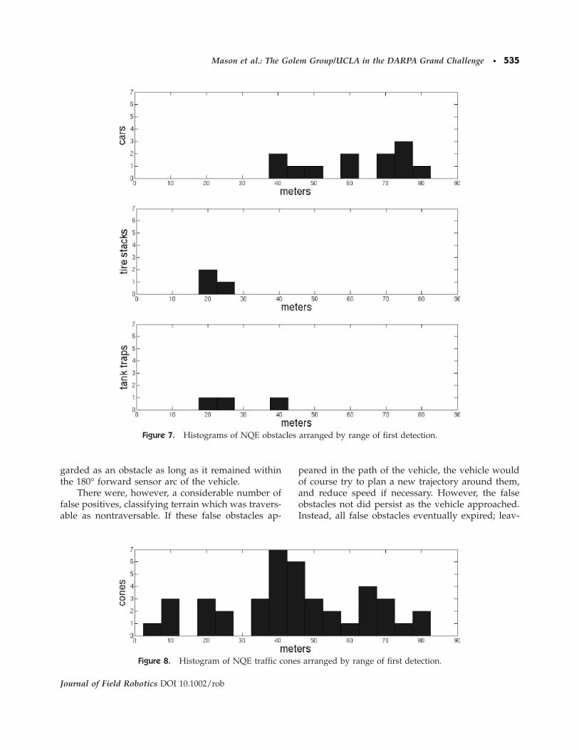
garded as an obstacle as long as it remained withinthe 180° forward sensor arc of the vehicle.

There were, however, a considerable number offalse positives, classifying terrain which was travers-able as nontraversable. If these false obstacles ap-

peared in the path of the vehicle, the vehicle wouldof course try to plan a new trajectory around them,and reduce speed if necessary. However, the falseobstacles not did persist as the vehicle approached.Instead, all false obstacles eventually expired; leav-

Figure 7. Histograms of NQE obstacles arranged by range of first detection.

Figure 8. Histogram of NQE traffic cones arranged by range of first detection.



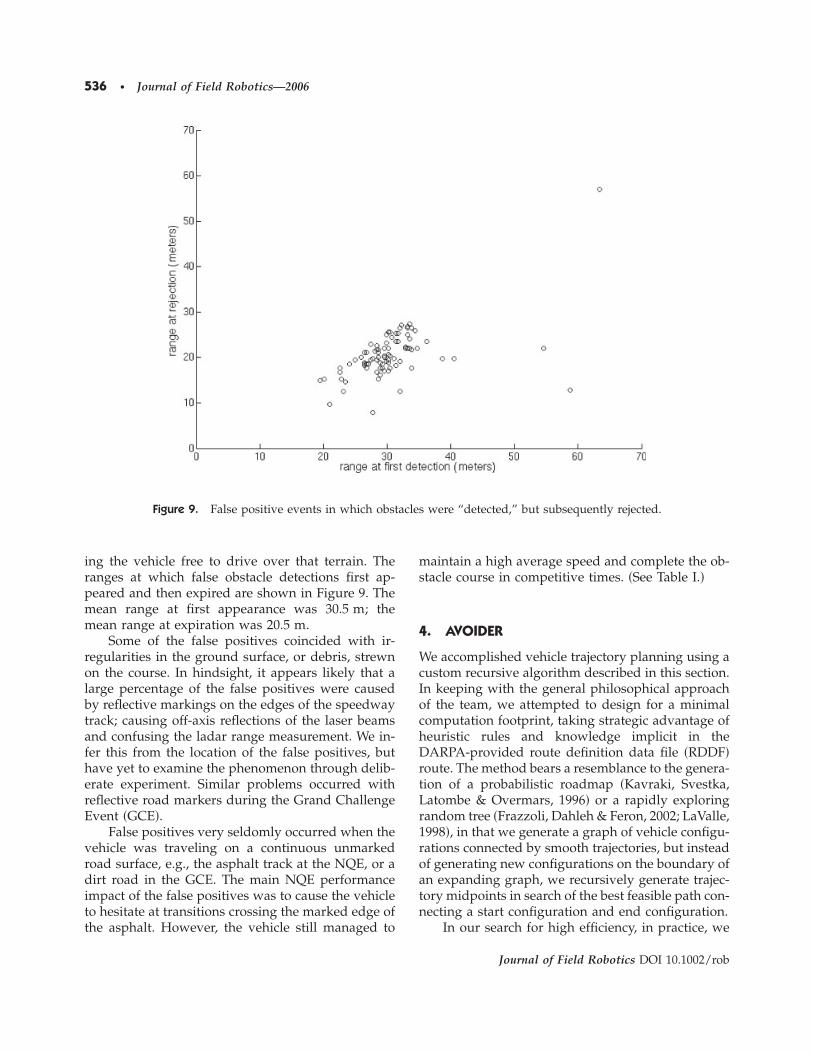
ing the vehicle free to drive over that terrain. Theranges at which false obstacle detections first ap-peared and then expired are shown in Figure 9. Themean range at first appearance was 30.5 m; themean range at expiration was 20.5 m.

Some of the false positives coincided with ir-regularities in the ground surface, or debris, strewnon the course. In hindsight, it appears likely that alarge percentage of the false positives were causedby reflective markings on the edges of the speedwaytrack; causing off-axis reflections of the laser beamsand confusing the ladar range measurement. We in-fer this from the location of the false positives, buthave yet to examine the phenomenon through delib-erate experiment. Similar problems occurred withreflective road markers during the Grand ChallengeEvent �GCE�.

False positives very seldomly occurred when thevehicle was traveling on a continuous unmarkedroad surface, e.g., the asphalt track at the NQE, or adirt road in the GCE. The main NQE performanceimpact of the false positives was to cause the vehicleto hesitate at transitions crossing the marked edge ofthe asphalt. However, the vehicle still managed to

maintain a high average speed and complete the ob-stacle course in competitive times. �See Table I.�

4. AVOIDER

We accomplished vehicle trajectory planning using acustom recursive algorithm described in this section.In keeping with the general philosophical approachof the team, we attempted to design for a minimalcomputation footprint, taking strategic advantage ofheuristic rules and knowledge implicit in theDARPA-provided route definition data file �RDDF�route. The method bears a resemblance to the genera-tion of a probabilistic roadmap �Kavraki, Svestka,Latombe & Overmars, 1996� or a rapidly exploringrandom tree �Frazzoli, Dahleh & Feron, 2002; LaValle,1998�, in that we generate a graph of vehicle configu-rations connected by smooth trajectories, but insteadof generating new configurations on the boundary ofan expanding graph, we recursively generate trajec-tory midpoints in search of the best feasible path con-necting a start configuration and end configuration.

In our search for high efficiency, in practice, we

Figure 9. False positive events in which obstacles were “detected,” but subsequently rejected.



forfeited any guarantee of the global optimality ofour solution paths and even predictable convergenceconditions for the routine. However, we found that inthe vast majority of cases, traversable paths are rap-idly found without burdening the processing re-sources of the vehicle.

The stage for the planning algorithm is a Carte-sian 2D map in the vicinity of the initial global coor-dinates of the vehicle, populated with a number ofdiscrete obstacles. The obstacles are represented aspoint hazards that must be avoided by a particularradius, or as line segments that can be crossed in onlyone direction. Point obstacles are centered on loca-tions in the plane that have been identified as non-traversable by the ladar system. The buffer radiussurrounding each point obstacle includes the physi-cal width of the vehicle and, additionally, variesbased on the distance from the vehicle to the hazard.A real object, such as a wall or car, is represented bya cluster of such points, each with its associated ra-dius. Line segment obstacles arise from the RDDF,which specifies corridor boundaries for the vehicle.The vehicle trajectory is a single curve describing themotion of the vehicle frame in the plane.

Our task is to find a drivable path from an initialconfiguration to a destination configuration that doesnot encroach on any obstacle.2 The destination istaken to be the center of the RDDF corridor at somedistance ahead of our sensor horizon. The simplestand presumably most frequently occurring scenariowill require the vehicle to simply drive forwardfrom/to without performing any evasive maneuvers.We represent this scenario with a directed acyclicgraph containing two nodes and a single connectingedge. This choice of data structure later allows us totake advantage of a topographically sorted ordering,that enables the least cost traversal of the graph to befound in linear time �O�N edges��. Each node in thegraph is associated with a possible configuration ofthe vehicle, and each edge is associated with a di-rected path connecting a starting configuration to atarget configuration. At all times, care is taken tomaintain the topological correspondence between thenodes in the graph and the locations in the local map.

After initialization we enter the recursive loop ofthe algorithm, which consists of three stages:

1. Graph Evaluation,

2. Path Validation, and3. Graph Expansion.

This loop is executed repeatedly until a satisfac-tory path is found from/to, or until a watchdog ter-mination condition is met. Typically, we would ter-minate the planner if a path was not found afterseveral hundred milliseconds.

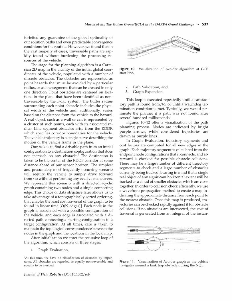
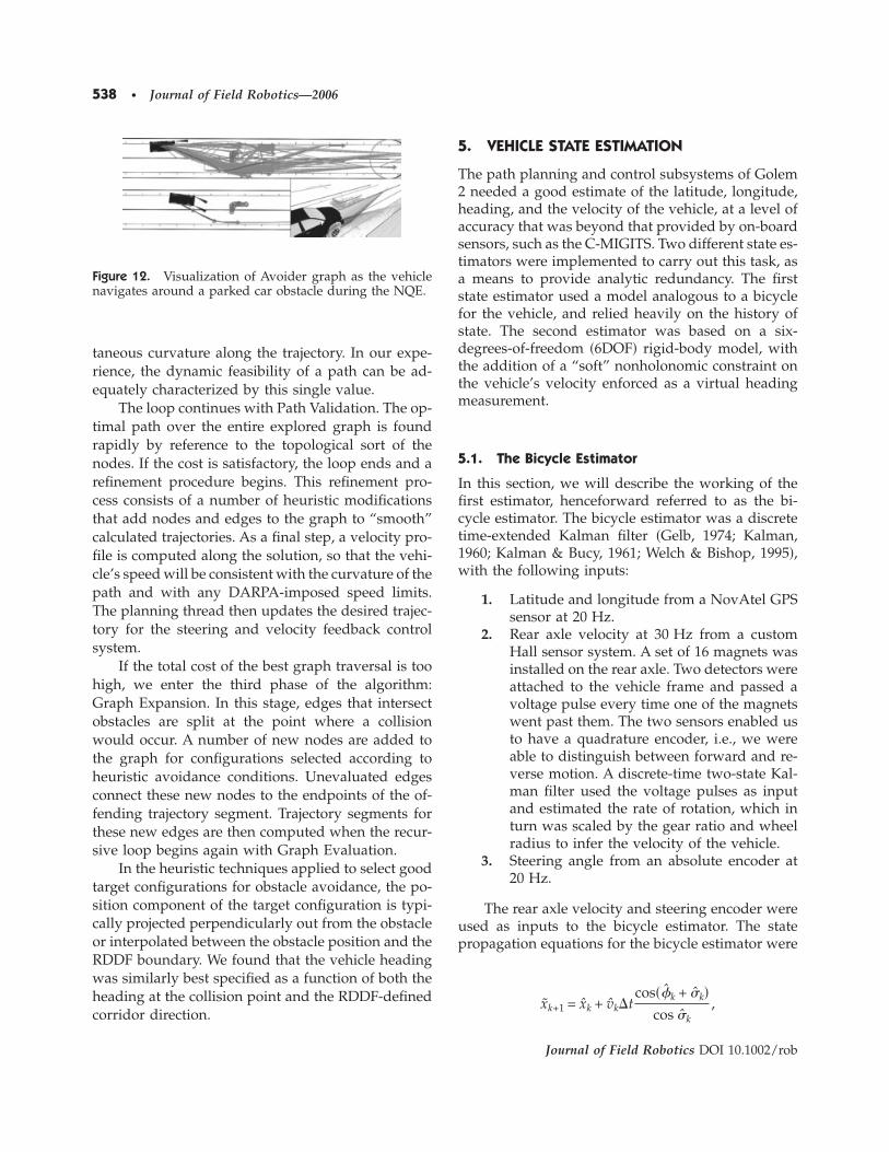
Figures 10–12 offer a visualization of the pathplanning process. Nodes are indicated by brightpurple arrows, while considered trajectories aredrawn as purple lines.

In Graph Evaluation, trajectory segments andcost factors are computed for all new edges in thegraph. Each trajectory segment is calculated from theendpoint node configurations that it connects, and af-terward is checked for possible obstacle collisions.There may be a large number of different trajectorysegments to check and a large number of obstaclescurrently being tracked, bearing in mind that a singlereal object of any significant horizontal extent will betracked as a cloud of smaller obstacles which are closetogether. In order to collision check efficiently, we usea wavefront propagation method to create a map in-dicating the approximate distance from each point tothe nearest obstacle. Once this map is produced, tra-jectories can be checked rapidly against it for obstaclecollisions. If no obstacles are intersected, the cost oftraversal is generated from an integral of the instan-

2At this time, we have no classification of obstacles by impor-tance. All obstacles are regarded as equally nontraversable andequally to be avoided.

Figure 11. Visualization of Avoider graph as the vehiclenavigates around a tank trap obstacle during the NQE.

Figure 10. Visualization of Avoider algorithm at GCEstart line.



taneous curvature along the trajectory. In our expe-rience, the dynamic feasibility of a path can be ad-equately characterized by this single value.

The loop continues with Path Validation. The op-timal path over the entire explored graph is foundrapidly by reference to the topological sort of thenodes. If the cost is satisfactory, the loop ends and arefinement procedure begins. This refinement pro-cess consists of a number of heuristic modificationsthat add nodes and edges to the graph to “smooth”calculated trajectories. As a final step, a velocity pro-file is computed along the solution, so that the vehi-cle’s speed will be consistent with the curvature of thepath and with any DARPA-imposed speed limits.The planning thread then updates the desired trajec-tory for the steering and velocity feedback controlsystem.

If the total cost of the best graph traversal is toohigh, we enter the third phase of the algorithm:Graph Expansion. In this stage, edges that intersectobstacles are split at the point where a collisionwould occur. A number of new nodes are added tothe graph for configurations selected according toheuristic avoidance conditions. Unevaluated edgesconnect these new nodes to the endpoints of the of-fending trajectory segment. Trajectory segments forthese new edges are then computed when the recur-sive loop begins again with Graph Evaluation.

In the heuristic techniques applied to select goodtarget configurations for obstacle avoidance, the po-sition component of the target configuration is typi-cally projected perpendicularly out from the obstacleor interpolated between the obstacle position and theRDDF boundary. We found that the vehicle headingwas similarly best specified as a function of both theheading at the collision point and the RDDF-definedcorridor direction.

5. VEHICLE STATE ESTIMATION

The path planning and control subsystems of Golem2 needed a good estimate of the latitude, longitude,heading, and the velocity of the vehicle, at a level ofaccuracy that was beyond that provided by on-boardsensors, such as the C-MIGITS. Two different state es-timators were implemented to carry out this task, asa means to provide analytic redundancy. The firststate estimator used a model analogous to a bicyclefor the vehicle, and relied heavily on the history ofstate. The second estimator was based on a six-degrees-of-freedom �6DOF� rigid-body model, withthe addition of a “soft” nonholonomic constraint onthe vehicle’s velocity enforced as a virtual headingmeasurement.

5.1. The Bicycle Estimator

In this section, we will describe the working of thefirst estimator, henceforward referred to as the bi-cycle estimator. The bicycle estimator was a discretetime-extended Kalman filter �Gelb, 1974; Kalman,1960; Kalman & Bucy, 1961; Welch & Bishop, 1995�,with the following inputs:

1. Latitude and longitude from a NovAtel GPSsensor at 20 Hz.

2. Rear axle velocity at 30 Hz from a customHall sensor system. A set of 16 magnets wasinstalled on the rear axle. Two detectors wereattached to the vehicle frame and passed avoltage pulse every time one of the magnetswent past them. The two sensors enabled usto have a quadrature encoder, i.e., we wereable to distinguish between forward and re-verse motion. A discrete-time two-state Kal-man filter used the voltage pulses as inputand estimated the rate of rotation, which inturn was scaled by the gear ratio and wheelradius to infer the velocity of the vehicle.

3. Steering angle from an absolute encoder at20 Hz.

The rear axle velocity and steering encoder wereused as inputs to the bicycle estimator. The statepropagation equations for the bicycle estimator were

xk+1 = xk + vk�tcos��k + �k�

cos �k,

Figure 12. Visualization of Avoider graph as the vehiclenavigates around a parked car obstacle during the NQE.



yk+1 = yk + vk�tsin��k + �k�

cos �k,

�k+1 = �k +vk�t

dtan �k, �1�

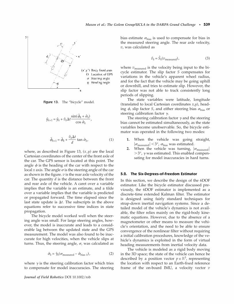
where, as described in Figure 13, �x ,y� are the localCartesian coordinates of the center of the front axle ofthe car. The GPS sensor is located at this point. Theangle � is the heading of the car with respect to thelocal x axis. The angle � is the steering angle of the caras shown in the figure. v is the rear axle velocity of thecar. The quantity d is the distance between the frontand rear axle of the vehicle. A caret over a variableimplies that the variable is an estimate, and a tildeover a variable implies that the variable is predictedor propagated forward. The time elapsed since thelast state update is �t. The subscripts in the aboveequations refer to successive time indices in statepropagation.

The bicycle model worked well when the steer-ing angle was small. For large steering angles, how-ever, the model is inaccurate and leads to a consid-erable lag between the updated state and the GPSmeasurement. The model was also found to be inac-curate for high velocities, when the vehicle slips atturns. Thus, the steering angle, �, was calculated as

�k = �k��measured − �bias k� , �2�

where � is the steering calibration factor which triesto compensate for model inaccuracies. The steering

bias estimate �bias is used to compensate for bias inthe measured steering angle. The rear axle velocity,v, was calculated as

vk = Sk�vmeasured� , �3�

where vmeasured is the velocity being input to the bi-cycle estimator. The slip factor S compensates forvariations in the vehicle’s apparent wheel radius,and for the fact that the vehicle may be going uphillor downhill, and tries to estimate slip. However, theslip factor was not able to track consistently longperiods of slipping.

The state variables were latitude, longitude�translated to local Cartesian coordinates x,y�, head-ing �, slip factor S, and either steering bias �bias orsteering calibration factor �.

The steering calibration factor � and the steeringbias cannot be estimated simultaneously, as the statevariables become unobservable. So, the bicycle esti-mator was operated in the following two modes:

1. When the vehicle was going straight,��measured � �3°, �bias was estimated.

2. When the vehicle was turning, ��measured ��3°, � was estimated. This enabled compen-sating for model inaccuracies in hard turns.

5.2. The Six-Degrees-of-Freedom Estimator

In this section, we describe the design of the 6DOFestimator. Like the bicycle estimator discussed pre-viously, the 6DOF estimator is implemented as adiscrete-time extended Kalman filter. The estimatoris designed using fairly standard techniques forstrap-down inertial navigation systems. Since a de-tailed model of the vehicle’s dynamics is not avail-able, the filter relies mainly on the rigid-body kine-matic equations. However, due to the absence of amagnetometer or other means to measure the vehi-cle’s orientation, and the need to be able to ensureconvergence of the nonlinear filter without requiringa initial calibration procedures, knowledge of the ve-hicle’s dynamics is exploited in the form of virtualheading measurements from inertial velocity data.

The vehicle is modeled as a rigid body movingin the 3D space; the state of the vehicle can hence bedescribed by a position vector p�R3, representingthe location with respect to an Earth-fixed referenceframe of the on-board IMU, a velocity vector v

Figure 13. The “bicycle” model.



=dp/dt, and a rotation matrix R�SO�3�, whereSO�3� is known as the Special Orthogonal group inthe 3D space, and includes all orthogonal 3�3 ma-trices with a determinant equal to +1. The columnsof R can be thought of as expressing the coordinatesof an orthogonal triad rigidly attached to the vehi-cle’s body �body axes�.

The inputs to the estimator are the accelerationand angular rate measurements from the IMU, pro-vided at 100 Hz, and the GPS data, provided atabout 20 Hz. In addition, the estimator has access tothe velocity data from the Hall sensors mounted onthe wheels, and to the steering angle measurement.

In the following, we will indicate the accelera-tion measurements with za�R3, and the angular ratemeasurements with zg�R3. Moreover, we use Za toindicate the unique skew-symmetric matrix, suchthat Zav=za�v, for all v�R3. A similar conventionwill be used for zg and other 3D vectors throughoutthis section.

The IMU accelerometers measure the vehicle’sinertial acceleration, measured in body-fixed coordi-nates, minus the gravity acceleration; in otherwords,

za = RT�a − g� + na,

where a and g are, respectively, the vehicle’s accel-eration, and gravity acceleration in the inertialframe, and na is an additive, white Gaussian mea-surement noise. Since the C-MIGITS IMU estimatesaccelerometer biases, and outputs corrected mea-surements, we consider na as a zero-mean noise.

The IMU solid-state rate sensors measure the ve-hicle’s angular velocity, in body axes. In otherwords,

zg = � + ng,

where � is the vehicle’s angular velocity �in bodyaxes�, and ng is an additive, white Gaussian mea-surement noise. As in the case of acceleration mea-surements, ng is assumed to be unbiased.

The kinematics of the vehicle are described bythe equations

p = v ,

v = a ,

R = R , �4�

where is the skew-symmetric matrix correspond-ing to the angular velocity �, and we ignored the Co-riolis terms for simplicity. As a matter of fact, this isjustified in our application due to the low speed, rela-tively short range, and to the fact that errors inducedby vibrations and irregularities in the terrain aredominant with respect to the errors induced by ignor-ing the Coriolis acceleration terms.

We propagate the estimate of the state of the ve-hicle using the following continuous-time model, inwhich the hat indicates estimates:

p = v ,

v = Rza + g ,

R˙

= RZg. �5�

An exact time discretization of the above, under theassumption that the �inertial� acceleration and angu-lar velocity are constant during the sampling time, is

p+ = p + v�t + 12 �Rza + g��t2,

v+ = v + �Rza + g��t ,

R+ = R exp�Zg�t� . �6�

The matrix exponential appearing in the attitudepropagation equation can be computed using Rod-rigues’ formula. Given a skew-symmetric 3�3 ma-trix M, write it as the product M=, such that isthe skew-symmetric matrix corresponding to a unitvector �; then

exp�M� = exp�� = I + sin + 2�1 − cos � .

�7�

The error in the state estimate is modeled as anine-dimensional vector �x= ��p ,�v ,��, where



p = p + �p ,

v = v + �v ,

R = R exp�� . �8�

Note that the components of the vector �� can be un-derstood as the elementary rotation angles about thebody-fixed axes that make R coincide with R; such arotation, representing the attitude error, can also bewritten as �R=exp��= RTR.

The linearized error dynamics are written asfollows:

ddt

�x = A�x + Fn , �9�

where

A ª �0 I 0

0 0 − RZa

0 0 − Zg�, F ª �0 0

R 0

0 I� . �10�

When no GPS information is available, the estima-tion error covariance matrix PªE��x��x�T� is propa-gated through numerical integration of the ordinarydifferential equation

ddt

P = AP + PAT + FQFT.

Position data from the GPS are used to updatethe error covariance matrix and the state estimate.The measurement equation is simply zGPS=p+nGPS.In order to avoid numerical instability, we use theUD-factorization method described in Rogers �2003�to update the error covariance matrix and to com-pute the filter gain K.

Since the vehicle’s heading is not observablesolely from GPS data, and we wished to reduce thecalibration and initialization procedures to a mini-mum �e.g., to allow for seamless resets of the filterduring the race�, we impose a soft constraint on theheading through a virtual measurement of the iner-tial velocity, of the form

zNHC = arctan� vEast

vNorth − � ,

where � is the measured steering angle, and is afactor accounting for the fact that the origin of thebody reference frame is not on the steering axle.

In other words, we effectively impose a non-holonomic constraint �NHC� on the motion of thevehicle through a limited-sideslip assumption. Thisassumption is usually satisfied when the vehicle istraveling straight, but may not be satisfied duringturns. Moreover, when the vehicle is moving veryslowly, the direction of the velocity is difficult to es-timate, as the magnitude of the velocity vector isdominated by the estimation error. Hence, the vir-tual measurement is applied only when the steeringangle is less than 10°, and the vehicle’s speed is atleast 2.5 mph �both values were determinedempirically�.

The filter described in this section performedsatisfactorily in our tests and during the DGC race,providing the on-board control algorithms with po-sition and heading estimates that were nominallywithin 10 cm and 0.1°, respectively.

5.3. Modeling System Noise

The state was propagated and updated every time aGPS signal arrived. There was no noise associatedwith the state propagation equation �1�. It was as-sumed that there was additive white Gaussian noiseassociated with the inputs �vmeasured and �measured forthe bicycle model, and za and zg for the six-degrees-of-freedom model�. To efficiently track the constantsin the state variables �S, �bias, ��, it was assumed thatthere was an additive white Gaussian noise term intheir propagation. It was also assumed that the GPSmeasurement �latitude and longitude� had somenoise associated with it. The variances assigned tothe noise processes described above were tuned toensure that the innovations3 were uncorrelated, andthat the estimator was stable, and converged reason-ably quickly. By tuning the variances, we can alterthe “trust” associated with the history of the vehiclestate or with the GPS measurement.

3Innovation of a measured data is the difference between the es-timated and the measured data.



5.3.1. Determining the Appropriate GPSMeasurement Noise Variance

The received data from the GPS consisted of the lati-tude, longitude, and a horizontal dilution of preci-sion �HDOP� value. HDOP is a figure of merit forthe GPS measurement, which is directly related tothe number of satellites visible to the GPS antenna.The HDOP value is related to the noise in each mea-surement. However, our attempts at mapping theHDOP values to actual variances were futile, as wedid not observe a monotonic relationship. It was no-ticed that an HDOP of more than 5 usually corre-sponded to multipath reception in GPS, and conse-quently, the GPS had an abnormally huge variancein that case. In the absence of any ad hoc relationshipbetween the HDOP and noise variance, we opted tokeep a constant variance associated with GPS noiseif the HDOP was less than 5 and a huge varianceotherwise. Also, we noticed that the GPS noise washighly correlated and not white.

5.3.2. Projection of the Innovations

The bicycle estimator is based on a very intuitivemodel of the vehicle, which motivates us to considerthe GPS innovations in a physically relevant refer-ence frame, rather than any arbitrary referenceframe. It is insightful to project the innovations intothe local frame of the vehicle: Parallel to the headingdirection and perpendicular to it. The parallel andperpendicular body fixed axes are indicated in Fig-ure 13.

For an ideal estimator, the innovations will beuncorrelated with each other. However, we tunedthe estimator to just achieve innovations with zeromean. While tuning the estimator, it was very usefulto consider the parallel and perpendicular innova-tions. For example, a direct current bias in the paral-lel innovations implied that we were not trackingthe slip factor �S� adequately. Thus, to ensure a zero-mean parallel innovation, the variance associatedwith the propagation of slip factor should beincreased.

5.3.3. Adaptive Shaping of the Innovations

The noise in the GPS data was highly correlated, andthere was very little a priori knowledge of the vari-ance. Very often, especially when the vehicle woulddrive near a wall or approach a tunnel, there wouldbe highly erratic jumps in the GPS measurements

due to multipath reflections. Without any a prioriknowledge of the variance in such cases, the stateestimate would bounce around a lot. This was unde-sirable as it would hamper the path planner and theobstacle detection subroutines in the main program.

To counter these “unphysical” jumps, once theestimator was converged, the innovations wereclipped up to a certain maximum absolute value. Forexample, a GPS measurement corresponding to aperpendicular innovation of 2 m in 0.05 s while go-ing straight is unphysical, and so perpendicular in-novation should be clipped to a nominal value �inour case, 6 in.�. This prevented large jumps in stateestimate, but had a grave disadvantage. It was ob-served that if the innovations were clipped to a fixedrange, then in certain situations, the state estimatewill lag far behind from a “good” set of GPS mea-surements, and take a long time to converge back. Toprevent this from happening, the clipping limit ofthe innovations was determined adaptively as theminimum of either a fixed limit, or the mean of theinnovations in the last 2 s scaled by a numerical fac-tor slightly greater than unity. The parallel and per-pendicular components of the innovation wereclipped separately with different numerical con-stants used.

5.3.4. Countering the Time Delays

There was some finite delay between the appearanceof sensor data on the bus and the time they wereprocessed by the control program. Usually, this de-lay was nominal �50–200 �s�, but it was sporadi-cally very large. A large delay in GPS data mani-fested in large negative parallel innovation.However, the large innovation was clipped effec-tively by the method described earlier, and conse-quently did not effect the state estimate. In the fu-ture, we plan to implement a routine whichsynchronizes the time between all the serial/USBdata sources.

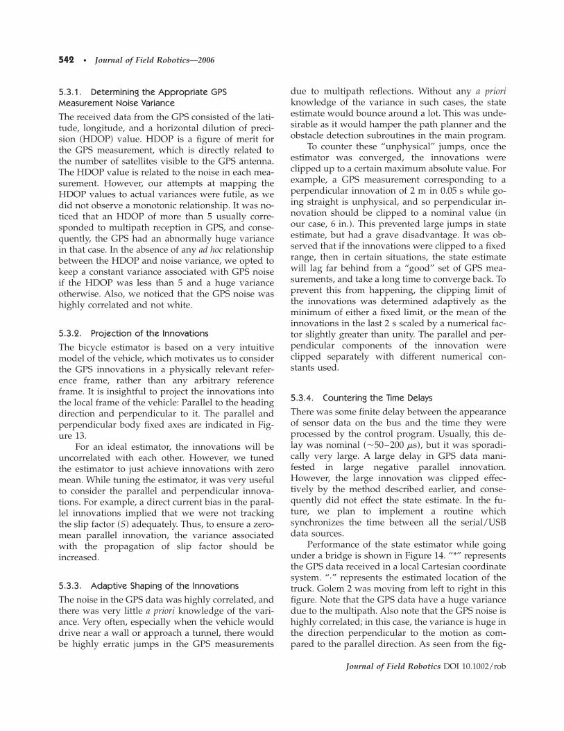
Performance of the state estimator while goingunder a bridge is shown in Figure 14. “*” representsthe GPS data received in a local Cartesian coordinatesystem. “·” represents the estimated location of thetruck. Golem 2 was moving from left to right in thisfigure. Note that the GPS data have a huge variancedue to the multipath. Also note that the GPS noise ishighly correlated; in this case, the variance is huge inthe direction perpendicular to the motion as com-pared to the parallel direction. As seen from the fig-



ure, the performance of the state estimator is im-mune to the large unphysical jumps in GPS data.Occasional jumps of length 0.3 m are observed inthe successive updates of estimated state. These cor-respond to a delay in received GPS data and largenegative parallel innovations, as discussed in thissection.

5.3.5. Special Modes of Operation

There were a couple of situations that required spe-cial handling instructions:

• The GPS signal was observed to drift consid-erably when the vehicle was at rest. Not onlywas this unphysical, but it is also detrimentalto path planning. Thus, when the vehicle wasgoing considerably slowly or was at rest, thevariance assigned to the GPS measurementswas increased significantly. In such a case, thebicycle estimator essentially worked as an in-tegrator, rather than a filter.

• It was observed that the GPS signal wouldoccasionally jump discretely. These jumpsusually corresponded to the presence of apower transmission line nearby. The diffi-culty was that the GPS took a while ��2 s� toreconverge after the jumps. These unphysicaljumps were easily detected from the jumps inthe parallel and perpendicular innovations.

After the detection of such jumps, the GPSvariance was increased until it was trustwor-thy again, i.e., until the innovations werewithin a certain limit again.

5.3.6. Initialization of the IMU

One advantage of this model was that it convergedvery fast while going straight, usually in approxi-mately 5 s. Once the bicycle model converged, theheading estimate was used to initialize the IMU.While going straight, the performance of the bicycleestimator was extremely good as the heading esti-mate was within 0.5° of the IMU-computed heading.However, on sharp turns, the heading estimate wasup to 3° from the IMU-computed heading. Thus,the IMU-computed heading was given more impor-tance, especially when GPS signals were bad. In thefuture, we plan to extend the bicycle model to in-clude the angular rotation and linear displacementdata from the IMU.

6. VISION SYSTEMS

For computer vision, desert paths present a differentchallenge from paved roads, as the environment is farless structured, and less prior information is availableto exploit in constructing algorithms. Our approachwas to integrate existing vision technologies whichhave been proven to work on-road but have the po-tential to be transferred to the off-road domain. Theseinclude learning-based road-finding and binocularstereo reconstruction.

6.1. Mobileye Vision System

Golem 2 was equipped with a sophisticated visionsystem, created by Mobileye Vision TechnologiesLtd., consisting of a single camera and a dedicatedprocessing unit. On-road, the Mobileye system canfind lane boundaries and detect other vehicles andtheir positions in real time. The system was adaptedto the off-road environment by Mobileye and theHebrew University of Jerusalem.

The Mobileye system combines region-basedand boundary-based approaches to find path posi-tion and orientation relative to the vehicle. The twoapproaches complement each other; thus allowingreliable path detection under a wide range of cir-

Figure 14. Performance of state estimator while goingunder a bridge.



cumstances. Specifically, we use a variety of texturefilters together with a learning-by-examples Ada-boost �Freund & Schapire, 1996� classification engineto form an initial image segmentation into path andnonpath image blocks. In parallel, we use the samefilters to define candidate texture boundaries and aprojection-warp search over the space of possiblepitch and yaw parameters, in order to select a pair ofboundary lines that are consistent with the texturegradients and the geometric model. Both the area-based and boundary-based models are then com-bined �weighted by their confidence values� to forma final path model for each frame.

6.1.1. Region-Based Path Detection

The gray-level image is divided into partially over-lapping blocks. A filter bank is applied to all imagepixels and a descriptor vector is generated per block.The descriptor contains the mean and standard de-viation of the filter response over the block for eachof the 16 filters. Each entry in the texture descriptorcan be considered as a “weak” learner, in the sensethat it forms class discrimination. The iterative Ada-boost algorithm combines the weak learners to forma powerful classification engine that assigns a path ornonpath label to every block according to the trainingdata. The training data were extracted from 200 im-ages that were gathered on various parts of the 2004Grand Challenge route. The block classification byitself is not sufficient for autonomous vehicle pathplanning, because about 10% of the blocks are ex-pected to be misclassified. Filtering methods areused to clear some of the misclassified blocks, fol-lowed by detection of path boundaries. The pathboundaries are derived via a minimal error separat-ing line on each side of the path. The system confi-dence is calculated from the separation quality andthe sensing range �the distance to the farthest pointthat we can reliably identify as the path�. Figure 15shows the results of each of the main parts of thealgorithm.

6.1.2. Boundary-Based Path Detection

The boundary-based technique does not rely onprior learned texture information. Instead, it makesthe assumption that the path texture properties aredifferent than the surrounding nondrivable areas.For this cue to be reliable, we have to constrain thesolution to a strict geometric model, where the path

boundaries lie on straight parallel edges. This allowsus to reduce the problem of finding a drivable pathto four degrees of freedom: �x ,y� position of the van-ishing point, and left and right distance to the edgeof the path. The geometric constraints resulting fromassuming a flat world, perspective camera, and par-allel path boundaries in the world suggest the fol-lowing projection-warp scheme per frame: Given ahypothesis of pitch and yaw angles of the camera,the image is warped to form a top view in worldcoordinates. In the warped image, the path bound-aries are supposed to be parallel vertical lines if in-deed the pitch and yaw angles are correct. A projec-tion of the image texture edges onto the horizontalaxis will produce a one-dimensional �1D� profilewhose peaks correspond to vertical texture edges inthe warped image. We look for a pair of dominantpeaks in the 1D profile, and generate a score valuewhich is then maximized by search over the pitchand yaw angles via iterating the projection-warpprocedure just described. The search starts with thepitch and yaw angle estimates of the previous frame,followed by an incremental pitch and yaw estima-tion using optic-flow and a small motion model:

xwx + ywy = yu − xv , �11�

where �u ,v� are the flow �displacements� of the point�x ,y� and wx, wy are the pitch and yaw angles. Thewarped image is divided into overlapping 10�10blocks with each pixel forming a block center. Usingthe same filter bank as in the region-based method,we estimate the likelihood, e−�, that the vertical linepassing through the block center forms a texture gra-dient, where � is the L1 distance between the texturevector descriptors of the two respective halves of theblock. To check a hypothesis �for pitch and yaw�, weproject the horizontal texture gradients verticallyonto the x axis and look for peaks in this projection.An example result of this projection is shown in Fig-ure 16�d�. The path boundaries and other verticalelements in the image create high areas in the pro-jection, while low areas are most likely caused byvertical texture gradients that are not continuousand created by bushes, rocks, etc. The peaks in thisprojection are maximized when the vanishing pointhypothesis is correct and the path edges �and possi-bly other parallel features� line up. By finding thehighest peaks for these hypothesis, our system isable to find the lateral position of the left and right



boundaries. Figure 16�e� shows the “cleaned-up” 1Dprojection profile and the associated pair of peakscorresponding to the path boundary lines.

6.1.3. Performance

The system was implemented on a Power-PCPPC7467 1 GHZ running at 20 frames per second.The camera was mounted on a pole connected to thefront bumper �Figure 17� to allow maximal field ofview. We tried both 45° and 80° field of view lenses,and found the latter to be more suitable for autono-

mous driving, where the vehicle is not necessarilycentered over the path. For our applications, themost meaningful overall system performance mea-sure is to count how often �what fraction of frames�the system produced correct path edge positionsand, where appropriate, heading angles. Further-more, it is crucial for the system to know when itcannot determine the path accurately, so that the ve-hicle can slow down and rely more on informationfrom the other sensors. Our results are broken up bydifferent terrain types. For each, representative chal-lenging clips of 1000 frames were selected, and the

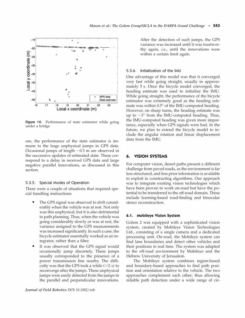
Figure 15. In �a� and �d�, blocks are classified by texture into path or nonpath. In �b� and �e�, sky blocks are removed andthree lines, arranged in a trapezoid, are fitted to the path blocks. The trapezoid is considered to represent the path. Finally,in �c� and �f�, the path boundaries are calculated at a given distance ahead of the vehicle �5 m, in this example� togetherwith the path center and heading angle.



system performance scored, on these sequences by ahuman observer. The path edge distance accuracywas computed by observing the position of the roadedge marks approximately 6 m in front of the ve-hicle. A frame was labeled incorrect if the path edgemarker at that location appeared to be more then30 cm ��18 pixels� away from the actual pathboundary. For straight paths, the perceived vanish-

ing point of the path was also marked, and our al-gorithm’s heading indicator was compared to thelateral position of this point.

On relatively straight segments with a comfort-ably wide path, our system reported availability�high system confidence� 100% of the time, whileproducing accurate path boundary locations 99.5%of the time. The mean angular deviation of the head-ing angle from the human marked vanishing pointwas 1.7°.

The second test clip is an example of more un-even terrains with elevation changes. Here, the ve-hicle passes through a dry river ditch �Figure 18�b��,where both the path texture and scene geometry aredifficult. When our vehicle is reaching the crest ofthe hill �Figure 18�h��, only a short segment of roadis visible. In this case, the system reported unavail-ability �low confidence� 8% of the time. When avail-able, however, the accuracy in boundary locationswas 98%.

The final clip contains a winding mountain pass�Figure 18�g��; difficult due to path curvature as wellas texture variation. Despite these, our system wasavailable throughout the clip, and achieved an accu-racy of 96% in detecting the path boundary.

6.1.4. Integration

The combination of the learning and geometric ap-proaches yields high-quality results with confidenceestimates suitable for integration into our controlsystems. Output from the Mobileye system—which

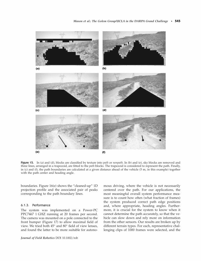
Figure 16. Projection-warp search: �a� Original imagewith the overlaid path boundary and focus of expansionresults, �b� the warped image, �c� texture gradients magni-tude, �d� projection: Vertical sum of gradients, and �e� pro-jection profile followed by convolution with a box filter.The two lines on top of the histogram mark the pathboundaries.

Figure 17. The camera is mounted inside a housing, atopa pole connected to the front bumper. This allows a betterfield of view than mounting the camera on the windshield.



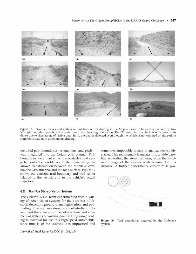
included path boundaries, orientations, and pitch—was integrated into the Golem path planner. Pathboundaries were marked as line obstacles, and pro-jected onto the world coordinate frame using theknown transformation between the Mobileye cam-era, the GPS antenna, and the road surface. Figure 19shows the detected trail boundary and trail centerrelative to the vehicle and to the vehicle’s actualtrajectory.

6.2. Toshiba Stereo Vision System

The Golem/UCLA Team experimented with a vari-ety of stereo vision systems for the purposes of ob-stacle detection, ground-plane registration, and pathfinding. Fixed-camera stereo is a well-studied prob-lem, and there are a number of academic and com-mercial systems of varying quality. Long-range sens-ing is essential for use in a high-speed automobile,since time is of the essence; it is impractical and

sometimes impossible to stop to analyze nearby ob-stacles. This requirement translates into a wide base-line separating the stereo cameras, since the maxi-mum range of the system is determined by thisdistance. A further performance constraint is pro-

Figure 18. Sample images and system output from 6 h of driving in the Mojave desert. The path is marked by twoleft-right boundary points and a center point with heading orientation. The “X” mark in �h� coincides with zero confi-dence due to short range of visible path. In �i�, the path is detected even though the vehicle is not centered on the path �acommon situation in autonomous driving�.

Figure 19. Trail boundaries detected by the Mobileyesystem.



cessing time, since latency can introduce dangerouserrors in path planning and control. Toshiba Re-search, in Kawasaki, Japan, developed a stereo sys-tem for on-road driving at high speeds, which weinstalled on Golem 2. Due to insufficient time, wedid not integrate the stereo system into the controlsystem of the vehicle before the GCE, but there is nodoubt that it has a high potential for successful au-tonomous driving. In this section, we describe thehardware configuration and implementation details.

6.2.1. Hardware Configuration

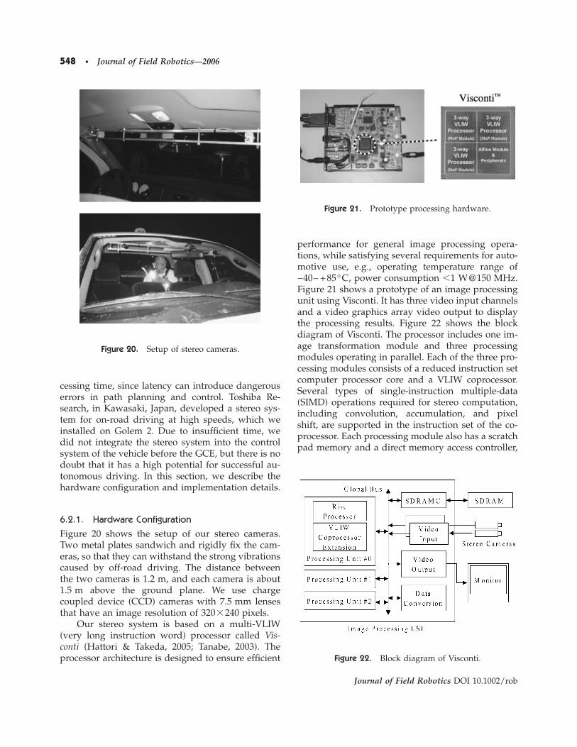
Figure 20 shows the setup of our stereo cameras.Two metal plates sandwich and rigidly fix the cam-eras, so that they can withstand the strong vibrationscaused by off-road driving. The distance betweenthe two cameras is 1.2 m, and each camera is about1.5 m above the ground plane. We use chargecoupled device �CCD� cameras with 7.5 mm lensesthat have an image resolution of 320�240 pixels.

Our stereo system is based on a multi-VLIW�very long instruction word� processor called Vis-conti �Hattori & Takeda, 2005; Tanabe, 2003�. Theprocessor architecture is designed to ensure efficient

performance for general image processing opera-tions, while satisfying several requirements for auto-motive use, e.g., operating temperature range of−40– +85°C, power consumption �1 W@150 MHz.Figure 21 shows a prototype of an image processingunit using Visconti. It has three video input channelsand a video graphics array video output to displaythe processing results. Figure 22 shows the blockdiagram of Visconti. The processor includes one im-age transformation module and three processingmodules operating in parallel. Each of the three pro-cessing modules consists of a reduced instruction setcomputer processor core and a VLIW coprocessor.Several types of single-instruction multiple-data�SIMD� operations required for stereo computation,including convolution, accumulation, and pixelshift, are supported in the instruction set of the co-processor. Each processing module also has a scratchpad memory and a direct memory access controller,

Figure 20. Setup of stereo cameras.

Figure 21. Prototype processing hardware.

Figure 22. Block diagram of Visconti.



so that memory access latency is hidden by double-buffering data translation.

6.3. Implementation Details

We adopt the sum of absolute differences �SAD� as amatching criterion within a 7�7 window, as SAD isless computationally expensive than other measuressuch as the sum of squared differences and normal-ized cross correlation. We also use a recursive tech-nique for the efficient estimation of SAD measures�Faugeras et al., 1993; Hattori & Takeda, 2005�. Inorder to compensate for possible gray-level varia-tions due to different settings of the stereo cameras,the input stereo images are normalized by subtrac-tion of the mean values of the intensities within amatching window at each pixel. Also, the variance ofintensities at each point is computed on the refer-ence image to identify those regions which have in-sufficient intensity variations for establishing reli-able correspondences.

As Visconti has one image transformation mod-ule and three processing modules operating in par-allel, task allocation for these modules is crucial toreal-time operation. For instance, the stereo rectifica-tion is a indispensable process that transforms inputstereo images so that the epipolar lines are alignedwith the image scan lines. The image transformationmodule carries out the stereo rectification, which isdifficult to accelerate by SIMD operations due to ir-regular memory access. Also, we divide a pair ofimages into three horizontal bands which are allo-cated to those three processing modules. Each ofthree areas has about the same number of pixels, sothat the computation cost is equally distributedacross the three modules.

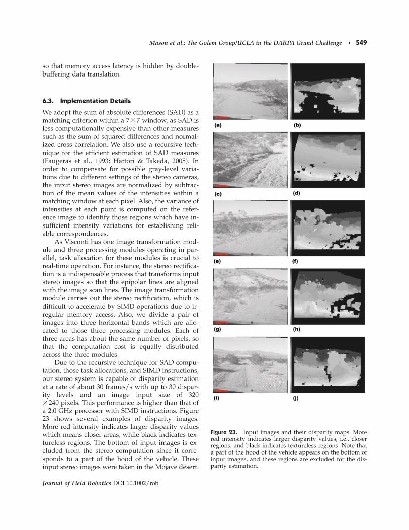
Due to the recursive technique for SAD compu-tation, those task allocations, and SIMD instructions,our stereo system is capable of disparity estimationat a rate of about 30 frames/s with up to 30 dispar-ity levels and an image input size of 320�240 pixels. This performance is higher than that ofa 2.0 GHz processor with SIMD instructions. Figure23 shows several examples of disparity images.More red intensity indicates larger disparity valueswhich means closer areas, while black indicates tex-tureless regions. The bottom of input images is ex-cluded from the stereo computation since it corre-sponds to a part of the hood of the vehicle. Theseinput stereo images were taken in the Mojave desert.

Figure 23. Input images and their disparity maps. Morered intensity indicates larger disparity values, i.e., closerregions, and black indicates textureless regions. Note thata part of the hood of the vehicle appears on the bottom ofinput images, and these regions are excluded for the dis-parity estimation.



7. RESULTS

Golem 2’s qualifying runs on the NQE obstaclecourse were among the best of the field, as shown inTable I, although we also failed on two runs for rea-sons discussed in Section 7.1.

Golem 2 raced out of the start chute at the 2005GCE in the seventh pole position. We knew that Go-lem 2 was capable of driving well at high speeds. Ourspeed strategy was that the vehicle would drive at themaximum allowed speed whenever this was below25 mph. If the recommended speed was greater than25 mph �implying that the maximum allowed speedwas 50 mph�, then Golem 2 would exceed the recom-mended speed, by small amounts at first, but moreand more aggressively as the race continued, until itwas always driving at the maximum legal speed, ex-cept, of course, when modulating its speed during aturn.

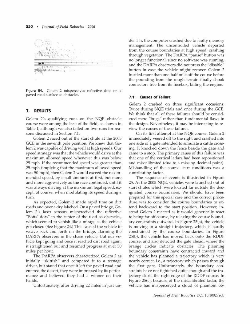
As expected, Golem 2 made rapid time on dirtroads and over a dry lakebed. On a paved bridge, Go-lem 2’s laser sensors misperceived the reflective“Botts’ dots” in the center of the road as obstacles,which seemed to vanish like a mirage as the vehiclegot closer. �See Figure 24.� This caused the vehicle toweave back and forth on the bridge, alarming theDARPA observers in the chase vehicle. But our ve-hicle kept going and once it reached dirt road again,it straightened out and resumed progress at over 30miles per hour.

The DARPA observers characterized Golem 2 asinitially “skittish” and compared it to a teenagedriver, but stated that once it left the paved road andentered the desert, they were impressed by its perfor-mance and believed they had a winner on theirhands.

Unfortunately, after driving 22 miles in just un-

der 1 h, the computer crashed due to faulty memorymanagement. The uncontrolled vehicle departedfrom the course boundaries at high speed, crashingthrough vegetation. The DARPA “pause” button wasno longer functional, since no software was running,and the DARPA observers did not press the “disable”button in case the vehicle might recover. Golem 2hurtled more than one-half mile off the course beforethe pounding from the rough terrain finally shookconnectors free from its fusebox, killing the engine.

7.1. Causes of Failure

Golem 2 crashed on three significant occasions:Twice during NQE trials and once during the GCE.We think that all of these failures should be consid-ered mere “bugs” rather than fundamental flaws inthe design. Nevertheless, it may be interesting to re-view the causes of these failures.

On its first attempt at the NQE course, Golem 2immediately veered off to the right and crashed intoone side of a gate intended to simulate a cattle cross-ing. It knocked down the fence beside the gate andcame to a stop. The primary cause of this failure wasthat one of the vertical ladars had been repositionedand miscalibrated �due to a missing decimal point�.Mishandling of the course start conditions was acontributing factor.

The sequence of events is illustrated in Figure25. At the 2005 NQE, vehicles were launched out ofstart chutes which were located far outside the des-ignated course boundaries. We should have beenprepared for this special case and the correct proce-dure was to consider the course boundaries to ex-tend backward to the start position. However, in-stead Golem 2 reacted as it would generically reactto being far off course, by relaxing the course bound-ary constraints outward. In Figure 25�a�, the vehicleis moving in a straight trajectory, which is hardlyconstrained by the course boundaries. In Figure25�b�, the vehicle has moved back onto the RDDFcourse, and also detected the gate ahead, where theorange circles indicate obstacles. The planningboundary constraints have contracted inward andthe vehicle has planned a trajectory which is verynearly correct, i.e., a trajectory which passes throughthe first gate. Unfortunately, the boundary con-straints have not tightened quite enough and the tra-jectory skirts the right edge of the RDDF course. InFigure 25�c�, because of the miscalibrated ladar, thevehicle has misperceived a cloud of phantom ob-

Figure 24. Golem 2 misperceives reflective dots on apaved road surface as obstacles.



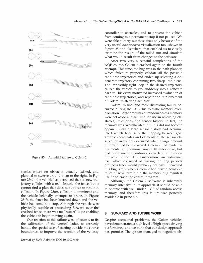
stacles where no obstacles actually existed, andplanned to swerve around them to the right. In Fig-ure 25�d�, the vehicle has perceived that its new tra-jectory collides with a real obstacle, the fence, but itcannot find a plan that does not appear to result incollision. In Figure 25�e�, collision is imminent andthe vehicle belatedly attempts to brake. In Figure25�f�, the fence has been knocked down and the ve-hicle has come to a stop. Although the vehicle wasphysically capable of proceeding forward over thecrushed fence, there was no “restart” logic enablingthe vehicle to begin moving again.

Our reaction to this failure was, of course, to fixthe calibration of the vertical ladar, to correctlyhandle the special case of starting outside the courseboundaries, to improve the reaction of the velocity

controller to obstacles, and to prevent the vehiclefrom coming to a permanent stop if not paused. Wewere able to carry out these fixes only because of thevery useful dashboard visualization tool, shown inFigure 25 and elsewhere, that enabled us to closelyexamine the results of the failed run and simulatewhat would result from changes to the software.

After two very successful completions of theNQE course, Golem 2 crashed again on the fourthattempt. This time, the bug was in the path planner,which failed to properly validate all the possiblecandidate trajectories and ended up selecting a de-generate trajectory containing two sharp 180° turns.The impossibly tight loop in the desired trajectorycaused the vehicle to jerk suddenly into a concretebarrier. This event motivated increased evaluation ofcandidate trajectories, and repair and reinforcementof Golem 2’s steering actuator.

Golem 2’s final and most distressing failure oc-curred during the GCE due to static memory over-allocation. Large amounts of random access memorywere set aside at start time for use in recording ob-stacles, trajectories, and sensor history. In fact, thememory was overallocated, but this did not becomeapparent until a large sensor history had accumu-lated, which, because of the mapping between geo-graphic coordinates and elements of the sensor ob-servation array, only occurred when a large amountof terrain had been covered. Golem 2 had made ex-perimental autonomous runs of 10 miles or so, buthad never made a continuous overland journey onthe scale of the GCE. Furthermore, an endurancetrial which consisted of driving for long periodsaround a track would probably not have uncoveredthis bug. Only when Golem 2 had driven across 22miles of new terrain did the memory bug manifestitself and crash the control program.

Although the Golem 2 software is inherentlymemory intensive in its approach, it should be ableto operate with well under 1 GB of random accessmemory, and therefore this failure was perfectlyavoidable in principle.

8. SUMMARY AND FUTURE WORK

Despite occasional problems, the Golem vehicleshave demonstrated a high level of high-speed drivingperformance, and we think that our design approachhas promise. The system managed to negotiate ob-

Figure 25. An initial failure of Golem 2.



stacles at speed using a relatively small amount ofcomputational power �a single 2.2 GHz laptop� andrelatively sparse laser range data.

The key drivers of this economically promisingperformance include a simplified computational ar-chitecture; using a combination of horizontally andvertically oriented ladars to reliably sense major ob-stacles while disregarding inessential details of theterrain; a fast heuristic planner which rapidly findssolutions in typical driving situations; and vehiclestate estimation using both an IMU and physical rea-soning about the constraints of the vehicle.

The “false” obstacles sometimes announced bythe ladar system were not entirely spurious, but gen-erally represented road markings or minor travers-able obstacles. Ideally, these would neither be ignorednor mistaken for nontraversable obstacles, but placedin a third category and treated appropriately by theplanning software. A future direction for the sensingsoftware is to improve the handling of these features,and also to improve the handling of moving ob-stacles.

ACKNOWLEDGMENTS

In addition to the authors of this paper, the GolemGroup included Jim Swenson, Jerry K. Fuller, JoshArensberg, Kerry Connor, Jeff Elings, Izaak Giber-son, Maribeth Mason, Brent Morgan, and Bill Cald-well, without whose invaluable technical assistancethe Golem vehicles would not have been possible.

The financial support of the Henry SamueliSchool of Engineering and Applied Sciences at theUniversity of California, Los Angeles, is gratefullyacknowledged. In addition, we received financialsupport and in-kind donations from a number ofother organizations, including BEI Technologies,Mobileye, NovAtel, Sick, and OmniStar.

REFERENCES

Alon, Y., Ferencz, A., & Shashua, A. �2006�. Off-road pathfollowing using region classification and geometricprojection constraints. Paper presented at the Interna-tional Conference on Computer Vision and PatternRecognition, New York.

Bornstein, J.A., & Shoemaker, C.M. �2003�. Army groundrobotics research program. In Unmanned ground ve-hicle technology V, Orlando, Florida. SPIE Proceed-ings Series, Volume 5083 �pp. 303–310�.

Coombs, D., Murphy, K., Lacaze, A., & Legowik, S. �2000�.Driving autonomously offroad up to 35 km/h. In Pro-ceedings of the IEEE Intelligent Vehicles Symposium,Dearborn, Michigan.

Dickmanns, E. �1997�. Vehicles capable of dynamic vision.Paper presented at the International Joint Conferenceon Artificial Intelligence, Nagoya, Japan �pp. 1577–1592�.

Dickmanns, E.D. �2004�. Dynamic vision-based intelli-gence. AI Magazine, 25�2�, 10–30.

Faugeras, O., Hots, B., Mathieu, H., Vieville, T., Zhang, Z.,Fua, P., Theron, E., Moll, L., Berry, G., Vuillemin, J.,Bertin, P., & Proy, C. �1993�. Real-time correlation-based stereo: Algorithm, implementations, and appli-cations �Technical Report No. 2013�. Sophia-Antipolis,France: INRIA.

Frazzoli, E., Dahleh, M.A., & Feron, E. �2002�. Real-timemotion planning for agile autonomous vehicles.AIAA Journal of Guidance, Control, and Dynamics,25�1�, 116–129.

Freund, Y., & Schapire, R.E. �1996�. Experiments with anew boosting algorithm. Paper presented at the Inter-national Conference on Machine Learning, Bari, Italy�pp. 148–156�.

Gelb, A. �1974�. Applied optimal estimation. Cambridge,MA: MIT Press.

Hattori, H., & Takeda, N. �2005�. Dense stereo matching inrestricted disparity space. In Proceedings of the IEEEIntelligent Vehicles Symposium, Las Vegas �pp. 118–123�.

Hong, T.H., Shneier, M.O., Rasmussen, C., & Chang, T.�2002�. Road detection and tracking for autonomousmobile robots. Paper presented at the SPIE 16th An-nual International Symposium on Aerospace/DefenseSensing, Simulation, and Controls, Orlando, Florida.

Kalman, R.E. �1960�. A new approach to linear filteringand prediction problems. Transactions of the ASME,82, 35–45.

Kalman, R.E. & Bucy, R.S. �1961�. New results in linearfiltering and prediction theory. Transactions of theASME, 83, 95–107.

Kavraki, L., Svestka, P., Latombe, J., & Overmars, M.�1996�. Probabilistic roadmaps for path planning inhigh-dimensional configuration spaces. IEEE Transac-tions on Robotics and Automation, 12, 566–580.

LaValle, S. �1998�. Rapidly-exploring random trees: A newtool for path planning �Technical Report No. TR 98-11�. Ames, IA: Iowa State University.

Rasmussen, C. �2002�. Combining laser range, color, andtexture cues for autonomous road following. Paperpresented at the IEEE International Conference on Ro-botics and Automation, Washington, DC.

Rogers, R.M. �2003�. Applied mathematics in integratednavigation systems. AIAA Education Series, 2nd ed.Reston, VA: AIAA.

Roundy, D. �2005�. David’s advanced revision control sys-tem �http: //darcs.net/ .

Tanabe, J. �2003�. Visconti: Multi-vliw image recognitionprocessor based on configurable processor. Paper pre-sented at the Custom Integrated Circuits Conference,San Jose, California �pp. 185–188�.



Urmson, C. �2005�. Navigation regimes for off-road driv-ing �Technical Report No. CMU-RI-TR-05-23�. Pitts-burgh, PA: Carnegie Mellon University, RoboticsInstitute.

Urmson, C., Anhalt, J., Clark, M., Galatali, T., Gonzalez, J.,Gowdy, J., Gutierrez, A., Harbaugh, S., Johnson-Roberson, M., Kato, H., Koon, P., Peterson, K., Peter-son, B., Smith, B., Spiker, S., Tryzelaar, E., & Whit-

taker, W. �2004�. High-speed navigation ofunrehearsed terrain: Red Team technology for GrandChallenge �Technical Report No. TR-04-37�. Pitts-burgh, PA: Carnegie Mellon University, RoboticsInstitute.

Welch, G., & Bishop, G. �1995�. An introduction to the Kal-man filter �Technical Report No. TR 95-041�. ChapelHill, NC: University of North Carolina at Chapel Hill.



Documents

The Golem Group/University of California at Los Angeles ... Golem Group/University of California at Los Angeles Autonomous Ground Vehicle in the DARPA Grand Challenge ... and allows