The Graph Crossing Number and its Variants: A Survey

The Graph Crossing Number and

its Variants: A Survey

Marcus Schaefer

School of Computing

DePaul University

Chicago, Illinois 60604, USA

[email protected]

Submitted: Dec 20, 2011; Accepted: Apr 4, 2013; Published: April 17, 2013

Third edition, Dec 22, 2017

Mathematics Subject Classifications: 05C62, 68R10

Abstract

The crossing number is a popular tool in graph drawing and visualization, but

there is not really just one crossing number; there is a large family of crossing number

notions of which the crossing number is the best known. We survey the rich variety

of crossing number variants that have been introduced in the literature for purposes

that range from studying the theoretical underpinnings of the crossing number to

crossing minimization for visualization problems.

1 So, Which Crossing Number is it?

The crossing number, cr(G), of a graph G is the smallest number of crossings requiredin any drawing of G. Or is it? According to a popular introductory textbook on combi-natorics [460, page 40] the crossing number of a graph is “the minimum number of pairsof crossing edges in a depiction of G”. So, which one is it? Is there even a difference?To start with the second question, the easy answer is: yes, obviously there is a differ-ence, the difference between counting all crossings and counting pairs of edges that cross.But maybe these different ways of counting don’t make a difference and always come outthe same? That is a harder question to answer. Pach and Tóth in their paper “WhichCrossing Number is it Anyway?” [369] coined the term pair crossing number, pcr, for thecrossing number in the second definition. One of the big open problems in the theory ofcrossing numbers is whether pcr(G) = cr(G) for all graphs G. If we don’t know whetherthey are the same, why do we see both notions called crossing number in the literature?

One potential source for the confusion between pcr and cr may be the famous crossingnumber inequality which states that for any graph G on n vertices and m edges we havecr(G) > c · m3/n2 for m > 4n and some constant c. The original proofs of this result

the electronic journal of combinatorics (2017), #DS21 1

are due independently to Ajtai, Chvátal, Newborn, Szemeredi [16] and Leighton [317].Leighton defines cr as pcr; since pcr(G) 6 cr(G), he is making a stronger claim; his proof isanalyzed in the section on crossing lemma variants below. The importance and influence ofLeighton’s paper may explain why some later papers using the crossing number inequalitywork with the pair crossing number [21, 451]. The danger, of course, is that the two notionsget confused; for example, Leighton [318, Theorem 1] proves that cr(G)+n > Ω(bw(G)2),where bw(G) is the bisection width of G (and G has bounded degree); his construction isfine for the standard crossing number, but does not work for pcr, the definition of crossingnumber he chose.1

Another influential crossing number result is Garey and Johnson’s proof that thecrossing number problem is NP-complete [203]; Garey and Johnson first mentioned theproblem as an open problem in their book on NP-completeness, where they write: “Openproblems for other generalizations of planarity include ‘Does G have crossing number Kor less, i.e. can G be embedded in the plane with K or fewer pairs of edges crossingone another?’ ” [202, OPEN3]. Clearly, they are defining what we now call the paircrossing number; in their later NP-completeness paper they write that K is the leastinteger so that “G can be embedded in the plane so that there are no more than K pair-wise intersections of curves representing edges (not counting the required intersectionsat common endpoints)” [203]. This is already somewhat ambiguous: does “pair-wise”mean that they only count the pairs, or that crossings count for each pair they belongto (which is relevant if more than two edges cross in a crossing). When they show thatthe crossing number problem lies in NP, it becomes clear that they mean the standardcrossing number and not the pair crossing number (for which membership in NP is nottrivial [410]).

This last example suggests another possible explanation for confusion among crossingnumbers: when trying to make precise what it means to count crossings, it is naturalto speak of pairwise crossings (to avoid problems with three edges crossing in the samepoint), and from there it is a short step to “pairs of edges crossing”.

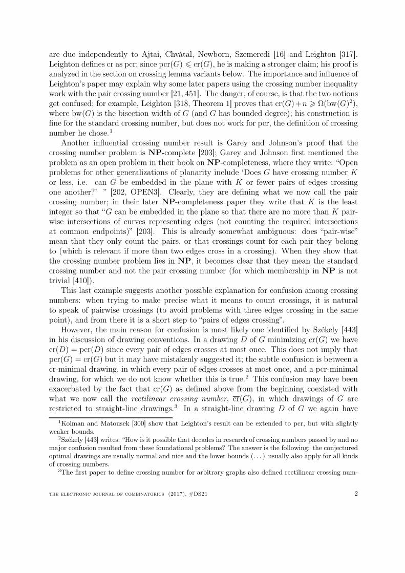
However, the main reason for confusion is most likely one identified by Székely [443]in his discussion of drawing conventions. In a drawing D of G minimizing cr(G) we havecr(D) = pcr(D) since every pair of edges crosses at most once. This does not imply thatpcr(G) = cr(G) but it may have mistakenly suggested it; the subtle confusion is between acr-minimal drawing, in which every pair of edges crosses at most once, and a pcr-minimaldrawing, for which we do not know whether this is true.2 This confusion may have beenexacerbated by the fact that cr(G) as defined above from the beginning coexisted withwhat we now call the rectilinear crossing number, cr(G), in which drawings of G arerestricted to straight-line drawings.3 In a straight-line drawing D of G we again have

1Kolman and Matousek [300] show that Leighton’s result can be extended to pcr, but with slightlyweaker bounds.

2Székely [443] writes: “How is it possible that decades in research of crossing numbers passed by and nomajor confusion resulted from these foundational problems? The answer is the following: the conjecturedoptimal drawings are usually normal and nice and the lower bounds (. . . ) usually also apply for all kindsof crossing numbers.

3The first paper to define crossing number for arbitrary graphs also defined rectilinear crossing num-


cr(D) = pcr(D) since every pair of edges can cross at most once, so it is natural to definethe crossing number for straight-line drawings as the number of pairs of edges that crossin a straight-line drawing (e.g. [475]); later authors may have dropped the straight-linerequirement without changing the way crossings are counted.4

Remark 1. As far as we know there are currently only three crossing number variants forwhich it is known that counting pairs of crossings as opposed to all crossings decreasesthe value of the crossing number: the constrained crossing number [353], the local cross-ing number (see that entry), and the geodesic crossing number (on a pseudosurface, seeFootnote 62).

Adjacent Crossings

There is some independent corroboration to Székely’s thesis that cr-minimal drawingsare at the root of the confusion between different crossing number notions; cr-minimaldrawings also have the property that adjacent edges do not cross, and sure enough thereare several instances in which researchers have ignored (sometimes at their peril) crossingsbetween adjacent edges. Tutte, in a slightly different context, famously remarked that“adjacent crossings are trivial and easily got rid of” [462].

To show that adjacent edges do not cross in a cr-minimal drawing, one typically refersto two pictures, like the left and middle pictures of Figure 1.

Figure 1: (left) adjacent crossing, (middle) removing adjacent crossing, (right) adjacentcrossing that’s hard to remove by local redrawing.

While this works fine for the standard crossing number (though even there one needsan additional argument that shows how to remove self-crossings that can be introducedwhen swapping arcs), this need not be the case for other crossing number notions. Forexample, consider the pair crossing number in the scenario depicted in the right picture ofFigure 1; swapping the arcs, or even just rerouting one of the arcs along the adjacent edgewill lead to an increase in the pair crossing number, so the simple local redrawing movescommon for cr do not seem to work. It is open whether a pcr-minimal drawing may have

ber [231].4Recent examples defining crossing number as pcr include textbooks in combinatorics [460, 451, 471],

and books in algorithms and complexity [41, 265, 36, 37].


crossings between adjacent edges (this question is equivalent to whether pcr < pcr+, seethe entry on pair crossing number in Section 3).

Even for the standard crossing number this is not the end of the story for adjacentcrossings. Here is a quote from a recent paper on Albertson’s conjecture: if G has chro-matic number at least r, then cr(G) > cr(Kr).

“A crossing of two edges e and f is trivial if e and f are adjacent or equal,and it is non-trivial otherwise. A drawing is good if it has no trivial crossings.The following is a well-known easy lemma.

Lemma 1.1. A drawing of a graph can be modified to eliminate all ofits trivial crossings, with the number of non-trivial crossings remaining thesame.” [362]

The independent crossing number, cr−(G), only counts crossings occurring betweenindependent edges. If Lemma 1.1 were true, it would imply that cr− = cr, a questionthat’s open to the best of our knowledge.5 Fortunately, the use of Lemma 1.1 could beeliminated in this case [361], but wouldn’t it be nice if we could establish cr− = cr and nothave to worry about adjacent crossings anymore? The left and middle picture of Figure 1explain why Lemma 1.1 looks so convincing: crossings between adjacent edges can easilybe removed by local redrawing, but the right picture shows that this can create crossingsbetween non-adjacent pairs of edges. A proof of a result like Lemma 1.1 will require amore global approach.

Question 2. Here are two simple-looking problems that illustrate our lack of understand-ing of adjacent crossings. (i) Can subdividing an edge change cr− of a graph? (ii) Supposea graph can be drawn on a surface so that all crossings in the drawing are between ad-jacent edges. Can the graph be embedded in that surface? An answer to the secondquestion is known for the plane and the projective plane by virtue of the Hanani-Tuttetheorems for those surfaces [376], but not for any other surface.6 The first question isopen.

While not nearly as common as the pcr versus cr problem, cr is occasionally defined asthe smallest number of independent crossings; this may again be due to the fact that forstraight-line drawings, adjacent edges do not cross. For example, Moon [346] in one of theearliest papers on crossing numbers defines what amounts to the independent (geodesic)spherical crossing number which equals the geodesic spherical crossing number, since

5Start with a cr−-minimal drawing. By the lemma, all trivial crossings can be eliminated, only leaving“non-trivial” crossings, that is, crossings that count towards cr, so cr of the resulting drawing is at mostcr−. In the other direction, cr− 6 cr follows from the definition.

6The Hanani-Tutte theorem for a surface Σ is true if every graph which can be drawn on Σ so that notwo independent edges cross an odd number of times is embeddable in Σ. The Hanani-Tutte theorem isknown to be true for the plane (sphere) [120, 462] and the projective plane [376]. It is not known to betrue for any other surface, and it has been announced that it fails for surfaces of genus 4 and higher [196].In terms of crossing numbers, the Hanani-Tutte condition can be expressed as saying that iocrΣ(G) = 0implies that crΣ(G) = 0 for all graphs G.


geodesics representing adjacent edges do not cross on the sphere. Nahas [354] definesthe crossing number of Km,n as cr−(Km,n). Papers on crossing minimization via linearprogramming also often ignore variables that encode crossings between adjacent edges.This is fine, of course, as the resulting program enforce that adjacent edges do not cross;otherwise, they would compute cr−.

Remark 3. As far as we know there are only two crossing number notions for whichthe independent variant is known to differ from the regular variant, namely the oddand the algebraic crossing number: there are graphs G for which iocr(G) < ocr(G) andiacr(G) < acr(G) [197]. The same paper also shows that prohibiting crossings betweenadjacent edges in monotone drawings can lead to an increase in the monotone odd crossingnumber. The same is true for the local crossing number, see Footnotes 72 and 74, andthe simultaneous crossing number, see Footnote 100. For directed graphs, the bimodalcrossing number may require crossings between adjacent edges in an optimal drawing.

Crossing Lemma Variants

The crossing lemma, or crossing number inequality, established independently by Ajtai,Chvátal, Newborn, Szemeredi [16] and Leighton [317], is one of the most celebrated (andfamous) results on crossing numbers.7 In its original form, it shows that cr(G) > c·m3/n2,where n = |V |, and m = |E|. How does it fare for other crossing number variants, andpair and odd crossing number in particular? Crossing lemmas for other variants are listedin the compendium below.

The usual probabilistic proof of the crossing lemma for a crossing number γ proceedsin three steps: first, we observe that if γ(G) = 0, then G is planar, so Euler’s formulaapplies, and m 6 3n − 6, where n = |V (G)|, m = |E(G)|. In a second step, we arguethat we can remove at most γ(G) edges from G to reduce γ to 0, so m− γ(G) 6 3n− 6,and, hence, γ(G) > m − 3n. In a third step, we consider a random subgraph G′ ofG, keeping each vertex with probability p. The expected number of vertices and edgesin G′ = (V ′, E ′) are E(|V ′|) = pn and E(|E ′|) = p2m. Fix a γ-minimal drawing D ofG. Assuming each crossing in D which contributes to γ is caused by two independentedges, a crossing is associated with four endpoints. For the crossing to survive in D′, theinduced drawing of G′, all four endpoints have to be kept, so E(γ(G′)) 6 p4γ(G). NowG′ fulfills γ(G′) > |E ′| − 3|V ′| (by the second step), so, taking expected values, we getp4γ(G) > p2m − pn, or γ(G) > mp−2 − np−3 (assuming p > 0). Choosing p = 4n/mimplies that γ(G) > 1/64m3/n2, as long as m > 4n (which we need so p 6 1).

For γ = cr, this proof works just fine, and it’s been claimed in the literature (e.g.[365]) that this proof also works for pair and odd crossing numbers. But there are twosubtle problems. Consider the case γ = pcr, the case claimed by Leighton [317]: in thesecond step, the pcr-minimal drawing D may contain crossings between dependent edges,and those contribute to pcr. Since we do not know how to remove dependent crossingsin general without increasing pcr(D), we have to take dependent crossings into account;

7For a very readable introduction, see Terence Tao’s blog enty [450], which also discusses applicationsto incidence geometry and sum-product estimates.


since those survive with probability p3, we would get a substantially worse bound thanΩ(m3/n2) on pcr(G). Alon [21], and Tao and Vu in their book on additive combina-torics [451] circumvent this problem by working with pcr−, the independent pair crossingnumber, in which only the number of crossings of independent pairs of edges are counted.However, for that crossing number the second step is no longer obvious: if we have adrawing D with k independent pairs of edges crossing, then removing k edges yields adrawing in which all remaining crossings are dependent. Is that graph planar? The an-swer is yes, but it requires the Hanani-Tutte theorem (see Footnote 6) to prove so (atleast we are not aware of a direct proof).

Remark 4. Since the Hanani-Tutte theorem is not known to be true for the torus, thismeans that we do not currently have a proof of the crossing lemma for pcr or pcr− on thetorus. A positive answer to Question 2 (ii) would be sufficient to settle the problem. Forthe standard crossing number, extensions of the crossing lemma to arbitrary surfaces areknown [429].

Pach and Tóth [369] work with γ = ocr, the odd crossing number, which only countspairs of edges crossing an odd number of times. They use Hanani-Tutte in the first andsecond steps, but in the third step again assume that a crossing is associated with fourendpoints, which may not be the case for ocr. However, their proof is essentially correctif read for γ = iocr, the independent odd crossing number, which counts the numberof independent pairs of edges crossing an odd number of times. For iocr, the Hanani-Tutte theorem guarantees that we can remove iocr(G) edges from G to make G planar,ensuring the correctness of the first and second steps. And since iocr by definition onlycounts independent pairs, the argument in the third step also works. We conclude thatiocr(G) > 1/64m3/n2, as long as m > 4n. Since ocr, pcr, and pcr− (as well as acr andiacr) are all bounded below by iocr, this immediately proves the crossing lemma for allthese variants. The constant c = 1/64 in these cases is weaker than what is currentlyknown for cr, but seems hard to improve [365, Remark 4.2], though it was recently shownc = 1/34.2 will work for pcr+ [11].

Conclusion

We are forewarned that there is some subtlety to defining the crossing number, but ratherthan seeing this as an issue, this gives us an opportunity. János Pach once said, ineffect, “we don’t need more crossing numbers, we need fewer crossing numbers”. As alook at the compendium will show it may be too late for that. Some crossing numbervariants may have arisen by mistake, but most were defined with a specific purpose inmind. This purpose may be theoretical, aimed at developing a theory of crossing number(as Tutte [462] did with his crossing chains and iacr) or it may be practical, aimed atimproving the layout of graphs (as in the Metro-line crossing minimization problem).The recent growth of graph drawing research and crossing minimization problems forvery specific visualization tasks is important evidence for that. Some variants, such asthe local crossing number or the maximum rectilinear crossing number, are so fundamentalthat they have been rediscovered over and over again under various names.


This survey of crossing number variants follows two main goals: to collect as manydifferent types of crossing number variants from the literature as possible (unifying pre-sentations and names), and to attempt a systematic description of what makes a crossingnumber. The results of this second step are presented first, in Section 2. The results ofthe first step are collected in the Compendium in Section 3. Originally, the paper was tocontain a section on the history of the crossing number, however, Beineke and Wilson’s“Early History of the Brick Factory problem” [60] and Székely’s “Turán’s brick factoryproblem: the status of the conjectures of Zarankiewicz and Hill” make this part mostlysuperfluous.

Remark 5 (Forerunners of Crossing Minimization in Sociology). David Eppstein [170]discovered the earliest known references to (general) crossing minimization.8 They comefrom sociology, more specifically the area of sociometry which is concerned with measuring(and depicting) social relationships: in discussing sociograms (essentially graphs), Bron-fenbrenner [87] in 1945 writes that “The arrangement of subjects on the diagram, whilehaphazard in part, is determined largely by trial and error with the aim of minimizingthe number of intersecting lines”. Sociograms were introduced in J.L. Moreno’s “WhoShall Survive” [347] in 1934, however, the first edition of that book, while containingmany interesting graph visualizations, does not seem to discuss crossing minimization. Inthe later, 1953, edition [348],9 there is an interesting paragraph which reads: “A readablesociogram is a good sociogram. To be readable, the number of lines crossing must be min-imized.” This mantra occurs repeatedly in the literature on sociograms, and at least oncein an earlier paper by Borgatta [82] who writes: “A readable diagram is a good diagram.To be readable, the number of lines crossing must be minimized. This may be taken asa primary principle in the construction of inter-action diagrams; the fewer the number oflines crossing, the better the diagram. The problem, then, is to find the procedure whichbest minimizes the number of lines that cross in a diagram.” Borgatta then outlines amulti-stage heuristic for crossing minimization (start with a small number of high-degreevertices, drawn far apart, add vertices by decreasing degree, redraw diagram to improvedrawings of subgroups), and illustrates his method by working out an example on 26vertices and 43 edges, shown in Figure 2; his final drawing uses two crossings (which isoptimal, since his graph contains two disjoint copies of K5).

The earliest reference (found so far) on crossing minimization seems to be a 1940paper by Northway [359] in which she suggests the use of radial layouts; vertices (schoolchildren) are placed at various distances from a center based on some quantity (theirscores); directed edges between them are drawn as straight-line arrows. She writes that“it has been convenient to use counters [. . . ]. These are moved in the circles to whichtheir score belongs and arranged to get the best “fit” among the individuals, i.e., tohave as few long lines and crossing lines as possible.” She also suggests that groupingvertices by some characteristic (in her example, sex), simplifies this task. These quotes

8There are earlier references to crossing minimization when it comes to specific families of graphs [123,297, 439], but none that are as general as these.

9This edition is available online at http://www.asgpp.org/docs/WSS/wss%20index/wss%20index.

html


http://www.asgpp.org/docs/WSS/wss%20index/wss%20index.html

http://www.asgpp.org/docs/WSS/wss%20index/wss%20index.html

(a) (b)

Figure 2: Maybe the first published instance of a crossing minimization, reducing 16crossings in (a) to the optimal 2 crossings in (b). Taken (with permission) from a 1951article in the journal “Group Psychotherapy” by Edgar F. Borgatta [82].

are quite remarkable, and one wonders whether there is more early material on crossingminimization that is unknown in the mathematical literature.

One aspect that remains to be studied, is the history of knot crossing numbers andtheir influence (or not) on graph crossing numbers. When it comes to methods of countingcrossings, it seems that knot crossing numbers led the way; e.g. Tutte’s theory of cross-ing numbers is based on counting crossings algebraically, as one would for the algebraiccrossing number in knot theory, and as Gauß would have done hundreds of years ago [206,page 271–279].

Remark 6 (Axioms). What makes a crossing number a crossing number? We have chosena descriptive/extensional approach for this survey, however, the material collected heremay at some point make a basis for a prescriptive/intensional approach. As far as we knowthere has never been an attempt to axiomatize the notion of crossing number, either asthe standard crossing number or as the family of crossing number variants. Although notplentiful, there are some candidate axioms based on common crossing number properties.

Embeddability Crossing numbers are generally considered to be “measures of non-


planarity” or non-embeddability. It seems natural then to require that if γΣ(G) = 0for some crossing number γ in surface Σ, then G is embeddable in Σ. Let us callthis the embeddability axiom. For the standard crossing number this is true by defi-nition (on any surface). For the independent odd crossing number it amounts to theHanani-Tutte theorem (which is only known for the plane and the projective plane,see Footnote 6). For the confluent crossing number and the string crossing num-ber, the embeddability axiom fails (complete graphs have confluent embeddings andthere are non-planar string graphs). A stronger, quantitative version of this axiomwould require that the removal of at most γ(G) edges from G makes G planar. Theintuition behind this strengthened version is that each crossing is caused by twoedges, so a crossing can be eliminated by removing one of the participating edges.This axiom holds for the standard crossing number by definition (on any surface),and for the pair crossing number. It also holds for the independent odd crossingnumber in the plane and the projective plane, by the Hanani-Tutte theorem (Foot-note 6), but, by [196] it fails on surfaces of genus 4 and higher. It also fails for thedegenerate crossing number, in which more than two edges can cross in a crossing,and for any of the crossing numbers based on maximization.

Embedding By the same “measure of non-planarity” argument, a graph G that can beembedded in a surface Σ should have crossing number γΣ(G) = 0. Let us call thisthe embedding axiom. This axiom is trivially true for most crossing number variants,although there are some notable exceptions including crossing numbers defined viamaximization (maximum crossing number, maximum rectilinear crossing number)and crossing numbers that require certain drawing conventions (e.g. bimodal, bipar-tite, convex, and orchard crossing numbers). For the rectilinear crossing number,the axiom amounts to Fary’s (or Wagner’s or Steinitz’s) theorem. It appears to bean open problem whether the axiom holds for the geodesic crossing number on othersurfaces.10

Subgraph Monotonicity The subgraph monotonicity axiom requires that if G is a sub-graph of H , then γ(G) 6 γ(H). This is true (and trivial) for nearly all crossingnumber variants. We are aware of only two provable exceptions, the triple crossingnumber, for which triple-cr(K5,3) = ∞ while triple-cr(K6,3) = 2 [449], and the con-fluent crossing number (all complete graphs have confluent crossing number 0). Forthe maximum crossing number, monotonicity is a well-known open problem evenif G is required to be an induced subgraph of H [395]. A stronger requirementis topological minor monotonicity: if G is a subdivision of a subgraph of H , thenγ(G) 6 γ(H). This is still true for a large number of crossing numbers, but is notknown to hold for any of the independent crossing number variants, like cr−, andtypically fails for alternative representations (like the confluent crossing number).In contrast, most crossing numbers do not satisfy minor-monotonicity which has ledto the definition of the minor (or minor-monotone) and the genus crossing numbers.

10An announcement of a solution in [454, page 312] may have been in error [455].


Surface Monotonicity The surface monotonicity axiom requires that if surface Σ hassmaller genus than surface Γ, then γΣ > γΓ. We are not aware of any crossingnumber that does not fulfill this axiom. One could imagine sharper quantitativeversions of this axiom, for example if Σ has smaller genus than Γ, then γΣ(G) >γΓ(G) unless γΣ(G) = 0.

One can imagine further axioms, for example based on what may be called the spectrumof the crossing number of a graph G: γ(D) : D is a drawing of G. This notion hasoccasionally been studied, e.g. [198, 384] for the maximum crossing number, or [247] forthe edge crossing number. Harborth [244] showed that the spectrum of K14 under cr is nota subset of the spectrum of K14 under the 2-page crossing number bkcr2, and conjecturedthat K14 is the smallest complete graph for which the spectra of cr and bkcr2 differ.11

It is probably unreasonable to expect an axiomatization of the (standard) crossingnumber; however, it may be reasonable to attempt to axiomatize sufficiently many stan-dard properties of the crossing number that would show why many of them allow a crossinglemma. Or why many of them can be bounded within each other.

2 A Systematic Approach

In this section we want to take a systematic approach to crossing number variants. Thediscussion is based on the crossing number notions collected from the literature and pre-sented in Section 3, and the reader is asked to look for definitions there if they are notgiven in this section. Before reviewing crossing numbers, we begin with a discussion ofcrossings themselves.

What is a crossing? Typically, a crossing is defined to be a common interior point oftwo edges; hence, a shared endpoint (of two adjacent edges) is not considered a crossing.This distinguishes a crossing from an intersection of two edges.12

The definition as given also distinguishes a crossing from the point in the plane atwhich the crossing occurs (and this is good). The definition does, however, include pointsin which two curves touch; this is of no consequence for the standard crossing number sincein crossing-minimal drawings no touching points occur, but for other variants, e.g. theodd crossing number, counting touching points as crossings would trivialize the notion.For Kleitman [294] a crossing requires that the two edges involve actually cross. Thisrequirement leads to other issues if not handled carefully: take a drawing of K5 with asingle crossing and replace the crossing with a short line segment (so the two edges involvedin the crossing run parallel for a short stretch). According to Kleitman’s definition thisdrawing is free of crossings (even though it has an infinite number of intersection points).This suggests the importance of restricting drawings to drawings with a finite number ofintersection points (which is what we will do) which causes a slight inconvenience when

11Harborth mentions an unpublished paper that seems to establish significant parts of this conjecture.12One subtlety already: it excludes from the notion of crossing any intersection occurring when an

edge passes through a vertex, as opposed to ending there. Such intersections are typically prohibited, butwhat happens if we allow them?


dealing with confluent drawings: in confluent drawings of graphs edges seem to overlapheavily. We resolve this by looking at confluent drawings not as drawings of the edgesand vertices of the graph, but as a drawing of branches and switches that represent theunderlying graph.

We return to a more formal definition of crossing in Section 2.2.1 after discussing basicdrawing conventions.

Figure 3: Drawing of K8 from de la Vera Cruz’ Recognitio Summularum with ribbonscrossing through each other. The image is taken from the online (public domain) versionof the book available through Primeros Libros at http://www.primeroslibros.org/

browse.html. Page 36 contains the drawing of K8, page 57 contains a drawing of K4,4−e.

Remark 7 (Drawing Crossings). How do we draw a crossing? The most common way isto simply let the curves representing the edges cross, preferably at a large angle (RACdrawings require right angles); alternatively one can draw crossings as bridges or by usingedge casing; see “Edges and switches, tunnels and bridges” by Eppstein, van Kreveld,Mumford and Speckmann [173]. There may be more options in alternative styles; forexample, if vertices are represented by disks and edges as ribbons with boundary, thencrossings can be visualized by ribbons passing above or below each other, see for examplethe 16th century drawing of K12 in [310, Figure 6] which has both vertex and edge labels(illustrating a modal square of opposition). Alonso de la Vera Cruz uses an interestingtwist to visualize K8 (in his 1554 Recognitio Summularum, again for a square of oppo-sition). He not only has ribbons passing above and below each other, but also througheach other, see Figure 3; for background on the book, see [95].

Most of the research on crossing numbers seems to have been done in English, butthere are terms for crossings and crossing numbers in other languages. In German there is


http://www.primeroslibros.org/browse.html

http://www.primeroslibros.org/browse.html

Kreuzung, Schnitt and Doppelpunkt for crossing and Kreuzungszahl for crossing number.13

In French, we have points d’intersection [465] and croisement for crossings14 and nombresde croisement for crossing number. In Italian there is incrocio for crossing and numerod’incrocio for crossing number.

2.1 A General Notion of Crossing Number

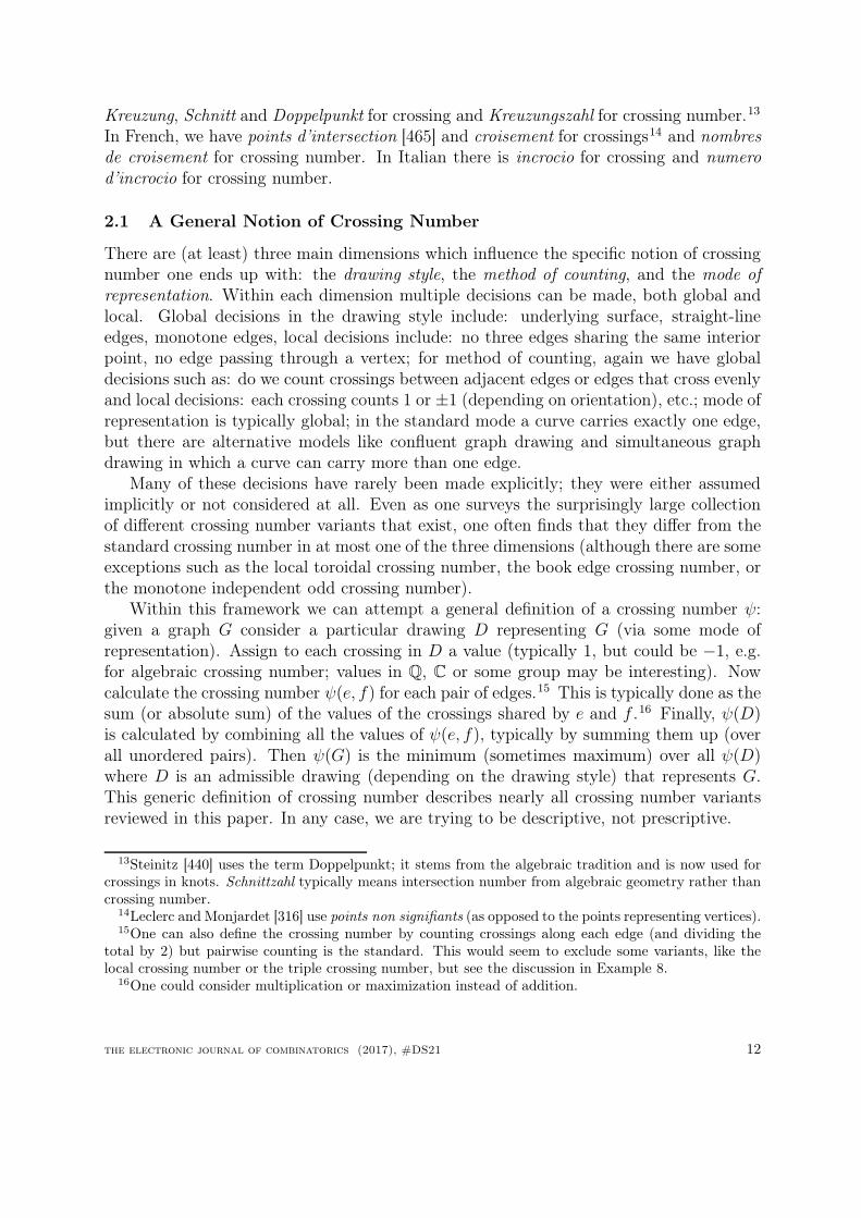
There are (at least) three main dimensions which influence the specific notion of crossingnumber one ends up with: the drawing style, the method of counting, and the mode ofrepresentation. Within each dimension multiple decisions can be made, both global andlocal. Global decisions in the drawing style include: underlying surface, straight-lineedges, monotone edges, local decisions include: no three edges sharing the same interiorpoint, no edge passing through a vertex; for method of counting, again we have globaldecisions such as: do we count crossings between adjacent edges or edges that cross evenlyand local decisions: each crossing counts 1 or ±1 (depending on orientation), etc.; mode ofrepresentation is typically global; in the standard mode a curve carries exactly one edge,but there are alternative models like confluent graph drawing and simultaneous graphdrawing in which a curve can carry more than one edge.

Many of these decisions have rarely been made explicitly; they were either assumedimplicitly or not considered at all. Even as one surveys the surprisingly large collectionof different crossing number variants that exist, one often finds that they differ from thestandard crossing number in at most one of the three dimensions (although there are someexceptions such as the local toroidal crossing number, the book edge crossing number, orthe monotone independent odd crossing number).

Within this framework we can attempt a general definition of a crossing number ψ:given a graph G consider a particular drawing D representing G (via some mode ofrepresentation). Assign to each crossing in D a value (typically 1, but could be −1, e.g.for algebraic crossing number; values in Q, C or some group may be interesting). Nowcalculate the crossing number ψ(e, f) for each pair of edges.15 This is typically done as thesum (or absolute sum) of the values of the crossings shared by e and f .16 Finally, ψ(D)is calculated by combining all the values of ψ(e, f), typically by summing them up (overall unordered pairs). Then ψ(G) is the minimum (sometimes maximum) over all ψ(D)where D is an admissible drawing (depending on the drawing style) that represents G.This generic definition of crossing number describes nearly all crossing number variantsreviewed in this paper. In any case, we are trying to be descriptive, not prescriptive.

13Steinitz [440] uses the term Doppelpunkt; it stems from the algebraic tradition and is now used forcrossings in knots. Schnittzahl typically means intersection number from algebraic geometry rather thancrossing number.

14Leclerc and Monjardet [316] use points non signifiants (as opposed to the points representing vertices).15One can also define the crossing number by counting crossings along each edge (and dividing the

total by 2) but pairwise counting is the standard. This would seem to exclude some variants, like thelocal crossing number or the triple crossing number, but see the discussion in Example 8.

16One could consider multiplication or maximization instead of addition.


Example 8. Let us check some of the crossing number variants to test the bounds of ourgeneral crossing number notion. For definitions, see the compendium.

Natural fits. The degenerate crossing number fits the general definition above: a cross-ing shared by k edges is weighted as 1/

(k2

). Independent crossing numbers can be

captured by assigning values of 0 to crossings between adjacent edges. The Rule+ variants introduced by Pach and Tóth [368] are captured in the drawing style:adjacent edges are not allowed to cross (alternatively, we could assign a value of ∞to each adjacent crossing). The triple crossing number (in which all crossings haveto be triple crossings) can be captured by pairwise counts (each triple crossings givesthree double crossings; since only triple crossings are allowed we can divide by 3 toget the triple crossing number). The pair crossing number maximizes (rather thanadds) the number of crossings along each pair of edges.

Acceptable fits. The local crossing number would be a more natural fit for countingcrossings edge-wise (as opposed to pairwise), but it can be made to fit the generaldefinition. It is expressible as maxe∈E

∑f∈E cr(e, f).

Forced fits. The minor crossing number can be made to fit the general description ofcrossing number above, albeit with some force: say a drawing D represents G if Dis a drawing of a graph containing G as a minor. One could question whether thisis a natural interpretation, but we decided to include this notion. The degenerateand bundled crossing numbers can also be made to fit the definition by defining anintermediate notion of drawing.

Not a fit. The skewness of a graph, the smallest number of edges that need to be removedfrom a graph to make it planar, does not fit the general definition of crossing numbergiven above. One can debate whether skewness is a crossing number variant, butwe decided to exclude it. It is easy to abbreviate the standard definition of crossingnumber to the point where it incorrectly defines a notion similar to skewness, e.g. “Isthe crossing number of G 6 K? i.e. can G be embedded in the plane in such a waythat no more than K edges cross?” [253], see the edge crossing number. Anothernotion that is not covered by the general description is the nodal crossing numberwhich is similar to the local crossing number, but looks at the total number ofcrossings with any edge incident to a vertex, and then maximizes over all vertices.One could think of it as a local crossing number for hypergraphs. Even though itdoes not fit our general model, we decided to include it because of its ties to thelocal crossing number.

Let us next review some of the options available for creating a crossing number withinthe three dimensions we identified; we start with a discussion of drawing styles, followedby methods of counting, and modes of representation.


2.2 Drawing Styles

In this section we discuss different drawing styles; we make a rather rough distinctionbetween basic drawing properties that are often taken to be part of the very definitionof a drawing, sometimes called a good drawing and what may more properly be called astyle of drawing (Section 2.2.2). We treat drawing surfaces separately in Section 2.2.3.

2.2.1 The Basics

A drawing stripped of any mystic ballast is just a mapping of a graph (vertices and edges)to a surface. With this generous definition of drawing, the whole graph could map to asingle point, losing all structure. There has not been much discussion of what assumptionsto make on a drawing, Eggleton’s thesis [163] is one of the rare places in which some ofthese issues are brought up. We first discuss issues related to drawing vertices and

edges.

An edge is represented by a curve. But what type of curves do we allow? Do wewant a curve to be connected? In the work on odd and algebraic crossing num-bers edges are often split into multiple components temporarily. Becker, Eick andWilks [59] suggested “line shortening” for geometric drawings: only the ends of edgesare drawn (without further restrictions this removes all crossings, see [88] for a re-cent paper). If we require the curve to be connected (but not path-connected), wecan get some anomalies, for example Kratochvíl [306] notes that every graph is astring graph if strings are allowed to be arbitrary connected curves (string graphsare intersection graphs of simple curves in the plane). So we should require edges tobe simple plane curves, which are homeomorphic images of the unit interval. Thisis the typical choice when defining a drawing. However, it does preclude edges fromcrossing themselves which may be desirable in some contexts. We discuss the issueof self-intersections below. For practical reasons, it may make sense to “fatten up”edges, we discuss this possibility below together with vertex representations.

Vertices are endpoints of the edge. Often edges are defined as open arcs at whichpoint one has to specify that the points representing the vertices of the edge occurat (opposite) ends of the arc. One could easily imagine a drawing of K5 with the 5endpoints as isolated points and 10 parallel arcs representing the edges (maybe withthe ends of the arcs labeled by the names of the vertices). One could also considerthis a special case of allowing a vertex to be represented by multiple points (seebelow).

Vertices are represented by points. Suppose we represent vertices by disks and onlyrequire edges to attach at the boundary of the disk. This idea was (ab)used byDudeney in his original solution to the Gas, Water, Electricity problem [148, Prob-lem 251] which essentially asks for a crossing-free drawing of K3,3: Dudeney has thefinal path—which would cause a crossing—pass through one of the houses (vertices)which he drew as rectangles. Suppose we do allow edges to pass through vertices.


If we allow such crossings for free (as Dudeney suggests) we trivialize the notion ofcrossing number: every graph can be represented so that a vertex is a disk, edgesend on the boundary of the disk representing their endpoint, edges are allowed topass through the disk, and no two edges cross. However, we could consider allowingedges to pass through vertices for a cost. As far as we know no such notion hasbeen investigated, although there are crossing numbers which count crossings otherthan edge crossings (e.g. the spine crossing number).

One reason to relax the requirement that vertices be points may be that the ver-tices represent objects with internal structure that has to be captured. Eades andLai [159, 311] called these practical graphs, and suggested a two-step approach: firstuse a general layout algorithm for the abstract graph, and then, in a second step,lay out the graph with vertices having various shapes; the goal of the second step isto avoid or remove overlap between vertices and vertices with edges. Waddle [469]discusses port diagrams (in which vertices are rectangles, and edges attach at a port)to visualize data structures; his goal is to find drawings that avoid crossings withinvertices, also see [293, 417]. Duncan, Efrat, Kobourov and Wenk [154] investigatedplanar drawings with “fat edges”, where vertices are disks and edges have thick-ness.17 Van Kreveld [309] suggested the notion of bold drawings in which verticesare disks and edges are rectangles. In computational biology, such drawings havebeen suggested for visualizing chromosomes [188]. Medieval scholars used a similarstyle (vertices as disks, edges as ribbons) to visualize squares of opposition (in logic)as we saw in Figure 3. Other choices for representing vertices include curves—thestring crossing number is based on that idea—and graphs: If we minimize the cross-ing number by allowing vertices to be replaced by arbitrary connected graphs, weobtain the minor crossing number.

Each vertex is represented by a single point. One can easily imagine a vertex be-ing represented by multiple points. For example, how would the standard crossingnumber be affected if every vertex could be represented by two points (which to-gether are incident to all the edges incident to the original vertex), we could callthis the duplicate crossing number.18 This seems nearly the same (is it?) as askingfor the crossing number of the graph on an n-spindle, the pseudosurface resultingfrom a sphere by pinching (identifying) n pairs of distinct points. If n = |V (G)|,then the duplicate crossing number of G is at most the crossing number of G on then-spindle, since we can simply pinch every vertex with its duplicate. The duplicatecrossing number also resembles the biplanar crossing number: here too every vertexis represented by two points, but the duplicate points live on a different sphere, sothere cannot be an edge between the original and the duplicate vertices. There is re-search on whether graphs can be planarized by multiplying vertices, following ideas

17The discussion of edges with width and points with extension is much older in “practical geometry”;Hjlemslev [255, 256] attempted an axiomatization, which earned him the scorn of Wittgenstein [480,Gesichtsraum, p.59].

18Bertin [68, Figure 19, p.270] suggests using diagrams in which every vertex is duplicated.


of Fellows and Negami from the 1980s on planar emulators and covers, see [112]for a recent overview. Finally, one can turn a cyclic layout into a linear layoutby repeating one of the layers (for example, turning a cyclic level crossing numberproblem into a k-layer crossing number problem).19

Different vertices are mapped to different locations. This is generally assumed forgraph drawings though there are some exceptions. For example, when speaking ofrealizing a linkage one does not care about vertex overlap, and the definition of aEuclidean graph similarly allows multiple vertices at the same location. For cross-ing numbers, this has not been a major issue; the only crossing number that allowsvertex overlap is the diagonal crossing number introduced by Negami (though onecould argue that the simultaneous crossing number also is an instance). For visual-ization purposes one could imagine a model in which different vertices are allowed atthe same location as long as edges adjacent to a particular vertex are consecutive inthe rotation. Buchheim, Jünger, Menze, Percan [92] suggest the notion of bimodalcrossing number which has some similarity.

Edges are not allowed to pass through vertices. Again this restriction is naturallyviolated by linkages and Euclidean graphs. For example, a triangle with side-lengths1, 1 and 2 can only be realized if we allow the edge of length 2 to pass through thevertex it is not incident on. Edges may also pass through vertices while redrawingthe graph, e.g. see [381, Theorem 4.6]. We are not aware of any crossing numbervariant that allows edges to pass through vertices (although it would probably leadto a non-trivial notion if we do not allow edges to make sharp turns while passingthrough a vertex), unless one interprets the minor crossing number or Metro-linecrossing number in this way.20 Passing through a vertex may be more palatableif vertices are represented not by points but by disks (or disk-homeomorphs), asdiscussed earlier.

We next turn to issues regarding intersections between edges.

Edges are not allowed to touch. Without becoming too technical, let us agree that atouching point is a common point of two edges so that at least locally (close to thepoint), the two edges can be separated by a line. Allowing touching points leadsto undesirable effects. For example, we already mentioned that allowing touchingpoints would trivialize odd crossing number: take any drawing of a graph, if twoedges cross oddly, then add a touching point between them close to one of thecrossings, so all pairs of edges cross evenly (since a touching point would count as acrossing), showing that every graph has odd crossing number 0 if touching points areallowed. Another variant that would be affected is the maximum crossing number;if we allow touching points, C4 can be drawn with 2 “crossings”, but it is known

19This is beautifully illustrated by an example from Bertin [68, Figure 4, p.109].20We should mention a recent paper[13], that repeatedly uses the term m + cr to denote the total

number of crossings in a geometric drawing including m crossings of edges through vertices.


that C4 is not thrackleable, so its maximum crossing number (under the standarddefinition) is 1.

The real reason touching points are undesirable, however, is that they lead to am-biguous drawings. While a drawing is defined as a mapping, we only see the resultof the mapping, which is a subset of the plane (or some surface). Even if we assumethat we know where the vertices are located we may not be able to distinguish acrossing point from a touching point just by looking at the drawing: imagine fourcurves entering a point, two from the left and two from the right, all with onecommon tangent. Then the drawing does not tell us whether we are looking at acrossing or touching point. The problem remains even if the curves don’t meet ata common tangent: when we see an intersection looking like an x we automaticallyassume that it’s a crossing, however, if touching points are allowed that need not bethe case since we generally do not assume that the curves used to represent edgesare smooth (polygonal arcs are common in representing edges, so a restriction tosmooth curves would exclude a popular way of drawing edges).

No self-intersections. Do we allow edges to intersect themselves (either crossing ortouching)? This issue is rarely discussed (if one thinks of an edge as adjacentto itself then a prohibition on adjacent crossings will automatically exclude self-intersections). The presence or absence of self-intersection is the difference betweenPach and Tóth’s degenerate crossing number, dcr(G), and Mohar’s genus crossingnumber [342], gcr(G). Mohar conjectures that dcr(G) = gcr(G), but this seems farfrom obvious. Similarly, it is not clear whether allowing self-intersections reducesacr+, one of the algebraic crossing numbers. Since edges are equipped with directionsfor algebraic crossing numbers, the standard trick for removing self-intersectionsdoes not work, see [197].

The number of intersections in the drawing is finite. We do not allow two edgesto overlap in more than a finite number of points. If some drawing style (like con-fluent drawings) seems to require this, we introduce an intermediate representation(train tracks consisting of branches and switches in confluent drawings), and definethe crossing numbers for that representation instead of for the underlying graph.

So even at this basic level there is reasonable room for disagreement on what makesa drawing. Different crossing numbers have different demands, and a single definitionwill not do all of them justice, but let us try. We will generally understand a drawingto fulfill the following requirements: each vertex will be represented by a unique point.An edge e in a drawing is a homeomorphic mapping from [0, 1] to the topological spaceof the drawing so that e(0) and e(1) are the endpoints of the edge, and e(0, 1) does notcontain any vertices. An intersection of two edges e and f is a point (s, t) ∈ [0, 1]2 so thate(s) = f(t); two edges are not allowed to touch. If (s, t) ∈ (0, 1)2 we call the intersectiona crossing. By definition, any intersection that is not a crossing must be a commonendpoint. We require that the total number of intersections in a graph is finite.


This notion of drawing will work for most crossing numbers we will see below. Thereare two conditions we will occasionally relax: we will allow edges to touch for somevariants, and an edge will sometimes just be a continuous mapping from [0, 1] to allowself-intersections. A self-intersection of an edge e is 0 6 s < t 6 1 so that e(s) = e(t), it isa self-crossing if 0 < s < t < 1. The only self-intersection which is not a self-crossing is anendpoint of a loop (in multigraphs). At the next level we consider additional assumptionsthat are sometimes made on drawings. Drawings with these additional properties aretypically called normal or good. It is often the case that crossing number optimal drawings,that is, drawings which minimize the value of a crossing number for a given graph haveall of these properties, so sometimes they are assumed automatically. This assumption isfair for the standard crossing number,21 but it does fail for some other variants (e.g. ina constrained crossing number optimal drawing two edges may have to cross more thanonce [353]). So we will not generally require these additional properties. They have beendiscussed in detail by Székely [443], but also by Winterbach [478].

Every two edges cross at most once. Drawings in which every two edges cross atmost once are often called simple, but this term has at least three identifiable mean-ings. The original definition may go back to Ringel [397] who used simple to meanthat every two edges intersect at most once (so adjacent edges cannot cross). This ismore restrictive than only requiring that every two edges cross at most once. If wewant to make this distinction, we will use intersection-simple (for Ringel’s notion)versus crossing-simple or just simple (since this usage is more common these days).The third meaning of simple is to only allow each edge to cross at most one otheredge. We will avoid using simple with this third meaning (unfortunately, the simplecrossing number is named for this stricter notion of simplicity). We follow tradi-tion in denoting crossing number variants that assume their drawings are simple byplacing a ∗ in the super-index; requiring drawings to be simple does not affect mostcrossing numbers, e.g. cr∗ = cr = pcr∗ = ocr∗ = acr∗ and ecr = ecr∗.22 There aresome exceptions, however. A drawing realizing the constrained crossing number,the degenerate crossing number or the local crossing number of a graph may requireedges crossing multiple times.

Adjacent edges do not cross each other. This rule was called Rule + by Pach andTóth [368]; the similar-looking Rule − is not a drawing rule but affects the countingof crossings: crossings of adjacent edges are allowed, but they do not count. Forthe standard crossing number, cr = cr+, but no similar results are known for othercrossing numbers. The only separations we are aware of are for the monotone oddcrossing number, mon-ocr, here mon-ocr(G) < mon-ocr+(G) for some graph G [197],and the local crossing number, where lcr(G) < lcr∗(G) is possible. The odd crossingnumber is sensitive to the effects of Rule −: iocr(G) < ocr(G) for some graphG [197].

21As was realized early on, e.g. in [397, 280].22cr∗ should not be confused with the simple crossing number which is based on a stronger requirement:

each edge is allowed to cross at most one other edge.


Finally, there is one more requirement which is often made:

At most two edges cross in any point. Depending on how we count, this require-ment is not strictly speaking necessary: a crossing is a common interior point of twoedges. If k edges cross in the same point, then there are

(k2

)crossings by definition

of crossing. To make this point clear, the literature often refers to pairwise crossingin the definition of crossing number.23 A crossing shared by k (distinct) edges canbe replaced by k (double-) crossings by perturbing the edges.24 This assumes thatwe do not allow touching points, that is, every two edges actually cross at the cross-ing point (otherwise perturbations may introduce more than k crossings which may,or may not, be reducible based on other drawing conventions). Crossing numberswhich allow multiple crossings include degenerate and genus crossing number.

2.2.2 Style of Drawing

Once we get beyond the basics of what constitutes a drawing there are various choices to bemade that influence the appearance of the drawing, vertices and edges, as a whole; we arecalling this the style of the drawing, an admittedly vague term. There seems to have beenvery little systematic work on this with the exception of Bertin’s “Semiology of Graphics”(originally published in 1967). Bertin’s book contains a valuable section on networks [68,Part II] which could form the basis of a modern treatment from the perspective of graphdrawing. Bertin identifies, among others, linear drawings (book drawings in two pages),circular (that is, convex) drawings, hierarchical drawings, and perspective drawings. Forexample, about convex drawings he writes “By arranging the elements [. . . ] on a a circle,any relationship can be transcribed by a straight line. This is the construction whichproduces the least confusing images, whatever the number of intersections stemming fromthe raw data.” [68, p. 271]. This seems like good common sense, and sociologists had usedthis technique for years [347, 87, 348], but there has been little experimental work on this.Purchase [387, 388] has started investigating metrics based on common aesthetic criteria(including crossing minimization, bend minimization, and angle resolution), and therehas also been recent work on angle resolution in particular [274, 271], and how differentdrawing aesthetics combine [272, 270].

If we look at what drawings researchers have used in practice, two dominant stylesemerge, both focussed on edges. Edges are either drawn as curves (or polygonal arcs forcomputational purposes) or as straight-line segments (or geodesics in metric surfaces).25

Not surprisingly, the traditional crossing number, cr, and the rectilinear crossing number,cr, have remained the main crossing number variants, and many other crossing numbers

23While this clarified the method of counting, assuming the reader understood that that was theintention, it may have been a small step in the confusion of the crossing number with the pair crossingnumber.

24Tait [447] in 1877 describes this as follows: “By infinitesimal changes of position of the branchesintersecting in it, a triple point is decomposable into 3 double points, a quadruple point into 6, andgenerally an x-ple point into x(x−1)

1·2 double points”. Tait is taking about closed plane curves.25Eppstein [169] has given us a detailed summary and history of various curve drawing styles. Many

of those have not been explored in the context of crossing minimization.


are wedged between cr and cr since they are obtained by restricting cr or relaxing cr.Some variants have been based on restricting common parameters for these drawings;e.g. the t-polygonal crossing number allows at most t− 1 bends in each edge. One couldimagine restricting the number of available slopes (t-polygonal, k-slope crossing number)or the set of available slopes (e.g. orthogonal drawings, in which all edge segments are axis-parallel), but, as far as we know, this has only been studied for embeddings, not drawings;the crossing minimization problem for port diagrams, which often employ orthogonaldrawings, has been studied [469, 293, 417], but no crossing number notion has beenexplicitly defined. Finally, one can control the angles at which edges meet; the angularresolution of a drawing is the smallest angle between any two edges at a common endpoint;more recently, the crossing resolution of a drawing has been introduced as the smallestangle between any two edges at a crossing [142]; in RAC (right-angle crossing) drawingsall crossings have to be at right-angles [145]. Recent progress on the rectilinear crossingnumber has been based on relaxing the rectilinear drawing requirement to pseudolineardrawings, leading to the pseudolinear crossing number, cr. It seems to capture both thecombinatorial and geometric nature of the rectilinear crossing number well enough tohave led to the conjecture that cr(Kn) = cr(Kn) [50], but so far this crossing numberhas not been investigated for other graphs (with the exception of [254]). Further relaxingpseudolinearity to x-monotonicity leads to a whole group of crossing numbers (monotonecrossing numbers).

A couple of other drawing styles have been added to the graph drawing toolbox re-cently; there are Lombardi drawings [153], partially drawn lines [59, 88], drawings withfat edges [154], and bold drawings [309], though we are not aware of any crossing numbervariants based on them. However, reviewing the compendium of crossing number variantssuggests that style decisions are typically not made for purely aesthetic reasons, but toreflect some structural characteristics of the graph. For example, the vertices of the graphmay be ordered, in x or y-direction (or both) and a drawing has to represent this ordering(or both orderings), or the graph may be bipartite or k-partite, suggesting drawings inwhich vertices in the same partition are grouped together. There is not always a needto create a new name or symbol for a crossing number that is created in this way; forexample, if we weight the edges of the graph, it is quite natural to interpret cr(e, f) asw(e) · w(f) and we can continue to write cr(G) for the weighted crossing number of G,or cr(G,w) is we want to emphasize that G is equipped with a special structure. Thefollowing list collects style choices made based on structural features of the graph.

Orderings of the vertices. If the vertices of the graph are equipped with a total orpartial order, it seems natural to arrange the vertices along a line (or a circle), butthen additional restrictions on drawing the edges are necessary to get new variants.For the line, this is done by the fixed linear (total order) and the anchored (partialorder) crossing numbers. If one interprets the ordering as ordering the x-coordinatesof the vertices and one requires edges to be drawn as straight-line segments (or x-monotone curves), one gets variants of the monotone or leveled crossing numbers.If one interprets the ordering as ordering the vertices by distance from the origin,


one gets the radial crossing number. If one interprets the ordering as an angularordering around the origin, one gets the cyclic level crossing number.

One could also imagine vertices being ordered with respect to both x- and y-coordinates (corresponding to directions NW, NE, SE, SW). Eades, Lai, Misue,and Sugiyama [160, 336] called this an orthogonal ordering and studied it as a wayto preserve the mental map of a graph in a redrawing. In crossing number terms,this suggests the (so far) uninvestigated bi-monotone crossing number.

Partite Graphs. For bipartite or k-partite graphs it is natural to require that all verticesin a particular partition are somehow grouped together; for example, they may lieon a common straight line. For k = 2 this gives the bipartite crossing number. Forlarger k there is the convex k-partite crossing number which requires the verticesto lie on the boundary of a disk so that vertices in the same partition are consec-utive. Partitions can also be placed on concentric circles (radial crossing number),or parallel lines. If the partitions are ordered (and the vertices are assigned to fixedpartitions), we are back in the “Orderings of vertices case” with radial and leveledcrossing number. So far, there hasn’t been an attempt at a free radial or a freeleveled crossing number.

Ordering of edges at vertices. If we prescribe, at each vertex, the cyclic ordering ofthe ends of edges at that vertex, the rotation, we are looking at crossing numberswith rotation system. There may also be restrictions on the rotation system basedon other structural properties. For example, in a directed graph we may want allthe incoming and all the outgoing edges to be consecutive, giving us the bimodalcrossing number. Another way in which the rotation at a vertex can be constrainedis by identifying its neighbors with leaves of a tree and restricting the ordering ofthe leaves to an ordering corresponding to an embedding of the tree. This is relatedto the idea of tanglegrams in computational biology, and has been studied for thebipartite crossing number, and the k-layer crossing number.

Directed edges. A directed acyclic graph can be understood as a graph with a partialordering of the vertices, leading to hierarchical drawings (upward crossing number),recurrent hierarchical drawings (the uninvestigated clockwise crossing number) or,less restrictive, bimodal drawings (bimodal crossing number).

Disconnected graph. There is not much to say about disconnected graphs in the plane,components are typically moved apart and drawn separately. Interesting problemsstart appearing when a disconnected graph is drawn on a higher-genus surface.

Pairs of Graphs. Pairs (or tuples) of graphs are no different from disconnected graphs,unless there is some type of interaction between the graphs, for example, a sharedvertex set. At that point, there are drawing styles to model different types ofinteraction, e.g. simultaneous crossing number (shared vertices and edges), red/bluecrossing number and joint crossing numbers (shared canvas).


Edge-coloring. If a graph has multiple edges, we can think of the graph as a union ofmultiple graphs on the same vertex set and apply ideas from “Pairs of Graphs”. Wecould also assign different weights to crossings depending on the colors of the edgesthat cross (weighted crossing number); one particular example would be to onlycount crossings between edges of the same color (simultaneous crossing number) ordifferent color (red/blue crossing number). On the other hand, some visualizations,such as metro-line drawings, are naturally done using edge colorings.

Edge-weights. Simple edge weights can be modeled using the weighted crossing number.

Labelings. There are various algorithms and heuristics for labeling graphs, see [288] fora survey. Labels can be drawn within the object to which they apply, leading tostyles in which edges and vertices are thickened up as in [154, 309] or the medievaldrawings mentioned in Remark 7. We are not aware of any crossing number variantstaking the presence of labels into account.

Vertex-coloring. If the vertex coloring is proper, we are back in the case of partitegraphs. If it is not, different colors may denote different types of vertices. E.g. thecolor of a vertex may encode which boundary component (of a surface with holes)a vertex lies on.

Partially embedded graphs. One may want to minimize the number of crossings inthe drawing of a graph G which has been partially embedded, this leads to theconstrained crossing number. Interesting, but as far as we know, uninvestigated,special cases occur if the locations of some (or all) of the vertices are fixed and thenumber of bends along each edge is restricted.

Clusters. There has been much research on clustered drawings in which vertices aregrouped into hierarchically nested regions. There are various types of crossings(edge-edge, edge-region, region-region). Typically, all of these crossings are pro-hibited, and there is significant research on c-planarity (clustered planarity) whosecomplexity it still open. Recently a first step was taken into allowing some of thesetypes of crossings [26], but a formal notion of a clustered crossing number has notyet been introduced. In the visualization of large data sets, one can imagine verticesbeing located in given geometric clusters, for example the tiles of a 2-dimensionalgrid, and counting the crossings between edges and tile boundaries [103].

Symmetry. If a graph is symmetric, that is, has some non-trivial automorphism π, onecan ask whether there are drawings of the graph which show π. For example, onecan ask for π to be induced by an isometry of the plane, and minimize crossingsunder that constraint [91].

2.2.3 Drawing Surface

It’s natural to think of a crossing as happening in the plane, so it’s hardly surprisingthat crossing numbers are typically defined for the plane or for locally planar manifolds:surfaces, in other words.


We need to decide on which surface we draw the graph; typically, this is the plane orthe two-dimensional sphere S2 (which can make a difference if metric conditions are inplace, as in the geodesic crossing number). Crossing numbers on other surfaces, orientable,Sg, and non-orientable, Ng, were investigated in the earliest papers, including the toroidalcrossing number [225] and crossing numbers on the Klein bottle [301]. Often specialnotations were introduced for surface drawings; we’ll follow the convention to write thesurface in the index; so crN1

is the projective plane crossing number and pcrS1is the

toroidal pair crossing number (which has not been investigated as far as we know).The surface may have holes, in which case some vertices may be forced to lie in

certain boundary components (for two holes: radial crossing number with two levels),maybe with their order specified (map crossing number, anchored crossing number). Wemay also allow disconnected surfaces, for example multiple planes (as in the k-planar andthe geometric k-planar crossing numbers).

If we drop the restriction that a manifold be locally planar, we can explore pinchedsurfaces (such as the spindle) or branched surfaces. Neither of these choices is well-investigated, with the exception of books. Book crossing numbers are typically definedby disallowing edges to cross the spine, so crossings cannot occur on the spine (where themanifold is not locally planar). On the other hand, one may decide to allow edges crossingthe spine and try to minimize the number of spine crossings (spine crossing number). Forpinched surfaces it is not immediately clear what constitutes a proper drawing (are verticesallowed to lie in pinches, how many edges can pass through a pinched point, may an edgepass through a pinched point without crossing to the other part of the surface, how dowe count the crossings, what if we have triple pinches, etc.).

Finally, we can consider drawing the graph in other manifolds, 3-dimensional space, forexample. There is the grid crossing number, in which graphs are drawn on d-dimensionalgrids of limited size, and the space crossing number, which has the flavor of a stabbingnumber.26

2.3 Methods of Counting

In German a crossing of curves is called a “Doppelpunkt” [440, 138], a double point. Thisterm stems from the algebraic tradition and survives in knot theory, but even in graphdrawing pairwise counting of crossings is the preferred method, that is, k edges passingthrough the same point count for

(k2

)crossings. One can imagine counting a k-wise

crossing just once (degenerate crossing number, genus crossing number) or k times.27 Aswe saw in the short historical section, the algebraic way of counting crossings may precedethis way of counting crossings; edges are oriented, and for an ordered pair (e, f) of edgeswe can assign a crossing a +1 or −1 depending on whether f crosses e from left to right

26There also is a notion of crossing number for geometric hypergraphs, in which hyperedges are repre-sented as simplices, see [30, 29].

27The later variant seems not to have been studied; some subtleties immediately arise (as they do forthe degenerate crossing number): do we allow an edge to pass through the same point multiple times?Do edges have to cross when passing through the point or may they touch? Do we count every crossing,or do we just count the number of edges involved?


or from right to left. For weighted graphs, it is natural to assign weights to crossings,typically using the product of the weights of the edges involved (as far as we know, realweights or weights from other algebraic structures have not been studied). Continuingthe philosophy of pairwise counting, the weighted crossing number allows one to assignweights to pairs of edges.

When computing the number of crossings between two edges, ψ(e, f), most crossingnumbers ψ add up the counts of the pairwise crossings of e and f . There are someexceptions: the pair crossing number takes the maximum (so each pair contributes atmost once, namely if it crosses), the odd crossing number adds up crossings modulo 2,and the algebraic crossing number takes the absolute value of the sum.

To calculate the crossing number of a drawing, most crossing numbers simply add upthe pairwise crossings. As we saw earlier, the local crossing number takes the maximumper edge: maxe∈E

∑f∈E cr(e, f). Independent crossing number variants do not include

pairs of adjacent edges in the count (independent crossing number, independent oddcrossing number, etc.).

Finally, to determine the crossing number of a graph we typically minimize the crossingnumber over all drawings, although there is the family of maximum crossing numbers(maximum crossing number, maximum rectilinear crossing number, maximum orchardcrossing number).

Some crossing numbers count crossings other than edge crossings, e.g. the spine, or-chard, edge and space crossing numbers. One could imagine a fan crossing number, basedon Kaufmann and Ueckerdt’s notion of fan-planarity [291]: instead of counting how manyedges a given edge crosses, we count how many fans (stars) it crosses.28

2.4 Modes of Representation

This leaves us with modes of representation of graphs; there is not much to be saidhere; the standard mode of representation where a curve between two points is taken torepresent the edge connecting the vertices corresponding to the points is predominant. Theonly alternative model we have seen in the context of crossing numbers is that of confluentdrawings introduced by Dickerson, Eppstein, Goodrich, and Meng [143]. A graph is drawnlike a train track (with branches and switches), vertices correspond to stations, and anedge to a legal train route (trains cannot make sharp turns at switches).29 If we allowbridges, points at which one track crosses over another track, then the confluent crossingnumber is the smallest number of bridges necessary to realize the train track. Using theconfluent drawing style (rather than its semantics) as an inspiration, we could allow edgesin a drawing to run in parallel temporarily and then separate again (without changingorder), just like in a confluent drawing but without the connotation for connectivity. Nowlet us say we count the crossing of two such bundles of edges as a single crossing (asopposed to weighing it by the number of edges in the bundle), do we get an interesting

28To make this precise, one would probably count the crossings of an edge as the size of the largestmatching it crosses.

29Roger Penrose uses a similar idea in his, or his father’s, railway mazes [139].


notion of crossing number? Should we require that every bundle contains each edge atmost once? These questions, suggested in an earlier version of this survey, led to theintroduced of the bundled crossing number. In an actual drawing we may decide to keepthe edges in a bundle slightly separate, maybe by using color for the intervening spaces.This idea has been studied in the context of the Metro-line crossing number under thename “block crossing” [192].

There is one other model of representation that has not been explored yet in thecontext of crossing numbers: representing graphs as intersection graphs. String graphswill serve as an example. We know that every planar graph is the intersection graph ofstrings (curves), indeed at this point we know that we can assume that each pair of stringscrosses at most once [105], and that the strings are straight-line segments [104] (we do notyet know whether they can be chosen in at most 4 directions, this would imply the 4-colortheorem). So in the string representation every vertex becomes a curve (or straight-linesegment) and an edge corresponds to a (single) crossing of the curves. One could imagineextending this model by distinguishing two types of crossings: crossings representingedges and crossings that count towards a string crossing number. In a drawing the latercrossings could be represented by overpasses (as for knots). We are not aware that thisapproach has been investigated. (The existing string crossing number realizes a slightlydifferent idea.)

3 A Compendium of Crossing Numbers

For the compendium (and indeed for the rest of the paper), I have always tried to go backto the sources; any result reported at second hand is identified as such. (This does notmean that I guarantee the correctness of all results.) I also made heavy use of other toolssuch as Vrťo’s online bibliography of crossing numbers [468], MathSciNet, and GoogleScholar.

I have tried to be exhaustive, but decided to exclude certain areas altogether ratherthan covering them badly; this includes crossing numbers for objects other than graphs,most notably knots, braids, hypergraphs [141, 111], permutations [69], and tropical curves[102, 101].30

For some crossing numbers we had to introduce new notation to avoid conflicts—ofwhich there are many. As the table in Section 3.1 shows, nearly every crossing numbervariant with a parameter k has been called νk or crk at some point; we tried to minimizethe proliferation of notation. E.g. instead of creating new symbols for the toroidal crossingnumber or the Klein bottle crossing number, we simply modify the notation for thestandard crossing number to include the surface: crΣ denotes the crossing number onsurface Σ. Similarly, if the underlying graph has structure (rotation, ordering, layering)we don’t create a new crossing number notation. For example the fixed linear crossingnumber is simply the book crossing number, bkcrk restricted to drawings which respect

30There are also some stabbing number variants called crossing numbers, but the spirit is different; wedo not document these variants here.


the linear ordering of the vertices, so we use bkcrk for both variants, writing bkcrk(G, π) todistinguish the fixed linear crossing number from the book crossing number if necessary.This approach leads to some overloading of notation, but hopefully no confusion.

Many crossing numbers exist under multiple names reflecting various acts of rediscov-ery; in these cases I’ve generally decided to go with the older or more established name. Inevery case, I have tried to document all variant names and symbolism I have encountered.

For each crossing number there is an entry for “relationships”; this entry is restrictedto relationships between crossing number variants and only the most basic parameters:n = |V | and m = |E| (so, in particular, we list all crossing lemmas we are aware of in thisrubric). We make no attempt to try capturing relationships with other graph parameterssuch as the girth, bisection width, cut width, etc. or the emerging links between crossingnumber and chromatic number in the study of Albertson’s conjecture [19]. A recent surveyon some of these results is by Shahrokhi, Sýkora, Székely, and Vrťo [428].

Finally, we include exact (and some asymptotic) crossing number results for majorgraph families such as the complete, Kn, and complete bipartite graphs, Km,n, under therubric “values”; for lesser-known crossing number variants we tend to include more detail;we use the usual symbols for graph families, such as Pn for the path on n vertices, Cn forcycles of length n, Qn = n

i=1K2 for the n-dimensional hypercube graph, where is theCartesian product of two graphs (sometimes written as ×), and Wn for the wheel graph(on n + 1 vertices).

Remark 9 (Parameters and Derived Notions). For a crossing number γk parameterizedby some parameter k, we can define a new parameter µγ(G) as the smallest k for whichγk(G) = 0 if such a k exists. For the (surface) crossing numbers, this gives us (Euler, non-orientable, orientable) genus, for the book (or k-page) crossing number, this gives us thenotion of pagenumber (or book thickness), for the k-planar crossing number, the thicknessof a graph, and for the geometric k-planar crossing number, its geometric thickness; forthe (surface) independent odd crossing number we get a homological notion of genus [412].The grid crossing number has two parameters (dimension and volume) which could beused to define area/volume of a graph. We will mention some of these derived parametersbelow, but without attempting to survey results concerning them.

3.1 Notation for Crossing Numbers

The following table lists the crossing numbers with the symbol we use in the current paper(if any) and other notations found in the literature with references; the alternative nota-tions are listed chronologically (at least with respect to the first occurrences we found).The crossing numbers are listed alphabetically by name. There are several crossing num-ber variants for which symbols have never been introduced, including annulus, bimodal,confluent, map, Metro-line, radial, red/blue and spine crossing numbers, these (and someothers) are not listed below.

Table 1: Crossing number variants with symbols used in the text and in the literature.


Name (alternate names) Symbol Symbol (literature)abstract topologicalgraph

cr(G,R) crat [306]

algebraic acr acr [380], acr [457],ALG-CR [458]

algebraic + acr+ acr+ [197]anchored bkcrk(G,A, π) acr [98]average no symbol acr [386]bipartite bcr ν2 [234], ν∗ [330],

bcr [393, 424]book (k-page) bkcrk νk [422, 478]book edge (k-page edge) no symbol crek [54]bundled bc bc [17]convex bundled bc bc [17]convex (outerplanar,circular, 1-page)

bkcr1 ν1 [422], cr∗ [425], χ [57],µ+ [89]

convex maximumrectilinear

max- cr obf [467]

convex k-partite (circulark-partite)

no symbol cprk [404]

(minimum, minimal,planar, graph, edge,topological)

cr c [231], c+0 [301], ν [223],ν∗ [217], C [198], κ [141],cr [368], crR2 [200],CR [443], νR2 [478]

(joint) cr(G1, G2) cr(G1, G2) [356],cr(G1, G2) [32],Cr(G1, G2) [484]

cylindrical cr⊚ cr2 [155]degenerate dcr CR [372]diagonal cr∆ cr∆ [356]edge ecr no symbolfixed convex bundled bc(G, π) bc(G, π) [17]fixed linear bkcrk(G, π) νπ [328] (for k = 2), νL [127]

(for k = 2), νL,k [128],µ [487] (for k = 1)

genus gcr GCR [342]genus g (surface) crSg

c+g [301], crg [281], cr∗g [303]genus g local (local g) lcrSg

λg [283]


Name (alternate names) Symbol Symbol (literature)(d-dimensional volumeN) grid

cr#(G,N, d) cr [151]

geometric k-planar crk gcrk [366]independent cr− cr− [368]independent algebraic iacr s [462], iacr [457],

IALG-CR [458], acr− [197]independent odd iocr odd-cr− [368],

CR-IODD [443], ν(i) [478],iocr [379], cr -iodd [351]

independent pair pcr− pair-cr− [368], pcr− [197]k-layer no symbol K [474]k-planar crk Crk [363], CRk [444],

ν(B)k [478], crk [427],

crk [366]Klein bottle crN2

cr2 [301], cr 2 [401],crK [200]

leveled mon-cr(G) mon− cr(G, ℓ) [197]linear (2-page) bkcr2 µ [89]local (crossingparameter)

lcr λ0 [283], lcn [126], crs [212],c [438], ξ [213], ϕ [473]

local pair lpcr lpcr [11]local toroidal lcrS1

ℓ1 [226], λ1 [283]major (major-monotone) Mcr Mcr [80]maximum (maximal) max-cr ν∗ [217], νM [395], crM [384],

CR [250], crM [31]maximum edge max- ecr no symbolmaximum local max- lcr E [239]maximum orchard no symbol MOCN [181]maximum rectilinear(maximal rectilinear,obfuscation complexity)

max- cr ν∗ [217], M [198], ν+ [230],ν ′M [395], CR [23], obf [467]

maximum rectilinearedge

max- ecr no symbol

minor (minor-monotone) mcr mcr [80]monotone mon-cr mon-cr [197], mon-cr [373]monotone independentodd

mon-iocr mon-iocr [197],mon-ocr− [48]


Name (alternate names) Symbol Symbol (literature)monotone odd mon-ocr mon-ocr [197]monotone odd +(monotone semisimpleodd)

mon-ocr+ mon-ocr+ [48]

monotone odd ±(monotone weaklysemisimple odd)

mon-ocr± mon-ocr± [48]

monotone pair mon-pcr pair-crmon [466]nodal ncr no symbolnodal toroidal ncrS1

n1 [226]non-orientable genus g crNg

cg [301], crg [282], crg [303]odd ocr odd-cr [369], crodd [257],

CR-ODD [443], ν(o) [478],ocr [379], cr -odd [351]

odd + ocr+ odd-cr+ [368]orchard orchard-cr OCN [181]oriented (joint) −→cr cr+ [356]pair (pairwise) pcr pair-cr [369], crpair [257],

pcr [300], pair-cr [466],CR-PAIR [443], ν(p) [478],cr -pair [351]

pair + pcr+ pair-cr+ [368], pcr+ [197]projective plane crN1

cr1 [301], crP [200], crp [322]pseudolinear cr cr [50]rectilinear (straight-line,linear, geometric)

cr c [231], cr [277], ν [223],ν∗ [217], cr, R [198],ν ′ [395], cr1 [71], κ [477],lin-cr [436],CR-LIN [443], rcr [378],cr1 [89], cr -lin [351]

rectilinear edge ecr no symbolrectilinear k-planar crk crk [427], rcrk [366]rectilinear local lcr cr1 [313], lcr [7]rectilinear space space-cr lin-cr4 [94]simple cr× scr [111], crs [90]simple degenerate dcr∗ CR∗ [372], cr∗ [10]simple local lcr∗ no symbolsimultaneous scr scr [117], simcr [111]


Name (alternate names) Symbol Symbol (literature)simultaneous geometric scr no symbolsimultaneously planar no symbol crsp [208]space space-cr cr4 [94]spherical (sphericalgeodesic)

crS2 cr [470]

stable no symbol crk [282], crγ(G)−k [287]string str-cr scr [79]t-circle no symbol crt [155]t-polygonal crt crt [70]tile tile-cr tcr [386]toroidal (torus) crS1

cr1 [225]triple triple-cr tcr [449]upward mon-cr(G) no symbolweighted no symbol crw [411], wcr [341]x-monotone mon-cr(G) mon-cr [197]

3.2 Crossing Numbers

1-page crossing number. See convex crossing number, book crossing number.2-page crossing number. See book crossing number.abstract topological graph crossing number. See crossing number of abstract topo-logical graph.

Algebraic crossing number

Definition: Order and orient all edges of G and assign a crossing between edges e < fa +1 or −1 depending on whether f crosses e from right to left or from left toright at that point. We let acr(e, f) be the sum of the values of all crossings of fwith e (which can be negative). For a given drawing D (and a given orientation) ofG we let acr(D) =

∑e<f∈E(G) | acr(e, f)|, where < is the ordering of E(G).31 The

algebraic crossing number of G, acr(G), is the minimum algebraic crossing numberof any drawing of G. The Rule + variant of acr is acr+(G), the smallest algebraiccrossing number of any drawing of G in which adjacent edges are forbidden to cross.One can define an intermediate variant in which we require acr(e, f) = 0 for everypair of adjacent edges e and f ; denote this variant by acr±

Reference: Pelsmajer, Schaefer, Štefankovič [380], also Tutte [462], Winterbach [478].Comments: One could argue that this crossing number is implicit in Tutte [462]; cer-

tainly, the idea of counting crossings algebraically is; however, Tutte insists on notcounting adjacent crossings by setting acr(e, f) = 0 for adjacent edges e and f ; hewrites: “We are taking the view that crossings of adjacent edges are trivial, and eas-ily got rid of.” If we read this as a claim that acr(G) = iacr(G), then we now knowthat this claim is wrong. So Tutte did define iacr, but acr seems to have first been

31The value of acr(D) does not depend on the orientation, so acr(D) is well-defined.


isolated as a separate notion in [380].32 There it was asked whether acr(G) = cr(G),a question answered by Tóth in the negative [458].

Complexity: NP-complete.33

Relationships: iacr(G) 6 acr(G) 6 acr± 6 acr+(G) for all G (from definition). Thereare graphs G for which iacr(G) < acr(G) [197]. Tóth showed that there are graphsG with acr(G) 6 0.855 pcr(G) = cr(G) answering the question from [380].

Open Questions: What is the relationship between acr and pcr?Also see: Odd crossing number, independent algebraic crossing number, monotone cross-

ing number (for monotone variants).

Anchored crossing number. See fixed linear crossing number.Annulus crossing number. See map crossing number.

Bimodal crossing number

Definition: The bimodal crossing number of a directed graph G, is the smallest numberof crossings in any bimodal drawing of G. A drawing is bimodal if at every vertexall in-coming edges (and thus, all out-going edges) are consecutive.

Reference: Buchheim, Jünger, Menze, Percan [92].Comments: Buchheim, Jünger, Menze, and Percan [92] introduce bimodal drawings as a

relaxation of hierarchical drawings with the goal of reducing the number of crossings.Complexity: NP-complete [92]. The embeddability problem is in P (easy reduction to

planarity).Relationships: The upward crossing number is an upper bound on the bimodal crossing

number (and they differ, because the upward crossing number is infinite for directedcycles).

Also see: Upward crossing number.

Bipartite crossing number

Definition: The bipartite crossing number, bcr(G), of a bipartite graph G is the smallestnumber of crossings in a straight-line drawing of G between two parallel lines so thatthe vertices in the same partition lie on the same line.

Reference: Harary [229]; Watkins [475]; Harary, Schwenk [234, 235]. Also [123].Comments: Harary develops this crossing number notion without naming it. Watkins

called it the special crossing number; Harary and Schwenk coined bipartite crossingnumber and wrote ν2(G), May [330], in a paper on circuit layout, calls it the innercrossing number ν∗. None of these names seem to have stuck; the corresponding

32Winterbach [478] defines the Tutte crossing number; unlike Tutte, he does not set acr(e, f) = 0 foradjacent edges, but he does order edges by endpoints (to avoid counting both acr(e, f) and acr(f, e). Asa result he counts some adjacent crossings, e.g. v1v2 with v2v3 but not others, e.g. v1v2 with v1v3.

33NP-hardness is obtained as in Pach and Tóth’s proof that ocr is NP-hard. The question lies in NP,

since it can be phrased as an integer linear program (this is one way of looking at Tutte’s characterizationof planarity [462]).


optimization problem is now known as the 2-sided (or 2-layer) crossing minimizationproblem (e.g. [489]). In the 1-sided crossing minimization problem the order ofvertices on one of the two lines is fixed.34 Hotz [269, Section 3.6.3] discusses anapplication to circuit layout in which the permutations on either side are restrictedby the nature of the circuit. As an extremal question, the bipartite crossing numberis even older. In a textbook on algebra from 1889, Chrystal [123, p.34] asks to verifythe bipartite crossing number of Km,n (his value is off by a factor of 2). Also, seeSingmaster [433, 5.Q.1]. The name bipartite crossing number has also been usedfor cr(Km,n), Zarankiewicz’s problem. Arguably, crossing minimization of storylinevisualizations [305] could be considered a variant of the bipartite crossing number(in which edges are relaxed to be monotone, but there are conditions on edges havingto touch or cross).

Complexity: NP-complete.35 Can be approximated in polynomial time to within a fac-tor of O(log2 n) [424]. The embedding problem is easy, Harary and Schwenk [235]give a complete characterization of graphs with bcr(G) = 0. The 1-sided crossingminimization problem is NP-complete [161, 162], but fixed-parameter tractable [152,299].

Relationships: cr(G) 6 bcr(G) for all bipartite graphs G, and the inequality can bestrict (e.g. K2,2). If G is a 2-connected, bipartite graph, then bcr(G) > (m− 1)/3,where m = |E(G)| [298].

Values: bcr(C2n) = n − 1 [235]. bcr(Km,n) =(m2

)(n2

)[123, 475]. bcr(M2,n) = n − 1,

bcr(M3,n) = 5n−6, bcr(Mm,n) = Θ(m2n) where Mm,n = PmPn is the m×n mesh,and bcr(Qn) = Θ(4n) [423].

Also see: Radial crossing number, cylindrical crossing number, tile crossing number, bi-partite confluent crossing number (under confluent crossing number), upward cross-ing number. Generalizations include convex k-partite crossing number and leveledcrossing number (under monotone crossing numbers).

Bipartite confluent crossing number. See confluent crossing number.Biplanar convex crossing number. See 2-page crossing number (under book crossingnumber), convex crossing number.Biplanar crossing number. See k-planar crossing number.

Book crossing number

34The crossing minimization problem for tanglegrams [187, 483] has a similar flavor; in a tanglegram,the ordering of the vertices in each partition is constrained by a tree.

35Shahrokhi and Vrťo [431] write “the NP-hardness of the problem was proved for multigraphs, but itis widely assumed that it is also NP-hard for simple graphs”. The multigraph proof is due to Garey andJohnson [203]. The problem remains NP-complete for simple graphs as well (thanks to Daniel Štefankovičfor help with this proof): by a result of Even and Shiloah [176] the optimum linear arrangement problemis NP-hard for bipartite graphs; take a bipartite graph G and make each of its vertices the center of asufficiently large star; in a crossing-minimal bipartite drawing of the resulting graph, the leaves of thestar can be assumed to be consecutive; this bipartite drawing encodes a solution to the optimum lineararrangement problem of the original graph G, just as in the original proof by Garey and Johnson.


Definition: A book with k pages is a branched surface consisting of k half-planes whoseboundary lines have been identified (forming the spine). The book crossing numberfor a book with k pages, or k-page crossing number, bkcrk(G), of a graph G, isthe smallest number of crossings in a drawing of G in a book with k pages so thatall vertices lie on the spine of the book and every edge lies in a single page. Thesmallest k for which bkcrk(G) = 0 is the pagenumber of G.

Reference: Blažek, Koman [73] (for bkcrk(Kn)); Nicholson [358]; Leclerc and Mon-jardet [316] (for bkcr2). Shahrokhi, Sýkora, Székely, Vrťo [422] (for bkcrk).

Comments: The book crossing number for a single page is the same as the convex cross-ing number. There are two types of book drawings, combinatorial, in which edgesare not allowed to cross the spine, and topological in which edges are allowed tocross the spine [478, 3.1.3.1]. The book crossing number is restricted to combina-torial drawings, and there is good reason for that, since a topological book crossingnumber would not add anything new: for a single page, the spine cannot be crossed,so we again get the convex crossing number and for two pages, k = 2, we would getthe standard crossing number as was observed (and proved) by Nicholson [358, Ap-pendix].36 Even before Nicholson, Blažek and Koman [73], in their paper showingthat cr(Kn) 6 Z(n), using 2-page drawings, asked for the value of bkcrk(Kn), andgave an upper bound for k = 3. Finally, every graph can be embedded in 3 pagesif we allow a topological embedding.37 The spine crossing number is a variant thatdoes allow topological drawings (but counts crossings differently).

Combinatorial drawings in two pages have been called circular [478] or cycle [244]drawings, so the name circular or cycle crossing number for the crossing numberbkcr2 would not be surprising. More typically, though, bkcr2 is known as the 2-pagecrossing number or sometimes the (free) linear crossing number, e.g. [328], or thebiplanar convex crossing number [86, pg. 393].

There are two degrees of freedom in finding a combinatorial book-drawing: findingthe best order of vertices along the spine and determining which page each edge isdrawn in. We get interesting variants, if we restrict either of these. If one fixes theorder of the vertices along the spine, one obtains the fixed linear crossing number,discussed in a separate entry. If one assigns each edge to a specific page, one getswhat could be called the partitioned book crossing number; we treat it as a specialcase of the convex simultaneous crossing number (see entry for simultaneous crossingnumber).

If instead of counting crossings, we count edges involved in crossings, we get thebook edge crossing number introduced by Bannister, Eppstein, and Simons [54], see

36One has to keep in mind that Nicholson proved this result very early in the history of the crossingnumber; his primary goal is an aesthetic layout (he restricts edge segments on each page to be drawn likesemicircles) which minimizes the number of crossings via a heuristic that modifies the permutation alongthe spine.

37This result is due to Atneosen [38]. White [476, page 59] gives a very simple proof he attributes toBabai in 1974 (essentially the same proof found later by Bernhart and Kainen [67]).


the entry on edge crossing number.Complexity: The problem is interesting even for the special case of embeddings, that

is, bkcrk(G) = 0. Graphs of pagenumber 1 are the outerplanar graphs which canbe recognized in linear time. Graphs of pagenumber 2 are the planar subgraphs ofHamiltonian graphs which implies that testing bkcr2(G) = 0 is NP-complete [124].38

Testing bkcrk(G) = 0 for fixed k > 4 is also NP-complete, since it is for a givenordering of the vertices on the spine (one can easily construct a gadget that forcesa given ordering in a book-embedding); see the entry on the fixed linear crossingnumber, which is the variant of the book crossing number in which the order ofthe vertices is given (for an alternative proof, see [155]). As far as we know, thecomplexity of testing bkcr3(G) = 0 is open. The only general complexity resultabout the crossing number version we are aware of is the special case of the convexcrossing number, k = 1: testing bkcr1(G) 6 m is NP-complete [327], but fixed-parameter tractable in m [53]. The computation of bkcr2(G) is fixed-parametertractable (with the sum of bkcr2 and the treewidth of G as the parameter) [53].

Relationships: bkcrk(G) 6 bkcrk−1(G) (by definition). bkcrk(G) 6 bkcr1(G)/k [422],mon-cr(G) 6 bkcr2(G) (from definition) and so bkcr2k(G) > crk(G) (see k-planarcrossing number), also bkcr1(G) > cr(G) (obvious, since bkcr1 is the convex crossingnumber). A crossing lemma is known: bkcrk(G) > m3/(37k2n2) − 27kn/37 forn = |V |, m = |E| [430].

Values: For bkcr1, see the entry on convex crossing number. bkcr2(Kn) = Z(n) [1, 3](for earlier results, see [93, 135]) and bkcr2(Km,n) 6 Z(m,n) [135], with Z(n) =X(n)X(n − 2)/4 and Z(m,n) = X(m)X(n), where X(n) = ⌊n/2⌋⌊(n − 1)/2⌋.Buchheim and Zheng [93] calculate bkcr2 for several small graphs. Asymptoticresults include limn→∞ bkcr2(Km,n)/Z(m,n) = 1 for 7 6 m 6 8 [135]. Faria, deFigueiredo, Richter and Vrťo [178] give upper bounds on bkcr2(Qn) (improving workby Madej [323]). Satsangi, Srivastava, Srivastava [407] show (computationally) thatbkcr2(K1,4,n) = n(n − 2) for 2 6 n 6 15. For values of bkcrk(Kn) for k > 3 andsmall values of n as well as asymptotic bounds, see [133, 5]. If 2 < n/k 6 3, thenbkcrk(Kn) = 1/2(n − 3)(n − 2k) [5]. For values of bkcrk(Kk+1,n) for 3 6 k 6 6,asymptotic results for bkcrk(Kk+1,n), and upper bounds on bkcrk(Km,n) see [136].

Open Questions: De Klerk, Pasechnik, and Salazar [133] introduce a function Zk(n) forwhich they show that bkcrk(Kn) 6 Zk(n); they conjecture that equality holds (as wesaw, the case k = 2 is known to be true [1, 3]). De Klerk and Pasechnik [135] conjec-ture bkcr2(Km,n) = Z(m,n). Yannakakis [485, 486] proved that every planar graphhas pagenumber at most 4, but his example of a planar graph that needs 4 pagesannounced in [485] is not in [486]. According to Kainen [286], the question whetherbkcr3(G) = 0 for all planar graphs G is still open. As a weaker conjecture he suggestslim supcr(G)=0 bkcr3(G)/ log |V (G)| = 0. DeKlerk, Pasechnik, and Salazar [136] askwhether γ(k) := limm,n→∞ cr2k(Km,n)/ bkcrk(Km,n) goes to 1 as k goes to infinity?

38The characterization of pagenumber 2 graphs is due to Bernhart and Kainen [67], but also see [96]on the pre-history of that observation.


Faria, de Figueiredo, Richter and Vrťo [178] ask whether bkcr2(Qn) 6 cr(Qn); thisis not true for all graphs: as they point out, a non-Hamiltonian planar triangulationG satisfies bkcr2(G) > 0 = cr(G). Satsangi, Srivastava, Srivastava [407] conjecturethat bkcr2(K1,4,n) = n(n − 2) for all n; they also make some conjectures on thepagenumber of certain graph families, based on computational evidence. Shahrokhiasked whether bkcr2(G) = O(cr(G) +

∑v∈V (G) deg(v)

2) [86, Problem 9.4.9]. He,Sălăgean, Mäkinen, and Vřťo [252] show that bkcr2(Cm × Cn) 6 (m − 2)n forn > m > 3, as is true for the standard crossing number, and supply computationalevidence that equality may hold; this would be implied by the stronger conjectureby Harary, Kainen and Schwenk [233] that cr(Cm ×Cn) = (m− 2)n for n > m > 3.

Also see: Convex crossing number, fixed linear crossing number, convex simultaneouscrossing number (under simultaneous crossing number), spine crossing number, an-chored crossing number, book edge crossing number (under edge crossing number).

Book edge crossing number. See edge crossing number.

Bundled crossing number

Definition: A bundled crossing in a drawing of a graph is a pseudodisk in which everyedge in some edge-set E1 crosses every edge in another edge-set E2, and so thatthere are no other crossings inside the pseudodisk. The bundled crossing number,bc(D) of a drawing of G is the smallest number of disjoint bundled crossings thatcover all crossings of D. The bundled crossing number, bc(G), of G is the smallestbundled crossing number of any intersection-simple drawing of G. Let bc′(G) denotethe variant of bc(G) in which we allow self-crossings and multiple crossings of edges.If we require the drawing to be convex, that is, all vertices lie on the outer face, weget the convex (circular, outerplanar) bundled crossing number, bc(G); we writebc(G, π) for the fixed convex bundled crossing number, for which the order of verticesalong the outer face is determined by permutation π.

Reference: Fink, Hershberger, Suri, Verbeek [190]; Alam, Fink, Pupyrev [17].Comments: Bundling edges was introduced in [266]. An earlier version of this survey

suggested studying the crossing number of drawings with bundled crossings basedon the related notion of confluent drawings and crossings in confluent drawings. Thebundled crossing number of a drawing was introduced by Fink, Hershberger, Suri,and Verbeek [190]. Alam, Fink, Pupyrev [17] defined the bundled crossing numberof a graph.

Complexity: Determining the bundled crossing number of a drawing is NP-complete[190]. The complexity of computing bc(G) is open, but expected to be NP-complete.For sufficiently dense graphs, bc(G) can be approximated in polynomial time [17].bc(G, π) can be approximated to within a factor of 16 in polynomial timthere is ae, and the problem is fixed-parameter tractable [17].

Relationships: cr(G) 6 bc(G) (every crossing can be viewed as a bundled crossing).bc(G) > bc′(G) = γ(G), where γ(G) is the (orientable) genus of G, and the inequal-ity can be strict [17]. bc(G) > (m− (3n− 6))/6, and bc(G) > (m− (2n− 3))/6.


Open Questions: What are bc(Kn), bc(Km,n), and bc(Qn)?Also see: Degenerate crossing number, confluent crossing number, Metro-line crossing

number.

Circular bundled crossing number. See bundled crossing number.Circular crossing number. See convex crossing number.Circular k-partite crossing number. See convex crossing number.Clockwise crossing number. See cyclic level crossing number.

Confluent crossing number

Definition: A confluent drawing (sometimes known as a train track) consists of branches(simple curves with two connection points) and switches (homeomorphs of the sym-bol ≺, so three connection points), and nodes. Each of the three connection pointsof a switch is incident to a node, or to the connection point of exactly one branchor one switch. Each connection point of a branch is incident to a connection pointof a switch or a node. The drawing is smooth at connection points and the onlycrossings allowed are crossings between branches. A confluent drawing representsa graph G = (V,E) as follows: V is the set of nodes of the drawing, and an edgein E corresponds to a smooth curve connecting its endpoints (such a curve cannotmake a sharp turn between the upward and the downward branch of the ≺) withoutturning around. Note that a single branch or switch can carry many edges. Theconfluent crossing number of a graph G is the smallest number of crossings requiredin a confluent drawing of G.

Reference: Based on Eppstein, Goodrich, Meng [171], also Newberry[357].Comments: Confluent drawings were introduced by Dickerson, Eppstein, Goodrich, and

Meng [143] to reduce the number of crossings (which they do dramatically) whileemphasizing the connectivity structure visually. A confluent drawing looks like atrain track and track crossing number would be a good alternative name. Epp-stein, Goodrich, and Meng[171] define this crossing number implicitly as a crossingminimization problem. They restrict themselves to the special case of two-layereddrawings where G is bipartite (each partition being a layer) and distinguish betweenvarious levels of depth. So, in effect, they consider a bipartite confluent crossingnumber. One could consider variants in which switches are also counted as crossings(see Metro-line crossing number). Newberry [357] earlier introduced the techniqueof edge clustering for layered drawings of directed graphs with the same goal of re-ducing the total number of crossings. Edges that share the same sources and targetscan be bundled (or concentrated) into edge concentration nodes (which require newlevels).

Complexity: Open, even the special case of testing whether a graph has a confluentembedding (no crossings) is not known to be NP-hard (although it is known to liein NP [275]).

Values: Complete and complete bipartite graphs have confluent crossing number 0, seethe crossing-free confluent drawing of K5 in the margin.


Also see: Metro-line crossing number.

Constrained crossing number

Definition: A partially embedded graph is a graph G = (V,E) with a subgraph H ⊆ Gand an embedding H of H in the plane. The constrained crossing number of G givenH is the smallest number of crossings in any drawing of G that contains H.

Reference: Mutzel, Ziegler [353, 352].Comments: Mutzel, Ziegler defined a more restricted variant: they required H to be a

connected graph with vertex set V . In that case, H can be described completely byits rotation system. Recent results on partially embedded graphs suggest that themore general point of view taken here is justified.

Complexity: NP-complete (since crossing number is a special case); the restricted casedefined by Mutzel and Ziegler is also NP-complete since fixed linear crossing numberis a special case. Testing whether there is an embedding of G containing H is inlinear time [27].

Open Questions: Is the constrained crossing number fixed-parameter tractable for pa-rameter k = |E(G)| − |E(H)|?

Also see: Fixed linear crossing number, crossing number of graphs with rotation, mapcrossing number, wire crossing number.

Convex crossing number

Definition: The convex crossing number of a graph G, bkcr1(G), is the smallest numberof crossings in a drawing of G in which all vertices of G lie on the boundary of aconvex set and edges have to lie within the convex set (a convex drawing of G).If G is a k-partite graph we can require that all vertices belonging to a particularpartition occur consecutively on the boundary. Call this variant the convex k-partitecrossing number of G.

Reference: Mäkinen [324], Kainen [285], Riskin [404].Comments: The convex crossing number is the same as bkcr1, the 1-page book crossing

number; other names include outerplanar crossing number [422] and circular cross-ing number [434]. Extremal problems that, in effect, ask for the calculation of theconvex crossing number for certain graphs are even older: an exercise in an algebratextbook published in 1889 asks to verify the number of crossings in a convex draw-ing of Kn (Chrystal [123, p.34]). See Singmaster [433, 5.Q.1] for related puzzles.Mäkinen [324] mentions the possibility of minimizing edge crossings in convex draw-ings, but immediately dismisses it, preferring circular dilation to optimize drawings.Kainen [285] introduced the local outerplanar crossing number, which he abbrevi-ated as locr(G), and which we would call the local convex crossing number), in whichwe try to minimize the largest number of crossings along any edge; drawings withlocal convex crossing number at most 1 have been called outer 1-planar [164, 39].39

39Eggleton [164] introduced a degenerate version of outer 1-planarity, see the discussion under the entryfor local crossing number.


Riskin introduced the convex k-partite crossing number as the circular k-partitecrossing number.40 For k = 2 it equals the bipartite crossing number, for k = |V |it reverts to the convex crossing number. For a version maximizing the numberof crossings, see the convex maximum rectilinear crossing number (under maximumrectilinear crossing number). One could also imagine allowing multiple nested layersof points in convex position; for the special case of rectilinear drawings of the com-plete graph, this has been studied in [321]; that approach could also be viewed asa refinement of the rectilinear crossing number. Allowing multiple, superimposed,layers, we can define the biplanar convex crossing number as the smallest number ofcrossings between edges of the same color in any two-coloring of the edges of G ina convex drawing of G. This is the same as the 2-page crossing number (see underbook crossing number).

Complexity: NP-complete [327]. Testing whether the local convex crossing number isat most 1 is in linear time [39].

Relationships: bkcr1(G) > cr(G) for all graphs G (from definition). There is a crossinglemma, bkcr1(G) > m3/(27n2) [426]. bkcr1(G) = O((cr(G)+

∑v∈V (G) deg(v)

2) logn)[425].

Values: Obviously, bkcr1(Kn) =(n4

)[123, p.34]. bkcr1(Km,n) = 12n(m − 1)(2mn −

3m− n), if m|n [402]. For results on the convex k-partite crossing number of Km,n

see [403], for results on Kn,n,...,n, see [195]. Let Mm,n = PmPn denote the m × nmesh. bkcr1(M3,n) = 2n−3 if n even and 2n−4 otherwise, n > 3 [195], bkcr1(M4,n) =4(n−2) for n > 2 [251]. Asymptotically, bkcr1(Mn,n) = Ω(n2 log n) [426]. For Halingraphs, see [195], for circulant graphs see [251], and for the cone graph Cn ∗ K2

see [286].Also see: Bipartite crossing number, tile crossing number, disk crossing number (under

map crossing numbers), convex simultaneous crossing number, biplanar crossingnumber, book crossing number.

Convex k-partite crossing number. See convex crossing number.Convex maximum rectilinear crossing number. See maximum rectilinear crossingnumber.Convex simultaneous crossing number. See simultaneous crossing number.Cross index. See local crossing number.Crossing edge number. See edge crossing number.

Crossing number

Definition: The crossing number of G, cr(G), is the smallest number of crossings in anydrawing of G. We write crΣ(G) for the crossing number of G on surface Σ; crSg

is alsoknown as the genus g crossing number, crS1

is the toroidal crossing number, crN1is

the projective plane crossing number and crN2is the Klein bottle crossing number. If

40There really is no reason to restrict this crossing number to k-partite graphs, it also makes sense ifwe allow crossings within each partition. Arguably, this is exactly the crossing number variant discussedby Bronfenbrenner [87] in a 1945 sociology paper unearthed by David Eppstein [170].


the graph is equipped with a rotation (embedding) scheme ρ, we write crΣ(G, ρ) forthe crossing number of the graph with the prescribed rotation (embedding) schemeρ.

Reference: Turán [461], Harary and Hill [231], also Harary [227, 228].Comments: For a detailed account of the early history of the crossing number, see

Beineke and Wilson’s “The Early History of the Brick Factory problem” [60], butalso see Remark 5. Influenced by Turan’s problem [461], research during the ini-tial phase (1950s) focussed on the crossing number of the complete bipartite graph(Zarankiewicz [488], Urbanik [465]) and in the 1960s expanded to include investiga-tion of complete graphs (e.g. Guy [218], who credits Anthony Hill and C.A. Rogers,and writes that Erdős claimed to have been thinking about the problem for 20 years;also Saaty [405]). As far as we can tell, the first paper defining the crossing numberfor arbitrary graphs is due to Harary and Hill in 1963 [231]. The toroidal crossingnumber was introduced in [225, 301], and the Klein bottle crossing number togetherwith general surface crossing numbers in [301] (also [281]).

Complexity: NP-complete [203], remains NP-complete for almost planar graphs [98]—even if there are only a small number of high-degree vertices [260], cubic graphs [258]and if the drawing of the graph is restricted by a given rotation (embedding) systemρ [383]. Approximating the crossing number to within a constant factor (evenfor cubic graphs) is NP-complete [97], but it can be approximated to within apolynomial bound for graphs of bounded degree [125, 107, 108]. The embeddingproblem crΣ(G) = 0 can be solved in linear time for any (compact orientable ornon-orientable) surface Σ [340]. The surface crossing number problem, crΣ(G),remains NP-complete for all surfaces Σ (via an easy reduction from the planarcase). Testing cr(G) 6 k can be decided in time O(f(k)n), that is, the problem isfixed-parameter tractable [215, 292].

Relationships: cr(G) > 1024/31827m3/n2 for m > 4n [365].41 For Σ ∈ Sg, Ng wehave crΣ(G) = Ω(m3/n2) if 0 6 g < n2/m and crΣ(G) = Ω(m2/g) if n2/m 6

g 6 m/64 [429]. Asymptotically, cr(G) = O(g(crSg(G) + n)) for graphs of bounded

degree as long as g = o(n) [146]. If crΣ(G) = 0, then cr(G) 6 cΣ∆n, where ∆is the maximum degree of G [83], for an algorithmic view of this result, see [116].The behavior of the sequence crS0

(G), crS1(G), crS2

(G), . . . (and similarly for non-orientable surfaces) has been studied by Širáň and others, see [331] for a recentsurvey and results.

Values: The planar crossing number of Kn is at most Z(n) = X(n)X(n − 2)/4,where X(n) = ⌊n/2⌋⌊(n − 1)/2⌋ [218, 73]. Guy’s, or Harary and Hill’s, conjec-ture states that cr(Kn) = Z(n) [231, 60]; the conjecture is known to be true forn 6 12 [375], and cr(K13) ∈ 219, 221, 223, 225 [334]. (For a computer-free proofthat cr(K9) = 36, see [333].) For a strengthened version of the conjecture, see [48].

41The fact that cr(G) = Ω(m3/n2) for m > 4n is known as the crossing lemma. The original versions(with smaller constants) are due to Ajtai,Chvátal, Newborn, Szemerédi [16] and Leighton [317]. A recentmanuscript by Ackerman [9] claims an improvement to cr(G) > 0.0345m3/n2 for m > 6.95n.


It is known that cr(Kn) > 0.8594Z(n) for sufficiently large n [137].42 The crossingnumber of Km,n is conjectured to be given by Zarankiewicz’s function Z(m,n) =X(m)X(n), which counts the number of crossings in Zarankiewicz’s drawing ofKm,n. This is now known as Zarankiewicz’s conjecture.43 As in the case for com-plete graphs, the upper bound cr(Km,n) 6 Z(m,n) is easy, but the lower bound ishard. The conjecture is known to be true for n 6 6 [294] and n 6 8, m 6 10 [482].cr(K7,n) > 2.203n2 − 4.5n > 0.979Z(7, n) [147], building on [134]. cr(Km,n) >0.8594Z(m,n) form > 9 and n sufficiently large [137]. For every m there is an N(m)so that if cr(Km,n) = Z(m,n) for all n 6 N(m), then cr(Km,n) = Z(m,n) for alln [121]. The conjectures for complete and complete bipartite graphs are related: thetruth of Zarankiewicz’s conjecture implies that limn→∞ cr(Kn)/Z(n) = 1 [280]; infact, limn→∞ cr(Kn)/Z(n) > limn→∞ cr(Kn,n)/Z(n, n) [393], so asymptotic improve-ments on cr(Kn,n) lead to corresponding improvements on cr(Kn).44 cr(K1,3,n) =Z(4, n) + ⌊n/2⌋ and cr(K2,3,n) = Z(5, n) + n [35], cr(K1,4,n) = n(n − 1) [263, 273],cr(K3,3,n) > Z(6, n) + n + 1 [210],45 cr(Kn,1,1,1) = X(n) [236], cr(Kn,1,1,1,1) =⌊(n2 + 1)/2⌋ [478]. Harborth [236] found a Z(n1, . . . , nk) for which cr(Kn1,...,nk

) 6Z(n1, . . . , Zk), and he conjectures this upper bound to be tight.46 It is knownthat 0.666Z(n1, n2, n3) 6 cr(Kn1,n2,n3

) 6 Z(n1, n2, n3) [209].47,48 For the projec-

tive plane, crN1(Kn) is known up to n 6 10 and there are asymptotic bounds:

(41/273)(n4

)6 crN1

(Kn) 6 (13/16)Z(n) for n > 15 [301].49 It is known thatcrN1

(K4,n) = ⌈n/3⌉(2n − 3(1 + ⌈n/3⌉)) [262]. Also, crN1(C3Cn) = n − 1 for

n > 5 and crN1(C3C4) = 2 [400]. For the torus, crS1

(Kn) is known for n 6 10and crS1

(Km,n) for m,n 6 6 [226]. Also, crS1(K3,n) = ⌈(n − 3)2/12⌉ [225] and

crS1(K4,n) = ⌊n/4⌋(2n − 4(1 + ⌊n/4⌋)) [264]. There are asymptotic bounds for

crS1(Km,n) [225]. crS1

(C3n) = 0 for n > 7, and crS1

(C4n) = n for n > 9 [232], where Gk

42Thanks to the referee for pointing this out; to obtain this result one needs to combine the result oncr(Kn,m) from [137] with the main theorem from [393] discussed below.

43Zarankiewicz [488] claimed equality, but his proof (like Urbanik’s [465]), contained a subtle errorwhich was later found by Kainen and Ringel (as described by Guy [220]).

44Apparently Székely phrases this as “If Zarankiewicz’s conjecture is asymptotically X% true, then theHarary-Hill conjecture is also asymptotically X% true”, thanks to one of the referees for supplying thatquote. Székely’s survey [446] contains more details on the current status of the Zarankiewicz conjecture.

45The paper also derives an upper bound which agrees with the general upper bound found by Har-borth [236].

46Harborth calls his function S. He mentions a paper by Blažek and Kolman [74] which contains asimilar expression, without proof; a proof may be contained in the hard-to-locate [75].

47The authors of [209] use a different expression A(n1, n2, n3) which equals Z(n1, n2, n3) in values.Their drawings differ from Harborth’s [236] in that they are rectilinear, leading them to conjecture thatcr(Kn1,n2,n3

) = cr(Kn1,n2,n3) = Z(n1, n2, n3).

48There are many further results for (planar) crossing numbers of complete k-partite graphs, hyper-cubes, Cartesian (and Kronecker) products of cycles, paths, and stars and other families of graphs;unfortunately, there does not seem to be an English language survey collecting these results, but manyof them can be found in Vrťo’s bibliography [468].

49There do not seem to be any newer results on the projective plane crossing number of completegraphs than this result from 1969.


is the k-th power of G.50 For the Klein bottle, crN2(Kn) is known for n 6 9 [301]

and there are asymptotic bounds: (1/14)(n4

)6 crN2

(Kn) < (59/216)((n−1)

4

)for

n > 16 [303]. crN2(Km,n) is known for 3 6 m 6 6 and n 6 N(m) with N(3) = 12,

N(4) = 8, N(5) = N(6) = 6; for these ranges crN2(Km,n) = crS1

(Km,n) [302].crN2

(CmCn) is known for m 6 6 [401] and for sufficiently large m and n [278].51

Exact values of crΣ(K3,n) are known for all surfaces Σ [391], and there are lower andupper bounds on crΣ(Kn), crΣ(Kn,m), and crΣ(Qn) [421, 429]. Gross [216] showedthat crSg

(Op) = p(p− 1)/2, where p ≡ 1 mod 4 is prime, g = (p− 1)(p− 4)/4, andOp = K2p − pK2, the octahedral graph.

Open Questions: There is a well-known conjecture by Harary, Kainen and Schwenk [233]that cr(CmCn) = n(m− 2) for n > m > 3; the conjecture is known to be true for3 6 m 6 7 [396, 62, 296, 389, 12], and for n > m(m + 1), m > 3 [211]; for sur-veys predating the more recent developments (6 6 m 6 7, and n > m(m + 1)),see [394, 428]. It is also known that for every m there is a cm > 0 so thatcr(CmCn) = n(m−2)−cm for n > 3 [386]. A weaker version of the conjecture, sug-gested by computational evidence in [252], would be that bkcr2(CmCn) = n(m−2).DeVos, Mohar, and Šámal asked whether it is true that in any cr-minimal draw-ing of the disjoint union of two graphs G1 and G2 on a surface Σ, the drawingsof G1 and G2 are disjoint? Trivially true for plane, and also known for projectiveplane [140] and the Klein bottle [58], also see [100]. Böröczky, Pach, and Tóth [83]ask whether cr(G) = O(g∆n), where g is the genus of G, and ∆ its maximum degree(this is known to be true of the torus [371]). Shahrokhi, Székely, and Sýkora [429]conjecture that crΣ(Kn) = O(n4/g), where Σ ∈ Sg, Ng. Richter asked whethercr(G) > cr(Kn) implies that cr(G+ v) > cr(Kn+1, where + denotes the join of twographs; the answer turns out to be no, but it is open how small the gap betweencr(G+ v) and cr(G) can be. For multigraphs, the gap is cr(G)1/2 [20].

Also see: Stable crossing number.

Crossing number of abstract topological graph

Definition: A graph G with a symmetric relation R over E(G) is called an abstracttopological graph or AT-graph. A drawing D is a weak realization of (G,R) if everypair of edges (e, f) that cross in D belongs to R. The crossing number of (G,R),cr(G,R), is the smallest number of crossings in a weak realization of (G,R). If thereis no weak realization of (G,R) we let cr(G,R) = ∞.

Reference: Kratochvíl [307].Comments: Kratochvíl introduced the crossing number crat(G,R) of an abstract topo-

logical graph (G,R) in his study of string graphs. Intersection graph theory studiesgraphs (G,R) which have weak realizations for restricted R. Trivially, if R containsno edges, then G has a linear number of edges (since it is planar). Linear bounds

50Gk, the k-th power of G, is a graph on V (G) with edge uv if G contains a path of length at most kbetween u and v.

51See Riskin’s MathSciNet review MR1974148 of that paper.


on |E(G)| are also known if R excludes a complete bipartite [364] or tripartite [452]graph. This crossing number can be viewed as a special case of the weighted crossingnumber (weights being restricted to 1 and ∞).

Complexity: NP-complete [411].Relationships: cr(G) 6 cr(G,R) (by definition). There are abstract topological graphs

(G,R) for which cr(G,R) > 2cn for some c > 0 [307, 308], where n = |V (G)|. Ifcr(G,R) <∞, then cr(G,R) 6 m2n [411], where m = |E(G)| and n = |V (G)|.

Open Questions: Kratochvíl [307] conjectured that in any crossing minimal weak re-alization of (G,R) any edge which is involved in crossings is crossed by some edgeexactly once. Graphs G which are weakly realizable with an R excluding the com-plete graph Kk are known as k-quasi-planar. It is open whether |E(G)| is linear fork-quasi-planar graphs in general, though it is known for k 6 4 [193].

Also see: Weighted crossing number.

Crossing parameter. See local crossing number.

Cyclic level crossing number

Definition: A cyclic k-level graph G = (V,E, ℓ) is a directed graph (V,E) with a levelingℓ, a mapping from V to 1, . . . , k which assigns a level ℓ(u) to each vertex u. Fixk rays, all starting at the origin, and number them 1 through k in clockwise order.A cyclic drawing of a cyclic k-level graph is a drawing in which a vertex u is placedon ray ℓ(u), and a directed edge (u, v) is drawn in the clockwise wedge between raysℓ(u) and ℓ(v) so that the edge crosses all rays starting at the origin (not just thek rays we chose) at most once. The cyclic level crossing number of a cyclic k-levelgraph is the smallest number of crossings in a cyclic drawing of the graph.

Reference: Based on Bachmaier, Brandenburg, Brunner, Hübner [44].Comments: The idea of realizing a leveled graph in a cyclic drawing can be found in a pa-

per by Sugiyama, Tagawa and Toda [441], where cyclic k-level graphs are introducedin an appendix under the name recurrent hierarchies. The crossing minimizationproblem for cyclic k-level graphs is studied by Bachmaier, Brandenburg, Brunner,Hübner [44], without introducing a name for the corresponding crossing number.The authors also refer to a 2009 master’s thesis by Hübner, which is entitled “Aglobal approach on crossing minimization in hierarchical and cyclic layouts of lev-eled graphs”. A cyclic layout could be visualized in a non-cyclic way by repeatingone of the layers at the beginning and end; this is what Bertin [68, Figure 4, p.109]does in his visualization of a tripartite perfect matching in which the order of ver-tices is fixed in each partition; he uses the number of crossings between two layersas a measure of similarity: “The nearer the order between the columns, the lessnumerous are the intersections.”.

One could also consider a clockwise crossing number, in which a directed graphG = (V,E) is given, and the problem is to find a leveling ℓ that minimizes the cycliclevel crossing number of (V,E, ℓ). This clockwise crossing number is to the cyclic


level crossing number what the upward crossing number is to the leveled crossingnumber.

Complexity: NP-complete, since the bipartite crossing number is a special case. Theembedding problem can be solved in quadratic time [43].

Cylindrical crossing number

Definition: A cylindrical drawing of a graph G is a drawing in which all vertices of Glie on two concentric circles, and no edge crosses a circle. The cylindrical crossingnumber of G, cr⊚(G), is the smallest number of crossings in a cylindrical drawing ofG.

Reference: Ábrego, Aichholzer, Fernández-Merchant, Ramos, and Salazar [3], basedon earlier suggestion by Richter and Thomassen [393].

Comments: For bipartite graphs one can require that vertices in the same partition lieon the same circle, and that the inner face of the smaller circle and the outer faceof the larger circle do not contain any edges; in that case one would obtain a specialcase of the radial crossing number with two levels. This type of bipartite cylindricaldrawing was introduced in Richter and Thomassen [393] as a stepping stone tocylindrical drawings of Kn, which is a class of drawings realizing the conjecturedminimal crossing number Z(n) of Kn, where Z(n) = X(n)X(n− 2)/4, and X(n) =⌊n/2⌋⌊(n− 1)/2⌋. If in addition to requiring the inner and outer face to be empty,we fix the cyclic order of the vertices on the concentric circles, we obtain the annuluscrossing number. The cylindrical crossing number for general (non-bipartite) graphswas introduced in [3]. One way to generalize the cylindrical crossing number is toallow t circles (arbitrarily located, but disjoint), on which all vertices have to lie;this leads to the t-circle crossing number introduced in [155].

Complexity: Even testing whether cr⊚(G) = 0 is NP-complete [155].Values: cr⊚(Kn) = Z(n) [3].Also see: Radial crossing number, annulus crossing number (under map crossing num-

ber).

Degenerate crossing number

Definition: The degenerate crossing number of a drawing D of a graph G is the numberof points in which edges cross each other (that is, we count each point at whichcrossings occur only once, not

(k2

)times for k edges passing through it); recall that

edges are not allowed to touch, and may not cross themselves. The degeneratecrossing number of a graph G, dcr(G), is the smallest number of crossing points in adrawing of G. If we minimize over simple drawings only (each pair of edges crossesat most once), we obtain the simple degenerate crossing number, dcr∗(G).

Reference: Pach, Tóth [372]. Also see Harborth [237, 240].Comments: Harborth [237, 240] studies multiple crossings in drawings of the complete

graph, but does not consider the problem of minimizing the number of multiple


crossings.52 Pach and Tóth [372] credit Günter Rote and M. Sharir with asking“what happens if multiple crossings are counted only once”. If we allow self-crossingswe get the genus crossing number. Some papers use the term degenerate crossingnumber for dcr∗ [10]. The definition of dcr∗ is ambiguous. It is not clear whetherthe definition by Pach and Tóth [372] is aiming for crossing-simple or intersection-simple. There is a difference between the two, for example the graph shown in themargin has crossing-simple degenerate crossing number 1, but it requires at leasttwo crossings, if adjacent edges are not allowed to cross.

Complexity: The degenerate crossing number is NP-complete even for cubic graphs [413].Relationships: gcr(G) 6 dcr(G) 6 dcr∗(G) 6 cr(G) by definition. There are examples

with dcr(G) < dcr∗(G) [372]. dcr(G) 6 6 gcr(G), and gcr(G) = dcr(G) for dcr(G) 63 [413]. There is an asymptotically optimal crossing lemma for the simple version,dcr∗(G) > c ·m3/n2 for m > 4n [10], while, on the other hand, dcr(G) < m, wherem = |E(G)|, n = |V (G)| [372].

Values: Pach and Tóth [372] claim that dcr(K5,5) 6 15, comparing it to cr(K5,5) = 16.Also see: Genus crossing number, bundled crossing number, triple crossing number.

Degenerate local crossing number. See local crossing number.Diagonal crossing number. See joint crossing numbers.Directed crossing number. See upward crossing number.Disk crossing number. See map crossing number.

Edge crossing number

Definition: The edge crossing number of a drawing D of a graph G is the number ofedges involved in crossings in D. The edge crossing number of G, ecr(G), is thesmallest edge crossing number of any drawing of G. The rectilinear edge crossingnumber of G, ecr(G), is the smallest edge crossing number of any rectilinear drawingof G. We can also define maximum variants (requiring drawings to be simple). Thebook edge crossing number of G is the smallest edge crossing number of any k-pagebook drawing of G.

Reference: Based on Ringel [397], Harborth and Mengersen [245, 246], Harborth andThürmann [248], Ishiguro [276], Gange, Stuckey, Marriott [199], Bannister, Epp-stein, Simons [54].

Comments: Crossing edge number may be a better name to avoid confusion with thestandard crossing number (which is sometimes called edge crossing number). How-ever, the term crossing edge number has also been used for skewness [207] withwhich ecr could be easily confused. The skewness of G, sk(G), is the smallestnumber of edges whose removal make a graph planar, while ecr(G) minimizes thenumber of edges involved in crossings. By definition, sk(G) 6 ecr(G) and it is

52Harborth’s goal is the opposite: he tries to maximise the number of multiple crossings of the largestnumber of edges; in particular, he shows thatK2m can be drawn with twom-fold crossings. He conjecturesthat there cannot be drawings with three m-fold crossings (and verifies that for m = 3 if crossings betweenadjacent edges are not allowed).


easy to construct graphs G for which sk(G) = 1 and ecr(G) is arbitrarily large.53

Ringel [397] showed that every drawing of a Kn has at most 2n − 2 crossing-freeedges, in other words, he studied |E(G)| − ecr(G) for G = Kn.54 Harborth andMengersen [245, 335, 241, 246] studied parameters hs and Hs, the minimum andmaximum number of edges with at most s crossings in an intersection-simple draw-ing of complete multipartite graphs. Extending their notation to arbitrary graphs,one could write ecr(G)+H0(G) = |E(G)|, and max- ecr(G)+h0(G) = |E(G)|. Har-borth and Thürmann [248] introduce the parameters rs(n) and Rs(n) which theydefine as the minimum and maximum number of edges with at most s crossings in astraight-line drawing of Kn. If again we extend this notation to arbitrary graphs, wehave ecr(G) +R0(G) = |E(G)| and max- ecr(G) + r0(G) = |E(G)|. Gange, Stuckey,Marriott [199], in passing, mention the possibility of minimizing the number of edgesinvolved in crossings. Ishiguro [276] defines a notion he calls minimum non-crossingedge number, nce(G), which, in our terminology, is |E(G)|−max- ecr(G), or r0(G) inthe notation of Harborth and Thürmann [248]. Bannister, Eppstein, and Simons [54]define edge crossing numbers for 1-page and 2-page embeddings, denoting them ascre1(G) and cre2(G). The edge crossing number, unlike the skewness of a graph,can be made to fit our general notion of crossing number:

∑e∈E maxf∈E pcr(e, f),

where pcr(e, f) = 1 if and only if e and f cross at least once. Eggleton [164] uses“edge crossing number” to denote what we would call the simple degenerate localcrossing number (see entry for local crossing number).

Complexity: Open. Bannister, Eppstein, and Simons [54] show that the 1-page and2-page variants are fixed-parameter tractable for k-almost trees (with k being theparameter).

Relationships: ecr(G) 6 ecr(G) (by definition). ecr(G) 6 cr(G), ecr(G) 6 cr(G) andinequality can be strict (since ecr(G) and ecr(G) are bounded by |E|).

Values: ecr(Kn) =(n2

)− (2n− 2) [397]. ecr(Kn1,...,nk

) is known [335]. ecr(Kn) =(n2

)−

(2n−2) [248]. max- ecr(Kn) =(n2

)for n > 8, and values of max- ecr(Kn) are known

for n < 8 [245]. max- ecr(Kn) =(n2

)− 5 for n > 8, and values for n < 8 are

known [248].55

Faithful crossing number. See string crossing number.Fixed convex bundled crossing number. See bundled crossing number.

53One could imagine the following cover variant of the edge crossing number: let the edge crossing

cover number, ρ′(G) be the smallest number of edges for which there is a drawing of G in which everycrossing lies on one of the edges. Then, by definition, sk(G) 6 ρ′(G) 6 ecr(G). While this particularvariant has not been defined, Albertson [18] did define the crossing cover number, ρ(G), which is thesmallest number of vertices so that in some drawing of G every crossing lies on an edge incident to oneof the vertices. These parameters are cover numbers rather than crossing numbers though, so we do notpursue them here.

54There is one subtlety here: Ringel, and later Harborth, require drawings to be (intersection)-simple,but it is immediate that an ecr-minimal drawing is simple, so this does not lead to an inconsistency inthis case.

55This result is also announced in the later [276], without proof. The author also claims that nce(G) 6minχ(G), 5 unless G is K1,7 or K7.


Fixed linear crossing number

Definition: The fixed linear crossing number, bkcrk(G, π) of an ordered graph (G, π) ina book with k pages, is the smallest number of crossings in a drawing of G in a bookwith k pages so that all vertices lie on the spine of the book in the order prescribedby π and each edge lies on a single page. If π orders only a subset A ⊆ V (G) ofthe vertices (the anchors) and the remaining vertices are not required to lie on thespine, we obtain the anchored crossing number, bkcrk(G,A, π).

Reference: Masuda, Nakajima, Kashiwabara, Fujisawa [328] for bkcr2(G, π). Cabello,Mohar [98] for bkcr1(G,A, π).

Comments: A close variant of the book crossing number, it could also be called the fixedbook crossing number; bkcr1(G, π) has been called the chordal crossing number [487].Cabello and Mohar defined the special case of anchors lying on the boundary of adisk and the drawing lying within the disk, which is equivalent to bkcr1(G,A, π).

Complexity: Testing bkcrk(G, π) is obviously in polynomial time for k = 1 and NP-complete for k = 2 [328] (even if each connected component is a single edge). Thisimplies that the problem is NP-complete for k > 2.56 As in the case of the bookcrossing number, the embedding problem is of special interest here. The problem ofdeciding whether bkcrk(G, π) = 0 on input (G, π) and k was shown NP-complete byGarey, Johnson, Miller, and Papadimitriou [201], but they left open the question ofwhat happens for fixed k. This was settled by Unger who showed that bkcr3(G, π) =0 can be tested in time O(n logn) [464] while testing bkcrk(G, π) = 0 is NP-completefor any fixed k > 4 [463].57 Cimikowski [127] has studied various heuristics forcomputing bkcr2(G, π). For the anchored version, Cabello and Mohar [98] showedthat bkcr1(G,A, π) is NP-complete even if G consists of two vertex disjoint planargraphs.58

Relationships: mon-cr(G, π) 6 bkcr2(G, π) for ordered graphs (G, π) (from definition).Also see: Book crossing number.

Fixed monotone crossing number. See monotone crossing numbers.Fractional crossing number. See weighted crossing number.

Genus crossing number

56To add a page, surround each vertex by many nested edges. Then all these added edges have to liein a separate page. This simple construction fails, of course, if the ordering cannot be specified.

57All the embedding results are expressed for colorings of circle graphs, but the reduction is easy: givena graph G with an ordering π, add a Hamiltonian cycle to G extending that ordering, yielding G′. Thenevery non-cycle edge is a chord of the graph, and the endpoints of two chords alternate along the cycleif and only if the chords have to go into different pages in a book embedding of G. Let G′′ be the circle(chord intersection) graph of G. Then k-colorability of G′′ is equivalent to G being embeddable in k pageswith the given ordering. This is sufficient to show that testing bkcrk(G, π) is NP-complete for k > 4:Given a circle graph one can use Spinrad’s algorithm to construct a circle model G′ for it, from whichone can get a graph G with an ordering of vertices π, so that the circle graph is k-colorable, if and onlyif (G, π) has a k-page embedding respecting π, that is bkcrk(G, π) = 0.

58This was the main intermediate step in their proof that computing the crossing number of an almostplanar graph is NP-complete.


Definition: The genus crossing number of a drawing D of a graph G is the number ofpoints in which edges cross each other (that is, we count this point only once, not(k2

)times for k edges passing through it); we do not allow edges to touch in the

shared point, but we do allow self-crossings of an edge (so an edge can pass throughthe same crossing point multiple times at no additional cost). The genus crossingnumber of a graph G, gcr(G), is the smallest number of crossing points in a drawingof G.

Reference: Mohar [342].Comments: Mohar proves that the genus crossing number equals the non-orientable

genus of a graph. He conjectures that gcr(G) = dcr(G) [342].Complexity: NP-complete [342] (since Carsten Thomassen showed that determining

the non-orientable genus of a graph is NP-complete [344]).Relationships: gcr(G) 6 mcr(G) since gcr is minor-monotone. There are graphs for

which gcr(G) < mcr(G) [342]. Also, gcr(G) 6 dcr(G) by definition.Values: Exact results for the non-orientable genus of Km and Km,n were given by Ringel,

see [166] for a discussion.Also see: Degenerate crossing number.

Geodesic crossing number

Definition: The geodesic crossing number, crS(G), on a metric surface S, is the smallestnumber of crossings in a drawing of G on S where each edge is represented by ageodesic (with respect to the metric) in S.59 Special cases include the rectilinearcrossing number, where S is the plane with the Euclidean metric (in which case wewrite cr), the spherical (geodesic) crossing number [346, 314, 470], where S is theunit ball S2 in three-dimensional Euclidean space, and the toroidal geodesic crossingnumber, where S is a (geometric) torus in three-dimensional Euclidean space.

Reference: Guy, Jenkyns, Schaer [226], also Harary, Hill [231].Comments: The spherical geodesic crossing number of complete graphs is discussed by

Harary and Hill [231]. Moon [346] studies the number of crossings in a randomgeodesic drawing of Kn on the sphere (vertices are picked at random, edges areshortest arcs). Both spherical and toroidal geodesic crossing numbers are intro-duced and studied explicitly in [226]. It is not clear from the paper whether theauthors believe that the toroidal geodesic crossing number is independent of theactual geometric shape of the torus; they concentrate on a single model (the unitsquare with opposite sides identified). They explicitly equate the rectilinear cross-ing number with the geodesic crossing number, even though Harary and Hill [231]had earlier realized that K8 has a geodesic drawing on the sphere with at most 18crossings, whereas cr(K8) = 19 was unproven, but expected to be true at the time.Guy [221, 223] later realized that the spherical crossing number of Kn is at most

59Intuitively, geodesics are locally shortest arcs. Note that a geodesic is not necessarily a shortest arcbetween two points on a surface, and it need not be unique, as the example of antipodal points on thesphere shows.


Z(n) = X(n)X(n − 2)/4, where X(n) = ⌊n/2⌋⌊(n − 1)/2⌋; this again shows thatthe spherical crossing number of K8 is at most 18. Since he could also show thatcr(K8) = 19 (also Barton [55] and Singer [432]), this separates rectilinear and spher-ical crossing number. It is not clear whether all papers discussing geodesic crossingnumbers distinguish between shortest arcs and geodesics (exceptions are [346, 470]which explicitly define the geodesic crossing number in terms of shortest arcs ratherthan geodesics).

Complexity: Open, but likely to be ∃R-hard (and in ∃R assuming the metric is natu-ral), see [408] for ∃R.

Relationships: crS2(G) 6 cr(G) (a sufficiently small drawing of G will realize this).crS2(Kn) 6 Z(n), where Z(n) = X(n)X(n−2)/4, with X(n) = ⌊n/2⌋⌊(n−1)/2⌋, isZarankiewicz’s function, the conjectured upper bound on cr(Kn) [223, 393, 470].60

Let s(r, n) be the expected number of crossings in a random geodesic drawing of acomplete, balanced r-partite graph Kr

n. Then limn→∞ s(r, n)/max-cr(Krn) = ζ(r),

where ζ(r) := 3(r2−r)8(r2+r−3)

, see [209].Open Questions: Is there a Fary theorem for metric surfaces? That is, is it true that

crS(G) = 0 implies that crS(G) = 0 for a surface S equipped with a “natural”metric?61 Does it matter whether the geodesic crossing number is defined in termsof geodesics or shortest arcs? Shortest arcs can cross more than once (withoutoverlapping) in some surfaces; are there examples of graphs for which every optimalgeodesic (or shortest arc) drawing requires some edges to cross more than once?62

Also see: Rectilinear crossing number.

Geometric k-planar crossing number. See k-planar crossing number.

Grid crossing number

Definition: A d-dimensional grid drawing of a graph G is a geometric (straight-line)embedding of G into Nd, that is, vertices are assigned to points in Nd, edges arestraight-line segments between their endpoints, and we require that no vertex lieson an edge, unless it is an endpoint of that edge. The volume of a d-dimensional griddrawing of G is the volume of a smallest axis-parallel box containing all points of thegrid drawing. The d-dimensional volume N grid crossing number of G, cr#(G,N, d)is the smallest number of crossings in a d-dimensional grid drawing of G of volumeat most N .

60This result is claimed by Guy in [223] without any details. One can use the cylindrical drawings ofRichter and Thomassen [393] to see that the inequality is true. Wagner [470] obtains this result as anapplication of Gale duality.

61Thomassen [455] points out that it is likely that one can construct metrics for which this fails, butwhat about standard metrics?

62The answer is yes for pseudosurfaces: take a sphere and two tori and attach each torus to the sphereat a single point (using two distinct points). Take two copies of a graph whose planar crossing number islarge but which can be embedded on the torus. Connect the two graphs by two edges whose endpointsare adjacent in the toroidal graphs. Then the graph has a geodesic drawing in which only the two edgescross, namely in the points of attachment. In particular, the geodesic pair crossing number differs fromthe geodesic crossing number for this pseudosurface.


Reference: Based on Dujmović, Morin, Sheffer [151], Swamy [442, Q5] for name.Comments: Dujmović, Morin, Sheffer [151] introduce the crossing number of a grid

graph (what we called a grid drawing), which they write cr(G), G being a gridgraph/drawing, and then study the crossing number of that, in particular, the pa-rameter crd(N,m) = mincr(G) : G is a d-dimensional grid drawing of a graph withm edges and volume at most N, which is quite natural, since their main goal is acrossing lemma result for grid graphs. They point to several previous papers thathave studied grid embeddings, that is, grid drawings without crossings (also callednon-crossing grid graphs in the literature), but theirs seems to be the first paperto study the crossing number notion. The 2-dimensional grid crossing number is arefinement of the rectilinear crossing number. It is well-known that cr(G) can berealized on a grid of double exponential size and that grids of that size are necessaryfor some graphs (Bienstock [70]). It is in this context that Swamy [442] coined theterm grid crossing number.

Complexity: NP-complete for d = 2.63

Relationships: cr(G) 6 cr#(G,N, 2) (by definition), and cr(G) = cr#(G,N, 2) for N =

22cn

for some c > 064 and there are graphs for which cr(G) < cr#(G,N, 2) ifN = 22dn

for some 0 < d [70]. cr#(G,N, 2) = Θ(m3/N2) for m > 4N (follows from [16] asobserved in [151]), cr#(G,N, 3) = Ω(m2/N log log(m/N)) for m > 2(2d − 1)N ,cr#(G,N, 3) = Ω(m2/N log(m/N)), and cr#(G,N, d)Ω(m

2/N) [151].Values: cr(G, (n − 2)2, 2) = 0 for planar graphs G [416]. cr(G,O(n), 3) = 0 for pla-

nar graphs [472]. For complete graphs, it is known that cr(Kn, 4n3, 3) = 0, and

cr(Kn, o(n3), 3) > 0 [129].

Open Questions: What is the complexity of computing cr(G,N, d) for dimensions d >2?

Also see: Space crossing number, rectilinear crossing number.

Independent algebraic crossing number

Definition: The independent algebraic crossing number of G, iacr(G), is defined likeacr(G) except that we do not count acr(e, f) for adjacent edges e and f .

Reference: Tutte [462].Comments: Tutte’s paper “Toward a Theory of Crossing Numbers” is often cited claim-

ing it (implicitly) contains all kinds of crossing number definitions. A look at the

63Bienstock [70] showed that for every G there is a G′ with cr(G) = cr(G′), where G′ is obtained from Gby subdividing each edge at most cn2 times (for some fixed c > 0). We claim that cr(G) = cr#(G

′, cn2, 2)which implies that computing cr#(G,N, 2) is NP-hard. To see that cr(G′) = cr#(G

′, cn2, 2), take ancr-optimal drawing of G′. Replace each crossing with a (very small) C4 close to that crossing, so thatthe corners of C4 become the endpoints of the four half-edges meeting at the crossing. Triangulate thedrawing, keeping the C4-faces empty; the resulting graph is 3-connected, so by a result from [122], it hasan embedding on the (n − 2) × (n − 2) grid in which all faces are convex. In particular, we can replaceeach C4 by two diagonal edges, and remove all triangulation edges to obtain a grid drawing of G′.

64Folklore result; true, because cr(G) 6 k can be expressed in the existential theory of the reals,see [408], for example.


text shows that Tutte defines two crossing numbers: the standard crossing number(which he calls c(G)) and what we now call the independent algebraic crossing num-ber; his crossing chains count crossings algebraically, that is, over Z, not modulo 2as the odd crossing numbers do; moreover, he sets the coefficients of pairs of adja-cent edges to 0 so they don’t count. The crossing number he defines based on that,s(G), is iacr(G). Tutte writes: “It is clear that c(G) > s(G). Does equality alwayshold?” This question was answered in the negative by Tóth [458] who constructeda graph G with iacr(G) = acr(G) < cr(G).

Complexity: In NP (similar to algebraic crossing number). It is possible that NP-hardness can be achieved along similar lines as in [383].

Relationships: iacr(G) 6 acr(G) and iocr(G) 6 iacr(G) (by definition). It follows fromresults in [380] that there are graphs G for which iocr(G) < iacr(G).

Also see: Algebraic crossing number, independent odd crossing number.

Independent crossing number

Definition: The independent crossing number of G, cr−(G), is the smallest number ofcrossings between pairs of independent edges in any drawing of G.

Reference: Pach, Tóth [368].Comments: The first explicit definition of the independent crossing number seems to be

in Pach, Tóth [368]. Not counting crossings between adjacent edges is implicit inmany early papers, and, for straight-line or geodesic drawings, entirely justified [346].

Complexity: NP-complete.Relationships: pcr−(G) 6 cr−(G) 6 cr(G) (from definition).Open Questions: It is not known whether cr−(G) < cr(G) is possible. This would

follow from a separation of the corresponding monotone crossing numbers [197].

Independent odd crossing number

Definition: The independent odd crossing number of G, iocr(G), is the smallest numberof independent pairs of edges crossing an odd number of times in any drawing of G.

Reference: Székely [443].Comments: This variant seems to have been introduced and named by Székely. He at-

tributes it to Tutte [462], but Tutte really defined the independent algebraic crossingnumber.65

Complexity: NP-complete [383] even if restricted to cubic graphs.Relationships: iocr(G) 6 ocr(G) for all graphs G (by definition). iocr(G) = ocr(G) =

cr(G) for iocr(G) 6 2 [382], generalizing the Hanani-Tutte theorem (Footnote 6).There are graphs G for which iocr(G) < ocr(G) [197]. cr(G) 6

(2 iocr(G)

2

)[382]; this

implies that ocr, acr, pcr, cr and all their + and − variants are within a square ofeach other. There is a crossing lemma: iocr(G) > 1/64m3/n2.66 There are algebraic

65Parity is only mentioned in one short passage in Tutte’s paper [462], and that occurs when he observesthat for two edges e and f , acr(e, f) ≡ cr(e, f) mod 2.

66For a proof, see the section on crossing lemma variants in Section 1.


sufficiency criteria for iocr(G) = cr(G) [445]. For surfaces other than the sphere,the only known result is that iocrN1

(G) = 0 implies crN1(G) = 0 [376]. A smallest

counterexample to iocrΣ(G) = 0 implying crΣ(G) = 0 must be 2-connected [412].There is a graph G with iocrΣ(G) = 0 and crΣ(G) > 0 for any surface Σ of genus atleast four [196].

Also see: Odd crossing number, independent algebraic crossing number (under alge-braic crossing number), monotone crossing number (for monotone version).

Independent pair crossing number. See pair crossing number.Independent string crossing number. See string crossing number.Inner crossing number. See bipartite crossing number.

Joint crossing numbers

Definition: Suppose G1 and G2 are graphs embedded in the same surface Σ; a jointembedding of G1 and G2 is a simultaneous embedding of homeomorphic copies ofG1 and G2 in which the only shared points between G1 and G2 are (transversal)crossings of an edge of G1 with an edge of G2; if we restrict the homeomorphisms tobe orientation-preserving, we speak of a joint orientation-preserving embedding. Ifwe restrict the homeomorphisms so that all vertices of G1 lie in a face of G2 and viceversa, we call the joint embedding single-faced. The (joint) (homeomorphic) cross-ing number of G1 and G2, cr(G1, G2), is the smallest number of crossings in any jointembedding of G1 and G2 in Σ, the oriented crossing number, −→cr(G1, G2) of G1 andG2, is the smallest number of crossings in any joint orientation-preserving embed-ding of G1 and G2. The single-faced crossing number, crsf (G1, G2), is the smallestnumber of crossings in any single-faced joint embedding of G1 and G2. Similarly,−→cr sf (G1, G2), is the single-faced oriented crossing number. We can relax the notion ofjoint embedding to a diagonal embedding by allowing vertices of G1 to coincide withvertices of G2 and edges of G1 to coincide with edges of G2. The smallest number ofcrossings in a diagonal embedding is the diagonal crossing number, cr∆(G1, G2). Ifwe want to emphasize the underlying surface, we write cr(G1, G2; Σ), for example.If instead of embedded graphs G1, G2 we have abstract topological graphs that areembeddable in Σ, we can still define the (joint) crossing number and the diagonalcrossing number of G1 and G2 by additionally minimizing over all embeddings ofG1 and G2. Richter and Salazar [390] suggest the notation cr(φ1(G1), φ2(G2)) forthe embedded graph variant (φi(Gi) is a class of homeomorphic embeddings of Gi),Hliněný and Salazar [260] suggested the name joint homeomorphic crossing numberfor this case to distinguish it from the topological case; we will rely on context.

Reference: Negami [355, 356]. Also, Archdeacon, Bonnington [32], Richter, Salazar [390].Comments: Joint crossing numbers, that is crossings numbers of pairs of (embedded)

graphs were first introduced by Negami [355, 356]. Archdeacon and Bonnington [32]restrict joint embeddings to orientation-preserving homeomorphisms, so their jointcrossing number is what Negami called the oriented crossing number. Negami sim-ply uses crossing number for the joint crossing number. Richter and Salazar [390]


explicitly define the single-faced crossing number which is implicit in Archdeacon,Bonnington [32]. As examples for values of joint crossing numbers, Negami givescr(K5, K3,3;S1) = 2 and cr∆(K5, K3,3;S1) = 0. Since G1 and G2 are both requiredto be embeddable on Σ, the crossing number of pairs is always 0 for the plane.

Complexity: Joint crossing number (both homeomorphic and topological version), andjoint oriented crossing number are NP-complete, for any orientable surface of genusat least 6, even for simple, 3-connected graphs [260]. As [260] point out, an ear-lier result by Archdeacon and Bonnington [32, Theorem 2.2] implies that the jointhomeomorphic crossing number of two graphs on the projective plane can be solvedin polynomial time.

Open Questions: Negami [356] conjectures that cr(G1, G2) 6 c|E(G1)| · |E(G2)| forsome constant c independent of Σ; Archdeacon and Bonnington [32] believe thisconjecture to be false. They conjectured that −→cr(G1, G2) 6 cΣ ·−→cr sf (G1, G2) for em-bedded graphs G1 and G2 which was shown to be false by Richter and Salazar [390](who suggest a revised conjecture).

Relationships: cr∆(G1, G2) 6 cr(G1, G2) (from definition). If γ(Σ) is the (orientableor non-orientable) genus of Σ, then −→cr(G1, G2; Σ) 6 4γ(Σ)|E(G1)| · |E(G2)|, and−→cr(G1, G2;S1) 6 2/3|E(G1)| · |E(G2)| [356, 32].

Values: cr(G1, G2;Sn) = 2n if both G1 and G2 are 2-cell embedded on Sn so that eachembedding has a single face [484].

Also see: Simultaneous crossing number. Red/blue crossing number.

k-layer crossing number

Definition: A leveling of a graph G = (V,E) is a mapping from V to 1, . . . , k, assign-ing each vertex a level. The leveling is proper if all edges of G are between vertices atadjacent levels. A layered drawing of a properly leveled (layered) graph is a drawingin which the vertices are placed on k parallel lines, with vertices in layer i assignedto the ith line, and edges are drawn as straight-line segments. The k-layer crossingnumber of a layered graph is the smallest number of crossings in a k-layer drawingof the graph.

Reference: Warfield [474], Sugiyama, Tagawa, Toda [441], Shahrokhi, Vrťo [431].Comments: Shahrokhi and Vrťo [431] introduced (and named) the 3-layer crossing num-

ber, but as a crossing minimization problem the k-layer crossing number is alreadypresent in papers by Warfield [474] and Sugiyama, Tagawa, and Toda [441]; theseearlier papers write K(M) for the layered crossing number of a leveled graph rep-resented by a matrix M . The 2-layer crossing number is just the bipartite crossingnumber. Layered crossing numbers are similar to leveled crossing numbers, ex-cept that for the layered crossing numbers edges have to be realized as straight-linesegments (rather than just being monotone); if the leveling is proper, the leveledand layered crossing numbers coincide. Leveling a graph imposes a linear struc-ture on the graph. One could also imagine allowing other structures, for exampletrees [385], or cycles as in the cyclic level crossing number. Wotzlaw, Speckenmeyer


and Porschen [483] consider the case in which the ordering of the vertices in eachlayer is restricted by a tree (a generalization of the tanglegram problem, also see thecomment in the entry on the bipartite crossing number).

Complexity: NP-complete [203].67 Can be approximated to within a factor of O(logn)in polynomial time [431]. The embeddability problem can be decided in polynomialtime and this remains true if the ordering of vertices in each layer is constrained bytrees [483].

Relationships: The k-layer crossing number of G is at most cr(G) and it can be strictlyless than cr(G). The leveled crossing number is a lower bound on the k-layer crossingnumber.

Open Questions: If a graph has leveled crossing number zero, that is, if it has a mono-tone leveled embedding, it has an embedding in which all edges are straight-linesegments [158, 370], though the area of the graph may increase exponentially [320].Are there leveled graphs for which the k-layer crossing number is strictly larger thanthe leveled crossing number?

Also see: Bipartite crossing number, leveled crossing number (under monotone crossingnumber), cyclic level crossing number.

k-page crossing number. See book crossing number.

k-planar crossing number

Definition: The k-planar crossing number, crk(G), of G = (V,E) is the minimum of∑ki=1 cr(Gi), where the minimum is taken over all Gi = (V,Ei) with

⋃ki=1Ei = E.

The special case cr2 is also known as the biplanar crossing number. If we restrictthe drawings to be rectilinear, we get crk, the rectilinear k-planar crossing number.Given a rectilinear drawing D of G, the geometric k-planar crossing number, crk(D),is the minimum of

∑ki=1 cr(Di), where the minimum is taken over all Gi = (V,Ei)

with⋃k

i=1Ei = E, and Di is D restricted to Gi. The geometric k-planar crossingnumber, crk(G), is the minimum of crk(D) over all rectilinear drawings D of G.68

The thickness, Θ(G), is the smallest k such that crk(G) = 0; similarly, the geometricthickness, Θ(G), is the smallest k such that crk(G) = 0.

Reference: Owens [363], Shahrokhi, Sýkora, Székely, Vrťo [427], Pach, Székely, Tóth,Tóth [366].

Comments: Owens [363] introduced the k-planar crossing number for arbitrary k, butfocussed on the biplanar case, Shahrokhi, Sýkora, Székely, Vrťo introduced the recti-linear version. The k-planar crossing numbers have also been called the multiplanarcrossing numbers [136]. The k-planar crossing number should not be confused withthe crossing number of a k-planar drawing which has only been studied for k = 1,where it is called the simple crossing number. The geometric variant was introduced

67The reduction by Garey and Johnson [203] is to bipartite multigraphs. The middle layer can be usedto replace multiple edges by parallel paths.

68Equivalently, the geometric k-planar crossing number is the smallest number of crossings betweenedges of the same color in any k-coloring of the edges of G in any rectilinear drawing of G.


by Pach, Székely, Tóth, Csaba, Tóth [366], refining Kainen’s notion of geometricthickness [283]. If the geometric drawings were restricted to be convex, then onewould get the k-page crossing number.

Complexity: The k-planar crossing number is NP-complete, since the embedding prob-lem crk(G) = 0 is equivalent to the thickness of G being at most k and even fork = 2 this problem is NP-complete [325]. The rectilinear and geometric k-planarcrossing numbers are ∃R-complete, since they coincide with cr for k = 1, but thecase k > 2 is open, though likely to be ∃R-complete as well.

Relationships: crk 6 crk 6 crk 6 bkcrk (by definition). cr1 = cr and cr1 = cr1 = cr(by definition). cr2(G) 6 (3/8) cr(G) [131]. It has been announced [366] thatcrk(G) 6 c cr(G) and crk(G) 6 c cr(G), where c = (2/k2 − 1/k3) (and c > 1/k2

for some graphs G); moreover, crk(G) 6 c cr(G) for c = 1/k (and c > 1/k2 forsome graphs G). crk(G) 6 bkcr2k(G).69 There is a crossing lemma, crk(G) >

1/64m3/(n2k2), where n = |V (G)| and m = |E(G)| [427]. On the other hand,crk(G) 6 1/(12k2)(1− 1/(4k))m2 +O(m2/(kn)) [427].

Values: See [130] for a comprehensive survey of biplanar crossing numbers of completegraphs, complete bipartite graphs and some other graph families, also [403, 312].For values of k-planar crossing numbers of complete and complete bipartite graphs,see [427] and [156] for some recent improvementson Owens’ construction for completegraphs.

Open Questions: Czabarka, Sýkora, Székely, and Vřťo [130] ask for the smallest c withcr2(G) 6 c cr(G) for all G. They show that 8/119 6 c 6 3/8, where the lower boundis witnessed by Kn.

Also see: Simultaneous crossing number, red/blue crossing number, biplanar convexcrossing number (under convex crossing number).

Klein bottle crossing number. See crossing number.Leveled crossing number. See monotone crossing numbers.Linear crossing number. See book crossing number. Very rarely used as synonym forrectilinear crossing number.Local convex crossing number. See convex crossing number.

Local crossing number

Definition: The local crossing number of a drawing D of a graphG, lcr(D), is the largestnumber of crossings on any edge of G. The local crossing number of G, lcr(G), is theminimum of lcr(D) over all drawings of G. Define the simple local crossing numberlcr∗(G) as the minimum of lcr(D) over all intersection-simple drawingsD of G (everytwo edges intersect at most once). For the local crossing number on a surface Σ, wewrite lcrΣ. If we count multiple crossings only once, we get the (simple) degenerate

69Observed by Winterbach [478], follows from cr(G) 6 mon-cr(G) 6 bkcr2(G). Winterbach [478,Question 8.2.5] asks whether there are graphs G for which crk(G) < bkcr2k(G). De Klerk, Pasechnik,and Salazar give a positive answer in [136] for G = K2k+1,k2+2000k7/4 by showing that bkcr2k(G) > 0,while crk(G) = 0 by a result of Beineke’s.


local crossing number. If we maximize lcr(D) over all intersection-simple drawingsD of G, we obtain max- lcr(G), the maximum local crossing number. If we restrictdrawings to be straight-line, we get the rectilinear local crossing number, lcr(G).

Reference: Kainen [283]. Also, Ringel [399], Guy, Jenkyns, Schaer [226]. For the simplelocal crossing number, see Schumacher [420] and Pach, Tóth [367]. The simpledegenerate local crossing number was introduced by Eggleton [164]. The maximumlocal crossing number is based on a paper by Harborth [239]. The rectilinear localcrossing number seems to have first been mentioned in an earlier version of thissurvey.

Comments: The local crossing number was first introduced by Gerhard Ringel in lec-tures and conversations in the 1960s [219, 279]. Guy, Jenkyns, and Schaer [226]define the local toroidal crossing number, the local crossing number on a torus, lcrS1

.Kainen [283] introduces the local crossing number on arbitrary surfaces, and alsocredits Ringel [399]. Ringel’s paper shows that a graph with at most one crossingper edge can be 7-colored,70 but Ringel doesn’t name the local crossing number ex-plicitly in this paper. Graphs that can be drawn with at most one crossing per edgewere later called 1-embeddable (Ringel [398]), 1-planar71 (Schumacher [419]) andeven simple, on occasion [90]; the drawn graph has been called 1-immersed [304].Kainen [284] considered the local crossing number on arbitrary surfaces, he showsthat ΘΣ(G) 6 1 + lcrΣ(G), with ΘΣ(G) being the thickness of G on surface Σ.Cimikowski [126] in his definition of local crossing number restricts drawings to becr-minimal. It is easy to see that this leads to a different notion of local crossingnumber. Harary, Kainen, and Schwenk [233] gave as an example W5K2 which hascrossing number 2 and local crossing number 1, but any drawing of W5K2 realizingcrossing number 2 has local crossing number at least 2. They conjecture that theirexample is the smallest possible. Eggleton [164] introduces a degenerate version ofthe local crossing number, that is, he counts multiple crossings as a single crossing(he also restricts drawings to be intersection-simple); he calls this variant the “edgecrossing number”, not to be confused with the notion of edge crossing number weintroduce. Eggleton shows that every outerplanar drawing in which each edge has atmost one degenerate crossing is rectifiable (realizable by straight-line segments andmaintaining topological equivalence). Thomassen [453] calls lcr(D) the cross-indexof D and studies conditions under which drawings D with lcr(D) 6 1 are rectifi-able (realizable by straight-line segments, maintaining topological equivalence); thissuggests the notion of geometric/straight-line 1-planarity [267, 409, 144], or, moregenerally, a rectilinear local crossing number, lcr, called crossing index in [313]. Schu-macher [420] uses the term n-embeddable for graphs G with lcr(G) 6 n, and claimsthat if we take a drawing D of G with lcr(D) 6 n and a minimal number of crossings,“none of G’s edges is crossing itself; two different edges with one vertex in common

70Borodin [84] shows that they can even be 6-colored, which is sharp, because K6 is 1-planar. Eppsteinand Huynh [172] point out that the chromatic number of graphs with local crossing number k is of orderΘ(

√k).

71Not to be confused with the notion of k-planarity in the multi-planar crossing number.


do not cross either, and two different edges without a vertex in common cross onceat the most.” The claim about self-crossings is obviously true, but the remainingtwo claims are false. See the graph in the margin for an example showing thatadjacent edges can be forced to cross.72 A slight modification of this example showsthat two edges can be forced to cross an arbitrary number of times in an lcr-optimaldrawing. One could ask for an upper bound on the minimum number of crossingsin a drawing D of a graph with lcr(D) 6 n. For n = 1 this yields the simple cross-ing number. Pach and Tóth [367] study the parameter we called the simple localcrossing number without naming it. Bodlaender and Grigoriev [212] rediscoveredthe local crossing number, calling it crossing parameter. In a later paper, Grigoriev,Koutsonas, and Thilikios [213] use the term ξ-nearly planar for graphs with localcrossing number at most ξ, and give an equivalent structural characterization ofthese graphs. For a convex (our outerplanar) version see the local convex crossingnumber (under convex crossing number). Feng, Ye, and Xu [186] suggest studyingthe minimal number of crossings along longest paths in a network (to model opticalrouter networks); this has a similar flavor to the local crossing number, but is notstrictly speaking a crossing number in our sense. With a similar motivation, Stall-man and Gupta [438, 437] consider heuristics for the local crossing number of layeredgraphs, which they call the bottleneck crossing number; to be precise, they reallydefine what amounts to the local pair crossing number in which we minimize thelargest number of edges crossing each edge (not the actual crossings), see the entryfor pair crossing number.73 Harborth [239] studies the largest number of crossingsalong an edge in (intersection)-simple drawings of complete (multipartite) graphs.

Complexity: Deciding whether lcr(G) 6 1 is NP-complete, even if the graph is 3-connected, and a rotation system is known [212, 304, 99, 40], and there are resultson its parameterized complexity [52]. Known results imply that testing lcr 6 1 isNP-complete [409]. Maximal graphs with lcr(G) 6 1 (“optimal 1-planar graphs”)

72This was also observed, without detailed proof, in [365, Figure 1]. Some explanation of our example:consider a drawing of the graph with lcr(D) 6 4 in which the outer face is empty, in particular, the edgesof the outer cycle are free of crossings. Then it is easy to argue that the two adjacent top/bottom edgeshave to cross in D. Here is how we enforce that the outer face is empty: add a new vertex and connectit to all vertices on the outer cycle. The vertices of this newly added star and the outer cycle form theouter frame. For each edge uv in the outer frame, add 4|V (G)|+1 = 89 parallel paths P3 between u andv; let the new graph be G′ and fix a drawing D′ with lcr(D′) 6 4 and minimizing cr(D′). We can assumethat no two adjacent edges cross in D′ (otherwise we’re done). Let uv be an edge of the outer frame, andxy be another edge. Then uv and xy cannot cross oddly: pick a cycle C containing xy, but not uv (ifxy also belongs to the outer frame, then the cycle can be completed with a P3). The cycle has length atmost |V (G)| = 22. Each of the 89 cycles of the form uv + P3 crosses C evenly, so if uv crosses xy oddly,then each of the P3 must cross C oddly, so some edge in C has at least 89/22 > 4 crossings, contradictinglcr(D′) 6 4. So uv crosses every edge evenly, so it crosses either one, or two edges. One can reduce thenumber of crossings in all cases, so uv and thus all edges of the outer frame are free of crossings.

73The local pair crossing number differs from the local crossing number, using examples similar to theones presented above to separate local and simple local crossing numbers. The distinction was probablynot intended by the authors of [438, 437], since they also define the crossing number as pcr. For layereddrawings there is no difference between counting all local crossings or only counting local pair crossings.


can be recognized in quadratic time [85].Relationships: lcr(G) 6 lcr∗(G) 6 mincr(G), E(G) − 1 and lcr∗(G) 6 lcr(G) 6

mincr(G), E(G) − 1 by definition. lcr(G) = lcr∗(G) for lcr(G) 6 3,74 and thereare graphs G with 4 = lcr(G) < lcr∗(G) (Footnote 72). lcr(G) > cr(G)/|E(G)| bydefinition. For every surface Σ and every k there is a graph so that lcrΣ(G) = 1and crΣ(G) > k [233]. There is a graph G with cr(G) = 2 for which any drawingD with lcr(D) 6 1 fulfills cr(D) > 3 [233, 90]. Let m = |E(G)| and n = |V (G)|.Schumacher [418, 420] showed that m 6 (lcr∗S(G) + 3)(n− χ), where χ is the Eulercharacteristic of the surface S as long as lcr∗S(G) 6 2, and that these bounds aretight.75 Pach and Tóth showed that m 6 (lcr∗(G)+3)(n−2) as long as lcr∗(G) 6 4,and that these bounds are tight for lcr∗(G) 6 2 [367]. As it turns out, this is wherethe obvious pattern stops: m 6 5.5(n− 2) for lcr∗(G) 6 3 [365], and m 6 6(n− 2)for lcr∗(G) 6 4 [9] and both results are tight up to additive constants.76 Forunbounded lcr∗(G), the best current result is m 6 3.81 lcr∗(G)n [9], improving anearlier bound by [367]. For the rectilinear local crossing number Didimo [144] showedthat lcr(G) 6 1 implies m 6 4n− 9 (and this bound is tight for infinitely many n).lcrSg

(G) = O(m log2 gg

) [149], improving an earlier bound [212]. If lcrΣ(G) 6 k, thentw(G) = O(

√(g + 1)(k + 1)n), where tw(G) is the treewidth of G, and g = g(Σ) is

the Euler genus of Σ [149].Values: lcrS1

(Kn) is known for n 6 9, and there are asymptotic results for lcrS1(Kn) [226].

max- lcr(Kn) =(n−22

), and max- lcr(Kn1,n2

) = (n1 − 1)(n2 − 1), and, more gener-ally, max- lcr(Kn1,...,nk

) = n1 + n2 +(ℓ2

)− 2ℓ −

∑ki=1

(ni

2

), where ℓ =

∑ki=1 ni, and

n1 > n2 · · · > nk [239]. lcr(Kn) is known for all n [7]. For complete bipartite graphs,lcr(K3,n) = ⌈(n − 2)/4⌉, lcr(K4,n) = ⌈(n − 2)/2⌉ and there are asymptotic upperand lower bounds [6].

Open Questions: Is it true that m 6 (lcr∗S(G)+3)(n−χ), where χ is the Euler charac-teristic of S, even just for S being the sphere? We saw above that lcr(G) < lcr∗(G)is possible; can lcr∗(G) be bounded in lcr(G)? Has lcr(Kn) been studied? Is therea relationship between lcr(G) and the pagenumber of G, that is, the smallest kfor which bkcrk(G) = 0? (It is known that 1-planar graphs have pagenumber atmost 39 [64, 63].) Dujmović, Eppstein, and Wood mention the conjecture thatlcrSg

(G) = O( mg+1

) [149]Also see: Local convex crossing number (under convex crossing number), nodal crossing

number, simple crossing number, local pair crossing number (under pair crossingnumber).

Local outerplanar crossing number. See convex crossing number.Local pair crossing number. See pair crossing number.

74For lcr(G) = 1 this was observed by Ringel [399], for lcr(G) 6 3, see [365, Lemma 1.1].75The special case, m 6 4n− 8 for graphs with lcr∗(G) 6 1 on the sphere seems to go back to [78].76Ackerman [9] uses his result to derive an improved constant for the crossing lemma for cr, following

the same approach as [365].


Local toroidal crossing number. See local crossing number.Major Crossing number. See minor crossing number.

Map crossing number

Definition: A map is a graph G = (V,E) and a surface Σ with boundary ∂Σ so thatV ⊆ ∂Σ. In a drawing of G each edge is realized by a properly embedded arc (aconnected curve that intersects ∂Σ in its endpoints only). The crossing number ofthe map is the smallest number of crossings in a drawing of the map. Similarly,one can define odd, algebraic and pair crossing number for maps. We can introducespecial names based on the number of boundary components of Σ: disk crossingnumber (one hole), annulus crossing number (two holes), pair of pants crossingnumber (three holes), and so on.

Reference: Pelsmajer, Schaefer, Štefankovič [380].Comments: The map crossing numbers were introduced in [380] to separate ocr from cr.

One can turn every boundary component into a single vertex with rotation; as longas one is considering a crossing number variant in which adjacent crossings countthe same as independent crossings, the crossing number notion does not change, soone can alternatively look at map crossing numbers as crossing numbers of graphswith rotation system; map crossing numbers can also be considered a special caseof the constrained crossing number. If we allow vertices to arbitrarily move ontheir boundary component, the disk crossing number becomes the convex crossingnumber, and the annulus crossing number turns into the radial crossing number ontwo levels. (The general case does not seem to have been considered so far.)

Complexity: The disk crossing number can be computed in time Θ(m logm), wherem = |E|; the annulus (algebraic) crossing number can be computed in polynomialtime [383].77 The complexity of computing the pair-of-paints crossing number isopen. The general problem is NP-complete, since computation of the crossingnumber of a graph with a given rotation is NP-complete [383].

Relationships: ocr(M) 6 pcr(M) 6 acr(M) = cr(M) for any map M ; there is a mapM for which 13 = ocr(M) < pcr(M) = 15; if Σ has n boundary components, thencr(M) 6 ocr(M)

(n+44

)/5 [380].

Also see: Radial crossing number (on two levels), crossing number (with rotation sys-tem), constrained crossing number, convex crossing number, cylindrical crossingnumber, joint crossing numbers, wire crossing number.

Maximum crossing number

Definition: The maximum crossing number of a graph G, max-cr(G), is the largestnumber of crossings in any drawing of G in which every pair of edges has at mostone point in common (a shared endpoint counts, touching points are forbidden).78

Reference: Ringel [397], Grünbaum [217].

77Results in that paper are phrased for graphs with rotation systems.78In other words: an intersection-simple drawing.


Comments: In a 1972 paper, Grünbaum [217] expresses surprise that max-cr(Kn) andmax-cr(Km,n) have not been studied; he mentions max-cr(K4) = 1 and Saaty’s claimthat max-cr(Kn) =

(n4

)[406] which he calls “probably true but unsubstantiated”.

Ringel had already settled this problem earlier [397]. This crossing number has alsobeen called maximal crossing number [217].

Complexity: NP-complete [113].Relationships: max- cr(G) 6 max-cr(G) for all graphs G. max-cr(G) 6 M(G), where

M(G) =(m(m+ 1)−

∑v∈V deg2(v)

)/2, with m = |E|, a parameter introduced

in [384].Values: max-cr(Kn) =

(n4

)[397]. max-cr(Kx1,...,xn

) =(x4

)−

∑ni=1(

(xi

4

)+ (x − xi)

(xi

3

)),

where x =∑n

i=1 xi and n > 2 [238]. For trees T , max-cr(T ) = M(T ), with M(T )as defined above [384]. max-cr(C4) = 1, and max-cr(Cn) = n(n − 3)/2, for n 6=5 [481, 242]. max-cr(Q3) = 34, where Q3 is the 3-dimensional hypercube graph [243].Asymptotically, max-cr(Wn) is 5n2/4 [250]. Also, max-cr is known for all graphs onup to 6 vertices [250].

Open Questions: Ringeisen, Stueckle, and Piazza [395] introduced the Subgraph Prob-lem: is it true that max-cr(H) 6 max-cr(G) if H is a subgraph of G? Archdea-con [31] conjectures that it is. The conjecture is unsettled even for induced sub-graphs H of G. For the maximum rectilinear crossing number, it is easy to see thatmax- cr(H) 6 max- cr(G) if H is a subgraph of G [395]. The same authors alsoconjecture that max-cr(G) =M(G) if and only if G contains at most one cycle andthat cycle is not C4, where M(G) is as defined above. This conjecture is equiv-alent to Conway’s thrackle conjecture, according to which every graph for whichmax-cr(G) =M(G) satisfies |E(G)| 6 |V (G)| [481].

Also see: Maximum rectilinear crossing number.

Maximum edge crossing number. See edge crossing number.Maximum local crossing number. See local crossing number.Maximum orchard crossing number. See orchard crossing number.

Maximum rectilinear crossing number

Definition: The maximum rectilinear crossing number of a graph G, max- cr(G), is thelargest number of crossings in any simple straight-line drawing of G (by requiringthe graph to be simple we avoid edge overlap). If we restrict drawings to be convex(all vertices on the boundary of a circle), we get the convex maximum rectilinearcrossing number, here denoted by max- cr(G).

Reference: Grünbaum [217]. Also, Furry, Kleitman [198].Comments: Originally defined by Grünbaum who mentions several results, including

the calculation of max- cr(Cn) due to Steinitz [440].79 Other names for this crossing

79Steinitz’s result from 1923 was preceded by several incorrect or incomplete results, including a noteby Baltzer [51] who seems to have originated the problem in 1885; in turn, it was rediscovered multipletimes, e.g. in [198].


number include maximal rectilinear crossing number [217] and obfuscation complex-ity [467]. Verbitsky writes obf(G) for max- cr and obf for max- cr. Thürmann [456]considers a variant max- crh of max- cr parameterized by the number h of verticesthat lie on the boundary of the convex hull of all vertices (but only for completegraphs).

Complexity: The maximum rectilinear crossing number is NP-hard [47], but not knownto lie in NP. Can be approximated efficiently to within a factor of 1/3 [467, 47]. Fortriangulations this bound can be improved to 56/39 [289]. The convex maximumrectilinear crossing number is NP-complete [47].

Relationships: max- cr(G) < 3|V (G)|2 [467]. max- cr(G) 6 max-cr(G) (by definition)and the inequality can be strict (e.g. compare Steinitz’s result on max- cr(Cn) tomax-cr(Cn) when n is even). max- cr(G) 6 max- cr(G) 6 3max- cr(G) [467, 46].

Values: max- cr(Kx1,...,xn) =

(x4

)−

∑ni=1(

(xi

4

)+ (x − xi)

(xi

3

)), where x =

∑ni=1 xi and

n > 2 (follows from [238], also see [25]). max- cr(tK4) = 20(t2

)+t [22]. max- cr(Cn) =

n(n−3)/2 if n is odd and max- cr(Cn) = n(n−4)/2+1 if n is even [440],80 and thereis a closed formula for max- cr of 2-regular graphs (disjoint union of cycles) [76].The value of max- crh(Kn) is known [249]. max- cr(Wn) = (2n2 − 5n − 1)/2 ifn is odd and n2 − 3n + 1 if n is even [180]; for generalized wheel graphs Wm,n

see [25]. max- cr(Q3) = 28, where Q3 is the 3-dimensional hypercube graph [24].max- cr(GP(2, 5)) = 49 [184], where GP(2, 5) is the Petersen graph. Also, see [185].Calculating max- cr(nP2), the largest number of crossings of n line segments, is anold puzzle, as in Sam Loyd Jr’s “When Drummers Meet”, see [433, 5.Q.1], also knownin textbooks [297, p.5, 3rd part], and, with variations, in [439].

Open Questions: Alpert, Feder and Harborth [23] had asked whether it is true thatmax- cr(G) = max- cr(G) for every graph G; it is now known that this is notthe case [113], but it is still possible that equality holds for bipartite graphs. (Also,see [77].) It is not known whether max- cr lies in NP, the best known upper bound is∃R. Alpert, Feder, Harborth and Klein [24] show that max- cr(Qn) > 2n−2[2n−1(n2−2n+ 3)− n2 − 1] and conjecture that this lower bound is tight.

Also see: Maximum crossing number, maximum (rectilinear) edge crossing number (un-der edge crossing number), convex crossing number.

Maximum rectilinear edge crossing number. See edge crossing number.

Metro-line crossing number

Definition: Let G be a graph embedded in the plane, and L a set of paths (withoutrepeated vertices) in G called lines. A routing of the lines orders all lines passingthrough an edge at each end of the edge. An edge crossing of two lines occurs ifthe ordering of the two lines at the two ends of some edge have switched. A vertex(station) is represented as a (convex) polygon with one side for each incident edge.The routing determines the order at each side of the station. If the entry and exit

80For more recent proofs in English, see [198, 23].


points of two lines alternate along the boundary of a station, a station crossingoccurs; that is, the two lines have to cross within the station. The Metro-linecrossing number of a particular routing of L in the embedding of G is the numberof edge and station crossings of lines in edges. The Metro-line crossing number of Lis the smallest Metro-line crossing number of any routing of L.81

Reference: Based on Benkert, Nöllenburg, Uno, Wolff [65], Argyriou, Bekos, Kauf-mann, Symvonis [34].

Comments: The concept of metro-line crossing minimization was introduced in Benkert,Nöllenburg, Uno, Wolff [65], a more general model was suggested by Argyriou,Bekos, Kaufmann, Symvonis [34]. Both these papers consider the problem a crossingminimization problem and study it in various variants (e.g. stations have to be 2-sided or 4-sided or the end of lines may be forced to be in particular positions), sothe metro-line crossing number defined above is just one possible variant.

Complexity: Optimizing the Metro-line crossing number of a single edge in G can bedone in polynomial time [65] and there are NP-hard variants even if the underlyinggraph is a path [34] or a caterpillar [191]. There are polynomial-time and fixed-parameter tractable cases for some variants [360].

Also see: Confluent crossing number, wire crossing number.

Minimum non-crossing edge number. See edge crossing number.

Minor crossing number

Definition: The minor crossing number, mcr(G), of a graph G is the smallest crossingnumber of any graph having G as a minor. The major crossing number, Mcr(G), ofa graph G is the largest crossing number of any minor of G. We write mcrΣ for theminor crossing number on surface Σ.

Reference: Bokal, Fijavž, Mohar [80].Comments: The definition of the minor crossing number was motivated by an attempt

to find a crossing number that works well with minors, indeed it is minor-monotoneby definition (the genus crossing number also addresses this issue), and is sometimescalled the minor monotone crossing number. Robertson and Seymour identified the41 forbidden minors of the set G : mcr(G) 6 1 [80]. Chimani and Gutwenger [114]introduce a variant mcrW (G), forW ⊆ V (G), in which only vertices inW are allowedto be expanded in the minor relationship; this allows them to draw connections toa hypergraph crossing number variant.

81One can distinguish between avoidable and unavoidable station crossings: two lines entering a stationthrough the same edge need not cross within the station, such a crossing can always be turned into an edgecrossing without increasing the Metro-line crossing number of the drawing. Since the unavoidable stationcrossings can be computed in polynomial time, several papers restrict themselves to drawings withoutavoidable station crossings, and then only count edge crossings. This also gives a more interesting variantif one studies fixed-parameter tractability.


Complexity: NP-complete [258, 383].82 Testing mcr(G) 6 k is in polynomial time forany fixed k, since the property is closed under minors. However, only for k = 1 isthe set of forbidden minors known [80].

Relationships: mcrΣ(H) 6 mcrΣ(G) if H is a minor of G (from definition), mcrΣ(G) 6crΣ(G) 6 McrΣ(G) (from definition). crΣ(G) 6 ⌊∆/2⌋2 mcrΣ(G) [80], where ∆ isthe maximum degree of G. mcrΣ(G) > (m − (3(n + g(Σ)) + 6))/2, where g(Σ) isthe Euler genus of Σ and n = |V (G)|, m = |E(G)| [80]. There is a constant c(H)for every graph H so that mcr(G) 6 c(H)|V (G)| for every G that does not containH as a minor [81].

Values: mcr(Kn) is known for n 6 8 [80]. There are asymptotic bounds for completegraphs, complete bipartite graphs and hypercubes [80, 79].

Also see: Genus crossing number.

Minor-monotone crossing number. Alternative name for minor crossing number.Monotone crossing number. See monotone crossing numbers.

Monotone crossing numbers

Definition: A drawing is monotone if every vertical line in the plane intersects eachedge at most once. The monotone crossing number of G, mon-cr(G), is the smallestnumber of crossings in a monotone drawing of G. If G is equipped with a preorder (reflexive and transitive) of its vertices we restrict the drawings of G to drawingswhich respect the preorder in the sense that the total preorder created by thex-coordinates of the vertices extends . We write mon-cr(G) for the resulting(fixed) monotone crossing number. If there is no danger of confusion, we will drop in the notation. If is the trivial preorder, then mon-cr is simply the monotonecrossing number mon-cr; if is a total preorder we get the leveled crossing number83

of which the bipartite crossing number and the k-layer crossing number are specialcases. If is a total order (at most one vertex per level, by anti-symmetry), we getthe x-monotone crossing number. For a directed acyclic graph G with its inducedpreorder we get the upward crossing number as mon-cr(G).

For any crossing number notion ψ one can introduce the corresponding monotoneversion mon-ψ as above (with or without a given preorder), for example, one can talkabout the monotone pair crossing number, mon-pcr or the monotone odd crossingnumber, mon-ocr.

Reference: Valtr [466], Fulek, Pelsmajer, Schaefer, Štefankovič [197].

82Neither of those sources shows that the problem lies in NP. For that one needs to observe that forevery G there is a graph H so that mcr(G) = cr(H) and G can be obtained from H using a polynomial(in size of G) number of contractions and deletions.

83More typically called the multi-level crossing minimization problem. A level is a set of vertices that areequivalent in the sense that u v and v u. Levels realized as parallel lines in a drawing are often calledlayers. In crossing minimization problems the first step typically consists in assigning vertices to layersand then ordering the vertices within each layer. One can consider crossing number variants in whichorderings of some layers are already specified. E.g. in the well-known one-sided crossing minimization

problem the bipartite graph is drawn on two layers and the ordering of one layer is pre-specified.


Comments: The monotone crossing number was introduced by Valtr [466] who alsomentions monotone pair crossing number and monotone odd crossing number. Thepreorder versions are introduced in [197], but many of these problems are implicit inthe crossing minimization problems studied in leveled (layered) graph drawing. Thepreorder version mon-cr suggested here is a general tool to unify many of thesenotions. One could imagine a bi-monotone crossing number in which orderings areprescribed both for the x and the y direction. Balko, Fulek, and Kynčl [48] intro-duce the monotone odd + crossing number, mon-ocr+ (under the name monotonesemisimple odd crossing number), and the monotone odd ± crossing number, ocr±(using the name monotone weakly semisimple odd crossing number).

Complexity: mon-cr(G) is NP-complete.84 With two levels, crossing minimization isNP-complete (see bipartite crossing number for a discussion), even if the orderingof one level is given (one-sided crossing minimization) [161, 162]. Testing whethera directed graph has upward crossing number 0 is NP-complete [165].

Relationships: cr(G) 6 mon-cr(G) 6 cr(G) (definition). mon-cr(G) 6 4mon-pcr(G)4/3

for all G [466]. mon-iocr(G) 6 mon-ocr(G) 6 mon-ocr±(G) 6 mon-ocr+(G) 6

mon-cr(G) (definition). mon-cr(G) 6(2 cr(G)

2

), and there are graphs G for which

mon-cr(G) > 7/6 cr(G)− 6 [373]. If there is a graph G with a linear order of itsvertices so that mon-ψ(G) < mon-φ(G) for

ψ, φ ∈ ocr, iocr, acr, iacr, pcr+, pcr, pcr−, cr, cr−,

then there is a graph G′ for which ψ(G′) < φ(G′); there is a graph G with a linearorder of its vertices, so that mon-iocr(G) < mon-ocr(G) and consequently,there is a graph G′ so that iocr(G) < ocr(G) [197].

Values: mon-cr(Kn) = Z(n) [3, 2], where Z(n) = X(n)X(n − 2)/4 is Zarankiewicz’sfunction, with X(n) = ⌊n/2⌋⌊(n− 1)/2⌋.85 The same result was also found by [48]who prove the stronger result mon-ocr±(Kn) = mon-ocr+(Kn) = Z(n).

Open Questions: Is mon-iocr(Kn) = Z(n) [48]?Also see: Bipartite crossing number, radial crossing number, upward crossing number,

pseudolinear crossing number, local crossing number (bottleneck crossing minimiza-tion).

Multiplanar crossing number. See k-planar crossing number.

84NP-hardness follows from the hardness of crossing number [203], simply subdivide each edge suffi-

ciently often so each part can be drawn as a monotone edge. The problem lies in NP: guess an orderingof the vertices and the ordering in which edges pass above and below each vertex. That is sufficient tocalculate the crossing number of the drawing.

85The result remains true if the edges in the drawing are only x-bounded, that is, each edge lies(horizontally) entirely between its endpoints.


Nodal crossing number

Definition: Let crD(e) be the number of crossings involving e in a drawing D. LetcrD(v) be the sum of crD(e) over all e incident to v. The nodal crossing number ofa drawing D of a graph G, ncr(D), is the largest crD(v) over all vertices of G. Thenodal crossing number of G, ncr(G), is the minimum of ncr(D) over all drawings ofG. For the nodal crossing number on a surface Σ, we write ncrΣ.

Reference: Guy, Jenkyns, Schaer [226].Comments: The nodal toroidal crossing number, ncrS1

was introduced by Guy, Jenkyns,Schaer [226]; Guy [174, p.364] also referred to it as the vertical crossing number.

Complexity: Open.Relationships: lcr(G) 6 ncr(G) 6 cr(G) (by definition).Values: ncrS1

(Kn) is known for n 6 9, and there are asymptotic results for ncrS1(Kn) [226].

Also see: Local crossing number, Simple crossing number.

Non-crossing edge number. See edge crossing number.

Odd crossing number

Definition: The odd crossing number of G, ocr(G), is the smallest number of pairs ofedges crossing an odd number of times in any drawing of G. The Rule + variantof ocr is ocr+(G), the smallest number of pairs of edges crossing an odd number oftimes in any drawing of G in which adjacent edges are forbidden to cross (calledsemisimple in [48]). One can define an intermediate variant in which adjacent edgeshave to cross evenly (such drawings are called weakly semisimple in [48]); denotethis variant by ocr±.86

Reference: Pach, Tóth [369], also Levow [319].Comments: First explicitly defined (and named) by Pach and Tóth [369], although

Levow [319] deserves some credit; he realized that Tutte’s algebraic theory of cross-ing number could be developed over binary fields (Wu developed a theory parallelto Tutte’s over binary fields, but he didn’t touch on the subject of crossing num-bers); Levow defines a parameter that could be algebraic or odd crossing number(or, indeed, an independent version). His definition is not precise enough to decide.

Complexity: NP-complete [369] and remains NP-complete if the graph is cubic orrotation system is given [383]. The problem is fixed-parameter tractable [377].

Relationships: There is a crossing lemma, ocr(G) > 1/64m3/n2 for m > 4n [369].87

iocr(G) 6 ocr(G) 6 ocr± 6 ocr+(G) for all graphs G (by definition). ocr(G) 6

acr(G) 6 cr(G) (by definition). ocr(G) = cr(G) if ocr(G) 6 3 [379]. There

86The + rule for crossing numbers looks rather straightforward: we prohibit drawings in which adjacentedges cross. One may ask, however, in what sense of the word cross? The standard interpretation is thatcr(e, f) = 0 for all pairs of adjacent edges e and f . But why not require that ψ(e, f) = 0 if we areconsidering the crossing number ψ? For cr and pcr (and cr, of course), this makes no difference, but forocr and acr we get a new variant which we denote by ψ± [197]. By definition, ψ 6 ψ± 6 ψ+.

87See the section on crossing lemma variants in Section 1.


are graphs for which ocr(G) < (√3/2 + o(1)) acr(G) = pcr(G) = cr(G)) [380].

ocrΣ(G) 6(2 crΣ(G)

2

)for all surfaces Σ, and ocrΣ(G) = crΣ(G) if ocrΣ(G) 6 2 for all

surfaces Σ [381].Also see: Independent odd crossing number, algebraic crossing number, monotone cross-

ing number (for monotone version).

Orchard crossing number

Definition: An orchard drawing of G is a straight-line drawing of G with vertices ingeneral position to which are added straight (infinite) lines through every pair ofvertices. The orchard crossing number, orchard-cr(D), of an orchard drawing D ofG is the total number of crossings between edges and lines (not counting the linean edge lies on). The orchard crossing number of G, orchard-cr(G), is the smallestorchard crossing number of any orchard drawing of G. The maximum orchardcrossing number of G is the largest orchard crossing number of any orchard drawingof G.

Reference: Feder, Garber [181].Comments: One can also imagine a pseudoline version of the orchard crossing number.

Replacing lines with line segments in the definition of the orchard crossing numberleads to the airport crossing number [175]. For the airport crossing number, a non-rectilinear version may be of interest as well.

Complexity: Open.Relationships: cr(G) 6 orchard-cr(G)/2 [181] (since every edge crossing counts twice).

The drawing maximizing the orchard crossing number of Kn realizes cr(Kn) [181].Values: orchard-cr(Kn,n) = 4n

(n3

)[182]. Further results are in [183].

Also see: Rectilinear crossing number

Oriented crossing number. See joint crossing numbers.Outerplanar crossing number. See convex crossing number.

Pair crossing number

Definition: The pair crossing number of G, pcr(G), is the smallest number of pairsof edges crossing in any drawing of G. The independent pair crossing number ofG, pcr−(G), is the smallest number of pairs of independent edges crossing in anydrawing of G. The Rule + variant of pcr is pcr+(G), the smallest number of pairsof edges crossing in any drawing of G in which adjacent edges are forbidden tocross. The local pair crossing number of G, lpcr(G), is the smallest k so that Ghas a drawing in which every edge crosses at most k other edges (possibly multipletimes).

Reference: Mohar (attributed in [300]), Pach, Tóth [369, 368], Ackerman, Schaefer [11]for lpcr.


Comments: According to Kolman and Matousek [300], the pair crossing number was firstexplicitly introduced by Mohar who asked whether pcr = cr at an AMS Conferenceon topological graph theory in 1995. The first mention in print seems to be by Pachand Tóth [369] (as the pairwise crossing number), who pointed out that crossingnumber is often defined as pair crossing number (whether intentionally or not), seeSection 1 for a discussion. The independent pair crossing number was also definedby Pach and Tóth [368]; Alon [21] and Tao and Vu [451] discuss the crossing lemmaholds for the independent pair crossing number. The local pair crossing numberwas explicitly introduced by Ackerman, Schaefer [11], though there had been earlierimplicit definitions of this notion [438, 437].

Complexity: The pair crossing number is NP-complete [369, 410] and remains NP-complete if the graph is cubic or rotation system is given [383]. The independent paircrossing number is also NP-complete. The pair crossing number is fixed-parametertractable [377].

Relationships: There is a crossing lemma for the independent pair crossing number,pcr−(G) > 1/64m3/n2 for m > 4n [21].88 For pcr+ a stronger lower bound isknown, pcr+(G) > 1/32.4m3/n2 for m > 6.75n. ocr(G) 6 pcr(G) 6 cr(G),pcr−(G) 6 pcr(G) 6 pcr+(G) for all G. If pcr−(G) = pcr(G), then pcr(G) =pcr+(G).

89 There are graphs G for which ocr(G) < pcr(G) [380], indeed ocr(G) =acr(G) 6 0.855 pcr(G) is possible [458]. Matousek [329] showed that cr(G) =O(pcr(G)3/2 log2 pcr(G)) using a proof by Tóth [459] with stronger bounds on thesize of separators for string graphs. Earlier results using different techniques aredue to Valtr and Tóth [466, 458]. lpcr(G) 6 lcr(G) (by definition), and there aregraphs G for which lpcr(G) < lcr(G) (see Footnote 73), however, lpcr(G) = lcr(G)as long as lcr(G) 6 2 [11].90

Pair-of-pants crossing number. See map crossing number.Pair string crossing number. See string crossing number.Pairwise crossing number. See pair crossing number.Projective plane crossing number. See crossing number.

Pseudolinear crossing number

Definition: A pseudoline is a simple closed curve in the projective plane that is non-separating. A pseudoline arrangement is a set of pseudolines so that each pair ofpseudolines has exactly one point in common. A pseudolinear drawing of G is adrawing of G in the projective plane so that each edge lies on a pseudoline in apseudoline arrangement. Edges are then called pseudosegments. The pseudolinearcrossing number of G, cr(G), is the smallest number of crossings between pseudoseg-ments in a pseudolinear drawing of G.

88See the section on crossing lemma variants in Section 1.89Consider a pcr-minimal drawing of G. Since pcr−(G) = pcr(G), it does not have any crossings

between adjacent edges (otherwise it would witness pcr−(G) < pcr(G)). So the drawing shows thatpcr+(G) = pcr(G).

90A fact used in the proof of the crossing lemma for pcr+.


Reference: Balogh, Leaños, Pan, Richter, and Salazar [374, 50].Comments: The pseudolinear crossing number was introduced in Pan’s thesis [374].Complexity: NP-complete [254]. It is ∃R-complete to test whether cr(G) = cr(G) [254].Relationships: mon-cr(G) 6 cr(G) 6 cr(G) (since pseudolines can be realized as x-

monotone curves and because every rectilinear drawing can be extended to a pseu-doline drawing). The pseudolinear crossing number differs from the standard cross-ing number, even for complete graphs: 18 = cr(K8) < cr(K8) = cr(K8) = 19.Hernández-Vélez, Leaños, Jesús and Salazar [254] show that the graphs Gm intro-duced by Bienstock and Dean [72] separate cr from the pseudolinear crossing num-ber, since cr(Gm) = 4 and cr(Gm) = m. This also separates mon-cr from cr sincemon-cr 6

(2 cr2

)[373]. For everym there is anHm so that cr(Hm) 6 cr(Hm)−m [254].

Values: cr(Kn) = cr(Kn) for n 6 27 [4]. cr(Kn) 6 0.380448(n4

)+ O(n3) [49]. cr(Kn) >

0.379972(n4

)− O(n3) [4]. Some of the best asymptotic lower bounds for cr(Kn) are

achieved via cr(Kn).Open Questions: Balogh, Leaños, Pan, Richter, and Salazar [50] conjecture that

cr(Kn) = cr(Kn). For example, it is known that the convex hull of both a cr-optimal and a cr-optimal drawing of Kn is a triangle [50, 15]; it is open whether thisis true for the second convex hull as well (an earlier paper on this topic has beenwithdrawn [315]).

Also see: Rectilinear crossing number, monotone crossing number.

Radial crossing number

Definition: A leveling of a graph G = (V,E) is a mapping from V to 1, . . . , k, as-signing each vertex a level. A radial drawing of G is a drawing in which vertices oflevel i are placed on the ith circle of k concentric circles; edges are required to bemonotone in the sense that they cross every circle that is concentric with the levelcircles at most once. The radial crossing number of G is the smallest number ofcrossings in a radial drawing of G.

Reference: Bachmaier [42]. Richter, Thomassen [393]. Also, Northway [359].Comments: Bachmaier [42] introduced the general concept of radial crossing number. If

G is bipartite one can assign the vertices of each partition to one of two circles, result-ing in the bipartite cylindrical drawings introduced by Richter and Thomassen [393]to study the crossing number of Kn via bipartite cylindrical drawings of Kn,n; therealso is a concept of cylindrical crossing number for non-bipartite graphs. In a paperfrom 1940, Northway [359], suggested radial layouts and used the number of crossinglines as an aesthetic criterion.

Complexity: Radial level planarity can be tested in linear time [45]. For two levels,the radial crossing number is NP-complete (this easily follows from NP-hardnessof the bipartite crossing number), as is the one-sided version (in which the orderingof the vertices on one level is fixed) [42, 161, 162]. If orderings of vertices on bothsides are fixed, the problem is in polynomial time [383].91

91In this case, the radial crossing number turns into the annulus crossing number.


Relationships: The leveled crossing number of G is an upper bound on its radial cross-ing number. In particular, the bipartite crossing number, bcr, is an upper boundon radial crossing number with two levels (the upper bound may be strict, e.g. forK2,2).

Values: The radial crossing number of Kn,n on two levels is n(n3

)[393] (with each parti-

tion on a separate level). More recently, Sparks [435] showed that under the samerestrictions the radial crossing number of Kn,m can be calculated.

Also see: Bipartite crossing number, leveled crossing number (under monotone cross-ing numbers), annulus crossing number (under map crossing number), cylindricalcrossing number.

Rectilinear crossing number

Definition: The rectilinear crossing number of G, cr(G), is the smallest number ofcrossings in a straight-line drawing of G.

Reference: Harary, Hill [231].Comments: The rectilinear crossing number for arbitrary graphs was introduced by

Harary and Hill [231]. It is sometimes claimed that the rectilinear crossing numberis also known as the linear or geometric(al) crossing number, but evidence for thatis slim.92

Complexity: ∃R-complete [70], see [408] for ∃R. Can be approximated to within anadditive error of o(|G|4) in polynomial time [194].

Relationships: cr(G) 6 cr(G) for all graphs G, and inequality can be strict, e.g. 18 =cr(K8) < cr(K8) = 19 [55, 432].93 cr(G) = cr(G) if cr(G) 6 3, but for every k there isa G such that cr(G) = 4 and cr(G) > k [72].94 Also, cr(G) = O(∆ cr2(G)), where ∆is the maximum degree of G [71]; this was improved to cr(G) = O(∆ cr(G) log cr(G))if |E| > 4|V | [422]. Wilf [477] points out that cr(G) 6 ρM/3, where M is the numberof times 2K2 occurs as a subgraph in G, and ρ ≈ 0.38 is the rectilinear crossingconstant (definition under values).95

Values: The values of cr(Kn) are now known up to n = 27 and for n = 30 (see [8] fora recent survey, also [14]). cr(Kn) > cr(Kn) for n = 8 and n > 10. 277/729

(n4

)6

cr(Kn) 6 9363184/24609375(n4

)+ Θ(n3) (lower bound: [4], upper bound: [345];

92If it is used at all, the term “linear crossing number” typically refers to the linear crossing numberintroduced by Nicholson, the only exceptions I found are [61, 31]. The use of “geometric drawing” forstraight-line drawing is quite common, but there only seem to be a small number of papers using theterm geometric crossing number [31, 8].

93Barton’s thesis [55] and Singer’s unpublished manuscript [432] also contain early upper bounds oncr(Kn), Barton obtains cr(Kn) 6 11/648n4 + O(n3) and Singer shows cr(Kn) 6 5/312n4 + O(n3); seethe section on values for current best bounds.

94Some more light is thrown on these separating examples in [254]95The paper doesn’t supply an argument, but one imagines Wilf would have argued as follows: fix

an cr-optimal drawing of Kn, where n = |V (G)|. Randomly assign vertices in V (G) to vertices in thedrawing of Kn. Then the probability that four vertices of V (G) are in convex position, is ρ by definitionof ρ. The probability that two edges of G are mapped to the four endpoints so that the two edges cross,is 1/3; hence, the expected number of crossings of G is at most ρM/3.


current techniques are described in [8]). Since cr(Kn)/(n4

)is nondecreasing and

bounded, ρ = limn→∞ cr(Kn)/(n4

)—sometimes called the rectilinear crossing con-

stant [189]—exists, and is, surprisingly, related to Sylvester’s Four Point Prob-lem [415]. For complete bipartite cr(Km,n) 6 Z(m,n), where Z(m,n) = X(m)X(n)and X(n) = ⌊n/2⌋⌊(n − 1)/2⌋ [488]. It has been conjectured that cr(Km,n) =cr(Km,n) [31]. This conjecture is implied by Zarankiewicz’s conjecture as Guy ob-served [222]. For tripartite complete graphs Kn1,n2,n3

there is a function A(n1, n2, n3)introduced in [209] for which the authors conjecture that cr(Kn1,n2,n3

= cr(Kn1,n2,n3) =

A(n1, n2, n3); they can show that 0.973A(n1, n2, n3) 6 cr(Kn1,n2,n3) 6 A(n1, n2, n3)

(and a slighter weaker lower bound for cr). cr(C3Cn) = n [396], cr(C4Cn) =2n [62]. For complements of cycles, see [224]. Faria, de Figueiredo, Richter andVrťo [178] give upper bounds on cr(Qn).

Open Questions: Harary, Kainen, and Schwenk conjectured that cr(CmCn) = n(m−2) for n > m > 3; since there are straight-line drawings of CmCn with n(m − 2)crossings, a weaker conjecture would be: cr(CmCn) = n(m − 2) for n > m > 3;the conjecture is known to be true for the same cases as the original conjecturewhich is discussed in the entry on the crossing number. The separation of cr andcr by Bienstock and Dean [72] implies that cr cannot be bounded in cr; however,Hernández-Vélez, Leaños, Jesús and Salazar [254] conjecture that this can be done,that is, cr(G) 6 f(cr(G)) for some function f , as long as G is 3-connected. Whatis the complexity of cr(G) 6 4 (in comparison: cr is fixed-parameter tractable;pseudo-linear crossing number is also open)?

Also see: t-polygonal crossing number, pseudolinear crossing number, maximum recti-linear crossing number, simultaneous geometric crossing number (under simultane-ous crossing number), grid crossing number, rectilinear local crossing number (underlocal crossing number).

Rectilinear edge crossing number. See edge crossing number.Rectilinear k-planar crossing number. See k-planar crossing number.Rectilinear local crossing number. See local crossing number.Rectilinear space crossing number. See space crossing number.

Red/blue crossing number

Definition: Given graphs Gi = (Vi, Ei), and point-sets Pi in the Euclidean plane with|Pi| = |Vi|, i ∈ 1, 2, a red/blue drawing consists of straight-line embeddings ofGi on vertex set Pi, i ∈ 1, 2 (each graph by itself is free of crossings). Thered/blue crossing number is the smallest number of crossings in a red/blue drawing(necessarily between edges of G1, the red edges, and G2, the blue edges; in otherwords, we count red/blue crossings). It is possible that the Gi have no red/bluedrawing on the Pi, in which case we say that the red/blue crossing number is infinite.

Reference: Based on Bereg, Jiang, Yang, Zhu [66].Comments: Bereg, Jiang, Yang, Zhu [66] are interested in the smallest number of cross-

ings between any two crossing-free, geometric spanning trees on P1 and P2. However,they do go on to study the special case where the Gi are paths.


Complexity: Testing whether the red/blue crossing number of two paths is 0 is NP-complete [66]. (Finding red/blue spanning trees with the minimum number of cross-ings can be solved in time O(n logn).)

Also see: Simultaneous crossing number, joint crossing numbers, geometric k-planarcrossing number.

Right-angle crossing number

Definition: The right-angle crossing number of G is the smallest number of crossings ina straight-line drawing of G in which all pairs of crossing edges have to be orthogonal.If no such drawing exists, the right-angle crossing number is infinite.

Reference: Based on Didimo, Eades, and Liotta [145].Comments: Didimo, Eades, and Liotta [145] introduced the notion of RAC (Right Angle

Crossing) drawing based on the aesthetic heuristic that drawings are easier to readif angles at crossings are large [274]. One can imagine a t-polygonal right-anglecrossing number, in which each edge is allowed to consist of t line segments. Didimo,Eades, and Liotta [145] showed that every graph has finite 4-polygonal right-anglecrossing number. A more relaxed version may only require angles to be at leastsome large α 6 90, see [142, 150].

Complexity: It is NP-hard to decide whether a graph has finite right-angle crossingnumber [33]. It is not unlikely that this problem may be ∃R-complete (see [408] for∃R).

Relationships: The right-angle crossing number of G is at least cr(G). If G has finiteright-angle crossing number, then m 6 4n− 10 assuming that n > 4 [145].

Rotational crossing number. Crossing number of graph with rotation (or embedding)system. See entry for crossing number.

Simple crossing number

Definition: The simple crossing number of G, cr×(G), is the smallest number of cross-ings in any drawing of G in which every edge has at most one crossing.96 If there isno such drawing, we let cr×(G) = ∞; the name “simple crossing number” conflictswith the usual notion of a simple drawing (which only requires that every two edgescross at most once).97 Kainen [284] called a drawing in which every edge has atmost one crossing nearly planar, Ringel [398] called it a 1-embedding; the graphswith cr×(G) 6 1 are called 1-planar [419].

Reference: Buchheim, Ebner, Jünger, Klau, Mutzel, Weiskircher [90].

96Ringel [399] already observed that crossings between two adjacent edges can always be removed insuch a drawing.

97Another possible name, the 1-planar crossing number, clashes with the k-planar crossing numberintroduced by Owens. This is doubly unfortunate, since that name suggests a nice generalization beyond1-planarity.


Comments: Buchheim, Ebner, Jünger, Klau, Mutzel, Weiskircher [90] introduce thisvariant to simplify their integer linear program for crossing minimization; the use-fulness of the simple crossing number lies in the fact that every graph G has a sub-division G′ for which cr(G) = cr×(G′). 1-planar graphs can be 6-colored [399, 84](in principle) and 7-colored in linear time [110].

Complexity: Deciding whether cr×(G) <∞ is NP-complete [212]. Deciding cr×(G) 6k for 1-planar graphs is also NP-complete, even if the graph is 3-connected, and arotation system is given [40].

Relationships: cr×(G) < ∞ is equivalent to lcr(G) 6 1. If cr×(G) < ∞, then m 6

4n− 8 and cr×(G) 6 n− 2 [78].98

Also see: Local crossing number.

Simple degenerate crossing number. See degenerate crossing number. Simple de-

generate local crossing number. See local crossing number.Simple local crossing number. See local crossing number.

Simultaneous crossing number

Definition: A simultaneous drawing of a family of graphs G = (Gi)ki=1, with Gi =

(Vi, Ei), is a drawing of G = (V,E) with V =⋃k

i=1 Vi and E =⋃k

i=1. In otherwords, vertices or edges that belong to more than one graph are drawn only once.There are two different types of crossings in the drawing of G: a proper crossing isa crossing between two edges e and f that belong to the same graph Gi for somei, otherwise the crossing is a phantom crossing. The simultaneous crossing numberof G, scr(G), of a family of graphs G = (Gi)

ki=1 is the smallest number of proper

crossings in any simultaneous drawing of G as defined above. A proper crossingof two edges e and f counts once for each graph Gi in which it occurs. A familyof graphs is simultaneous planar if scr(G) = 0. If we restrict the drawings to bestraight-line drawings, we get the simultaneous geometric crossing number of G, scr.If we restrict the drawings to be convex (all vertices on the boundary of a disk, alledges inside the disk), we get the convex simultaneous crossing number.

Reference: Chimani, Jünger, Schulz [117], He, Sălăgean,and Mäkinen [251].Comments: The crossing number scr(G) was introduced in Chimani, Jünger, Schulz

along with several minimization problems, including the minimization of phantomcrossings in an scr-minimal drawing. Geißer [208] studies the number of phantomcrossings in a simultaneous embedding of G (so no proper crossings are allowed).This could be called the simultaneously planar crossing number. Chimani, Jünger,Schulz also consider a weighted variant of scr(G) which is still restricted to countingonly proper crossings. One could consider a more general variant in which phantomcrossings are assigned weights. The restriction to drawings in which edges belongingto more than one graph are drawn only once is typically known as the simultaneous

98The result that any 1-planar drawing of a graph G on n vertices has at most n−2 crossings is implicitin several papers, e.g. [78, 177], an explicit statement can be found in [132].


embedding with fixed edges (SEFE) style (an unfortunate name). When defining thecrossing number version, the fixed edges epithet was dropped. One could considerdefining a free version in which edges belonging to multiple graphs may be drawndifferently for each graph. Families of graphs on the same vertex set are knownas multiplex networks in information visualization, and there is research on layoutalgorithms in that area [179]. The convex simultaneous crossing number is based onan observation by He, Sălăgean,and Mäkinen [251] which implies that it correspondsto a book drawing in which edges belonging to the same Gi are assigned to the samepage. It extends the partitioned book crossing number; it is more powerful, since inan edge in a simultaneous drawing can belong to multiple graphs.

Complexity: NP-complete [117].99 Testing simultaneous planarity is NP-complete forthree graphs (the complexity of testing simultaneous planarity of two graphs isopen) [205]. The simultaneously planar crossing number is NP-complete [106, 98,208]. The convex simultaneous crossing number generalizes the convex crossingnumber and therefore is NP-complete. Testing convex simultaneous planarity isNP-complete if the number of graphs k is not bounded [268]; it is open whether theproblem remains NP-complete for fixed k.

Relationships: scr(G) 6 k cr(G), where G = (V,E) with V =⋃k

i=1 Vi and E =⋃ki=1Ei [117]. The number of phantom crossings in an scr-minimal drawing can

be forced to be exponential [117], though it is not clear whether this is true for fixedk; the case k = 2 would be particularly interesting. The top picture in the marginshows that for k = 2 adjacent edges may have to cross in an embedding; a simplemodification shown just below shows that two independent edges may have to crossat least twice.100

Also see: Red/blue crossing number, joint crossing numbers.

Simultaneous geometric crossing number. See simultaneous crossing number.Single-faced crossing number. See joint crossing numbers.

Space crossing number

Definition: A spatial drawing of a graph G is a continuous embedding of G in R3, it isrectilinear if edges are line segments. A spatial crossing is any (straight) line thatcrosses four101 vertex-disjoint edges. The space crossing number of G, space-cr(G), isthe smallest number of spatial crossings in any spatial drawing of G. The rectilinearspace crossing number, space-cr(G), is the smallest number of spatial crossings inany rectilinear spatial drawing of G.

99NP-hardness follows since for k = 1 scr is the same as cr. NP-membership is non-trivial for k >

1 [411].100In both examples, there are two graphs: green and red, and the black edges belong to both the green

and the red graph; the outer face is forced to be empty. These examples also show that not allowingadjacent or multiple phantom crossings can increase the simultaneous crossing number. The obviousgeneralizations of these examples, e.g. showing that two edges may be made to cross an arbitrary numberof times, are incorrect.

101Bukh and Hubbard also, in passing, mention the possibility of counting lines that cross three edges.


Reference: Bukh, Hubard [94].Comments: For a notion of crossing number for geometric hypergraphs, see [30, 29].Complexity: Open.Relationships: space-cr(G) 6

(cr(G)

2

); for every k there is a graph G with space-cr(G) =

0 and cr(G) > k [94]. There is a crossing lemma, space-cr(G) > m6/(cn4 log2 n) forc = 4179, and n = |V |, m = |E| as long as m > 441n [94].

Open Questions: Bukh and Hubbard ask whether graphs with space-cr(G) = 0 areminor-closed and whether space-cr(G) = 0 is equivalent to space-cr(G) = 0. Theyconjecture negative answers in both cases.

Also see: Grid crossing number.

Spherical crossing number. See geodesic crossing number.

Spine crossing number

Definition: The spine crossing number102 of G in a book of k pages is the smallest num-ber of crossings between edges and the spine in a k-page topological book embeddingof G. In a topological book embedding edges are allowed to cross the spine.

Reference: Based on Miyauchi [338].Comments: Miyauchi gives an upper bound on the number of spine crossings for Kn in

a 3-page book (also see discussion in the entry on book crossing number).Complexity: Open.Relationships: Any graph G = (V,E) has a k + 1-page topological book embedding

in which each edge crosses the spine at most ⌈logk |V |⌉ times, so the spine crossingnumber of a graph G = (V,E) in a (k + 1)-page book is at most |E|⌈logk |V |⌉ [167,337], and this bound is tight [168].

Also see: Book crossing number

Stable crossing number

Definition: The stable crossing number of G with parameter k is crΣ(G) where Σ =Sγ(G)−k and γ(G) is the (orientable) genus of G.

Reference: Kainen [282].Comments: Kainen’s motivation in introducing the stable crossing number seems to

have been to investigate infinite families of graphs in surfaces in which they arenearly embeddable and show that this can lead to small constant (stable) crossingnumbers [282, Abstract].

Complexity: NP-complete even for k = 1, since determining the planar crossing num-ber of a toroidal graph is NP-complete, e.g. by the result of Cabello, Mohar [98].

Values: 4k 6 crΣ(Qn) 6 8k for Σ = Sγ(Qn)−k and 0 6 k 6 γ(Qn) [282]. crΣ(QnK4,4) =4k, where 0 6 k 6 2n, Σ = Sγ(QnK4,4)−k [287].

102This crossing parameter has never been named, the closest is the occasional use of the phrase crossings

over the spine. It has also been studied as a minimization problem for upward planar drawings [332].


Open Questions: Kainen [282] conjectured crΣ(Qn) = 8k for Σ = Sγ(Qn)−k.

String crossing number

Definition: The string crossing number of G, str-cr(G), is the smallest number of cross-ings in any string drawing of G minus |E(G)|. A string drawing of G is a set ofcurves (cv)v∈V (G) so that cu and cv cross for every edge uv ∈ E(G).103

Reference: Bokal, Czabarka, Székely, Vrťo [79].Comments: Bokal, Czabarka, Székely, Vrťo [79] also suggest the independent string

crossing number (they call it the faithful crossing number) and the pair string cross-ing number. Richter, Thomassen [392] study a similar notion for closed curves intheir proof that cr(C5C5) = 15.

Complexity: Open.Relationships: str-crΣ(G) 6 4mcrΣ(G) [79].

Surface crossing number. See crossing number.

t-polygonal crossing number

Definition: The t-polygonal crossing number of G, crt(G), is the smallest number ofcrossings in a straight-line drawing of G in which every edge is allowed to consist ofup to t line segments.

Reference: Bienstock [70].Comments: Introduced by Bienstock [70] to bridge the gap between cr and cr. In the

area of graph drawing, t-polygonal drawings would also be called (t−1)-bend draw-ings (each edge having at most t− 1 bends).

Complexity: ∃R-complete [70] for t = 1, see [408] for ∃R. Open for t > 1.Relationships: cr1(G) = cr(G) (by definition), cr2(G) 6 2 cr(G)2 [72]. Let t(k) be the

smallest t so that crt(G) = cr(G) for all G with cr(G) 6 k. Then t(k) = Θ(k1/2) [70].Also see: Rectilinear crossing number.

Tile crossing number

Definition: A tile T is a graph G = (V,E) together with two disjoint sequences L =u1, . . . , uk and R = v1, . . . , vk of vertices in V . A tile drawing of T is a drawingof T in the unit square with all vertices of L on the left boundary of the square inorder, that is, ui above ui+1, and all vertices of R on the right boundary with viabove vi+1. The tile crossing number of T is the smallest number of crossings in atile drawing of T . T 2 is the tile obtained from T by placing two copies of T next toeach other and identifying vi of the left copy with ui of the right copy, for 1 6 i 6 k.This defines tiles T n for arbitrary integer powers n. The average crossing numberof T is the limit of the tile crossing number of T n divided by n as n goes to infinity.

103Crossings between cu and cv are allowed even if there is no edge uv; so a string drawing is not astring representation in the strict sense in which a string graph is the intersection graph of a set of curvesin the plane. String graphs correspond to graphs of string crossing number 0.


Reference: Pinontoan, Richter [386].Comments: Pinontoan and Richter [386] do not require that |L| = |R|, but they mostly

study tiles they call self-compatible for which this is the case, since for those tiles theaverage crossing number is defined. They can show that the average crossing numberof a tile always exists. The tile crossing number is rather specific to constructions ofcrossing critical graphs. It bears similarity to bipartite and convex crossing number,but differs from them by allowing additional vertices within the square. In thatrespect, it resembles the anchored crossing number most closely.

Complexity: The tile crossing number is NP-complete,104 and remains NP-completefor twisted planar tiles (tiles which become planar after twisting one of the bound-aries) [259]. If L∪R = V , then the problem is in polynomial time. The complexityof the average crossing number is open, but Dvořák and Mohar [157] show that itcan be approximated in exponential time in the absolute error.

Relationships: tile-cr(T n) 6 n tile-cr(T ) [386]. Let o(T n) be the graph constructedfrom T n by identifying L and R of the tile T n (in order). Then the average crossingnumber of T equals limn→∞ cr(o(T n))/n [386].

Open Questions: Pinotoan and Richter [386] conjecture that if the average crossingnumber of T equals tile-cr(T ), then there is an N so that cr(o(T n))/n = tile-cr(T )for all n > N . Dvořák and Mohar [157] conjecture that the average crossing numberof a tile is always a rational number.

Also see: Anchored crossing number (under fixed linear crossing number), bipartitecrossing number, convex crossing number.

Toroidal crossing number. See crossing number.Toroidal geodesic crossing number. See geodesic crossing number.

Triple crossing number

Definition: The triple crossing number of G, triple-cr(G), is the smallest number oftriple crossings (a point in which three edges cross) in a drawing in which thereare only triple crossings. We assume that there are no self-crossings, no crossingsbetween adjacent edges, and that independent edges cross at most once and do nottouch. The triple crossing number may be infinite.

Reference: Tanaka, Teragaito [449].Comments: As the definition shows, Tanaka, Teragaito [449] introduce a very restrictive

version of a triple crossing number (which more accurately could be called the simpletriple crossing number). In this version, triple-cr(K5) = ∞, since crossings haveto occur between independent edges (forcing at least 6 endpoints in a non-planargraph). However, it it easy to give a drawing of K5 with two triple crossings ifcrossings between adjacent edges are allowed. Another condition that could berelaxed is that independent edges cross at most once.

Complexity: Open.

104The regular crossing number is a special case for k = 0.


Relationships: cr(G) 6 3 triple-cr(G) (perturb triple crossings). The triple crossingnumber is not monotone (for example, triple-cr(K4,4) = ∞, while triple-cr(K6,4) =4 [449].

Values: Tanaka and Teragaito [449] discuss triple crossing numbers of complete andcomplete bipartite (and k-partite) graphs.

Also see: Degenerate crossing number.

Tutte crossing number. See algebraic crossing number.

Upward crossing number

Definition: A drawing is monotone if every vertical line in the plane intersects eachedge at most once. The upward crossing number of a directed acyclic graph G is thesmallest number of crossings in a monotone drawing of G in which all edges point inthe same direction. We write mon-cr(G), where is the partial ordering inducedby the orientation of G. For mixed graphs, containing both directed and undirectededges, the mixed upward crossing number is the smallest number of crossings in amonotone drawing of G in which all directed edges point in the same direction.

Reference: Based on Eiglsperger, Kaufmann [165], also Chimani, Zeranski [119].Comments: One of the monotone crossing numbers. The upward crossing number cor-

responds to the layer-free upward crossing minimization problem [115]. Eiglspergerand Kaufmann define the notion of a crossing number for a (mixed) upward pla-narization, calling it the (mixed) upward crossing minimal problem. Chimani andZeranski [119] then use term upward crossing number. The upward crossing numbercould also be called the directed crossing number or the hierarchical crossing number;the latter term has been used in the context of leveled graphs [350]. Generalizing torecurrent hierarchies, one could define a clockwise crossing number (see cyclic levelcrossing number).

Complexity: Even testing whether a graph is upward planar, that is, has upward cross-ing number 0, is NP-complete [204]. See [118] for a survey on upward planaritytesting, and [119] for a survey on exact upward crossing minimization.

Relationships: mon-cr(G) 6 mon-cr(G), where is the partial ordering induced bythe orientation of G. The bimodal crossing number is a lower bound on mon-cr(G).

Open Questions: Computing the upward crossing number remains NP-complete evenif we restrict the number of levels at which vertices can be placed: for two levels,the NP-complete bipartite crossing number is a special case. Is upward planarityfixed-parameter tractable if the parameter is the number of levels?

Also see: Monotone crossing numbers, bimodal crossing number, bipartite crossingnumber, clockwise crossing number (under cyclic level crossing number).

Weighted crossing number

Definition: The weighted crossing number, cr(D,w) of a drawing D of a graph G =(V,E) with weights w : E2 → R>0, is defined as

∑e,f∈E w(e, f) · iD(e, f), where

iD(e, f) is the number of crossings between e and f in D. The weighted crossingnumber, cr(G,w) is the minimum of cr(D,w) over all drawings of G.


Reference: Mohar [341], Schaefer, Sedgwick, Štefankovič [411].Comments: Assigning weights to edges (as opposed to edge pairs) is an old idea. Integer

weights are typically interpreted as parallel copies of simple edges; for many crossingnumber variants, it is easy to show that k parallel edges correspond to a single edgeof weight k. This argument may have first occurred in a paper by Kainen [281] inwhich he shows that crΣ(G) 6 k2 crΣ(G

′) where G is a graph with at most k paralleledges between every pair of vertices, and G′ is the underlying simple graph of G. IfG has exactly k parallel edges between every pair of vertices, then equality holds.This shows, as Scheinerman and Ullman [414, Theorem 7.1.4] observed, that thefractional crossing number equals the crossing number and thus is of no independentinterest. Some crossing number variants, like independent crossing number and thecrossing number of abstract topological graphs, can be considered special cases ofthe weighted crossing number. Mohar and Stephen [343] study the expected valueof randomly weighted graphs and derives a crossing lemma for this case.

Complexity: NP-complete [411].105

Also see: Crossing number of abstract topological graph.

Wire crossing number

Definition: A layout is a partition of a rectangle (the chip area) into two types of smallerrectangles: modules, where wires end, and regions, through which wires are routed.Vertices are located on the boundary of modules. An edge between two verticeshas associated with it the netlist, the list of regions it passes through (in the givenorder) to connect its endpoints. The wire crossing number is the smallest numberof crossings with which all the netlists can be realized.

Reference: Based on Groenveld [214]. Also, Chen and Lee [109].Comments: The study of crossings numbers for VLSI layouts goes back to Leighton [317],

of course, but after a while more specialzed models developed.106 The one describedabove is closest in spirit to Groenveld’s description [214] and Chen and Lee’s laterversion [109]. The name wire crossing number was not used in those papers, but firstappears, as far as we know, in [290], a paper that describes a slightly different model,and introduces the notion of hypercrossings, crossings of hyperedges (Groenveld [214]also considers hyperedges, multi-terminal nets in his terminology, but deals withthem differently). The wire crossing number as defined above is not particularlyinteresting as a graph crossing number, because the topology of the edges doesnot change (with respect to the modules). Any two edges cross at most once, andtheir isotopy class determines whether they have to cross or not. We decided to

105This assumes w is considered part of the input (so weights can be large). NP-hardness follows fromGarey, Johnson [203] since the regular crossing number is a special case. NP-membership is harder.

106We should mention that Hotz [269, Section 3.6] develops a notion of (hyperedge) crossing numberfor circuit layout and poses at least one interesting special problem for the bipartite crossing number.Unfortunately, he works over an abstract notion of circuits introduced using category theory, which makeshis text unnecessarily hard to read. His notation for the crossing number of a circuit computing a Booleanfunction f is LV (f).


include the wire crossing number, since it contains aspects of several other crossingnumbers: it is really a special case of the map crossing number or the constrainedcrossing number in which the isotopy type of each edge is fixed. The idea of routingalong given tracks (the netlists) is also similar to the Metro-line crossing number.Marek-Sadowska and Sarrafzadeh [326] also consider what Chen and Lee [109] callthe unconstrained crossing minimization problem in which the isotopy type of theedges is not fixed. Both papers claim a polynomial time algorithm for the problemin this case, which is unlikely, since the unconstrained version of the problem isequivalent to computing a map crossing number, which is NP-complete [383].107

Complexity: Polynomial time [214].Relationships: Map crossing number, constrained crossing number, Metro-line crossing

number.

x-monotone crossing number. See monotone crossing numbers.

4 Some New Questions on Crossing Numbers

Several open questions have already been embedded in the text above, we don’t want torepeat these here. The following questions, as far as we know, are new.

Several authors have studied the parity of crossing numbers of complete graphs,Guy [221], Kleitman [294, 295], Archdeacon, Richter, and others, but how hard is itto compute?

Question 10. What is the complexity of determining cr(G) mod 2?

A solution has been announced by Hliněny and Thomassen [261], they show that theproblem is NP-complete under Turing (Cook) reductions; it remains open whether theproblems is NP-complete under many-one (Karp) reductions.

It’s common knowledge that adjacent crossings don’t matter, so the following shouldbe easy:

Question 11. Is cr(Kn) = cr−(Kn)?

In reality, we do not even know whether there is a good bound on the total number ofcrossings in a cr−-minimal drawing ofKn. There are many similar open questions for othercrossing numbers, for example, pcr(Kn) = cr(Kn) and ocr+(Kn) = ocr(Kn) = iocr(Kn).For monotone crossing numbers some progress has been made [48].

We know that the cr problem is ∃R-complete so, as Bienstock realized, optimal draw-ings can require exponential precision in the coordinates. What happens if we only havepolynomial precision available?

Question 12. Is there a function f so that G has a straight-line grid drawing on aO(n)×O(n) grid (that is, vertices are grid points) with at most f(cr(G)) crossings?

107The two papers really show that one can efficiently find a drawing in which every pair of edges crossesat most once. Such a drawing need not be crossing-minimal, of course.


We can broaden the question by using the grid crossing number: is there a function fso that cr#(G, nk, 2) 6 f(cr(G)) for some k?

One can also consider games as the source of crossing number definitions; here is apen and paper crossing game based on an idea from [349]:

Question 13. Suppose we arrange 2n points on the boundary of a disk; players alter-nate connecting pairs of points; crossing your own edge costs two points, crossing youropponent’s edge costs one point. Who wins?

A recent computer game [56] suggests a concrete notion of a game crossing number:

Question 14. Two players alternate placing vertices of a graph (a Cn in the originalgame) for a straight-line drawing of the graph in the plane. A vertex once placed cannotbe moved. The first player attempts to minimize the number of crossings, the secondplayer tries to maximize them. What is the largest number of crossings the second playercan force in the final drawing?

By Fary’s theorem, cr(G) = 0 implies that cr(G) = 0. Does Fary’s theorem generalizeto other crossing numbers? For most, it is either an immediate consequence (pair crossingnumber, local crossing number) or irrelevant (bipartite and book crossing number, forexample). The answer is “no” for the simultaneous crossing number, since scr(T, P ) = 0for any tree T and path P , and there are trees and paths for which scr(T, P ) > 0 [28].What about metric surfaces other than the plane? To take the easiest open example:

Question 15. If a graph can be embedded in a torus, does it always have a geodesicembedding in the torus?

We assume the torus is a standard geometric torus with the natural distance metric in-herited from 3-dimensional space. There is a related result by Mohar [339] for embeddingson surfaces of negative Euler characteristic.

While it’s been conjectured that cr(Kn) = cr(Kn), we do not even know whether therectilinear crossing number can be bounded in the pseudolinear crossing number.

Question 16. Is there a function f so that cr(G) 6 f(cr(G)) for all graphs G?

Acknowledgments

Thanks to Markus Chimani, Jan Kynčl, Gelasio Salazar and Paul Kainen for correctionsand comments, Heiko Harborth for supplying me with many sources which I had missed,and the anonymous referees for many helpful suggestions.

References

[1] Bernardo M. Ábrego, Oswin Aichholzer, Silvia Fernández-Merchant, Pedro Ramos,and Gelasio Salazar. The 2-Page Crossing Number of Kn. Discrete Comput. Geom.,49(4):747–777, 2013. 34


[2] Bernardo M. Ábrego, Oswin Aichholzer, Silvia Fernández-Merchant, Pedro Ramos,and Gelasio Salazar. More on the crossing number of Kn: Monotone drawings.Electronic Notes in Discrete Mathematics, 44(0):411–414, 2013. 63

[3] Bernardo M. Ábrego, Oswin Aichholzer, Silvia Fernández-Merchant, Pedro Ramos,and Gelasio Salazar. Shellable drawings and the cylindrical crossing number of Kn.Discrete Comput. Geom., 52(4):743–753, 2014. 34, 43, 63

[4] Bernardo M. Ábrego, Mario Cetina, Silvia Fernández-Merchant, Jesús Leaños, andGelasio Salazar. On 6 k-edges, crossings, and halving lines of geometric drawingsof Kn. Discrete Comput. Geom., 48(1):192–215, 2012. 67, 68

[5] Bernardo M. Ábrego, Julia Dandurand, Silvia Fernández-Merchant, EvgeniyaLagoda, and Yakov Sapozhnikov. Book crossing numbers of the complete graph andsmall local convex crossing numbers. ArXiv e-prints, July 2016. arXiv:1607.00131(last accessed 9/21/2017). 34

[6] Bernardo M. Ábrego, Kory Dondzila, Silvia Fernández-Merchant, Evgeniya Lagoda,Seyed Sajjadi, and Yakov Sapozhnikov. On the rectilinear local crossing number ofKm,n. Journal of Information Processing, 25:542–550, August 2017. 57

[7] Bernardo M. Ábrego and Silvia Fernández-Merchant. The rectilinear local crossingnumber of Kn. J. Combin. Theory Ser. A, 151:131–145, 2017. 29, 57

[8] Bernardo M. Ábrego, Silvia Fernández-Merchant, and Gelasio Salazar. The recti-linear crossing number of Kn: Closing in (or are we?). In János Pach, editor, ThirtyEssays on Geometric Graph Theory, pages 563–567. Springer, 2012. 68, 69

[9] Eyal Ackerman. On topological graphs with at most four crossings per edge. ArXive-prints, September 2015. arXiv:1509.01932 (last accessed 9/21/2017). 39, 57

[10] Eyal Ackerman and Rom Pinchasi. On the degenerate crossing number. DiscreteComput. Geom., 49(3):695–702, 2013. 29, 44

[11] Eyal Ackerman and Marcus Schaefer. A crossing lemma for the pair-crossing num-ber. In Christian Duncan and Antonios Symvonis, editors, Proceedings of the 22ndInternational Symposium (GD’14) September 24–26, 2014, volume 8871 of LectureNotes in Computer Science, pages 222–233. Springer-Verlag, Berlin, 2014. 6, 28, 65,66

[12] Jay Adamsson and R. Bruce Richter. Arrangements, circular arrangements and thecrossing number of C7×Cn. Journal of Combinatorial Theory, Series B, 90(1):21—39, 2004. 41

[13] O. Aichholzer, G. Araujo-Pardo, N. García-Colín, T. Hackl, D. Lara, C. Rubio-Montiel, and J. Urrutia. Geometric achromatic and pseudoachromatic indices.Graphs Combin., 32(2):431–451, 2016. 16

[14] Oswin Aichholzer. On the rectilinear crossing number. Summary of re-sults at http://www.ist.tugraz.at/staff/aichholzer/research/rp/

triangulations/crossing/ (last accessed 9/21/2017). 68


http://arxiv.org/abs/1607.00131


http://www.ist.tugraz.at/staff/aichholzer/research/rp/triangulations/crossing/

http://www.ist.tugraz.at/staff/aichholzer/research/rp/triangulations/crossing/

[15] Oswin Aichholzer, David Orden, and Pedro A Ramos. On the structure of setsattaining the rectilinear crossing number. In Proc. 22nd European Workshop onComputational Geometry EuroCG, volume 6, pages 43–46, 2006. 67

[16] M. Ajtai, V. Chvátal, M. M. Newborn, and E. Szemerédi. Crossing-free subgraphs.In Theory and practice of combinatorics, volume 60 of North-Holland Math. Stud.,pages 9–12. North-Holland, Amsterdam, 1982. 2, 5, 39, 49

[17] Md. Jawaherul Alam, Martin Fink, and Sergey Pupyrev. The bundled crossingnumber. In Graph drawing and network visualization, volume 9801 of Lecture Notesin Comput. Sci., pages 399–412. Springer, Cham, 2016. 27, 35

[18] Michael O. Albertson. Chromatic number, independence ratio, and crossing number.Ars Math. Contemp., 1(1):1–6, 2008. 45

[19] Michael O. Albertson, Daniel W. Cranston, and Jacob Fox. Crossings, colorings,and cliques. Electron. J. Combin., 16(1):Research Paper 45, 2009. 26

[20] Carlos A. Alfaro, Alan Arroyo, Marek Derunár, and Bojan Mohar. The crossingnumber of the cone of a graph. ArXiv e-prints, August 2016. arXiv:1608.07680

(last accessed 9/21/2017). 41

[21] Noga Alon. Algebraic and probabilistic methods in discrete mathematics. Geom.Funct. Anal., Special Volume, Part II:455–470, 2000. GAFA 2000 (Tel Aviv, 1999).2, 6, 66

[22] Matthew Alpert, Jens-P. Bode, Elie Feder, and Heiko Harborth. The minimum ofthe maximum rectilinear crossing numbers of small cubic graphs. In Proceedingsof the Forty-Third Southeastern International Conference on Combinatorics, GraphTheory and Computing, volume 214, pages 187–197, 2012. 60

[23] Matthew Alpert, Elie Feder, and Heiko Harborth. The maximum of the maximumrectilinear crossing numbers of d-regular graphs of order n. Electron. J. Combin.,16(1):Research Paper 54, 2009. 28, 60

[24] Matthew Alpert, Elie Feder, Heiko Harborth, and Sheldon Klein. The maximumrectilinear crossing number of the n dimensional cube graph. In Proceedings of theFortieth Southeastern International Conference on Combinatorics, Graph Theoryand Computing, volume 195, pages 147–158, 2009. 60

[25] Matthew Alpert, Elie Feder, and Yehuda Isseroff. The maximum rectilinear cross-ing number of generalized wheel graphs. In Proceedings of the Forty-Second South-eastern International Conference on Combinatorics, Graph Theory and Computing,volume 209, pages 33–46, 2011. 60

[26] Patrizio Angelini, Giordano Da Lozzo, Giuseppe Di Battista, Fabrizio Frati, Mau-rizio Patrignani, and Vincenzo Roselli. Relaxing the constraints of clustered pla-narity. Comput. Geom., 48(2):42–75, 2015. 22

[27] Patrizio Angelini, Giuseppe Di Battista, Fabrizio Frati, Vít Jelínek, Jan Kratochvíl,Maurizio Patrignani, and Ignaz Rutter. Testing planarity of partially embeddedgraphs. In Proceedings of the Twenty-First Annual ACM-SIAM Symposium on Dis-



crete Algorithms, SODA ’10, pages 202–221, Philadelphia, PA, USA, 2010. Societyfor Industrial and Applied Mathematics. 37

[28] Patrizio Angelini, Markus Geyer, Michael Kaufmann, and Daniel Neuwirth. On atree and a path with no geometric simultaneous embedding. J. Graph AlgorithmsAppl., 16(1):37–83, 2012. 79

[29] Anurag Anshu, Rahul Gangopadhyay, Saswata Shannigrahi, and SatyanarayanaVusirikala. On the rectilinear crossing number of complete uniform hypergraphs.Comput. Geom., 61:38–47, 2017. 23, 73

[30] Anurag Anshu and Saswata Shannigrahi. A lower bound on the crossing number ofuniform hypergraphs. Discrete Applied Mathematics, pages –, 2015. 23, 73

[31] Dan Archdeacon. Open problems. In Topics in topological graph theory, volume 128of Encyclopedia Math. Appl., pages 313–336. Cambridge Univ. Press, Cambridge,2009. 28, 59, 68, 69

[32] Dan Archdeacon and C. Paul Bonnington. Two maps on one surface. J. GraphTheory, 36(4):198–216, 2001. 27, 51, 52

[33] Evmorfia Argyriou, Michael Bekos, and Antonios Symvonis. The straight-line RACdrawing problem is NP-hard. In SOFSEM 2011: Theory and Practice of ComputerScience, volume 6543 of Lecture Notes in Computer Science, pages 74–85. SpringerBerlin / Heidelberg, 2011. 70

[34] Evmorfia Argyriou, Michael A. Bekos, Michael Kaufmann, and Antonios Symvonis.On metro-line crossing minimization. J. Graph Algorithms Appl., 14(1):75–96, 2010.61

[35] Kouhei Asano. The crossing number of K1,3,n and K2,3,n. J. Graph Theory, 10(1):1–8, 1986. 40

[36] Daniel Ashlock. Evolutionary computation for modeling and optimization. Springer,New York, 2006. 3

[37] Mikhail J. Atallah and Marina Blanton, editors. Algorithms and theory of compu-tation handbook. Chapman & Hall/CRC Applied Algorithms and Data StructuresSeries. CRC Press, Boca Raton, FL, second edition, 2010. 3

[38] Gail Adele Atneosen. On the Embeddability of Compacta in N-Books: Intrinsicand Extrinsic Properties. ProQuest LLC, Ann Arbor, MI, 1968. Thesis (Ph.D.)–Michigan State University. 33

[39] Christopher Auer, Christian Bachmaier, Franz J. Brandenburg, Andreas Gleißner,Kathrin Hanauer, Daniel Neuwirth, and Josef Reislhuber. Recognizing outer 1-planar graphs in linear time. In Wismath and Wolff [479], pages 108–119. 37,38

[40] Christopher Auer, Franz J Brandenburg, Andreas Gleißner, and Josef Reislhuber.1-planarity of graphs with a rotation system. Journal of Graph Algorithms andApplications, 19(1):67–86, 2015. 56, 71


[41] G. Ausiello, P. Crescenzi, G. Gambosi, V. Kann, A. Marchetti-Spaccamela, andM. Protasi. Complexity and approximation. Springer-Verlag, Berlin, 1999. 3

[42] Christian Bachmaier. A radial adaptation of the sugiyama framework for visualizinghierarchical information. IEEE Trans. Vis. Comput. Graph, 13(3):583–594, 2007.67

[43] Christian Bachmaier, Franz J. Brandenburg, Wolfgang Brunner, and RaymundFülöp. Coordinate assignment for cyclic level graphs. In Computing and combi-natorics, volume 5609 of Lecture Notes in Comput. Sci., pages 66–75. Springer,Berlin, 2009. 43

[44] Christian Bachmaier, Franz J. Brandenburg, Wolfgang Brunner, and FerdinandHübner. Global k-level crossing reduction. J. Graph Algorithms Appl., 15(5):631–659, 2011. 42

[45] Christian Bachmaier, Franz J. Brandenburg, and Michael Forster. Radial levelplanarity testing and embedding in linear time. J. Graph Algorithms Appl., 9(1):53–97, 2005. 67

[46] Samuel Bald, Matthew P. Johnson, and Ou Liu. Maximum rectilinear crossingnumber. Talk at 2014 Fall Workshop on Computational Geometry, University ofConnecticut, US, 2014. 60

[47] Samuel Bald, Matthew P. Johnson, and Ou Liu. Approximating the maximumrectilinear crossing number. In Thang N. Dinh and My T. Thai, editors, Computingand Combinatorics - 22nd International Conference, COCOON 2016, Ho Chi MinhCity, Vietnam, August 2-4, 2016, Proceedings, volume 9797 of Lecture Notes inComputer Science, pages 455–467. Springer, 2016. 60

[48] Martin Balko, Radoslav Fulek, and Jan Kynˇ cl. Crossing numbers and combi-natorial characterization of monotone drawings of Kn. Discrete Comput. Geom.,53(1):107–143, 2015. 28, 29, 39, 63, 64, 78

[49] Martin Balko and Jan Kynčl. Bounding the pseudolinear crossing number of knvia simulated annealing. In Pedro Ramos and Rodrigo I. Silveira, editors, AbstractsXVI Spanish Meeting on Computational Geometry, pages 37–40, 2015. 67

[50] József Balogh, Bernardo M. Leaños, Shengjun Pan, R. Bruce Richter, and GelasioSalazar. The convex hull of every optimal pseudolinear drawing of Kn is a triangle.Australas. J. Combin., 38:155–162, 2007. 20, 29, 67

[51] R Baltzer. Eine Erinnerung an Möbius und seinen Freund Weiske. In Berichte überdie Verhandlungen der Königlich Sächsischen Gesellschaft der Wissenschaften zuLeipzig. Mathematisch-Physische Classe., volume 37, pages 1–6, Leipzig, 1885. S.Hirzel. 59

[52] Michael J. Bannister, Sergio Cabello, and David Eppstein. Parameterized complex-ity of 1-planarity. In Algorithms and data structures, volume 8037 of Lecture Notesin Comput. Sci., pages 97–108. Springer, Heidelberg, 2013. 56


[53] Michael J. Bannister and David Eppstein. Crossing minimization for 1-page and2-page drawings of graphs with bounded treewidth. In Graph drawing, volume 8871of Lecture Notes in Comput. Sci., pages 210–221. Springer, Heidelberg, 2014. 34

[54] Michael J. Bannister, David Eppstein, and Joseph A. Simons. Fixed parametertractability of crossing minimization of almost-trees. In Graph drawing, volume8242 of Lecture Notes in Comput. Sci., pages 340–351. Springer, Cham, 2013. 27,33, 44, 45

[55] Calvin Pascal Barton. THE RECTILINEAR CROSSING NUMBER FOR COM-PLETE SIMPLE GRAPHS IN E2. PhD thesis, The University of Texas at Austin,Austin, Texas, 1970. 48, 68

[56] Andreas Bauer, Julian Vordermeier, Ignaz Rutter, and Michael Kaufmann. CycleX-ings. http://i11www.iti.uni-karlsruhe.de/projects/cyclexings/index (lastaccessed 2013/1/9), 2012. Game presented at Graph Drawing ’12. 79

[57] Michael Baur and Ulrik Brandes. Crossing reduction in circular layouts. In Ju-raj Hromkovic, Manfred Nagl, and Bernhard Westfechtel, editors, Graph-TheoreticConcepts in Computer Science, volume 3353 of Lecture Notes in Computer Science,pages 332–343. Springer Berlin Heidelberg, 2005. 27

[58] Laurent Beaudou, Antoine Gerbaud, Roland Grappe, and Frédéric Palesi. Drawingdisconnected graphs on the Klein bottle. Graphs Combin., 26(4):471–481, 2010. 41

[59] Richard A. Becker, Stephen G. Eick, and Allan R. Wilks. Visualizing network data.IEEE Transactions on Visualization and Computer Graphics, 1(1):16–28, March1995. 14, 20

[60] Lowell Beineke and Robin Wilson. The early history of the brick factory problem.Math. Intelligencer, 32(2):41–48, 2010. 7, 39

[61] Lowell W. Beineke. Topology. In Graph connections, volume 5 of Oxford LectureSer. Math. Appl., pages 155–175. Oxford Univ. Press, New York, 1997. 68

[62] Lowell W. Beineke and Richard D. Ringeisen. On the crossing numbers of productsof cycles and graphs of order four. J. Graph Theory, 4(2):145–155, 1980. 41, 69

[63] Michael A. Bekos, Till Bruckdorfer, Michael Kaufmann, and Chrysanthi N.Raftopoulou. 1-planar graphs have constant book thickness. In Nikhil Bansal andIrene Finocchi, editors, Algorithms - ESA 2015 - 23rd Annual European Symposium,Patras, Greece, September 14-16, 2015, Proceedings, volume 9294 of Lecture Notesin Computer Science, pages 130–141. Springer, 2015. 57

[64] Michael A. Bekos, Till Bruckdorfer, Michael Kaufmann, and Chrysanthi N.Raftopoulou. The book thickness of 1-planar graphs is constant. Algorithmica,79(2):444–465, 2017. 57

[65] Marc Benkert, Martin Nöllenburg, Takeaki Uno, and Alexander Wolff. Minimizingintra-edge crossings in wiring diagrams and public transportation maps. In Graphdrawing, volume 4372 of Lecture Notes in Comput. Sci., pages 270–281. Springer,Berlin, 2007. 61


http://i11www.iti.uni-karlsruhe.de/projects/cyclexings/index

[66] Sergey Bereg, Minghui Jiang, Boting Yang, and Binhai Zhu. On the red/bluespanning tree problem. Theor. Comput. Sci., 412:2459–2467, May 2011. 69, 70

[67] Frank Bernhart and Paul C. Kainen. The book thickness of a graph. J. Combin.Theory Ser. B, 27(3):320–331, 1979. 33, 34

[68] Jacques Bertin. Semiology of Graphics - Diagrams, Networks, Maps. ESRI, 2010.This book was originally published in French in 1967; this translation is based onthe second edition from 1974. 15, 16, 19, 42

[69] Therese Biedl, Franz J. Brandenburg, and Xiaotie Deng. On the complexity ofcrossings in permutations. Discrete Math., 309(7):1813–1823, 2009. 25

[70] Daniel Bienstock. Some provably hard crossing number problems. Discrete Comput.Geom., 6(5):443–459, 1991. 30, 49, 68, 74

[71] Daniel Bienstock and Nathaniel Dean. New results on rectilinear crossing numbersand plane embeddings. J. Graph Theory, 16(5):389–398, 1992. 29, 68

[72] Daniel Bienstock and Nathaniel Dean. Bounds for rectilinear crossing numbers. J.Graph Theory, 17(3):333–348, 1993. 67, 68, 69, 74

[73] J. Blažek and M. Koman. A minimal problem concerning complete plane graphs.In Theory of Graphs and its Applications (Proc. Sympos. Smolenice, 1963), pages113–117. Publ. House Czechoslovak Acad. Sci., Prague, 1964. 33, 39

[74] Jaroslav Blažek and Milan Koman. On an extremal problem concerning graphs.Comment. Math. Univ. Carolinae, 8:49–52, 1967. 40

[75] Jaroslav Blažek and Milan Koman. The number of intersection points of completek-chromatic graphs. In Mathematics (Geometry and Graph Theory) (Czech), pages69–84. Univ. Karlova, Prague, 1970. 40

[76] Jens-P. Bode, Elie Feder, and Heiko Harborth. Extremal values of the maximumrectilinear crossing numbers of 2-regular graphs. Bull. Inst. Combin. Appl., 69:95–100, 2013. 60

[77] Jens-P. Bode, Elie Feder, Heiko Harborth, David Horowitz, and Tamar Lichter. Ex-tremal values of the maximum rectilinear crossing number of cycles with diagonals.Congr. Numer., 220:33–48, 2014. 60

[78] R. Bodendiek, H. Schumacher, and K. Wagner. Bemerkungen zu einem Sechsfar-benproblem von G. Ringel. Abh. Math. Sem. Univ. Hamburg, 53:41–52, 1983. 57,71

[79] Drago Bokal, Éva Czabarka, László A. Székely, and Imrich Vřťo. General lowerbounds for the minor crossing number of graphs. Discrete Comput. Geom.,44(2):463–483, 2010. 30, 62, 74

[80] Drago Bokal, Gašper Fijavž, and Bojan Mohar. The minor crossing number. SIAMJ. Discrete Math., 20(2):344–356, 2006. 28, 61, 62

[81] Drago Bokal, Gašper Fijavž, and David R. Wood. The minor crossing number ofgraphs with an excluded minor. Electron. J. Combin., 15(1):Research Paper 4, 2008.62


[82] Edgar F. Borgatta. A diagnostic note on the construction of sociograms and actiondiagrams. Group Psychotherapy, 3:300–308, 1951. 7, 8

[83] Károly J. Böröczky, János Pach, and Géza Tóth. Planar crossing numbers of graphsembeddable in another surface. Internat. J. Found. Comput. Sci., 17(5):1005–1015,2006. 39, 41

[84] Oleg V. Borodin. A new proof of the 6 color theorem. J. Graph Theory, 19(4):507–521, 1995. 55, 71

[85] Franz J. Brandenburg. A reduction system for optimal 1-planar graphs. CoRR,abs/1602.06407, 2016. arXiv:1602.06407 (last accessed 9/21/2017). 57

[86] Peter Brass, William Moser, and János Pach. Research Problems in Discrete Ge-ometry. Springer, New York, 2005. 33, 35

[87] Urie Bronfenbrenner. The measurement of sociometric status, structure and devel-opment. Number 6 in Sociometry monographs. New York: Beacon House, 1945. 7,19, 38

[88] Till Bruckdorfer and Michael Kaufmann. Mad at edge crossings? Break the edges!In Evangelos Kranakis, Danny Krizanc, and Flaminia Luccio, editors, Fun with Al-gorithms, volume 7288 of Lecture Notes in Computer Science, pages 40–50. SpringerBerlin / Heidelberg, 2012. 14, 20

[89] Christoph Buchheim, Markus Chimani, Carsten Gutwenger, Michael Juenger, andPetra Mutzel. Crossings and Planarization, chapter 2, pages 43–86. In Tamassia[448], 2013. 27, 28, 29

[90] Christoph Buchheim, Dietmar Ebner, Michael Jünger, Gunnar W. Klau, PetraMutzel, and René Weiskircher. Exact crossing minimization. In Graph drawing,volume 3843 of Lecture Notes in Comput. Sci., pages 37–48. Springer, Berlin, 2006.29, 55, 57, 70, 71

[91] Christoph Buchheim and Seok-Hee Hong. Crossing minimization for symmetries.Theory Comput. Syst., 38(3):293–311, 2005. 22

[92] Christoph Buchheim, Michael Jünger, Annette Menze, and Merijam Percan. Bi-modal crossing minimization. In Computing and combinatorics, volume 4112 ofLecture Notes in Comput. Sci., pages 497–506. Springer, Berlin, 2006. 16, 31

[93] Christoph Buchheim and Lanbo Zheng. Fixed linear crossing minimization by re-duction to the maximum cut problem. In Computing and combinatorics, volume4112 of Lecture Notes in Comput. Sci., pages 507–516. Springer, Berlin, 2006. 34

[94] Boris Bukh and Alfredo Hubard. Space crossing numbers. In Ferran Hurtadoand Marc J. van Kreveld, editors, Proceedings of the 27th ACM Symposium onComputational Geometry, Paris, France, June 13-15, 2011, pages 163–170. ACM,2011. 29, 30, 73

[95] B.S. Burdick. Mathematical works printed in the Americas, 1554-1700. John Hop-kins University Press, 2009. 11



[96] Jonathan F. Buss and Peter W. Shor. On the pagenumber of planar graphs. InProceedings of the sixteenth annual ACM symposium on Theory of computing, STOC’84, pages 98–100, New York, NY, USA, 1984. ACM. 34

[97] Sergio Cabello. Hardness of Approximation for Crossing Number. Discrete Comput.Geom., 49(2):348–358, 2013. 39

[98] Sergio Cabello and Bojan Mohar. Adding one edge to planar graphs makes crossingnumber hard. In Computational geometry (SCG’10), pages 68–76. ACM, New York,2010. 27, 39, 46, 72, 73

[99] Sergio Cabello and Bojan Mohar. Adding one edge to planar graphs makes crossingnumber and 1-planarity hard. SIAM Journal on Computing, 42(5):1803–1829, 2013.56

[100] Sergio Cabello, Bojan Mohar, and Robert Šámal. Drawing a disconnected graph onthe torus (extended abstract). Electronic Notes in Discrete Mathematics, 49:779 –786, 2015. The Eight European Conference on Combinatorics, Graph Theory andApplications, EuroComb 2015. 41

[101] Sylvain Carpentier and Adan Medrano Martin del Campo. Tropical Embeddingsof Metric Graphs. ArXiv e-prints, April 2016. arXiv:1604.06176 (last accessed9/21/2017). 25

[102] Dustin Cartwright, Andrew Dudzik, Madhusudan Manjunath, and Yuan Yao. Em-beddings and immersions of tropical curves. Collect. Math., 67(1):1–19, 2016. 25

[103] Sangwon Chae, Aditi Majumder, and M. Gopi. HD-GraphViz: highly distributedgraph visualization on tiled displays. In Proceedings of the Eighth Indian Conferenceon Computer Vision, Graphics and Image Processing, ICVGIP ’12, pages 43:1–43:8,New York, NY, USA, 2012. ACM. 22

[104] Jérémie Chalopin and Daniel Gonçalves. Every planar graph is the intersectiongraph of segments in the plane: extended abstract. In Michael Mitzenmacher,editor, STOC, pages 631–638. ACM, 2009. 25

[105] Jérémie Chalopin, Daniel Gonçalves, and Pascal Ochem. Planar graphs have 1-string representations. Discrete Comput. Geom., 43(3):626–647, 2010. 25

[106] Timothy M. Chan, Fabrizio Frati, Carsten Gutwenger, Anna Lubiw, Petra Mutzel,and Marcus Schaefer. Drawing partially embedded and simultaneously planargraphs. Journal of Graph Algorithms and Applications, 19(2):681–706, 2015. 72

[107] Chandra Chekuri and Anastasios Sidiropoulos. Approximation algorithms for Eulergenus and related problems. ArXiv e-prints, April 2013. arXiv:1304.2416 (lastaccessed 9/21/2017). 39

[108] Chandra Chekuri and Anastasios Sidiropoulos. Approximation algorithms for Eulergenus and related problems. In 2013 IEEE 54th Annual Symposium on Founda-tions of Computer Science—FOCS 2013, pages 167–176. IEEE Computer Soc., LosAlamitos, CA, 2013. 39




[109] Hsiao-Feng Steven Chen and D. T. Lee. On crossing minimization problem. IEEETrans. on CAD of Integrated Circuits and Systems, 17(5):406–418, 1998. 77, 78

[110] Zhi-Zhong Chen and Mitsuharu Kouno. A linear-time algorithm for 7-coloring 1-planar graphs (extended abstract). In Mathematical foundations of computer sci-ence 2003, volume 2747 of Lecture Notes in Comput. Sci., pages 348–357. Springer,Berlin, 2003. 71

[111] Markus Chimani. Computing crossing numbers. PhD thesis, Technische UniversitätDortmund, Dortmund, 2008. 25, 29

[112] Markus Chimani, Martin Derka, Petr Hliněny, and Matěj Klusáček. How not tocharacterize planar-emulable graphs. In Costas S. Iliopoulos and William F. Smyth,editors, Combinatorial Algorithms, volume 7056 of Lecture Notes in Computer Sci-ence, pages 106–120, Berlin, 2011. Springer. 16

[113] Markus Chimani, Stefan Felsner, Stephen G. Kobourov, Torsten Ueckerdt, PavelValtr, and Alexander Wolff. On the maximum crossing number. CoRR,abs/1705.05176, 2017. arXiv:1705.05176 (last accessed 9/21/2017). 59, 60

[114] Markus Chimani and Carsten Gutwenger. Hypergraph and minor crossing numberproblems. Journal of Graph Algorithms and Applications, 19(1):191–222, 2015. 61

[115] Markus Chimani, Carsten Gutwenger, Petra Mutzel, and Hoi-Ming Wong. Layer-free upward crossing minimization. ACM J. Exp. Algorithmics, 15:Paper 2.2, 27,2010. 76

[116] Markus Chimani, Petr Hliněný, and Gelasio Salazar. Toroidal grid minors andstretch in embedded graphs. ArXiv e-prints, March 2014. arXiv:1403.1273 (lastaccessed 9/21/2017). 39

[117] Markus Chimani, Michael Jünger, and Michael Schulz. Crossing minimization meetssimultaneous drawing. In Visualization Symposium, 2008. PacificVIS ’08., pages33–40. IEEE, 2008. 29, 71, 72

[118] Markus Chimani and Robert Zeranski. Upward planarity testing via SAT. In WalterDidimo and Maurizio Patrignani, editors, Graph Drawing, volume 7704 of LectureNotes in Computer Science, pages 248–259. Springer Berlin Heidelberg, 2013. 76

[119] Markus Chimani and Robert Zeranski. An exact approach to upward cross-ing minimization. In SIAM Meeting on Algorithm Engineering & Experiments(ALENEX’14), 2014. 76

[120] Chaim Chojnacki (Haim Hanani). Über wesentlich unplättbare Kurven im drei-dimensionalen Raume. Fundamenta Mathematicae, 23:135–142, 1934. 4

[121] Robin Christian, R. Bruce Richter, and Gelasio Salazar. Zarankiewicz’s conjectureis finite for each fixed m. J. Combin. Theory Ser. B, 103(2):237–247, 2013. 40

[122] Marek Chrobak and Goos Kant. Convex grid drawings of 3-connected planar graphs.Internat. J. Comput. Geom. Appl., 7(3):211–223, 1997. 49




[123] G. Chrystal. Algebra: An elementary text-book for the higher classes of secondaryschools and for colleges. Adam and Charles Black, Edinburgh, 1889. 7, 31, 32, 37,38

[124] Fan R. K. Chung, Frank Thomson Leighton, and Arnold L. Rosenberg. Embeddinggraphs in books: a layout problem with applications to VLSI design. In Graphtheory with applications to algorithms and computer science (Kalamazoo, Mich.,1984), Wiley-Intersci. Publ., pages 175–188. Wiley, New York, 1985. 34

[125] Julia Chuzhoy. An algorithm for the graph crossing number problem [extendedabstract]. In STOC’11—Proceedings of the 43rd ACM Symposium on Theory ofComputing, pages 303–312. ACM, New York, 2011. 39

[126] Robert J. Cimikowski. Graph planarization and skewness. In Proceedings of theTwenty-third Southeastern International Conference on Combinatorics, Graph The-ory, and Computing (Boca Raton, FL, 1992), volume 88, pages 21–32, 1992. 28,55

[127] Robert J. Cimikowski. An analysis of some linear graph layout heuristics. Journalof Heuristics, 12:143–153, 2006. 27, 46

[128] Robert J. Cimikowski and Brendan Mumey. Approximating the fixed linear crossingnumber. Discrete Appl. Math., 155(17):2202–2210, 2007. 27

[129] R. F. Cohen, P. Eades, Tao Lin, and F. Ruskey. Three-dimensional graph drawing.Algorithmica, 17(2):199–208, 1997. 49

[130] Éva Czabarka, Ondrej Sýkora, László A. Székely, and Imrich Vřťo. Biplanar crossingnumbers. I. A survey of results and problems. In More sets, graphs and numbers,volume 15 of Bolyai Soc. Math. Stud., pages 57–77. Springer, Berlin, 2006. 54

[131] Éva Czabarka, Ondrej Sýkora, László A. Székely, and Imrich Vřťo. Biplanar crossingnumbers. II. Comparing crossing numbers and biplanar crossing numbers using theprobabilistic method. Random Structures Algorithms, 33(4):480–496, 2008. 54

[132] Július Czap and Dávid Hudák. On drawings and decompositions of 1-planar graphs.The Electronic Journal of Combinatorics, 20(2):P54, 2013. 71

[133] E. de Klerk, D. V. Pasechnik, and G. Salazar. Improved lower bounds on bookcrossing numbers of complete graphs. SIAM J. Discrete Math., 27(2):619–633, 2013.34

[134] Etienne de Klerk, John Maharry, Dmitrii V. Pasechnik, R. Bruce Richter, andGelasio Salazar. Improved bounds for the crossing numbers of Km,n and Kn. SIAMJ. Discrete Math., 20(1):189–202, 2006. 40

[135] Etienne de Klerk and Dmitrii V. Pasechnik. Improved lower bounds for the 2-pagecrossing numbers of Km,n and Kn via semidefinite programming. SIAM Journal onOptimization, 22(2):581–595, 2012. 34

[136] Etienne de Klerk, Dmitrii V. Pasechnik, and Gelasio Salazar. Book drawings ofcomplete bipartite graphs. Discrete Appl. Math., 167:80–93, 2014. 34, 53, 54


[137] Etienne de Klerk, Dmitrii V. Pasechnik, and Alexander Schrijver. Reduction ofsymmetric semidefinite programs using the regular *-representation. Math. Program,109(2-3), 2007. 40

[138] M. Dehn. Über kombinatorische Topologie. Acta Math., 67(1):123–168, 1936. 23

[139] Erik D. Demaine, Martin L. Demaine, and Tom Rodgers, editors. A lifetime ofpuzzles. A K Peters Ltd., Wellesley, MA, 2008. 24

[140] Matt DeVos, Bojan Mohar, and Robert Šámal. Unexpected behaviour of crossingsequences. In The International Conference on Topological and Geometric GraphTheory, volume 31 of Electron. Notes Discrete Math., pages 259–264. Elsevier Sci.B. V., Amsterdam, 2008. 41

[141] T. K. Dey and J. Pach. Extremal problems for geometric hypergraphs. DiscreteComput. Geom., 19(4):473–484, 1998. 25, 27

[142] Emilio Di Giacomo, Walter Didimo, Giuseppe Liotta, and Henk Meijer. Area, curvecomplexity, and crossing resolution of non-planar graph drawings. Theory Comput.Syst., 49(3):565–575, 2011. 20, 70

[143] Matthew Dickerson, David Eppstein, Michael T. Goodrich, and Jeremy Y. Meng.Confluent drawings: visualizing non-planar diagrams in a planar way. J. GraphAlgorithms Appl., 9(1):31–52, 2005. 24, 36

[144] Walter Didimo. Density of straight-line 1-planar graph drawings. Inf. Process. Lett.,113(7):236–240, April 2013. 55, 57

[145] Walter Didimo, Peter Eades, and Giuseppe Liotta. Drawing graphs with right anglecrossings. Theor. Comput. Sci, 412(39):5156–5166, 2011. 20, 70

[146] Hristo Djidjev and Imrich Vřťo. Planar crossing numbers of graphs of boundedgenus. Discrete & Computational Geometry, pages 1–23, 2012. 39

[147] Cristian Dobre and Juan Vera. Exploiting symmetry in copositive programs viasemidefinite hierarchies. Optimization Online, 2013. 40

[148] Henry Ernest Dudeney. Amusements in mathematics. Dover Publications Inc., NewYork, 1959. 14

[149] Vida Dujmović, David Eppstein, and David R. Wood. Structure of graphs withlocally restricted crossings. SIAM J. Discrete Math., 31(2):805–824, 2017. 57

[150] Vida Dujmović, Joachim Gudmundsson, Pat Morin, and Thomas Wolle. Noteson large angle crossing graphs. Chicago Journal of Theoretical Computer Science,2011(4), June 2011. 70

[151] Vida Dujmovi c, Pat Morin, and Adam Sheffer. Crossings in grid drawings. Electron.J. Combin., 21(1):P1.41, 2014. 28, 49

[152] Vida Dujmović and Sue Whitesides. An efficient fixed parameter tractable algorithmfor 1-sided crossing minimization. Algorithmica, 40(1):15–31, 2004. 32

[153] Christian Duncan, David Eppstein, Michael Goodrich, Stephen Kobourov, and Mar-tin Nöllenburg. Lombardi drawings of graphs. In Ulrik Brandes and Sabine Cor-


nelsen, editors, Graph Drawing, volume 6502 of Lecture Notes in Computer Science,pages 195–207. Springer Berlin / Heidelberg, 2011. 20

[154] Christian A. Duncan, Alon Efrat, Stephen Kobourov, and Carola Wenk. Drawingwith fat edges. Internat. J. Found. Comput. Sci., 17(5):1143–1163, 2006. 15, 20, 22

[155] Frank Duque, Hernán González-Aguilar, César Hernández-Vélez, Jesús Leaños, andCarolina Medina. The complexity of computing the cylindrical and the t-circlecrossing number of a graph. ArXiv e-prints, August 2017. arXiv:1708.01942 (lastaccessed 9/21/2017). 27, 30, 34, 43

[156] Stephane Durocher, Ellen Gethnery, and Debajyoti Mondalz. On the bipla-nar crossing number of Kn. Accepted to CCCG 2016, Vancouver, BritishColumbia. Available at http://www.cs.umanitoba.ca/~durocher/research/

pubs/durocherCCCG2016.pdf (last accessed 7/19/2016), 2016. 54

[157] Zdeněk Dvořák and Bojan Mohar. Crossing numbers of periodic graphs. J. GraphTheory, 83(1):34–43, 2016. 75

[158] Peter Eades, Qing-Wen Feng, and Xuemin Lin. Straight-line drawing algorithms forhierarchical graphs and clustered graphs. In Graph drawing, volume 1190 of LectureNotes in Comput. Sci., pages 113–128, London, UK, 1997. Springer. 53

[159] Peter Eades and Wei Lai. Algorithms for Disjoint Node Images, volume 14. KeyCentre for Software Technology, Department of Computer Science, University ofQueensland, January 1992. 15

[160] Peter Eades, Wei Lai, Kazuo Misue, and Kozo Sugiyama. Preserving the mental mapof a diagram. Technical Report IIAS-RR-91-16E, Fujitsu Limited, Japan, August1991. 21

[161] Peter Eades, Brendan D. McKay, and Nicholas C. Wormald. On an edge crossingproblem. In Proc. 9th Australian Computer Science Conference, volume 327, page334, 1986. 32, 63, 67

[162] Peter Eades and Nicholas C. Wormald. Edge crossings in drawings of bipartitegraphs. Algorithmica, 11(4):379–403, 1994. 32, 63, 67

[163] Roger B. Eggleton. Crossing Numbers of graphs. PhD thesis, University of Calgary,Calgary, 1973. 14

[164] Roger B. Eggleton. Rectilinear drawings of graphs. Utilitas Math., 29:149–172,1986. 37, 45, 55

[165] Markus Eiglsperger and Michael Kaufmann. An approach for mixed upward pla-narization. In Frank Dehne, Jörg-Rüdiger Sack, and Roberto Tamassia, editors,Algorithms and Data Structures, volume 2125 of Lecture Notes in Computer Sci-ence, pages 352–364. Springer Berlin / Heidelberg, 2001. 63, 76

[166] M. N. Ellingham, Chris Stephens, and Xiaoya Zha. The nonorientable genus ofcomplete tripartite graphs. J. Combin. Theory Ser. B, 96(4):529–559, 2006. 47



http://www.cs.umanitoba.ca/~durocher/research/pubs/durocherCCCG2016.pdf

http://www.cs.umanitoba.ca/~durocher/research/pubs/durocherCCCG2016.pdf

[167] Hikoe Enomoto and Miki Shimabara Miyauchi. Embedding graphs into a threepage book with O(m logn) crossings of edges over the spine. SIAM J. Disc. Math.,12(3):337–341, 1999. 73

[168] Hikoe Enomoto, Miki Shimabara Miyauchi, and Katsuhiro Ota. Lower bounds forthe number of edge-crossings over the spine in a topological book embedding of agraph. Discrete Appl. Math., 92(2-3):149–155, 1999. 73

[169] David Eppstein. A brief history of curves in graph drawing. https://11011110.

github.io/blog/2013/04/08/brief-history-of.html (last accessed 9/21/2017).19

[170] David Eppstein. An early reference on crossing minimization. https://

11011110.github.io/blog/2013/03/27/early-reference-on.html (last ac-cessed 9/21/2017). 7, 38

[171] David Eppstein, Michael T. Goodrich, and Jeremy Yu Meng. Confluent layereddrawings. Algorithmica, 47(4):439–452, 2007. 36

[172] David Eppstein and Tony Huynh. Bounds on chromatic number of k-planar graphs,2014. http://mathoverflow.net/questions/168440/bounds-on-chromatic-

number-of-k-planar-graphs (Online; accessed 28-May-2014). 55

[173] David Eppstein, Marc van Kreveld, Elena Mumford, and Bettina Speckmann. Edgesand switches, tunnels and bridges. Comput. Geom., 42(8):790–802, 2009. 11

[174] Paul Erdős and Gyula Katona, editors. Theory of graphs, volume 1966 of Proceedingsof the Colloquium held at Tihany, Hungary, September. Academic Press, New York-London; Akadémiai Kiadó, Budapest, 1968. 64

[175] Lars Erickson, John Kim, Andrew McConvey, Nathaniel Shar, Charles Tomlinson,David Wang, Derrek Yager, and Elyse Yeage. Linear crossing numbers of graphs,2012. Results of a Combinatorics REGS program (http://www.math.uiuc.edu/~west/regs/crossnum.html, last accessed 9/21/2017)). 65

[176] S. Even and Y. Shiloah. NP-completeness of several arrangement problems. Techni-cal Report 43, Technion, Israel Institute of Technology, Haifa, Israel, January 1975.32

[177] Igor Fabrici and Tomáš Madaras. The structure of 1-planar graphs. Discrete Math.,307(7-8):854–865, 2007. 71

[178] Luerbio Faria, Celina M. H. Figueiredo, R. Bruce Richter, and Imrich Vřťo. Thesame upper bound for both: The 2-page and the rectilinear crossing numbers of then-cube. In Andreas BrandstÃďdt, Klaus Jansen, and RÃĳdiger Reischuk, editors,Graph-Theoretic Concepts in Computer Science, volume 8165 of Lecture Notes inComputer Science, pages 249–260. Springer Berlin Heidelberg, 2013. 34, 35, 69

[179] Zahra Fatemi, Mostafa Salehi, and Matteo Magnani. A simple multiforce layout formultiplex networks. ArXiv e-prints, July 2016. arXiv:1607.03914 (last accessed9/21/2017). 72


https://11011110.github.io/blog/2013/04/08/brief-history-of.html

https://11011110.github.io/blog/2013/04/08/brief-history-of.html

https://11011110.github.io/blog/2013/03/27/early-reference-on.html

https://11011110.github.io/blog/2013/03/27/early-reference-on.html

http://mathoverflow.net/questions/168440/bounds-on-chromatic-number-of-k-planar-graphs

http://mathoverflow.net/questions/168440/bounds-on-chromatic-number-of-k-planar-graphs

http://www.math.uiuc.edu/~west/regs/crossnum.html

http://www.math.uiuc.edu/~west/regs/crossnum.html


[180] Elie Feder. The maximum rectilinear crossing number of the wheel graph. InProceedings of the Forty-Second Southeastern International Conference on Combi-natorics, Graph Theory and Computing, volume 210, pages 21–32, 2011. 60

[181] Elie Feder and David Garber. The orchard crossing number of an abstract graph.In Proceedings of the Fortieth Southeastern International Conference on Combina-torics, Graph Theory and Computing, volume 197, pages 3–19, 2009. 28, 29, 65

[182] Elie Feder and David Garber. On the orchard crossing number of the completebipartite graphs Kn,n. The Electronic Journal of Combinatorics, 18, October 2011.65

[183] Elie Feder and David Garber. On the orchard crossing number of prisms, laddersand other related graphs. J. Combin. Math. Combin. Comput., 91:215–232, 2014.65

[184] Elie Feder, Heiko Harborth, Steven Herzberg, and Sheldon Klein. The maximumrectilinear crossing number of the Petersen graph. In Proceedings of the Forty-First Southeastern International Conference on Combinatorics, Graph Theory andComputing, volume 206, pages 31–40, 2010. 60

[185] Elie Feder, Heiko Harborth, and Tamar Lichter. Maximum rectilinear crossingnumbers for game board graphs. Congr. Numer., 226:87–102, 2016. 60

[186] Kai Feng, Yaoyao Ye, and Jiang Xu. A formal study on topology and floorplancharacteristics of mesh and torus-based optical networks-on-chip. Microprocessorsand Microsystems, 2012. 56

[187] Henning Fernau, Michael Kaufmann, and Mathias Poths. Comparing trees viacrossing minimization. J. Comput. System Sci., 76(7):593–608, 2010. 32

[188] Darya Filippova, Geet Duggal, Rob Patro, and Carl Kingsford. Chro-movis: Feature-rich layouts of chromosome conformation graphs. Unpub-lished manuscript at http://www.cs.cmu.edu/~dfilippo/projects/chromovis/

chromovisGD2013.pdf (last accessed 9/21/2017), 2013. 15

[189] Steven R. Finch. Mathematical constants, volume 94 of Encyclopedia of Mathematicsand its Applications. Cambridge University Press, Cambridge, 2003. 69

[190] Martin Fink, John Hershberger, Subhash Suri, and Kevin Verbeek. Bundled cross-ings in embedded graphs. In LATIN 2016: theoretical informatics, volume 9644 ofLecture Notes in Comput. Sci., pages 454–468. Springer, Berlin, 2016. 35

[191] Martin Fink and Sergey Pupyrev. Metro-line crossing minimization: hardness,approximations, and tractable cases. In Graph drawing, volume 8242 of LectureNotes in Comput. Sci., pages 328–339. Springer, Cham, 2013. 61

[192] Martin Fink, Sergey Pupyrev, and Alexander Wolff. Ordering metro lines by blockcrossings. J. Graph Algorithms Appl., 19(1):111–153, 2015. 25

[193] Jacob Fox, János Pach, and Andrew Suk. The number of edges in k-quasi-planargraphs. SIAM J. Discrete Math., 27(1):550–561, 2013. 42


http://www.cs.cmu.edu/~dfilippo/projects/chromovis/chromovisGD2013.pdf

http://www.cs.cmu.edu/~dfilippo/projects/chromovis/chromovisGD2013.pdf

[194] Jacob Fox, János Pach, and Andrew Suk. Approximating the rectilinear crossingnumber. In Graph drawing and network visualization, volume 9801 of Lecture Notesin Comput. Sci., pages 413–426. Springer, Cham, 2016. 68

[195] Radoslav Fulek, Hongmei He, Ondrej Sýkora, and Imrich Vřťo. Outerplanar crossingnumbers of 3-row meshes, halin graphs and complete p-partite graphs. In Peter Vo-jtás, Mária Bieliková, Bernadette Charron-Bost, and Ondrej Sýkora, editors, SOF-SEM 2005: Theory and Practice of Computer Science, 31st Conference on CurrentTrends in Theory and Practice of Computer Science, Liptovský Ján, Slovakia, Jan-uary 22-28, 2005, Proceedings, volume 3381 of Lecture Notes in Computer Science,pages 376–379. Springer, 2005. 38

[196] Radoslav Fulek and Jan Kynčl. Counterexample to an extension of the Hanani-Tutte theorem on the surface of genus 4. ArXiv e-prints, September 2017.arXiv:1709.00508 (last accessed 9/21/2017). 4, 9, 51

[197] Radoslav Fulek, Michael J. Pelsmajer, Marcus Schaefer, and Daniel Štefankovič.Adjacent crossings do matter. J. Graph Algorithms Appl., 16(3):759–782, 2012. 5,17, 18, 27, 28, 29, 30, 31, 50, 62, 63, 64

[198] W. H. Furry and D. J. Kleitman. Maximal rectilinear crossing of cycles. Studies inAppl. Math., 56(2):159–167, 1976/77. 10, 27, 28, 29, 59, 60

[199] Graeme Gange, Peter J. Stuckey, and Kim Marriott. Optimal k-level planariza-tion and crossing minimization. In Ulrik Brandes and Sabine Cornelsen, editors,Graph Drawing, volume 6502 of Lecture Notes in Computer Science, pages 238–249.Springer, 2010. 44, 45

[200] Enrique Garcia-Moreno and Gelasio Salazar. Bounding the crossing number of agraph in terms of the crossing number of a minor with small maximum degree. J.Graph Theory, 36(3):168–173, 2001. 27, 28, 29

[201] M. R. Garey, D. S. Johnson, G. L. Miller, and C. H. Papadimitriou. The complexityof coloring circular arcs and chords. SIAM J. Algebraic Discrete Methods, 1(2):216–227, 1980. 46

[202] Michael R. Garey and David S. Johnson. Computers and intractability. W. H. Free-man and Co., San Francisco, Calif., 1979. A guide to the theory of NP-completeness,A Series of Books in the Mathematical Sciences. 2

[203] Michael R. Garey and David S. Johnson. Crossing number is NP-complete. SIAMJournal on Algebraic and Discrete Methods, 4(3):312–316, 1983. 2, 32, 39, 53, 63,77

[204] Ashim Garg and Roberto Tamassia. On the computational complexity of upwardand rectilinear planarity testing. SIAM J. Comput., 31(2):601–625, 2001. 76

[205] Elisabeth Gassner, Michael Jünger, Merijam Percan, Marcus Schaefer, and MichaelSchulz. Simultaneous graph embeddings with fixed edges. In Graph-theoretic con-cepts in computer science, volume 4271 of Lecture Notes in Comput. Sci., pages325–335. Springer, Berlin, 2006. 72



[206] Carl Friedrich Gauß. Werke. Band VIII. B.G. Teubner, Leipzig, 1900. 8

[207] Cyril Gavoille and Nicolas Hanusse. Compact routing tables for graphs of boundedgenus (extended abstract). In Automata, languages and programming (Prague,1999), volume 1644 of Lecture Notes in Comput. Sci., pages 351–360. Springer,Berlin, 1999. 44

[208] Maximilian Geißer. Kreuzungsminimierung bei simulatner einbettung planarergraphen. Bachelor thesis, Karlsruhe Institute of Technology, Karlsruhe, Germany,2015. 30, 71, 72

[209] Ellen Gethner, Leslie Hogben, Bernard Lidický, Florian Pfender, Amanda Ruiz, andMichael Young. On crossing numbers of complete tripartite and balanced completemultipartite graphs. J. Graph Theory, 84(4):552–565, 2017. 40, 48, 69

[210] Mark Ginn and Faith Miller. The crossing number ofK3,3,n. Congr. Numer., 221:49–54, 2014. 40

[211] Lev Yu. Glebsky and Gelasio Salazar. The crossing number of Cm × Cn is asconjectured for n > m(m+ 1). Journal of Graph Theory, 47(1):53–72, 2004. 41

[212] Alexander Grigoriev and Hans L. Bodlaender. Algorithms for graphs embeddablewith few crossings per edge. Algorithmica, 49(1):1–11, 2007. 28, 56, 57, 71

[213] Alexander Grigoriev, Athanassios Koutsonas, and Dimitrios M. Thilikos.Nearly Planar Graphs and λ-flat Graphs. ArXiv e-prints, November 2013.arXiv:1311.0137 (last accessed 9/21/2017). 28, 56

[214] Patrick Groenveld. On global wire ordering for macro-cell routing. In 26th Confer-ence on Design Automation Conference, pages 155–160. IEEE, 1989. 77, 78

[215] Martin Grohe. Computing crossing numbers in quadratic time. In Proceedings ofthe 32nd ACM Symposium on Theory of Computing, pages 231–236, july 6–8 2001.39

[216] Jonathan L. Gross. An infinite family of octahedral crossing numbers. J. GraphTheory, 2(2):171–178, 1978. 41

[217] Branko Grünbaum. Arrangements and spreads. Conference Board of the Math-ematical Sciences Regional Conference Series in Mathematics, No. 10. AmericanMathematical Society Providence, R.I., 1972. 27, 28, 29, 58, 59, 60

[218] Richard K. Guy. A combinatorial problem. Nabla (Bull. Malayan Math. Soc),7:68–72, 1960. 39

[219] Richard K. Guy. The planar and toroidal crossing numbers of Kn. In Hans Sachs,Heinz-Jürgen Voß, and Hansjoachim Walther, editors, Beiträge zur Graphentheorie,pages 37–39, Leipzig, 1968. B.G. Teubner. 55

[220] Richard K. Guy. The decline and fall of Zarankiewicz’s theorem. In Proof Techniquesin Graph Theory (Proc. Second Ann Arbor Graph Theory Conf., Ann Arbor, Mich.,1968), pages 63–69. Academic Press, New York, 1969. 40



[221] Richard K. Guy. Latest results on crossing numbers. In Recent Trends in GraphTheory (Proc. Conf., New York, 1970), pages 143–156. Lecture Notes in Mathe-matics, Vol. 186. Springer, Berlin, 1971. 47, 78

[222] Richard K. Guy. Unsolved combinatorial problems. In Combinatorial Mathematicsand its Applications (Proc. Conf., Oxford, 1969), pages 121–127. Academic Press,London, 1971. 69

[223] Richard K. Guy. Crossing numbers of graphs. In Graph theory and applications(Proc. Conf., Western Michigan Univ., Kalamazoo, Mich., 1972; dedicated to thememory of J. W. T. Youngs), pages 111–124. Lecture Notes in Math., Vol. 303,Springer, Berlin, 1972. 27, 29, 47, 48

[224] Richard K. Guy and Anthony Hill. The crossing number of the complement of acircuit. Discrete Math., 5:335–344, 1973. 69

[225] Richard K. Guy and T. A. Jenkyns. The toroidal crossing number of Km,n. J.Combinatorial Theory, 6:235–250, 1969. 23, 30, 39, 40

[226] Richard K. Guy, Tom Jenkyns, and Jonathan Schaer. The toroidal crossing numberof the complete graph. J. Combinatorial Theory, 4:376–390, 1968. 28, 29, 40, 47,55, 57, 64

[227] Frank Harary. Recent results in topological graph theory. Acta Math. Acad. Sci.Hungar, 15:405–411, 1964. 39

[228] Frank Harary. On minimally nonplanar graphs. Ann. Univ. Sci. Budapest. EötvösSect. Math., 8:13–15, 1965. 39

[229] Frank Harary. Determinants, permanents and bipartite graphs. Math. Mag., 42:146–148, 1969. 31

[230] Frank Harary. Maximum versus minimum invariants for graphs. J. Graph Theory,7(3):275–284, 1983. 28

[231] Frank Harary and Anthony Hill. On the number of crossings in a complete graph.Proc. Edinburgh Math. Soc. (2), 13:333–338, 1962/1963. 3, 27, 29, 39, 47, 68

[232] Frank Harary, Paul C. Kainen, and Adrian Riskin. Every graph of cyclic bandwidth3 is toroidal. Bull. Inst. Combin. Appl., 27:81–84, 1999. 40

[233] Frank Harary, Paul C. Kainen, and Allen J. Schwenk. Toroidal graphs with arbi-trarily high crossing numbers. Nanta Math., 6(1):58–67, 1973. 35, 41, 55, 57

[234] Frank Harary and Allen Schwenk. Trees with Hamiltonian square. Mathematika,18:138–140, 1971. 27, 31

[235] Frank Harary and Allen Schwenk. A new crossing number for bipartite graphs.Utilitas Math., 1:203–209, 1972. 31, 32

[236] Heiko Harborth. Über die Kreuzungszahl vollständiger, n-geteilter Graphen. Math.Nachr., 48:179–188, 1971. 40

[237] Heiko Harborth. Aufgabe 750, 1976. 43


[238] Heiko Harborth. Parity of numbers of crossings for complete n-partite graphs. Math.Slovaca, 26(2):77–95, 1976. 59, 60

[239] Heiko Harborth. Crossings on edges in drawings of complete multipartite graphs. InCombinatorics (Proc. Fifth Hungarian Colloq., Keszthely, 1976), Vol. I, volume 18of Colloq. Math. Soc. János Bolyai, pages 539–551. North-Holland, Amsterdam-NewYork, 1978. 28, 55, 56, 57

[240] Heiko Harborth. Drawings of graphs and multiple crossings. In Graph theory withapplications to algorithms and computer science (Kalamazoo, Mich., 1984), Wiley-Intersci. Publ., pages 413–421. Wiley, New York, 1985. 43

[241] Heiko Harborth. Darstellungen des vollständigen Graphen ohne Kanten mit wenigenKreuzungen. In Graphen und Netzwerke-Theorie und Anwendungen, pages 179–181.TH Ilmenau, 1988. 45

[242] Heiko Harborth. Drawings of the cycle graph. In Nineteenth Southeastern Confer-ence on Combinatorics, Graph Theory, and Computing (Baton Rouge, LA, 1988),volume 66, pages 15–22, 1988. 59

[243] Heiko Harborth. Maximum number of crossings for the cube graph. In Proceedingsof the Twenty-second Southeastern Conference on Combinatorics, Graph Theory,and Computing (Baton Rouge, LA, 1991), volume 82, pages 117–122, 1991. 59

[244] Heiko Harborth. Special numbers of crossings for complete graphs. Discrete Math.,244(1-3):95–102, 2002. 10, 33

[245] Heiko Harborth and Ingrid Mengersen. Edges without crossings in drawings ofcomplete graphs. J. Combinatorial Theory Ser. B, 17:299–311, 1974. 44, 45

[246] Heiko Harborth and Ingrid Mengersen. Edges with at most one crossing in drawingsof the complete graph. In Topics in combinatorics and graph theory (Oberwolfach,1990), pages 757–763. Physica, Heidelberg, 1990. 44, 45

[247] Heiko Harborth and Ingrid Mengersen. Drawings of the complete graph with maxi-mum number of crossings. In Proceedings of the Twenty-third Southeastern Interna-tional Conference on Combinatorics, Graph Theory, and Computing (Boca Raton,FL, 1992), volume 88, pages 225–228, 1992. 10

[248] Heiko Harborth and Christian Thürmann. Numbers of edges without crossings inrectilinear drawings of the complete graph. In Proceedings of the Twenty-seventhSoutheastern International Conference on Combinatorics, Graph Theory and Com-puting (Baton Rouge, LA, 1996), volume 119, pages 79–83, 1996. 44, 45

[249] Heiko Harborth and Christian Thürmann. Maximum rectilinear crossing number indrawings of the complete graph with a given convex hull. Congr. Numer., 221:121–127, 2014. 60

[250] Heiko Harborth and Sophie Zahn. Maximum number of crossings in drawings ofsmall graphs. In Graph theory, combinatorics, and algorithms, Vol. 1, 2 (Kalamazoo,MI, 1992), Wiley-Intersci. Publ., pages 485–495. Wiley, New York, 1995. 28, 59


[251] Hongmei He, Ana Sălăgean, and Erkki Mäkinen. One- and two-page crossing num-bers for some types of graphs. Int. J. Comput. Math., 87(8):1667–1679, 2010. 38,71, 72

[252] Hongmei He, Ana Sălăgean, Erkki Mäkinen, and Imrich Vřťo. Various heuristicalgorithms to minimise the two-page crossing numbers of graphs. Open Comput.Sci., 5(1):22–40, 2015. 35, 41

[253] Steve Hedetniemi. Open problems in combinatorial optimization. http://www.cs.clemson.edu/~hedet/algorithms.html (last accessed 2013/1/9). 13

[254] César Hernández-Vélez, Jesús Leaños, and Gelasio Salazar. On the pseudolinearcrossing number. Journal of Graph Theory, 84(3):297–310, 2017. 20, 67, 68, 69

[255] J. Hjelmslev. Die Geometrie der Wirklichkeit. Acta Math., 40(1):35–66, 1916. 15

[256] J. Hjelmslev. Die natürliche Geometrie. Abhandlungen aus dem MathematischenSeminar der Universität Hamburg, 2:1–36, 1923. 15

[257] Petr Hliněny. Crossing-number critical graphs have bounded path-width. J. Combin.Theory Ser. B, 88(2):347–367, 2003. 29

[258] Petr Hliněný. Crossing number is hard for cubic graphs. J. Combin. Theory Ser.B, 96(4):455–471, 2006. 39, 62

[259] Petr Hlinený and Marek Dernár. Crossing number is hard for kernelization. InSándor P. Fekete and Anna Lubiw, editors, 32nd International Symposium on Com-putational Geometry, SoCG 2016, June 14-18, 2016, Boston, MA, USA, volume 51of LIPIcs, pages 42:1–42:10. Schloss Dagstuhl - Leibniz-Zentrum fuer Informatik,2016. 75

[260] Petr Hliněný and Gelasio Salazar. Algorithms and Computation: 26th InternationalSymposium, ISAAC 2015, Nagoya, Japan, December 9-11, 2015, Proceedings, chap-ter On Hardness of the Joint Crossing Number, pages 603–613. Springer BerlinHeidelberg, Berlin, Heidelberg, 2015. 39, 51, 52

[261] Petr Hliněny and Carsten Thomassen. Deciding parity of graph crossing num-ber. http://www.fi.muni.cz/~hlineny/papers/paritycross-SIAM.pdf (last ac-cessed 9/14/2017), 2017. 78

[262] Pak Tung Ho. The crossing number of K4,n on the real projective plane. DiscreteMath., 304(1-3):23–33, 2005. 40

[263] Pak Tung Ho. The crossing number of K1,m,n. Discrete Math., 308(24):5996–6002,2008. 40

[264] Pak Tung Ho. The toroidal crossing number of K4,n. Discrete Math., 309(10):3238–3248, 2009. 40

[265] Dorit S. Hochbaum, editor. Approximation Algorithms for NP-Hard Problems. PWSPublishing Company, Boston, MA, 1996. 3

[266] Danny Holten. Hierarchical edge bundles: Visualization of adjacency relations inhierarchical data. IEEE Trans. Vis. Comput. Graph., 12(5):741–748, 2006. 35


http://www.cs.clemson.edu/~hedet/algorithms.html

http://www.cs.clemson.edu/~hedet/algorithms.html

http://www.fi.muni.cz/~hlineny/papers/paritycross-SIAM.pdf

[267] Seok-Hee Hong, Peter Eades, Giuseppe Liotta, and Sheung-Hung Poon. Fáry’stheorem for 1-planar graphs. In Joachim Gudmundsson, Julián Mestre, and TasoViglas, editors, Computing and Combinatorics - 18th Annual International Confer-ence, COCOON 2012, volume 7434 of Lecture Notes in Computer Science, pages335–346. Springer, 2012. 55

[268] Daniel Hoske. Book embedding with fixed page assignments. Bachelor thesis, Karl-sruhe Institute of Technology, Karlsruhe, Germany, 2012. 72

[269] Günter Hotz. Schaltkreistheorie. Walter de Gruyter, Berlin-New York, 1974. 32, 77

[270] Maolin Huang, Weidong Huang, and Chun-Cheng Lin. Evaluating force-directedalgorithms with a new framework. In 27th ACM Symposium on Applied Computing,2012. 19

[271] Weidong Huang. An eye tracking study into the effects of graph layout. CoRR,abs/0810.4431, 2008. arXiv:0810.4431 (last accessed 9/21/2017). 19

[272] Weidong Huang, Peter Eades, Seok-Hee Hong, and Chun-Cheng Lin. Improvingmultiple aesthetics produces better graph drawings. Journal of Visual Languages& Computing, 2012. 19

[273] Yuanqiu Huang and Tinglei Zhao. The crossing number of K1,4,n. Discrete Math.,308(9):1634–1638, 2008. 40

[274] Weidong Huanh, Seok-Hee Hong, and Peter Eaders. Effects of crossing angles. InPacificVis, pages 41–46. IEEE, 2008. 19, 70

[275] Peter Hui, Michael J. Pelsmajer, Marcus Schaefer, and Daniel Štefankovič. Traintracks and confluent drawings. Algorithmica, 47(4):465–479, 2007. 36

[276] Kazumasa Ishiguro. The minimum non-crossing edge number of graphs. Talk at 20thWorkshop on Topological Graph Theory, Yokohama National University, Japan,2008. 44, 45

[277] H. F. Jensen. An upper bound for the rectilinear crossing number of the completegraph. J. Combinatorial Theory Ser. B, 10:212–216, 1971. 29

[278] Hector A. Juarez and Gelasio Salazar. Optimal meshes of curves in the Klein bottle.J. Combin. Theory Ser. B, 88(1):185–188, 2003. 41

[279] Paul Kainen. Personal communication, August 2014. 55

[280] Paul C. Kainen. On a problem of P. Erdős. J. Combinatorial Theory, 5:374–377,1968. 18, 40

[281] Paul C. Kainen. A lower bound for crossing numbers of graphs with applications toKn, Kp, q, and Q(d). J. Combinatorial Theory Ser. B, 12:287–298, 1972. 27, 39, 77

[282] Paul C. Kainen. On the stable crossing number of cubes. Proc. Amer. Math. Soc.,36:55–62, 1972. 29, 30, 73, 74

[283] Paul C. Kainen. Thickness and coarseness of graphs. Abh. Math. Sem. Univ.Hamburg, 39:88–95, 1973. 27, 28, 54, 55



[284] Paul C. Kainen. Some recent results in topological graph theory. In Graphs andcombinatorics (Proc. Capital Conf., George Washington Univ., Washington, D.C.,1973), pages 76–108. Lecture Notes in Math., Vol. 406. Springer, Berlin, 1974. 55,70

[285] Paul C. Kainen. The book thickness of a graph. II. In Proceedings of the TwentiethSoutheastern Conference on Combinatorics, Graph Theory, and Computing (BocaRaton, FL, 1989), volume 71, pages 127–132, 1990. 37

[286] Paul C. Kainen. Outerplanar crossing numbers of planar graphs. Bull. Inst. Combin.Appl., 61:69–76, 2011. 34, 38

[287] Paul C. Kainen and Arthur T. White. On stable crossing numbers. J. Graph Theory,2(3):181–187, 1978. 30, 73

[288] Konstantinos G. Kakoulis and Ioannis G. Tollis. Labeling algorithms, chapter 15,pages 489–516. In Tamassia [448], 2013. 22

[289] Mihyun Kang, Oleg Pikhurko, Alexander Ravsky, Mathias Schacht, and OlegVerbitsky. Obfuscated drawings of planar graphs. CoRR, abs/0803.0858, 2008.arXiv:0803.0858, see version 3 (last accessed 9/21/2017). 60

[290] N. Kapur, D. Ghosh, and F. Brglez. Optimization of placement driven by the costof wire crossing. Technical Report 1997-TR@CBL-08-Kapur, CBL, North CarolinaState University, Oct 1997. 77

[291] Michael Kaufmann and Torsten Ueckerdt. The density of fan-planar graphs. CoRR,abs/1403.6184, 2014. arXiv:1403.6184 (last accessed 9/21/2017). 24

[292] Ken-ichi Kawarabayashi and Bruce Reed. Computing crossing number in lineartime. In STOC’07—Proceedings of the 39th Annual ACM Symposium on Theory ofComputing, pages 382–390. ACM, New York, 2007. 39

[293] Lars Kristian Klauske, Christoph Daniel Schulze, Miro Spönemann, and Reinhardvon Hanxleden. Improved layout for data flow diagrams with port constraints. InProceedings of the 7th International Conference on the Theory and Application ofDiagrams (DIAGRAMS’12), LNCS. Springer, 2012. 15, 20

[294] Daniel J. Kleitman. The crossing number of K5,n. J. Combinatorial Theory, 9:315–323, 1970. 10, 40, 78

[295] Daniel J. Kleitman. A note on the parity of the number of crossings of a graph. J.Combinatorial Theory Ser. B, 21(1):88–89, 1976. 78

[296] Marián Klešč, R. Bruce Richter, and Ian Stobert. The crossing number of C5 ×Cn.J. Graph Theory, 22(3):239–243, 1996. 41

[297] A. Kleyer and J. Sachs. Lehrbuch der ebenen Elementar-Geometrie (Planimetrie).J. Maier, 1889. 7, 60

[298] Yasuaki Kobayashi, Hirokazu Maruta, Yusuke Nakae, and Hisao Tamaki. A linearedge kernel for two-layer crossing minimization. In Ding-Zhu Du and GuochuanZhang, editors, Computing and Combinatorics, volume 7936 of Lecture Notes inComputer Science, pages 458–468. Springer Berlin Heidelberg, 2013. 32




[299] Yasuaki Kobayashi and Hisao Tamaki. A fast and simple subexponential fixedparameter algorithm for one-sided crossing minimization. In Leah Epstein andPaolo Ferragina, editors, Algorithms âĂŞ ESA 2012, volume 7501 of Lecture Notesin Computer Science, pages 683–694. Springer Berlin / Heidelberg, 2012. 32

[300] Petr Kolman and Jiří Matoušek. Crossing number, pair-crossing number, and ex-pansion. J. Combin. Theory Ser. B, 92(1):99–113, 2004. 2, 29, 65, 66

[301] Milan Koman. On the crossing numbers of graphs. Acta Univ. Carolinae–Math. etPhys., 10(nos. 1–2):9–46, 1969. 23, 27, 28, 29, 39, 40, 41

[302] Milan Koman. A note on the crossing number of Km,n on the Klein bottle. In Recentadvances in graph theory (Proc. Second Czechoslovak Sympos., Prague, 1974), pages327–334. Academia, Prague, 1975. 41

[303] Milan Koman. New upper bounds for the crossing number of Kn on the Klein bottle.Časopis Pěst. Mat., 103(3):282–288, 1978. 27, 29, 41

[304] Vladimir P. Korzhik and Bojan Mohar. Minimal obstructions for 1-immersionsand hardness of 1-planarity testing. In Ioannis G. Tollis and Maurizio Patrignani,editors, Graph Drawing, volume 5417 of Lecture Notes in Computer Science, pages302–312. Springer, 2008. 55, 56

[305] Irina Kostitsyna, Martin Nöllenburg, Valentin Polishchuk, André Schulz, and Dar-ren Strash. On minimizing crossings in storyline visualizations. 9411:192–198, 2015.32

[306] Jan Kratochvíl. String graphs. I. The number of critical nonstring graphs is infinite.J. Combin. Theory Ser. B, 52(1):53–66, 1991. 14, 27

[307] Jan Kratochvíl. Crossing number of abstract topological graphs. Lecture Notes inComputer Science, 1547:238–245, 1998. 41, 42

[308] Jan Kratochvíl and Jiří Matoušek. String graphs requiring exponential representa-tions. Journal of Combinatorial Theory, Series B, 53:1–4, 1991. 42

[309] Marc van Kreveld. Bold graph drawings. Computational Geometry, 44(9):499 – 506,2011. 15, 20, 22

[310] Eriola Kruja, Joe Marks, Ann Blair, and Richard C. Waters. A short note on thehistory of graph drawing. In Petra Mutzel, Michael Jünger, and Sebastian Leipert,editors, Graph Drawing, volume 2265 of Lecture Notes in Computer Science, pages272–286. Springer, 2001. 11

[311] Wei Lai and Peter Eades. Removing edge-node intersections in drawings of graphs.Inform. Process. Lett., 81(2):105–110, 2002. 15

[312] Joshua K. Lambert. Determining the biplanar crossing number of CK ×CL×CM ×CN . PhD thesis, North Dakota State University, 2009. 54

[313] D. Lara, C. Rubio-Montiel, and F. Zaragoza. Grundy and pseudo-grundy indicesfor complete geometric graphs. In Pedro Ramos and Rodrigo I. Silveira, editors,Abstracts XVI Spanish Meeting on Computational Geometry, pages 73–76, 2015. 29,55


[314] J. Lawrence. Mutation polynomials and oriented matroids. Discrete Comput.Geom., 24(2-3):365–389, 2000. 47

[315] Jesús Leaños, Mario Lomeli, Marcelino Ramírez-Ibáñez, and Luis Manuel Rivera-Martínez. The second convex hull of every optimal rectilinear drawing of Kn is a tri-angle. ArXiv e-prints, November 2014. arXiv:1411.1699 (last accessed 9/21/2017).67

[316] B. Leclerc and B. Monjardet. Problèmes ouverts. Représentation graphique d’ungraphe. Math. et Sci. humaines, 26:51–57, 1969. 12, 33

[317] F. T. Leighton. Complexity Issues in VLSI: Optimal Layouts for the Shuffle-Exchange Graph and Other Networks. MIT Press, Cambridge, MA, 1983. 2, 5,39, 77

[318] Frank Thomson Leighton. New lower bound techniques for VLSI. Math. SystemsTheory, 17(1):47–70, 1984. 2

[319] Roy B. Levow. On Tutte’s algebraic approach to the theory of crossing numbers. InProceedings of the Third Southeastern Conference on Combinatorics, Graph Theory,and Computing, pages 315–314, Boca Raton, Fla., 1972. Florida Atlantic Univ. 64

[320] Xuemin Lin and Peter Eades. Towards area requirements for drawing hierarchicallyplanar graphs. Theor. Comput. Sci., 292(3):679–695, 2003. 53

[321] Lorena Mercedes López. Rectilinear crossing numbers of complete graphs withspecific nested sequence of convex hulls. Master’s thesis, California State University,Northridge, 2013. 38

[322] Dengju Ma and Han Ren. The projective plane crossing numbers of circular graphs.J. Syst. Sci. Complex., 21(2):316–322, 2008. 29

[323] Tom Madej. Bounds for the crossing number of the N -cube. Journal of GraphTheory, 15(1):81–97, 1991. 34

[324] E. Mäkinen. On circular layouts. International Journal of Computer Mathematics,24(1):29–37, 1988. 37

[325] Anthony Mansfield. Determining the thickness of graphs is NP-hard. Math. Proc.Cambridge Philos. Soc., 93(1):9–23, 1983. 54

[326] Malgorzata Marek-Sadowska and Majid Sarrafzadeh. The crossing distributionproblem. IEEE Trans. on CAD of Integrated Circuits and Systems, 14(4):423–433,1995. 78

[327] Sumio Masuda, Toshinobu Kashiwabara, Kazuo Nakajima, and Toshio Fujisawa.On the NP-completeness of a computer network layout problem. In InternationalSymposium on Circuits and Systems, pages 292–295. IEEE, 1987. 34, 38

[328] Sumio Masuda, Kazuo Nakajima, Toshinobu Kashiwabara, and Toshio Fujisawa.Crossing minimization in linear embeddings of graphs. IEEE Trans. Comput.,39(1):124–127, 1990. 27, 33, 46

[329] Jiří Matoušek. Near-optimal separators in string graphs. Combin. Probab. Comput.,23(1):135–139, 2014. 66



[330] Michael May. Computer-generated multi-row schematics. Comput. Aided Des.,17:25–29, January 1985. 27, 31

[331] Andrew McConvey. Highly non-convex crossing sequences. Master’s thesis, Univer-sity of Waterloo, Waterloo, 2012. 39

[332] Tamara Mchedlidze and Antonios Symvonis. Spine crossing minimization in upwardtopological book embeddings. In Ioannis G. Tollis and Maurizio Patrignani, editors,Graph Drawing, volume 5417 of Lecture Notes in Computer Science, pages 445–446.Springer, 2008. 73

[333] Dan McQuillan and R. Bruce Richter. On the crossing number of Kn withoutcomputer assistance. Journal of Graph Theory, 2015. 39

[334] Dan McQuillan and R. Bruce Richter. On the crossing number of Kn withoutcomputer assistance. J. Graph Theory, 82(4):387–432, 2016. 39

[335] Ingrid Mengersen. Die Maximalzahl von kreuzungsfreien Kanten in Darstellungenvon vollständigen n-geteilten Graphen. Math. Nachr., 85:131–139, 1978. 45

[336] K. Misue, P. Eades, W. Lai, and K. Sugiyama. Layout adjustment and the mentalmap. Journal of visual languages and computing, 6(2):183–210, 1995. 21

[337] Miki Miyauchi. Embedding a graph into a d + 1-page book with ⌈m logd n⌉ edge-crossings over the spine. IEICE Transactions, 88-A(5):1136–1139, 2005. 73

[338] Miki Shimabara Miyauchi. Algorithms for embedding graphs into a 3-page book. InG. Di Battista, P. Eades, H. de Fraysseix, P. Rosenstiehl, and R. Tamassia, editors,Proc. ALCOM Int. Work. Graph Drawing, GD, pages 79–80. Centre D’Analyse etde Mathématique Sociales, Paris Sorbonne, 26–29 September 1993. 73

[339] Bojan Mohar. Drawing graphs in the hyperbolic plane. In Jan Kratochvíl, edi-tor, Proceedings of the 7th International Symposium (GD’99) held at Štiřín Castle,September 15–19, 1999, volume 1731 of Lecture Notes in Computer Science, pages127–136. Springer-Verlag, Berlin, 1999. 79

[340] Bojan Mohar. A linear time algorithm for embedding graphs in an arbitrary surface.SIAM J. Discrete Math., 12(1):6–26, 1999. 39

[341] Bojan Mohar. Crossing numbers of graphs on the plane and on other surfaces. InAbstracts of the 20th Workshop on Topological Graph Theory in Yokohama, Yoko-hama, Japan, 2008. 30, 77

[342] Bojan Mohar. The genus crossing number. Ars Math. Contemp., 2(2):157–162,2009. 17, 27, 47

[343] Bojan Mohar and Tamon Stephen. Expected crossing numbers. Electronic Notesin Discrete Mathematics, 38(0):651–656, 2011. 77

[344] Bojan Mohar and Carsten Thomassen. Graphs on surfaces. Johns Hopkins Studiesin the Mathematical Sciences. Johns Hopkins University Press, Baltimore, MD,2001. 47


[345] Ruy Fabila Monroy and Jorge López. Computational search of small point sets withsmall rectilinear crossing number. J. Graph Algorithms Appl., 18(3):393–399, 2014.68

[346] J. W. Moon. On the distribution of crossings in random complete graphs. J. Soc.Indust. Appl. Math., 13:506–510, 1965. 4, 47, 48, 50

[347] Jacob Levy Moreno. Who shall survive?: A new approach to the problem of humaninterrelations. Nervous and Mental Disease Publishing Co, Washington, D.C., 1934.7, 19

[348] Jacob Levy Moreno. Who shall survive?: A new approach to the problem of humaninterrelations. Beacon House Inc, Beacon, N.Y., 1934. 7, 19

[349] I. Moscovich and I. Stewart. 1000 Play Thinks: Puzzles, Paradoxes, Illusions &Games. Workman Pub., 2001. 79

[350] Petra Mutzel. An alternative method to crossing minimization on hierarchicalgraphs. SIAM J. Optim., 11(4):1065–1080, 2001. 76

[351] Petra Mutzel. The crossing number of graphs: Theory and computation. In SusanneAlbers, Helmut Alt, and Stefan Näher, editors, Efficient Algorithms, volume 5760of Lecture Notes in Computer Science, pages 305–317. Springer, 2009. 28, 29

[352] Petra Mutzel and Thomas Ziegler. The constrained crossing minimization problem.In Graph drawing (Štiřín Castle, 1999), volume 1731 of Lecture Notes in Comput.Sci., pages 175–185. Springer, Berlin, 1999. 37

[353] Petra Mutzel and Thomas Ziegler. The constrained crossing minimizationproblem—a first approach. In Operations Research Proceedings 1998 (Zurich), pages125–134. Springer, Berlin, 1999. 3, 18, 37

[354] Nagi H. Nahas. On the crossing number of Km,n. Electron. J. Combin., 10:Note 8,2003. 5

[355] Seiya Negami. Diagonal flips in triangulations on closed surfaces, estimating upperbounds. Yokohama Math. J., 45(2):113–124, 1998. 51

[356] Seiya Negami. Crossing numbers of graph embedding pairs on closed surfaces.Journal of Graph Theory, 36(1):8–23, 2001. 27, 29, 51, 52

[357] Frances J. Newbery. Edge concentration: a method for clustering directed graphs.In Proceedings of the 2nd International Workshop on Software configuration man-agement, SCM ’89, pages 76–85, New York, NY, USA, 1989. ACM. 36

[358] T. A. J. Nicholson. Permutation procedure for minimising the number of crossingsin a network. Proc. Inst. Elec. Engrs., 115:21–26, 1968. 33

[359] Mary L. Northway. A method for depicting social relationships obtained by socio-metric testing. Sociometry, 3(2):pp. 144–150, April 1940. 7, 67

[360] Yoshio Okamoto, Yuichi Tatsu, and Yushi Uno. Exact and fixed-parameter al-gorithms for metro-line crossing minimization problems. arXiv:1306.3538 (lastaccessed 9/21/2017), June 2013. 61



[361] Bogdan Oporowski. Personal communication, March 2013. 4[362] Bogdan Oporowski and David Zhao. Coloring graphs with crossings. Discrete Math.,

309(9):2948–2951, 2009. 4[363] Alvin Owens. On the biplanar crossing number. Transactions on Circuit Theory,

18(2):277 – 280, March 1971. 28, 53[364] János Pach, Rom Pinchasi, Micha Sharir, and Géza Tóth. Topological graphs with

no large grids. Graphs Combin., 21(3):355–364, 2005. 42[365] János Pach, Radoš Radoičić, Gábor Tardos, and Géza Tóth. Improving the cross-

ing lemma by finding more crossings in sparse graphs. Discrete Comput. Geom.,36(4):527–552, 2006. 5, 6, 39, 56, 57

[366] János Pach, László A. Székely, Csaba Tóth, and Géza Tóth. Note on k-planarcrossing numbers. Submitted to Computational Geometry: Theory and Applications.Special Issue in Memoriam Ferran Hurtado. 28, 29, 53, 54

[367] János Pach and Géza Tóth. Graphs drawn with few crossings per edge. Combina-torica, 17(3):427–439, 1997. 55, 56, 57

[368] János Pach and Géza Tóth. Thirteen problems on crossing numbers. Geombina-torics, 9(4):194–207, 2000. 13, 18, 27, 28, 29, 50, 65, 66

[369] János Pach and Géza Tóth. Which crossing number is it anyway? J. Combin.Theory Ser. B, 80(2):225–246, 2000. 1, 6, 29, 64, 65, 66

[370] János Pach and Géza Tóth. Monotone drawings of planar graphs. J. Graph Theory,46(1):39–47, 2004. 53

[371] János Pach and Géza Tóth. Crossing number of toroidal graphs. In Topics indiscrete mathematics, volume 26 of Algorithms Combin., pages 581–590. Springer,Berlin, 2006. 41

[372] János Pach and Géza Tóth. Degenerate crossing numbers. Discrete Comput. Geom.,41(3):376–384, 2009. 27, 29, 43, 44

[373] János Pach and Géza Tóth. Monotone crossing number. In Marc J. van Kreveldand Bettina Speckmann, editors, Graph Drawing, volume 7034 of Lecture Notes inComputer Science, pages 278–289. Springer, 2011. 28, 63, 67

[374] Shengjun Pan. On the crossing numbers of complete graphs. Master’s thesis, Uni-versity of Waterloo, 2006. 67

[375] Shengjun Pan and R. Bruce Richter. The crossing number of K11 is 100. J. GraphTheory, 56(2):128–134, 2007. 39

[376] Michael J. Pelsmajer, Marcus Schaefer, and Despina Stasi. Strong Hanani–Tutteon the projective plane. SIAM Journal on Discrete Mathematics, 23(3):1317–1323,2009. 4, 51

[377] Michael J. Pelsmajer, Marcus Schaefer, and Štefankovič. Crossing numbers andparameterized complexity. In Seok-Hee Hong, Takao Nishizeki, and Wu Quan,editors, Graph Drawing, volume 4875 of Lecture Notes in Computer Science, pages31–36. Springer, 2007. 64, 66


[378] Michael J. Pelsmajer, Marcus Schaefer, and Daniel Štefankovič. Removing evencrossings. In Stefan Felsner, editor, 2005 European Conference on Combinatorics,Graph Theory and Applications (EuroComb ’05), volume AE of DMTCS Proceed-ings, pages 105–109. Discrete Mathematics and Theoretical Computer Science, April2005. 29

[379] Michael J. Pelsmajer, Marcus Schaefer, and Daniel Štefankovič. Removing evencrossings. J. Combin. Theory Ser. B, 97(4):489–500, 2007. 28, 29, 64

[380] Michael J. Pelsmajer, Marcus Schaefer, and Daniel Štefankovič. Odd crossing num-ber and crossing number are not the same. Discrete Comput. Geom., 39(1):442–454,2008. 27, 30, 31, 50, 58, 65, 66

[381] Michael J. Pelsmajer, Marcus Schaefer, and Daniel Štefankovič. Removing evencrossings on surfaces. European J. Combin., 30(7):1704–1717, 2009. 16, 65

[382] Michael J. Pelsmajer, Marcus Schaefer, and Daniel Štefankovič. Removing inde-pendently even crossings. SIAM Journal on Discrete Mathematics, 24(2):379–393,2010. 50

[383] Michael J. Pelsmajer, Marcus Schaefer, and Daniel Štefankovič. Crossing numbersof graphs with rotation systems. Algorithmica, 60:679–702, 2011. 10.1007/s00453-009-9343-y. 39, 50, 58, 62, 64, 66, 67, 78

[384] B. L. Piazza, R. D. Ringeisen, and S. K. Stueckle. Properties of nonminimum cross-ings for some classes of graphs. In Graph theory, combinatorics, and applications.Vol. 2 (Kalamazoo, MI, 1988), Wiley-Intersci. Publ., pages 975–989. Wiley, NewYork, 1991. 10, 28, 59

[385] Marco Pierobon. Minimization of the crossing number in a reconciled tree. Master’sthesis, Universitá deglie Studi di Padova, Padua, Italy, 2012. 52

[386] Benny Pinontoan and R. Bruce Richter. Crossing numbers of sequences of graphs.I. General tiles. Australas. J. Combin., 30:197–206, 2004. 27, 30, 41, 75

[387] Helen C. Purchase. Metrics for graph drawing aesthetics. J. Vis. Lang. Comput,13(5):501–516, 2002. 19

[388] Helen C. Purchase. Computer Graphics and Multimedia: Applications, Problemsand Solutions, chapter Evaluating Graph Drawing Aesthetics: defining and explor-ing a new empirical research area, pages 145–178. Idea Group Publishing, 2004.19

[389] R. Bruce Richter and Gelasio Salazar. The crossing number of C6 ×Cn. Australas.J. Combin., 23:135–143, 2001. 41

[390] R. Bruce Richter and Gelasio Salazar. Two maps with large representativity on onesurface. J. Graph Theory, 50(3):234–245, 2005. 51, 52

[391] R. Bruce Richter and J. Širáň. The crossing number of K3,n in a surface. J. GraphTheory, 21(1):51–54, 1996. 41

[392] R. Bruce Richter and Carsten Thomassen. Intersections of curve systems and thecrossing number of C5 × C5. Discrete Comput. Geom., 13(2):149–159, 1995. 74


[393] R. Bruce Richter and Carsten Thomassen. Relations between crossing numbers ofcomplete and complete bipartite graphs. Amer. Math. Monthly, 104(2):131–137,1997. 27, 40, 43, 48, 67, 68

[394] R. D. Ringeisen. Two old extremal graph drawing conjectures: progress and perspec-tives. Congr. Numer., 115:91–103, 1996. Surveys in graph theory (San Francisco,CA, 1995). 41

[395] R. D. Ringeisen, S. K. Stueckle, and B. L. Piazza. Subgraphs and bounds onmaximum crossings. Bull. Inst. Combin. Appl., 2:33–46, 1991. 9, 28, 29, 59

[396] Richard D. Ringeisen and Lowell W. Beineke. The crossing number of C3 × Cn. J.Combin. Theory Ser. B, 24(2):134–136, 1978. 41, 69

[397] G. Ringel. Extremal problems in the theory of graphs. In Theory of Graphs and itsApplications (Proc. Sympos. Smolenice, 1963), pages 85–90. Publ. House Czechoslo-vak Acad. Sci., Prague, 1964. 18, 44, 45, 58, 59

[398] G. Ringel. A nine color theorem for the torus and the Klein bottle. In The theoryand applications of graphs (Kalamazoo, Mich., 1980), pages 507–515. Wiley, NewYork, 1981. 55, 70

[399] Gerhard Ringel. Ein Sechsfarbenproblem auf der Kugel. Abh. Math. Sem. Univ.Hamburg, 29:107–117, 1965. 55, 57, 70, 71

[400] Adrian Riskin. The projective plane crossing number of C3 ×Cn. J. Graph Theory,17(6):683–693, 1993. 40

[401] Adrian Riskin. On the nonembeddability and crossing numbers of some toroidalgraphs on the Klein bottle. Discrete Math., 234(1-3):77–88, 2001. 28, 41

[402] Adrian Riskin. On the outerplanar crossing numbers of Km,n. Bull. Inst. Combin.Appl., 39:16–20, 2003. 38

[403] Adrian Riskin. The biplanar crossing number of C4n. Bull. Inst. Combin. Appl.,

49:79–85, 2007. 38, 54

[404] Adrian Riskin. The circular k-partite crossing number of Km,n. Australas. J. Com-bin., 38:207–210, 2007. 27, 37

[405] Thomas L. Saaty. The minimum number of intersections in complete graphs. Proc.Nat. Acad. Sci. U.S.A., 52:688–690, 1964. 39

[406] Thomas L. Saaty. Symmetry and the crossing number for complete graphs. J. Res.Nat. Bur. Standards Sect. B, 73B:177–186, 1969. 59

[407] Dharna Satsangi, Kamal Srivastava, and Gursaran Srivastava. K-page crossingnumber minimization problem: An evaluation of heuristics and its solution usingGESAKP. Memetic Computing, 5(4):255–274, 2013. 34, 35

[408] Marcus Schaefer. Complexity of some geometric and topological problems. In Graphdrawing, volume 5849 of Lecture Notes in Comput. Sci., pages 334–344. Springer,Berlin, 2010. 48, 49, 68, 70, 74


[409] Marcus Schaefer. Picking planar edges; or, drawing a graph with a planar subgraph.In Graph drawing, volume 8871 of Lecture Notes in Comput. Sci., pages 13–24.Springer, Heidelberg, 2014. 55, 56

[410] Marcus Schaefer, Eric Sedgwick, and Daniel Štefankovič. Recognizing string graphsin NP. J. Comput. System Sci., 67(2):365–380, 2003. Special issue on STOC2002(Montreal, QC). 2, 66

[411] Marcus Schaefer, Eric Sedgwick, and Daniel Štefankovič. Computing Dehn twistsand geometric intersection numbers in polynomial time. In Proceedings of the 20thCanadian Conference on Computational Geometry, pages 111–114, 2008. 30, 42,72, 77

[412] Marcus Schaefer and Daniel Štefankovič. Block additivity of Z2-embeddings. InWismath and Wolff [479], pages 185–195. 26, 51

[413] Marcus Schaefer and Daniel Stefankovic. The degenerate crossing number andhigher-genus embeddings. In Emilio Di Giacomo and Anna Lubiw, editors, GraphDrawing and Network Visualization - 23rd International Symposium, GD 2015, LosAngeles, CA, USA, September 24-26, 2015, Revised Selected Papers, volume 9411of Lecture Notes in Computer Science, pages 63–74. Springer, 2015. 44

[414] Edward R. Scheinerman and Daniel H. Ullman. Fractional graph theory. Wiley-Interscience Series in Discrete Mathematics and Optimization. John Wiley & SonsInc., New York, 1997. 77

[415] Edward R. Scheinerman and Herbert S. Wilf. The rectilinear crossing number of acomplete graph and Sylvester’s “four point problem” of geometric probability. Amer.Math. Monthly, 101(10):939–943, 1994. 69

[416] Walter Schnyder. Embedding planar graphs on the grid. In Proceedings of the firstannual ACM-SIAM symposium on Discrete algorithms, SODA ’90, pages 138–148,Philadelphia, PA, USA, 1990. Society for Industrial and Applied Mathematics. 49

[417] Christoph Daniel Schulze, Miro Spönemann, and Reinhard von Hanxleden. Drawinglayered graphs with port constraints. Journal of Visual Languages & Computing,2013. 15, 20

[418] H. Schumacher. Ein 7-Farbensatz 1-einbettbarer Graphen auf der projektivenEbene. Abh. Math. Sem. Univ. Hamburg, 54:5–14, 1984. 57

[419] H. Schumacher. Zur Struktur 1-planarer Graphen. Math. Nachr., 125:291–300,1986. 55, 70

[420] H. Schumacher. On 2-embeddable graphs. In Topics in combinatorics and graphtheory (Oberwolfach, 1990), pages 651–661. Physica, Heidelberg, 1990. 55, 57

[421] Farhad Shahrokhi, O. Sýkora, László A. Székely, and Imrich Vrťo. The crossingnumber of a graph on a compact 2-manifold. Adv. Math., 123(2):105–119, 1996. 41

[422] Farhad Shahrokhi, Ondrej Sýkora, László A. Székely, and Imrich Vřťo. Book em-beddings and crossing numbers. In Graph-theoretic concepts in computer science


(Herrsching, 1994), volume 903 of Lecture Notes in Comput. Sci., pages 256–268.Springer, Berlin, 1995. 27, 33, 34, 37, 68

[423] Farhad Shahrokhi, Ondrej Sýkora, László A. Székely, and Imrich Vřťo. A new lowerbound for the bipartite crossing number with applications. Theoret. Comput. Sci.,245(2):281–294, 2000. Algorithms for future technologies (Saarbrücken, 1997). 32

[424] Farhad Shahrokhi, Ondrej Sýkora, László A. Székely, and Imrich Vřťo. On bipartitedrawings and the linear arrangement problem. SIAM J. Comput., 30(6):1773–1789,2001. 27, 32

[425] Farhad Shahrokhi, Ondrej Sýkora, Laszlo A. Székely, and Imrich Vřťo. Bounds forconvex crossing numbers. In Computing and combinatorics, volume 2697 of LectureNotes in Comput. Sci., pages 487–495. Springer, Berlin, 2003. 27, 38

[426] Farhad Shahrokhi, Ondrej Sýkora, Laszlo A. Székely, and Imrich Vřťo. The gapbetween crossing numbers and convex crossing numbers. In Towards a theory ofgeometric graphs, volume 342 of Contemp. Math., pages 249–258. Amer. Math.Soc., Providence, RI, 2004. 38

[427] Farhad Shahrokhi, Ondrej Sýkora, László A. Székely, and Imrich Vřťo. On k-planarcrossing numbers. Discrete Appl. Math., 155(9):1106–1115, 2007. 28, 29, 53, 54

[428] Farhad Shahrokhi, Ondrej Sýkora, László A. Székely, and Imrich Vrťo. Crossingnumbers: bounds and applications. In Intuitive geometry (Budapest, 1995), vol-ume 6 of Bolyai Soc. Math. Stud., pages 179–206. János Bolyai Math. Soc., Bu-dapest, 1997. 26, 41

[429] Farhad Shahrokhi, László A. Székely, O. Sýkora, and Imrich Vrťo. Drawings ofgraphs on surfaces with few crossings. Algorithmica, 16(1):118–131, 1996. 6, 39, 41

[430] Farhad Shahrokhi, László A. Székely, Ondrej Sýkora, and Imrich Vřťo. The bookcrossing number of a graph. J. Graph Theory, 21(4):413–424, 1996. 34

[431] Farhad Shahrokhi and Imrich Vřťo. On 3-layer crossings and pseudo arrangements.In Graph drawing (Štiřín Castle, 1999), volume 1731 of Lecture Notes in Comput.Sci., pages 225–231. Springer, Berlin, 1999. 32, 52, 53

[432] David A. Singer. The rectilinear crossing number of certain graphs,1971. Manuscript at http://www.cwru.edu/artsci/math/singer/publish/

Rectilinear_crossings.pdf (last accessed 2013/1/9). 48, 68

[433] David Singmaster. Sources in recreational mathematics. An annotated bibliography,2004. 32, 37, 60

[434] Janet M. Six and Ioannis G. Tollis. Circular drawings of biconnected graphs. InMichael T. Goodrich and Catherine C. McGeoch, editors, Algorithm Engineeringand Experimentation, International Workshop ALENEX ’99, Baltimore, MD, USA,January 15-16, 1999, Selected Papers, volume 1619 of Lecture Notes in ComputerScience, pages 57–73. Springer, 1999. 37

[435] Athena C. Sparks. The cylindrical crossing number of the complete bipartite graph.Master’s thesis, California State University, Northridge, May 2014. 68


http://www.cwru.edu/artsci/math/singer/publish/Rectilinear_crossings.pdf

http://www.cwru.edu/artsci/math/singer/publish/Rectilinear_crossings.pdf

[436] Joel Spencer and Géza Tóth. Crossing numbers of random graphs. Random Struc-tures Algorithms, 21(3-4):347–358, 2002. Random structures and algorithms (Poz-nan, 2001). 29

[437] Matthias F. Stallmann. A heuristic for bottleneck crossing minimization and itsperformance on general crossing minimization: Hypothesis and experimental study.J. Exp. Algorithmics, 17(1):1.3:1.1–1.3:1.30, July 2012. 56, 66

[438] Matthias F. Stallmann and Saurabh Gupta. Bottleneck crossing minimization inlayered graphs. Technical Report TR-2010-13, North Carolina State University,June 2010. 28, 56, 66

[439] H. Staudacher. Lehrbuch der Kombinatorik. J. Maier, 1893. 7, 60

[440] Ernst Steinitz. Über die Maximalzahl der Doppelpunkte bei ebenen Polygonen vongerader Seitenzahl. Math. Z., 17(1):116–129, 1923. 12, 23, 59, 60

[441] Kozo Sugiyama, Shôjirô Tagawa, and Mitsuhiko Toda. Methods for visual under-standing of hierarchical system structures. IEEE Trans. Systems Man Cybernet.,11(2):109–125, 1981. 42, 52

[442] Chaitanya Swamy. CO452/652: Integer programming, 2009. Homework Assign-ment at http://www.math.uwaterloo.ca/~cswamy/courses/co652/as3.pdf (lastaccessed 2013/1/9). 49

[443] László A. Székely. A successful concept for measuring non-planarity of graphs: thecrossing number. Discrete Math., 276(1-3):331–352, 2004. 2, 18, 27, 28, 29, 50

[444] László A. Székely. Progress on crossing number problems. In Peter Vojtás, MáriaBieliková, Bernadette Charron-Bost, and Ondrej Sýkora, editors, SOFSEM 2005:Theory and Practice of Computer Science, 31st Conference on Current Trends inTheory and Practice of Computer Science, Liptovský Ján, Slovakia, January 22-28,2005, Proceedings, volume 3381 of Lecture Notes in Computer Science, pages 53–61.Springer, 2005. 28

[445] László A. Székely. An optimality criterion for the crossing number. Ars Math.Contemp., 1(1):32–37, 2008. 51

[446] László A. Székely. Turán’s Brick Factory Problem: The Status of the Conjecturesof Zarankiewicz and Hill, pages 211–230. Springer International Publishing, Cham,2016. 40

[447] Peter Guthrie Tait. Some elementary properties of closed plane curves. Messengerof Mathematics, pages 132–133, 1877. 19

[448] Roberto Tamassia, editor. Handbook of Graph Drawing and Visualization. DiscreteMathematics and Its Applications. Chapman and Hall/CRC, 2013. 86, 100

[449] Hiroyuki Tanaka and Masakazu Teragaito. Triple crossing numbers of graphs. Com-mun. Math. Res., 32(1):1–38, 2016. 9, 30, 75, 76

[450] Terence Tao. The crossing number inequality. http://terrytao.wordpress.com/2007/09/18/the-crossing-number-inequality/ (last accessed 2014/4/18). 5


http://www.math.uwaterloo.ca/~cswamy/courses/co652/as3.pdf

http://terrytao.wordpress.com/2007/09/18/the-crossing-number-inequality/

http://terrytao.wordpress.com/2007/09/18/the-crossing-number-inequality/

[451] Terence Tao and Van Vu. Additive combinatorics, volume 105 of Cambridge Studiesin Advanced Mathematics. Cambridge University Press, Cambridge, 2006. 2, 3, 6,66

[452] Gábor Tardos and Géza Tóth. Crossing stars in topological graphs. SIAM J.Discrete Math., 21(3):737–749, 2007. 42

[453] Carsten Thomassen. Rectilinear drawings of graphs. J. Graph Theory, 12(3):335–341, 1988. 55

[454] Carsten Thomassen. Embeddings and minors. In Handbook of combinatorics, Vol.1, pages 301–349. Elsevier, Amsterdam, 1995. 9

[455] Carsten Thomassen. Personal communication, November 2011. 9, 48

[456] Christian Thürmann. Minimale Anzahl von Kanten mit wenigen Kreuzungen ingeradlinigen Darstellungen des vollständigen Graphen. Master’s thesis, TechnischenUniversität Braunschweig, Germany, 2000. 60

[457] Géza Tóth. Note on the pair-crossing number and the odd-crossing number. InProsenjit Bose, editor, Proceedings of the 19th Annual Canadian Conference onComputational Geometry, CCCG 2007, August 20-22, 2007, Carleton University,Ottawa, Canada, pages 3–6. Carleton University, Ottawa, Canada, 2007. 27, 28

[458] Géza Tóth. Note on the pair-crossing number and the odd-crossing number. DiscreteComput. Geom., 39(4):791–799, 2008. 27, 28, 31, 50, 66

[459] Géza Tóth. A better bound for the pair-crossing number. In János Pach, editor,Thirty Essays on Geometric Graph Theory, pages 563–567. Springer, 2012. 66

[460] Alan Tucker. Applied combinatorics. John Wiley & Sons Inc., New York, fifthedition, 2006. 1, 3

[461] Paul Turán. A note of welcome. Journal of Graph Theory, 1(1):7–9, 1977. 39

[462] William T. Tutte. Toward a theory of crossing numbers. J. Combinatorial Theory,8:45–53, 1970. 3, 4, 6, 28, 30, 31, 49, 50

[463] Walter Unger. On the k-colouring of circle-graphs. In STACS 88 (Bordeaux, 1988),volume 294 of Lecture Notes in Comput. Sci., pages 61–72, Berlin, 1988. Springer.46

[464] Walter Unger. The complexity of colouring circle graphs (extended abstract). In9th Annual Symposium on Theoretical Aspects of Computer Science, volume 577 oflncs, pages 389–400, Cachan, France, 13–15 February 1992. Springer. 46

[465] K. Urbanik. Solution du problème posé par P. Turán. Comptes Rendus, pages200–201, 1955. 12, 39, 40

[466] Pavel Valtr. On the pair-crossing number. In Combinatorial and ComputationalGeometry, volume 52 of Math. Sci. Res. Inst. Publ., pages 569–575. CambridgeUniversity Press, Cambridge, 2005. 29, 62, 63, 66

[467] Oleg Verbitsky. On the obfuscation complexity of planar graphs. Theoret. Comput.Sci., 396(1-3):294–300, 2008. 27, 28, 60


[468] Imrich Vřťo. Crossing numbers of graphs: a bibliography. Available at ftp://

ftp.ifi.savba.sk/pub/imrich/crobib.pdf (last accessed 9/21/2017), 2011. Lastupdated: January 15th, 2014. 25, 40

[469] Vance Waddle. Graph layout for displaying data structures. In Joe Marks, editor,Graph Drawing, volume 1984 of Lecture Notes in Computer Science, pages 241–252.Springer, January 01 2000. 15, 20

[470] Uli Wagner. On a geometric generalization of the upper bound theorem. In FOCS:IEEE Symposium on Foundations of Computer Science (FOCS), pages 635–645.IEEE Computer Society, 2006. 30, 47, 48

[471] W. D. Wallis. A beginner’s guide to graph theory. Birkhäuser Boston Inc., Boston,MA, second edition, 2007. 3

[472] Jiun-Jie Wang. Layouts for plane graphs on constant number of tracks. CoRR,abs/1708.02114, 2017. arXiv:1708.02114 (last accessed 9/21/2017). 49

[473] Yi-Kai Wang. MAX-CSP, Graph Cuts and Statistical Physics. ArXiv e-prints,November 2014. arXiv:1412.0340 (last accessed 9/21/2017). 28

[474] John N. Warfield. Crossing theory and hierarchy mapping. IEEE Trans. SystemsMan Cybernet., SMC-7(7):505–523, 1977. 28, 52

[475] Mark E. Watkins. A special crossing number for bipartite graphs: A researchproblem. Ann. New York Acad. Sci., 175:405–410, 1970. 3, 31, 32

[476] Arthur T. White. Graphs, groups and surfaces, volume 8 of North-Holland Math-ematics Studies. North-Holland Publishing Co., Amsterdam, second edition, 1984.33

[477] Herbert S. Wilf. On crossing numbers, and some unsolved problems. In Combi-natorics, geometry and probability (Cambridge, 1993), pages 557–562. CambridgeUniv. Press, Cambridge, 1997. 29, 68

[478] Wynand Winterbach. The crossing number of a graph in the plane. Master’s thesis,University of Stellenbosch, South Africa, 2005. 18, 27, 28, 29, 30, 31, 33, 40, 54

[479] Stephen Wismath and Alexander Wolff, editors. Graph drawing, volume 8242 ofLecture Notes in Computer Science, Berlin, 2013. Springer-Verlag. 82, 108

[480] Ludwig Wittgenstein. Wittgenstein und der Wiener Kreis: Gespräche aufgezeichnetvon Friedrich Waismann, volume 3. Suhrkamp, 1967. 15

[481] D. R. Woodall. Thrackles and deadlock. In Combinatorial Mathematics and itsApplications (Proc. Conf., Oxford, 1969), pages 335–347. Academic Press, London,1971. 59

[482] D. R. Woodall. Cyclic-order graphs and Zarankiewicz’s crossing-number conjecture.J. Graph Theory, 17(6):657–671, 1993. 40

[483] Andreas Wotzlaw, Ewald Speckenmeyer, and Stefan Porschen. Generalized k-arytanglegrams on level graphs: A satisfiability-based approach and its evaluation.Discrete Appl. Math., 160(16-17):2349–2363, November 2012. 32, 53


ftp://ftp.ifi.savba.sk/pub/imrich/crobib.pdf

ftp://ftp.ifi.savba.sk/pub/imrich/crobib.pdf



[484] Yong Xiang Wu, Han Ren, and Tu Xu. The crossing number of two-maps onorientable surfaces. J. Math. Res. Exposition, 31(4):643–648, 2011. 27, 52

[485] Mihalis Yannakakis. Four pages are necessary and sufficient for planar graphs.In Proceedings of the eighteenth annual ACM symposium on Theory of computing,STOC ’86, pages 104–108, New York, NY, USA, 1986. ACM. 34

[486] Mihalis Yannakakis. Embedding planar graphs in four pages. J. Comput. SystemSci., 38(1):36–67, 1989. 18th Annual ACM Symposium on Theory of Computing(Berkeley, CA, 1986). 34

[487] Carol T. Zamfirescu. (2)-pancyclic graphs. Discrete Applied Mathematics, 161(7–8):1128–1136, 2013. 27, 46

[488] K. Zarankiewicz. The solution of a certain problem on graphs of P. Turan. Bull.Acad. Polon. Sci. Cl. III., 1:167–168, 1953. 39, 40, 69

[489] Lanbo Zheng and Christoph Buchheim. A new exact algorithm for the two-sidedcrossing minimization problem. In Andreas Dress, Yinfeng Xu, and Binhai Zhu,editors, Combinatorial Optimization and Applications, volume 4616 of Lecture Notesin Computer Science, pages 301–310. Springer Berlin / Heidelberg, 2007. 32


Documents

The Graph Crossing Number and its Variants: A Survey