Embed Size (px)
Citation preview
Tg
D
a
b
c
a
ARRA
KHIAPS
1
hia1tsc
1h
Ecological Indicators 27 (2013) 61–70
Contents lists available at SciVerse ScienceDirect
Ecological Indicators
jo ur nal homep age: www.elsev ier .com/ locate /eco l ind
he grazing fingerprint: Modelling species responses and trait patterns alongrazing gradients in semi-arid Namibian rangelands
irk Wesulsa,∗, Magdalena Pellowskia, Sigrid Suchrowb, Jens Oldelanda, Florian Jansenc, Jürgen Denglera
Biodiversity, Evolution and Ecology of Plants (BEE), Biocentre Klein Flottbek and Botanical Garden, University of Hamburg, Ohnhorststr. 18, 22609 Hamburg, GermanyApplied Plant Ecology, Biocentre Klein Flottbek and Botanical Garden, University of Hamburg, Ohnhorststr. 18, 22609 Hamburg, GermanyLandscape Ecology and Ecosystem Dynamics, Institute of Botany and Landscape Ecology, Grimmer Str. 88, 17489 Greifswald, Germany
r t i c l e i n f o
rticle history:eceived 4 March 2012eceived in revised form 8 November 2012ccepted 9 November 2012
eywords:OF modelling
ndicator speciesfrican savannasiospherepecies response curve
a b s t r a c t
Persistence or disappearance of plants under grazing pressure has led to their categorisation as graz-ing increasers or decreasers. We aimed to extend this classical indicator concept in rangeland ecologyby interpreting the shape of species responses and trait patterns modelled along continuous grazinggradients at different spatial scales.
Taking transects of two different lengths, we recorded the cover of vascular plant species along grazinggradients in central Namibian rangelands. We used a hierarchical set of ecologically meaningful modelswith increasing complexity – the HOF (Huisman–Olff–Fresco) approach – to investigate species’ grazingresponses, diversity parameters and pooled cover values for two traits: growth form and life cycle.
Based on our modelling results, we classified species responses into eight types: no response, mono-tonic increasers/decreasers, threshold increasers/decreasers, symmetric unimodal responses, left skewedand right skewed unimodal responses.
The most common category was that of no response (42% of the short and 79% of the long transectresponses). At both scales, decreaser responses with higher grazing pressure were more frequent thanincreaser responses. Monotonic and threshold responses were more frequent along the short transects.
Diversity parameters showed a slight but continuous decline towards higher grazing intensities.Responses of growth form and life cycle categories were mostly consistent at both scales. Trees, shrubs,dwarf shrubs, and perennials declined continuously. Woody forbs tended to show a symmetric unimodaldistribution along the gradients, while herbaceous forbs and annuals showed skewed unimodal responses
towards lower grazing intensities.The different grazing response types proposed in this study allow for a differentiated picture of nichepatterns along grazing gradients and provide a basis to use species as indicators for a continuum ofvegetation states altered by livestock impact. The general decline of plant diversity with increasing graz-ing intensities highlights the importance of reserves that are less impacted by grazing to support the
ystem
resilience of the studied s. Introduction
Gradients of grazing pressure in arid and semi-arid rangelandsave often been used as a model system for studying the ecolog-
cal consequences of large herbivore impact (Fernandez-Gimeneznd Allen-Diaz, 2001; Landsberg et al., 2003; Perkins and Thomas,993; Todd, 2006). These studies have aimed on understanding
he complexity of ecosystem responses to grazing and to informustainable rangeland management. In this context, it has beenrucial to differentiate between regular and reversible vegeta-∗ Corresponding author. Tel.: +49 40 42816245; fax: +49 40 42816539.E-mail address: [email protected] (D. Wesuls).
470-160X/$ – see front matter © 2012 Elsevier Ltd. All rights reserved.ttp://dx.doi.org/10.1016/j.ecolind.2012.11.008
.© 2012 Elsevier Ltd. All rights reserved.
tion changes according to equilibrium models (Dyksterhuis, 1949)on the one hand, and non-linear and discontinuous behaviourconsistent with non-equilibrium models (Ellis and Swift, 1988;Westoby et al., 1989) on the other. Over the last decade, it has beenincreasingly recognised that natural dynamics in dry ecosystemsaccommodate elements of both equilibrium and non-equilibriumparadigms (Briske et al., 2003; Gillson and Hoffman, 2007; Mieheet al., 2010). Therefore, a classification of grazing responses ofspecies and vegetation parameters should cover the range ofpossible response types along the equilibrium–non-equilibrium
continuum.With regard to indicator species for grazing impact, rangelandecologists have, until now, mostly made the simple distinctionbetween “grazing increasers” and “decreasers” (Dyksterhuis, 1949;
6 al Ind
N2gotodigera
r(Foapwwofr(2iHob
ysszSlegwSpetlrsd2i
tfDeiFh1ri1ezao
2 D. Wesuls et al. / Ecologic
oy-Meir et al., 1989; Todd and Hoffman, 1999; Vesk and Westoby,001). Trollope (1990) suggested a greater range of response cate-ories for southern African grass species that included several levelsf increaser response types. In order to derive refined responseypes (Landsberg et al., 2003; Todd, 2006; van Rooyen et al., 1991)r indicate proximity to ecological thresholds (Sasaki et al., 2011),ifferent kinds of regression analyses have been applied on graz-
ng gradients, using distance from watering points as a proxy forrazing intensity. However, a coherent concept which encompassescologically meaningful grazing response types, addressing issueselated to equilibrium and non-equilibrium dynamics, and offering
sound analytical framework, has not yet been established.An effective approach for studying the shape of species
esponses along environmental gradients is that of Huisman et al.1993), also named ‘HOF’ (after the authors Huisman, Olff andresco). It is based on a hierarchical set of species response curvesf increasing complexity that are tested for adequacy based onn information theoretic approach. The HOF approach covers fivelausible types of response curves: none, monotonic, monotonicith threshold, symmetric and skewed. It thus represents a frame-ork for gradient analyses that offers both a manageable number
f ecologically well-founded response types and a sound basisor inference. The method has been used to analyse plant speciesesponses to elevation (Suchrow and Jensen, 2010), soil relatedPeppler-Lisbach, 2008) or climatic gradients (Ugurlu and Oldeland,012). It has also been applied recently to test for discontinuities
n species composition along grazing gradients (Peper et al., 2011).owever, data used for the HOF approach have mostly been basedn species presence/absence, which does not allow inferences toe drawn on changes in species dominance patterns.
In the present study we applied the HOF approach to the anal-sis of grazing responses using species cover values recorded inemi-arid savannas of central Namibia. We sampled along tran-ects in piospheres (from Greek “pios” = to drink, Lange, 1969), i.e.ones of livestock impact around watering points (Andrew, 1988).uch piospheres, if selected carefully, offer the opportunity to ana-yse vegetation responses to grazing independent of confoundingnvironmental variation (Todd, 2006). Simple geometry means thatrazing intensity at piospheres decreases in a non-linear fashionith distance from the watering point (Manthey and Peper, 2010).
pecies turnover in the highly disturbed area at the centre of eachiosphere, also referred to as “sacrifice zone” (Andrew, 1988), isxpected to be much higher than at greater distances. Species mayhus show scale-dependent responses, being dependent on theength of the gradient. Whilst issues related to the spatial scale havearely been addressed in the modelling of grazing responses (butee Landsberg et al., 2002), they are critical to the identification ofiscontinuities, thresholds or state transitions (Bestelmeyer et al.,011). In our modelling of species grazing responses, we took this
nto account by using two different transect lengths.Community parameters, such as cover of major plant functional
ypes and species diversity patterns, have been found to divergerom related species responses (Fernandez-Gimenez and Allen-iaz, 1999). Although these parameters are important proxies forcosystem function, few studies have analysed them along graz-ng gradients around piospheres (Sasaki et al., 2008; Todd, 2006).urthermore, for our study area, which is supposed to have a longistory of large ungulate grazing (cf. Owen-Smith and Danckwerts,997), general models of grazing–diversity relationships predict aelatively flat response curve of decreasing species diversity withncreasing grazing pressure (Cingolani et al., 2005; Milchunas et al.,988). This prediction has rarely been tested for semi-arid south-
rn African rangelands. Additionally, the highly degraded sacrificeone around watering points might influence diversity patterns infundamentally different way, and research on the particular effectf this zone on diversity patterns is still lacking.
icators 27 (2013) 61–70
In this study, we applied the HOF approach for classifying theresponses of plant species and community parameters. Specifically,our aims were to: (i) model and compare the cover-based responsesof dominant plant species along grazing gradients in Namibiansemi-arid rangelands at two spatial scales; (ii) interpret thesespecies responses in terms of a refined grazing increaser/decreaserconcept that is relevant to the assessment and management ofdry rangelands; and (iii) model plant species diversity measuresand major plant functional traits along the gradients, compar-ing these responses to general predictions made for semi-aridrangelands.
2. Materials and methods
2.1. Study area
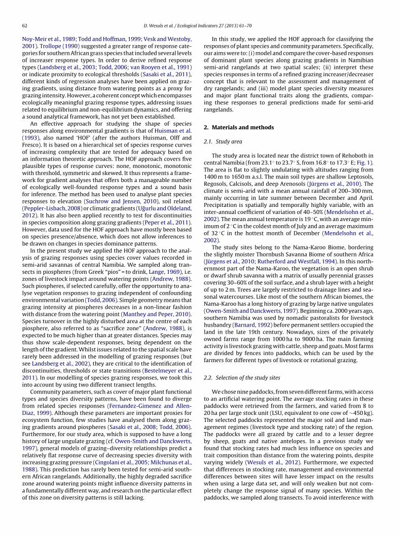
The study area is located near the district town of Rehoboth incentral Namibia (from 23.1◦ to 23.7◦ S, from 16.8◦ to 17.3◦ E; Fig. 1).The area is flat to slightly undulating with altitudes ranging from1400 m to 1650 m a.s.l. The main soil types are shallow Leptosols,Regosols, Calcisols, and deep Arenosols (Jürgens et al., 2010). Theclimate is semi-arid with a mean annual rainfall of 200–300 mm,mainly occurring in late summer between December and April.Precipitation is spatially and temporally highly variable, with aninter-annual coefficient of variation of 40–50% (Mendelsohn et al.,2002). The mean annual temperature is 19 ◦C, with an average min-imum of 2 ◦C in the coldest month of July and an average maximumof 32 ◦C in the hottest month of December (Mendelsohn et al.,2002).
The study sites belong to the Nama-Karoo Biome, borderingthe slightly moister Thornbush Savanna Biome of southern Africa(Jürgens et al., 2010; Rutherford and Westfall, 1994). In this north-ernmost part of the Nama-Karoo, the vegetation is an open shrubor dwarf shrub savanna with a matrix of usually perennial grassescovering 30–60% of the soil surface, and a shrub layer with a heightof up to 2 m. Trees are largely restricted to drainage lines and sea-sonal watercourses. Like most of the southern African biomes, theNama-Karoo has a long history of grazing by large native ungulates(Owen-Smith and Danckwerts, 1997). Beginning ca. 2000 years ago,southern Namibia was used by nomadic pastoralists for livestockhusbandry (Barnard, 1992) before permanent settlers occupied theland in the late 19th century. Nowadays, sizes of the privatelyowned farms range from 1000 ha to 9000 ha. The main farmingactivity is livestock grazing with cattle, sheep and goats. Most farmsare divided by fences into paddocks, which can be used by thefarmers for different types of livestock or rotational grazing.
2.2. Selection of the study sites
We chose nine paddocks, from seven different farms, with accessto an artificial watering point. The average stocking rates in thesepaddocks were retrieved from the farmers, and varied from 8 to20 ha per large stock unit (LSU, equivalent to one cow of ∼450 kg).The selected paddocks represented the major soil and land man-agement regimes (livestock type and stocking rate) of the region.The paddocks were all grazed by cattle and to a lesser degreeby sheep, goats and native antelopes. In a previous study wefound that stocking rates had much less influence on species andtrait composition than distance from the watering points, despitevarying widely (Wesuls et al., 2012). Furthermore, we expectedthat differences in stocking rate, management and environmental
differences between sites will have lesser impact on the resultswhen using a large data set, and will only weaken but not com-pletely change the response signal of many species. Within thepaddocks, we sampled along transects. To avoid interference with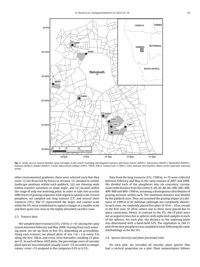
D. Wesuls et al. / Ecological Indicators 27 (2013) 61–70 63
Rehoboth
TSW2
TSW1
TSK1 TJW1
NAW1
MAW1
KOW2
KAW2
DUW1
17°30'E17°20'E17°10'E17°0'E16°50'E
23°0'S
23°10'S
23°20'S
23°30'S
23°40'S
23°50'S 0 10 205
Kilometers
NAMIBIA
ANGOLA
SOUTH AFRICA
BOTSWAN A
ZAMBIA
F stigatK 1); Tsp
owlwtdptwa
2
siAappv
ig. 1. Study area in central Namibia (grey rectangle in the insert) including inveamasis (KAW2); Kojeka (KOW2); Tsumis Agricultural College (TSW1, TSW2, TSKoints.
ther environmental gradients, these were selected such that theyere: (i) not dissected by fences or streams; (ii) situated in similar
andscape positions within each paddock; (iii) not showing wideithin-transect variations in slope angle; and (iv) located within
he range of only one watering point. In order to take into accountifferences of grazing responses with regard to spatial scale, in eachiosphere, we sampled one long transect (LT) and several shortransects (STs). The LT represented the larger and coarser scalehile the STs were established to capture changes at a smaller scale
nd finer grain size close to the highly disturbed sacrifice zone.
.3. Transect data
We sampled short transects (STs; 150 m; n = 41) during the rainyeason between February and May 2008. Starting from each water-ng point, we set up three to five STs, depending on accessibility.long each transect, we placed plots of size 1 m × 1 m every 5 m
long the first 100 m, and every 10 m thereafter, totalling 25 plotser ST. In each of these 1025 plots, the percentage cover of vascularlant species was estimated visually (cover >1% recorded as integeralues; cover <1% assigned to the categories 0.5% or 0.1%).ed transects and farms Narais (NAW1); Duruchaus (DUW1); Marienhof (MAW1);umis Ged. 5 (TJW1). Lines indicate farm borders. Black circles represent watering
Data from the long transects (LTs; 1500 m; n = 9) were collectedbetween February and May in the rainy seasons of 2007 and 2008.We divided each of the piospheres into six concentric circularzones with distance from the centre 0–20, 20–80, 80–200, 200–400,400–800 and 800–1500 m, assuming a homogenous distribution ofgrazing pressure within each. The maximum distance was limitedby the paddock sizes. Thus, we assumed the grazing impact at a dis-tance of 1500 m to be minimal (although not completely absent).In each zone, we randomly placed five plots of 10 m × 10 m, exceptin the first zone (0–20 m) where one to three were placed due tospace constraints. Hence, in contrast to the STs, the LT plots werenot arranged in lines but in spheres with replicated samples in eachof the spheres. For each plot, the distance to the watering pointwas determined with a hand-held GPS. The vegetation in 244 LTplots from nine piospheres was sampled in total, following the samemethodology as for the STs.
2.4. Species diversity and plant functional traits
On each plot, we recorded all vascular plant species thathad a vertical projection on a plot. Plant nomenclature follows
6 al Ind
GsTcrvgno
2
admigPtgcdepfio
mtmmrirmubndliA
eweifswumcsfhr
3
dg
4 D. Wesuls et al. / Ecologic
ermishuizen and Meyer (2003). For each plot, we calculatedpecies richness and Simpson diversity index (Magurran, 2004).he latter reflects the equitability in species cover and thereforeovers another aspect of species diversity. For each species, weecorded two traits: life cycle (annual, weak perennial – i.e., sur-ival depending on environmental conditions – or perennial) androwth form (grass/sedge, herbaceous forb, woody forb – i.e. peren-ial or weak perennial forbs with woody stem base, dwarf shrub,r shrub/tree). See Appendix C for species occurrences and traits.
.5. Modelling of grazing responses
As a proxy parameter for grazing intensity and predictor vari-ble for the modelling of grazing responses, we used the inverseistance (in m−1) from the watering point. In comparison with nor-al distance, which is usually used for the modelling of piospheres,
nverse distance better represents the non-linear distribution ofrazing pressure around circular grazing gradients (Manthey andeper, 2010). Furthermore, the interpretation is straightforward inhe sense that high values of inverse distance imply high levels ofrazing intensity. The use of this metric is based on the fact that aircular area impacted by livestock becomes larger with increasingistance. Under the simplifying assumption that livestock pres-nce is evenly distributed in relation to distance from the wateringoint, this means that animal density decreases in a non-linearashion. By using inverse distance, the study of grazing responsess less confounded by spatial piosphere patterns, e.g. non-linearityr thresholds emerging close to the sacrifice zone.
The grazing responses of single species, as well as diversityeasures and selected plant functional traits, were modelled using
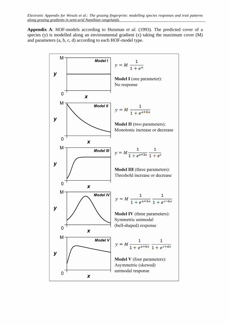
he HOF approach (Huisman et al., 1993). This method selects theinimum adequate model out of a set of five increasingly complexodels that correspond to typical responses of species to envi-
onmental gradients (Appendix A, see also Appendix D). Model Indicates no change along a gradient, whereas models II–V cor-espond to the following responses: (II) monotone sigmoid; (III)onotone sigmoid with plateau (i.e. threshold); (IV) symmetric
nimodal; and (V) skewed unimodal. We based the selection of theest model on the Akaike information criterion, corrected for small
(AICc; Burnham and Anderson, 2002). For model comparison, weetermined Akaike weights (wi), representing “normalised relative
ikelihoods” that sum up to 1, giving the probability that model is the best among the set of alternatives considered (Burnham andnderson, 2002).
For the unimodal responses (models IV and V), we calculatedach species’ optimum, i.e. the distance from the watering pointith the highest predicted cover. We restricted the HOF mod-
lling to species with at least 40 occurrences (3.9% frequency)n the 1025 ST plots and a minimum of ten occurrences (4.1%requency) in the 244 LT plots. If two or more models for onepecies were ascribed the same value of wi, we chose the oneith the fewest parameters as the best possible. For model eval-ation, we considered both the respective best model, and allodels with wi ≥ 0.01. For modelling a life cycle or growth form
ategory, we summed up the cover values of the respectivepecies. The modelling and calculation of species optima were per-ormed using the vegdata.dev package (Jansen, 2008; version 0.2.1,ttp://geobot.botanik.uni-greifswald.de/download) in the R envi-onment (R Development Core Team, 2011).
. Results
Some 162 species occurred in the 1025 ST plots, with a meanensity of 8 species per 1 m2 (range: 1–18). The annual grass Era-rostis porosa was most frequent (72%). In the 244 LT plots, 208
icators 27 (2013) 61–70
species occurred, with a mean density of 18 species per 100 m2
(range: 3–32). Here, the perennial grass Stipagrostis uniplumis wasmost frequent (82%). Combining both transect types, we found 225species, with 145 being common (see also Appendix C).
3.1. Species response curves
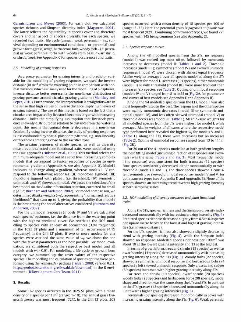
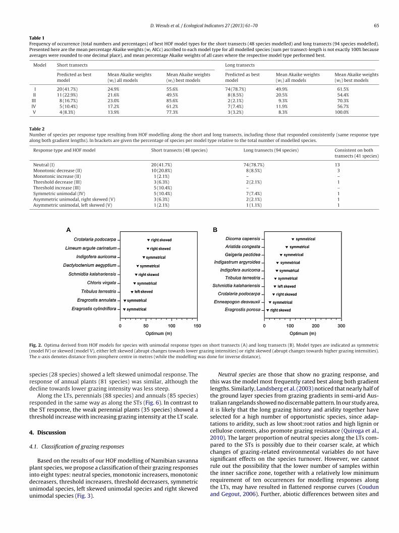
Among the 48 modelled species from the STs, no response(model I) was ranked top most often, followed by monotonicincreases or decreases (model II; Tables 1 and 2). Thresholdincreases (model III); symmetric (model IV) and skewed unimodalresponses (model V) were chosen with almost equal frequency.Akaike weights averaged over all species modelled along the STswere highest for model I. Decreases (13 species), either monotonic(model II) or with threshold (model III), were more frequent thanincreases (six species, see Table 2). Optima of unimodal responses(models IV and V) ranged from 8 m to 55 m (Fig. 2A, for parametersand curves of best models see Appendix E and Appendix B).
Among the 94 modelled species from the LTs, model I was alsomost frequently rated as the best. The responses of the other specieswere mainly monotonic decreases (model II) or symmetric uni-modal (model IV), and less often skewed unimodal (model V) orthreshold decreases (model III; Table 1). Mean Akaike weights forall modelled species from the LTs were highest for model I, whileaveraged Akaike weights of all cases where the respective modeltype performed best revealed the highest wi for models V and III(Table 1). Along the LTs, there were decreases but no increases(Table 2). Optima of unimodal responses ranged from 13 to 111 m(Fig. 2B).
For 20 out of the 41 species modelled at both gradient lengths,the best fitting model (including direction of responses and skew-ness) was the same (Table 2 and Fig. 3). Most frequently, modelI (no response) was consistent for both transects (13 species).Four species consistently decreased, either monotonically or withthreshold (models II and III), and three species showed a consis-tent symmetric or skewed unimodal response (model IV and V) forboth transect types (see Appendix D and Appendix B). None of thespecies showed an increasing trend towards high grazing intensityat both sampling scales.
3.2. HOF-modelling of diversity measures and plant functionaltraits
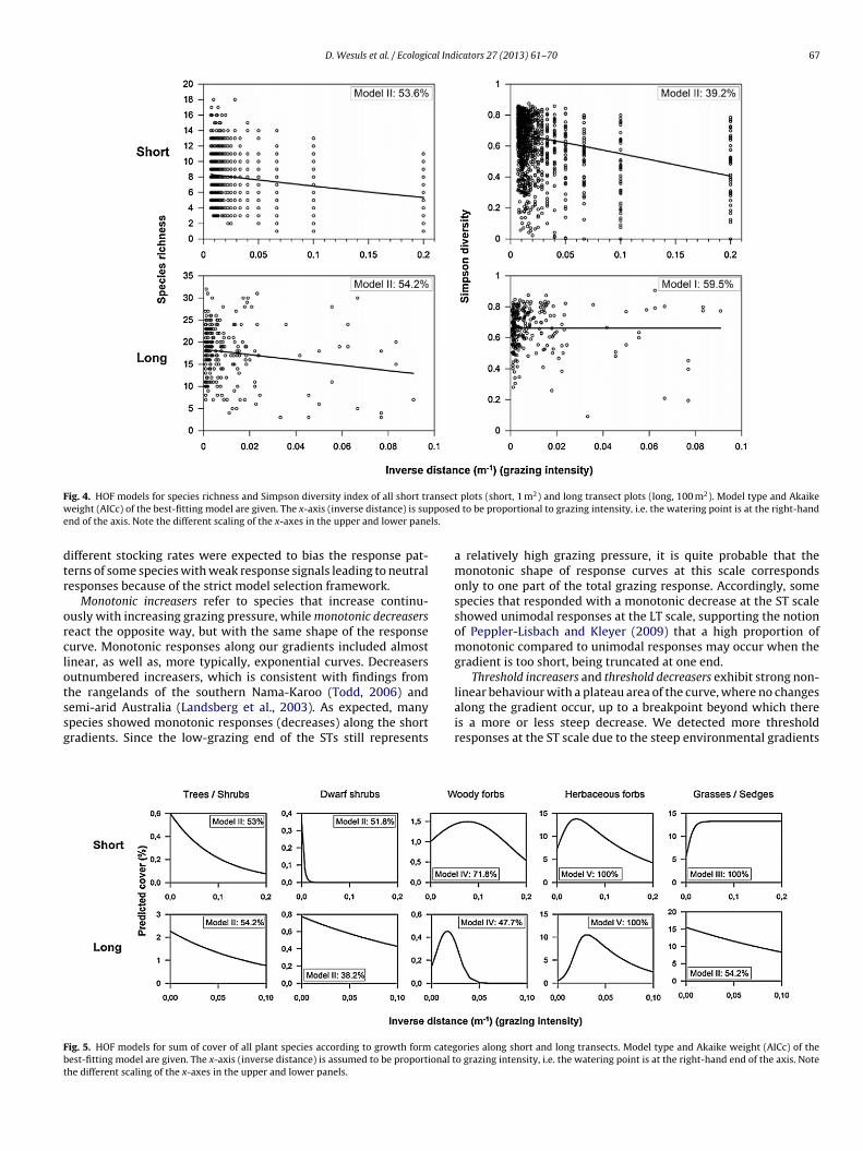
Along the STs, species richness and the Simpson diversity indexdecreased monotonically with increasing grazing intensity (Fig. 4).Predicted species richness decreased slightly from 8.5 to 6.0 speciesper square metre between the lowest and highest grazing intensi-ties (i.e. inverse distance).
For the LTs, species richness also showed a slightly decreasingtrend with grazing intensity (Fig. 4), while the Simpson indexshowed no response. Modelled species richness per 100 m2 wasabout 18 at the lowest grazing intensity and 13 at the highest.
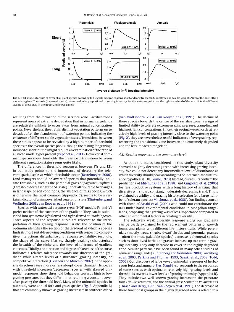
In terms of growth form, trees and shrubs (13 species) as well asdwarf shrubs (14 species) decreased monotonically with increasinggrazing intensity along the STs (Fig. 5). Woody forbs (22 species)showed a symmetric unimodal response and herbaceous forbs (74species) a left skewed unimodal response. Only grasses and sedges(39 species) increased with higher grazing intensity along STs.
For trees and shrubs (19 species), dwarf shrubs (20 species),woody forbs (28 species) and herbaceous forbs (98 species), modelshape and direction was the same along the LTs and STs. In contrast
to the STs, grasses (43 species) decreased monotonically along theLTs towards higher grazing intensities (Fig. 5).Perennials (53 species) decreased monotonically in cover withincreasing grazing intensity along the STs (Fig. 6). Weak perennial
D. Wesuls et al. / Ecological Indicators 27 (2013) 61–70 65
Table 1Frequency of occurrence (total numbers and percentages) of best HOF model types for the short transects (48 species modelled) and long transects (94 species modelled).Presented here are the mean percentage Akaike weights (wi AICc) ascribed to each model type for all modelled species (sum per transect-length is not exactly 100% becauseaverages were rounded to one decimal place), and mean percentage Akaike weights of all cases where the respective model type performed best.
Model Short transects Long transects
Predicted as bestmodel
Mean Akaike weights(wi) all models
Mean Akaike weights(wi) best models
Predicted as bestmodel
Mean Akaike weights(wi) all models
Mean Akaike weights(wi) best models
I 20 (41.7%) 24.9% 55.6% 74 (78.7%) 49.9% 61.5%II 11 (22.9%) 21.6% 49.5% 8 (8.5%) 20.5% 54.4%
III 8 (16.7%) 23.0% 85.6% 2 (2.1%) 9.3% 70.3%IV 5 (10.4%) 17.2% 61.2% 7 (7.4%) 11.9% 56.7%V 4 (8.3%) 13.9% 77.3% 3 (3.2%) 8.3% 100.0%
Table 2Number of species per response type resulting from HOF modelling along the short and long transects, including those that responded consistently (same response typealong both gradient lengths). In brackets are given the percentage of species per model type relative to the total number of modelled species.
Response type and HOF model Short transects (48 species) Long transects (94 species) Consistent on bothtransects (41 species)
Neutral (I) 20 (41.7%) 74 (78.7%) 13Monotonic decrease (II) 10 (20.8%) 8 (8.5%) 3Monotonic increase (II) 1 (2.1%) – –Threshold decrease (III) 3 (6.3%) 2 (2.1%) 1Threshold increase (III) 5 (10.4%) – –Symmetric unimodal (IV) 5 (10.4%) 7 (7.4%) 1Asymmetric unimodal, right skewed (V) 3 (6.3%) 2 (2.1%) 1Asymmetric unimodal, left skewed (V) 1 (2.1%) 1 (1.1%) 1
F s on s( grazinT as do
srd
rtt
4
4
piduu
ig. 2. Optima derived from HOF models for species with unimodal response typemodel IV) or skewed (model V), either left skewed (abrupt changes towards lower
he x-axis denotes distance from piosphere centre in metres (while the modelling w
pecies (28 species) showed a left skewed unimodal response. Theesponse of annual plants (81 species) was similar, although theecline towards lower grazing intensity was less steep.
Along the LTs, perennials (88 species) and annuals (85 species)esponded in the same way as along the STs (Fig. 6). In contrast tohe ST response, the weak perennial plants (35 species) showed ahreshold increase with increasing grazing intensity at the LT scale.
. Discussion
.1. Classification of grazing responses
Based on the results of our HOF modelling of Namibian savannalant species, we propose a classification of their grazing responses
nto eight types: neutral species, monotonic increasers, monotonicecreasers, threshold increasers, threshold decreasers, symmetricnimodal species, left skewed unimodal species and right skewednimodal species (Fig. 3).
hort transects (A) and long transects (B). Model types are indicated as symmetricg intensities) or right skewed (abrupt changes towards higher grazing intensities).ne for inverse distance).
Neutral species are those that show no grazing response, andthis was the model most frequently rated best along both gradientlengths. Similarly, Landsberg et al. (2003) noticed that nearly half ofthe ground layer species from grazing gradients in semi-arid Aus-tralian rangelands showed no discernable pattern. In our study area,it is likely that the long grazing history and aridity together haveselected for a high number of opportunistic species, since adap-tations to aridity, such as low shoot:root ratios and high lignin orcellulose contents, also promote grazing resistance (Quiroga et al.,2010). The larger proportion of neutral species along the LTs com-pared to the STs is possibly due to their coarser scale, at whichchanges of grazing-related environmental variables do not havesignificant effects on the species turnover. However, we cannotrule out the possibility that the lower number of samples within
the inner sacrifice zone, together with a relatively low minimumrequirement of ten occurrences for modelling responses alongthe LTs, may have resulted in flattened response curves (Coudunand Gegout, 2006). Further, abiotic differences between sites and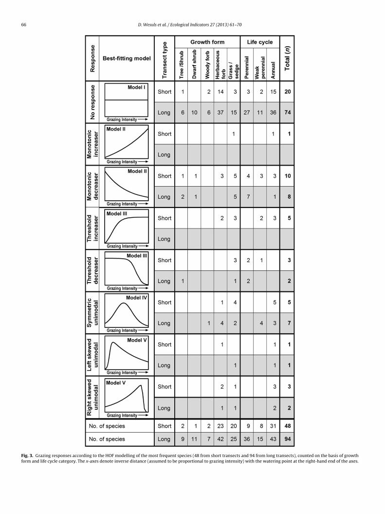
66 D. Wesuls et al. / Ecological Indicators 27 (2013) 61–70
Fig. 3. Grazing responses according to the HOF modelling of the most frequent species (48 from short transects and 94 from long transects), counted on the basis of growthform and life cycle category. The x-axes denote inverse distance (assumed to be proportional to grazing intensity) with the watering point at the right-hand end of the axes.
D. Wesuls et al. / Ecological Indicators 27 (2013) 61–70 67
F ansectw posee ls.
dtr
orclotssg
Fbt
ig. 4. HOF models for species richness and Simpson diversity index of all short treight (AICc) of the best-fitting model are given. The x-axis (inverse distance) is sup
nd of the axis. Note the different scaling of the x-axes in the upper and lower pane
ifferent stocking rates were expected to bias the response pat-erns of some species with weak response signals leading to neutralesponses because of the strict model selection framework.
Monotonic increasers refer to species that increase continu-usly with increasing grazing pressure, while monotonic decreaserseact the opposite way, but with the same shape of the responseurve. Monotonic responses along our gradients included almostinear, as well as, more typically, exponential curves. Decreasersutnumbered increasers, which is consistent with findings fromhe rangelands of the southern Nama-Karoo (Todd, 2006) and
emi-arid Australia (Landsberg et al., 2003). As expected, manypecies showed monotonic responses (decreases) along the shortradients. Since the low-grazing end of the STs still representsig. 5. HOF models for sum of cover of all plant species according to growth form categest-fitting model are given. The x-axis (inverse distance) is assumed to be proportional the different scaling of the x-axes in the upper and lower panels.
plots (short, 1 m2) and long transect plots (long, 100 m2). Model type and Akaiked to be proportional to grazing intensity, i.e. the watering point is at the right-hand
a relatively high grazing pressure, it is quite probable that themonotonic shape of response curves at this scale correspondsonly to one part of the total grazing response. Accordingly, somespecies that responded with a monotonic decrease at the ST scaleshowed unimodal responses at the LT scale, supporting the notionof Peppler-Lisbach and Kleyer (2009) that a high proportion ofmonotonic compared to unimodal responses may occur when thegradient is too short, being truncated at one end.
Threshold increasers and threshold decreasers exhibit strong non-linear behaviour with a plateau area of the curve, where no changes
along the gradient occur, up to a breakpoint beyond which thereis a more or less steep decrease. We detected more thresholdresponses at the ST scale due to the steep environmental gradientsories along short and long transects. Model type and Akaike weight (AICc) of theo grazing intensity, i.e. the watering point is at the right-hand end of the axis. Note
68 D. Wesuls et al. / Ecological Indicators 27 (2013) 61–70
Fig. 6. HOF models for sum of cover of all plant species according to life cycle categories along short and long transects. Model type and Akaike weight (AICc) of the best-fittingm ing ints
rrapdetsiaid
ivLc(iitV
pvTpofiitteidcswmgaot
odel are given. The x-axis (inverse distance) is assumed to be proportional to grazcaling of the x-axes in the upper and lower panels.
esulting from the formation of the sacrifice zone. Sacrifice zonesepresent areas of extreme degradation that in normal rangelandsre relatively unlikely to occur away from animal concentrationoints. Nevertheless, they retain distinct vegetation patterns up toecades after the abandonment of watering points, indicating thexistence of different stable vegetation states. Transitions betweenhese states appear to be revealed by a high number of thresholdpecies in the overall species pool, although the testing for grazing-nduced discontinuities might require an examination of the ratio ofll niche model types present (Peper et al., 2011). However, if dom-nant species show thresholds, the presence of transitions betweenifferent vegetation states seems quite likely.
The differences in threshold responses between STs and LTsn our study points to the importance of detecting the rele-ant spatial scale at which thresholds occur (Bestelmeyer, 2006).and managers should be aware of species that potentially indi-ate thresholds, such as the perennial grass Stipagrostis uniplumisthreshold decreaser at the ST scale). If not attributable to changesn landscape or soil conditions, the absence of this species, whichs otherwise the most common (Appendix C), seems to be a cer-ain indicator of an impoverished vegetation state (Klintenberg anderlinden, 2008; van Rooyen et al., 1991).
Species with unimodal response types (HOF models IV and V)refer neither of the extremes of the gradient. They can be subdi-ided into symmetric, left skewed and right skewed unimodal species.hree aspects of the response curve are relevant to the inter-retation of their grazing response. Firstly, the position of theptimum identifies the section of the gradient at which a speciesnds its most suitable growing conditions with respect to compet-
tive interactions, disturbance and resource availability. Secondly,he shape of the curve (flat vs. sharply peaking) characteriseshe breadth of the niche and the level of tolerance of gradientxtremes. Thirdly, the direction and degree of skewness of the curvendicates a relative tolerance towards one direction of the gra-ient, while altered levels of disturbance (grazing intensity) orompetitive interaction (Oksanen and Minchin, 2002) in the oppo-ite direction cause more or less abrupt cover changes. Hence, asith threshold increasers/decreasers, species with skewed uni-odal responses show threshold behaviour towards high or low
razing pressure, but they differ in not retaining a constant coverfter passing the threshold level. Many of the unimodal species inur study were annual forb and grass species (Fig. 3, Appendix B)hat are commonly known as grazing increasers in southern Africa
ensity, i.e. the watering point is at the right-hand end of the axis. Note the different
(van Oudtshoorn, 2004; van Rooyen et al., 1991). The decline ofthese species towards the centre of the sacrifice zone is a sign oflimited ability to tolerate extreme grazing pressure, trampling andhigh nutrient concentrations. Since their optima were mostly at rel-atively high levels of grazing intensity close to the watering point(Fig. 2), they are nevertheless useful indicators of overgrazing, rep-resenting the transitional zone between the extremely degradedand the less impacted rangeland.
4.2. Grazing responses at the community level
At both the scales considered in this study, plant diversityshowed a slightly decreasing trend with increasing grazing inten-sity. We could not detect any intermediate level of disturbance atwhich diversity should peak according to the intermediate disturb-ance hypothesis (IDH, Grime, 1973). Instead, our results confirm thepredictions of Milchunas et al. (1988) and Cingolani et al. (2005)for less productive systems with a long history of grazing, thatdiversity will show a constant, moderately decreasing trend. This isexplained by aridity and grazing history selecting for a large num-ber of tolerant species (Milchunas et al., 1988). Our findings concurwith those of Sasaki et al. (2009) who could not corroborate theIDH under harsh environmental conditions in Mongolian range-lands, proposing that grazing was of less importance compared toother environmental factors in creating diversity.
The relatively weak diversity response along our gradientscan be partly explained by the replacement patterns of growthforms and plants with different life history traits. While peren-nials (mostly trees, shrubs, dwarf shrubs and perennial grasses– often the most palatable species) decrease, ephemeral speciessuch as short-lived herbs and grasses increase up to a certain graz-ing intensity. They only decrease in cover in the highly degradedzone. Similar patterns have been found in many other studies ofsemi-arid rangelands (Klintenberg and Verlinden, 2008; Landsberget al., 2003; Perkins and Thomas, 1993; Sasaki et al., 2008; Todd,2006). Our discovery of left-skewed unimodal responses of herba-ceous forbs and annuals (Figs. 5 and 6) corresponds to the responsesof some species with optima at relatively high grazing levels andthresholds towards lower levels of grazing intensity (Appendix B).
They include two well-known grazing increasers: the prostrateforb Tribulus terrestris, and the annual grass Schmidtia kalahariensis(Thrash and Derry, 1999; van Rooyen et al., 1991). The decrease ofthese functional groups in the highly degraded zone is related to a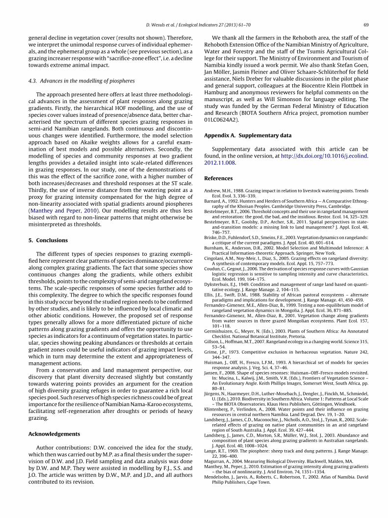
al Ind
gwagt
4
cgsasuaimlitbTpn(bm
5
fiactttibotpsugwm
dtosifg
A
wvbJc
D. Wesuls et al. / Ecologic
eneral decline in vegetation cover (results not shown). Therefore,e interpret the unimodal response curves of individual ephemer-
ls, and the ephemeral group as a whole (see previous section), as arazing increaser response with “sacrifice-zone effect”, i.e. a declineowards extreme animal impact.
.3. Advances in the modelling of piospheres
The approach presented here offers at least three methodologi-al advances in the assessment of plant responses along grazingradients. Firstly, the hierarchical HOF modelling, and the use ofpecies cover values instead of presence/absence data, better char-cterised the spectrum of different species grazing responses inemi-arid Namibian rangelands. Both continuous and discontin-ous changes were identified. Furthermore, the model selectionpproach based on Akaike weights allows for a careful exam-nation of best models and possible alternatives. Secondly, the
odelling of species and community responses at two gradientengths provides a detailed insight into scale-related differencesn grazing responses. In our study, one of the demonstrations ofhis was the effect of the sacrifice zone, with a higher number ofoth increases/decreases and threshold responses at the ST scale.hirdly, the use of inverse distance from the watering point as aroxy for grazing intensity compensated for the high degree ofon-linearity associated with spatial gradients around piospheresManthey and Peper, 2010). Our modelling results are thus lessiased with regard to non-linear patterns that might otherwise beisinterpreted as thresholds.
. Conclusions
The different types of species responses to grazing exempli-ed here represent clear patterns of species dominance/occurrencelong complex grazing gradients. The fact that some species showontinuous changes along the gradients, while others exhibithresholds, points to the complexity of semi-arid rangeland ecosys-ems. The scale-specific responses of some species further add tohis complexity. The degree to which the specific responses foundn this study occur beyond the studied region needs to be confirmedy other studies, and is likely to be influenced by local climatic andther abiotic conditions. However, the proposed set of responseypes generally allows for a more differentiated picture of nicheatterns along grazing gradients and offers the opportunity to usepecies as indicators for a continuum of vegetation states. In partic-lar, species showing peaking abundances or thresholds at certainradient zones could be useful indicators of grazing impact levels,hich in turn may determine the extent and appropriateness ofanagement actions.From a conservation and land management perspective, our
iscovery that plant diversity decreased slightly but constantlyowards watering points provides an argument for the creationf high diversity grazing refuges in order to guarantee a rich localpecies pool. Such reserves of high species richness could be of greatmportance for the resilience of Namibian Nama-Karoo ecosystems,acilitating self-regeneration after droughts or periods of heavyrazing.
cknowledgements
Author contributions: D.W. conceived the idea for the study,hich then was carried out by M.P. as a final thesis under the super-
ision of D.W. and J.D. Field sampling and data analysis was doney D.W. and M.P. They were assisted in modelling by F.J., S.S. and.O. The article was written by D.W., M.P. and J.D., and all authorsontributed to its revision.
icators 27 (2013) 61–70 69
We thank all the farmers in the Rehoboth area, the staff of theRehoboth Extension Office of the Namibian Ministry of Agriculture,Water and Forestry and the staff of the Tsumis Agricultural Col-lege for their support. The Ministry of Environment and Tourism ofNamibia kindly issued a work permit. We also thank Stefan Goen,Jan Möller, Jasmin Fleiner and Oliver Schaare-Schlüterhof for fieldassistance, Niels Dreber for valuable discussions in the pilot phaseand general support, colleagues at the Biocentre Klein Flottbek inHamburg and anonymous reviewers for helpful comments on themanuscript, as well as Will Simonson for language editing. Thestudy was funded by the German Federal Ministry of Educationand Research (BIOTA Southern Africa project, promotion number01LC0624A2).
Appendix A. Supplementary data
Supplementary data associated with this article can befound, in the online version, at http://dx.doi.org/10.1016/j.ecolind.2012.11.008.
References
Andrew, M.H., 1988. Grazing impact in relation to livestock watering points. TrendsEcol. Evol. 3, 336–339.
Barnard, A., 1992. Hunters and Herders of Southern Africa — A Comparative Ethnog-raphy of the Khoisan Peoples. Cambridge University Press, Cambridge.
Bestelmeyer, B.T., 2006. Threshold concepts and their use in rangeland managementand restoration: the good, the bad, and the insidious. Restor. Ecol. 14, 325–329.
Bestelmeyer, B.T., Goolsby, D.P., Archer, S.R., 2011. Spatial perspectives in state-and-transition models: a missing link to land management? J. Appl. Ecol. 48,746–757.
Briske, D.D., Fuhlendorf, S.D., Smeins, F.E., 2003. Vegetation dynamics on rangelands:a critique of the current paradigms. J. Appl. Ecol. 40, 601–614.
Burnham, K., Anderson, D.R., 2002. Model Selection and Multimodel Inference: APractical Information-theoretic Approach. Springer, New York.
Cingolani, A.M., Noy-Meir, I., Diaz, S., 2005. Grazing effects on rangeland diversity:A synthesis of contemporary models. Ecol. Appl. 15, 757–773.
Coudun, C., Gegout, J., 2006. The derivation of species response curves with Gaussianlogistic regression is sensitive to sampling intensity and curve characteristics.Ecol. Model. 199, 164–175.
Dyksterhuis, E.J., 1949. Condition and management of range land based on quanti-tative ecology. J. Range Manage. 2, 104–115.
Ellis, J.E., Swift, D.M., 1988. Stability of African pastoral ecosystems – alternateparadigms and implications for development. J. Range Manage. 41, 450–459.
Fernandez-Gimenez, M.E., Allen-Diaz, B., 1999. Testing a non-equilibrium model ofrangeland vegetation dynamics in Mongolia. J. Appl. Ecol. 36, 871–885.
Fernandez-Gimenez, M., Allen-Diaz, B., 2001. Vegetation change along gradientsfrom water sources in three grazed Mongolian ecosystems. Plant Ecol. 157,101–118.
Germishuizen, G., Meyer, N. (Eds.), 2003. Plants of Southern Africa: An AnnotatedChecklist. National Botanical Institute, Pretoria.
Gillson, L., Hoffman, M.T., 2007. Rangeland ecology in a changing world. Science 315,53–54.
Grime, J.P., 1973. Competitive exclusion in herbaceous vegetation. Nature 242,344–347.
Huisman, J., Olff, H., Fresco, L.F.M., 1993. A hierarchical set of models for speciesresponse analysis. J. Veg. Sci. 4, 37–46.
Jansen, F., 2008. Shape of species resonses: Huisman–Olff–Fresco models revisited.In: Mucina, L., Kalwij, J.M., Smith, V.R. (Eds.), Frontiers of Vegetation Science –An Evolutionary Angle. Keith Phillips Images, Somerset West, South Africa, pp.80–81.
Jürgens, N., Haarmeyer, D.H., Luther-Mosebach, J., Dengler, J., Finckh, M., Schmiedel,U. (Eds.), 2010. Biodiversity in Southern Africa. Volume 1: Patterns at Local Scale– The BIOTA Observatories. Klaus Hess Publishers, Göttingen, Windhoek.
Klintenberg, P., Verlinden, A., 2008. Water points and their influence on grazingresources in central northern Namibia. Land Degrad. Dev. 19, 1–20.
Landsberg, J., James, C.D., Maconochie, J., Nicholls, A.O., Stol, J., Tynan, R., 2002. Scale-related effects of grazing on native plant communities in an arid rangelandregion of South Australia. J. Appl. Ecol. 39, 427–444.
Landsberg, J., James, C.D., Morton, S.R., Müller, W.J., Stol, J., 2003. Abundance andcomposition of plant species along grazing gradients in Australian rangelands.J. Appl. Ecol. 40, 1008–1024.
Lange, R.T., 1969. The piosphere: sheep track and dung patterns. J. Range Manage.22, 396–400.
Magurran, A., 2004. Measuring Biological Diversity. Blackwell, Malden, MA.Manthey, M., Peper, J., 2010. Estimation of grazing intensity along grazing gradients
– the bias of nonlinearity. J. Arid Environ. 74, 1351–1354.Mendelsohn, J., Jarvis, A., Roberts, C., Robertson, T., 2002. Atlas of Namibia. David
Philip Publishers, Cape Town.
7 al Ind
M
M
N
O
O
P
P
P
P
Q
R
R
S
Westoby, M., Walker, B., Noy-Meir, I., 1989. Opportunistic management for range-
0 D. Wesuls et al. / Ecologic
iehe, S., Kluge, J., Von Wehrden, H., Retzer, V., 2010. Long-term degradation ofSahelian rangeland detected by 27 years of field study in Senegal. J. Appl. Ecol.47, 692–700.
ilchunas, D.G., Sala, O.E., Lauenroth, W.K., 1988. A generalized model of the effectsof grazing by large herbivores on grassland community structure. Am. Nat. 132,87–106.
oy-Meir, I., Gutman, M., Kaplan, Y., 1989. Responses of Mediterranean grasslandplants to grazing and protection. J. Ecol. 77, 290–310.
ksanen, J., Minchin, P.R., 2002. Continuum theory revisited: what shape are speciesresponses along ecological gradients? Ecol. Model. 157, 119–129.
wen-Smith, N., Danckwerts, J.E., 1997. Herbivory. In: Cowling, R.M., Richardson,D.M., Pierce, S.M. (Eds.), Vegetation of Southern Africa. Cambridge UniversityPress, pp. 397–420.
eper, J., Jansen, F., Pietzsch, D., Manthey, M., 2011. Patterns of plant species turnoveralong grazing gradients. J. Veg. Sci. 22, 457–466.
eppler-Lisbach, C., 2008. Using species-environmental amplitudes to predict pHvalues from vegetation. J. Veg. Sci. 19, 437–444.
eppler-Lisbach, C., Kleyer, M., 2009. Patterns of species richness and turnover alongthe pH gradient in deciduous forests: testing the continuum hypothesis. J. Veg.Sci. 20, 984–995.
erkins, J.S., Thomas, D.S.G., 1993. Environmental responses and sensitivityto permanent cattle ranching semi-arid western Central Botswana. In:Thomas, D.S.G., Allison, R.J. (Eds.), Landscape Sensitivity. Wiley, Chichester,pp. 273–286.
uiroga, R.E., Golluscio, R.A., Blanco, L.J., Fernandez, R.J., 2010. Aridity and grazingas convergent selective forces: an experiment with an Arid Chaco bunchgrass.Ecol. Appl. 20, 1876–1889.
Development Core Team, 2011. R: A Language and Environment for Statistical
Computing. R Foundation for Statistical Computing, Vienna, Austria.utherford, M., Westfall, R.H., 1994. Biomes of Southern Africa: An Objective Cate-gorization. National Botanical Institute, Pretoria.
asaki, T., Okayasu, T., Jamsran, U., Takeuchi, K., 2008. Threshold changes in vegeta-tion along a grazing gradient in Mongolian rangelands. J. Ecol. 96, 145–154.
icators 27 (2013) 61–70
Sasaki, T., Okubo, S., Okayasu, T., Jamsran, U., Ohkuro, T., Takeuchi, K., 2009. Manage-ment applicability of the intermediate disturbance hypothesis across Mongolianrangeland ecosystems. Ecol. Appl. 19, 423–432.
Sasaki, T., Okubo, S., Okayasu, T., Jamsran, U., Ohkuro, T., Takeuchi, K., 2011. Indicatorspecies and functional groups as predictors of proximity to ecological thresholdsin Mongolian rangelands. Plant Ecol. 212, 327–342.
Suchrow, S., Jensen, K., 2010. Plant species responses to an elevational gradient inGerman North Sea salt marshes. Wetlands 30, 735–746.
Thrash, I., Derry, J.F., 1999. The nature and modelling of piospheres: a review. Koedoe42, 73–94.
Todd, S.W., 2006. Gradients in vegetation cover, structure and species richness ofNama-Karoo shrublands in relation to distance from livestock watering points.J. Appl. Ecol. 43, 293–304.
Todd, S.W., Hoffman, M.T., 1999. A fence-line contrast reveals effects of heavy graz-ing on plant diversity and community composition in Namaqualand, SouthAfrica. Plant Ecol. 142, 169–178.
Trollope, W.S.W., 1990. Development of a technique for assessing veld conditionin the Kruger National Park using key grass species. Journal of the GrasslandSociety of Southern Africa 7, 46–51.
Ugurlu, E., Oldeland, J., 2012. Species response curves of oak species along climaticgradients in Turkey. Int. J. Biometeorol. 56, 85–93.
van Oudtshoorn, F., 2004. Guide to Grasses of Southern Africa. Briza Publications,Pretoria South Africa.
van Rooyen, N., Bredenkamp, G.J., Theron, G.K., 1991. Kalahari vegetation: veld con-dition trends and ecological status of species. Koedoe 34, 61–72.
Vesk, P.A., Westoby, M., 2001. Predicting plant species’ responses to grazing. J. Appl.Ecol. 38, 897–909.
lands not at equilibrium. J. Range Manage. 42, 266–274.Wesuls, D., Oldeland, J., Dray, S., 2012. Disentangling plant trait responses to live-
stock grazing from spatio-temporal variation: the partial RLQ approach. J. Veg.Sci. 23, 98–113.
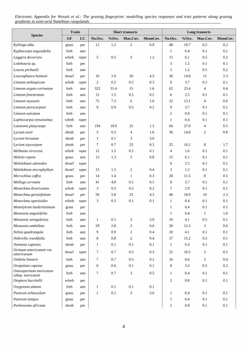
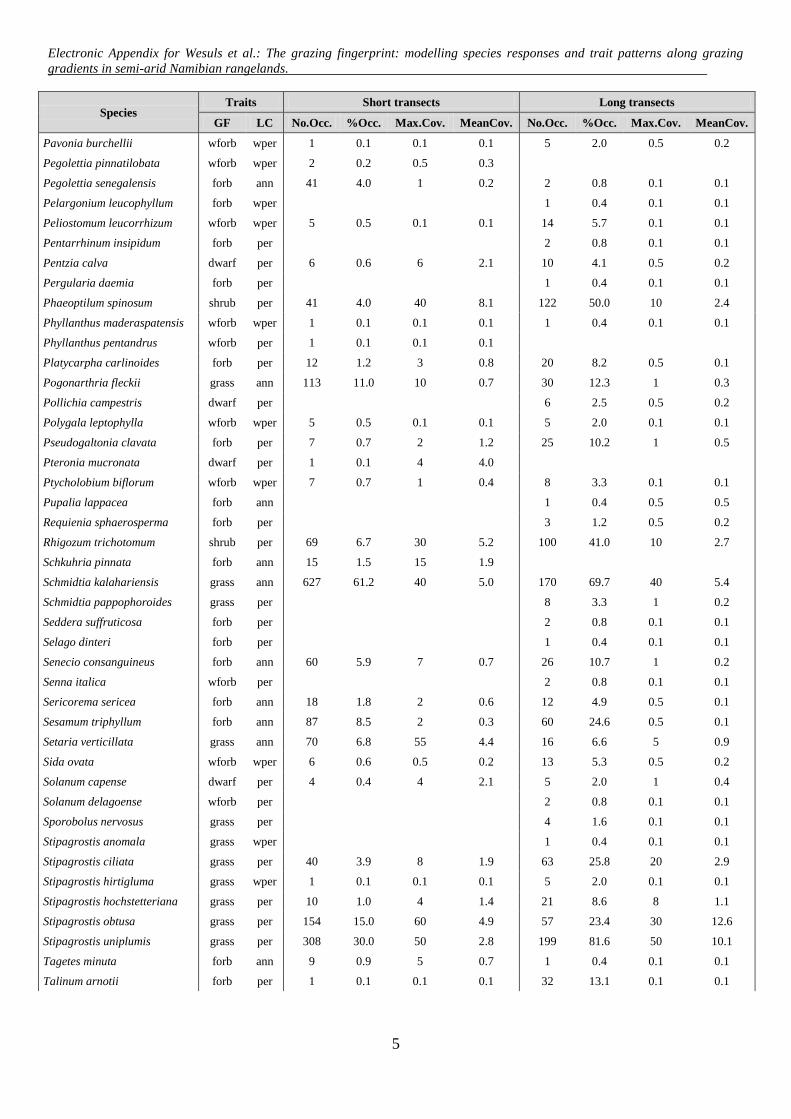
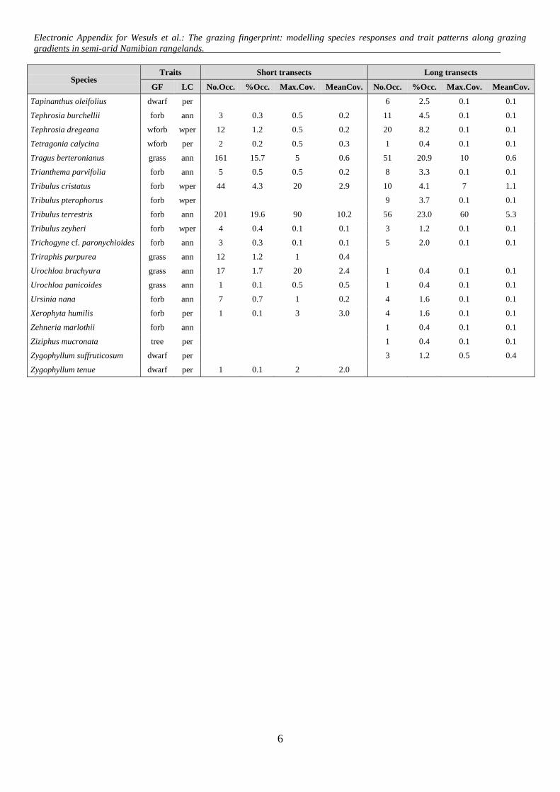
Electronic Appendix for Wesuls et al.: The grazing fingerprint: modelling species responses and trait patterns along grazing gradients in semi-arid Namibian rangelands.
Appendix A: HOF-models according to Huisman et al. (1993). The predicted cover of a species (y) is modelled along an environmental gradient (x) taking the maximum cover (M) and parameters (a, b, c, d) according to each HOF-model type.
Electronic Appendix for Wesuls et al.: The grazing fingerprint: modelling species responses and trait patterns
along grazing gradients in semi-arid Namibian rangelands.
1
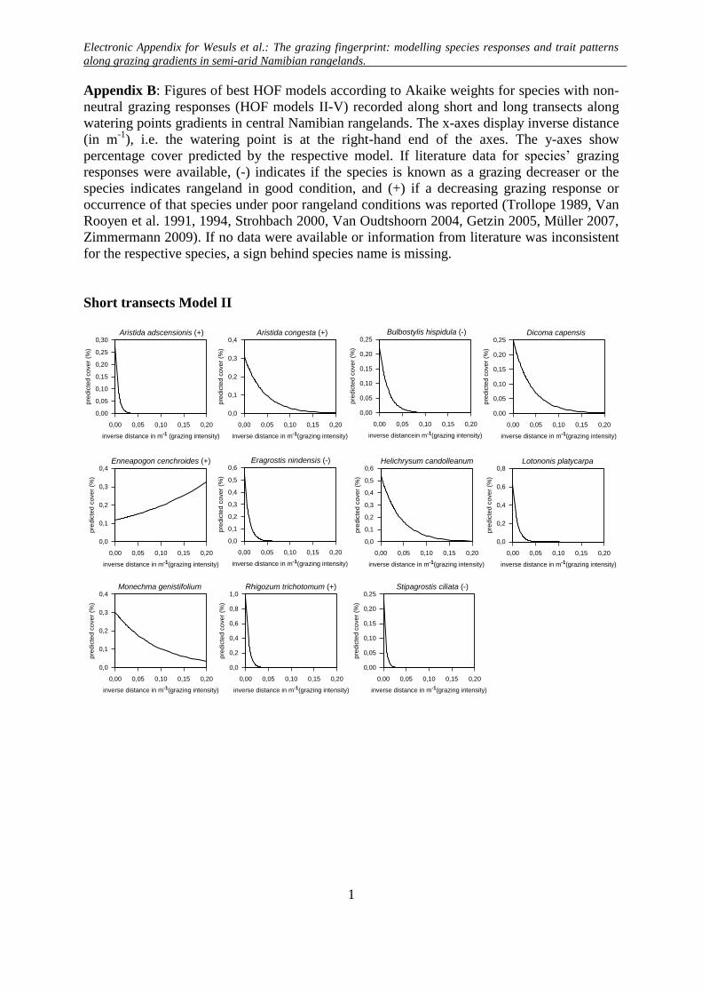
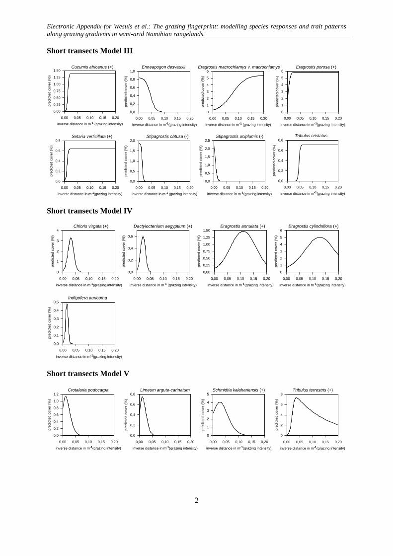
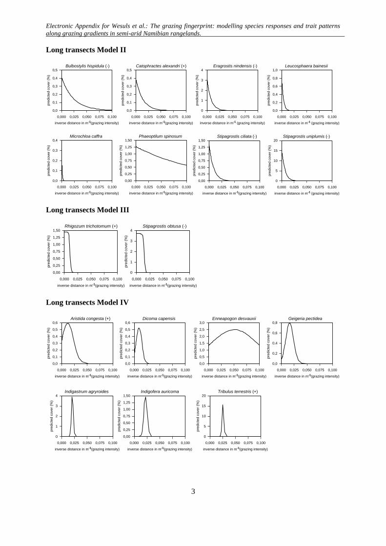
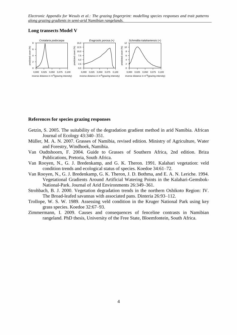
Appendix B: Figures of best HOF models according to Akaike weights for species with non-
neutral grazing responses (HOF models II-V) recorded along short and long transects along
watering points gradients in central Namibian rangelands. The x-axes display inverse distance
(in m-1
), i.e. the watering point is at the right-hand end of the axes. The y-axes show
percentage cover predicted by the respective model. If literature data for species’ grazing
responses were available, (-) indicates if the species is known as a grazing decreaser or the
species indicates rangeland in good condition, and (+) if a decreasing grazing response or
occurrence of that species under poor rangeland conditions was reported (Trollope 1989, Van
Rooyen et al. 1991, 1994, Strohbach 2000, Van Oudtshoorn 2004, Getzin 2005, Müller 2007,
Zimmermann 2009). If no data were available or information from literature was inconsistent
for the respective species, a sign behind species name is missing.
Short transects Model II
0,00
0,05
0,10
0,15
0,20
0,25
0,30
pre
dic
ted
cover
(%)
0,00 0,05 0,10 0,15 0,20
inverse distance in m (grazing intensity)-1
Aristida adscensionis (+)
0,0
0,1
0,2
0,3
0,4
pre
dic
ted
cover
(%)
0,00 0,05 0,10 0,15 0,20
inverse distance in m (grazing intensity)-1
Aristida congesta (+)
0,00
0,05
0,10
0,15
0,20
0,25
pre
dic
ted
cover
(%)
0,00 0,05 0,10 0,15 0,20
inverse distancein m (grazing intensity)-1
Bulbostylis hispidula (-)
0,00
0,05
0,10
0,15
0,20
0,25
pre
dic
ted
cover
(%)
0,00 0,05 0,10 0,15 0,20
inverse distance in m (grazing intensity)-1
Dicoma capensis
0,0
0,1
0,2
0,3
0,4
pre
dic
ted
cove
r(%
)
0,00 0,05 0,10 0,15 0,20
inverse distance in m (grazing intensity)-1
Enneapogon cenchroides (+)
0,0
0,1
0,2
0,3
0,4
0,5
0,6
pre
dic
ted
cover
(%)
0,00 0,05 0,10 0,15 0,20
inverse distance in m (grazing intensity)-1
Eragrostis nindensis (-)
0,0
0,1
0,2
0,3
0,4
0,5
0,6
pre
dic
ted
cove
r(%
)
0,00 0,05 0,10 0,15 0,20
inverse distance in m (grazing intensity)-1
Helichrysum candolleanum
0,0
0,2
0,4
0,6
0,8
pre
dic
ted
cove
r(%
)
0,00 0,05 0,10 0,15 0,20
inverse distance in m (grazing intensity)-1
Lotononis platycarpa
0,0
0,1
0,2
0,3
0,4
pre
dic
ted
co
ver
(%)
0,00 0,05 0,10 0,15 0,20
inverse distance in m (grazing intensity)-1
Monechma genistifolium
0,0
0,2
0,4
0,6
0,8
1,0
pre
dic
ted
co
ver
(%)
0,00 0,05 0,10 0,15 0,20
inverse distance in m (grazing intensity)-1
Rhigozum trichotomum (+)
0,00
0,05
0,10
0,15
0,20
0,25
pre
dic
ted
co
ver
(%)
0,00 0,05 0,10 0,15 0,20
inverse distance in m (grazing intensity)-1
Stipagrostis ciliata (-)
Electronic Appendix for Wesuls et al.: The grazing fingerprint: modelling species responses and trait patterns
along grazing gradients in semi-arid Namibian rangelands.
2
Short transects Model III
0,0
0,2
0,4
0,6
0,8
1,0
pre
dic
ted
cove
r(%
)
0,00 0,05 0,10 0,15 0,20
inverse distance in m (grazing intensity)-1
Enneapogon desvauxii
0
1
2
3
4
5
6
pre
dic
ted
cove
r(%
)
0,00 0,05 0,10 0,15 0,20
inverse distance in m (grazing intensity)-1
Eragrostis porosa (+)
0,0
0,2
0,4
0,6
0,8
pre
dic
ted
co
ver
(%)
0,00 0,05 0,10 0,15 0,20
inverse distance in m (grazing intensity)-1
Setaria verticillata (+)
0,0
0,5
1,0
1,5
2,0
2,5
pre
dic
ted
cove
r(%
)
0,00 0,05 0,10 0,15 0,20
inverse distance in m (grazing intensity)-1
Stipagrostis uniplumis (-)
0,0
0,2
0,4
0,6
0,8
pre
dic
ted
cover
(%)
0,00 0,05 0,10 0,15 0,20
inverse distance in m (grazing intensity)-1
Tribulus cristatus
0,00
0,25
0,50
0,75
1,00
1,25
1,50
pre
dic
ted
cover
(%)
0,00 0,05 0,10 0,15 0,20
inverse distance in m (grazing intensity)-1
Cucumis africanus (+)
0
1
2
3
4
5
6
pre
dic
ted
co
ver
(%)
0,00 0,05 0,10 0,15 0,20
inverse distance in m (grazing intensity)-1
Eragrostis macrochlamys v. macrochlamys
0,0
0,5
1,0
1,5
2,0
pre
dic
ted
co
ver
(%)
0,00 0,05 0,10 0,15 0,20
inverse distance in m (grazing intensity)-1
Stipagrostis obtusa (-)
Short transects Model IV
0
1
2
3
4
pre
dic
ted
co
ver
(%)
0,00 0,05 0,10 0,15 0,20
inverse distance in m (grazing intensity)-1
Chloris virgata (+)
0,00
0,25
0,50
0,75
1,00
1,25
1,50
pre
dic
ted
co
ver
(%)
0,00 0,05 0,10 0,15 0,20
inverse distance in m (grazing intensity)-1
Eragrostis annulata (+)
0
1
2
3
4
5
6
pre
dic
ted
co
ver
(%)
0,00 0,05 0,10 0,15 0,20
inverse distance in m (grazing intensity)-1
Eragrostis cylindriflora (+)
0,0
0,1
0,2
0,3
0,4
0,5
pre
dic
ted
cove
r(%
)
0,00 0,05 0,10 0,15 0,20
inverse distance in m (grazing intensity)-1
Indigofera auricoma
Dactyloctenium aegyptium (+)
0,0
0,2
0,4
0,6
pre
dic
ted
co
ver
(%)
0,00 0,05 0,10 0,15 0,20
inverse distance in m (grazing intensity)-1
Short transects Model V
0,0
0,2
0,4
0,6
0,8
1,0
1,2
pre
dic
ted
co
ver
(%)
0,00 0,05 0,10 0,15 0,20
inverse distance in m (grazing intensity)-1
Crotalaria podocarpa
0,0
0,2
0,4
0,6
0,8
pre
dic
ted
co
ver
(%)
0,00 0,05 0,10 0,15 0,20
inverse distance in m (grazing intensity)-1
Limeum argute-carinatum
0
1
2
3
4
5
pre
dic
ted
co
ver
(%)
0,00 0,05 0,10 0,15 0,20
inverse distance in m (grazing intensity)-1
Schmidtia kalahariensis (+)
0
2
4
6
8
pre
dic
ted
co
ver
(%)
0,00 0,05 0,10 0,15 0,20
inverse distance in m (grazing intensity)-1
Tribulus terrestris (+)
Electronic Appendix for Wesuls et al.: The grazing fingerprint: modelling species responses and trait patterns
along grazing gradients in semi-arid Namibian rangelands.
3
Long transects Model II
0,0
0,1
0,2
0,3
0,4
0,5
pre
dic
ted
co
ver
(%)
0,000 0,025 0,050 0,075 0,100
inverse distance in m (grazing intensity)-1
Bulbostylis hispidula (-)
0,0
0,1
0,2
0,3
0,4
0,5
pre
dic
ted
co
ver
(%)
0,000 0,025 0,050 0,075 0,100
inverse distance in m (grazing intensity)-1
Catophractes alexandri (+)
0,0
0,1
0,2
0,3
0,4
pre
dic
ted
cover
(%)
0,000 0,025 0,050 0,075 0,100
inverse distance in m (grazing intensity)-1
Microchloa caffra
0,00
0,25
0,50
0,75
1,00
1,25
1,50
pre
dic
ted
cove
r(%
)
0,000 0,025 0,050 0,075 0,100
inverse distance in m (grazing intensity)-1
Phaeoptilum spinosum
0,00
0,25
0,50
0,75
1,00
1,25
1,50
pre
dic
ted
co
ver
(%)
0,000 0,025 0,050 0,075 0,100
inverse distance in m (grazing intensity)-1
Stipagrostis ciliata (-)
0
1
2
3
4
pre
dic
ted
co
ver
(%)
0,000 0,025 0,050 0,075 0,100
inverse distance in m (grazing intensity)-1
Eragrostis nindensis (-)
0,0
0,2
0,4
0,6
0,8
1,0
pre
dic
ted
cove
r(%
)
0,000 0,025 0,050 0,075 0,100
inverse distance in m (grazing intensity)-1
Leucosphaera bainesii
0
5
10
15
20
pre
dic
ted
cove
r(%
)
0,000 0,025 0,050 0,075 0,100
inverse distance in m (grazing intensity)-1
Stipagrostis uniplumis (-)
Long transects Model III
0,00
0,25
0,50
0,75
1,00
1,25
1,50
pre
dic
ted
co
ver
(%)
0,000 0,025 0,050 0,075 0,100
inverse distance in m (grazing intensity)-1
Rhigozum trichotomum (+)
0
1
2
3
4
pre
dic
ted
co
ver
(%)
0,000 0,025 0,050 0,075 0,100
inverse distance in m (grazing intensity)-1
Stipagrostis obtusa (-)
Long transects Model IV
0,0
0,1
0,2
0,3
0,4
0,5
0,6
pre
dic
ted
co
ver
(%)
0,000 0,025 0,050 0,075 0,100
inverse distance in m (grazing intensity)-1
Aristida congesta (+)
0,0
0,1
0,2
0,3
0,4
0,5
0,6
pre
dic
ted
co
ver
(%)
0,000 0,025 0,050 0,075 0,100
inverse distance in m (grazing intensity)-1
Dicoma capensis
0,0
0,5
1,0
1,5
2,0
2,5
3,0
pre
dic
ted
co
ver
(%)
0,000 0,025 0,050 0,075 0,100
inverse distance in m (grazing intensity)-1
Enneapogon desvauxii
0,0
0,2
0,4
0,6
0,8
pre
dic
ted
co
ver
(%)
0,000 0,025 0,050 0,075 0,100
inverse distance in m (grazing intensity)-1
Geigeria pectidea
0
1
2
3
4
pre
dic
ted
cover
(%)
0,000 0,025 0,050 0,075 0,100
inverse distance in m (grazing intensity)-1
Indigastrum agryroides
0,00
0,25
0,50
0,75
1,00
1,25
1,50
pre
dic
ted
cover
(%)
0,000 0,025 0,050 0,075 0,100
inverse distance in m (grazing intensity)-1
Indigofera auricoma
0
5
10
15
20
pre
dic
ted
cover
(%)
0,000 0,025 0,050 0,075 0,100
inverse distance in m (grazing intensity)-1
Tribulus terrestris (+)
Electronic Appendix for Wesuls et al.: The grazing fingerprint: modelling species responses and trait patterns
along grazing gradients in semi-arid Namibian rangelands.
4
Long transects Model V
0
2
4
6
8
pre
dic
ted
co
ver
(%)
0,000 0,025 0,050 0,075 0,100
inverse distance in m (grazing intensity)-1
Crotalaria podocarpa
0,0
2,5
5,0
7,5
10,0
12,5
15,0
pre
dic
ted
co
ver
(%)
0,000 0,025 0,050 0,075 0,100
inverse distance in m (grazing intensity)-1
Eragrostis porosa (+)
0
2
4
6
8
10
12
pre
dic
ted
co
ver
(%)
0,000 0,025 0,050 0,075 0,100
inverse distance in m (grazing intensity)-1
Schmidtia kalahariensis (+)
References for species grazing responses
Getzin, S. 2005. The suitability of the degradation gradient method in arid Namibia. African
Journal of Ecology 43:340–351.
Müller, M. A. N. 2007. Grasses of Namibia, revised edition. Ministry of Agriculture, Water
and Forestry, Windhoek, Namibia.
Van Oudtshoorn, F. 2004. Guide to Grasses of Southern Africa, 2nd edition. Briza
Publications, Pretoria, South Africa.
Van Rooyen, N., G. J. Bredenkamp, and G. K. Theron. 1991. Kalahari vegetation: veld
condition trends and ecological status of species. Koedoe 34:61–72.
Van Rooyen, N., G. J. Bredenkamp, G. K. Theron, J. D. Bothma, and E. A. N. Leriche. 1994.
Vegetational Gradients Around Artificial Watering Points in the Kalahari-Gemsbok-
National-Park. Journal of Arid Environments 26:349–361.
Strohbach, B. J. 2000. Vegetation degradation trends in the northern Oshikoto Region: IV.
The Broad-leafed savannas with associated pans. Dinteria 26:93–112.
Trollope, W. S. W. 1989. Assessing veld condition in the Kruger National Park using key
grass species. Koedoe 32:67–93.
Zimmermann, I. 2009. Causes and consequences of fenceline contrasts in Namibian
rangeland. PhD thesis, University of the Free State, Bloemfontein, South Africa.
Electronic Appendix for Wesuls et al.: The grazing fingerprint: modelling species responses and trait patterns along grazing
gradients in semi-arid Namibian rangelands.
1
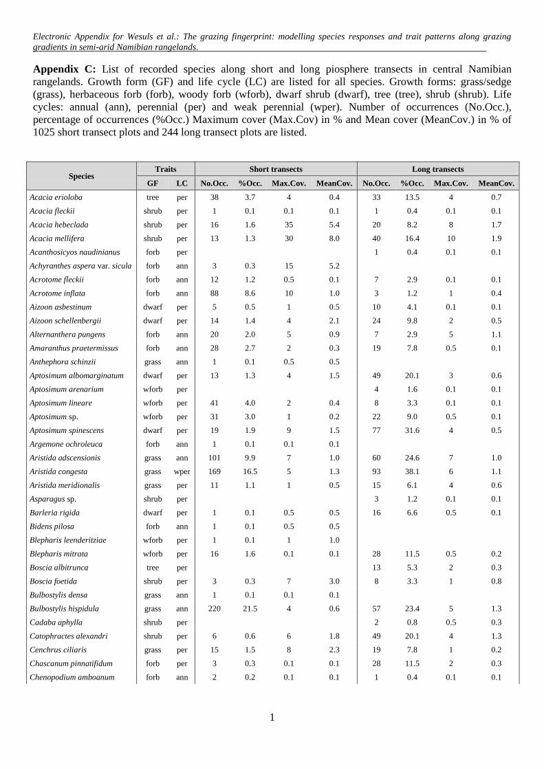
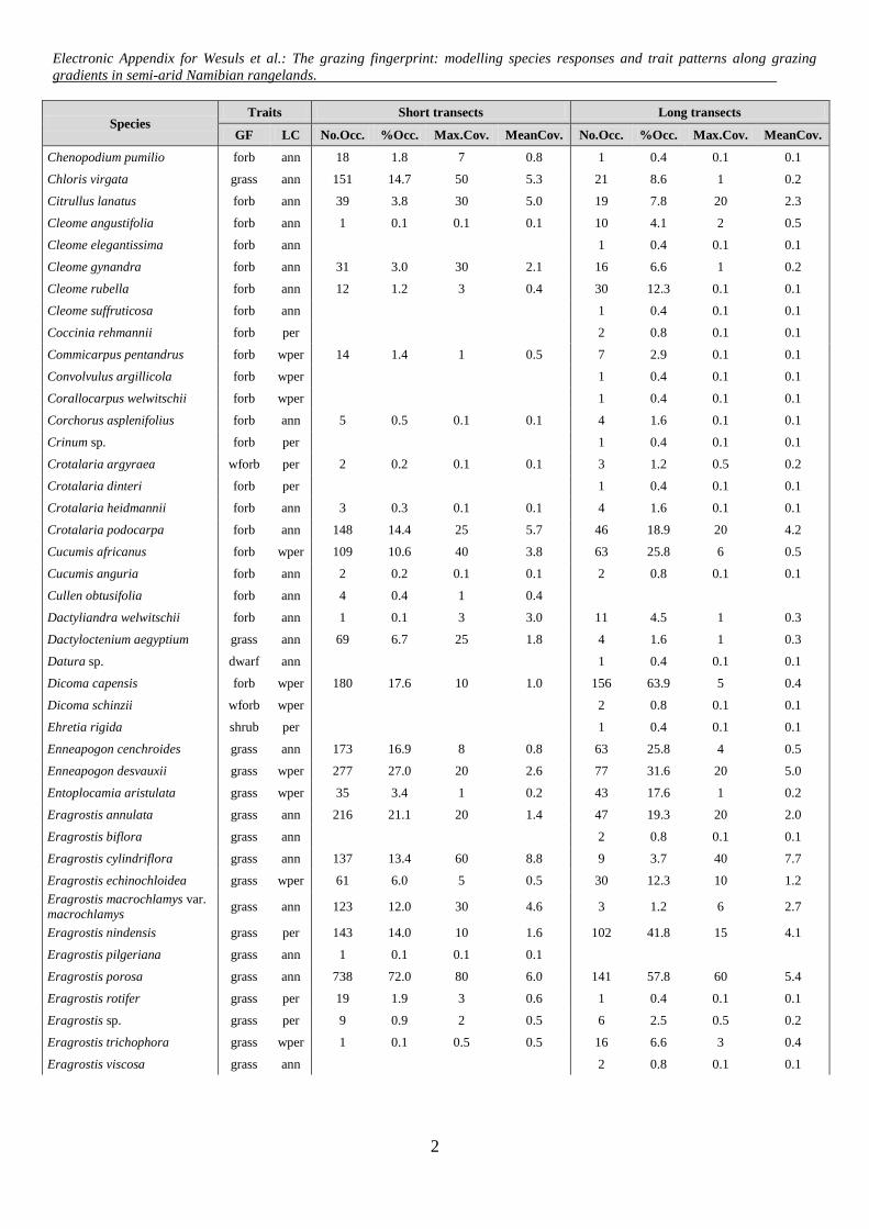
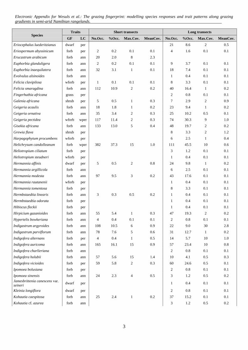
Appendix C: List of recorded species along short and long piosphere transects in central Namibian
rangelands. Growth form (GF) and life cycle (LC) are listed for all species. Growth forms: grass/sedge
(grass), herbaceous forb (forb), woody forb (wforb), dwarf shrub (dwarf), tree (tree), shrub (shrub). Life
cycles: annual (ann), perennial (per) and weak perennial (wper). Number of occurrences (No.Occ.),
percentage of occurrences (%Occ.) Maximum cover (Max.Cov) in % and Mean cover (MeanCov.) in % of
1025 short transect plots and 244 long transect plots are listed.
Species Traits Short transects Long transects
GF LC No.Occ. %Occ. Max.Cov. MeanCov. No.Occ. %Occ. Max.Cov. MeanCov.
Acacia erioloba tree per 38 3.7 4 0.4 33 13.5 4 0.7
Acacia fleckii shrub per 1 0.1 0.1 0.1 1 0.4 0.1 0.1
Acacia hebeclada shrub per 16 1.6 35 5.4 20 8.2 8 1.7
Acacia mellifera shrub per 13 1.3 30 8.0 40 16.4 10 1.9
Acanthosicyos naudinianus forb per 1 0.4 0.1 0.1
Achyranthes aspera var. sicula forb ann 3 0.3 15 5.2
Acrotome fleckii forb ann 12 1.2 0.5 0.1 7 2.9 0.1 0.1
Acrotome inflata forb ann 88 8.6 10 1.0 3 1.2 1 0.4
Aizoon asbestinum dwarf per 5 0.5 1 0.5 10 4.1 0.1 0.1
Aizoon schellenbergii dwarf per 14 1.4 4 2.1 24 9.8 2 0.5
Alternanthera pungens forb ann 20 2.0 5 0.9 7 2.9 5 1.1
Amaranthus praetermissus forb ann 28 2.7 2 0.3 19 7.8 0.5 0.1
Anthephora schinzii grass ann 1 0.1 0.5 0.5
Aptosimum albomarginatum dwarf per 13 1.3 4 1.5 49 20.1 3 0.6
Aptosimum arenarium wforb per 4 1.6 0.1 0.1
Aptosimum lineare wforb per 41 4.0 2 0.4 8 3.3 0.1 0.1
Aptosimum sp. wforb per 31 3.0 1 0.2 22 9.0 0.5 0.1
Aptosimum spinescens dwarf per 19 1.9 9 1.5 77 31.6 4 0.5
Argemone ochroleuca forb ann 1 0.1 0.1 0.1
Aristida adscensionis grass ann 101 9.9 7 1.0 60 24.6 7 1.0
Aristida congesta grass wper 169 16.5 5 1.3 93 38.1 6 1.1
Aristida meridionalis grass per 11 1.1 1 0.5 15 6.1 4 0.6
Asparagus sp. shrub per 3 1.2 0.1 0.1
Barleria rigida dwarf per 1 0.1 0.5 0.5 16 6.6 0.5 0.1
Bidens pilosa forb ann 1 0.1 0.5 0.5
Blepharis leenderitziae wforb per 1 0.1 1 1.0
Blepharis mitrata wforb per 16 1.6 0.1 0.1 28 11.5 0.5 0.2
Boscia albitrunca tree per 13 5.3 2 0.3
Boscia foetida shrub per 3 0.3 7 3.0 8 3.3 1 0.8
Bulbostylis densa grass ann 1 0.1 0.1 0.1
Bulbostylis hispidula grass ann 220 21.5 4 0.6 57 23.4 5 1.3
Cadaba aphylla shrub per 2 0.8 0.5 0.3
Catophractes alexandri shrub per 6 0.6 6 1.8 49 20.1 4 1.3
Cenchrus ciliaris grass per 15 1.5 8 2.3 19 7.8 1 0.2
Chascanum pinnatifidum forb per 3 0.3 0.1 0.1 28 11.5 2 0.3
Chenopodium amboanum forb ann 2 0.2 0.1 0.1 1 0.4 0.1 0.1
Electronic Appendix for Wesuls et al.: The grazing fingerprint: modelling species responses and trait patterns along grazing
gradients in semi-arid Namibian rangelands.
2
Species Traits Short transects Long transects
GF LC No.Occ. %Occ. Max.Cov. MeanCov. No.Occ. %Occ. Max.Cov. MeanCov.
Chenopodium pumilio forb ann 18 1.8 7 0.8 1 0.4 0.1 0.1
Chloris virgata grass ann 151 14.7 50 5.3 21 8.6 1 0.2
Citrullus lanatus forb ann 39 3.8 30 5.0 19 7.8 20 2.3
Cleome angustifolia forb ann 1 0.1 0.1 0.1 10 4.1 2 0.5
Cleome elegantissima forb ann 1 0.4 0.1 0.1
Cleome gynandra forb ann 31 3.0 30 2.1 16 6.6 1 0.2
Cleome rubella forb ann 12 1.2 3 0.4 30 12.3 0.1 0.1
Cleome suffruticosa forb ann 1 0.4 0.1 0.1
Coccinia rehmannii forb per 2 0.8 0.1 0.1
Commicarpus pentandrus forb wper 14 1.4 1 0.5 7 2.9 0.1 0.1
Convolvulus argillicola forb wper 1 0.4 0.1 0.1
Corallocarpus welwitschii forb wper 1 0.4 0.1 0.1
Corchorus asplenifolius forb ann 5 0.5 0.1 0.1 4 1.6 0.1 0.1
Crinum sp. forb per 1 0.4 0.1 0.1
Crotalaria argyraea wforb per 2 0.2 0.1 0.1 3 1.2 0.5 0.2
Crotalaria dinteri forb per 1 0.4 0.1 0.1
Crotalaria heidmannii forb ann 3 0.3 0.1 0.1 4 1.6 0.1 0.1
Crotalaria podocarpa forb ann 148 14.4 25 5.7 46 18.9 20 4.2
Cucumis africanus forb wper 109 10.6 40 3.8 63 25.8 6 0.5
Cucumis anguria forb ann 2 0.2 0.1 0.1 2 0.8 0.1 0.1
Cullen obtusifolia forb ann 4 0.4 1 0.4
Dactyliandra welwitschii forb ann 1 0.1 3 3.0 11 4.5 1 0.3
Dactyloctenium aegyptium grass ann 69 6.7 25 1.8 4 1.6 1 0.3
Datura sp. dwarf ann 1 0.4 0.1 0.1
Dicoma capensis forb wper 180 17.6 10 1.0 156 63.9 5 0.4
Dicoma schinzii wforb wper 2 0.8 0.1 0.1
Ehretia rigida shrub per 1 0.4 0.1 0.1
Enneapogon cenchroides grass ann 173 16.9 8 0.8 63 25.8 4 0.5
Enneapogon desvauxii grass wper 277 27.0 20 2.6 77 31.6 20 5.0
Entoplocamia aristulata grass wper 35 3.4 1 0.2 43 17.6 1 0.2
Eragrostis annulata grass ann 216 21.1 20 1.4 47 19.3 20 2.0
Eragrostis biflora grass ann 2 0.8 0.1 0.1
Eragrostis cylindriflora grass ann 137 13.4 60 8.8 9 3.7 40 7.7
Eragrostis echinochloidea grass wper 61 6.0 5 0.5 30 12.3 10 1.2
Eragrostis macrochlamys var.
macrochlamys grass ann 123 12.0 30 4.6 3 1.2 6 2.7
Eragrostis nindensis grass per 143 14.0 10 1.6 102 41.8 15 4.1
Eragrostis pilgeriana grass ann 1 0.1 0.1 0.1
Eragrostis porosa grass ann 738 72.0 80 6.0 141 57.8 60 5.4
Eragrostis rotifer grass per 19 1.9 3 0.6 1 0.4 0.1 0.1
Eragrostis sp. grass per 9 0.9 2 0.5 6 2.5 0.5 0.2
Eragrostis trichophora grass wper 1 0.1 0.5 0.5 16 6.6 3 0.4
Eragrostis viscosa grass ann 2 0.8 0.1 0.1
Electronic Appendix for Wesuls et al.: The grazing fingerprint: modelling species responses and trait patterns along grazing
gradients in semi-arid Namibian rangelands.
3
Species Traits Short transects Long transects
GF LC No.Occ. %Occ. Max.Cov. MeanCov. No.Occ. %Occ. Max.Cov. MeanCov.
Eriocephalus luederitzianus dwarf per 21 8.6 2 0.5
Eriospermum abyssinicum forb per 2 0.2 0.1 0.1 4 1.6 0.1 0.1
Erucastrum arabicum forb ann 20 2.0 8 2.3
Euphorbia glanduligera forb ann 2 0.2 0.1 0.1 9 3.7 0.1 0.1
Euphorbia inaequilatera forb ann 32 3.1 1 0.1 18 7.4 0.1 0.1
Evolvulus alsinoides forb ann 1 0.4 0.1 0.1
Felicia clavipilosa wforb per 1 0.1 0.1 0.1 8 3.3 0.1 0.1
Felicia smaragdina forb ann 112 10.9 2 0.2 40 16.4 1 0.2
Fingerhuthia africana grass per 2 0.8 0.1 0.1
Galenia africana shrub per 5 0.5 1 0.3 7 2.9 2 0.9
Geigeria acaulis forb ann 18 1.8 1 0.2 23 9.4 1 0.2
Geigeria ornativa forb ann 35 3.4 2 0.3 25 10.2 0.5 0.1
Geigeria pectidea wforb wper 117 11.4 2 0.3 74 30.3 9 1.0
Gisekia africana forb ann 133 13.0 5 0.4 48 19.7 2 0.2
Grewia flava shrub per 8 3.3 2 1.2
Harpagophytum procumbens wforb per 6 2.5 1 0.4
Helichrysum candolleanum forb wper 382 37.3 15 1.0 111 45.5 10 0.6
Heliotropium ciliatum forb per 3 1.2 0.1 0.1
Heliotropium steudneri wforb per 1 0.4 0.1 0.1
Hermannia affinis dwarf per 5 0.5 2 0.8 24 9.8 1 0.2
Hermannia argillicola forb ann 6 2.5 0.1 0.1
Hermannia modesta forb ann 97 9.5 3 0.2 43 17.6 0.1 0.1
Hermannia rautanenii wforb per 1 0.4 0.1 0.1
Hermannia tomentosa forb per 8 3.3 0.1 0.1
Hermbstaedtia linearis forb ann 3 0.3 0.5 0.2 1 0.4 0.1 0.1
Hermbstaedtia odorata forb per 1 0.4 0.1 0.1
Hibiscus fleckii forb per 1 0.4 0.1 0.1
Hirpicium gazanioides forb ann 55 5.4 1 0.3 47 19.3 2 0.2
Hypertelis bowkeriana forb ann 4 0.4 0.1 0.1 2 0.8 0.1 0.1
Indigastrum argyroides forb ann 108 10.5 6 0.9 22 9.0 30 2.8
Indigastrum parviflorum forb ann 78 7.6 5 0.6 31 12.7 1 0.2
Indigofera alternans forb per 4 0.4 1 0.5 14 5.7 10 1.0
Indigofera auricoma forb ann 165 16.1 15 0.9 57 23.4 10 0.8
Indigofera charlieriana forb ann 2 0.8 0.1 0.1
Indigofera holubii forb ann 57 5.6 15 1.4 10 4.1 0.5 0.3
Indigofera vicioides forb per 59 5.8 2 0.3 60 24.6 0.5 0.1
Ipomoea bolusiana forb per 2 0.8 0.1 0.1
Ipomoea sinensis forb ann 24 2.3 4 0.5 3 1.2 0.5 0.2
Jamesbrittenia canescens var.
seineri dwarf per 1 0.4 0.1 0.1
Kleinia longiflora dwarf per 2 0.8 0.1 0.1
Kohautia caespitosa forb ann 25 2.4 1 0.2 37 15.2 0.1 0.1
Kohautia cf. azurea forb ann 3 1.2 0.5 0.2
Electronic Appendix for Wesuls et al.: The grazing fingerprint: modelling species responses and trait patterns along grazing
gradients in semi-arid Namibian rangelands.
4
Species Traits Short transects Long transects
GF LC No.Occ. %Occ. Max.Cov. MeanCov. No.Occ. %Occ. Max.Cov. MeanCov.
Kyllinga alba grass per 12 1.2 2 0.9 48 19.7 0.5 0.2
Kyphocarpa angustifolia forb ann 1 0.4 0.1 0.1
Laggera decurrens wforb wper 5 0.5 5 1.2 15 6.1 0.5 0.2
Ledebouria sp. forb per 3 1.2 0.1 0.1
Leucas pechuelii forb ann 3 1.2 0.5 0.2
Leucosphaera bainesii dwarf per 10 1.0 20 4.5 36 14.8 11 2.3
Limeum aethiopicum wforb wper 2 0.2 0.5 0.3 9 3.7 0.1 0.1
Limeum argute-carinatum forb ann 322 31.4 15 1.6 62 25.4 4 0.4
Limeum fenestratum forb ann 15 1.5 0.5 0.2 6 2.5 0.1 0.1
Limeum myosotis forb ann 75 7.3 6 1.0 32 13.1 4 0.6
Limeum pterocarpum forb ann 9 0.9 0.5 0.2 9 3.7 0.1 0.1
Limeum sulcatum forb ann 2 0.8 0.1 0.1
Lophiocarpus tenuissimus wforb wper 1 0.4 0.1 0.1
Lotononis platycarpa forb ann 194 18.9 25 1.3 66 27.0 4 0.5
Lycium eenii shrub per 5 0.5 4 1.6 36 14.8 2 0.8
Lycium hirsutum shrub per 1 0.1 3 3.0
Lycium oxycarpum shrub per 7 0.7 25 8.3 25 10.2 8 1.7
Melhania virescens wforb wper 12 1.2 0.5 0.1 4 1.6 0.1 0.1
Melinis repens grass ann 13 1.3 5 0.8 15 6.1 0.1 0.1
Melolobium adenodes dwarf wper 6 2.5 0.1 0.1
Melolobium microphyllum dwarf wper 15 1.5 2 0.4 3 1.2 0.1 0.1
Microchloa caffra grass per 14 1.4 1 0.3 28 11.5 8 0.5
Mollugo cerviana forb ann 41 4.0 0.1 0.1 9 3.7 0.1 0.1
Monechma divaricatum wforb wper 3 0.3 0.5 0.2 7 2.9 0.1 0.1
Monechma genistifolium dwarf per 59 5.8 25 4.3 46 18.9 10 2.3
Monechma spartioides wforb wper 3 0.3 0.1 0.1 1 0.4 0.1 0.1
Monelytrum luederitzianum grass per 1 0.4 0.1 0.1
Monsonia angustifolia forb ann 1 0.4 1 1.0
Monsonia senegalensis forb ann 1 0.1 3 3.0 10 4.1 0.5 0.1
Monsonia umbellata forb ann 29 2.8 3 0.6 30 12.3 3 0.6
Nelsia quadrangula forb ann 9 0.9 2 0.4 10 4.1 0.1 0.1
Nidorella resedifolia forb ann 8 0.8 2 0.4 37 15.2 0.5 0.1
Nymania capensis shrub per 1 0.1 0.1 0.1 1 0.4 0.1 0.1
Ocimum americanum var.
americanum dwarf wper 7 0.7 0.5 0.3 25 10.2 3 0.5
Ondetia linearis forb ann 7 0.7 0.5 0.2 16 6.6 2 0.4
Oropetium capense grass per 6 0.6 0.1 0.1 8 3.3 0.5 0.2
Osteospermum muricatum
subsp. muricatum forb ann 7 0.7 3 0.5 1 0.4 0.1 0.1
Otoptera burchellii wforb per 2 0.8 0.1 0.1
Oxygonum alatum forb ann 1 0.1 0.1 0.1
Panicum arbusculum grass per 1 0.1 3 3.0 1 0.4 0.1 0.1
Panicum lanipes grass per 1 0.4 0.1 0.1
Parkinsonia africana shrub per 2 0.8 0.1 0.1
Electronic Appendix for Wesuls et al.: The grazing fingerprint: modelling species responses and trait patterns along grazing
gradients in semi-arid Namibian rangelands.
5
Species Traits Short transects Long transects
GF LC No.Occ. %Occ. Max.Cov. MeanCov. No.Occ. %Occ. Max.Cov. MeanCov.
Pavonia burchellii wforb wper 1 0.1 0.1 0.1 5 2.0 0.5 0.2
Pegolettia pinnatilobata wforb wper 2 0.2 0.5 0.3
Pegolettia senegalensis forb ann 41 4.0 1 0.2 2 0.8 0.1 0.1
Pelargonium leucophyllum forb wper 1 0.4 0.1 0.1
Peliostomum leucorrhizum wforb wper 5 0.5 0.1 0.1 14 5.7 0.1 0.1
Pentarrhinum insipidum forb per 2 0.8 0.1 0.1
Pentzia calva dwarf per 6 0.6 6 2.1 10 4.1 0.5 0.2
Pergularia daemia forb per 1 0.4 0.1 0.1
Phaeoptilum spinosum shrub per 41 4.0 40 8.1 122 50.0 10 2.4
Phyllanthus maderaspatensis wforb wper 1 0.1 0.1 0.1 1 0.4 0.1 0.1
Phyllanthus pentandrus wforb per 1 0.1 0.1 0.1
Platycarpha carlinoides forb per 12 1.2 3 0.8 20 8.2 0.5 0.1
Pogonarthria fleckii grass ann 113 11.0 10 0.7 30 12.3 1 0.3
Pollichia campestris dwarf per 6 2.5 0.5 0.2
Polygala leptophylla wforb wper 5 0.5 0.1 0.1 5 2.0 0.1 0.1
Pseudogaltonia clavata forb per 7 0.7 2 1.2 25 10.2 1 0.5
Pteronia mucronata dwarf per 1 0.1 4 4.0
Ptycholobium biflorum wforb wper 7 0.7 1 0.4 8 3.3 0.1 0.1
Pupalia lappacea forb ann 1 0.4 0.5 0.5
Requienia sphaerosperma forb per 3 1.2 0.5 0.2
Rhigozum trichotomum shrub per 69 6.7 30 5.2 100 41.0 10 2.7
Schkuhria pinnata forb ann 15 1.5 15 1.9
Schmidtia kalahariensis grass ann 627 61.2 40 5.0 170 69.7 40 5.4
Schmidtia pappophoroides grass per 8 3.3 1 0.2
Seddera suffruticosa forb per 2 0.8 0.1 0.1
Selago dinteri forb per 1 0.4 0.1 0.1
Senecio consanguineus forb ann 60 5.9 7 0.7 26 10.7 1 0.2
Senna italica wforb per 2 0.8 0.1 0.1
Sericorema sericea forb ann 18 1.8 2 0.6 12 4.9 0.5 0.1
Sesamum triphyllum forb ann 87 8.5 2 0.3 60 24.6 0.5 0.1
Setaria verticillata grass ann 70 6.8 55 4.4 16 6.6 5 0.9
Sida ovata wforb wper 6 0.6 0.5 0.2 13 5.3 0.5 0.2
Solanum capense dwarf per 4 0.4 4 2.1 5 2.0 1 0.4
Solanum delagoense wforb per 2 0.8 0.1 0.1
Sporobolus nervosus grass per 4 1.6 0.1 0.1
Stipagrostis anomala grass wper 1 0.4 0.1 0.1
Stipagrostis ciliata grass per 40 3.9 8 1.9 63 25.8 20 2.9
Stipagrostis hirtigluma grass wper 1 0.1 0.1 0.1 5 2.0 0.1 0.1
Stipagrostis hochstetteriana grass per 10 1.0 4 1.4 21 8.6 8 1.1
Stipagrostis obtusa grass per 154 15.0 60 4.9 57 23.4 30 12.6
Stipagrostis uniplumis grass per 308 30.0 50 2.8 199 81.6 50 10.1
Tagetes minuta forb ann 9 0.9 5 0.7 1 0.4 0.1 0.1
Talinum arnotii forb per 1 0.1 0.1 0.1 32 13.1 0.1 0.1
Electronic Appendix for Wesuls et al.: The grazing fingerprint: modelling species responses and trait patterns along grazing
gradients in semi-arid Namibian rangelands.
6
Species Traits Short transects Long transects
GF LC No.Occ. %Occ. Max.Cov. MeanCov. No.Occ. %Occ. Max.Cov. MeanCov.
Tapinanthus oleifolius dwarf per 6 2.5 0.1 0.1
Tephrosia burchellii forb ann 3 0.3 0.5 0.2 11 4.5 0.1 0.1
Tephrosia dregeana wforb wper 12 1.2 0.5 0.2 20 8.2 0.1 0.1
Tetragonia calycina wforb per 2 0.2 0.5 0.3 1 0.4 0.1 0.1
Tragus berteronianus grass ann 161 15.7 5 0.6 51 20.9 10 0.6
Trianthema parvifolia forb ann 5 0.5 0.5 0.2 8 3.3 0.1 0.1
Tribulus cristatus forb wper 44 4.3 20 2.9 10 4.1 7 1.1
Tribulus pterophorus forb wper 9 3.7 0.1 0.1
Tribulus terrestris forb ann 201 19.6 90 10.2 56 23.0 60 5.3
Tribulus zeyheri forb wper 4 0.4 0.1 0.1 3 1.2 0.1 0.1
Trichogyne cf. paronychioides forb ann 3 0.3 0.1 0.1 5 2.0 0.1 0.1
Triraphis purpurea grass ann 12 1.2 1 0.4
Urochloa brachyura grass ann 17 1.7 20 2.4 1 0.4 0.1 0.1
Urochloa panicoides grass ann 1 0.1 0.5 0.5 1 0.4 0.1 0.1
Ursinia nana forb ann 7 0.7 1 0.2 4 1.6 0.1 0.1
Xerophyta humilis forb per 1 0.1 3 3.0 4 1.6 0.1 0.1
Zehneria marlothii forb ann 1 0.4 0.1 0.1
Ziziphus mucronata tree per 1 0.4 0.1 0.1
Zygophyllum suffruticosum dwarf per 3 1.2 0.5 0.4
Zygophyllum tenue dwarf per 1 0.1 2 2.0
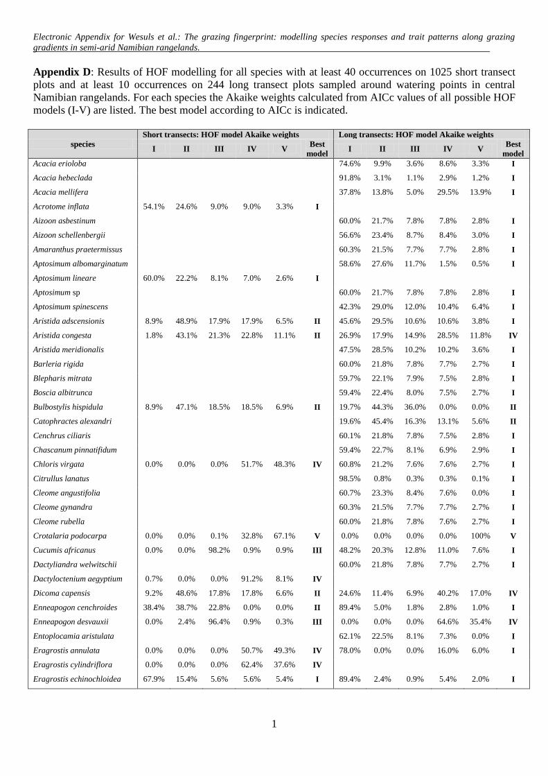
Electronic Appendix for Wesuls et al.: The grazing fingerprint: modelling species responses and trait patterns along grazing
gradients in semi-arid Namibian rangelands.
1
Appendix D: Results of HOF modelling for all species with at least 40 occurrences on 1025 short transect
plots and at least 10 occurrences on 244 long transect plots sampled around watering points in central
Namibian rangelands. For each species the Akaike weights calculated from AICc values of all possible HOF
models (I-V) are listed. The best model according to AICc is indicated.
species
Short transects: HOF model Akaike weights Long transects: HOF model Akaike weights
I II III IV V Best
model I II III IV V
Best
model
Acacia erioloba 74.6% 9.9% 3.6% 8.6% 3.3% I
Acacia hebeclada 91.8% 3.1% 1.1% 2.9% 1.2% I
Acacia mellifera 37.8% 13.8% 5.0% 29.5% 13.9% I
Acrotome inflata 54.1% 24.6% 9.0% 9.0% 3.3% I
Aizoon asbestinum 60.0% 21.7% 7.8% 7.8% 2.8% I
Aizoon schellenbergii 56.6% 23.4% 8.7% 8.4% 3.0% I
Amaranthus praetermissus 60.3% 21.5% 7.7% 7.7% 2.8% I
Aptosimum albomarginatum 58.6% 27.6% 11.7% 1.5% 0.5% I
Aptosimum lineare 60.0% 22.2% 8.1% 7.0% 2.6% I
Aptosimum sp 60.0% 21.7% 7.8% 7.8% 2.8% I
Aptosimum spinescens 42.3% 29.0% 12.0% 10.4% 6.4% I
Aristida adscensionis 8.9% 48.9% 17.9% 17.9% 6.5% II 45.6% 29.5% 10.6% 10.6% 3.8% I
Aristida congesta 1.8% 43.1% 21.3% 22.8% 11.1% II 26.9% 17.9% 14.9% 28.5% 11.8% IV
Aristida meridionalis 47.5% 28.5% 10.2% 10.2% 3.6% I
Barleria rigida 60.0% 21.8% 7.8% 7.7% 2.7% I
Blepharis mitrata 59.7% 22.1% 7.9% 7.5% 2.8% I
Boscia albitrunca 59.4% 22.4% 8.0% 7.5% 2.7% I
Bulbostylis hispidula 8.9% 47.1% 18.5% 18.5% 6.9% II 19.7% 44.3% 36.0% 0.0% 0.0% II
Catophractes alexandri 19.6% 45.4% 16.3% 13.1% 5.6% II
Cenchrus ciliaris 60.1% 21.8% 7.8% 7.5% 2.8% I
Chascanum pinnatifidum 59.4% 22.7% 8.1% 6.9% 2.9% I
Chloris virgata 0.0% 0.0% 0.0% 51.7% 48.3% IV 60.8% 21.2% 7.6% 7.6% 2.7% I
Citrullus lanatus 98.5% 0.8% 0.3% 0.3% 0.1% I
Cleome angustifolia 60.7% 23.3% 8.4% 7.6% 0.0% I
Cleome gynandra 60.3% 21.5% 7.7% 7.7% 2.7% I
Cleome rubella 60.0% 21.8% 7.8% 7.6% 2.7% I
Crotalaria podocarpa 0.0% 0.0% 0.1% 32.8% 67.1% V 0.0% 0.0% 0.0% 0.0% 100% V
Cucumis africanus 0.0% 0.0% 98.2% 0.9% 0.9% III 48.2% 20.3% 12.8% 11.0% 7.6% I
Dactyliandra welwitschii 60.0% 21.8% 7.8% 7.7% 2.7% I
Dactyloctenium aegyptium 0.7% 0.0% 0.0% 91.2% 8.1% IV
Dicoma capensis 9.2% 48.6% 17.8% 17.8% 6.6% II 24.6% 11.4% 6.9% 40.2% 17.0% IV
Enneapogon cenchroides 38.4% 38.7% 22.8% 0.0% 0.0% II 89.4% 5.0% 1.8% 2.8% 1.0% I
Enneapogon desvauxii 0.0% 2.4% 96.4% 0.9% 0.3% III 0.0% 0.0% 0.0% 64.6% 35.4% IV
Entoplocamia aristulata 62.1% 22.5% 8.1% 7.3% 0.0% I
Eragrostis annulata 0.0% 0.0% 0.0% 50.7% 49.3% IV 78.0% 0.0% 0.0% 16.0% 6.0% I
Eragrostis cylindriflora 0.0% 0.0% 0.0% 62.4% 37.6% IV
Eragrostis echinochloidea 67.9% 15.4% 5.6% 5.6% 5.4% I 89.4% 2.4% 0.9% 5.4% 2.0% I
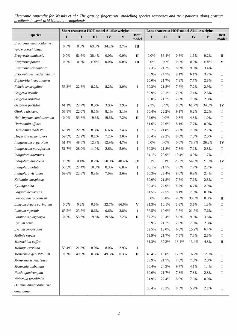
Electronic Appendix for Wesuls et al.: The grazing fingerprint: modelling species responses and trait patterns along grazing
gradients in semi-arid Namibian rangelands.
2
species
Short transects: HOF model Akaike weights Long transects: HOF model Akaike weights
I II III IV V Best
model I II III IV V
Best
model
Eragrostis macrochlamys
var. macrochlamys 0.0% 0.0% 63.0% 34.2% 2.7% III
Eragrostis nindensis 0.0% 61.6% 38.4% 0.0% 0.0% II 0.0% 88.4% 0.8% 1.6% 9.2% II
Eragrostis porosa 0.0% 0.0% 100% 0.0% 0.0% III 0.0% 0.0% 0.0% 0.0% 100% V
Eragrostis trichophora 57.3% 21.2% 8.6% 9.5% 3.4% I
Eriocephalus luederitzianus 56.9% 24.7% 9.1% 6.1% 3.2% I
Euphorbia inaequilatera 60.0% 21.7% 7.8% 7.7% 2.8% I
Felicia smaragdina 58.3% 22.3% 8.2% 8.2% 3.0% I 60.3% 21.8% 7.8% 7.2% 2.9% I
Geigeria acaulis 59.9% 22.1% 7.9% 7.4% 2.6% I
Geigeria ornativa 60.0% 21.7% 7.8% 7.8% 2.8% I
Geigeria pectidea 61.1% 22.7% 8.3% 3.9% 3.9% I 2.3% 0.9% 0.3% 61.7% 34.8% IV
Gisekia africana 58.8% 22.0% 8.1% 8.1% 3.1% I 60.4% 22.2% 9.1% 6.2% 2.2% I
Helichrysum candolleanum 0.0% 53.6% 19.6% 19.6% 7.2% II 94.0% 0.0% 0.3% 4.8% 1.0% I
Hermannia affinis 61.6% 22.6% 8.1% 7.7% 0.0% I
Hermannia modesta 60.1% 22.6% 8.3% 6.6% 2.4% I 60.2% 21.8% 7.8% 7.5% 2.7% I
Hirpicium gazanioides 59.5% 22.2% 8.1% 7.2% 3.0% I 60.4% 22.2% 8.0% 7.0% 2.5% I
Indigastrum argyroides 51.4% 48.6% 12.8% 12.9% 4.7% I 0.0% 0.0% 0.0% 73.8% 26.2% IV
Indigastrum parviflorum 51.7% 28.9% 11.9% 2.6% 5.0% I 60.3% 21.8% 7.8% 7.2% 2.8% I
Indigofera alternans 54.1% 28.9% 10.4% 4.9% 1.7% I
Indigofera auricoma 1.0% 0.4% 0.2% 50.0% 48.4% IV 0.1% 0.1% 23.2% 54.8% 21.8% IV
Indigofera holubii 55.5% 27.4% 10.0% 0.3% 6.8% I 60.1% 21.7% 7.8% 7.7% 2.7% I
Indigofera vicioides 59.6% 22.6% 8.3% 7.0% 2.6% I 60.3% 22.4% 8.0% 6.9% 2.4% I
Kohautia caespitosa 60.0% 21.8% 7.8% 7.6% 2.8% I
Kyllinga alba 59.3% 22.9% 8.2% 6.7% 2.9% I
Laggera decurrens 61.5% 22.5% 8.1% 7.9% 0.0% I
Leucosphaera bainesii 0.0% 56.8% 9.6% 33.6% 0.0% II
Limeum argute carinatum 0.0% 0.2% 0.5% 32.7% 66.6% V 81.3% 10.1% 3.6% 3.6% 1.3% I
Limeum myosotis 63.5% 23.5% 8.6% 0.6% 3.8% I 56.5% 10.6% 3.8% 21.5% 7.6% I
Lotononis platycarpa 0.0% 53.6% 19.6% 19.6% 7.2% II 57.2% 22.4% 8.0% 9.0% 3.3% I
Lycium eenii 59.9% 21.7% 7.8% 7.8% 2.8% I
Lycium oxycarpum 52.5% 19.0% 6.8% 15.2% 6.4% I
Melinis repens 59.9% 21.7% 7.8% 7.8% 2.8% I
Microchloa caffra 31.3% 37.2% 13.4% 13.4% 4.8% II
Mollugo cerviana 59.4% 21.8% 8.0% 8.0% 2.9% I
Monechma genistifolium 0.3% 49.5% 0.3% 49.5% 0.3% II 40.4% 13.0% 17.2% 16.7% 12.8% I
Monsonia senegalensis 59.9% 21.7% 7.8% 7.8% 2.8% I
Monsonia umbellata 60.4% 24.3% 9.7% 4.1% 1.4% I
Nelsia quadrangula 60.0% 21.7% 7.8% 7.8% 2.8% I
Nidorella resedifolia 61.9% 22.4% 8.0% 7.6% 0.0% I
Ocimum americanum var.
americanum 60.4% 23.3% 8.3% 5.9% 2.1% I
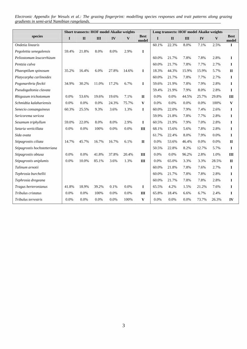
Electronic Appendix for Wesuls et al.: The grazing fingerprint: modelling species responses and trait patterns along grazing
gradients in semi-arid Namibian rangelands.
3
species
Short transects: HOF model Akaike weights Long transects: HOF model Akaike weights
I II III IV V Best
model I II III IV V
Best
model
Ondetia linearis 60.1% 22.3% 8.0% 7.1% 2.5% I
Pegolettia senegalensis 59.4% 21.8% 8.0% 8.0% 2.9% I
Peliostomum leucorrhizum 60.0% 21.7% 7.8% 7.8% 2.8% I
Pentzia calva 60.0% 21.7% 7.8% 7.7% 2.7% I
Phaeoptilum spinosum 35.2% 16.4% 6.0% 27.8% 14.6% I 18.3% 44.3% 15.9% 15.9% 5.7% II
Platycarpha carlinoides 60.0% 21.7% 7.8% 7.7% 2.7% I
Pogonarthria fleckii 34.9% 30.2% 11.0% 17.2% 6.7% I 59.6% 21.9% 7.8% 7.9% 2.8% I
Pseudogaltonia clavata 59.4% 21.9% 7.9% 8.0% 2.8% I
Rhigozum trichotomum 0.0% 53.6% 19.6% 19.6% 7.1% II 0.0% 0.0% 44.5% 25.7% 29.8% III
Schmidtia kalahariensis 0.0% 0.0% 0.0% 24.3% 75.7% V 0.0% 0.0% 0.0% 0.0% 100% V
Senecio consanguineus 60.3% 25.5% 9.3% 3.6% 1.3% I 60.0% 22.0% 7.9% 7.4% 2.6% I
Sericorema sericea 59.9% 21.8% 7.8% 7.7% 2.8% I
Sesamum triphyllum 59.0% 22.0% 8.0% 8.0% 2.9% I 60.5% 21.9% 7.9% 7.0% 2.8% I
Setaria verticillata 0.0% 0.0% 100% 0.0% 0.0% III 68.1% 15.6% 5.6% 7.8% 2.8% I
Sida ovata 61.7% 22.4% 8.0% 7.9% 0.0% I
Stipagrostis ciliata 14.7% 45.7% 16.7% 16.7% 6.1% II 0.0% 53.6% 46.4% 0.0% 0.0% II
Stipagrostis hochstetteriana 50.5% 22.8% 8.2% 12.7% 5.7% I
Stipagrostis obtusa 0.0% 0.0% 41.8% 37.8% 20.4% III 0.0% 0.0% 96.2% 2.8% 1.0% III
Stipagrostis uniplumis 0.0% 10.0% 85.1% 3.6% 1.3% III 0.0% 65.0% 3.3% 3.3% 28.5% II
Talinum arnotii 60.0% 21.8% 7.8% 7.6% 2.7% I
Tephrosia burchellii 60.0% 21.7% 7.8% 7.8% 2.8% I
Tephrosia dregeana 60.0% 21.7% 7.8% 7.8% 2.8% I
Tragus berteronianus 41.8% 18.9% 39.2% 0.1% 0.0% I 65.5% 4.2% 1.5% 21.2% 7.6% I
Tribulus cristatus 0.0% 0.0% 100% 0.0% 0.0% III 65.8% 18.4% 6.6% 6.7% 2.4% I
Tribulus terrestris 0.0% 0.0% 0.0% 0.0% 100% V 0.0% 0.0% 0.0% 73.7% 26.3% IV
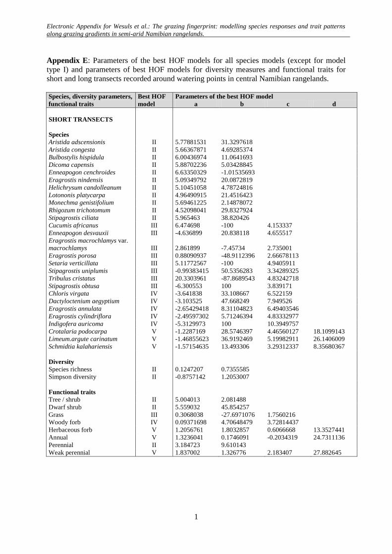
Electronic Appendix for Wesuls et al.: The grazing fingerprint: modelling species responses and trait patterns
along grazing gradients in semi-arid Namibian rangelands.
1
Appendix E: Parameters of the best HOF models for all species models (except for model
type I) and parameters of best HOF models for diversity measures and functional traits for
short and long transects recorded around watering points in central Namibian rangelands.
Species, diversity parameters, Best HOF Parameters of the best HOF model
functional traits model a b c d
SHORT TRANSECTS
Species
Aristida adscensionis II 5.77881531 31.3297618
Aristida congesta II 5.66367871 4.69285374
Bulbostylis hispidula II 6.00436974 11.0641693
Dicoma capensis II 5.88702236 5.03428845
Enneapogon cenchroides II 6.63350329 -1.01535693
Eragrostis nindensis II 5.09349792 20.0872819
Helichrysum candolleanum II 5.10451058 4.78724816
Lotononis platycarpa II 4.96490915 21.4516423
Monechma genistifolium II 5.69461225 2.14878072
Rhigozum trichotomum II 4.52098041 29.8327924
Stipagrostis ciliata II 5.965463 38.820426
Cucumis africanus III 6.474698 -100 4.153337
Enneapogon desvauxii III -4.636899 20.838118 4.655517
Eragrostis macrochlamys var.
macrochlamys III 2.861899 -7.45734 2.735001
Eragrostis porosa III 0.88090937 -48.9112396 2.66678113
Setaria verticillata III 5.11772567 -100 4.9405911
Stipagrostis uniplumis III -0.99383415 50.5356283 3.34289325
Tribulus cristatus III 20.3303961 -87.8689543 4.83242718
Stipagrostis obtusa III -6.300553 100 3.839171
Chloris virgata IV -3.641838 33.108667 6.522159
Dactyloctenium aegyptium IV -3.103525 47.668249 7.949526
Eragrostis annulata IV -2.65429418 8.31104823 6.49403546
Eragrostis cylindriflora IV -2.49597302 5.71246394 4.83332977
Indigofera auricoma IV -5.3129973 100 10.3949757
Crotalaria podocarpa V -1.2287169 28.5746397 4.46560127 18.1099143
Limeum.argute carinatum V -1.46855623 36.9192469 5.19982911 26.1406009
Schmidtia kalahariensis V -1.57154635 13.493306 3.29312337 8.35680367
Diversity
Species richness II 0.1247207 0.7355585
Simpson diversity II -0.8757142 1.2053007
Functional traits
Tree / shrub II 5.004013 2.081488
Dwarf shrub II 5.559032 45.854257
Grass III 0.3068038 -27.6971076 1.7560216
Woody forb IV 0.09371698 4.70648479 3.72814437
Herbaceous forb V 1.2056761 1.8032857 0.6066668 13.3527441
Annual V 1.3236041 0.1746091 -0.2034319 24.7311136
Perennial II 3.184723 9.610143
Weak perennial V 1.837002 1.326776 2.183407 27.882645
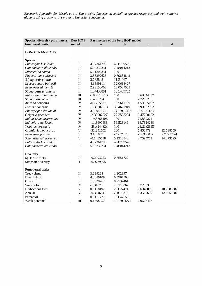
Electronic Appendix for Wesuls et al.: The grazing fingerprint: modelling species responses and trait patterns
along grazing gradients in semi-arid Namibian rangelands.
2
Species, diversity parameters, Best HOF Parameters of the best HOF model
functional traits model a b c d
LONG TRANSECTS
Species
Bulbostylis hispidula II 4.97364798 4.28769526
Catophractes alexandri II 5.00232231 7.48014213
Microchloa caffra II 5.21808351 100
Phaeoptilum spinosum II 3.83392625 0.79884843
Stipagrostis ciliata II 3.793848 11.51067
Leucosphaera bainesii II 4.18991114 32.0614427
Eragrostis nindensis II 2.92150003 13.0527565
Stipagrostis uniplumis II 1.04430881 18.5469702
Rhigozum trichotomum III -10.7513716 100 3.69744597
Stipagrostis obtusa III -14.30264 100 2.72352
Aristida congesta IV -0.1265087 19.5641739 4.53855192
Dicoma capensis IV -1.35702518 39.4621949 5.90162892
Enneapogon desvauxii IV 3.33946174 -3.92925403 -0.61904082
Geigeria pectidea IV -2.39087627 27.2508284 6.47208182
Indigastrum .argyroides IV -19.8766406 100 21.830274
Indigofera auricoma IV -11.3600983 59.523146 14.7324238
Tribulus terrestris IV -25.3244823 100 25.2062618
Crotalaria podocarpa V -32.351602 100 5.452479 12.528559
Eragrostis porosa V 3.181037 -2.232431 -59.353057 -67.587124
Schmidtia kalahariensis V -0.1485588 5.1210848 2.7595771 14.3731254
Bulbostylis hispidula II 4.97364798 4.28769526
Catophractes alexandri II 5.00232231 7.48014213
Diversity
Species richness II -0.2993253 0.7551722
Simpson diversity I -0.9779995
Functional traits
Tree / shrub II 3.239268 1.102897
Dwarf shrub II 4.3386109 0.5967508
Grass II 1.0528267 0.7732461
Woody forb IV -1.018796 20.119067 5.72553
Herbaceous forb V 0.6158192 2.5627471 3.6347099 18.7583087
Annual V -0.3546541 2.1678316 2.3519609 12.9851882
Perennial II 0.9117727 10.647555
Weak perennial III 0.1598957 -13.8921272 2.9626467