Embed Size (px)
Citation preview

The h-p Version of the Finite Element Method in
Three Dimensions
by
Jianming Zhang
A ThesisSubmitted to the Faculty of Graduate Studies
at the University of Manitoba
In Partial Fulfillment of the Requirements forthe Degree
Doctor of Philosophy
Department of Mathematics
University of Manitoba
Copyright c© 2008
i

Acknowledgements
I deeply thank my supervisor Dr. Benqi Guo for invaluable guidance, encouragement,patience and constant support throughout this program.
I would also like to thank the other members of my Advisor Committee: Dr. S. H. Lui,Dr. Ruppa Thulasiram and Dr. Bin Han. They have taken the time to read carefully thisthesis and provided many valuable suggestions.
I also thank the Department of Mathematics and Dr. Benqi Guo for their financialsupport during my graduate studies.
Finally, I would like to acknowledge all my family, especially my wife(Chen Deying), mydaughter(Zhang Xinyuan) and my parents for their continuing love and support.
ii

Contents
Acknowledgements ii
Abstract iv
Chapter 1. Introduction 1
Chapter 2. Preliminary 52.1. Jacobi Polynomial 52.2. Jacobi-weighted Sobolev and Besov spaces on Q = (−1, 1)3 72.3. Approximation Properties of Jacobi Projections 11
Chapter 3. Approximation Theory in Jacobi-weighted Spaces on a Scaled CubeQh = (−h, h)3 14
3.1. Jacobi-weighted Sobolev and Besov spaces on Qh = (−h, h)3 143.2. Approximation in the framework of Jacobi-weighted spaces on Qh = (−h, h)3 153.3. Approximability of singular functions on scaled cube Qh = (−h, h)3 18
Chapter 4. Polynomial Extensions in Three Dimensions 344.1. Extension on a standard triangular prisms 344.2. Extension on a standard pyramid 464.3. Extension on a standard cube 62
Chapter 5. The convergence of the h-p version of the Finite Element Method 775.1. A model boundary value problem 775.2. Adjustment of local projection polynomials at the vertices and edges 815.3. The convergence for elliptic problems with smooth solution in Hk(Ω) 895.4. The convergence for problems on polyhedral domains 102
Chapter 6. Computation and Applications of the h-p version of Finite ElementSolutions 114
6.1. Poission equation on polyhedral domains 1146.2. Three dimensional elasticity problems on polyhedral domains 137
Chapter 7. Conclusion 148
Bibliography 149
iii

Abstract
In the framework of the Jacobi-weighted Besov and Sobolev spaces, we analyze the ap-proximation to singular and smooth functions. We construct stable and compatible polyno-mial extensions from triangular and square faces to prisms, hexahedrons and pyramids, andintroduce quasi Jacobi projection operators on individual elements, which is a combinationof the Jacobi projection and the interpolation at vertices and on sides of elements. Applyingthese results we establish the convergence of the h-p version of the finite element methodwith quasi uniform meshes in three dimensions for elliptic problems with smooth solutionsor singular solutions on polyhedral domains in three dimensions. The rate of convergence interms of h and p is proved to be the best.
iv

CHAPTER 1
Introduction
The finite element method (FEM) has rapidly developed as an important numericalmethod for partial differential equations in theory, algorithm, and applications since the1940’s, and becomes now the mostly used computational tool to solve large-scale engineeringand scientific problems. In the early years, FEM was used in structural mechanics suchas civil engineering, automobile industry and aerospace industry, and it has penetratedalmost every field of today’s engineering and sciences, such as material science, electric-magnetic fields, fluid dynamics, biology, and finance. Numerous softwares of FEM have beensuccessfully used in industry, research and education such as MSC/NASTRAN, ANSYS,ABAQUS, COSMIC, and many others.
According to the structure of finite element solutions, there are three approaches of thefinite element method: the h-version, the p-version and the h-p version. In the h-version,the degree p of the elements is fixed at a low level and the accuracy is achieved by properlyrefining the mesh. In the p-version, the mesh is fixed and the degree p of polynomials is in-creased uniformly or selectively to achieve the accuracy. The h-p version is the combinationof the h-version and p-version, namely, refine meshes and increase polynomial degrees simul-taneously and selectively (or uniformly) in order to achieve higher accuracy. The p-versionand h-p version are new developments, commercial and research codes based on the p andh-p versions of FEM are now widely used in computational engineering and sciences, for ex-ample, the commercial codes Pro/MECHANICA, PolyFEM, ProPHLEX, STRESSCHECKand the research codes STRIPE, HP-2D and HP-3D.
The first theoretical paper on the p -version in two dimensions by Babuska, Szabo andKatz was published in the early 1980s, it was shown in [9] that the p-version of FEM convergesat least as fast as the classical FEM with quasi-uniform meshes and it converges twice as fastas the classical FEM if the solution has singularity of rγ-type. Babuska and Suri improved in[7] substantially the results of [9] and generalized to the h-p version in two dimensions in [8].A detailed analysis of the p and h-p version in one dimension was given by Gui and Babuska in[23]. Since then remarkable progresses for the p and h-p version in one and two dimensionswere made in the 1980s and 1990s, see e.g. [7, 8, 2, 19, 29, 30, 31, 41, 42, 44, 45],and the p and h-p version were implemented in commercial codes and used in practicalengineering computation. Despite these progresses, people had struggled for an appropriatemathematical framework which is able to provide a uniform error analysis for the p and h-pversion of FEM in one, two and three dimensions and to lead to the optimal convergenceof the FEM solutions of the p and h-p version for problems on polygonal and polyhedral
1

1. INTRODUCTION 2
domains. After two-decades effort people realize very recently that the most appropriatemathematical framework for error analysis of the p and h-p version is the Jacobi-weightedBesov and Sobolev spaces. In a series of papers by Guo and his collaborators [3, 4, 5, 6, 34],a new analysis of the p and h-p version was given in which the approximation theory of theFEM and BEM in two dimensions in this new mathematical framework was systematicallydeveloped. It demonstrates that Jacobi-weighted Besov space is the most appropriate tool toobtain optimal upper and lower bounds when dealing with singular solutions on polygons.This framework has been generalized to the p-version and the h-p version of the BEM[32, 33]. Thus the approximation theory for the p and h-p version of FEM and BEM in twodimensions has been established in the framework of the Jocobi-weighted Besov and Sobolevspaces.
Although significant progresses for the p and h-p versions FEM in one and two dimen-sions have been made in the past three decades, the approximation theory of the p and h-pversions of FEM in three dimensions is much less developed due to the complexity of threedimensional problems, and only a few results are available, e.g. [10, 16, 40]. There are threefundamental issues or difficulties in the analysis of high-order FEM in three dimensions. Firstof all, design three types of Jacobi-weighted Besov and Sobolev spaces such that the threetypes of singularities in three dimensions can be characterized precisely and the Jacobi pro-jections of the singular functions in these spaces lead to the sharpest approximation errors.Secondly, define local projection based operator which is a combination of Jacobi projectionand interpolation at vertices and sides of elements remaining the best approximation prop-erties of the Jacobi projection. At the third, establishing stable and compatible polynomialextensions of polynomials from faces of three commonly used elements in three dimensionswhich realize global continuity of piecewise polynomial and remain the best approximationof local Jacobi projections.
In despite of theoretical difficulties the computation and algorithms of the p and h-pFEM have made remarkable progresses in the past decades. As the computer power growsrapidly in speed and memory, many practical problems in engineering and sciences are mod-eled and computed in three dimensions, which were not feasible ten or twenty years ago.Because of the limitation on the capacity of computers many three dimensional problems inthe real world were reduced or simplified to two dimensional models for the computation,which substantially minimized the reliability of the prediction based on the computation forimportant engineering, scientific, public health, and financial decision. The high accuracy ofcomputational solutions on original three dimensional model problems significantly increasethe knowledge of problems in the real world, and make it possible to validate mathematicalmodels and to verify the computational results. Since the p and h-p versions FEM in threedimensions provide higher accuracy and reduce significantly computational cost, they havebeen applied to various fields of engineering and sciences such as mechanics, magnetoelec-tric, biology and material science [15, 37, 39, 43, 46], and have been implemented in newcodes and enhanced in the existing codes. These codes with three dimensional p and h-pFEM capacity have become very powerful tools to solve large scale engineering and scien-tific problems and play an important role in computational engineering and sciences. The

1. INTRODUCTION 3
success of the p and h-p FEM in computation is a great challenge to mathematicians andengineers, i.e., whether the theoretical research of the the p and h-p FEM in three dimensionscan provide a solid mathematical foundation and guidance for practical computations, e.g.verification of three dimensional FEM codes (commercial and research) and verification ofthe numerical results. This challenge has motivated researchers in recent years to establishnew mathematical framework for developing new approximation theory of high order FEMin three dimensions, and also provides significant motivation of the thesis, which is a partof the effort to establish a comprehensive understanding of the fundamental issues we arefacing now.
In this thesis, we shall develop the approximation theory of the h-p version of FEM withquasi-uniform meshes in three dimensions in the framework of the Jacobi-weighted Besovand Sobolev spaces. The h-p version with quasiuniform meshes is, from methodology andapproximation theory, the p-version on scaled meshes. The approach of the p-version givesthe p-dependence in the approximation errors, and a proper scaling argument will revealfully the information of the h-dependence. Hence, the analysis for the best approximationof the h-p version with quasiuniform meshes is not feasible unless the optimal convergenceof the p-version in three dimensions is established. Fortunately, a comprehensive analysisof the p-version in the framework of the Jacobi-weighted Besov and Sobolev spaces in threedimensions recently appears in a series of papers [24, 25] by Guo, we are now ready to pursuethe best error estimation for the h-p version in three dimensions. Here we incorporate themesh dependence into the analysis for the p-version, and provide optimal estimates for quasi-uniform meshes and quasi-uniform polynomial degrees.
We generalize the Jacobi-weighted Besov and Sobolev spaces on scaled cube Qh =(−h, h)3, and analyze the properties of Jacobi projection on Qh. The errors in Jacobi pro-jections with three different Jacobi weights for singular functions with vertex, edge andvertex-edge singularities are investigated in terms of h and p (polynomial degree), which arerigorously proved to be the sharpest.
Next we construct explicitly polynomial extensions on standard elements: cubes, trian-gular prisms and pyramids which are proved rigorously to be stable and compatible withFEM subspaces on tetrahedrons, cubes, triangular prisms and pyramids. The extensionsfrom a triangular face to a prism and from a square face to a pyramid are of convolution
type which realize continuous mappings: H1/200 (T )( or H
1/200 (S)) → H1(Ωst) where Ωst de-
notes one of these standard elements and T and S are triangular and square faces. Theextension on a cube is constructed by using spectral solutions of the eigenvalue problem ofPoisson equation on a square face S and two-point value problem on an interval I. Theextension from a square face to prism is quite different from those in other cases, the normof the extension depends on p , but it is compatible with local quasi-projection operator onprismatic elements and cause no loss of the rate of convergence of the finite element solutionof the p and h-p version.
The local quasi projection is based the Jacobi projection and associates with linearor trilinear interpolation at vertices of elements and with the H1/2 projection on each

1. INTRODUCTION 4
side of elements. These projections remain the sharp estimation of Jacobi projection andmake the difference of quasi projection on a common face of a pair of elements belong to
H1/200 (T )( or H
1/200 (S)), which make it possible to apply the polynomial extensions for conti-
nuity across the interfaces of elements.By utilizing the polynomial extensions and local quasi projections on tetrahedrons, cubes,
triangular prisms we proved the best convergence of the h-p FEM for problems with smoothsolutions. For the singular solutions for problems on polyhedral domains, we use Jacobi-weighted Besov and Sobolev spaces to characterize the various singularities and derivestheir best approximabilities. Combining the approximation results for smooth functions andsingular functions, we obtain the convergence rate of the h-p version of the finite elementmethod with quasi-uniform meshes for elliptic problems on polyhedral domains, where thesingularities of three different types occur and substantially govern the convergence of thefinite element solutions.
The rest of this thesis is organized as follows: In Chapter 2, we first review the proper-ties of Jacobi polynomial, then we quote important properties of Jacobi projections in threedimensions, which have been established and will be used in coming chapters. In Chapter 3,the Jacobi-weighted Sobolev spaces Hk,β(Qh) and Besov spaces Bs,β
ν (Qh) on a scaled cubeQh = (−h, h)3 and the errors in Jacobi projections with three different Jacobi weights forsingular functions with vertex, edge and vertex-edge singularities are given in terms of h andp (polynomial degree), which are rigorously proved to be the sharpest. In Chapter 4, wedesign polynomial extension on cubes by using spectral solutions of the eigenvalue problemof Poisson equation on a square face S and two-point value problem on an interval I. Theextensions from a triangular face to a prism and from a square face to a pyramid are con-structed by convolutions. The extension from a square face to prism is of neither convolutiontype nor spectral solutions, the norm of the extension operator depends on p . In Chapter 5,we introduce quasi projections on tetrahedrons, hexahedrons and triangular prisms. Thenwe combine these quasi projections and polynomial extensions to derive the convergence ofthe finite element solution of h-p version. Utilizing the sharp error estimation for singularsolutions in the Jacobi-weighted Besov and Sobolev spaces we prove the sharpest rate ofconvergence of the h-p FEM for elliptic problems on polyhedral domains. The numericalresults of model Poisson equation on polyhedral domains and three dimensional elasticityproblems on polyhedral domains are presented in Chapter 6. In the last chapter we sum-marize the major results in the thesis and make concluding comments on open problems wewill continue to pursue.

CHAPTER 2
Preliminary
2.1. Jacobi Polynomial
The Jacobi polynomial of degree n = 0, 1, 2, . . . is defined as
(2.1) Jα,βn (x) =
(−1)n(1 − x)−α(1 + x)−β
2n n!
dn (1 − x)α+n(1 + x)β+n
dxn
with α, β > −1. These polynomials possess important properties, see e.g. [1, 21], whichare essential to the approximation of the high-order finite element method as the specialmethod.
(J1)
Jα,βn (1) =
Γ(n + α + 1)
n! Γ(α+ 1), Jα,β
n (−1) =(−1)nΓ(n+ β + 1)
n! Γ(β + 1).
(J2)
Jα,βn (−x) = (−1)nJβ,α
n (x).
(J3)d
dxJα,β
n (x) =1
2(n+ α + β + 1)Jα+1,β+1
n−1 (x),
and for k ≥ 0,
Jα,βn,k (x) =
dk
dxkJα,β
n (x) = 2−k Γ(n+ α + β + k + 1)
Γ(n+ α + β + 1)Jα+k,β+k
n−k (x).
(J4) Jα,βn (x) are orthogonal with Jacobi weight wα,β(x)
∫
I
Jα,βm (x) Jα,β
n (x)wα,β(x) dx =
γα,β
n m = n
0 m 6= n, I = (−1, 1)
withwα,β(x) = (1 − x)α(1 + x)β
and
(2.2) γα,βn =
2α+β+1Γ(n+ α + 1) Γ(n+ β + 1)
(2n+ α + β + 1)Γ(n+ 1)Γ(n+ α + β + 1).
5

2.1. JACOBI POLYNOMIAL 6
By the Stirling formula [18]
Γ(s+ 1) =√
2πssse−s(1 +O(s−1/5)
)
we have asymptotic estimation
(2.3) γα,βn ≃ 2α+β+1
(2n+ α + β + 1).
(J5) Jα,βn,k (x) are orthogonal with Jacobi-weight wα+k,β+k(x),
∫
I
Jα,βm,k(x) · Jα,β
n,k (x)wα+k,β+k(x) dx =
γα,β
n,k m = n ≥ k
0 otherwise
with
wα+k,β+k(x) = (1 − x)α+k(1 + x)β+k
and
(2.4) γα,βn,k =
2α+β+1 Γ(n+ α + β + k + 1) Γ(n+ α+ 1) Γ(n+ β + 1)
(2n+ α + β + 1) Γ(n+ 1 − k) Γ2(n+ α + β + 1).
By the Stirling formula, there holds asymptotically
(2.5) γα,βn,k ≃ 2α+β+1n2k
(2n+ α + β + 1).
(J6) Jα,βn (x) is the solution of the equation
−Jα,βv(x) + n (n+ α + β + 1)v(x) = 0, x ∈ (−1, 1)
where Jα,β is the differential operator
Jα,β = −(1 − x)α(1 + x)−β d
dx(1 − x)α+1(1 + x)β+1 d
dx.
Then λα,βn = n(n + α + β + 1) and Jacobi polynomials Jα,β
n (x), n = 0, 1, 2, . . . are theeigenvalues and eigenfunctions of the Sturm-Liouville problem
Jα,β v = λv, x ∈ (−1, 1).
(J7) For x ∈ [−1, 1], there holds
(2.6) |Jα,βn (x)| ≤ C(n+ 1)maxα,β,−1/2
with C independent of α, β, and for x = ±1, we have more precise estimation
(2.7) |Jα,βn (1)| ≤ C(α)(n+ 1)α, |Jα,β
n (−1)| ≤ C(β)(n+ 1)β
with C(α) = C0
Γ(1+α)and C(β) = C0
Γ(1+β).
2.2. JACOBI-WEIGHTED SOBOLEV AND BESOV SPACES ON Q = (−1, 1)3 7
2.2. Jacobi-weighted Sobolev and Besov spaces on Q = (−1, 1)3
2.2.1. Jacobi-weighted Sobolev space Hk,β(Q) with integer k ≥ 0. Let I =(−1, 1),Ω = (−1, 1)2 and Q = (−1, 1)3 be a cube and Γi, i = 1, 2, · · · , 6 be faces of Q andwe denote γij = Γi ∩ Γj , i = 1, 2, · · · , 6, and by Γ2 and Γ5 we denote the left face (x2 = −1)and the right face (x2 = 1), by Γ6 and Γ3 the front face (x1 = 1) and rear face (x1 = −1),by Γ1 and Γ4 the bottom face (x3 = −1) and the top face (x3 = 1), respectively. Let
wα,β(x) =
3∏
i=1
(1 + xi)αi+βi(1 − xi)
αi+βi+3
be a weight function on Q = (−1, 1)3 with α = (α1, α2, α3), αi ≥ 0 integer and β =(βi, βi+3, 1 ≤ i ≤ 3), βi, βi+3 > −1 real number, which is referred to as Jacobi weight.
The Jacobi-weighted Sobolev space Hk,β(Q), k ≥ 0 is defined as a closure of C∞ functionsfurnished with the norm
‖u‖2Hk,β(Q) =
k∑
|α|=0
∫
Q
|Dαu(x)|2wα,β(x)dx
where Dαu = uxα11 ,x
α22 ,x
α33, α = (α1, α2, α3), |α| = α1 + α2 + α3, and β = (β1, · · · , β6), and
|u|Hk,β(Q) is the semi norm involving only the k-th derivatives, i.e
|u|2Hk,β(Q) =∑
|α|=k
∫
Q
|Dαu|2wα,β(x)dx.
We shall write L2β(Q) for H0,β(Q). Hk,β(Q) is an inner product space with
(u, v)Hk,β(Q) =∑
0≤|α|≤k
∫
Q
Dαu ·Dαv wα,βdx.
For any function u ∈ Hk,β(Q), k ≥ 0, there is a Jacobi-Fourier expansion
u =
∞∑
i,j,l=0
ci,j,lJβ4,β1
i (x1)Jβ5,β2
j (x2)Jβ6,β3
l (x3)
where Jβm+3,βmn (xm), n = i, j, l; m = 1, 2, 3 are Jacobi polynomials of degree n with the
weights βm+3, βm in xm which are defined in (2.1), and
ci,j,l =1
γβ4,β1
i γβ5,β2
j γβ6,β3
l
∫
Q
u(x) Jβ4,β1
i (x1)Jβ5,β2
j (x2)Jβ6,β3
l (x3)w0,β(x)dx
with γβm+3,βmn given in (2.2).
2.2. JACOBI-WEIGHTED SOBOLEV AND BESOV SPACES ON Q = (−1, 1)3 8
Due to the orthogonality of the Jacobi polynomials and their derivatives, we have
(2.8) ‖u‖2L2
β(Q) =
∞∑
i,j,l=0
|ci,j,l|2γβ4,β1
i γβ5,β2
j γβ6,β3
l
and
(2.9) |u|2Hk,β(Q) =∑
|α|=k
∑
i≥α1,j≥α2,l≥α3
|ci,j,l|2γβ4,β1
i,α1γβ5,β2
j,α2γβ6,β3
l,α3.
with γβm+3,βmn,αm
(n = i, j, l and m = 1, 2, 3) given in (2.4).
Using the asymptotic of γβm+3,βmn,αm
given in (2.5), we introduce an equivalent semi-norm
and norm for Hk,β(Q),
|u|2Hk,β(Q)∼=
∑
|α|=k
∑
i≥α1,j≥α2,l≥α3
|ci,j,l|2γβ4,β1
i i2α1γβ5,β2
j j2α2γβ6,β3
l l2α3(2.10)
∼=∑
i+j+l≥k
|ci,j,l|2γβ4,β1
i γβ5,β2
j γβ6,β3
l
(i2 + j2 + l2
)k
= ⌈u⌋2Hk,β(Q)
and
‖u‖2Hk,β(Q)
∼=∑
0≤m≤k
∑
i+j+k≥m
|ci,j,k|2γβ4,β1
i γβ5,β2
j γβ6,β3
l
(i2 + j2 + l2
)m
(2.11)
∼=∞∑
i,j,l=0
|ci,j,l|2γβ4,β1
i γβ5,β2
j γβ6,β3
l
(1 + i2 + j2 + l2
)k
= |||u|||2Hk,β(Q).
It is worth indicating that the equivalent constant of the equivalent norms and semi normsof Hk,β(Q) depends on k.
To define the projections in the Jacobi-weighted Sobolev spaces we need to introducepolynomial subspaces. By P1
p (Q) and P2p (Q) we denote the polynomials on Q with a sum of
of degree in all variables ≤ p (total degree) and with degree ≤ p in each variable (separatedegree), respectively. For 1 < κ < 2, Pκ
p (Q) is a polynomial space such that P1p (Q) ⊂
Pκp (Q) ⊂ P2
p (Q). By Πβp,κ we denote the Jacobi projection on Pκ
p (Q) in L2β(Q)
(2.12) Πβp,κu =
∑
(i,j,l)∈N pκ
ci,j,lJβ4,β1
i (x1)Jβ5,β2
j (x2)Jβ6,β3
l (x3),
where
N p1 = (i, j, l), i+ j + l ≤ p, N p
2 = (i, j, l), i, j, l ≤ p,(2.13)
and N p1 ⊂ N p
κ ⊂ N p2 for 1 < κ < 2, for example,
N p1.5 = (i, j, l), i+ j ≤ p, l ≤ p.(2.14)

2.2. JACOBI-WEIGHTED SOBOLEV AND BESOV SPACES ON Q = (−1, 1)3 9
up ∈ Pκp (Q) is the projection of u on Pκ
p (Q) in Hk,β(Q) if
(u− up, v)Hk,β(Q) =∑
|α|≤k
∫
Q
Dα(u− up)Dαv wα,βdx = 0, ∀v ∈ Pκ
p (Q).
It has been proved that Jacobi projection in L2β(Q) is the Jacobi projection inHℓ,β(Q), 0 ≤
ℓ ≤ k, for u ∈ Hk,β(Q).
2.2.2. Jacobi-weighted Sobolev and Besov spaces Hk,β(Q), Bs,β(Q) and Bs,βν (Q).
Let Bs,β2,q (Q) be the interpolation spaces defined by the K-method
(Hℓ,β(Q), Hk,β(Q)
)θ,q
where 0 < θ < 1, 1 ≤ q ≤ ∞, s = (1 − θ)ℓ+ θk, ℓ and k are integers, ℓ < k,
(2.15) ‖u‖Bs,β2,q (Q) =
(∫ ∞
0
t−qθ |K(t, u)|q dtt
)1/q
, 1 ≤ q <∞;
and
(2.16) ‖u‖Bs,β2,∞(Q) = sup
t>0t−θ K(t, u)
whereK(t, u) = inf
u=v+w
(‖v‖Hℓ,β(Q) + t‖w‖Hk,β(Q)
).
In particular, we are interested in the cases q = 2 and q = ∞. We shall write for s ≥ 0 andq = 2
Hs,β(Q) = Bs,β2,2 (Q) =
(Hℓ,β(Q), Hk,β(Q)
)θ,2
with 0 < θ < 1 and s = (1−θ)ℓ+θk. This space is called the Jacobi-weighted Sobolev space
with fractional order if s is not an integer. It has been proved that Bs,β2,2 (Q) = Hm,β(Q) if s
is an integer m in two dimensions[5], it can be proved analogously in three dimensions.
The equivalent semi norm (2.10) and norm (2.11) for the space Hk,β(Q) with integer kcan be generalized to the the fraction-order Jacobi-weighted space Hs,β(Q) by replacing kwith s.
For q = ∞, we shall write
Bs,β(Q) = Bs,β2,∞(Q) =
(Hℓ,β(Q), Hk,β(Q)
)θ,∞
which is referred as the Jacobi-weighted Besov spaces.
The modified weighted Besov space Bs,βν (Q) with ν ≥ 0 is defined as an interpolation
space
Bs,βν (Q) =
(Hℓ,β(Q), Hk,β(Q)
)θ,∞,ν

2.2. JACOBI-WEIGHTED SOBOLEV AND BESOV SPACES ON Q = (−1, 1)3 10
with a modified norm
(2.17) ‖u‖Bs,βν (Q) = sup
t>0K(t, u)
t−θ
(1 + | log t|)ν.
Remark 2.1. Since the Jacobi-weighted Besov space Bs,β(Q) and Sobolev space Hs,β(Q) aredefined by the standard K-method, they are exact of θ-exponent and the reiteration theoremhold for Bs,β(Q) and Hs,β(Q) according to [11].
By the definition of the exactness of θ-exponent in [11], for any operator T : Ai → Bi, i =0, 1 furnished with an operator norm
‖T‖i = ‖T‖Ai→Bi.
T is an operator Aθ → Bθ, where Aθ = (A0, A1)θ and Bθ = (B0, B1)θ are two interpolationspaces which are exact of θ-exponent, e.g., defined by the K-method, and
(2.18) ‖T‖Aθ→Bθ≤ ‖T‖1−θ
0 ‖T‖θ1.
This provides us a very powerful and important tool while we generalize the approximationresults in integer-order Sobolev spaces to fraction-order Sobolev spaces and Besov spaces,with or without weights.
The reiteration theorem (see, e.g. [11]) tells that if Xi = (A0, A1)θiwith θi ∈ (0, 1), i =
0, 1 are θ-exact, then for η ∈ (0, 1) and θ = (1 − η)θ0 + ηθ1
(2.19) (X0, X1)η = (A0, A1)θ.
This theorem implies that the Jacobi-weighted Besov space Bs,β(Q) and Sobolev spaceHs,β(Q) are well defined, which do not depend on the individual value of ℓ and k, butthe combination s = (1 − θ)ℓ+ θk, and that ℓ and k can be non-integers.
Remark 2.2. Unfortunately the modified Jacobi-weighted Besov space Bs,βν (Q) with ν > 0 is
defined by a modified K-method and is not exact of θ-exponent. Therefore, (2.18) and (2.19)do not hold in general. In [3], a weaker exactness, which is called quasi exact of θ-exponent,was proved that
(2.20) ‖T‖Aθ,ν→Bθ,ν≤
(1 + log
‖T‖1
‖T‖0
)ν
‖T‖1−θ0 ‖T‖θ
1.
Also, it was proved in [6] that the reiteration theorem holds only for a special case, which iscalled the partial reiteration theorem,
(2.21) (X0, X1)η,ν = (A0, A1)θ,ν
if Xi = (A0, A1)θi, i = 0, 1, or
(2.22) (X0, X1)η = (A0, A1)θ,ν

2.3. APPROXIMATION PROPERTIES OF JACOBI PROJECTIONS 11
if Xi = (A0, A1)θi,ν , i = 0, 1. This partial reiteration theorem guarantees that the space
Bs,βν (Q) =
(Hℓ,β(Q), Hk,β(Q)
)θ,∞,ν
with ν > 0 is well-defined, and that ℓ and k can be
non-integers.The details of derivation of the partial reiteration theorems and quasi exactness of θ-
exponent are included in Appendix of [28].
We have the following embedding inequality of the Jacobi-weighted Sobolev spaces. See[25].
Theorem 2.1. If u ∈ Hs,β(Q) with s > 3/2 +∑
1≤ℓ≤3
βℓ,ℓ+3, then u ∈ C0(Q), and
(2.23) ‖u‖C0(Q) ≤ C‖u‖Hs,β(Q).
Hereafter βℓ,ℓ+3 = maxβℓ +1/2, βℓ+3 +1/2, 0 for 1 ≤ ℓ ≤ 3, where the index ℓ+3 is moduloby 6, i.e. ℓ+3 = ℓ−3 if ℓ+3 > 6. In particular, Hs,β(Q) → C0(Q) if βℓ ≤ −1/2, 1 ≤ ℓ ≤ 6and s > 3
2.
2.3. Approximation Properties of Jacobi Projections
We quote important properties of Jacobi projections in three dimensions, which havebeen established and will be used in coming chapters. We will not elaborate the details ofthe proof, instead refer to [28].
Theorem 2.2. Let u ∈ Hk,β(Q), k > 0, and let Πβp,κu be the Jacobi projection of u on
Pκp (Q), 1 ≤ κ ≤ 2 with p ≥ 0. Then there holds for any integer l, 0 ≤ l ≤ k
(2.24) ‖u− Πβp,κu‖Hl,β(Q) ≤ C(p+ 1)−(k−l)‖u‖Hk,β(Q).
Furthermore, if u ∈ Hk,β(Q) with k > 3/2 +∑
1≤l≤3 βl,l+3, then
(2.25) ‖u− Πβp,κu‖C0(Q) ≤ C(p+ 1)−(k−3/2−∑
1≤l≤3 βl,l+3)‖u‖Hk,β(Q),
and on the faces Γi, 1 ≤ i ≤ 6
(2.26) ‖u− Πβp,κu‖C0(Γi) ≤ C(p+ 1)−(k−2−βi−βi+3−βi+1,i+4−βi+2,i+5)‖u‖Hk,β(Q),
and on the edges Λij = Γi ∩ Γj, 1 ≤ i, j ≤ 6
(2.27) ‖u− Πβp,κu‖C0(Λij) ≤ C(p+ 1)−(k−5/2−βi−βj−βi+3−βj+3−βℓ,ℓ+3)‖u‖Hk,β(Q)
with ℓ 6= i, j, i+ 3, j + 3, and at the vertices Am = Γi ∩ Γj ∩ Γl, 1 ≤ i, j, l ≤ 6
(2.28) |(u− Πβp,κu)(Am)| ≤ C(p+ 1)−(k−3−βi−βj−βl−βi+3−βj+3−βl+3)|u|Hk,β(Q).
Hereafter βℓ = maxβℓ + 12, 0 . The indices ℓ and m are modulo 6, i.e. ℓ means ℓ − 6 if
ℓ > 6.

2.3. APPROXIMATION PROPERTIES OF JACOBI PROJECTIONS 12
For p ≥ k − 1, there holds
(2.29) |u− Πβp,κu|Hl,β(Q) ≤ C(p+ 1)−(k−l)|u|Hk,β(Q),
and in addition if k > 3/2 +∑
1≤ℓ≤3 βℓ,ℓ+3, then
(2.30) ‖u− Πβp,κu‖C0(Q) ≤ C(p+ 1)−(k−3/2−∑
1≤ℓ≤3 βℓ,ℓ+3)|u|Hk,β(Q),
and on the faces Γi, 1 ≤ i ≤ 6,
(2.31) ‖u− Πβp,κu‖C0(Γi) ≤ C(p+ 1)−(k−2−βi−βi+3−βi+1,i+4−βi+2,i+5)|u|Hk,β(Q),
and on the edges Λij = Γi ∩ Γj, 1 ≤ i, j ≤ 6,
(2.32) ‖u− Πβp,κu‖C0(Λij) ≤ C(p+ 1)−(s−5/2−βi−βj−βi+3−βj+3−βℓ,ℓ+3)|u|Hk,β(Q)
with ℓ 6= i, j and i+ 3, j + 3, and at the vertices Am = Γi ∩ Γj ∩ Γl, 1 ≤ i, j, l ≤ 6,
(2.33) |(u− Πβp,κu)(Am)| ≤ C(p+ 1)−(k−5/2−βi−βj−βl−βi+3−βj+3−βl+3)|u|Hk,β(Q).
Theorem 2.3. Let u ∈ Hs,β(Q), s > 0, and let Πβp,κu be the Jacobi projection of u on Pκ
p (Q)with p ≥ 0, 1 ≤ κ ≤ 2. Then for any integer l ∈ [0, s) there holds
(2.34) ‖u− Πβp,κu‖Hl,β(Q) ≤ C(p+ 1)−(s−l)‖u‖Hs,β(Q).
Furthermore, if u ∈ Hs,β(Q) with s > 3/2 +∑
1≤l≤3 βl,l+3, then
(2.35) ‖u− Πβp,κu‖C0(Q) ≤ C(p+ 1)−(s−3/2−∑
1≤l≤3 βl,l+3)‖u‖Hs,β(Q).
and on the faces Γi, 1 ≤ i ≤ 6
(2.36) ‖u− Πβp,κu‖C0(Γi) ≤ C(p+ 1)−(s−2−βi−βi+3−βi+1,j+4−βi+2,i+5)‖u‖Hs,β(Q),
and on the edges Λij = Γi ∩ Γj, 1 ≤ i, j ≤ 6
(2.37) ‖u− Πβp,κu‖C0(Λij) ≤ C(p+ 1)−(s−5/2−βi−βj−βi+3−βj+3−βℓ,ℓ+3‖u‖Hs,β(Q)
with ℓ 6= i, j, i+ 3, j + 3, and at the vertices Am = Γi ∩ Γj ∩ Γl, 1 ≤ i, j, l ≤ 6
(2.38) |(u− Πβp,κu)(Am)| ≤ C(p+ 1)−(s−3−βi−βj−βl−βi+3−βj+3−βl+3)|u|Hs,β(Q).
Theorem 2.4. Let u ∈ Bs,βν (Q), s > 0, ν ≥ 0, and let Πβ
p,κu be the Jacobi projection of u onPκ
p (Q) with p > 0, 1 ≤ κ ≤ 2. Then for any integer l ∈ [0, s), there holds
(2.39) ‖u− Πβp,κu‖Hl,β(Q) ≤ C(p+ 1)−(s−l) (1 + log(p+ 1))ν‖u‖Bs,β
ν (Q).
Furthermore, if u ∈ Bs,βν (Q) with s > 3/2 +
∑1≤ℓ≤3 βℓ,ℓ+3, then
(2.40) ‖u− Πβp,κu‖C0(Q) ≤ C(p+ 1)−(s−3/2−∑
1≤ℓ≤3 βℓ,ℓ+3)(1 + log(p+ 1))ν‖u‖Bs,βν (Q),
and on the faces Γi, 1 ≤ i ≤ 6,
(2.41) ‖u− Πβp,κu‖C0(Γi) ≤ C(p+ 1)−(s−2−βi)(1 + log(p+ 1))ν‖u‖Bs,β
ν (Q),

2.3. APPROXIMATION PROPERTIES OF JACOBI PROJECTIONS 13
and at the edges Λij = Γi ∩ Γj , 1 ≤ i, j ≤ 6,
(2.42) ‖u− Πβp,κu‖C0(Λij ) ≤ C
(1 + log(p+ 1))ν
(p+ 1)s−5/2−βi−βj−βi+3−βj+3−βℓ,ℓ+3‖u‖Bs,β
ν (Q)
with ℓ 6= i, j, i+ 3, j + 3, and at the vertices Am = Γi ∩ Γj ∩ Γl, 1 ≤ i, j, l ≤ 6
(2.43) |(u− Πβp,κu)(Am)| ≤ C
(1 + log(p+ 1))ν
(p+ 1)s−3−βi−βj−βl−βi+3−βj+3−βl+3‖u‖Bs,β
ν (Q).

CHAPTER 3
Approximation Theory in Jacobi-weighted Spaces on a Scaled
Cube Qh = (−h, h)3
3.1. Jacobi-weighted Sobolev and Besov spaces on Qh = (−h, h)3
For analyzing the approximation properties for smooth and singular functions on ascaled domain we first introduce the Jacobi-weighted Sobolev spaces Hk,β(Qh) and Besovspaces Bs,β
ν (Qh) on a scaled cube Qh = (−h, h)3.
Let whα,β(x) be a weighted function on Qh = (−h, h)3,
whα,β(x) =
3∏
i=1
(h+ xi
h
)αi+βi(h− xi
h
)αi+βi+3
=3∏
i=1
(1 +
xi
h
)αi+βi(1 − xi
h
)αi+βi+3
with α = (α1, α2, α3), αi ≥ 0 integer, and β = (β1, β2, β3), βi > −1, i = 1, 2, 3, real.
The Jacobi-weighted Sobolev space Hk,β(Qh), k ≥ 0, is the closure of C∞ functionsfurnished with the norm
‖u‖2Hk,β(Qh) =
∑
0≤|α|≤k
∫
Qh
|Dαu(x)|2whα,β(x)dx
and |u|Hk,β(Qh) denotes the semi norm involving only the k-th derivatives.
The Jacobi-weighted Sobolev spaces Hs,β(Qh) and Besov spaces Bs,β(Qh) can be intro-duced as usual interpolation spaces by the K-method,
Hs,β(Qh) =(Hℓ,β(Qh), H
k,β(Qh))
θ,2, Bs,β(Qh) =
(Hℓ,β(Qh), H
k,β(Qh))
θ,∞,
where 0 < θ < 1, s = (1 − θ)l + θk, l and k are integers, l < k, furnished with norms
(3.1) ‖u‖Hs,β(Qh) =(∫ ∞
0
t−2θ|K(t, u)|2dtt
)1/2
, ‖u‖Bs,β(Qh) = supt>0
t−θK(t, u)
with
K(t, u) = infu=v+w
(‖v‖Hl,β(Qh) + t‖w‖Hk,β(Qh)
).
The space Hs,β(Qh) is called the Jacobi-weighted Sobolev space with fractional order if s isnot an integer, and the space Bs,β(Qh) is referred as to be the Jacobi-weighted Besov space.
14

3.2. APPROXIMATION IN THE FRAMEWORK OF JACOBI-WEIGHTED SPACES ON Qh = (−h, h)3 15
The modified weighted Besov space Bs,βν (Qh) with ν ≥ 0 is an interpolation space defined
by the modified K-method,
Bs,βν (Qh) =
(Hℓ,β(Qh), H
k,β(Qh))
θ,∞,ν
with a modified norm
(3.2) ‖u‖Bs,βν (Qh) = sup
t>0K(t, u)
t−θ
(1 + | log t|)ν.
Remark 3.1. The spaces Hs,β(Qh) and Bs,β(Qh) = Bs,β0 (Qh) are exact of θ-exponent, but
Bs,βν (Qh) with ν > 0 is not, but weakly exact of θ-exponent. Suppose that E realizes a
linear operator: Hl → Hml,β(Qh), l = 1, 2 with norms denoted by ‖E‖l, where Hl, l = 1, 2are Banach spaces. Then E is a linear operator : (H1, H2)θ,q → (Hm1,β(Qh), H
m2,β(Qh))θ,q,ν
such that for ν = 0
(3.3) ‖E‖(H1,H2)θ,q→(Hm1,β(Qh),Hm2,β(Qh))θ,q,0≤ ‖E‖1−θ
1 ‖E‖θ2
and for ν > 0
(3.4) ‖E‖(H1,H2)θ,q→(Hm1,β(Qh),Hm2,β(Qh))θ,∞,ν≤ ‖E‖1−θ
1 ‖E‖θ2
(1 + log
‖E‖2
‖E‖1
)ν
.
By the definition of interpolation spaces and a simple scaling, we have the followingproposition.
Proposition 3.1. Let u(x) and U(ξ) = u Mh = u(hξ) be functions defined on Qh and Q,respectively, where Mh denotes a simple scaling x = hξ, ξ ∈ Q = (−1, 1)3.
(i) u ∈ Hk,β(Qh) with integer k ≥ 0 if U(ξ) ∈ Hk,β(Q), vice versa. Furthermore, there holdsfor l ≤ k
(3.5) |u|Hℓ,β(Qh) = h32−l|U |Hl,β(Q).
(ii) u ∈ Hs,β(Qh) with non-integer s ≥ 0 if U(ξ) ∈ Hs,β(Q), vice versa.
(iii) u ∈ Bs,βν (Qh) with real s > 0 and integer ν ≥ 0 if U(ξ) ∈ Bs,β
ν (Q), vice versa.
3.2. Approximation in the framework of Jacobi-weighted spaces on
Qh = (−h, h)3
Let Pκp (Qh) = Pκ
p (Q)Mh be a set of polynomials of degree (separate) ≤ p on the scaled
cube Qh, and let∏β
p,h,κ be the Jacobi projection operator on Pκp (Qh), 1 ≤ κ ≤ 2. Obviously,
for u ∈ Hk,β(Qh) with k ≥ 0, uhp(x) =∏β
p,h,κ u is the Jacobi projection of u ∈ Hk,β(Qh) on
Pκp (Qh) if and only if Up(ξ) = uhp(hξ) is the Jacobi projection of U(ξ) = u(hξ) on Pκ
p (Q).

3.2. APPROXIMATION IN THE FRAMEWORK OF JACOBI-WEIGHTED SPACES ON Qh = (−h, h)3 16
Lemma 3.2. Let u ∈ Hk,β(Qh), k ≥ 0, and let U(ξ) = u Mh = u(hξ). Then
(3.6) ‖U − Up‖Hk,β(Q) ≤ Chµ− 32‖u‖Hk,β(Qh)
where µ = mink, p+ 1, and C is independent of p, h, k and u.
Proof. For k = 0, it holds by (3.5) that
(3.7) ‖U − Up‖H0,β(Q) ≤ ‖U‖H0,β(Q) ≤ h−32‖u‖H0,β(Qh).
We now assume that the integer k ≥ 1. Then we have by (2.29) of Theorem 2.2
‖U − Up‖Hk,β(Q) ≤ ‖U − Up‖Hµ,β(Q) +
k∑
m=µ+1
(|U |Hm,β(Q) + |Up|Hm,β(Q))
≤ C(|U |Hµ,β(Q) +
k∑
m=µ+1
|U |Hm,β(Q)
).
Here
k∑
m=µ+1
|Up|Hm,β(Q) = 0 if µ+ 1 < k. By the scaling argument (3.5), we obtain
‖U − Up‖Hk,β(Q) ≤ Ck∑
m=µ
hm− 32 |u|Hm,β(Qh) ≤ Chµ− 3
2‖u‖Hk,β(Qh).
Theorem 3.3. Let u ∈ Hk,β(Qh) and uhp be the Jacobi projection of u on Pκp (Qh), 1 ≤ κ ≤ 2,
with p ≥ 0. Then for 0 ≤ l ≤ k,
(3.8) ‖u− uhp‖Hl,β(Qh) ≤ Chµ−l
(p+ 1)k−l‖u‖Hk,β(Qh)
with µ = min k, p+ 1.
Furthermore, if k > 32
+∑3
i=1 βi,i+3, then
(3.9) ‖u− uhp‖C0(Qh) ≤ Chµ− 3
2
(p+ 1)k− 32−∑3
i=1 βi,i+3‖u‖Hk,β(Qh).
The constant C is independent of p, h, k and u.
Proof. Let ξ = xh
and U(ξ) = u(hξ). Then, due to Proposition 3.1, U(ξ) ∈ Hk,β(Q),and Up =
∏κp,β Up, 1 ≤ κ ≤ 2, satisfies
‖U − Up‖Hl,β(Q) = ‖U − Up −∏κ
p,β(U − Up)‖Hl,β(Q)
≤ C(p+ 1)−(k−l)‖U − Up‖Hk,β(Q)
≤ C(p+ 1)−(k−l)hµ− 32‖u‖Hk,β(Qh).

3.2. APPROXIMATION IN THE FRAMEWORK OF JACOBI-WEIGHTED SPACES ON Qh = (−h, h)3 17
The scaling argument (3.5) leads to
‖u− uhp‖Hl,β(Qh) = h32−l‖(U − Up)‖Hl,β(Q)
≤ C(p+ 1)−(k−l)hµ−l‖u‖Hk,β(Qh).
If k > 32
+∑3
i=1 βi,i+3, then there holds by Theorem 2.2 and Lemma 3.2
‖u− uhp‖C0(Qh) = ‖U − Up‖C0(Q) ≤ ‖(U − Up −∏β
p (U − Up))‖C0(Q)
≤ C(p+ 1)−(k−3/2−∑3i=1 βi,i+3)‖U − Up‖Hk,β(Q)
≤ C(p+ 1)−(k−3/2−∑3i=1 βi,i+3)hµ− 3
2‖u‖Hk,β(Qh).
By the argument of interpolation spaces, we have the approximation results in the spacesHs,β(Qh) and Bs,β
ν (Qh).
Theorem 3.4. Let u ∈ Hs,β(Qh)(resp.Bs,βν (Qh)) with s > 0, ν ≥ 0, and uhp be the Jacobi
projection of u on Pκp (Qh), 1 ≤ κ ≤ 2 with p ≥ 0. Then for 0 ≤ l < s,
(3.10)
‖u− uhp‖Hl,β(Qh) ≤ Chµ−l
(p+ 1)s−l‖u‖Hs,β(Qh)
(resp.
hµ−l
(p+ 1)s−l(1 + log
p+ 1
h)ν‖u‖Bs,β
ν (Qh)
)
with µ = min s, p + 1. Furthermore, if u ∈ Hs,β(Qh) (resp.Bs,βν (Qh), ν ≥ 0) with s >
32
+∑3
i=1 βi,i+3, then for x ∈ Qh
|u− uhp(x)| ≤ Chµ− 3
2
(p+ 1)s− 32−∑3
i=1 βi,i+3‖u‖Hs,β(Qh)(3.11)
(resp.
hµ− 32
(p+ 1)s− 32−∑3
i=1 βi,i+3(1 + log
p+ 1
h)ν‖u‖Bs,β
ν (Qh)
).
The constant C is independent of p, h and u.
Proof. We will prove the theorem for u ∈ Bs,βν (Qh). Let l and k be integers such that
0 ≤ l ≤ s < k = l + 1 and Bs,βν (Qh) = (H l,β(Qh), H
k,β(Qh))θ,∞,ν with θ = s−lk−l
∈ (0, 1). Wehave by Theorem 3.3
‖u− uhp‖Hl,β(Qh) ≤ Chµ1−l‖u‖Hl,β(Qh)(3.12)
with µ1 = minp+ 1, l, and
‖u− uhp‖Hl,β(Qh) ≤ Chµ2−l
(p+ 1)k−l‖u‖Hk,β(Qh)(3.13)

3.3. APPROXIMABILITY OF SINGULAR FUNCTIONS ON SCALED CUBE Qh = (−h, h)3 18
with µ2 = minp + 1, l + 1. The weak exactness of θ-exponent (3.4) for the modifiedJacobi-weighted Besov space Bs,β
ν (Qh), together with (3.12) and (3.13) leads to
‖u− uhp‖Hl,β(Qh) ≤ Ch(1−θ)(µ1−l)+θ(µ2−l)
(p+ 1)θ(k−l)
(1 + log
(p+ 1)−(k−l)hµ2−l
hµ1−l
)ν
‖u‖Bs,βν (Qh)
= Chµ−l
(p+ 1)s−l
(1 + (k − l) log(p+ 1) + (µ1 − µ2) log
1
h
)ν
‖u‖Hs,β(Qh)
≤ Chµ−l
(p+ 1)s−l(1 + log
p+ 1
h)ν ‖u‖Bs,β
ν (Qh).
Here we used the fact that (1 − θ) min(p+ 1, l) + θmin(p+ 1, l + 1) = min(p+ 1, s).
If s > 32
+∑3
i=1 βi,i+3, select l and k such that 1 < l ≤ s < k = l + 1. Then by Theorem3.3 there holds for x ∈ Qh
‖u− uhp‖C0(Qh) ≤ C(p+ 1)−(l− 32−∑3
i=1 βi,i+3)hµ1− 32‖u‖Hl,β(Qh)(3.14)
and
‖u− uhp‖C0(Qh) ≤ C(p+ 1)−(k− 32−∑3
i=1 βi,i+3)hµ2− 32‖u‖Hk,β(Qh).(3.15)
The exactness of θ-exponent (3.3) for ν = 0 and the weak exactness of θ-exponent (3.4)together with (3.14) and (3.15) leads to
‖u− uhp‖C0(Qh) ≤ Ch(1−θ)(µ1− 3
2)+θ(µ2− 3
2)
(p+ 1)θ(k− 32)+(1−θ)(l− 3
2)
(1 + log
(p+ 1)−(k− 32)hµ2− 3
2
(p+ 1)−(l− 32)hµ1− 3
2
)ν
‖u‖Bs,βν (Qh)
= Chµ− 3
2
(p+ 1)s− 32−∑3
i=1 βi,i+3
(1 + (k − l) log(p+ 1) + (µ1 − µ2) log
1
h
)ν
‖u‖Bs,βν (Qh)
≤ Chµ− 3
2
(p+ 1)s− 32−∑3
i=1 βi,i+3(1 + log
p+ 1
h)ν ‖u‖Bs,β
ν (Qh).
Similarly, for u ∈ Hs,β(Qh) we can prove (3.10) and (3.11) by applying (3.3) instead of(3.4).
3.3. Approximability of singular functions on scaled cube Qh = (−h, h)3
In this section we will investigate the approximability of singular functions on a scaledcube Qh = (−h, h)3.
3.3.0.1. Approximability of vertex-singular functions. Let (ρ, θ, φ) be the spherical coor-dinates with respect to the vertex (−h,−h,−h) and the vertical line L = x = (x1, x2, x3) |x1 = x2 = −h, x3 ∈ (−∞,∞) with ρ = ∑3
i=1(xi + h)21/2, θ = arctanr
x3 + h=
arctan(x1 + h)2 + (x2 + h)21/2
x3 + h∈ (0, π/2), and φ = arctan
x2 + h
x1 + h∈ (0, π/2).

3.3. APPROXIMABILITY OF SINGULAR FUNCTIONS ON SCALED CUBE Qh = (−h, h)3 19
We now consider the singular functions with γ > 0
u(x) = ργ logν ρχh(ρ) Φ(θ, φ)(3.16)
with integer ν ≥ 0, where χh(ρ) = χ( ρh), χ(·) and Φ(θ, φ) are C∞ functions defined on the
cube such that for 0 < ρ0 < 1
χh(ρ) = 1 for 0 < ρ <hρ0
2, χh(ρ) = 0 for ρ > hρ0.
and
Φ(θ, φ) = 0 for (θ, φ) 6∈ Sκ0 .
By Sκ0 we denote a subset of the intersection of the sphere of radius h and Qh such thatthe angles between the radial A1 – x and the xi-axis are larger than κ0. For 0 < κ0 < π/4,let
Rh0 = Rh
ρ0,κ0= x ∈ Qh | 0 < ρ < hρ0, (θ, ϕ) ∈ Sκ0, ρ0 ∈ (0, 1)
as shown in Figure 3.1.
Sκ 0
X
X
1
3
X 2
O
R0
ρ0
h−h
−h
h
Fig. 3.1 Cubic Domain Qh and subregion Rhρ0,κ0
We quote the following theorems for h = 1 from [24].
Theorem 3.5. Let u(x) = ργ logν ρχ(ρ)Φ(θ, φ) with ν ≥ 0, and let β = (β1, β2, β3, β4, β5, β6)
with βi > −1, 1 ≤ i ≤ 6. Then u ∈ Hs−ε,β(Q), and u ∈ Bs,βν∗ (Q) with s = 2γ + 3 +
∑3i=1 βi
and ε > 0 arbitrary, and
ν∗ =
maxν − 1, 0 if γ is an integer and ν ≥ 1,
ν otherwise.(3.17)
Theorem 3.6. For u = ργ logν ρχ(ρ)Φ(θ, φ) with ν ≥ 0, there exists ψ ∈ Pκp (Q), 1 ≤ κ ≤ 2
with p ≥ 0 such that
‖u− ψ‖L2(Q) ≤ C(p+ 1)−(2γ+3)(1 + log(p+ 1))ν∗‖u‖B2γ+3,βν∗
(Q)(3.18)

3.3. APPROXIMABILITY OF SINGULAR FUNCTIONS ON SCALED CUBE Qh = (−h, h)3 20
with βi = 0, 1 ≤ i ≤ 3, βi > −1, 4 ≤ i ≤ 6, arbitrary. Also, there exists ϕ(x) ∈ Pκp (Q), 1 ≤
κ ≤ 2, p > 1 + 2γ such that
‖u− ϕ‖H1(R0) ≤ C(p+ 1)−(2γ+1)(1 + log(p+ 1))ν∗‖u‖B2γ+2,βν∗
(Q)(3.19)
and
‖u− ϕ‖C0(Q) ≤ C(p+ 1)−(2γ+ 12)(1 + log(p+ 1))ν∗‖u‖B2γ+2,β
ν∗(Q)(3.20)
with βi = −1/3, 1 ≤ i ≤ 6. In (3.18)-(3.20) ν∗ is given in (3.17).
If u = 0 on the plane πℓ :∑3
i=1 a[ℓ]i (xi + 1) = 0, 1 ≤ ℓ ≤ s, s = 1, or 2, or 3, then
there exist ψ ∈ Pκp (Q) and ϕ ∈ Pκ
p (Q), 1 ≤ κ ≤ 2, p ≥ s such that ψ = 0 and ϕ = 0 onπℓ, 1 ≤ ℓ ≤ s, and
‖u− ψ‖L2(Q) ≤ C(p+ 1)−(2γ+3)(1 + log(p+ 1))ν∗‖us‖B2γ+3,β[s]
ν∗(Q)
(3.21)
with β[s]ℓ = s, 1 ≤ ℓ ≤ 3, β
[s]ℓ > −1, 4 ≤ ℓ ≤ 6, and
‖u− ϕ‖H1(R0) ≤ C(p+ 1)−(2γ+1)(1 + log(p+ 1))ν∗‖us‖B2γ+2,β[s]
ν∗(Q)
(3.22)
‖u− ϕ‖C0(Q) ≤ C(p+ 1)−(2γ+ 12)(1 + log(p+ 1))ν∗‖us‖
B2γ+2,β[s]
ν∗(Q)
(3.23)
with β[s]ℓ = s− 1
3, 1 ≤ ℓ ≤ 6 arbitrary, where
us =u(x)
∏sℓ=1
∑3i=1 a
[ℓ]i (xi + 1)
.
Due to Proposition 3.1 and Theorem 3.5, a simple scaling leads to the regularity of u interms of the Jacobi-weighted Besov spaces Bs,β
ν (Qh).
Theorem 3.7. Let u be given in (3.16) with γ > 0 and ν ≥ 0, and let β = (β1, β2, β3, β4, β5, β6)
with βi > −1, 1 ≤ i ≤ 6. Then u ∈ Bs,βν∗ (Qh) and u ∈ Hs−ε,β(Qh) with s = 2γ + 3 +
∑6i=1 βi
and ε > 0 arbitrary, and
ν∗ =
maxν − 1, 0 if γ is an integer and ν ≥ 1,
ν otherwise.(3.24)
Proof. Let u(ξ) = u(hξ). Then for ν = 0
u(ξ) = u(hξ) = hγζγχ(ζ)Φ(θ, φ) = hγw(ξ).(3.25)
and for ν ≥ 1
u(ξ) = hγζγ(log h+ log ζ)νχ(ζ)Φ(θ, φ)(3.26)
= hγζγχ(ζ)Φ(θ, φ)
ν∑
m=0
(ν
m
)logν−m h logm ζ = hγ
ν∑
m=0
(ν
m
)vm(ξ) logν−m h

3.3. APPROXIMABILITY OF SINGULAR FUNCTIONS ON SCALED CUBE Qh = (−h, h)3 21
where ζ =√
(ξ1 + 1)2 + (ξ2 + 1)2 + (ξ3 + 1)2, vm(ξ) = ζγχ(ζ)Φ(θ, φ) logm ζ and w(ξ) =
ζγχ(ζ)Φ(θ, φ). Due to Theorem 3.5, w(ξ) ∈ Hs−ε,β(Q) and vm(ξ) ∈ Bs,βm∗(Q) with s =
2γ + 3 + Σ6i=1βi, βi > −1, 1 ≤ i ≤ 6, and
m∗ =
m− 1 if γ is an integer and m ≥ 1,
m otherwise.(3.27)
The assertions of the theorem follow immediately from Theorem 3.5 and Proposition 3.1.
A combination of Theorem 3.6 and a proper scaling gives a sharp estimation on the upperbound of approximation error in the Jacobi projections for the singular functions.
Theorem 3.8. Let u(x) be as given in (3.16). Then there exist polynomials ψhp(x) andϕhp(x) in Pκ
p (Qh), 1 ≤ κ ≤ 2 with p ≥ 0 such that
‖u− ψhp‖L2(Qh) ≤ Ch
32+γ
(p+ 1)2γ+3Fν(p, h)(3.28)
and
‖u− ϕhp‖H1(Rh0 ) ≤ C
h12+γ
(p+ 1)2γ+1Fν(p, h)(3.29)
and
‖u− ϕhp‖C0(Qh) ≤ Chγ
(p+ 1)2γ+ 12
Fν(p, h).(3.30)
The constants C in (3.28)-(3.30) are independent of h and p, where Fν(p, h) is a log-polynomial,
Fν(p, h) =
(1 + log p+1h
)ν for non-integer γ,
(1 + log p+1h
)ν−1 for integer γ, ν ≥ 1 and ργΦ(θ, φ) ∈ Pγ(Qh),
max(1 + log p+1h
)ν−1, logν 1h for integer γ and
ργΦ(θ, φ) 6∈ Pγ(Qh).
(3.31)
If u = 0 on the planes πℓ :∑3
i=1 a[ℓ]i (xi + h) = 0, 1 ≤ ℓ ≤ s, s = 1, or 2, or 3, then there
exist polynomials ψhp(x) and ϕhp(x) in Pκp (Qh), 1 ≤ κ ≤ 2 with p ≥ s such that ψhp and
ϕhp(x) vanish on the planes πℓ, 1 ≤ ℓ ≤ s and (3.28)-(3.31) hold.
Proof. By (3.25) for ν = 0
u(ξ) = u(hξ) = hγζγχ(ζ)Φ(θ, φ) = hγw(ξ).
Then (3.28) and (3.29) with ν = 0 follow from Theorem 3.6 and Proposition 3.1 immediately.

3.3. APPROXIMABILITY OF SINGULAR FUNCTIONS ON SCALED CUBE Qh = (−h, h)3 22
Due to (3.26) for ν ≥ 1
u(ξ) = hγζγ(log h+ log ζ)νχ(ζ)Φ(θ, φ)
= hγζγχ(ζ)Φ(θ, φ)
ν∑
m=0
(ν
m
)logν−m h logm ζ = hγ
ν∑
m=0
(ν
m
)vm(ξ) logν−m h
By Theorem 3.5, vm(ξ) ∈ Bs,βm∗(Q) with s = 2γ+ 2, βi = −1/3, 1 ≤ i ≤ 3, βi > −1, 4 ≤ i ≤ 6,
arbitrary, and due to Theorem 3.6, ϕm(ξ) = Πβp vm satisfies
‖vm(ξ) − ϕm(ξ)‖H1(R0) ≤ Cp−(2γ+1)(1 + log(p+ 1))m∗‖vm(ξ)‖B2γ+2,βm∗ (Q)(3.32)
with m∗ is given in (3.27).If γ is not an integer, let ϕ(ξ) = hγΣν
m=0
(νm
)ϕm(ξ) logν−m h, and let ϕ(x) = ϕ(x/h) =
Πβp,hu with βi = −1/3, 1 ≤ i ≤ 3, βi > −1, 4 ≤ i ≤ 6, arbitrary. Then there hold
‖u(ξ) − ϕ(ξ)‖H1(R0) ≤Chγ
(p+ 1)2γ+1
ν∑
m=0
(1 + log(1 + p))m logν−m 1
h≤ C
hγ(1 + log p+1
h
)ν
(p+ 1)2γ+1
and for ℓ = 0, 1
‖u(x) − ϕ(x)‖Hℓ(Rh0 ) = h
32−ℓ‖u(ξ) − ϕ(ξ)‖Hℓ(R0) ≤ C
h32+γ−ℓ
(p+ 1)2γ+3−2ℓ
(1 + log
p+ 1
h
)ν
.
Thus, for non-integer γ, (3.28) and (3.29) are proved.If γ is an integer, we have by (3.32)
‖u(ξ) − ϕ(ξ)‖H1(R0) ≤ Chγ
(p+ 1)2γ+1
(logν 1
h+
ν∑
m=1
(ν
m
)(1 + log(1 + p))m−1 logν−m 1
h
)
≤ Chγ
(p+ 1)2γ+1max
(1 + log
p+ 1
h
)ν−1
, logν 1
h
which implies (3.29) for integer γ.If γ is an integer and ργΦ(θ, φ) is a polynomial of degree γ in Qh, then v0(ξ) = ζγΦ(θ, φ)
is a C∞ function in Q. We rewrite (3.26) as
u(ξ) = hγ(v0(ξ) logν h+
ν∑
m=1
(ν
m
)vm(ξ) logν−m h
)= hγ
(v0(ξ) logν h + w(ξ)
).
By the argument above, there exists a polynomial ϕw(ξ) ∈ Pκp (Q), 1 ≤ κ ≤ 2 such that
‖w(ξ) − ϕw(ξ)‖H1(R0) ≤ C
ν∑
m=1
(ν
m
)(1 + log(p+ 1))m−1
(p+ 1)2γ+ 32
logν−m 1
h≤ C
(1 + log p+1
h
)ν−1
(p+ 1)2γ+ 12
.
Let u0(x) = u(xh) = ργχh(ρ)Φ(θ, φ) logν h and w(x) = hγw(x
h). Then
u(x) = u0(x) + w(x)(3.33)

3.3. APPROXIMABILITY OF SINGULAR FUNCTIONS ON SCALED CUBE Qh = (−h, h)3 23
Since u0(x) is a C∞ function, there exists a polynomial ϕ0(x) ∈ Pκp (Qh), 1 ≤ κ ≤ 2 with
p ≥ 0 such that
‖u0 − ϕ0‖H1(Rh0 ) ≤ C
h12+γ
(p+ 1)2γ+1
(1 + log
p+ 1
h
)ν−1
.(3.34)
Letting ϕ(x) = ϕ0(x) + ϕw(x) with ϕw(x) = hγϕw(xh). By (3.33)-(3.34), we have
‖w(x) − ϕw(x)‖H1(Rh0 ) ≤ Chγ‖w(ξ) − ϕw(ξ)‖H1(R0)(3.35)
≤ Ch12+γ
(p + 1)2γ+1
(1 + log
p+ 1
h
)ν−1
and
‖u(x) − ϕ(x)‖H1(Rh0 ) ≤ ‖w(x) − ϕw(x)‖H1(Rh
0 ) + ‖u0 − ϕ0‖H1(Rh0 )
≤ Ch12+γ
(p+ 1)2γ+1
(1 + log
p+ 1
h
)ν−1
which leads to the estimation (3.29) in the case that ργΦ(θ, φ) is a polynomial.
If u = 0 on the planes πℓ, 1 ≤ ℓ ≤ s, vm(ξ) vanishes on the planes :πℓ :∑3
i=1 a[ℓ]i (xi +1) =
0, 1 ≤ ℓ ≤ s, and due to Theorem 3.6 there is a polynomial ϕ(ξ) ∈ Pκp (Q) satisfying (3.32).
Consequently, the polynomial ϕ(x) ∈ Pκp (Qh) vanishes on the planes πℓ, 1 ≤ ℓ ≤ s and
satisfies the estimation (3.29).Similarly, we can prove (3.28) and (3.30).
3.3.0.2. Approximability of edge-singular functions. Let (r, φ, x3) be the cylindrical coor-dinates with respect to the vertex (−h,−h,−h) and the vertical line L = x = (x1, x2, x3) |x1 = x2 = −h, x3 ∈ (−∞,∞) with r = ∑2
i=1(xi + h)21/2, and φ = arctanx2 + h
x1 + h∈
(0, π/2).
We now consider the singular functions with σ > 0
u(x) = rσ logµ r χh(r) Φ(φ)Ψ(x3)(3.36)
with integer µ ≥ 0, where χh(r) = χ( rh), χ(·), Φ(φ) and Ψ(x3) are C∞ functions such that
for 0 < r0 < h
χh(r) = 1 for 0 < r < r0/2, χh(r) = 0 for r > r0.
and for 0 < φ0 < π/4
Φ(φ) = 0 for φ 6∈ (φ0, π/2 − φ0),
and for 0 < z0 < h/2
Ψ(x3) = 1 for x3 ∈ (−h+ 2z0, h− 2z0), Ψ(x3) = 0 for |x3| ≥ h− z0.

3.3. APPROXIMABILITY OF SINGULAR FUNCTIONS ON SCALED CUBE Qh = (−h, h)3 24
Obviously, u(x) and v(x) have a support Rhr0,φ0,z0
= x ∈ Qh | 0 < r < r0, φ0 ≤ φ ≤π/2 − φ0, |x3| ≤ h− z0 ⊂ Qh. For 0 < φ0 < π/4, let
Rh0 = Rh
r0,φ0,z0= x ∈ Qh | 0 < r < r0, φ0 ≤ φ ≤ π/2 − φ0, |x3| ≤ h− z0,
as shown in Figure 3.2.
φ0 −h
X
X
1
3
X 2
O
Z 0
Z 0
R0
φ0
− hh
h
Fig. 3.2 Cubic Domain Qh and subregion Rhr0,φ0,z0
We quote the following theorems for h = 1 from [24].
Theorem 3.9. Let u(x) = rσ logµ rχ(r)Φ(φ)Ψ(x3),µ ≥ 0, and let β = (β1, β2, β3, β4, β5, β6)
with βi > −1, 1 ≤ i ≤ 6. Then u ∈ Hs−ε,β(Q), and u ∈ Bs,βµ∗ (Q) with s = 2σ + 2 + β1 + β2
and ε > 0 arbitrary, and
µ∗ =
maxµ− 1, 0 if σ is an integer and µ ≥ 1,
µ otherwise.(3.37)
Theorem 3.10. For u(x) = rσ logµ rχ(r)Φ(φ)Ψ(x3),µ ≥ 0, there exists ψ ∈ Pκp (Q), 1 ≤ κ ≤
2, p ≥ 0 such that
‖u− ψ‖L2(Q) ≤ C(p+ 1)−(2σ+2)(1 + log(p + 1))µ∗‖u‖B2σ+2,βµ∗ (Q)(3.38)
with β1 = β2 = 0 and βi > −1, 3 ≤ i ≤ 6, arbitrary. Also, there exists ϕ(x) ∈ Pκp (Q), 1 ≤
κ ≤ 2, p ≥ 0 such that
‖u− ϕ‖H1(R0) ≤ C‖u− ϕ‖H1,β(Q) ≤ C(p+ 1)−2σ(1 + log(p+ 1))µ∗‖u‖B1+2σ,βµ∗ (Q)(3.39)
and
‖u− ϕ‖C0(Q) ≤ C(p+ 1)−2σ(1 + log(p+ 1))µ∗‖u‖B1+2σ,βµ∗ (Q)(3.40)
with βi = −1/2, 1 ≤ i ≤ 6. In (3.38)-(3.40) µ∗ is given in (3.37).
If u = 0 on the plane πℓ :∑2
i=1 a[ℓ]i (xi + 1) = 0, 1 ≤ ℓ ≤ s, s = 1, or 2, then there exist
ψ ∈ Pκp (Q) and ϕ ∈ Pκ
p (Q), 1 ≤ κ ≤ 2, p ≥ s such that ψ = 0 and ϕ = 0 on πℓ, 1 ≤ ℓ ≤ s,

3.3. APPROXIMABILITY OF SINGULAR FUNCTIONS ON SCALED CUBE Qh = (−h, h)3 25
and
‖u− ψ‖L2(Q) ≤ C(p+ 1)−(2σ+2)(1 + log(p+ 1))µ∗‖us‖B2σ+2,β[s]
µ∗ (Q)(3.41)
with β[s]ℓ = s, 1 ≤ ℓ ≤ 2, β
[s]ℓ > −1, 3 ≤ ℓ ≤ 6 arbitrary, and
‖u− ϕ‖H1(R0) ≤ C(p+ 1)−2σ(1 + log(p+ 1))µ∗‖us‖B2σ+1,β[s]
µ∗ (Q)(3.42)
and
‖u− ϕ‖C0(Q) ≤ C(p+ 1)−2σ+1/2(1 + log(p+ 1))µ∗‖us‖B1+2σ,βµ∗ (Q)(3.43)
with β[s]ℓ = s− 1/2, 1 ≤ ℓ ≤ 6, where
us =u(x)
∏sℓ=1
∑2i=1 a
[ℓ]i (xi + 1)
.
For singularity with logarithmic terms we need to use the modified Jacobi-weighted Besovspaces for the best approximation. Due to Proposition 3.1 and Theorem 3.9, a simple scalingleads to the regularity of u in terms of the modified Jacobi-weighted Besov spaces.
Theorem 3.11. Let u(x) = rσ logµ r χh(r) Φ(φ)Ψ(x3), µ ≥ 0 as given in (3.36), and let
β = (β1, β2, β3, β4, β5, β6) with βi > −1, 1 ≤ i ≤ 6, arbitrary. Then u ∈ Bs,βµ∗ (Qh) and u ∈
Hs−ǫ,β(Qh) with s = 2σ + 2 + β1 + β2 and ε > 0 arbitrary and µ∗ as given in (3.37).
Proof. Let u(ξ) = u(hξ). Then for µ = 0
u(ξ) = u(hξ) = hσrσχ(r)Φ(φ)Ψ(ξ3) = hσw(ξ).(3.44)
and for µ ≥ 1
u(ξ) = hσrσ(log h+ log r)µχ(r)Φ(φ)Ψ(ξ3)(3.45)
= hσrσχ(r)Φ(φ)Ψ(ξ3)
µ∑
m=0
(µ
m
)logµ−m h logm r = hσ
µ∑
m=0
(µ
m
)vm(ξ) logµ−m h
where r =√
(ξ1 + 1)2 + (ξ2 + 1)2, vm(ξ) = rσχ(r)Φ(φ) logm r and w(ξ) = rσχ(r)Φ(φ)Ψ(ξ3).
Due to Theorem 3.9, w(ξ) ∈ Hs−ε,β(Q) and vm(ξ) ∈ Bs,βm∗(Q) with s = 2σ+ 2 + β1 + β2, and
m∗ =
m− 1 if σ is an integer and m ≥ 1,
m otherwise.(3.46)
The assertions of the theorem follow immediately from Theorem 3.9 and Proposition 3.1.
Theorem 3.11 and Theorem 3.4 lead to the best approximation of the singular functionu.

3.3. APPROXIMABILITY OF SINGULAR FUNCTIONS ON SCALED CUBE Qh = (−h, h)3 26
Theorem 3.12. Let u(x) = rσ logµ r χh(r) Φ(φ)Ψ(x3), µ ≥ 0 as given in (3.36). Then thereexists a polynomial ψ(x) in Pκ
p (Qh), 1 ≤ κ ≤ 2, p ≥ 0 such that
‖u− ψ‖L2(Qh) ≤ Ch
32+σ
(p+ 1)2(σ+1)Fµ(p, h).(3.47)
Also there exists ϕ(x) ∈ Pκp (Qh), 1 ≤ κ ≤ 2, p ≥ 0 such that
‖u− ϕ‖H1(Rh0 ) ≤ C
h12+σ
(p+ 1)2σFµ(p, h)(3.48)
and
‖u− ϕ‖C0(Qh) ≤ Chσ
(p+ 1)2σ−1/2Fµ(p, h)(3.49)
where
Fµ(p, h) =
(1 + log p+1h
)µ for non-integer σ,
(1 + log p+1h
)µ−1 for integer σ, µ ≥ 1 andrσΦ(φ) is a polynomial of degree σ in x1 and x2,
max(1 + log p+1h
)µ−1, logµ 1h for integer σ and
rσΦ(φ)Ψ(x3) is not a polynomial of degree σ in x1 and x2.
(3.50)
If u = 0 on the plane πℓ :∑2
i=1 a[ℓ]i (xi + h) = 0, 1 ≤ ℓ ≤ s, s = 1, or 2, then there exist
ψ ∈ Pκp (Q) and ϕ ∈ Pκ
p (Q), 1 ≤ κ ≤ 2, p ≥ s such that ψ = 0 and ϕ = 0 on πℓ, 1 ≤ ℓ ≤ sand (3.47)-(3.49) hold.
Proof. By (3.44) for µ = 0
u(ξ) = u(hξ) = hσrσχ(r)Φ(φ)Ψ(ξ3) = hσw(ξ).
Then (3.47) and (3.48) with µ = 0 follow from Theorem 3.10 immediately.Due to (3.45) for ν ≥ 1
u(ξ) = hσrσ(log h+ log r)µχ(r)Φ(φ)Ψ(ξ3)
= hσrσχ(r)Φ(φ)Ψ(ξ3)
µ∑
m=0
(µ
m
)logµ−m h logm r = hσ
µ∑
m=0
(µ
m
)vm(ξ) logµ−m h
By Theorem 3.9, vm(ξ) ∈ Bs,βm∗(Q) with s = 2σ+2+β1 +β2, and due to Theorem 3.10, there
exists a polynomial ϕm(ξ) ∈ PκP (Q) satisfying
‖vm(ξ) − ϕm(ξ)‖H1(R0) ≤ Cp−2σ(1 + log(p+ 1))m∗‖vm,ξ3(ξ)‖B1+2σ,βm∗ (Q)(3.51)
with βi = −1/2, 1 ≤ i ≤ 4, βi = 2, i = 3, 6 and m∗ is given in (3.46).

3.3. APPROXIMABILITY OF SINGULAR FUNCTIONS ON SCALED CUBE Qh = (−h, h)3 27
If σ is not an integer, let ϕ(ξ) = hσΣµm=0
(µm
)ϕm(ξ) logµ−m h, and let ϕ(x) = ϕ(x/h).
Then there hold
‖u(ξ) − ϕ(ξ)‖H1(R0) ≤Chσ
(p+ 1)2σ
µ∑
m=0
(1 + log(1 + p))m logµ−m 1
h≤ C
hσ(1 + log p+1
h
)µ
(p+ 1)2σ
and
‖u(x) − ϕ(x)‖H1(Rh0 ) = h
12‖u(ξ) − ϕ(ξ)‖H1(R0) ≤ C
h12+σ
(p+ 1)2σ
(1 + log
p+ 1
h
)µ
.
Thus, for non-integer σ, (3.48) is proved.If σ is an integer, we have by (3.51)
‖u(ξ) − ϕ(ξ)‖H1(R0) ≤ Chσ
(p+ 1)2σ
(logµ 1
h+
µ∑
m=1
(µ
m
)(1 + log(1 + p))m−1 logµ−m 1
h
)
≤ Chσ
(p+ 1)2σmax
(1 + log
p+ 1
h
)µ−1
, logµ 1
h
which implies (3.48) for integer σ.If σ is an integer and rσΦ(φ) is a polynomial of degree σ in x1 and x2, then v0(ξ) = ζσΦ(φ)
is a polynomial of degree σ in in ξ1 and ξ2. We rewrite (3.45) as
u(ξ) = hσ(v0(ξ) logµ h+
µ∑
m=1
(µ
m
)vm(ξ) logµ−m h
)= hσ
(v0(ξ) logµ h+ w(ξ)
).
By the argument above, there exists a polynomial ϕw(ξ) ∈ Pκp (Q), 1 ≤ κ ≤ 2 such that
‖w(ξ) − ϕw(ξ)‖H1(R0) ≤ Chσ
µ∑
m=1
(µ
m
)(1 + log(p+ 1))m−1
(p+ 1)2σlogµ−m 1
h≤ C
hσ(1 + log p+1
h
)µ−1
(p+ 1)2σ.
Let u0(x) = u(xh) = ζσχh(ζ)Φ(φ) logµ h and w(x) = hσw(x
h). Then
u(x) = u0(x) + w(x)(3.52)
Since u0(x) is a C∞ function, there exists a polynomial ϕ0(x) ∈ Pκp (Qh), 1 ≤ κ ≤ 2 such
that
‖u0 − ϕ0‖H1(Rh0 ) ≤ C
h12+σ
(p+ 1)2σ
(1 + log
p + 1
h
)µ−1
.(3.53)
Letting ϕ(x) = ϕ0(x) + ϕw(x) with ϕw(x) = hσϕw(xh). By (3.52)-(3.53), we have
‖u(x) − ϕ(x)‖H1(Rh0 ) ≤ ‖w(x) − ϕw(x)‖H1(Rh
0 ) + ‖u0 − ϕ0‖H1(Rh0 )
≤ Ch12+σ
(p+ 1)2σ
(1 + log
p+ 1
h
)µ−1
3.3. APPROXIMABILITY OF SINGULAR FUNCTIONS ON SCALED CUBE Qh = (−h, h)3 28
which leads to the estimation (3.48) in the case that rσΦ(φ) is a polynomial of degree σ inx1 and x2.
If u = 0 on the planes πℓ, 1 ≤ ℓ ≤ s, vm(ξ) vanishes on the planes :πℓ :∑2
i=1 a[ℓ]i (xi +1) =
0, 1 ≤ ℓ ≤ s. Due to Theorem 3.10 there is a polynomial ϕm(ξ) ∈ Pκp (Q) satisfying (3.32).
Consequently, the polynomial ϕ(x) ∈ Pκp (Qh) vanishes on the planes πℓ, 1 ≤ ℓ ≤ s and
satisfies the estimation (3.48).Similarly, we can prove (3.47) and (3.49).
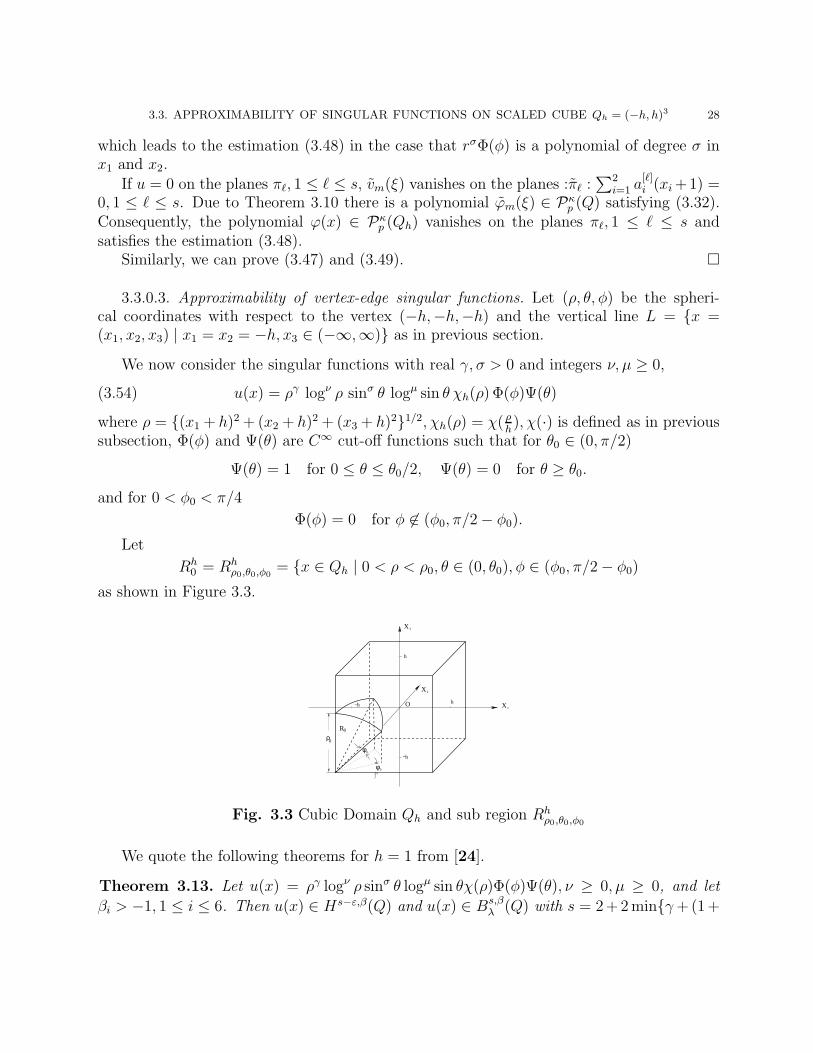
3.3.0.3. Approximability of vertex-edge singular functions. Let (ρ, θ, φ) be the spheri-cal coordinates with respect to the vertex (−h,−h,−h) and the vertical line L = x =(x1, x2, x3) | x1 = x2 = −h, x3 ∈ (−∞,∞) as in previous section.
We now consider the singular functions with real γ, σ > 0 and integers ν, µ ≥ 0,
u(x) = ργ logν ρ sinσ θ logµ sin θ χh(ρ) Φ(φ)Ψ(θ)(3.54)
where ρ = (x1 + h)2 + (x2 + h)2 + (x3 + h)21/2, χh(ρ) = χ( ρh), χ(·) is defined as in previous
subsection, Φ(φ) and Ψ(θ) are C∞ cut-off functions such that for θ0 ∈ (0, π/2)
Ψ(θ) = 1 for 0 ≤ θ ≤ θ0/2, Ψ(θ) = 0 for θ ≥ θ0.
and for 0 < φ0 < π/4
Φ(φ) = 0 for φ 6∈ (φ0, π/2 − φ0).
Let
Rh0 = Rh
ρ0,θ0,φ0= x ∈ Qh | 0 < ρ < ρ0, θ ∈ (0, θ0), φ ∈ (φ0, π/2 − φ0)
as shown in Figure 3.3.
−h
X
X
1
3
X 2
O
R0
φ
φ
0
0
ρ0
−
h
hh
Fig. 3.3 Cubic Domain Qh and sub region Rhρ0,θ0,φ0
We quote the following theorems for h = 1 from [24].
Theorem 3.13. Let u(x) = ργ logν ρ sinσ θ logµ sin θχ(ρ)Φ(φ)Ψ(θ), ν ≥ 0, µ ≥ 0, and let
βi > −1, 1 ≤ i ≤ 6. Then u(x) ∈ Hs−ε,β(Q) and u(x) ∈ Bs,βλ (Q) with s = 2+2 minγ+(1+

3.3. APPROXIMABILITY OF SINGULAR FUNCTIONS ON SCALED CUBE Qh = (−h, h)3 29
β3)/2, σ + β1 + β2, ε > 0 arbitrary, and
λ =
µ if σ < γ + (1 + β3)/2,
µ+ ν + 1/2 if σ = γ + (1 + β3)/2,
µ+ ν if σ > γ + (1 + β3)/2.
(3.55)
Theorem 3.14. Let u(x) = ργ logν ρ sinσ θ logµ sin θχ(ρ)Φ(φ)Ψ(θ), ν ≥ 0, µ ≥ 0, then thereexists ψ(x) ∈ Pκ
p (Q), 1 ≤ κ ≤ 2 with p ≥ 0 such that for βi = 0, 1 ≤ i ≤ 3, βi > −1 arbitrary,4 ≤ i ≤ 6
‖u− ψ‖L2(Q) ≤ C(1 + log(p+ 1))λ
(p+ 1)2+2minσ,γ+1/2 ‖u‖B2+2 minσ,γ+1/2,βλ (Q)
.(3.56)
Also, there exists ϕ(x) ∈ Pκp (Q), 1 ≤ κ ≤ 2 with p ≥ 0 such that for βi = −1/2, i =
1, 2, 4, 5, β3 = β6 = 0
‖u− ϕ‖H1(R0) ≤ C(1 + log(p+ 1))λ
(p+ 1)2minσ,γ+1/2 ‖u‖B1+2minσ,γ+1/2,βλ (Q)
(3.57)
and
‖u− ϕ‖C0(Q) ≤ C(1 + log(p+ 1))λ
(p+ 1)2minσ,γ+1/2−1/2‖u‖
B1+2 minσ,γ+1/2,βλ (Q)
(3.58)
with λ in (3.56)-(3.58) given in (3.55).
If u = 0 on the plane πℓ :∑2
i=1 a[ℓ]i (xi + 1) = 0, 1 ≤ ℓ ≤ s, s = 1, or 2, or 3, then
there exist ψ ∈ Pκp (Q) and ϕ ∈ Pκ
p (Q), 1 ≤ κ ≤ 2, p ≥ s such that ψ = 0 and ϕ = 0 onπℓ, 1 ≤ ℓ ≤ s, and
‖u− ψ‖L2(Q) ≤C(1 + log(p+ 1))λ
(p+ 1)2+2minσ,γ+1/2 ‖us‖B
2+2 minσ,γ+1/2,β[s]
λ (Q)
with β[s]ℓ = s, 1 ≤ ℓ ≤ 3, β
[s]ℓ > −1, 4 ≤ ℓ ≤ 6 arbitrary, and
‖u− ϕ‖H1(R0) ≤C(1 + log(p+ 1))λ
(p+ 1)2minσ,γ+1/2 ‖us‖B
1+2 minσ,γ+1/2,β[s]
λ (Q)
and
‖u− ϕ‖C0(Q) ≤C(1 + log(p+ 1))λ
(p+ 1)2minσ,γ+1/2−1/2‖us‖
B1+2 minσ,γ+1/2,β[s]
λ (Q)(3.59)
with β[s]ℓ = s− 1
2, ℓ = 1, 2, 4, 5, β
[s]ℓ = 0, ℓ = 3, 6, where
us =u(x)
∏sℓ=1
∑2i=1 a
[ℓ]i (xi + 1)
.
Due to Proposition 3.1 and Theorem 3.13, a simple scaling leads to the following theorem.

3.3. APPROXIMABILITY OF SINGULAR FUNCTIONS ON SCALED CUBE Qh = (−h, h)3 30
Theorem 3.15. Let u(x) = ργ logν ρ sinσ θ logµ sin θ χh(ρ) Φ(φ)Ψ(θ), ν ≥ 0, µ ≥ 0 as givenin (3.54), and let β = (β1, β2, β3, β4, β5, β6) with βi > −1, 1 ≤ i ≤ 6, arbitrary. Then
u ∈ Hs−ε,β(Qh) and u ∈ Bs,βλ (Qh) with s = 2 + 2 minγ + (1 + β3)/2, σ + β1 + β2, ε > 0
arbitrary, and
λ =
µ if σ < γ + (1 + β3)/2,
µ+ ν + 1/2 if σ = γ + (1 + β3)/2,
µ+ ν if σ > γ + (1 + β3)/2.
(3.60)
Proof. Let u(ξ) = u(hξ). Then for ν = µ = 0
u(ξ) = u(hξ) = hγζγ sinσ θ χ(ζ)Φ(φ)Ψ(θ) = hγw(ξ).(3.61)
and for ν ≥ 1, µ ≥ 1
u(ξ) = hγζγ(log h+ log ζ)ν sinσ θ logµ sin θ χ(ζ)Φ(φ)Ψ(θ)(3.62)
= hγζγ sinσ θ logµ sin θ χ(ζ)Φ(φ)Ψ(θ)ν∑
m=0
(ν
m
)logν−m h logm ζ
= hγν∑
m=0
(ν
m
)vm(ξ) logν−m h
where ζ =√
(ξ1 + 1)2 + (ξ2 + 1)2 + (ξ3 + 1)2, vm(ξ) = ζγ logm ζ sinσ θ logµ sin θ χ(ζ)Φ(φ)Ψ(θ)and w(ξ) = ζγ sinσ θ χ(ζ)Φ(φ)Ψ(θ). Due to Theorem 3.13, w(ξ) ∈ Hs−ε,β(Q) and vm(ξ) ∈Bs,β
λm(Q) with s = 2 + 2 minγ + (1 + β3)/2, σ + β1 + β2, ε > 0, and
λm =
µ if σ < γ + (1 + β3)/2,
µ+m+ 1/2 if σ = γ + (1 + β3)/2,
µ+m if σ > γ + (1 + β3)/2.
(3.63)
The assertions of the theorem follow immediately from Theorem 3.13 and Proposition 3.1.
By using Theorem 3.15 and the approximation property described in Theorem 3.4, weobtain the approximability of u(x).
Theorem 3.16. Let u(x) = ργ logν ρ sinσ θ logµ sin θ χh(ρ) Φ(φ)Ψ(θ), ν ≥ 0, µ ≥ 0 as givenin (3.54). Then there exists a polynomial ψ(x) in Pκ
p (Qh), 1 ≤ κ ≤ 2 with p ≥ 0 such that
‖u− ψ‖L2(Qh) ≤ Ch
32+γ
(p+ 1)2(1+minγ+1/2,σ)Fν,µ(p, h).(3.64)

3.3. APPROXIMABILITY OF SINGULAR FUNCTIONS ON SCALED CUBE Qh = (−h, h)3 31
Also there exists ϕ(x) ∈ Pκp (Qh), 1 ≤ κ ≤ 2, p ≥ 0 such that
‖u− ϕ‖H1(Rh0 ) ≤ C
h12+γ
(p+ 1)2minγ+1/2,σFν,µ(p, h).(3.65)
and
‖u− ϕ‖C0(Qh) ≤ Chγ
(p+ 1)2minγ+1/2,σ−1/2Fν,µ(p, h),(3.66)
where
Fν,µ(p, h) =
(1 + log(p+ 1))µ(1 + log p+1h
)ν−1 for integer γ,σ, ν ≥ 1, µ = 0,and ργ sinσ θΦ(φ)Ψ(θ) ∈ Pγ(Qh),
(1 + log(p+ 1))µ(1 + log p+1h
)ν , otherwise.(3.67)
and
µ =
µ if σ 6= γ + 1/2
µ+ 1/2 if σ = γ + 1/2.(3.68)
If u = 0 on the plane πℓ :∑2
i=1 a[ℓ]i (xi + 1) = 0, 1 ≤ ℓ ≤ s, s = 1, or 2, or 3, then
there exist ψ ∈ Pκp (Q) and ϕ ∈ Pκ
p (Q), 1 ≤ κ ≤ 2, p ≥ s such that ψ = 0 and ϕ = 0 onπℓ, 1 ≤ ℓ ≤ s and (3.64)-(3.66) hold.
Proof. By (3.61) for ν = µ = 0
u(ξ) = u(hξ) = hγζγ sinσ θ χ(ζ)Φ(φ)Ψ(θ) = hγw(ξ).
Then (3.64) and (3.65) with ν = µ = 0 follow from Theorem 3.14 and Proposition 3.1immediately.
Due to (3.62) for ν ≥ 1, µ ≥ 1
u(ξ) = hγζγ(log h+ log ζ)ν sinσ θ logµ sin θ χ(ζ)Φ(φ)Ψ(θ)
= hγζγ sinσ θ logµ sin θ χ(ζ)Φ(φ)Ψ(θ)
ν∑
m=0
(ν
m
)logν−m h logm ζ
= hγ
ν∑
m=0
(ν
m
)vm(ξ) logν−m h
By Theorem 3.13, vm(ξ) ∈ Bs,βλm
(Q) with s = 1 + 2 minγ + 1/2, σ, and due to Theorem
3.14, ϕm(ξ) = Πβp vm satisfies
‖vm(ξ) − ϕm(ξ)‖H1(R0)(3.69)
≤ C(p+ 1)−2minσ,γ+1/2(1 + log(p+ 1))λm‖vm(ξ)‖Bs,βλ (Q)
with λ given in (3.60).
3.3. APPROXIMABILITY OF SINGULAR FUNCTIONS ON SCALED CUBE Qh = (−h, h)3 32
If γ is not an integer, let ϕ(ξ) = hγΣνm=0
(νm
)ϕm(ξ) logν−m h, and let ϕ(x) = ϕ(x/h) =
Πβp,hu with βi = −1/3, 1 ≤ i ≤ 3, βi > −1, 4 ≤ i ≤ 6, arbitrary. Then there hold
‖u(ξ) − ϕ(ξ)‖H1(R0) ≤ Chγ
(p+ 1)2minσ,γ+1/2
ν∑
m=0
(ν
m
)(1 + log(p+ 1))λm logν−m h
≤ Chγ(1 + log(p+ 1))µ
(1 + log p+1
h
)ν
(p+ 1)2minσ,γ+1/2 ,
and
‖u(x) − ϕ(x)‖H1(Rh0 ) = h
12‖u(ξ) − ϕ(ξ)‖H1(R0) ≤ C
h12+γ(1 + log(p+ 1))µ
(p+ 1)2minσ,γ+1/2
(1 + log
p+ 1
h
)ν
with µ as given in (3.68). Thus, (3.65) for non integer γ is proved.If γ and σ are integers, µ = 0 and ργ sinσ θΦ(φ)Ψ(θ) is a polynomial of degree γ in Qh,
then v0(ξ) = ζγ sinσ θΦ(φ)Ψ(θ) is a polynomial of degree γ in Q. We rewrite (3.62) as
u(ξ) = hγ(v0(ξ) logν h+
ν∑
m=1
(ν
m
)vm(ξ) logν−m h
)= hγ
(v0(ξ) logν h + w(ξ)
).
By the argument above, there exists a polynomial ϕw(ξ) ∈ Pκp (Q), 1 ≤ κ ≤ 2 such that
‖w(ξ) − ϕw(ξ)‖H1(R0) ≤ Chγ
ν∑
m=1
(ν
m
)(1 + log(p+ 1))λm−1
(p+ 1)2minσ,γ+1/2 logν−m h
≤ Chγ(1 + log(p+ 1))µ
(1 + log p+1
h
)ν−1
(p+ 1)2minσ,γ+1/2 .
Let u0(x) = u(xh) = ργχh(ζ) sinσ θΦ(φ)Ψ(θ) logν h and w(x) = hγw(x
h). Then
u(x) = u0(x) + w(x)(3.70)
Since u0(x) is a C∞ function, there exists a polynomial ϕ0(x) ∈ Pκp (Qh), 1 ≤ κ ≤ 2 such
that
‖u0 − ϕ0‖H1(Rh0 ) ≤ C
h12+γ(1 + log(p+ 1))µ
(p+ 1)2minσ,γ+1/2
(1 + log
p+ 1
h
)ν−1
.(3.71)
Letting ϕ(x) = ϕ0(x) + ϕw(x) with ϕw(x) = hγϕw(xh). By (3.70)-(3.71), we have
‖u(x) − ϕ(x)‖H1(Rh0 ) ≤ ‖w(x) − ϕw(x)‖H1(Rh
0 ) + ‖u0 − ϕ0‖H1(Rh0 )
≤ Ch12+γ(1 + log(p+ 1))µ
(p+ 1)2minσ,γ+1/2
(1 + log
p + 1
h
)ν−1
which leads to the estimation (3.65) in the case that ργ sinσ θΦ(φ)Ψ(θ) is a polynomial.
If u = 0 on the planes πℓ, 1 ≤ ℓ ≤ s, vm(ξ) vanishes on the planes :πℓ :∑2
i=1 a[ℓ]i (xi +1) =
0, 1 ≤ ℓ ≤ s. Due to Theorem 3.14 there is a polynomial ϕm(ξ) ∈ Pκp (Q) satisfying (3.69).

3.3. APPROXIMABILITY OF SINGULAR FUNCTIONS ON SCALED CUBE Qh = (−h, h)3 33
Consequently, the polynomial ϕ(x) ∈ Pκp (Qh) vanishes on the planes πℓ, 1 ≤ ℓ ≤ s and
satisfies the estimation (3.65).Similarly, we can prove (3.64) and (3.66).

CHAPTER 4
Polynomial Extensions in Three Dimensions
4.1. Extension on a standard triangular prisms
4.1.1. Polynomial extension on a tetrahedron. For the construction of polyno-mial extensions on a triangular prism, we need quote results on the extension on a tetrahe-dron from [40]. We denote, by K, a standard tetrahedron (x1, x2, x3)|x1 ≥ 0, x2 ≥ 0, x3 ≥0, x1 + x2 + x3 ≤ 1 in R
3 shown in Fig. 4.1, and ∂K denotes the boundary of K. LetT = (x1, x2)|x1 ≥ 0, x2 ≥ 0, x1 + x2 ≤ 1 be a standard triangle in R
2, and let Γi, 1 ≤ i ≤ 3be faces of K contained in the plane xi = 0 and Γ4 be the oblique face.
1
2
3
1
1
1
O
K
Γ
Γ
ΓΓ1
3
2
4
x
x
x
Fig. 4.1 The tetrahedron K
Munoz-Sola introduced the following operators [40]
FKf(x1, x2, x3) =2
x23
∫ x1+x3
x1
dξ1
∫ x1+x2+x3−ξ1
x2
f(ξ1, ξ2)dξ2,(4.1)
and
RKf(x1, x2, x3) = (1 − x1 − x2 − x3)x1x2FK f(x1, x2, x3)(4.2)
with
f(x1, x2) =f(x1, x2)
x1x2(1 − x1 − x2).
34

4.1. EXTENSION ON A STANDARD TRIANGULAR PRISMS 35
The operator RK has the following decomposition:
RKf(x1, x2, x3) = (1 − x1 − x2 − x3)R12f(x1, x2, x3) + x2R13f(x1, x2, x3)(4.3)
+ x1R23f(x1, x2, x3),
where
R12f(x1, x2, x3) = x1x2FK f12(x1, x2, x3), f12(x1, x2) =f(x1, x2)
x1x2
,(4.4)
Ri3f(x1, x2, x3) = (1 − x1 − x2 − x3)xiFK fi3(x1, x2, x3)(4.5)
with
fi3(x1, x2) =f(x1, x2)
xi(1 − x1 − x2), i = 1, 2.
The following theorems were proved in [40].
Theorem 4.1. Let RK be the operator defined by (4.2). Then RKf(x) ∈ P1p (K) for all
f ∈ P1,0p (Γ3), and
‖RKf‖H1(K) ≤ C‖f‖H
1200(Γ3)
,(4.6)
RKf |Γ3= f, RKf |Γi= 0, i = 1, 2, 4,(4.7)
where C is a constant independent of f and p.
Theorem 4.2. For f ∈ P1p (∂K) = f ∈ C0(∂K) | f |Γi
∈ P1p (Γi), 1 ≤ i ≤ 4, there exists a
polynomial EKf ∈ P1p (K) such that EKf |∂K = f and
(4.8) ‖EKf‖H1(K) ≤ C‖f‖H1/2(∂K),
where C is a constant independent of f and p.
4.1.2. Polynomial extension on prisms from a triangular face. Let G = T ×Ibe a triangular prism with faces Γi, 1 ≤ i ≤ 5 shown in Fig. 4.2 where T = (x1, x2) |x1 ≥ 0, x2 ≥ 0, x1 + x2 ≤ 1 and I = [0, 1]. Γi, 1 ≤ i ≤ 3 are on the planes xi = 0, Γ5
is the face of G contained in the plane x3 = 1 and Γ4 is the face of G contained in theplane x1 + x2 = 1. Then Γ3 = T and Γ2 = S = I × I. By P1
p (T ) × Pp(I) we denote a setof polynomials with the sub-total degree in x1 and x2 ≤ p and with the degree ≤ p in x3.Obviously P1
p (G) ⊂ P1p (T ) ×Pp(I) ⊂ P2
p (G), it is denoted by P1.5p (G).
We shall establish polynomial extensions from the triangle T to the prism G.Since the mapping M :
x1 = x1(1 −Hx3), x2 = x2(1 −Hx3), x3 = Hx3(4.9)
maps the prism G onto a truncated tetrahedron KH = (x1, x2, x3)|x1 ≥ 0, x2 ≥ 0, H ≥x3 ≥ 0, x1 + x2 + x3 ≤ 1 with H ∈ (0, 1) shown in Fig. 4.2. Γi, i = 1, 2, 3, 4, 5 are the faces
of KH , Γ3 and Γ5 contained in the planes x3 = 0 and x3 = H , respectively, and Γi, i = 1, 2, 4are portions of the faces of the tetrahedron K. Hence, we need to construct a polynomial

4.1. EXTENSION ON A STANDARD TRIANGULAR PRISMS 36
Γ2
Γ1
Γ2
Γ3
Γ5
Γ3
Γ1
Γ4Γ4
1
1
1
O
H
1
1
1
O
Γ5 G
K
KH
1
2
3
2x
x
x
1
x
x
x3
Fig. 4.2 The prism G and truncated tetrahedron KH
extension operator RH : P1,0p (T ) → P1
p (KH)⊕P1,0
p (T ) × P1(IH) with desired properties,where IH = (0, H), which can lead to a polynomial extension from a triangular face to thewhole prism.
We now introduce polynomial lifting operator RH on KH defined by
RHf(x1, x2, x3) = RKf(x1, x2, x3) −x3
HRKf(x1, x2, H),(4.10)
where RK is the lifting operator on K given in (4.2).
Theorem 4.3. Let RH be the operator given in (4.10). Then, RHf(x) ∈ P1p (KH)
⊕P1,0p (T )×
P1(IH) for f ∈ P1,0p (T ) such that RHf(x) |Γ3
= f, RHf |Γi= 0, i = 1, 2, 4, 5, and
‖RHf‖H1(KH) ≤ C‖f‖H
1200(Γ3)
,(4.11)
where IH = (0, H) and TH = (x1, x2) | x1 ≥ 0, x2 ≥ 0, x1 + x2 ≤ 1 − H, and C is aconstant independent of f and p.
Incorporating RH and the mapping M , we construct an extension RG by
RTGf(x1, x2, x3) = RHf M = U(x1, x2, x3) − x3U(x1, x2, 1).(4.12)
where U(x1, x2, x3) = RKf M . Suppose that RKf(x1, x2, x3) =∑
i+j+k≤p aijkxi1x
j2x
k3 , then
RKf M(x1, x2, x3) = U(x1, x2, x3)
=∑
i+j+k≤p
aijkHkxi
1xj2x
k3(1 −Hx3)
i+j ∈ P1,0p (T ) ×Pp(I).
andx3
HRKf(x1, x2, H) M = x3U(x1, x2, 1) ∈ P1,0
p (T ) ×P1(I).
Therefore RTGf(x1, x2, x3) = RHf M ∈ P1,0
p (T ) × Pp(I) if f ∈ P1,0p (T ). We are able to
establish the polynomial extension from a triangular face to a prism.

4.1. EXTENSION ON A STANDARD TRIANGULAR PRISMS 37
Theorem 4.4. Let RTG be the extension defined in (4.12). Then RT
Gf ∈ P1,0p (T )×Pp(I) for
f ∈ P1,0p (T ) , RT
Gf |Γ3= f and vanishes on ∂G\Γ3, and
‖RTGf‖H1(G) ≤ C‖f‖
H1200(Γ3)
,(4.13)
where C is a constant independent of f and p.
Proof. Obviously, RTG : P1,0
p (T ) → P1,0p (T )×Pp(I), andRT
Gf = f for all f ∈ P1,0p (T ), RT
Gf |Γi=
0, i = 1, 2, 4, 5. Since the mapping M is trilinear,
‖RTGf‖H1(G) ≤ C‖RHf‖H1(KH).
Then (4.13) follows from (4.11) easily.
It remained to prove Theorem 4.3. To this end, we need the following lemmas.
Lemma 4.5. For 0 < h < a and any function g ∈ L2(0, a), it holds that∫ a−h
0
∣∣∣1h
∫ x+h
x
g(ξ)dξ∣∣∣2
dx ≤∫ a
0
|g(x)|2dx.(4.14)
Also there hold
(4.15)
∫ a−h
0
∣∣∣1h
∫ x+h
x
g(ξ)dξ∣∣∣2
dx ≤ 1
h
∫ a
0
x|g(x)|2dx
and
(4.16)
∫ a−h
0
∣∣∣1h
∫ x+h
x
g(ξ)dξ∣∣∣2
dx ≤ 1
h
∫ a
0
(a− x)|g(x)|2dx.
Proof. By Schwarz inequality, we have∫ a−h
0
∣∣∣1h
∫ x+h
x
g(ξ)dξ∣∣∣2
dx ≤∫ a−h
0
∣∣∣1h
∫ x+h
x
|g(ξ)|dξ∣∣∣2
dx ≤∫ a−h
0
dx
∫ x+h
x
|g(ξ)|2h
dξ.
ξ=x
Case 1. 0 < h < a/2 Case 2. 0 < a/2 < h < a
ξ
O
ξ=x
ξ=x+hξ
O
h
ξ=x+h
a−h a−h
a
a
ha−h a−h
XX
Fig. 4.3 Case 1 and Case 2

4.1. EXTENSION ON A STANDARD TRIANGULAR PRISMS 38
• Case 1 : 0 < h ≤ a/2. There holds∫ a−h
0
∣∣∣1h
∫ x+h
x
g(ξ)dξ∣∣∣2
dx ≤∫ a−h
0
dx
∫ x+h
x
|g(ξ)|2h
dξ
=
∫ h
0
dξ
∫ ξ
0
|g(ξ)|2h
dx+
∫ a−h
h
dξ
∫ ξ
ξ−h
|g(ξ)|2h
dx+
∫ a
a−h
dξ
∫ a−h
ξ−h
|g(ξ)|2h
dx
=
∫ h
0
ξ|g(ξ)|2h
dξ +
∫ a−h
h
h|g(ξ)|2h
dξ +
∫ a
a−h
(a− ξ)|g(ξ)|2h
dξ.
Hence, we have∫ a−h
0
∣∣∣1h
∫ x+h
x
g(ξ)dξ∣∣∣2
dx ≤∫ a
0
|g(ξ)|2dξ
and∫ a−h
0
∣∣∣1h
∫ x+h
x
g(ξ)dξ∣∣∣2
dx ≤ 1
h
∫ a
0
ξ|g(ξ)|2dξ.
• Case 2 : a/2 < h < a. Similarly, there holds∫ a−h
0
∣∣∣1h
∫ x+h
x
g(ξ)dξ∣∣∣2
dx ≤∫ a−h
0
dx
∫ x+h
x
|g(ξ)|2h
dξ
=
∫ a−h
0
dξ
∫ ξ
0
|g(ξ)|2h
dx+
∫ h
a−h
dξ
∫ a−h
0
|g(ξ)|2h
dx+
∫ a
h
dξ
∫ a−h
ξ−h
|g(ξ)|2h
dx
=
∫ a−h
0
ξ|g(ξ)|2h
dξ +
∫ h
a−h
(a− h)|g(ξ)|2h
dξ +
∫ a
h
(a− ξ)|g(ξ)|2h
dξ,
which implies∫ a−h
0
∣∣∣1h
∫ x+h
x
g(ξ)dξ∣∣∣2
dx ≤∫ a
0
|g(ξ)|2dξ
and∫ a−h
0
∣∣∣1h
∫ x+h
x
g(ξ)dξ∣∣∣2
dx ≤ 1
h
∫ a
0
ξ|g(ξ)|2dξ.
Therefore we always have (4.14) and (4.15) for 0 < h ≤ a/2 or a/2 < h < a.
Letting η = a− ξ and x = a− h− x and using (4.15) we obtain∫ a−h
0
∣∣∣1h
∫ x+h
x
g(ξ)dξ∣∣∣2
dx =
∫ a−h
0
∣∣∣1h
∫ x+h
x
g(a− η)dη∣∣∣2
dx
≤ 1
h
∫ a
0
x|g(a− x)|2dx =1
h
∫ a
0
(a− z)|g(z)|2dz,
which yields (4.16).
4.1. EXTENSION ON A STANDARD TRIANGULAR PRISMS 39
Lemma 4.6. Let R12(x1, x2, H) and Ri3(x1, x2, H) be the operators given in (4.4) and (4.5)with x3 = H. Then
‖R12f(x1, x2, H)‖L2(KH) ≤ C‖(x1x2)12 f(x1, x2)‖L2(T ),(4.17)
and for i = 1, 2
‖Ri3f(x1, x2, H)‖L2(KH) ≤ C‖x12i (1 − x1 − x2)
12f(x1, x2)‖L2(T ),(4.18)
where C is a constant independent of f .
Proof. Note that
‖R12f(x1, x2, H)‖2L2(KH) ≤
4
H2
∫ H
0
dx3
∫ 1−x3
0
dx2
∫ 1−x2−x3
0
∣∣∣ 1
H
∫ x1+H
x1
g1(ξ1)dξ1
∣∣∣2
dx1
with g1(ξ1) =
∫ x2+H
x2
|f(ξ1, ξ2)|dξ2. Hereafter f denotes the extension of f by zero outside
T . We apply here Lemma 4.5 to g1(ξ1) with a = 1− x2 − x3, h = H, x = x1, ξ = ξ1, then weget
∫ 1−x2−x3
0
( 1
H
∫ x1+H
x1
g(ξ1)dξ1
)2
dx1 ≤1
H
∫ 1−x2−x3+H
0
x1|g1(x1)|2dx1,
which implies
∫ 1−x3
0
dx2
∫ 1−x2−x3
0
∣∣∣ 1
H
∫ x1+H
x1
g1(ξ1)dξ1
∣∣∣2
dx1(4.19)
≤ 1
H
∫ 1−x3
0
dx2
∫ 1−x2−x3+H
0
x1
∣∣∣∫ x2+H
x2
|f(x1, ξ2)|dξ2∣∣∣2
dx1
= H∫ H
0
x1dx1
∫ 1−x3
0
∣∣∣ 1
H
∫ x2+H
x2
|f(x1, ξ2)|dξ2∣∣∣2
dx2
+
∫ 1−x3+H
H
x1dx1
∫ 1−x1−x3+H
0
∣∣∣ 1
H
∫ x2+H
x2
|f(x1, ξ2)|dξ2∣∣∣2
dx2
.
Applying Lemma 4.5 again, we have
∫ 1−x3
0
∣∣∣ 1
H
∫ x2+H
x2
|f(x1, ξ2)|dξ2∣∣∣2
dx2 ≤1
H
∫ 1−x3+H
0
x2|f(x1, x2)|2dx2,
and∫ 1−x1−x3+H
0
∣∣∣ 1
H
∫ x2+H
x2
|f(x1, ξ2)|dξ2∣∣∣2
dx2 ≤ 1
H
∫ 1−x1−x3+2H
0
x2|f(x1, x2)|2dx2,

4.1. EXTENSION ON A STANDARD TRIANGULAR PRISMS 40
which together with (4.19) yields∫ 1−x3
0
dx2
∫ 1−x2−x3
0
( 1
H
∫ x1+H
x1
dξ1
∫ x2+H
x2
|f(ξ1, ξ2)|dξ2)2
dx1
≤(∫ H
0
dx1
∫ 1+H
0
+
∫ 1−x3+H
H
dx1
∫ 1−x1+2H
0
)x2x1|f(x1, x2)|2dx2
≤(∫ H
0
dx1
∫ 1+H
0
+
∫ 1+H
H
dx1
∫ 1−x1+2H
0
)x2x1|f(x1, x2)|2dx2 ≤ 2‖(x1x2)
12 f‖2
L2(T ).
Therefore (4.17) follows immediately.Let Q1 be the mapping:
x1 = x2, x2 = 1 − x1 − x2 − x3, x3 = x3,(4.20)
which maps KH onto itself, and let W1 be the mapping:
ξ1 = ξ2, ξ2 = 1 − ξ1 − ξ2,(4.21)
which maps T onto itself. Then f(ξ1, ξ2) = f(ξ1, ξ2)W1 = f(ξ2, 1−ξ1−ξ2) andR12f(x1, x2, H) =R13f(x1, x2, x3) Q1 |x3=H . Therefore
‖R13f(x1, x2, H)‖L2(KH) ≤ ‖R12f(x1, x2, H)‖L2(KH) ≤ C‖(ξ1ξ2)12 f‖L2(T )
≤ C‖ξ121 (1 − ξ1 − ξ2)
12f‖L2(T ).
For R23f , we introduce mapping Q2 and W2:
Q2 : x1 = 1 − x1 − x2 − x3, x2 = x1, x3 = x3,(4.22)
which maps KH onto itself, and
W2 : ξ1 = 1 − ξ1 − ξ2, ξ2 = ξ1,(4.23)
which maps T onto itself. Similarly
‖R23f(x1, x2, H)‖L2(KH) ≤ ‖R12f(x1, x2, H)‖L2(KH) ≤ C‖(ξ1ξ2)12 f‖L2(T )
≤ C‖ξ122 (1 − ξ1 − ξ2)
12f‖L2(T ).
Lemma 4.7. Let R12(x1, x2, H) and Ri3(x1, x2, H) be the operators given in (4.4) and (4.5)with x3 = H. Then for i = 1, 2
∥∥∥∂R12f(x1, x2, H)
∂xi
∥∥∥L2(KH)
≤ C‖x−12
i f‖L2(T ),(4.24)
and t = 1, 2∥∥∥∂Ri3f(x1, x2, H)
∂xt
∥∥∥L2(KH)
≤ C(‖x−
12
t f‖L2(T ) + ‖(1 − x1 − x2)− 1
2f‖L2(T )
),(4.25)
where C is a constant independent of f .

4.1. EXTENSION ON A STANDARD TRIANGULAR PRISMS 41
Proof. Note that
∂R12f(x1, x2, H)
∂x1
=2x2
H2
∫ x1+H
x1
dξ1
∫ x1+x2+H−ξ1
x2
f(ξ1, ξ2)
ξ1ξ2dξ2
−2x2
H2
∫ x2+H
x2
f(x1, ξ2)
ξ2dξ2 +
2x1x2
H2
∫ x1+H
x1
f(ξ1, x1 + x2 +H − ξ1)
ξ1(x1 + x2 +H − ξ1)dξ1
and
∣∣∣∂R12f(x1, x2, H)
∂x1
∣∣∣ ≤ I1 + I2 + I3,(4.26)
where
I1 =2
H2
∫ x1+H
x1
dξ1
∫ x2+H
x2
|f(ξ1, ξ2)|ξ1
dξ2, I2 =2
H2
∫ x2+H
x2
|f(x1, ξ2)|dξ2
I3 =2
H2
∫ x1+H
x1
|f(ξ1, x1 + x2 +H − ξ1)|dξ1.
Note that
‖I1‖2L2(KH) =
4
H2
∫ H
0
dx3
∫ 1−x3
0
dx2
∫ 1−x2−x3
0
( 1
H
∫ x1+H
x1
g1(ξ1)dξ1
)2
dx1
with g1(ξ1) =
∫ x2+H
x2
|f(ξ1, ξ2)|ξ1
dξ2. Applying Lemma 4.5 to g1(ξ1) with a = 1−x2−x3, h =
H, x = x1, ξ = ξ1, we have
∫ 1−x2−x3
0
∣∣∣ 1
H
∫ x1+H
x1
g1(ξ1)dξ1
∣∣∣2
dx1 ≤1
H
∫ 1−x2−x3+H
0
x1
∣∣∣∫ x2+H
x2
f(x1, ξ2)
x1dξ2
∣∣∣2
dx1,
which implies
∫ 1−x3
0
dx2
∫ 1−x2−x3
0
∣∣∣ 1
H
∫ x1+H
x1
g1(ξ1)dξ1
∣∣∣2
dx1
≤ 1
H
∫ 1−x3
0
dx2
∫ 1−x2−x3+H
0
1
x1
∣∣∣∫ x2+H
x2
f(x1, ξ2)dξ2
∣∣∣2
dx1
≤ H∫ H
0
1
x1dx1
∫ 1−x3
0
∣∣∣ 1
H
∫ x2+H
x2
f(x1, ξ2)dξ2
∣∣∣2
dx2
+
∫ 1−x3+H
H
1
x1
dx1
∫ 1−x1−x3+H
0
∣∣∣ 1
H
∫ x2+H
x2
f(x1, ξ2)dξ2
∣∣∣2
dx2
.

4.1. EXTENSION ON A STANDARD TRIANGULAR PRISMS 42
Applying Lemma 4.5 again to the function g2(ξ2) = f(x1, ξ2), we have
‖I1‖2L2(KH) ≤ 4
H2
∫ H
0
dx3
∫ H
0
1
x1dx1
∫ 1−x3+H
0
|f(x1, x2)|2dx2(4.27)
+4
H2
∫ H
0
dx3
∫ 1−x3+H
H
1
x1dx1
∫ 1−x1−x3+2H
0
|f(x1, x2)|2dx2
≤ 4
H
(∫ H
0
dx1
∫ 1+H
0
+
∫ 1+H
H
dx1
∫ 1−x1+2H
0
) |f(x1, x2)|2x1
dx2
≤ 8
H‖x1
− 12f‖2
L2(T ).
Similarly we have by Lemma 4.5,
‖I2‖2L2(KH) =
4
H2
∫ H
0
dx3
∫ 1−x3
0
dx1
∫ 1−x1−x3
0
∣∣∣ 1
H
∫ x2+H
x2
|f(x1, ξ2)|dξ2∣∣∣2
dx2(4.28)
≤ 4
H3
∫ H
0
dx3
∫ 1−x3
0
dx1
∫ 1−x1−x3+H
0
x2|f(x1, x2)|2dx2
≤ 4
H3
∫ H
0
dx3
∫ 1
0
dx1
∫ 1−x1+H
0
x2|f(x1, x2)|2dx2 =4
H2‖x
122 f‖2
L2(T ),
and
‖I3‖2L2(KH) =
4
H2
∫ H
0
dx3
∫ 1−x3
0
dx2
∫ 1−x2−x3
0
∣∣∣ 1
H
∫ x1+H
x1
|f(ξ1, x1 + x2 +H − ξ1)|dξ1∣∣∣2
dx1
≤ 4
H3
∫ H
0
dx3
∫ 1−x3
0
dx2
∫ 1−x2−x3+H
0
x1|f(x1, x2 +H)|2dx1
≤ 4
H3
∫ H
0
dx3
∫ 1
0
dx2
∫ 1−x2+H
0
x1|f(x1, x2 +H)|2dx1
=4
H2
∫ 1
0
dx2
∫ 1−x2+H
0
x1|f(x1, x2 +H)|2dx1.
Letting z = x2 +H , we have
4
H2
∫ 1
0
dx2
∫ 1−x2+H
0
x1|f(x1, x2 +H)|2dx1 =4
H2
∫ 1+H
H
dz
∫ 1−z+2H
0
x1|f(x1, z)|2dx1
=4
H2
∫ 1
H
dz
∫ 1−z
0
x1|f(x1, z)|2dx1 ≤4
H2‖x
121 f‖2
L2(T ),
which implies
‖I3‖2L2(KH) ≤
4
H2‖x
121 f‖2
L2(T ).(4.29)

4.1. EXTENSION ON A STANDARD TRIANGULAR PRISMS 43
Combining (4.26)-(4.29), we have
∥∥∥∂R12f(x1, x2, H)
∂x1
∥∥∥L2(KH)
≤ C‖x−12
1 f‖L2(T ).
Similarly, we can prove
∥∥∥∂R12f(x1, x2, H)
∂x2
∥∥∥L2(KH)
≤ C‖x−12
2 f‖L2(T ).
Let Qi and Wi (i=1,2) be the mapping as defined in (4.20)-(4.23). Then, for t = 1, 2,
∥∥∥∂R13f(x1, x2, H)
∂xt
∥∥∥L2(KH)
≤∑
i=1,2
∥∥∥∂R12f(x1, x2, H)
∂xi
∥∥∥L2(KH)
≤ C∑
i=1,2
‖ξ−12
i f‖L2(T )
≤ C(‖ξ−12
1 f‖L2(T ) + ‖(1 − ξ1 − ξ2)− 1
2 f‖L2(T )).
Similarly, we have for t = 1, 2
∥∥∥∂R23f(x1, x2, H)
∂xt
∥∥∥L2(KH)
≤∑
i=1,2
∥∥∥∂R12f(x1, x2, H)
∂xi
∥∥∥L2(KH)
≤ C∑
i=1,2
‖ξ−12
i f‖L2(T )
≤ C(‖ξ−12
2 f‖L2(T ) + ‖(1 − ξ1 − ξ2)− 1
2 f‖L2(T )).
Proof of Theorem 4.3 Obviously, RHf(x) ∈ P1p (KH)
⊕P1,0p (T )×P1(IH) for f ∈ P1,0
p (T ).Due to (4.10), we have
‖RHf(x1, x2, x3)‖H1(KH)(4.30)
≤ ‖RKf(x1, x2, x3)‖H1(KH) +∥∥∥x3
HRKf(x1, x2, H)
∥∥∥H1(KH)
.
By Theorem 4.1, there holds
‖RKf(x1, x2, x3)‖H1(KH) ≤ ‖RKf(x1, x2, x3)‖H1(K) ≤ C‖f(x1, x2)‖H
1200(T )
,(4.31)
and by (4.3) and Lemma 4.6- Lemma 4.7, it holds that∥∥∥x3
HRKf(x1, x2, H)
∥∥∥H1(KH)
≤ C(‖R12f(x1, x2, H)‖H1(KH) +∑
i=1,2
‖Ri3f(x1, x2, H)‖H1(KH))
≤ C(‖f‖H
12 (T )
+∑
i=1,2
‖x−12
i f‖L2(T ) + ‖(1 − x1 − x2)− 1
2 f‖L2(T )) ≤ C‖f‖H
1200(T )
,
which together with (4.30)-(4.31) leads to (4.11) immediately.

4.1. EXTENSION ON A STANDARD TRIANGULAR PRISMS 44
4.1.3. Polynomial extension on prisms from a square face. We shall constructa polynomial extension on prisms from a square face S = x = (x1, x2, x3) | 0 ≤ x1, x3 ≤1, which is as important as the extension from a triangular face for error analysis andpreconditioning of high-order finite element methods in three dimensions [25].
Lemma 4.8. Let T = (x1, x2)|0 < x2 < 1 − x1, 0 ≤ x1 < 1 be the standard triangle andI = (0, 1). Then there is a polynomial extension operator R∗
T : H10 (I) → H1(T ) such that
R∗Tf ∈ P1
p (T ) if f(x1) ∈ P0p (I), and
R∗Tf |I = f(x1), R
∗T f |∂T\I = 0,(4.32)
‖R∗Tf‖Ht(T ) ≤ C
(pt− 3
2‖f‖H1(I) + pt− 12‖f‖L2(I)
), t = 0, 1.(4.33)
with C independent of f and p.
Proof. Let ψ(x2) = (1 − x2)p. Then for t ≥ 0
‖ψ‖Ht(I) ≤ Cpt− 12 .(4.34)
We introduce a function Ψ ∈ P12p+1(T ) by
Ψ(x1, x2) = ψ(x2)((1 − x1 − x2)f(x1) + x1f(x1 + x2)
).
Then Ψ(x1, 0) = f(x1),Ψ(1, x2) = Ψ(x1, 1 − x1) = 0, and
(4.35) ‖Ψ‖L2(T ) ≤ Cp−12‖f‖L2(I),
(4.36) ‖Ψ‖H1(T ) ≤ C(p−
12‖f‖H1(I) + p
12‖f‖L2(I)
).
By the lifting theorem on the triangle T [35], there exists a lifting operator RT : H1200(I) →
H1(T )
RTf =x1(1 − x1 − x2)
x22
∫ x1+x2
x1
f(ξ)
ξ(1 − ξ)dξ
such that RTf ∈ P1p (T ), RTf |I= f and RTf |∂T\I= 0, and
‖RT f‖H1(T ) ≤ C‖f‖H
1200(I)
,
which implies that RT satisfies (4.33) with t = 1. Unfortunately, the extension does not givea precise information on ‖RTf‖L2(T ), and the desired estimation (4.33) with t = 0 may notbe true for RT . Therefore we have to construct a new extension operator R∗
T .Note that Ψ − RT f = 0 on ∂T . By ΠT we denote the orthogonal projection operator:
H10 (T ) → P1,0
p (T ), and let
wp = RT f + ΠT (Ψ −RT f).
Then wp(x1, 0) = f(x1) and wp(1, x2) = wp(x1, 1 − x1) = 0, and
Ψ − wp =(I − ΠT
)(Ψ − RTf).(4.37)
4.1. EXTENSION ON A STANDARD TRIANGULAR PRISMS 45
Due to the continuity of operator RT and a trace theorem, we obtain
‖wp‖H1(T ) ≤ ‖Ψ‖H1(T ) + ‖Ψ − wp‖H1(T ) ≤ ‖Ψ‖H1(T ) + ‖Ψ − RTf‖H1(T )(4.38)
≤ 2‖Ψ‖H1(T ) + ‖RT f‖H1(T ) ≤ C(‖Ψ‖H1(T ) + ‖f‖H
1200(I)
)
≤ C(‖Ψ‖H1(T ) + ‖Ψ‖H
12 (∂T )
) ≤ C‖Ψ‖H1(T ).
Let R∗Tf = wp. Then (4.36) and (4.38) leads to (4.32) and (4.33) with t = 1. Note that
ΠT (Ψ − RTf) is the finite element solution in P1,0p (T ) for the the boundary value problem:
−∆u + u = f in T
u |∂T = 0
with f = −∆(Ψ −RT f) + Ψ − RTf . By the Nitsche’s trick, we have
‖(I − ΠT
)(Ψ − RTf)‖L2(T ) ≤ Cp−1‖
(I − ΠT
)(Ψ −RT f)‖H1(T ) ≤ Cp−1‖Ψ‖H1(T ),
which implies
‖Ψ − wp‖L2(T ) = ‖(I − ΠT
)(Ψ − RTf)‖L2(T ) ≤ Cp−1‖Ψ‖H1(T ).(4.39)
Combining (4.39) and (4.36) we have (4.33) for t = 0.
We construct a polynomial extension from a square face to the prism G with help of theextension R∗
T in triangle T :
RSGf(x1, x2, x3) = R∗
Tf(·, x3)(4.40)
Theorem 4.9. Let Γ2 = S be a square face of the prism G as shown in Fig. 4.2, and let RSG
be the extension operator defined as in (4.40). Then RSGf ∈ P1
p (T )×Pp(I) for f ∈ P2,0p (Γ2),
and
RSGf = f on Γ2, RS
Gf = 0 on ∂G\Γ2,(4.41)
‖RSGf‖H1(G) ≤ C
(p−
32 |fx3|H1(Γ2) + p−
12 |f |H1(Γ2) + p
12‖f‖L2(Γ2)
),(4.42)
‖RSGf‖L2(G) ≤ C
(p−
32‖f‖H1(Γ2) + p−
12‖f‖L2(Γ2)
).(4.43)
Proof. Obviously, RSGf ∈ P1
p (T ) × Pp(I) and (4.41) holds. Due to (4.40)
‖RSGf‖2
L2(G) =
∫ 1
0
(∫
T
| RSGf |2 dx1dx2
)dx3 ≤
∫ 1
0
‖R∗Tf‖2
L2(T )dx3
≤ C
∫ 1
0
(p−3‖f(·, x3)‖2
H1(I) + p−1‖f(·, x3)‖2L2(I)
)dx3
≤ C(p−3‖f‖2
H1(S) + p−1‖f‖2L2(S)
)
which leads to (4.43).

4.2. EXTENSION ON A STANDARD PYRAMID 46
Applying (4.40) to f(x1, x3) and fx3(x1, x3), respectively, we have
|RSGf |2H1(G) ≤
∫ 1
0
(|R∗
Tf |2H1(T ) + |R∗Tfx3|2L2(T )
)dx3
≤ C
∫ 1
0
(p−1‖f‖2
H1(I) + p1‖f‖2L2(I) + p−3‖fx3‖2
L2(I)
)dx3
≤ C(p−3|fx3|2H1(S) + p−1|f |2H1(S) + p‖f‖2
L2(S)
),
which implies (4.42).
Remark 4.1. It is an open problem whether there exists a polynomial extension operator RSG
such that
‖RSGf‖H1(G) ≤ C‖f‖
H1/200 (Γ2)
.(4.44)
Although (4.42) is not strong as (4.44), it gives the dependence of ‖RSGf‖H1(G) on ‖f‖Ht(S), t =
2, 1, 0 furnished precisely with a weight p−3/2, p−1/2 and p1/2, respectively. This estimation issufficient while applying the extension to a pair of elements sharing a common square facefor constructing a continuous piecewise polynomial in P1.5
p (G). Hence, Theorem 4.9 plays animportant role in error analysis for the p and h-p versions of finite element method in threedimensions on meshes containing triangular prism elements.
4.2. Extension on a standard pyramid
We denote, by Λ, a standard pyramid (x1, x2, x3) | 0 ≤ x1 ≤ 1, 0 ≤ x2 ≤ 1, 0 ≤x3 ≤ 1, x1 + x3 ≤ 1, x2 + x3 ≤ 1in R
3 shown in Fig. 4.4 . Let Γi, 1 ≤ i ≤ 3 be thefaces of Λ contained in the plane xi = 0 and Γi, i = 4, 5 be the oblique faces, and letS = (x1, x2) | 0 ≤ x1 ≤ 1, 0 ≤ x2 ≤ 1 be a square in R
2. Obviously, Γ3 = S. For f inL1(S), we introduce an extension operator FΛf on Λ by
(4.1) FΛf(x1, x2, x3) =1
x23
∫ x1+x3
x1
dξ1
∫ x2+x3
x2
f(ξ1, ξ2)dξ2.
It is easy to verify that if f ∈ P1p (S), then FΛf ∈ P1
p (Λ) and it holds that FΛf(x1, x2, 0) =f(x1, x2) and we have the following theorem.
Theorem 4.10. Let FΛ be the operator defined by (4.1). Then for any f in H12 (S), there
hold
‖FΛf‖L2(Λ) ≤ C‖f‖L2(S)(4.2)
and
‖FΛf‖H1(Λ) ≤ C‖f‖H
12 (S)
.(4.3)
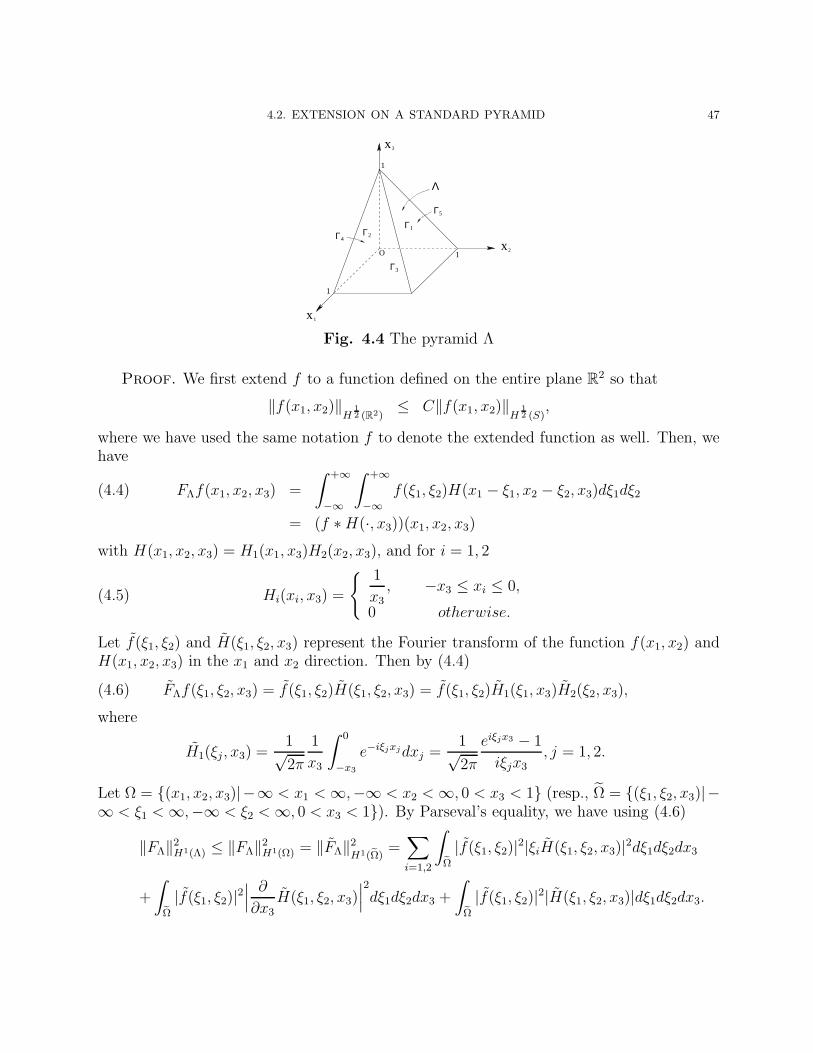
4.2. EXTENSION ON A STANDARD PYRAMID 47
2
3
1
1
1
O
Γ Γ
Γ3
ΓΓ
12
4
5
1x
x
x
Λ
Fig. 4.4 The pyramid Λ
Proof. We first extend f to a function defined on the entire plane R2 so that
‖f(x1, x2)‖H12 (R2)
≤ C‖f(x1, x2)‖H12 (S)
,
where we have used the same notation f to denote the extended function as well. Then, wehave
FΛf(x1, x2, x3) =
∫ +∞
−∞
∫ +∞
−∞f(ξ1, ξ2)H(x1 − ξ1, x2 − ξ2, x3)dξ1dξ2(4.4)
= (f ∗H(·, x3))(x1, x2, x3)
with H(x1, x2, x3) = H1(x1, x3)H2(x2, x3), and for i = 1, 2
Hi(xi, x3) =
1
x3, −x3 ≤ xi ≤ 0,
0 otherwise.(4.5)
Let f(ξ1, ξ2) and H(ξ1, ξ2, x3) represent the Fourier transform of the function f(x1, x2) andH(x1, x2, x3) in the x1 and x2 direction. Then by (4.4)
FΛf(ξ1, ξ2, x3) = f(ξ1, ξ2)H(ξ1, ξ2, x3) = f(ξ1, ξ2)H1(ξ1, x3)H2(ξ2, x3),(4.6)
where
H1(ξj, x3) =1√2π
1
x3
∫ 0
−x3
e−iξjxjdxj =1√2π
eiξjx3 − 1
iξjx3, j = 1, 2.
Let Ω = (x1, x2, x3)|−∞ < x1 <∞,−∞ < x2 <∞, 0 < x3 < 1 (resp., Ω = (ξ1, ξ2, x3)|−∞ < ξ1 <∞,−∞ < ξ2 <∞, 0 < x3 < 1). By Parseval’s equality, we have using (4.6)
‖FΛ‖2H1(Λ) ≤ ‖FΛ‖2
H1(Ω) = ‖FΛ‖2H1(Ω)
=∑
i=1,2
∫
Ω
|f(ξ1, ξ2)|2|ξiH(ξ1, ξ2, x3)|2dξ1dξ2dx3
+
∫
Ω
|f(ξ1, ξ2)|2∣∣∣ ∂
∂x3
H(ξ1, ξ2, x3)∣∣∣2
dξ1dξ2dx3 +
∫
Ω
|f(ξ1, ξ2)|2|H(ξ1, ξ2, x3)|dξ1dξ2dx3.

4.2. EXTENSION ON A STANDARD PYRAMID 48
Noting that |Hi(ξi, x3)| ≤ C for i = 1, 2, we have∫
Ω
|f(ξ1, ξ2)|2|H(ξ1, ξ2, x3)|2dξ1dξ2dx3 ≤ C
∫
R2
|f(ξ1, ξ2)|2dξ1dξ2 ≤ C‖f‖2L2(R2),(4.7)
which implies (4.2).
Letting uj = x3|ξj| for j = 1, 2, we obtain
∫ 1
0
|Hj(ξj, x3)|2dx3 =1
2π|ξj|
∫ |ξj |
0
∣∣∣eiuj − 1
iuj
∣∣∣2
duj =1
π|ξj|
∫ |ξj |
0
1 − cosuj
u2j
duj ≤C
|ξj|,
which yields for j = 1, 2∫
Ω
|f |2|ξjH(ξ1, ξ2, x3)|2dξ1dξ2dx3 ≤ C
∫
R2
|ξj||f(ξ1, ξ2)|2dξ1dξ2(4.8)
≤ C‖f‖2
H12 (R2)
≤ C‖f‖2
H12 (S)
.
Note that
∂
∂x3H(ξ1, ξ2, x3) =
1
2π
( iξ1x3eiξ1x3 − eiξ1x3 + 1
iξ1x23
H(ξ2, x3) +iξ2x3e
iξ2x3 − eiξ2x3 + 1
iξ2x23
H(ξ1, x3))
and
∣∣∣ ∂
∂x3H(ξ1, ξ2, x3)
∣∣∣2
≤ C
2π
2∑
j=1
|ξj|22(1 − cosuj) + u2
j − 2uj sin uj
u4j
,
which imply
∫ 1
0
∣∣∣ ∂
∂x3
H(ξ1, ξ2, x3)∣∣∣2
dx3 ≤C
2π
2∑
j=1
∫ |ξj |
0
|ξj|2(1 − cosuj) + u2
j − 2uj sin uj
u4j
duj ≤ C(|ξ1| + |ξ2|)
and∫
Ω
|f(ξ1, ξ2)|2∣∣∣ ∂
∂x3H(ξ1, ξ2, x3)
∣∣∣2
dξ1dξ2dx3 ≤ C
∫
R2
(|ξ1| + |ξ2|)|f(ξ1, ξ2)|2dξ1dξ2(4.9)
≤ C‖f‖2
H12 (R2)
≤ C‖f‖2
H12 (S)
.
A combination of (4.7)-(4.9) leads to (4.3).
Remark 4.2. Theorem 4.10 can be generalized to high order, FΛf realizes a continuous map-ping Hm− 1
2 (S) → Hm(Λ) for m ≥ 1.
We now introduce an extension operator RΛ : H1200(S) → H1(Λ)
RΛf(x1, x2, x3) = x1x2(1 − x1 − x3)(1 − x2 − x3)FΛf(x1, x2, x3)(4.10)

4.2. EXTENSION ON A STANDARD PYRAMID 49
with f(x1, x2) = f(x1,x2)x1x2(1−x1)(1−x2)
. Due to the identity
1
x1x2(1 − x1)(1 − x2)
=1
2
1
x1x2(1 − x1)+
1
x1x2(1 − x2)+
1
x1(1 − x1)(1 − x2)+
1
x2(1 − x1)(1 − x2)
,
RΛ has the decomposition:
RΛf(x1, x2, x3) =1
2x2R145f(x1, x2, x3) + x1R245f(x1, x2, x3)(4.11)
+(1 − x2 − x3)R124f(x1, x2, x3) + (1 − x1 − x3)R125f(x1, x2, x3) ,where
Ri45f(x1, x2, x3) = xi(1 − x1 − x3)(1 − x2 − x3)FΛfi45(x1, x2, x3)(4.12)
with fi45(x1, x2) = f(x1,x2)xi(1−x1)(1−x2)
, i = 1, 2, and for s = 4, 5
R12sf(x1, x2, x3) = x1x2(1 − xs−3 − x3)FΛf12s(x1, x2, x3),(4.13)
f12s(x1, x2) =f(x1, x2)
x1x2(1 − xs−3).
We shall prove the desired polynomial extension theorem on the pyramid Λ.
Theorem 4.11. Let RΛ be the operator as given in (4.10). Then RΛf(x1, x2, x3) ∈ P1p (Λ)
for all f ∈ P1,0p (S), and
‖RΛf(x1, x2, x3)‖H1(Λ) ≤ C‖f(x1, x2)‖H
1200(S)
,(4.14)
RΛf |Γ3= f, RΛf |Γi= 0, i = 1, 2, 4, 5,(4.15)
where C is a constant independent of f and p.
In order to prove this theorem, we need following lemmas.
Lemma 4.12. Let
g1 =1
x23
∫ x2+x3
x2
|f(x1 + x3, ξ2) − f(x1, ξ2)|dξ2(4.16)
and
g2 =1
x23
∫ x1+x3
x1
|f(ξ1, x2 + x3) − f(ξ1, x2)|dξ1.(4.17)
Then there holds
‖gs‖L2(Λ) ≤ C‖f‖H
12 (S)
, s = 1, 2.(4.18)
4.2. EXTENSION ON A STANDARD PYRAMID 50
Proof. We first extend f to square S2 = (x1, x2) | 0 ≤ x1 ≤ 2, 0 ≤ x2 ≤ 2 and
denoted the extension of f by f such that
‖f‖H
12 (S2)
≤ C‖f‖H
12 (S)
.
Let Q = (x1, x2, x3) | 0 ≤ x1 ≤ 1, 0 ≤ x3 ≤ 1, 0 ≤ x2 ≤ 1 − x3 be a prism containing Λ,there holds
‖g1‖2L2(Λ) ≤
∥∥∥ 1
x23
∫ x2+x3
x2
| f(x1 + x3, ξ2) − f(x1, ξ2) | dξ2∥∥∥
2
L2(Q)
≤∫ 1
0
dx1
∫ 1
0
dx2
∫ 1−x2
0
∣∣∣ 1
x3
∫ x2+x3
x2
| f(x1 + x3, ξ2) − f(x1, ξ2) |x3
dξ2
∣∣∣2
dx3.
Letting z = x2 + x3, we have
∫ 1−x2
0
∣∣∣ 1
x3
∫ x2+x3
x2
| f(x1 + x3, ξ2) − f(x1, ξ2) |x3
dξ2
∣∣∣2
dx3
=
∫ 1
x2
∣∣∣ 1
z − x2
∫ z
x2
| f(x1 + z − x2, ξ2) − f(x1, ξ2) |z − x2
dξ2
∣∣∣2
dz.
Applying Hardy inequality of [40],
∫ b
a
∣∣∣ 1
b− x
∫ b
x
g(ξ)dξ∣∣∣2
dx ≤ 4
∫ b
a
|g(x)|2dx,
we have
∫ 1
0
dx2
∫ 1−x2
0
( 1
x3
∫ x2+x3
x2
| f(x1 + x3, ξ2) − f(x1, ξ2) |x3
dξ2
)2
dx3
=
∫ 1
0
dx2
∫ 1
x2
1
(z − x2)2
(∫ z
x2
| f(x1 + z − x2, ξ2) − f(x1, ξ2) |z − x2
dξ2
)2
dz
=
∫ 1
0
dz
∫ z
0
1
(z − x2)2
(∫ z
x2
| f(x1 + z − x2, ξ2) − f(x1, ξ2) |z − x2
dξ2
)2
dx2
≤ 4
∫ 1
0
dz
∫ z
0
| f(x1 + z − x2, x2) − f(x1, x2) |2(z − x2)2
dx2,

4.2. EXTENSION ON A STANDARD PYRAMID 51
which implies
‖g1‖2L2(Λ) ≤ 4
∫ 1
0
dx1
∫ 1
0
dz
∫ z
0
| f(x1 + z − x2, x2) − f(x1, x2) |2(z − x2)2
dx2
= 4
∫ 1
0
dx1
∫ 1
0
dx2
∫ 1
x2
| f(x1 + z − x2, x2) − f(x1, x2) |2(z − x2)2
dz
= 4
∫ 1
0
dx1
∫ 1
0
dx2
∫ 1−x2
0
| f(x1 + w, x2) − f(x1, x2) |2w2
dw
≤∫ 2
0
dw
∫ 2−w
0
dx1
∫ 2
0
| f(x1 + w, x2) − f(x1, x2) |2w2
dx2 ≤ C‖f‖2
H12 (S2)
≤ C‖f‖2
H12 (S)
.
Here we have used the equivalence of the norm [20] between ‖u‖2
H12 (S)
and
‖u‖2L2(S) +
∫ 2
0
dw
∫ 2−w
0
dx1
∫ 2
0
∣∣∣u(x1 + w, x2) − u(x1, x2)
w
∣∣∣2
dx2
+
∫ 2
0
dw
∫ 2
0
dx1
∫ 2−w
0
∣∣∣u(x1, x2 + w) − u(x1, x2)
w
∣∣∣2
dx2.
Similarly, (4.18) for s = 2 can be proved.
Lemma 4.13. Let
R1f(x1, x2, x3) = x1FΛf1(x1, x2, x3), f1(x1, x2) =f(x1, x2)
x1
.(4.19)
Then, if f ∈ H12 (S) and x
− 12
1 f ∈ L2(S), it holds that
‖R1f‖H1(G) ≤ C(‖f‖H
12 (S)
+ ‖x−12
1 f‖2L2(S))(4.20)
and
R1f |Γ3= f, R1f |Γ1= 0,(4.21)
where C is a constant independent of f and p.
Proof. Obviously (4.21) holds. Due to the definition of R1f and FΛ|f |, there holds
|R1f(x1, x2, x3)| ≤ FΛ|f |(x1, x2, x3)
which together with (4.2) leads to
‖R1f‖L2(Λ) ≤ C‖f‖L2(S).(4.22)
From (4.1) and (4.19), we get
∂FΛf
∂x1
(x1, x2, x3) =1
x23
∫ x2+x3
x2
(f(x1 + x3, ξ2) − f(x1, ξ2))dξ2,

4.2. EXTENSION ON A STANDARD PYRAMID 52
and
∂R1f
∂x1
(x1, x2, x3) =1
x23
∫ x1+x3
x1
dξ1
∫ x2+x3
x2
f(ξ1, ξ2)
ξ1dξ2 −
1
x23
∫ x2+x3
x2
f(x1, ξ2)dξ2
+x1
x23(x1 + x3)
∫ x2+x3
x2
f(x1 + x3, ξ2)dξ2;
Hence,∣∣∣∂R1f
∂x1
− ∂FΛf
∂x1
∣∣∣ ≤ I1 + I2(4.23)
with
I1 =1
x23
∫ x1+x3
x1
dξ1
∫ x2+x3
x2
|f(ξ1, ξ2)|ξ1
dξ2, I2 =1
x3(x1 + x3)
∫ x2+x3
x2
|f(x1 + x3, ξ2)|dξ2.
Note that
‖I1‖2L2(Λ) =
∫ 1
0
dx3
∫ 1−x3
0
dx1
∫ 1−x3
0
( 1
x23
∫ x2+x3
x2
dξ2
∫ x1+x3
x1
|f(ξ1, ξ2)|ξ1
dξ1
)2
dx2
=
∫ 1
0
dx3
∫ 1−x3
0
dx1
∫ 1−x3
0
1
x3
∫ x2+x3
x2
dξ2
( 1
x3
∫ x1+x3
x1
|f(ξ1, ξ2)|ξ1
dξ1
)2
dx2.
By using the Lemma 4.5, we have∫ 1−x3
0
∫ x2+x3
x2
dξ2
( 1
x3
∫ x1+x3
x1
|f(ξ1, ξ2)|ξ1
dξ1
)2
dx2 ≤∫ 1
0
(∫ x1+x3
x1
|f(ξ1, x2)|ξ1
dξ1
)2
dx2,
and
‖I1‖2L2(Λ) ≤
∫ 1
0
dx1
∫ 1
0
dx2
∫ 1−x1
0
( 1
x3
∫ x1+x3
x1
|f(ξ1, x2)|ξ1
dξ1
)2
dx3.
Letting z = x1 + x3, we get∫ 1−x1
0
( 1
x3
∫ x1+x3
x1
|f(ξ1, x2)|ξ1
dξ1
)2
dx3 =
∫ 1
x1
1
(z − x1)2
(∫ z
x1
|f(ξ1, x2)|ξ1
dξ1
)2
dz.
Using Hardy’s inequality 327 of [36],
∫ b
a
∣∣∣ 1
x− a
∫ x
a
g(ξ)dξ∣∣∣2
dx ≤ 4
∫ b
a
|g(x)|2dx,(4.24)
we obtain∫ 1
x1
1
(z − x1)2
∣∣∣∫ z
x1
|f(ξ1, x2)|ξ1
dξ1
∣∣∣2
dz ≤ 4
∫ 1
x1
|f(z, x2)|2z2
dz,(4.25)

4.2. EXTENSION ON A STANDARD PYRAMID 53
which leads to
‖I1‖2L2(Λ) ≤ 4
∫ 1
0
dx2
∫ 1
0
dx1
∫ 1
x1
|f(z, x2)|2z2
dz(4.26)
= 4
∫ 1
0
dx2
∫ 1
0
dz
∫ z
0
|f(z, x2)|2z2
dx1 = 4‖x−12
1 f‖2L2(S).
We further note that by Lemma 4.5
‖I2‖2L2(Λ) =
∫ 1
0
dx1
∫ 1−x1
0
dx3
∫ 1−x3
0
∣∣∣ 1
x3
∫ x2+x3
x2
|f(x1 + x3, ξ2)|x1 + x3
dξ2
∣∣∣2
dx2
≤∫ 1
0
dx1
∫ 1−x1
0
dx3
∫ 1
0
∣∣∣f(x1 + x3, x2)
x1 + x3
∣∣∣2
dx2 =
∫ 1
0
dx1
∫ 1
0
dx2
∫ 1−x1
0
∣∣∣f(x1 + x3, x2)
x1 + x3
∣∣∣2
dx3.
Letting z = x1 + x3, we have
‖I2‖2L2(Λ) ≤
∫ 1
0
dx1
∫ 1
0
dx2
∫ 1
x1
|f(z, x2)|2z2
dz =
∫ 1
0
dx2
∫ 1
0
dx1
∫ 1
x1
|f(z, x2)|2z2
dz(4.27)
=
∫ 1
0
dx2
∫ 1
0
dz
∫ z
0
|f(z, x2)|2z2
dx1 =
∫ 1
0
dx2
∫ 1
0
|f(z, x2)|2z
dz = ‖x−12
1 f‖2L2(Λ).
From (4.23)-(4.27) and Theorem 4.10, we obtain∥∥∥∂R1f
∂x1
∥∥∥L2(Λ)
≤∥∥∥∂FΛf
∂x1
∥∥∥L2(Λ)
+∑
l=1,2
‖Il‖L2(Λ) ≤ C(‖f‖H
12 (S)
+ ‖x−12
1 f‖L2(Λ)).(4.28)
We next bound the term∥∥∥∂R1f
∂x2
∥∥∥L2(Λ)
. From (4.19) we have
∂R1f
∂x2(x1, x2, x3) =
x1
x23
∫ x1+x3
x1
(f(ξ1, x2 + x3) − f(ξ1, x2))
ξ1dξ1.
For 0 ≤ x1 ≤ ξ1, there holds∣∣∣∂R1f
∂x2
(x1, x2, x3)∣∣∣ ≤ 1
x23
∫ x1+x3
x1
| (f(ξ1, x2 + x3) − f(ξ1, x2)) | dξ1.
Applying Lemma 4.12, we get∥∥∥∂R1f
∂x2
∥∥∥L2(Λ)
≤ C‖f‖H
12 (S)
.(4.29)
We now bound the term∥∥∥∂R1f
∂x3
∥∥∥L2(Λ)
. Note that
∂R1f
∂x3
(x1, x2, x3) = −2x1
x33
∫ x1+x3
x1
dξ1
∫ x2+x3
x2
f(ξ1, ξ2)
ξ1dξ2
+x1
x23
∫ x1+x3
x1
f(ξ1, x2 + x3)
ξ1dξ1 +
x1
x23
∫ x2+x3
x2
f(x1 + x3, ξ2)
x1 + x3
dξ2;

4.2. EXTENSION ON A STANDARD PYRAMID 54
and
∂FΛf
∂x3
(x1, x2, x3) = − 2
x33
∫ x1+x3
x1
dξ1
∫ x2+x3
x2
f(ξ1, ξ2)dξ2
+1
x23
∫ x1+x3
x1
f(ξ1, x2 + x3)dξ1 +1
x23
∫ x2+x3
x2
f(x1 + x3, ξ2)dξ2.
Therefore∣∣∣∂R1f
∂x3− ∂FΛf
∂x3
∣∣∣ ≤ J1 + J2 + J3(4.30)
with
J1 =2
x23
∫ x1+x3
x1
dξ1
∫ x2+x3
x2
|f(ξ1, ξ2)|ξ1
dξ2, J2 =1
x3(x1 + x3)
∫ x1+x3
x1
|f(ξ1, x2 + x3)|dξ1,
J3 =1
x3(x1 + x3)
∫ x2+x3
x2
|f(x1 + x3, ξ2)|dξ2.
Since 0 ≤ 1 − x1
ξ1≤ x3
ξ1and 0 ≤ 1 − x1
ξ1≤ x3
x1+x3for 0 ≤ x1 ≤ ξ1 ≤ x1 + x3, by the inequality
(4.26), we obtain
‖J1‖L2(Λ) ≤ ‖2I1‖L2(Λ) ≤ C‖x−12
1 f‖L2(S),(4.31)
and
|J2| ≤ 1
x23
∫ x1+x3
x1
|f(ξ1, x2 + x3) − f(ξ1, x2)|dξ1 +1
x3(x1 + x3)
∫ x1+x3
x1
|f(ξ1, x2)|dξ1= J2,1 + J2,2.
By Lemma 4.12, there holds
‖J2,1‖L2(Λ) ≤ C‖f‖H
12 (S)
,(4.32)
and by Lemma 4.5, we have
‖J2,2‖2L2(Λ) =
∫ 1
0
dx2
∫ 1−x2
0
dx3
∫ 1−x3
0
( 1
x3
∫ x1+x3
x1
|f(ξ1, x2)|x1 + x3
dξ1
)2
dx1(4.33)
≤∫ 1
0
dx2
∫ 1−x2
0
dx3
∫ 1
0
|f(x1, x2)|2(x1 + x3)2
dx1 =
∫ 1
0
dx2
∫ 1
0
dx1
∫ 1−x2
0
|f(x1, x2)|2(x1 + x3)2
dx3
≤∫ 1
0
dx2
∫ 1
0
|f(x1, x2)|2x1
dx1 = ‖x−12
1 f‖2L2(S).
A combination of (4.32) and (4.33) gives
‖J2‖L2(Λ) ≤ C(‖f‖H
12 (S)
+ ‖x−12
1 f‖L2(S)).(4.34)

4.2. EXTENSION ON A STANDARD PYRAMID 55
Similarly, there holds
|J3| ≤ 1
x23
∫ x2+x3
x2
|f(x1 + x3, ξ2) − f(x1, ξ2)|dξ2 +1
x3(x1 + x3)
∫ x2+x3
x2
|f(x1, ξ2)|dξ2= J3,1 + J3,2.
Due to Lemma 4.12, there hold
‖J3,1‖L2(Λ) ≤ C‖f‖H
12 (S)
,(4.35)
and by Lemma 4.5, we have
‖J3,2‖2L2(Λ) =
∫ 1
0
dx3
∫ 1−x3
0
dx1
∫ 1−x3
0
( 1
x3
∫ x2+x3
x2
|f(x1, ξ2)|x1 + x3
dξ2
)2
dx2(4.36)
≤∫ 1
0
dx3
∫ 1−x3
0
dx1
∫ 1
0
|f(x1, x2)|2(x1 + x3)2
dx2 =
∫ 1
0
dx2
∫ 1
0
dx1
∫ 1−x1
0
|f(x1, x2)|2(x1 + x3)2
dx3
≤∫ 1
0
dx2
∫ 1
0
|f(x1, x2)|2x1
dx1 ≤ ‖x−12
1 f‖2L2(S).
Hence,
‖J3,2‖L2(Λ) ≤ C‖x−12
1 f‖L2(S),
which together with (4.35) implies
‖J3‖L2(Λ) ≤ C(‖f‖H
12 (S)
+ ‖x−12
1 f‖L2(S)).(4.37)
Combining (4.30),(4.31),(4.34),(4.37) and Theorem 4.10, we obtain
∥∥∥∂R1f
∂x3
∥∥∥L2(Λ)
≤∥∥∥∂FΛf
∂x3
∥∥∥L2(Λ)
+
3∑
l=1
‖Jl‖L2(Λ) ≤ C(‖f‖H
12 (S)
+ ‖x−12
1 f‖2L2(S)).(4.38)
A combination of (4.22),(4.28)-(4.29) and (4.38) leads to (4.20).
Lemma 4.14. Let R12 be the operator defined by
R12f(x1, x2, x3) = x1x2FΛf12(x1, x2, x3), f12(x1, x2) =f(x1, x2)
x1x2
.(4.39)
Then for all f ∈ H12 (S) and x
− 12
i f ∈ L2(S), i=1,2, it holds that
‖R12f‖H1(Λ) ≤ C(‖f‖H
12 (S)
+∑
i=1,2
‖x−12
i f‖L2(S))(4.40)
and
R12f |Γ3= f, R12f |Γi= 0, i = 1, 2,(4.41)
where the constant C is independent of f and p.

4.2. EXTENSION ON A STANDARD PYRAMID 56
Proof. From (4.39) and (4.1), we get for 0 ≤ xi ≤ ξi, i = 1, 2
| R12f(x1, x2, x3) | ≤ FΛ|f |(x1, x2, x3).
By (4.2), it holds that
‖R12f‖L2(Λ) ≤ C‖f‖L2(S).(4.42)
We next prove that the first order derivatives of R12f are in L2(Λ) by comparing themwith the corresponding first order derivatives of R1f . From (4.39) we obtain
∂R12f
∂x1(x1, x2, x3) =
x2
x23
∫ x1+x3
x1
dξ1
∫ x2+x3
x2
f(ξ1, ξ2)
ξ1ξ2dξ2 −
x2
x23
∫ x2+x3
x2
f(x1, ξ2)
ξ2dξ2
+x1x2
x23(x1 + x3)
∫ x2+x3
x2
f(x1 + x3, ξ2)
ξ2dξ2;
Since 0 ≤ 1 − x2
ξ2≤ 1 and 0 ≤ 1 − x2
ξ2≤ x3
x2+x3, for x2 ≤ ξ2 ≤ x2 + x3
∣∣∣∂R12f
∂x1− ∂R1f
∂x1
∣∣∣ = I1 + I2 + I3,(4.43)
where
I1 =1
x23
∫ x1+x3
x1
dξ1
∫ x2+x3
x2
|f(ξ1, ξ2)|ξ1
dξ2, I2 =1
x3(x2 + x3)
∫ x2+x3
x2
|f(x1, ξ2)|dξ2
I3 =1
x3(x2 + x3)
∫ x2+x3
x2
|f(x1 + x3, ξ2)|dξ2.
Due to (4.26), we have
‖I1‖2L2(Λ) ≤ 4‖x−
12
1 f‖2L2(S).(4.44)
By the argument similar to that for J3,2, there holds
‖I2‖2L2(Λ) ≤
∫ 1
0
dx2
∫ 1
0
dx1
∫ 1−x1
0
|f(x1, x2)|2(x2 + x3)2
dx3(4.45)
≤∫ 1
0
dx1
∫ 1
0
dx2
∫ 1−x1
0
|f(x1, x2)|2(x2 + x3)2
dx3 ≤∫ 1
0
dx1
∫ 1
0
|f(x1, x2)|2x2
dx2 = ‖x−12
2 f‖2L2(S).
For the third term, we have
|I3| ≤ 1
x23
∫ x2+x3
x2
|f(x1 + x3, ξ2) − f(x1, ξ2)|dξ2 +1
x3(x2 + x3)
∫ x2+x3
x2
|f(x1, ξ2)|dξ2= I3,1 + I2.
By Lemma 4.12, there holds
‖I3,1‖L2(Λ) ≤ C‖f‖H
12 (S)
,

4.2. EXTENSION ON A STANDARD PYRAMID 57
which together with (4.45) imply
‖I3‖L2(Λ) ≤ C(‖f‖H
12 (S)
+ ‖x−12
2 f‖L2(S)).(4.46)
By (4.44)-(4.46) and (4.28), we obtain
∥∥∥∂R12f
∂x1
∥∥∥L2(Λ)
≤ C(‖f‖
H12 (S)
+∑
i=1,2
‖x−12
i f‖L2(S)
).(4.47)
Since x1 and x2 are symmetric, we have
∥∥∥∂R12f
∂x2
∥∥∥L2(Λ)
≤ C(‖f‖
H12 (S)
+∑
i=1,2
‖x−12
i f‖L2(S)
).(4.48)
We next bound the term∥∥∥∂R12f
∂x3
∥∥∥L2(Λ)
. From (4.39) we obtain
∂R12f
∂x3(x1, x2, x3) = −2x1x2
x33
∫ x1+x3
x1
dξ1
∫ x2+x3
x2
f(ξ1, ξ2)
ξ1ξ2dξ2
+x1x2
x23(x2 + x3)
∫ x1+x3
x1
f(ξ1, x2 + x3)
ξ1dξ1 +
x1x2
x23(x1 + x3)
∫ x2+x3
x2
f(x1 + x3, ξ2)
ξ2dξ2;
Since 0 ≤ 1 − x2
ξ2≤ x3
ξ2and 0 ≤ 1 − x2
ξ2≤ x3
x2+x3for x2 ≤ ξ2 ≤ x2 + x3,
∣∣∣∂R12f
∂x3− ∂R1f
∂x3
∣∣∣ ≤ J1 + J2 + J3,(4.49)
where
J1 =2
x23
∫ x1+x3
x1
dξ1
∫ x2+x3
x2
|f(ξ1, ξ2)|ξ2
dξ2, J2 =1
x3(x2 + x3)
∫ x1+x3
x1
|f(ξ1, x2 + x3)|dξ1
J3 =1
x3(x2 + x3)
∫ x2+x3
x2
|f(x1 + x3, ξ2)|dξ2.
By the symmetry and (4.26), we have
‖J1‖L2(Λ) ≤ 2‖x−12
2 f‖L2(S).(4.50)
Note that
|J2| ≤ 1
x23
∫ x1+x3
x1
|f(ξ1, x2 + x3) − f(ξ1, x2)|dξ1 +1
x3(x2 + x3)
∫ x1+x3
x1
|f(ξ1, x2)|dξ1
= J2,1 + I2.
4.2. EXTENSION ON A STANDARD PYRAMID 58
By (4.17) and
‖I2‖2L2(Λ) =
∫ 1
0
dx3
∫ 1−x3
0
dx2
∫ 1−x3
0
( 1
x3
∫ x1+x3
x1
|f(ξ1, x2)|x2 + x3
dξ1
)2
dx1(4.51)
≤∫ 1
0
dx3
∫ 1−x3
0
dx2
∫ 1
0
|f(x1, x2)|2(x2 + x3)2
dx1 =
∫ 1
0
dx1
∫ 1
0
dx2
∫ 1−x2
0
|f(x1, x2)|2(x2 + x3)2
dx3
≤∫ 1
0
dx1
∫ 1
0
|f(x1, x2)|2x2
dx2 ≤ ‖x−12
2 f‖2L2(S),
we have
‖J2‖L2(Λ) ≤ C(‖f‖
H12 (S)
+ ‖x−12
2 f‖L2(S)
).(4.52)
Similarly, for the third term of (4.49), as 0 ≤ 1 − x2
ξ2≤ x3
x2+x3≤ 1,
|J3| ≤1
x23
∫ x2+x3
x2
|f(x1 + x3, ξ2) − f(x1, ξ2)|dξ2 +1
x3(x2 + x3)
∫ x2+x3
x2
|f(x1, ξ2)|dξ2.
By (4.16) and (4.45),
‖J3‖L2(Λ) ≤ C(‖f‖
H12 (S)
+ ‖x−12
2 f‖L2(S)
).(4.53)
By (4.49)-(4.53) and (4.38), we obtain∥∥∥∂R12f
∂x3
∥∥∥L2(Λ)
≤ C(‖f‖
H12 (S)
+∑
i=1,2
‖x−12
i f‖L2(S)
).(4.54)
A combination of (4.42),(4.47),(4.48) and (4.54) leads to (4.40), and (4.41) follows easily.
Lemma 4.15. Let R24 be the operator defined by
R24f(x1, x2, x3) = x2(1 − x1 − x3)FΛf24(x1, x2, x3),(4.55)
f24(x1, x2) =f(x1, x2)
x2(1 − x1).
Then for all f ∈ H12 (S), x
− 12
2 f ∈ L2(S) and (1 − x1 − x3)− 1
2f ∈ L2(S), it holds that
‖R24f‖H1(Λ) ≤ C(‖f‖
H12 (S)
+ ‖x−12
2 f‖L2(S) + ‖(1 − x1 − x3)− 1
2 f‖L2(S)
)(4.56)
and
R24f |Γ3= f, R24f |Γi= 0, i = 2, 4,(4.57)
where C is a constant independent of f and p.
Proof. Let the mapping M :
x1 = 1 − x1 − x3, x2 = x2, x3 = x3(4.58)

4.2. EXTENSION ON A STANDARD PYRAMID 59
which maps Λ and S onto itself respectively, maps Γ4 and Γ5 onto Γ1 and Γ5, and mapsΓ1, Γ2 and Γ3 onto Γ4, Γ2 and Γ3, respectively. Letting f ∗(ξ1, ξ2) = f(1 − ξ1, ξ2) andη1 = 1 − ξ1, η2 = ξ2, we have
R24f =(1 − x1 − x3)x2
x23
∫ x1+x3
x1
dξ1
∫ x2+x3
x2
f(ξ1, ξ2)
ξ2(1 − ξ1)dξ2
=(1 − x1 − x3)x2
x23
∫ 1−x1
1−x1−x3
dη1
∫ x2+x3
x2
f ∗(η1, η2)
η2η1dη2
=x1x2
x23
∫ x1+x3
x1
dη1
∫ x2+x3
x2
f ∗(η1, η2)
η1η2dη2 = R12f
∗ M.
By Lemma 4.14, we obtain
‖R24f‖H1(Λ) ≤ C(‖f ∗‖
H12 (S)
+∑
i=1,2
‖x−12
i f ∗‖L2(S)
)
= C(‖f‖
H12 (S)
+ ‖(1 − x1 − x3)− 1
2 f‖L2(S) + ‖x−12
2 f‖L2(S)
),
and
R24f |Γ3= f, R24f |Γi= 0, i = 2, 4.
Lemma 4.16. Let R124 be the operator defined by (4.13),then for all f ∈ H12 (S), x
− 12
i f ∈L2(S), i=1,2, and (1 − x1 − x3)
− 12 f ∈ L2(S), it holds that
‖R124f‖H1(Λ) ≤ C(‖f‖
H12 (S)
+∑
i=1,2
‖x−12
i f‖L2(S) + ‖(1 − x1 − x3)− 1
2 f‖L2(S)
)(4.59)
and
R124f |Γ3= f, R124f |Γi= 0, i = 1, 2, 4,(4.60)
where C is a constant independent of f and p.
Proof. Due to the identity
1
ξ1ξ2(1 − ξ1)=
1
ξ1ξ2+
1
ξ2(1 − ξ1),
we have the following decomposition
R124f(x1, x2, x3) = (1 − x1 − x3)R12f + x1R24f,
by Lemma 4.14 and Lemma 4.15, we obtain
‖R124f‖H1(Λ) ≤ ‖R12f‖H1(Λ) + ‖R24f‖H1(Λ)
≤ C(‖f‖
H12 (S)
+∑
i=1,2
‖x−12
i f‖L2(S) + ‖(1 − x1 − x3)− 1
2f‖L2(S)
).

4.2. EXTENSION ON A STANDARD PYRAMID 60
Similar to Lemma 4.16, we can prove following lemma.
Lemma 4.17. Let R125 be the operator defined by (4.13), then for all f ∈ H12 (S), x
− 12
i f ∈L2(S), i=1,2, and (1 − x2 − x3)
− 12 f ∈ L2(S), it holds that
‖R125f‖H1(Λ) ≤ C(‖f‖
H12 (S)
+∑
i=1,2
‖x−12
i f‖L2(S) + ‖(1 − x2 − x3)− 1
2f‖L2(S)
)(4.61)
and
R125f |Γ3= f, R125f |Γi= 0, i = 1, 2, 5,(4.62)
where C is a constant independent of f and p.
Lemma 4.18. Let Ri45 be the operator defined by (4.12), then for all f ∈ H12 (S), x
− 12
i f ∈L2(S) and (1 − xi − x3)
− 12 f ∈ L2(S) , i=1,2, it holds that
‖Ri45f‖H1(Λ) ≤ C(‖f‖
H12 (S)
+∑
i=1,2
‖(1 − xi − x3)− 1
2 f‖L2(S) + ‖x−12
i f‖L2(S)
),(4.63)
and
Ri45f |Γ3= f, Ri45f |Γi= 0, i = 1, 4, 5,(4.64)
where C is a constant independent of f and p.
Proof. Let the mapping M :
x1 = 1 − x1 − x3, x2 = 1 − x2 − x3, x3 = x3,(4.65)
which maps Λ and S onto itself respectively, maps Γ4 and Γ5 onto Γ1 and Γ2, and maps Γ1
and Γ2 onto Γ4 and Γ5, respectively. Letting f ∗(ξ1, ξ2) = f(1 − ξ1, 1 − ξ2), we have
R145f =(1 − x1 − x3)(1 − x2 − x3)x1
x23
∫ x1+x3
x1
dξ1
∫ x2+x3
x2
f(ξ1, ξ2)
(1 − ξ1)(1 − ξ2)ξ1dξ2
=(1 − x1 − x3)(1 − x2 − x3)x1
x23
∫ 1−x1
1−x1−x3
dη1
∫ 1−x2
1−x2−x3
f ∗(η1, η2)
η1η2(1 − η1)dη2
=x1x2(1 − x1 − x3)
x23
∫ x1+x3
x1
dη1
∫ x2+x3
x2
f ∗(η1, η2)
η1η2(1 − η1)dη2
= R124f∗ M.
By Lemma 4.16, we obtain
‖R145f‖H1(Λ) ≤ C(‖f ∗‖
H12 (S)
+ ‖(1 − x1 − x3)− 1
2 f ∗‖L2(S) +∑
i=1,2
‖x−12
i f ∗‖L2(S)
)
= C(‖f‖
H12 (S)
+∑
i=1,2
‖(1 − xi − x3)− 1
2 f‖L2(S) + ‖x−12
1 f‖L2(S)
),

4.2. EXTENSION ON A STANDARD PYRAMID 61
and
R145f |Γ3= f, R145f |Γi= 0, i = 1, 4, 5.
An analogous result holds for R245f because of the symmetry.
Proof of Theorem 4.11 . Obviously, RΛf ∈ P1p (Λ), RΛf |Γ3= f , and RΛf |∂Λ\Γ3
= 0. By(4.11), there holds
‖RΛf‖H1(Λ) ≤ C( ∑
i=1,2
‖Ri45f(x1, x2, x3)‖H1(Λ) +∑
j=4,5
‖R12jf(x1, x2, x3)‖H1(Λ)
).
Applying Lemma 4.16-Lemma 4.18, we obtain
‖RΛf‖H1(Λ) ≤ C‖f‖H
1200(S)
.
Thus we complete the proof of the theorem.
Remark 4.3. Analogue to the extension on a prism we may define, as proposed in [12], an
extension operator RD on a cube D via a mapping from a cube onto a truncated pyramidΛH , shown in Fig. 4.5.
−1
D
1
1
H
1
1
1
O1
1O
ξ
ξ
ξ2
3
Λ
Λ H
x
x
x3
2
1
Fig. 4.5 A cube and a truncated pyramid ΛH
RDf = RΛHf M,
RΛHf(x1, x2, x3) = RΛf(x1, x2, x3) −
x3
HRΛf(x1, x2, H),
where the mapping
M : xi =ξi + 1
2
(1 − H(ξ3 + 1)
2
), i = 1, 2, x3 =
H(ξ3 + 1)
2

4.3. EXTENSION ON A STANDARD CUBE 62
maps the cube D onto the pyramid ΛH as an analogue of RG on a prism. It can be provedanalogously that
‖RDf‖H1(D) ≤ C‖f‖H
1200(S)
.
It is easy to verify that RDf ∈ P2p (D) if f ∈ P1,0
p (S), and RDf ∈ P2,0p (S) × P2p(I) if
f ∈ P2,0p (S). Note that P1,0
p (S) is not a trace of P2p (D) and P2,0
p (S) × P2p(I) 6⊂ P2p (D).
Therefore, RDf is not compatible with the FEM subspace on cubic elements, the polynomialextension RD of convolution-type is not useful for error analysis of the p and h-p FEM onmeshes containing hexahedral elements.
4.3. Extension on a standard cube
Γ5
Γ6
Γ4
1
O
3
2Γ
Γ1
Γ2
31
1 −1
1
x
x
x
D
Fig. 4.6 A cube D
Let D be a cube and Γi, i = 1, 2, · · · , 6 be faces of D shown in Fig. 4.6, and let γij =Γi ∩ Γj, i = 1, 2, · · · , 6. As usual, I = [−1, 1] and S = [−1, 1]2.
4.3.1. Polynomial extension from a face. Let Jα,βj (x) be the Jacobi polynomial
of degree j;
(4.1) Jα,βj (x) =
(−1)j(1 − x)−α(1 + x)−β
2jj!
dj(1 − x)j+α(1 + x)j+β
dxj, j ≥ 0
with weights α, β > −1, and let
(4.2) ϕi(x) =1 − x2
√γ2,2
i−1
J2,2i−1(x), i = 1, 2, 3, · · · ,
where γ2,2i−1 =
25i(i+ 1)
(2i+ 3)(i+ 2)(i+ 3).
Proposition 4.19. ϕi(x), i = 1, 2, · · · , p− 1 form an orthogonal basis of P0p (I),
(4.3) < ϕi(x), ϕj(x) >L2(I)= δij, 1 ≤ i, j ≤ p− 1.

4.3. EXTENSION ON A STANDARD CUBE 63
Proof. Due to the orthonormality of Jacobi polynomials
< ϕi(x), ϕj(x) >L2(I)=1√
γ2,2i−1
√γ2,2
j−1
∫
I
(1 − x2)2J2,2i−1(x)J
2,2j−1(x)dx = δij .
We introduce
ϕn(x1, x2) = ϕi(x1)ϕj(x2) =(1 − x2
1)(1 − x22)√
γ2,2i−1γ
2,2j−1
J2,2i−1(x1)J
2,2j−1(x2), 1 ≤ i, j ≤ p− 1(4.4)
with n = (p− 1)(i− 1) + j.
Proposition 4.20. ϕn(x1, x2), n = 1, 2, · · · , (p−1)2 forms an orthonormal basis of P2,0p (S)
in L2(S), i.e.
(4.5) < ϕn, ϕm >L2(S)= δnm, 1 ≤ n,m ≤ Np = (p− 1)2.
Proof. Let n = (p− 1)(i− 1) + j, and m = (p− 1)(i′ − 1) + j′, then
< ϕn, ϕm >L2(S) =
∫
I
(1 − x21)
2
√γ2,2
i−1γ2,2i′−1
J2,2i−1(x1)J
2,2i′−1(x1)dx1
∫
I
(1 − x22)
2
√γ2,2
j−1γ2,2j′−1
J2,2j−1(x2)J
2,2j′−1(x2)dx2
= δi,i′δj,j′ = δnm.
We consider an eigenvalue problem
(4.6)
−u = λu, in S = (−1, 1)2
u∣∣Γ
= 0
and its spectral solution (λp, ψp) with ψp ∈ P2,0p (S) which satisfies
∫
S
∇ψp∇qdx1dx2 = λp
∫
S
ψpqdx1dx2, ∀q ∈ P2,0p (S).(4.7)
Selecting the basis ϕn(x1, x2), n = 1, 2, · · · , Np as in (4.4) with Np = (p − 1)2, and let-
ting ψp(x1, x2) =∑Np
i=1 ciϕi(x1, x2), we have the corresponding system of linear algebraicequations
K−→C = λM
−→C = λ
−→C ,
where−→C = (c1, c2, · · · , cNp)
T , K = (kij)Np
i,j=1 with kij =∫
S∇ϕi∇ϕjdx1dx2. Here we used
the orthonormality of ϕn(x1, x2) in L2(S) which implies the matrix M = I. Therefore thespectral solution of eigenvalue problem (4.7) is equivalent to the eigenvalue problem of matrix

4.3. EXTENSION ON A STANDARD CUBE 64
K. Since K is symmetric and positive definite, the eigenvalues λp,k > 0, k = 1, 2 · · · , Np and
the corresponding eigenvectors−→C (k) are orthonormal, i.e
<−→C (k),
−→C (l) >=
Np∑
i=1
c(k)i c
(l)i = δk,l, 1,≤ k, l ≤ Np.
The corresponding eigen polynomial ψp,k =∑Np
n=1 c(k)n ϕn(x1, x2). Then, due to the properties
of eigenvalues and vectors of K, we have the following theorem.
Theorem 4.21. The problem (4.7) has Np real eigenvalues, and the corresponding eigen-polynomials ψp,k(x1, x2), 1 ≤ k ≤ Np are orthogonal in L2(S) and H1(S), which form aL2-orthonormal basis of P2,0
p (S).
Proof. The problem (4.7) has Np real eigenvalues because the corresponding stiffnessmatrix K is positive definite, and there hold for 1 ≤ k, k′ ≤ Np
< ψp,k, ψp,k′ >L2(S)=
Np∑
j=1
Np∑
i=1
c(k)i c
(k′)j < ϕi, ϕj >L2(S)=<
−→C (k),
−→C (k′) >= δk,k′
and ∫
S
∇ψp,k∇ψp,k′dx1dx2 = λk
∫
S
ψp,kψp,k′dx1dx2 = λkδk,k′.
Therefore, ψp,k, k = 1, 2, · · · , Np is orthogonal in L2(S) and H1(S) and forms an orthonor-mal basis in L2(S).
We next consider a two-points boundary value problem
(4.8)
−v′′
p,k(x3) + λp,kvp,k(x3) = 0, x3 ∈ I = (−1, 1),vp,k(−1) = 1, vp,k(1) = 0,
and its spectral solution φp,k ∈ Pp(I) such that φp,k(−1) = 1, φp,k(1) = 0 and∫
I
(φ′
p,kq′
+ λp,kφp,kq)dx3 = 0(4.9)
which is equivalent to find φp,k = φp,k +1 − x3
2with φp,k ∈ P 0
p (I) satisfying
(4.10)
∫
I
(φ′
p,k(x3)q′
(x3) + λp,kφp,k(x3)q(x3))dx3 =1
2
∫
I
(q′(x3) − λp,k(1 − x3)q(x3))dx3.
Since the corresponding bilinear form is coercive and continuous on H10 (I) × H1
0 (I), the
solution φp,k(x3) uniquely exists in P 0p (I) for each λp,k.
Lemma 4.22. (Inverse inequality)∫
S
|∇ψp,k|2dx1dx2 ≤ Cp4
∫
S
|ψp,k|2dx1dx2,(4.11)
where C is a constant independent of p and k.
4.3. EXTENSION ON A STANDARD CUBE 65
Proof. Since ψp,k(x1, x2) ∈ P2,0p (S)
ψp(x1, x2) =
p∑
n=0
p∑
m=0
anmLm(x1)Ln(x2) =
p∑
n=0
bn(x1)Ln(x2)
where bn(x1) =
p∑
m=0
anmLm(x1) and Ln(x1), n = 0, 1, · · · , p is an orthogonal basis of P0p (I).
Due to inverse inequality for a polynomial of degree n on I, we have∫
S
∣∣∣∂ψp,k
∂x1
∣∣∣2
dx1dx2 =
∫
S
( p∑
n=0
b′
n(x1)Ln(x2))2
dx1dx2 =
p∑
n=0
∫
S
(b′
n(x1))2L2
n(x2)dx1dx2
=
p∑
n=0
∫ 1
−1
(b′
n(x1))2dx1
∫ 1
−1
L2n(x2)dx2 ≤ Cp4
∫ 1
−1
b2n(x1)dx1
∫ 1
−1
L2n(x2)dx2
= Cp4
p∑
n,m=0
a2nm
∫ 1
−1
L2m(x1)dx1
∫ 1
−1
L2n(x2)dx2 = Cp4
p∑
n,m=0
a2nm.
Similarly,∫
S
∣∣∣∂ψp,k
∂x2
∣∣∣2
dx1dx2 ≤ Cp4
p∑
n,m=0
a2nm
∫ 1
−1
L2m(x1)dx1
∫ 1
−1
L2n(x2)dx2 = Cp4
p∑
n,m=0
a2nm,
which leads to ∫
S
|∇ψp,k|2dx1dx2 =
∫
S
[∣∣∣∂ψp,k
∂x1
∣∣∣2
+∣∣∣∂ψp,k
∂x2
∣∣∣2]dx1dx2
≤ Cp4
p∑
m=0
a2nm = Cp4
∫
S
|ψp,k|2dx1dx2 = Cp4.
Lemma 4.23. Let λp,k be an eigenvalue of the problem (4.7), and let φ′
p,k(x3) be the corre-sponding solution of two-point value problem (4.8). Then
∫ 1
−1
(|φ′
p,k|2 + λp,k|φp,k|2)dx3 ≤ C√λp,k, k = 1, 2, · · · , Np.(4.12)
Proof. Since λp,k is an eigenvalue of the problem (4.7), then
λp,k =
∫
S
(∇ψp,k)2dx1dx2.
By Lemma 4.22, there exists a constant η > 0 independent of p and k, such that 0 < λp,k ≤ηp4. Then for each k, we always can find a unique integer 1 ≤Mk ≤ p satisfying
η(Mk − 1)4 ≤ λp,k ≤ ηM4k .(4.13)

4.3. EXTENSION ON A STANDARD CUBE 66
For each k, correspondingly we introduce the knots and the weights ξi, ωi(i = 0, 1, · · · ,Mk)of the Gauss-Legendre-Lobatto quadrature formula of order Mk on the interval [−1, 1]. Weassume that the knots are ordered in such a way that ξ0 = −1. Let χk be the Lagrangeinterpolation polynomial of degree Mk such that
χk(ξi) =
1, if i=0 ,0, otherwise.
By the equivalence of discrete and continuous L2 norms over PMk(−1, 1) (see [14]), there
exists a constant c1 > 0 independent of Mk such that
∫ 1
−1
|χk(x1)|2dx1 ≤ c1
Mk∑
i=0
χ2k(ξi)ωi = c1ω0.
Since ω0 = 2Mk(Mk+1)
(see [17]) we obtain
∫ 1
−1
|χk(x1)|2dx1 ≤c2M2
k
,
and by the inverse inequality, we have∫ 1
−1
|χ′k(x1)|2dx1 ≤ c2ηM
2k .
Setting q = φp,k − χk in (4.10) and by using the Cauchy-Schwarz inequality, we obtain∫ 1
−1
((φ′
p,k)2 + λp,k(φp,k)
2)dx3 ≤ CM2k .
Lemma 4.23 follows immediately by this inequality and (4.13).
Since f(x1, x2) ∈ P2,0p (S) and ψp,k(x1, x2), 1 ≤ k ≤ Np is an orthonormal basis of
P2,0p (S),
f(x1, x2) =
Np∑
k=1
βkψp,k(x1, x2)
with βk =∫
Sf(x1, x2)ψp,k(x1, x2)dx1dx2. Let
RDf =
Np∑
k=1
βkψp,k(x1, x2)φp,k(x3).(4.14)
Obviously,
RDf |Γ1 =
Np∑
k=1
βkψp,k(x1, x2) = f(x1, x2),
where Γ1 = (x1, x2,−1)| − 1 < x1, x2 < 1.

4.3. EXTENSION ON A STANDARD CUBE 67
Theorem 4.24. Let D = (−1, 1)3, and Γ1 = (x1, x2,−1)| − 1 < x1, x2 < 1, then forf ∈ P2,0
p (Γ1), there exists RDf ∈ P2p (D) such that RDf |Γ1 = f, RDf |∂D\Γ1 = 0, and
‖RDf‖H1(D) ≤ C‖f‖H
1200(Γ1)
,(4.15)
where C is a constant, which is independent of p and f .
Proof. Let ψp,k and φp,k be defined as in (4.7) and (4.10), and let RDf be given in(4.14), then
RDf |Γ1 = f, RDf |∂D\Γ1 = 0.
Due to the orthogonality of the ψp,k in L2(S) and H1(S), and by using (4.7) and Lemma4.23 we have
‖RDf‖2L2(D) =
Np∑
k=1
β2k
1√λp,k
and
|RDf |2H1(D) =
∫
D
(∣∣∣∂RDf
∂x1
∣∣∣2
+∣∣∣∂RDf
∂x2
∣∣∣2
+∣∣∣∂RDf
∂x3
∣∣∣2)dx1dx2dx3
=
Np∑
k=1
β2k
(∫
S
|ψp,k|2dx1dx2
∫
I
|φ′
p,k|2dx3 +
∫
S
|∇ψp,k|2dx1dx2
∫
I
|φp,k|2dx3
)
=
Np∑
k=1
β2k
∫
I
(|φ′
p,k|2 + λp,k|φp,k|2)dx3 ≤ C
Np∑
k=1
β2k
√λp,k.
Therefore
‖RDf‖2H1
0 (D) ≤ C
Np∑
k=1
β2k(1 +
√λp,k).(4.16)
Note that
‖f‖2L2(Γ1) =
Np∑
k=1
β2k , ‖f‖2
H10 (Γ1) =
Np∑
k=1
β2k(1 + λp,k).
By interpolation space theory (see [38], Chap.1)
‖f‖2
H1200(Γ1)
≈Np∑
k=1
β2k(1 + λp,k)
12 ≈
Np∑
k=1
β2k(1 +
√λp,k),
which together with (4.16) implies (4.15).
Remark 4.4. Theorem 4.24 can be proved on a cube (0, 1)3 by a simple mapping. Hereafter,D = (0, 1)3 shall be the standard cube for the convenience in following sections.

4.3. EXTENSION ON A STANDARD CUBE 68
Remark 4.5. This polynomial extension without using convolution was first proposed byCanuto and Funaro for the extension in square [13]. Since the polynomial extension ofconvolution-type is sufficient on triangle and square elements, the generalization of this ap-proach to a cube is much more significant because it is only polynomial extension compatibleto FEM subspace on a cube.
Remark 4.6. In [10] a similar extension was proposed by using spectral solutions of twoeigenvalue problems in one dimension and one boundary value problem on an interval withoutdetailed proof. Recently the same approach was developed in [16]. A genuine generalizationof Canuto and Funaro’s approach from a square to a cube should be based on the spectralsolution of an eigenvalue problem on a square, which is much better than the spectralsolutions of two eigenvalue problems on an interval. Moreover, this approach can be usedfor a prism with non-square bases on which the eigenvalue problem can not be decomposedinto two one dimensional problems, e.g. a prism with triangular bases.
4.3.2. Polynomial extension from all faces. We shall construct a polynomialextension E which lifts a polynomial on a whole boundary of a cube D in three steps, whichis proved to be a continuous operator: H
12 (∂D) → H1(T ).
Besides the trace space H1200(Γi), we need introduce H
1200(Γi, γil ∪ γim) with the norm:
‖u‖2
H1200(Γi,γil∪γim)
= ‖u‖2
H12 (Γi)
+
∫
Γi
|u|2dist(x, γil)
dSx +
∫
Γi
|u|2dist(x, γim)
dSx.
Theorem 4.25. Let D = [0, 1]3, and Γ1 = (x1, x2, 0)|0 < x1, x2 < 1, then for f ∈ P2p (Γ1),
there exists U ∈ P2p (D) such that U |Γ1 = f, U |Γ4 = 0, and
‖U‖H1(D) ≤ C‖f‖H
12 (Γ1)
,(4.17)
where C is a constant, which is independent of p and f .
Proof. The proof is very similar with the proof of Theorem 4.24, except adopting thebasis
√(2i+ 1)(2j + 1)
2Li(x1)Lj(x2), 0 ≤ i, j ≤ p
for P2p (Γ1) instead of the basis (1−x2
1)(1−x22)√
γ2,2i−1γ2,2
j−1
J2,2i−1(x1)J
2,2j−1(x2), 1 ≤ i, j ≤ p − 1 for P2,0
p (Γ1),
where Li(x1) and J2,2i−1(x1) denote the Legendre and the Jacobi polynomials, respectively.
Theorem 4.26. Let D = [0, 1]3, and Γ1 = (x1, x2, 0) | 0 < x1, x2 < 1, then for f ∈P2
p (Γ1), f |γ12 = 0, f |γ15 = 0, there exists U ∈ P2p (D) such that U |Γ1 = f, U |Γ4 = 0, U |Γ2 =
0, U |Γ5 = 0, and
‖U‖H1(D) ≤ C‖f‖H
1200(Γ1,γ12∪γ15)
,(4.18)
where C is a constant, which is independent of p and f .

4.3. EXTENSION ON A STANDARD CUBE 69
Proof. The arguments in the proof of Theorem 4.24 can be carried out here except
replacing the basis of P2,0p (Γ1) by the basis
√2j+1(1−x2
1)√2γ2,2
i−1
J2,2i−1(x1)Lj(x2), 1 ≤ i ≤ p − 1, 0 ≤
j ≤ p for 0 P 2p (Γ1) = ϕ ∈ P2
p (Γ1) |ϕ(±1, x2) = 0.
Theorem 4.27. Let D = [0, 1]3 be the cube and f ∈ P2p (∂D) = f ∈ C0(∂D), f |Γi
= fi ∈P2
p (Γi), i = 1, · · · , 6, where Γi be the faces of cube D. Then there exists EDf ∈ P2p (D) such
that EDf |∂D= f and
‖EDf‖H1(D) ≤ C‖f‖H
12 (∂D)
,(4.19)
where C is a constant independent of p and f , ∂D is the boundary of D.
Proof. By Theorem 4.25, there exist U1, U4 ∈ P2p (D), such that U1|Γ1 = f1, U1|Γ4 = 0;
U4|Γ4 = f4, U4|Γ1 = 0 and
‖U1‖H1(D) ≤ C‖f1‖H12 (Γ1)
, ‖U4‖H1(D) ≤ C‖f4‖H12 (Γ4)
.(4.20)
Let g2 = f2 −U1|Γ2 −U4|Γ2 and g5 = f5 −U1|Γ5 −U4|Γ5 , then g2 vanishes at the sides γ12
and γ24 on Γ2 and g5 vanishes at the sides γ15 and γ45 on Γ5. By Theorem 4.26, there existU2, U5 ∈ P2
p (D), such that U2|Γ2 = g2, U2|Γi= 0, i = 1, 4, 5; U5|Γ5 = g5, U5|Γj
= 0, j = 1, 2, 4and
‖U2‖H1(D) ≤ C‖g2‖H
1200(Γ2,γ12∪γ24)
, ‖U5‖H1(D) ≤ C‖g5‖H
1200(Γ5,γ15∪γ45)
.(4.21)
Let
g3 = f3 −∑
i=1,2,4,5
Ui|Γ3, g6 = f6 −∑
i=1,2,4,5
Ui|Γ6 ,
then
g3|γ13 = −U2|γ13 − U5|γ13 , g3|γ23 = 0, g3|γ34 = −U2|γ34 − U5|γ34 , g3|γ35 = 0,
g6|γ16 = −U2|γ16 − U5|γ16 , g6|γ26 = 0, g6|γ46 = −U2|γ46 − U5|γ46 , g6|γ56 = 0.
By Theorem 4.26, there exist U3, U6 ∈ P2p (D), such that U3|Γ3 = g3, U3|Γi
= 0, i = 2, 5, 6;U6|Γ6 = g6, U6|Γj
= 0, j = 2, 3, 5 and
‖U3‖H1(D) ≤ C‖g3‖H
1200(Γ3,γ23∪γ35)
, ‖U6‖H1(D) ≤ C‖g6‖H
1200(Γ6,γ26∪γ56)
.(4.22)
Let U = U1 + U2 + U3 + U4 + U5 + U6, then U |Γi= fi, i = 2, 3, 5, 6, and let g1 =
f1 −U |Γ1 , g4 = f4 −U |Γ4 , then it is easy to verify that g1 = 0 on ∂Γ1 and g4 = 0 on ∂Γ4. Infact, since U1 |Γ1= f1 and U2 |Γ1= U4 |Γ1= U5 |Γ1= U3 |Γ2= U6 |Γ2= 0, there holds
g1|γ12 = (f1 − U |Γ1)|γ12 = f1|γ12 −((U1 + U2 + U3 + U4 + U5 + U6)|Γ1
)|γ12
= f1|γ12 −(f1 + U2 |Γ1 +U3|Γ2 + U4 |Γ1 +U5 |Γ1 +U6 |Γ2
)|γ12 = 0
4.3. EXTENSION ON A STANDARD CUBE 70
and since U3 |γ13= g3 |γ13=(f3 − U1 + U2 + U4 + U5
)|γ13 and U6 |Γ3= 0, there holds
g1|γ13 = (f1 − U |Γ1)|γ13 = f1|γ13 − (U |Γ3)|γ13 = f1|γ13 − f3|γ13 = 0.
Similarly, we have g1|γ15 = 0 and g1|γ16 = 0. By the symmetry we have g4 |∂Γ4= 0.By Theorem 4.24, there exist V1 ∈ P2,0
p (Γ1) and V4 ∈ P2,0p (Γ4) such that
V1|Γ1 = g1, V1|Γi= 0, i = 2, 3, 4, 5, 6,
V4|Γ4 = g4, V4|Γi= 0, i = 1, 2, 3, 5, 6,
and
‖V1‖H1(D) ≤ C‖g1‖H
1200(Γ1)
, ‖V4‖H1(D) ≤ C‖g4‖H
1200(Γ4)
.
Let EDf = U + V1 + V4, then we have EDf |Γi= fi, i = 1, 2, 3, 4, 5, 6, and
‖EDf‖H1(S) ≤ ‖U‖H1(S) + ‖V1‖H1(S) + ‖V4‖H1(S)(4.23)
≤6∑
i=1
‖Ui‖H1(S) + ‖V1‖H1(S) + ‖V4‖H1(S)
≤ C(‖f1‖H
12 (Γ1)
+ ‖f4‖H12 (Γ4)
+ ‖g2‖H
1200(Γ2,γ12∪γ24)
+ ‖g5‖H
1200(Γ5,γ15∪γ45)
+‖g3‖H
1200(Γ3,γ23∪γ35)
+ ‖g6‖H
1200(Γ6,γ26∪γ56)
+ ‖g1‖H
1200(Γ1)
+ ‖g4‖H
1200(Γ4)
).
First, we prove that
‖g2‖H
1200(Γ2,γ12∪γ24)
≤ C‖f‖H
12 (Γ1∪Γ2∪Γ4)
.(4.24)
Due to (4.20), there holds
‖g2‖H12 (Γ2)
= ‖f2 − U1|Γ2 − U4|Γ2‖H12 (Γ2)
≤ ‖f2‖H12 (Γ2)
+ ‖U1‖H12 (Γ2)
+ ‖U4‖H12 (Γ2)
(4.25)
≤ ‖f2‖H12 (Γ2)
+ C‖U1‖H1(D) + C‖U4‖H1(D) ≤ C(‖f2‖H12 (Γ2)
+ ‖f1‖H12 (Γ1)
+ ‖f4‖H12 (Γ4)
).
By the definition of H1200(Γ2, γ12 ∪ γ24), we need to prove that
∫
S
|f2 − U1|Γ2 − U4|Γ2|2x3
dx1dx3 ≤ C‖f‖H
12 (Γ1∪Γ2∪Γ4)
,(4.26)
and ∫
S
|f2 − U1|Γ2 − U4|Γ2|21 − x3
dx1dx3 ≤ C‖f‖H
12 (Γ1∪Γ2∪Γ4)
.(4.27)
Noting that U1(x1, x3, 0) = f1(x1, x3) and U4(x1, x3, 0) = 0, there holds
g2(x1, x3) = f2(x1, x3) −∑
i=1,4
Ui(x1, x2, x3)|Γ2 = f2(x1, x3) −∑
i−1,4
Ui(x1, 0, x3)
= (f2(x1, x3) − f1(x1, x3)) + (U1(x1, x3, 0) − U1(x1, 0, x3)) + (U4(x1, x3, 0) − U4(x1, 0, x3)).

4.3. EXTENSION ON A STANDARD CUBE 71
Since the following norm is an equivalent norm for the space H12 (Γ2 ∪ Γ1) [2, 22],
‖f‖H
12 (Γ2∪Γ1)
≈(‖f2‖2
H12 (Γ2)
+ ‖f1‖2
H12 (Γ1)
+D(f2, f1)) 1
2,
where
D(f2, f1) =
∫
S
|f2(t1, 0, t2) − f1(t1, t2, 0)|2t2
dt1dt2,
we have∫
S
|f2(x1, x3) − f1(x1, x3)|2x3
dx1dx3 ≤ ‖f‖2
H12 (Γ1∪Γ2)
,
∫
S
|U1(x1, x3, 0) − U1(x1, 0, x3)|2x3
dx1dx3 = D(U1|Γ1 , U1|Γ2)
≤ C‖U1‖2
H12 (Γ1∪Γ2)
≤ C‖U1‖2H1(D) ≤ C‖f1‖2
H12 (Γ1)
,
and∫
S
|U4(x1, x3, 0) − U4(x1, 0, x3)|2x3
dx1dx3 = D(U4|Γ1 , U4|Γ2)
≤ C‖U4‖2
H12 (Γ1∪Γ2)
≤ C‖U4‖2H1(D) ≤ C‖f4‖2
H12 (Γ4)
.
Therefore we obtain (4.26). Similarly, noting that U4(x1, x3, 1) = f4(x1, x2) and U1(x1, x3, 1) =0 we have
g2(x1, x3) = f2(x1, x3) −∑
i=1,4
Ui(x1, x2, x3)|Γ2 = f2(x1, x3) −∑
i=1,4
Ui(x1, 0, x3)
= (f2(x1, x3) − f4(x1, x3)) + (U4(x1, x3, 1) − U4(x1, 0, x3)) + (U1(x1, x3, 1) − U1(x1, 0, x3)),
and∫
S
|f2(x1, x3) − f4(x1, x3)|21 − x3
dx1dx3 ≤ ‖f‖2
H12 (Γ2∪Γ4)
,
∫
S
|U4(x1, x3, 1) − U4(x1, 0, x3)|21 − x3
dx1dx3 = D(U4|Γ4 , U4|Γ2)
≤ C‖U4‖2
H12 (Γ2∪Γ4)
≤ C‖U4‖2H1(D) ≤ C‖f4‖2
H12 (Γ4)
,
and∫
S
|U1(x1, x3, 1) − U1(x1, 0, x3)|21 − x3
dx1dx3 = D(U1|Γ4 , U1|Γ2)
≤ C‖U1‖2
H12 (Γ2∪Γ4)
≤ C‖U1‖2H1(D) ≤ C‖f1‖2
H12 (Γ1)
.

4.3. EXTENSION ON A STANDARD CUBE 72
Then, we obtain (4.27), which together with (4.25) and (4.26) lead to (4.24). Analogously,we have
‖g5‖H
1200(Γ5,γ15∪γ45)
≤ C‖f‖H
12 (Γ1∪Γ4∪Γ5)
.(4.28)
Furthermore, we shall prove that
‖g3‖H
1200(Γ3,γ23∪γ35)
≤ C‖f‖H
12 (∂D\Γ6)
(4.29)
and
‖g6‖H
1200(Γ6,γ26∪γ56)
≤ C‖f‖H
12 (∂D\Γ3)
.(4.30)
Due to (4.21),(4.24) and (4.28)
‖g3‖H12 (Γ3)
= ‖f3 −∑
i=1,2,4,5
Ui|Γ3‖H12 (Γ3)
≤ ‖f3‖H12 (Γ3)
+∑
i=1,2,4,5
‖Ui‖H12 (Γ3)
≤ ‖f3‖H12 (Γ3)
+ C∑
i=1,2,4,5
‖Ui‖H1(D)
≤ ‖f3‖H12 (Γ3)
+ C(‖f1‖H
12 (Γ1)
+ ‖f4‖H12 (Γ4)
+ ‖g2‖H
1200(Γ2,γ12∪γ24)
+ ‖g5‖H
1200(Γ5,γ15∪γ45)
)
≤ ‖f3‖H12 (Γ3)
+ C(‖f1‖H
12 (Γ1)
+ ‖f4‖H12 (Γ4)
+ ‖f‖H
12 (Γ1∪Γ2∪Γ4)
+ ‖f‖H
12 (Γ1∪Γ4∪Γ5)
)
≤ C‖f‖H
12 (∂D\Γ6)
.
By the definition of H1200(Γ3, γ23 ∪ γ35), we need to show that
∫
S
|f3 − U1|Γ3 − U4|Γ3 − U2|Γ3 − U5|Γ3|2x2
dx1dx3 ≤ C‖f‖H
12 (∂D\Γ6)
,(4.31)
and
∫
S
|f3 − U1|Γ3 − U4|Γ3 − U2|Γ3 − U5|Γ3|21 − x2
dx1dx3 ≤ C‖f‖H
12 (∂D\Γ6)
.(4.32)
4.3. EXTENSION ON A STANDARD CUBE 73
Noting that U2(x2, 0, x3) = g2(x2, x3) and U2(x2, 0, x3) = 0, we have
g3(x2, x3) = f3(x2, x3) −∑
i=1,2,4,5
Ui(x1, x2, x3)|Γ3 = f3(x2, x3) −∑
i=1,2,4,5
Ui(0, x2, x3)
= f3(x2, x3) − g2(x2, x3) + g2(x2, x3) − U1(0, x2, x3) − U4(0, x2, x3)
−U2(0, x2, x3) − U5(0, x2, x3)
= f3(x2, x3) −(f2(x2, x3) − U1(x2, 0, x3) − U4(x2, 0, x3)
)+ U2(x2, 0, x3)
−U1(0, x2, x3) − U4(0, x2, x3) − U2(0, x2, x3) − U5(0, x2, x3)
=(f3(x2, x3) − f2(x2, x3)
)+
(U1(x2, 0, x3) − U1(0, x2, x3)
)
+(U4(x2, 0, x3) − U4(0, x2, x3)
)+
(U2(x2, 0, x3) − U2(0, x2, x3)
)
+(U5(x2, 0, x3) − U5(0, x2, x3)
)
and∫
S
|f3(x2, x3) − f2(x2, x3)|x2
dx2dx3 ≤ ‖f‖2
H12 (Γ3∪Γ2)
,
∫
S
|U1(x2, 0, x3) − U1(0, x2, x3)|x2
dx2dx3 = D(U1|Γ2 , U1|Γ3)
≤ C‖U1‖2
H12 (Γ2∪Γ3)
≤ C‖U1‖2H1(D) ≤ C‖f1‖2
H12 (Γ1)
,
∫
S
|U4(x2, 0, x3) − U4(0, x2, x3)|x2
dx2dx3 = D(U4|Γ2 , U4|Γ3)
≤ C‖U4‖2
H12 (Γ2∪Γ3)
≤ C‖U4‖2H1(D) ≤ C‖f4‖2
H12 (Γ4)
,
∫
S
|U2(x2, 0, x3) − U2(0, x2, x3)|x2
dx2dx3 = D(U2|Γ2 , U2|Γ3) ≤ C‖U2‖2
H12 (Γ2∪Γ3)
≤ C‖U2‖2H1(D) ≤ C‖g2‖2
H1200(Γ2,γ12∪γ24)
≤ C‖f‖2
H12 (Γ1∪Γ2∪Γ4)
,
and∫
S
|U5(x2, 0, x3) − U5(0, x2, x3)|x2
dx2dx3 = D(U5|Γ2 , U5|Γ3) ≤ C‖U5‖2
H12 (Γ2∪Γ3)
≤ C‖U5‖2H1(D) ≤ C‖g5‖2
H1200(Γ5,γ12∪γ24)
≤ C‖f‖2
H12 (Γ1∪Γ4∪Γ5)
.
Hence, we obtain (4.31).

4.3. EXTENSION ON A STANDARD CUBE 74
Similarly, we can decompose g3(x2, x3) as follows
g3(x2, x3) = (f3(x2, x3) − f5(x2, x3)) + (U1(x2, 1, x3) − U1(0, x2, x3))
+(U4(x2, 1, x3) − U4(0, x2, x3)) + (U5(x2, 1, x3) − U5(0, x2, x3))
+(U2(x2, 1, x3) − U2(0, x2, x3)),
and we have the estimates∫
S
|f3(x2, x3) − f5(x2, x3)|1 − x2
dx2dx3 ≤ ‖f‖2
H12 (Γ3∪Γ5)
,
∫
S
|U1(x2, 1, x3) − U1(0, x2, x3)|1 − x2
dx2dx3 ≤ C‖U1‖2
H12 (Γ5∪Γ3)
≤ C‖f1‖2
H12 (Γ1)
,
∫
S
|U4(x2, 1, x3) − U4(0, x2, x3)|1 − x2
dx2dx3 ≤ C‖U4‖2
H12 (Γ5∪Γ3)
≤ C‖f4‖2
H12 (Γ4)
,
∫
S
|U5(x2, 1, x3) − U5(0, x2, x3)|1 − x2
dx2dx3 ≤ C‖U5‖2
H12 (Γ5∪Γ3)
≤ C‖g5‖2
H1200(Γ5,γ15∪γ45)
≤ C‖f‖2
H12 (Γ1∪Γ4∪Γ5)
,
and ∫
S
|U2(x2, 1, x3) − U2(0, x2, x3)|1 − x2
dx2dx3 ≤ C‖U2‖2
H12 (Γ5∪Γ3)
≤ C‖g2‖2
H1200(Γ2,γ12∪γ24)
≤ C‖f‖2
H12 (Γ1∪Γ2∪Γ4)
.
Then we obtain (4.32). A combination of (4.31)-(4.32) and (4.25) leads to (4.29). By thesymmetry, we have (4.30).
Finally, we prove that
‖gi‖H
1200(Γ1)
≤ C‖f‖H
12 (∂D)
, i = 1, 4.(4.33)
By (4.20)-(4.22) and (4.24), (4.28)-(4.30), we obtain
‖g1‖H12 (Γ1)
= ‖f1 − U |Γ1‖H12 (Γ1)
≤ ‖f1‖H12 (Γ1)
+
6∑
i=1
‖Ui‖H12 (Γ1)
≤ C‖f‖H
12 (∂D)
.(4.34)
By the definition of H1200(Γ1), we need to show that
∫
S
|g1(x1, x2)|2x2
dx1dx2 ≤ C‖f‖H
12 (∂D)
,
∫
S
|g1(x1, x2)|21 − x2
dx1dx2 ≤ C‖f‖H
12 (∂D)
,(4.35)
and ∫
S
|g1(x1, x2)|2x1
dx1dx2 ≤ C‖f‖H
12 (∂D)
,
∫
S
|g1(x1, x2)|21 − x1
dx1dx2 ≤ C‖f‖H
12 (∂D)
.(4.36)

4.3. EXTENSION ON A STANDARD CUBE 75
Since U2|Γ2 = g2, U5|Γ1 = 0, U3|Γ2 = 0 and U6|Γ2 = 0, we have
g1(x1, x2) = f1(x1, x2) − U(x1, x2, x3)|Γ1
= f1(x1, x2) − g2(x1, x2) + g2(x1, x2) − U(x1, x2, x3)|Γ1
= f1(x1, x2) −(f2(x1, x2) − U1(x1, 0, x2) − U4(x1, 0, x2)
)+ U2(x1, 0, x2)
−U1(x1, x2, 0) − U2(x1, x2, 0) − U3(x1, x2, 0) − U4(x1, x2, 0)
−U5(x1, x2, 0) − U6(x1, x2, 0)
=(f1(x1, x2) − f2(x1, x2)
)+
(U1(x1, 0, x2) − U1(x1, x2, 0)
)
+(U4(x1, 0, x2) − U4(x1, x2, 0)
)+
(U2(x1, 0, x2) − U2(x1, x2, 0)
)
+(U3(x1, 0, x2) − U3(x1, x2, 0)
)+
(U6(x1, 0, x2) − U6(x1, x2, 0)
).
Note that there hold∫
S
|f1(x1, x2) − f2(x1, x2)|2x2
dx1dx2 ≤ ‖f‖H
12 (Γ1∪Γ2)
,
∫
S
|U1(x1, 0, x2) − U1(x1, x2, 0)|2x2
dx1dx2 = D(U1|Γ2 , U1|Γ1)
≤ C‖U1‖2
H12 (Γ2∪Γ1)
≤ C‖U1‖2H1(D) ≤ C‖f1‖2
H12 (Γ1)
,
∫
S
|U4(x1, 0, x2) − U4(x1, x2, 0)|2x2
dx1dx2 = D(U4|Γ2 , U4|Γ1)
≤ C‖U4‖2
H12 (Γ2∪Γ1)
≤ C‖U4‖2H1(D) ≤ C‖f4‖2
H12 (Γ4)
,
∫
S
|U2(x1, 0, x2) − U2(x1, x2, 0)|2x2
dx1dx2 = D(U2|Γ2 , U2|Γ1) ≤ C‖U2‖2
H12 (Γ2∪Γ1)
≤ C‖U2‖2H1(D) ≤ C‖g2‖2
H1200(Γ2,γ12∪γ24)
≤ C‖f‖2
H12 (Γ1∪Γ2∪Γ4)
,
∫
S
|U3(x1, 0, x2) − U3(x1, x2, 0)|2x2
dx1dx2 = D(U3|Γ2 , U3|Γ1) ≤ C‖U3‖2
H12 (Γ2∪Γ1)
≤ C‖U3‖2H1(D) ≤ C‖g3‖2
H1200(Γ3,γ23∪γ35)
≤ C‖f‖2
H12 (∂D\Γ6)
,
and ∫
S
|U6(x1, 0, x2) − U6(x1, x2, 0)|2x2
dx1dx2 = D(U6|Γ2 , U6|Γ1) ≤ C‖U6‖2
H12 (Γ2∪Γ1)
≤ C‖U6‖2H1(D) ≤ C‖g6‖2
H1200(Γ6,γ26∪γ56)
≤ C‖f‖2
H12 (∂D\Γ3)
.
Above inequalities lead to (4.35).

4.3. EXTENSION ON A STANDARD CUBE 76
Noting that U5|Γ5 = g5, U2|Γ5 = 0, U3|Γ5 = 0 and U6|Γ5 = 0, we can rewrite g1 = f1−U |Γ1
as follows:
g1(x1, x2) =(f1(x1, x2) − f5(x1, x2)
)+
(U1(x1, 1, x2) − U1(x1, x2, 0)
)
+(U4(x1, 1, x2) − U4(x1, x2, 0)
)+
(U5(x1, 1, x2) − U5(x1, x2, 0)
)
+(U2(x1, 1, x2) − U2(x1, x2, 0)
)+
(U3(x1, 1, x2) − U3(x1, x2, 0)
)
+(U6(x1, 1, x2) − U6(x1, x2, 0)
).
Arguing as above we can get the second inequality of (4.35).Since U3|Γ3 = g3, and U6|Γ3 = 0, we can rewrite g1 = f1 − U |Γ1 as follows:
g1(x1, x2) =(f1(x1, x2) − f3(x1, x2)
)+
(U1(0, x1, x2) − U1(x1, x2, 0)
)
+(U4(0, x1, x2) − U4(x1, x2, 0)
)+
(U2(0, x1, x2) − U2(x1, x2, 0)
)
+(U5(0, x1, x2) − U5(x1, x2, 0)
)+
(U3(x1, 1, x2) − U3(x1, x2, 0)
)
+(U6(0, x1, x2) − U6(x1, x2, 0)
),
it leads to (4.36).Since U6|Γ6 = g6, and U3|Γ6 = 0, we can rewrite g1 = f1 − U |Γ1 as follows:
g1(x1, x2) =(f1(x1, x2) − f6(x1, x2)
)+
(U1(1, x1, x2) − U1(x1, x2, 0)
)
+(U4(1, x1, x2) − U4(x1, x2, 0)
)+
(U2(1, x1, x2) − U2(x1, x2, 0)
)
+(U5(1, x1, x2) − U5(x1, x2, 0)
)+
(U3(1, x1, x2) − U3(x1, x2, 0)
)
+(U6(1, x1, x2) − U6(x1, x2, 0)
),
it leads to the second inequality of (4.36). Combining (4.35), (4.36) and (4.34), we obtain(4.33) for i = 1. By the symmetry, we have (4.33) for i = 4, which together with (4.23)-(4.24)and (4.28)-(4.30) lead to (4.19).

CHAPTER 5
The convergence of the h-p version of the Finite Element Method
In this chapter we will investigate performance of the h-p version of the finite elementmethod in three dimensions in the framework of Jacobi-weighted Besov and Sobolev spaces.We first deal with the problems with smooth solutions, then focus on the optimal convergencefor the problems with singular solutions.
5.1. A model boundary value problem
A
Γ
Γ
Λω
m
ij
j
i
ij
Fig. 5.1 A polyhedral domain Ω
Consider a boundary value problem
−∆u + u = f in Ω ⊂ R3
u |ΓD= 0,
∂u
∂n
∣∣ΓN
= g.
(5.1)
where Ω is Lipschitz domain in R3, and ΓD =
⋃i∈D Γi and ΓN =
⋃i∈N Γi are referred as the
Dirichlet boundary and the Neumann boundary where the Dirichlet and Neumann boundaryconditions are imposed. D is a subset of I = 1, 2, · · · , I and N = I \ D.
The variational form of (5.1) is to seek u(x) ∈ H1D(Ω) = u ∈ H1
D | u = 0 on ΓD suchthat
B(u, v) = F (v), ∀ v ∈ H1D(Ω)(5.2)
77

5.1. A MODEL BOUNDARY VALUE PROBLEM 78
where B is a bilinear form on H1D(Ω)×H1
D(Ω) and F is a linear functional on H1D(Ω), given
by
B(u, v) =
∫
Ω
(∇u · ∇v + u v) dx(5.3)
and
F (v) =
∫
Ω
f v dx+
∫
ΓN
g v ds.(5.4)
Let ∆ = Ωj , 1 ≤ j ≤ J be a partition of Ω. Ω′js are shape-regular tetrahedral,
triangular prism and hexahedral elements with plane or surface faces. We shall assume thatΩi∩Ωj is either the empty set, or an entire side,or a whole face, or a vertex of Ωi and Ωj , andassume that all vertices of Ω are vertices of some Ωi. By Mj we denote a mapping of standardelement Ωst onto Ωj , where Ωst is a standard tetrahedron K, or a standard triangular-prismG, or a standard hexahedron D, shown in Fig. 5.2. By Vl, Fi and γi,m = Fi ∩ Fm we denote
the vertices, faces and edges of the standard elements, which are mapped onto vertices V[j]l ,
faces F[j]i and edges γ
[j]i,m of the element Ωj under the mapping Mj .
Γ1Γ2
Γ4
x2 x 2Γ3
Γ4Γ1
Γ2
Γ5
Γ6
Γ4
x2
(a)
1
1
1
O
x
1x
3
Γ3
K
1
1
1
O
Γ5 G
x3
1x
OΓ
Γ1
Γ
2
31
1 −1
1
x
x1
3
D
(b) (c)
Fig. 5.2 Standard Elements
(a)Tetrahedron K, (b)Triangular prism G, (c)Hexahedron D
Let Pκpj
(Ωj) denote a set of pull-back polynomials ϕ on Ωj such that ϕ Mj ∈ Pκpj
(Ωst)
with κ = 1 if Ωst is the tetrahedron K, P1.5p (Ωst) = P1
p (T ) × Pp(I) if Ωst is the triangularprism G, and κ = 2 if Ωst is the hexahedron D . For sake of simplicity we use Ppj
(Ωj), whichis understood as Pκ
pj(Ωj) with κ = 1, or 1.5, or 2 according to the shape of the element Ωj , if
it causes no confusion. By P we denote the distribution of element degrees p1, p2, · · · , pJ.

5.1. A MODEL BOUNDARY VALUE PROBLEM 79
A finite element subspace of continuous and piecewise pull-back polynomials is definedas
SP,1D (Ω; ∆;M) = SP (Ω; ∆;M) ∩H1
D(Ω),(5.5)
SP (Ω; ∆;M) = ϕ∣∣ϕ|Ωj
∈ Ppj(Ωj), 1 ≤ j ≤ J.
Let Ih = (−h, h), we have the following one-dimensional Jacobi projection theorem.
Lemma 5.1. Let u ∈ Hk,β(Ih), and let uhp = Πβp,hu be the Jacobi projection of u on Pp(Ih)
with p ≥ 0. Then for 0 ≤ l ≤ k,
‖u− uhp‖Hl,β(Ih) ≤ Chµ−l
(p+ 1)k−l‖u‖Hk,β(Ih),(5.6)
with µ = mink, p+ 1.Furthermore, if p ≥ k − 1 and k > 1
2+ β1,2 = 1
2+ maxβ1 + 1
2, β2 + 1
2, 0, there holds
‖u− uhp‖C0(Ih) ≤ Chµ− 1
2
(p+ 1)k− 12
‖u‖Hk,β(Ih).(5.7)
Proof. Similar to the proof of Theorem 3.3.
Lemma 5.2. Let γh = (a, b) with h = b− a and u ∈ Hs(γh), s > 1/2. Then there exists anoperator πγh
: Hs(γh) → Pp(γh) such that u(a) = πγhu(a), u(b) = πγh
u(b) and there holds for0 ≤ l ≤ s
‖u− πγhu‖Hl(γh) ≤ C
hµ−l
(p+ 1)s−l‖u‖Hs(γh)(5.8)
with µ = mins, p+ 1, a constant C independent of p and u, and πγhu = u if u ∈ Pp(γh).
Proof. We may assume without loss of generality that γh = (a, b) = Ih2
= (−h2, h
2). For
u ∈ Pp(γh), let πγhu = u. For u 6∈ Pp(γh), we extend u on Ih = (−h, h) preserving the
norm with a support in I 34h = (−3
4h, 3
4h), and denote the extended function by u. Then
u ∈ Hs,−1/2(Ih), and
C1‖u‖Hs(γh) ≤ ‖u‖Hs,− 1
2 (Ih)≤ C2‖u‖Hs(γh).(5.9)
By Lemma 5.1 the Jacobi projection ψhp = Πβp,hu of u on Pp(Ih) with β = (−1
2,−1
2) satisfies
‖u− ψhp‖Hl,− 12 (Ih)
≤ Chµ−l
(p+ 1)s−l‖u‖
Hs,−12 (Ih)
with µ = mins, p+ 1.Let
(5.10) πγhu = ψhp +
(u(−h
2) − ψhp(−
h
2))g1(x) +
(u(h
2) − ψhp(
h
2))g2(x)

5.1. A MODEL BOUNDARY VALUE PROBLEM 80
with g1(x) =(
h−2x2h
)p
and g2(x) =(
h+2x2h
)p
. Then u(±h2) = πγu(±h
2). Note that for
0 ≤ l ≤ p
‖gi(x)‖Hl(I h2) ≤ Ch
12−l(p+ 1)l− 1
2 , i = 1, 2,(5.11)
and by (5.7) there holds∣∣∣u(±h
2) − ψhp(±
h
2)∣∣∣ =
∣∣∣u(±h2) − ψhp(±
h
2)∣∣∣ ≤ Chµ− 1
2 (p+ 1)−(s− 12)‖u‖
Hs,− 12 (Ih)
.
Therefore
‖u− πγhu‖Hl(γh) ≤ ‖u− ψhp‖Hl,− 1
2 (Ih)+
∣∣∣u(−h2) − ψhp(−
h
2)∣∣∣‖g1‖Hl(I h
2)
+∣∣∣u(h
2) − ψhp(
h
2)∣∣∣‖g2‖Hl(I h
2)
≤ C(hµ−l(p+ 1)−(s−l) + hµ− 1
2 (p+ 1)−(s− 12)h
12−l(p+ 1)l− 1
2
)‖u‖
Hs,− 12 (I)
≤ Chµ−l
(p+ 1)s−l‖u‖
Hs,−12 (Ih)
≤ Chµ−l
(p+ 1)s−l‖u‖Hs(γh).
Lemma 5.3. Let Th = (x1, x2)|0 < x2 < h− x1, 0 ≤ x1 < h be the standard triangle withsize h and f(x1) ∈ P0
p (Ih), Ih = (0, h). Then there is a polynomial wp ∈ P1p (Th) such that
wp(x1, 0) = f(x1) and wp(0, x2) = wp(x1, h− x1) = 0, and there holds for t = 0, 1
(5.12) ‖wp‖Ht(Th) ≤ C(h
32−tpt− 3
2‖f‖H1(Ih) + h12−tpt− 1
2‖f‖L2(Ih)
)
with C independent of f , p and h.
Proof. Let the mapping M1: ξ = xh
maps f ∈ P0p (Ih) onto f ∈ P0
p (I), I = (0, 1), then
‖f‖L2(I) = h−12‖f‖L2(Ih), ‖f‖L2(I) ≤ C|f |H1(I) = Ch
12 |f |H1(Ih).(5.13)
By Lemma 4.8, there is an extension wp ∈ P1p (T ) defined on T such that wp |I= f and
wp |∂T\I= 0, and there holds for t = 0, 1
(5.14) ‖wp‖Ht(T ) ≤ C(pt− 3
2‖f‖H1(I) + pt− 12‖f‖L2(I)
),
where T = (x1, x2)|0 < x2 < 1 − x1, 0 ≤ x1 < 1.Let the mapping M2 : x1 = hξ1, x2 = hξ2 maps wp ∈ P1
p (T ) onto wp ∈ P1p (Th), wp =
wp M2, then we have
‖wp‖L2(Th) = h‖wp‖L2(T ) ≤ Ch(p−
32‖f‖H1(I) + p−
12‖f‖L2(I)
)(5.15)
≤ C(h
32p−
32‖f‖H1(Ih) + h
12p−
12‖f‖L2(Ih)
),

5.2. ADJUSTMENT OF LOCAL PROJECTION POLYNOMIALS AT THE VERTICES AND EDGES 81
and
‖wp‖H1(Th) ≤ C‖wp‖H1(T ) ≤ C(p−
12‖f‖H1(I) + p
12‖f‖L2(I)
)(5.16)
≤ C(h
12p−
12‖f‖H1(Ih) + h−
12p
12‖f‖L2(Ih)
).
5.2. Adjustment of local projection polynomials at the vertices and edges
Theorem 5.4. Let u ∈ Hk(Ωj), k >32, where Ωj is a tetrahedron, or a triangular prism,
or a hexahedron with plane surfaces or non-plane surfaces. Then there exists a pull-backpolynomial φ ∈ Pκ
p (Ωj) with p ≥ 1, where κ = 1, or 1.5, or 2 if Ωj is a tetrahedron, or atriangular prism, or a hexahedron, respectively, such that for 0 ≤ ℓ ≤ k
‖u− φ‖Hℓ(Ωj) ≤ Chµ−ℓ
pk−ℓ‖u‖Hk(Ωj),(5.17)
with µ = minp + 1, k, and u = φ at vertices Vl of Ωj, 1 ≤ l ≤ L,L = 4 or 6 or 8,respectively.
Proof. We may assume without loss of generality that Ωj is a standard element, which is astandard tetrahedron, or a standard triangular prism, or a standard hexahedron containedin Qh
2= (−h
2, h
2)3 shown as in Fig. 5.3. Then u can be extended to Qh = (−h, h)3 such
that the extended function (denoted by u again for simplicity) has a support ⊆ Q 3h4
and
preserves the norm,
‖u‖Hk(Ωj) ≤ C‖u‖Hk(Qh) ≤ C‖u‖Hk(Ωj).
(b)(a) (c)
O 21 1−1
1
1−
3
2X
X
X
X
−
O
3
1
1
1
−1 X 1
X
−
O
X3
2
X121− 1
1
1
−1
X
1
21
21−
21−
21−
21
21
21−
21−
21
21
2
Fig. 5.3 Standard Elements inserted in Qh = (−h, h)3
(a) Inserted tetrahedron, (b) Inserted triangular prism, (c) Inserted hexahedron

5.2. ADJUSTMENT OF LOCAL PROJECTION POLYNOMIALS AT THE VERTICES AND EDGES 82
Since u has a compact support in Qh, u ∈ Hk,β(Qh) with Jacobi weight β = (−12,−1
2,−1
2),
and
C‖u‖Hk,β(Qh) ≤ ‖u‖Hk(Qh) ≤ C‖u‖Hk(D).
By Theorem 3.3 the Jacobi projection φ = Πβp,κu of u on Pκ
p (Qh) satisfies for 0 ≤ ℓ ≤ k,
‖u− φ‖Hℓ(Ωj) ≤ C‖u− φ‖Hℓ,β(Qh) ≤ Chµ−1
pk−ℓ‖u‖Hk,β(Qh) ≤ C
hµ−1
pk−ℓ‖u‖Hk(Ωj)(5.18)
and
|u(Vℓ) − φ(Vℓ)| ≤ Chµ− 3
2
pk− 32
‖u‖Hk,β(Q) ≤ Chµ− 3
2
pk− 32
‖u‖Hk(Ωj),(5.19)
where Vl′
s are vertices of Ωj , namely, V1 = (−h2,−h
2,−h
2), V2 = (h
2,−h
2,−h
2), V3 = (−h
2, h
2,−h
2),
V4 = (−h2,−h
2, h
2), V5 = (h
2,−h
2, h
2), V6 = (−h
2, h
2, h
2), V7 = (h
2, h
2, h
2) and V8 = (h
2, h
2,−h
2).
Let g1(x1) = (h−2x1
2h) and g2(x1) = (h+2x1
2h), and let gp
i (x1) =(gi(x1)
)p, i = 1, 2. Then
‖gpi ‖Hℓ(I) ≤ Ch
12−ℓ(p+ 1)ℓ− 1
2 , for i = 1, 2 and 0 ≤ ℓ ≤ k,(5.20)
where I = (−h2, h
2).
If Ωj is a hexahedron and κ = 2, let φ = φ+∑
1≤l≤8(u− φ)(Vl)χl(x) with
(5.21)
χ1(x) = gp1(x1)g
p1(x2)g
p1(x3), χ2(x) = gp
2(x1)gp1(x2)g
p1(x3),
χ3(x) = gp1(x1)g
p2(x2)g
p1(x3), χ4(x) = gp
1(x1)gp1(x2)g
p2(x3),
χ5(x) = gp2(x1)g
p1(x2)g
p2(x3), χ6(x) = gp
1(x1)gp2(x2)g
p2(x3),
χ7(x) = gp2(x1)g
p2(x2)g
p2(x3), χ8(x) = gp
2(x1)gp2(x2)g
p1(x3).
Obviously, φ ∈ P2p (Qh) and u(Vl) = φ(Vl), 1 ≤ l ≤ 8. By (5.18)-(5.20), we have for
0 ≤ ℓ ≤ k
‖u− φ‖Hℓ(Ωj) ≤ ‖u− φ‖Hℓ(Ωj) + h32−ℓ(p+ 1)ℓ− 3
2
∑
1≤l≤L
|(u− φ)(Vl)|(5.22)
≤ C((p+ 1)−(k−ℓ) + h
32−ℓ(p+ 1)ℓ− 3
2hµ− 3
2
(p+ 1)k− 32
)‖u‖Hk(Ωj)
≤ Chµ−ℓ
(p+ 1)k−ℓ‖u‖Hk(Ωj).
If Ωj is a tetrahedron and κ = 1, χℓ(x), 1 ≤ ℓ ≤ 4 are similar to the first four functions
in (5.21) except replacing gp1(xi) and gp
2(xi) by g[ p3]
1 (xi) and g[ p3]
2 (xi), i = 1, 2, 3 in (5.21) forp ≥ 3. Hereafter [α] denotes the smallest integer ≥ α for a real number α. For p < 3,χl(x), 1 ≤ l ≤ 4 are selected such that χℓ ∈ P1
1 (Ωj) and χl(Vm) = δl,m, 1 ≤ l,m ≤ 4, i.e.,
χ1 =(−x1 − x2 − x3 − h
2)
h, χ2(x) = g2(x1), χ3(x) = g2(x2), χ4(x) = g2(x3).(5.23)

5.2. ADJUSTMENT OF LOCAL PROJECTION POLYNOMIALS AT THE VERTICES AND EDGES 83
Therefore φ = φ+∑
1≤l≤4(u− φ)(Vl)χl(x) ∈ P1p (Ωj) and φ(Vl) = u(Vl), 1 ≤ l ≤ 4, and (5.22)
holds.If Ωj is a triangular prism and κ = 1.5, χl(x), 1 ≤ l ≤ 6 are defined similarly as in
(5.21) except replacing gp1(xi) and gp
2(xi), i = 1, 2 by g[ p2]
1 and g[ p2]
2 (x2) for p ≥ 2. For p = 1,χl(x), 1 ≤ l ≤ 6 are selected as
(5.24)
χ1(x) = − (x1+x2)h
g1(x3), χ2(x) = g2(x1)g1(x3),
χ3(x) = g2(x2)g1(x3), χ4(x) = − (x1+x2)h
g2(x3),χ5(x) = g2(x1)g2(x3), χ6(x) = g2(x2)g2(x3).
Therefore φ = φ +∑
1≤l≤6(u − φ)(Vl)χl(x) ∈ P1.5p (Ωj) and φ(Vl) = u(Vl), 1 ≤ l ≤ 6, and
(5.22) follows easily.
Let K be a standard tetrahedron with faces Fi on the planes xi = 0, 1 ≤ i ≤ 3 and F4 onthe planes x1 + x2 + x3 = 1, shown in Fig. 5.2(a). By γij = Fi ∩ Fj we denote edges of K.Let G = T × I be a triangular prism with faces Fi, 1 ≤ i ≤ 5 shown in Fig. 5.2(b), whereT = (x1, x2) | x1 ≥ 0, x2 ≥ 0, x1 + x2 ≤ 1 and I = [0, 1]. Fi, 1 ≤ i ≤ 3 are on the planesxi = 0, F5 be the face of G contained in the plane x3 = 1 and F4 be the face of G containedin the plane x1 + x2 = 1. Then F3 = T and F2 = S = I × I. Let γij = Fi ∩ Fj , 1 ≤ i < j ≤ 5be the edges of G. Let D = (0, 1)3 be a standard hexahedron.
Theorem 5.5. Let u ∈ Hk(Dh), k ≥ 2, where Dh is a standard hexahedron with size h.Then there exists a polynomial ψ ∈ P2
p (Dh) satisfying
‖u− ψ‖Hl(Dh) ≤ Chµ−l
pk−l‖u‖Hk(Dh), 0 ≤ l ≤ k,(5.25)
(5.26) ‖u− ψ‖Ht(Fi) ≤ Chµ−t− 1
2
pk−t− 12
‖u‖Hk(Dh), 1 ≤ i ≤ 6, 0 ≤ t ≤ k − 1
2,
ψ(Vl) = u(Vl), 1 ≤ l ≤ 8,(5.27)
ψ|γij= πγ(u|γij
), 1 ≤ i < j ≤ 6,(5.28)
where µ = minp+ 1, k, Vl are the vertices of Dh = (0, h)3, γij, 1 ≤ i < j ≤ 6 are edges ofDh, Fi, 1 ≤ i ≤ 6 are faces of Dh, and πγ is the operator defined in Lemma 5.2.
Proof. In order to construct a polynomial ψ ∈ P2p (Dh) satisfying (5.25)-(5.28), let ψ = φ+vp
where φ defined as Theorem 5.4 such that φ(Vl) = u(Vl), 1 ≤ l ≤ 8 and satisfies (5.17). Itsuffices to select the correction vp ∈ P2
p (Dh) satisfying
vp(Vl) = 0, 1 ≤ l ≤ 8,(5.29)
vp|γij= πγ(u|γij
) − φ|γij, 1 ≤ i < j ≤ 6,(5.30)
‖vp‖Hℓ(Dh) ≤ Chµ−ℓpℓ−k‖u‖Hk(Dh), 0 ≤ ℓ ≤ k.(5.31)

5.2. ADJUSTMENT OF LOCAL PROJECTION POLYNOMIALS AT THE VERTICES AND EDGES 84
Let gij = πγ(u|γij) − φ|γij
∈ P0p (γij). By Lemma 5.2 and trace theorem, there hold for
ℓ ≤ k − 1, 1 ≤ i < j ≤ 6
‖u− πγ(u|γij)‖Hℓ(γij) ≤ C
hmin(p+1,k−1)−ℓ
pk−1−ℓ‖u‖Hk−1(γij)(5.32)
≤ Chmin(p+1,k−1)−ℓ
pk−1−ℓ‖u‖Hk(Dh) ≤ C
hµ−ℓ−1
pk−1−ℓ‖u‖Hk(Dh),
and
‖u− φ‖Hℓ(γij) ≤ C‖u− φ‖Hℓ+1(Dh) ≤ Chµ−ℓ−1
pk−ℓ−1‖u‖Hk(Dh).(5.33)
Hence, we have
‖gij‖Hℓ(γij ) = ‖πγ(u|γij) − u+ u− φ‖Hℓ(γij)(5.34)
≤ ‖u− πγ(u|γij)‖Hℓ(γij ) + ‖u− φ‖Hℓ(γij ) ≤ Chµ−1−ℓpℓ+1−k‖u‖Hk(Dh).
Let v12 = g12(x1)ϕ(x2)ψ(x3) with ϕ(x2) =(1− x2
h
)p
, ψ(x3) =(1− x3
h
)p
. Then v12 |γ12=
g12 and v12 |γij= 0 for (ij) 6= (12). Obviously
‖ϕ‖Ht(Ih) ≤ Ch12−tpt− 1
2 , ‖ψ‖Ht(Ih) ≤ Ch12−tpt− 1
2 , ℓ ≥ 0
and
|ϕψ|Ht(Sh) ≤ Ch1−tpt−1, Sh = Ih × Ih
which together with (5.34) imply for ℓ ≥ 0
|v12|2Hℓ(Dh) = ≤ C(|g12|2Hℓ(Ih)‖ϕψ‖2
L2(Sh) + ‖g12‖2L2(Ih)|ϕψ|2Hℓ(Sh)
)
≤ C(h2(µ−1−ℓ)p2(ℓ+1−k)h2p−2‖u‖2
Hk(Dh) + h2(µ−1)p2(1−k)h2(1−ℓ)p2(ℓ−1)‖u‖2Hk(Dh)
)
≤ Ch2(µ−ℓ)p2(ℓ−k)‖u‖2Hk(Dh).
Similarly, we can construct vij ∈ P2p (Dh) for 1 ≤ i < j ≤ 6 such that
(5.35) vij(Vl) = 0, 1 ≤ l ≤ 8,
(5.36) vij|γij= gij, vij |γmn = 0 for (m,n) 6= (i, j), 1 ≤ m < n ≤ 6,
(5.37) ‖vij‖Hℓ(Dh) ≤ Chµ−ℓpℓ−k‖u‖Hk(Dh).
Let vp =∑
1≤i<j≤6 vij. Then vp satisfies (5.29)-(5.31), and ψ satisfies (5.25)-(5.28).

5.2. ADJUSTMENT OF LOCAL PROJECTION POLYNOMIALS AT THE VERTICES AND EDGES 85
Theorem 5.6. Let u ∈ Hk(Gh), k ≥ 2, where Gh is a standard triangular prism with sizeh. Then there exists a polynomial ψ ∈ P1.5
p (Gh) satisfying
‖u− ψ‖H1(Gh) ≤ Chµ−1
pk−1‖u‖Hk(Gh),(5.38)
(5.39) ‖u− ψ‖Ht(Fi) ≤ Chµ−t− 1
2
pk−t− 12
‖u‖Hk(Gh), 1 ≤ i ≤ 5, t = 0, 1,
ψ(Vl) = u(Vl), 1 ≤ l ≤ 6,(5.40)
ψ|γij= πγ(u|γij
), 1 ≤ i < j ≤ 5.(5.41)
If u ∈ Hk(Gh), k ≥ 3, there holds for 1 ≤ i ≤ 5
(5.42)∥∥∥∂(u − ψ)
∂x3
∥∥∥H1(Fi)
≤ Chµ− 5
2
pk− 52
‖u‖Hk(Gh),
where µ = minp+ 1, k, Vl, 1 ≤ l ≤ 6 are the vertices of Gh, γij, 1 ≤ i < j ≤ 5 are edges ofGh, Fi, 1 ≤ i ≤ 5 are faces of Gh, and πγ is the operator defined in Lemma 5.2.
Proof. By Theorem 5.4 there is φ ∈ P1.5p (Gh) such that φ(Vl) = u(Vl), 1 ≤ l ≤ 6 and
satisfies (5.17). Analogously, we construct a polynomial extension ψ ∈ P1.5p (Gh) by
ψ = φ+∑
1≤i<j≤5
vij .
It suffices to select vij ∈ P1.5p (Gh) satisfying
vij(Vl) = 0, 1 ≤ l ≤ 6,(5.43)
vij |γij= gij = πγ(u|γij
) − φ|γij, 1 ≤ i < j ≤ 5,(5.44)
vij|γmn = 0 for (mn) 6= (ij), 1 ≤ m < n ≤ 5,
‖vij‖H1(Gh) ≤ Chµ−1p1−k‖u‖Hk(Gh),(5.45)
vij |Fm= 0 for m 6= i, j, and for t = 0, 1, m = i, j
‖vij‖Ht(Fm) ≤ Chµ−t− 12pt+ 1
2−k‖u‖Hk(Gh).(5.46)
Note that gij = πγ(u|γij) − φ|γij
∈ P0p (γij), and due to Lemma 5.2 and trace theorem,
there holds for 0 ≤ ℓ ≤ k − 1 and 1 ≤ i < j ≤ 5,
‖gij‖Hℓ(γij ) = ‖πγ(u|γij) − u+ u− φ‖Hℓ(γij)(5.47)
≤ ‖u− πγ(u|γij)‖Hℓ(γij) + ‖u− φ‖Hℓ(γij ) ≤ Chµ−1−ℓpℓ+1−k‖u‖Hk(Gh).
There are two types of edges: an interface of two square faces such as γ12, γ14, γ24 and aninterfaces of a triangular face and a square face such as γ23, γ13, γ34, γ25, γ15, γ45.

5.2. ADJUSTMENT OF LOCAL PROJECTION POLYNOMIALS AT THE VERTICES AND EDGES 86
For (ij) = (12), let
v12 = g12(x3)ϕ(x1)ψ(x2) ∈ P1.5p (Gh)
where ϕ(x1) = (1 − x1
h)[ p
2], ψ(x2) = (1 − x2
h)[ p
2]. Then v12(Vl) = 0 at the vertices of Gh, and
v12 = g12 on γ12 and vanishes on other edges of Gh. Obviously,
‖ϕ‖Hℓ(Ih) ≤ Ch12−ℓpℓ− 1
2 , ‖ψ‖Hℓ(Ih) ≤ Ch12−ℓpℓ− 1
2 , ‖ϕψ‖Hℓ(Th) ≤ Ch1−ℓpℓ−1, 0 ≤ ℓ ≤ k − 1.
The arguments for edges of a cube in previous lemma can be carried out here exceptreplacing p by p
2, which implies for 0 ≤ ℓ ≤ k − 1
‖v12‖Hℓ(Gh) ≤ Chµ−ℓpℓ−k‖u‖Hk(Gh).
Furthermore, v12|Fi= 0 for i = 3, 4, 5, and for i = 1, 2 and 0 ≤ ℓ ≤ k − 1
‖v12‖Hℓ(Fi) ≤ C‖v12‖Hℓ+12 (Gh)
≤ Chµ−ℓ− 12p−(k−ℓ− 1
2)‖u‖Hk(Gh).
For (ij) = (23), it suffices to construct v23 satisfying (5.43)-(5.46). Let the mappingM : x = hξ, which maps g23(x) ∈ P0
p (γ23) to g23(ξ) ∈ P0p (γ23), where γ23 is an edge of the
standard triangular prism G, then
‖g23‖L2(γ23) = h−12‖g23‖L2(γ23), ‖g23‖L2(γ23) ≤ C|g23|H1(γ23) = Ch
12 |g23|H1(γ23).(5.48)
By the arguments of Lemma 8.4 of [28], there exists v23 ∈ P1.5p (G) such that v23 |γ23= g23
and v23 |Fi= 0 for i = 1, 4, 5, and
‖v23‖2H1(G) ≤ C(p−2‖g23‖2
H1(γ23) + ‖g23‖2L2(γ23)),
‖v23‖Ht(F3) ≤ C(pt− 3
2‖g23‖H1(γ23) + pt− 12‖g23‖L2(γ23)
), for t = 0, 1
‖v23‖Ht(F2)≤ C
(pt− 1
2‖g23‖L2(γ23) + p−1/2‖g23‖Ht(γ23)
), for t = 0, 1.
Let v23 = v23 M−1, then v23 |γ23= g23 and v23 |Fi= 0 for i = 1, 4, 5. Note that
‖v23‖2H1(Gh) ≤ Ch‖v23‖2
H1(G), ‖v23‖2Ht(Fi)
≤ Ch1−t‖v23‖2Ht(Fi)
, i = 2, 3
and
‖g23‖L2(γ23) = h−12‖g23‖L2(γ23), ‖g23‖L2(γ23) ≤ C|g23|H1(γ23) = Ch
12 |g23|H1(γ23)
which together with (5.47) lead to
‖v23‖2H1(Gh) ≤ Ch(p−2‖g23‖2
H1(γ23) + ‖g23‖2L2(γ23))(5.49)
≤ C(p−2h2‖g23‖2H1(γ23) + ‖g23‖2
L2(γ23)) ≤ Ch2(µ−1)p2(1−k)‖u‖2Hk(Gh).
and for t = 0, 1
‖v23‖Ht(F3) ≤ C(h
32−tpt− 3
2‖g23‖H1(γ23) + h12−tpt− 1
2‖g23‖L2(γ23)
)≤ C
hµ−t− 12
pk−t− 12
‖u‖Hk(Gh),

5.2. ADJUSTMENT OF LOCAL PROJECTION POLYNOMIALS AT THE VERTICES AND EDGES 87
‖v23‖Ht(F2) ≤ C(h
12−tpt− 1
2‖g23‖2L2(γ23) + h1/2p−1/2‖g23‖Ht(γ23)
)≤ C
hµ−t− 12
pk−t− 12
‖u‖Hk(Gh).
Similarly, we can construct vij on all edges of Gh satisfying (5.43)-(5.46). Thus ψ satisfies(5.38)-(5.41).
If u ∈ Hk(Gh), k ≥ 3, (5.47) with ℓ = 2 gives
‖g′12(x3)‖H1(γ12) ≤ Chµ−3p3−k‖u‖Hk(Gh).(5.50)
By the arguments of Lemma 8.4 of [28], we have∥∥∥∂v12
∂ξ3
∥∥∥2
H1(F1)≤ p−1‖g′12(ξ3)‖2
H1(γ12)‖ + p‖g12(ξ3)‖2H1(γ12)‖,(5.51)
∥∥∥∂v23
∂ξ3
∥∥∥H1(F3)
≤ Cp(p−
12‖g23‖H1(γ23) + p
12‖g23‖L2(γ23)
),(5.52)
and ∥∥∥∂v23
∂ξ3
∥∥∥2
H1(F2)≤ p‖g23‖2
H1(γ23) + p3‖g23‖2L2(γ23).(5.53)
Combining (5.47) and (5.48)-(5.51) we obtain∥∥∥∂v12
∂x3
∥∥∥2
H1(F1)≤ Ch−2‖∂v12
∂ξ3
∥∥∥2
H1(F1)≤ Ch−2(p−1‖g12(ξ3)‖2
H2(γ12)‖ + p‖g12(ξ3)‖2H1(γ12)‖)(5.54)
≤ Ch−2(p−1h3‖g′12(x3)‖2H1(γ12)‖ + ph‖g12(x3)‖2
H1(γ12)‖) ≤ Ch2(µ−5/2)p2(5/2−k)‖u‖Hk(Gh),
∥∥∥∂v23
∂x3
∥∥∥H1(F3)
≤ Ch−1∥∥∥∂v23
∂ξ3
∥∥∥H1(F3)
(5.55)
≤ Ch−1p(h
12p−
12‖g23‖H1(γ23) + h−
12p
12‖g23‖L2(γ23)
)
≤ Chµ− 52p
52−k‖u‖Hk(Gh),
and ∥∥∥∂v23
∂x3
∥∥∥2
H1(F2)≤ Ch−2
∥∥∥∂v23
∂ξ3
∥∥∥H1(F2)
(5.56)
≤ Ch−1(p‖g23‖2H1(γ23) + p3‖g23‖2
L2(γ23))
≤ Ch−2((ph‖g23‖2H1(γ23) + p3h−1‖g23‖2
L2(γ23))
≤ Ch2µ−5p5−2k‖u‖2Hk(Gh).
Similarly there holds∥∥∥∂v12
∂x3
∥∥∥H1(F2)
≤ Chµ− 52p
52−k‖u‖Hk(Gh).(5.57)
Combining (5.54)-(5.56) we have (5.42) for u ∈ Hk(Gh), k ≥ 3.

5.2. ADJUSTMENT OF LOCAL PROJECTION POLYNOMIALS AT THE VERTICES AND EDGES 88
Theorem 5.7. Let u ∈ Hk(Kh), k ≥ 2, where Kh is a standard tetrahedron with size h.Then there exists a polynomial ψ ∈ P1
p (Kh) satisfying
‖u− ψ‖H1(Kh) ≤ Chµ−1
pk−1‖u‖Hk(Kh),(5.58)
(5.59) ‖u− ψ‖Ht(Fi) ≤ Chµ−t− 1
2
pk−t− 12
‖u‖Hk(Kh), 1 ≤ i ≤ 4, t = 0, 1
ψ(Vl) = u(Vl), 1 ≤ l ≤ 4,(5.60)
ψ|γij= πγ(u|γij
), 1 ≤ i < j ≤ 4,(5.61)
where µ = minp+ 1, k, Vl, 1 ≤ l ≤ 4 are the vertices of Kh, γij, 1 ≤ i < j ≤ 4 are edges ofKh, Fi, 1 ≤ i ≤ 4 are faces of Kh, and πγ is the operator defined in Lemma 5.2.
Proof. By Theorem 5.4 there is φ ∈ P1p (Kh) such that φ(Vl) = u(Vl), 1 ≤ l ≤ 4 and satisfies
(5.17). Analogously, we construct a polynomial ψ ∈ P1p (Kh) by
ψ = φ+∑
1≤i<j≤4
vij .
It suffices to select vij ∈ P1p (Kh) satisfying
vij(Vl) = 0, 1 ≤ l ≤ 4,(5.62)
vij |γij= πγ(u|γij
) − φ|γij, 1 ≤ i < j ≤ 4,(5.63)
vij |γmn = 0 for (mn) 6= (ij), 1 ≤ m < n ≤ 4,
‖vij‖H1(Kh) ≤ Chµ−1p1−k‖u‖Hk(Kh),(5.64)
vij |Fm= 0 for m 6= i, j, and for t = 0, 1
‖vij‖Ht(Fi) ≤ Chµ−t− 12pt+ 1
2−k‖u‖Hk(Kh), ‖vij‖Ht(Fj) ≤ Chµ−t− 1
2pt+ 12−k‖u‖Hk(Kh).(5.65)
Note that gij = πγ(u|γij) − φ|γij
∈ P0p (γij) and (5.34) holds for 0 ≤ ℓ ≤ k − 1 and
1 ≤ i < j ≤ 4. It suffices to construct v12 satisfying (5.62)-(5.65). Let M be the mapping: x = hξ which maps gij(x) ∈ P0
p (γij) to gij(ξ) ∈ P0p (γij), where γij is an edge of standard
tetrahedron K, and it holds that
‖gij‖L2(γij) = h−12‖gij‖L2(γij), ‖gij‖L2(γij ) ≤ C|gij|H1(γij) = Ch
12 |gij|H1(γij).(5.66)
By Lemma 4.8, there are extensions wm ∈ P1p (Fm) on Fm, m = 1, 2 such that wm |γ12= g12
and wm |∂Fm\γ12= 0, and there holds for t = 0, 1
(5.67) ‖wm‖Ht(Fm) ≤ C(pt− 3
2‖g12‖H1(γ12) + pt− 12‖g12‖L2(γ12)
).

5.3. THE CONVERGENCE FOR ELLIPTIC PROBLEMS WITH SMOOTH SOLUTION IN Hk(Ω) 89
We further extend wm, m = 1, 2 on whole boundary of K by zero extension on F3 and F4 anddenote the extended polynomial by w. Then for w ∈ P1
p (∂K) there is a polynomial extension
W in K [40] such that W |∂K = w, i.e.,W |Fm= wm, m = 1, 2 and W |Fm
= 0, m = 3, 4, and
‖W‖2H1(K) ≤ C‖w‖2
H12 (∂K)
=(‖w1‖2
H1200(F1,γ13∪γ14)
+ ‖w2‖2
H1200(F2,γ23∪γ24)
) 12.(5.68)
Due to (5.67) there holds for m = 1, 2
‖wm‖H
1200(Fm,γm3∪γm4)
≤ C‖wm‖12
H1(Fm)‖wm‖
12
L2(Fm)≤ C(p−1‖g12‖H1(γ12) + ‖g12‖L2(γ12)).(5.69)
Let W = W M−1. Then W |γ12 = g12,W |Fm = 0, m = 3, 4, and
‖W‖H1(Kh) ≤ Ch1/2‖W‖H1(K) ≤ Ch1/2(p−1‖g12‖H1(γ12) + ‖g12‖L2(γ12))(5.70)
≤ Ch1/2(p−1h1/2‖g12‖H1(γ12) + h−1/2‖g12‖L2(γ12))
≤ Chµ−1p1−k‖u‖Hk(Kh),
and for m = 1, 2, t = 0, 1
‖W‖Ht(Fm) ≤ Ch1−t‖W‖Ht(Fm) ≤ Ch1−t(pt− 3
2‖g12‖H1(γ12) + pt− 12‖g12‖L2(γ12)
)(5.71)
≤ Ch1−t(pt− 3
2h1/2‖g12‖H1(γ12) + pt− 12h−1/2‖g12‖L2(γ12)
)
≤ Chν−t−1/2pt+1/2−k‖u‖Hk(Kh).
Let v12 = W . Then v12 satisfies (5.62)-(5.65) with (ij) = (12). The polynomial vij canbe similarly constructed for 1 ≤ i < j ≤ 4 satisfying (5.62)-(5.65). Consequently, ψ satisfies(5.58)-(5.61).
5.3. The convergence for elliptic problems with smooth solution in Hk(Ω)
We shall analyze the approximation error in finite element solutions for the boundaryvalue problem (5.1) with a smooth solution u ∈ Hk(Ω).
Let ∆h =Ωj , 1 ≤ j ≤ J
be a quasi-uniform mesh over the domain Ω. The elements
Ωj are shape regular (non-planed) tetrahedron, prism and cubic elements with diameters hj.We shall assume as in previous chapter that Ωi∩Ωj is either the empty set, or an entire side,or an entire face, or a vertex of Ωi and Ωj , and assume that all vertices of Ω are vertices ofsome Ωi. For a family T of quasi-uniform meshes ∆h, there exists a constant Cω such thatfor all meshes in T
1 ≤ maxj hj
minj hj≤ Cω,
and h = maxjhj denotes the element size for a quasi-uniform meshes ∆h.
By Mj we denote a mapping of standard element Ωst onto Ωj , where Ωst is a standardtetrahedron K, or a standard prism G or a standard cube D. Let Ppj
(Ωj) denote a set of

5.3. THE CONVERGENCE FOR ELLIPTIC PROBLEMS WITH SMOOTH SOLUTION IN Hk(Ω) 90
pull-back polynomials ϕ on Ωj such that ϕ Mj ∈ Pκpj
(Ωst) with κ = 1 if Ωst is the standardtetrahedron K, κ = 1.5 if Ωst is the standard prism G and κ = 2 if Ωst is the standardcube D. By P and M we denote the distribution of the element degrees pj and the union ofmappings Mj , 1 ≤ j ≤ J . As usual, the finite element subspaces of piecewise and continuous(pull-back) polynomials are defined as
SP,1D (Ω; ∆;M) = SP
D(Ω; ∆;M) ∩H1D(Ω),(5.72)
SP (Ω; ∆;M) = ϕ | ϕ|Ωj∈ Pp(Ωj), 1 ≤ j ≤ J.
The h-p version finite element solution uhp ∈ SP,1D (Ω; ∆h;M) is such that
(5.73) B(uhp, v) = F (v), ∀ v ∈ SP,1D (Ω; ∆h;M).
Using the coercivity and continuity of the bilinear form (5.3), one can show that
(5.74) ‖u− uhp‖H1(Ω) ≤ C infw∈Sp,1
D (Ω;∆;M)‖u− w‖H1(Ω).
5.3.1. Elliptic problems with homogeneous Dirichlet condition.
Lemma 5.8. Let Γh be a face of Kh which is a tetrahedron or a hexahedron with size h, andlet ψ be a polynomial or pull-back polynomial of degree p on Γh vanishing at all sides of Γh.
If Kh is a tetrahedron or a parallelepiped and ψ ∈ Pκ,0p (Γh), κ = 1 or 2, then there exists
an extension Ψ(x) ∈ Pκp (Kh), κ = 1, 2 such that Ψ(x) |Γh
= ψ and vanishes at other faces ofKh, and
(5.75) ‖Ψ‖H1(Kh) ≤ C‖ψ‖H
1/200 (Γh)
.
with C independent of p and h.If Kh is a hexahedron and ψ ∈ P2,0
p (Γh), then the extension is a pull-back polynomial
Ψ = Ψ M−1 with Ψ ∈ P2p (Q), Ψ |Γh
= ψ and vanishes at other faces of Kh, and (5.75)holds.
If Kh is a tetrahedron or a hexahedron with non-plane surfaces, and ψ = ψ M is apolynomial of degree p on Γ = Γh M and vanishes on the sides of Γh where M is a mappingof standard tetrahedron or cube K onto Kh, then there exists an extension Ψ = Ψ M−1
with Ψ ∈ Pκp (K), κ = 1, 2, Ψ |Γ= ψ and vanishes at other faces of Kh, and (5.75) holds.
Proof. Let M be the mapping of K onto Kh and Γ onto Γh, and ψ = ψ M ∈ Pκp (Γ).
Note that
|ψ|2H
12 (Γ)
=1
h|ψ|2
H12 (Γh)
,
and
‖ψ‖2L2(Γ) ≤ C
∫
Γ
|ψ|2dist.(τ , ∂Γ)
dτ =1
h
∫
Γh
|ψ|2dist.(τ, ∂Γh)
dτ

5.3. THE CONVERGENCE FOR ELLIPTIC PROBLEMS WITH SMOOTH SOLUTION IN Hk(Ω) 91
which implies
‖ψ‖2
H1/200 (Γ)
≤ C
h‖ψ‖2
H1/200 (Γh)
.
Due to Lemma 8 of [40] and Theorem 4.24, there exists an extension Ψ ∈ Pκp (K), κ = 1, 2 (
K is a standard tetrahedron or a cube) such that
‖Ψ‖H1(K) ≤ C‖ψ‖H
1/200 (Γ)
≤ Ch−12‖ψ‖
H1/200 (Γh)
.
Let Ψ = Ψ M−1. Then Ψ ∈ Pp(Kh), and by a simple scaling there holds
‖Ψ‖H1(Kh) ≤ Ch12‖Ψ‖H1(K) ≤ Ch
12‖ψ‖
H1/200 (Γ)
≤ C‖ψ‖H
1/200 (Γh)
which leads to (5.75).
Lemma 5.9. Let Γh be a face of a triangular prism Gh with size h, and let ψ be a polynomialor pull-back polynomial of degree p on Γh vanishing at all sides of Γh.
If Gh is a triangular prism and ψ ∈ P1,0p (Γh), where Γh is a triangular face, then there
exists an extension Ψ(x) ∈ P1.5p (Gh), such that Ψ(x) |Γh
= ψ and vanishes at other faces ofGh, and
(5.76) ‖Ψ‖H1(Gh) ≤ C‖ψ‖H
1/200 (Γh)
.
with C independent of p and h.If Gh is a triangular prism and ψ ∈ P2,0
p (Γh), where Γh is a square face, then there existsan extension Ψ(x) ∈ P1.5
p (Gh), such that Ψ(x) |Γh= ψ and vanishes at other faces of Gh, and
‖Ψ‖H1(Gh) ≤ C(h
32p−
32 |ψx3|H1(Γh) + h
12p−
12 |ψ|H1(Γh) + h−
12p
12‖ψ‖L2(Γh)
).(5.77)
If Gh is a triangular prism with non-plane surfaces, and ψ = ψ M is a polynomialof degree p on Γ = Γh M and vanishes on the sides of Γh where M is a mapping ofstandard triangular prism G onto Gh, then there exists an extension Ψ = Ψ M−1 withΨ ∈ Pκ
p (Gh), κ = 1.5, Ψ |Γh= ψ and vanishes at other faces of Gh, and (5.76) holds if Γh is
a triangle, and (5.77) holds if Γh is a square.
Proof. If Γh is a triangular face, then the proof of the assertion is the same as one forthe extension from a face to tetrahedron and hexahedron Kh and Dh in Lemma 5.8.
We concentrate the proof of the extension from a square face Γh. Let M be the mappingof G onto Gh and Γ onto Γh, and ψ = ψ M ∈ P2
p (Γ). By the Theorem 4.9 and a simplescaling we have
‖Ψ‖H1(Gh) ≤ Ch12‖Ψ‖H1(G) ≤ Ch
12
(p−
32 |ψx3 |H1(Γ) + p−
12 |ψ|H1(Γ) + p
12‖ψ‖L2(Γ)
)
≤ C(h
32p−
32 |ψx3|H1(Γh) + h
12p−
12 |ψ|H1(Γh) + h−
12p
12‖ψ‖L2(Γh)
).

5.3. THE CONVERGENCE FOR ELLIPTIC PROBLEMS WITH SMOOTH SOLUTION IN Hk(Ω) 92
Theorem 5.10. Let ∆h =
Ωj , 1 ≤ j ≤ J
be a quasi-uniform mesh with element size
h over Ω containing hexahedron, prism and tetrahedron elements, and let SP,1D (Ω; ∆h;M)
be the finite element space defined as above. The data functions f and g are assumed suchthat the solution u of (5.1) is in Hk(Ω) with k ≥ 1. Then the finite element solution
uhp ∈ SP,1D (Ω; ∆h;M) with p ≥ 0 for the problem (5.1) satisfies
(5.78) ‖u− uhp‖H1(Ω) ≤ Chµ−1
(p+ 1)k−1‖u‖Hk(Ω)
where µ = min p+ 1, k, p = minjpj and the constant C is independent of p, k and u.
Proof. Due to (5.74) it is sufficient to construct a piecewise polynomial ϕ ∈ SP,1D (Ω; ∆h;M)
such that
‖u− ϕ‖H1(Ω) ≤ Chµ−1
(p+ 1)k−1‖u‖Hk(Ω).(5.79)
We first assume that k ≥ 3 and p ≥ 1. Due to Theorems 5.5-5.7, we have polynomialsϕj ∈ Pκ
p (Ωj)(κ = 1, or 1.5, or 2 if Ωj is a tetrahedron, or a prism or a hexahedron respec-tively) in each element Ωj such that u = ϕj at each vertex V of Ωj and ϕj = πγu on eachedge γ of Ωj where πγ is the operator defined as in Lemma 5.2 and
‖u− ϕj‖Hl(Ωj) ≤ Chµ−1
(pj + 1)k−l‖u‖Hk(Ωj),(5.80)
and for t = 0, 1
(5.81) ‖u− ϕj‖Ht(Fi) ≤ Chµ−t− 1
2
(pj + 1)k−t− 12
‖u‖Hk(Ωj),
where Fi are faces of Ωj .
Suppose that F = Ωj ∩ Ωi is a common face of two neighboring elements Ωj and Ωi. Wemay assume without loss of generality that Ωi and Ωj are standard elements with size h.
If F is a standard triangle T , there are three possible cases as shown in Fig. 5.4 :
(T1) both Ωj and Ωi are tetrahedrons;
(T2) both Ωj and Ωi are triangular prisms;
(T3) Ωj is a tetrahedron and Ωi is a triangular prism.
We shall modify ϕi and ϕj accordingly in the above three cases.
In the case (T1): Ωi and Ωj are tetrahedrons, and we assume here that pj ≥ pi. ψ =(ϕi − ϕj)
∣∣F∈ P1,0
pj(F ). By Lemma 5.8 there is a polynomial extension Ψ ∈ P1
pj(Ωj) such
that Ψ |F= ψ and Ψ |∂Ωj\F= 0, and
‖Ψ‖H1(Ωj) ≤ C‖ψ‖H
1200(F )
= C‖ϕi − ϕj‖H
1200(F )
.(5.82)

5.3. THE CONVERGENCE FOR ELLIPTIC PROBLEMS WITH SMOOTH SOLUTION IN Hk(Ω) 93
X 3
K1
(T1) (T3)(T2)
X1
1
1
G
G1
2
2
X2
1
3x
1
2
1
−1 1
x
K
2x
1
1
3
2
2X
X
K
G
1X
1
1
O
O
O
Fig. 5.4 A pair of elements sharing a common triangular face
(T1)A pair of tetrahedrons, (T2)A pair of prisms, (T3)A tetrahedron and a prism
Note that (ϕi − ϕj)∣∣F∈ H
1200(F ) =
(H0(F ), H1
0 (F ))
12,2
and that for t = 0, 1
‖ϕi − ϕj‖Ht(F ) ≤ C(‖ϕi − u‖Ht(F ) + ‖ϕj − u‖Ht(F )
)
≤ Chµ−t− 1
2
(pij + 1)k−t− 12
(‖u‖Hk(Ωj) + ‖u‖Hk(Ωi)
),
where pij = minpi, pj, which implies
‖Ψ‖H1(Ωj) ≤ C‖ψ‖H
1200(F )
≤ Chµ−1
(pij + 1)k−1
(‖u‖Hk(Ωj) + ‖u‖Hk(Ωi)
).(5.83)
In the case (T2): Ωj and Ωi are triangular prisms, the argument can be carried out hereexcept Ψ ∈ P1.5
pj(Ωj), ϕi ∈ P1.5
pi(Ωi) and ϕj ∈ P1.5
pj(Ωj).
In the case (T3): Adjust ϕj on the tetrahedron Ωj as in the case (T1) if pj ≥ pi or ϕi onthe triangular prism Ωi as in the case (T2) if pj < pi.
We next consider the modification of ϕj and ϕi if F is a standard square face S. Similarly,there are three possible cases:
(S1) both Ωj and Ωi are hexahedrons;
(S2) both Ωj and Ωi are triangular prisms;
(S3) Ωj is a hexahedron and Ωi is a triangular prism.
In the case (S1): The arguments in the case (T1) can be carried out here except ψ =(ϕi − ϕj)
∣∣F∈ P2,0
pj(F ) instead of P1,0
pj(F ), and Ψ ∈ P2
pj(Ωj) instead of P1
pj(Ωj).
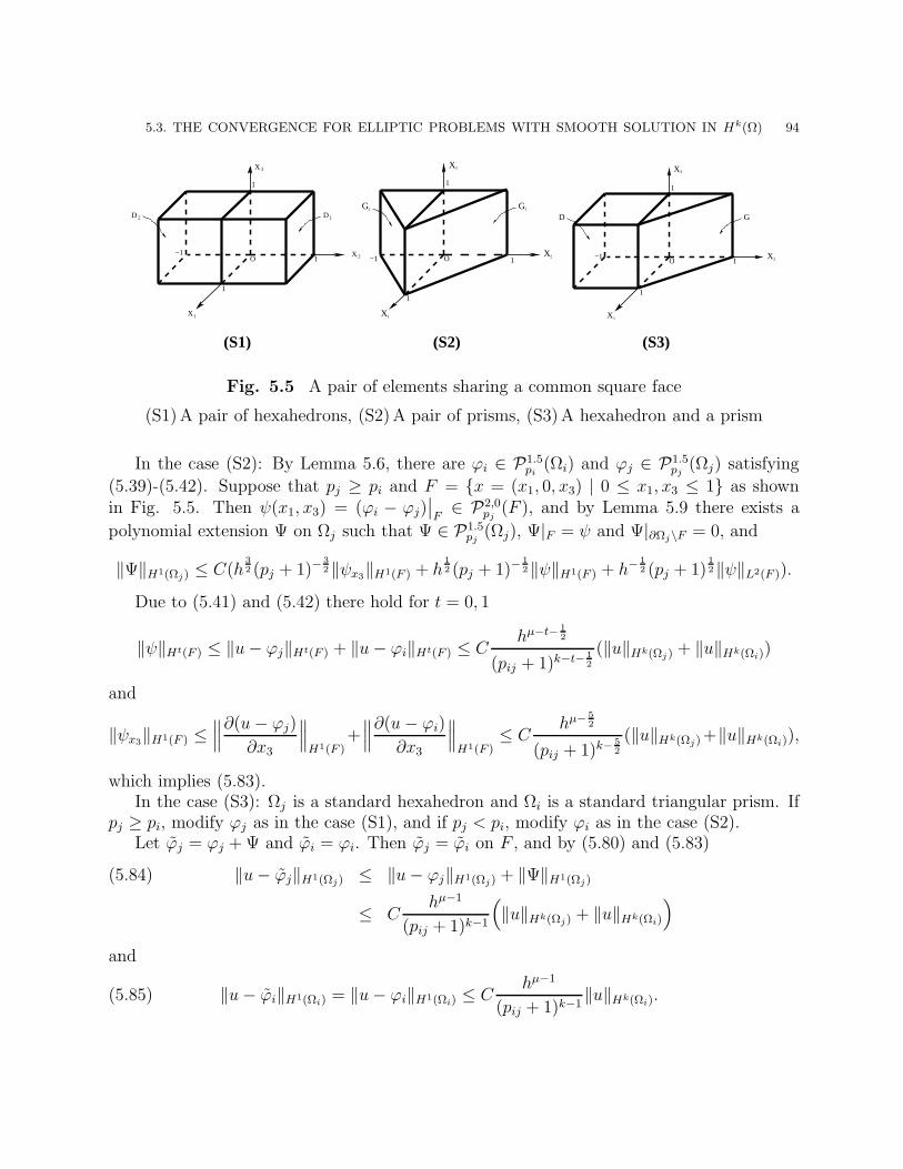
5.3. THE CONVERGENCE FOR ELLIPTIC PROBLEMS WITH SMOOTH SOLUTION IN Hk(Ω) 94
X
X
1
3
1
1
O
G2 G1
−1
1
X2
X
X
1
3
O 1
1
GD
1
−1 X2
X
X 3
O 1
D 2 D1
−1
1
X 2
1
1
(S2) (S3)(S1)
Fig. 5.5 A pair of elements sharing a common square face
(S1)A pair of hexahedrons, (S2)A pair of prisms, (S3)A hexahedron and a prism
In the case (S2): By Lemma 5.6, there are ϕi ∈ P1.5pi
(Ωi) and ϕj ∈ P1.5pj
(Ωj) satisfying
(5.39)-(5.42). Suppose that pj ≥ pi and F = x = (x1, 0, x3) | 0 ≤ x1, x3 ≤ 1 as shownin Fig. 5.5. Then ψ(x1, x3) = (ϕi − ϕj)
∣∣F
∈ P2,0pj
(F ), and by Lemma 5.9 there exists a
polynomial extension Ψ on Ωj such that Ψ ∈ P1.5pj
(Ωj), Ψ|F = ψ and Ψ|∂Ωj\F = 0, and
‖Ψ‖H1(Ωj) ≤ C(h32 (pj + 1)−
32‖ψx3‖H1(F ) + h
12 (pj + 1)−
12‖ψ‖H1(F ) + h−
12 (pj + 1)
12‖ψ‖L2(F )).
Due to (5.41) and (5.42) there hold for t = 0, 1
‖ψ‖Ht(F ) ≤ ‖u− ϕj‖Ht(F ) + ‖u− ϕi‖Ht(F ) ≤ Chµ−t− 1
2
(pij + 1)k−t− 12
(‖u‖Hk(Ωj) + ‖u‖Hk(Ωi))
and
‖ψx3‖H1(F ) ≤∥∥∥∂(u− ϕj)
∂x3
∥∥∥H1(F )
+∥∥∥∂(u− ϕi)
∂x3
∥∥∥H1(F )
≤ Chµ− 5
2
(pij + 1)k− 52
(‖u‖Hk(Ωj)+‖u‖Hk(Ωi)),
which implies (5.83).In the case (S3): Ωj is a standard hexahedron and Ωi is a standard triangular prism. If
pj ≥ pi, modify ϕj as in the case (S1), and if pj < pi, modify ϕi as in the case (S2).Let ϕj = ϕj + Ψ and ϕi = ϕi. Then ϕj = ϕi on F , and by (5.80) and (5.83)
‖u− ϕj‖H1(Ωj) ≤ ‖u− ϕj‖H1(Ωj) + ‖Ψ‖H1(Ωj)(5.84)
≤ Chµ−1
(pij + 1)k−1
(‖u‖Hk(Ωj) + ‖u‖Hk(Ωi)
)
and
‖u− ϕi‖H1(Ωi) = ‖u− ϕi‖H1(Ωi) ≤ Chµ−1
(pij + 1)k−1‖u‖Hk(Ωi).(5.85)

5.3. THE CONVERGENCE FOR ELLIPTIC PROBLEMS WITH SMOOTH SOLUTION IN Hk(Ω) 95
Adjusting ϕj on each face of Ωj by the lifting polynomial Ψ, we achieve the continuityacross interfaces of elements. For the homogeneous Dirichlet boundary condition, we canadjust ϕj in similar way such that ϕj |∂Ωj∩ΓD
= 0. Let ϕ = ϕj in Ωj , 1 ≤ j ≤ J . Then
ϕ ∈ Sp,1D (Ω; ∆h;M), and satisfies (5.79).
We next prove (5.79) for 1 < k < 3 and p ≥ 2. It was shown in, e.g., [2] that Hk(Ω) ∩H1
D(Ω) =(H1
D(Ω), H3(Ω) ∩H1D(Ω)
)θ,2
⊂(H1(Ω), H3(Ω)
)θ,2
∩H1D(Ω) with θ = k−1
2∈ (0, 1)
for 1 < k < 3. Since(H1(Ω), H3(Ω)
)θ,2
⊂(H1(Ω), H3(Ω)
)θ,∞
= Bk(Ω), Hk(Ω)∩H1D(Ω) ⊂
Bk(Ω)∩H1D(Ω). Suppose that v ∈ H1
D(Ω) and w ∈ H3(Ω)∩H1D(Ω) form a decomposition of
u ∈ Bk(Ω) ∩H1D(Ω). Applying (5.79) for k = 3, we have a polynomial ϕ ∈ Sp,1
D (Ω; ∆h;M)with p ≥ 2 such that
‖w − ϕp‖H1(Ω) ≤ Ch2
(p+ 1)2‖w‖H3(Ω).
Therefore, we have for any decomposition v and w of u
‖u− ϕ‖H1(Ω) ≤ ‖v‖H1(Ω) + ‖w − ϕ‖H1(Ω)
≤ C(‖v‖H1(Ω) +
h2
(p+ 1)2‖w‖H3(Ω)
)= C
(‖v‖H1(Ω) + t1‖w‖H3(Ω)
)
with t1 = h2
(p+1)2and C independent of v and w. Due to the definition of the Besov space
Bk(Ω), we have
‖u− ϕ‖H1(Ω) ≤ CK(t1, u) ≤ Ctθ1 supt>0
t−θK(t, u) ≤ Ctθ1‖u‖Bk(Ω) ≤ Chk−1
(p+ 1)k−1‖u‖Hk(Ω),
which is (5.78) for p ≥ 2 and 1 < k < 3.For p = 1 and k ≥ 2, by Theorem 5.4 there exist polynomials φj ∈ Pκ
p (Ωj)(κ =1, or 1.5, or 2 if Ωj is a tetrahedron, or a prism or a hexahedron respectively) in eachelement Ωj such that u = ϕj at each vertex V of Ωj , and
‖u− φj‖Hl(Ωj) ≤ Chµ−1
(pj + 1)k−l‖u‖Hk(Ωj),(5.86)
Let ϕ = φj in Ωj , 1 ≤ j ≤ J . Then ϕ ∈ Sp,1D (Ω; ∆h;M), and satisfies (5.79).
For p = 1 and 1 < k < 2, similarly, it holds that Hk(Ω) ∪ H1D(Ω) =
(H1
D(Ω), H2(Ω) ∩H1
D(Ω))
θ,2⊂
(H1(Ω), H3(Ω)
)θ,2
∩ H1D(Ω) with θ = k − 1 ∈ (0, 1) for 1 < k < 3. Since
(H1(Ω), H2(Ω)
)θ,2
⊂(H1(Ω), H2(Ω)
)θ,∞
= Bk(Ω), Hk(Ω) ∩ H1D(Ω) ⊂ Bk(Ω) ∩ H1
D(Ω).
Suppose that v ∈ H1D(Ω) and w ∈ H2(Ω) ∩ H1
D(Ω) form a decomposition of u ∈ Bk(Ω) ∩H1
D(Ω). Applying (5.79) for k = 2, we have a polynomial ϕ ∈ Sp,1D (Ω; ∆h;M) with p = 1

5.3. THE CONVERGENCE FOR ELLIPTIC PROBLEMS WITH SMOOTH SOLUTION IN Hk(Ω) 96
such that
‖w − ϕp‖H1(Ω) ≤ Ch
(p+ 1)‖w‖H2(Ω).
Arguing as for 1 < k < 3 and p ≥ 2 we can shown that
‖u− ϕ‖H1(Ω) ≤ CK(t1, u) ≤ Ctθ1 supt>0
t−θK(t, u) ≤ Ctθ1‖u‖Bk(Ω) ≤ Chk−1
(p+ 1)k−1‖u‖Hk(Ω),
which is (5.78) for p = 2 and 1 < k < 2.For p = 0 or k = 1, (5.79) is trivial by selecting ϕ = 0. Thus we complete the proof of
the theorem.
5.3.2. Elliptic problems with non-homogeneous Dirichlet condition.
Consider a boundary value problem with non-homogeneous Dirichlet boundary condition
−∆u + u = f in Ω ⊂ R3
u |ΓD= q,
∂u
∂n
∣∣ΓN
= g,
(5.87)
where Ω is Lipschitz domain in R3, and ΓD and ΓN are referred as the Dirichlet boundary
and the Neumann boundary where the Dirichlet and Neumann boundary conditions areimposed.
Lemma 5.11. Let u ∈ Hs(Sh), Sh = (−h, h)2 with s > 1. Then there exists a polynomialϕ ∈ P2
p (Sh) satisfying
‖u− ϕ‖Hl(Sh) ≤ Chµ−l
(p+ 1)s−l‖u‖Hs(Sh), 0 ≤ l ≤ 1(5.88)
ϕ(Vi) = u(Vi), 1 ≤ i ≤ 4(5.89)
ϕ|γi= πγi
u, 1 ≤ i ≤ 4(5.90)
where µ = min (p+ 1, s), Vi and γi are vertices and sides of Sh and πγiis the operator defined
as in Lemma 5.2.
Proof. We first prove the lemma for integers s and l. By Lemma 4.2 of [34] there exists apolynomial φ ∈ P2
p (Sh) such that φ(Vi) = u(Vi), 1 ≤ i ≤ 4, and
‖u− φ‖Hl(Sh) ≤ Chµ−l
(p+ 1)s−l‖u‖Hs(Sh), 0 ≤ l ≤ s, µ = minp+ 1, s.
To construct a desired polynomial ψ ∈ P2p (Sh), let ϕ = φ+ v with v ∈ P2
p (Sh) satisfying
v(Vi) = 0, 1 ≤ i ≤ 4,(5.91)
v|γi = πγiu− φ|γi, 1 ≤ i ≤ 4,(5.92)

5.3. THE CONVERGENCE FOR ELLIPTIC PROBLEMS WITH SMOOTH SOLUTION IN Hk(Ω) 97
‖v‖Hl(Sh) ≤ Chµ−l
ps−l‖u‖Hs(Sh), 0 ≤ l ≤ s.(5.93)
For s > 1, u ∈ Hs− 12 (γi). By Lemma 5.2 πγi
u = u at ending points Vi and Vi+1, and
‖u− πγiu‖Hl(γi) ≤ C
hµ− 12−l
(p+ 1)s− 12−l‖u‖
Hs−12 (γi)
, 0 ≤ l ≤ s− 1
2.
Then gi = πγiu− φ|γi
∈ P0p (γi), and
‖gi‖Ht(γi) ≤ ‖u− πγiu‖Ht(γi) + ‖u− φ‖Ht(γi)(5.94)
≤ C( hµ−t− 1
2
(p+ 1)s−t− 12
‖u‖Hs−1
2 (γi)+ ‖u− φ‖
Ht+12 (S)
)
≤ Chµ−t− 1
2
(p+ 1)s−t− 12
‖u‖Hs(S).
Let v1 = g1(x1)ψ(x2) with ψ(x2) =(h− x2
2h
)p
, then we have
‖ψ‖Ht(I) ≤ Ch12−tpt− 1
2 , t = 0, 1.(5.95)
Then v1|γ1 = g1 and v1 = 0 on γi, 2 ≤ i ≤ 4, and due to (5.95) and (5.94) there holds for0 ≤ l ≤ s
|v1|2Hl(S) ≤ C(‖g1‖2Hl(I)‖ψ‖2
L2(I) + ‖g‖2L2(I)‖ψ‖2
Hl(I))
≤ C( h2(µ−l− 1
2)
(p+ 1)2(s−l− 12)hp−1 +
h2(µ− 12)
(p+ 1)2(s− 12)h2( 1
2−l)p2(l− 1
2))‖u‖2
Hs(S)
≤ h2(µ−l)
(p+ 1)−2(s−l)‖u‖2
Hs(S).
Similarly we can construct vi ∈ P2p (γi), 1 ≤ i ≤ 4 such that vi(Vj) = 0
vi|γi= gi, vi|γj
= 0 for j 6= i, 1 ≤ j ≤ 4
and
‖vi‖Hl(S) ≤ Chµ−l
(p+ 1)s−l‖u‖Hs(S).
Let v =∑4
i=1 vi. Then v satisfies (5.91)-(5.93), and (5.88)-(5.90) follow for integer land s. The results can be generalized to non-integer l and s by the standard argument ofinterpolation spaces.
5.3. THE CONVERGENCE FOR ELLIPTIC PROBLEMS WITH SMOOTH SOLUTION IN Hk(Ω) 98
Lemma 5.12. Let u ∈ Hs(Th) with s > 1, where Th is a triangle (x1, x2)|0 ≤ x2 ≤h− x1, 0 ≤ x1 ≤ h. Then there exists a polynomial ϕ(x) ∈ P1
p (Th) such that
‖u− ϕ‖Hl(Th) ≤ Chµ−l
(p+ 1)s−l‖u‖Hs(Th), l = 0, 1,(5.96)
ϕ(Vi) = u(Vi), 1 ≤ i ≤ 3,(5.97)
ϕ|γi = πγiu, 1 ≤ i ≤ 3(5.98)
where µ = minp+1, s, Vi and γi are vertices and sides of Th and πγiis the operator defined
as in Lemma 5.2.
Proof. We may prove the lemma for integer s and l because the desired results for non-integer l and s follow easily by the standard argument of interpolation space.
By Lemma 4.2 of [34] there exists a polynomial φ ∈ P1p (Th) such that φ(Vi) = u(Vi),
1 ≤ i ≤ 3 and
‖u− φ‖Hl(Th) ≤ Chµ−l
(p+ 1)s−l‖u‖Hs(Th), 0 ≤ l ≤ s, µ = minp+ 1, s.(5.99)
By Lemma 5.2, πγiu = u at the ending points Vi and Vi+1, and
‖u− πγiu‖Ht(γi) ≤ C
hµ− 12−t
(p+ 1)s− 12−t‖u‖
Hs−12 (γi)
(5.100)
≤ Chµ− 1
2−t
(p+ 1)s− 12−t‖u‖Hs(Th)
Then gi = (πγiu− φ|γi
) ∈ P0p (γi), and (5.99)-(5.100) lead to the following estimates which is
an analogue to (5.94)
‖gi‖Ht(γi) ≤ Chµ− 1
2−t
(p+ 1)s− 12−t‖u‖Hs(Th), 0 ≤ t ≤ s− 1
2.(5.101)
By Lemma 5.3, there exists an extension vi ∈ P1p (Th) such that for t = 0, 1
vi(Vj) = 0, 1 ≤ j ≤ 3,(5.102)
vi|γi= gi, vi|γj
= 0, j 6= i, 1 ≤ j ≤ 3,(5.103)
‖vi‖Hl(Th) ≤ C(h32−l(p+ 1)l− 3
2‖gi‖H1(γi) + h12−l(p+ 1)l− 1
2‖gi‖L2(γi))(5.104)
≤ Chµ−l
(p+ 1)s−l‖u‖Hs(Th).
Let ϕ = φ+∑3
i=1 vi. Then ϕ ∈ P1p (Th) and satisfies (5.96)-(5.98).
The partition ∆h on Ω induces a partition ∆γi= Γi,j, j ∈ Ji on Γi, i ∈ D where Ji is a
subset of J = 1, 2, · · · , J, and a partition ∆ΓD= ∆Γi
, i ∈ D on ΓD. Γi,j’s are (curved)

5.3. THE CONVERGENCE FOR ELLIPTIC PROBLEMS WITH SMOOTH SOLUTION IN Hk(Ω) 99
triangles and quadrilaterals. By Vi,j,l and γi,j,l we denote vertices and sides of Γi,j, then∆Γi
and ∆ΓDare the restrictions of the partition ∆h of Ω on Γi and ΓD. For i ∈ D, Let
SP,1(Γi,∆Γi,MΓi,j
) be the restriction on ∆Γiof polynomials in SP,1(Ω; ∆h;M), ie.
SP,1(Γi; ∆i;MΓi) = ϕ | ϕ|Γi,j
Mi,j ∈ P 1pj
(Th) or P 2pj
(Sh) ∩H1(Γi)
where MΓi= Mi,j, 1 ≤ j ≤ J(i), i ∈ D and Mi,j is the restriction of the map Mj on Γi,j
which maps a standard triangle or a square with size h onto Γi,j. By SP,1(ΓD; ∆ΓD;MΓD
)we denote the union of SP,1(Γi; ∆Γi
;MΓi), i ∈ D.
Lemma 5.13. Let qi be the restriction of g on Γi, i ∈ D and let qi ∈ Hs(Γi), s > 1. Thenthere exist a polynomial qi,p ∈ SP,1(Γi; ∆Γi
;MΓi) such that for integer l, 0 ≤ l ≤ s
‖qi − qi,p‖Hl(ΓD) ≤ Chµ−l
(pi + 1)s−l‖qi‖Hs(Γi)(5.105)
with µ = minp+ 1, s, pi = minj∈Ji
pj.
Proof. By Lemma 5.11 and Lemma 5.12, there exists a polynomial ψi,j ∈ Pκpj
(Γi,j), κ =1 or 2, respectively, such that
‖qi − ψi,j‖Hl(Γi,j) ≤ Chµ−l
(pj + 1)s−l‖qi‖Hs(Γi,j ),
qi(Vi,j,l) = ψi,j(Vi,j,l), 1 ≤ l ≤ 3 or 4,
ψij |γi,j,l= πγi,j,l
qi, 1 ≤ l ≤ 3 or 4.
Let qi,p = ψi,j on Γi,j, j ∈ Ji. Then qi,p ∈ SP,1(Γi; ∆Γi;MΓi
) and
‖qi − qi,p‖2Hl(Γi)
≤∑
j∈Ji
‖qi − ψi,j‖2Hl(Γi,j)
≤ C∑
j∈Ji
h2(µ−l)
(pj + 1)2(s−l)‖qi‖2
Hs(Γi,j)
≤ Ch2(µ−l)
(pi + 1)2(s−l)‖qi‖2
Hs(Γi).
Corollary 5.14. Let wi,p ∈ SP,1(Γi; ∆i;MΓi) be the finite element solution of the boundary
value problem∫
Γi
(∇w∇v + wv)dS =
∫
Γi
(∇qi∇v + qiv)dS, ∀v ∈ SP,1(Γi; ∆i;MΓi) ∩H1
0 (Γi),
w |∂Γi= πγi,j,l
q, γi,j,l = ∂Γi,j ∩ ∂Γi, j ∈ Ji.
(5.106)
Then
‖qi − wi,p‖Hl(Γi) ≤ Chµ−l
(pi + 1)s−l‖qi‖Hs(Γi),

5.3. THE CONVERGENCE FOR ELLIPTIC PROBLEMS WITH SMOOTH SOLUTION IN Hk(Ω) 100
where µ = minpi, s.
Remark 5.1. Lemma 5.13 indicates the existence of the polynomial qi,p ∈ SP,1(Γi; ∆Γi;MΓi
)satisfying (5.105). Notice that such a polynomial is not unique. Corollary 5.14 gives apractical way to construct the polynomial qi,p by compute a finite element solution wi,p.
Define qp on ΓD such that qp = qi,p on Γi, i ∈ D. Then qp ∈ C0(ΓD) and qp ∈SP,1(ΓD; ∆ΓD
;MΓD). Due to (5.105) there holds for t = 0, 1
‖q − qp‖Ht(ΓD) ≤∑
i∈D‖qi − qi,p‖Ht(Γi) ≤ C
∑
i∈D
hµ− 12−t
(pi + 1)k− 12−t‖qi‖Hk−1
2 (Γi)(5.107)
≤ Chµ− 1
2−t
(p+ 1)k− 12−t
∑
i∈D‖qi‖Hk− 1
2 (Γi),
where p = minj∈J
pj. By the standard argument of interpolation spaces (5.107) can be proved
for 0 < t < 1.Now we formulate the finite element solution for boundary value problem (5.87) with
non-homogeneous Dirichlet boundary condition: Find up such that
∫
Ω
(∇up∇v + up v)dx =
∫
Ω
fvdx+
∫
ΓN
gvdS, ∀v ∈ SP,1D (Ω; ∆h;M)
up ∈ SP,1(Ω; ∆h;M), up |ΓD= qp.
(5.108)
Obviously up is the finite element approximation to the solution u of the following boundaryvalue problem
∫
Ω
(∇u∇v + u v)dx =
∫
Ω
fvdx+
∫
ΓN
gvdS, ∀v ∈ H1D(Ω),
u ∈ H1(Ω), u |ΓD= qp.
(5.109)
Lemma 5.15. Let u and up be the solution of the problem (5.109) and the finite elementsolution satisfying (5.108). Then
B(u− up, v) =
∫(∇(u− up)∇v + (u− up)v)dx = 0, ∀v ∈ SP,1(Ω; ∆h;M)(5.110)
and
‖u− up‖H1(Ω) = infw∈SP,1(Ω;∆h;M)w|ΓD
=qp
‖u− w‖H1(Ω).(5.111)

5.3. THE CONVERGENCE FOR ELLIPTIC PROBLEMS WITH SMOOTH SOLUTION IN Hk(Ω) 101
Proof. (5.110) follows from (5.108) and (5.109) directly. For any w ∈ SP,1(Ω; ∆h;M) withw|ΓD
= qp we have by (5.107)
B(u− w, u− w) = B(u− up, u− up) +B(up − w, up − w) + 2B(u− up, up − w)
= B(u− up, u− up) +B(up − w, up − w)
≥ B(u− up, u− up),
which implies (5.111).
Theorem 5.16. Let u ∈ Hk(Ω) be the solution of the problem of (5.87) and q ∈ C0(ΓD),qi = q|Γi
∈ Hk−1(Γi), i ∈ D, and let up ∈ SP,1(Ω; ∆h;M) with p ≥ 1 be the finite elementsolution of (5.108) with up|ΓD
= qp ∈ SP,1(ΓD; ∆ΓD;MΓD
) satisfying (5.107). Then
‖u− up‖H1(Ω) ≤ Chµ−1
(p+ 1)k−1‖u‖Hk(Ω), µ = minp+ 1, k.(5.112)
Proof. Note that
‖u− up‖H1(Ω) ≤ ‖u− u‖H1(Ω) + ‖u− up‖H1(Ω).(5.113)
Since u− u satisfies
∆(u− u) = 0
∂
∂n(u− u)|ΓN
= 0, (u− u)|ΓD= q − qp.
By the continuous dependence of solution on boundary condition and (5.107), we have
‖u− u‖H1(Ω) ≤ C‖q − qp‖H12 (ΓD)
≤ Chµ−1
(p+ 1)k−1
∑
i∈D‖qi‖Hk− 1
2 (Γi).(5.114)
Due to (5.111) it is sufficient to construct a polynomial ϕ ∈ SP,1(Ω; ∆h;M) such thatϕ|ΓD
= qp and
‖u− ϕ‖H1(Ω) ≤ Chµ−1
(p+ 1)k−1‖u‖Hk(Ω).(5.115)
By the argument in proof of Theorem 5.10, there is a polynomial ϕ ∈ SP,1(Ω; ∆h;M) suchthat
‖u− ϕ‖Ht(Ω) ≤ Chµ−t
(p+ 1)k−t‖u‖Hk(Ω), t = 0, 1, 2,(5.116)
where µ = p + 1, k, p = minj∈J
pj , and u = ϕ at vertices of Ωj ’s and u|γ = πγu on each side
of elements. It remains to adjust ϕ on ΓD. Suppose that Γi,j = ∂Ωj
⋂Γi for some i ∈ D is
a face of Ωj . Then φ = (qi,p − ϕ) |Γi,j∈ Pκ,0
pj(Γi,j) with κ = 1 or 2. Hence there exists an
extension Φ ∈ Pκpj
(Ωj) such that Φ|Γi,j= φ and Φ|∂Ωj\Γi,j
= 0, and by Lemma 5.8
‖Φ‖H1(Ωj) ≤ C‖φ‖H
1200(Γi,j )

5.4. THE CONVERGENCE FOR PROBLEMS ON POLYHEDRAL DOMAINS 102
if Ωj is a tetrahedron or hexahedron with κ = 1 or 2 or Γi,j is a triangular face of prism withκ = 1.5, and
‖Φ‖H1(Ωj) ≤ C( ∑
0≤t≤1
ht− 12
(pj + 1)t− 12
‖φ‖Ht(Γi,j) + h32 (pj + 1)−
32
∥∥∥ ∂φ∂x3
∥∥∥H1(Γi,j)
)(5.117)
if Ωj is a triangular prism with κ = 1.5 and all Γi,j is its square face.If Ωj is tetrahedron or hexahedron or Γi,j is a triangular face of a prism it holds that by
Lemma 5.13 and Lemma 5.6 for t = 0, 1
‖qi,p − ϕ‖Ht(Γi,j) ≤ ‖qi,p − qi‖Ht(Γi,j ) + ‖u− ϕ‖Ht(Γi,j)
≤ Chµ− 1
2−t
(pj + 1)k− 12−t
(‖q‖Hk−1
2 (Γi,j )+ ‖u‖Hk(Ωj)),
by the standard argument of interpolation space for H1200(Γij) = (L2(Γi,j, H
10 (Γi,j)) 1
2there
holds
‖Φ‖H1(Ωj) ≤ ‖qi,p − ϕ‖H
1200(Γi,j)
≤ Chµ−1
(pj + 1)k−1(‖qi‖Hk− 1
2 (Γi,j)+ ‖u‖Hk(Ωj))
≤ Chµ−1
(pj + 1)k−1‖u‖Hk(Ωj).
If Ωj is a prism and Γi,j is a square face, we have by Lemma 5.6 and Lemma 5.13 for t = 0, 1
‖Φ‖H1(Ωj) ≤ C1∑
t=0
hµ− 12
(pj + 1)t− 12
(‖u− ϕ‖Ht(Γi,j) + ‖qi − qi,p‖Ht(Γi,j))(5.118)
+ h32 (pj + 1)−
32
∥∥∥∂u − ϕ
∂x3
∥∥∥H1(Γi,j )
≤ Chµ−1
(pj + 1)k−1‖u‖Hk(Ωj).
Let ϕj = ϕj + Φ on Ωj . Then ϕj|Γi,j= qi,p|Γi,j, and by (5.116) and (5.117)
‖u− ϕj‖H1(Ωj) ≤ Chµ−1
(pj + 1)k−1‖u‖Hk(Ωj).
The treatment Γi,j can be carried out on each face of Ωj which is on ΓD. Let ϕ = ϕj +Φj
on Ωj if ∂Ωj ∩ ΓD 6= ∅ and ϕ = ϕj on Ωj if ∂Ωj ∩ ΓD = ∅. Then ϕ ∈ SP,0(Ω; ∆h;M) andϕ|ΓD
= qp, and satisfies (5.115). A combination of (5.113)-(5.115) leads to (5.112).
5.4. The convergence for problems on polyhedral domains
In this section we will investigate the optimal convergence of the h-p version of the finiteelement method for elliptic problems on polyhedral domains by combining the previousresults on smooth and singular functions in the framework of Jacobi-weighted Besov andSobolev spaces.

5.4. THE CONVERGENCE FOR PROBLEMS ON POLYHEDRAL DOMAINS 103
Let Ω be a polyhedral domain in R3, shown in Fig. 5.1, and let Γi, i ∈ I = 1, 2, 3, . . . , I,
be the faces(open), Λij be the edges, which are the intersections of Γi and Γj, and Am, m ∈M = 1, 2, . . . ,M, be the vertices of Ω. By Jm we denote a subset j ∈ J |Am ∈ Γj of Jfor m ∈ M. Let L = ij|i, j ∈ J , Γi ∩ Γj = Λij, and let Lm denote a subset of L such thatLm = ij ∈ L|Am ∈ Γi ∩ Γj = Λij. We denote by ωij the interior angle between Γi and Γj
for ij ∈ L. Let Γ0 = ∪i∈DΓi and Γ1 = ∪i∈NΓi, where D is a subset of J and N = J \D.For m ∈ M,Dm = D ∩ Jm and Nm = N ∩ Jm.
In order to study effectively the regularity of the solutions of elliptic problems on a polyhe-dral domain, we shall decompose the domain into various neighborhoods of low dimensionalmanifolds.
νδ,σ(Α1,Λ1,2)
Λ Λ
Λ12Λ12
X
X
1
3
A1
Γ
Γ σ
δ
ω12
1
2
2
XX3
A
X1
X
XA
2
3
2
δ/2
δ/2ω Γ
Λ
4
12
2
Γ1
12
Λ23
13
A1
Λ12
δ
2Γ
X3
Λ23
νδ,σ Α1, Λ )(
A1
Γ3
Λ12
Γ1
δ
2Γ
13
νδ,σ(Α1,Λ )23
µε,δ
νδ,σ(Α1,Λ1,2)
( )
O (Α1)δ
1Oδ Α )(∼13
(c)
(d)
(a)
(b)
Fig. 5.6 Neighborhoods of edges and vertices:
(a) the neighbourhood Uεij ,δij(Λij); (b) the neighborhood Oδm(Am);
(c) the neighborhood Vδℓ,σij(Aℓ,Λij); (d) the inner-neighborhood Oδm(Am).
We define a neighborhood Uεij ,δij(Λij) of the edge Λij, shown in Fig. 5.6(a), and assume
that Λij = x = (x1, x2, x3)|x1 = x2 = 0, a ≤ x ≤ b, as follows:
Uεij ,δij(Λij) = x ∈ Ω|0 ≤ r = dist(x,Λij) < εij, a+ δij < x3 < b− δij.
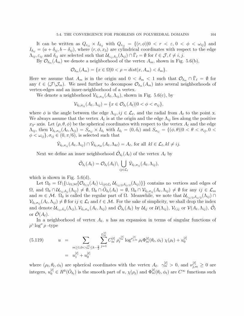
5.4. THE CONVERGENCE FOR PROBLEMS ON POLYHEDRAL DOMAINS 104
It can be written as Qεij× Iδij
with Qεij= (r, φ)|0 < r < ε, 0 < φ < ωij and
Iδij= (a + δij , b − δij), where (r, φ, x3) are cylindrical coordinates with respect to the edge
Λij, εij and δij are selected such that Uεij ,δij(Λij) ∩ Γℓ = ∅ for ℓ ∈ J , ℓ 6= i, j.
By Oδm(Am) we denote a neighborhood of the vertex Am, shown in Fig. 5.6(b),
Oδm(Am) = x ∈ Ω|0 < ρ = dist(x,Am) < δm.Here we assume that Am is in the origin and 0 < δm < 1 such that Oδm ∩ Γℓ = ∅ forany ℓ ∈ (J \Jm). We need further to decompose Oδm(Am) into several neighborhoods ofvertex-edges and an inner-neighborhood of a vertex.
We denote a neighborhood Vδℓ,σij(Aℓ,Λij), shown in Fig. 5.6(c), by
Vδℓ,σij(Aℓ,Λij) = x ∈ Oδℓ
(Aℓ)|0 < φ < σij,where φ is the angle between the edge Λij, ij ∈ Lℓ, and the radial from Aℓ to the point x.We always assume that the vertex Aℓ is at the origin and the edge Λij lies along the positivex3- axis. Let (ρ, θ, φ) be the spherical coordinates with respect to the vertex Aℓ and the edgeΛij, then Vδℓ,σij
(Aℓ,Λij) = Sσij× Iδℓ
with Iδℓ= (0, δℓ) and Sσij
= (φ, θ)|0 < θ < σij , 0 <φ < ωij, σij ∈ (0, π/6), is selected such that
Vδℓ,σij(Aℓ,Λij) ∩ Vδℓ,σkl
(Aℓ,Λkl) = Aℓ, for all kl ∈ Lℓ, kl 6= ij.
Next we define an inner neighborhood Oδℓ(Aℓ) of the vertex Aℓ by
Oδℓ(Aℓ) = Oδℓ
(Aℓ)\⋃
ij∈Lℓ
Vδℓ,σij(Aℓ,Λij),
which is shown in Fig. 5.6(d).Let Ω0 = Ω\∪ℓ∈MOδℓ/2
(Aℓ) ∪ij∈LℓUεij/2,δij/2
(Λij) contains no vertices and edges of
Ω, and Ω0 ∩ Uεij ,δij(Λij) 6= ∅, Ω0 ∩ Oδℓ
(Aℓ) = ∅, Ω0 ∩ Vδℓ,σij(Aℓ,Λij) 6= ∅ for any ij ∈ Lm
and m ∈ M. Ω0 is called the regular part of Ω. Meanwhile, we note that Uεij/2,δij/2(Λij) ∩
Vδℓ,σij(Aℓ,Λij) 6= ∅ for ij ∈ Lℓ and ℓ ∈ M. For the sake of simplicity, we shall drop the index
and denote Uεij ,δij(Λij),Vδℓ,σij
(Aℓ,Λij) and Oδℓ(Aℓ) by Uij or U(Λij), Vℓ,ij or V(Aℓ,Λij), Oℓ
or O(Aℓ).In a neighborhood of vertex Aℓ, u has an expansion in terms of singular functions of
ργ logν ρ -type
u =∑
m≥1,0<γ[ℓ]m ≤k− 3
2
L[ℓ]m∑
j=1
C [ℓ]m ργ
[ℓ]m
ℓ logν[ℓ]j,m ρℓΦ
[ℓ]m(θℓ, φℓ) χ(ρℓ) + u
[ℓ]0(5.119)
= u[ℓ]1 + u
[ℓ]0
where (ρℓ, θℓ, φℓ) are spherical coordinates with the vertex Aℓ. γ[ℓ]m > 0, and ν
[ℓ]j,m ≥ 0 are
integers, u[ℓ]0 ∈ Hk(Oδℓ
) is the smooth part of u, χ(ρℓ) and Φ[ℓ]m(θℓ, φℓ) are C∞ functions such

5.4. THE CONVERGENCE FOR PROBLEMS ON POLYHEDRAL DOMAINS 105
that χ(ρℓ) = 1 for 0 < ρℓ < δℓ/2 and χ(ρℓ) = 0 for ρℓ > δℓ. We assume that γ[ℓ]m < γ
[ℓ]m+1 and
ν[ℓ]j,m > ν
[ℓ]j+1,m.
In a neighborhood of edge Λij, ij ∈ L, u has an expansion in terms of singular functionsof rσ logµ r -type
u =∑
m≥1,0<σ[ij]m ≤k− 3
2
C [ij]m rσ
[ij]m
ij
L[ij]m∑
l=1
logµ[ij]l,m rij χ(rij)Φ
[ij]m (φij)Ψ
[ij](x3) + u[ij]0(5.120)
= u[ij]1 + u
[ij]0
where (rij , φij, x3) are cylindrical coordinates with the edge Λij. σ[ij]m > 0, and µ
[ij]l,m ≥ 0 are
integers, u[ij]0 ∈ Hk(Uεij ,δij
(Λij)) is the smooth part of u, χ(rij), Φ[ij]m (φij) and Ψ[ij](x3) are
C∞ functions such that χ(rij) = 1 for 0 < rij < εij/2 and χ(rij) = 0 for rij ≥ εij. We
assume that σ[ij]m < σ
[ij]m+1 and µ
[ij]l,m > µ
[ij]l+1,m+1.
In a neighborhood of vertex-edge Aℓ-Λij, ℓ ∈ M, ij ∈ Lℓ, u has an expansion in terms ofsingular functions of ργ logν ρ sinσ θ logµ sin θ -type
u =∑
0<γ[ℓ]m ≤k− 3
2
C[ℓ,ij]m,j,s,tρ
γ[ℓ]m
m
L[ij]ℓ∑
j=1
logν[ℓ]j,m ρm
∑
0<σ[ij]s ≤k−1
(sin θij)σ
[ij]s
Ts∑
t=1
logµ[ij]t,s sin θij χ(ρℓ)Φ
[ℓ,ij]m (θij)Ψ
[ℓ,ij]m (φij) + u
[ℓ,ij]0(5.121)
= u[ℓ,ij]1 + u
[ℓ,ij]0 .
where (ρm, θij , φij) are spherical coordinates with the vertex-edge Aℓ-Λij. γ[ℓ]m > 0, ν
[ℓ]j,m ≥ 0,
σ[ij]s > 0 and µ
[ij]t,s are integers, u
[ℓ,ij]0 ∈ Hk(Vδℓ,σij
(Aℓ,Λij)) is the smooth part of u, χ(ρℓ),
Φ[ℓ,ij]m (θij) and Ψ
[ℓ,ij]m (φij) are C∞ functions such that χ(ρℓ) = 1 for 0 < ρℓ < δℓ/2 and
χ(ρℓ) = 0 for ρℓ > δℓ. We assume that γ[ℓ]m < γ
[ℓ]m+1, ν
[ℓ]j,m > ν
[ℓ]j+1,m, σ
[ij]s < σ
[ij]s+1 and
µ[ij]t,s > µ
[ij]t+1,s+1.
Let
(5.122) γ = minℓ∈M
γ[ℓ]1 , νγ = max
ℓ∈M,γ[ℓ]1 =γ
ν[ℓ]1,1, σ = min
ij∈Lσ
[ij]1 , µσ = max
ij∈L,σ[ij]1 =σ
µ[ij]1,1 .
We shall analyze the convergence of the h-p version of the finite element method withquasi-uniform meshes for problems on polyhedral domains.
Lemma 5.17. Let Ωj is a hexahedron or a triangular prism or a tetrahedron elementcontaining a vertex Aℓ of a polyhedron Ω with size hj, and the function u has the ex-
pansion (5.119) with u[ℓ]0 ∈ Hk(Oδℓ
) with k ≥ 2 + 2γ. Then there exists a polynomial

5.4. THE CONVERGENCE FOR PROBLEMS ON POLYHEDRAL DOMAINS 106
(c)(b)(a)
3
X 2
O
ρ0
h−
X
−h
h
R0Sκ 0
hX
X
1
3
X 2
O
0
ρ0
h−h
−h
h
Sκ 0R 0
R
X 1
3
X 2
O
ρ0
h−h
−h
h
S κ 0
X 1
X
Fig. 5.7 3d elements contained in Rhρ0,κ0+ε ⊂ Rh
0 .
(a) A tetrahedron contained in Rhρ0,κ0+ε;
(b) A parallel prism contained in Rhρ0,κ0+ε; (c) A parallelepiped contained in Rh
ρ0,κ0+ε.
ϕj ∈ Pκpj
(Ωj), pj ≥ 1/2 + γ, 1 ≤ κ ≤ 2 such that ϕj = u at the vertices of Ωj and vanisheson ∂Ω ∩ ΓD and and ϕj = 0 on ∂Ωj ∩ ΓD, and
(5.123) ‖u− ϕj‖H1(Ωj) ≤ Ch
12+γ
j
(pj + 1)2γ+1Fνγ (pj , hj)
with the constant C depending on u, γ and νγ, but not on pj and hj, where γ and νγ aregiven in (5.122) and Fνγ (pj , hj) is given as in (3.31).
Proof. We may assume that ℓ = 1. Then the expansion (5.119) holds in Ωj . By Theorem 5.4
and Theorem 5.10, there exists a polynomial ψ0 ∈ Pκpj
(Ωj), 1 ≤ κ ≤ 2 such that ψ0 = u[1]0 at
the vertices of Ωj and vanishes on ∂Ωj ∩ ΓD, and
‖u[1]0 − ψ0‖H1(Ωj) ≤ C
hµj−1j
(pj + 1)k−1
with µj = minpj + 1, k ≥ 32
+ γ. For a sharp approximation to u[1]1 , we map Ωj into
Rh0 = Rh
ρ0,κ0⊂ Qh by an affine mapping Fj such that A1 Mj = (−h,−h,−h) and that
Ωj Mj is contained in Rh0 , as shown in Fig. 5.7. Without losing generality we may assume
that A1 = (−h,−h,−h) and Ωj is a tetrahedron, or a parallelepiped, or a parallel prism whichis contained in Rh
ρ0,κ0+ε ⊂ Rh0 . We extend the function Φ(θ, φ) analytically on (0, π/2; 0, π/2)
such that [θ0, π/2− θ0;φ0, π/2− φ0] is its support. Then u[1]1 ∈ B
2+2γ[1]1
ν[1]∗1,1
(Qh) by Theorem 3.7

5.4. THE CONVERGENCE FOR PROBLEMS ON POLYHEDRAL DOMAINS 107
with
ν[1]∗1,1 =
ν[1]1,1 if γ
[1]1 is not an integer or ν
[1]1,1 = 0,
ν[1]1,1 − 1 if γ
[1]1 is an integer and ν
[1]1,1 ≥ 1,
and there exists polynomials ψ[1]1 ∈ Pκ
pj(Ωj), 1 ≤ κ ≤ 2 due to Theorem 3.8 such that ψ
[1]1 = 0
on ∂Ωm ∩ ΓD and
‖u[1]1 − ψ
[1]1 ‖H1(Ωj) ≤ C
h12+γ
[1]1
j
(pj + 1)2γ[1]1 +1
Fν[1]1,1
(pj, hj) ≤ Ch
12+γ
j
(pj + 1)2γ+1Fνγ (pj, hj).
We now adjust ψ[1]1 to ψ
[1]1 such that ψ
[1]1 satisfies (5.124) and u
[ℓ]1 = ψ
[1]1 at the vertices of
Ωj .We will adjust the polynomial for a hexahedron Ωj since the adjustment on tetrahedron
and prism elements is similar to what follows. To this end, we may assume that Ωj stan-
dard shaped hexahedron (−h/2, h/2)3. Let ψ[1]1 = ψ
[1]1 + χ(x) with χ(x) =
∑1≤l≤8(u
[1]1 −
ψ[1]1 )(Vl)χl(x) where Vl, 1 ≤ l ≤ 8 are the vertices of Ωj and χl(x) are defined in (5.21).
Obviously, ψ[1]1 ∈ P2
pj(Ωj) and u
[1]1 (Vl) = ψ
[1]1 (Vl), 1 ≤ l ≤ 8. By (5.20) and (3.30), we
have
‖χl(x)‖H1(Ωj) ≤ Ch12j (pj + 1)−
12
∑
1≤l≤8
|(u[ℓ]1 − ψ)(Vl)| ≤ C
h12+γ
j
(pj + 1)2γ+1Fνγ (pj , hj),
which implies
‖u[ℓ]1 − ψ
[1]1 ‖H1(Ωj) ≤ ‖u[ℓ]
1 − ψ[1]1 ‖H1(Ωj) + ‖χl(x)‖H1(Ωj)(5.124)
≤ Ch
12+γ
j
(pj + 1)2γ+1Fνγ (pj, hj).
Let ϕj = ψ[1]1 +ψ
[1]0 . Then u
[ℓ]1 = ϕj at the vertices of Ωj and vanishes on ∂Ωm ∩ ΓD, and
‖u− ϕj‖H1(Ωj) ≤ C( h
12+γ
j
(pj + 1)2γ+1Fνγ (pj, hj) +
hµj−1j
(pj + 1)k−1
)≤ C
h12+γ
j
(pj + 1)2γ+1Fνγ (pj , hj).
Lemma 5.18. Let Ωm is a hexahedron or a triangular prism or a tetrahedron element ofsize hj with a side γh on a portion of an edge Λij not including its two ending points and the
function u has the expansion (5.120) with u[ij]0 ∈ Hk(Uεij ,δij
), k ≥ 1 + 2σ. Then there existsa polynomial ϕm ∈ Pκ
pj(Ωj), pj ≥ 1/2 + σ, 1 ≤ κ ≤ 2 such that ϕm = u at the vertices of Ωm
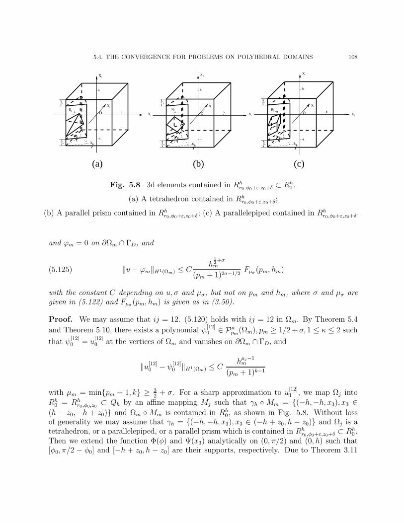
5.4. THE CONVERGENCE FOR PROBLEMS ON POLYHEDRAL DOMAINS 108
(c)(a) (b)
3
X2
O
Z
X
Z 0
φ0
−
0
h
h
φ
h
−h
R0
0φ0 −h
R
X 1 X 1
0
X3
X2
Z0
Z0
φ0
− hh
h
X1
X 3
X 2
O
Z0
Z 0
O
0
− hh
h
φ0 −h
R0
φ
Fig. 5.8 3d elements contained in Rhr0,φ0+ε,z0+δ ⊂ Rh
0 .
(a) A tetrahedron contained in Rhr0,φ0+ε,z0+δ;
(b) A parallel prism contained in Rhr0,φ0+ε,z0+δ; (c) A parallelepiped contained in Rh
r0,φ0+ε,z0+δ.
and ϕm = 0 on ∂Ωm ∩ ΓD, and
(5.125) ‖u− ϕm‖H1(Ωm) ≤ Ch
12+σ
m
(pm + 1)2σ−1/2Fµσ(pm, hm)
with the constant C depending on u, σ and µσ, but not on pm and hm, where σ and µσ aregiven in (5.122) and Fµσ(pm, hm) is given as in (3.50).
Proof. We may assume that ij = 12. (5.120) holds with ij = 12 in Ωm. By Theorem 5.4
and Theorem 5.10, there exists a polynomial ψ[12]0 ∈ Pκ
pm(Ωm), pm ≥ 1/2 + σ, 1 ≤ κ ≤ 2 such
that ψ[12]0 = u
[12]0 at the vertices of Ωm and vanishes on ∂Ωm ∩ ΓD, and
‖u[12]0 − ψ
[12]0 ‖H1(Ωm) ≤ C
hµj−1m
(pm + 1)k−1
with µm = minpm + 1, k ≥ 32
+ σ. For a sharp approximation to u[12]1 , we map Ωj into
Rh0 = Rh
r0,φ0,z0⊂ Qh by an affine mapping Mj such that γh Mm = (−h,−h, x3), x3 ∈
(h − z0,−h + z0) and Ωm Mm is contained in Rh0 , as shown in Fig. 5.8. Without loss
of generality we may assume that γh = (−h,−h, x3), x3 ∈ (−h + z0, h − z0) and Ωj is atetrahedron, or a parallelepiped, or a parallel prism which is contained in Rh
r0,φ0+ε,z0+δ ⊂ Rh0 .
Then we extend the function Φ(φ) and Ψ(x3) analytically on (0, π/2) and (0, h) such that[φ0, π/2 − φ0] and [−h + z0, h − z0] are their supports, respectively. Due to Theorem 3.11

5.4. THE CONVERGENCE FOR PROBLEMS ON POLYHEDRAL DOMAINS 109
and Theorem 3.12, u[ij]1 ∈ B
1+2σ[1]1
µ[1]∗1,1
(Qh) with
µ[1]∗1,1 =
µ[1]1,1 if σ
[1]1 is not an integer or µ
[1]1,1 = 0,
µ[1]1,1 − 1 if σ
[1]1 is an integer and µ
[1]1,1 ≥ 1,
and there exists a polynomial ψ[ij]1 ∈ Pκ
pj(Ωj), pj ≥ 1/2 + σ, 1 ≤ κ ≤ 2 such that ψ
[12]1 = 0 on
∂Ωm ∩ ΓD and
(5.126) ‖u[12]1 − ψ
[12]1 ‖H1(Ωm) ≤ C
h12+σ
[12]1
m
(pm + 1)2σ[12]1
Fµ
[1]1,1
(pm, hm) ≤ Ch
12+σ
m
(pm + 1)2σFµσ(pm, hm).
We next adjust ψ[12]1 to ψ
[12]1 such that u
[ℓ]1 = ψ
[1]1 at the vertices of Ωj and ψ
[1]1 and satisfies
(5.127) ‖u[12]1 − ψ
[12]1 ‖H1(Ωm) ≤ C
h12+σ
m
(pm + 1)2σFµσ(pm, hm).
We will adjust the polynomial for a prism Ωj since the adjustment on tetrahedron andhexahedron elements is similar to what follows. To this end, we may assume that Ωj standard
shaped prism x = (x1, x2, x3) : x1+x2 ≤ 0, xi ∈ (−h/2, h/2), i = 1, 2, 3. Let ψ[1]1 = ψ
[1]1 +χ(x)
with χ(x) =∑
1≤l≤6(u[ℓ]1 − φ)(Vl)χl(x) where Vl, 1 ≤ l ≤ 6 are the vertices of Ωm and χl(x)
are defined in (5.21) for pm ≥ 2 and in (5.24) for pm = 1.
Obviously, ψ[12]1 ∈ P2
pm(Ωm), and u
[12]1 (Vl) = ψ
[12]1 (Vl), 1 ≤ l ≤ 6. By (5.20) and (3.49), we
have
‖χl(x)‖H1(Ωj) ≤ Ch12m(pm + 1)−
12
∑
1≤l≤6
|(u[12]1 − ψ
[12]1 )(Vl)| ≤ C
h12+σ
m
(pm + 1)2σ+1/2Fµσ(pm, hm),
which together with (5.126) implies (5.127).
Let ϕm = ψ[12]1 + ψ
[12]0 . Then u = ϕm at the vertices of Ωm and vanishes on ∂Ωm ∩ ΓD ,
and
‖u−ϕm‖H1(Ωm) ≤ C( h
12+σ
m
(pm + 1)2σFµσ(pm, hm)+
hµm−1j
(pm + 1)k−1
)≤ C
h12+σ
m
(pm + 1)2σ−1/2Fµσ(pm, hm).
Lemma 5.19. Let Ωm is a hexahedron or a triangular prism or a tetrahedron element ofsize hm with a vertex Aℓ and a portion of an edge Λij , ij ∈ Lℓ(including the ending pointAℓ) of Ω as one of its vertex and a side γh. Suppose that the function u has the expansion
(5.121) with u[ℓ,ij]0 ∈ Hk(Vδℓ,σij
), k ≥ 1 + 2 minγ + 1/2, σ. Then there exists a polynomial

5.4. THE CONVERGENCE FOR PROBLEMS ON POLYHEDRAL DOMAINS 110
(c)(a) (b)
X 1
3
X 2
O
φ
φ
0
0
ρ0
−
h
X
h
−h
R0
h
X
1
3
X 2
O
φ
φ
0
0
ρ0
−
h
hh X
X3
X2
O
φ
φ
0
0
ρ0
−
h
hh
−h
R0
X1
−h
R0
Fig. 5.9 3d elements contained in Rhρ0,θ0+ε,φ0+ε ⊂ Rh
0 .
(a) A tetrahedron contained in Rhρ0,θ0+ε,φ0+ε;
(b) A parallel prism contained in Rhρ0,θ0+ε,φ0+ε; (c) A parallelepiped contained in Rh
ρ0,θ0+ε,φ0+ε.
ϕm ∈ Pκpm
(Ωj),pm ≥ 1/2 + γ, 1 ≤ κ ≤ 2 such that ϕm = u at the vertices of Ωm and ϕm = 0on ∂Ωm ∩ ΓD, and
(5.128) ‖u− ϕm‖H1(Ωj) ≤ Ch
12+γ
m
(pm + 1)2minγ+ 12,σ−1/2
Fνγ ,µσ(pm, hm)
with the constant C depending on u, γ, σ, νγ and µσ, but not on pm and hm, where γ, σ, νγ
and µσ are given in (5.122) and Fνγ ,µσ(pm, hm) is given as in (3.67).
Proof. We may assume that ℓ = 1, ij = 23. Then (5.121) holds with m = 1, ij = 23 in
Ωm. By Theorem 5.4 and Theorem 5.10, there exists a polynomial ψ[1,23]0 ∈ Pκ
pm(Ωm), pm ≥
1/2+ γ, 1 ≤ κ ≤ 2 such that ψ[1,23]0 = u
[1,23]0 at the vertices of Ωm and vanishes on ∂Ωm ∩ΓD,
and
‖u[1,23]0 − ψ
[1,23]0 ‖H1(Ωm) ≤ C
hµm−1j
(pm + 1)k−1
with µm = minpm + 1, k ≥ 32
+ γ. For a sharp approximation to u[1,23]1 , we map Ωm into
Rh0 = Rh
ρ0,θ0,φ0⊂ Qh by an affine mapping Mj such that A1 Mj = (−h,−h,−h), γh Mj =
x = (−h,−h, x3), x3 ∈ (−h, h − δ1) as shown in Fig. 5.9. Without loss of generality wemay assume that A1 = (−h,−h,−h), γh = x = (−h,−h, x3), x3 ∈ (−h, h−δ1), and Ωj is atetrahedron, or a parallelepiped, or a parallel prism which is contained in Rh
ρ0,θ0+ε,φ0+ε ⊂ Rh0 .
Then we extend the function Φ(φ) and Ψ(θ) analytically on (0, π/2) and (0, π/2) such that[θ0, π/2− θ0] and [φ0, π/2− φ0] are their support. Due to Theorem 3.15 and Theorem 3.16,

5.4. THE CONVERGENCE FOR PROBLEMS ON POLYHEDRAL DOMAINS 111
u[1,23]1 ∈ B
1+2minγ[1]1 +1/2,σ
[23]1 ,β
λ with β = (−1/2,−1/2, 0,−1/2,−1/2, 0) and
λ =
µ[23]1,1 if σ < γ
[1]1 + 1/2,
µ[23]1,1 + ν
[1]1,1 + 1/2 if σ = γ
[1]1 + 1/2,
µ[23]1,1 + ν
[1]1,1 if σ
[23]1 > γ
[1]1 + 1/2,
(5.129)
and there exists a polynomial ψ[1,23]1 ∈ Pκ
pm(Ωj), pm ≥ 1/2+γ, 1 ≤ κ ≤ 2 such that ψ
[1,23]1 = 0
on ∂Ωm ∩ ΓD and
‖u[1,23]1 − ψ
[1,23]1 ‖H1(Ωm) ≤ C
h12+γ
[1]1
m
(pm + 1)2minγ[1]1 + 1
2,σ
[23]1
Fν[1]1,1,µ
[23]1,1
(pm, hm)(5.130)
≤ Ch
12+γ
m
(pm + 1)2minγ+ 12,σ Fνγ ,µσ(pm, hm).
We need to adjust ψ[12]1 to ψ
[12]1 such that u
[1,23]1 = ψ
[1,23]1 at the vertices of Ωm and satisfies
(5.131) ‖u[1,23]1 − ψ
[1,23]1 ‖H1(Ωm) ≤ C
h12+γ
m
(pm + 1)2minγ+ 12,σ−1/2
Fνγ ,µσ(pm, hm).
We will adjust the polynomial for on a tetrahedron Ωm since the adjustment on prismand hexahedral elements is similar. To this end, we may assume that Ωj is a standardshaped tetrahedron x = (x1, x2, x3) : x1 + x2 + x3 ≤ 0, xi ∈ (−h/2, h/2), i = 1, 2, 3. Let
ψ[1,23]1 = ψ
[1,23]1 + χ(x) with χ(x) =
∑1≤l≤4(u
[1,23]1 − ψ
[1,23]1 )(Vl)χl(x) where Vl, 1 ≤ l ≤ 4 are
the vertices of Ωm and χl(x) are defined as in (5.21) with replacing p by [p3] for pm ≥ 3 and
in (5.23) for pm < 3.
Obviously, ψ[1,23]1 ∈ P2
pm(Ωm) and u
[1,23]1 (Vl) = ψ
[1,23]1 (Vl), 1 ≤ l ≤ 4. By (5.20) and (3.66),
we have
‖χl(x)‖H1(Ωj) ≤ Ch12m(pm + 1)−
12
∑
1≤l≤4
|(u[12]1 − ψ
[12]1 )(Vl)|
≤ Ch
12+γ
m
(pm + 1)2minγ+ 12,σ−1/2
Fνγ ,µσ(pm, hm),
which together with (5.130) implies (5.131).

5.4. THE CONVERGENCE FOR PROBLEMS ON POLYHEDRAL DOMAINS 112
Let ϕm = ψ[1,23]1 +ψ
[1,23]0 . Then u = ϕm at the vertices of Ωm and vanishes on ∂Ωm ∩ΓD,
and
‖u− ϕm‖H1(Ωm) ≤ C( h
12+γ
j
(pj + 1)2minγ+ 12,σ−1/2
Fνγ ,µσ(pm, hm) +hµm−1
m
(pm + 1)k−1
)
≤ Ch
12+γ
m
(pm + 1)2minγ+ 12,σ−1/2
Fνγ ,µσ(pm, hm).
Theorem 5.20. Let ∆h =Ωj , 1 ≤ j ≤ J
be in a family of quasi-uniform meshes
with element size h over Ω containing hexahedral, triangular prism and tetrahedral elements,and let SP,1
D (Ω; ∆h;M) be the finite element space associated with quasi-uniform elementdegree distributions P = p1, p2, · · · , pJ. The data functions f and g are assumed suchthat the solution u of (5.1) is in Hk(Ω0) with k ≥ 1 + 2 minγ + 1
2, σ, and u has the
expansion (5.119),(5.120) and (5.121) in vertex neighborhoods O(Aℓ), in edge neighborhoods
U(Λij) and in vertex-edge neighborhoods V(Aℓ,Λij) with u[ℓ]0 ∈ Hk(O(Aℓ), u
[ij]0 ∈ Hk(U(Λij)),
and u[ℓ,ij]0 ∈ Hk(V(Aℓ,Λij)). Then the finite element solution uhp ∈ SP,1
D (Ω; ∆h;M) withp = min
1≤j≤Jpj ≥ 1/2 + maxγ, σ and h = max
1≤j≤Jhj for the problem (5.1) satisfies
(5.132) ‖u− uhp‖H1(Ω) ≤ Chminγ+ 1
2,σ
(p+ 1)2minγ+ 12,σ Fνγ ,µσ(p, h)
with the constant C depending on γ, σ, νγ, µσ and u, but not on p and h, where γ, σ, νγ, µσ
are given in (5.122) and Fνγ ,µσ(p, h) is given as in (3.67).
Proof. Due to (5.74), it suffices to construct a piecewise polynomial ϕ ∈ SP,1D (Ω; ∆h;M)
with p ≥ 12
+ maxγ, σ such that
(5.133) ‖u− ϕ‖H1(Ω) ≤ Chminγ+ 1
2,σ
(p+ 1)2minγ+ 12,σ Fνγ ,µσ(p, h).
If elements Ωj contain no vertices and edges of Ω, then Ωj ⊂ Ω0 and u ∈ Hk(Ωj) with k ≥1+2 minγ+ 1
2, σ. By Theorem 5.4 and the argument on homogeneous Dirichlet boundary
condition of Theorem 5.10 there exists a polynomial ϕj ∈ Pκpj
(Ωj) with pj ≥ 12
+ maxγ, σand κ = 1, or 2, or 1.5 such that u = ϕj at the vertices of Ωj and vanishes on ∂Ωj ∩ΓD, and
(5.134) ‖u− ϕj‖H1(Ωj) ≤ Ch
µj−1j
(pj + 1)k−1≤ C
hminγ+ 12,σ
(p+ 1)2min(γ+ 12,σ).
If elements Ωj contain a vertex Aℓ of Ω as one of its vertices, by Lemma 5.17, there existsa polynomial ϕj ∈ Pκ
pj(Ωj) with pj ≥ 1
2+ γ and κ = 1, or 2, or 1.5 such that u = ϕj at the

5.4. THE CONVERGENCE FOR PROBLEMS ON POLYHEDRAL DOMAINS 113
vertices of Ωj and vanishes on ∂Ωj ∩ ΓD, and
(5.135) ‖u− ϕj‖H1(Ωj) ≤ Ch
12+γ
j
(pj + 1)2γFνγ (hj , pj) ≤ C
h12+γ
(p+ 1)2γFνγ(h, p).
If elements Ωj contain a potion of an edge Λij (not including its ending points) as oneof sides, then by Lemma 5.18, there exists a polynomial ϕj ∈ Pκ
pj(Ωj) with pj ≥ 1
2+ σ and
κ = 1, or 2, or 1.5 such that u = ϕj at the vertices of Ωj and vanishes on ∂Ωj ∩ ΓD, and
(5.136) ‖u− ϕj‖H1(Ωj) ≤ Ch
12+σ
j
(pj + 1)2σFµσ(hj , pj) ≤ C
h12+σ
(p+ 1)2σFµσ(h, p).
Note that the number of elements containing a portion of edges of the polyhedron is of
O(
1h
). Hence
(5.137)∑
Ωi containing edges
‖u− ϕj‖2H1(Ωj)
≤ Ch2σ
(p+ 1)4σF 2
µσ(h, p).
If elements Ωj contain a vertex Aℓ and a potion of an edge Λij (including its ending pointAℓ), then by Lemma 5.19, there exists a polynomial ϕj ∈ Pκ
pj(Ωj) with pj ≥ 1
2+γ and κ = 1,
or 2, or 1.5 such that u = ϕj at the vertices of Ωj and vanishes on ∂Ωj ∩ ΓD, and
‖u− ϕj‖H1(Ωj) ≤ Ch
12+γ
j
(pj + 1)2min(γ+ 12,σ)Fνγ ,µσ(hj, pj)(5.138)
≤ Ch
12+γ
(p+ 1)2min(γ+ 12,σ)Fνγ ,µσ(h, p).
We can further adjust ϕj as in the proof of Theorems 5.5-5.7 and Theorem 5.10 to achievethe continuity across the interfaces of elements.
Let ϕ = ϕj on each Ωj , 1 ≤ j ≤ J . Then ϕ ∈ SP,1D (Ω; ∆h;M) and vanishes on ΓD, and
a combination of (5.134)-(5.138) leads to (5.133) immediately.
Remark 5.2. The theorem can be generalized for elliptic problem (5.1) with non-homogeneous
Dirichlet boundary condition q = u |ΓDif q ∈ Hk− 1
2 (Γi) ∩ C0(ΓD), i ∈ D. The argumentsfor Theorem 5.16 can be carried out here easily.

CHAPTER 6
Computation and Applications of the h-p version of Finite
Element Solutions
In this chapter, we will present and analyze numerical results for problems with singu-lar solutions in three dimensions. We selected the Poission equation and linear elasticityproblems on polyhedral domains as the models problems. We will compare the performanceof the h, p and h-p version of the finite element method for these problems, and verify thetheoretical predictions given in previous chapters by the numerical computation.
6.1. Poission equation on polyhedral domains
In this section, we will solve the three dimensional Poission problems with edge andvertex-edge singularities by the finite element method. We denote the exact solution andthe finite element solution of the problem (6.1) (or (6.6)) by u and uFE, respectively. Lete = u− uFE be the error in the finite element solution. Then the energy norm of error
‖e‖2E = E(u) −E(uFE) =
1
2B(u, u) − 1
2B(uFE, uFE)
and the relative error in energy norm is defined as
‖e‖E,R =‖e‖E
‖u‖E100% =
‖e‖E
E(u)12
100%.
6.1.1. Poission equation with edge singularity. We solve first the following Pois-sion equation with edge singularity:
(6.1)
−u = 0 in D = [−1, 1] × [0, 1] × [0, 1],u∣∣Γ2
= 0,∂u∂n
∣∣Γ1
= ∂u∂n
∣∣Γ4
= ∂u∂n
∣∣Γ7
= 0,∂u∂n
∣∣Γ3
= 12r−
32 (sin θ
2+ r sin θ cos θ
2),
∂u∂n
∣∣Γ6
= 12r−
32 (sin θ
2− r sin θ cos θ
2),
∂u∂n
∣∣Γ5
= 12r−
32 (sin θ
2+ r cos θ cos θ
2),
where (r, θ, x3) is the cylindric
r =√x2
1 + x22, θ = arcsin
x2
r,
114

6.1. POISSION EQUATION ON POLYHEDRAL DOMAINS 115
the domain D is a cuboid shown in Fig. 6.1 , and Γ1,Γ2, · · · ,Γ7 are faces of D, Γ1 : x3 = 0,Γ4 : x3 = 1; Γ2 : x2 = 0, 0 ≤ x1 ≤ 1, Γ7 : x2 = 0,−1 ≤ x1 ≤ 0, Γ5 : x2 = 1; Γ3 : x1 = −1,Γ6 : x1 = 1.
−1
−1
x3
1
1
D
1
1
1
Ox
x
1
2
Fig. 6.1 Domain D for 3d Poisson problem
It is known that
u = r12 sin
θ
2.
is the exact solution of the problem (6.1), and the strain energy of u.
E(u) =1
2B(u, u) =
1
2
∫
D
[( ∂u
∂x1
)2
+( ∂u
∂x2
)2
+( ∂u
∂x3
)2]dx1dx2dx3
=1
8
∫
D
r−1rdrdθ ≈ 0.4406868.
The finite element solution of the h, p and h-p version computed on uniform meshes An, 1 ≤n ≤ 3 with h = 1, 1/2 and 1/4 shown in Fig. 6.2.
The solution has the singularity of rσ-type with σ = 1/2. According to Theorem 5.20,there holds for the solution of h-p version
‖e‖E,R ≤ Ch
12
p.(6.2)
The p version is a special case of the h-p version with fixed h. Then error estimation isdeduced to
‖e‖E,R ≤ Cp−1 ≈ CN− 13 .(6.3)
Hereafter N denotes the number of degrees of freedom for finite element spaces, which thethe number of unknown of the resulting system of linear algebraic equations.
Table 6.1−Table 6.3 show the relationship between ‖e‖E,R and p, N , E(u), α for the pversion on each fixed mesh An. The relationship are plotted in Fig. 6.5. Due to (6.3) the

6.1. POISSION EQUATION ON POLYHEDRAL DOMAINS 116
x 2
x 3
x 1
x 1
x 2
x 2
x 3
x 3
o
o ox 1Mesh A Mesh A
Mesh A1
2 3
Fig. 6.2 Uniform meshes An, 1 ≤ n ≤ 3 with h = 1, 1/2, 1/4
rate of convergence is 13. We calculate the convergence rate for each finite element of the p
version by the extrapolation [45],
α =log E(u)−E(up)
E(u)−E(up+1)
2 log Np+1
Np
.(6.4)
where up is finite element solution of the p version with degree p and Np denotes the corre-sponding total number of the freedom.
From Table 6.1−Table 6.3 we can see that α asymptotically approaches to the theoreticalvalue 1/3 as the degree p increases and the meshes are refined. The computation indicatesthat the convergence rate of the p version with the degree 1 ≤ p ≤ 8 on these uniform meshesassociated is in pre-asymptotical range and higher than asymptotical value.
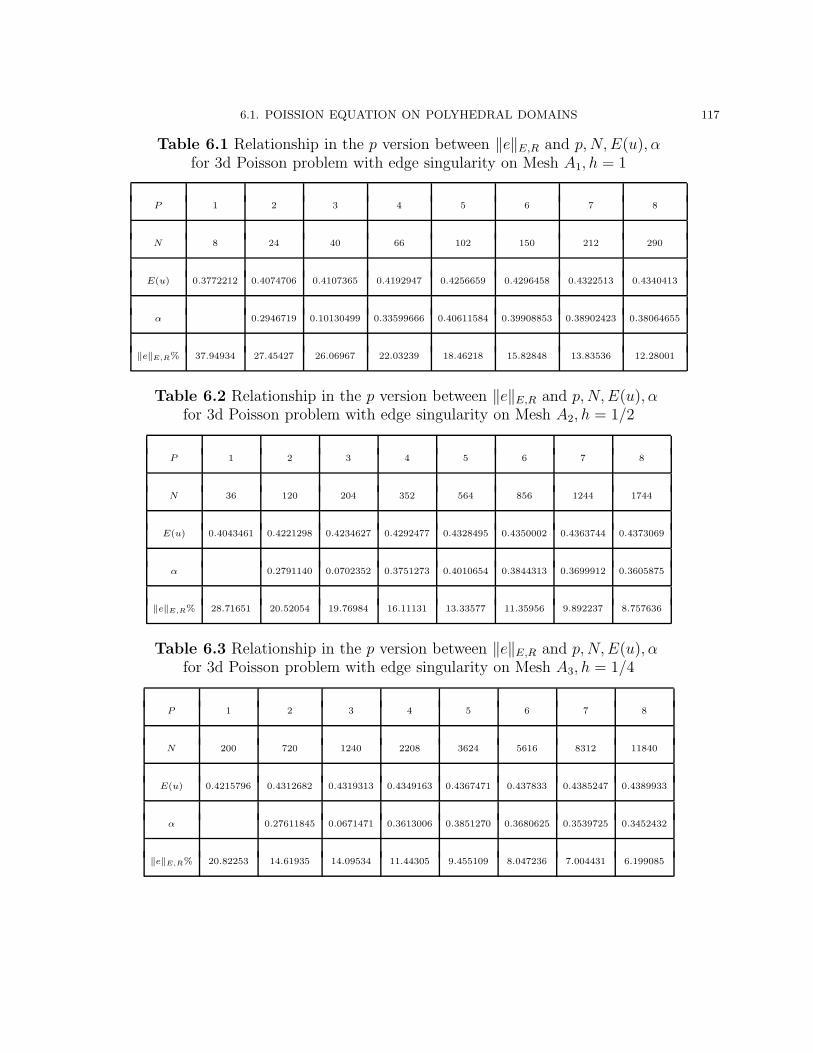
6.1. POISSION EQUATION ON POLYHEDRAL DOMAINS 117
Table 6.1 Relationship in the p version between ‖e‖E,R and p,N,E(u), αfor 3d Poisson problem with edge singularity on Mesh A1, h = 1
P 1 2 3 4 5 6 7 8
N 8 24 40 66 102 150 212 290
E(u) 0.3772212 0.4074706 0.4107365 0.4192947 0.4256659 0.4296458 0.4322513 0.4340413
α 0.2946719 0.10130499 0.33599666 0.40611584 0.39908853 0.38902423 0.38064655
‖e‖E,R% 37.94934 27.45427 26.06967 22.03239 18.46218 15.82848 13.83536 12.28001
Table 6.2 Relationship in the p version between ‖e‖E,R and p,N,E(u), αfor 3d Poisson problem with edge singularity on Mesh A2, h = 1/2
P 1 2 3 4 5 6 7 8
N 36 120 204 352 564 856 1244 1744
E(u) 0.4043461 0.4221298 0.4234627 0.4292477 0.4328495 0.4350002 0.4363744 0.4373069
α 0.2791140 0.0702352 0.3751273 0.4010654 0.3844313 0.3699912 0.3605875
‖e‖E,R% 28.71651 20.52054 19.76984 16.11131 13.33577 11.35956 9.892237 8.757636
Table 6.3 Relationship in the p version between ‖e‖E,R and p,N,E(u), αfor 3d Poisson problem with edge singularity on Mesh A3, h = 1/4
P 1 2 3 4 5 6 7 8
N 200 720 1240 2208 3624 5616 8312 11840
E(u) 0.4215796 0.4312682 0.4319313 0.4349163 0.4367471 0.437833 0.4385247 0.4389933
α 0.27611845 0.0671471 0.3613006 0.3851270 0.3680625 0.3539725 0.3452432
‖e‖E,R% 20.82253 14.61935 14.09534 11.44305 9.455109 8.047236 7.004431 6.199085

6.1. POISSION EQUATION ON POLYHEDRAL DOMAINS 118
100
101
102
103
104
105
100
101
102
A1 (h=1)
A2 (h=1/2)
A3 (h=1/4)
Relative error in energy and degrees of freedom 3d Poission problem with edge singularity on mesh A
n, n=1,2,3.
||e||E,R
%
N
Fig. 6.3 Relative error in the p version between energy norm and degreesof freedom for 3d Poission problem with edge singularity on uniform meshes

6.1. POISSION EQUATION ON POLYHEDRAL DOMAINS 119
The h version is a special case of the h-p version with fixed p. Then error estimation(6.2) is deduced to
‖e‖E,R ≤ Ch12 ≈ CN− 1
6 .(6.5)
The convergence rate α for the h version is 16. We calculate the rate for each solution of the
h version by the extrapolation similar with (6.4) except replacing up by un and Np by Nn,1 ≤ n ≤ 3.
The Table 6.4−Table 6.11 describe the performance of the h version on the uniformmeshes An, 1 ≤ n ≤ 3 with fixed degree p, 1 ≤ p ≤ 8, which show the relationship between‖e‖E,R and p, N , E(u), α for the h version. The relationship is plotted in Fig. 6.4. FromTable 6.4−Table 6.11 we can see that α asymptotically approaches its theoretical value0.1666667 as the mesh is refined and the degree increases.
Table 6.4 Relationship in the h version between ‖e‖E,R and p,N,E(u), αfor 3d Poisson problem with edge singularity for p = 1
h 1 1/2 1/4
N 8 36 200
E(u) 0.3772212 0.4043461 0.4215796
α 0.1853494 0.187448591
‖e‖E,R% 37.94934 28.71651 20.82253
Table 6.5 Relationship in the h version between ‖e‖E,R and p,N,E(u), αfor 3d Poisson problem with edge singularity for p = 2
h 1 1/2 1/4
N 24 120 720
E(u) 0.4074706 0.4221298 0.4312682
α 0.1808677 0.1892443
‖e‖E,R% 27.45427 20.52054 14.61935

6.1. POISSION EQUATION ON POLYHEDRAL DOMAINS 120
Table 6.6 Relationship in the h version between ‖e‖E,R and p,N,E(u), αfor 3d Poisson problem with edge singularity for p = 3
h 1 1/2 1/4
N 40 204 1240
E(u) 0.4107365 0.4234627 0.4319313
α 0.1697815 0.1874577
‖e‖E,R% 26.06967 19.76984 14.09534
Table 6.7 Relationship in the h version between ‖e‖E,R and p,N,E(u), αfor 3d Poisson problem with edge singularity for p = 4
h 1 1/2 1/4
N 66 352 2208
E(u) 0.4192947 0.4292477 0.4349163
α 0.1869753 0.1863289
‖e‖E,R% 22.03239 16.11131 11.44305
Table 6.8 Relationship in the h version between ‖e‖E,R and p,N,E(u), αfor 3d Poisson problem with edge singularity for p = 5
h 1 1/2 1/4
N 102 564 3624
E(u) 0.4256659 0.4328495 0.4367471
α 0.19020971 0.1848620
‖e‖E,R% 18.46218 13.33577 9.455109

6.1. POISSION EQUATION ON POLYHEDRAL DOMAINS 121
Table 6.9 Relationship in the h version between ‖e‖E,R and p,N,E(u), αfor 3d Poisson problem with edge singularity for p = 6
h 1 1/2 1/4
N 150 856 5616
E(u) 0.4296458 0.4350002 0.437833
α 0.1904828 0.1832596
‖e‖E,R% 15.82848 11.35956 8.047236
Table 6.10 Relationship in the h version between ‖e‖E,R and p,N,E(u), αfor 3d Poisson problem with edge singularity for p = 7
h 1 1/2 1/4
N 212 1244 8312
α 0.1895886 0.1817485
E(u) 0.4322513 0.4363744 0.4385247
‖e‖E,R% 13.83536 9.892237 7.004431
Table 6.11 Relationship in the h version between ‖e‖E,R and p,N,E(u), αfor 3d Poisson problem with edge singularity for p = 8
h 1 1/2 1/4
N 290 1744 11840
E(u) 0.4340413 0.4373069 0.4389933
α 0.1884261 0.1804020
‖e‖E,R% 12.28001 8.757636 6.199085

6.1. POISSION EQUATION ON POLYHEDRAL DOMAINS 122
100
101
102
103
104
105
100
101
102
p=1p=2p=3p=4p=5p=6p=7p=8
Relative error in energy and degrees of freedom 3d Poission problem with edge singularity h−version on uniform mesh A
n, n=1,2,3.
||e||E,R
%
N
Fig. 6.4 Relative error in the h version between energy norm and degrees of freedomfor 3d Poission problem with edge singularity on uniform meshes An, 1 ≤ n ≤ 3.

6.1. POISSION EQUATION ON POLYHEDRAL DOMAINS 123
The h-p version reduces the element size h and increase the degree p simultaneously toreduce quickly the error by less computation. The performance of the h-p version on uniformmeshes An, n = 1, 2, 3 associated with p = 2, 3, 4 is given in Table 6.12 and Fig. 6.7.
Table 6.12 Relationship in the h-p version between ‖e‖E,R, p, N,E(u)for 3d Poisson problem with edge singularity on uniform mesh An.
Mesh h p N E(u) α ‖e‖E,R%
A1 1 2 24 0.4074706 27.45
A212
3 204 0.4234627 0.1534364 19.77
A314
4 2208 0.4349163 0.2295714 11.44
101
102
103
104
101
Relative error in energy and degrees of freedom for h−p version3d Poission problem with edge singularity on uniform mesh A
n, 1 ≤ n ≤ 3.
||e||E,R
%
Mesh A1, P=2
Mesh A2, P=3
Mesh A3, P=4
N
Fig. 6.5 Relative error in the h-p version between energy norm and degreesof freedom for 3d Poission problem with edge singularity on uniform meshes
The computation results in Table 6.1−Table 6.12 show that the theory of finite elementmethod for edge-singular functions is very reliable and coincides with the computation.

6.1. POISSION EQUATION ON POLYHEDRAL DOMAINS 124
The computations are done also on geometric meshes Bn, 1 ≤ n ≤ 6 with mesh factorσ = 0.15 shown in Fig. 6.3. and Fig. 6.4.
x1
x2
x3
x1
x2
x3
x3
x2
x1
x2
x3
σ5
x2
x3
x1
x1
x2
x3
o o σMesh B
o σσ 2 x1
σo σ4
σo
σo σ 3
Mesh B Mesh B
Mesh B Mesh B
Mesh B1 2
4
65
3
Fig. 6.6 Geometric meshes Bn, 1 ≤ n ≤ 6
Table 6.13−Table 6.17 show the relationship between ‖e‖E,R and p,N ,E(u),α for p ver-sion. The relationship are plotted in Fig. 6.8. Due to (6.3), the rate of convergence isasymptotically α = 1
3≈ 0.3333333. Table 6.13−Table 6.17 and Fig. 6.8. indicate that the p
version on the geometric meshes Bn, 1 ≤ n ≤ 6 with increasing p perform in pre-asymptoticrange and α calculated by (6.4) is bigger than the asymptotic value, which make the p

6.1. POISSION EQUATION ON POLYHEDRAL DOMAINS 125
version on the geometric meshes Bn more effective than on uniform meshes An. The over-refined meshes balance the strong edge singularity on the x3-axis where the elements size isreduced dramatically to 0.15n−1 and delay significantly entering the asymptotical range ofthe p version.
Table 6.13 Relationship in the p version between ‖e‖E,R and p,N,E(u)for 3d Poisson problem with edge singularity on geometric mesh B2
P 1 2 3 4 5 6 7 8
N 16 52 88 150 238 358 516 718
E(u) 0.4127698 0.4330268 0.4349613 0.4371067 0.4382714 0.4389508 0.4393763 0.4396627
α 0.5486015 0.2766451 0.4402217 0.4262301 0.4044964 0.3845665 0.3732178
‖e‖E,R% 25.1692 13.18407 11.39834 9.013274 7.403371 6.276389 5.453226 4.820656
Table 6.14 Relationship in the p version between ‖e‖E,R and p,N,E(u)for 3d Poisson problem with edge singularity on geometric mesh B3
P 1 2 3 4 5 6 7 8
N 24 80 136 234 374 566 820 1146
E(u) 0.4191359 0.4379563 0.4396005 0.4401144 0.4403182 0.4404250 0.4404898 0.440533
α 0.8579649 0.8685056 0.5903211 0.4692828 0.4128646 0.3835571 0.3697782
‖e‖E,R% 22.11402 7.871474 4.964893 3.604 2.892096 2.437361 2.114307 1.868156

6.1. POISSION EQUATION ON POLYHEDRAL DOMAINS 126
Table 6.15 Relationship in the p version between ‖e‖E,R and p,N,E(u)for 3d Poisson problem with edge singularity on geometric mesh B4
P 1 2 3 4 5 6 7 8
N 32 108 184 318 510 774 1124 1574
E(u) 0.4204377 0.4387308 0.4403132 0.4405695 0.4406265 0.4406467 0.4406571 0.4406637
α 0.9607110 1.5535445 1.0586893 0.7043395 0.4889666 0.4023689 0.3731730
‖e‖E,R% 21.43571 6.662227 2.911645 1.631488 1.169752 0.953909 0.820943 0.724004
Table 6.16 Relationship in the p version between ‖e‖E,R and p,N,E(u)for 3d Poisson problem with edge singularity on geometric mesh B5
P 1 2 3 4 5 6 7 8
N 40 136 232 402 646 982 1428 2002
E(u) 0.4206717 0.4388525 0.440421 0.4406379 0.4406728 0.44068 0.4406822 0.4406833
α 0.9764145 1.8084042 1.5398594 1.3183587 0.8621643 0.5219361 0.4044335
‖e‖E,R% 21.31149 6.451641 2.45591 1.053391 0.563636 0.392816 0.323083 0.281818
Table 6.17 Relationship in the p version between ‖e‖E,R and p,N,E(u)for 3d Poisson problem with edge singularity on geometric mesh B6
P 1 2 3 4 5 6 7 8
N 48 164 280 486 782 1190 1732 2430
E(u) 0.4207152 0.4388714 0.4404373 0.4406481 0.4406797 0.4406849 0.4406860 0.4406862
α 0.9758578 1.8550348 1.6898395 1.7825698 1.5698807 1.1523358 0.4247930
‖e‖E,R% 21.28832 6.418317 2.379415 0.93711 0.401388 0.20764 0.134735 0.116684

6.1. POISSION EQUATION ON POLYHEDRAL DOMAINS 127
100
101
102
103
104
10−1
100
101
102
B1
B2
B3
B4
B5
B6
Relative error in energy and degrees of freedom for the p version3d Poission problem with edge singularity on geometric mesh B
n, 1 ≤ n ≤ 6.
||e||E,R
%
N
Fig. 6.7 Relationship in the p version between ‖e‖E,R and p,N,E(u)for 3d Poisson problem with edge singularity on geometric mesh Bn, 1 ≤ n ≤ 6

6.1. POISSION EQUATION ON POLYHEDRAL DOMAINS 128
The h-p version on the geometric meshes simultaneously refines the meshes by a meshfactor σ = 0.15 and increases the degree p to achieve the high accuracy with less totalnumber of freedom N . It was indicated in [26, 27] that the finite element solution of h-pversion converges exponentially,
‖e‖E ≤ c e−bN14
where constants b and c depend on the singularity of u and mesh factor σ but not on N .The performances of the h-p version on the meshes Bn with the degree p = n, 1 ≤ n ≤ 6 isillustrated in Table 6.18 and Fig. 6.9, which show that the exponential rate is achieved aspredicted by the theory.
Table 6.18 Relationship in the h-p version between ‖e‖E,R, p, N,N1/4, E(u)
for 3d Poisson problem with edge singularity on geometric mesh Bn, 1 ≤ n ≤ 6
Mesh P N N1/4 E(u) ‖e‖E,R% b c
B1 1 8 1.6818 0.3772212 37.94934
B2 2 52 2.6853 0.4330268 13.18407 2.1144860 0.5980102
B3 3 136 3.4150 0.4396005 4.964893 1.9532346 0.4438187
B4 4 318 4.2229 0.4405695 1.631488 2.2257980 0.9672330
B5 5 646 5.0415 0.4406728 0.563636 1.99858 0.6564106
B6 6 1190 5.8734 0.4406849 0.20764 1.8513516 0.3518381
In Table 6.18 b and c are calculated by extrapolation, i.e.,
b = ln∆(p)
∆(p+ 1), c =
∆(p)(
∆(p)∆(p+1)
)(1 − ∆(p+1)
∆(p)
)
∆(p) = E(up+1) − E(up).

6.1. POISSION EQUATION ON POLYHEDRAL DOMAINS 129
1 2 3 4 5 6 710
−1
100
101
102
Relative error in energy and degrees of freedom for h−p version3d Poission problem with edge singularity on geometric mesh B
n, 1 ≤ n ≤ 6.
||e||E,R
%
Mesh B1, P=1
Mesh B2, P=2
Mesh B3, P=3
Mesh B4, P=4
Mesh B5, P=5
Mesh B6, P=6
N1/4
Fig. 6.8 Relationship in the h-p version between ‖e‖E,R, p, N,N1/4, E(u)
for 3d Poisson problem with edge singularity on geometric mesh Bn, 1 ≤ n ≤ 6
6.1.2. Poisson equation with vertex-edge singularity. Next we solve the followingPoisson problem:
(6.6)
−u = −2ρ12 sin
12 θ sin φ
2in D = [−1, 1] × [0, 1] × [0, 1],
u∣∣Γ2
= u∣∣Γ1
= u∣∣Γ4
= 0,∂u∂n
∣∣Γ1
= ∂u∂n
∣∣Γ4
= ∂u∂n
∣∣Γ7
= 0,∂u∂n
∣∣Γ3
= 12ρ
12 sin− 1
2 θ cos θ(ρ cos θ − 1) sin φ2,
∂u∂n
∣∣Γ6
= −12ρ
12 sin− 1
2 θ cos θ(ρ cos θ − 1) sin φ2,
∂u∂n
∣∣Γ5
= 12ρ
12 sin− 1
2 θ cos θ(ρ cos θ − 1) cos φ2
where the domain D for the problem is shown in Fig. 6.1 , and Γ1,Γ2, · · · ,Γ7 are facesof D, Γ1 : x3 = 0, Γ4 : x3 = 1; Γ2 : x2 = 0, 0 ≤ x1 ≤ 1, Γ7 : x2 = 0,−1 ≤ x1 ≤ 0,Γ5 : x2 = 1; Γ3 : x1 = −1, Γ6 : x1 = 1,
ρ =√x2
1 + x22 + x2
3, r =√x2
1 + x22, θ = arctan
r
x3
, φ = arcsinx2
r.
It is known that
u = ρ12 sin
12 θ sin
φ
2.

6.1. POISSION EQUATION ON POLYHEDRAL DOMAINS 130
is the exact solution of the problem (6.6), and the strain energy of u.
E(u) =1
2B(u, u) =
1
2
∫
D
[( ∂u
∂x1
)2
+( ∂u
∂x2
)2
+( ∂u
∂x3
)2]dx1dx2dx3
≈ 0.14222217919263.
The finite element solution of the h, p and h-p version computed on uniform meshes An, 1 ≤n ≤ 3 with h = 1, 1/2 and 1/4 shown in Fig. 6.2.
The solution has the singularity of ργ sinσ θ-type with γ = σ = 1/2. According toTheorem 5.20, there holds for the solution of h-p version
‖e‖E,R ≤ Ch
12
p.(6.7)
The p version is a special case of the h-p version with fixed h. Then error estimation isdeduced to
‖e‖E,R ≤ Cp−1 ≈ CN− 13 .(6.8)
Hereafter N denotes the number of degrees of freedom for finite element spaces, which thethe number of unknown of the resulting system of linear algebraic equations.
Table 6.19−Table 6.21 show the relationship between ‖e‖E,R and p, N , E(u), α for thep version on each fixed mesh An. The relationship are plotted in Fig. 6.9. Due to (6.8) therate of convergence is 1
3. We calculate the convergence rate for each finite element of the p
version by the extrapolation [45],
α =log E(u)−E(up)
E(u)−E(up+1)
2 logNp+1
Np
.(6.9)
where up is finite element solution of the p version with degree p and Np denotes the corre-sponding total number of the freedom.
From Table 6.19−Table 6.21 we can see that α asymptotically approaches to the the-oretical value 1/3 as the degree p increases and the meshes are refined. The computationindicates that the convergence rate of the p version with the degree 1 ≤ p ≤ 8 on theseuniform meshes associated is in pre-asymptotical range and higher than asymptotical value.

6.1. POISSION EQUATION ON POLYHEDRAL DOMAINS 131
Table 6.19 Relationship in the p version between ‖e‖E,R and p,N,E(u)for 3d Poisson problem with vertex-edge singularity on Mesh A1, h = 1
P 3 4 5 6 7 8
N 8 18 34 58 92 138
E(u) 0.1382483 0.1408121 0.1410113 0.1414079 0.1416734 0.1418290
α 0.6388323 0.1197342 0.3714769 0.4276698 0.4111706
‖e‖E,R% 16.71567 9.95722 9.227132 7.566639 6.211767 5.257891
Table 6.20 Relationship in the p version between ‖e‖E,R and p,N,E(u)for 3d Poisson problem with vertex-edge singularity on Mesh A2, h = 1/2
P 1 2 3 4 5 6 7 8
N 12 56 100 192 332 536 820 1200
E(u) 0.1084475 0.1414734 0.1415308 0.1418040 0.1419372 0.1420201 0.1420714 0.1421052
α 1.2363383 0.0687764 0.3853741 0.3501334 0.3588278 0.3443835 0.3332966
‖e‖E,R% 48.73174 7.255932 6.972275 5.422475 4.476338 3.769443 3.25602 2.867944
Table 6.21 Relationship in the p version between ‖e‖E,R and p,N,E(u)for 3d Poisson problem with vertex-edge singularity on Mesh A3, h = 1/4
P 1 2 3 4 5 6 7 8
N 120 496 872 1632 2776 4432 6728 9792
E(u) 0.1335454 0.1418894 0.1419145 0.1420234 0.1420877 0.1421254 0.1421492 0.1421652
α 1.1489546 0.069496323 0.3485023 0.3678291 0.3515919 0.3380923 0.3297312
‖e‖E,R% 24.69992 4.837204 4.651204 3.738538 3.074991 2.608599 2.265249 2.001587

6.1. POISSION EQUATION ON POLYHEDRAL DOMAINS 132
1 10 100 1000 1500010
0
101
102
A1(h=1)
A2(h=1/2)
A3(h=1/4)
Relative error in energy and degrees of freedom for the pversion3d Poission problem with vertex−edge singularity on Mesh A
n, n=1,2,3.
||e||E,R
%
N
Fig. 6.9 Relative error in the p version between energy norm and degrees of freedomfor 3d Poission problem with vertex-edge singularity on uniform meshes

6.1. POISSION EQUATION ON POLYHEDRAL DOMAINS 133
The h version is a special case of the h-p version with fixed p. Then error estimation(6.7) is deduced to
‖e‖E,R ≤ Ch12 ≈ CN− 1
6 .(6.10)
The convergence rate α for the h version is 16. We calculate the rate for each solution of the
h version by the extrapolation similar with (6.9) except replacing up by un and Np by Nn,1 ≤ n ≤ 3.
The Table 6.22−Table 6.28 describe the performance of the h version on the uniformmeshes An, 1 ≤ n ≤ 3 with fixed degree p, 1 ≤ p ≤ 8, which show the relationship between‖e‖E,R and p, N , E(u), α for the h version. The relationship is plotted in Fig. 6.10. FromTable 6.22−Table 6.28 we can see that α asymptotically approaches its theoretical value0.1666667 as the mesh is refined and the degree increases.
Table 6.22 Relationship in the h version between ‖e‖E,R and p,N,E(u)for 3d Poisson problem with vertex-edge singularity for p = 2
h 1 1/2 1/4
N 4 56 496
E(u) 0.1382354 0.1414734 0.1418894
α 0.3168355 0.1858964
‖e‖E,R% 16.74277 7.255932 4.837204
Table 6.23 Relationship in the h version between ‖e‖E,R and p,N,E(u)for 3d Poisson problem with vertex-edge singularity for p = 3
h 1 1/2 1/4
N 8 100 872
E(u) 0.1382483 0.1415308 0.1419145
α 0.3461988 0.1869279
‖e‖E,R% 16.71567 6.972275 4.651204
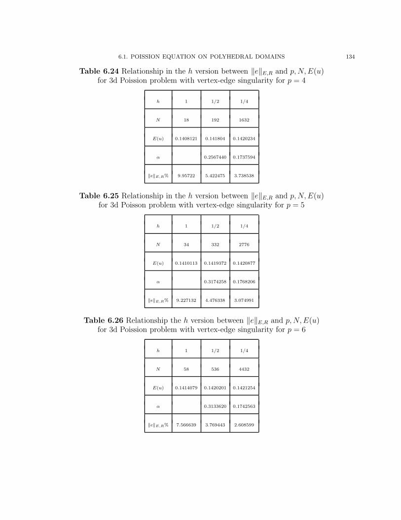
6.1. POISSION EQUATION ON POLYHEDRAL DOMAINS 134
Table 6.24 Relationship in the h version between ‖e‖E,R and p,N,E(u)for 3d Poission problem with vertex-edge singularity for p = 4
h 1 1/2 1/4
N 18 192 1632
E(u) 0.1408121 0.141804 0.1420234
α 0.2567440 0.1737594
‖e‖E,R% 9.95722 5.422475 3.738538
Table 6.25 Relationship in the h version between ‖e‖E,R and p,N,E(u)for 3d Poisson problem with vertex-edge singularity for p = 5
h 1 1/2 1/4
N 34 332 2776
E(u) 0.1410113 0.1419372 0.1420877
α 0.3174258 0.1768206
‖e‖E,R% 9.227132 4.476338 3.074991
Table 6.26 Relationship the h version between ‖e‖E,R and p,N,E(u)for 3d Poission problem with vertex-edge singularity for p = 6
h 1 1/2 1/4
N 58 536 4432
E(u) 0.1414079 0.1420201 0.1421254
α 0.3133620 0.1742563
‖e‖E,R% 7.566639 3.769443 2.608599
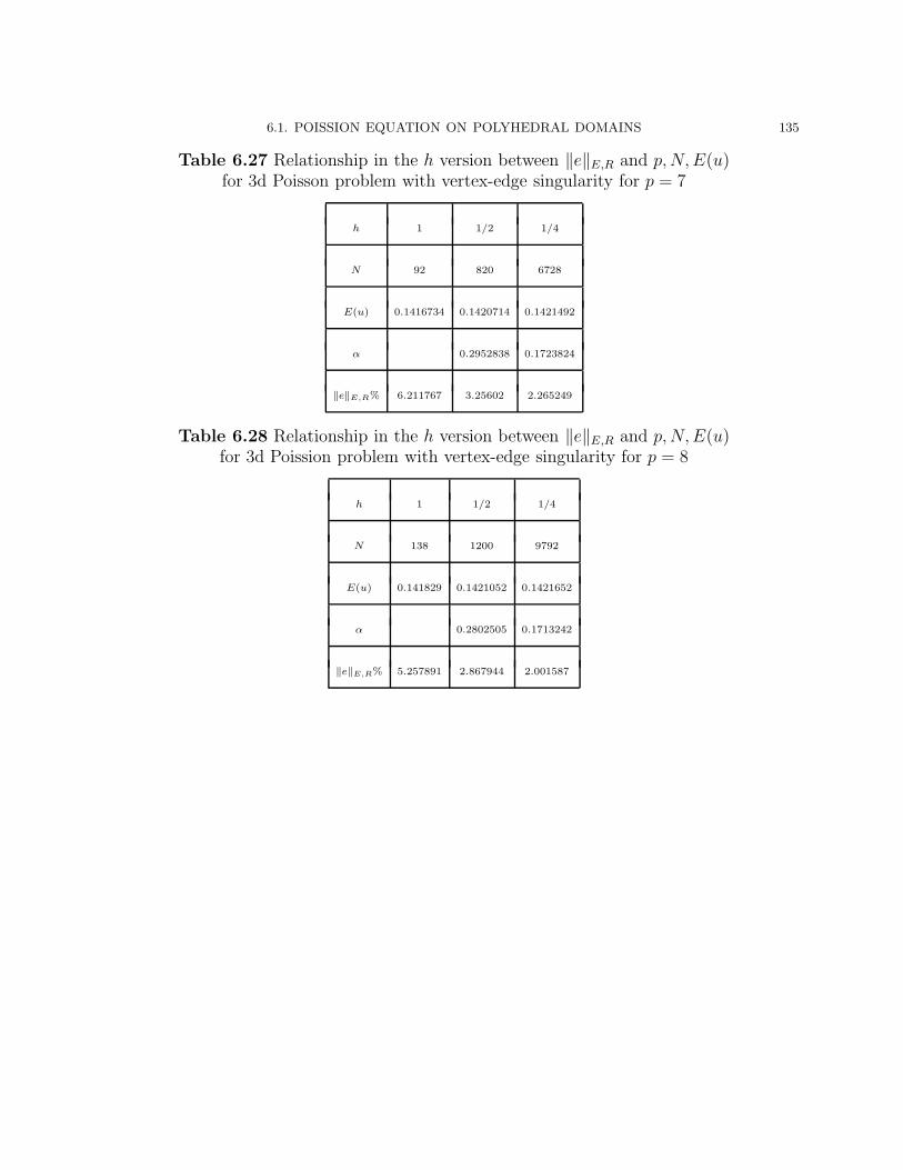
6.1. POISSION EQUATION ON POLYHEDRAL DOMAINS 135
Table 6.27 Relationship in the h version between ‖e‖E,R and p,N,E(u)for 3d Poisson problem with vertex-edge singularity for p = 7
h 1 1/2 1/4
N 92 820 6728
E(u) 0.1416734 0.1420714 0.1421492
α 0.2952838 0.1723824
‖e‖E,R% 6.211767 3.25602 2.265249
Table 6.28 Relationship in the h version between ‖e‖E,R and p,N,E(u)for 3d Poission problem with vertex-edge singularity for p = 8
h 1 1/2 1/4
N 138 1200 9792
E(u) 0.141829 0.1421052 0.1421652
α 0.2802505 0.1713242
‖e‖E,R% 5.257891 2.867944 2.001587

6.1. POISSION EQUATION ON POLYHEDRAL DOMAINS 136
100
101
102
103
104
100
101
102
p=3p=4p=5p=6p=7p=8
Relative error in energy and degrees of freedom for the h−version3d Poission problem with vertex−edge singularity on mesh A
n, n=1,2,3.
||e||E,R
%
N
Fig. 6.10 Relative error in the h version between energy norm and degreesof freedom for 3d Poission problem with vertex-edge singularity on uniform meshes

6.2. THREE DIMENSIONAL ELASTICITY PROBLEMS ON POLYHEDRAL DOMAINS 137
The h-p version reduces the element size h and increase the degree p simultaneously toreduce quickly the error by less computation. The performance of the h-p version on uniformmeshes An, n = 1, 2, 3 associated with p = 2, 3, 4 is given in Table 6.29 and Fig. 6.11.
Table 6.29 Relationship in the h-p version between ‖e‖E,R, p, N,N1/4, E(u)
for 3d Poisson problem with edge singularity on uniform mesh An.
Mesh h p N N1/4 E(u) α ‖e‖E,R%
A1 1 2 4 1.4142 0.1382354 16.74277
A212
3 100 3.1623 0.1415308 0.2721524 6.972275
A314
4 1632 6.3559 0.1420234 0.2231942 3.738538
1 2 3 4 5 6 7
101
Relative error in energy and degrees of freedom for h−p version3d Poission problem with vertex−edge singularity on uniform mesh A
n, 1≤ n ≤ 3.
||e||E,R
%
Mesh A1, P=2
Mesh A2, P=3
Mesh A3, P=4
N
Fig. 6.11 Relative error in the h-p version between energy norm and degrees of freedomfor 3d Poisson problem with vertex-edge singularity on uniform mesh An, 1 ≤ n ≤ 3.
The computation results in Table 6.19−Table 6.29 show that the theory of finite elementmethod for vertex-edge singular functions is very reliable and coincides with the computation.
6.2. Three dimensional elasticity problems on polyhedral domains
In this section, we will solve three dimensional elasticity problems(homogeneous isotropicmaterial) on polyhedral domains. We denote the Young’s modulus of elasticity and Poissonratio respectively by E and ν. The domain Ω is shown in Fig. 6.12.

6.2. THREE DIMENSIONAL ELASTICITY PROBLEMS ON POLYHEDRAL DOMAINS 138
Let u = (u1, u2, u3) be the displacement vector, and let σ be the stress tensor and T bethe traction vector.
σ11 = λ(∂u1
∂x1+∂u2
∂x2+∂u3
∂x3
)+ 2µ
∂u1
∂x1
σ22 = λ(∂u1
∂x1+∂u2
∂x2+∂u3
∂x3
)+ 2µ
∂u2
∂x2
σ33 = λ(∂u1
∂x1+∂u2
∂x2+∂u3
∂x3
)+ 2µ
∂u3
∂x3
and
σ23 = µ(∂u2
∂x3+∂u3
∂x2
)
σ31 = µ(∂u3
∂x1
+∂u1
∂x3
)
σ12 = µ(∂u1
∂x2
+∂u2
∂x1
).
where λ = Eν(1+ν)(1−2ν)
and µ = E2(1+ν)
, µ is the conventional shear modulus.
We consider the three dimensional elasticity problem for E = 100 and ν = 0.3:
(λ+ µ)∂
∂x1
(∂u1
∂x1+∂u2
∂x2+∂u3
∂x3
)+ µ∇2u1 = 0,
(λ+ µ)∂
∂x2
(∂u1
∂x1+∂u2
∂x2+∂u3
∂x3
)+ µ∇2u2 = 0,
(λ+ µ)∂
∂x3
(∂u1
∂x1
+∂u2
∂x2
+∂u3
∂x3
)+ µ∇2u3 = 0
(6.11)
with boundary conditions:
u1 = 0, T2 = T3 = 0 on Γ1 = (0, x2, x3)| 0 ≤ x2 ≤ 1, 0 ≤ x3 ≤ 1,u2 = 0, T1 = T3 = 0 on Γ2 = (x1, 0, x3)| 0 ≤ x1 ≤ 1, 0 ≤ x3 ≤ 1,u3 = 0, T1 = T2 = 0 on Γ3 = (x1, x2, 0)| 0 ≤ x1 ≤ 1, 0 ≤ x2 ≤ 1,
Γ4 = (x1, x2,12)| 0 ≤ x1 ≤ 1
2, 0 ≤ x2 ≤ 1
2,
T1 = T2 = T3 = 0 on Γ5 = (12, x2, x3)| 0 ≤ x2 ≤ 1
2, 1
2≤ x3 ≤ 1,
Γ6 = (x1,12, x3)| 0 ≤ x1 ≤ 1
2, 1
2≤ x3 ≤ 1,
Γ7 = (1, x2, x3)| 0 ≤ x2 ≤ 1, 0 ≤ x3 ≤ 1,Γ8 = (x1, 1, x3)| 0 ≤ x1 ≤ 1, 0 ≤ x3 ≤ 1,
T1 = T2 = 0, T3 = 2 on Γ9 = (x1, x2, 1)| 12≤ x2 ≤ 1 for 0 ≤ x1 ≤ 1
2,
and 0 ≤ x2 ≤ 1 for 12≤ x1 ≤ 1.
(6.12)
In this problem, we do not know the exact solution and the strain energy of the problem.
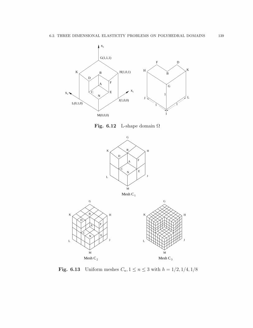
6.2. THREE DIMENSIONAL ELASTICITY PROBLEMS ON POLYHEDRAL DOMAINS 139
x3
M(0,0,0)
J(1,0,0)
A
EN
C x
F
B
D
L(0,1,0)
K
G(1,1,1)
H(1,0,1)
G
H
F
B
D
J
K
1
I
L
1 1
x21
Fig. 6.12 L-shape domain Ω
Mesh C2
Mesh C1
Mesh C3
K
L
M
J
H
G
A
NC
F
D
K
E
B
L
M
J
H
G
A
NC
F
D
K
E
B
L
M
J
H
G
Fig. 6.13 Uniform meshes Cn, 1 ≤ n ≤ 3 with h = 1/2, 1/4, 1/8

6.2. THREE DIMENSIONAL ELASTICITY PROBLEMS ON POLYHEDRAL DOMAINS 140
The computation of the h, p and h-p version have been done on uniform mesh Cn withsquare elements, 1 ≤ n ≤ 3, shown on Fig. 6.13, by the commercial codes StressCheck V7.1developed by ESRD Inc. and ProPHLEX developed by Altair Engineering Inc.
Table 6.30−Table 6.32 show the relationship between ‖e‖E,R and p, N , E(u), α in the pversion on each fixed mesh Cn, 1 ≤ n ≤ 3. The relationship are plotted in Fig. 6.14.
We calculate the convergence rate for each finite element solution by the extrapolation[45].
E(u) is the root of the equation
F (E(u)) =E(u) −E(u2)
E(u) −E(u3)−
(E(u) −E(u1)
E(u) −E(u2)
)Q
= 0
where Q =log
N3N2
logN2N1
with Ni, i = 1, 2, 3 denotes the degree of freedom corresponding to the
finite element space. E(u) can be solved by Newton’s iteration method or other numericalmethod, and denoted by E(u) to distinguish the energy E(u) of exact solution.
Once E(u) is solved, we can determine the exponent α by
α ≈ logF2,3
2 log N3
N2
=log E(u)−E(u2)
E(u)−E(u3)
2 log N3
N2
.
In Fig. 6.14 the error curves for the p-version on the mesh Cn, n = 1, 2, 3 plotted inlog-log scale are very close to straight line which are parallel and the slope is the rate of theconvergence. Obviously, the solution has singularity at the vertex A = (1
2, 1
2, 1
2) and on the
edge AB,AC and AE. The strongest singularity occurs along the edge AC = (x1,12, 1
2)|0 ≤
x1 ≤ 12 and AE = (1
2, x2,
12)|0 ≤ x2 ≤ 1
2. It seems the rate α of the convergence is around
0.3 ∼ 0.4, which is predicted as 23min(γ + 1
2, σ), where γ is the vertex singularity and σ is
the edge singularity.
Table 6.30 Relationship in the p version between ‖e‖E,R and p,N,E(u), αfor 3d elasticity problem on Mesh C1, h = 1/2
P 1 2 3 4 5 6 7 8
N 49 275 803 1759 3269 5459 8455 12383
E(u) 0.01193771 0.01287213 0.01313627 0.01325604 0.01332475 0.01336881 0.01339907 0.01342105
α 0.2531353 0.5469898 0.5096197 0.4536066 0.4483468 0.4552743 0.4457332
‖e‖E,R% 34.40 22.20 17.26 14.47 12.60 11.23 10.19 9.36

6.2. THREE DIMENSIONAL ELASTICITY PROBLEMS ON POLYHEDRAL DOMAINS 141
Table 6.31 Relationship in the p version between ‖e‖E,R and p,N,E(u), αfor 3d elasticity problem on Mesh C2, h = 1/4
P 1 2 3 4 5 6 7 8
N 275 1759 5459 12383 23539 39935 62579 92479
E(u) 0.01262429 0.01314234 0.01329410 0.01336622 0.01340775 0.01343445 0.01345291 0.01346635
α 0.2239465 0.4775917 0.4256249 0.4201082 0.4199877 0.4207112 0.4219232
‖e‖E,R% 26.02 17.17 13.52 11.38 9.94 8.89 8.09 7.45
Table 6.32 Relationship in the p version between ‖e‖E,R and p,N,E(u), αfor 3d elasticity problem on Mesh C3, h = 1/8
P 1 2 3 4 5 6
N 1746 12351 39876 92385 177942 304611
E(u) 0.01300402 0.01329891 0.01338862 0.01343203 0.01345726 0.01347357
α 0.2029820 0.4216856 0.3865125 0.3913336 0.3973223
‖e‖E,R% 19.94 13.40 10.65 9.02 7.92 7.12

6.2. THREE DIMENSIONAL ELASTICITY PROBLEMS ON POLYHEDRAL DOMAINS 142
101
102
103
104
105
106
100
101
102
C1(h=1/2)
C2(h=1/4)
C3(h=1/8)
Relative Error in the p version between energy and degrees of freedom for 3d elasticity problem on uniform mesh C
n, 1 ≤ n ≤ 3.
||e||%
Fig. 6.14 Relative error in the p version between energy normand degrees of freedom for 3d elasticity problem on uniform meshes

6.2. THREE DIMENSIONAL ELASTICITY PROBLEMS ON POLYHEDRAL DOMAINS 143
The Table 6.33−Table 6.38 describe the performance of the h version on the uniformmeshes Cn, 1 ≤ n ≤ 3 with fixed degree p, 1 ≤ p ≤ 8, which show the relationship between‖e‖E,R and p, N , E(u), α in the h version. The relationship is plotted in Fig. 6.15.
Table 6.33 Relationship in the h version between ‖e‖E,R and p,N,E(u), αfor 3d elasticity problem for p = 1
h 1/2 1/4 1/8
N 49 275 1746
E(u) 0.01193771 0.01262429 0.01300402
α 0.3237904 0.3715672
‖e‖E,R% 34.40 26.02 19.94
Table 6.34 Relationship in the h version between ‖e‖E,R and p,N,E(u), αfor 3d elasticity problem for p = 2
h 1/2 1/4 1/8
N 275 1759 12351
E(u) 0.01287213 0.01314234 0.01329891
α 0.2782727 0.3133864
‖e‖E,R% 22.20 17.17 13.40

6.2. THREE DIMENSIONAL ELASTICITY PROBLEMS ON POLYHEDRAL DOMAINS 144
Table 6.35 Relationship in the h version between ‖e‖E,R and p,N,E(u), αfor 3d elasticity problem for p = 3
h 1/2 1/4 1/8
N 803 5459 39876
E(u) 0.01313627 0.01329410 0.01338862
α 0.2569841 0.2818973
‖e‖E,R% 17.26 13.52 10.65
Table 6.36 Relationship the h version between ‖e‖E,R and p,N,E(u), αfor 3d elasticity problem for p = 4
h 1/2 1/4 1/8
N 1759 12383 92385
E(u) 0.01325604 0.01336622 0.01343203
α 0.2492676 0.2753614
‖e‖E,R% 14.47 11.38 9.02
Table 6.37 Relationship in the h version between ‖e‖E,R and p,N,E(u), αfor 3d elasticity problem for p = 5
h 1/2 1/4 1/8
N 3269 23539 177942
E(u) 0.01332475 0.01340775 0.01345726
α 0.2437201 0.2709999
‖e‖E,R% 12.60 9.94 7.92

6.2. THREE DIMENSIONAL ELASTICITY PROBLEMS ON POLYHEDRAL DOMAINS 145
Table 6.38 Relationship in the h version between ‖e‖E,R and p,N,E(u), αfor 3d elasticity problem for p = 6
h 1/2 1/4 1/8
N 5459 39935 304611
E(u) 0.01336881 0.01343445 0.01347357
α 0.2392914 0.2679601
‖e‖E,R% 11.23 8.89 7.12
101
102
103
104
105
106
100
101
102
p=1p=2p=3p=4p=5p=6
Relative error in energy and degrees of freedom 3d elasticity problem h−version on uniform mesh C
n, n=1,2,3.
||e||E,R
%
N
Fig. 6.15 Relative error in the h version between energy normand degrees of freedom for 3d elasticity problem on uniform meshes

6.2. THREE DIMENSIONAL ELASTICITY PROBLEMS ON POLYHEDRAL DOMAINS 146
The h-p version reduces the element size h and increase the degree p simultaneously toreduce quickly the error by less computation. The performance of the h-p version on uniformmeshes Cn, n = 1, 2, 3 associated with p = 2, 3, 4 is given in Table 6.39 and Fig. 6.16.
Table 6.39 Relationship in the h-p version between ‖e‖E,R, p, N,E(u), αfor 3d elasticity problem on uniform mesh Cn.
Mesh h p N E(u) α ‖e‖E,R%
C112
2 275 0.01287213 22.24208
C214
3 5459 0.01329410 0.1662981 13.53185
C318
4 92385 0.01343203 0.1436109 9.014316
102
103
104
105
100
101
102
Relative error in energy and degrees of freedom for h−p version3d elasticity problem on uniform mesh C
n, 1 ≤ n ≤ 3.
||e||E,R%
Mesh C1, P=2
Mesh C2, P=3
Mesh C3, P=4
N
Fig. 6.16 Relative error in the h-p version between energy norm and degreesof freedom for 3d elasticity problem on uniform meshes
In the above computation, the product polynomial space P2p (Ωi) are adopted on each
square element. We also conducted the computation on trunk space Pκp (Ωi), 1 < κ < 2. Table
6.40−Table 6.42 show that the degree of freedom reduced significantly without compromisingthe convergence as predicted by the theorems in previous chapter.

6.2. THREE DIMENSIONAL ELASTICITY PROBLEMS ON POLYHEDRAL DOMAINS 147
Table 6.40 Relationship in the p version (trunk space) between ‖e‖E,R andp,N,E(u) for 3d elasticity problem on Mesh C1, h = 1/2
P 1 2 3 4 5 6 7 8
N 49 166 283 488 781 1183 1715 2398
E(u) 0.01193771 0.01269697 0.01279953 0.01294672 0.01307518 0.01316207 0.01322776 0.01327642
‖e‖E,R% 34.14 24.57 22.97 20.46 17.99 16.10 14.52 13.22
Table 6.41 Relationship in the p version (trunk space) between ‖e‖E,R andp,N,E(u) for 3d elasticity problem on Mesh C2, h = 1/4
P 1 2 3 4 5 6 7 8
N 275 987 1699 3015 4935 7627 11259 15999
E(u) 0.01262429 0.01303359 0.01308542 0.01318434 0.01325984 0.01331346 0.01335256 0.01338169
‖e‖E,R% 25.85 19.12 18.09 15.94 14.08 12.60 11.39 10.40
Table 6.42 Relationship in the p version (trunk space) between ‖e‖E,R andp,N,E(u) for 3d elasticity problem with edge singularity on Mesh C3, h = 1/8
P 1 2 3 4 5 6 7 8
N 1757 6608 11459 20747 34472 53978 80609 115709
E(n) 0.01359820 0.01386188 0.01389421 0.01395551 0.01400238 0.01403526 0.01405908 0.01407670
‖e‖E,R% 19.96 14.57 13.76 12.09 10.63 9.48 8.54 7.78

CHAPTER 7
Conclusion
In this thesis, we have introduced the Jacobi-weighted Besov and Sobolev spaces on scaledcube Qh = (−h, h)3 and analyzed the approximabilities of smooth and singular functions inthe framework of these spaces. In particular, the Jacobi-weighted Besov and Sobolev spaceswith three different weights are defined to precisely characterize the natures of the vertexsingularity, the edge singularity, and the vertex-edge singularity, and to explore their bestapproximabilities in terms of these spaces. We also have constructed explicitly polynomialextensions on standard elements: cubes, triangular prisms and pyramids, which togetherwith the extensions on tetrahedrons are applied to the h-p finite element method in threedimensions. The local quasi projection operators on tetrahedral, hexahedral and prismaticelements have been well designed which preserve the best approximation on each element.Based on three fundamental issues which are raised in the introduction and responded inthe thesis we have proved the convergence of the h-p version of FEM with quasi uniformdegrees and meshes with tetrahedral, hexahedral and prismatic elements for elliptic problemswith smooth solutions and singular solutions on polyhedral domain, where singularities ofργ logν ρ-type, rσ logµ r-type and ργ logν ρ sinσ θ logµ sin θ-type occur. The rate of convergencein terms of h and p is the best in the literatures.
The concepts, methods and techniques in the thesis can be generalized to three dimen-sional elliptic problems such as elasticity problems on polyhedral domains, the heat problemsand magnetic-electric problems on smooth and un-smooth domains in three dimensions. Cer-tainly it will influence the boundary element method in three dimensions as well.
It is worth indicating that although we have constructed a polynomial extension on pyra-mid from a square face of the pyramid, how to construct a polynomial extension on pyramidfrom a triangular face of the pyramid, which is stable and compatible with FEM subspace onpyramid, is still an open problem. The construction of a stable and compatible polynomialextension on prism in H1, H(curl) and H(div)-spaces for magnetic-electric problems is an-other open problem. Also we have not established the optimal convergence of the h-p versionof the finite element method with quasi-uniform meshes for elliptic problems on polyhedraldomains by analyzing the lower bound of the error. The convergence for the h-p version ofthe finite element method with geometric meshes has not been addressed in the thesis andin the literatures of FEM yet. There are a lot of open problems in the h-p FEM in threedimensions which we should work out in future.
148

Bibliography
[1] M. Abramowitz and I. A. Stegun, Handbook of Mathematical Functions, Dover Publications, Inc., NewYork, 1970.
[2] I. Babuska, A. Craig, J. Mandel and J. Pitkaranta, Efficient preconditioning for the p version finiteelement method in two dimensions, SIAM J. Numer. Anal., 28(1991), 624-661.
[3] I. Babuska and B.Q. Guo, Direct and inverse approximation theorems of the p version of finite elementmethod in the framework of weighted Besov spaces, Part 1: Approximability of functions in weightedBesov spaces, SIAM J. Numer. Anal, 39 (2002), 1512-1538.
[4] I. Babuska and B.Q. Guo, Direct and inverse approximation theorems of the p-version of the finiteelement method in the framework of weighted Besov spaces, Part 2: Optimal convergence of the p-version of the finite element method, Math. Mod. Meth. Appl. 12 (2002), 689-719.
[5] I. Babuska and B.Q. Guo, Optimal estimates for lower and upper bounds of approximation errors inthe p-version of the finite element method in two dimensions, TICAM Report 97-23, 1997, and Numer.Math., 85(2000), 219–255.
[6] I. Babuska and B.Q. Guo, The h-p version of the finite element method, Part 1 : The basic approximationresults, Comp. Mech., Vol. 1(1986), 22-41.
[7] I. Babuska and M. Suri, The optimal convergence rate of the p-version of the finite element method,SIAM J. Numer Anal. 24 (1991), 750-776.
[8] I. Babuska and M. Suri, The h-p version of the finite element method with quasiuniform meshes, RAIROModel. Math. Anal. Numer., 21(1987), 199–238.
[9] I. Babuska, M. Szabo and N. Katz, The p-version of the finite element method , SIAM J. Numer Anal.(1981), 515-545.
[10] F. Ben Belgacem, Polynomial extensions of compatible polynomial traces in three dimensions, Comput.Methods Appl. Mech. Engrg., 116(1994), 235-241.
[11] I. Bergh and J. Lofstrom, Interpolation Spaces. Springer-Verlage, Berlin, Heidelberg, New York, 1976.[12] C. Bernardi, M. Dauge and Y. Maday, Interpolation of nullspaces for polynomial approximation of
divergence-free functions in a cube , Boundary Value Problems and Intergral Equations in NonsmoothDomains, Lecture Notes in Pure and Appl.Math., Vol. 167, Dekker, New York, 1995, 27-46.
[13] C. Canuto and D. Funaro, The Schwarz algorithm for spectral methods, SIAM J. Numer Anal. 25 (1988),3-38.
[14] C. Canuto and A. Quarteroni, Approximation results for orthogonal polynomial in Sobolev spaces, Math.Comp., 38(1982), 67-86.
[15] M. Crisfield and G. Jelenic, Objectivity of Strain Measures in the Geometrically Exact Three-Dimensional Beam Theory and Its Finite-Element Implementation, Proceedings: Mathematical, Phys-ical and Engineering Sciences, Vol. 455, No. 1983 (1999), 1125-1147.
[16] M. Costabel, M. Dauge and L. Demokowicz, Polynomial extension operators for H1, H(curl) and H(div)-spaces on a cube. Math. Comp. To appear.
[17] P.J. Davis and P. Rabinowitz, Methods of Numerical Integration, Academic Press, New York, 1975.[18] R. Courant and D. Hillbert, Methods of Mathematical Physics, Vol 1, Academic Press, New York , 1953.
149

BIBLIOGRAPHY 150
[19] L. Demokowicz, T. Oden, W. Rachowicz and O. Hardy, Towards a universal hp-adaptive finite elementmethod, I. Constrained approximation and data structure, Comp. Meth. Appl.Mech. Engg. 77 (1984),79-112.
[20] E. Gagliardo, Caratterizzazioni delle tracce sulla frontiera relative ad alcune classi di funzioni in nvariabili , Rend. Sem. Mat. Univ. Padova, 27 (1957), 284-305.
[21] I.S. Gradshteyn and I.M. Ryzhik, Table of Integrals, Series and Products, Academic Press, New York,1975.
[22] P. Grisvard, Elliptic Problems in Nonsmooth Domains, Pitman Publishing Inc., Boston, London, Mel-boune, 1985.
[23] W. Gui and I. Babuska The h, p, and h-p versions of the finite element method in 1 dimension, Numer.Math. 49 (1986), 577-612.
[24] B.Q. Guo, Approximation theory for the p-version of the finite element method in three dimensions,Part 1 : Approximabilities of singular functions in the framework of the Jacobi-weighted Besov andSobolev spaces, SIAM J. Numer. Anal. 44 (2006), 246-269.
[25] B.Q. Guo, Approximation theory of the p-version of the finite element method in three dimensions, Part2: Convergence of the p-version of FEM, preprint, 2007.
[26] B.Q. Guo, The h-p Version of the Finite Element Method for Solving Boundary Value Problems inPolyhedral Domains, Boundary Value Problems and Integral Equations in Nonsmooth Domains. 101-120, Eds. M. Costabel, M. Dauge & C. Nicaise , Marcel Dekker Inc. 1994.
[27] B.Q. Guo, The h-p Version of the Finite Element Method in R3: Theory and Algorithm, Proceeding ofICOSAHOM’95, 487-500, Eds. A.Ilin & R. Scott, Mathematical Journal of Houston, 1995.
[28] B.Q. Guo, Applied Finite Element Analysis, Lecture Note, Department of Mathematics, University ofManitoba, Canada. 2004.
[29] B.Q. Guo and W. Cao, A preconditioner for the h-p version of the finite element method in two dimen-sions, Numer. Math., Vol. 75 (1996), 59-77.
[30] B.Q. Guo and W. Cao, An Additive Schwarz Method for the h-p Version of the Finite Element Methodin Two Dimensions , SIAM J. Sci. Comput. 18(1997), 1267-1288.
[31] B.Q. Guo and W. Cao, An Additive Schwarz Method for the h-p Version of the Finite Element Methodin Three Dimensions , SIAM J. Numer. Anal. 18(1998), 632-654.
[32] B.Q. Guo and N. Heuer, The optimal convergence of the p-version of the boundary element method intwo dimensions, Numer. Math., 98 (2004), 499–538.
[33] B.Q. Guo and N. Heuer, The optimal convergence of the h-p version of the boundary element methodwith quasiuniform meshes for elliptic problems on polygonal domains, Adv. Comput. Math. 24 (2006),353–374.
[34] B.Q. Guo, and W. Sun, The optimal convergence of the h-p version of the finite element method withquasi-uniform meshes, preprint, 2005, submitted to SIAM J. Numer.
[35] B.Q. Guo and J. Zhang, Constructive proof for polynomial extensions in two dimensions, preprint, 2007.[36] G.H. Hardy, J.E. Littlewood and G. Polya, Inequalities. Cambridge University Press, Cambidge, 1934.[37] U. Heisserera, S. Hartmannb, A. Dustera, W. Bierb, Z. Yosibashc and E. Rank, p-FEM for finite
deformation powder compaction, Comput Meth. Appl. Mech. Engrg., Volume 197 (2008), Issues 6-8,727-740.
[38] J.L. Lions and E. Magenes, Non-Homogeneous Boundary Value Problems and Applications, Springer,New York, 1972.
[39] C. M. Muller-Karger, E. Rank and M. Cerrolaza, p-version of the finite-element method for highlyheterogeneous simulation of human bone, Finite Elements in Analysis and Design, archive Volume 40(2004), Issue 7, 757-770.
[40] R. Munoz-Sola, Polynomial liftings on a tetrahedron and applications to the h-p version of the finiteelement method in three dimensions , SIAM J. Numer. Anal. 34 (1997), 282-314.
BIBLIOGRAPHY 151
[41] T. Oden, L. Demokowicz, W. Rachowicz and T.A. Westermann, Towards a universal hp-adaptive finiteelement method, II. A-posteriori error estimation, Comp. Meth. Appl.Mech. Engg. 77 (1984), 113-180.
[42] L.F. Pavarino and O.B. Widlund, A polylogarithmic bound for an iterative substructuring method forspectral elements in three dimensions, SIAM J. Numer. Anal., 33(1996), No.4.
[43] W. Rachowicz and L. Demkowicz, An hp-Adaptive Finite Element Method for Electromagnetics. Part2: A 3D Implementation, Intl’ J. Numer. Meth. Engg., 53 ( 2002), 147-180.
[44] C. Schwab, p- and hp- Finite Element Methods, Oxford Science Publication, 1998.[45] B. Szabo and I. Babuska, Finite element Analysis. John Wiley and Sons, Inc., 1991.[46] Z. Yosibash and R. Padan, A CT-Based High-Order Finite Element Analysis of the Human Proximal
Femur Compared to In-vitro Experiments, Journal of Biomechanical Engineering Volume 129 (2007),Issue 3, 297-309.


![Finite Element Method [Slide]](https://img.pdfslide.net/doc/110x75/552e2fde4a79597f578b4893/finite-element-method-slide.jpg)