Embed Size (px)
Citation preview
Geosci. Model Dev., 4, 543–570, 2011www.geosci-model-dev.net/4/543/2011/doi:10.5194/gmd-4-543-2011© Author(s) 2011. CC Attribution 3.0 License.
GeoscientificModel Development
The HadGEM2-ES implementation of CMIP5 centennialsimulations
C. D. Jones1, J. K. Hughes1, N. Bellouin1, S. C. Hardiman1, G. S. Jones1, J. Knight1, S. Liddicoat1, F. M. O’Connor 1,R. J. Andres2, C. Bell3,†, K.-O. Boo4, A. Bozzo5, N. Butchart1, P. Cadule6, K. D. Corbin 7,*, M. Doutriaux-Boucher1,P. Friedlingstein8, J. Gornall1, L. Gray9, P. R. Halloran1, G. Hurtt 10,16, W. J. Ingram1,11, J.-F. Lamarque12,R. M. Law7, M. Meinshausen13, S. Osprey9, E. J. Palin1, L. Parsons Chini10, T. Raddatz14, M. G. Sanderson1,A. A. Sellar1, A. Schurer5, P. Valdes15, N. Wood1, S. Woodward1, M. Yoshioka15, and M. Zerroukat 1
1Met Office Hadley Centre, Exeter, EX1 3PB, UK2Environmental Sciences Division, Oak Ridge National Laboratory, Oak Ridge, TN 37831-6335, USA3Meteorology Dept, University of Reading, Reading, RG6 6BB, UK4National Institute of Meteorological Research, Korea Meteorological Administration, Korea5School of GeoSciences, University of Edinburgh, The King’s Buildings, Edinburgh EH9 3JW, UK6Institut Pierre-Simon Laplace, Universite Pierre et Marie Curie Paris VI, 4 Place de Jussieu, case 101,75252 cedex 05 Paris, France7Centre for Australian Weather and Climate Research, CSIRO Marine and Atmospheric Research, Aspendale,Victoria, Australia8College of Engineering, Mathematics and Physical Sciences, University of Exeter, Exeter, EX4 4QF, UK9National Centre for Atmospheric Science, Department of Physics, University of Oxford, Oxford, OX1 3PU, UK10Department of Geography, University of Maryland, College Park, MD 21403, USA11Department of Physics, University of Oxford, Oxford, OX1 3PU, UK12Atmospheric Chemistry Division, UCAR, Boulder, USA13Earth System Analysis, Potsdam Institute for Climate Impact Research, Germany14Max Planck Institute for Meteorology, Hamburg, Germany15School of Geographical Sciences, University of Bristol, Bristol BS81SS, UK16Pacific Northwest National Laboratory, Joint Global Change Research Institute, University of Maryland, College Park,MD 20740, USA* now at: Colorado State University, Fort Collins, USA†deceased, 20 June 2010
Received: 7 March 2011 – Published in Geosci. Model Dev. Discuss.: 31 March 2011Revised: 14 June 2011 – Accepted: 19 June 2011 – Published: 1 July 2011
Abstract. The scientific understanding of the Earth’s cli-mate system, including the central question of how the cli-mate system is likely to respond to human-induced pertur-bations, is comprehensively captured in GCMs and EarthSystem Models (ESM). Diagnosing the simulated climate re-sponse, and comparing responses across different models, iscrucially dependent on transparent assumptions of how theGCM/ESM has been driven – especially because the im-plementation can involve subjective decisions and may dif-fer between modelling groups performing the same experi-ment. This paper outlines the climate forcings and setup of
Correspondence to:C. D. Jones([email protected])
the Met Office Hadley Centre ESM, HadGEM2-ES for theCMIP5 set of centennial experiments. We document the pre-scribed greenhouse gas concentrations, aerosol precursors,stratospheric and tropospheric ozone assumptions, as well asimplementation of land-use change and natural forcings forthe HadGEM2-ES historical and future experiments follow-ing the Representative Concentration Pathways. In addition,we provide details of how HadGEM2-ES ensemble memberswere initialised from the control run and how the palaeo-climate and AMIP experiments, as well as the “emission-driven” RCP experiments were performed.
Published by Copernicus Publications on behalf of the European Geosciences Union.
544 C. D. Jones et al.: The HadGEM2-ES implementation of CMIP5 centennial simulations
1 Introduction
Phase 5 of the Coupled Model IntercomparisonProject (CMIP5) is a standard experimental protocolfor studying the output of coupled ocean-atmosphere generalcirculation models (GCMs). It provides a community-basedinfrastructure in support of climate model diagnosis, val-idation, intercomparison, documentation and data access.The purpose of these experiments is to address outstandingscientific questions that arose as part of the IPCC FourthAssessment report (AR4) process, improve understandingof climate, and to provide estimates of future climatechange that will be useful to those considering its possibleconsequences and the effect of mitigation strategies.
CMIP5 began in 2009 and is meant to provide a frame-work for coordinated climate change experiments over a fiveyear period and includes simulations for assessment in theIPCC Fifth Assessment Report (AR5) as well as others thatextend beyond the AR5. The IPCC’s AR5 is scheduled to bepublished in September 2013. CMIP5 promotes a standardset of model simulations in order to:
– evaluate how realistic the models are in simulating therecent past,
– provide projections of future climate change on twotime scales, near term (out to about 2035) and long term(out to 2100 and beyond), and
– understand some of the factors responsible for differ-ences in model projections, including quantifying somekey feedbacks such as those involving clouds and thecarbon cycle.
A much more detailed description can be found on theCMIP5 project webpages (see URL 1 in Appendix A) andin Taylor et al. (2009).
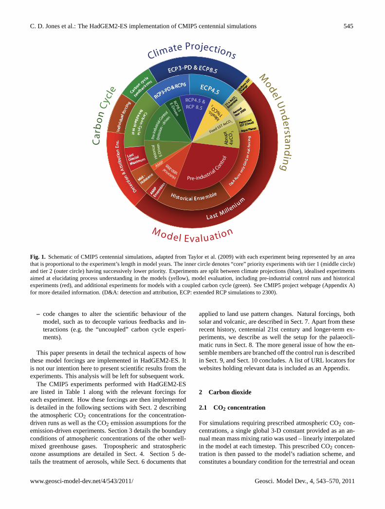
There are a number of new types of experiments proposedfor CMIP5 in comparison with previous incarnations. As inprevious intercomparison exercises, the main focus and effortrests on the longer time-scale (“centennial”) experiments,including now emission-driven runs of models that includea coupled carbon-cycle (ESMs). These centennial experi-ments are being performed at the Met Office Hadley Centrewith the HadGEM2-ES Earth System model (Collins et al.,2011; Martin et al., 2011); a configuration of the Met Of-fice’s Unified Model. Figure 1 outlines the main experimentsand groups them into categories. The inner circle denotes“core” priority experiments with tier 1 (middle circle) andtier 2 (outer circle) having successively lower priority. Ex-periments are split between climate projections (blue), ide-alised experiments aimed at elucidating process understand-ing in the models (yellow), model evaluation, including pre-industrial control runs and historical experiments (red), andadditional experiments for models with a coupled carbon cy-cle (green).
In the following, we briefly describe HadGEM2-ES ESM,which is documented in detail in Collins et al. (2011).HadGEM2-ES is a coupled AOGCM with atmospheric reso-lution of N96 (1.875◦ × 1.25◦) with 38 vertical levels and anocean resolution of 1◦ (increasing to 1/3◦ at the equator) and40 vertical levels. HadGEM2-ES also represents interactiveland and ocean carbon cycles and dynamic vegetation with anoption to prescribe either atmospheric CO2 concentrations orto prescribe anthropogenic CO2 emissions and simulate CO2concentrations as described in Sect. 2. An interactive tropo-spheric chemistry scheme is also included, which simulatesthe evolution of atmospheric composition and interactionswith atmospheric aerosols. The model timestep is 30 min(atmosphere and land) and 1 h (ocean). Extensive diagnos-tic output is being made available to the CMIP5 multi-modelarchive. Output is available either at certain prescribed fre-quencies or as time-average values over certain periods asdetailed in the CMIP5 output guidelines (see URL 2 in Ap-pendix A).
The CMIP5 simulations include 4 future scenarios re-ferred to as “Representative Concentration Pathways” orRCPs (Moss et al., 2010). These future scenarios havebeen generated by four integrated assessment models (IAMs)and selected from over 300 published scenarios of futuregreenhouse gas emissions resulting from socio-economicand energy-system modelling. These RCPs are labelled ac-cording to the approximate global radiative forcing level in2100 for RCP8.5 (Riahi et al., 2007), during stabilisation af-ter 2150 for RCP4.5 (Clarke et al., 2007; Smith and Wigley,2006) and RCP6 (Fujino et al., 2006) or the point of maxi-mal forcing levels in the case RCP3-PD (van Vuuren et al.,2006, 2007), with PD standing for “Peak and Decline”. Thelatter scenario has previously been known as RCP2.6, as ra-diative forcing levels decline towards 2.6 Wm−2 by 2100.Note that these radiative forcing levels are illustrative only,because greenhouse gas concentrations, aerosol and tropo-spheric ozone precursors are prescribed, resulting in a widespread in radiative forcings across different models.
The experimental protocol involves performing a histori-cal simulation (defined for HadGEM2-ES as 1860 to 2005)using the historical record of climate forcing factors such asgreenhouse gases, aerosols and natural forcings such as solarand volcanic changes. The model state at 2005 is then usedas the initial condition for the 4 future RCP simulations. Fur-ther extension of the RCP simulations to 2300 is also imple-mented as detailed in the RCP White Paper (see URL 3 inAppendix A) and Meinshausen et al. (2011).
Many of these experiments require technical implementa-tion by means of either or both of the following:
– time-varying boundary conditions such as concentra-tions of greenhouse gases or emissions of reactivechemical species or aerosol pre-cursors. These may begiven as single, global-mean numbers, or supplied as2-D or 3-D fields of data,
Geosci. Model Dev., 4, 543–570, 2011 www.geosci-model-dev.net/4/543/2011/
C. D. Jones et al.: The HadGEM2-ES implementation of CMIP5 centennial simulations 545
(c) Malte Meinshausen after K. E. Taylor (2009)
Uniform
SST
feedback te
st
Carb
on cycle
Dete
ctio
n &
Att
rib
uti
on
En
s.In
div
idu
al fo
rcin
g
Last Milleniu
m
ECP3-PD & ECP8.5
RCP3-PD & RCP6 ECP4.5
D&A Runs
onl
y G
HG
or
nat
. fo
rcin
g
feeed
ba
ck test
Carb
on
Cycle
AMIP
Ense
mble
s
Mid -
Holocene
Last
Glacial
Maximum
Historical Ense m ble
RCP4.5 &RCP8.5
E-Driven 1%
CO2
4xC
O2
Id
ealis.
Ab
rup
t
Pre-industrial C
ontrol
E-D
riven
Emis
sion
- dr
ive
n
AMIP
Pre-
indu
stria
l Con
trol
Fixed SST 4xCO 2
Historic
al
Hist
oric
al
1850-20
05
RCP 8.5
M odel Evaluation
Car
bo
n C
ycle
Climate Projections
Model U
nd
erstand
ing
Fig. 1. Schematic of CMIP5 centennial simulations, adapted from Taylor et al. (2009) with each experiment being represented by an areathat is proportional to the experiment’s length in model years. The inner circle denotes “core” priority experiments with tier 1 (middle circle)and tier 2 (outer circle) having successively lower priority. Experiments are split between climate projections (blue), idealised experimentsaimed at elucidating process understanding in the models (yellow), model evaluation, including pre-industrial control runs and historicalexperiments (red), and additional experiments for models with a coupled carbon cycle (green). See CMIP5 project webpage (Appendix A)for more detailed information. (D&A: detection and attribution, ECP: extended RCP simulations to 2300).
– code changes to alter the scientific behaviour of themodel, such as to decouple various feedbacks and in-teractions (e.g. the “uncoupled” carbon cycle experi-ments).
This paper presents in detail the technical aspects of howthese model forcings are implemented in HadGEM2-ES. Itis not our intention here to present scientific results from theexperiments. This analysis will be left for subsequent work.
The CMIP5 experiments performed with HadGEM2-ESare listed in Table 1 along with the relevant forcings foreach experiment. How these forcings are then implementedis detailed in the following sections with Sect. 2 describingthe atmospheric CO2 concentrations for the concentration-driven runs as well as the CO2 emission assumptions for theemission-driven experiments. Section 3 details the boundaryconditions of atmospheric concentrations of the other well-mixed greenhouse gases. Tropospheric and stratosphericozone assumptions are detailed in Sect. 4. Section 5 de-tails the treatment of aerosols, while Sect. 6 documents that
applied to land use pattern changes. Natural forcings, bothsolar and volcanic, are described in Sect. 7. Apart from theserecent history, centennial 21st century and longer-term ex-periments, we describe as well the setup for the palaeocli-matic runs in Sect. 8. The more general issue of how the en-semble members are branched off the control run is describedin Sect. 9, and Sect. 10 concludes. A list of URL locators forwebsites holding relevant data is included as an Appendix.
2 Carbon dioxide
2.1 CO2 concentration
For simulations requiring prescribed atmospheric CO2 con-centrations, a single global 3-D constant provided as an an-nual mean mass mixing ratio was used – linearly interpolatedin the model at each timestep. This prescribed CO2 concen-tration is then passed to the model’s radiation scheme, andconstitutes a boundary condition for the terrestrial and ocean
www.geosci-model-dev.net/4/543/2011/ Geosci. Model Dev., 4, 543–570, 2011
546 C. D. Jones et al.: The HadGEM2-ES implementation of CMIP5 centennial simulations
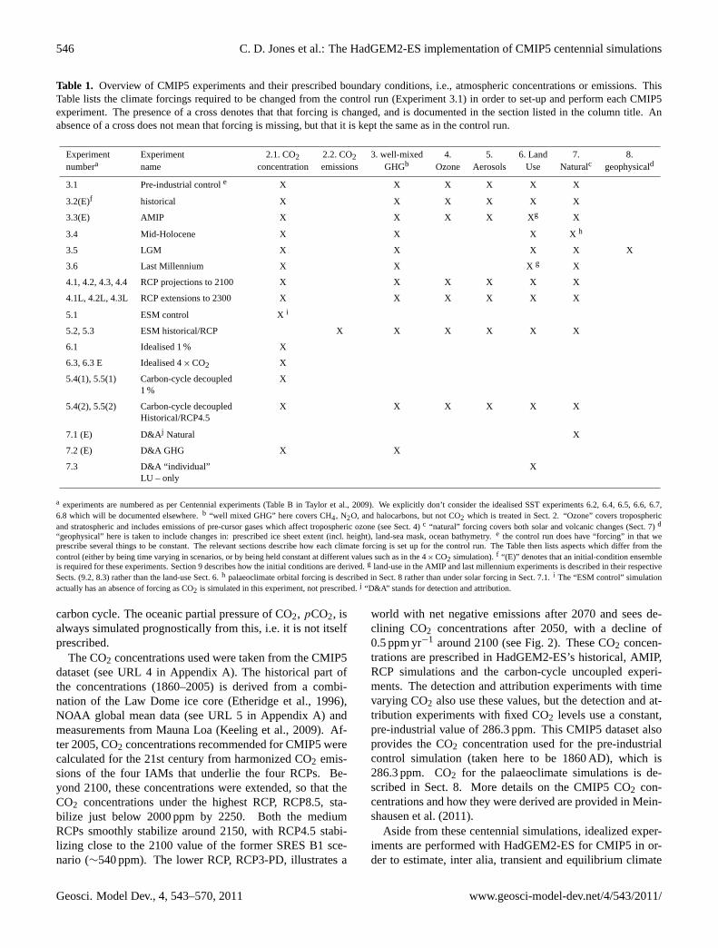
Table 1. Overview of CMIP5 experiments and their prescribed boundary conditions, i.e., atmospheric concentrations or emissions. ThisTable lists the climate forcings required to be changed from the control run (Experiment 3.1) in order to set-up and perform each CMIP5experiment. The presence of a cross denotes that that forcing is changed, and is documented in the section listed in the column title. Anabsence of a cross does not mean that forcing is missing, but that it is kept the same as in the control run.
Experiment Experiment 2.1. CO2 2.2. CO2 3. well-mixed 4. 5. 6. Land 7. 8.numbera name concentration emissions GHGb Ozone Aerosols Use Naturalc geophysicald
3.1 Pre-industrial controle X X X X X X
3.2(E)f historical X X X X X X
3.3(E) AMIP X X X X X g X
3.4 Mid-Holocene X X X Xh
3.5 LGM X X X X X
3.6 Last Millennium X X Xg X
4.1, 4.2, 4.3, 4.4 RCP projections to 2100 X X X X X X
4.1L, 4.2L, 4.3L RCP extensions to 2300 X X X X X X
5.1 ESM control Xi
5.2, 5.3 ESM historical/RCP X X X X X X
6.1 Idealised 1 % X
6.3, 6.3 E Idealised 4× CO2 X
5.4(1), 5.5(1) Carbon-cycle decoupled1 %
X
5.4(2), 5.5(2) Carbon-cycle decoupledHistorical/RCP4.5
X X X X X X
7.1 (E) D&Aj Natural X
7.2 (E) D&A GHG X X
7.3 D&A “individual”LU – only
X
a experiments are numbered as per Centennial experiments (Table B in Taylor et al., 2009). We explicitly don’t consider the idealised SST experiments 6.2, 6.4, 6.5, 6.6, 6.7,6.8 which will be documented elsewhere.b “well mixed GHG” here covers CH4, N2O, and halocarbons, but not CO2 which is treated in Sect. 2. “Ozone” covers troposphericand stratospheric and includes emissions of pre-cursor gases which affect tropospheric ozone (see Sect. 4)c “natural” forcing covers both solar and volcanic changes (Sect. 7)d
“geophysical” here is taken to include changes in: prescribed ice sheet extent (incl. height), land-sea mask, ocean bathymetry.e the control run does have “forcing” in that weprescribe several things to be constant. The relevant sections describe how each climate forcing is set up for the control run. The Table then lists aspects which differ from thecontrol (either by being time varying in scenarios, or by being held constant at different values such as in the 4× CO2 simulation).f “(E)” denotes that an initial-condition ensembleis required for these experiments. Section 9 describes how the initial conditions are derived.g land-use in the AMIP and last millennium experiments is described in their respectiveSects. (9.2, 8.3) rather than the land-use Sect. 6.h palaeoclimate orbital forcing is described in Sect. 8 rather than under solar forcing in Sect. 7.1.i The “ESM control” simulationactually has an absence of forcing as CO2 is simulated in this experiment, not prescribed.j “D&A” stands for detection and attribution.
carbon cycle. The oceanic partial pressure of CO2, pCO2, isalways simulated prognostically from this, i.e. it is not itselfprescribed.
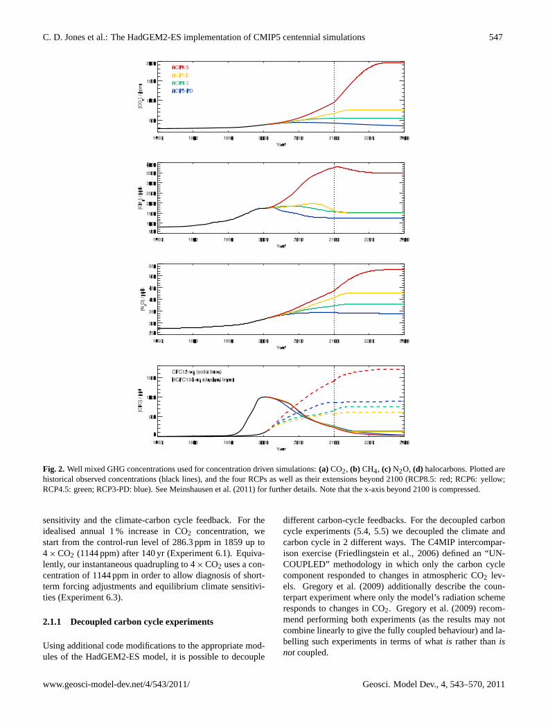
The CO2 concentrations used were taken from the CMIP5dataset (see URL 4 in Appendix A). The historical part ofthe concentrations (1860–2005) is derived from a combi-nation of the Law Dome ice core (Etheridge et al., 1996),NOAA global mean data (see URL 5 in Appendix A) andmeasurements from Mauna Loa (Keeling et al., 2009). Af-ter 2005, CO2 concentrations recommended for CMIP5 werecalculated for the 21st century from harmonized CO2 emis-sions of the four IAMs that underlie the four RCPs. Be-yond 2100, these concentrations were extended, so that theCO2 concentrations under the highest RCP, RCP8.5, sta-bilize just below 2000 ppm by 2250. Both the mediumRCPs smoothly stabilize around 2150, with RCP4.5 stabi-lizing close to the 2100 value of the former SRES B1 sce-nario (∼540 ppm). The lower RCP, RCP3-PD, illustrates a
world with net negative emissions after 2070 and sees de-clining CO2 concentrations after 2050, with a decline of0.5 ppm yr−1 around 2100 (see Fig. 2). These CO2 concen-trations are prescribed in HadGEM2-ES’s historical, AMIP,RCP simulations and the carbon-cycle uncoupled experi-ments. The detection and attribution experiments with timevarying CO2 also use these values, but the detection and at-tribution experiments with fixed CO2 levels use a constant,pre-industrial value of 286.3 ppm. This CMIP5 dataset alsoprovides the CO2 concentration used for the pre-industrialcontrol simulation (taken here to be 1860 AD), which is286.3 ppm. CO2 for the palaeoclimate simulations is de-scribed in Sect. 8. More details on the CMIP5 CO2 con-centrations and how they were derived are provided in Mein-shausen et al. (2011).
Aside from these centennial simulations, idealized exper-iments are performed with HadGEM2-ES for CMIP5 in or-der to estimate, inter alia, transient and equilibrium climate
Geosci. Model Dev., 4, 543–570, 2011 www.geosci-model-dev.net/4/543/2011/
C. D. Jones et al.: The HadGEM2-ES implementation of CMIP5 centennial simulations 547
Fig. 2. Well mixed GHG concentrations used for concentration driven simulations:(a) CO2, (b) CH4, (c) N2O, (d) halocarbons. Plotted arehistorical observed concentrations (black lines), and the four RCPs as well as their extensions beyond 2100 (RCP8.5: red; RCP6: yellow;RCP4.5: green; RCP3-PD: blue). See Meinshausen et al. (2011) for further details. Note that the x-axis beyond 2100 is compressed.
sensitivity and the climate-carbon cycle feedback. For theidealised annual 1 % increase in CO2 concentration, westart from the control-run level of 286.3 ppm in 1859 up to4× CO2 (1144 ppm) after 140 yr (Experiment 6.1). Equiva-lently, our instantaneous quadrupling to 4× CO2 uses a con-centration of 1144 ppm in order to allow diagnosis of short-term forcing adjustments and equilibrium climate sensitivi-ties (Experiment 6.3).
2.1.1 Decoupled carbon cycle experiments
Using additional code modifications to the appropriate mod-ules of the HadGEM2-ES model, it is possible to decouple
different carbon-cycle feedbacks. For the decoupled carboncycle experiments (5.4, 5.5) we decoupled the climate andcarbon cycle in 2 different ways. The C4MIP intercompar-ison exercise (Friedlingstein et al., 2006) defined an “UN-COUPLED” methodology in which only the carbon cyclecomponent responded to changes in atmospheric CO2 lev-els. Gregory et al. (2009) additionally describe the coun-terpart experiment where only the model’s radiation schemeresponds to changes in CO2. Gregory et al. (2009) recom-mend performing both experiments (as the results may notcombine linearly to give the fully coupled behaviour) and la-belling such experiments in terms of whatis rather thanisnotcoupled.
www.geosci-model-dev.net/4/543/2011/ Geosci. Model Dev., 4, 543–570, 2011
548 C. D. Jones et al.: The HadGEM2-ES implementation of CMIP5 centennial simulations
Hence we performed the biogeochemically coupled(“BGC”) experiments (5.4) in which the models biogeo-chemistry is coupled (i.e., the biogeochemistry modules re-spond to the changing atmospheric CO2 concentration) andthe radiation scheme is uncoupled (and uses the preindustriallevel of CO2 which is held constant) and also radiatively cou-pled (“RAD”) experiments (5.5) in which the model’s radia-tion scheme is allowed to respond to changes in atmosphericCO2 levels, but the biogeochemistry components (land veg-etation and ocean chemistry and ecosystem) use a constantCO2 level, again set to the preindustrial value. Both decou-pled experiments can be achieved with single simulations inwhich time-varying or time-fixed values of CO2 are used asinput data to the respective sections of model code. We per-formed both BGC and RAD experiments for the idealised(1 %) and transient, multi-forcing (historical/RCP4.5) sce-narios.
2.2 CO2 emissions
2.2.1 Emissions data
In addition to running with prescribed atmospheric CO2 con-centrations, HadGEM2-ES can be configured to run witha fully interactive carbon cycle. Here, atmospheric CO2is treated as a 3-D prognostic tracer, transported by atmo-spheric circulation, and free to evolve in response to pre-scribed surface emissions and simulated natural fluxes to andfrom the oceans and land. This approach is required forthe “Emission-driven” simulations (5.1–5.3) shown in greenin Fig. 1, and it also allows additional model evaluation bycomparison with flask and station measuring sites such as atMauna Loa (e.g. Law et al., 2006; Cadule et al., 2010).
A 2-D timeseries of total anthropogenic emissions wasconstructed by summing contributions from fossil fuel useand land-use change. For the historical simulation, annualmean emissions from fossil fuel burning, cement manufac-ture, and gas-flaring were provided on a 1◦
× 1◦ grid from1850 to 1949 (Boden et al., 2010), with monthly means from1950 to 2005 (Andres et al., 2011). For the RCP8.5 simula-tion, the harmonized fossil fuel emissions for 2005 to 2100were used (as available in the RCP database, see URL 6in Appendix A). The land use change (LUC) emissions arebased on the regional totals of Houghton (2008), which wereprovided as annual means of the period 1850–2005. Withineach of the ten regions the emissions were linearly weightedby population density on a 1◦
× 1◦ grid (for more informa-tion, see URL 7 in Appendix A). These population data werealso used by Klein Goldewijk (2001) and are linearly interpo-lated between the years 1850, 1900, 1910, 1920, 1930, 1940,1950, 1960, 1970, 1980, and 1990. After the year 1990 popu-lation density is assumed to stay constant. Additionally, highpopulation density was set to a limit of 20 persons per km2 toavoid large emissions in urban centres. The weighting withpopulation data inhibits land use change emissions in deserts
and high northern latitudes, which improves the latitudinaldistribution of the emissions. However, the method is insuf-ficient to provide realistic local land use change emissions(e.g. in tropical forests).
The gridded (1◦ × 1◦) fossil fuel and land-use emissionsdata, originally provided as a flux per gridbox, were con-verted to flux per unit area, then regridded as annual meansonto the HadGEM2-ES model grid. A small scaling adjust-ment was made after regridding to ensure the global totalsmatched those of the 1◦
× 1◦ data exactly. Future emissionswere not provided with spatial information so we scaled the2005 geographical pattern for fossil-fuel and land-use emis-sions to give the correct global total into the future. TheCO2 emissions are updated daily in the model by linearlyinterpolation between the annual values (or monthly, from1950–2005). HadGEM2-ES has the functionality to inter-actively simulate land-use emissions of CO2 directly from aprescribed scenario of land-use change and simulated vegeta-tion cover and biomass (see Sect. 6). However, the model hasnot been fully evaluated in this respect, so for CMIP5 exper-iments we disable this feature and choose rather to prescribereconstructed land-use emissions from Houghton (2008). Bysimulating changes in carbon storage due to imposed landuse change, but imposing land-use CO2 emissions to the at-mosphere from an external dataset we introduce some degreeof inconsistency in this simulation. Work is required to eval-uate and improve the simulation of land-use emissions so thatthey can be used interactively in such simulations in the fu-ture.
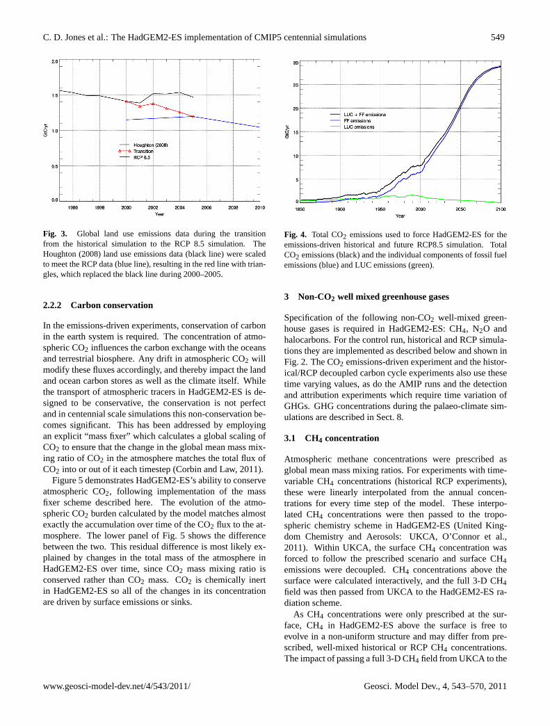
The uncertainty in annual land-use emissions of±0.5 GtC(cf. Le Quere et al., 2009) is relatively large comparedto the total land use emissions (an estimated 1.467 GtC in2005, Houghton, 2008). The RCP scenarios have beenharmonised towards the average LUC emission value ofall four original IAM emission estimates, i.e., 1.196 GtCin 2005. This is substantially lower than the value calcu-lated by Houghton (2008) of 1.467 GtC in the same year,although still within the uncertainty. The climate-carboncycle modelling community preferred to use the originalHoughton (2008) estimates for historical emissions. Asmooth transition between the historical and the RCP simula-tions was ensured by scaling the last five years of the histori-cal LUC emissions to factor in a linearly-increasing contribu-tion from the harmonised RCP values. In 2001 the two val-ues were combined in the ratio 80 %:20 % (Houghton: RCP),followed by 60 %:40 % in 2002, and so on until 0 %:100 %(i.e. the RCP value) in 2005, as shown in Fig. 3.
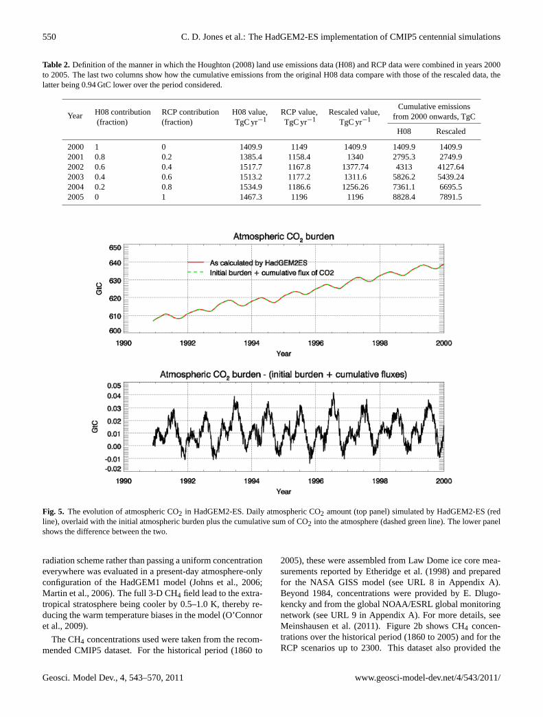
By rescaling the Houghton (2008) data between 2000 and2005 to merge smoothly with the RCP value in 2005, welower total emissions in this period by 0.94 GtC compared tothe original Houghton estimates (Table 2). In the presence offossil emissions of more than 40 GtC in this period this dif-ference is small. Total emissions and the relative contributionof fossil fuel and LUC are shown in Fig. 4.
Geosci. Model Dev., 4, 543–570, 2011 www.geosci-model-dev.net/4/543/2011/
C. D. Jones et al.: The HadGEM2-ES implementation of CMIP5 centennial simulations 549
Fig. 3. Global land use emissions data during the transitionfrom the historical simulation to the RCP 8.5 simulation. TheHoughton (2008) land use emissions data (black line) were scaledto meet the RCP data (blue line), resulting in the red line with trian-gles, which replaced the black line during 2000–2005.
2.2.2 Carbon conservation
In the emissions-driven experiments, conservation of carbonin the earth system is required. The concentration of atmo-spheric CO2 influences the carbon exchange with the oceansand terrestrial biosphere. Any drift in atmospheric CO2 willmodify these fluxes accordingly, and thereby impact the landand ocean carbon stores as well as the climate itself. Whilethe transport of atmospheric tracers in HadGEM2-ES is de-signed to be conservative, the conservation is not perfectand in centennial scale simulations this non-conservation be-comes significant. This has been addressed by employingan explicit “mass fixer” which calculates a global scaling ofCO2 to ensure that the change in the global mean mass mix-ing ratio of CO2 in the atmosphere matches the total flux ofCO2 into or out of it each timestep (Corbin and Law, 2011).
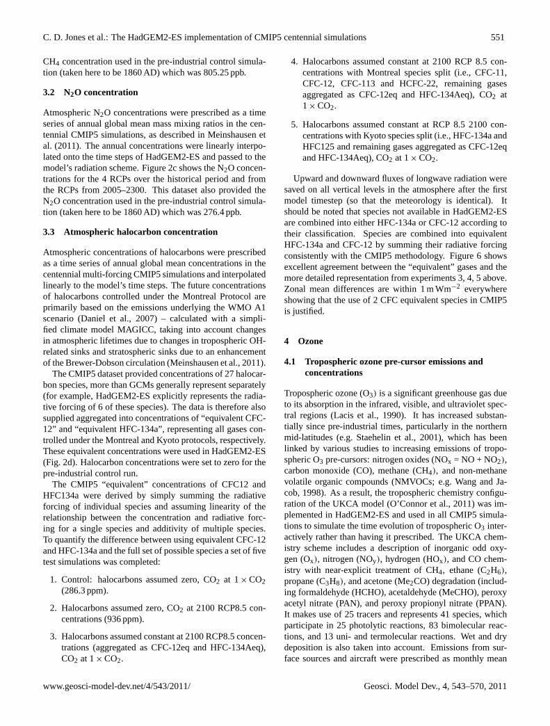
Figure 5 demonstrates HadGEM2-ES’s ability to conserveatmospheric CO2, following implementation of the massfixer scheme described here. The evolution of the atmo-spheric CO2 burden calculated by the model matches almostexactly the accumulation over time of the CO2 flux to the at-mosphere. The lower panel of Fig. 5 shows the differencebetween the two. This residual difference is most likely ex-plained by changes in the total mass of the atmosphere inHadGEM2-ES over time, since CO2 mass mixing ratio isconserved rather than CO2 mass. CO2 is chemically inertin HadGEM2-ES so all of the changes in its concentrationare driven by surface emissions or sinks.
Fig. 4. Total CO2 emissions used to force HadGEM2-ES for theemissions-driven historical and future RCP8.5 simulation. TotalCO2 emissions (black) and the individual components of fossil fuelemissions (blue) and LUC emissions (green).
3 Non-CO2 well mixed greenhouse gases
Specification of the following non-CO2 well-mixed green-house gases is required in HadGEM2-ES: CH4, N2O andhalocarbons. For the control run, historical and RCP simula-tions they are implemented as described below and shown inFig. 2. The CO2 emissions-driven experiment and the histor-ical/RCP decoupled carbon cycle experiments also use thesetime varying values, as do the AMIP runs and the detectionand attribution experiments which require time variation ofGHGs. GHG concentrations during the palaeo-climate sim-ulations are described in Sect. 8.
3.1 CH4 concentration
Atmospheric methane concentrations were prescribed asglobal mean mass mixing ratios. For experiments with time-variable CH4 concentrations (historical RCP experiments),these were linearly interpolated from the annual concen-trations for every time step of the model. These interpo-lated CH4 concentrations were then passed to the tropo-spheric chemistry scheme in HadGEM2-ES (United King-dom Chemistry and Aerosols: UKCA, O’Connor et al.,2011). Within UKCA, the surface CH4 concentration wasforced to follow the prescribed scenario and surface CH4emissions were decoupled. CH4 concentrations above thesurface were calculated interactively, and the full 3-D CH4field was then passed from UKCA to the HadGEM2-ES ra-diation scheme.
As CH4 concentrations were only prescribed at the sur-face, CH4 in HadGEM2-ES above the surface is free toevolve in a non-uniform structure and may differ from pre-scribed, well-mixed historical or RCP CH4 concentrations.The impact of passing a full 3-D CH4 field from UKCA to the
www.geosci-model-dev.net/4/543/2011/ Geosci. Model Dev., 4, 543–570, 2011
550 C. D. Jones et al.: The HadGEM2-ES implementation of CMIP5 centennial simulations
Table 2. Definition of the manner in which the Houghton (2008) land use emissions data (H08) and RCP data were combined in years 2000to 2005. The last two columns show how the cumulative emissions from the original H08 data compare with those of the rescaled data, thelatter being 0.94 GtC lower over the period considered.
Year H08 contribution RCP contribution H08 value, RCP value, Rescaled value,Cumulative emissions
(fraction) (fraction) TgC yr−1 TgC yr−1 TgC yr−1 from 2000 onwards, TgC
H08 Rescaled
2000 1 0 1409.9 1149 1409.9 1409.9 1409.92001 0.8 0.2 1385.4 1158.4 1340 2795.3 2749.92002 0.6 0.4 1517.7 1167.8 1377.74 4313 4127.642003 0.4 0.6 1513.2 1177.2 1311.6 5826.2 5439.242004 0.2 0.8 1534.9 1186.6 1256.26 7361.1 6695.52005 0 1 1467.3 1196 1196 8828.4 7891.5
Fig. 5. The evolution of atmospheric CO2 in HadGEM2-ES. Daily atmospheric CO2 amount (top panel) simulated by HadGEM2-ES (redline), overlaid with the initial atmospheric burden plus the cumulative sum of CO2 into the atmosphere (dashed green line). The lower panelshows the difference between the two.
radiation scheme rather than passing a uniform concentrationeverywhere was evaluated in a present-day atmosphere-onlyconfiguration of the HadGEM1 model (Johns et al., 2006;Martin et al., 2006). The full 3-D CH4 field lead to the extra-tropical stratosphere being cooler by 0.5–1.0 K, thereby re-ducing the warm temperature biases in the model (O’Connoret al., 2009).
The CH4 concentrations used were taken from the recom-mended CMIP5 dataset. For the historical period (1860 to
2005), these were assembled from Law Dome ice core mea-surements reported by Etheridge et al. (1998) and preparedfor the NASA GISS model (see URL 8 in Appendix A).Beyond 1984, concentrations were provided by E. Dlugo-kencky and from the global NOAA/ESRL global monitoringnetwork (see URL 9 in Appendix A). For more details, seeMeinshausen et al. (2011). Figure 2b shows CH4 concen-trations over the historical period (1860 to 2005) and for theRCP scenarios up to 2300. This dataset also provided the
Geosci. Model Dev., 4, 543–570, 2011 www.geosci-model-dev.net/4/543/2011/
C. D. Jones et al.: The HadGEM2-ES implementation of CMIP5 centennial simulations 551
CH4 concentration used in the pre-industrial control simula-tion (taken here to be 1860 AD) which was 805.25 ppb.
3.2 N2O concentration
Atmospheric N2O concentrations were prescribed as a timeseries of annual global mean mass mixing ratios in the cen-tennial CMIP5 simulations, as described in Meinshausen etal. (2011). The annual concentrations were linearly interpo-lated onto the time steps of HadGEM2-ES and passed to themodel’s radiation scheme. Figure 2c shows the N2O concen-trations for the 4 RCPs over the historical period and fromthe RCPs from 2005–2300. This dataset also provided theN2O concentration used in the pre-industrial control simula-tion (taken here to be 1860 AD) which was 276.4 ppb.
3.3 Atmospheric halocarbon concentration
Atmospheric concentrations of halocarbons were prescribedas a time series of annual global mean concentrations in thecentennial multi-forcing CMIP5 simulations and interpolatedlinearly to the model’s time steps. The future concentrationsof halocarbons controlled under the Montreal Protocol areprimarily based on the emissions underlying the WMO A1scenario (Daniel et al., 2007) – calculated with a simpli-fied climate model MAGICC, taking into account changesin atmospheric lifetimes due to changes in tropospheric OH-related sinks and stratospheric sinks due to an enhancementof the Brewer-Dobson circulation (Meinshausen et al., 2011).
The CMIP5 dataset provided concentrations of 27 halocar-bon species, more than GCMs generally represent separately(for example, HadGEM2-ES explicitly represents the radia-tive forcing of 6 of these species). The data is therefore alsosupplied aggregated into concentrations of “equivalent CFC-12” and “equivalent HFC-134a”, representing all gases con-trolled under the Montreal and Kyoto protocols, respectively.These equivalent concentrations were used in HadGEM2-ES(Fig. 2d). Halocarbon concentrations were set to zero for thepre-industrial control run.
The CMIP5 “equivalent” concentrations of CFC12 andHFC134a were derived by simply summing the radiativeforcing of individual species and assuming linearity of therelationship between the concentration and radiative forc-ing for a single species and additivity of multiple species.To quantify the difference between using equivalent CFC-12and HFC-134a and the full set of possible species a set of fivetest simulations was completed:
1. Control: halocarbons assumed zero, CO2 at 1× CO2(286.3 ppm).
2. Halocarbons assumed zero, CO2 at 2100 RCP8.5 con-centrations (936 ppm).
3. Halocarbons assumed constant at 2100 RCP8.5 concen-trations (aggregated as CFC-12eq and HFC-134Aeq),CO2 at 1× CO2.
4. Halocarbons assumed constant at 2100 RCP 8.5 con-centrations with Montreal species split (i.e., CFC-11,CFC-12, CFC-113 and HCFC-22, remaining gasesaggregated as CFC-12eq and HFC-134Aeq), CO2 at1× CO2.
5. Halocarbons assumed constant at RCP 8.5 2100 con-centrations with Kyoto species split (i.e., HFC-134a andHFC125 and remaining gases aggregated as CFC-12eqand HFC-134Aeq), CO2 at 1× CO2.
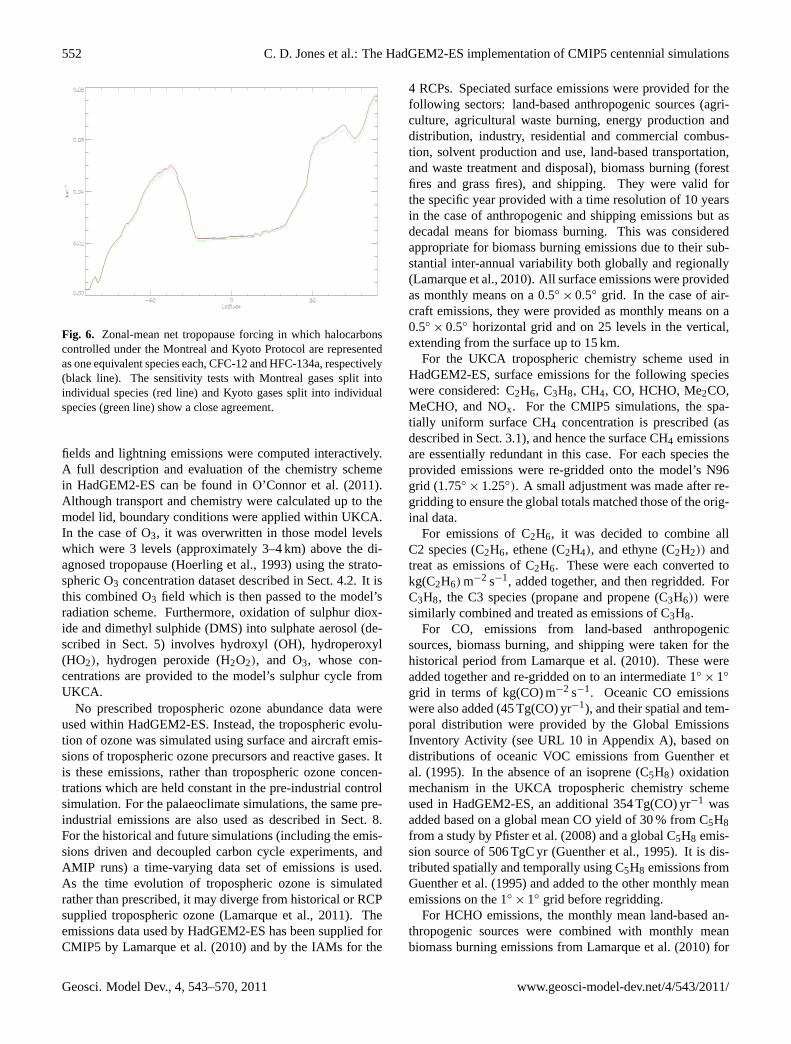
Upward and downward fluxes of longwave radiation weresaved on all vertical levels in the atmosphere after the firstmodel timestep (so that the meteorology is identical). Itshould be noted that species not available in HadGEM2-ESare combined into either HFC-134a or CFC-12 according totheir classification. Species are combined into equivalentHFC-134a and CFC-12 by summing their radiative forcingconsistently with the CMIP5 methodology. Figure 6 showsexcellent agreement between the “equivalent” gases and themore detailed representation from experiments 3, 4, 5 above.Zonal mean differences are within 1 m Wm−2 everywhereshowing that the use of 2 CFC equivalent species in CMIP5is justified.
4 Ozone
4.1 Tropospheric ozone pre-cursor emissions andconcentrations
Tropospheric ozone (O3) is a significant greenhouse gas dueto its absorption in the infrared, visible, and ultraviolet spec-tral regions (Lacis et al., 1990). It has increased substan-tially since pre-industrial times, particularly in the northernmid-latitudes (e.g. Staehelin et al., 2001), which has beenlinked by various studies to increasing emissions of tropo-spheric O3 pre-cursors: nitrogen oxides (NOx = NO + NO2),carbon monoxide (CO), methane (CH4), and non-methanevolatile organic compounds (NMVOCs; e.g. Wang and Ja-cob, 1998). As a result, the tropospheric chemistry configu-ration of the UKCA model (O’Connor et al., 2011) was im-plemented in HadGEM2-ES and used in all CMIP5 simula-tions to simulate the time evolution of tropospheric O3 inter-actively rather than having it prescribed. The UKCA chem-istry scheme includes a description of inorganic odd oxy-gen (Ox), nitrogen (NOy), hydrogen (HOx), and CO chem-istry with near-explicit treatment of CH4, ethane (C2H6),propane (C3H8), and acetone (Me2CO) degradation (includ-ing formaldehyde (HCHO), acetaldehyde (MeCHO), peroxyacetyl nitrate (PAN), and peroxy propionyl nitrate (PPAN).It makes use of 25 tracers and represents 41 species, whichparticipate in 25 photolytic reactions, 83 bimolecular reac-tions, and 13 uni- and termolecular reactions. Wet and drydeposition is also taken into account. Emissions from sur-face sources and aircraft were prescribed as monthly mean
www.geosci-model-dev.net/4/543/2011/ Geosci. Model Dev., 4, 543–570, 2011
552 C. D. Jones et al.: The HadGEM2-ES implementation of CMIP5 centennial simulations
Fig. 6. Zonal-mean net tropopause forcing in which halocarbonscontrolled under the Montreal and Kyoto Protocol are representedas one equivalent species each, CFC-12 and HFC-134a, respectively(black line). The sensitivity tests with Montreal gases split intoindividual species (red line) and Kyoto gases split into individualspecies (green line) show a close agreement.
fields and lightning emissions were computed interactively.A full description and evaluation of the chemistry schemein HadGEM2-ES can be found in O’Connor et al. (2011).Although transport and chemistry were calculated up to themodel lid, boundary conditions were applied within UKCA.In the case of O3, it was overwritten in those model levelswhich were 3 levels (approximately 3–4 km) above the di-agnosed tropopause (Hoerling et al., 1993) using the strato-spheric O3 concentration dataset described in Sect. 4.2. It isthis combined O3 field which is then passed to the model’sradiation scheme. Furthermore, oxidation of sulphur diox-ide and dimethyl sulphide (DMS) into sulphate aerosol (de-scribed in Sect. 5) involves hydroxyl (OH), hydroperoxyl(HO2), hydrogen peroxide (H2O2), and O3, whose con-centrations are provided to the model’s sulphur cycle fromUKCA.
No prescribed tropospheric ozone abundance data wereused within HadGEM2-ES. Instead, the tropospheric evolu-tion of ozone was simulated using surface and aircraft emis-sions of tropospheric ozone precursors and reactive gases. Itis these emissions, rather than tropospheric ozone concen-trations which are held constant in the pre-industrial controlsimulation. For the palaeoclimate simulations, the same pre-industrial emissions are also used as described in Sect. 8.For the historical and future simulations (including the emis-sions driven and decoupled carbon cycle experiments, andAMIP runs) a time-varying data set of emissions is used.As the time evolution of tropospheric ozone is simulatedrather than prescribed, it may diverge from historical or RCPsupplied tropospheric ozone (Lamarque et al., 2011). Theemissions data used by HadGEM2-ES has been supplied forCMIP5 by Lamarque et al. (2010) and by the IAMs for the
4 RCPs. Speciated surface emissions were provided for thefollowing sectors: land-based anthropogenic sources (agri-culture, agricultural waste burning, energy production anddistribution, industry, residential and commercial combus-tion, solvent production and use, land-based transportation,and waste treatment and disposal), biomass burning (forestfires and grass fires), and shipping. They were valid forthe specific year provided with a time resolution of 10 yearsin the case of anthropogenic and shipping emissions but asdecadal means for biomass burning. This was consideredappropriate for biomass burning emissions due to their sub-stantial inter-annual variability both globally and regionally(Lamarque et al., 2010). All surface emissions were providedas monthly means on a 0.5◦
× 0.5◦ grid. In the case of air-craft emissions, they were provided as monthly means on a0.5◦
× 0.5◦ horizontal grid and on 25 levels in the vertical,extending from the surface up to 15 km.
For the UKCA tropospheric chemistry scheme used inHadGEM2-ES, surface emissions for the following specieswere considered: C2H6, C3H8, CH4, CO, HCHO, Me2CO,MeCHO, and NOx. For the CMIP5 simulations, the spa-tially uniform surface CH4 concentration is prescribed (asdescribed in Sect. 3.1), and hence the surface CH4 emissionsare essentially redundant in this case. For each species theprovided emissions were re-gridded onto the model’s N96grid (1.75◦ × 1.25◦). A small adjustment was made after re-gridding to ensure the global totals matched those of the orig-inal data.
For emissions of C2H6, it was decided to combine allC2 species (C2H6, ethene (C2H4), and ethyne (C2H2)) andtreat as emissions of C2H6. These were each converted tokg(C2H6) m−2 s−1, added together, and then regridded. ForC3H8, the C3 species (propane and propene (C3H6)) weresimilarly combined and treated as emissions of C3H8.
For CO, emissions from land-based anthropogenicsources, biomass burning, and shipping were taken for thehistorical period from Lamarque et al. (2010). These wereadded together and re-gridded on to an intermediate 1◦
× 1◦
grid in terms of kg(CO) m−2 s−1. Oceanic CO emissionswere also added (45 Tg(CO) yr−1), and their spatial and tem-poral distribution were provided by the Global EmissionsInventory Activity (see URL 10 in Appendix A), based ondistributions of oceanic VOC emissions from Guenther etal. (1995). In the absence of an isoprene (C5H8) oxidationmechanism in the UKCA tropospheric chemistry schemeused in HadGEM2-ES, an additional 354 Tg(CO) yr−1 wasadded based on a global mean CO yield of 30 % from C5H8from a study by Pfister et al. (2008) and a global C5H8 emis-sion source of 506 TgC yr (Guenther et al., 1995). It is dis-tributed spatially and temporally using C5H8 emissions fromGuenther et al. (1995) and added to the other monthly meanemissions on the 1◦ × 1◦ grid before regridding.
For HCHO emissions, the monthly mean land-based an-thropogenic sources were combined with monthly meanbiomass burning emissions from Lamarque et al. (2010) for
Geosci. Model Dev., 4, 543–570, 2011 www.geosci-model-dev.net/4/543/2011/
C. D. Jones et al.: The HadGEM2-ES implementation of CMIP5 centennial simulations 553
the historical period and re-gridded. Similar processing wasapplied to the future emissions supplied by the IAMs for the4 RCPs.
For MeCHO, the monthly mean NMVOC biomass burn-ing emissions from Lamarque et al. (2010) for the his-torical period were used. Using different emission fac-tors from Andreae and Merlet (2001) for grass fires, tropi-cal forest fires, and extra-tropical forest fires, emissions ofNMVOCs were converted into emissions of MeCHO (i.e.kg(MeCHO) m−2 s−1). Surface emissions of Me2CO weretaken from land-based anthropogenic sources and biomassburning from Lamarque et al. (2010, 2011). These wereadded together and re-gridded on to an intermediate 1◦
× 1◦
grid in terms of kg(Me2CO) m−2 s−1. Then, the dominantsource of Me2CO from vegetation was added, based on aglobal distribution from Guenther et al. (1995) and scaled togive a global annual total of 40.0 Tg(Me2CO) yr−1. The to-tal monthly mean emissions were then re-gridded on to themodel’s N96 grid. For future emissions, the processing wasidentical.
Finally for NOx surface emissions, contributions fromland-based anthropogenic sources, biomass burning, andshipping from Lamarque et al. (2010) were added togetherand re-gridded on to an intermediate 1◦
× 1◦ grid in termsof kg(NO) m−2 s−1. Added to these were a contribu-tion from natural soil emissions, based on a global andmonthly distribution provided by GEIA on a 1◦
× 1◦ grid(see URL 10 in Appendix A), and based on the global em-pirical model of soil-biogenic emissions from Yienger andLevy II (1995). These were scaled to contribute an additional12 Tg(NO) yr−1. A similar approach was adopted when pro-cessing the future emissions. All emissions provided wereprocessed as above for the years supplied and a linear inter-polation applied between years to produce emissions for ev-ery year. Figure 7 shows the time evolution of troposphericO3 pre-cursor surface emissions over the 1850–2100 timeperiod. After 2100, tropospheric ozone precursor emissionswere kept constant.
In the case of NOx emissions, 3-D emissions from aircraftwere also considered. These were supplied as monthly meanfields of either NO or NO2 on a 25 level (L25) 0.5× 0.5grid by Lamarque et al. (2010) for the historical period. ForHadGEM2-ES we used the NO emissions. They were firstre-gridded on to an N96× L25 grid and then projected onto the model’s N96× L38 grid, ensuring that the global an-nual total emissions were conserved. A similar approach wasadopted when processing the future emissions.
No additional coding in the HadGEM2-ES or UKCA mod-els was necessary for the treatment of tropospheric ozonepre-cursor emissions. The only code change was requiredfor the Detection and Attribution “greenhouse gases only”simulation (7.2). In this case, the UKCA model was modi-fied to maintain the global mean surface CH4 concentrationat pre-industrial levels i.e. 805.25 ppb. This was to ensurethat the increase in CH4 concentration as seen by the radi-
ation scheme did not affect concentrations of troposphericoxidants, thereby influencing the rate of sulphate aerosol for-mation.
4.2 Stratospheric ozone concentration
HadGEM2-ES requires stratospheric ozone to be input asmonthly zonal/height ancillary files. CMIP5 recommendsthe use of the AC&C/SPARC ozone database (Cionni et al.,2011) which covers the period 1850 to 2100 and can be usedin climate models that do not include interactive chemistry.The pre-industrial dataset consists of a repeating seasonal cy-cle of ozone values, and this is also used for the palaeocli-mate simulations described in Sect. 8. For the historical andfuture simulations (including the emissions driven and de-coupled carbon cycle experiments, and AMIP runs) a time-varying data set of stratospheric ozone is used.
The historical part of the AC&C/SPARC ozone databasespans the period 1850 to 2009 and consists of separate strato-spheric and tropospheric data sources. The future part ofthe AC&C/SPARC ozone database covers the period 2010 to2100 and seamlessly extends the historical database also in-cluding separate stratospheric and tropospheric data sourcesbased on 13 CCMs that performed a future simulation until2100 under the SRES A1B GHG scenario.
The AC&C/SPARC ozone is provided on pressure levelsbetween 1000-1 hPa. The UK National Centre for Atmo-spheric Science (NCAS) has produced an updated versionof the SPARC ozone dataset as follows.
A multiple-linear regression was performed on the his-torical raw pressure-level data between 1000-1 hPa consis-tent with the Randel and Wu (1999) method used to con-struct the timeseries. The ozone was then represented as:O3(t) = a∗SOL +b∗EESC + seasonalcycle + residuals. Forconsistency, the indices of 11-yr solar cycle (SOL) and totalequivalent chlorine (EESC) are identical to those used to pre-pare the original dataset. The SOL index is a 180.5 nm time-series provided by Fei Wu at NCAR. The standard SPARCozone dataset which extends into the future does not includesolar cycle variability post-2009. For production of a datasetextending into the future including an 11-yr ozone solar cy-cle, the solar regression index is used to build a future timeseries consistent with a repeating solar irradiance compiledby the Met Office Hadley Centre (see Sect. 7.1) and is mod-elled as a sinusoid with a period of 11 yr, with mean andmax-min values corresponding to solar cycle 23 normalisedagainst the 180.5 nm timeseries used in the historical ozone.There is no solar ozone signal in the high latitudes.
The data were then horizontally interpolated onto a N96grid. Vertical interpolation was achieved by hydrostati-cally mapping the SPARC ozone data from pressure surfacesonto pressure surface equivalent levels corresponding to theheight-based grid used by HadGEM2-ES using a scale heightof 7 km.
www.geosci-model-dev.net/4/543/2011/ Geosci. Model Dev., 4, 543–570, 2011

554 C. D. Jones et al.: The HadGEM2-ES implementation of CMIP5 centennial simulations
Fig. 7. Tropospheric ozone pre-cursor surface emissions over the historical period (1850–2005) and over the future period (2005–2100) fromthe 4 RCPs: RCP3-PD (blue), RCP4.5 (green), RCP6 (yellow), and RCP8.5 (red). The methane (CH4) emissions shown do not include acontribution from wetlands.
5 Tropospheric aerosol forcing
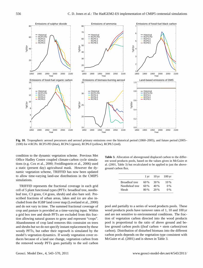
HadGEM2-ES simulates concentrations of six troposphericaerosol species: ammonium sulphate, fossil-fuel black car-bon, fossil-fuel organic carbon, biomass-burning, sea-salt,and mineral dust aerosols (Bellouin et al., 2007; Collins etal., 2011). Although an ammonium nitrate aerosol schemeis available to HadGEM2-ES, it was still in its developmen-tal version when CMIP5 simulations started, hence nitrateaerosols are not included in the CMIP5 simulations. In addi-tion, secondary organic aerosols from biogenic emissions arerepresented by a fixed climatology. All aerosol species canexert a direct effect by scattering and absorbing shortwaveand longwave radiation, and a semi-direct effect whereby thisdirect effect modifies atmospheric vertical profiles of tem-perature and clouds. In HadGEM2-ES all aerosol species,except fossil-fuel black carbon and mineral dust, also con-tribute to both the first and second indirect effects on clouds,modifying cloud albedo and precipitation efficiency, respec-tively. Changes in direct and indirect effects since 1860are termed aerosol radiative forcing. The magnitude of this
forcing depends on changes in aerosols, which are due in partto changes in emissions of primary aerosols and aerosol pre-cursors. Changes in emission rates are either derived fromexternal datasets or due to changes in the simulated climate.Here we document how any changes in emission rates areimplemented in the HadGEM2-ES CMIP5 centennial exper-iments. In the control run we specify a repeating seasonalcycle of 1860 emissions, and this is also used in the palaeocli-mate simulations (Sect. 8). Historical and future simulations(including the emissions-driven and decoupled carbon cycleexperiments and AMIP runs) use time-varying emissions asdescribed in this section.
In HadGEM2-ES sea-salt and mineral dust aerosol emis-sions are computed interactively, whereas emission datasetsdrive schemes for sulphate, fossil-fuel black and organic car-bon, and biomass aerosols. Unless otherwise stated, datasetsare derived from the historical and RCP time series preparedfor CMIP5. All non-interactive emission fields are interpo-lated by the model every five simulated days from prescribedmonthly-mean fields. Timeseries of non-interactive emis-sions are shown in Fig. 10. Aircraft emissions of aerosol
Geosci. Model Dev., 4, 543–570, 2011 www.geosci-model-dev.net/4/543/2011/
C. D. Jones et al.: The HadGEM2-ES implementation of CMIP5 centennial simulations 555
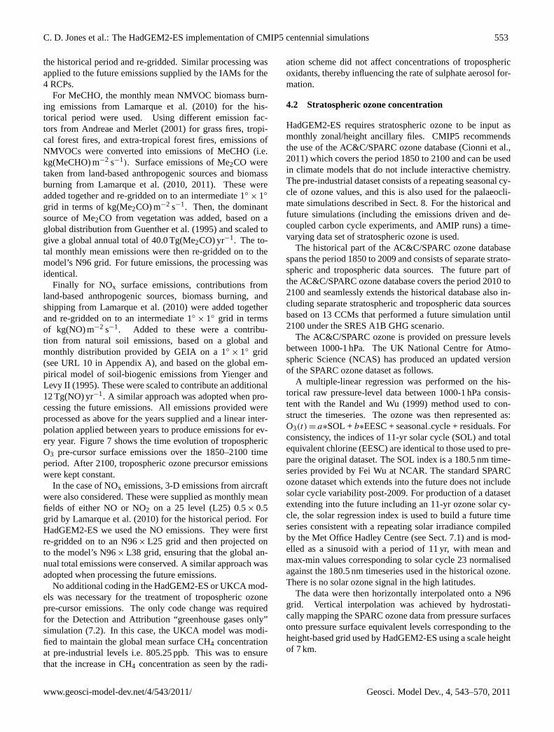
Fig. 8. Annual mean climatology of ozone volume mixing ration(ppmv) for 1979–2003.
precursors and primary aerosols are not included in themodel.
The sulphur cycle, which provides concentrations ofammonium sulphate aerosols, requires emissions of sul-phur dioxide (SO2) and dimethyl-sulphide (DMS). Sulphurdioxide emissions are derived from sector-based emissions.Emissions for all sectors are injected at the surface, exceptfor energy emissions and half of industrial emissions whichare injected at 0.5 km to represent chimney-level emissions.Sulphur dioxide emissions from biomass burning are not in-cluded. The model accounts for three-dimensional back-ground emissions of sulphur dioxide from degassing volca-noes, taken from Andres and Kasgnoc (1998). This rep-resents a constant rate of 0.62 Tg[S] yr−1 on a global av-erage, independent of the year simulated and is not partof the implementation of volcanic climate forcing whichwe discuss in Sect. 7.2. Similarly, land-based DMS emis-sions do not vary in time and give 0.86 Tg yr−1 (Spiro etal., 1992). Oceanic DMS emissions are provided interac-tively by the biogeochemical scheme of the ocean model as afunction of local chlorophyll concentrations and mixed layerdepth (based on Simo and Dachs, 2002). In an objectiveassessment against ship-board and time-series DMS obser-vations, the HadGEM2-ES interactive ocean DMS schemeperforms with similar skill to that found in the widely usedKettle et al. (1999) climatology (Halloran et al., 2010).The primary differences between the model-simulated andthe climatology-interpolated surface ocean DMS fields are;lower model Southern Hemisphere summer Southern OceanDMS concentrations, higher model annual equatorial DMSconcentrations, and a reduced model seasonal cycle ampli-tude. Oxidation of sulphur-dioxide and DMS into sulphateaerosol involves hydroxyl (OH), hydroperoxyl (HO2), hy-drogen peroxide (H2O2), and ozone (O3): concentrations forthose oxidants are provided by the tropospheric chemistryscheme.
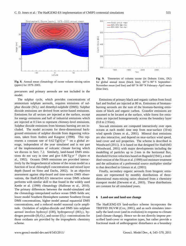
Fig. 9. Timeseries of column ozone (in Dobson Units, DU)for global annual mean (black line), 60◦ S–90◦ S September–November mean (red line) and 60◦ N–90◦ N February–April mean(blue line).
Emissions of primary black and organic carbon from fossilfuel and biofuel are injected at 80 m. Emissions of biomass-burning aerosols are the sum of the biomass-burning emis-sions of black and organic carbon. Grassfire emissions areassumed to be located at the surface, while forest fire emis-sions are injected homogeneously across the boundary layer(0.8 to 2.9 km).
Sea-salt emissions are computed interactively over openoceans at each model time step from near-surface (10 m)wind speeds (Jones et al., 2001). Mineral dust emissionsare also interactive, and depend on near-surface wind speed,land cover and soil properties. The scheme is described inWoodward (2011). It is based on that designed for HadAM3(Woodward, 2001) with major developments including themodelling of particles up to 2 mm in the horizontal flux,threshold friction velocities based on Bagnold (1941), a mod-ified version of the Fecan et al. (1999) soil moisture treatmentand the utilisation of a preferential source multiplier similarto that described in Ginoux et al. (2001).
Finally, secondary organic aerosols from biogenic emis-sions are represented by monthly distributions of three-dimensional mass-mixing ratios obtained from a chemistrytransport model (Derwent et al., 2003). These distributionsare constant for all simulated years.
6 Land-use and land-use change
The HadGEM2-ES land-surface scheme incorporates theTRIFFID DGVM (Cox, 2001), and as such simulates inter-nally the land cover (and its evolution) in response to climate(and climate change). Hence we do not directly impose pre-scribed land-cover or vegetation types, but rather provide afractional mask of anthropogenic disturbance as a boundary
www.geosci-model-dev.net/4/543/2011/ Geosci. Model Dev., 4, 543–570, 2011
556 C. D. Jones et al.: The HadGEM2-ES implementation of CMIP5 centennial simulations
Emissions of sulphur dioxide
1850 1900 1950 2000 2050 2100Year
0
20
40
60
80T
g[S
]/yr
HistoricalRCP3-PDRCP4.5RCP6.0RCP8.5
Emissions of ammonia
1850 1900 1950 2000 2050 2100Year
10
20
30
40
50
60
70
80
Tg[
N]/y
r
HistoricalRCP3-PDRCP4.5RCP6.0RCP8.5
Emissions of fossil-fuel black carbon
1850 1900 1950 2000 2050 2100Year
1
2
3
4
5
6
7
Tg[
C]/y
r
HistoricalRCP3-PDRCP4.5RCP6.0RCP8.5
Emissions of fossil-fuel organic carbon
1850 1900 1950 2000 2050 2100Year
2
4
6
8
10
12
14
16
Tg[
C]/y
r
HistoricalRCP3-PDRCP4.5RCP6.0RCP8.5
Emissions of biomass-burning aerosol
1850 1900 1950 2000 2050 2100Year
15
20
25
30
35
Tg[
C]/y
r
HistoricalRCP3-PDRCP4.5RCP6.0RCP8.5
Land-based emissions of DMS
1850 1900 1950 2000 2050 2100Year
0.0
0.2
0.4
0.6
0.8
1.0
Tg[
S]/y
r
HistoricalRCP3-PDRCP4.5RCP6.0RCP8.5
Fig. 10. Tropospheric aerosol precursors and aerosol primary emissions over the historical period (1860–2005), and future period (2005–2100) for 4 RCPs: RCP3-PD (blue), RCP4.5 (green), RCP6.0 (yellow), RCP8.5 (red).
condition to the dynamic vegetation scheme. Previous MetOffice Hadley Centre coupled climate-carbon cycle simula-tions (e.g. Cox et al., 2000; Freidlingstein et al., 2006) useda static (present day) agricultural mask. However the dy-namic vegetation scheme, TRIFFID has now been updatedto allow time-varying land-use distributions in the CMIP5simulations.
TRIFFID represents the fractional coverage in each gridcell of 5 plant functional types (PFTs: broadleaf tree, needle-leaf tree, C3 grass, C4 grass, shrub) and also bare soil. Pre-scribed fractions of urban areas, lakes and ice are also in-cluded from the IGBP land cover map (Loveland et al., 2000)and do not vary in time. The summed fractional coverage ofcrop and pasture is provided as a time-varying input. Withina grid box tree and shrub PFTs are excluded from this frac-tion allowing natural grasses to grow and represent “crops”.Abandonment of crop land removes this constraint on treesand shrubs but we do not specify instant replacement by thesewoody PFTs, but rather their regrowth is simulated by themodel’s vegetation dynamics. If woody vegetation cover re-duces because of a land use change, vegetation carbon fromthe removed woody PFTs goes partially to the soil carbon
Table 3. Allocation of aboveground displaced carbon to the differ-ent wood products pools, based on the values given in McGuire etal. (2001, Table 3) but recalculated to be applied to just the above-ground carbon flux.
1 yr 10 yr 100 yr
Broadleaf tree 60 % 30 % 10 %Needleleaf tree 60 % 40 % 0 %Shrub 80 % 20 % 0 %
pool and partially to a series of wood products pools. Thesewood products pools have turnover rates of 1, 10 and 100 yrand are not sensitive to environmental conditions. The frac-tion of vegetation carbon directed into the wood productspool is proportional to the ratio of above ground and be-low ground carbon pools ((leaf carbon + stem carbon)/rootcarbon). Distribution of disturbed biomass into the differentcarbon pools depends on the vegetation type consistent withMcGuire et al. (2001) and is shown in Table 3.
Geosci. Model Dev., 4, 543–570, 2011 www.geosci-model-dev.net/4/543/2011/
C. D. Jones et al.: The HadGEM2-ES implementation of CMIP5 centennial simulations 557
HadGEM2-ES is therefore able to simulate both biophysi-cal and biogeochemical effects of land-use change as well asnatural changes in vegetation cover in response to changingclimate and CO2. In this version of the model only anthro-pogenic disturbance in the form of crop and pasture is rep-resented. Data on within-grid-cell transitions due to shiftingcultivation or the impact of wood harvest are not yet used. Asdescribed in Sect. 2.2, CO2 emissions from land-use changecan be simulated by HadGEM2-ES but are not used interac-tively in the emissions driven experiment.
The biophysical impacts of land use change include the di-rect effect of changes to surface albedo and roughness due toland-cover change and also changes to the hydrological cy-cle due to changes in evapotranspiration and runoff. Thereis also an indirect physical effect due to changes in surfaceemissions of mineral dust caused by changes in bare soil frac-tion, windspeed and soil moisture, which has a radiative ef-fect in the atmosphere.
Historic and future simulations (including the emissions-driven and decoupled carbon cycle simulations and AMIPruns) use time varying disturbance from the Hurtt etal. (2011) dataset described below. The pre-industrial con-trol simulation uses an agricultural disturbance mask, fixedin time at 1860 values in this same dataset. The naturaland GHG detection and attribution simulations (7.1, 7.2) alsouse a fixed, pre-industrial land-use disturbance mask, but theland-use only simulations (7.3) use the time varying histor-ical data as in the full historical simulation. For the mid-Holocene and LGM experiments, there is no agricultural dis-turbance (which therefore differs from the control run wherea pre-industrial disturbance mask is used). The Last Millen-nium and AMIP simulations do not use the dynamic vegeta-tion scheme of HadGEM2-ES and instead directly prescribeland-cover as described in Sects. 8 and 9, respectively.
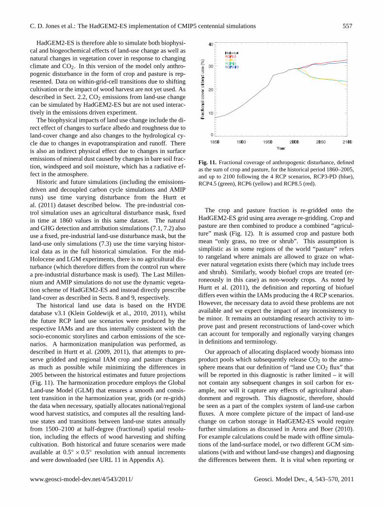
The historical land use data is based on the HYDEdatabase v3.1 (Klein Goldewijk et al., 2010, 2011), whilstthe future RCP land use scenarios were produced by therespective IAMs and are thus internally consistent with thesocio-economic storylines and carbon emissions of the sce-narios. A harmonization manipulation was performed, asdescribed in Hurtt et al. (2009, 2011), that attempts to pre-serve gridded and regional IAM crop and pasture changesas much as possible while minimizing the differences in2005 between the historical estimates and future projections(Fig. 11). The harmonization procedure employs the GlobalLand-use Model (GLM) that ensures a smooth and consis-tent transition in the harmonization year, grids (or re-grids)the data when necessary, spatially allocates national/regionalwood harvest statistics, and computes all the resulting land-use states and transitions between land-use states annuallyfrom 1500–2100 at half-degree (fractional) spatial resolu-tion, including the effects of wood harvesting and shiftingcultivation. Both historical and future scenarios were madeavailable at 0.5◦ × 0.5◦ resolution with annual incrementsand were downloaded (see URL 11 in Appendix A).
Fig. 11. Fractional coverage of anthropogenic disturbance, definedas the sum of crop and pasture, for the historical period 1860–2005,and up to 2100 following the 4 RCP scenarios, RCP3-PD (blue),RCP4.5 (green), RCP6 (yellow) and RCP8.5 (red).
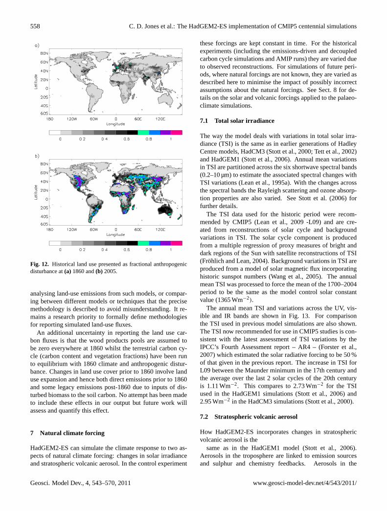
The crop and pasture fraction is re-gridded onto theHadGEM2-ES grid using area average re-gridding. Crop andpasture are then combined to produce a combined “agricul-ture” mask (Fig. 12). It is assumed crop and pasture bothmean “only grass, no tree or shrub”. This assumption issimplistic as in some regions of the world “pasture” refersto rangeland where animals are allowed to graze on what-ever natural vegetation exists there (which may include treesand shrub). Similarly, woody biofuel crops are treated (er-roneously in this case) as non-woody crops. As noted byHurtt et al. (2011), the definition and reporting of biofueldiffers even within the IAMs producing the 4 RCP scenarios.However, the necessary data to avoid these problems are notavailable and we expect the impact of any inconsistency tobe minor. It remains an outstanding research activity to im-prove past and present reconstructions of land-cover whichcan account for temporally and regionally varying changesin definitions and terminology.
Our approach of allocating displaced woody biomass intoproduct pools which subsequently release CO2 to the atmo-sphere means that our definition of “land use CO2 flux” thatwill be reported in this diagnostic is rather limited – it willnot contain any subsequent changes in soil carbon for ex-ample, nor will it capture any effects of agricultural aban-donment and regrowth. This diagnostic, therefore, shouldbe seen as a part of the complex system of land-use carbonfluxes. A more complete picture of the impact of land-usechange on carbon storage in HadGEM2-ES would requirefurther simulations as discussed in Arora and Boer (2010).For example calculations could be made with offline simula-tions of the land-surface model, or two different GCM sim-ulations (with and without land-use changes) and diagnosingthe differences between them. It is vital when reporting or
www.geosci-model-dev.net/4/543/2011/ Geosci. Model Dev., 4, 543–570, 2011
558 C. D. Jones et al.: The HadGEM2-ES implementation of CMIP5 centennial simulations
Fig. 12. Historical land use presented as fractional anthropogenicdisturbance at(a) 1860 and(b) 2005.
analysing land-use emissions from such models, or compar-ing between different models or techniques that the precisemethodology is described to avoid misunderstanding. It re-mains a research priority to formally define methodologiesfor reporting simulated land-use fluxes.
An additional uncertainty in reporting the land use car-bon fluxes is that the wood products pools are assumed tobe zero everywhere at 1860 whilst the terrestrial carbon cy-cle (carbon content and vegetation fractions) have been runto equilibrium with 1860 climate and anthropogenic distur-bance. Changes in land use cover prior to 1860 involve landuse expansion and hence both direct emissions prior to 1860and some legacy emissions post-1860 due to inputs of dis-turbed biomass to the soil carbon. No attempt has been madeto include these effects in our output but future work willassess and quantify this effect.
7 Natural climate forcing
HadGEM2-ES can simulate the climate response to two as-pects of natural climate forcing: changes in solar irradianceand stratospheric volcanic aerosol. In the control experiment
these forcings are kept constant in time. For the historicalexperiments (including the emissions-driven and decoupledcarbon cycle simulations and AMIP runs) they are varied dueto observed reconstructions. For simulations of future peri-ods, where natural forcings are not known, they are varied asdescribed here to minimise the impact of possibly incorrectassumptions about the natural forcings. See Sect. 8 for de-tails on the solar and volcanic forcings applied to the palaeo-climate simulations.
7.1 Total solar irradiance
The way the model deals with variations in total solar irra-diance (TSI) is the same as in earlier generations of HadleyCentre models, HadCM3 (Stott et al., 2000; Tett et al., 2002)and HadGEM1 (Stott et al., 2006). Annual mean variationsin TSI are partitioned across the six shortwave spectral bands(0.2–10 µm) to estimate the associated spectral changes withTSI variations (Lean et al., 1995a). With the changes acrossthe spectral bands the Rayleigh scattering and ozone absorp-tion properties are also varied. See Stott et al. (2006) forfurther details.
The TSI data used for the historic period were recom-mended by CMIP5 (Lean et al., 2009 -L09) and are cre-ated from reconstructions of solar cycle and backgroundvariations in TSI. The solar cycle component is producedfrom a multiple regression of proxy measures of bright anddark regions of the Sun with satellite reconstructions of TSI(Frohlich and Lean, 2004). Background variations in TSI areproduced from a model of solar magnetic flux incorporatinghistoric sunspot numbers (Wang et al., 2005). The annualmean TSI was processed to force the mean of the 1700–2004period to be the same as the model control solar constantvalue (1365 Wm−2).
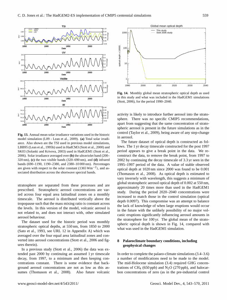
The annual mean TSI and variations across the UV, vis-ible and IR bands are shown in Fig. 13. For comparisonthe TSI used in previous model simulations are also shown.The TSI now recommended for use in CMIP5 studies is con-sistent with the latest assessment of TSI variations by theIPCC’s Fourth Assessment report – AR4 – (Forster et al.,2007) which estimated the solar radiative forcing to be 50 %of that given in the previous report. The increase in TSI forL09 between the Maunder minimum in the 17th century andthe average over the last 2 solar cycles of the 20th centuryis 1.11 Wm−2. This compares to 2.73 Wm−2 for the TSIused in the HadGEM1 simulations (Stott et al., 2006) and2.95 Wm−2 in the HadCM3 simulations (Stott et al., 2000).
7.2 Stratospheric volcanic aerosol
How HadGEM2-ES incorporates changes in stratosphericvolcanic aerosol is the
same as in the HadGEM1 model (Stott et al., 2006).Aerosols in the troposphere are linked to emission sourcesand sulphur and chemistry feedbacks. Aerosols in the
Geosci. Model Dev., 4, 543–570, 2011 www.geosci-model-dev.net/4/543/2011/
C. D. Jones et al.: The HadGEM2-ES implementation of CMIP5 centennial simulations 559
TSI
1850 1900 1950 2000Date
1365
1366
1367
Wm
-2
TSI
1850 1900 1950 2000Date
-0.05
0.00
0.05
0.10
0.15
0.20
Per
cent
age
LBB95SK03L09
UV
1850 1900 1950 2000Date
29.2
29.3
29.4
29.5
Wm
-2
UV
1850 1900 1950 2000Date
-0.2
0.0
0.2
0.4
0.6
0.8
Per
cent
age
Visible
1850 1900 1950 2000Date
594.5
595.0
595.5
Wm
-2
Visible
1850 1900 1950 2000Date
0.00
0.05
0.10
Per
cent
age
IR
1850 1900 1950 2000Date
740.8
741.0
741.2
741.4
Wm
-2
IR
1850 1900 1950 2000Date
-0.02
0.00
0.02
0.04
0.06
0.08P
erce
ntag
e
Fig. 13.Annual mean solar irradiance variations used in the historicmodel simulation (L09 - Lean et al., 2009).(a) Total solar irradi-ance. Also shown are the TSI used in previous model simulations,LBB95 (Lean et al., 1995b) used in HadCM3 (Stott et al., 2000) andSK03 (Solanki and Krivova, 2003) used in HadGEM1 (Stott et al.,2006). Solar irradiance averaged over(b) the ultraviolet band (200–320 nm),(c) the two visible bands (320–690 nm), and(d) infraredbands (690–1190, 1190–2380, and 2380–10 000 nm). Percentagesare given with respect to the solar constant (1365 Wm−2), and as-sociated distribution across the shortwave spectral bands.
stratosphere are separated from these processes and areprescribed. Stratospheric aerosol concentrations are var-ied across four equal area latitudinal zones on a monthlytimescale. The aerosol is distributed vertically above thetropopause such that the mass mixing ratio is constant acrossthe levels. In this version of the model, volcanic aerosol isnot related to, and does not interact with, other simulatedaerosol behaviour.
The dataset used for the historic period was monthlystratospheric optical depths, at 550 nm, from 1850 to 2000(Sato et al., 1993, see URL 12 in Appendix A) which wasaveraged over the four equal area latitudinal zones and con-verted into aerosol concentrations (Stott et al., 2006 and fig-ures therein).
In a previous study (Stott et al., 2006) the data was ex-tended past 2000 by continuing an assumed 1 yr timescaledecay, from 1997, to a minimum and then keeping con-centrations constant. There is some evidence that back-ground aerosol concentrations are not as low as this as-sumes (Thomason et al., 2008). Also future volcanic
Global mean optical depth
1990 2000 2010 2020 2030 2040
1
10
100
1000
optic
al d
epth
x 1
0000
.
This studyStott 2006 study
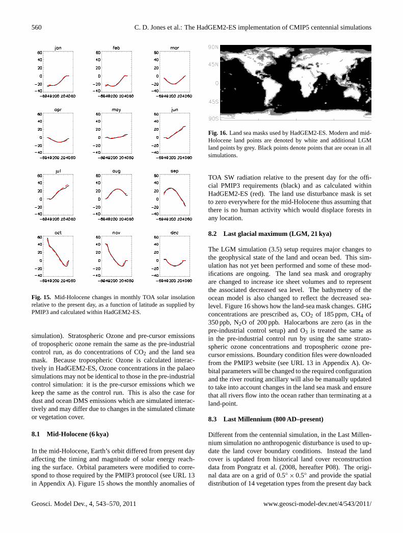
Fig. 14. Monthly global mean stratospheric optical depth as usedin this study and what was included in the HadGEM1 simulations(Stott, 2006), for the period 1990–2040.
activity is likely to introduce further aerosol into the strato-sphere. There was no specific CMIP5 recommendations,apart from suggesting that the same concentration of strato-spheric aerosol is present in the future simulations as in thecontrol (Taylor et al., 2009), being aware of any step-changein aerosol.
The future dataset of optical depth is constructed as fol-lows. The 1 yr decay timescale constructed for the post 1997period appears to give a break point in the data. We re-construct the data, to remove the break point, from 1997 to2002 by continuing the decay timescale of 3.3 yr seen in the1995–1997 period of the data. A value of stable observedoptical depth at 1020 nm since 2000 was found to be 0.001(Thomason et al., 2008). As optical depth is estimated tovary inversely with wavelength, this suggests a minimum ofglobal stratospheric aerosol optical depth of 0.002 at 550 nm,approximately 20 times more than used in the HadGEM1study. During the period 2020–2040 concentrations wereincreased to match those in the control simulation (opticaldepth 0.0097). This compromise was an attempt to balancethe lack of knowledge of when large eruptions would occurin the future with the unlikely possibility of no major vol-canic eruptions significantly influencing aerosol amounts inthe stratosphere for 100 yr. The global mean of the strato-spheric optical depth is shown in Fig. 14, compared withwhat was used in the HadGEM1 simulation.
8 Palaeoclimate boundary conditions, includinggeophysical changes
In order to complete the palaeo-climate simulations (3.4–3.6)a number of modifications need to be made to the model.The mid-Holocene simulation (3.4) required GHG concen-trations of CH4 (650 ppb) and N2O (270 ppb), and halocar-bon concentrations of zero (as in the pre-industrial control
www.geosci-model-dev.net/4/543/2011/ Geosci. Model Dev., 4, 543–570, 2011
560 C. D. Jones et al.: The HadGEM2-ES implementation of CMIP5 centennial simulations
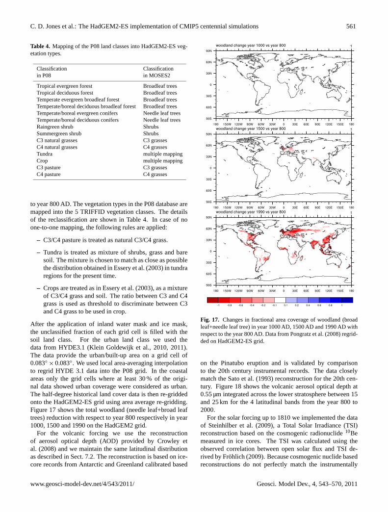
Fig. 15. Mid-Holocene changes in monthly TOA solar insolationrelative to the present day, as a function of latitude as supplied byPMIP3 and calculated within HadGEM2-ES.
simulation). Stratospheric Ozone and pre-cursor emissionsof tropospheric ozone remain the same as the pre-industrialcontrol run, as do concentrations of CO2 and the land seamask. Because tropospheric Ozone is calculated interac-tively in HadGEM2-ES, Ozone concentrations in the palaeosimulations may not be identical to those in the pre-industrialcontrol simulation: it is the pre-cursor emissions which wekeep the same as the control run. This is also the case fordust and ocean DMS emissions which are simulated interac-tively and may differ due to changes in the simulated climateor vegetation cover.
8.1 Mid-Holocene (6 kya)
In the mid-Holocene, Earth’s orbit differed from present dayaffecting the timing and magnitude of solar energy reach-ing the surface. Orbital parameters were modified to corre-spond to those required by the PMIP3 protocol (see URL 13in Appendix A). Figure 15 shows the monthly anomalies of
Fig. 16. Land sea masks used by HadGEM2-ES. Modern and mid-Holocene land points are denoted by white and additional LGMland points by grey. Black points denote points that are ocean in allsimulations.
TOA SW radiation relative to the present day for the offi-cial PMIP3 requirements (black) and as calculated withinHadGEM2-ES (red). The land use disturbance mask is setto zero everywhere for the mid-Holocene thus assuming thatthere is no human activity which would displace forests inany location.
8.2 Last glacial maximum (LGM, 21 kya)
The LGM simulation (3.5) setup requires major changes tothe geophysical state of the land and ocean bed. This sim-ulation has not yet been performed and some of these mod-ifications are ongoing. The land sea mask and orographyare changed to increase ice sheet volumes and to representthe associated decreased sea level. The bathymetry of theocean model is also changed to reflect the decreased sea-level. Figure 16 shows how the land-sea mask changes. GHGconcentrations are prescribed as, CO2 of 185 ppm, CH4 of350 ppb, N2O of 200 ppb. Halocarbons are zero (as in thepre-industrial control setup) and O3 is treated the same asin the pre-industrial control run by using the same strato-spheric ozone concentrations and tropospheric ozone pre-cursor emissions. Boundary condition files were downloadedfrom the PMIP3 website (see URL 13 in Appendix A). Or-bital parameters will be changed to the required configurationand the river routing ancillary will also be manually updatedto take into account changes in the land sea mask and ensurethat all rivers flow into the ocean rather than terminating at aland-point.
8.3 Last Millennium (800 AD–present)
Different from the centennial simulation, in the Last Millen-nium simulation no anthropogenic disturbance is used to up-date the land cover boundary conditions. Instead the landcover is updated from historical land cover reconstructiondata from Pongratz et al. (2008, hereafter P08). The origi-nal data are on a grid of 0.5◦
× 0.5◦ and provide the spatialdistribution of 14 vegetation types from the present day back
Geosci. Model Dev., 4, 543–570, 2011 www.geosci-model-dev.net/4/543/2011/
C. D. Jones et al.: The HadGEM2-ES implementation of CMIP5 centennial simulations 561
Table 4. Mapping of the P08 land classes into HadGEM2-ES veg-etation types.
Classification Classificationin P08 in MOSES2
Tropical evergreen forest Broadleaf treesTropical deciduous forest Broadleaf treesTemperate evergreen broadleaf forest Broadleaf treesTemperate/boreal deciduous broadleaf forest Broadleaf treesTemperate/boreal evergreen conifers Needle leaf treesTemperate/boreal deciduous conifers Needle leaf treesRaingreen shrub ShrubsSummergreen shrub ShrubsC3 natural grasses C3 grassesC4 natural grasses C4 grassesTundra multiple mappingCrop multiple mappingC3 pasture C3 grassesC4 pasture C4 grasses
to year 800 AD. The vegetation types in the P08 database aremapped into the 5 TRIFFID vegetation classes. The detailsof the reclassification are shown in Table 4. In case of noone-to-one mapping, the following rules are applied:
– C3/C4 pasture is treated as natural C3/C4 grass.
– Tundra is treated as mixture of shrubs, grass and baresoil. The mixture is chosen to match as close as possiblethe distribution obtained in Essery et al. (2003) in tundraregions for the present time.
– Crops are treated as in Essery et al. (2003), as a mixtureof C3/C4 grass and soil. The ratio between C3 and C4grass is used as threshold to discriminate between C3and C4 grass to be used in crop.
After the application of inland water mask and ice mask,the unclassified fraction of each grid cell is filled with thesoil land class. For the urban land class we used thedata from HYDE3.1 (Klein Goldewijk et al., 2010, 2011).The data provide the urban/built-up area on a grid cell of0.083◦ × 0.083◦. We used local area-averaging interpolationto regrid HYDE 3.1 data into the P08 grid. In the coastalareas only the grid cells where at least 30 % of the origi-nal data showed urban coverage were considered as urban.The half-degree historical land cover data is then re-griddedonto the HadGEM2-ES grid using area average re-gridding.Figure 17 shows the total woodland (needle leaf+broad leaftrees) reduction with respect to year 800 respectively in year1000, 1500 and 1990 on the HadGEM2 grid.
For the volcanic forcing we use the reconstructionof aerosol optical depth (AOD) provided by Crowley etal. (2008) and we maintain the same latitudinal distributionas described in Sect. 7.2. The reconstruction is based on ice-core records from Antarctic and Greenland calibrated based
Fig. 17. Changes in fractional area coverage of woodland (broadleaf+needle leaf tree) in year 1000 AD, 1500 AD and 1990 AD withrespect to the year 800 AD. Data from Pongratz et al. (2008) regrid-ded on HadGEM2-ES grid.
on the Pinatubo eruption and is validated by comparisonto the 20th century instrumental records. The data closelymatch the Sato et al. (1993) reconstruction for the 20th cen-tury. Figure 18 shows the volcanic aerosol optical depth at0.55 µm integrated across the lower stratosphere between 15and 25 km for the 4 latitudinal bands from the year 800 to2000.
For the solar forcing up to 1810 we implemented the dataof Steinhilber et al. (2009), a Total Solar Irradiance (TSI)reconstruction based on the cosmogenic radionuclide10Bemeasured in ice cores. The TSI was calculated using theobserved correlation between open solar flux and TSI de-rived by Frohlich (2009). Because cosmogenic nuclide basedreconstructions do not perfectly match the instrumentally
www.geosci-model-dev.net/4/543/2011/ Geosci. Model Dev., 4, 543–570, 2011
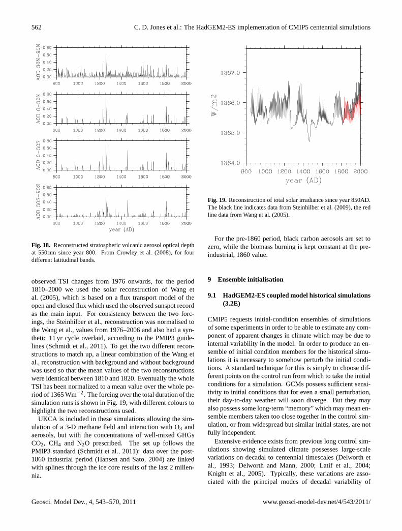
562 C. D. Jones et al.: The HadGEM2-ES implementation of CMIP5 centennial simulations
Fig. 18. Reconstructed stratospheric volcanic aerosol optical depthat 550 nm since year 800. From Crowley et al. (2008), for fourdifferent latitudinal bands.
observed TSI changes from 1976 onwards, for the period1810–2000 we used the solar reconstruction of Wang etal. (2005), which is based on a flux transport model of theopen and closed flux which used the observed sunspot recordas the main input. For consistency between the two forc-ings, the Steinhilber et al., reconstruction was normalised tothe Wang et al., values from 1976–2006 and also had a syn-thetic 11 yr cycle overlaid, according to the PMIP3 guide-lines (Schmidt et al., 2011). To get the two different recon-structions to match up, a linear combination of the Wang etal., reconstruction with background and without backgroundwas used so that the mean values of the two reconstructionswere identical between 1810 and 1820. Eventually the wholeTSI has been normalized to a mean value over the whole pe-riod of 1365 Wm−2. The forcing over the total duration of thesimulation runs is shown in Fig. 19, with different colours tohighlight the two reconstructions used.
UKCA is included in these simulations allowing the sim-ulation of a 3-D methane field and interaction with O3 andaerosols, but with the concentrations of well-mixed GHGsCO2, CH4 and N2O prescribed. The set up follows thePMIP3 standard (Schmidt et al., 2011): data over the post-1860 industrial period (Hansen and Sato, 2004) are linkedwith splines through the ice core results of the last 2 millen-nia.
Fig. 19. Reconstruction of total solar irradiance since year 850AD.The black line indicates data from Steinhilber et al. (2009), the redline data from Wang et al. (2005).
For the pre-1860 period, black carbon aerosols are set tozero, while the biomass burning is kept constant at the pre-industrial, 1860 value.
9 Ensemble initialisation
9.1 HadGEM2-ES coupled model historical simulations(3.2E)
CMIP5 requests initial-condition ensembles of simulationsof some experiments in order to be able to estimate any com-ponent of apparent changes in climate which may be due tointernal variability in the model. In order to produce an en-semble of initial condition members for the historical simu-lations it is necessary to somehow perturb the initial condi-tions. A standard technique for this is simply to choose dif-ferent points on the control run from which to take the initialconditions for a simulation. GCMs possess sufficient sensi-tivity to initial conditions that for even a small perturbation,their day-to-day weather will soon diverge. But they mayalso possess some long-term “memory” which may mean en-semble members taken too close together in the control sim-ulation, or from widespread but similar initial states, are notfully independent.
Extensive evidence exists from previous long control sim-ulations showing simulated climate possesses large-scalevariations on decadal to centennial timescales (Delworth etal., 1993; Delworth and Mann, 2000; Latif et al., 2004;Knight et al., 2005). Typically, these variations are asso-ciated with the principal modes of decadal variability of
Geosci. Model Dev., 4, 543–570, 2011 www.geosci-model-dev.net/4/543/2011/
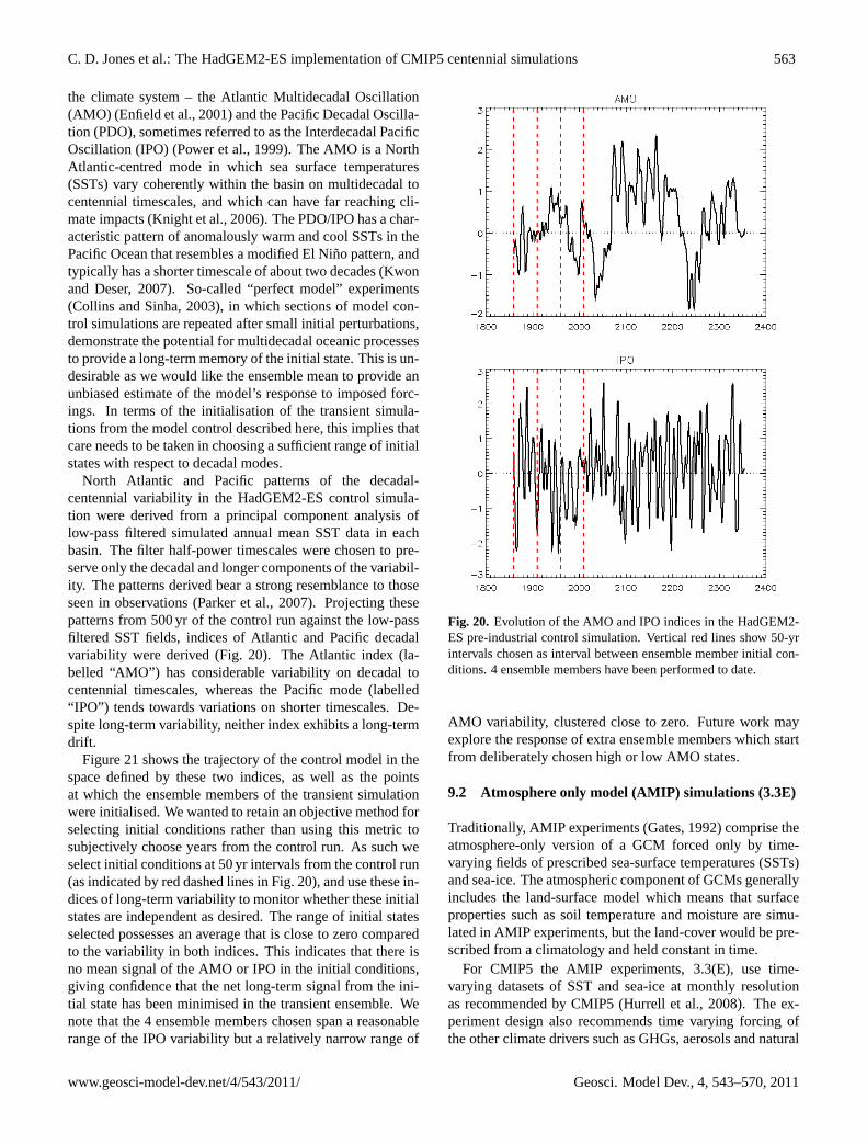
C. D. Jones et al.: The HadGEM2-ES implementation of CMIP5 centennial simulations 563
the climate system – the Atlantic Multidecadal Oscillation(AMO) (Enfield et al., 2001) and the Pacific Decadal Oscilla-tion (PDO), sometimes referred to as the Interdecadal PacificOscillation (IPO) (Power et al., 1999). The AMO is a NorthAtlantic-centred mode in which sea surface temperatures(SSTs) vary coherently within the basin on multidecadal tocentennial timescales, and which can have far reaching cli-mate impacts (Knight et al., 2006). The PDO/IPO has a char-acteristic pattern of anomalously warm and cool SSTs in thePacific Ocean that resembles a modified El Nino pattern, andtypically has a shorter timescale of about two decades (Kwonand Deser, 2007). So-called “perfect model” experiments(Collins and Sinha, 2003), in which sections of model con-trol simulations are repeated after small initial perturbations,demonstrate the potential for multidecadal oceanic processesto provide a long-term memory of the initial state. This is un-desirable as we would like the ensemble mean to provide anunbiased estimate of the model’s response to imposed forc-ings. In terms of the initialisation of the transient simula-tions from the model control described here, this implies thatcare needs to be taken in choosing a sufficient range of initialstates with respect to decadal modes.
North Atlantic and Pacific patterns of the decadal-centennial variability in the HadGEM2-ES control simula-tion were derived from a principal component analysis oflow-pass filtered simulated annual mean SST data in eachbasin. The filter half-power timescales were chosen to pre-serve only the decadal and longer components of the variabil-ity. The patterns derived bear a strong resemblance to thoseseen in observations (Parker et al., 2007). Projecting thesepatterns from 500 yr of the control run against the low-passfiltered SST fields, indices of Atlantic and Pacific decadalvariability were derived (Fig. 20). The Atlantic index (la-belled “AMO”) has considerable variability on decadal tocentennial timescales, whereas the Pacific mode (labelled“IPO”) tends towards variations on shorter timescales. De-spite long-term variability, neither index exhibits a long-termdrift.
Figure 21 shows the trajectory of the control model in thespace defined by these two indices, as well as the pointsat which the ensemble members of the transient simulationwere initialised. We wanted to retain an objective method forselecting initial conditions rather than using this metric tosubjectively choose years from the control run. As such weselect initial conditions at 50 yr intervals from the control run(as indicated by red dashed lines in Fig. 20), and use these in-dices of long-term variability to monitor whether these initialstates are independent as desired. The range of initial statesselected possesses an average that is close to zero comparedto the variability in both indices. This indicates that there isno mean signal of the AMO or IPO in the initial conditions,giving confidence that the net long-term signal from the ini-tial state has been minimised in the transient ensemble. Wenote that the 4 ensemble members chosen span a reasonablerange of the IPO variability but a relatively narrow range of
Fig. 20. Evolution of the AMO and IPO indices in the HadGEM2-ES pre-industrial control simulation. Vertical red lines show 50-yrintervals chosen as interval between ensemble member initial con-ditions. 4 ensemble members have been performed to date.
AMO variability, clustered close to zero. Future work mayexplore the response of extra ensemble members which startfrom deliberately chosen high or low AMO states.
9.2 Atmosphere only model (AMIP) simulations (3.3E)
Traditionally, AMIP experiments (Gates, 1992) comprise theatmosphere-only version of a GCM forced only by time-varying fields of prescribed sea-surface temperatures (SSTs)and sea-ice. The atmospheric component of GCMs generallyincludes the land-surface model which means that surfaceproperties such as soil temperature and moisture are simu-lated in AMIP experiments, but the land-cover would be pre-scribed from a climatology and held constant in time.
For CMIP5 the AMIP experiments, 3.3(E), use time-varying datasets of SST and sea-ice at monthly resolutionas recommended by CMIP5 (Hurrell et al., 2008). The ex-periment design also recommends time varying forcing ofthe other climate drivers such as GHGs, aerosols and natural
www.geosci-model-dev.net/4/543/2011/ Geosci. Model Dev., 4, 543–570, 2011
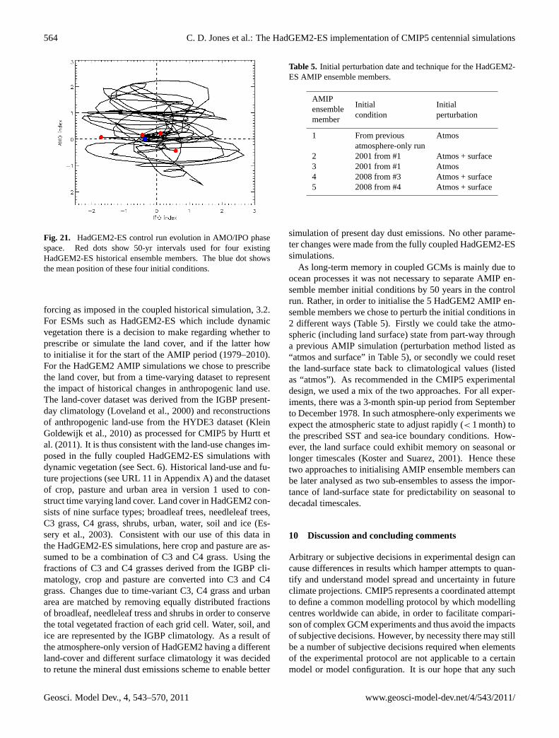
564 C. D. Jones et al.: The HadGEM2-ES implementation of CMIP5 centennial simulations
Fig. 21. HadGEM2-ES control run evolution in AMO/IPO phasespace. Red dots show 50-yr intervals used for four existingHadGEM2-ES historical ensemble members. The blue dot showsthe mean position of these four initial conditions.
forcing as imposed in the coupled historical simulation, 3.2.For ESMs such as HadGEM2-ES which include dynamicvegetation there is a decision to make regarding whether toprescribe or simulate the land cover, and if the latter howto initialise it for the start of the AMIP period (1979–2010).For the HadGEM2 AMIP simulations we chose to prescribethe land cover, but from a time-varying dataset to representthe impact of historical changes in anthropogenic land use.The land-cover dataset was derived from the IGBP present-day climatology (Loveland et al., 2000) and reconstructionsof anthropogenic land-use from the HYDE3 dataset (KleinGoldewijk et al., 2010) as processed for CMIP5 by Hurtt etal. (2011). It is thus consistent with the land-use changes im-posed in the fully coupled HadGEM2-ES simulations withdynamic vegetation (see Sect. 6). Historical land-use and fu-ture projections (see URL 11 in Appendix A) and the datasetof crop, pasture and urban area in version 1 used to con-struct time varying land cover. Land cover in HadGEM2 con-sists of nine surface types; broadleaf trees, needleleaf trees,C3 grass, C4 grass, shrubs, urban, water, soil and ice (Es-sery et al., 2003). Consistent with our use of this data inthe HadGEM2-ES simulations, here crop and pasture are as-sumed to be a combination of C3 and C4 grass. Using thefractions of C3 and C4 grasses derived from the IGBP cli-matology, crop and pasture are converted into C3 and C4grass. Changes due to time-variant C3, C4 grass and urbanarea are matched by removing equally distributed fractionsof broadleaf, needleleaf tress and shrubs in order to conservethe total vegetated fraction of each grid cell. Water, soil, andice are represented by the IGBP climatology. As a result ofthe atmosphere-only version of HadGEM2 having a differentland-cover and different surface climatology it was decidedto retune the mineral dust emissions scheme to enable better
Table 5. Initial perturbation date and technique for the HadGEM2-ES AMIP ensemble members.
AMIPInitial Initialensemblecondition perturbationmember
1 From previous Atmosatmosphere-only run
2 2001 from #1 Atmos + surface3 2001 from #1 Atmos4 2008 from #3 Atmos + surface5 2008 from #4 Atmos + surface
simulation of present day dust emissions. No other parame-ter changes were made from the fully coupled HadGEM2-ESsimulations.
As long-term memory in coupled GCMs is mainly due toocean processes it was not necessary to separate AMIP en-semble member initial conditions by 50 years in the controlrun. Rather, in order to initialise the 5 HadGEM2 AMIP en-semble members we chose to perturb the initial conditions in2 different ways (Table 5). Firstly we could take the atmo-spheric (including land surface) state from part-way througha previous AMIP simulation (perturbation method listed as“atmos and surface” in Table 5), or secondly we could resetthe land-surface state back to climatological values (listedas “atmos”). As recommended in the CMIP5 experimentaldesign, we used a mix of the two approaches. For all exper-iments, there was a 3-month spin-up period from Septemberto December 1978. In such atmosphere-only experiments weexpect the atmospheric state to adjust rapidly (< 1 month) tothe prescribed SST and sea-ice boundary conditions. How-ever, the land surface could exhibit memory on seasonal orlonger timescales (Koster and Suarez, 2001). Hence thesetwo approaches to initialising AMIP ensemble members canbe later analysed as two sub-ensembles to assess the impor-tance of land-surface state for predictability on seasonal todecadal timescales.
10 Discussion and concluding comments
Arbitrary or subjective decisions in experimental design cancause differences in results which hamper attempts to quan-tify and understand model spread and uncertainty in futureclimate projections. CMIP5 represents a coordinated attemptto define a common modelling protocol by which modellingcentres worldwide can abide, in order to facilitate compari-son of complex GCM experiments and thus avoid the impactsof subjective decisions. However, by necessity there may stillbe a number of subjective decisions required when elementsof the experimental protocol are not applicable to a certainmodel or model configuration. It is our hope that any such
Geosci. Model Dev., 4, 543–570, 2011 www.geosci-model-dev.net/4/543/2011/
C. D. Jones et al.: The HadGEM2-ES implementation of CMIP5 centennial simulations 565
occurrences with HadGEM2-ES will not have a large impacton the interpretation of the results, but we discuss here forcompleteness some possible impacts.
In the HadGEM2-ES earth system model (Collins et al.,2011), some of the components of the earth system arenow simulated interactively by the model rather than be-ing prescribed as external boundary conditions. For exam-ple, HadGEM2-ES includes interactive tropospheric chem-istry and hence can simulate the evolution of atmosphericmethane and ozone concentration in response to meteorolog-ical conditions and emissions of reactive gases. Therefore at-mospheric composition may not follow exactly the CMIP5-prescribed values. In our experiments we have forced thesurface methane concentrations to follow the CMIP5 valuesin order to reduce any model drift away from the scenarios,but there may still be differences in CH4 concentrations inthe free atmosphere away from the surface.
Similarly, simulated tropospheric ozone may not followthe exact CMIP5-prescribed concentrations. In general, wesee this enhanced, process-based functionality of the modelas a benefit – the rationale behind developing such a complexearth system model is precisely to study these interactionsand allow them to change consistently with future climatein a way not possible with prescribed concentrations. Butwe do acknowledge that these differences also represent adivergence from the precise CMIP5 protocol which shouldbe borne in mind during subsequent multi-model analysis.
Other areas where a divergence may occur due to the struc-ture of the ESM include land-use forcing and set-up of detec-tion and attribution experiments.
By prescribing anthropogenic disturbance in addition tosimulated, dynamic vegetation we risk diverging from theintended impact of the prescribed land-use change. For ex-ample, if the model initially simulates too much or too littleforest in a region to be deforested then the impact of this de-forestation on both carbon storage and physical surface prop-erties will be too great or too little. We mitigate the risk ofthis impact in the emission-driven experiments by overwrit-ing the land-use flux seen by the atmosphere by the CMIP5-prescribed land-use emissions dataset. However, the issueremains for any biophysical effect of land-use change. Fu-ture work is required to quantify the impact of this effect.
Detection and attribution studies aim to attribute changesin observed climate to driving processes. Model experimentsare designed to do this by varying or holding constant sep-arate forcings such as natural, greenhouse gases or aerosols.In this way the characteristic spatial or temporal patterns ofresponse to each forcing can be derived and an optimal scal-ing found to best match observations. The scaling is thenused to deduce if the signal for the forcing is detected and ifthe scaled response is consistent with the original signal, thusproviding confidence for an attribution statement. In GCMsto date the distinction between, say, natural and greenhousegas forcing is clear, and it is easy in the model to hold onefixed whilst varying the other. However, in an ESM where
simulated GHG concentrations (such as methane or ozone)or aerosols may respond to climate, this distinction becomesslightly blurred. If natural forcings affect atmospheric pro-cesses which alter GHG or aerosol amounts then should thesebe allowed to vary or not in the “natural” detection and attri-bution experiment? Or should the HadGEM2-ES “natural”simulations be forced to solely consider the direct radiativeeffects of the natural forcings?
In the HadGEM2-ES natural experiment we varied the TSIand stratospheric volcanic aerosol concentrations as per thehistorical simulation, kept all other emissions/concentrationsthe same as in the control simulation and allowed the earthsystem processes to vary as normal. We decided on a morecomplicated set up for the GHG only forced run. Concentra-tions of the greenhouse gases (CO2, CH4, N2O and the halo-carbon species) were prescribed throughout the atmospherefor the radiation scheme. However, prescribing the methaneseen by the chemistry scheme would influence the chemistryand thus species like ozone, which we did not want to be var-ied in this experiment. So in the interactive chemistry partof the model, the set up was as in the control, i.e. methaneemissions at surface and concentrations in the atmosphere asin the control simulation. This “chemistry methane” does notinteract with the radiation scheme. Our choice to do this wastherefore a pragmatic compromise between the ESM part ofthe model and the needs of a detection and attribution study.
In this paper we have documented how we have imple-mented the CMIP5 experimental protocol for the centennialsimulations in the Met Office HadGEM2-ES earth systemmodel. We have successfully set-up and performed the ex-periments as described here and will make the results avail-able via the PCMDI multi-model database. We hope thesewill form a valuable contribution to the CMIP5 modellingactivity.
Appendix A
List of URLs / websites
1. The main CMIP5 web pagehttp://cmip-pcmdi.llnl.gov/cmip5/index.html
2. CMIP5 output guidelineshttp://cmip-pcmdi.llnl.gov/cmip5/outputreq.html
3. The RCP White Paper: document 8 at:http://cmip-pcmdi.llnl.gov/cmip5/modelingdocuments.html
4. The CO2 concentrations used were taken from theCMIP5 datasethttp://cmip-pcmdi.llnl.gov/cmip5/forcing.html
5. NOAA global mean CO2 dataftp://ftp.cmdl.noaa.gov/ccg/co2/trends/co2 annmeangl.txt
www.geosci-model-dev.net/4/543/2011/ Geosci. Model Dev., 4, 543–570, 2011
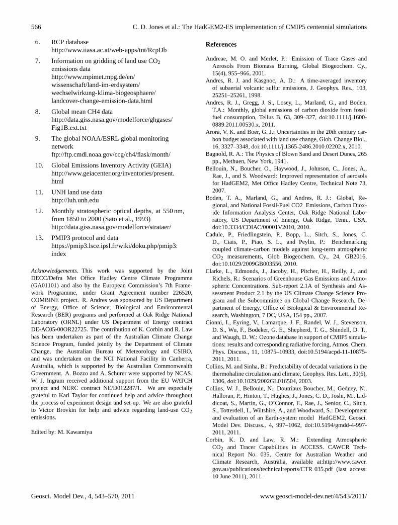
566 C. D. Jones et al.: The HadGEM2-ES implementation of CMIP5 centennial simulations
6. RCP databasehttp://www.iiasa.ac.at/web-apps/tnt/RcpDb
7. Information on gridding of land use CO2emissions datahttp://www.mpimet.mpg.de/en/wissenschaft/land-im-erdsystem/wechselwirkung-klima-biogeosphaere/landcover-change-emission-data.html
8. Global mean CH4 datahttp://data.giss.nasa.gov/modelforce/ghgases/Fig1B.ext.txt
9. The global NOAA/ESRL global monitoringnetworkftp://ftp.cmdl.noaa.gov/ccg/ch4/flask/month/
10. Global Emissions Inventory Activity (GEIA)http://www.geiacenter.org/inventories/present.html
11. UNH land use datahttp://luh.unh.edu
12. Monthly stratospheric optical depths, at 550 nm,from 1850 to 2000 (Sato et al., 1993)http://data.giss.nasa.gov/modelforce/strataer/
13. PMIP3 protocol and datahttps://pmip3.lsce.ipsl.fr/wiki/doku.php/pmip3:index
Acknowledgements.This work was supported by the JointDECC/Defra Met Office Hadley Centre Climate Programme(GA01101) and also by the European Commission’s 7th Frame-work Programme, under Grant Agreement number 226520,COMBINE project. R. Andres was sponsored by US Departmentof Energy, Office of Science, Biological and EnvironmentalResearch (BER) programs and performed at Oak Ridge NationalLaboratory (ORNL) under US Department of Energy contractDE-AC05-00OR22725. The contribution of K. Corbin and R. Lawhas been undertaken as part of the Australian Climate ChangeScience Program, funded jointly by the Department of ClimateChange, the Australian Bureau of Meteorology and CSIRO,and was undertaken on the NCI National Facility in Canberra,Australia, which is supported by the Australian CommonwealthGovernment. A. Bozzo and A. Schurer were supported by NCAS.W. J. Ingram received additional support from the EU WATCHproject and NERC contract NE/D012287/1. We are especiallygrateful to Karl Taylor for continued help and advice throughoutthe process of experiment design and set-up. We are also gratefulto Victor Brovkin for help and advice regarding land-use CO2emissions.
Edited by: M. Kawamiya
References
Andreae, M. O. and Merlet, P.: Emission of Trace Gases andAerosols From Biomass Burning, Global Biogeochem. Cy.,15(4), 955–966, 2001.
Andres, R. J. and Kasgnoc, A. D.: A time-averaged inventoryof subaerial volcanic sulfur emissions, J. Geophys. Res., 103,25251–25261, 1998.
Andres, R. J., Gregg, J. S., Losey, L., Marland, G., and Boden,T.A.: Monthly, global emissions of carbon dioxide from fossilfuel consumption, Tellus B, 63, 309–327,doi:10.1111/j.1600-0889.2011.00530.x, 2011.
Arora, V. K. and Boer, G. J.: Uncertainties in the 20th century car-bon budget associated with land use change, Glob. Change Biol.,16, 3327–3348,doi:10.1111/j.1365-2486.2010.02202.x, 2010.
Bagnold, R. A.: The Physics of Blown Sand and Desert Dunes, 265pp., Methuen, New York, 1941.
Bellouin, N., Boucher, O., Haywood, J., Johnson, C., Jones, A.,Rae, J., and S. Woodward: Improved representation of aerosolsfor HadGEM2, Met Office Hadley Centre, Technical Note 73,2007.
Boden, T. A., Marland, G., and Andres, R. J.: Global, Re-gional, and National Fossil-Fuel CO2 Emissions, Carbon Diox-ide Information Analysis Center, Oak Ridge National Labo-ratory, US Department of Energy, Oak Ridge, Tenn., USA,doi:10.3334/CDIAC/00001V2010, 2010.
Cadule, P., Friedlingstein, P., Bopp, L., Sitch, S., Jones, C.D., Ciais, P., Piao, S. L., and Peylin, P.: Benchmarkingcoupled climate-carbon models against long-term atmosphericCO2 measurements, Glob Biogeochem. Cy., 24, GB2016,doi:10.1029/2009GB003556, 2010.
Clarke, L., Edmonds, J., Jacoby, H., Pitcher, H., Reilly, J., andRichels, R.: Scenarios of Greenhouse Gas Emissions and Atmo-spheric Concentrations. Sub-report 2.1A of Synthesis and As-sessment Product 2.1 by the US Climate Change Science Pro-gram and the Subcommittee on Global Change Research, De-partment of Energy, Office of Biological & Environmental Re-search, Washington, 7 DC, USA, 154 pp., 2007.
Cionni, I., Eyring, V., Lamarque, J. F., Randel, W. J., Stevenson,D. S., Wu, F., Bodeker, G. E., Shepherd, T. G., Shindell, D. T.,and Waugh, D. W.: Ozone database in support of CMIP5 simula-tions: results and corresponding radiative forcing, Atmos. Chem.Phys. Discuss., 11, 10875–10933,doi:10.5194/acpd-11-10875-2011, 2011.
Collins, M. and Sinha, B.: Predictability of decadal variations in thethermohaline circulation and climate, Geophys. Res. Lett., 30(6),1306,doi:10.1029/2002GL016504, 2003.
Collins, W. J., Bellouin, N., Doutriaux-Boucher, M., Gedney, N.,Halloran, P., Hinton, T., Hughes, J., Jones, C. D., Joshi, M., Lid-dicoat, S., Martin, G., O’Connor, F., Rae, J., Senior, C., Sitch,S., Totterdell, I., Wiltshire, A., and Woodward, S.: Developmentand evaluation of an Earth-system model HadGEM2, Geosci.Model Dev. Discuss., 4, 997–1062,doi:10.5194/gmdd-4-997-2011, 2011.
Corbin, K. D. and Law, R. M.: Extending AtmosphericCO2 and Tracer Capabilities in ACCESS. CAWCR Tech-nical Report No. 035, Centre for Australian Weather andClimate Research, Australia, available at:http://www.cawcr.gov.au/publications/technicalreports/CTR035.pdf (last access:10 June 2011), 2011.
Geosci. Model Dev., 4, 543–570, 2011 www.geosci-model-dev.net/4/543/2011/
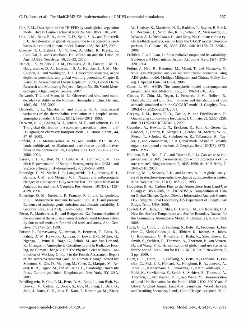
C. D. Jones et al.: The HadGEM2-ES implementation of CMIP5 centennial simulations 567
Cox, P. M.: Description of the TRIFFID dynamic global vegetationmodel. Hadley Centre Technical Note 24, Met Office, UK, 2001.
Cox, P. M., Betts, R. A., Jones, C. D., Spall, S. A., and Totterdell,I. J.: Acceleration of global warming due to carbon-cycle feed-backs in a coupled climate model, Nature, 408, 184–187, 2000.
Crowley, T. J., Zielinski, G., Vinther, B., Udisti, R., Kreutz, K.,Cole-Dai, J., and Castellano, E.: Volcanism and the Little IceAge, PAGES Newsletter, 16, 22–23, 2008.
Daniel, J. S., Velders, G. J. M., Douglass, A. R., Forster, P. M. D.,Hauglustaine, D. A., Isaksen, I. S. A., Kuijpers, L. J. M., Mc-Culloch, A., and Wallington, T. J.: Halocarbon scenarios, ozonedepletion potentials, and global warming potentials, Chapter 8,Scientific Assessment of Ozone Depletion: 2006, Global OzoneResearch and Monitoring Project – Report No. 50, World Mete-orological Organization, Geneva, 2007.
Delworth, T. L. and Mann, M. E.: Observed and simulated multi-decadal variability in the Northern Hemisphere, Clim. Dynam.,16(9), 661–676, 2000.
Delworth, T. L., Manabe, S., and Stouffer, R. J.: Interdecadalvariations of the thermohaline circulation in a coupled ocean-atmosphere model, J. Clim., 6(11), 1993–2011, 1993.
Derwent, R. G., Collins, W. J., Jenkin, M. E., and Johnson, C. E.:The global distribution of secondary particulate matter in a 3-D Lagrangian chemistry transport model, J. Atmos. Chem., 44,57–95, 2003.
Enfield, D. B., Mestas-Nunez, A. M., and Trimble, P.J.: The At-lantic multidecadal oscillation and its relation to rainfall and riverflows in the continental US, Geophys. Res. Lett., 28(10), 2077–2080, 2001.
Essery, R. L. H., Best, M. J., Betts, R. A., and Cox, P. M.: Ex-plicit Representation of Subgrid Heterogeneity in a GCM LandSurface Scheme, J. Hydrometeorol., 4, 530–543, 2003.
Etheridge, D. M., Steele, L. P., Langenfelds, R. L., Francey, R. J.,Barnola, J. M., and Morgan, V. I.: Natural and anthropogenicchanges in atmospheric CO2 over the last 1000 years from air inAntarctic ice and firn, J. Geophys. Res.-Atmos., 101(D2), 4115–4128, 1996.
Etheridge, D. M., Steele, L. P., Francey, R. J., and Langenfelds,R. L.: Atmospheric methane between 1000 A.D. and present:Evidence of anthropogenic emissions and climatic variability, J.Geophys. Res., 103(D13), 15979–15993, 1998.
Fecan, F., Marticorena, B., and Bergametti, G.: Parametrisation ofthe increase of the aeolian erosion threshold wind friction veloc-ity due to soil moisture for arid and semi-arid areas, Ann. Geo-phys. 17, 149–157, 1999.
Forster, P., Ramaswamy, V., Artaxo, P., Berntsen, T., Betts, R.,Fahey, D. W., Haywood, J., Lean, J., Lowe, D.C., Myhre, G.,Nganga, J., Prinn, R., Raga, G., Schulz, M., and Van Dorland,R.: Changes in Atmospheric Constituents and in Radiative Forc-ing, in: Climate Change 2007: The Physical Science Basis. Con-tribution of Working Group I to the Fourth Assessment Reportof the Intergovernmental Panel on Climate Change, edited by:Solomon, S., Qin, D., Manning, M., Chen, Z., Marquis, M., Av-eryt, K. B., Tignor, M., and Miller, H. L., Cambridge UniversityPress, Cambridge, United Kingdom and New York, NY, USA,2007.
Friedlingstein, P., Cox, P. M., Betts, R. A., Bopp, L., von Bloh, W.,Brovkin, V., Cadule, P., Doney, S., Eby, M., Fung, I., Bala, G.,John, J., Jones, C. D., Joos, F., Kato, T., Kawamiya, M., Knorr,
W., Lindsay, K., Matthews, H. D., Raddatz, T., Rayner, P., Reick,C., Roeckner, E., Schnitzler, K. G., Schnur, R., Strassmann, K.,Weaver, A. J., Yoshikawa, C., and Zeng, N.: Climate-carbon cy-cle feedback analysis, results from the C4MIP model intercom-parison, J. Climate, 19, 3337–3353,doi:10.1175/JCLI3800.1,2006.
Frohlich, C. and Lean, J.: Solar radiative output and its variability:Evidence and Mechanisms, Astron. Astrophys. Rev., 12(4), 273–320, 2004.
Fujino, J., Nair, R., Kainuma, M., Masui, T., and Matsuoka, Y.:Multi-gas mitigation analysis on stabilization scenarios usingAIM global model. Multigas Mitigation and Climate Policy, En-erg. J. Special Issue, 343–354, 2006.
Gates, L. W.: AMIP: The atmospheric model intercomparisonproject, Bull. Am. Meteorol. Soc., 73, 1962–1970, 1992.
Ginoux, P., Chin, M., Tegen, I., Prospero, J. M., Holben, B.,Dubovik, O., and Lin, S.-J.: Sources and distributions of dustaerosols simulated with the GOCART model, J. Geophys.-Res.,106(D17), 20255–20273, 2001.
Gregory, J. M., Jones, C. D., Cadule, P., and Friedlingstein, P.:Quantifying carbon-cycle feedbacks, J. Climate, 22, 5232–5250,doi:10.1175/2009JCLI2949.1, 2009.
Guenther, A., Hewitt, C. N., Erickson, D., Fall, R., Geron, C.,Graedel, T., Harley, P., Klinger, L., Lerdau, M., McKay, W. A.,Pierce, T., Scholes, B., Steinbrecher, R., Tallamraju, R., Tay-lor, J., and Zimmerman, P.: A global model of natural volatileorganic compound emissions, J. Geophys. Res., 100(D5), 8873–8892, 1995.
Halloran, P. R., Bell, T. G., and Totterdell, I. J.: Can we trust em-pirical marine DMS parameterisations within projections of fu-ture climate?, Biogeosciences, 7, 1645–1656,doi:10.5194/bg-7-1645-2010, 2010.
Hoerling, M. P., Schaack, T. K., and Lenzen, A. J.: A global analy-sis of stratosphere-tropospheric exchange during northern winter,Mon. Weather Rev., 121(1), 162–172, 1993.
Houghton, R. A.: Carbon Flux to the Atmosphere from Land-UseChanges: 1850–2005, in: TRENDS: A Compendium of Dataon Global Change. Carbon Dioxide Information Analysis Center,Oak Ridge National Laboratory, US Department of Energy, OakRidge, Tenn., USA, 2008.
Hurrell, J. W., Hack, J. J., Shea, D., Caron, J. M., and Rosinski, J.: ANew Sea Surface Temperature and Sea Ice Boundary Dataset forthe Community Atmosphere Model, J. Climate, 21, 5145–5153,2008.
Hurtt, G. C., Chini, L. P., Frolking, S., Betts, R., Feddema, J., Fis-cher, G., Klein Goldewijk, K., Hibbard, K., Janetos, A., Jones,C., Kindermann, G., Kinoshita, T., Riahi, K., Shevliakova, E.,Smith, S., Stehfest, E., Thomson, A., Thornton, P., van Vuuren,D., and Wang, Y. P.: Harmonisation of global land-use scenariosfor the period 1500–2100 for IPCC-AR5, iLEAPS Newsletter, 7,3 pp., 2009.
Hurtt, G. C., Chini, L. P., Frolking, S., Betts, R., Feddema, J., Fis-cher, G., Fisk, J. P., Hibbard, K., Houghton, R. A., Janetos, A.,Jones, C., Kindermann, G., Kinoshita, T., Klein Goldewijk, K.,Riahi, K., Shevliakova, E., Smith, S., Stehfest, E., Thomson, A.,Thornton, P., van Vuuren, D. P., and Wang, Y.: Harmonizationof Land-Use Scenarios for the Period 1500–2100: 600 Years ofGlobal Gridded Annual Land-Use Transitions, Wood Harvest,and Resulting Secondary Lands, Clim. Change, accepted, 2011.
www.geosci-model-dev.net/4/543/2011/ Geosci. Model Dev., 4, 543–570, 2011
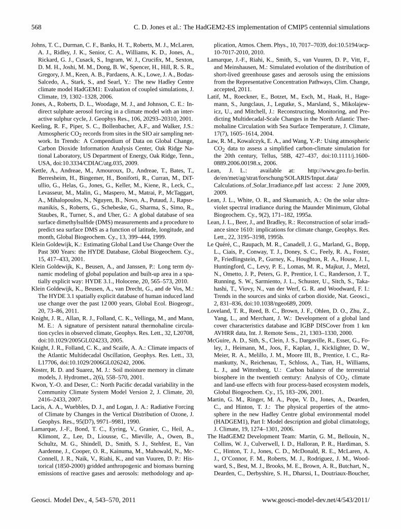
568 C. D. Jones et al.: The HadGEM2-ES implementation of CMIP5 centennial simulations
Johns, T. C., Durman, C. F., Banks, H. T., Roberts, M. J., McLaren,A. J., Ridley, J. K., Senior, C. A., Williams, K. D., Jones, A.,Rickard, G. J., Cusack, S., Ingram, W. J., Crucifix, M., Sexton,D. M. H., Joshi, M. M., Dong, B. W., Spencer, H., Hill, R. S. R.,Gregory, J. M., Keen, A. B., Pardaens, A. K., Lowe, J. A., Bodas-Salcedo, A., Stark, S., and Searl, Y.: The new Hadley Centreclimate model HadGEM1: Evaluation of coupled simulations, J.Climate, 19, 1302–1328, 2006.
Jones, A., Roberts, D. L., Woodage, M. J., and Johnson, C. E.: In-direct sulphate aerosol forcing in a climate model with an inter-active sulphur cycle, J. Geophys Res., 106, 20293–20310, 2001.
Keeling, R. F., Piper, S. C., Bollenbacher, A.F., and Walker, J.S.:Atmospheric CO2 records from sites in the SIO air sampling net-work. In Trends: A Compendium of Data on Global Change,Carbon Dioxide Information Analysis Center, Oak Ridge Na-tional Laboratory, US Department of Energy, Oak Ridge, Tenn.,USA, doi:10.3334/CDIAC/atg.035, 2009.
Kettle, A., Andreae, M., Amouroux, D., Andreae, T., Bates, T.,Berresheim, H., Bingemer, H., Boniforti, R., Curran, M., DiT-ullio, G., Helas, G., Jones, G., Keller, M., Kiene, R., Leck, C.,Levasseur, M., Malin, G., Maspero, M., Matrai, P., McTaggart,A., Mihalopoulos, N., Nguyen, B., Novo, A., Putaud, J., Rapso-manikis, S., Roberts, G., Schebeske, G., Sharma, S., Simo, R.,Staubes, R., Turner, S., and Uher, G.: A global database of seasurface dimethylsulfide (DMS) measurements and a procedure topredict sea surface DMS as a function of latitude, longitude, andmonth, Global Biogeochem. Cy., 13, 399–444, 1999.
Klein Goldewijk, K.: Estimating Global Land Use Change Over thePast 300 Years: the HYDE Database, Global Biogeochem. Cy.,15, 417–433, 2001.
Klein Goldewijk, K., Beusen, A., and Janssen, P.: Long term dy-namic modeling of global population and built-up area in a spa-tially explicit way: HYDE 3.1., Holocene, 20, 565–573, 2010.
Klein Goldewijk, K., Beusen, A., van Drecht, G., and de Vos, M.:The HYDE 3.1 spatially explicit database of human induced landuse change over the past 12 000 years, Global Ecol. Biogeogr.,20, 73–86, 2011.
Knight, J. R., Allan, R. J., Folland, C. K., Vellinga, M., and Mann,M. E.: A signature of persistent natural thermohaline circula-tion cycles in observed climate, Geophys. Res. Lett., 32, L20708,doi:10.1029/2005GL024233, 2005.
Knight, J. R., Folland, C. K., and Scaife, A. A.: Climate impacts ofthe Atlantic Multidecadal Oscillation, Geophys. Res. Lett., 33,L17706,doi:10.1029/2006GL026242, 2006.
Koster, R. D. and Suarez, M. J.: Soil moisture memory in climatemodels, J. Hydromet., 2(6), 558–570, 2001.
Kwon, Y.-O. and Deser, C.: North Pacific decadal variability in theCommunity Climate System Model Version 2, J. Climate, 20,2416–2433, 2007.
Lacis, A. A., Wuebbles, D. J., and Logan, J. A.: Radiative Forcingof Climate by Changes in the Vertical Distribution of Ozone, J.Geophys. Res., 95(D7), 9971–9981, 1990.
Lamarque, J.-F., Bond, T. C., Eyring, V., Granier, C., Heil, A.,Klimont, Z., Lee, D., Liousse, C., Mieville, A., Owen, B.,Schultz, M. G., Shindell, D., Smith, S. J., Stehfest, E., VanAardenne, J., Cooper, O. R., Kainuma, M., Mahowald, N., Mc-Connell, J. R., Naik, V., Riahi, K., and van Vuuren, D. P.: His-torical (1850-2000) gridded anthropogenic and biomass burningemissions of reactive gases and aerosols: methodology and ap-
plication, Atmos. Chem. Phys., 10, 7017–7039,doi:10.5194/acp-10-7017-2010, 2010.
Lamarque, J.-F., Riahi, K., Smith, S., van Vuuren, D. P., Vitt, F.,and Meinshausen, M.: Simulated evolution of the distribution ofshort-lived greenhouse gases and aerosols using the emissionsfrom the Representative Concentration Pathways, Clim. Change,accepted, 2011.
Latif, M., Roeckner, E., Botzet, M., Esch, M., Haak, H., Hage-mann, S., Jungclaus, J., Legutke, S., Marsland, S., Mikolajew-icz, U., and Mitchell, J.: Reconstructing, Monitoring, and Pre-dicting Multidecadal-Scale Changes in the North Atlantic Ther-mohaline Circulation with Sea Surface Temperature, J. Climate,17(7), 1605–1614, 2004.
Law, R. M., Kowalczyk, E. A., and Wang, Y.-P.: Using atmosphericCO2 data to assess a simplified carbon-climate simulation forthe 20th century, Tellus, 58B, 427–437,doi:10.1111/j.1600-0889.2006.00198.x, 2006.
Lean, J. L.: available at: http://www.geo.fu-berlin.de/en/met/ag/strat/forschung/SOLARIS/Inputdata/Calculationsof Solar Irradiance.pdflast access: 2 June 2009,2009.
Lean, J. L., White, O. R., and Skumanich, A.: On the solar ultra-violet spectral irradiance during the Maunder Minimum, GlobalBiogeochem. Cy., 9(2), 171–182, 1995a.
Lean, J. L., Beer, J., and Bradley, R.: Reconstruction of solar irradi-ance since 1610: implications for climate change, Geophys. Res.Lett., 22, 3195–3198, 1995b.
Le Quere, C., Raupach, M. R., Canadell, J. G., Marland, G., Bopp,L., Ciais, P., Conway, T. J., Doney, S. C., Feely, R. A., Foster,P., Friedlingstein, P., Gurney, K., Houghton, R. A., House, J. I.,Huntingford, C., Levy, P. E., Lomas, M. R., Majkut, J., Metzl,N., Ometto, J. P., Peters, G. P., Prentice, I. C., Randerson, J. T.,Running, S. W., Sarmiento, J. L., Schuster, U., Sitch, S., Taka-hashi, T., Viovy, N., van der Werf, G. R. and Woodward, F. I.:Trends in the sources and sinks of carbon dioxide, Nat. Geosci.,2, 831–836,doi:10.1038/ngeo689, 2009.
Loveland, T. R., Reed, B. C., Brown, J. F., Ohlen, D. O., Zhu, Z.,Yang, L., and Merchant, J. W.: Development of a global landcover characteristics database and IGBP DISCover from 1 kmAVHRR data, Int. J. Remote Sens., 21, 1303–1330, 2000.
McGuire, A. D., Sith, S., Clein, J. S., Dargaville, R., Esser, G., Fo-ley, J., Heimann, M., Joos, F., Kaplan, J., Kicklighter, D. W.,Meier, R. A., Melillo, J. M., Moore III, B., Prentice, I. C., Ra-mankutty, N., Reichenau, T., Schloss, A., Tian, H., Williams,L. J., and Wittenberg, U.: Carbon balance of the terrestrialbiosphere in the twentieth century: Analysis of CO2, climateand land-use effects with four process-based ecosystem models,Global Biogeochem. Cy., 15, 183–206, 2001.
Martin, G. M., Ringer, M. A., Pope, V. D., Jones, A., Dearden,C., and Hinton, T. J.: The physical properties of the atmo-sphere in the new Hadley Centre global environmental model(HADGEM1), Part I: Model description and global climatology,J. Climate, 19, 1274–1301, 2006.
The HadGEM2 Development Team: Martin, G. M., Bellouin, N.,Collins, W. J., Culverwell, I. D., Halloran, P. R., Hardiman, S.C., Hinton, T. J., Jones, C. D., McDonald, R. E., McLaren, A.J., O’Connor, F. M., Roberts, M. J., Rodriguez, J. M., Wood-ward, S., Best, M. J., Brooks, M. E., Brown, A. R., Butchart, N.,Dearden, C., Derbyshire, S. H., Dharssi, I., Doutriaux-Boucher,
Geosci. Model Dev., 4, 543–570, 2011 www.geosci-model-dev.net/4/543/2011/
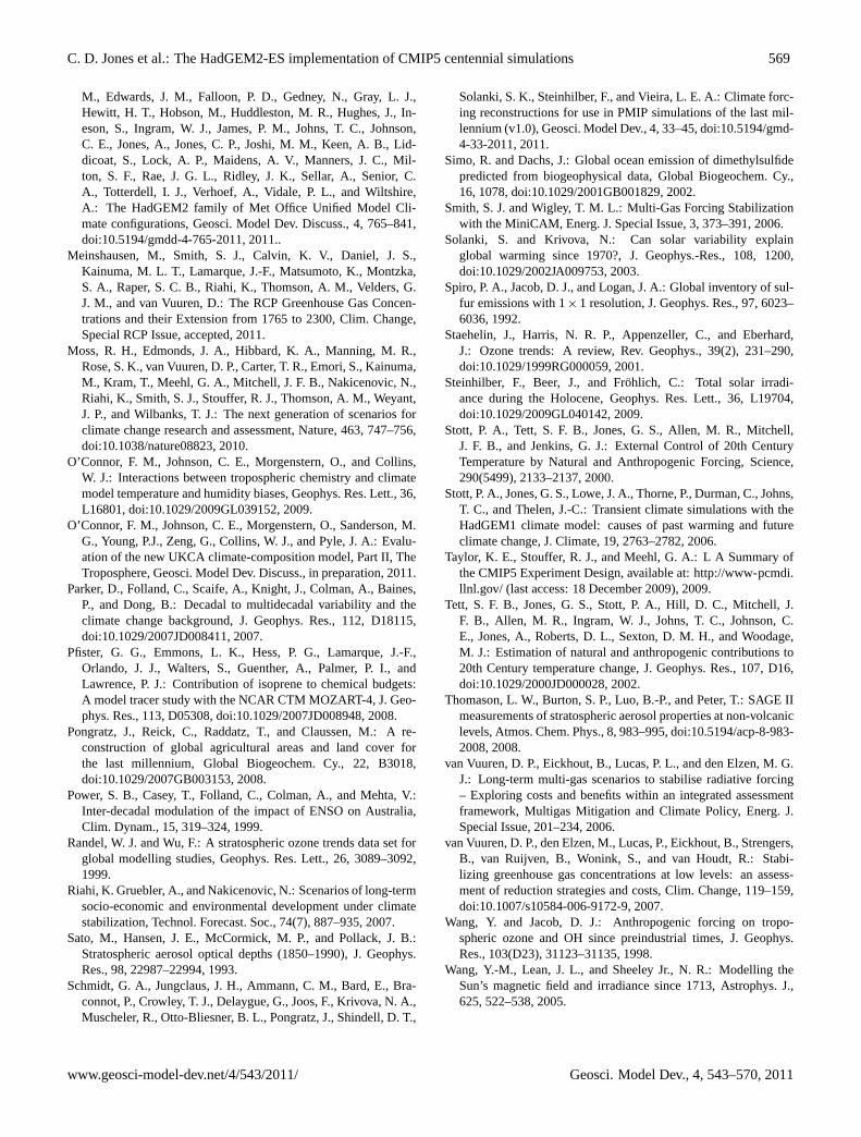
C. D. Jones et al.: The HadGEM2-ES implementation of CMIP5 centennial simulations 569
M., Edwards, J. M., Falloon, P. D., Gedney, N., Gray, L. J.,Hewitt, H. T., Hobson, M., Huddleston, M. R., Hughes, J., In-eson, S., Ingram, W. J., James, P. M., Johns, T. C., Johnson,C. E., Jones, A., Jones, C. P., Joshi, M. M., Keen, A. B., Lid-dicoat, S., Lock, A. P., Maidens, A. V., Manners, J. C., Mil-ton, S. F., Rae, J. G. L., Ridley, J. K., Sellar, A., Senior, C.A., Totterdell, I. J., Verhoef, A., Vidale, P. L., and Wiltshire,A.: The HadGEM2 family of Met Office Unified Model Cli-mate configurations, Geosci. Model Dev. Discuss., 4, 765–841,doi:10.5194/gmdd-4-765-2011, 2011..
Meinshausen, M., Smith, S. J., Calvin, K. V., Daniel, J. S.,Kainuma, M. L. T., Lamarque, J.-F., Matsumoto, K., Montzka,S. A., Raper, S. C. B., Riahi, K., Thomson, A. M., Velders, G.J. M., and van Vuuren, D.: The RCP Greenhouse Gas Concen-trations and their Extension from 1765 to 2300, Clim. Change,Special RCP Issue, accepted, 2011.
Moss, R. H., Edmonds, J. A., Hibbard, K. A., Manning, M. R.,Rose, S. K., van Vuuren, D. P., Carter, T. R., Emori, S., Kainuma,M., Kram, T., Meehl, G. A., Mitchell, J. F. B., Nakicenovic, N.,Riahi, K., Smith, S. J., Stouffer, R. J., Thomson, A. M., Weyant,J. P., and Wilbanks, T. J.: The next generation of scenarios forclimate change research and assessment, Nature, 463, 747–756,doi:10.1038/nature08823, 2010.
O’Connor, F. M., Johnson, C. E., Morgenstern, O., and Collins,W. J.: Interactions between tropospheric chemistry and climatemodel temperature and humidity biases, Geophys. Res. Lett., 36,L16801,doi:10.1029/2009GL039152, 2009.
O’Connor, F. M., Johnson, C. E., Morgenstern, O., Sanderson, M.G., Young, P.J., Zeng, G., Collins, W. J., and Pyle, J. A.: Evalu-ation of the new UKCA climate-composition model, Part II, TheTroposphere, Geosci. Model Dev. Discuss., in preparation, 2011.
Parker, D., Folland, C., Scaife, A., Knight, J., Colman, A., Baines,P., and Dong, B.: Decadal to multidecadal variability and theclimate change background, J. Geophys. Res., 112, D18115,doi:10.1029/2007JD008411, 2007.
Pfister, G. G., Emmons, L. K., Hess, P. G., Lamarque, J.-F.,Orlando, J. J., Walters, S., Guenther, A., Palmer, P. I., andLawrence, P. J.: Contribution of isoprene to chemical budgets:A model tracer study with the NCAR CTM MOZART-4, J. Geo-phys. Res., 113, D05308,doi:10.1029/2007JD008948, 2008.
Pongratz, J., Reick, C., Raddatz, T., and Claussen, M.: A re-construction of global agricultural areas and land cover forthe last millennium, Global Biogeochem. Cy., 22, B3018,doi:10.1029/2007GB003153, 2008.
Power, S. B., Casey, T., Folland, C., Colman, A., and Mehta, V.:Inter-decadal modulation of the impact of ENSO on Australia,Clim. Dynam., 15, 319–324, 1999.
Randel, W. J. and Wu, F.: A stratospheric ozone trends data set forglobal modelling studies, Geophys. Res. Lett., 26, 3089–3092,1999.
Riahi, K. Gruebler, A., and Nakicenovic, N.: Scenarios of long-termsocio-economic and environmental development under climatestabilization, Technol. Forecast. Soc., 74(7), 887–935, 2007.
Sato, M., Hansen, J. E., McCormick, M. P., and Pollack, J. B.:Stratospheric aerosol optical depths (1850–1990), J. Geophys.Res., 98, 22987–22994, 1993.
Schmidt, G. A., Jungclaus, J. H., Ammann, C. M., Bard, E., Bra-connot, P., Crowley, T. J., Delaygue, G., Joos, F., Krivova, N. A.,Muscheler, R., Otto-Bliesner, B. L., Pongratz, J., Shindell, D. T.,
Solanki, S. K., Steinhilber, F., and Vieira, L. E. A.: Climate forc-ing reconstructions for use in PMIP simulations of the last mil-lennium (v1.0), Geosci. Model Dev., 4, 33–45,doi:10.5194/gmd-4-33-2011, 2011.
Simo, R. and Dachs, J.: Global ocean emission of dimethylsulfidepredicted from biogeophysical data, Global Biogeochem. Cy.,16, 1078,doi:10.1029/2001GB001829, 2002.
Smith, S. J. and Wigley, T. M. L.: Multi-Gas Forcing Stabilizationwith the MiniCAM, Energ. J. Special Issue, 3, 373–391, 2006.
Solanki, S. and Krivova, N.: Can solar variability explainglobal warming since 1970?, J. Geophys.-Res., 108, 1200,doi:10.1029/2002JA009753, 2003.
Spiro, P. A., Jacob, D. J., and Logan, J. A.: Global inventory of sul-fur emissions with 1× 1 resolution, J. Geophys. Res., 97, 6023–6036, 1992.
Staehelin, J., Harris, N. R. P., Appenzeller, C., and Eberhard,J.: Ozone trends: A review, Rev. Geophys., 39(2), 231–290,doi:10.1029/1999RG000059, 2001.
Steinhilber, F., Beer, J., and Frohlich, C.: Total solar irradi-ance during the Holocene, Geophys. Res. Lett., 36, L19704,doi:10.1029/2009GL040142, 2009.
Stott, P. A., Tett, S. F. B., Jones, G. S., Allen, M. R., Mitchell,J. F. B., and Jenkins, G. J.: External Control of 20th CenturyTemperature by Natural and Anthropogenic Forcing, Science,290(5499), 2133–2137, 2000.
Stott, P. A., Jones, G. S., Lowe, J. A., Thorne, P., Durman, C., Johns,T. C., and Thelen, J.-C.: Transient climate simulations with theHadGEM1 climate model: causes of past warming and futureclimate change, J. Climate, 19, 2763–2782, 2006.
Taylor, K. E., Stouffer, R. J., and Meehl, G. A.: L A Summary ofthe CMIP5 Experiment Design, available at:http://www-pcmdi.llnl.gov/ (last access: 18 December 2009), 2009.
Tett, S. F. B., Jones, G. S., Stott, P. A., Hill, D. C., Mitchell, J.F. B., Allen, M. R., Ingram, W. J., Johns, T. C., Johnson, C.E., Jones, A., Roberts, D. L., Sexton, D. M. H., and Woodage,M. J.: Estimation of natural and anthropogenic contributions to20th Century temperature change, J. Geophys. Res., 107, D16,doi:10.1029/2000JD000028, 2002.
Thomason, L. W., Burton, S. P., Luo, B.-P., and Peter, T.: SAGE IImeasurements of stratospheric aerosol properties at non-volcaniclevels, Atmos. Chem. Phys., 8, 983–995,doi:10.5194/acp-8-983-2008, 2008.
van Vuuren, D. P., Eickhout, B., Lucas, P. L., and den Elzen, M. G.J.: Long-term multi-gas scenarios to stabilise radiative forcing– Exploring costs and benefits within an integrated assessmentframework, Multigas Mitigation and Climate Policy, Energ. J.Special Issue, 201–234, 2006.
van Vuuren, D. P., den Elzen, M., Lucas, P., Eickhout, B., Strengers,B., van Ruijven, B., Wonink, S., and van Houdt, R.: Stabi-lizing greenhouse gas concentrations at low levels: an assess-ment of reduction strategies and costs, Clim. Change, 119–159,doi:10.1007/s10584-006-9172-9, 2007.
Wang, Y. and Jacob, D. J.: Anthropogenic forcing on tropo-spheric ozone and OH since preindustrial times, J. Geophys.Res., 103(D23), 31123–31135, 1998.
Wang, Y.-M., Lean, J. L., and Sheeley Jr., N. R.: Modelling theSun’s magnetic field and irradiance since 1713, Astrophys. J.,625, 522–538, 2005.
www.geosci-model-dev.net/4/543/2011/ Geosci. Model Dev., 4, 543–570, 2011

570 C. D. Jones et al.: The HadGEM2-ES implementation of CMIP5 centennial simulations
Woodward, S.: Modelling the atmospheric life cycle and radiativeimpact of mineral dust in the Hadley Centre climate model. J.Geophys. Res., 106, D16, 18155–18166, 2001.
Woodward S.: Mineral Dust in HadGEM2, Met Office Hadley Cen-tre, Technical Note 87, 2011.
Yienger, J. and Levy II, H.: Empirical model of global soil-biogenicNOx emissions, J. Geophys. Res., 100(D6), 11447–11464, 1995.
Geosci. Model Dev., 4, 543–570, 2011 www.geosci-model-dev.net/4/543/2011/