1

INTRODUCTION

1.1 ELECTRON CONFIGURATION IN ATOMS

The periodic law is most commonly expressed in chemistry in the form of a periodic

table or chart. An important part of this table is shown in Table 1.1. The so-called

short-form periodic table, based on the Mendeleev table, with subsequent

emendations and additions, is still in widespread use. The elements in this table are

arranged in seven horizontal rows, called the periods, in order of increasing atomic

weight, and in 18 vertical columns, called the groups. The first period, containing two

elements, H and He, and the next two periods, each containing eight elements, are

called the short periods. The remaining periods, called the long periods, contain 18

elements, as in periods 4 and 5, or 32 elements, as in period 6. The long period 7

includes the actinoid series which has been filled in by the synthesis of radioactive

nuclei through element 103, lawrencium (Lr). Heavier transuranium elements (atomic

numbers 104 to 118) have also been synthesized.

The rules of placing electrons within shells are known as the Aufbau principle [1].

These rules are: (i) a maximum of two electrons are put into orbitals in the order of

increasing orbital energy; (ii) the lowest-energy orbitals are filled before electrons are

placed in higher-energy orbitals. The Aufbau principle works very well for the first

18 elements, then decreasingly well for the following 100 elements.

The modern form of the Aufbau principle describes an order of atomic orbital

energies given by Madelung's rule [2] (or Klechkowski's rule [3]). This rule is: (i)

The

Han

dboo

k on

Opt

ical

Con

stan

ts o

f M

etal

s D

ownl

oade

d fr

om w

ww

.wor

ldsc

ient

ific

.com

by U

NIV

ER

SIT

Y O

F O

TT

AW

A o

n 06

/01/

13. F

or p

erso

nal u

se o

nly.

Introduction

2

Table 1.1 Periodic table.

* Elements in the gray boxes are of interest in this book.

orbitals are filled in the order of increasing n+l; (ii) when two orbitals have the same

value of n+l, they are filled in order of increasing n, where n is the principal quantum

number (n = 1 (K), 2 (L), 3 (M), 4 (N), 5 (O), 6 (P), 7 (Q), …) and l is the azimuthal

quantum number (l = 0 (s), 1 (p), 2 (d), 3 (f), 4 (g), 5 (h), 6 (i), …). The above rule

gives the following order for filling the orbitals:

1s, 2s, 2p, 3s, 3p, 4s, 3d, 4p, 5s, 4d, 5p, 6s, 4f, 5d, 6p, 7s, 5f, 6d and 7p

As shown in Table 1.2, there are several exceptions to Madelung's rule among the

heavier elements (Nb, Mo, Tc, Ru, Rh, Pd, Ag, La, Ce, etc.).

Table 1.2 Electron configuration in atoms.

K L M N O P Q

1s 2s 2p 3s 3p 3d 4s 4p 4d 4f 5s 5p 5d 5f 5g 6s 6p 6d 6f 6g 6h 7s

1 H 1

2 He 2

3 Li 2 1

4 Be 2 2

5 B 2 2 1

6 C 2 2 2

7 N 2 2 3

8 O 2 2 4

9 F 2 2 5

10 Ne 2 2 6

11 Na 1

12 Mg 2

13 Al 2 1

14 Si Ne shell 2 2

The

Han

dboo

k on

Opt

ical

Con

stan

ts o

f M

etal

s D

ownl

oade

d fr

om w

ww

.wor

ldsc

ient

ific

.com

by U

NIV

ER

SIT

Y O

F O

TT

AW

A o

n 06

/01/

13. F

or p

erso

nal u

se o

nly.

1.1 Electron Configuration in Atoms

3

15 P 2 3

16 S 2 4

17 Cl 2 5

18 Ar 2 6

19 K 1

20 Ca 2

21 Sc 1 2

22 Ti 2 2

23 V 3 2

24 Cr 5 1

25 Mn 5 2

26 Fe 6 2

27 Co Ar shell

7 2

28 Ni 8 2

29 Cu 10 1

30 Zn 10 2

31 Ga 10 2 1

32 Ge 10 2 2

33 As 10 2 3

34 Se 10 2 4

35 Br 10 2 5

36 Kr 10 2 6

37 Rb 1

38 Sr 2

39 Y 1 2

40 Zr 2 2

41 Nb 4 1

42 Mo 5 1

43 Tc 6 1

44 Ru 7 1

45 Rh Kr shell

8 1

46 Pd 10 0

47 Ag 10 1

48 Cd 10 2

49 In 10 2 1

50 Sn 10 2 2

51 Sb 10 2 3

52 Te 10 2 4

53 In 10 2 5

54 Xe 10 2 6

55 Cs 1

56 Ba 2

57 La 1 2

58 Ce 1 1 2

59 Pr 3 0 2

60 Nd 4 0 2

61 Pm 5 0 2

62 Sm 6 0 2

63 Eu 7 0 2

64 Gd 7 1 2

65 Tb 9 0 2

The

Han

dboo

k on

Opt

ical

Con

stan

ts o

f M

etal

s D

ownl

oade

d fr

om w

ww

.wor

ldsc

ient

ific

.com

by U

NIV

ER

SIT

Y O

F O

TT

AW

A o

n 06

/01/

13. F

or p

erso

nal u

se o

nly.

Introduction

4

66 Dy 10 0 2

67 Ho 11 0 2

68 Er 12 0 2

69 Tm 13 0 2

70 Yb Xe shell

14 0 2

71 Lu 14 1 2

72 Hf 14 2 2

73 Ta 14 3 2

74 W 14 4 2

75 Re 14 5 2

76 Os 14 6 2

77 Ir 14 7 2

78 Pt 14 9 1

79 Au 14 10 1

80 Hg 14 10 2

81 Tl 14 10 2 1

82 Pb 14 10 2 2

83 Bi 14 10 2 3

84 Po 14 10 2 4

85 At 14 10 2 5

86 Rn 14 10 2 6

87 Fr 1

88 Ra 2

89 Ac 1 2

90 Th 2 2

91 Pa 2 1 2

92 U 3 1 2

93 Np 4 1 2

94 Pu 6 0 2

95 Am Rn shell 7 0 2

96 Cm 7 1 2

97 Bk 9 0 2

98 Cf 10 0 2

99 Es 11 0 2

100 Fm 12 0 2

101 Md 13 0 2

102 No 14 0 2

103 Lr 14 1 2

1.2 CRYSTAL STRUCTURE

1.2.1 Metal and Semimetal Elements

(a) Metallic bond

There are two condensed states of matter, namely, the solid and liquid states. In the

liquid state, the spatial order is almost nonexistent whereas in the solid state of most

materials, the regularity of atomic pattern or spatial order extends over distances

The

Han

dboo

k on

Opt

ical

Con

stan

ts o

f M

etal

s D

ownl

oade

d fr

om w

ww

.wor

ldsc

ient

ific

.com

by U

NIV

ER

SIT

Y O

F O

TT

AW

A o

n 06

/01/

13. F

or p

erso

nal u

se o

nly.

1.2 Crystal Structure

5

hundreds or thousands of times the diameter of the atoms. Most of the physical

properties of such crystals owe their existence to this long-range order. At room

temperature, Hg is in a liquid state with a melting point at Tm = −38.842°C while Tm

of Ga is 29.78°C.

Atoms of different elements have different spatial distributions of outer electrons

and they are accommodated in a solid so that the energy, subject to the given quantum

rules, is a minimum. It is possible to classify atomic bonds into five groups: (i)

metallic, (ii) covalent, (iii) ionic, (iv) van der Waals and (v) hydrogen. Table 1.3

presents a few values of binding energy of each atomic bond. The binding energy is

approximately equal to the latent heat of vaporization.

In metals, positively charged ion cores are held together by their attraction to the

free electrons which form a cloud between them. The free electrons are not localized

on an atomic scale and give rise to high electrical and thermal conductivity to the

metal. There are more allowed quantum states than the number of electrons and in

many ways, the metallic bond is like an unsaturated covalent bond. Consequently, the

metallic bond is much less directional than the covalent bond which explains the

structure’s packing efficiency. Therefore, many metals are close-packed. The lack of

quantum restriction on the electrons also removes any restriction on the kind of

neighbor a metallic atom can have. Thus, metals have the characteristic of forming

alloys.

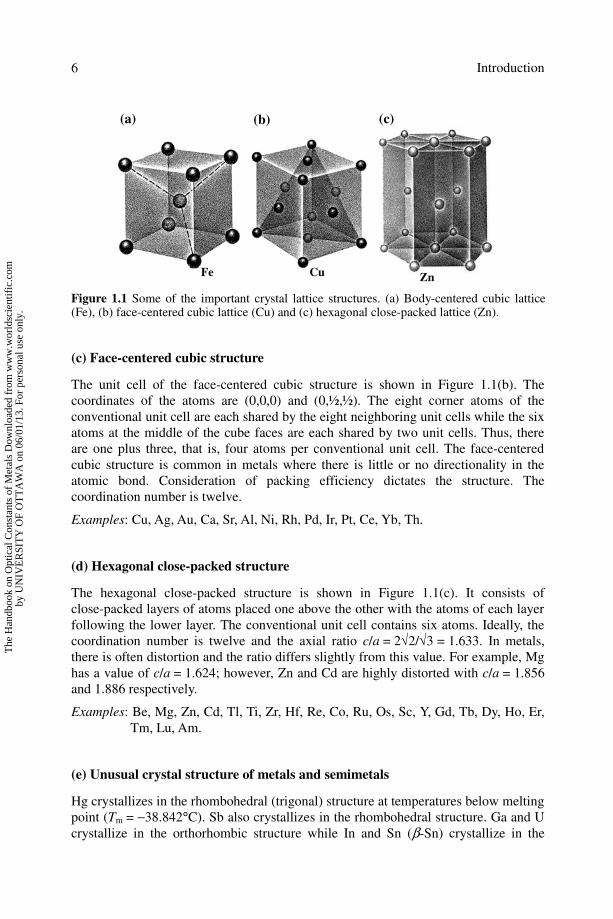
(b) Body-centered cubic structure

The simplest crystal structure found among the elements is called body-centered

cubic. The conventional unit cell is shown in Figure 1.1(a) where the three axes of the

primitive unit cell are marked by dashed lines. The conventional unit cell contains

two atoms. This can readily be seen since the eight corner atoms are each shaded by

eight neighboring cells whereas the central atom is uniquely associated with the cell

drawn. The coordinates of the atoms in the conventional cell are (0,0,0) and (½,½,½).

The coordination number is eight. Consideration of directionality of bond prevents

the structure from being closed-packed. Examples: Li, Na, K, Rb, Cs, Ba, V, Nb, Ta, Cr, Mo, W, Fe, Eu.

Table 1.3 Approximate binding energies of solids (in kJ/mol).

Bond Material

Metallic Al

327 Cu 336

Fe 413

Covalent C (diamond)

711

Ionic NaCl 765

KCl 688

AgCl 861

van der Waals Ar 7.7

CH4 10.0

Hydrogen H2O 50

The

Han

dboo

k on

Opt

ical

Con

stan

ts o

f M

etal

s D

ownl

oade

d fr

om w

ww

.wor

ldsc

ient

ific

.com

by U

NIV

ER

SIT

Y O

F O

TT

AW

A o

n 06

/01/

13. F

or p

erso

nal u

se o

nly.

Introduction

6

(a) (b) (c)

Fe Cu Zn

Figure 1.1 Some of the important crystal lattice structures. (a) Body-centered cubic lattice (Fe), (b) face-centered cubic lattice (Cu) and (c) hexagonal close-packed lattice (Zn).

(c) Face-centered cubic structure

The unit cell of the face-centered cubic structure is shown in Figure 1.1(b). The

coordinates of the atoms are (0,0,0) and (0,½,½). The eight corner atoms of the

conventional unit cell are each shared by the eight neighboring unit cells while the six

atoms at the middle of the cube faces are each shared by two unit cells. Thus, there

are one plus three, that is, four atoms per conventional unit cell. The face-centered

cubic structure is common in metals where there is little or no directionality in the

atomic bond. Consideration of packing efficiency dictates the structure. The

coordination number is twelve. Examples: Cu, Ag, Au, Ca, Sr, Al, Ni, Rh, Pd, Ir, Pt, Ce, Yb, Th.

(d) Hexagonal close-packed structure

The hexagonal close-packed structure is shown in Figure 1.1(c). It consists of

close-packed layers of atoms placed one above the other with the atoms of each layer

following the lower layer. The conventional unit cell contains six atoms. Ideally, the

coordination number is twelve and the axial ratio c/a = 2√2/√3 = 1.633. In metals,

there is often distortion and the ratio differs slightly from this value. For example, Mg

has a value of c/a = 1.624; however, Zn and Cd are highly distorted with c/a = 1.856

and 1.886 respectively. Examples: Be, Mg, Zn, Cd, Tl, Ti, Zr, Hf, Re, Co, Ru, Os, Sc, Y, Gd, Tb, Dy, Ho, Er,

Tm, Lu, Am.

(e) Unusual crystal structure of metals and semimetals

Hg crystallizes in the rhombohedral (trigonal) structure at temperatures below melting

point (Tm = −38.842°C). Sb also crystallizes in the rhombohedral structure. Ga and U

crystallize in the orthorhombic structure while In and Sn (β-Sn) crystallize in the

The

Han

dboo

k on

Opt

ical

Con

stan

ts o

f M

etal

s D

ownl

oade

d fr

om w

ww

.wor

ldsc

ient

ific

.com

by U

NIV

ER

SIT

Y O

F O

TT

AW

A o

n 06

/01/

13. F

or p

erso

nal u

se o

nly.

1.2 Crystal Structure

7

Ti+

N−−−−

tetragonal structure. Graphite (C) is a layered material. In each layer, the carbon

atoms are arranged in the hexagonal lattice with a separation of 0.142 nm, and the

distance between planes is 0.335 nm. La, Pr and Nd can crystallize in the double

hexagonal close-packed structure with a layered structure like ABAC… . Sm

crystallizes in the complex hexagonal close-packed structure with nine repeating

layers like ABCBCACAB… . Mn has a distorted body-centered cubic structure with

unit cell containing Mn atoms in four different environments.

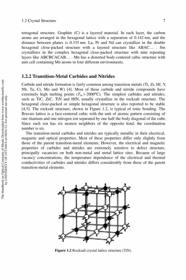
1.2.2 Transition-Metal Carbides and Nitrides

Carbide and nitride formation is fairly common among transition metals (Ti, Zr, Hf, V,

Nb, Ta, Cr, Mo and W) [4]. Most of these carbide and nitride compounds have

extremely high melting points (Tm > 2000°C). The simplest carbides and nitrides,

such as TiC, ZrC, TiN and HfN, usually crystallize in the rocksalt structure. The

hexagonal close-packed or simple hexagonal structure is also reported to be stable

[4,5]. The rocksalt structure, shown in Figure 1.2, is typical of ionic bonding. The

Bravais lattice is a face-centered cubic with the unit of atomic pattern consisting of

one titanium and one nitrogen ion separated by one half the body diagonal of the cube.

Since each ion has six nearest neighbors of the opposite kind, the coordination

number is six.

The transition-metal carbides and nitrides are typically metallic in their electrical,

magnetic and optical properties. Most of these properties differ only slightly from

those of the parent transition-metal elements. However, the electrical and magnetic

properties of carbides and nitrides are extremely sensitive to defect structure,

principally vacancies on both non-metal and metal lattice sites. Because of large

vacancy concentrations, the temperature dependence of the electrical and thermal

conductivities of carbides and nitrides differs considerably from those of the parent

transition-metal elements.

Figure 1.2 Rocksalt crystal lattice structure (TiN).

The

Han

dboo

k on

Opt

ical

Con

stan

ts o

f M

etal

s D

ownl

oade

d fr

om w

ww

.wor

ldsc

ient

ific

.com

by U

NIV

ER

SIT

Y O

F O

TT

AW

A o

n 06

/01/

13. F

or p

erso

nal u

se o

nly.

Introduction

8

Si

Co

Si V

(b) (a)

1.2.3 Metallic Silicides

From electrical and optical viewpoints, metal silicides can be classified into two

groups: metallic and semiconducting silicides. Therefore, the chemical bonds in metal

silicides range from conductive metal-like structures to covalent or ionic. Metallic

silicides demonstrate a variety of crystalline structures, namely, cubic (CoSi2, NiSi2,

etc.), tetragonal (γ-FeSi2, Ru2Si3, etc.), hexagonal (VSi2, NbSi2, etc.), rhombohedral

(Cu3Si), orthorhombic (TiSi2, HfSi2, etc.) and monoclinic structures (Rh4Si5, Pd5Si,

etc.) [6].

Figures 1.3(a) and 1.3(b) show the crystal structures of VSi2 and CoSi2 respectively.

VSi2 crystallizes in the hexagonal structure (space group = P6222). The measured

lattice constants of VSi2 are a = 0.457230 nm and c = 0.63730 nm with c/a = 1.3938

[6]. Pd2Si also crystallizes in the hexagonal lattice with the space group of mP 26 ;

however, its lattice-constant ratio is smaller than unity, c/a = 0.5347 with a = 0.6493

nm and c = 0.3472 nm [6].

CoSi2 crystallizes in the cubic structure (space group = Fm3m). Its crystal structure

is the same as that of fluorite, CaF2. As shown in Figure 1.3(b), the fluorite structure

is a type of ionic crystal structure in which the cations have an expanded

face-centered cubic arrangement with the anions occupying both types of tetrahedral

hole. The cations have a coordination number of eight and the anions have a

coordination number of four.

1.2.4 High-Tc Superconductors

(a) YBa2Cu3O7−−−−δδδδ

Only a few oxides with critical temperatures Tc above the boiling point of liquid

helium (4.2 K) were known up to 1986. Such low-Tc superconductors did not exceed

19 K [7]. The first superconducting compounds with Tc above the boiling point of

liquid nitrogen was discovered as a mixed copper oxide representative of the system

Y−Ba−Cu−O at ambient pressure in 1987 and this marked the beginning of the

worldwide high-Tc superconductor research [7].

Figure 1.3 Crystal structure of metallic silicide. (a) VSi2 and (b) CoSi2.

The

Han

dboo

k on

Opt

ical

Con

stan

ts o

f M

etal

s D

ownl

oade

d fr

om w

ww

.wor

ldsc

ient

ific

.com

by U

NIV

ER

SIT

Y O

F O

TT

AW

A o

n 06

/01/

13. F

or p

erso

nal u

se o

nly.

1.3 Dielectric Function: Tensor Representation

9

The crystal structures of YBa2Cu3O7−δ with (a) δ = 1 (YBa2Cu3O6) and (b) δ = 0

(YBa2Cu3O7) are schematically shown in Figure 1.4. The high-Tc compound

YBa2Cu3O7−δ crystallizes in the orthorhombic space group of Pmmm with Tc ∼ 90 K

for 0 ≤ δ ≤ 0.2. The superconducting properties are known to depend on the oxygen

content. For δ = 0, the unit cell contains one Cu atom in the oxidation state Cu3+

and

two atoms in the oxidation state Cu2+

. The latter Cu atoms are coordinated by five O

atoms and form a square-pyramidal coordination sphere while the remaining Cu atom

shows a fourfold, nearly square-planar coordination. These rectangles are connected

via vertices forming chains along the b-axis. The pyramids are also connected via

vertices forming a two-dimensional arrangement within the ab-plane. The O−Cu−O

angles within the layers are smaller than 2π, thus distorting the plane character of the

layers [7].

The non-superconducting YBa2Cu3O7−δ (an antiferromagnetic insulator) phase with

0.5 ≤ δ ≤ 0.1 crystallizes in a tetragonal unit cell with the space group of P4/mmm. It

should be noted that for δ = 1, only linear coordinated Cu(I) atoms are present.

(b) Bi2Sr2CaCu2O8

The high-Tc compound Bi2Sr2CaCu2O8 crystallizes in the orthorhombic space group

of Fmmm with Tc = 96 K [8]. In Figure 1.5, the structure element carrying the mobile

charges is a stack of two CuO2 monolayers which are separated by an intermediate

monolayer of alkaline earth element Ca. These stacks of CuO2/Ca are sandwiched

between insulating blocks consisting of two monolayers of Bi-oxide and two

monolayers of Sr-oxide. These blocks can act as electrically active charge-reservoirs

for hole or electron donation to the Cu−O layers.

(c) MgB2

In spite of the fact that MgB2 has been known since the early 1950s, it was unknown

until 2001 that it is a superconductor [9]. Reported Tc value for MgB2 is 40.2 K [10].

MgB2 crystallizes in the simple hexagonal AlB2-type structure and contains

graphite-type B layers that are separated by hexagonal close-packed layers of Mg, as

schematically shown in Figure 1.6. Although MgB2 does not have an attractively high

transition temperature, there is an advantage of strongly linked grains that enable high

current flow across the grain boundaries of bulk polycrystalline MgB2.

1.3 DIELECTRIC FUNCTION: TENSOR

REPRESENTATION

In an anisotropic medium, the polarization and induced current generally lie in a

direction different from that of the electric field. In that case, it is possible, e.g., to

induce a longitudinal current with a purely transverse electric field. This situation can

be treated by representing the dielectric function as a tenor [11].

The

Han

dboo

k on

Opt

ical

Con

stan

ts o

f M

etal

s D

ownl

oade

d fr

om w

ww

.wor

ldsc

ient

ific

.com

by U

NIV

ER

SIT

Y O

F O

TT

AW

A o

n 06

/01/

13. F

or p

erso

nal u

se o

nly.

Introduction

10

Figure 1.4 Crystal structures of YBa2Cu3O7−δ with (a) δ = 1 (YBa2Cu3O6) and (b) δ = 0 (YBa2Cu3O7).

Figure 1.5 Crystal structure of Bi2Sr2CaCu2O8.

Figure 1.6 Crystal structure of MgB2.

The

Han

dboo

k on

Opt

ical

Con

stan

ts o

f M

etal

s D

ownl

oade

d fr

om w

ww

.wor

ldsc

ient

ific

.com

by U

NIV

ER

SIT

Y O

F O

TT

AW

A o

n 06

/01/

13. F

or p

erso

nal u

se o

nly.

1.4 Optical Dispersion Relations

11

We consider the polarization, that is, the electric moment per unit volume or the

polarization charge per unit area taken perpendicular to the direction of polarization.

The relationship of the ith spatial component of the polarization is expressed in terms

of the electric field components by a power series of the form

∑ ∑ ⋅⋅⋅++=j kj

kjijkjiji EEEP,

γχ (1.1)

With the advent of lasers, it is now quite common to observe nonlinear optical

phenomena. However, the concern in this book is only with linear optics and only

linear terms will be retained in expressions such as Equation (1.1).

The optical-related vectors can now be connected by the relation

PED π4+= (1.2)

where D and E are the dielectric displacement and field strength respectively and ε0

(the permittivity of a vacuum) is a scalar constant with the numerical value of

8.854 × 10−12

F/m. In many substances, the polarization is directly proportional to the

field strength E and thus, we write

EP χ= (1.3)

Hence,

( ) EED επχ =+= 41 (1.4)

where χ is the dielectric susceptibility and ε is usually called the dielectric constant or

dielectric function.

The dielectric susceptibility is a symmetric second-rank tensor. We have, then,

instead of Equation (1.4)

( ) ∑∑ =+=j

jijj

jijijiEED επχδ 4 (1.5)

where δij is the Kronecker delta. The dielectric or optical properties of a crystal may

thus be characterized by the magnitudes and directions of the three principal dielectric

constants, dielectric permittivities or dielectric susceptibilities. These magnitudes and

directions will, in principle, depend on the frequency of the electric field but they

must always, of course, conform to any restrictions imposed by crystal symmetry [11].

Table 1.4 summarizes the effect of crystal symmetry on dielectric properties

represented by a symmetric second-rank tensor.

1.4 OPTICAL DISPERSION RELATIONS

The complex dielectric function

)()()( 21 EiEE εεε += (1.6)

can describe the optical properties of the medium at all photon energies E. The

The

Han

dboo

k on

Opt

ical

Con

stan

ts o

f M

etal

s D

ownl

oade

d fr

om w

ww

.wor

ldsc

ient

ific

.com

by U

NIV

ER

SIT

Y O

F O

TT

AW

A o

n 06

/01/

13. F

or p

erso

nal u

se o

nly.

Introduction

12

Table 1.4 Tensor form of ε for metals, semimetals and metallic compounds of certain crystal classes.

Crystal class Metal, semimetal and metallic compound Tensor form

Cubic

Li, Ba, V, Cr, Mn, Fe, Eu, TiC, ZrN, CoSi2, NiSi2, etc.

11

11

11

00

00

00

εε

ε

Hexagonal Rhombohedral

(Trigonal) Tetragonal

In, Be, Zn, In, Ti, β-Sn, Sb, Re, Co, Sc, Am, VSi2, TaSi2, YBa2Cu3O6, Bi2Sr2CaCu2O8, MgB2, etc.

33

11

11

00

00

00

εε

ε

Orthorhombic Ga, α-U, TiSi2, HfSi2 and YBa2Cu3O7

33

22

11

00

00

00

εε

ε

complex refractive index n*(E) is obtained from

[ ] [ ] 2/1

21

2/1)()()()()()(* EiEEEikEnEn εεε +==+= (1.7)

where n(E) is the ordinary or real refractive index and k(E) is the extinction

coefficient. From Equation (1.7), it follows that

22

1 )()()( EkEnE −=ε (1.8a)

)()(2)(2 EkEnE =ε (1.8b)

and

[ ] 2/1

1

2/122

21

2

)()()()(

++=

EEEEn

εεε (1.9a)

[ ] 2/1

1

2/122

21

2

)()()()(

−+=

EEEEk

εεε (1.9b)

The Kramers−Kronig relations can also link n(E) and k(E) in the manner

∫∞

−+=

022

''

)'('21)( dE

EE

EkEEn

π (1.10a)

The

Han

dboo

k on

Opt

ical

Con

stan

ts o

f M

etal

s D

ownl

oade

d fr

om w

ww

.wor

ldsc

ient

ific

.com

by U

NIV

ER

SIT

Y O

F O

TT

AW

A o

n 06

/01/

13. F

or p

erso

nal u

se o

nly.

1.5 Optical Sum Rules

13

∫∞

−−

−=0 22

''

1)'(2)( dE

EE

EnEEk

π (1.10b)

The absorption coefficient α(E) and normal-incidence reflectivity R(E) can be

written as

)(4

)( EkEλπ

α = (1.11)

[ ]

[ ] 22

22

)(1)(

)(1)()(

EkEn

EkEnER

++

+−= (1.12)

where λ is the wavelength of light in vacuum.

1.5 OPTICAL SUM RULES

1.5.1 Inertial Sum Rule

The development of synchrotron radiation sources and advances in infrared, x-ray and

electron-energy-loss spectroscopy, as well as improvements in sample preparation,

have vastly extended the number and range of reliable optical measurements.

Moreover, advances in the theory have provided various optical sum rules [12,13] by

which the self-consistency of optical data can be checked.

The inertial sum rule

[ ]∫∞

=−0

01)( dEEn (1.13)

states that the average value of the refractive index is unity. This rule is a direct

consequence of causality and the law of inertia; it must be satisfied if n(E) has been

calculated from a physically acceptable k(E) by the Kramers−Kronig transformation.

1.5.2 dc-Conductivity Sum Rule

A second consequence of causality and the law of inertia is the dc-conductivity sum

rule

[ ]∫∞

−=−0

21 )0(21)( σdEE πε (1.14)

where σ(0) is the dc conductivity. The only net contribution to this integral is made

by the dispersion associated with the conduction electrons. This rule provides a test of

the conduction-electron spectrum (see Section 1.6.1).

The

Han

dboo

k on

Opt

ical

Con

stan

ts o

f M

etal

s D

ownl

oade

d fr

om w

ww

.wor

ldsc

ient

ific

.com

by U

NIV

ER

SIT

Y O

F O

TT

AW

A o

n 06

/01/

13. F

or p

erso

nal u

se o

nly.

Introduction

14

1.5.3 f-Sum Rule

The f-sum rule relates the number density of electrons to the dissipative or imaginary

part of the complex dielectric function, refractive index and energy-loss spectrum.

From the asymptotic behavior of ε(ω) at high frequencies

2

2p

1)(ω

ωωε −=∞→

(1.15)

together with the analyticity of ε(E) and ε(E)−1

, we obtain the following relations

2

p0

22

1)( πωωωωε =∫

∞d (1.16a)

and

2

p0

1

2

1)(Im πωωωεω −=∫

∞ − d (1.16b)

where ωp is the free-electron plasma frequency corresponding to the total electron

density of the system N

2/12

p

4

=

m

Neπω (1.17)

In Equation (1.17), e is the elementary charge and m is the electron effective mass.

Equation (1.16) is closely related to the Thomas−Reiche−Kuhn sum rule for an

atom in an initial state i.

∑ =j

ij Zf (1.18)

where the number of electrons in the atomic system is Z and the sum over j includes

continuum states. Here, a dimensionless quantity fij is known as the oscillator strength

and is defined by

2)(2

ijijij Mm

f ω�

= (1.19)

For a condensed rather than isolated atomic system, a sum rule analogous to

Equation (1.18) takes the form

Ndf =∫∞

0)( ωω (1.20)

where N is the electron density in the condensed material.

It is useful to define the effective number of electrons contributing to the optical

properties up to an energy E by the partial f sums.

∫=E

dEEEe

mEn

0222eff ')'('

2)( ε

π (1.21a)

∫=E

dEEkEe

mEn

022eff ')'(')(π

(1.21b)

[ ]∫−−=

E

dEEEe

mEn

0

1

22eff ')'(ln'2

)( επ

(1.21c)

The

Han

dboo

k on

Opt

ical

Con

stan

ts o

f M

etal

s D

ownl

oade

d fr

om w

ww

.wor

ldsc

ient

ific

.com

by U

NIV

ER

SIT

Y O

F O

TT

AW

A o

n 06

/01/

13. F

or p

erso

nal u

se o

nly.

1.5 Optical Sum Rules

15

10-3 10-2 10-1 100 101 102 103 1040

2

4

6

8

10

12

14

16

nef

f

E (eV)

3s23p1

K shell

L shell

Al

In the limit E → ∞, we can expect from Equation (1.21), neff(∞) = 13 for Al metal.

Figure 1.7 shows the calculated neff versus E plots for Al obtained by introducing

the experimental ε2(E) values listed in this book into Equation (1.21). neff rises to a

value near three, the free electron value. The absorptions of the conduction and core

electrons are well separated at the L edge (E ∼ 73 eV). The effective electron numbers,

eight and two, observed at E > 100 eV correspond to the L and K shell electrons

respectively. The K edge is observed to occur at ∼1200 eV.

An independent check on the dielectric function, as derived from optical

measurements, can be provided by comparison with the electron energy-loss spectra.

The electron-energy-loss function

2

2

2

1

21

Imεε

εε +

=

− (1.22)

involves both one-electron excitations and many body resonances such as excitons or

plasmons.

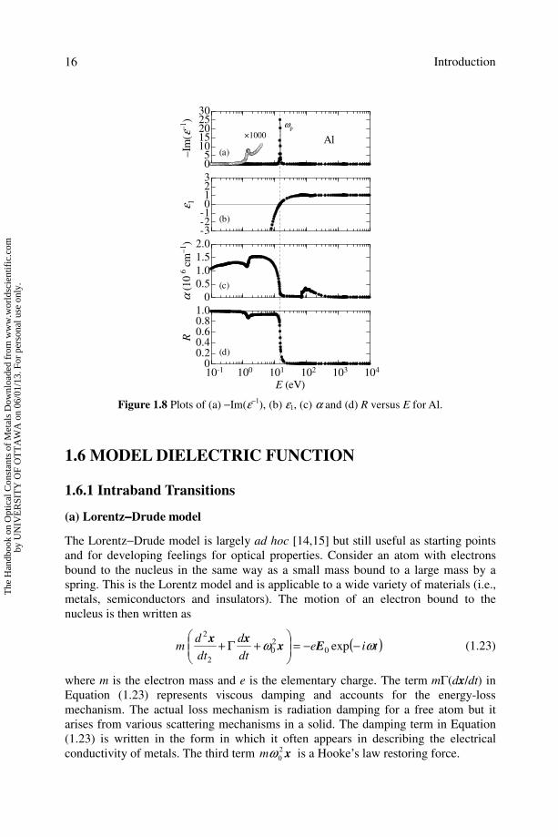
In Figure 1.8(a), we show the electron energy-loss spectrum of Al metal as

calculated from Equation (1.22) by introducing the experimental ε(E) data listed in

this book. The energy-loss spectrum in Figure 1.8(a) reveals the strong conduction

electron plasmon resonance at E = 15 eV. The plasmon frequency can also be

estimated from ε1(E) spectrum at which ε1 becomes zero (see Figure 1.8(b)). A weak

peak is also found in the energy-loss spectrum of Al at E ∼ 1.5 eV. This peak arises

from the interband transitions in Al.

The plasmon frequency ωp marks the transition between optically transparent and

optically reflecting regimes, as seen in Figures 1.8(c) and 1.8(d). Here, the optical

properties change very drastically and experimental errors may be quite large so that

even limited knowledge of the energy-loss function in the plasmon region is valuable

for verifying optical measurements.

Figure 1.7 neff versus E plot for Al. The plot is obtained by introducing experimental ε2(E) data listed in this book into Equation (1.21).

The

Han

dboo

k on

Opt

ical

Con

stan

ts o

f M

etal

s D

ownl

oade

d fr

om w

ww

.wor

ldsc

ient

ific

.com

by U

NIV

ER

SIT

Y O

F O

TT

AW

A o

n 06

/01/

13. F

or p

erso

nal u

se o

nly.

Introduction

16

05

1015202530

–Im

(ε–

1)

Al(a)

×1000

ωp

-3-2-10123

ε 1

(b)

0

0.5

1.0

1.5

2.0

α (

10

6 c

m–

1)

(c)

10-1 100 101 102 103 1040

0.20.40.60.81.0

E (eV)

R

(d)

Figure 1.8 Plots of (a) −Im(ε−1), (b) ε1, (c) α and (d) R versus E for Al.

1.6 MODEL DIELECTRIC FUNCTION

1.6.1 Intraband Transitions

(a) Lorentz−−−−Drude model

The Lorentz−Drude model is largely ad hoc [14,15] but still useful as starting points

and for developing feelings for optical properties. Consider an atom with electrons

bound to the nucleus in the same way as a small mass bound to a large mass by a

spring. This is the Lorentz model and is applicable to a wide variety of materials (i.e.,

metals, semiconductors and insulators). The motion of an electron bound to the

nucleus is then written as

( )tiedt

d

dt

dm ωω −−=

+Γ+ exp0

20

2

2

Exxx

(1.23)

where m is the electron mass and e is the elementary charge. The term mΓ(dx/dt) in

Equation (1.23) represents viscous damping and accounts for the energy-loss

mechanism. The actual loss mechanism is radiation damping for a free atom but it

arises from various scattering mechanisms in a solid. The damping term in Equation

(1.23) is written in the form in which it often appears in describing the electrical

conductivity of metals. The third term x2

0ωm is a Hooke’s law restoring force.

The

Han

dboo

k on

Opt

ical

Con

stan

ts o

f M

etal

s D

ownl

oade

d fr

om w

ww

.wor

ldsc

ient

ific

.com

by U

NIV

ER

SIT

Y O

F O

TT

AW

A o

n 06

/01/

13. F

or p

erso

nal u

se o

nly.

1.6 Model Dielectric Function

17

The solution to Equation (1.23) is

Γ−−

−=

ωωω im

e22

0

0 1ˆ

Ex (1.24)

The induced dipole moment is then given by

Γ−−=−=

ωωω im

ee

22

0

0

21

ˆˆE

xp (1.25)

We assume that the displacement x is sufficiently small that a linear relationship

exists between p̂ and E0, namely

0ˆˆ Ep α= (1.26)

where α̂ is the frequency-dependent atomic polarizability. From Equations (1.25)

and (1.26), we obtain the polarizability for a one-electron atom.

Γ−−=

ωωωα

im

e22

0

21

ˆ (1.27)

If there are N atoms per unit volume, the macroscopic polarization P is

EEpP χα =><=><= 0ˆNN (1.28)

From Equation (1.4), we obtain

Γ−−

+=+=

ωωωπ

ωεωεωεim

Nei

22

0

2

21

141)()()( (1.29)

Rationalizing Equation (1.29) gives

( )

Γ+−

−

+=

22222

0

22

0

2

1

41)(

ωωωωωπ

ωεm

Ne (1.30a)

( )

Γ+−

Γ

=

22222

0

2

2

4)(

ωωωωπ

ωεm

Ne (1.30b)

Since there is no restoring force for the conduction electrons, we rightly put

ω0 → 0. This provides the Drude expression widely used for metals and

semiconductors.

( ) ( )Γ+−=

Γ+

−=

iim

Ne

ωω

ω

ωωπ

ωε2

p

2

114

1)( (1.31)

Rationalizing Equation (1.31) also gives

The

Han

dboo

k on

Opt

ical

Con

stan

ts o

f M

etal

s D

ownl

oade

d fr

om w

ww

.wor

ldsc

ient

ific

.com

by U

NIV

ER

SIT

Y O

F O

TT

AW

A o

n 06

/01/

13. F

or p

erso

nal u

se o

nly.

Introduction

18

0 1 2 3 4-100

0

100

200

300

Lorentz

ε1

ε2

(×20)

E (eV)

ε

Drude

22

2

p

1 1)(Γ+

−=ω

ωωε (1.32a)

( )22

2p

2 )(Γ+

Γ=

ωω

ωωε (1.32b)

where ωp is the plasma frequency. It should be noted that the imaginary part of the

dielectric function ε2(ω) is proportional to Γ; hence, the same goes for the absorption

coefficient.

Figure 1.9 shows the spectral dependence of ε(E) calculated using Equations (1.29)

and (1.31) with ħω0 = 2.0 eV (Equation (1.29)) or ħω0 = 0 eV (Equation (1.31)),

ħωp = 1.0 eV and ħΓ = 0.1 eV. In the absence of an energy-loss mechanism, there is a

singularity at ω0. The maximum value of ε2 in Equation (1.30b) is

Γ

=0

2

p

2 (max)ω

ωε (1.33)

Equation (1.31) also predicts that ε1 (ε2) rapidly decreases (increases) with decreasing

ω. Such spectral features have been commonly observed in various metals.

(b) Optical constants and electrical conductivity

A free-carrier absorption process α(ω) is the annihilation of a photon with the

excitation of a carrier from a filled state below the Fermi energy EF to an empty state

above it. In a macroscopic view, the propagation of electromagnetic waves in an

absorbing medium is governed by a frequency-dependent conductivity σ(ω).

Therefore, the optical constants and electrical conductivity are not independent

properties.

From Equations (1.8), (1.11) and (1.32), we obtain

Figure 1.9 ε(E) calculated using the Lorentz and Drude models of Equations (1.29) and (1.31) respectively. The numerical values used are ħω0 = 2.0 (Equation (1.29)) or ħω0 = 0 eV (Equation (1.31)), ħωp = 1.0 eV and ħΓ = 0.1 eV.

The

Han

dboo

k on

Opt

ical

Con

stan

ts o

f M

etal

s D

ownl

oade

d fr

om w

ww

.wor

ldsc

ient

ific

.com

by U

NIV

ER

SIT

Y O

F O

TT

AW

A o

n 06

/01/

13. F

or p

erso

nal u

se o

nly.

1.6 Model Dielectric Function

19

( )22

2p

2

)()(

)()(

4)(

Γ+

Γ===

ωω

ωωε

ωω

ωλπ

ωαcncn

k (1.34)

where c is the speed of light. In the low-frequency limit ω → 0, the above equation

becomes

Γ=

Γ=

cmn

Ne

cn )0(

4

)0()0(

22p πω

α (1.35)

The low-field (dc) conductivity for free carriers is also given from a classical

transport theory by

m

NeNe

τµσ

2

)0( == (1.36)

where µ is the low-field mobility and τ is a phenomenological scattering time

introduced to account for the scattering of the electrons by phonons, impurities, etc.

Combining α(0) with σ(0) and equating Γ to τ−1, we obtain

)0()0(

4)0( σ

πα

cn= (1.37)

Thus, one can recognize a resemblance between the free-carrier absorption and

electron transport properties.

1.6.2 Interband Transitions

Metals are, in principle, similar to semiconductors. Their main distinctive feature is

the high density of conduction electrons in the metals. Thus, the basic theory of

interband transitions developed for semiconductors [16,17] can be used to discuss

interband absorption spectra in metals. Let us use the Lorentz model of Equation

(1.29) which gives exactly the same spectral features as a damped harmonic oscillator

used in semiconductors [16,17].

Using the Lorentz model, we obtain an expression for ε(ω) of metals over a wide

spectral range

∞+∑Γ−−

+Γ

−=1

0

22

0

0

22

2

p1)( ε

ωωωωω

ωεi

ii

i

i

C (1.38)

where ω0i, C0i and Γ0i are, respectively, the interband critical-point energy, strength

parameter and broadening parameter at each critical point i, and ε1∞ is the

nondispersive contribution to ε1, arising from any other higher-lying critical points

and/or core excitons.

The physical properties of the transition and noble metals are largely determined by

the outermost d electrons in the atoms. As this d shell is progressively filled through a

group of transition metals (Table 1.2), the physical properties vary drastically. The

noble metals follow right after the transition metals and have their d shell filled.

Although covering only energies below the Fermi level, the d bands in the noble

metals are still located in the region of band energies and they strongly influence the

band structure and the related physical properties.

The

Han

dboo

k on

Opt

ical

Con

stan

ts o

f M

etal

s D

ownl

oade

d fr

om w

ww

.wor

ldsc

ient

ific

.com

by U

NIV

ER

SIT

Y O

F O

TT

AW

A o

n 06

/01/

13. F

or p

erso

nal u

se o

nly.

Introduction

20

0 1 2 3 4 5 6 7 8 9 10-60

-40

-20

0

20

40

60

Cu

E (eV)

ε

ε1

ε2

We show the ε(E) spectrum of Cu in Figure 1.10. The real and imaginary ε(E)

values are plotted by the solid and open circles respectively. The solid lines represent

the calculated results using Equation (1.38) with ħωp = 7.5 eV, ħΓ = 0.08 eV,

ħω01 = 2.5 eV, C01 = 6.8 eV2, ħΓ01 = 0.8 eV, ħω02 = 3.3 eV, C02 = 14.4 eV

2, ħΓ02 = 1.6

eV, ħω03 = 5.0 eV, C03 = 67.2 eV2, ħΓ03 = 2.5 eV, ħω04 = 9.0 eV, C04 = 60.8 eV

2,

ħΓ04 = 3.5 eV and ε1∞ = −0.9. Individual contributions to ε2 of the intraband (Drude)

and interband transitions (i = 1 − 4) are also shown in Figure 1.11.

The experimental ε structure below ∼1 eV in Figures 1.10 and 1.11 corresponds to

the free-electron behavior typically observed in metals. The lowest interband

absorption starts to occur above 1.5 eV. In the non-noble (Cu) and noble metals (Ag,

Au), Cooper et al. [18] indicated that the sharp rise in ε2 at the lowest interband

absorption edge is due to the fact that the transitions are from a very flat lower band

to the Fermi surface and are not of the critical-point type. More strictly, these

transitions occur between occupied states in band 5 and unoccupied states in band 6

as these cross the Fermi surface (5 → 6 (EF)) at the L point in the Brillouin zone. Here,

the bands are numbered starting from the lowest band at a given k. Relatively poor

agreement between the Lorentz line shape and the experiment observed at ∼1.5 eV in

Figures 1.10 and 1.11 may reflect this fact.

The ħω03 = 5.0 eV structure in Figures 1.10 and 1.11 may correspond to transitions

from occupied states in band 4 to unoccupied states in band 6 at the X point [19]. The

broad structure at ħω04 = 9.0 eV is also thought to be due to transitions between

occupied states in band 5 to unoccupied states in bands 6−8 at the W point. The weak

peak at ħω02 = 3.3 eV may correspond to Fermi-level transitions along the ∆ direction

and/or at the Q point [19]. Figure 1.12 shows the locations of such interband

transitions in the k space of Cu.

Figure 1.10 Fitted result of the model dielectric function of Equation (1.38) to the experimental ε(E) data of Cu listed in this book.

The

Han

dboo

k on

Opt

ical

Con

stan

ts o

f M

etal

s D

ownl

oade

d fr

om w

ww

.wor

ldsc

ient

ific

.com

by U

NIV

ER

SIT

Y O

F O

TT

AW

A o

n 06

/01/

13. F

or p

erso

nal u

se o

nly.

References

21

0

5

10

15

20

Cu

ε 2

(a)

0 1 2 3 4 5 6 7 8 9 100

5

10

15

20

E (eV)

ε 2 ω01ω02

ω03

ω04

Drude

(b)

Figure 1.11 (a) Experimental and theoretical ε2(E) spectra of Cu at 300 K. The theoretical curve is obtained using Equation (1.38). (b) Individual contributions to ε2(E) of the free-carrier absorption (Drude) and the interband transitions (i = 1−4).

Figure 1.12 Energy band structure of Cu, including locations of several interband transitions.

References

[1] F. Weinhold and C. Landis, Valency and Bonding: A Natural Bond Orbital

Donor-Acceptor Perspective (Cambridge University Press, Cambridge, 2005).

[2] E. Madelung, Die mathematische Hilfsmittel des Physikers (Springer, Berlin,

1936).

[3] D. P. Wong, J. Chem. Educ. 56, 714 (1979).

[4] L. E. Toth, Transition Metal Carbides and Nitrides (Academic, New York,

1971).

[5] J.-E. Sundgren and H. T. G. Hentzell, J. Vac. Sci. Technol. A 4, 2259 (1986).

The

Han

dboo

k on

Opt

ical

Con

stan

ts o

f M

etal

s D

ownl

oade

d fr

om w

ww

.wor

ldsc

ient

ific

.com

by U

NIV

ER

SIT

Y O

F O

TT

AW

A o

n 06

/01/

13. F

or p

erso

nal u

se o

nly.

Introduction

22

[6] K. Maex, M. Van Rossum, and A. Reader, in Properties of Metal Silicides,

EMIS Datareviews Series No. 14, edited by K. Maex and M. Van Rossum

(INSPEC, London, 1995), p. 3.

[7] C. Fischer, G. Fuchs, B. Holzapfel, B. Schüpp-Niewa, and H. Warlimont, in

Springer Handbook of Condensed Matter and Materials Data, edited by W.

Martienssen and H. Warlimont (Springer, Berlin, 2005), p. 695.

[8] T. Schweizer, R. Müller, and L.J. Gauckler, Physica C 225, 143 (1994).

[9] J. Nagamatsu, N. Nakagawa, T. Muranaka, Y. Zenitani, and J. Akimitsu, Nature

63, 410 (2001).

[10] S. L. Bud'ko, G. Lapertot, C. Petrovic, C. E. Cunningham, N. Anderson, and P.

C. Canfield, Phys. Rev. Lett. 86. 1877 (2001).

[11] J. E. Nye, Physical Properties of Crystals (Clarendon, Oxford, 1972).

[12] E. Shiles, T. Sasaki, M. Inokuti, and D. Y. Smith, Phys. Rev. B 22, 1612 (1980),

and references cited therein.

[13] D. Y. Smith, in Handbook of Optical Constants of Solids, edited by E. D. Palik

(Academic, Orlando, 1985), p. 35.

[14] H. A. Lorentz, The Theory of Electrons and Its Applications to the Phenomena

of Light and Radiant Heat (Dover, New York, 1952).

[15] P. K. L. Drude, The Theory of Optics (Dover, New York, 1959).

[16] S. Adachi, Optical Properties of Crystalline and Amorphous Semiconductors:

Materials and Fundamental Principles (Kluwer Academic, Boston, 1999).

[17] S. Adachi, Properties of Group-IV, III−V and II−VI Semiconductors (Wiley,

Chichester, 2005).

[18] B. R. Cooper, H. Ehrenreich, and H. R. Philipp, Phys. Rev. 138, A494 (1965).

[19] N. E. Christensen and B. O. Seraphin, Phys. Rev. B 4, 3321 (1971).

The

Han

dboo

k on

Opt

ical

Con

stan

ts o

f M

etal

s D

ownl

oade

d fr

om w

ww

.wor

ldsc

ient

ific

.com

by U

NIV

ER

SIT

Y O

F O

TT

AW

A o

n 06

/01/

13. F

or p

erso

nal u

se o

nly.