Embed Size (px)
Citation preview
The Hartree-Fock-Bogoliubov Theory
of
Bose-Einstein Condensates
BRYAN GEDDES WILD
A thesis submitted for the degree of
Doctor of Philosophy at the University of Otago,
Dunedin, New Zealand.
June 2011
Version History
Original version submitted for examination: October 29, 2010.
Revised version post-examination: June 22, 2011.
ii
Abstract
In this thesis we develop an orthogonalised Hartree-Fock-Bogoliubov (HFB) formalism that
has a zero-energy excitation (in contrast with standard HFB). We demonstrate that this
formalism satisfies the number and linear/angular momentum conservation laws (as does
standard HFB). This formalism is applied to vortices in 2D Bose-Einstein condensates
(BECs) in axially-symmetric harmonic traps, where we initially find solutions for on-axis
vortices, determining the energy spectrum and hence the lowest core localised state (LCLS)
energy. In the T = 0 case we identify this with the anomalous mode which gives a zero
excitation energy in the frame rotating at this frequency. For this reason the anomalous
mode frequency was identified in the earlier literature with the precessional frequency for
an off-axis vortex. However the LCLS energy is positive in the finite temperature case.
Hence, associating this LCLS energy with the precessional frequency leads to the erroneous
conclusion that the vortex precesses in the opposite direction to the T = 0 case, which is
clearly physically unreasonable. In order to address this problem, we derive an equation for
the prediction of vortex precessional frequencies from the continuity equation, and use this
equation solved self-consisently with the orthogonal HFB equations in the frame rotating
at this predicted frequency to create off-axis vortices at pre-specified positions. Hence we
are able to predict the precessional frequencies and show that these are consistent with the
T = 0 case, and are entirely unrelated to the LCLS energy. We also consider a two-state
model and demonstrate that this model is insufficient for the description of single off-axis
precessing vortices. We formulate a generalised multi-state model, using the normalisation
conditions for the model to derive an equation predicting the precessional frequency of the
vortex, and demonstrate equivalence with the continuity equation prediction. We use the
time-dependent HFB equations to simulate creation of vortices by stirring the BEC by
means of a Gaussian optical potential, finding very good agreement of the measured pre-
cessional frequencies of the vortices in stirred BECs with the predicted values. We find the
existence of a critical stirring frequency for the creation of vortices in regions of apprecia-
ble superfluid density, in qualitative agreement with experiment. We then investigate the
consequences of breaking rotational symmetry and find that breaking the axial symmetry
of the harmonic trapping potential leads to loss of angular momentum, and hence to the
decay of vortices. Finally we develop a finite temperature treatment of the Bose-Hubbard
model based upon the Hartree-Fock-Bogoliubov formalism in the Popov approximation to
study the effect of temperature upon the superfluid phase of ultracold, weakly interacting
bosons in a one-dimensional optical lattice.
iii
Acknowledgements
Firstly, I should just like to thank my supervisor Associate Professor Dr. David Hutchinson
for all his help and encouragement, and for the numerous discussions on various issues
pertaining to the theory used in this thesis. I am also extremely grateful for the many
suggestions and critisms made regarding this manuscript.
I should also like to thank my co-supervisor Professor Rob Ballagh for his input and guid-
ance early on, particularly regarding the vortex calculations and the initial implementation
of the time-dependent formalism, and Associate Professor Blair Blakie for his encourage-
ment and help with the optical lattice calculations, and also for the numerous theory
reading sessions early on, and for numerous discussions on theoretical matters. Thank you
also to Dr. Ashton Bradley for many discussions on classical fields and on the truncated
Wigner formalism.
The numerical work done in this thesis would not have been possible, but for the computing
resources made available, in particular, the VULCAN cluster. This was greatly facilitated
by the IT staff, and I should like to thank Terry Cole (early on), Peter Simpson and Simon
Harvey for their frequent help.
I should also like to thank my colleagues in room 524, Alice Bezzet, Emese Toth, Tod
Wright, Catarina Sahlberg, and Dannie Baillie for their support.
Finally, many thanks to my friends and family for the support and encouragement over
the last few years that they have provided when most needed.
Financial support over the course of this PhD was provided by a University of Otago
Postgraduate Scholarship and by the New Economy Research Fund Contract NERF-
UOOX0703: Quantum Technologies.
iv
Glossary
BEC Bose-Einstein condensate
GPE Gross-Pitaevskii Equation
HFB Hartree-Fock-Bogoliubov
GGPE Generalised Gross-Pitaevskii Equation
BdGE Bogoliubov deGennes Equations
U(r − r′) 2-body bare interaction potential
gδ(r− r′) Contact potential approximation
g ≡ 4π~2as/m Interaction strength associated with contact potential approximation
ψ(r, t) Bose field operator
VT (r) Trapping potential
h(r) Single-particle Hamiltonian
hΩ(r) Single-particle Hamiltonian in frame rotating with angular frequency Ω
b†k, bk Creation and annihilation operators for a particle in state k
H(t) Bose Hamiltonian
µ Chemical potential of Bose-Einstein condensate
H(GC)(t) Grand-Canonical Bose Hamiltonian
Φ(r, t) Condensate wave function
η(r, t) Fluctuation operator in Bogoliubov decomposition
HHFB(t) HFB approximation to the Grand-Canonical Hamiltonian H(GC)(t)
n(r, t) Thermal density n(r, t) ≡⟨
η†(r, t)η(r, t)⟩
m(r, t) Anonmalous density m(r, t) ≡ 〈η(r, t)η(r, t)〉NBE(ǫq) Bose-Einstein distribution for excitation energy ǫq
N Total number of atoms in BEC
Nc Total number of condensate atoms in BEC
N Total number of non-condensate atoms in BEC
Fc Condensate fraction, Fc ≡ Nc/N
F Non-condensate fraction, F ≡ N/N
v
T Temperature of BEC
Tc Condensate to normal gas transition temperature
a†q, aq Creation and annihilation operators for qth quasi-particle energy mode
uq(r, t), vq(r, t) Amplitudes associated with qth quasi-particle energy mode
L0(r, t) On-diagonal operator in BdGEs in Bogoliubov approximation
M0(r, t) Off-diagonal operator in BdGEs in Bogoliubov approximation
L(r, t) On-diagonal operator in BdGEs for standard HFB formalism
M(r, t) Off-diagonal operator in BdGEs for standard HFB formalism
Uc(r) Condensate effective interaction for G1 and G2 gapless approximations
Ue(r) Non-condensate effective interaction for G1 and G2 gapless approximations
LG(r, t) On-diagonal operator in BdGEs for gapless HFB approximation
MG(r, t) Off-diagonal operator in BdGEs for gapless HFB approximation
LP (r, t) On-diagonal operator in BdGEs for Popov approximation
MP (r, t) Off-diagonal operator in BdGEs for Popov approximation
P (r′, r, t) Projection operator in orthogonal GGPE that maintains linear and angular
angular momentum conservation
Q(r, r′, t) Projection operator in orthogonal BdGEs that maintains orthogonality of
condensate and non-condensate
L(r, r′, t) On-diagonal operator in BdGEs for orthogonal HFB formalism
M(r, r′, t) Off-diagonal operator in BdGEs for orthogonal HFB formalism
n(r, r′, t) Normal correlation density n(r, r′, t) ≡⟨
η†(r′, t)η(r, t)⟩
m(r, r′, t) Anomalous correlation density m(r, r′, t) ≡ 〈η(r′, t)η(r, t)〉L(r, r′, t,∆ǫq) On-diagonal operator in BdGEs for orthogonal HFB formalism with
quasi-particle energy shift ∆ǫq
L(P )(r, r′, t, ǫq) On-diagonal operator in BdGEs for perturbed orthogonal HFB formalism
for quasi-particle energy ǫq
M(P )(r, r′, ǫq) Off-diagonal operator in BdGEs for perturbed orthogonal HFB formalism
for quasi-particle energy ǫq
µ(0)n nth eigenvalue of GGPE
φ(0)n (r) nth eigenstate of GGPE
µ(SP )k Single-particle eigenvalue (corresponding to single-particle Hamiltonian
h(r)) of mode k
µ(SP )k,Ω Single-particle eigenvalue (corresponding to single-particle Hamiltonian
hΩ(r)) of mode k
ξ(SP )k (r) Single-particle eigenstate (corresponding to single-particle Hamiltonian
h(r)) of mode k
vi
ωr, ωz Radial and axial trapping frequencies in axially symmetric harmonic trap
λ Aspect ratio λ ≡ ωz/ωr in axially symmetric harmonic trap
r0 Length scale r0 =√
~/mωr in axially symmetric harmonic trap
t0 Time scale t0 = 2/ωr in axially symmetric harmonic trap
E0 Energy scale t0 = 2/ωr in axially symmetric harmonic trap
C3D Interaction strength in 3D harmonically confined BEC system
in dimensionless units of r0, t0, and E0 as defined, C3D = 8π(as/r0)N
C2D Interaction strength for quasi-2D BEC system in harmonic trap with tight
axial confinement in dimensionless units of r0, t0 , and E0 as defined,
C2D = 8π(λ/2π)1/2(as/r0)N
T 2Dc Condensate to normal gas transition temperature for ideal 2D gas
CR2D Interaction strength in tightly axially confined harmonically confined
axially symmetric BEC system where the angular coordinate θ has been
integrated out, so the system is effectively 1D in the radial coordinate r,
CR2D = 4(λ/2π)1/2(as/r0)N
ξln(r, θ) Laguerre basis functions defined for (l, n) ∈ S where
S ≡ l, n | n = 0, . . . , l = 0,±1, . . .S(1) Set of all possible quantum numbers for modified Laguerre basis
functions for a single off-axis vortex defined by
S(1) ≡ l, n | (l, n) ∈ S − (1, 0)S(Nv) Set of all possible quantum numbers for modified Laguerre basis
functions for Nv off-axis vortices defined by
S(Nv) ≡ l, n | (l, n) ∈ S − (1, 0) , . . . , (Nv, 0)χ
(1)ln (r, θ) Modified Laguerre basis functions specifying the position of
a single off-axis vortex
χ(Nv)ln (r, θ) Modified Laguerre basis functions specifying the position of
Nv off-axis vortices
iVc(r, t) Out-coupling potential
g(2)(r, r′, t) Second-order coherence function
vii
viii
Contents
Contents
1 Introduction 1
1.1 Overview of Bose-Einstein Condensates . . . . . . . . . . . . . . . . . . . . 1
1.2 This work . . . . . . . . . . . . . . . . . . . . . . . . . . . . . . . . . . . . 3
1.3 Peer-reviewed Publications . . . . . . . . . . . . . . . . . . . . . . . . . . . 13
2 Background Theory 15
2.1 Introduction . . . . . . . . . . . . . . . . . . . . . . . . . . . . . . . . . . . 15
2.2 The Many-body Problem . . . . . . . . . . . . . . . . . . . . . . . . . . . . 16
2.3 Second-quantization . . . . . . . . . . . . . . . . . . . . . . . . . . . . . . 18
2.4 Bose Hamiltonian . . . . . . . . . . . . . . . . . . . . . . . . . . . . . . . . 20
2.5 The Interaction Potential, and the Two-body T-Matrix . . . . . . . . . . . 23
2.6 Mean Field Theories . . . . . . . . . . . . . . . . . . . . . . . . . . . . . . 24
2.6.1 Symmetry-breaking Mean field Theories . . . . . . . . . . . . . . . 24
2.6.2 Other Symmetry-breaking Theories . . . . . . . . . . . . . . . . . . 35
2.7 Number-conserving Theories . . . . . . . . . . . . . . . . . . . . . . . . . . 37
2.7.1 The approach due to C. W. Gardiner . . . . . . . . . . . . . . . . . 37
2.7.2 The approach due to S. A. Morgan . . . . . . . . . . . . . . . . . . 39
2.8 Classical Field Theories . . . . . . . . . . . . . . . . . . . . . . . . . . . . 58
2.8.1 The Projected Gross-Pitaevskii Equation (PGPE) [27,28] . . . . . . 58
ix
Contents
2.8.2 Stochastic Methods - The Truncated Wigner Method . . . . . . . . 59
2.9 Conclusions . . . . . . . . . . . . . . . . . . . . . . . . . . . . . . . . . . . 62
3 Vortices in Bose-Einstein Condensates 63
3.1 Introduction . . . . . . . . . . . . . . . . . . . . . . . . . . . . . . . . . . . 63
3.2 The Theory of Vortices in Bose-Einstein Condensates . . . . . . . . . . . . 65
3.3 Conclusions . . . . . . . . . . . . . . . . . . . . . . . . . . . . . . . . . . . 74
4 Development of the Hartree-Fock-Bogoliubov Method 75
4.1 Introduction . . . . . . . . . . . . . . . . . . . . . . . . . . . . . . . . . . . 75
4.2 The Hartree-Fock-Bogoliubov Formalism . . . . . . . . . . . . . . . . . . . 76
4.2.1 The Time-dependent Hartree-Fock-Bogoliubov Equations . . . . . . 76
4.2.2 The Continuity Equation for the Condensate Density . . . . . . . . 78
4.2.3 The time-independent HFB Equations . . . . . . . . . . . . . . . . 78
4.2.4 The HFB Hamiltonian . . . . . . . . . . . . . . . . . . . . . . . . . 80
4.2.5 Conservation Laws . . . . . . . . . . . . . . . . . . . . . . . . . . . 81
4.2.6 Calculation of the Angular Momentum in the Rotating Frame . . . 86
4.2.7 Calculation of the Precessional Frequency of Off-axis Vortices in
Quasi-2D BECs . . . . . . . . . . . . . . . . . . . . . . . . . . . . . 87
4.2.8 Calculation of the Translational Velocity of Topological Defects in
1D BECs in Toroidal Traps . . . . . . . . . . . . . . . . . . . . . . 88
4.3 Orthogonal HFB . . . . . . . . . . . . . . . . . . . . . . . . . . . . . . . . 89
4.3.1 Existence of a Zero-Energy Excitation for Orthogonal HFB . . . . . 94
4.3.2 The Continuity Equation for the Condensate Density . . . . . . . . 96
4.3.3 Particle Conservation for Orthogonal HFB . . . . . . . . . . . . . . 97
4.3.4 Conservation of Energy for Orthogonal HFB . . . . . . . . . . . . . 98
x
Contents
4.3.5 Conservation of Angular Momentum for Orthogonal HFB . . . . . . 98
4.3.6 Calculation of the Precessional Frequency of Off-axis Vortices in
Quasi-2D BECs in the Orthogonal Formalism . . . . . . . . . . . . 99
4.3.7 Calculation of the Translational Velocity of Topological Defects in
1D BECs in Toroidal Traps in the Orthogonal Formalism . . . . . . 100
4.3.8 Perturbation Theory for Orthogonal HFB . . . . . . . . . . . . . . 100
5 Numerical Methods 107
5.1 Introduction . . . . . . . . . . . . . . . . . . . . . . . . . . . . . . . . . . . 107
5.2 Computational Units for BEC in Axially Symmetric Harmonic Trap . . . . 108
5.2.1 Computational Units for 3D system . . . . . . . . . . . . . . . . . . 108
5.2.2 Computational Units for Quasi-2D System . . . . . . . . . . . . . . 110
5.3 Numerical Solutions of the Time-independent HFB Equations . . . . . . . 113
5.3.1 Numerical Solutions for the Quasi-2D BEC . . . . . . . . . . . . . . 114
5.4 Numerical Solution of the Time-dependent HFB Equations . . . . . . . . . 119
5.4.1 Brief Description of the RK4IP Algorithm [90] . . . . . . . . . . . . 120
5.4.2 Implementation of Time-dependent HFB using the RK4IP Algorithm 122
5.4.3 Implementation of Time-dependent HFB using RK4 Algorithm for
evolution of Coefficients . . . . . . . . . . . . . . . . . . . . . . . . 123
5.5 Gaussian Quadrature . . . . . . . . . . . . . . . . . . . . . . . . . . . . . . 125
5.6 Computational Accuracy and Mode Energy Cut-off . . . . . . . . . . . . . 127
5.7 Vortex Detection and Tracking Algorithm . . . . . . . . . . . . . . . . . . 127
5.7.1 Vortex Detection . . . . . . . . . . . . . . . . . . . . . . . . . . . . 127
5.7.2 Vortex Tracking . . . . . . . . . . . . . . . . . . . . . . . . . . . . . 129
5.8 Presentation of Data where Time Evolution of HFB Equations is expressed
in Coefficients . . . . . . . . . . . . . . . . . . . . . . . . . . . . . . . . . . 130
5.9 Concluding Remarks . . . . . . . . . . . . . . . . . . . . . . . . . . . . . . 132
xi
Contents
6 Simulation of Evaporative Cooling of Dilute Quasi-Two Dimensional BECs133
6.1 Introduction . . . . . . . . . . . . . . . . . . . . . . . . . . . . . . . . . . . 133
6.2 Coherence Properties of an Out-coupled Beam of Atoms from a BEC [93,94] 134
6.3 Simulations for Adiabatic Evaporative Cooling Process . . . . . . . . . . . 135
7 Vortices in Quasi-Two Dimensional BECs 143
7.1 Introduction . . . . . . . . . . . . . . . . . . . . . . . . . . . . . . . . . . . 143
7.2 Time-Independent, Axially Symmetric Solutions . . . . . . . . . . . . . . . 144
7.3 Non-Axially Symmetric Solutions . . . . . . . . . . . . . . . . . . . . . . . 148
7.3.1 Two-state Model in HFB . . . . . . . . . . . . . . . . . . . . . . . . 149
7.3.2 Generalised Multi-state Model in HFB . . . . . . . . . . . . . . . . 153
7.3.3 Constraint equations for µ and Ω . . . . . . . . . . . . . . . . . . . 154
7.4 Creation of Off-axis Vortices . . . . . . . . . . . . . . . . . . . . . . . . . . 155
7.4.1 Single Vortex . . . . . . . . . . . . . . . . . . . . . . . . . . . . . . 155
7.4.2 Multiple Vortices . . . . . . . . . . . . . . . . . . . . . . . . . . . . 156
7.4.3 Finite Temperature Time-independent Calculations for Off-axis Vor-
tices . . . . . . . . . . . . . . . . . . . . . . . . . . . . . . . . . . . 157
7.4.4 Equivalence of Single Vortex Case with Multistate Model . . . . . . 167
7.5 Two-dimensional Time-dependent Simulations . . . . . . . . . . . . . . . . 168
7.5.1 Evolution of Time-independent Solutions . . . . . . . . . . . . . . . 170
7.5.2 Stirring of the Condensate . . . . . . . . . . . . . . . . . . . . . . . 171
7.5.3 Breaking of the Axial Symmetry of the Trapping Potential . . . . . 182
7.6 Conclusions . . . . . . . . . . . . . . . . . . . . . . . . . . . . . . . . . . . 192
8 Finite Temperature Mean Field Theory for 1D Optical Lattice 193
8.1 Introduction . . . . . . . . . . . . . . . . . . . . . . . . . . . . . . . . . . . 193
xii
Contents
8.2 The Hartree-Fock Bogoliubov Treatment of a Bose Einstein Condensate in
a one-dimensional Optical Lattice in the Popov Approximation . . . . . . . 194
8.3 Translationally Invariant Lattice . . . . . . . . . . . . . . . . . . . . . . . . 197
8.4 Inhomogeneous Lattice . . . . . . . . . . . . . . . . . . . . . . . . . . . . . 199
8.5 Results . . . . . . . . . . . . . . . . . . . . . . . . . . . . . . . . . . . . . . 201
8.5.1 Results for the Case of the Translationally Invariant Lattice . . . . 201
8.5.2 Results for the Case of the Inhomogeneous Lattice . . . . . . . . . . 204
8.6 Conclusions . . . . . . . . . . . . . . . . . . . . . . . . . . . . . . . . . . . 208
9 Conclusions 209
9.1 Background . . . . . . . . . . . . . . . . . . . . . . . . . . . . . . . . . . . 209
9.2 Work done . . . . . . . . . . . . . . . . . . . . . . . . . . . . . . . . . . . . 213
9.2.1 Development of Orthogonal HFB and Computational Implementation213
9.2.2 Evaporative Cooling ’Toy Simulations’ . . . . . . . . . . . . . . . . 213
9.2.3 Vortex Dynamics in Quasi-2D BECs . . . . . . . . . . . . . . . . . 214
9.2.4 1D Optical Lattices in the HFB Popov Approximation . . . . . . . 215
9.3 Further Work . . . . . . . . . . . . . . . . . . . . . . . . . . . . . . . . . . 216
A Properties of the HFB and Orthogonal HFB Formalism 231
A.1 Standard HFB . . . . . . . . . . . . . . . . . . . . . . . . . . . . . . . . . . 231
A.1.1 Commutation Relations for Bose Field Operators . . . . . . . . . . 231
A.1.2 Symmetry and Orthogonality Properties of the Bogoliubov Transfor-
mation . . . . . . . . . . . . . . . . . . . . . . . . . . . . . . . . . . 232
A.1.3 Diagonalisation of the HFB Hamiltonian . . . . . . . . . . . . . . . 233
A.2 Orthogonal HFB . . . . . . . . . . . . . . . . . . . . . . . . . . . . . . . . 234
A.2.1 Commutation Relations for Bose Field Operators . . . . . . . . . . 234
xiii
Contents
A.2.2 Symmetry and Orthogonality Properties of the Bogoliubov Transfor-
mation . . . . . . . . . . . . . . . . . . . . . . . . . . . . . . . . . . 237
A.2.3 Diagonalisation of the HFB Hamiltonian . . . . . . . . . . . . . . . 237
A.3 Condensate and Quasi-particle Occupation Numbers . . . . . . . . . . . . 238
B Conservation Laws for HFB and Orthogonal HFB 241
B.1 Vector Calculus Results applied to Bose Field Operators . . . . . . . . . . 241
B.1.1 Standard Results from Vector Calculus . . . . . . . . . . . . . . . . 241
B.1.2 Vector Calculus Results for Bose Field Operators . . . . . . . . . . 242
B.2 Conservation Laws for Standard HFB . . . . . . . . . . . . . . . . . . . . . 246
B.2.1 Particle Number Conservation . . . . . . . . . . . . . . . . . . . . . 246
B.2.2 Conservation of Energy . . . . . . . . . . . . . . . . . . . . . . . . . 250
B.2.3 Conservation of Angular Momentum . . . . . . . . . . . . . . . . . 253
B.3 Conservation Laws for Orthogonal HFB . . . . . . . . . . . . . . . . . . . 255
B.3.1 Particle Conservation . . . . . . . . . . . . . . . . . . . . . . . . . . 255
B.3.2 Conservation of Angular Momentum . . . . . . . . . . . . . . . . . 256
B.3.3 Calculation of the Precessional Frequency of Off-axis Vortices in
Quasi-2D BECs in the Orthogonal Formalism . . . . . . . . . . . . 257
C Solution of the Time-independent and Time-dependent HFB Equations259
C.1 Single-particle Basis Functions for BECs having Axially-symmetric Trap
Confinement . . . . . . . . . . . . . . . . . . . . . . . . . . . . . . . . . . . 259
C.1.1 Axially Symmetric System in Cylindrical Coordinates . . . . . . . . 259
C.1.2 The Axial Equation . . . . . . . . . . . . . . . . . . . . . . . . . . . 260
C.1.3 The Radial Equation . . . . . . . . . . . . . . . . . . . . . . . . . . 260
C.1.4 Single Particle Eigenstates . . . . . . . . . . . . . . . . . . . . . . . 261
C.1.5 The Hermite and Laguerre Basis Functions . . . . . . . . . . . . . . 262
xiv
Contents
C.2 Time-independent HFB Equations . . . . . . . . . . . . . . . . . . . . . . . 263
C.2.1 General Method of Solution for BECs in Axially Symmetric Har-
monic Trap using Single Particle Basis Functions . . . . . . . . . . 263
C.2.2 Solutions for Quasi-2D BEC in Axially-symmetric Trap - Axially-
symmetric Solutions . . . . . . . . . . . . . . . . . . . . . . . . . . 266
C.2.3 Solutions for 2D BEC in Axially-symmetric trap - General Case . . 268
C.2.4 Numerical Calculation of the Precessional Frequency Ω for the Off-
Axis Case . . . . . . . . . . . . . . . . . . . . . . . . . . . . . . . . 272
C.3 Time-dependent HFB Equations . . . . . . . . . . . . . . . . . . . . . . . . 275
C.3.1 Solution using RK4IP . . . . . . . . . . . . . . . . . . . . . . . . . 275
C.3.2 General Method of Solution using Single Particle Basis Functions . 275
C.3.3 Solution of General 2D Case using Single Particle Basis Functions . 278
D Perturbation Calculations for HFB 281
D.1 Calculation of Energy Shifts for Second Order Perturbation as per Morgan
[23, 24] . . . . . . . . . . . . . . . . . . . . . . . . . . . . . . . . . . . . . . 281
D.1.1 Numerical Calculation . . . . . . . . . . . . . . . . . . . . . . . . . 281
D.1.2 Equivalence of Morgan’s Generalised BdGEs [23, 24] of the form
(2.156), and of the Modified Orthogonal Time-independent BdGEs
(4.143) . . . . . . . . . . . . . . . . . . . . . . . . . . . . . . . . . . 285
D.2 Perturbative Calculation of Energy Shifts due to Exclusion of m . . . . . . 287
D.2.1 The Perturbation Equations for Orthogonal HFB . . . . . . . . . . 287
D.2.2 Calculation of shifts in Chemical Potential and Quasi-particle Ener-
gies due to Neglect of the Anomalous Density m(r) . . . . . . . . . 291
E Two-state and Multi-state Models for Vortices in BECs 293
E.1 Two-state Model . . . . . . . . . . . . . . . . . . . . . . . . . . . . . . . . 293
E.1.1 The Coupled GGPEs in the Rotating Frame . . . . . . . . . . . . . 294
xv
Contents
E.1.2 The BdGEs . . . . . . . . . . . . . . . . . . . . . . . . . . . . . . . 296
E.2 Generalised Multi-state Model . . . . . . . . . . . . . . . . . . . . . . . . . 298
E.2.1 The Coupled GGPEs . . . . . . . . . . . . . . . . . . . . . . . . . . 298
E.2.2 Constraint equations for µ and Ω . . . . . . . . . . . . . . . . . . . 299
F Additional Simulations 301
F.1 Simulation of Stirring of the Condensate using Time-Dependent HFB in the
G1 Approximation . . . . . . . . . . . . . . . . . . . . . . . . . . . . . . . 301
F.2 Perturbation Results for a BEC in the absence of Vortices . . . . . . . . . 303
F.3 The Effect of the Projection Operator P (r, r′, t) in the GGPE in Orthogonal
HFB on the Precession of Off-Axis Vortices . . . . . . . . . . . . . . . . . . 308
xvi
Chapter 1. Introduction
Chapter 1
Introduction
1.1 Overview of Bose-Einstein Condensates
Microscopic particles in nature are of two types - those having an integral spin, called
Bosons, and those having half-integral spin, fermions. The consequences of this are pro-
found in systems consisting of many such particles. The laws of quantum mechanics imply
that the overall wave-function of a system of identical particles be symmetric in the case
of Bosons or anti-symmetric in the case of fermions. Familiar sub-atomic particles such as
protons, neutrons, and electrons are all fermions and obey the Pauli exclusion principle,
which precludes any two fermions occupying identical quantum states. This is responsible
for the chemistry of atoms as reflected in the familiar periodic table of the elements. With-
out the Pauli exclusion principle, such chemical properties would not exist, and hence life
as we know it would not be possible. Another important consequence lies in the existence
of a surface in momentum space known as the Fermi surface due to the systematic filling
of energy levels, two per energy level, one for spin up and one for spin down, found in crys-
taline structures. The magnitude of the Fermi energy relative to the energy bands of the
structure determines whether a material is an insulator, a semi-conductor or a conductor.
Bosons on the other hand do not obey the Pauli exclusion principle, and at sufficiently low
temperatures, it becomes over-whelmingly favourable for a very large number of atoms to
occupy the ground state. Such a phenomenon occurs when dilute Bose gases (i.e. gases of
atoms/molecules composed of an even number of sub-atomic particles) are cooled below
the transtition temperature, and is known as Bose-Einstein condensation, in honour of the
Indian physicist Bose who first derived the theory of the quantum statistics of integral
1
Chapter 1. Introduction
spin particles, and to Einstein who was instrumental in getting this work published, and
who first predicted the phenomenon of Bose-Einstein condensation in 1924. Associated
closely with Bose-Einstein condensation is the notion of superfluidity. Superfluidity was
first observed in liquid helium where rotational motion persists without dissipation, and
is accompanied by multitudes of quantised vortices with minute cores owing to the strong
interactions in liquid helium. Superconductivity, the unimpeded flow of current in a super-
conducting material, observed in certain materials at temperatures below the transition
point, is closely related to superfluidity, and was first observed by Kamerlingh Onnes in
1911, even earlier than superfluidity in liquid helium.
Due to the extremely low transition temperatures associated with Bose-Einstein conden-
sation, the first dilute, weakly interacting Bose-Einstein condensate (BEC) was produced
only years later in 1995 by Anderson et. al. [1]. The advent of the creation of BECs
produced much excitement for several reasons.
Firstly, the macroscopic occupation of a single quantum state allows us to investigate
quantum phenomena on a macroscopic level. At such low temperatures, the de Broglie
wavelength is comparable with the size of the BEC, hence all atoms in the BEC are coher-
ent and therefore exhibit wave-like features. For example, two interacting BECs produce
an interference pattern analagously to two interfering laser beams. As a consequence of
the coherence of the atoms, the hydrodynamics of a BEC fluid differs from that of a con-
ventional fluid in that vortex production is only possible if accompanied by a discontinuity
in the phase in multiples of 2π, and hence the circulation of a BEC fluid is quantised in
multiples of 2π. This necessitates a vanishing density at some point in the core of the
vortex. A vortex in a BEC is in some way analagous to the quantised flux lines associated
with superconductors, and is therefore of considerable theoretical interest.
Secondly, since the interactions in BEC systems are weak in view of the diluteness of the
gases, BECs allow us to model other systems in Physics, such as crystal lattices, which,
due to strong interactions and the presence of impurities and dislocations, are extremely
messy and very difficult to model. Using counter-propagating detuned laser beams, one
is able to create periodic potentials, and to load BECs into the potential wells associated
with these periodic potentials. In this way one is able to model a crystalline lattice. By
varying the depth of the potential wells, one can alter the tunelling potential between
adjacent lattice sites. In the limit of low tunelling potential, one can create a superfluid
within the optical lattice below a transition temperature Tc. At the other extreme, one can
make the tunelling potential sufficiently high that, for all intents and purposes, the optical
2
Chapter 1. Introduction
lattice behaves as an insulator. This is known as the Mott insulator regime. One can also
introduce optical speckle or a laser potential of incommensurate frequency with the lasers
producing the optical lattice, thus modelling random potentials representing impurities. In
this way, one is able to observe Anderson localisation in optical lattices. Optical speckle
can also be introduced into a BEC confined by a single harmonic potential, and Anderson
localisation effects observed provided the optical speckle is of suitably small dimensions.
1.2 This work
In this thesis we shall be concerned with the study of vortices in quasi-2D BECs and
with superfluidity and the BEC transition temperature in 1D optical lattices. A BEC
is essentially an ensemble of identical particles which are predominantly all in the same
(ground) state. At zero temperature for a 3D Bose gas, one may, for all intents and
purposes, assume that all the particles are in the ground state, and hence the system
may be treated using a single particle wave equation with two-body interactions, namely
the non-linear Schrodinger equation, otherwise known as the Gross-Pitaevskii equation.
At finite temperature, and in lower-dimensional systems, the situation is somewhat more
complicated. Solving the many-body Schrodinger equation is essentially an intractable
problem, except for very small systems, since the many-body wave-function is composed of
every possible symmetric permutation of the products of the single-particle wave-functions
in the case of Bosons, and of anti-symmetric permutations in the case of Fermions. For
the systems considered here, this is completely impractical, and so another approach to
the problem must be found. One possible approach consists of representing the problem
in terms of creation and annihilation operators for the kets of every possible occupation
number of every possible state. These kets span a space known as Fock space, which
is an infinite-dimensioned vector space. The problem is still intractable, however, and
approximations need to be made in order to solve this problem. The approach used here,
known as the Hartree-Fock-Bogoliubov formalism, makes the assumption that most of the
atoms are in the same (ground) state and that these atoms may be represented classically
in the form of a complex-valued wave-function (the condensate wave-function), and treats
the remainder as excitations of the ground state by means of a fluctuation operator. The
assumption is then made that these excited atoms (non-condensate) may be represented as
collective excitations in the form of non-interacting quasi-particles. To do this, one assumes
that such a quasi-particle basis exists, and makes a canonical transformation, known as
the Bogoliubov transformation. The condensate wave-function then obeys a wave equation
3
Chapter 1. Introduction
similar to the Gross-Pitaevskii equation, but with the effects of the non-condensate now
included. The transformation amplitudes for the quasi-particle creation and annihilation
operators satisfy the Bogoliubov-de Gennes equations. These equations are collectively
known as the Hartree-Fock-Bogoliubov equations.
The problem with this approach is that in assuming the presence of a condensate, the U (1)
symmetry is broken. This implies by the Hugenholtz-Pines theorem, that there must exist
a zero-energy quasi-particle. This is known as the Goldstone mode, and implies that the
energy spectrum must be gapless. Unfortunately in the above decomposition of the Bose
field into a classical field, and a fluctuation operator which itself is represented in terms
of a non-interacting quasi-particle basis, and in taking quantum expectation values (the
mean-field approximation), the condensate and non-condensate are treated inconsistently,
resulting in a non-zero lowest energy excitation, and hence a gap in the excitation energy
spectrum. Since there is no zero-energy excitation, this implies there is no Goldstone mode,
and therefore the Hugenholtz-Pines theorem is violated. However, since this theory is also
a variational theory, and hence a conserving theory, all the physical conservation laws,
for example number, both linear and angular, and energy conservation, are satisfied. The
energy gap problem may be corrected in one of several ways by making a further approxi-
mation. In the so-called Popov approximation, the anomalous density is ignored. This is
justified along the lines that two-body collisions are double-counted when one takes into
account the 2-body T-matrix. The result of this approximation is that the energy spectrum
is now gapless, however the number, both angular and linear momentum, and energy con-
servation laws are violated in the time-dependent case, and therefore this is an unsuitable
formalism for the time-dependent simulations performed here. It is also unsuitable in the
prediction of precessional frequencies of BEC systems with one or more off-axis vortices,
since the continuity equation is invalid in view of number conservation violation. The
so-called G1 and G2 gapless approximations (see later) replace the bare interactions with
the many-body T-matrix in the low momentum limit, and this also remedies the problem
with the energy gap, but still violates the number, both angular and linear momentum,
and energy conservation laws. Therefore none of these theories are suitable for the work
to be undertaken in this thesis.
Here we develop and use an orthogonalised HFB formalism which, whilst it does not correct
the excitation spectrum, nevertheless allows for a zero-energy excitation. We also develop
perturbation theory by which the excitation spectrum may be corrected, thus we obtain
a gapless theory, which is also conserving (i.e. obeys the number, both the angular and
linear momentum, and energy conservatiuon laws). This has not been used in the results
4
Chapter 1. Introduction
presented here, since it was not available at the time, but some calculations done here reveal
that these perturbative corrections do not significantly affect the results of this thesis.
When one solves the GPE for an on-axis vortex, one finds that the Bogoliubov spectrum
has a lowest-lying energy that is negative, the so-called anomalous mode. The lowest-lying
energy is zero in the frame rotating at this frequency, leading one to conclude that this is
the precessional frequency of the vortex.
Solving the HFB equations for an off-axis vortex at finite temperature in the Popov ap-
proximation (or in the case of the G1 or G2 approximations) in a regime having sufficiently
strong interactions in the finite-temperature case, however, yields a (small) positive low-
est lying energy mode, the so-called lowest core localised state (LCLS), and this can be
generalised to a lower bound for the LCLS energy for an off-axis vortex. It was argued
that, in both cases, the thermal cloud acts as an effective potential, thereby stabilising
the vortex, but this fails to take into account the dynamics of the thermal cloud itself.
The association of this energy with the precessional frequency [2, 3] leads to the conclu-
sion that the vortex precesses in the direction opposite to the condensate flow around the
core. This is inconsistent with experiment, and also seems intuitively unreasonable, since
zero-temperature predictions would suggest otherwise, and one might reasonably expect
continuous variation with temperature. Later finite-temperature calculations for off-axis
calculations for off-axis vortices [4] do, however, conclude that no correlation exists between
the precessional frequency and the anomalous mode.
In this thesis we demonstrate that there is no correlation between the LCLS energy and the
precessional frequency. To simplify the calculation, we consider a quasi-two-dimensional
BEC trapped by means of an axially-symmetric harmonic potential, where the axial con-
finement is sufficiently strong such that all the excited axial states can be neglected, but
not strong enough to affect the scattering, which is still effectively 3D. This effectively
reduces the problem to a 2D problem. We note that the solutions to the HFB equations
for an off-axis vortex are stationary in the frame rotating about the axis of symmetry of
the harmonic trapping potential at the precessional frequency of the vortex. This preces-
sional frequency is predicted making novel use of the continuity equation for the condensate
density. The HFB equations are then solved self-consistently in the rotatating frame with
this equation for the vortex precessional, and the position of the vortex is incorporated
to the basis representation for the condensate wave-function. Thus off-axis vortices can
be created at any position, provided the vortex position does not lie on any of the roots
of the basis functions. We thus establish that the precessional frequencies of the vortex
5
Chapter 1. Introduction
at various positions and at various temperatures are uncorrelated with the corresponding
LCLS energies. We obtain results for on-axis vortices by extrapolation of the data, and
verify this by on-axis calculations solved in the frames rotating at the corresponding ex-
trapolated precesisonal frequencies, obtaining the same LCLS energies as the extrapolated
LCLS energies, and likewise conclude that no correlation exists between the extrapolated
rotational frequencies and the LCLS energies for the on-axis case.
We extend this to multiple vortex arrays. Thus we are able to predict the precessional
frequencies of vortices, not only for single off-axis vortices, but also for vortex arrays
consisting of two vortices, and of triangular (three vortices) and hexagonal (seven vortices)
vortex arrays for varying off-axis distances or lattice parameters at various temperatures
up to ∼ Tc/2 where Tc is the transition temperature of the BEC. We test these predictions
in time-dependent simulations, including simulations of stirred condensates. We also note
in these simulations that the conservation laws are satisfied, as one would expect, since
HFB is a variational, and hence a conserving theory. We shall therefore be concerned with
an orthogonalised HFB theory, and will demonstrate that this is also a conserving theory.
In chapter 2 we review the theoretical background for such a treatment, and commence
with the equivalence between the first and second quantised representations of the quan-
tum many-body problem. We then investigate various approaches in solving the many-
body problem in the second quantised form, focussing mainly on number-conserving and
symmetry-breaking mean-field theories. Since coherent states do not have well-defined
number eigenstates, symmetry-breaking mean-field formalisms violate number conserva-
tion, but introducing a chemical potential as a Lagrange multiplier, and working in the
Grand-Canonical Ensemble ensures that particle number is conserved. In the symmetry-
breaking approach we split the Bose field operator into a c-field part representing the
condensate, and a fluctuation operator part. To lowest order we neglect the thermal part
and obtain the Gross-Pitaevskii Equation (GPE) [5–9] which is a T = 0 theory. If we excite
the condensate and retain perturbation terms to lowest order, we can calculate the collec-
tive excitations of the condensate (linear response theory), and these equations correspond
to the Bogoliubov-de Gennes equations (BdGEs) in the Bogoliubov approximation. In
deriving the BdGEs we transform the thermal part (the fluctuation operator) into a basis
of non-interacting quasi-particles representing the elementary excitations, and this is jus-
tified with its correspondence at T = 0 (Bogoliubov approximation) to the linear response
theory [6–10]. At finite temperature we obtain the Hartree-Fock-Bogoliubov (HFB) equa-
tions [11] which suffer from various theoretical problems, not least of which is the unphysical
gap in the quasi-particle spectrum, and hence the violation of the Hugenholtz-Pines theo-
6
Chapter 1. Introduction
rem. To get around this problem, we can make various approximations to obtain gapless
theories which rectify this situation, but unfortunately these lead to violation of important
conservation laws. The theories discussed here, may be divided into two categories:
1. Symmetry-breaking Mean-Field Theories, and
2. Number-conserving Theories.
Symmetry-breaking Mean-Field Theories The symmetry-breaking mean-field the-
ories discussed here are:
1. The Gross-Pitaevskii Equation (GPE) [5–9] where the Bose field operator is regarded
as a mean-field, and replaced by a c-number. This represents the Hamiltonian to ze-
roth order, and yields the GPE. The excitations can by found using linear response
theory [6–10] yielding the Bogoliubov-de Gennes Equations (BdGEs) in the Bogoli-
ubov approximation,
2. The Hartree-Fock-Bogoliubov (HFB) Formalism [11] where the Bose field operator is
separated into a condensate and a thermal fluctuation operator which is de-composed
into a basis of non-interacting quasi-particles using a Bogoliubov transformation.
The condensate part is considered to be a mean field, and is represented by a c-
field. Thus the U(1) symmetry of the Hamiltonian is broken, leading to violation
of particle conservation. However, this problem may be overcome by considering
the Grand-Canonical Hamiltonian, where the chemical potential µ is introduced as
a Lagrange multiplier, thereby ensuring particle conservation. This leads to the
HFB equations consisting of a generalised Gross-Pitaevskii equation (GGPE) for
the condensate, and a set of BdGEs for the quasi-particle amplitudes. The HFB
formalism is a conserving theory, i.e. the conservation laws are satisfied, but the
symmetry-breaking has various problems, one of which is an unphysical gap in the
quasi-particle energy spectrum, violating the Hugenholtz-Pines theorem [11], and the
Grand-Canonical catastrophe [12, 13]. In view of the approximations concerning the
mean-field, HFB theory is valid for low temperatures, typically for T . Tc/2, where
Tc is the transition temperature.
3. The Popov Approximation to HFB1 [11] addresses the energy gap problem by ig-
noring the anomalous density, arguing that two-body correlations are represented by
1An objection to this terminology has been raised by Yukalov [14].
7
Chapter 1. Introduction
the anomalous density m, and therefore the s-wave scattering length as is already
measured in the presence of two-body collisions (correlations) [15–17]. In order to un-
derstand this we note that the contact potential approximation U(r−r′) = gδ(r−r′)
used here2, where g is the interaction strength given by g = 4π~2as/m, represents an
approximation to the 2-body T-matrix, and not to the full 2-body bare interaction
potential U(r−r′). Using this approximation, one achieves a gapless quasi-particle en-
ergy spectrum. However, as we shall see in chapter 4, the number and linear/angular
momentum conservation laws are violated,
4. The G1 and G2 Gapless Theories [15–17, 19, 21] allows one to proceed beyond the
two-body T-matrix. This can be achieved by replacing the contact potential approx-
imation to the two-body T-matrix in the GPE and in the BdGEs in the Bogoliubov
approximation by the expression g(
1 + m(r)Φ2(r,t)
)
, where m is the anomalous density
defined in chapter 2, equation (2.60) and Φ the condensate wave-function (see sec-
tion 2.6.1). Thus we introduce the anomalous density m into the formalism. As in
the case of the Popov approximation, one achieves a gapless quasi-particle energy
spectrum. However the number and linear/angular momentum conservation laws are
again violated. This is discussed in more detail in chapter 4.
Number-conserving Theories The number-conserving mean-field theories discussed
here are:
1. The formalism proposed by C. W. Gardiner [22], which is a T = 0 theory, and
essentially yields the GPE, where the excitations for quasi-particle modes may be
2For dilute gases at very low temperature, it is customary to assume that collisions between two atoms
are perfectly elastic local collisions, and hence can be treated in the same way as two colliding billiard
balls, and hence that the approximation U(r − r′) = gδ(r − r
′) for the full 2-body inter-atomic potential
can be applied. Since the gas is dilute and at very low temperature, only the asymptotic scattering
states are important, thus the only effect of atomic interactions in these states is a change of phase in
the wave-function. This phase change can be well approximated by a pseudopotential of the form [18]
Vpseudo(r) = gδ(r) ∂∂rr → gδ(r). However this approximation is only valid for low momenta, and inclusion
of high momenta states leads to ultra-violet divergence due to the use of a constant interaction strength
with an unrestricted summation over momenta. This also leads, in effect, to double counting. This problem
can be overcome by a suitable re-normalisation, which is tantamount to upgrading the exact interatomic
potential to an effective interaction given by the T-matrix. The contact approximation can then be seen
as an s-wave approximation to the 2-body T-matrix, and not the full 2-body inter-atomic potential - see
also discussion in [5].
8
Chapter 1. Introduction
determined using the BdGEs in the Bogoliubov approximation in its number con-
serving generalisation,
2. The formalism proposed by S. A. Morgan [23,24], which is a finite temperature theory
using first order perturbation theory to take into account the quadratic terms in the
thermal fluctuation operator, and second-order perturbation to determine the energy
shifts due to the higher order terms. This yields a set of equations consisting of the
GGPE (as in HFB theory), and a modified set of BdGEs where the Hamiltonian is no
longer diagonalisable in terms of the quasi-particle energies (as is the case in HFB),
but where there is dependency on the excitation energy in the BdGEs for each of the
quasi-particle modes,
3. The formalism proposed by Y. Castin and R. Dum [25] where a number-conserving
approach (together with an appropriate form for the fluctuation operator) is used
to obtain a systematic expansion of the Hamiltonian. The dynamical equations are
then derived for the condensate and the quasi-particle amplitudes to various orders.
To first order, the GPE is recovered, with the quasi-particle amplitudes described by
the BdGEs in the Bogoliubov approximation. Subsequent orders yield higher order
corrections to these equations. This formalism is discussed in more detail in chapter
2,
4. The formalism proposed by S. A. Gardiner et. al. [26] where a number-conserving
approach is used along similar lines to Y. Castin and R. Dum [25], but where they
choose a slightly different fluctuation operator, again obtaining a systematic expan-
sion of the Hamiltonian. The dynamical equations are then derived for the condensate
and the quasi-particle amplitudes to various orders yielding a generalised form for
the GPE, and a set of modified BdGEs. This formalism is discussed in more detail
in chapter 2, where some of the problems with this formalism are examined.
Other problems associated with the HFB formalism are the fact that the condensate and
non-condensate quasi-particle amplitude wave-functions are not orthogonal, and the so-
called Grand-Canonical catastrophe. These issues are discussed in chapter 2, and later in
chapter 4. We also consider briefly in chapter 2, two other approaches, namely, the pro-
jected Gross-Pitaevskii (PGPE) [27, 28] and the truncated Wigner [27, 29–32] approaches.
In the classical field approach [27, 28] we look to describe the modes within a BEC by
means of classical fields. The assumption is that all such modes are highly occupied, an
assumption that is only likely to be valid provided the temperatures are not too low. Such
9
Chapter 1. Introduction
methods are very useful in describing quasi-condensates (where the mean-field methods
are not generally applicable), and in other areas where the mean-field theories break down.
There are many approaches possible, one of which is the approach due to Davis, Morgan
and Burnett [28] wherein the non-linear term |φ|2 φ in the GPE is replaced by P
|φ|2 φ
,
where P is a projection operator that projects the non-linear term into the set of basis
states below an energy cut-off point, i.e. into the so-called condensate band. This approach
leads to one of several variants of the PGPE.
In the truncated Wigner approach [27, 29–32] we expand the Hamiltonian in a restricted
basis set. Using the multi-mode Wigner function, we can establish for the von Neumann
equation a set of correspondences between the creation and annihilation operators and
derivatives of the Wigner function. This yields a third order differential equation. By
retaining only first-order derivatives (we discard all terms involving third order derivatives),
one is able to establish a correspondence between the Fokker-Planck equation governing
the evolution of this multi-mode distribution and a stochastic differential equation which
describes Gaussian random fluctuations around the drift evolution. This eventually yields
an equation that is similar to the PGPE, however the PGPE formalism is applicable to
scenarios of high temperatures ∼ 3Tc/4 → Tc, whereas the truncated Wigner approach is
essentially a T = 0 theory in view of the truncation of the von Nuemann equation. These
formalisms will be discussed again briefly in chapter 2.
In chapter 3 we present a brief survey on vortices in BECs. Topological defects occur as
a result of phase-discontinuities in the BEC, examples of which are vortices, which have a
phase circulation about the point of zero density with a corresponding phase discontinuity
of a multiple of 2π - usually 2π because multiply-charged vortices are very unstable and
soon break up into singly charged vortices. Vortices may be produced in BECs in several
different ways, some of which are:
1. Phase-imprinting wherein a phase is imprinted on the BEC by means of a polarised
laser beam,
2. By cooling a rotating thermal cloud which forms a BEC with vortices when cooled,
or
3. By simply stirring a condensate by means of a dipole optical potential.
In Chapter 4 we develop further the theory for the HFB formalism and introduce an
orthogonal HFB formalism which allows for a zero energy excitation, in contrast to the
10
Chapter 1. Introduction
standard HFB formalism. However, the existence of a zero energy eigenvalue does not imply
that the Hugenholtz-Pines theorem [11] is satisfied, or indeed that this corresponds to the
Goldstone mode, nor is the remainder of the energy spectrum “corrected”, and is quite
similar to the standard HFB spectrum in spite of the existence of a zero energy eigenvalue.
We demonstrate this in section 4.3.1 where we show the existence of a null subspace of
zero-energy eigenvalue modes for the orthogonal BdGEs spanned by the mode (φ,−φ∗),
where φ = Φ/√Nc, with Φ the condensate wave-function, and Nc the number of condensate
atoms, (i.e. φ is normalised to unity). We show in sections 4.3.3-4.3.5 that the physical
conservation laws of particle, energy and angular momentum conservation are still satisfied,
and present in section 4.3.8 perturbation calculations by which the quasi-particle spectrum
might be corrected, thus yielding a gapless theory in which all important conservation laws
are satisfied. In section 4.3.6 we derive an equation predicting the precessional frequencies
of off-axis vortices (including vortex arrays, provided the vortices are not too close), using
the continuity equation for the condensate density, which is then solved self-consistently
with the time-independent orthogonal HFB equations in the frame rotating at the vortex
precessional frequency.
In chapter 5 on numerical methods, we explore methods by which the time-independent and
time-dependent calculations may be performed, including the calculation of the precessional
frequencies of vortices.
In chapter 6 we simulate the evaporative cooling of 2D BECs in axially-symmetric harmonic
traps using time-dependent HFB theory, and use time-independent HFB theory to estimate
the effective temperature at various times during the evaporative cooling process. We find
that the system equilibrates to a reasonable approximation provided the cooling process
is not too rapid. We find, however, no evidence of condensate growth, although cooling
of the condensate is achieved. This is due to the fact that significant damping processes
(probably the Landau and Beliaev processes) are not accounted for in HFB due to the
application of Wick’s theorem for ensemble averages. In HFB the fluctuation operator is
expanded in terms of a non-interacting quasi-particle basis (see next chapter). Since the
ensemble average of odd powers of the quasi-particle creation and annihilation operators is
zero, the terms involving the Beliaev and Landau processes are zero in the HFB mean-field
approximation.
In chapter 7 we investigate vortices in 2D BECs in axially-symmetric harmonic traps using
orthogonal HFB theory developed in chapter 4. In section 7.2 we find solutions for on-axis
vortices, determining the energy spectrum and hence the lowest excitation energy, referred
11
Chapter 1. Introduction
to in the literature as the lowest common localised state (LCLS) energy [2,3]. In the T = 0
case we identify this with the anomalous mode which, when we transform to the frame
rotating at the frequency corresponding to this energy, gives a zero excitation energy. For
this reason the anomalous mode frequency was identified in the earlier literature with the
precessional frequency for an off-axis vortex [36–41]. This led to the misconception that
the LCLS energy in the finite temperature case corresponded to the precessional frequency
for an off-axis vortex, and hence to the erroneous conclusion that the vortex precessed in
the opposite direction to the T = 0 case [2,3]. We show in section 7.4 that the precessional
frequency for an off-axis vortex (or for several off-axis vortices) may be predicted using
the continuity equation for the condensate density, and solved self-consistently with the
Hartree-Fock-Bogoliubov (HFB) equations. We show that these predicted precessional
frequencies are consistent with the T = 0 case, and are entirely uncorrelated with the
LCLS energy. In section 7.3.1 we create an off-axis vortex using the two-state model, and
we see that this model is only valid for extremely weak interactions, and breaks down
rapidly as we increase the interactions, becoming meaningless at the interaction strengths
considered here (which are only moderate). In sections 7.3.2 and 7.3.3 we generalise the
two-state model to a generalised multi-state model and use the normalisation conditions
for the model to derive an equation predicting the precessional frequency of the vortex. We
don’t solve these equations self-consistently, but show in section 7.4.4 the equivalence of the
multi-state model with the method described in section 7.4.1 where we specify the position
of the vortex using modified basis functions3 for the condensate wave-function and solve
the HFB equations self-consistently in the frame rotating at the precessional frequency
predicted by the continuity equation for the condensate density. We find numerically (see
figure 7.13) that there is excellent agreement between the two predictions provided the
mode cut-off is sufficient. In section 7.4.3 we also calculate the precessional frequencies for
two vortices, and triangular and hexagonal vortex arrays, and the precessional frequencies
are compared in figure 7.12.
In section 7.5.2 we use the time-dependent HFB equations to create vortices by stirring
the BEC by means of a Gaussian optical potential, and in section 7.5.3 to examine the
conservation of angular momentum and how breaking the axial symmetry of the harmonic
trapping potential leads to loss of angular momentum, and hence to the decay of vortices.
We find very good agreement of the measured precessional frequencies of the vortices
3The modified basis functions are defined in terms of the single-particle basis functions and depend on
the vortex position. This can be extended by an iterative process to any number of vortices, and makes
it easy to place the vortices in any position provided this does not fall on any root of the single-particle
basis functions.
12
Chapter 1. Introduction
in stirred BECs with the predicted values in section 7.4.3. In section 7.5.2 we find the
existence of a critical stirring frequency (corresponding to a velocity of the stirring potential
through the fluid of just slightly in excess of the Landau critical velocity), below which no
vortices are created in regions of appreciable superfluid density (i.e. within the Thomas-
Fermi radius). This is in qualitative agreement with work done by Dalibard et. al. [42].
Noether’s theorem states that in a conservative system, a differentiable symmetry of the
Lagrangian has a conserved quantity associated with the system. In the case of an axially
symmetric trapping potential, therefore, we would expect the axial component (i.e. the
z-component) of the angular momentum to be conserved. This is indeed found to be the
case, and in section 7.5.3 we investigate the consequences of breaking this symmetry. We
predict that angular momentum should be lost, and hence the vortex/vortices in a rotating
condensate should decay. Simulations in section 7.5.3 reveal that this is indeed the case,
and we observe the decay of vortices in BECs in two cases, namely for a BEC containing a
single precessing off-axis vortex, and for a BEC containing a precessing triangular vortex
lattice.
In chapter 8 we apply finite temperature mean-field theory of BECs in 1D optical lattices
using the Bose-Hubbard model in the Popov approximation. We calculate the superfluidity
of the BEC in a 1D optical lattice in two situations:
1. No trapping potential (periodic boundary conditions),
2. In the presence of an underlying harmonic trapping potential.
In both cases we extrapolate the superfluidity calculations as a function of temperature to
estimate a superfluid-normal fluid transition temperature.
1.3 Peer-reviewed Publications
Some of the work presented in this thesis has been published in peer-reviewed journals.
• The work on the Finite Temperature Theory of Ultra-cold Atoms in a One-dimensional
Optical Lattice covered in chapter 8 appears in Physical Review A [43] where the
transition from the superfluid phase to the normal fluid phase is investigated, both
for the untrapped case, and the harmonically trapped case.
13
Chapter 1. Introduction
• The work on the Precession of Vortices in dilute Bose-Einstein Condensates at finite
Temperature (see chapter 7) may be found in Physical Review A [44] and includes
predictions for the precessional frequencies of single off-axis vortices in BECs. This
work also touches briefly on calculations for a triangular vortex array.
• A paper consisting of the development of the theory for the orthogonal HFB for-
malism derived in chapter 4, and work done in chapter 7 on the vortex precessional
frequencies for triangular and hexagonal vortex arrays and the time-dependent sim-
ulations was published in Physical Review A [45].
• Further collaborative work on disorder in 1D optical lattices has been published
in the Modern Problems of Laser Physics conference paper: C. Adolphs, M. Pi-
raud, B. G. Wild, K. V. Krutitsky, and D. A. W. Hutchinson, ”Ultra-cold interacting
bosons in incommensurate optical lattices” Proc. The Fifth International Symposium
“Modern Problems of Laser Physics” Ed. by S. N. Bagayev and P. V. Pokasov [46].
14
Chapter 2. Background Theory
Chapter 2
Background Theory
2.1 Introduction
In this chapter we consider first the many-body quantum-mechanical problem. A system
of identical particles consists of a superposition of all possible permutations of the single-
particle wavefunctions. In the case of Bosons, the many-body wavefunction consists of
all even permutations of the single-particle wavefunctions, and in the case of Fermions, of
all odd permutations. Clearly this is exceedingly complicated. The second quantisation
consists of representing the many-body wavefunction in terms of occupation numbers of
all possible modes using creation and annihilation operators for each mode. The kets of all
possible states consist of occupation numbers for each possible state. These kets span an
infinite vector space known as Fock space. The system is characterised by a Hamiltonian
represented in terms of these creation and annihilation operators.
The problem in the second quantised form is still formidable, and various approximations
need to be made. In this Chapter we consider mean field approximations comprising
number-conserving and symmetry-breaking approaches, though most of the emphasis is
placed on the Hartree-Fock-Bogoliubov formalism, which is symmetry-breaking. There are
other methods only briefly mentioned here, for example, classical field theory which has
been successfully applied to higher temperature regimes, and to quasi-condensates, and
the truncated Wigner approach.
15
Chapter 2. Background Theory
2.2 The Many-body Problem
Let us consider a system of N non-relativistic indistinguishable particles confined by some
trapping potential VT (ri, t) for particle i, and let us assume that these particles interact
with interaction potential U(ri, rj) for two particles i and j. The Hamiltonian is then given
by
H(t) =N∑
i=1
h(ri, t) +∑
i<j
U(ri, rj) (2.1)
where
h(ri, t) ≡ −~2
2m∇2
i + VT (ri, t) (2.2)
is the single-particle Hamiltonian for particle i. To allow for the indistinguishability of the
particles, as will be the case in a quantum gas, we need to take the quantum statistics into
account. Generally there are two possibilities for the many-body wave-function, namely
symmetric wave-functions (Bosons), and anti-symmetric wave-functions (Fermions). There
also exist a third class, called anyons [49], but we shall not be concerned with this here.
In the case of Bosons, the many-body wave-function is symmetric for the exchange of any
pair of coordinates, i.e.
Ψ(S)(r1, . . . , ri, . . . , rj, . . . , rN , t) = Ψ(S)(r1, . . . , rj, . . . , ri, . . . , rN , t) (2.3)
and can be constructed from the summation of all possible permutations of the wavefunc-
tion with respect to the exchange of coordinates, thus
Ψ(S)(r1, . . . , rN , t) =1√N !
∑
P∈SN
Ψ (P r1, . . . , rN , t) (2.4)
where the symbol P here represents a permutation of the quantities enclosed in curly
brackets. Since we can write the many-body wave-function Ψ(r1, . . . , rN) in terms of the
individual wave-functions ψki(ri, t) corresponding to a Boson i ∈ 1, . . . N at ri in quantum
state ki, we obtain [48]
Ψ(S)k (r1, . . . , rN , t) =
1√N !√
∏
j nj!
∑
P∈SN
P
N∏
i=1
ψki(ri, t)
(2.5)
for particles i = 1, . . . , N in states ki at positions ri, where the single particle state ki
appears ni times in k = (k1, . . . , kN).
In the case of Fermions, the many-body wave-function is anti-symmetric with respect to
the exchange of any pair of coordinates, thus
Ψ(A)k (r1, . . . , ri, . . . , rj, . . . , rN , t) = −Ψ
(A)k (r1, . . . , rj, . . . , ri, . . . , rN , t), (2.6)
16
Chapter 2. Background Theory
and now we have
Ψ(A)k (r1, . . . , rN , t) =
1√N !
∑
P(−1)P P
N∏
i=1
ψki(ri, t)
. (2.7)
Clearly, in the case of Fermions the anti-symmetrised many-body wave-function vanishes
when any two particles are in identical states. This leads to a very important principle,
the Pauli exclusion principle, and is one of the distinguishing features between Fermions
and Bosons. In the case of Bosons, by contrast, the wave-functions are symmetrical. As
a consequence of this, it becomes overwhelmingly favourable below a certain transition
temperature for the particles to occupy the same quantum state. This is known as Bose-
Einstein condensation, and can also be understood in terms of the de Broglie wavelength
which, at very low temperature, becomes sufficiently large that the orbitals of all the atoms
in the Bose gas overlap. Thus we have, in effect, a single wave-function, and hence all the
atoms are coherent. This is analagous to the situation in an optical LASER, thus one can
think of a Bose-Einstein Condensate, in the presence of a suitable pumping process, as
constituting a matter LASER1.
We see from the above that such symmetrised and anti-symmetrised many-body wave-
functions are highly entangled, therefore we can no longer think of any of the individual
particles as being in a particular state ki, but rather as a superposition of all possible states
determined by the many-body wave-function. Solving the many-body quantum-mechanical
problem amounts to solving the Schrodinger equation
i~∂
∂tΨ
(A,S)k (r1, . . . , rN , t) = H(t)Ψ
(A,S)k (r1, . . . , rN , t) (2.8)
which is clearly intractable except for systems where N is very small and for a small number
of possible states or for some very specific low-dimensional systems in the thermodynamic
limit, where exact solutions can be found2. We can see this since for a system consisting
of N atoms, and restricting the total number of possible states to just M possible states
(in reality there are an infinite number of possible states), there are N ! orderings of the
position vectors ri , and MN possible states k = (k1, . . . , kN). For just 10 atoms and 10
possible states, the number of possible permutations is 10! × 1010 = 3.63 × 10¹⁶, hence
the number of matrix elements is (3.63× 10¹⁶)2 ∼ 1033, which is absolutely prohibitive.
1The analogy between an optical LASER and a matter LASER is that we have coherence of the photons
in the former case, whereas in the latter case we have coherence of the atoms. It should be noted, however,
that there are interactions between the atoms, whereas this is not the case with photons.2There are many well-known examples of exact solutions, see for example [53, 54] for low-dimensional
systems having exact solutions in the thermodynamic limit, or [50–52,130] for exact diagonalisation of the
Hamiltonian for very small systems.
17
Chapter 2. Background Theory
Hence direct solution of the many-body Schrodinger equation (in first quantised form) is
impractical except for very small systems, therefore other methods of solution must be
found.
2.3 Second-quantization
One can improve the situation by representing the problem (2.8) in terms of mode occupa-
tion numbers [48,55], thus reformulating the problem in terms of quantum field operators.
Here we are only concerned with Bosons. We start with equation (2.5)
Ψ(S)k (r1, . . . , rN , t) =
1√N !√
∏
j nj!
∑
P∈SN
P
N∏
i=1
ψki(ri, t)
wherein the single particle state ki appears ni times in k1, . . . , kN. Making use of the
result [48]
∫
· · ·∫
dr1 · · · drNΨ(S)∗
k B(t)Ψ(S)l =
√N !
√
∏
j nj !
∫
· · ·∫
dr1 · · · drNΨ(S)∗
k B(t)N∏
i=1
ψli(ri, t)
(2.9)
for some operator B(t), we obtain
∫
· · ·∫
dr1 · · · drNΨ(S)∗
k h(ri, t)Ψ(S)l =
N∑
i=1
∑
P∈SN
(
∫
driψ∗kP(i)
hψli
)
∏Nj 6=i
(
∫
drjψ∗kP(j)
ψlj
)
√
∏
j nj(k)!nj(l)!
(2.10)
We note that at least one matrix element vanishes if two or more of the indices in the
N -tuples k and l are interchanged, leaving only two options, namely k = l and the case
where k and l differ in only one index.
In the first case,⟨
Ψ(S)k
∣
∣
∣h(ri, t)
∣
∣
∣Ψ
(S)k
⟩
=⟨
bkΨ(S)k
∣
∣
∣nk
∣
∣
∣blΨ
(S)l
⟩
〈ψki| h(ri, t) |ψki
〉
since there are nkisuch possibilities, and in the second case
⟨
Ψ(S)k
∣
∣
∣h(ri, t)
∣
∣
∣Ψ
(S)l
⟩
=⟨
bkΨ(S)k
∣
∣
∣
√nknl
∣
∣
∣blΨ
(S)l
⟩
〈ψki| h(ri, t) |ψli〉
since we now have√nkinli possibilities.
We now establish the exact equivalence of the first (many-body wave-function represen-
tation) and second (occupation number representation) quantised forms of the many-
body quantum-mechanical problem. In the Dirac notation, this is equivalent to writing
18
Chapter 2. Background Theory
|k〉 ≡ |k1 . . . kN〉 ≡ |n1 . . . nj . . .〉. To establish correspondence with the occupation num-
ber representation, we first define the creation and annihilation operators b†k and bk which
create and annihilate particles in state k, and write
b†k |n1 · · ·nk · · · 〉 ≡√nk + 1 |n1 · · · (nk + 1) · · · 〉
bk |n1 · · ·nk · · · 〉 ≡√nk |n1 · · · (nk − 1) · · · 〉
(2.11)
hence
b†k bl |n1 · · ·nk · · · 〉 = δk,lnk |n1 · · ·nk · · · 〉bk b
†l |n1 · · ·nk · · · 〉 = δk,l(nk + 1) |n1 · · ·nk · · · 〉
so(
bk b†l − b
†l bk
)
|n1 · · ·nk · · · 〉 = δk,l |n1 · · ·nk · · · 〉
Now clearly(
bk bl − blbk)
|n1 · · ·nk · · · 〉 = 0 |n1 · · ·nk · · · 〉(
b†k b†l − b
†l b
†k
)
|n1 · · ·nk · · · 〉 = 0 |n1 · · ·nk · · · 〉
and therefore we have the Bose commutation relations
[
bk, b†l
]
= bk b†l − b
†l bk = δk,l ,
[
bk, bl
]
=[
b†k, b†l
]
= 0. (2.12)
We see from (2.11) that bk
∣
∣
∣Ψ
(S)k
⟩
reduces the occurrence of state kj by one with normali-
sation factor√nkj
, hence
⟨
Ψ(S)k
∣
∣
∣b†k bl
∣
∣
∣Ψ
(S)l
⟩
=⟨
bkΨ(S)k
∣
∣
∣
√nknl
∣
∣
∣blΨ
(S)l
⟩
thus establishing the result
⟨
Ψ(S)k
∣
∣
∣h(ri, t)
∣
∣
∣Ψ
(S)l
⟩
≡ hi(t)⟨
Ψ(S)k
∣
∣
∣b†k bl
∣
∣
∣Ψ
(S)l
⟩
where the hi(t) are the matrix elements of the single particle Hamiltonian h(ri, t) given by
hi(t) ≡ 〈ψki| h(ri, t) |ψli〉
Similarly
⟨
Ψ(S)k Ψ
(S)l
∣
∣
∣U(ri, rj, t)
∣
∣Ψ(S)m Ψ(S)
n
⟩
≡ Uij(t)⟨
Ψ(S)k Ψ
(S)l
∣
∣
∣b†k b
†l bnbm
∣
∣Ψ(S)m Ψ(S)
n
⟩
with Uij(t) the matrix elements of the two-body interactions U(ri, rj, t) given by
Uij(t) ≡ 〈ψki|U(ri, rj, t) |ψli〉
19
Chapter 2. Background Theory
Hence we have established the correspondences3
N∑
i=1
h(ri, t) ≡∞∑
k,l=1
〈k| h |l〉 b†k bl (2.13)
N∑
i<j
U(ri, rj, t) ≡1
2
∞∑
k,l,m,n=1
〈kl|U |mn〉 b†k b†l bnbm (2.14)
thus yielding the Hamiltonian (2.1) in the second quantised form
ˆH(t) =
∞∑
k.l=1
〈k| h |l〉 b†k bl +1
2
∞∑
k,l,m,n=1
〈kl|U |mn〉 b†k b†l bnbm (2.15)
Direct solution of the many-body problem in the second-quantised form is still prohibitive,
but as we shall see presently, allows us to make certain approximations which make the
problem tractable.
2.4 Bose Hamiltonian
Let us consider a dilute gas composed of Bosons having interaction potential U(r − r′).
From a quantum field theoretic viewpoint (see above), we may describe the Boson gas in
second quantised form in terms of bosonic creation and annihilation operators. Defining
the Bose field operator
ψ(r, t) ≡∞∑
k=1
ψk(r, t)bk (2.16)
and its Hermitian conjugate
ψ†(r, t) ≡∞∑
k=1
ψ∗k(r, t)b
†k (2.17)
we obtain the Bose Hamiltonian in the second quantised form in terms of the Bose field
operator ψ(r, t)
H(t) =
∫
drψ†(r, t)h(r)ψ(r, t)+1
2
∫ ∫
drdr′ψ†(r, t)ψ†(r′, t)U(r−r′)ψ(r′, t)ψ(r, t) (2.18)
where ψ†(r, t) and ψ(r, t) are creation and annihilation operators corresponding to a Bose
field. ψ†(r, t) creates a Boson at position r while ψ(r, t) annihilates a Boson at point r. In
3The factor 12 is necessary in order to prevent double counting (hence the summation subscript i < j
on the left hand side of (2.14)).
20
Chapter 2. Background Theory
this Hamiltonian we have considered only two-body interactions. The field operator ψ(r, t)
satisfies the usual Bose commutation relations
[
ψ(r, t), ψ†(r′, t)]
= δ(r− r′) and[
ψ(r, t), ψ(r′, t)]
=[
ψ†(r, t), ψ†(r′, t)]
= 0 (2.19)
and hence the single particle wave-functions ψk(r, t) satisfy the normalisation condition
∑
k
ψk(r, t)ψ∗k(r
′, t) = δ(r− r′) (2.20)
by the commutation relations (2.12) for the creation and annihilation operators b†k and bk.
Since the single particle wave-functions ψk(r, t) form an orthonormal basis, they also
satisfy the normalisation condition
∫
drψk(r, t)ψ∗l (r, t) = δk,l. (2.21)
The normalisation conditions (2.20) and (2.21) follow since the ψk(r, t) form a complete
orthonormal basis. Equation (2.20) implies that a particle may be found in any one of
the states ψk(r, t), which implies completeness. Equation (2.21), on the other hand,
implies orthonormality of the basis ψk(r, t). Here h(r) is the single particle Hamiltonian
corresponding to the non-relativistic Schrodinger equation for a single Boson given by
h(r) = − ~2
2m∇2
+ VT (r) (2.22)
and VT (r) is the trapping potential of the Bose gas. In view of the extremely low energy
scales, we may approximate the two-body interaction potential by U(r − r′) = gδ(r − r′)
where g is a coupling constant given in terms of the s-wave scattering length as by the
expression
g =4π~2as
m. (2.23)
The s-wave scattering length is obtained by considering a soft pseudo-potential approxima-
tion to the two-body interaction potential, and considering only the lowest order scattering
processes in the interaction, ie. s-wave scattering [7, 8]. This is applicable here in view of
the extremely low temperatures associated with BECs. The Hamiltonian then becomes
H(t) =
∫
dr(
ψ†(r, t)h(r)ψ(r, t) +g
2ψ†(r, t)ψ†(r, t)ψ(r, t)ψ(r, t)
)
. (2.24)
In the frame rotating with angular frequency Ω the single Bose Hamiltonian is given by
hΩ(r) = − ~2
2m∇2
+ i~Ω · (r×∇) + VT (r). (2.25)
21
Chapter 2. Background Theory
Likewise we can write the expression
hv(r) = − ~2
2m∇2
+ i~v · ∇+ VT (r) (2.26)
for the single Boson Hamiltonian in the frame moving with translational velocity v.
The problem posed by the Bose Hamiltonian is a formidable one. One could in principle
solve the full quantum mechanical problem by solving the Heisenberg equation [7]
i~∂
∂tψ(r, t) =
[
ψ(r, t), H(t)]
= h(r)ψ(r, t) + gψ†(r, t)ψ(r, t)ψ(r, t) (2.27)
which describes the dynamics of the Bose field operator ψ(r, t). However, since the Fock
space is infinite, we need to restrict the number of possible states by imposing a suitable
energy cut-off. The problem is still formidable, however, even for a modest number of
atoms, and of possible states. Therefore approximations are necessary. We shall discuss
here, various approaches which might be employed to solve the quantum mechanical prob-
lem given by the Bose hamiltonian (2.24). Possible approaches include mean-field theories,
where we split the Bose field operator ψ(r, t) into a condensate part Φ(r, t) corresponding
to the macroscopically occupied state, and a fluctuation operator part η(r, t) corresponding
to the non-condensate (thermal) atoms, i.e. ψ(r, t) = Φ(r, t)+η(r, t), classical field theories
wherein we break the Bose field into a condensate band (which we mention only briefly),
the truncated Wigner method (which we briefly outline), and path integral methods (not
discussed). In the case of the truncated Wigner method, the number of modes used to
represent the Bose field determines the size of the computational problem. In practice
this number needs to be very large for appreciable propagation times, but the problem is
quite practical on a modern desk-top computer. The computational effort required in the
HFB approach is determined by the number of computational modes for the condensate
wave-function, and the quasi-particle amplitudes, and by the number of modes required for
the thermal states to satisfy the required energy cut-off criterion. In practice the number
of modes is less than that used by the truncated Wigner method, but the HFB equations
need to be solved self-consistently, which can be quite computationally intensive. However
this is also quite feasible on modern desk-top computers.
Before discussing these methods, let us comment briefly on the interaction potential, the
two-body T-matrix, and the contact potential approximation (which is the approximation
used here). 4
4A very good survey of these methods and on the two-body T-matrix may be found in the review article
by N. P. Proukakis and B. Jackson [5].
22
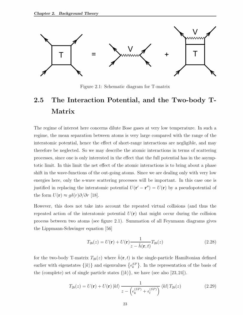
Chapter 2. Background Theory
TV
V
T= +
Figure 2.1: Schematic diagram for T-matrix
2.5 The Interaction Potential, and the Two-body T-
Matrix
The regime of interest here concerns dilute Bose gases at very low temperature. In such a
regime, the mean separation between atoms is very large compared with the range of the
interatomic potential, hence the effect of short-range interactions are negligible, and may
therefore be neglected. So we may describe the atomic interactions in terms of scattering
processes, since one is only interested in the effect that the full potential has in the asymp-
totic limit. In this limit the net effect of the atomic interactions is to bring about a phase
shift in the wave-functions of the out-going atoms. Since we are dealing only with very low
energies here, only the s-wave scattering processes will be important. In this case one is
justified in replacing the interatomic potential U(r′ − r′′) = U(r) by a pseudopotential of
the form U(r) ≈ gδ(r)∂/∂r [18].
However, this does not take into account the repeated virtual collisions (and thus the
repeated action of the interatomic potential U(r) that might occur during the collision
process between two atoms (see figure 2.1). Summation of all Feynmann diagrams gives
the Lippmann-Schwinger equation [56]
T2b(z) = U(r) + U(r)1
z − h(r, t)T2b(z) (2.28)
for the two-body T-matrix T2b(z) where h(r, t) is the single-particle Hamiltonian defined
earlier with eigenstates |k〉 and eigenvalues
ǫSPk
. In the representation of the basis of
the (complete) set of single particle states |k〉, we have (see also [23, 24]).
T2b(z) = U(r) + U(r) |kl〉 1
z −(
ǫ(SP )k + ǫ
(SP )l
) 〈kl| T2b(z) (2.29)
23
Chapter 2. Background Theory
and we would replace the bare atomic potential U(r) with the effective interaction potential
given by the two-body T-matrix T2b(z).
The contact potential approximation U(r) → gδ(r) would amount to replacing the two-
body T-matrix T2b(z) by the lowest-order approximation gδ(r). As we shall see later,
making the contact potential approximation leads to ultra-violet (UV) divergences in the
anomalous density (defined by equation (2.60)), which is important in mean-field theory
beyond the GPE approximation and in perturbation theories. Including higher order terms
for the T-matrix provides us with a suitable re-normalisation for the anomalous density,
and for energy shifts in perturbation theory. Alternatively, one can impose an energy
cut-off (thus eliminating higher energies) since the above treatment is valid only for low
energies. The problem here is that the results would depend on this cut-off. However, if
this cut-off is chosen judiciously, the errors in this analysis are expected to be relatively
small, hence this should not affect qualitatively the conclusions reached concerning the
precessional frequencies of vortices in harmonically trapped BECs, for example.
2.6 Mean Field Theories
We discuss two types of mean field theory here, namely symmetry-breaking mean-field
theories, and number-conserving mean-field theories.
2.6.1 Symmetry-breaking Mean field Theories
In symmetry-breaking theories, we replace the condensate operator Φ(r, t) in the expression
ψ(r, t) = Φ(r, t)+ η(r, t) with a c-field (i.e. we regard the condensate operator as a classical
field), thus
ψ(r, t) = Φ(r, t) + η(r, t) (2.30)
This is motivated by noting that the number of condensate atoms is given by Nc |Nc〉 =∫
drΦ†(r, t)Φ(r, t) |Nc〉 = Nc |Nc〉, and since
[
Φ(r, t), Φ†(r′, t)]
= δ(r− r′), (2.31)
we find that∫
drΦ(r, t)Φ†(r, t) |Nc〉 = (Nc +1) |Nc〉 ≈ Nc |Nc〉 for large Nc, so for Nc →∞,
we can regard Φ(r, t) and Φ†(r, t) as commuting, and hence we can regard Φ(r, t) as a
classical field Φ(r, t) in the thermodynamic limit. For a finite system, however, particle
24
Chapter 2. Background Theory
conservation violated. This can also be seen in the light of the breaking of U(1) symmetry.
The ansatz ψ(r, t) = Φ(r, t) + η(r, t) fixes the phase of the condensate. Since the total
number of particles and the global phase are canonically conjugate, this leads to a violation
of particle number conservation.
We can, however, fix the number of particles if we work in the Grand-Canonical Ensemble,
though this does lead to other issues, for example, the Grand-Canonical catastrophe [12,13]
(discussed later at the start of section 2.7). We thus obtain the following second-quantised
Grand-Canonical Hamiltonian [11]
H(GC)(t) =
∫
drψ†(r, t)(
h(r)− µ)
ψ(r, t)+1
2
∫ ∫
drdr′ψ†(r, t)ψ†(r′, t)U(r−r′)ψ(r′, t)ψ(r, t)
(2.32)
The Heisenberg equation of motion in the contact potential approximation is then given
by
i~∂
∂tψ(r, t) =
[
ψ(r, t), H(t)]
=(
h(r)− µ)
ψ(r, t) + gψ†(r, t)ψ(r, t)ψ(r, t) (2.33)
The inclusion of µ, the chemical potential, ensures that the total number of particles in the
system is fixed. Substituting the ansatz ψ(r, t) = Φ(r, t)+ η(r, t) into the Grand-Canonical
Bose Hamiltonian (2.32), we find in the contact potential approximation that
H(GC)(t) = H(GC)0 (t) + H
(GC)1 (t) + H
(GC)2 (t) + H
(GC)3 (t) + H
(GC)4 (t) (2.34)
where
H(GC)0 (t) =
∫
drΦ∗(
h− µ+ g2|Φ|2
)
Φ
H(GC)1 (t) =
∫
dr(
η†(
h− µ+ g |Φ|2)
Φ + Φ∗(
h− µ+ g |Φ|2)
η)
H(GC)2 (t) =
∫
dr(
η†(
h− µ+ 2g |Φ|2)
η + g2
(
Φ2η†η† + Φ∗2ηη))
H(GC)3 (t) = g
∫
dr(
Φη†η†η + Φ∗η†ηη)
H(GC)4 (t) = g
2
∫
drη†η†ηη.
(2.35)
The Gross-Pitaevskii Equation
To zeroth order in η, we can write [5–9]
i~∂
∂tΦ(r, t) =
δH0
δΦ∗ =(
h− µ+ g |Φ(r, t)|2)
Φ(r, t). (2.36)
This is the time-dependent Gross-Pitaevskii equation (GPE), and since we have neglected
the fluctuation operator completely, this equation is only valid at zero temperature (though
25
Chapter 2. Background Theory
it still neglects vacuum fluctuations at zero temperature). In spite of this, the GPE is
still very useful in many situations, and successfully yields the essential behaviour for
Bose-Einstein condensates (BECs) in many situations - for example, the precession of
vortices [36–40,79–83], the interference of two condensates [47], etc. The application of the
GPE has thus formed an industry in the field.
The Bogoliubov Approximation
One can apply linear response theory to the GPE [6–10] in order to determine the excitation
energies of the BEC at T ≈ 0. Writing
Φ(r, t) = e−i∆µt/~(
φ(r) + e−iǫt/~u(r) + eiǫt/~v∗(r))
(2.37)
where ∆µ is a shift in the chemical potential determined by the number of condensate
atoms given by the Bose-Einstein distribution (2.41), and retaining only terms to first
order in u(r) and v(r), and equating phase terms e−i∆µt/~, e−i(∆µ−ǫ)t/~ and e−i(∆µ+ǫ)t/~, we
obtain the time-independent GPE
∆µΦ(r) =(
h(r)− µ+ g |Φ(r)|2)
Φ(r) (2.38)
and the time-independent Bogoliubov de Gennes Equations (BdGEs)
ǫ
[
u(r)
v(r)
]
=
[
L0(r) M0(r)
−M∗0(r) −L∗
0(r)
][
u(r)
v(r)
]
(2.39)
L0(r) ≡ h(r)− µ+ 2g |Φ(r)|2
M0(r) ≡ gΦ2(r).(2.40)
Here the number of condensate atoms Nc is given by the Bose-Einstein distribution
Nc =1
exp(β∆µ)− 1(2.41)
and in the thermodynamic limit ∆µ→ 0. Here β ≡ 1/kBT is the temperature parameter,
with kB the Boltzmann constant and T the temperature in degrees Kelvin. In the regime of
interest (low temperatures, and macroscopic occupation of the ground state), ∆µ is negli-
gible, and can be ignored (see later), thus yielding the usual form for the time-independent
GPE
µΦ(r) =(
h(r) + g |Φ(r)|2)
Φ(r). (2.42)
The energy eigenvalues correspond to the collective excitation energies in the zero-temperature
limit (neglecting the thermal density), i.e. at T ≈ 0. This approximation is known as the
Bogoliubov approximation [10].
26
Chapter 2. Background Theory
We can also derive the BdGEs in the Bogoliubov approximation from the Heisenberg
equation of motion (2.27) by applying the Bogoliubov transformation
η(r, t) =∑
k
(
uk(r, t)ak + v∗k(r, t)a†k
)
(2.43)
for the fluctuation operator η(r, t), with Hermitian conjugate
η†(r, t) =∑
k
(
vk(r, t)ak + u∗k(r, t)a†k
)
. (2.44)
Here we have expanded the fluctuation operator η(r, t) in a weakly-interacting quasi-
particle basis. The assumption here is that the quasi-particles are non-interacting. The
operators a†k and ak are creation and annihilation operators for these quasi-particles, and
the uk(r, t) and v∗k(r, t) are the associated quasi-particle amplitudes. This transformation
is canonical, hence the Bose commutation relations are preserved, i.e.
[
ak, a†l
]
= δk,l and [ak, al] =[
a†k, a†l
]
= 0. (2.45)
The creation and annihilation operators a†k and ak are given in terms of the fluctuation
operator η(r, t), and the quasi-particle amplitudes uk(r, t) and v∗k(r, t) by the inverse Bo-
goliubov transformation
ak =
∫
dr(
u∗k(r, t)η(r, t)− v∗k(r, t)η†(r, t))
(2.46)
with Hermitian conjugate
a†k =
∫
dr(
−vk(r, t)η(r, t) + uk(r, t)η†(r, t)
)
. (2.47)
Then, using the commutation relations
[
ψ(r, t), a†q
]
= uq(r, t),[
aq, ψ(r, t)]
= v∗q (r, t),[
ψ†(r, t), a†q
]
= vq(r, t),[
aq, ψ†(r, t)
]
= u∗q(r, t),
(2.48)
we find to first order in η(r, t)
i~∂uq(r, t)
∂t=(
h(r)− µ+ 2g |Φ(r, t)|2)
uq(r, t) + gΦ2(r, t)vq(r, t)
and
i~∂v∗q (r, t)
∂t=(
h(r)− µ+ 2g |Φ(r, t)|2)
v∗q (r, t) + gΦ2(r, t)u∗q(r, t)
which yields the BdGEs
i~ ∂∂t
[
uq(r, t)
vq(r, t)
]
=
[
L0(r, t) M0(r, t)
−M∗0(r, t) −L∗
0(r, t)
][
uq(r, t)
vq(r, t)
]
(2.49)
27
Chapter 2. Background Theory
in the Bogoliubov approximation.
The corresponding time-independent BdGEs are
ǫq
[
uq(r)
vq(r)
]
=
[
L0(r) M0(r)
−M∗0(r) −L∗
0(r)
][
uq(r)
vq(r)
]
. (2.50)
The quasi-particle occupation numbers are given by the Bose distribution
NBE(ǫq) =1
exp(βǫq)− 1, (2.51)
hence one can calculate the mean thermal density
n(r, t) ≡⟨
η†(r, t)η(r, t)⟩
=∑
q
[
|uq(r, t)|2NBE(ǫq) + |vq(r, t)|2 (NBE(ǫq) + 1)]
. (2.52)
Since the Bogoliubov transformation is canonical, and hence the commutation relations
(2.45) hold, the following orthogonality and symmetry relations for the quasi-particle am-
plitudes∫
dr (u∗k(r, t)ul(r, t)− v∗k(r, t)vl(r, t)) = δk,l∫
dr (u∗k(r, t)v∗l (r, t)− v∗k(r, t)u∗l (r, t)) = 0
∫
dr (uk(r, t)vl(r, t)− vk(r, t)ul(r, t)) = 0
(2.53)
must also hold, thus establishing the normalisation condition∫
dr(
|uk(r, t)|2 − |vk(r, t)|2)
= 1 (2.54)
for the quasi-particle amplitudes.
The linear response treatment demonstrates, in the presence of a condensate, the equiva-
lence of the collective modes and the quasi-particle excitations. We therefore associate the
Bogoliubov energy spectrum with the collective excitations at T = 0.
The Hartree-Fock-Bogoliubov (HFB) Equations
We can use the factorisation approximations [11]
η†(r, t)η(r, t)η(r, t) ≈ 2n(r, t)η(r, t) + m(r, t)η†(r, t)
η†(r, t)η†(r, t)η(r, t) ≈ 2n(r, t)η†(r, t) + m∗(r, t)η(r, t)
η†(r, t)η†(r, t)η(r, t)η(r, t) ≈ 4n(r, t)η†(r, t)η(r, t) + m(r, t)η†(r, t)η†(r, t)
+m∗(r, t)η(r, t)η(r, t)− 2n2(r, t)− |m(r, t)|2
(2.55)
to obtain the quadratic approximation in η and η† for the Grand-Canonical Hamiltonian
H(GC)(t) ≈ HHFB(t) (2.56)
28
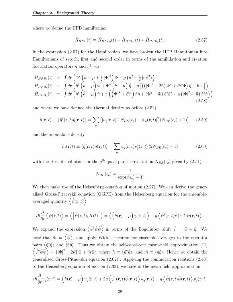
Chapter 2. Background Theory
where we define the HFB hamiltonian
HHFB(t) ≡ HHFB0(t) + HHFB1(t) + HHFB2(t). (2.57)
In the expression (2.57) for the Hamiltonian, we have broken the HFB Hamiltonian into
Hamiltonians of zeroth, first and second order in terms of the annihilation and creation
fluctuation operators η and η†, viz.
HHFB0(t) ≡∫
dr(
Φ∗(
h− µ+ g2|Φ|2
)
Φ− g(
n2 + 12|m|2
)
)
HHFB1(t) ≡∫
dr(
η†(
h− µ)
Φ + Φ∗(
h− µ)
η + g[((
|Φ|2 + 2n)
Φ∗ + m∗Φ)
η + h.c.]
)
HHFB2(t) ≡∫
dr(
η†(
h− µ)
η + g2
((
Φ∗2+ m∗
)
ηη + (Φ2 + m) η†η† + 4(
|Φ|2 + n)
η†η))
(2.58)
and where we have defined the thermal density as before (2.52)
n(r, t) ≡⟨
η†(r, t)η(r, t)⟩
=∑
q
[
|uq(r, t)|2NBE(ǫq) + |vq(r, t)|2 (NBE(ǫq) + 1)]
(2.59)
and the anomalous density
m(r, t) ≡ 〈η(r, t)η(r, t)〉 =∑
q
uq(r, t)v∗q(r, t) (2NBE(ǫq) + 1) (2.60)
with the Bose distribution for the qth quasi-particle excitation NBE(ǫq) given by (2.51)
NBE(ǫq) =1
exp(βǫq)− 1.
We then make use of the Heisenberg equation of motion (2.27). We can derive the gener-
alised Gross-Pitaevskii equation (GGPE) from the Heisenberg equation for the ensemble-
averaged quantity⟨
ψ(r, t)⟩
i~∂
∂t
⟨
ψ(r, t)⟩
=⟨[
ψ(r, t), H(t)]⟩
=⟨(
h(r)− µ)
ψ(r, t)⟩
+ g⟨
ψ†(r, t)ψ(r, t)ψ(r, t)⟩
.
We expand the expression⟨
ψ†ψψ⟩
in terms of the Bogoliubov shift ψ = Φ + η. We
note that Φ =⟨
ψ⟩
, and apply Wick’s theorem for ensemble averages to the operator
pairs⟨
η†η⟩
and 〈ηη〉. Thus we obtain the self-consistent mean-field approximation [11]⟨
ψ†ψψ⟩
=(
|Φ|2 + 2n)
Φ + mΦ∗, where n ≡⟨
η†η⟩
, and m ≡ 〈ηη〉. Hence we obtain the
generalised Gross-Pitaevskii equation (2.62) . Applying the commutation relations (2.48)
to the Heisenberg equation of motion (2.33), we have in the mean field approximation
i~∂
∂tuq(r, t) =
(
h(r)− µ)
uq(r, t) + 2g⟨
ψ†(r, t)ψ(r, t)⟩
uq(r, t) + g⟨
ψ(r, t)ψ(r, t)⟩
vq(r, t)
29
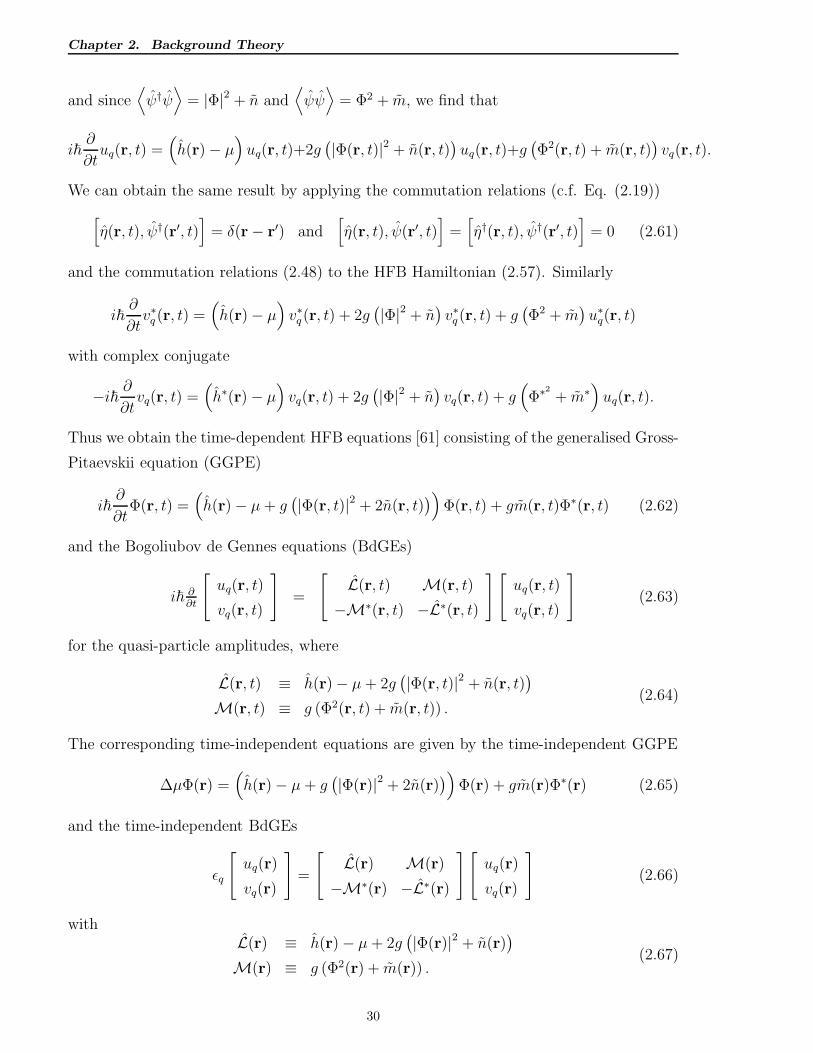
Chapter 2. Background Theory
and since⟨
ψ†ψ⟩
= |Φ|2 + n and⟨
ψψ⟩
= Φ2 + m, we find that
i~∂
∂tuq(r, t) =
(
h(r)− µ)
uq(r, t)+2g(
|Φ(r, t)|2 + n(r, t))
uq(r, t)+g(
Φ2(r, t) + m(r, t))
vq(r, t).
We can obtain the same result by applying the commutation relations (c.f. Eq. (2.19))
[
η(r, t), ψ†(r′, t)]
= δ(r− r′) and[
η(r, t), ψ(r′, t)]
=[
η†(r, t), ψ†(r′, t)]
= 0 (2.61)
and the commutation relations (2.48) to the HFB Hamiltonian (2.57). Similarly
i~∂
∂tv∗q (r, t) =
(
h(r)− µ)
v∗q (r, t) + 2g(
|Φ|2 + n)
v∗q (r, t) + g(
Φ2 + m)
u∗q(r, t)
with complex conjugate
−i~ ∂∂tvq(r, t) =
(
h∗(r)− µ)
vq(r, t) + 2g(
|Φ|2 + n)
vq(r, t) + g(
Φ∗2
+ m∗)
uq(r, t).
Thus we obtain the time-dependent HFB equations [61] consisting of the generalised Gross-
Pitaevskii equation (GGPE)
i~∂
∂tΦ(r, t) =
(
h(r)− µ+ g(
|Φ(r, t)|2 + 2n(r, t))
)
Φ(r, t) + gm(r, t)Φ∗(r, t) (2.62)
and the Bogoliubov de Gennes equations (BdGEs)
i~ ∂∂t
[
uq(r, t)
vq(r, t)
]
=
[
L(r, t) M(r, t)
−M∗(r, t) −L∗(r, t)
][
uq(r, t)
vq(r, t)
]
(2.63)
for the quasi-particle amplitudes, where
L(r, t) ≡ h(r)− µ+ 2g(
|Φ(r, t)|2 + n(r, t))
M(r, t) ≡ g (Φ2(r, t) + m(r, t)) .(2.64)
The corresponding time-independent equations are given by the time-independent GGPE
∆µΦ(r) =(
h(r)− µ+ g(
|Φ(r)|2 + 2n(r))
)
Φ(r) + gm(r)Φ∗(r) (2.65)
and the time-independent BdGEs
ǫq
[
uq(r)
vq(r)
]
=
[
L(r) M(r)
−M∗(r) −L∗(r)
][
uq(r)
vq(r)
]
(2.66)
withL(r) ≡ h(r)− µ+ 2g
(
|Φ(r)|2 + n(r))
M(r) ≡ g (Φ2(r) + m(r)) .(2.67)
30
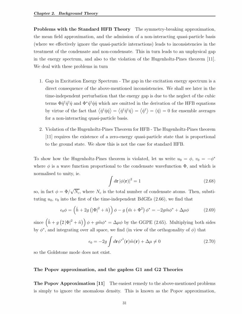
Chapter 2. Background Theory
Problems with the Standard HFB Theory The symmetry-breaking approximation,
the mean field approximation, and the admission of a non-interacting quasi-particle basis
(where we effectively ignore the quasi-particle interactions) leads to inconsistencies in the
treatment of the condensate and non-condensate. This in turn leads to an unphysical gap
in the energy spectrum, and also to the violation of the Hugenholtz-Pines theorem [11].
We deal with these problems in turn
1. Gap in Excitation Energy Spectrum - The gap in the excitation energy spectrum is a
direct consequence of the above-mentioned inconsistencies. We shall see later in the
time-independent perturbation that the energy gap is due to the neglect of the cubic
terms Φη†η†η and Φ∗η†ηη which are omitted in the derivation of the HFB equations
by virtue of the fact that⟨
η†ηη⟩
=⟨
η†η†η⟩
=⟨
η†⟩
= 〈η〉 = 0 for ensemble averages
for a non-interacting quasi-particle basis.
2. Violation of the Hugenholtz-Pines Theorem for HFB - The Hugenholtz-Pines theorem
[11] requires the existence of a zero-energy quasi-particle state that is proportional
to the ground state. We show this is not the case for standard HFB.
To show how the Hugenholtz-Pines theorem is violated, let us write u0 = φ, v0 = −φ∗
where φ is a wave function proportional to the condensate wavefunction Φ, and which is
normalised to unity, ie.∫
dr |φ(r)|2 = 1 (2.68)
so, in fact φ = Φ/√Nc, where Nc is the total number of condensate atoms. Then, substi-
tuting u0, v0 into the first of the time-independent BdGEs (2.66), we find that
ǫ0φ =(
h+ 2g(
|Φ|2 + n)
)
φ− g(
m+ Φ2)
φ∗ = −2gmφ∗ + ∆µφ (2.69)
since(
h + g(
2 |Φ|2 + n)
)
φ + gmφ∗ = ∆µφ by the GGPE (2.65). Multiplying both sides
by φ∗, and integrating over all space, we find (in view of the orthogonality of φ) that
ǫ0 = −2g
∫
drφ∗2
(r)m(r) + ∆µ 6= 0 (2.70)
so the Goldstone mode does not exist.
The Popov approximation, and the gapless G1 and G2 Theories
The Popov Approximation [11] The easiest remedy to the above-mentioned problems
is simply to ignore the anomalous density. This is known as the Popov approximation,
31
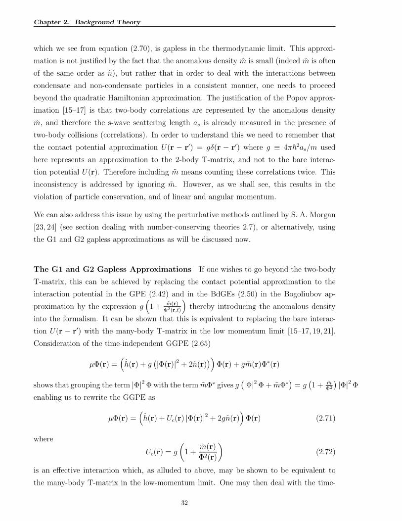
Chapter 2. Background Theory
which we see from equation (2.70), is gapless in the thermodynamic limit. This approxi-
mation is not justified by the fact that the anomalous density m is small (indeed m is often
of the same order as n), but rather that in order to deal with the interactions between
condensate and non-condensate particles in a consistent manner, one needs to proceed
beyond the quadratic Hamiltonian approximation. The justification of the Popov approx-
imation [15–17] is that two-body correlations are represented by the anomalous density
m, and therefore the s-wave scattering length as is already measured in the presence of
two-body collisions (correlations). In order to understand this we need to remember that
the contact potential approximation U(r − r′) = gδ(r − r′) where g ≡ 4π~2as/m used
here represents an approximation to the 2-body T-matrix, and not to the bare interac-
tion potential U(r). Therefore including m means counting these correlations twice. This
inconsistency is addressed by ignoring m. However, as we shall see, this results in the
violation of particle conservation, and of linear and angular momentum.
We can also address this issue by using the perturbative methods outlined by S. A. Morgan
[23, 24] (see section dealing with number-conserving theories 2.7), or alternatively, using
the G1 and G2 gapless approximations as will be discussed now.
The G1 and G2 Gapless Approximations If one wishes to go beyond the two-body
T-matrix, this can be achieved by replacing the contact potential approximation to the
interaction potential in the GPE (2.42) and in the BdGEs (2.50) in the Bogoliubov ap-
proximation by the expression g(
1 + m(r)Φ2(r,t)
)
thereby introducing the anomalous density
into the formalism. It can be shown that this is equivalent to replacing the bare interac-
tion U(r − r′) with the many-body T-matrix in the low momentum limit [15–17, 19, 21].
Consideration of the time-independent GGPE (2.65)
µΦ(r) =(
h(r) + g(
|Φ(r)|2 + 2n(r))
)
Φ(r) + gm(r)Φ∗(r)
shows that grouping the term |Φ|2 Φ with the term mΦ∗ gives g(
|Φ|2 Φ + mΦ∗) = g(
1 + mΦ2
)
|Φ|2 Φ
enabling us to rewrite the GGPE as
µΦ(r) =(
h(r) + Uc(r) |Φ(r)|2 + 2gn(r))
Φ(r) (2.71)
where
Uc(r) = g
(
1 +m(r)
Φ2(r)
)
(2.72)
is an effective interaction which, as alluded to above, may be shown to be equivalent to
the many-body T-matrix in the low-momentum limit. One may then deal with the time-
32
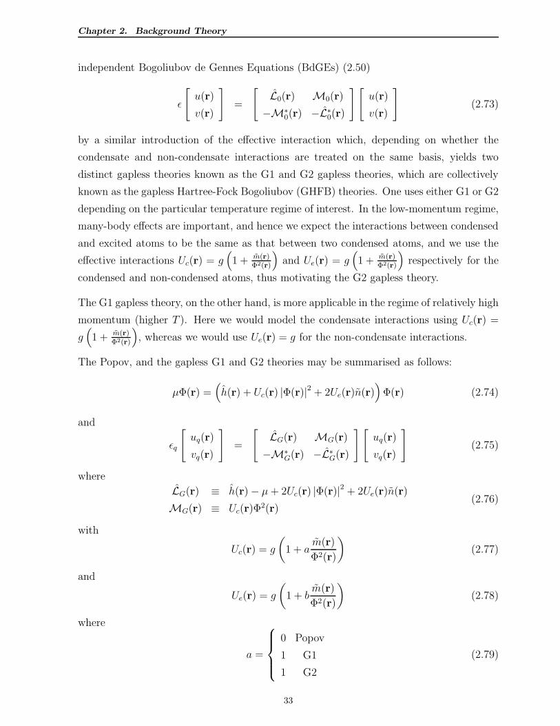
Chapter 2. Background Theory
independent Bogoliubov de Gennes Equations (BdGEs) (2.50)
ǫ
[
u(r)
v(r)
]
=
[
L0(r) M0(r)
−M∗0(r) −L∗
0(r)
][
u(r)
v(r)
]
(2.73)
by a similar introduction of the effective interaction which, depending on whether the
condensate and non-condensate interactions are treated on the same basis, yields two
distinct gapless theories known as the G1 and G2 gapless theories, which are collectively
known as the gapless Hartree-Fock Bogoliubov (GHFB) theories. One uses either G1 or G2
depending on the particular temperature regime of interest. In the low-momentum regime,
many-body effects are important, and hence we expect the interactions between condensed
and excited atoms to be the same as that between two condensed atoms, and we use the
effective interactions Uc(r) = g(
1 + m(r)Φ2(r)
)
and Ue(r) = g(
1 + m(r)Φ2(r)
)
respectively for the
condensed and non-condensed atoms, thus motivating the G2 gapless theory.
The G1 gapless theory, on the other hand, is more applicable in the regime of relatively high
momentum (higher T ). Here we would model the condensate interactions using Uc(r) =
g(
1 + m(r)Φ2(r)
)
, whereas we would use Ue(r) = g for the non-condensate interactions.
The Popov, and the gapless G1 and G2 theories may be summarised as follows:
µΦ(r) =(
h(r) + Uc(r) |Φ(r)|2 + 2Ue(r)n(r))
Φ(r) (2.74)
and
ǫq
[
uq(r)
vq(r)
]
=
[
LG(r) MG(r)
−M∗G(r) −L∗
G(r)
][
uq(r)
vq(r)
]
(2.75)
where
LG(r) ≡ h(r)− µ+ 2Uc(r) |Φ(r)|2 + 2Ue(r)n(r)
MG(r) ≡ Uc(r)Φ2(r)
(2.76)
with
Uc(r) = g
(
1 + am(r)
Φ2(r)
)
(2.77)
and
Ue(r) = g
(
1 + bm(r)
Φ2(r)
)
(2.78)
where
a =
0 Popov
1 G1
1 G2
(2.79)
33
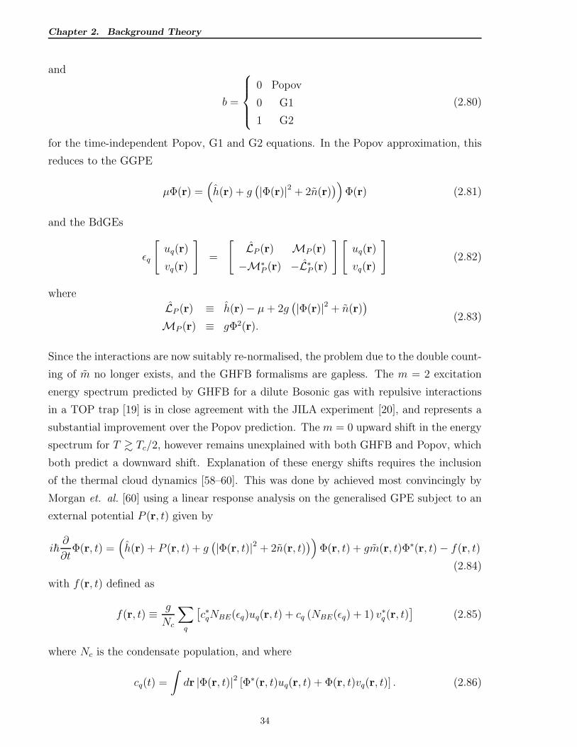
Chapter 2. Background Theory
and
b =
0 Popov
0 G1
1 G2
(2.80)
for the time-independent Popov, G1 and G2 equations. In the Popov approximation, this
reduces to the GGPE
µΦ(r) =(
h(r) + g(
|Φ(r)|2 + 2n(r))
)
Φ(r) (2.81)
and the BdGEs
ǫq
[
uq(r)
vq(r)
]
=
[
LP (r) MP (r)
−M∗P (r) −L∗
P (r)
][
uq(r)
vq(r)
]
(2.82)
where
LP (r) ≡ h(r)− µ+ 2g(
|Φ(r)|2 + n(r))
MP (r) ≡ gΦ2(r).(2.83)
Since the interactions are now suitably re-normalised, the problem due to the double count-
ing of m no longer exists, and the GHFB formalisms are gapless. The m = 2 excitation
energy spectrum predicted by GHFB for a dilute Bosonic gas with repulsive interactions
in a TOP trap [19] is in close agreement with the JILA experiment [20], and represents a
substantial improvement over the Popov prediction. The m = 0 upward shift in the energy
spectrum for T & Tc/2, however remains unexplained with both GHFB and Popov, which
both predict a downward shift. Explanation of these energy shifts requires the inclusion
of the thermal cloud dynamics [58–60]. This was done by achieved most convincingly by
Morgan et. al. [60] using a linear response analysis on the generalised GPE subject to an
external potential P (r, t) given by
i~∂
∂tΦ(r, t) =
(
h(r) + P (r, t) + g(
|Φ(r, t)|2 + 2n(r, t))
)
Φ(r, t) + gm(r, t)Φ∗(r, t)− f(r, t)
(2.84)
with f(r, t) defined as
f(r, t) ≡ g
Nc
∑
q
[
c∗qNBE(ǫq)uq(r, t) + cq (NBE(ǫq) + 1) v∗q (r, t)]
(2.85)
where Nc is the condensate population, and where
cq(t) =
∫
dr |Φ(r, t)|2 [Φ∗(r, t)uq(r, t) + Φ(r, t)vq(r, t)] . (2.86)
34
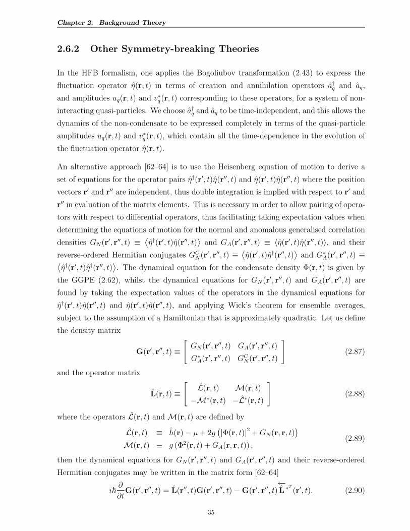
Chapter 2. Background Theory
2.6.2 Other Symmetry-breaking Theories
In the HFB formalism, one applies the Bogoliubov transformation (2.43) to express the
fluctuation operator η(r, t) in terms of creation and annihilation operators a†q and aq,
and amplitudes uq(r, t) and v∗q (r, t) corresponding to these operators, for a system of non-
interacting quasi-particles. We choose a†q and aq to be time-independent, and this allows the
dynamics of the non-condensate to be expressed completely in terms of the quasi-particle
amplitudes uq(r, t) and v∗q (r, t), which contain all the time-dependence in the evolution of
the fluctuation operator η(r, t).
An alternative approach [62–64] is to use the Heisenberg equation of motion to derive a
set of equations for the operator pairs η†(r′, t)η(r′′, t) and η(r′, t)η(r′′, t) where the position
vectors r′ and r′′ are independent, thus double integration is implied with respect to r′ and
r′′ in evaluation of the matrix elements. This is necessary in order to allow pairing of opera-
tors with respect to differential operators, thus facilitating taking expectation values when
determining the equations of motion for the normal and anomalous generalised correlation
densities GN(r′, r′′, t) ≡⟨
η†(r′, t)η(r′′, t)⟩
and GA(r′, r′′, t) ≡ 〈η(r′, t)η(r′′, t)〉, and their
reverse-ordered Hermitian conjugates GCN(r′, r′′, t) ≡
⟨
η(r′, t)η†(r′′, t)⟩
and G∗A(r′, r′′, t) ≡
⟨
η†(r′, t)η†(r′′, t)⟩
. The dynamical equation for the condensate density Φ(r, t) is given by
the GGPE (2.62), whilst the dynamical equations for GN(r′, r′′, t) and GA(r′, r′′, t) are
found by taking the expectation values of the operators in the dynamical equations for
η†(r′, t)η(r′′, t) and η(r′, t)η(r′′, t), and applying Wick’s theorem for ensemble averages,
subject to the assumption of a Hamiltonian that is approximately quadratic. Let us define
the density matrix
G(r′, r′′, t) ≡[
GN(r′, r′′, t) GA(r′, r′′, t)
G∗A(r′, r′′, t) GC
N(r′, r′′, t)
]
(2.87)
and the operator matrix
L(r, t) ≡[
L(r, t) M(r, t)
−M∗(r, t) −L∗(r, t)
]
(2.88)
where the operators L(r, t) andM(r, t) are defined by
L(r, t) ≡ h(r)− µ+ 2g(
|Φ(r, t)|2 +GN(r, r, t))
M(r, t) ≡ g (Φ2(r, t) +GA(r, r, t)) ,(2.89)
then the dynamical equations for GN(r′, r′′, t) and GA(r′, r′′, t) and their reverse-ordered
Hermitian conjugates may be written in the matrix form [62–64]
i~∂
∂tG(r′, r′′, t) = L(r′′, t)G(r′, r′′, t)−G(r′, r′′, t)
←−L ∗T
(r′, t). (2.90)
35
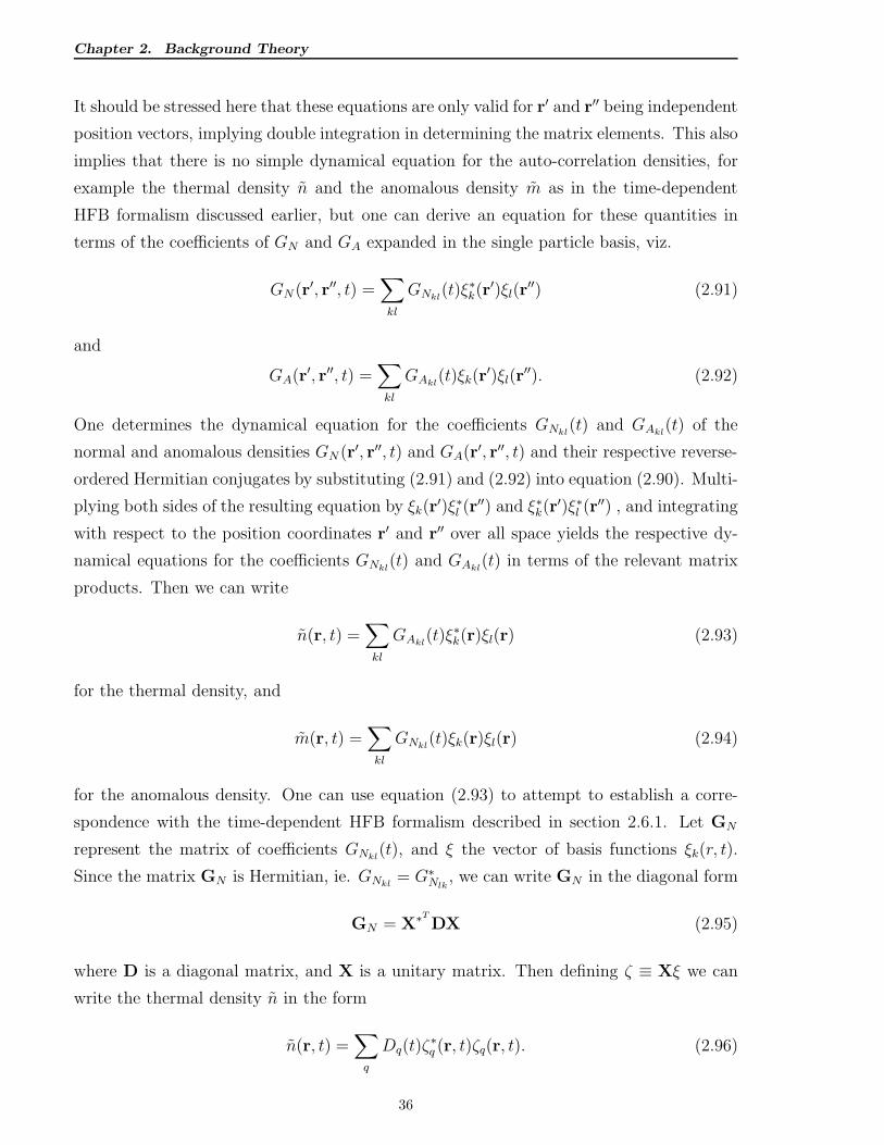
Chapter 2. Background Theory
It should be stressed here that these equations are only valid for r′ and r′′ being independent
position vectors, implying double integration in determining the matrix elements. This also
implies that there is no simple dynamical equation for the auto-correlation densities, for
example the thermal density n and the anomalous density m as in the time-dependent
HFB formalism discussed earlier, but one can derive an equation for these quantities in
terms of the coefficients of GN and GA expanded in the single particle basis, viz.
GN (r′, r′′, t) =∑
kl
GNkl(t)ξ∗k(r
′)ξl(r′′) (2.91)
and
GA(r′, r′′, t) =∑
kl
GAkl(t)ξk(r
′)ξl(r′′). (2.92)
One determines the dynamical equation for the coefficients GNkl(t) and GAkl
(t) of the
normal and anomalous densities GN (r′, r′′, t) and GA(r′, r′′, t) and their respective reverse-
ordered Hermitian conjugates by substituting (2.91) and (2.92) into equation (2.90). Multi-
plying both sides of the resulting equation by ξk(r′)ξ∗l (r
′′) and ξ∗k(r′)ξ∗l (r
′′) , and integrating
with respect to the position coordinates r′ and r′′ over all space yields the respective dy-
namical equations for the coefficients GNkl(t) and GAkl
(t) in terms of the relevant matrix
products. Then we can write
n(r, t) =∑
kl
GAkl(t)ξ∗k(r)ξl(r) (2.93)
for the thermal density, and
m(r, t) =∑
kl
GNkl(t)ξk(r)ξl(r) (2.94)
for the anomalous density. One can use equation (2.93) to attempt to establish a corre-
spondence with the time-dependent HFB formalism described in section 2.6.1. Let GN
represent the matrix of coefficients GNkl(t), and ξ the vector of basis functions ξk(r, t).
Since the matrix GN is Hermitian, ie. GNkl= G∗
Nlk, we can write GN in the diagonal form
GN = X∗T
DX (2.95)
where D is a diagonal matrix, and X is a unitary matrix. Then defining ζ ≡ Xξ we can
write the thermal density n in the form
n(r, t) =∑
q
Dq(t)ζ∗q (r, t)ζq(r, t). (2.96)
36
Chapter 2. Background Theory
It is interesting to compare this with the thermal density n in the HFB formalism given
by (2.52). Since X is unitary,∫
drζ∗T
(r, t)ζ(r, t) =
∫
drX∗T
ξ∗T
(r, t)ξ(r, t)X = X∗T
X = I, (2.97)
i.e.∫
drζ∗q (r, t)ζq(r, t) = 1, in contrast to the normalisation condition (2.54) for the quasi-
particle amplitudes uq and vq in HFB. One might be tempted to associate uq ≡ ςq and
vq ≡ 0, but this implies m ≡ 0 and is inconsistent with (2.94) where m is certainly not
zero. We conclude therefore that, whilst similar, this theory is not equivalent to the HFB
formalism discussed in section 2.6.1. In HFB we assume the existence of a non-interacting
quasi-particle basis, whereas no such assumption has been made here.
2.7 Number-conserving Theories
As already mentioned, the symmetry-breaking approach breaks the U(1) symmetry, and
hence overall number conservation is violated. One overcomes this problem by working in
the Grand-Canonical ensemble where the self-consistent calculation of the chemical poten-
tial µ and suitable normalisation of the quasi-particle amplitudes and of the condensate
fixes the overall problem. However this has implications for the fluctuations with variance
δ2n0
=(
1−(
TTc
)η)2
N2, where η is a trap-dependent exponent, and implies the unusual
scaling of δ2n0∝ N2 [12, 13] leading to the Grand-Canonical catastrophe. This arises from
the inconsistency of the symmetry-breaking treatment for a finite number of particles.
In number-conserving approaches, one maintains the U(1) symmetry (and hence maintains
particle conservation) by avoiding the broken symmetry ansatz. One also aims to achieve
a systematic expansion of the Hamiltonian which facilitates a perturbative approach. To
lowest order, the symmetry-breaking and number-conserving approaches lead to essentially
the same equations, namely the GPE (2.42) and the BdGEs (2.50) in the Bogoliubov
approximation. There are various ways by which this might be achieved:
2.7.1 The approach due to C. W. Gardiner
Homogeneous Bose gas In his paper [22], C. W. Gardiner considers the Hamiltonian
(in momentum space)
H =∑
k
~ωkb†kbk +
g
2
∑
k1,k2,k3,k4
b†k1b†k2bk3 bk4δk1+k2,k3+k4 . (2.98)
37
Chapter 2. Background Theory
He defines an annihilation operator A for the total number of particles, thus N = A†A
is the overall number operator. He defines phonon creation and annihilation operators β†k
and βk for the excitations in mode k in terms of the single-particle operators ak in by
βk ≡1√
Nb†0bk (2.99)
and shows that
b0 = A
(
1−∑
k 6=0 nk
2N
)
≈ A
in the limit N → ∞. The operators βk obey the Bose commutator relations (approxi-
mately) to order 1/N , i.e.
[
βk, β†k′
]
= δk,k′ − 1
Nbkb
†k′ ≈ δk,k′. (2.100)
Inhomogeneous Bose gas In the spatially inhomogeneous case, the Hamiltonian may
be written as
H =
∫
dr
(
ψ†(r, t)h(r)ψ(r, t) +g
2
∫
drψ†(r, t)ψ†(r, t)ψ(r, t)ψ(r, t)
)
(2.101)
He reformulates the system Hamiltonian (2.101), and the Bose field operator ψ(r, t), which
is expanded in terms the annihilation operator A, a condensate wave-function φ, and a
phonon field operator Λ (see below), performing an asymptotic expansion of the Hamilto-
nian in powers of√
N ,
H ≈ NH0 +√
NH1 + H2 (2.102)
where
H0 =∫
dr(
φ∗hφ+ 12gN |φ|4
)
H1 =∫
dr(
Λ†hφ+ Λhφ∗ + gN |φ|2(
φΛ† + φ∗Λ))
H2 =∫
dr(
Λ†hΛ + 12gN(
φ2Λ†Λ† + φ∗2ΛΛ)
+ Λ†Λ(
2gN |φ|2 − µ)
− 12gN |φ|4
)
(2.103)
and where
µ =
∫
dr(
φ∗(r, t)h(r)φ(r, t) + gN |φ(r, t)|4)
(2.104)
The field particle operator is approximated by
ψ(r, t) ≈ A
(
φ(r, t) +1√N
Λ(r, t)
)
(2.105)
38
Chapter 2. Background Theory
where φ(r) is the condensate wave-function normalised to unity, and Λ(r) is a phonon field
operator defined by
Λ(r, t) ≡∑
k
φk(r)bk. (2.106)
Choosing φ to minimize H subject to the normalization condition∫
dr |φ(r, t)|2 = 1, he
obtains the time-independent Gross-Pitaevskii equation(
h + gN |φ(r)|2)
φ(r) = µφ(r) (2.107)
Making the Bogoliubov transformation
bk =∑
m
(
ckmam + dkma†m
)
(2.108)
we can write
Λ(r, t) =∑
m
(
um(r, t)am + v∗m(r, t)a†m)
(2.109)
where
um(r, t) ≡∑k ckmφ(r) and um(r, t) ≡∑k ckmφ(r) (2.110)
in terms of quasi-particles with creation and annihilation operators a†k and ak, we can then
write the Hamiltonian H2 in diagonal form
H2 = ~ωg(N) +∑
m
~ǫm(N)a†kak (2.111)
where ǫm(N) are the excitation energies of the quasi-particles.
Applicability In view of the approximations implied by the number-conserving ansatz
(2.105), and the omission of the thermal density (this is essentially the GPE), this theory
is only valid at T = 0.
2.7.2 The approach due to S. A. Morgan
A number-conserving, finite-temperature analysis incorporating second-order perturbation
theory was performed by S. A. Morgan [23, 24]. In his analysis, he defines the number
conserving operators by αk = a†0bk where a0 =(
N0 + 1)1/2
b0 with N0 = b†0b0 the operator
for the condensate number, and bk are the mode operators for the basis functions φi(r)in the Bose Hamiltonian
ˆH(t) =∞∑
k,l=1
〈k| h |l〉 b†k bl +1
2
∞∑
k,l,m,n=1
〈kl|U (S) |mn〉 b†k b†l bnbm (2.112)
39
Chapter 2. Background Theory
where 〈k| h |l〉 =∫
drφ∗k(r)h(r)φl(r), and U (S) is the symmetrised interaction potential
defined by 〈kl|U (S) |mn〉 = 12[〈kl|U |mn〉 + 〈lk|U |mn〉] with
〈kl|U |mn〉 =
∫
dr
∫
dr′φ∗k(r)φ
∗l (r
′)U(r − r′)φm(r′)φn(r)
where U(r − r′) is the effective atomic potential. He rewrites the Hamiltonian as follows
[23, 24]
H = H0 + H1 + H2 + H3 + H4 (2.113)
where
H0 =√
N0
(
〈0| h |0〉+ 1
2N0 〈00|U (S) |00〉
)
(2.114)
H1 =√
N0
∑
k 6=0
(
〈k| h |0〉+ 1
2〈k0|U (S) |00〉
)
b†k + h.c. (2.115)
H2 =∑
k,l 6=0
(
〈k| h |l〉 − λδk,l + 2N0 〈0k|U (S) |l0〉)
b†k bl+∑
k,l 6=0
(
N0
2〈kl|U (S) |00〉 b†k b
†l + h.c.
)
+λ⟨
Nex
⟩
(2.116)
H3 =∑
k,l,m6=0
(
√
N0 〈kl|U (S) |m0〉 b†k b†l bm + h.c.
)
(2.117)
H4 =∑
k,l,m6=0
1
2〈kl|U (S) |mn〉 b†k b
†l bmbn (2.118)
and
Nex =∑
k 6=0
b†k bk (2.119)
is the number operator for the non-condensate.⟨
Nex
⟩
is the ensemble-averaged quantum
expectation value, and is the mean occupation for the non-condensate. N0 is the mean
condensate population, and is defined by N0 = N −⟨
Nex
⟩
.
He first considers the terms in H to quadratic order, ie. H0, H1, and H2. The parameter
λ is defined by λ ≡ 〈0| h |0〉 +N0 〈00|U (S) |00〉 and is merely the condensate eigenstate as
calculated for the GPE. Minimization of H0 yields the GPE
〈k| h |0〉+N0 〈k0|U (S) |00〉 = λδk,0
which in the position representation using the contact potential approximation U(r) =
gδ(r) with g = 4π~2as/m, r = r1 − r2 where as is the s-wave scattering length, and m is
the atomic mass is given by
(
h+ gN |φ0(r)|2)
φ0(r) = λφ0(r). (2.120)
40
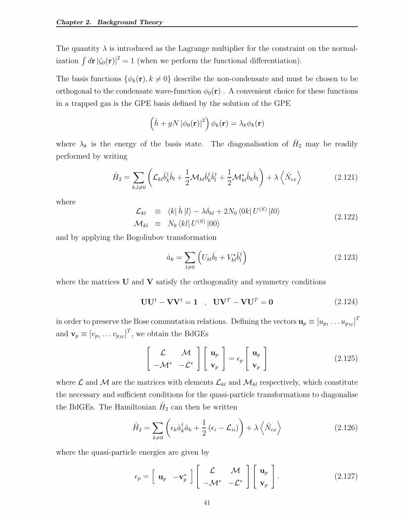
Chapter 2. Background Theory
The quantity λ is introduced as the Lagrange multiplier for the constraint on the normal-
ization∫
dr |ζ0(r)|2 = 1 (when we perform the functional differentiation).
The basis functions φk(r), k 6= 0 describe the non-condensate and must be chosen to be
orthogonal to the condensate wave-function φ0(r) . A convenient choice for these functions
in a trapped gas is the GPE basis defined by the solution of the GPE
(
h+ gN |φ0(r)|2)
φk(r) = λkφk(r)
where λk is the energy of the basis state. The diagonalisation of H2 may be readily
performed by writing
H2 =∑
k,l 6=0
(
Lklb†k bl +
1
2Mklb
†k b
†l +
1
2M∗
klbk bl
)
+ λ⟨
Nex
⟩
(2.121)
whereLkl ≡ 〈k| h |l〉 − λδkl + 2N0 〈0k|U (S) |l0〉Mkl ≡ N0 〈kl|U (S) |00〉
(2.122)
and by applying the Bogoliubov transformation
ak =∑
l 6=0
(
Uklbl + V ∗klb
†l
)
(2.123)
where the matrices U and V satisfy the orthogonality and symmetry conditions
UU† −VV† = 1 , UVT −VUT = 0 (2.124)
in order to preserve the Bose commutation relations. Defining the vectors up ≡ [up1 . . . upM]T
and vp ≡ [vp1 . . . vpM]T , we obtain the BdGEs
[
L M−M∗ −L∗
][
up
vp
]
= ǫp
[
up
vp
]
(2.125)
where L andM are the matrices with elements Lkl andMkl respectively, which constitute
the necessary and sufficient conditions for the quasi-particle transformations to diagonalise
the BdGEs. The Hamiltonian H2 can then be written
H2 =∑
k 6=0
(
ǫka†kak +
1
2(ǫi − Lii)
)
+ λ⟨
Nex
⟩
(2.126)
where the quasi-particle energies are given by
ǫp =[
up −v∗p
]
[
L M−M∗ −L∗
][
up
vp
]
. (2.127)
41
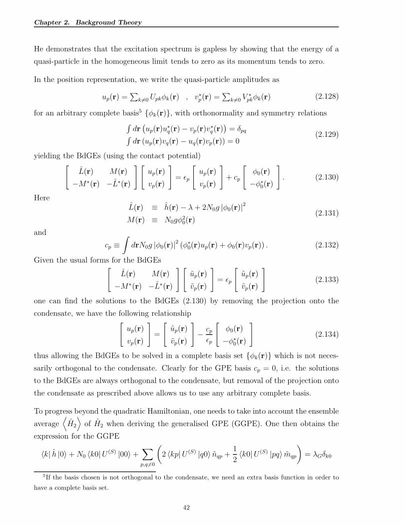
Chapter 2. Background Theory
He demonstrates that the excitation spectrum is gapless by showing that the energy of a
quasi-particle in the homogeneous limit tends to zero as its momentum tends to zero.
In the position representation, we write the quasi-particle amplitudes as
up(r) =∑
k 6=0 Upkφk(r) , v∗p(r) =∑
k 6=0 V∗pkφk(r) (2.128)
for an arbitrary complete basis5 φk(r), with orthonormality and symmetry relations∫
dr(
up(r)u∗q(r)− vp(r)v
∗q (r)
)
= δpq∫
dr (up(r)vq(r)− uq(r)vp(r)) = 0(2.129)
yielding the BdGEs (using the contact potential)[
L(r) M(r)
−M∗(r) −L∗(r)
][
up(r)
vp(r)
]
= ǫp
[
up(r)
vp(r)
]
+ cp
[
φ0(r)
−φ∗0(r)
]
. (2.130)
HereL(r) ≡ h(r)− λ+ 2N0g |φ0(r)|2
M(r) ≡ N0gφ20(r)
(2.131)
and
cp ≡∫
drN0g |φ0(r)|2 (φ∗0(r)up(r) + φ0(r)vp(r)) . (2.132)
Given the usual forms for the BdGEs[
L(r) M(r)
−M∗(r) −L∗(r)
][
up(r)
vp(r)
]
= ǫp
[
up(r)
vp(r)
]
(2.133)
one can find the solutions to the BdGEs (2.130) by removing the projection onto the
condensate, we have the following relationship[
up(r)
vp(r)
]
=
[
up(r)
vp(r)
]
− cpǫp
[
φ0(r)
−φ∗0(r)
]
(2.134)
thus allowing the BdGEs to be solved in a complete basis set φk(r) which is not neces-
sarily orthogonal to the condensate. Clearly for the GPE basis cp = 0, i.e. the solutions
to the BdGEs are always orthogonal to the condensate, but removal of the projection onto
the condensate as prescribed above allows us to use any arbitrary complete basis.
To progress beyond the quadratic Hamiltonian, one needs to take into account the ensemble
average⟨
H2
⟩
of H2 when deriving the generalised GPE (GGPE). One then obtains the
expression for the GGPE
〈k| h |0〉+N0 〈k0|U (S) |00〉+∑
p,q 6=0
(
2 〈kp|U (S) |q0〉 nqp +1
2〈k0|U (S) |pq〉 mqp
)
= λGδk0
5If the basis chosen is not orthogonal to the condensate, we need an extra basis function in order to
have a complete basis set.
42
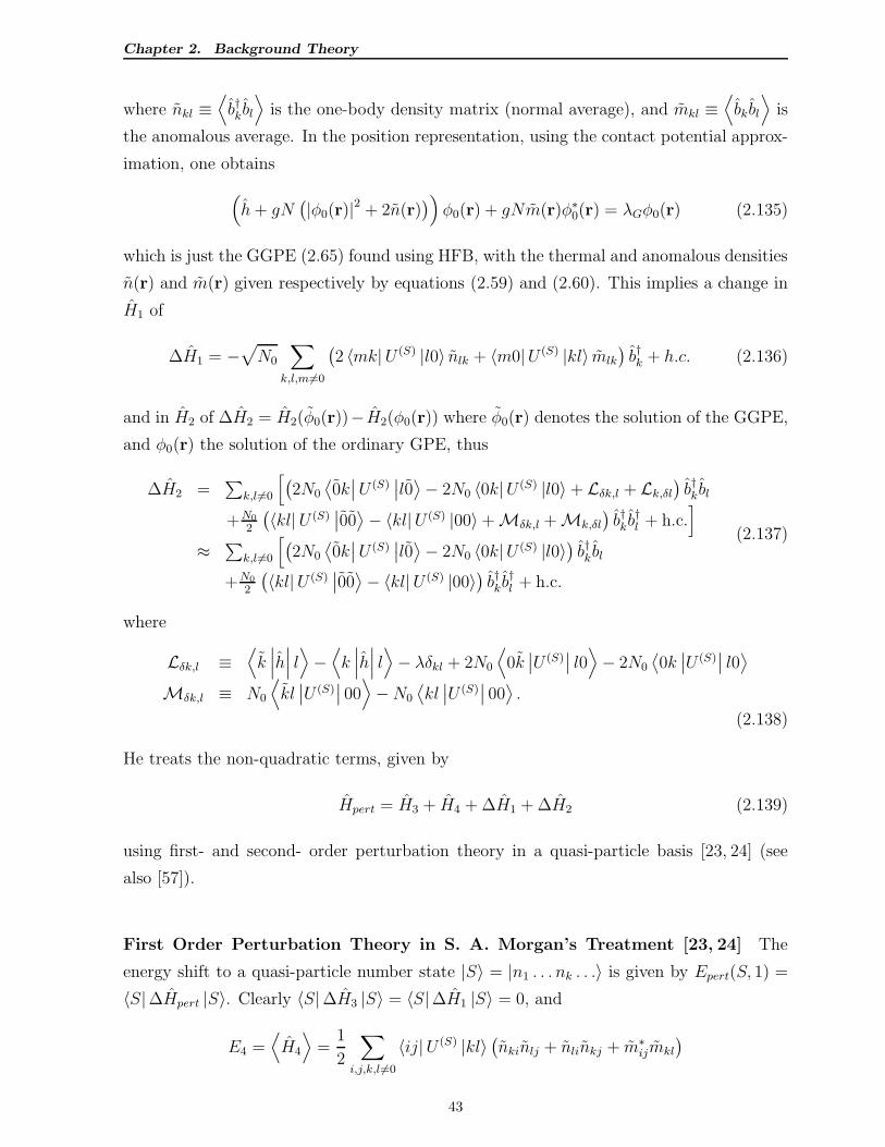
Chapter 2. Background Theory
where nkl ≡⟨
b†k bl
⟩
is the one-body density matrix (normal average), and mkl ≡⟨
bk bl
⟩
is
the anomalous average. In the position representation, using the contact potential approx-
imation, one obtains
(
h+ gN(
|φ0(r)|2 + 2n(r))
)
φ0(r) + gNm(r)φ∗0(r) = λGφ0(r) (2.135)
which is just the GGPE (2.65) found using HFB, with the thermal and anomalous densities
n(r) and m(r) given respectively by equations (2.59) and (2.60). This implies a change in
H1 of
∆H1 = −√
N0
∑
k,l,m6=0
(
2 〈mk|U (S) |l0〉 nlk + 〈m0|U (S) |kl〉 mlk
)
b†k + h.c. (2.136)
and in H2 of ∆H2 = H2(φ0(r))− H2(φ0(r)) where φ0(r) denotes the solution of the GGPE,
and φ0(r) the solution of the ordinary GPE, thus
∆H2 =∑
k,l 6=0
[
(
2N0
⟨
0k∣
∣U (S)∣
∣l0⟩
− 2N0 〈0k|U (S) |l0〉+ Lδk,l + Lk,δl
)
b†k bl
+N0
2
(
〈kl|U (S)∣
∣00⟩
− 〈kl|U (S) |00〉+Mδk,l +Mk,δl
)
b†k b†l + h.c.
]
≈ ∑
k,l 6=0
[
(
2N0
⟨
0k∣
∣U (S)∣
∣l0⟩
− 2N0 〈0k|U (S) |l0〉)
b†k bl
+N0
2
(
〈kl|U (S)∣
∣00⟩
− 〈kl|U (S) |00〉)
b†k b†l + h.c.
(2.137)
where
Lδk,l ≡⟨
k∣
∣
∣h∣
∣
∣l⟩
−⟨
k∣
∣
∣h∣
∣
∣l⟩
− λδkl + 2N0
⟨
0k∣
∣U (S)∣
∣ l0⟩
− 2N0
⟨
0k∣
∣U (S)∣
∣ l0⟩
Mδk,l ≡ N0
⟨
kl∣
∣U (S)∣
∣ 00⟩
−N0
⟨
kl∣
∣U (S)∣
∣ 00⟩
.
(2.138)
He treats the non-quadratic terms, given by
Hpert = H3 + H4 + ∆H1 + ∆H2 (2.139)
using first- and second- order perturbation theory in a quasi-particle basis [23, 24] (see
also [57]).
First Order Perturbation Theory in S. A. Morgan’s Treatment [23, 24] The
energy shift to a quasi-particle number state |S〉 = |n1 . . . nk . . .〉 is given by Epert(S, 1) =
〈S|∆Hpert |S〉. Clearly 〈S|∆H3 |S〉 = 〈S|∆H1 |S〉 = 0, and
E4 =⟨
H4
⟩
=1
2
∑
i,j,k,l 6=0
〈ij|U (S) |kl〉(
nkinlj + nlinkj + m∗ijmkl
)
43
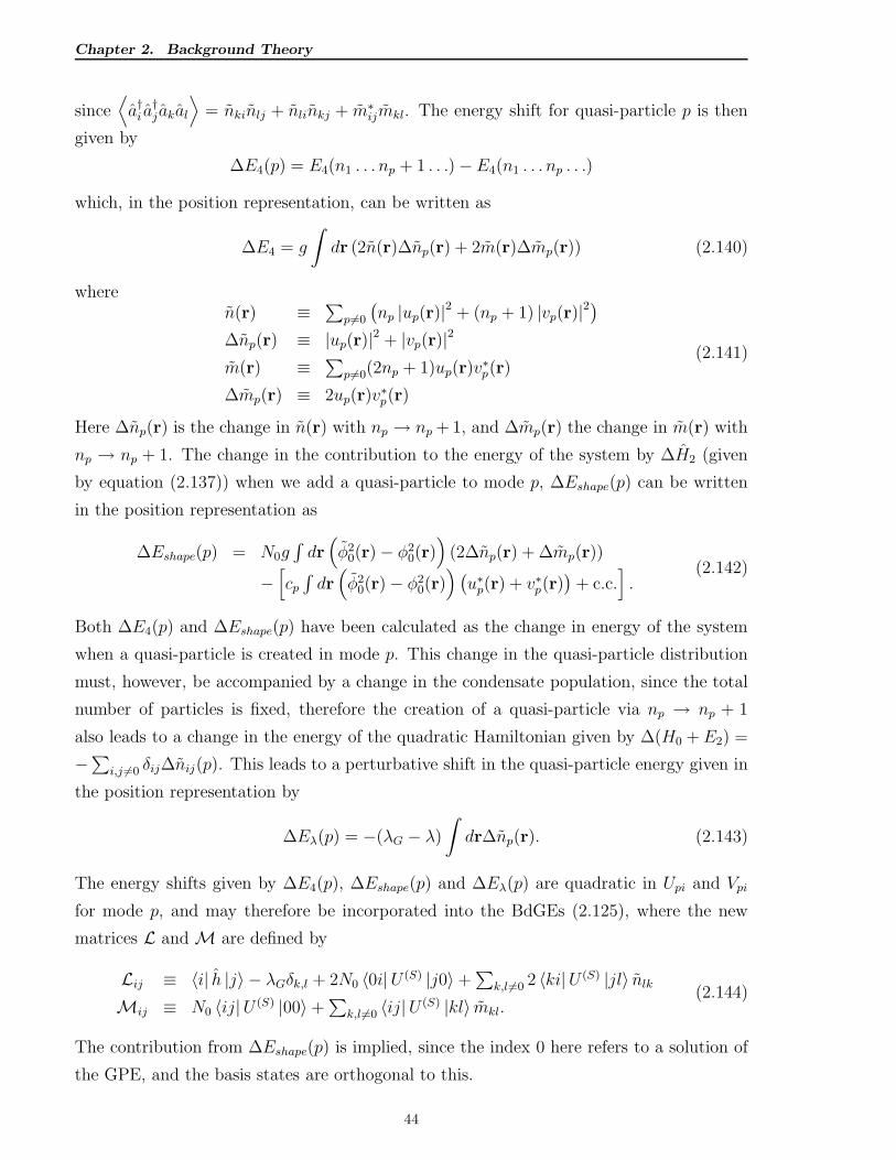
Chapter 2. Background Theory
since⟨
a†i a†j akal
⟩
= nkinlj + nlinkj + m∗ijmkl. The energy shift for quasi-particle p is then
given by
∆E4(p) = E4(n1 . . . np + 1 . . .)−E4(n1 . . . np . . .)
which, in the position representation, can be written as
∆E4 = g
∫
dr (2n(r)∆np(r) + 2m(r)∆mp(r)) (2.140)
wheren(r) ≡
∑
p 6=0
(
np |up(r)|2 + (np + 1) |vp(r)|2)
∆np(r) ≡ |up(r)|2 + |vp(r)|2
m(r) ≡∑
p 6=0(2np + 1)up(r)v∗p(r)
∆mp(r) ≡ 2up(r)v∗p(r)
(2.141)
Here ∆np(r) is the change in n(r) with np → np + 1, and ∆mp(r) the change in m(r) with
np → np + 1. The change in the contribution to the energy of the system by ∆H2 (given
by equation (2.137)) when we add a quasi-particle to mode p, ∆Eshape(p) can be written
in the position representation as
∆Eshape(p) = N0g∫
dr(
φ20(r)− φ2
0(r))
(2∆np(r) + ∆mp(r))
−[
cp∫
dr(
φ20(r)− φ2
0(r))
(
u∗p(r) + v∗p(r))
+ c.c.]
.(2.142)
Both ∆E4(p) and ∆Eshape(p) have been calculated as the change in energy of the system
when a quasi-particle is created in mode p. This change in the quasi-particle distribution
must, however, be accompanied by a change in the condensate population, since the total
number of particles is fixed, therefore the creation of a quasi-particle via np → np + 1
also leads to a change in the energy of the quadratic Hamiltonian given by ∆(H0 +E2) =
−∑
i,j 6=0 δij∆nij(p). This leads to a perturbative shift in the quasi-particle energy given in
the position representation by
∆Eλ(p) = −(λG − λ)
∫
dr∆np(r). (2.143)
The energy shifts given by ∆E4(p), ∆Eshape(p) and ∆Eλ(p) are quadratic in Upi and Vpi
for mode p, and may therefore be incorporated into the BdGEs (2.125), where the new
matrices L andM are defined by
Lij ≡ 〈i| h |j〉 − λGδk,l + 2N0 〈0i|U (S) |j0〉+∑
k,l 6=0 2 〈ki|U (S) |jl〉 nlk
Mij ≡ N0 〈ij|U (S) |00〉+∑
k,l 6=0 〈ij|U (S) |kl〉 mkl.(2.144)
The contribution from ∆Eshape(p) is implied, since the index 0 here refers to a solution of
the GPE, and the basis states are orthogonal to this.
44
Chapter 2. Background Theory
Ordinary perturbation amounts to the simple evaluation of the expressions for ∆E4(p),
∆Eshape(p) and ∆Eλ(p) using quasi-particle energies, and transformation coefficients cal-
culated from the quadratic BdGEs (i.e. ordinary BdGEs where Lij = 〈i| h |j〉 − λδk,l +
2N0 〈0i|U (S) |j0〉 andMij = N0 〈ij|U (S) |00〉 ). Self-consistent perturbation theory, on the
other hand, entails the exact diagonalisation of the generalised BdGEs with Lij and Mij
as above. Comparison of the normal Lij andMij with the generalised Lij andMij shows
that there are three types of correction introduced by ∆E4(p), ∆Eshape(p) and ∆Eλ(p):
1. Condensate energy λ and shape φ0(r) are upgraded to values appropriate to GGPE
2. Direct and exchange collisions are included between non-condensate atoms and via
the term∑
k,l 6=0 2 〈ki|U (S) |jl〉 nlk in Lij
3. The anomalous average mij is introduced into the off-diagonal terms Mij. We can
interpret this correction as follows:- it upgrades the condensate-condensate interac-
tions which appear in leading order contribution toMij so that these are described
by the many-body T-matrix.
We note that the change to coefficients Lij and Mij which are introduced by ∆E4(p) are
exactly the same as would have been obtained using the factorisation approximation used
in HFB on the operators appearing in H4. Hence this approximation on the product of four
operators is equivalent to self-consistent first-order perturbation theory, and is therefore
justified to this order of calculation. Wick’s Theorem is concerned with operator averages,
and hence the equations from first-order perturbation theory and HFB are identical - this
follows since by Wick’s theorem, all ensemble averages of terms having an odd number of
fluctuation creation and annihilation operators η† and η are zero, whereas those with an
even number may be evaluated yielding the same terms.
Second Order Perturbation Theory in S. A. Morgan’s Treatment [23, 24] The
energy shift of a quasi-particle state |S〉 from second order perturbation theory is
Epert(S, 2) =∑
R6=S
∣
∣
∣〈R| Hpert |S〉
∣
∣
∣
2
ES −ER(2.145)
where ES and ER are energies of the system calculated from the quadratic Hamiltonian.
45
Chapter 2. Background Theory
One can neglect the contribution from H4 +∆H2 at this order of perturbation theory, thus
we need only consider the modified cubic Hamiltonian H ′3 = H3 + ∆H1. We can write
H ′3 = H3 + ∆H1 =
[
∑
i,j,k 6=0
(
Aijkaiaj ak +Bijkai†aj ak
)
+∑
i6=0
Ciai
]
+ h.c. (2.146)
where
Aijk =√
N0
∑
m,n,q 6=0
〈q0|U (S) |mn〉ViqUjnUkm + 〈mn|U (S) |q0〉UiqVjnVkm (2.147)
Bijk =√N0
∑
m,n,q 6=0
[
〈q0|U (S) |mn〉(
U∗iqUjnUkm + V ∗
inVjqUkm + V ∗imUjnVkm
)
+ 〈mn|U (S) |q0〉(
U∗inUjqVkm + U∗
imVjnUkq + V ∗iqVjnVkm
)] (2.148)
and
Ci = −∑
q 6=0
(Bqqi +Bqiq)nq (2.149)
The modified cubic Hamiltonian gives a contribution to the energy of
E3 = 16
∑
i,j,k 6=0
∣
∣AP3ijk
∣
∣
2(ninjnk − (ni + 1)(nj + 1)(nk + 1)) /(ǫi + ǫj + ǫk)
+12
∑
i,j,k 6=0 |Bijk +Bikj|2 ((ni + 1)njnk − ni(nj + 1)(nk + 1)) /(ǫj + ǫk − ǫi)−∑i6=0
∣
∣
∣Ci +
∑
j (Bjji +Bjij)nj
∣
∣
∣
2
/ǫi
(2.150)
where AP3ijk ≡ Aijk + Aikj + Ajik + Ajki + Akij + Akji (omitting terms which are negligible
in the thermodynamic limit). The contribution to the energy of a quasi-particle is given
by the change in E3 as np → np + 1, ∆E3(p) = E3(n1 . . . np + 1 . . .) − E3(n1 . . . np . . .),
hence [23, 24]
∆E3(p) =∑
i,j 6=0
[
−∣
∣AP3pij
∣
∣
2(1 + ni + nj)
2(ǫp + ǫi + ǫj)+|Bpij +Bpji|2 (1 + ni + nj)
2(ǫp − ǫi − ǫj)+|Bijp +Bipj |2 (nj − ni)
(ǫp − ǫi + ǫj)
]
.
(2.151)
Although this expresson has been derived for pure states, it may be re-interpreted as
a thermal average. Thermal averages are calculated via the grand canonical partition
function Zc =∑
ni exp (−βEini), where Eini = H0ni + E2ni. To a good ap-
proximation, however, they can be obtained simply by replacing the condensate and quasi-
particle populations with their thermal averages given by the Bose-Einstein distribution
np(T ) = 1/ (Z−1 exp (βǫp)− 1) with fugacity Z ≡ exp (β(µ− λ)), where µ is the chemical
potential.
The physical interpretation of ∆E3(p) is that it introduces a T-matrix into the descrip-
tion of the condensate-non-condensate collisions. The first term in the above equation
46
Chapter 2. Background Theory
corresponds to the simultaneous annihilation or creation of three quasi-particles. The
second term represents Beliaev processes in which a single quasi-particle spontaneously
decomposes into two others. The final term corresponds to Landau processes in which two
quasi-particles collide and coaelesce to form a single quasi-particle (essentially the reverse
of a Beliaev process). Beliaev processes can occur at zero temperature, and are found to
be dominant in the low temperature regime, whereas Landau processes cannot occur at
zero temperature (because there are no excited quasi-particles at zero temperature), but
dominate at high temperatures. The existence of these processes implies that the quasi-
particles have a finite life-time. ∆E3(p) can be used for a trapped gas to calculate the
time evolution of a quasi-particle, and to determine its lifetime. We note that ∆E3(p) is a
quadratic form in the quasi-particle transformation coefficients Upi and Vpi for mode p.
We can write ∆E3(p) in the form
∆E3(p) =[
up −v∗p
]
[
∆L(ǫp) ∆M(ǫp)
−∆M∗(−ǫp) −∆L∗(−ǫp)
][
up
vp
]
(2.152)
where
∆Lij(ǫp) =∑
k,m6=0
[
1 + nk + nm
2
(
AikmA∗jkm
ǫp − (ǫk + ǫm)− B∗
ikmBjkm
ǫp + ǫk + ǫm
)
+ (nm − nk)C∗
ikmC∗jkm
ǫp + ǫm − ǫk
]
(2.153)
and
∆Mij(ǫp) =∑
k,m6=0
[
1 + nk + nm
2
(
AikmB∗jkm
ǫp − (ǫk + ǫm)− B∗
ikmAjkm
ǫp + ǫk + ǫm
)
+ (nm − nk)C∗
ikmC∗jkm
ǫp + ǫm − ǫk
]
(2.154)
where, in the position representation using the contact potential approximation
Aikm = 2√N0g
∫
drφ∗i (r) [φ∗
0(r)uk(r)um(r) + φ0(r) (uk(r)vm(r) + vk(r)um(r))]
Bikm = 2√N0g
∫
drφi(r) [φ0(r)vk(r)vm(r) + φ∗0(r) (uk(r)vm(r) + vk(r)um(r))]
Cikm = 2√N0g
∫
drφi(r) [φ0(r)u∗k(r)vm(r) + φ∗
0(r) (u∗k(r)um(r) + v∗k(r)vm(r))] .
(2.155)
We note that ∆L∗ji(ǫp) = ∆Lij(ǫp), and ∆Mji(ǫp) = ∆Mij(−ǫp).
Since ∆E3(p) simply modifies the matrices L andM in the BdGEs (2.125), its calculation
can be made self-consistent by including ∆L(ǫp) and ∆M(ǫp) in the BdGEs, and calculat-
ing them exactly. Including also the effects of ∆E4(p), ∆Eshape(p) and ∆Eλ(p), he obtains
the generalised BdGEs[
L(ǫp) M(ǫp)
−M∗(−ǫp) −L∗(−ǫp)
][
up
vp
]
= ǫp
[
up
vp
]
(2.156)
47
Chapter 2. Background Theory
where L(ǫp) andM(ǫp) are the matrices with elements
Lij(ǫp) = Lij + ∆Lij(ǫp) and Mij(ǫp) =Mij + ∆Mij(ǫp) (2.157)
with
Lij ≡ 〈i| h |j〉 − λδk,l + 2N0 〈0i|U (S) |j0〉+∑
k,l 6=0 2 〈ki|U (S) |jl〉 nlk
Mij ≡ N0 〈ij|U (S) |00〉+∑
k,l 6=0 〈ij|U (S) |kl〉 mkl
(2.158)
We note the following:
1. The matrix to be diagonalised now depends on the quasi-particle energy, therefore a
single matrix diagonalisation no longer yields the whole quasi-particle spectrum.
2. The factorisation approximation neglects all Beliaev and Landau processes which
can occur in the non-condensate. These give a contribution to the energy of the
order of ∆E4(p) but neglect terms in ∆E3(p) since by Wick’s theorem ensemble
averages for terms involving an odd number of the fluctuation operators η and η†
are identically zero. Therefore the factorisation approximation results in inconsistent
treatment of the non-quadratic Hamiltonian, and hence ∆E3(p) is required to remove
IR divergences in the theory, leading to a gapless spectrum.
Applicability The formalism of S. A. Morgan [23, 24] is directly applicable to the cal-
culation of energy shifts using second-order perturbation theory to take into account the
Beliaev and Landau processes. The disadvantage of this approach is that the generalised
BdGEs (2.156) are difficult to solve and are quite computationally intensive. The other
problem is that dynamic shifts in the quasi-particle energies are not taken into account,
the reason being that the thermal density is static and therefore introduces an effective
potential which modifies the energy shifts - for example, one would not expect Kohn’s
theorem6 to be rigorously satisfied for the m = 1 mode. Rather one would expect the
m = 1 mode frequency to be under-estimated by a few percent for T ∼ Tc/2, depending
on the interaction strength in the BEC.
This formalism is strictly time-independent in view of the way the energy shifts are intro-
duced into the BdGEs (2.125) using the form (2.152) for the quasi-particle energy shifts.
Therefore this formalism is not compatible with any time-dependent theory. In chapter 4
6Kohn’s theorem states that for a harmonically trapped BEC, the dipole mode of the condensate
(corresponding to the centre of mass oscillation), should occur at the harmonic oscillator frequency (see,
for example, the review article [5]).
48
Chapter 2. Background Theory
we shall explore an adaptation of this theory which uses the same expression (2.151) for
the quasi-particle energy shifts, but which is also consistent with a time-dependent theory
in which the condensate and thermal populations are always orthogonal.
The Approach due to Y. Castin and R. Dum
In their paper [25], Castin and Dum argue along the lines that in the case of the U(1)
symmetry-breaking approach, the state of the system is described by a coherent state,
hence the atomic field operator has a non-zero expectation value ( [66], see also [22]).
The mean value is thus a classical field characterising the condensate, and constitutes
an explicit U(1) symmetry-breaking as the condensate has a well-defined phase. But it
should be noted that a coherent state is not a stationary state of the system since it does
not have a well-defined number of particles. The Bogoliubov approach [67, 68] predicts
a time divergence of quantum phase fluctuations. We can interpret this as a quantum
phase spreading of the condensate which invalidates the linearization around the classical
field very soon (as the number of particles is small). In their approach, Y. Castin and R.
Dum [25] do not rely on symmetry-breaking, and thus avoid pathologies associated with
phase fluctuations of the condensate. In their analysis, they use the contact potential
approximation U(r1 − r2) = gδ(r1 − r2) where g = 4π~2as/m and where as is the s-wave
scattering length, as already described.
The condensate wave-function [69] is described as the expectation value of the trace of the
one-body density matrix ρ1(r, r, t) =⟨
ψ†(r, t)ψ(r, t)⟩
where the one-body density matrix
is given by
ρ1(r, r′, t) = 〈r| ρ1(t) |r′〉 =
⟨
ψ†(r, t)ψ(r′, t)⟩
(2.159)
for the field operator ψ(r, t) in the Heisenberg picture. They assume that the number
of particles N is well-defined (so Tr(ρ1) = N) and suppose an N -particle system that is
initially in thermal equilibrium at temperature T . A condensate is present if ρ1 has an
eigenvector |φ〉 with eigenvalue Nc of the order of N , far exceeding all other eigenvalues,
i.e. ρ1 |φ〉 = Nc |φ〉. The condensate wave-function |φ〉 is the exact state in which a
macroscopic number Nc of particles is condensed. Clearly |φ〉 is normalised to unity, ie.
〈φ| φ〉 =∫
dr |φ(r)|2 = 1. We are thus justified in splitting the field operator ψ(r, t) into a
condensate part (macroscopic matrix elements), and a non-condensate part (accounts for
non-condensed particles)
ψ(r, t) = φ(r, t)ac(t) + η(r, t) (2.160)
49
Chapter 2. Background Theory
where the condensate mode operator is given by
ac(t) =
∫
drφ∗(r, t)ψ(r, t) (2.161)
with φ(r, t) normalised to unity, i.e.
∫
dr |φ(r, t)|2 = 1. (2.162)
In the Schrodinger picture ac(t) annihilates a particle in the condensate (wave-function
φ(r, t)). Furthermore, ac(t) has matrix elements of the order of√Nc since the expectation
value⟨
a†c(t)ac(t)⟩
= Nc.
The non-condensate part η(r, t) is obtained by the projection of the field operator ψ(r, t)
orthogonally to φ(r, t) :
η(r, t) =
∫
dr′ 〈r| Q(t) |r′〉 ψ(r′, t) =
∫
dr′Q(r, r′, t)ψ(r′, t) (2.163)
where the projection operator Q(t) = 1 − |φ〉 〈φ| projects onto the one-particle states or-
thogonal to the condensate wave-function φ. In the position representation, the projection
operator Q(t) may be written as
Q(r, r′, t) = δ(r− r′)− φ(r, t)φ∗(r′, t) (2.164)
Clearly η(r, t) is orthogonal to φ(r, t) since∫
drφ∗η =∫
drφ∗ ∫ dr′Q(r, r′, t)ψ(r′, t) =∫
drφ∗ψ −(∫
drφ∗φ) ∫
drφ∗ψ = 0 by the normalisation condition (2.162). Furthermore
(2.163) shows that η(r, t) satisfies the quasi-bosonic commutation relations
[
η(r, t), η†(r′, t)]
= Q(r, r′, t) (2.165)
From (2.160), (2.161), and (2.162), we see that η(r, t) commutes with a†c(t), i.e.
[
a†c(t), η(r, t)]
= 0. (2.166)
They now write the Hamiltonian as a systematic expansion in powers of N−1/2 and identify
a small parameter by introducing the operator
Λ(r, t) =1√
Na†c(t)η(r, t) (2.167)
where N is the total number operator. This has validity in the regime where the mean
number of non-condensed atoms is very much less than the total number of atoms. In this
50
Chapter 2. Background Theory
regime one can identify
√
⟨
ˆδN⟩
/N as the small parameter, where⟨
ˆδN⟩
≡∫
dr⟨
η†η⟩
≪
NC ≈ N. They expand Λ(r, t) and φ(r, t) in powers of 1/√
N :
Λ(r, t) = Λ(0)(r, t) +1√
NΛ(1)(r, t) +
1
NΛ(2)(r, t) + . . . (2.168)
and
φ(r, t) = φ(0)(r, t) +1√
Nφ(1)(r, t) +
1
Nφ(2)(r, t) + . . . (2.169)
Then, performing the asymptotic expansion in the limit of large N (noting the implicit
factor of N in these expansions, see [25] for more details), they find to various orders of
N1/2:
Order N1/2: The Gross-Pitaevskii Equation Consideration of terms of order N1/2
yields the time-dependent Gross-Pitaevskii equation (GPE)(
−i~ ∂∂t
+ HGP (r, t)
)
φ(0)(r, t) = ξ(t)φ(0)(r, t) (2.170)
where the arbitrary real function ξ(t) corresponds to an arbitrary global phase of the
wave-function φ(0)(r, t). The last term in the one-particle Hamiltonian7 HGP (r, t), namely
gN
∣
∣φ(0)(r, t)∣
∣
2) describes an effective mean-field potential due to particle interactions. In
steady state, the one-body density matrix ρ1 is time-independent, and φ(0) can also be
chosen to be time-independent, so the GPE reduces to
HGP (r)∣
∣φ(0)⟩
= µ∣
∣φ(0)⟩
(2.171)
where ξ(t) = µ is a constant determined from the normalisation of φ(0) to unity. µ, then,
represents the lowest-order approximation for the chemical potential of the system. When
solving the time-dependent GPE, we usually take the solution of HGP (r)∣
∣φ(0)⟩
= µ∣
∣φ(0)⟩
as the initial condition, with ξ(t = 0) = µ, in particular.
Order N0: The Time-dependent Bogoliubov-de Gennes Equations To order N0,
one obtains the equation for the BdGEs
i~ ∂∂t
Λ(r, t) =(
h(r, t)− ξ(t))
Λ(r, t) + gN
∫
dr′dr′′Q(r, r′, t)Q(r′, r′′, t) |φ(r′′, t)|2 Λ(r′′, t)
+gN
∫
dr′dr′′Q(r, r′, t)Q∗(r′, r′′, t)φ2(r′′, t)Λ†(r′′, t)
(2.172)
7This is the one-particle Gross-Pitaevskii Hamiltonian, and contains both kinetic and potential energy
terms.
51
Chapter 2. Background Theory
which can be re-writen in operator notation as
i~∂
∂t
[
Λ(r, t)
Λ†(r, t)
]
= L(t) [
Λ(r, t)
Λ†(r, t)
]
(2.173)
where
L(t) ≡[
h+ gNQ(t) |φ(r, t)|2 Q(t)− ξ(t) gNQ(t)φ2(r, t)Q∗(t)
−gNQ∗(t)φ∗2
(r, t)Q(t) −h∗ + gNQ∗(t) |φ(r, t)|2 Q∗(t) + ξ(t)
]
(2.174)
with O Ψ ≡∫
dr′O |r′〉 Ψ(r′) and hence O Ψ(r) ≡∫
dr′ 〈r| O |r′〉 Ψ(r′) and where, for
example, we note that [65]
(
Q(t) |φ(r, t)|2 Q(t))
Λ(r, t) ≡∫
dr′∫
dr′′Q(r, r′, t)Q(r′, r′′, t) |φ(r′′, t)|2 Λ(r′′, t).
(2.175)
Order N−1/2- Corrections to the Gross-Pitaevskii Equation To order N−1/2 the
corrections to the Gross-Pitaevskii equation are zero.
Order N−1- Corrections to the Gross-Pitaevskii Equation To order N−1, one finds
for the component orthogonal φ(2)⊥ (r′, t) to φ(0)(r′, t)
−i~ ∂∂tφ
(2)⊥ (r, t) =
(
h(r, t)− ξ(t))
φ(2)⊥ (r, t) + gN
∫
dr′dr′′Q(r, r′, t)Q(r′, r′′, t) |φ(r′′, t)|2 φ(2)⊥ (r′′, t)
+gN
∫
dr′dr′′Q(r, r′, t)Q(r′, r′′, t)φ2(r′′, t)φ(2)∗
⊥ (r′′, t)
−gN
∫
dr′Q(r, r′, t)[
|φ(r′, t)|2 φ(r′, t)(
1 +∫
dr′′n(r′′, r′′, t))]
+gN
∫
dr′Q(r, r′, t) [2n(r′, r′, t)φ(r′, t) + m(r′, r′, t)φ∗(r′, t)]
−gN
∫
dr′dr′′Q(r, r′, t) |φ(r′′, t)|2 [n(r′′, r′, t)φ(r′′, t) + m(r′′, r′, t)φ∗(r′′, t)] .
(2.176)
They interpret the above equation as follows:
1. The term−gN
∫
dr′Q(r, r′, t)[
|φ(r′, t)|2 φ(r′, t)(
1 +∫
dr′′n(r′′, r′′, t))]
corrects the over-
estimation of the number of condensed particles in calculating their mutual interac-
tions N → N −(
1 +⟨
ˆδN⟩)
in the GPE.
2. The term gN
∫
dr′Q(r, r′, t) [2n(r′, r′, t)φ(r′, t) + m(r′, r′, t)φ∗(r′, t)] describes the in-
teraction of the condensed particles and the non-condensed ones - we can understand
this in terms of the mean-field picture - the Hartree-Fock approximation.
3. The term−gN
∫
dr′dr′′Q(r, r′, t) |φ(r′′, t)|2 [n(r′′, r′, t)φ(r′′, t) + m(r′′, r′, t)φ∗(r′′, t)] cor-
responds to the spatial correlation of the non-condensed particles.
52
Chapter 2. Background Theory
One can choose the component φ(2)‖ (r, t) along φ(0)(r, t) arbitrarily, using the arbitrariness
of the global phase of φ(r, t) .
The time-evolution of Λ They show that the time evolution of the operators Λ (i.e. the
dynamics of the non-condensed particles) amounts to propating a perturbation orthogonal
to φ. They choose a basis which diagonalises L at time t = 0 given by the Bogoliubov
transformation
Λ(r, t) =∑
k
(
uk(r, t)ak + v∗k(r, t)a†k
)
(2.177)
where the usual Bose commutation relations (2.45)
[
ak, a†l
]
= δkl and [ak, al] =[
a†k, a†l
]
= 0
apply. They show the equivalence of the quantum fluctuations described by Λ and the
time-evolution of small perturbations δφ of the time-dependent solution of the GPE using
linear-response theory.
Applicability The formalism of Castin and Dum hasn’t been used as such - Morgan et.
al. [60] used linear response theory based on the GGPE (2.84). A systematic expansion
approach is used here, so the theory can be extended to higher orders. The order of
difficulty is of the same order as that used by Morgan et. al. [60]. The time-dependent
formalism, however, is not applicable, because angular momentum conservation is violated
- see comments towards bottom of page 89, chapter 4.
The Approach due to S. A. Gardiner et. al.
In their treatment of the time-dependent problem, S. A. Gardiner et. al. [26] follow closely
along the lines of the analysis by Castin and Dum [25]. As in [25], they split the Bose field
operator ψ(r, t) in the Hamiltonian (2.18) subject to the contact potential approximation
U(r) = gδ(r), i.e. Eq. (2.24)
H(t) =
∫
dr(
ψ†(r, t)h(r)ψ(r, t) +g
2ψ†(r, t)ψ†(r, t)ψ(r, t)ψ(r, t)
)
into a condensate part (macroscopic matrix elements), and a non-condensate part (ac-
counting for the remaining non-condensate particles) (2.160)
ψ(r, t) = φ(r, t)ac(t) + η(r, t)
53
Chapter 2. Background Theory
where φ(r, t) is normalised to unity. This is justified in the presence of a condensate in
view of the fact that there is one distinct eigenfunction φ(r, t) with unit normalisation that
has a corresponding eigenvalue Nc(t) that is much larger than all the other eigenvalues, i.e.
∫
dr′ρ(r, r′, t)φ(r′, t) = Nc(t)φ(r, t) (2.178)
where ρ(r, r′, t) = 〈ρ(r, r′, t)〉 =⟨
ψ†(r, t)ψ(r′, t)⟩
is the single-particle density matrix.
They differ in their choice of fluctuation operator from Castin and Dum [25], preferring
the choice (c.f. Eq. (2.167))
Λ(r, t) =1
√
Nc(t)a†c(t)η(r, t) (2.179)
with commutation relation
[
Λ(r, t), Λ†(r′, t)]
=Nc(t)
Nc(t)Q(r, r′, t)− 1
Nc(t)η†(r′, t)η(r, t) (2.180)
where we have defined (2.164)
Q(r, r′, t) ≡ δ(r− r′)− φ(r, t)φ∗(r′, t)
for the following reasons:
1. Λ(r, t) scales as√
Nt(t). The fluctuation operator Λ(r, t) = 1√Na†c(t)η(r, t) as used
by Castin and Dum [25] scales as√
Nc(t)Nt(t)/N ≈√
Nt(t) and therefore scales
satisfactorily only when Nc(t) ≈ N , hence requiring that the fluctuations are small
compared to the square root of the number of condensed particles. The scaling used
here, however, is not dependent on the requirement that Nc(t) ≈ N .
2. To the order of the calculation used here the commutation relation,[
Λ(r, t), Λ†(r′, t)]
may be taken to be Q(r, r′, t).
They note that
Nc(t)−Nc(t) =∫
dr⟨
η†(r, t)η(r, t)⟩
−∫
drη†(r, t)η(r, t)
=∫
dr⟨
Λ†(r, t)Nc(t)
Nc(t)Λ(r, t)
⟩
−∫
drˆ(r, t)Nc(t)
Nc(t)Λ(r, t)
≈∫
dr⟨
Λ†(r, t)Λ(r, t)⟩
−∫
drΛ†(r, t)Λ(r, t)
to quadratic order in Λ(r, t) (which is sufficient for the level of approximation used here).
Substituting the placement (2.160) and the expression (2.179) for the fluctuation operator
54
Chapter 2. Background Theory
in the Hamiltonian (2.24), and applying the Gaussian approximation of the fluctuation
terms
Λ†(r, t)Λ(r, t)Λ(r, t) ≈ 2⟨
Λ†(r, t)Λ(r, t)⟩
Λ(r, t) +⟨
Λ(r, t)Λ(r, t)⟩
Λ†(r, t) (2.181)
they finally obtain the Hamiltonian H(3)(t) to cubic order (denoted by the superscript (3))
given by
H(3)(t) = NcH(3)0 (t) +
√
NcH(3)1 (t) + H
(3)2 (t) +
1√Nc
H(3)3 (t) (2.182)
where
H(3)0 (t) =
∫
drφ∗(
h +gNc
2|φ|2)
φ (2.183)
H(3)1 (t) =
∫
dr[
φ∗(
h+ gNc |φ|2)
Λ + h.c.]
(2.184)
H(3)2 (t) =
∫
dr[
Λ†(
h + 2gNc |φ|2)
Λ +(
12gNcφ
∗2ΛΛ + h.c.
)
− 12gNc |φ|4
]
+[
∫
dr(⟨
Λ†Λ⟩
− Λ†Λ)]
∫
drφ∗(
h+ gNc |φ|2)
φ(2.185)
and
H(3)3 (t) =
∫
dr
φ∗[
2⟨
Λ†Λ⟩
Λ +⟨
ΛΛ⟩
Λ†]
+ h.c.
− gNc
∫
dr[
φ∗ |φ|2 Λ + h.c.]
+∫
drdr′
φ∗(r, t) |φ(r, t)|2[⟨
Λ†(r′, t)Λ(r, t)⟩
Λ(r′, t) + h.c.
+⟨
Λ(r′, t)Λ(r, t)⟩
Λ†(r′, t) + h.c.]
.
(2.186)
Then assuming that the bosonic field operator has no explicit time dependence, they obtain
to various orders of approximation:
Order N1/2c - The Gross-Pitaevskii Equation Considering terms in H(3)(t) to order
N1/2c (i.e. terms H
(3)0 (t) and H
(3)1 (t)) yields the time-dependent Gross-Pitaevskii equation
i~∂φ(r, t)
∂t=(
h(r, t) + gNc |φ(r, t)|2 − λ0
)
φ(r, t) (2.187)
where
λ0 =
∫
drφ∗(r, t)
(
h(r, t) + gNc |φ(r, t)|2 − i~∂φ(r, t)
∂t
)
φ(r, t) (2.188)
(c.f. Castin and Dum [25]) which, in the time-independent case, reduces to
λ0φ(r) =(
h(r) + gNc |φ(r)|2)
φ(r) (2.189)
where λ0 is an eigenvalue of this equation corresponding to the chemical potential.
55
Chapter 2. Background Theory
Order N0c - The Modified Bogoliubov de-Gennes Equations They find to order
N0c the generalised BdGEs given by
i~∂Λ(r, t)
∂t=(
h+ gNc |φ|2 − λ0
)
Λ(r, t)+gNc
∫
dr′Q(r, r′, t)[
|φ(r′, t)|2 Λ(r′, t) + φ2(r′, t)Λ†(r′, t)]
.
(2.190)
Order N−1/2c - The Generalised Gross-Pitaevskii Equation They find to order
N−1/2c the GGPE
i~ ∂∂tφ(r, t) =
(
h + gNc
[(
1− 1Nc
)
|φ|2 + 2Nc
⟨
Λ†Λ⟩]
− λ2
)
φ(r, t) + g⟨
ΛΛ⟩
φ∗(r, t)
−g∫
dr′ |φ(r′, t)|2[⟨
Λ†(r′, t)Λ(r, t)⟩
φ(r′, t) +⟨
Λ(r′, t)Λ(r, t)⟩
φ∗(r′, t)]
.
(2.191)
The GGPE (2.191) and the modified BdGEs (2.190) describe the second-order coupled
condensate and non-condensate dynamics, and constitute the main result of the paper [26].
In the quasi-particle basis, using the Bogoliubov transformation
Λ(r, t) =∑
k
(
uk(r, t)ak + v∗k(r, t)a†k
)
(2.192)
the modified BdGEs become
i~ ∂∂t
[
uq(r, t)
vq(r, t)
]
=∫
dr′
[
L(r, r′, t) M(r, r′, t)
−M∗(r, r′, t) −L∗(r, r′, t)
][
uq(r′, t)
vq(r′, t)
]
(2.193)
where we have defined
L(r, r′, t) ≡ δ(r, r′)(
h(r) + gNc |φ(r, t)|2 − λ0
)
+ gNc
∫
dr′′Q(r, r′′, t)Q(r′′, r′, t) |φ(r′, t)|2
(2.194)
and
M(r, r′, t) ≡ gNc
∫
dr′′Q(r, r′′, t)Q(r′′, r′, t)φ2(r′, t) (2.195)
and define the densities
n(r′, r, t) ≡⟨
Λ†(r′, t)Λ(r, t)⟩
, n(r, t) ≡⟨
Λ†(r, t)Λ(r, t)⟩
m(r′, r, t) ≡⟨
Λ(r′, t)Λ(r, t)⟩
, m(r, t) ≡⟨
Λ(r, t)Λ(r, t)⟩ (2.196)
Here
n(r, t) ≡⟨
η†(r, t)η(r, t)⟩
=∑
q
[
|uq(r, t)|2NBE(ǫq) + |vq(r, t)|2 (NBE(ǫq) + 1)]
56
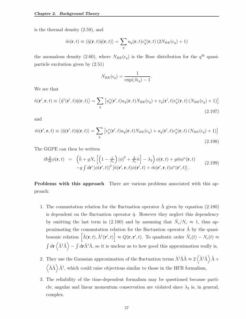
Chapter 2. Background Theory
is the thermal density (2.59), and
m(r, t) ≡ 〈η(r, t)η(r, t)〉 =∑
q
uq(r, t)v∗q(r, t) (2NBE(ǫq) + 1)
the anomalous density (2.60), where NBE(ǫq) is the Bose distribution for the qth quasi-
particle excitation given by (2.51)
NBE(ǫq) =1
exp(βǫq)− 1.
We see that
n(r′, r, t) ≡⟨
η†(r′, t)η(r, t)⟩
=∑
q
[
u∗q(r′, t)uq(r, t)NBE(ǫq) + vq(r
′, t)v∗q (r, t) (NBE(ǫq) + 1)]
(2.197)
and
m(r′, r, t) ≡ 〈η(r′, t)η(r, t)〉 =∑
q
[
v∗q (r′, t)uq(r, t)NBE(ǫq) + uq(r
′, t)v∗q (r, t) (NBE(ǫq) + 1)]
(2.198)
The GGPE can then be written
i~ ∂∂tφ(r, t) =
(
h+ gNc
[(
1− 1Nc
)
|φ|2 + 2Ncn]
− λ2
)
φ(r, t) + gmφ∗(r, t)
−g∫
dr′ |φ(r′, t)|2 [n(r′, r, t)φ(r′, t) + m(r′, r, t)φ∗(r′, t)] .(2.199)
Problems with this approach There are various problems associated with this ap-
proach:
1. The commutation relation for the fluctuation operator Λ given by equation (2.180)
is dependent on the fluctuation operator η. However they neglect this dependency
by omitting the last term in (2.180) and by assuming that Nc/Nc ≈ 1, thus ap-
proximating the commutation relation for the fluctuation operator Λ by the quasi-
bosonic relation[
Λ(r, t), Λ†(r′, t)]
≈ Q(r, r′, t). To quadratic order Nc(t) − Nc(t) ≈∫
dr⟨
Λ†Λ⟩
−∫
drΛ†Λ, so it is unclear as to how good this approximation really is,
2. They use the Gaussian approximation of the fluctuation terms Λ†ΛΛ ≈ 2⟨
Λ†Λ⟩
Λ +⟨
ΛΛ⟩
Λ†, which could raise objections similar to those in the HFB formalism,
3. The reliability of the time-dependent formalism may be questioned because parti-
cle, angular and linear momentum conservation are violated since λ2 is, in general,
complex.
57
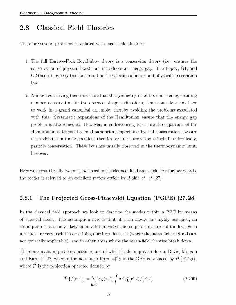
Chapter 2. Background Theory
2.8 Classical Field Theories
There are several problems associated with mean field theories:
1. The full Hartree-Fock Bogoliubov theory is a conserving theory (i.e. ensures the
conservation of physical laws), but introduces an energy gap. The Popov, G1, and
G2 theories remedy this, but result in the violation of important physical conservation
laws.
2. Number conserving theories ensure that the symmetry is not broken, thereby ensuring
number conservation in the absence of approximations, hence one does not have
to work in a grand canonical ensemble, thereby avoiding the problems associated
with this. Systematic expansions of the Hamiltonian ensure that the energy gap
problem is also remedied. However, in endeavouring to ensure the expansion of the
Hamiltonian in terms of a small parameter, important physical conservation laws are
often violated in time-dependent theories for finite size systems including, ironically,
particle conservation. These laws are usually observed in the thermodynamic limit,
however.
Here we discuss briefly two methods used in the classical field approach. For further details,
the reader is referred to an excellent review article by Blakie et. al. [27].
2.8.1 The Projected Gross-Pitaevskii Equation (PGPE) [27,28]
In the classical field approach we look to describe the modes within a BEC by means
of classical fields. The assumption here is that all such modes are highly occupied, an
assumption that is only likely to be valid provided the temperatures are not too low. Such
methods are very useful in describing quasi-condensates (where the mean-field methods are
not generally applicable), and in other areas where the mean-field theories break down.
There are many approaches possible, one of which is the approach due to Davis, Morgan
and Burnett [28] wherein the non-linear term |φ|2 φ in the GPE is replaced by P
|φ|2 φ
,
where P is the projection operator defined by
P f(r, t) =∑
k∈C
φk(r, t)
∫
dr′φ∗k(r
′, t)f(r′, t) (2.200)
58
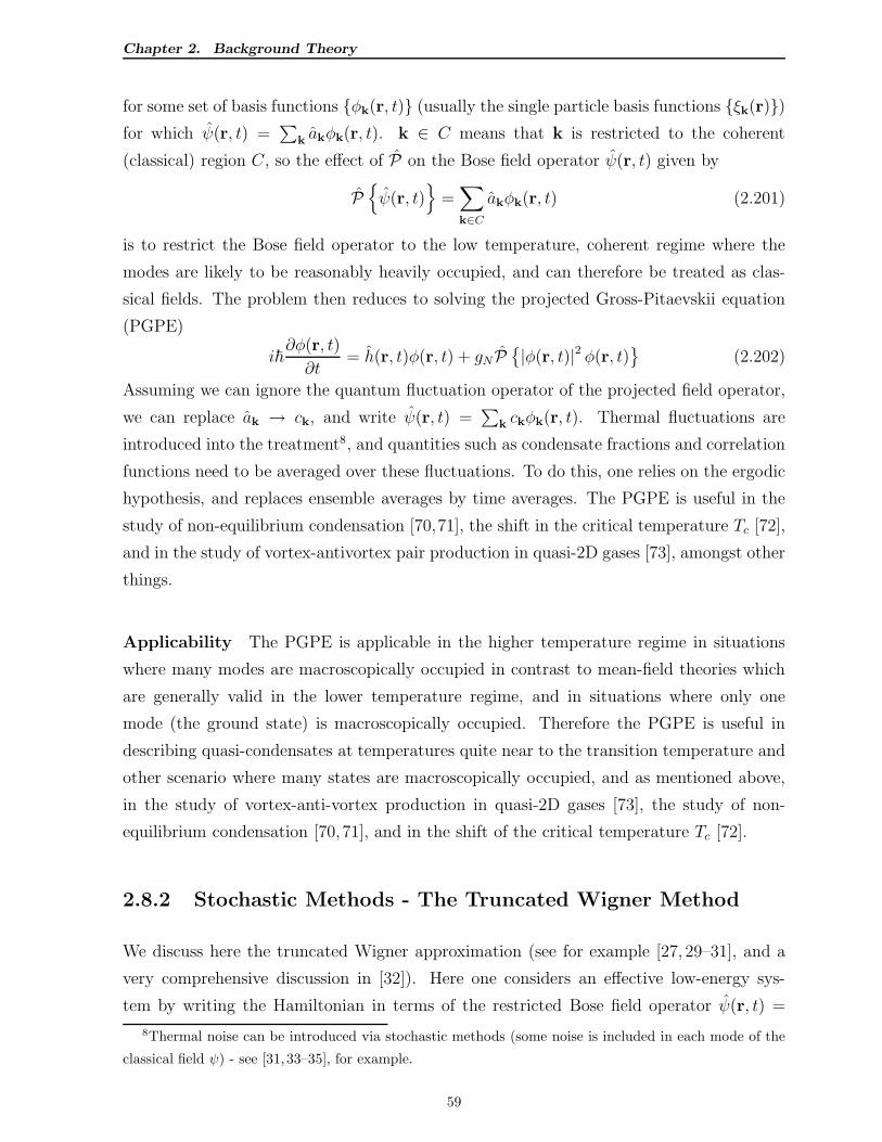
Chapter 2. Background Theory
for some set of basis functions φk(r, t) (usually the single particle basis functions ξk(r))for which ψ(r, t) =
∑
kakφk(r, t). k ∈ C means that k is restricted to the coherent
(classical) region C, so the effect of P on the Bose field operator ψ(r, t) given by
P
ψ(r, t)
=∑
k∈C
akφk(r, t) (2.201)
is to restrict the Bose field operator to the low temperature, coherent regime where the
modes are likely to be reasonably heavily occupied, and can therefore be treated as clas-
sical fields. The problem then reduces to solving the projected Gross-Pitaevskii equation
(PGPE)
i~∂φ(r, t)
∂t= h(r, t)φ(r, t) + gN P
|φ(r, t)|2 φ(r, t)
(2.202)
Assuming we can ignore the quantum fluctuation operator of the projected field operator,
we can replace ak → ck, and write ψ(r, t) =∑
k ckφk(r, t). Thermal fluctuations are
introduced into the treatment8, and quantities such as condensate fractions and correlation
functions need to be averaged over these fluctuations. To do this, one relies on the ergodic
hypothesis, and replaces ensemble averages by time averages. The PGPE is useful in the
study of non-equilibrium condensation [70,71], the shift in the critical temperature Tc [72],
and in the study of vortex-antivortex pair production in quasi-2D gases [73], amongst other
things.
Applicability The PGPE is applicable in the higher temperature regime in situations
where many modes are macroscopically occupied in contrast to mean-field theories which
are generally valid in the lower temperature regime, and in situations where only one
mode (the ground state) is macroscopically occupied. Therefore the PGPE is useful in
describing quasi-condensates at temperatures quite near to the transition temperature and
other scenario where many states are macroscopically occupied, and as mentioned above,
in the study of vortex-anti-vortex production in quasi-2D gases [73], the study of non-
equilibrium condensation [70, 71], and in the shift of the critical temperature Tc [72].
2.8.2 Stochastic Methods - The Truncated Wigner Method
We discuss here the truncated Wigner approximation (see for example [27, 29–31], and a
very comprehensive discussion in [32]). Here one considers an effective low-energy sys-
tem by writing the Hamiltonian in terms of the restricted Bose field operator ψ(r, t) =
8Thermal noise can be introduced via stochastic methods (some noise is included in each mode of the
classical field ψ) - see [31, 33–35], for example.
59
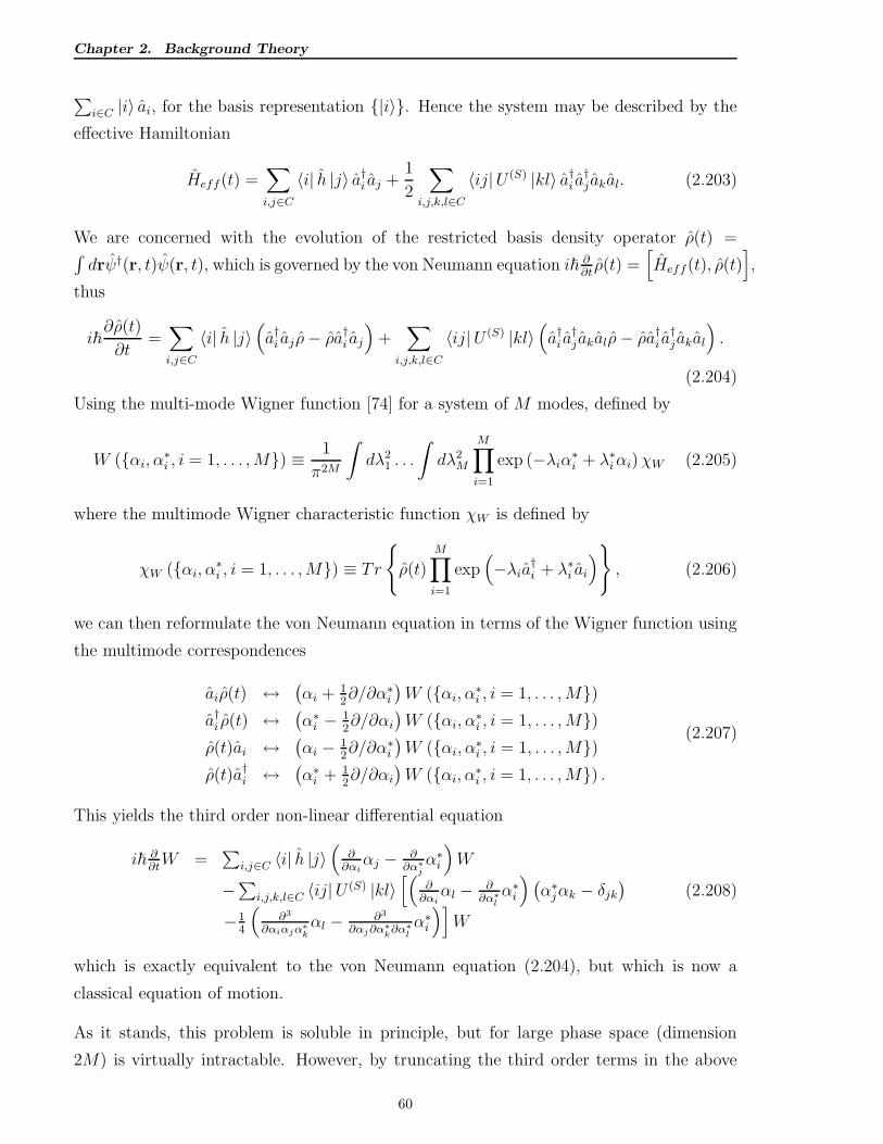
Chapter 2. Background Theory
∑
i∈C |i〉 ai, for the basis representation |i〉. Hence the system may be described by the
effective Hamiltonian
Heff(t) =∑
i,j∈C
〈i| h |j〉 a†i aj +1
2
∑
i,j,k,l∈C
〈ij|U (S) |kl〉 a†i a†j akal. (2.203)
We are concerned with the evolution of the restricted basis density operator ρ(t) =∫
drψ†(r, t)ψ(r, t), which is governed by the von Neumann equation i~ ∂∂tρ(t) =
[
Heff(t), ρ(t)]
,
thus
i~∂ρ(t)
∂t=∑
i,j∈C
〈i| h |j〉(
a†i aj ρ− ρa†i aj
)
+∑
i,j,k,l∈C
〈ij|U (S) |kl〉(
a†i a†j akalρ− ρa†i a†j akal
)
.
(2.204)
Using the multi-mode Wigner function [74] for a system of M modes, defined by
W (αi, α∗i , i = 1, . . . ,M) ≡ 1
π2M
∫
dλ21 . . .
∫
dλ2M
M∏
i=1
exp (−λiα∗i + λ∗iαi)χW (2.205)
where the multimode Wigner characteristic function χW is defined by
χW (αi, α∗i , i = 1, . . . ,M) ≡ Tr
ρ(t)
M∏
i=1
exp(
−λia†i + λ∗i ai
)
, (2.206)
we can then reformulate the von Neumann equation in terms of the Wigner function using
the multimode correspondences
aiρ(t) ↔(
αi + 12∂/∂α∗
i
)
W (αi, α∗i , i = 1, . . . ,M)
a†i ρ(t) ↔(
α∗i − 1
2∂/∂αi
)
W (αi, α∗i , i = 1, . . . ,M)
ρ(t)ai ↔(
αi − 12∂/∂α∗
i
)
W (αi, α∗i , i = 1, . . . ,M)
ρ(t)a†i ↔(
α∗i + 1
2∂/∂αi
)
W (αi, α∗i , i = 1, . . . ,M) .
(2.207)
This yields the third order non-linear differential equation
i~ ∂∂tW =
∑
i,j∈C 〈i| h |j〉(
∂∂αiαj − ∂
∂α∗jα∗
i
)
W
−∑i,j,k,l∈C 〈ij|U (S) |kl〉[(
∂∂αiαl − ∂
∂α∗l
α∗i
)
(
α∗jαk − δjk
)
−14
(
∂3
∂αiαjα∗k
αl − ∂3
∂αj∂α∗k∂α∗
l
α∗i
)]
W
(2.208)
which is exactly equivalent to the von Neumann equation (2.204), but which is now a
classical equation of motion.
As it stands, this problem is soluble in principle, but for large phase space (dimension
2M) is virtually intractable. However, by truncating the third order terms in the above
60
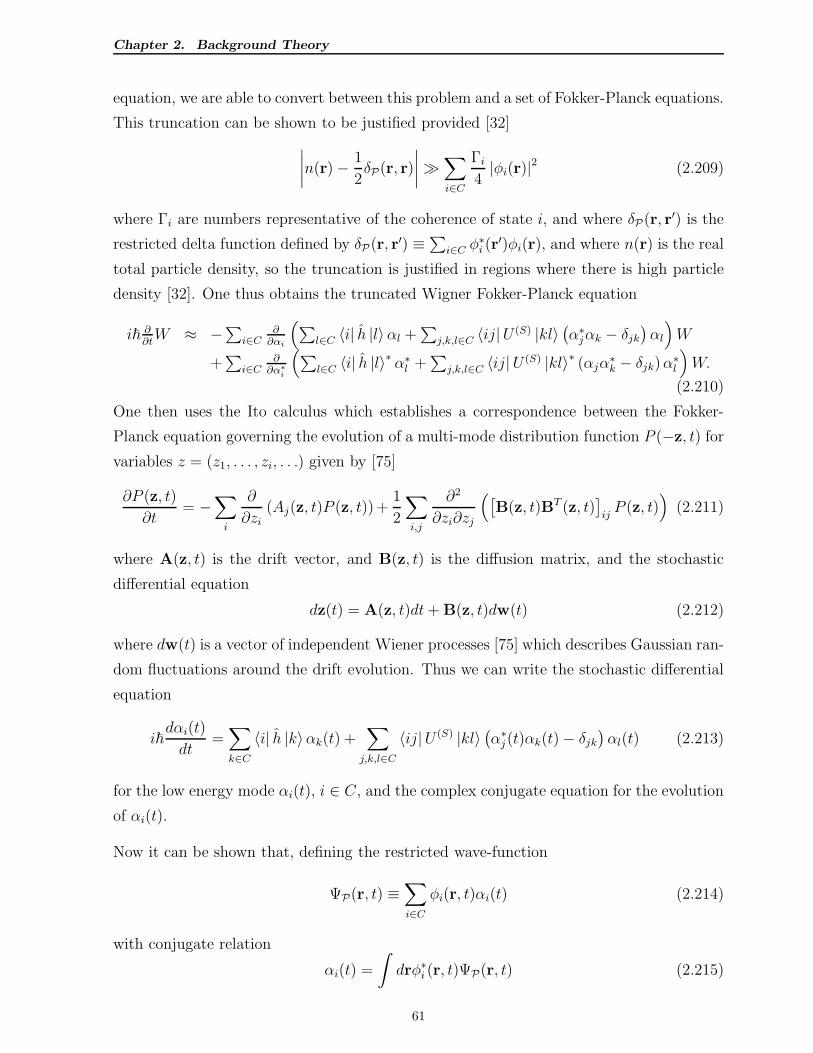
Chapter 2. Background Theory
equation, we are able to convert between this problem and a set of Fokker-Planck equations.
This truncation can be shown to be justified provided [32]
∣
∣
∣
∣
n(r)− 1
2δP(r, r)
∣
∣
∣
∣
≫∑
i∈C
Γi
4|φi(r)|2 (2.209)
where Γi are numbers representative of the coherence of state i, and where δP(r, r′) is the
restricted delta function defined by δP(r, r′) ≡∑
i∈C φ∗i (r
′)φi(r), and where n(r) is the real
total particle density, so the truncation is justified in regions where there is high particle
density [32]. One thus obtains the truncated Wigner Fokker-Planck equation
i~ ∂∂tW ≈ −
∑
i∈C∂
∂αi
(
∑
l∈C 〈i| h |l〉αl +∑
j,k,l∈C 〈ij|U (S) |kl〉(
α∗jαk − δjk
)
αl
)
W
+∑
i∈C∂
∂α∗i
(
∑
l∈C 〈i| h |l〉∗ α∗
l +∑
j,k,l∈C 〈ij|U (S) |kl〉∗ (αjα∗k − δjk)α∗
l
)
W.
(2.210)
One then uses the Ito calculus which establishes a correspondence between the Fokker-
Planck equation governing the evolution of a multi-mode distribution function P (−z, t) for
variables z = (z1, . . . , zi, . . .) given by [75]
∂P (z, t)
∂t= −
∑
i
∂
∂zi(Aj(z, t)P (z, t))+
1
2
∑
i,j
∂2
∂zi∂zj
(
[
B(z, t)BT (z, t)]
ijP (z, t)
)
(2.211)
where A(z, t) is the drift vector, and B(z, t) is the diffusion matrix, and the stochastic
differential equation
dz(t) = A(z, t)dt+ B(z, t)dw(t) (2.212)
where dw(t) is a vector of independent Wiener processes [75] which describes Gaussian ran-
dom fluctuations around the drift evolution. Thus we can write the stochastic differential
equation
i~dαi(t)
dt=∑
k∈C
〈i| h |k〉αk(t) +∑
j,k,l∈C
〈ij|U (S) |kl〉(
α∗j (t)αk(t)− δjk
)
αl(t) (2.213)
for the low energy mode αi(t), i ∈ C, and the complex conjugate equation for the evolution
of αi(t).
Now it can be shown that, defining the restricted wave-function
ΨP(r, t) ≡∑
i∈C
φi(r, t)αi(t) (2.214)
with conjugate relation
αi(t) =
∫
drφ∗i (r, t)ΨP(r, t) (2.215)
61
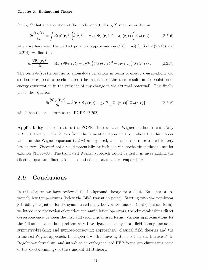
Chapter 2. Background Theory
for i ∈ C that the evolution of the mode amplitudes αi(t) may be written as
i~∂αi(t)
∂t=
∫
drφ∗(r, t)[
h(r, t) + gN
(
|ΨP(r, t)|2 − δP(r, r))
]
ΨP(r, t) (2.216)
where we have used the contact potential approximation U(r) = gδ(r). So by (2.213) and
(2.214), we find that
i~∂ΨP(r, t)
∂t= h(r, t)ΨP(r, t) + gNP
(
|ΨP(r, t)|2 − δP(r, r))
ΨP(r, t)
. (2.217)
The term δP(r, r) gives rise to anomalous behaviour in terms of energy conservation, and
so therefore needs to be eliminated (the inclusion of this term results in the violation of
energy conservation in the presence of any change in the external potential). This finally
yields the equation
i~∂ΨP(r, t)
∂t= h(r, t)ΨP(r, t) + gNP
|ΨP(r, t)|2 ΨP(r, t)
(2.218)
which has the same form as the PGPE (2.202).
Applicability In contrast to the PGPE, the truncated Wigner method is essentially
a T = 0 theory. This follows from the truncation approximation where the third order
terms in the Wigner equation (2.208) are ignored, and hence one is restricted to very
low energy. Thermal noise could potentially be included via stochastic methods - see for
example [31, 33–35]. The truncated Wigner approach would be useful in investigating the
effects of quantum fluctuations in quasi-condensates at low temperature.
2.9 Conclusions
In this chapter we have reviewed the background theory for a dilute Bose gas at ex-
tremely low temperatures (below the BEC transition point). Starting with the non-linear
Schrodinger equation for the symmetrised many-body wave-function (first quantised form),
we introduced the notion of creation and annihilation operators, thereby establishing direct
correspondence between the first and second quantised forms. Various approximations for
the full second-quantised problem were investigated, namely mean field theory (including
symmetry-breaking and number-conserving approaches), classical field theories and the
truncated Wigner approach. In chapter 4 we shall investigate more fully the Hartree-Fock-
Bogoliubov formalism, and introduce an orthogonalised HFB formalism eliminating some
of the short-commings of the standard HFB theory.
62
Chapter 3. Vortices in Bose-Einstein Condensates
Chapter 3
Vortices in Bose-Einstein
Condensates
3.1 Introduction
In this chapter we present a brief survey on vortices in BECs, their stability, and their pre-
cession, touching very briefly on solitons. Bose-Einstein Condensates (BECs) are charac-
terised by the macroscopic occupation of some quantum state, usually the ground state (as
opposed to Fermions, which obey the Pauli exclusion principle). This occurs at sufficiently
low temperatures, and is brought about by the quantum statistical properties of Bosons.
Accompanied by this is associated long-range order of the condensate. Thus one can asso-
ciate with the condensate, an order parameter, which is in this case, the wave function of
the quantum state in question. This is manifest in the coherence of the atoms/molecules
in the condensate population of the BEC. For a stationary BEC, therefore, the condensate
phase is well-defined throughout (apart from topological defects such as vortices which
may be present), except in the case of large fluctuations arising in low-dimensional systems
at relatively high temperatures. The condensate is supposedly a superfluid, which implies
persistent flow, in particular the continued rotation of the fluid in vortices, even when the
source of rotation is removed.
Vortices in fluids result from rotation of the fluid at sufficiently high angular frequencies.
Classically when a fluid is rotated rapidly, a depletion of the fluid at the centre of rotation
results as a consequence of the angular momentum of the fluid due to the rotation. However,
when the source of the rotation is removed, the vortex dissipates and the fluid reverts back
63
Chapter 3. Vortices in Bose-Einstein Condensates
to its lowest energy state, which is absence of rotation.
The situation for a BEC is somewhat different. The BEC is described by an order param-
eter, which is a complex wave function, consisting of an amplitude and a phase. In the
ground state, the phase is uniform throughout. The existence of a phase gradient implies
flow of the condensate. The velocity flow field is proportional to the gradient of the phase.
As a consequence of this, the condensate flow field is irrotational (ie. the velocity field
has curl zero) which implies that vortices, if present, must be quantised. When a phase
singularity occurs anywhere within the BEC, this must necessarily be accompanied by zero
density of the condensate at that point for the wave function to be well-behaved. Such a
phase singularity is known as a topological defect.
Vortices (in two-dimensional systems) and vortex lines (in three-dimensional systems) are
examples of topological defects, and would be accompanied by a non-zero quantum winding
number κ (which, for an axially symmetric trap, coincides with the axial angular momen-
tum quantum number m, an eigensate of the axial angular momentum quantum operator
Lz). In a two-dimensional or three-dimensional BEC, a phase singularity would imply a
circular phase gradient, resulting in a velocity field circulating about the singularity, so the
condensate would tend to flow about this point, resulting in a vortex. There also exists a
region centred on the singularity, called the core of the vortex, where the wave function
amplitude steadily increases as one moves further away from the centre of the core. The
core radius would be roughly that radius at which the amplitude of the wave function
matches the amplitude of the bulk of the condensate. The classical analogue of this would
be a whirlpool. The significant difference is, however, that the flow of a superfluid is ir-
rotational, which rules out, for example, solid body rotation for a single vortex. We can
see this if we consider the example of a BEC in an axially symmetric trap, with a vortex
centered on the axis. A stable normal density mode in this configuration is possible only
if the condensate density is proportional to eimφ, where m is some integer, and φ is the
angle of rotation about the axis. We see that the vortex is quantised with angular quantum
number m, which coincides with the winding quantum number κ, as pointed out earlier.
In the absence of any topological defects, κ = 0 and the macroscopically occupied quantum
state is the ground state with uniform phase. So, for the case of our axially symmetric
system, the BEC in the absence of vortices would be characterised by m = 0. It turns
out that vortices having |m| > 1 are in general unstable (see, for example [79]), since it
would be energetically more favourable for a multi-charged vortex to break up into singly-
charged vortices. So stable vortices would then be characterised by m = ±1, where m = 1
64
Chapter 3. Vortices in Bose-Einstein Condensates
corresponds to a clockwise rotating vortex, and m = −1, an anticlockwise rotating vortex.
In one-dimensional systems, one can impose a phase singularity at a given point, by phase
imprinting, for example. This would be an example of a topological defect in one dimension.
One would expect a topological defect of this type to be the one-dimensional analogue
of the vortex in a two-dimensional system. An example of such a topological defect is
a dark soliton in a 1D BEC with repulsive interactions having velocity zero [8, 76–78].
Such a soliton has a discontinuity in the phase of π at the point of the soliton, and may
therefore be regarded as a 1D topological defect. Solitons (also known as solitary waves) are
localised disturbances which propagate without change of form [8]. This is made possible
in BECs due to the non-linearity of the GPE, where exact solutions can be found in 1D
for homogeneous systems. The subject of solitons is vast (see for example [8, 76–78]), and
will not be presented in this thesis where we shall concentrate more on vortices in quasi-2D
BECs.
3.2 The Theory of Vortices in Bose-Einstein Conden-
sates
The flow in superfluids is dissipationless, so we would expect the rotation associated with a
vortex to be persistent when the source of rotation is removed. It is interesting, therefore,
to investigate whether the theory of BECs leads to this conclusion. The conclusion of the
theory would also need to be tested against experiment.
Much of the earlier theoretical work on the dynamics of vortices (see for example [36–39,79])
assumed T = 0 and neglected the effects of the non-condensate dynamics on the overall
dynamics of the vortex. The stability of vortices is of paramount concern for, as we
pointed out earlier, the persistence of vortices in the absence of the source of rotation is
an important property of superfluids. Rokshar’s work [79] was very important in that it
showed that when the non-condensate dynamics is ignored, a vortex in a harmonic trap is
never locally stable. Rokshar argues that in view of the existence of a state of lower energy
than the condensate state with angular momentum quantum m (which he calls the core
state, which as we shall see later is just the anomalous mode), that it would be energetically
favourable for particles to be transferred from the condensate vortex state to the core state.
This results in the existence of two co-existing condensate states. The resulting many-body
ground state may then be described by the superposition of the vortex condensate state
65
Chapter 3. Vortices in Bose-Einstein Condensates
and the core state [79]
Φ =√
1− xcoreΦm + eiχ√xcoreΦcore (3.1)
where xcore = Ncore/N , Ncore is the number of atoms in the core state, and N is the total
number of atoms.
If the vortex axis is along the z-axis, and the phase angle χ is assumed to be zero (which can
be done without loss of generality), the wave functions Φm and Φcore interfere destructively
off the y-axis and for x > 0. It follows that the vortex core moves off-axis in the x-direction.
Thus Rokshar concludes that the on-centre state can be stable only if the vortex core is
pinned to the centre of the trap by a locally repulsive potential. Rokshar shows that the
variation in energy due to small variations of the axially symmetric vortex wave function
ψ = ψm + δψ is always negative and that therefore the axially symmetric state ψm is not
a local minimum of the energy functional
E
N=
∫
drψ∗(
h+g
2|ψ|2
)
ψ (3.2)
subject to the constraint that ψm ∼ eimφ where (2.22)
h(r) = − ~2
2m∇2
+ VT (r)
and that therefore the on-axis vortex is unstable. Rokshar [79] (see also [80]) shows that
the instability results in a displacement of the vortex, and that Ehrenfest’s theorem implies
precession accompanied by dissipation of the vortex.
Fetter [37] has shown analytically using the GPE for the cases of a rotating uniform
fluid and for a non-uniform rotating fluid with a Thomas-Fermi (TF) profile density
n = n(0)(
1− ρ2
R2
)
for a vortex on the axis of an axially symmetric system, that there
exists critical rotational frequencies Ω0 and ΩCl such that the vortex is in a true equilib-
rium state when the rotational frequency of the fluid Ω ≥ ΩCl (corresponding to the flow
velocity exceeding the Landau critical velocity vLC given by the local speed of sound), and
metastable for Ω0 < Ω < ΩCl. For Ω < Ω0, Fetter shows that the free energy decreases
monotonically with increasing x (distance from axis), so that the vortex spirals outwards
and annihilates with its image vortex (which resides on the boundary of the BEC).
He shows that for Ω > Ω0, the free energy increases monotonically with increasing x,
consequently if the vortex is displaced slightly (but not too much) from the axis, it tends
to return to the axis.
For Ω ≥ ΩCl, the vortex is always stable, and returns to the axis regardless of how large
the displacement.
66
Chapter 3. Vortices in Bose-Einstein Condensates
In a later paper Svidzinsky and Fetter [38] show that a vortex in a trapped BEC has a
mode (the anomalous mode) of positive norm and negative energy (and hence frequency).
This result is for T = 0 and ignores the non-condensate dynamics. This mode is formally
unstable in view of its negative energy. He shows that the negative frequency of the mode
corresponds to the precession of the vortex around the axis of symmetry of the trap, and
that the solution becomes stable above an angular velocity Ω0, characterising the onset
of metastability, (ie. stability with respect to small radial displacements from the central
axis).
Dodd et. al. [39] solved the time independent Bogoliubov equations (T = 0, ignoring
noncondensate dynamics) and found the existence of an eigenvalue having an energy lower
than that of the vortex state Φm(r) (ie. negative energy) implying the instability of the
solution to the Bogoliubov equations for a condensate containing a singly quantised vortex
on the axis. This is identified by Fetter [37] as the so-called anomalous mode. How this
comes about is as follows:
The physical solutions to the BdGEs (2.50) must be consistent with the Bose commutation
relations, which necessitates the normalisation condition (2.54)
∫
dr(
|uq(r, t)|2 − |vq(r, t)|2)
= 1. (3.3)
Consequently only positive norm solutions are physical, ie. those for which
∫
dr(
|uq(r, t)|2 − |vq(r, t)|2)
> 0.
In solving the BdGEs, half the solutions have positive norm, and half negative norm,
so we choose the physical positive norm solutions. When solving the BdGEs for a BEC
in the absence of vortices, all the energies corresponding to the positive norm solutions
are positive (and those corresponding to the negative norm solutions are negative). The
unstable mode that Dodd et. al. [39] found for the singly charged vortex on axis (m = 1)
corresponds to the lowest energy positive norm solution for the quasi-particle energies, and
the energy corresponding to this mode is negative. This is known as the anomalous mode.
Interestingly, the work by Dodd et. al. [39] was originally inspired by the quest for a method
of identifying vortices in an experiment. The method of detection of vortices by current
imaging techniques suffers from the constraint that the viewing of the condensate must
be done in a direction roughly perpendicular to the trap axis. This is due to the magnet
geometries used. Most imaging setups require images of the condensate densities integrated
along the line of sight (as one would logically expect). Clearly it would be desirable to
67
Chapter 3. Vortices in Bose-Einstein Condensates
integrate the density in the plane perpendicular to the trap symmetry axis (also taken to be
the axis of rotation) in order to identify the vortex, but instead the acquired image is along
this plane, so it is difficult to distinguish between a vortex state and the condensed ground
state in this plane. Dodd et. al. [39] showed that the excitation spectum corresponding
to the vortex state would be quite different to that of the the ground state, and hence the
excitation spectroscopy of the vortex line could be used to identify vortices.
Garcia-Ripoll and Perez-Garcia [83] also studied (in 1999) the stability of axially symmet-
ric vortices in trapped gases subject to rotation. They solved the GPE and BdGEs in the
Bogoliubov approximation for a three-dimensional condensate in both the cases of spheri-
cally and cylindrically symmetric traps. Their calculations were done for a wide range of
non-linearity constants of the GPE, ranging from very small values to very large values.
They investigated the stability of vortices for the case of the m = 1 and m = 2 vortex
states, and found that vortices are always energetically unstable for non-rotating systems,
but in the case of the vortex state with m = 1, the vortex can be stabilised by rotation
above a certain critical frequency of rotation, in agreement with the work of Rokshar [79]
and of Fetter et. al. [40]. They found that multi-charged vortices (m = 2 and higher) can
never be energetically stable (a local minimum of the energy functional), and conclude that
the absolute minimum of the energy is not an eigenstate of the Lz operator, even when the
angular frequency of rotation exceeds the critical rotational frequency.
They point out that when a system is unstable in the sense that the BdGEs are unstable,
ie. linear dynamical instability of the linearised system (LS), it is impossible for the system
to be stable in the Lyapunov sense, ie. Lyapunov dynamical stability (LDS) or in the sense
of energetic stability (ES), since
ES⇒ LDS⇒ LS
and so consequently
LS⇒ LDS⇒ ES
As we have seen above, all analyses neglecting the dynamics of the non-condensate led to
the conclusion that below a critical rotational frequency these vortices were unstable and
precessed, dissipating out of the condensate.
In 1999 Isoshima et. al. [2] examined the stabilization of vortices confined by a harmonic
potential by the effect of the non-condensate at finite temperatures, or alternatively, by
an additional pinning potential (eg. a potential produced by a laser beam focussed at the
vortex centre). They solve the time-independent modified GPE (2.81) and BdGEs (2.82)
68
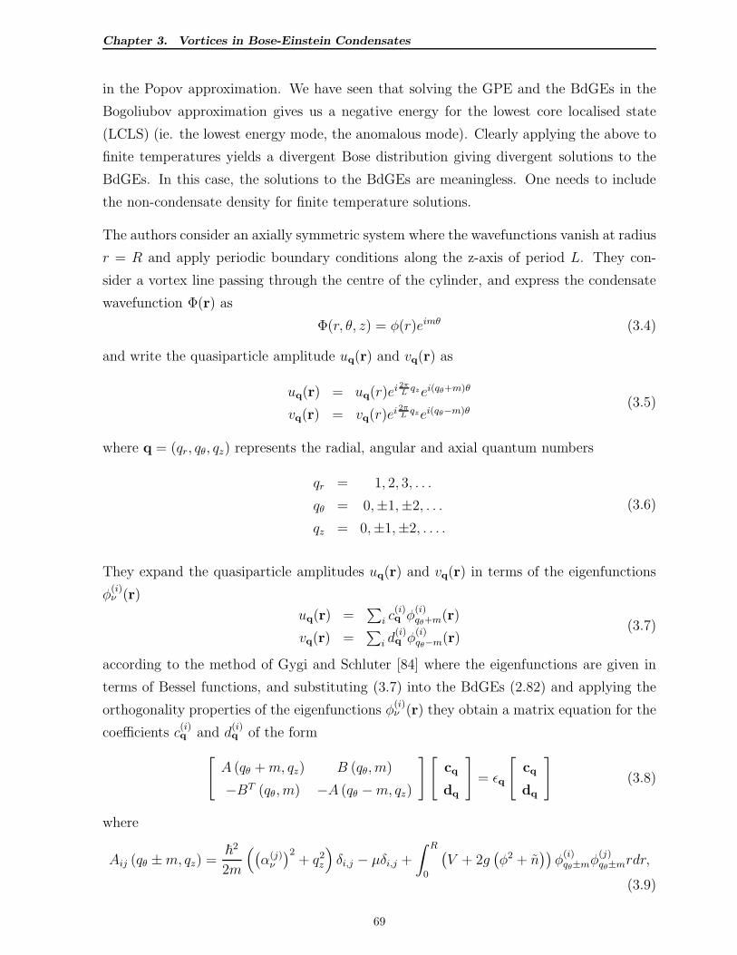
Chapter 3. Vortices in Bose-Einstein Condensates
in the Popov approximation. We have seen that solving the GPE and the BdGEs in the
Bogoliubov approximation gives us a negative energy for the lowest core localised state
(LCLS) (ie. the lowest energy mode, the anomalous mode). Clearly applying the above to
finite temperatures yields a divergent Bose distribution giving divergent solutions to the
BdGEs. In this case, the solutions to the BdGEs are meaningless. One needs to include
the non-condensate density for finite temperature solutions.
The authors consider an axially symmetric system where the wavefunctions vanish at radius
r = R and apply periodic boundary conditions along the z-axis of period L. They con-
sider a vortex line passing through the centre of the cylinder, and express the condensate
wavefunction Φ(r) as
Φ(r, θ, z) = φ(r)eimθ (3.4)
and write the quasiparticle amplitude uq(r) and vq(r) as
uq(r) = uq(r)ei 2π
Lqzei(qθ+m)θ
vq(r) = vq(r)ei 2π
Lqzei(qθ−m)θ
(3.5)
where q = (qr, qθ, qz) represents the radial, angular and axial quantum numbers
qr = 1, 2, 3, . . .
qθ = 0,±1,±2, . . .
qz = 0,±1,±2, . . . .
(3.6)
They expand the quasiparticle amplitudes uq(r) and vq(r) in terms of the eigenfunctions
φ(i)ν (r)
uq(r) =∑
i c(i)q φ
(i)qθ+m(r)
vq(r) =∑
i d(i)q φ
(i)qθ−m(r)
(3.7)
according to the method of Gygi and Schluter [84] where the eigenfunctions are given in
terms of Bessel functions, and substituting (3.7) into the BdGEs (2.82) and applying the
orthogonality properties of the eigenfunctions φ(i)ν (r) they obtain a matrix equation for the
coefficients c(i)q and d
(i)q of the form
[
A (qθ +m, qz) B (qθ, m)
−BT (qθ, m) −A (qθ −m, qz)
][
cq
dq
]
= ǫq
[
cq
dq
]
(3.8)
where
Aij (qθ ±m, qz) =~2
2m
(
(
α(j)ν
)2+ q2
z
)
δi,j − µδi,j +
∫ R
0
(
V + 2g(
φ2 + n))
φ(i)qθ±mφ
(j)qθ±mrdr,
(3.9)
69
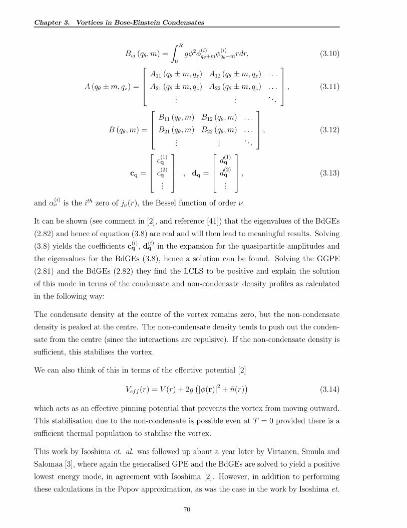
Chapter 3. Vortices in Bose-Einstein Condensates
Bij (qθ, m) =
∫ R
0
gφ2φ(i)qθ+mφ
(i)qθ−mrdr, (3.10)
A (qθ ±m, qz) =
A11 (qθ ±m, qz) A12 (qθ ±m, qz) . . .
A21 (qθ ±m, qz) A22 (qθ ±m, qz) . . ....
.... . .
, (3.11)
B (qθ, m) =
B11 (qθ, m) B12 (qθ, m) . . .
B21 (qθ, m) B22 (qθ, m) . . ....
.... . .
, (3.12)
cq =
c(1)q
c(2)q
...
, dq =
d(1)q
d(2)q
...
, (3.13)
and α(i)ν is the ith zero of jν(r), the Bessel function of order ν.
It can be shown (see comment in [2], and reference [41]) that the eigenvalues of the BdGEs
(2.82) and hence of equation (3.8) are real and will then lead to meaningful results. Solving
(3.8) yields the coefficients c(i)q , d
(i)q in the expansion for the quasiparticle amplitudes and
the eigenvalues for the BdGEs (3.8), hence a solution can be found. Solving the GGPE
(2.81) and the BdGEs (2.82) they find the LCLS to be positive and explain the solution
of this mode in terms of the condensate and non-condensate density profiles as calculated
in the following way:
The condensate density at the centre of the vortex remains zero, but the non-condensate
density is peaked at the centre. The non-condensate density tends to push out the conden-
sate from the centre (since the interactions are repulsive). If the non-condensate density is
sufficient, this stabilises the vortex.
We can also think of this in terms of the effective potential [2]
Veff(r) = V (r) + 2g(
|φ(r)|2 + n(r))
(3.14)
which acts as an effective pinning potential that prevents the vortex from moving outward.
This stabilisation due to the non-condensate is possible even at T = 0 provided there is a
sufficient thermal population to stabilise the vortex.
This work by Isoshima et. al. was followed up about a year later by Virtanen, Simula and
Salomaa [3], where again the generalised GPE and the BdGEs are solved to yield a positive
lowest energy mode, in agreement with Isoshima [2]. However, in addition to performing
these calculations in the Popov approximation, as was the case in the work by Isoshima et.
70
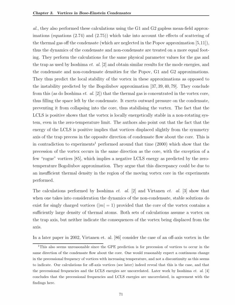
Chapter 3. Vortices in Bose-Einstein Condensates
al., they also performed these calculations using the G1 and G2 gapless mean-field approx-
imations (equations (2.74) and (2.75)) which take into account the effects of scattering of
the thermal gas off the condensate (which are neglected in the Popov approximation [5,11]),
thus the dynamics of the condensate and non-condensate are treated on a more equal foot-
ing. They perform the calculations for the same physical parameter values for the gas and
the trap as used by Isoshima et. al. [2] and obtain similar results for the mode energies, and
the condensate and non-condensate densities for the Popov, G1 and G2 approximations.
They thus predict the local stability of the vortex in these approximations as opposed to
the instability predicted by the Bogoliubov approximation [37, 39, 40, 79]. They conclude
from this (as do Isoshima et. al. [2]) that the thermal gas is concentrated in the vortex core,
thus filling the space left by the condensate. It exerts outward pressure on the condensate,
preventing it from collapsing into the core, thus stabilising the vortex. The fact that the
LCLS is positive shows that the vortex is locally energetically stable in a non-rotating sys-
tem, even in the zero-temperature limit. The authors also point out that the fact that the
energy of the LCLS is positive implies that vortices displaced slightly from the symmetry
axis of the trap precess in the opposite direction of condensate flow about the core. This is
in contradiction to experiments1 performed around that time (2000) which show that the
precession of the vortex occurs in the same direction as the core, with the exception of a
few “rogue” vortices [85], which implies a negative LCLS energy as predicted by the zero-
temperature Bogoliubov approximation. They argue that this discrepancy could be due to
an insufficient thermal density in the region of the moving vortex core in the experiments
performed.
The calculations performed by Isoshima et. al. [2] and Virtanen et. al. [3] show that
when one takes into consideration the dynamics of the non-condensate, stable solutions do
exist for singly charged vortices (|m| = 1) provided that the core of the vortex contains a
sufficiently large density of thermal atoms. Both sets of calculations assume a vortex on
the trap axis, but neither indicate the consequences of the vortex being displaced from the
axis.
In a later paper in 2002, Virtanen et. al. [86] consider the case of an off-axis vortex in the
1This also seems unreasonable since the GPE prediction is for precession of vortices to occur in the
same direction of the condensate flow about the core. One would reasonably expect a continuous change
in the precessional frequency of vortices with increasing temperature, and not a discontinuity as this seems
to indicate. Our calculations for off-axis vortices (see later) indeed reveal that this is the case, and that
the precessional frequencies and the LCLS energies are uncorrelated. Later work by Isoshima et. al. [4]
concludes that the precessional frequencies and LCLS energies are uncorrelated, in agreement with the
findings here.
71
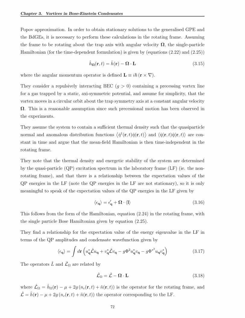
Chapter 3. Vortices in Bose-Einstein Condensates
Popov approximation. In order to obtain stationary solutions to the generalised GPE and
the BdGEs, it is necessary to perform these calculations in the rotating frame. Assuming
the frame to be rotating about the trap axis with angular velocity Ω, the single-particle
Hamiltonian (for the time-dependent formulation) is given by (equations (2.22) and (2.25))
hΩ(r, t) = h(r)−Ω · L (3.15)
where the angular momentum operator is defined L ≡ i~ (r×∇).
They consider a repulsively interacting BEC (g > 0) containing a precessing vortex line
for a gas trapped by a static, axi-symmetric potential, and assume for simplicity, that the
vortex moves in a circular orbit about the trap symmetry axis at a constant angular velocity
Ω. This is a reasonable assumption since such precessional motion has been observed in
the experiments.
They assume the system to contain a sufficient thermal density such that the quasiparticle
normal and anomalous distribution functions⟨
η†(r, t)η(r, t)⟩
and 〈η(r, t)η(r, t)〉 are con-
stant in time and argue that the mean-field Hamiltonian is then time-independent in the
rotating frame.
They note that the thermal density and energetic stability of the system are determined
by the quasi-particle (QP) excitation spectrum in the laboratory frame (LF) (ie. the non-
rotating frame), and that there is a relationship between the expectation values of the
QP energies in the LF (note the QP energies in the LF are not stationary), so it is only
meaningful to speak of the expectation values of the QP energies in the LF given by
〈ǫq〉 = ǫ′q + Ω · 〈l〉 (3.16)
This follows from the form of the Hamiltonian, equation (2.24) in the rotating frame, with
the single particle Bose Hamiltonian given by equation (2.25).
They find a relationship for the expectation value of the energy eigenvalue in the LF in
terms of the QP amplitudes and condensate wavefunction given by
〈ǫq〉 =
∫
dr(
u∗qLuq + v∗qLvq − gΦ2u∗qvq − gΦ∗2
uqv∗q
)
(3.17)
The operators L and LΩ are related by
LΩ = L −Ω · L (3.18)
where LΩ = hΩ(r) − µ + 2g (nc(r, t) + n(r, t)) is the operator for the rotating frame, and
L = h(r)− µ+ 2g (nc(r, t) + n(r, t)) the operator corresponding to the LF.
72
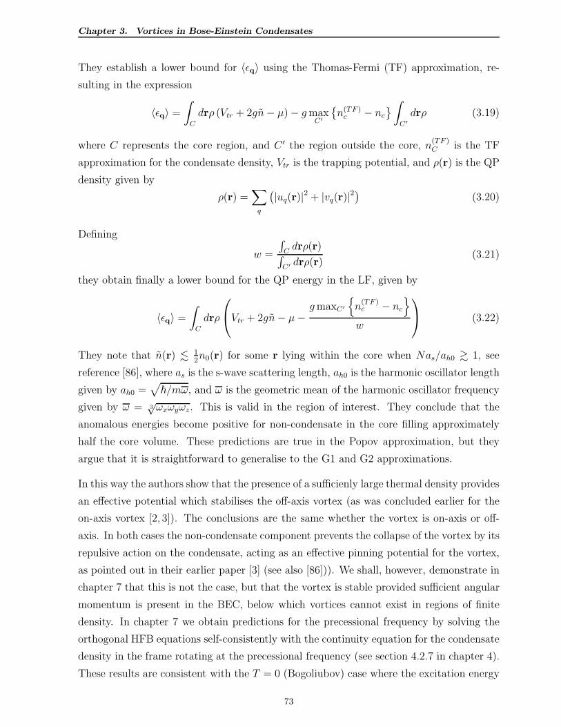
Chapter 3. Vortices in Bose-Einstein Condensates
They establish a lower bound for 〈ǫq〉 using the Thomas-Fermi (TF) approximation, re-
sulting in the expression
〈ǫq〉 =
∫
C
drρ (Vtr + 2gn− µ)− gmaxC′
n(TF )c − nc
∫
C′
drρ (3.19)
where C represents the core region, and C ′ the region outside the core, n(TF )C is the TF
approximation for the condensate density, Vtr is the trapping potential, and ρ(r) is the QP
density given by
ρ(r) =∑
q
(
|uq(r)|2 + |vq(r)|2)
(3.20)
Defining
w =
∫
Cdrρ(r)
∫
C′ drρ(r)(3.21)
they obtain finally a lower bound for the QP energy in the LF, given by
〈ǫq〉 =
∫
C
drρ
Vtr + 2gn− µ−gmaxC′
n(TF )c − nc
w
(3.22)
They note that n(r) . 12n0(r) for some r lying within the core when Nas/ah0 & 1, see
reference [86], where as is the s-wave scattering length, ah0 is the harmonic oscillator length
given by ah0 =√
~/mω, and ω is the geometric mean of the harmonic oscillator frequency
given by ω = 3√ωxωyωz. This is valid in the region of interest. They conclude that the
anomalous energies become positive for non-condensate in the core filling approximately
half the core volume. These predictions are true in the Popov approximation, but they
argue that it is straightforward to generalise to the G1 and G2 approximations.
In this way the authors show that the presence of a sufficienly large thermal density provides
an effective potential which stabilises the off-axis vortex (as was concluded earlier for the
on-axis vortex [2, 3]). The conclusions are the same whether the vortex is on-axis or off-
axis. In both cases the non-condensate component prevents the collapse of the vortex by its
repulsive action on the condensate, acting as an effective pinning potential for the vortex,
as pointed out in their earlier paper [3] (see also [86])). We shall, however, demonstrate in
chapter 7 that this is not the case, but that the vortex is stable provided sufficient angular
momentum is present in the BEC, below which vortices cannot exist in regions of finite
density. In chapter 7 we obtain predictions for the precessional frequency by solving the
orthogonal HFB equations self-consistently with the continuity equation for the condensate
density in the frame rotating at the precessional frequency (see section 4.2.7 in chapter 4).
These results are consistent with the T = 0 (Bogoliubov) case where the excitation energy
73
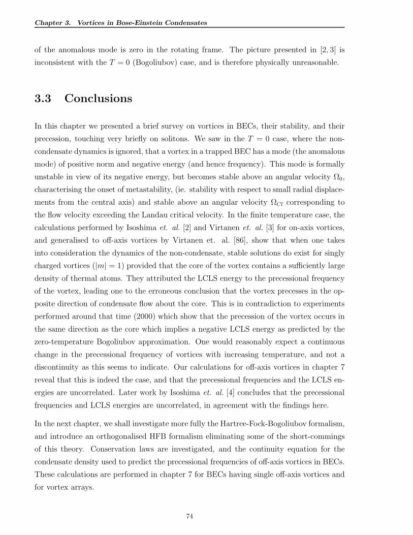
Chapter 3. Vortices in Bose-Einstein Condensates
of the anomalous mode is zero in the rotating frame. The picture presented in [2, 3] is
inconsistent with the T = 0 (Bogoliubov) case, and is therefore physically unreasonable.
3.3 Conclusions
In this chapter we presented a brief survey on vortices in BECs, their stability, and their
precession, touching very briefly on solitons. We saw in the T = 0 case, where the non-
condensate dynamics is ignored, that a vortex in a trapped BEC has a mode (the anomalous
mode) of positive norm and negative energy (and hence frequency). This mode is formally
unstable in view of its negative energy, but becomes stable above an angular velocity Ω0,
characterising the onset of metastability, (ie. stability with respect to small radial displace-
ments from the central axis) and stable above an angular velocity ΩCl corresponding to
the flow velocity exceeding the Landau critical velocity. In the finite temperature case, the
calculations performed by Isoshima et. al. [2] and Virtanen et. al. [3] for on-axis vortices,
and generalised to off-axis vortices by Virtanen et. al. [86], show that when one takes
into consideration the dynamics of the non-condensate, stable solutions do exist for singly
charged vortices (|m| = 1) provided that the core of the vortex contains a sufficiently large
density of thermal atoms. They attributed the LCLS energy to the precessional frequency
of the vortex, leading one to the erroneous conclusion that the vortex precesses in the op-
posite direction of condensate flow about the core. This is in contradiction to experiments
performed around that time (2000) which show that the precession of the vortex occurs in
the same direction as the core which implies a negative LCLS energy as predicted by the
zero-temperature Bogoliubov approximation. One would reasonably expect a continuous
change in the precessional frequency of vortices with increasing temperature, and not a
discontinuity as this seems to indicate. Our calculations for off-axis vortices in chapter 7
reveal that this is indeed the case, and that the precessional frequencies and the LCLS en-
ergies are uncorrelated. Later work by Isoshima et. al. [4] concludes that the precessional
frequencies and LCLS energies are uncorrelated, in agreement with the findings here.
In the next chapter, we shall investigate more fully the Hartree-Fock-Bogoliubov formalism,
and introduce an orthogonalised HFB formalism eliminating some of the short-commings
of this theory. Conservation laws are investigated, and the continuity equation for the
condensate density used to predict the precessional frequencies of off-axis vortices in BECs.
These calculations are performed in chapter 7 for BECs having single off-axis vortices and
for vortex arrays.
74
Chapter 4. Development of the Hartree-Fock-Bogoliubov Method
Chapter 4
Development of the
Hartree-Fock-Bogoliubov Method
4.1 Introduction
In chapter 2 we discussed the second-quantised Bose Hamiltonian, and its direct corre-
spondence with the first quantised form. We also discussed at length various methods
of approximating the full quantum treatment of the many-body problem for a system of
Bosons, in particular mean-field theories both symmetry-breaking and number-conserving,
and two classical field approaches, i.e. the projected Gross-Pitaevskii equation (PGPE)
and the truncated Wigner approach. In this chapter we shall be focussing more on the
Hartree-Fock-Bogoliubov (HFB) formalism. In particular, we shall be discussing conser-
vation laws with reference to conservation of particle number, energy, linear momentum,
and angular momentum. We apply the continuity equation for the condensate density in
predicting the precessional frequencies of vortices in pseudo-two-dimensional BEC systems.
Later in section 4.3, we shall develop an orthogonal HFB formalism which addresses some
of the problems associated with standard HFB.
We opt here for a mean-field approximation and symmetry-breaking approach, leading to
the Hartree-Fock-Bogoliubov formalism. We motivate this on the grounds that these equa-
tions can also be derived from a variational standpoint. We shall also see in Chapter 5 that
the time-dependent formalism predicts the Kohn mode exactly, in spite of the energy gap
problems associated with time-independent HFB, and the violation of the Hugenholtz-
Pines theorem requiring the existence of a Goldstone mode. In our development of an
75
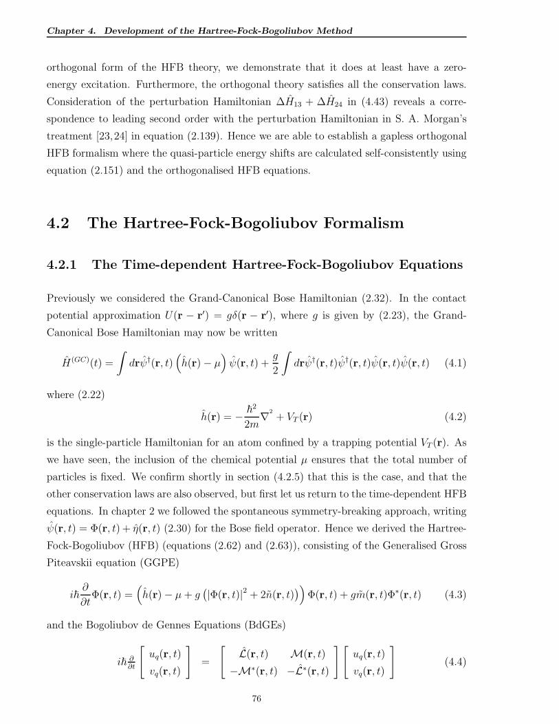
Chapter 4. Development of the Hartree-Fock-Bogoliubov Method
orthogonal form of the HFB theory, we demonstrate that it does at least have a zero-
energy excitation. Furthermore, the orthogonal theory satisfies all the conservation laws.
Consideration of the perturbation Hamiltonian ∆H13 + ∆H24 in (4.43) reveals a corre-
spondence to leading second order with the perturbation Hamiltonian in S. A. Morgan’s
treatment [23,24] in equation (2.139). Hence we are able to establish a gapless orthogonal
HFB formalism where the quasi-particle energy shifts are calculated self-consistently using
equation (2.151) and the orthogonalised HFB equations.
4.2 The Hartree-Fock-Bogoliubov Formalism
4.2.1 The Time-dependent Hartree-Fock-Bogoliubov Equations
Previously we considered the Grand-Canonical Bose Hamiltonian (2.32). In the contact
potential approximation U(r − r′) = gδ(r − r′), where g is given by (2.23), the Grand-
Canonical Bose Hamiltonian may now be written
H(GC)(t) =
∫
drψ†(r, t)(
h(r)− µ)
ψ(r, t) +g
2
∫
drψ†(r, t)ψ†(r, t)ψ(r, t)ψ(r, t) (4.1)
where (2.22)
h(r) = − ~2
2m∇2
+ VT (r) (4.2)
is the single-particle Hamiltonian for an atom confined by a trapping potential VT (r). As
we have seen, the inclusion of the chemical potential µ ensures that the total number of
particles is fixed. We confirm shortly in section (4.2.5) that this is the case, and that the
other conservation laws are also observed, but first let us return to the time-dependent HFB
equations. In chapter 2 we followed the spontaneous symmetry-breaking approach, writing
ψ(r, t) = Φ(r, t) + η(r, t) (2.30) for the Bose field operator. Hence we derived the Hartree-
Fock-Bogoliubov (HFB) (equations (2.62) and (2.63)), consisting of the Generalised Gross
Piteavskii equation (GGPE)
i~∂
∂tΦ(r, t) =
(
h(r)− µ+ g(
|Φ(r, t)|2 + 2n(r, t))
)
Φ(r, t) + gm(r, t)Φ∗(r, t) (4.3)
and the Bogoliubov de Gennes Equations (BdGEs)
i~ ∂∂t
[
uq(r, t)
vq(r, t)
]
=
[
L(r, t) M(r, t)
−M∗(r, t) −L∗(r, t)
][
uq(r, t)
vq(r, t)
]
(4.4)
76
Chapter 4. Development of the Hartree-Fock-Bogoliubov Method
where we defined
L(r, t) ≡ h(r)− µ+ 2g(
|Φ(r, t)|2 + n(r, t))
M(r, t) ≡ g (Φ2(r, t) + m(r, t))(4.5)
with the thermal (2.59), and anomalous (2.60) densities given respectively by
n(r, t) ≡⟨
η†(r, t)η(r, t)⟩
=∑
q
[
|uq(r, t)|2NBE(ǫq) + |vq(r, t)|2 (NBE(ǫq) + 1)]
(4.6)
and
m(r, t) ≡ 〈η(r, t)η(r, t)〉 =∑
q
uq(r, t)v∗q(r, t) (2NBE(ǫq) + 1) (4.7)
where NBE(ǫq) is the Bose distribution for the qth quasi-particle excitation given by (2.51)
NBE(ǫq) =1
exp(βǫq)− 1. (4.8)
The condensate wavefunction Φ(r, t) normalises according to
∫
dr |Φ(r, t)|2 = N − N (4.9)
where N is the total number of atoms, and N the total number of thermal atoms, and the
quasi-particle amplitudes uq(r, t) and vq(r, t) according to (2.54), viz.
∫
dr(
|uq(r, t)|2 − |vq(r, t)|2)
= 1. (4.10)
The total number of thermal atoms N is obtained by integrating the thermal density n(r, t)
over all space, thus
N =
∫
drn(r, t) (4.11)
In the frame rotating with angular frequency Ω the single-particle Bose Hamiltonian is
given by (2.25)
hΩ(r) = − ~2
2m∇2
+ i~Ω · (r×∇) + VT (r). (4.12)
Likewise we can write the expression (2.26)
hv(r) = − ~2
2m∇2
+ i~v · ∇+ VT (r) (4.13)
for the single-particle Bose Hamiltonian in the frame moving with translational velocity v.
77
Chapter 4. Development of the Hartree-Fock-Bogoliubov Method
4.2.2 The Continuity Equation for the Condensate Density
In the Rotating Frame We find from the GGPE (4.3) for the rotating frame
i~∂
∂tΦ(r, t) =
(
hΩ(r)− µ+ g(
|Φ(r, t)|2 + 2n(r, t))
)
Φ(r, t) + gm(r, t)Φ∗(r, t)
and its complex conjugate, the continuity equation for the condensate density
i~∂
∂t|Φ(r, t)|2 =
~2
2m
(
Φ(r, t)∇2Φ∗(r, t)− Φ∗(r, t)∇2Φ(r, t))
+i~Ω·(r×∇) |Φ(r, t)|2+C(r, t)
(4.14)
where we have defined the quantity
C(r, t) ≡ g(
m(r, t)Φ∗2
(r, t)− m∗(r, t)Φ2(r, t))
(4.15)
related to the rate of change of the density of transfer of particles between the condensate
and the thermal population. Defining the current density
j(r, t) ≡ i~
2m(Φ(r, t)∇Φ∗(r, t)− Φ∗(r, t)∇Φ(r, t)) (4.16)
yields the more usual form of the continuity equation for the condensate density
∂
∂t|Φ(r, t)|2 +∇.j(r, t) = Ω · (r×∇) |Φ(r, t)|2 − i
~C(r, t). (4.17)
In the Translating Frame For the translating frame, we obtain the continuity equation
for the condensate density
i~∂
∂t|Φ(r, t)|2 =
~2
2m
(
Φ(r, t)∇2Φ∗(r, t)− Φ∗(r, t)∇2Φ(r, t))
+ i~v · ∇ |Φ(r, t)|2 + C(r, t).
(4.18)
In what follows, we shall make use of the time-independent version of equation (4.14) to
calculate the precessional frequencies of vortices, and of equation (4.18) to calculate the
translational velocity of topological defects in one dimension.
4.2.3 The time-independent HFB Equations
Stationary solutions for the GGPE and the BdGEs are found by substituting the form
Φ(r, t) = Φ(r) exp (−i∆µt/~) (4.19)
78
Chapter 4. Development of the Hartree-Fock-Bogoliubov Method
for the condensate wave function into the time-dependent GGPE (4.3), and the forms
uq(r, t) = uq(r) exp (−iǫqt/~)
vq(r, t) = vq(r) exp (−iǫqt/~)(4.20)
for the quasi-particle amplitudes into the time-dependent BdGEs (4.4), thereby obtaining
the time-independent Generalised Gross Piteavskii equation (GGPE)
(∆µ+ µ)Φ(r) =(
h(r) + g(
|Φ(r)|2 + 2n(r))
)
Φ(r) + gm(r)Φ∗(r) (4.21)
and the time-independent Bogoliubov de Gennes Equations (BdGEs)
ǫq
[
uq(r)
vq(r)
]
=
[
L(r) M(r)
−M∗(r) −L∗(r)
][
uq(r)
vq(r)
]
(4.22)
withL(r) ≡ h(r)− µ+ 2g
(
|Φ(r)|2 + n(r))
M(r) ≡ g (Φ2(r) + m(r)) .(4.23)
(µ + ∆µ) and ǫq are the respective eigenvalues corresponding to the GGPE and BdGEs,
where ∆µ is the difference between the eigenvalue (µ+∆µ) and the true chemical potential
µ. ∆µ and ǫq thus represent the condensate and quasi-particle energies relative to the
system chemical potential µ. The populations of the quasi-particle states are given by
the Bose distribution (4.8), and the ground state population is given likewise by the Bose
distribution (A.30)
Nc = NBE(∆µ) =1
exp(β∆µ)− 1(4.24)
We find that [23, 24]∆µ
kT= ln
(
1 +1
Nc
)
≈ 1
Nc(4.25)
for macroscopic occupation of the ground state (large condensate number Nc). So for
kT ∼ µ, ie. our energy scale is of the order of the chemical potential, which holds for low
temperature T
∆µ ∼ µ
Nc, (4.26)
and we can neglect ∆µ in the low temperature regime. We note that ∆µ→ 0 as Nc →∞,
ie. ∆µ is zero in the thermodynamic limit. Thus the fugacity term
Z = exp
(
∆µ
kBT
)
(4.27)
is very close to unity for low temperature T , so we can ignore it when calculating the
occupation numbers for the quasi-particle modes. The fugacity term referred to here is
used in the calculation of the quasi-particle occupation numbers given by
nq = NBE(ǫq) =1
Z−1 exp(βǫq)− 1. (4.28)
79
Chapter 4. Development of the Hartree-Fock-Bogoliubov Method
and is due to the difference ∆µ between the eigenvalue (µ + ∆µ) and the true chemical
potential µ. The usual definition for the fugacity in statistical mechanics is given by
Z = exp
(
µ
kBT
)
(4.29)
but here the the quasi-particle energies ǫq are already measured relative to the chemical
potential µ. Neglecting ∆µ, we obtain the time-independent GGPE
µΦ(r) =(
h(r) + g(
|Φ(r)|2 + 2n(r))
)
Φ(r) + gm(r)Φ∗(r). (4.30)
4.2.4 The HFB Hamiltonian
We obtain a quadratic approximation for the full Grand-Canonical Hamiltonian (4.1). This
enables us to find an approximate diagonalisation of the Grand-Canonical Hamiltonian, and
hence stationary solutions of the HFB equations. The eigenvalue of the GGPE would then
represent the chemical potential of the system, and the energy eigenvalues of the BdGEs
approximations of the collective excitations for the condensate. We see from linear response
theory that the Bogoliubov approximation gives the collective excitations at T = 0 (see
chapter 2). However for the full HFB, inconsistent treatment for the condensate and non-
condensate due to the symmetry-breaking and the self-consistent mean-field approximation
[11] leads to an unphysical gap in the quasi-particle energy spectrum. Later we shall see how
this energy gap can be removed to reasonable approximation using perturbation theory.
Using the Bogoliubov decomposition ψ(r, t) = Φ(r, t) + η(r, t) and substituting into the
Grand-Canonical Hamiltonian (4.1) and applying the mean field approximations (2.55)
written in terms of the thermal and anomalous densities n(r, t) ≡⟨
η†(r, t)η(r, t)⟩
and
m(r, t) ≡ 〈η(r, t)η(r, t)〉 respectively, and the complex conjugate of the anomalous density
m∗(r, t) ≡⟨
η†(r, t)η†(r, t)⟩
, we were able to approximate the Grand-Canonical Hamiltonian
H(GC)(t) by
H(GC)(t) ≈ HHFB(t) (4.31)
where we defined the HFB hamiltonian given by equations (2.57) and (2.58), breaking
the HFB Hamiltonian into Hamiltonians of zeroth, first and second order in terms of the
annihilation and creation fluctuation operators η and η†, viz. (2.58). We now show that the
time-independent HFB equations diagonalise the HFB Hamiltonian defined by equations
(2.57) and (2.58):
Since∫
drΦ∗hη =∫
dr(
h∗Φ∗)
η and∫
drη†hη =∫
dr(
h∗η†)
η (see appendix B.1.2), we
80
Chapter 4. Development of the Hartree-Fock-Bogoliubov Method
can rewrite HHFB1 and HHFB2 in the form
HHFB1(t) ≡∫
dr(
η†[(
h− µ+ g(
|Φ|2 + 2n)
)
Φ + gmΦ∗]
+ h.c.)
, (4.32)
HHFB2(t) ≡∫
dr
(
1
2η†[(
h− µ+ 2g(
|Φ|2 + n)
)
η + g(
Φ2 + m)
η†]
+ h.c.
)
. (4.33)
Then, substituting the Bogoliubov transformation (2.43) and the time-independent BdGEs
(4.22) for the quasi-particle amplitudes into (4.32) and (4.33), we obtain from the or-
thogonality and symmetry relations (2.53) for the quasi-particle amplitudes, the following
expression for the HFB Hamiltonian (see appendix A.1.3)
HHFB =
∫
dr
(
Φ∗(
h− µ+g
2|Φ|2
)
Φ− g(
n2(r) +1
2|m(r)|2
))
+∑
k
ǫk
(
nk −∫
dr |vk|2)
(4.34)
showing that the time-independent HFB equations (4.30) and (4.22) diagonalise the HFB
Hamiltonian.
4.2.5 Conservation Laws
In any physical theory, it is essential that physical quantities such as total particle number,
energy, angular and linear momentum, etc. are conserved. Here we demonstrate that this
is the case for standard HFB, but that particle and both angular and linear momentum
conservation are violated for Popov, and for the G1 and G2 gapless theories, rendering
them unsuitable for time-dependent simulations.
Particle Conservation
In the Rotating Frame From the continuity equation for the condensate density (4.14)
and the BdGEs (4.4) in the rotating frame, we find that the rate of change in the condensate
and thermal populations are given respectively by (see appendix B.2.1)
dNc(t)
dt= i
g
~
∫
dr(
m(r, t)Φ∗2
(r, t)− m∗(r, t)Φ2(r, t))
(4.35)
anddN(t)
dt= i
g
~
∫
dr(
m∗(r, t)Φ2(r, t)− m(r, t)Φ∗2
(r, t))
(4.36)
where the total number of condensate particles and the total number of thermal (non-
condensate particles are given by Nc(t) =∫
dr |Φ(r, t)|2 and N(t) =∫
drn(r, t) respectively.
81
Chapter 4. Development of the Hartree-Fock-Bogoliubov Method
Therefore the rate of change of condensate particles is the negative of the rate of change
of thermal particles, showing that particles are conserved for time-dependent HFB in the
rotating frame, i.e.d
dt
(
Nc(t) + N(t))
= 0 (4.37)
In the Translating Frame Particle conservation can also be proved in the case of the
translating frame, where the rate of change for the condensate and thermal populations
are given respectively by equations (4.35) and (4.36), and therefore the conservation of
particles (4.37) holds.
It is evident from the above discussion that particles are conserved in general for HFB1.
Violation of Particle Conservation for Popov, and for G1 and G2 Gapless The-
ories To show that particle conservation is violated for the Popov approximation, and
for the gapless G1 and G2 theories, let us write the time-dependent GGPE and BdGEs for
Popov, G1 and G2 as we did in equations (2.74)-(2.80). We obtain (see appendix B.2.1)
dNc
dt= ia
g
~
∫
dr(
mΦ∗2 − m∗Φ2)
+ 2ig
~b
∫
drn
(
mΦ∗
Φ− m∗ Φ
Φ∗
)
(4.38)
and
dN
dt= i
g
~
∫
dr(
m∗Φ2 − mΦ∗2)
+2iag
~
∫
drn
(
m∗ Φ
Φ∗ − mΦ∗
Φ
)
+2ibg
~
∫
drn2
(
m∗
Φ∗2 −m
Φ2
)
(4.39)
Hence we find for Popov (a = b = 0), for G1 (a = 1, b = 0) and for G2 (a = 1, b = 1) that
(see appendix B.2.1)dNc
dt6= −dN
dt(4.40)
so particle conservation is violated in all three cases. As a consequence of this, Popov, and
the G1 and G2 gapless theories are unsuitable candidates for time-dependent simulations.
To explain this we note the scattering processes taken into account in mean-field theory as
shown in figure 4.1. The terms responsible for the transfer of particles between the conden-
sate and the non-condensate are ΦΦη†η† which scatters particles from the condensate into
the non-condensate, and Φ†Φ†ηη which scatters particles from the thermal population into
the condensate. The respective ensemble-averaged terms are Φ2m∗and Φ∗2m, thus we see
1One could also explain this by the fact that HFB is a phi-derivable, and hence a conserving theory
[11, 89]. Therefore one would expect all physical conservation laws to be satisfied, including particle
conservation.
82
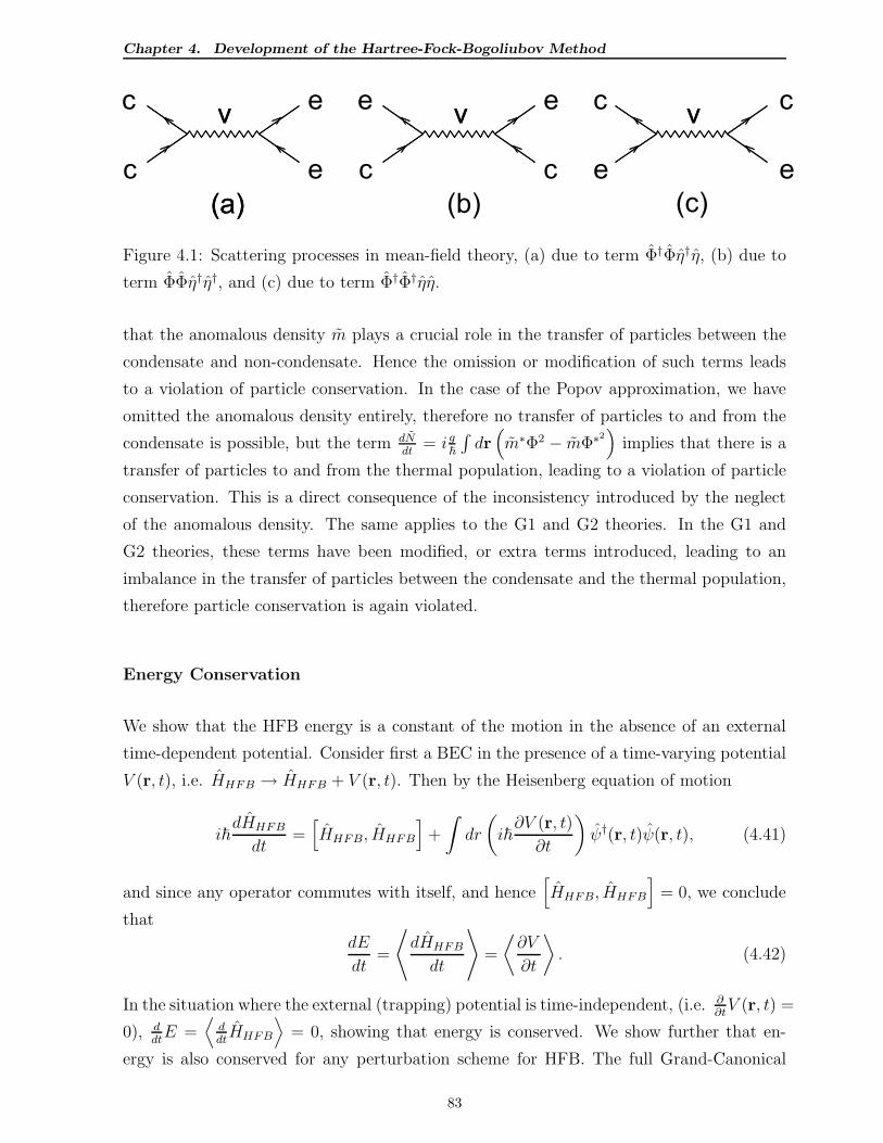
Chapter 4. Development of the Hartree-Fock-Bogoliubov Method
(a)
v
(a)
v vv vv
(b) (c)
c
c
e
e
e e
c c
c c
e e
Figure 4.1: Scattering processes in mean-field theory, (a) due to term Φ†Φη†η, (b) due to
term ΦΦη†η†, and (c) due to term Φ†Φ†ηη.
that the anomalous density m plays a crucial role in the transfer of particles between the
condensate and non-condensate. Hence the omission or modification of such terms leads
to a violation of particle conservation. In the case of the Popov approximation, we have
omitted the anomalous density entirely, therefore no transfer of particles to and from the
condensate is possible, but the term dNdt
= i g~
∫
dr(
m∗Φ2 − mΦ∗2)
implies that there is a
transfer of particles to and from the thermal population, leading to a violation of particle
conservation. This is a direct consequence of the inconsistency introduced by the neglect
of the anomalous density. The same applies to the G1 and G2 theories. In the G1 and
G2 theories, these terms have been modified, or extra terms introduced, leading to an
imbalance in the transfer of particles between the condensate and the thermal population,
therefore particle conservation is again violated.
Energy Conservation
We show that the HFB energy is a constant of the motion in the absence of an external
time-dependent potential. Consider first a BEC in the presence of a time-varying potential
V (r, t), i.e. HHFB → HHFB + V (r, t). Then by the Heisenberg equation of motion
i~dHHFB
dt=[
HHFB, HHFB
]
+
∫
dr
(
i~∂V (r, t)
∂t
)
ψ†(r, t)ψ(r, t), (4.41)
and since any operator commutes with itself, and hence[
HHFB, HHFB
]
= 0, we conclude
that
dE
dt=
⟨
dHHFB
dt
⟩
=
⟨
∂V
∂t
⟩
. (4.42)
In the situation where the external (trapping) potential is time-independent, (i.e. ∂∂tV (r, t) =
0), ddtE =
⟨
ddtHHFB
⟩
= 0, showing that energy is conserved. We show further that en-
ergy is also conserved for any perturbation scheme for HFB. The full Grand-Canonical
83
Chapter 4. Development of the Hartree-Fock-Bogoliubov Method
Hamiltonian of equation (2.34) may be written
H(GC)(t) ≡ HHFB(t) + ∆H13(t) + ∆H24(t) (4.43)
where HHFB(t) is the HFB Hamiltonian given by (2.57)
HHFB(t) ≡ HHFB0(t) + HHFB1(t) + HHFB2(t) (4.44)
where we have broken the HFB Hamiltonian into Hamiltonians of zeroth, first and second
order in terms of the annihilation and creation fluctuation operators η and η† with HHFB0(t)
given by the first of equations (2.58), and HHFB1(t) and HHFB2(t) respectively by equations
(4.32) and (4.33) . In view of the approximate decomposition (2.55), the residual of the
full Grand-Canonical Hamiltonian may be written ∆H(t) ≡ ∆H13(t) + ∆H24(t) where
∆H13(t) = ∆H1(t) + ∆H3(t),
∆H24(t) = ∆H2(t) + ∆H4(t)(4.45)
where the first, second, third and fourth order perturbation Hamiltonians in the thermal
fluctuation operator η are given by
∆H1(t) = −g∫
dr(
(2Φ∗n + Φm∗) η + (2Φn + Φ∗m) η†)
,
∆H2(t) = −g2
∫
dr(
4nη†η + m∗ηη + mη†η†)
,
∆H3(t) = g∫
dr(
Φ∗η†ηη + Φη†η†η)
, and
∆H4(t) = g2
∫
drη†η†ηη,
(4.46)
where we note that ∆H3(t) ≡ H(GC)3 , ∆H4(t) ≡ H
(GC)4 . It can be shown that (see appendix
B.2.2)⟨[
HHFB(t),∆H13(t)]⟩
=⟨[
HHFB(t),∆H24(t)]⟩
= 0 (4.47)
Hence for a time-independent external trapping potential,
⟨
i~dHHFB(t)
dt
⟩
=⟨[
HHFB(t), H(t)]⟩
=⟨[
HHFB(t),∆H13(t)]⟩
+⟨[
HHFB(t),∆H24(t)]⟩
= 0
(4.48)
showing that energy is still conserved.
An alternative proof of the conservation of energy for HFB is shown at the end of appendix
B.2.2, and reveals that energy conservation is violated in the cases of the Popov, G1 and
G2 approximations.
84
Chapter 4. Development of the Hartree-Fock-Bogoliubov Method
Conservation of Angular Momentum
One would expect the angular momentum of the BEC system to be conserved in the absence
of any external potential, but that the introduction of an external potential may or may
not affect the angular momentum of the system, depending on the symmetry properties of
the external potential. We anticipate that the quantum expectation value of the angular
momentum operator L defined by L ≡ i~ (r×∇) of the BEC be conserved in a spherically
symmetric harmonic trap, and this will become evident shortly.
The quantum expectation value of the angular momentum is given by
⟨
L⟩
=
⟨∫
drψ†(r, t)Lψ(r, t)
⟩
, (4.49)
and the rate of change of⟨
L⟩
, the ensemble-averaged angular momentum of the BEC is
given by
d⟨
L⟩
dt=
d
dt
⟨∫
drψ†(r, t)Lψ(r, t)
⟩
(4.50)
Since ψ(r, t) = Φ(r, t) + η(r, t) by (2.30), we find that
d⟨
L⟩
dt=
1
i~
⟨∫
dr
[
i~∂
∂tΦ∗LΦ + Φ∗L
(
i~∂
∂tΦ
)
+ i~∂η†
∂tLη + η†L
(
i~∂η
∂t
)]⟩
. (4.51)
Substituting the time-dependent GGPE (4.3) and the time-dependent BdGEs (4.4) and
their respective complex conjugates into (4.51) and applying the results in appendix B.1.2
for Bose field operators, we obtain (see appendix B.2.3)
d⟨
L⟩
dt=
1
i~
∫
dr(
|Φ|2 + n)
LVT . (4.52)
The conservation of angular momentum therefore depends entirely on the trapping poten-
tial and/or any other externally applied potential, as one would expect. Angular momen-
tum is conserved whenever LVT = 0. This is clearly the case whenever spherical symmetry
exists, thus angular momentum is conserved in a spherically symmetric harmonic trap, i.e.
d⟨
L⟩
dt= 0. (4.53)
In an axially symmetric harmonic trap, LzVT = 0, so the ensemble-averaged z-component
(i.e. the component along the axis of symmetry) of angular momentum is conserved, i.e.
d⟨
Lz
⟩
dt= 0. (4.54)
85
Chapter 4. Development of the Hartree-Fock-Bogoliubov Method
Clearly the angular momentum is always conserved in the absence of any trapping potential
(VT = 0).
This holds for any linear differential operator D, i.e. ddtD =
∫
dr(
|Φ|2 + n)
DVT , therefore
the same result applies to linear momentum.
Violation of angular momentum conservation for Popov, G1 and G2
We show that conservation of the expectation value of the angular momentum L of the
BEC is violated for Popov, G1 and G2, whether a trapping potential is present or not.
From appendix B.2.3, we obtain the expression
d⟨
L⟩
dt=
∫
dr[
(
|Φ|2 + n)
LVT
]
+ IR (4.55)
where
IR =2g
~Re
1
i
∫
dr
[
−(a− 1)m∗ΦL (Φ)− 2bm∗ nΦ
|Φ|2L (Φ)− 2m∗
(
a |Φ|2 + bn)
Φ∗2
⟨
η†Lη⟩
]
.
(4.56)
For Popov a = b = 0, for G1 a = 1, b = 0, and for G2 a = b = 1, IR is given respectively
by equations (B.68), (B.69) and (B.70) for Popov, G1 and G2. In general, IR 6= 0, so
angular momentum conservation is violated in all three cases, regardless of the trapping
potential, and this is illustrated in Appendix F, section F.1 in a time-dependent simulation
(repeating the third time-dependent simulation carried out in section 7.5.2 of chapter 7)
deploying the G1 approximation. In this simulation, the violation of number and angular
momentum are clearly illustrated.
We see from the previous section that all physical conservation laws are observed for the full
HFB formalism. This is not surprising since HFB is phi-derivable and hence a conserving
theory [11, 89].
4.2.6 Calculation of the Angular Momentum in the Rotating
Frame
The quantum expectation value of the angular momentum L is given by
⟨
L⟩
=
⟨∫
drψ†(r, t)Lψ(r, t)
⟩
=
∫
dr[
Φ∗(r, t)LΦ(r, t) +⟨
η†(r, t)L (η(r, t))⟩]
(4.57)
86
Chapter 4. Development of the Hartree-Fock-Bogoliubov Method
From the Bogoliubov transformation (2.43), and its Hermitian conjugate (2.44), and apply-
ing Wick’s theorem for ensemble averages of operator pairs a†kal, we obtain the expression
⟨
L⟩
= i~
∫
dr
[
Φ∗ (r×∇) Φ +∑
q
(
nqu∗q (r×∇) uq + (nq + 1) vq (r×∇) v∗q
)
]
(4.58)
for L.
4.2.7 Calculation of the Precessional Frequency of Off-axis Vor-
tices in Quasi-2D BECs
The precessional frequency of vortices may be predicted by using the time-independent
HFB equations and the time-independent continuity equation for the condensate density to
find the stationary solution for an off-axis vortex in the frame rotating at the precessional
frequency of the vortex. The time-independent continuity equation for the condensate
density is used to derive a suitable expression for the precessional frequency of off-axis
vortices. We consider a stationary vortex system in the frame rotating at the precessional
frequency of the off-axis vortex or vortices. This is solved self-consistently with the HFB
equations in this rotating frame.
We derive a suitable expression for the rotational frequency from the time independent
continuity equation for the condensate density (4.14) by writing the condensate wave-
function Φ(r, t) in terms of its real and imaginary parts R(r, t) and I(r, t),
Φ(r, t) = R(r, t) + iI(r, t), (4.59)
hence we find for a stationary solution (∂/∂t |Φ(r, t)|2 ≡ 0)
~Ω · (r×∇) |Φ(r)|2 = 2~
2
2m
(
R(r)∇2I(r)− I(r)∇2R(r))
+ iC(r) (4.60)
where we have defined the quantity
C(r) ≡ g(
m(r)Φ∗2
(r)− m∗(r)Φ2(r))
.
It is convenient to represent the 2D system in polar coordinates (as we will be making use
of the Laguerre polynomials for the basis functions). Writing R ≡ R(r, θ), I ≡ I(r, θ), we
find that
Ωr2A(r, θ) = B(r, θ) (4.61)
where we have defined
A(r, θ) ≡(
R∂R
∂θ+ I
∂I
∂θ
)
(4.62)
87
Chapter 4. Development of the Hartree-Fock-Bogoliubov Method
and
B(r, θ) ≡ ~
2m
[
r2
(
R∂2I
∂r2− I ∂
2R
∂r2
)
+ r
(
R∂I
∂r− I ∂R
∂r
)
+
(
R∂2I
∂θ2− I ∂
2R
∂θ2
)]
+ ir2
2~C(r, θ)
(4.63)
with
C(r, θ) ≡ g(
mΦ∗2 − m∗Φ2)
. (4.64)
Multiplying both sides by A(r, θ), and integrating over all space gives us the expression
Ω =
∫ 2π
0
∫∞0A(r, θ)B(r, θ)rdrdθ
∫ 2π
0
∫∞0r2 (A(r, θ))2 rdrdθ
. (4.65)
This result is important for two reasons:
1. It allows us to predict the precessional frequency for single off-axis vortices and
for vortex arrays, allowing us to place the vortices in any desired position. For a
single vortex one could choose a precessional frequency, solve the HFB equations self-
consistently and then see where the vortex lies. However this does not provide us with
a prediction of the precessional frequency of the vortices, and this procedure is not
possible for vortex arrays. This provides us with a useful method for generating any
desired vortex array, allowing us then to investigate the effect of symmetry-breaking
of the trapping potential, the introduction of noise into the system by means of an
external perturbing potential (i.e. HHFB → HHFB + V (r, t)) where the externally
applied potential V (r, t) consists of white noise, etc. using the time-dependent HFB
equations to study the behaviour of the system.
2. This result demonstrates that the precession of the vortex is due to conservation of
mass flow described by the continuity equation for the condensate density, and not
by the LCLS energies as was originally asserted in [2, 3] - see chapter 7.
4.2.8 Calculation of the Translational Velocity of Topological De-
fects in 1D BECs in Toroidal Traps
We derive a similar expression for the translational velocity as follows. The time indepen-
dent continuity equation for the condensate density in the translating frame is given by
(4.18) and by writing Φ(r, t) in terms of its real and imaginary parts (4.59) as before. We
find for a stationary solution (∂/∂t |Φ(r, t)|2 ≡ 0)
~v.∇ |Φ(r)|2 = 2~2
2m
(
R(r)∇2I(r)− I(r)∇2R(r))
+ iC(r) (4.66)
88
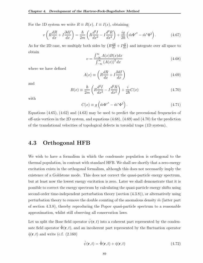
Chapter 4. Development of the Hartree-Fock-Bogoliubov Method
For the 1D system we write R ≡ R(x), I ≡ I(x), obtaining
v
(
RdR
dx+ I
∂dI
dx
)
=~
2m
(
Rd2I
dx2− I d
2R
dx2
)
+ig
2~
(
mΦ∗2 − m∗Φ2)
. (4.67)
As for the 2D case, we multiply both sides by(
RdRdx
+ I dIdx
)
and integrate over all space to
obtain
v =
∫∞−∞A(x)B(x)dx∫∞−∞ (A(x))2 dx
(4.68)
where we have defined
A(x) ≡(
RdR
dx+ I
∂dI
dx
)
(4.69)
and
B(x) ≡ ~
2m
(
Rd2I
dx2− I d
2R
dx2
)
+i
2~C(x) (4.70)
with
C(x) ≡ g(
mΦ∗2 − m∗Φ2)
. (4.71)
Equations (4.65), (4.62) and (4.63) may be used to predict the precessional frequencies of
off-axis vortices in the 2D system, and equations (4.68), (4.69) and (4.70) for the prediction
of the translational velocities of topological defects in toroidal traps (1D system).
4.3 Orthogonal HFB
We wish to have a formalism in which the condensate population is orthogonal to the
thermal population, in contrast with standard HFB. We shall see shortly that a zero-energy
excitation exists in the orthogonal formalism, although this does not necessarily imply the
existence of a Goldstone mode. This does not correct the quasi-particle energy spectrum,
but at least now the lowest energy excitation is zero. Later we shall demonstrate that it is
possible to correct the energy spectrum by calculating the quasi-particle energy shifts using
second-order time-independent perturbation theory (section (4.3.8)), or alternatively using
perturbation theory to remove the double counting of the anomalous density m (latter part
of section 4.3.8), thereby reproducing the Popov quasi-particle spectrum to a reasonable
approximation, whilst still observing all conservation laws.
Let us split the Bose field operator ψ(r, t) into a coherent part represented by the conden-
sate field operator Φ(r, t), and an incoherent part represented by the fluctuation operator
η(r, t) and write (c.f. (2.160)
ψ(r, t) = Φ(r, t) + η(r, t) (4.72)
89
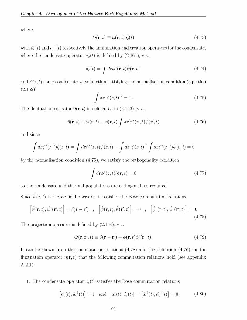
Chapter 4. Development of the Hartree-Fock-Bogoliubov Method
where
Φ(r, t) ≡ φ(r, t)ac(t) (4.73)
with ac(t) and ac†(t) respectively the annihilation and creation operators for the condensate,
where the condensate operator ac(t) is defined by (2.161), viz.
ac(t) =
∫
drφ∗(r, t)ψ(r, t). (4.74)
and φ(r, t) some condensate wavefunction satisfying the normalisation condition (equation
(2.162))∫
dr |φ(r, t)|2 = 1. (4.75)
The fluctuation operator η(r, t) is defined as in (2.163), viz.
η(r, t) ≡ ψ(r, t)− φ(r, t)
∫
dr′φ∗(r′, t)ψ(r′, t) (4.76)
and since∫
drφ∗(r, t)η(r, t) =
∫
drφ∗(r, t)ψ(r, t)−∫
dr |φ(r, t)|2∫
drφ∗(r, t)ψ(r, t) = 0
by the normalisation condition (4.75), we satisfy the orthogonality condition
∫
drφ∗(r, t)η(r, t) = 0 (4.77)
so the condensate and thermal populations are orthogonal, as required.
Since ψ(r, t) is a Bose field operator, it satisfies the Bose commutation relations
[
ψ(r, t), ψ†(r′, t)]
= δ(r− r′) ,[
ψ(r, t), ψ(r′, t)]
= 0 ,[
ψ†(r, t), ψ†(r′, t)]
= 0.
(4.78)
The projection operator is defined by (2.164), viz.
Q(r, r′, t) ≡ δ(r− r′)− φ(r, t)φ∗(r′, t). (4.79)
It can be shown from the commutation relations (4.78) and the definition (4.76) for the
fluctuation operator η(r, t) that the following commutation relations hold (see appendix
A.2.1):
1. The condensate operator ac(t) satisfies the Bose commutation relations
[
ac(t), ac†(t)]
= 1 and [ac(t), ac(t)] =[
ac†(t), ac
†(t)]
= 0, (4.80)
90
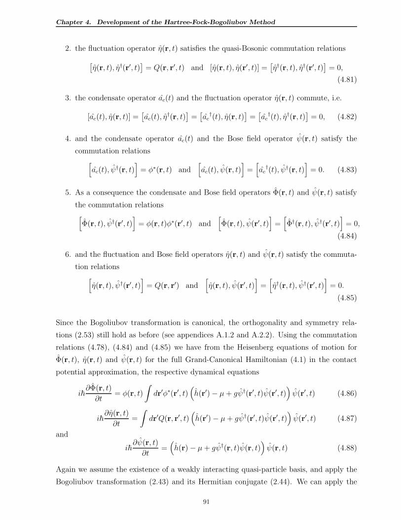
Chapter 4. Development of the Hartree-Fock-Bogoliubov Method
2. the fluctuation operator η(r, t) satisfies the quasi-Bosonic commutation relations
[
η(r, t), η†(r′, t)]
= Q(r, r′, t) and [η(r, t), η(r′, t)] =[
η†(r, t), η†(r′, t)]
= 0,
(4.81)
3. the condensate operator ac(t) and the fluctuation operator η(r, t) commute, i.e.
[ac(t), η(r, t)] =[
ac(t), η†(r, t)
]
=[
ac†(t), η(r, t)
]
=[
ac†(t), η†(r, t)
]
= 0, (4.82)
4. and the condensate operator ac(t) and the Bose field operator ψ(r, t) satisfy the
commutation relations
[
ac(t), ψ†(r, t)
]
= φ∗(r, t) and[
ac(t), ψ(r, t)]
=[
ac†(t), ψ†(r, t)
]
= 0. (4.83)
5. As a consequence the condensate and Bose field operators Φ(r, t) and ψ(r, t) satisfy
the commutation relations
[
Φ(r, t), ψ†(r′, t)]
= φ(r, t)φ∗(r′, t) and[
Φ(r, t), ψ(r′, t)]
=[
Φ†(r, t), ψ†(r′, t)]
= 0,
(4.84)
6. and the fluctuation and Bose field operators η(r, t) and ψ(r, t) satisfy the commuta-
tion relations
[
η(r, t), ψ†(r′, t)]
= Q(r, r′) and[
η(r, t), ψ(r′, t)]
=[
η†(r, t), ψ†(r′, t)]
= 0.
(4.85)
Since the Bogoliubov transformation is canonical, the orthogonality and symmetry rela-
tions (2.53) still hold as before (see appendices A.1.2 and A.2.2). Using the commutation
relations (4.78), (4.84) and (4.85) we have from the Heisenberg equations of motion for
Φ(r, t), η(r, t) and ψ(r, t) for the full Grand-Canonical Hamiltonian (4.1) in the contact
potential approximation, the respective dynamical equations
i~∂Φ(r, t)
∂t= φ(r, t)
∫
dr′φ∗(r′, t)(
h(r′)− µ+ gψ†(r′, t)ψ(r′, t))
ψ(r′, t) (4.86)
i~∂η(r, t)
∂t=
∫
dr′Q(r, r′, t)(
h(r′)− µ+ gψ†(r′, t)ψ(r′, t))
ψ(r′, t) (4.87)
and
i~∂ψ(r, t)
∂t=(
h(r)− µ+ gψ†(r, t)ψ(r, t))
ψ(r, t) (4.88)
Again we assume the existence of a weakly interacting quasi-particle basis, and apply the
Bogoliubov transformation (2.43) and its Hermitian conjugate (2.44). We can apply the
91
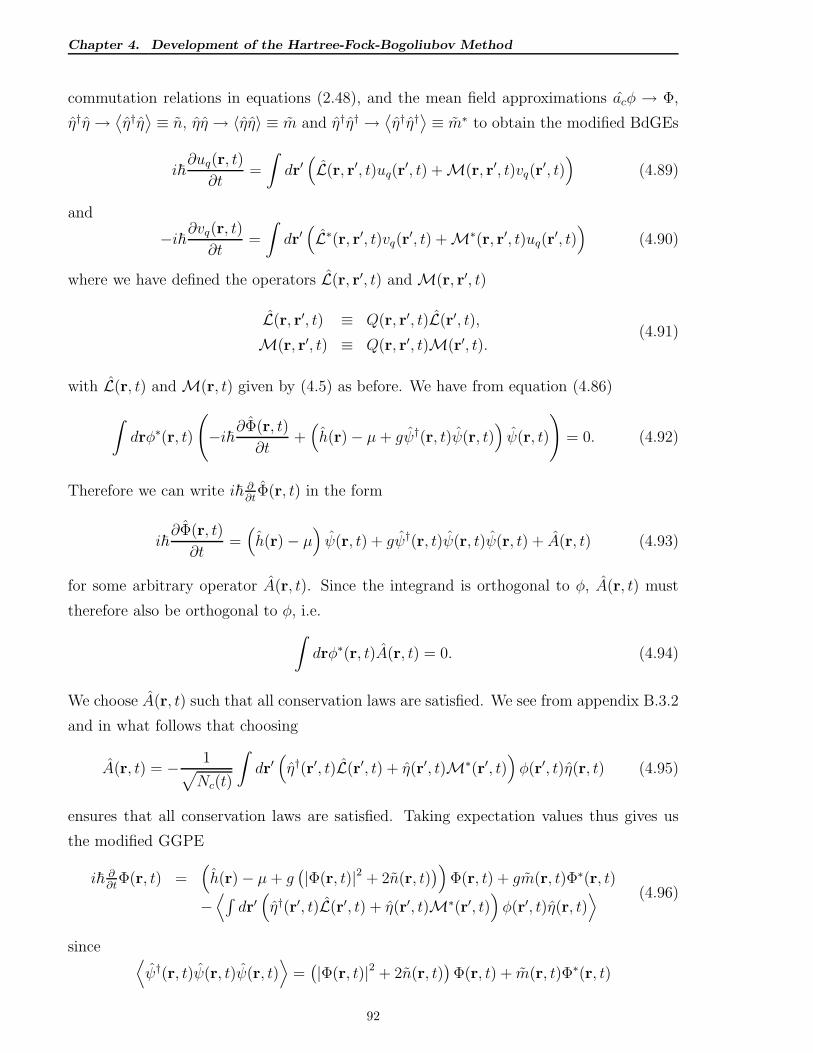
Chapter 4. Development of the Hartree-Fock-Bogoliubov Method
commutation relations in equations (2.48), and the mean field approximations acφ → Φ,
η†η →⟨
η†η⟩
≡ n, ηη → 〈ηη〉 ≡ m and η†η† →⟨
η†η†⟩
≡ m∗ to obtain the modified BdGEs
i~∂uq(r, t)
∂t=
∫
dr′(
L(r, r′, t)uq(r′, t) +M(r, r′, t)vq(r
′, t))
(4.89)
and
−i~∂vq(r, t)
∂t=
∫
dr′(
L∗(r, r′, t)vq(r′, t) +M∗(r, r′, t)uq(r
′, t))
(4.90)
where we have defined the operators L(r, r′, t) andM(r, r′, t)
L(r, r′, t) ≡ Q(r, r′, t)L(r′, t),
M(r, r′, t) ≡ Q(r, r′, t)M(r′, t).(4.91)
with L(r, t) andM(r, t) given by (4.5) as before. We have from equation (4.86)
∫
drφ∗(r, t)
(
−i~∂Φ(r, t)
∂t+(
h(r)− µ+ gψ†(r, t)ψ(r, t))
ψ(r, t)
)
= 0. (4.92)
Therefore we can write i~ ∂∂t
Φ(r, t) in the form
i~∂Φ(r, t)
∂t=(
h(r)− µ)
ψ(r, t) + gψ†(r, t)ψ(r, t)ψ(r, t) + A(r, t) (4.93)
for some arbitrary operator A(r, t). Since the integrand is orthogonal to φ, A(r, t) must
therefore also be orthogonal to φ, i.e.
∫
drφ∗(r, t)A(r, t) = 0. (4.94)
We choose A(r, t) such that all conservation laws are satisfied. We see from appendix B.3.2
and in what follows that choosing
A(r, t) = − 1√
Nc(t)
∫
dr′(
η†(r′, t)L(r′, t) + η(r′, t)M∗(r′, t))
φ(r′, t)η(r, t) (4.95)
ensures that all conservation laws are satisfied. Taking expectation values thus gives us
the modified GGPE
i~ ∂∂t
Φ(r, t) =(
h(r)− µ+ g(
|Φ(r, t)|2 + 2n(r, t))
)
Φ(r, t) + gm(r, t)Φ∗(r, t)
−⟨
∫
dr′(
η†(r′, t)L(r′, t) + η(r′, t)M∗(r′, t))
φ(r′, t)η(r, t)⟩ (4.96)
since⟨
ψ†(r, t)ψ(r, t)ψ(r, t)⟩
=(
|Φ(r, t)|2 + 2n(r, t))
Φ(r, t) + m(r, t)Φ∗(r, t)
92
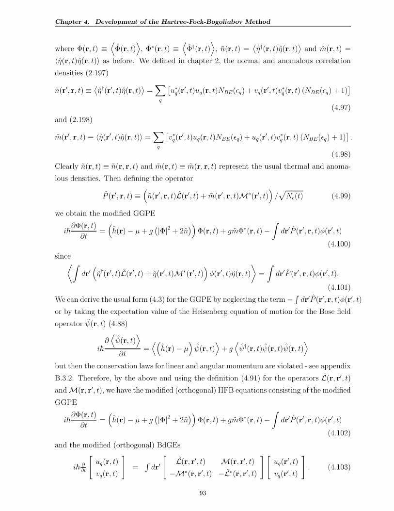
Chapter 4. Development of the Hartree-Fock-Bogoliubov Method
where Φ(r, t) ≡⟨
Φ(r, t)⟩
, Φ∗(r, t) ≡⟨
Φ†(r, t)⟩
, n(r, t) =⟨
η†(r, t)η(r, t)⟩
and m(r, t) =
〈η(r, t)η(r, t)〉 as before. We defined in chapter 2, the normal and anomalous correlation
densities (2.197)
n(r′, r, t) ≡⟨
η†(r′, t)η(r, t)⟩
=∑
q
[
u∗q(r′, t)uq(r, t)NBE(ǫq) + vq(r
′, t)v∗q (r, t) (NBE(ǫq) + 1)]
(4.97)
and (2.198)
m(r′, r, t) ≡ 〈η(r′, t)η(r, t)〉 =∑
q
[
v∗q (r′, t)uq(r, t)NBE(ǫq) + uq(r
′, t)v∗q (r, t) (NBE(ǫq) + 1)]
.
(4.98)
Clearly n(r, t) ≡ n(r, r, t) and m(r, t) ≡ m(r, r, t) represent the usual thermal and anoma-
lous densities. Then defining the operator
P (r′, r, t) ≡(
n(r′, r, t)L(r′, t) + m(r′, r, t)M∗(r′, t))
/√
Nc(t) (4.99)
we obtain the modified GGPE
i~∂Φ(r, t)
∂t=(
h(r)− µ+ g(
|Φ|2 + 2n)
)
Φ(r, t) + gmΦ∗(r, t)−∫
dr′P (r′, r, t)φ(r′, t)
(4.100)
since⟨∫
dr′(
η†(r′, t)L(r′, t) + η(r′, t)M∗(r′, t))
φ(r′, t)η(r, t)
⟩
=
∫
dr′P (r′, r, t)φ(r′, t).
(4.101)
We can derive the usual form (4.3) for the GGPE by neglecting the term−∫
dr′P (r′, r, t)φ(r′, t)
or by taking the expectation value of the Heisenberg equation of motion for the Bose field
operator ψ(r, t) (4.88)
i~∂⟨
ψ(r, t)⟩
∂t=⟨(
h(r)− µ)
ψ(r, t)⟩
+ g⟨
ψ†(r, t)ψ(r, t)ψ(r, t)⟩
but then the conservation laws for linear and angular momentum are violated - see appendix
B.3.2. Therefore, by the above and using the definition (4.91) for the operators L(r, r′, t)
andM(r, r′, t), we have the modified (orthogonal) HFB equations consisting of the modified
GGPE
i~∂Φ(r, t)
∂t=(
h(r)− µ+ g(
|Φ|2 + 2n)
)
Φ(r, t) + gmΦ∗(r, t)−∫
dr′P (r′, r, t)φ(r′, t)
(4.102)
and the modified (orthogonal) BdGEs
i~ ∂∂t
[
uq(r, t)
vq(r, t)
]
=∫
dr′
[
L(r, r′, t) M(r, r′, t)
−M∗(r, r′, t) −L∗(r, r′, t)
][
uq(r′, t)
vq(r′, t)
]
. (4.103)
93
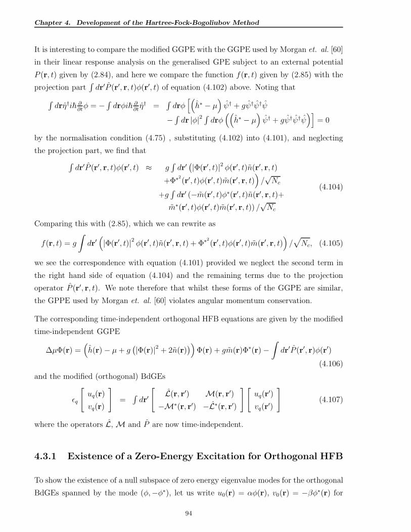
Chapter 4. Development of the Hartree-Fock-Bogoliubov Method
It is interesting to compare the modified GGPE with the GGPE used by Morgan et. al. [60]
in their linear response analysis on the generalised GPE subject to an external potential
P (r, t) given by (2.84), and here we compare the function f(r, t) given by (2.85) with the
projection part∫
dr′P (r′, r, t)φ(r′, t) of equation (4.102) above. Noting that
∫
drη†i~ ∂∂tφ = −
∫
drφi~ ∂∂tη† =
∫
drφ[(
h∗ − µ)
ψ† + gψ†ψ†ψ
−∫
dr |φ|2∫
drφ((
h∗ − µ)
ψ† + gψ†ψ†ψ)]
= 0
by the normalisation condition (4.75) , substituting (4.102) into (4.101), and neglecting
the projection part, we find that
∫
dr′P (r′, r, t)φ(r′, t) ≈ g∫
dr′(
|Φ(r′, t)|2 φ(r′, t)n(r′, r, t)
+Φ∗2(r′, t)φ(r′, t)m(r′, r, t)
)
/√Nc
+g∫
dr′ (−m(r′, t)φ∗(r′, t)n(r′, r, t)+
m∗(r′, t)φ(r′, t)m(r′, r, t)) /√Nc
(4.104)
Comparing this with (2.85), which we can rewrite as
f(r, t) = g
∫
dr′(
|Φ(r′, t)|2 φ(r′, t)n(r′, r, t) + Φ∗2
(r′, t)φ(r′, t)m(r′, r, t))
/√
Nc, (4.105)
we see the correspondence with equation (4.101) provided we neglect the second term in
the right hand side of equation (4.104) and the remaining terms due to the projection
operator P (r′, r, t). We note therefore that whilst these forms of the GGPE are similar,
the GPPE used by Morgan et. al. [60] violates angular momentum conservation.
The corresponding time-independent orthogonal HFB equations are given by the modified
time-independent GGPE
∆µΦ(r) =(
h(r)− µ+ g(
|Φ(r)|2 + 2n(r))
)
Φ(r) + gm(r)Φ∗(r)−∫
dr′P (r′, r)φ(r′)
(4.106)
and the modified (orthogonal) BdGEs
ǫq
[
uq(r)
vq(r)
]
=∫
dr′
[
L(r, r′) M(r, r′)
−M∗(r, r′) −L∗(r, r′)
][
uq(r′)
vq(r′)
]
(4.107)
where the operators L,M and P are now time-independent.
4.3.1 Existence of a Zero-Energy Excitation for Orthogonal HFB
To show the existence of a null subspace of zero energy eigenvalue modes for the orthogonal
BdGEs spanned by the mode (φ,−φ∗), let us write u0(r) = αφ(r), v0(r) = −βφ∗(r) for
94
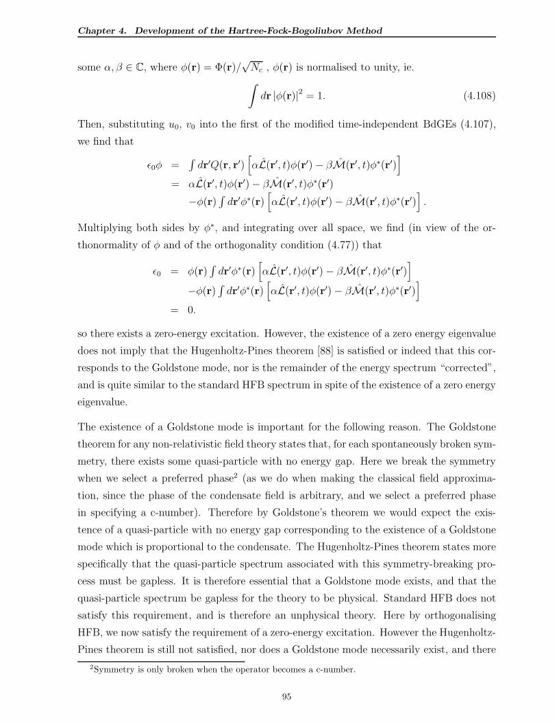
Chapter 4. Development of the Hartree-Fock-Bogoliubov Method
some α, β ∈ C, where φ(r) = Φ(r)/√Nc , φ(r) is normalised to unity, ie.
∫
dr |φ(r)|2 = 1. (4.108)
Then, substituting u0, v0 into the first of the modified time-independent BdGEs (4.107),
we find that
ǫ0φ =∫
dr′Q(r, r′)[
αL(r′, t)φ(r′)− βM(r′, t)φ∗(r′)]
= αL(r′, t)φ(r′)− βM(r′, t)φ∗(r′)
−φ(r)∫
dr′φ∗(r)[
αL(r′, t)φ(r′)− βM(r′, t)φ∗(r′)]
.
Multiplying both sides by φ∗, and integrating over all space, we find (in view of the or-
thonormality of φ and of the orthogonality condition (4.77)) that
ǫ0 = φ(r)∫
dr′φ∗(r)[
αL(r′, t)φ(r′)− βM(r′, t)φ∗(r′)]
−φ(r)∫
dr′φ∗(r)[
αL(r′, t)φ(r′)− βM(r′, t)φ∗(r′)]
= 0.
so there exists a zero-energy excitation. However, the existence of a zero energy eigenvalue
does not imply that the Hugenholtz-Pines theorem [88] is satisfied or indeed that this cor-
responds to the Goldstone mode, nor is the remainder of the energy spectrum “corrected”,
and is quite similar to the standard HFB spectrum in spite of the existence of a zero energy
eigenvalue.
The existence of a Goldstone mode is important for the following reason. The Goldstone
theorem for any non-relativistic field theory states that, for each spontaneously broken sym-
metry, there exists some quasi-particle with no energy gap. Here we break the symmetry
when we select a preferred phase2 (as we do when making the classical field approxima-
tion, since the phase of the condensate field is arbitrary, and we select a preferred phase
in specifying a c-number). Therefore by Goldstone’s theorem we would expect the exis-
tence of a quasi-particle with no energy gap corresponding to the existence of a Goldstone
mode which is proportional to the condensate. The Hugenholtz-Pines theorem states more
specifically that the quasi-particle spectrum associated with this symmetry-breaking pro-
cess must be gapless. It is therefore essential that a Goldstone mode exists, and that the
quasi-particle spectrum be gapless for the theory to be physical. Standard HFB does not
satisfy this requirement, and is therefore an unphysical theory. Here by orthogonalising
HFB, we now satisfy the requirement of a zero-energy excitation. However the Hugenholtz-
Pines theorem is still not satisfied, nor does a Goldstone mode necessarily exist, and there
2Symmetry is only broken when the operator becomes a c-number.
95
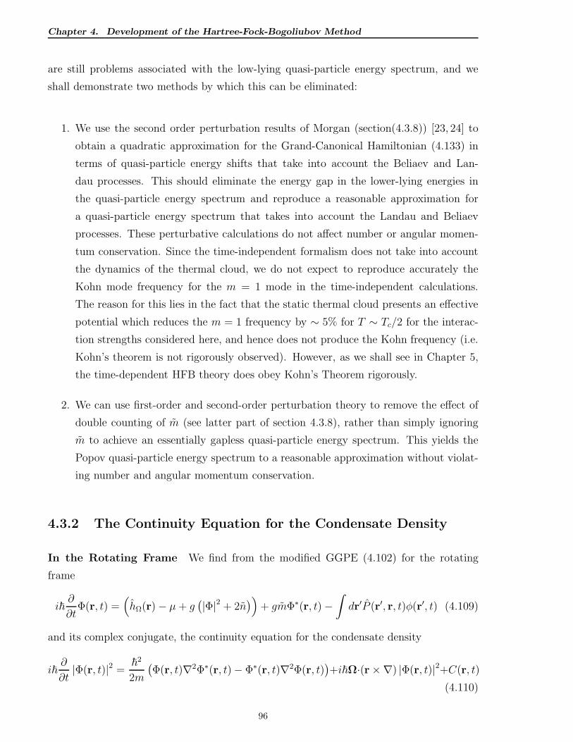
Chapter 4. Development of the Hartree-Fock-Bogoliubov Method
are still problems associated with the low-lying quasi-particle energy spectrum, and we
shall demonstrate two methods by which this can be eliminated:
1. We use the second order perturbation results of Morgan (section(4.3.8)) [23, 24] to
obtain a quadratic approximation for the Grand-Canonical Hamiltonian (4.133) in
terms of quasi-particle energy shifts that take into account the Beliaev and Lan-
dau processes. This should eliminate the energy gap in the lower-lying energies in
the quasi-particle energy spectrum and reproduce a reasonable approximation for
a quasi-particle energy spectrum that takes into account the Landau and Beliaev
processes. These perturbative calculations do not affect number or angular momen-
tum conservation. Since the time-independent formalism does not take into account
the dynamics of the thermal cloud, we do not expect to reproduce accurately the
Kohn mode frequency for the m = 1 mode in the time-independent calculations.
The reason for this lies in the fact that the static thermal cloud presents an effective
potential which reduces the m = 1 frequency by ∼ 5% for T ∼ Tc/2 for the interac-
tion strengths considered here, and hence does not produce the Kohn frequency (i.e.
Kohn’s theorem is not rigorously observed). However, as we shall see in Chapter 5,
the time-dependent HFB theory does obey Kohn’s Theorem rigorously.
2. We can use first-order and second-order perturbation theory to remove the effect of
double counting of m (see latter part of section 4.3.8), rather than simply ignoring
m to achieve an essentially gapless quasi-particle energy spectrum. This yields the
Popov quasi-particle energy spectrum to a reasonable approximation without violat-
ing number and angular momentum conservation.
4.3.2 The Continuity Equation for the Condensate Density
In the Rotating Frame We find from the modified GGPE (4.102) for the rotating
frame
i~∂
∂tΦ(r, t) =
(
hΩ(r)− µ+ g(
|Φ|2 + 2n)
)
+ gmΦ∗(r, t)−∫
dr′P (r′, r, t)φ(r′, t) (4.109)
and its complex conjugate, the continuity equation for the condensate density
i~∂
∂t|Φ(r, t)|2 =
~2
2m
(
Φ(r, t)∇2Φ∗(r, t)− Φ∗(r, t)∇2Φ(r, t))
+i~Ω·(r×∇) |Φ(r, t)|2+C(r, t)
(4.110)
96
Chapter 4. Development of the Hartree-Fock-Bogoliubov Method
where we now define the quantity C(r, t) by
C(r, t) ≡ g(
m(r, t)Φ∗2
(r, t)− m∗(r, t)Φ2(r, t))
+G∗(r, t)−G(r, t) (4.111)
with
G(r, t) ≡ Φ∗(r, t)
∫
dr′P (r′, r, t)φ(r′, t). (4.112)
The corresponding time-independent continuity equation for the condensate density is given
by
~2
2m
(
Φ(r)∇2Φ∗(r)− Φ∗(r)∇2Φ(r))
+ i~Ω · (r×∇) |Φ(r)|2 + C(r) = 0. (4.113)
In the Translating Frame For the translating frame, we obtain the continuity equation
for the condensate density
i~∂
∂t|Φ(r, t)|2 =
~2
2m
(
Φ(r, t)∇2Φ∗(r, t)− Φ∗(r, t)∇2Φ(r, t))
+ i~v · ∇ |Φ(r, t)|2 + C(r, t)
(4.114)
with corresponding time-independent continuity equation for the condensate density
~2
2m
(
Φ(r)∇2Φ∗(r)− Φ∗(r)∇2Φ(r))
+ i~v · ∇ |Φ(r)|2 + C(r) = 0. (4.115)
4.3.3 Particle Conservation for Orthogonal HFB
Having established an orthogonal formalism, it is now important to show that the conser-
vation laws are still observed, as is the case with standard HFB. We begin with particle
conservation.
Since∫
drdr′Φ∗(r, t)P (r′, r, t)φ(r′, t) =
∫
drdr′Φ(r, t)P ∗(r′, r, t)φ∗(r′, t) = 0
by the orthogonality relation (4.77), we obtain from the continuity equation for the con-
densate density (4.109) for the modified GGPE in the rotating frame (or alternatively,
equation (4.114) in the translating frame) the expression
dNc(t)
dt= i
g
~
∫
dr(
m(r, t)Φ∗2
(r, t)− m∗(r, t)Φ2(r, t))
(4.116)
for the rate of change for the condensate population, as before. We find when substituting
the modified BdGEs (4.103) into the expression
dN(t)
dt= i~
∫
dr
⟨(
i~∂η†
∂t
)
η + η†(
i~∂η
∂t
)⟩
97
Chapter 4. Development of the Hartree-Fock-Bogoliubov Method
for the total number of thermal particles, and applying the orthogonality relation (4.77)
(see appendix B.3.1) that
dN(t)
dt= i
g
~
∫
dr(
m∗(r, t)Φ2(r, t)− m(r, t)Φ∗2
(r, t))
(4.117)
and therefore that (4.37) holds, i.e.
d
dt
(
Nc(t) + N(t))
= 0 (4.118)
showing that particles are conserved for time-dependent orthogonal HFB.
4.3.4 Conservation of Energy for Orthogonal HFB
Energy conservation is not affected in any way by this orthogonalisation, since we use the
same HFB Hamiltonian. As previously,
dE
dt=
⟨
dHHFB
dt
⟩
= 0 (4.119)
for a time-independent external (trapping) potential, and energy is conserved as in the
case for standard HFB.
4.3.5 Conservation of Angular Momentum for Orthogonal HFB
We verify in appendix B.3.2 that our choice of (4.99) for the operator P (r′, r, t) does
indeed allow for the conservation of angular and linear momentum. We start with angular
momentum, and show that the expectation value of the angular momentum L of the BEC
is conserved in a spherically symmetric harmonic trap.
The rate of change of L is given by (4.50)
d⟨
L⟩
dt=
d
dt
⟨∫
drψ†(r, t)Lψ(r, t)
⟩
(4.120)
where L = i~ (r×∇) is the angular momentum operator, and since ψ(r, t) = Φ(r, t)+η(r, t)
by (4.72), we find that
d⟨
L⟩
dt=
1
i~
⟨∫
dr
[
i~∂
∂tΦ†LΦ + Φ†L
(
i~∂
∂tΦ
)
+ i~∂η†
∂tLη + η†L
(
i~∂η
∂t
)]⟩
(4.121)
98
Chapter 4. Development of the Hartree-Fock-Bogoliubov Method
Hence substituting the modified GGPE (4.102) and the orthogonal BdGEs (4.103) and
their respective complex conjugates into the above equation, and applying the orthogonality
condition (4.77)∫
drφ∗(r, t)η(r, t) = 0 and its Hermitian conjugate∫
drφ(r, t)η†(r, t) = 0,
and from the definition (4.73) for the condensate operator Φ(r, t) ≡ φ(r, t)ac(t), we obtain
(see appendix B.3.2)
d⟨
L⟩
dt=
∫
dr(
|Φ|2 + n)
LVT (4.122)
as before. Again angular momentum is conserved in a spherically symmetric harmonic trap
(LVT = 0), i.e.
d⟨
L⟩
dt= 0 (4.123)
and in an axially symmetric harmonic trap, where LzVT = 0,
d⟨
Lz
⟩
dt= 0 (4.124)
so the z-component of the angular momentum is conserved. Clearly the angular momentum
is always conserved in the absence of any trapping potential (VT = 0), as was the case for
standard HFB. The conservation of linear momentum also holds, since the result (4.122)
is true for any operator having the form of a linear differential operator D.
4.3.6 Calculation of the Precessional Frequency of Off-axis Vor-
tices in Quasi-2D BECs in the Orthogonal Formalism
The calculation here is similar to standard HFB, but with the introduction of an additional
term due to the operator P - see continuity equation for the condensate density (4.110) and
equations (4.111) and (4.112) for orthogonal HFB. From the time-independent continuity
equation for the condensate density (4.113) for the orthogonal formalism, we find for the 2D
system in polar coordinates upon multiplying both sides by(
R∂R∂θ
+ I ∂I∂θ
)
, and integrating
over all space (as we did in section 4.2.7), we obtain (4.65) as before, but where C(r, θ) is
now defined by
C(r, θ) ≡ g(
m(r, θ)Φ∗2
(r, θ)− m∗(r, θ)Φ2(r, θ))
+G∗(r, θ)−G(r, θ), (4.125)
with
G(r, θ) ≡ Φ∗(r, θ)
∫ 2π
0
∫ ∞
0
r′dr′dθ′P (r′, θ′, r, θ)φ(r′, θ′) (4.126)
and the projection operator P (r′, θ′, r, θ) in polar coordinates given by
P (r′, θ′, r, θ) =(
n(r′, θ′, r, θ)L(r′, θ′) + m(r′, θ′, r, θ)M∗(r′, θ′))
/√
Nc. (4.127)
99
Chapter 4. Development of the Hartree-Fock-Bogoliubov Method
4.3.7 Calculation of the Translational Velocity of Topological De-
fects in 1D BECs in Toroidal Traps in the Orthogonal For-
malism
From the time-independent continuity equation for the condensate density (4.115) for the
orthogonal formalism in the frame moving with velocity v, we obtain (4.68) for the 1D
system as before, but where C(x) is now defined by
C(x) ≡ g(
m(x)Φ∗2
(x)− m∗(x)Φ2(x))
+G∗(x)−G(x) (4.128)
where
G(x) ≡ Φ∗(x)
∫ ∞
−∞dx′P (x′, x)φ(x′) (4.129)
with the projector operator P (x, x′) in the cartesian variable x given by
P (x′, x) =(
n(x′, x)L(x′) + m(x′, x)M∗(x′))
/√
Nc. (4.130)
4.3.8 Perturbation Theory for Orthogonal HFB
Perturbation Theory for Orthogonal HFB as per [23, 24]
As alluded to earlier, we can use the second order perturbation results of Morgan (chapter
2, section 2.6.2) [23, 24] to obtain a quadratic approximation for the Grand-Canonical
Hamiltonian (4.133). This should effectively remove the energy gap in the low-lying quasi-
particle energy spectrum, and provide a reasonable approximation to the quasi-particle
energy spectrum, taking into account the Landau and Beliaev processes.
If we rewrite the expressions ∆H1, H3, and H4 in Morgan’s treatment [23,24] in the position
representation in the contact potential approximation, we find that
∆H1 = −g∫
dr[
(2Φ∗n+ Φm∗) η + (2Φn + Φ∗m) η†]
,
H3 = g
∫
dr(
Φ∗η†ηη + Φη†η†η)
,
and
H4 =g
2
∫
drη†η†ηη.
We see a direct correspondence with the perturbation Hamiltonians ∆H1, ∆H3, and ∆H4
in equations (4.45) and (4.46). In Morgan’s treatment [23, 24] ∆H2 is given by
∆H2 ≈ 2g
∫
dr(
∣
∣Φ(2)∣
∣
2 −∣
∣Φ(0)∣
∣
2)
η†η +g
2
∫
dr(
Φ(2)2 − Φ(0)2)
η†η† + h.c.
100
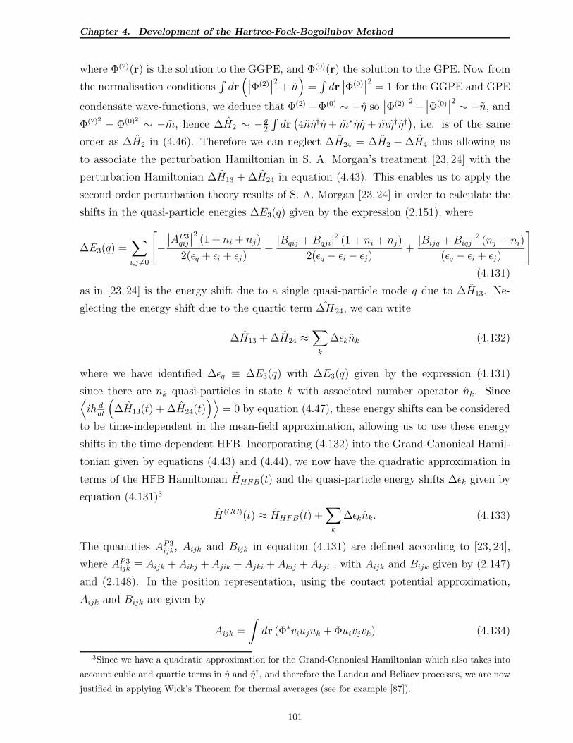
Chapter 4. Development of the Hartree-Fock-Bogoliubov Method
where Φ(2)(r) is the solution to the GGPE, and Φ(0)(r) the solution to the GPE. Now from
the normalisation conditions∫
dr(
∣
∣Φ(2)∣
∣
2+ n)
=∫
dr∣
∣Φ(0)∣
∣
2= 1 for the GGPE and GPE
condensate wave-functions, we deduce that Φ(2)−Φ(0) ∼ −η so∣
∣Φ(2)∣
∣
2−∣
∣Φ(0)∣
∣
2 ∼ −n, and
Φ(2)2 − Φ(0)2 ∼ −m, hence ∆H2 ∼ −g2
∫
dr(
4nη†η + m∗ηη + mη†η†)
, i.e. is of the same
order as ∆H2 in (4.46). Therefore we can neglect ∆H24 = ∆H2 + ∆H4 thus allowing us
to associate the perturbation Hamiltonian in S. A. Morgan’s treatment [23, 24] with the
perturbation Hamiltonian ∆H13 + ∆H24 in equation (4.43). This enables us to apply the
second order perturbation theory results of S. A. Morgan [23, 24] in order to calculate the
shifts in the quasi-particle energies ∆E3(q) given by the expression (2.151), where
∆E3(q) =∑
i,j 6=0
[
−∣
∣AP3qij
∣
∣
2(1 + ni + nj)
2(ǫq + ǫi + ǫj)+|Bqij +Bqji|2 (1 + ni + nj)
2(ǫq − ǫi − ǫj)+|Bijq +Biqj |2 (nj − ni)
(ǫq − ǫi + ǫj)
]
(4.131)
as in [23, 24] is the energy shift due to a single quasi-particle mode q due to ∆H13. Ne-
glecting the energy shift due to the quartic term ∆H24, we can write
∆H13 + ∆H24 ≈∑
k
∆ǫknk (4.132)
where we have identified ∆ǫq ≡ ∆E3(q) with ∆E3(q) given by the expression (4.131)
since there are nk quasi-particles in state k with associated number operator nk. Since⟨
i~ ddt
(
∆H13(t) + ∆H24(t))⟩
= 0 by equation (4.47), these energy shifts can be considered
to be time-independent in the mean-field approximation, allowing us to use these energy
shifts in the time-dependent HFB. Incorporating (4.132) into the Grand-Canonical Hamil-
tonian given by equations (4.43) and (4.44), we now have the quadratic approximation in
terms of the HFB Hamiltonian HHFB(t) and the quasi-particle energy shifts ∆ǫk given by
equation (4.131)3
H(GC)(t) ≈ HHFB(t) +∑
k
∆ǫknk. (4.133)
The quantities AP3ijk, Aijk and Bijk in equation (4.131) are defined according to [23, 24],
where AP3ijk ≡ Aijk + Aikj + Ajik + Ajki + Akij + Akji , with Aijk and Bijk given by (2.147)
and (2.148). In the position representation, using the contact potential approximation,
Aijk and Bijk are given by
Aijk =
∫
dr (Φ∗viujuk + Φuivjvk) (4.134)
3Since we have a quadratic approximation for the Grand-Canonical Hamiltonian which also takes into
account cubic and quartic terms in η and η†, and therefore the Landau and Beliaev processes, we are now
justified in applying Wick’s Theorem for thermal averages (see for example [87]).
101
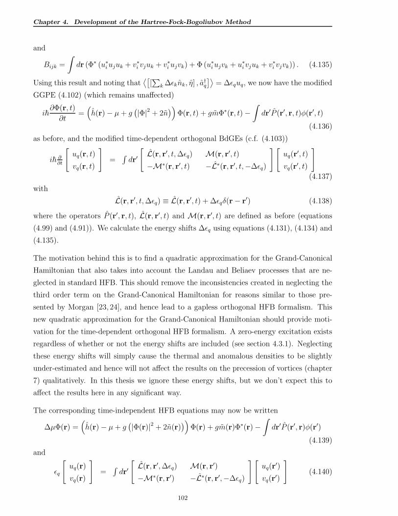
Chapter 4. Development of the Hartree-Fock-Bogoliubov Method
and
Bijk =
∫
dr (Φ∗ (u∗iujuk + v∗i vjuk + v∗i ujvk) + Φ (u∗iujvk + u∗i vjuk + v∗i vjvk)) . (4.135)
Using this result and noting that⟨[
[∑
k ∆ǫknk, η] , a†q
]⟩
= ∆ǫquq, we now have the modified
GGPE (4.102) (which remains unaffected)
i~∂Φ(r, t)
∂t=(
h(r)− µ+ g(
|Φ|2 + 2n)
)
Φ(r, t) + gmΦ∗(r, t)−∫
dr′P (r′, r, t)φ(r′, t)
(4.136)
as before, and the modified time-dependent orthogonal BdGEs (c.f. (4.103))
i~ ∂∂t
[
uq(r, t)
vq(r, t)
]
=∫
dr′
[
L(r, r′, t,∆ǫq) M(r, r′, t)
−M∗(r, r′, t) −L∗(r, r′, t,−∆ǫq)
][
uq(r′, t)
vq(r′, t)
]
(4.137)
with
L(r, r′, t,∆ǫq) ≡ L(r, r′, t) + ∆ǫqδ(r− r′) (4.138)
where the operators P (r′, r, t), L(r, r′, t) and M(r, r′, t) are defined as before (equations
(4.99) and (4.91)). We calculate the energy shifts ∆ǫq using equations (4.131), (4.134) and
(4.135).
The motivation behind this is to find a quadratic approximation for the Grand-Canonical
Hamiltonian that also takes into account the Landau and Beliaev processes that are ne-
glected in standard HFB. This should remove the inconsistencies created in neglecting the
third order term on the Grand-Canonical Hamiltonian for reasons similar to those pre-
sented by Morgan [23, 24], and hence lead to a gapless orthogonal HFB formalism. This
new quadratic approximation for the Grand-Canonical Hamiltonian should provide moti-
vation for the time-dependent orthogonal HFB formalism. A zero-energy excitation exists
regardless of whether or not the energy shifts are included (see section 4.3.1). Neglecting
these energy shifts will simply cause the thermal and anomalous densities to be slightly
under-estimated and hence will not affect the results on the precession of vortices (chapter
7) qualitatively. In this thesis we ignore these energy shifts, but we don’t expect this to
affect the results here in any significant way.
The corresponding time-independent HFB equations may now be written
∆µΦ(r) =(
h(r)− µ+ g(
|Φ(r)|2 + 2n(r))
)
Φ(r) + gm(r)Φ∗(r)−∫
dr′P (r′, r)φ(r′)
(4.139)
and
ǫq
[
uq(r)
vq(r)
]
=∫
dr′
[
L(r, r′,∆ǫq) M(r, r′)
−M∗(r, r′) −L∗(r, r′,−∆ǫq)
][
uq(r′)
vq(r′)
]
(4.140)
102
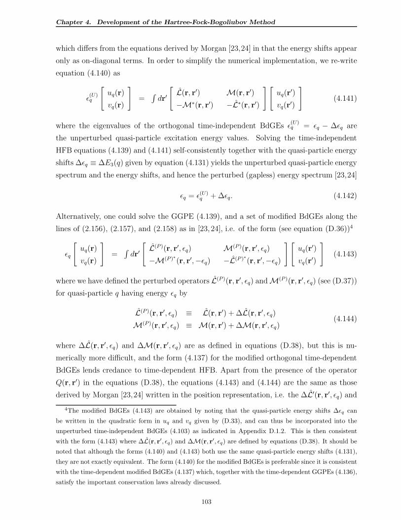
Chapter 4. Development of the Hartree-Fock-Bogoliubov Method
which differs from the equations derived by Morgan [23,24] in that the energy shifts appear
only as on-diagonal terms. In order to simplify the numerical implementation, we re-write
equation (4.140) as
ǫ(U)q
[
uq(r)
vq(r)
]
=∫
dr′
[
L(r, r′) M(r, r′)
−M∗(r, r′) −L∗(r, r′)
][
uq(r′)
vq(r′)
]
(4.141)
where the eigenvalues of the orthogonal time-independent BdGEs ǫ(U)q = ǫq − ∆ǫq are
the unperturbed quasi-particle excitation energy values. Solving the time-independent
HFB equations (4.139) and (4.141) self-consistently together with the quasi-particle energy
shifts ∆ǫq ≡ ∆E3(q) given by equation (4.131) yields the unperturbed quasi-particle energy
spectrum and the energy shifts, and hence the perturbed (gapless) energy spectrum [23,24]
ǫq = ǫ(U)q + ∆ǫq. (4.142)
Alternatively, one could solve the GGPE (4.139), and a set of modified BdGEs along the
lines of (2.156), (2.157), and (2.158) as in [23, 24], i.e. of the form (see equation (D.36))4
ǫq
[
uq(r)
vq(r)
]
=∫
dr′
[
L(P )(r, r′, ǫq) M(P )(r, r′, ǫq)
−M(P )∗(r, r′,−ǫq) −L(P )∗(r, r′,−ǫq)
][
uq(r′)
vq(r′)
]
(4.143)
where we have defined the perturbed operators L(P )(r, r′, ǫq) andM(P )(r, r′, ǫq) (see (D.37))
for quasi-particle q having energy ǫq by
L(P )(r, r′, ǫq) ≡ L(r, r′) + ∆L(r, r′, ǫq)
M(P )(r, r′, ǫq) ≡ M(r, r′) + ∆M(r, r′, ǫq)(4.144)
where ∆L(r, r′, ǫq) and ∆M(r, r′, ǫq) are as defined in equations (D.38), but this is nu-
merically more difficult, and the form (4.137) for the modified orthogonal time-dependent
BdGEs lends credance to time-dependent HFB. Apart from the presence of the operator
Q(r, r′) in the equations (D.38), the equations (4.143) and (4.144) are the same as those
derived by Morgan [23,24] written in the position representation, i.e. the ∆L′(r, r′, ǫq) and
4The modified BdGEs (4.143) are obtained by noting that the quasi-particle energy shifts ∆ǫq can
be written in the quadratic form in uq and vq given by (D.33), and can thus be incorporated into the
unperturbed time-independent BdGEs (4.103) as indicated in Appendix D.1.2. This is then consistent
with the form (4.143) where ∆L(r, r′, ǫq) and ∆M(r, r′, ǫq) are defined by equations (D.38). It should be
noted that although the forms (4.140) and (4.143) both use the same quasi-particle energy shifts (4.131),
they are not exactly equivalent. The form (4.140) for the modified BdGEs is preferable since it is consistent
with the time-dependent modified BdGEs (4.137) which, together with the time-dependent GGPEs (4.136),
satisfy the important conservation laws already discussed.
103
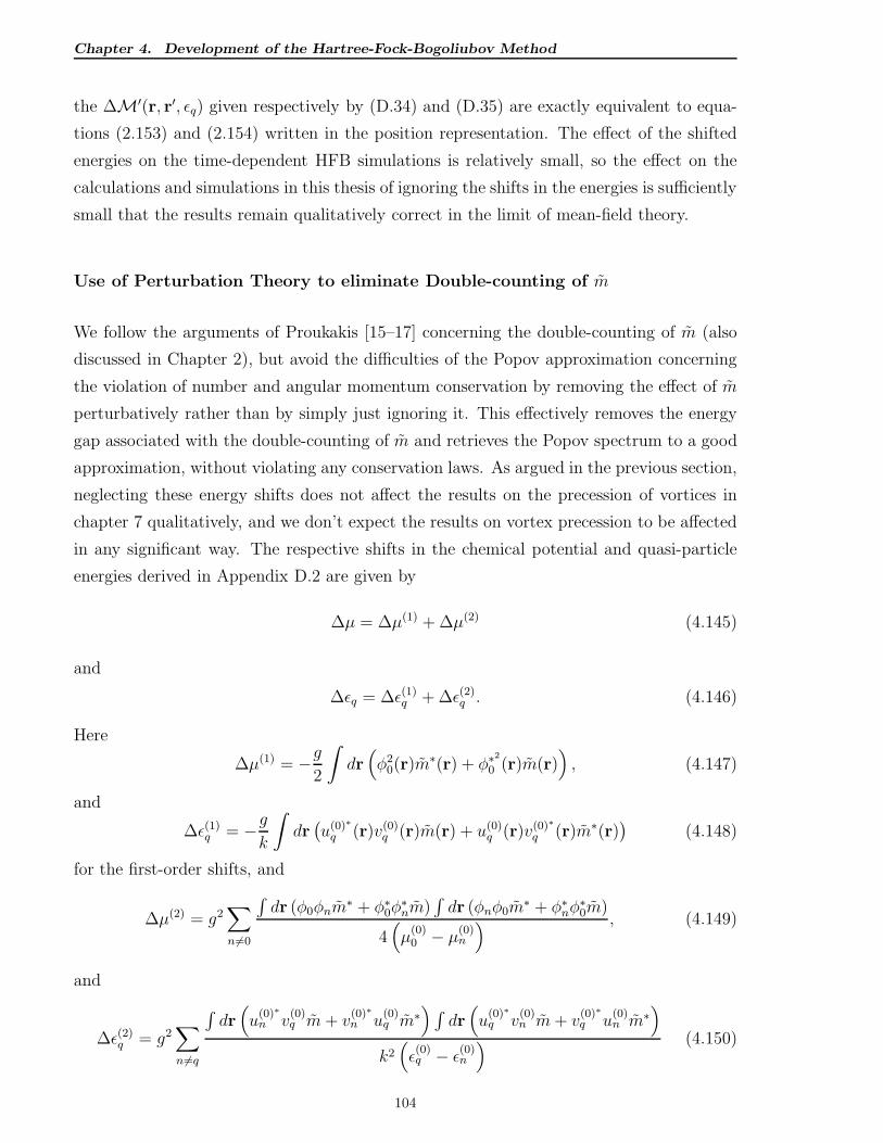
Chapter 4. Development of the Hartree-Fock-Bogoliubov Method
the ∆M′(r, r′, ǫq) given respectively by (D.34) and (D.35) are exactly equivalent to equa-
tions (2.153) and (2.154) written in the position representation. The effect of the shifted
energies on the time-dependent HFB simulations is relatively small, so the effect on the
calculations and simulations in this thesis of ignoring the shifts in the energies is sufficiently
small that the results remain qualitatively correct in the limit of mean-field theory.
Use of Perturbation Theory to eliminate Double-counting of m
We follow the arguments of Proukakis [15–17] concerning the double-counting of m (also
discussed in Chapter 2), but avoid the difficulties of the Popov approximation concerning
the violation of number and angular momentum conservation by removing the effect of m
perturbatively rather than by simply just ignoring it. This effectively removes the energy
gap associated with the double-counting of m and retrieves the Popov spectrum to a good
approximation, without violating any conservation laws. As argued in the previous section,
neglecting these energy shifts does not affect the results on the precession of vortices in
chapter 7 qualitatively, and we don’t expect the results on vortex precession to be affected
in any significant way. The respective shifts in the chemical potential and quasi-particle
energies derived in Appendix D.2 are given by
∆µ = ∆µ(1) + ∆µ(2) (4.145)
and
∆ǫq = ∆ǫ(1)q + ∆ǫ(2)q . (4.146)
Here
∆µ(1) = −g2
∫
dr(
φ20(r)m
∗(r) + φ∗2
0 (r)m(r))
, (4.147)
and
∆ǫ(1)q = −gk
∫
dr(
u(0)∗
q (r)v(0)q (r)m(r) + u(0)
q (r)v(0)∗
q (r)m∗(r))
(4.148)
for the first-order shifts, and
∆µ(2) = g2∑
n 6=0
∫
dr (φ0φnm∗ + φ∗
0φ∗nm)
∫
dr (φnφ0m∗ + φ∗
nφ∗0m)
4(
µ(0)0 − µ
(0)n
) , (4.149)
and
∆ǫ(2)q = g2∑
n 6=q
∫
dr(
u(0)∗
n v(0)q m+ v
(0)∗
n u(0)q m∗
)
∫
dr(
u(0)∗
q v(0)n m+ v
(0)∗
q u(0)n m∗
)
k2(
ǫ(0)q − ǫ(0)n
) (4.150)
104
Chapter 4. Development of the Hartree-Fock-Bogoliubov Method
for the second-order shifts. We apply these results by solving the GGPE (4.106), with
the shift in the chemical potential (4.145), the BdGEs (4.107) with the shifted chemical
potential, viz.
ǫq
[
uq(r)
vq(r)
]
=∫
dr′
[
L(r, r′,−∆µ) M(r, r′)
−M∗(r, r′) −L∗(r, r′,−∆µ)
][
uq(r′)
vq(r′)
]
(4.151)
with
L(r, r′,∆µ) ≡ L(r, r′) + ∆µδ(r− r′) (4.152)
(c.f. (4.138) and the energy shifts (4.146) self-consistently. This calculation does not
significantly increase the computational effort already required in solving the orthogonal
HFB equations, and reproduces the Popov quasi-particle energy spectrum to reasonable
accuracy (the errors are relatively small, typically ∼ 1 − 2%) and is therefore useful in
calculating the thermal densities more accurately.
Applicability of Perturbation Theory for Orthogonal HFB
In both perturbation techniques the quasi-particle energy spectrum is reproduced to rea-
sonable accuracy (< 5% in extreme cases). Since only the low-lying quasi-particle energies
are affected significantly by these calculations, the thermal densities may be calculated to
quite good accuracy in both cases5. In the parameter regime considered here, the differ-
ences due to the energy shifts are relatively small (typically 2 − 3%), and hence do not
significantly affect the results in this thesis. Calculations not presented here indicate that
the differences in the predicted transition temperature in the non-vortex case are also quite
small, with the transition temperature being slightly over-estimated in the unperturbed
case. They are in reasonable agreement with the Popov prediction which predicts a slightly
lower transition temperature. Further studies (also not presented here) indicate that the
Popov prediction for the vortex case under-estimates the transition temperature, whereas
the predictions for the unperturbed and perturbed orthogonal HFB calculations for the
vortex case remain in reasonable agreement, being slightly over-estimated in the unper-
turbed case. The predicted transition temperatures for the vortex case tend to be lower
than for the non-vortex case, but the Popov calculations produce predicted transition tem-
peratures that are unreasonably low in the vortex case. We conclude that the perturbation
5Some perturbation calculations using the perturbation scheme defined by equations (4.145)-(4.152)
have been performed for a BEC in the absence of any vortices for a mode cut-off of 209, and are presented
in appendix F.2.
105
Chapter 4. Development of the Hartree-Fock-Bogoliubov Method
calculations do not have a significant effect on either the thermal density or the predicted
transition temperature Tc.
In this way we justify the omission of perturbative calculations in the work done in this
thesis. The perturbative calculations could be included, but this would imply extra com-
putational effort which, in the light of the above discussion, is unnecessary for the purposes
of this thesis.
106
Chapter 5. Numerical Methods
Chapter 5
Numerical Methods
5.1 Introduction
In this chapter we present methods used to solve the time-independent and the time-
dependent orthogonal HFB equations1 in the regimes of axial symmetry and of tight axial
confinement. We also present methods of computing gradients accurately required for the
calculation of precessional frequencies of vortices using the continuity equation for the
condensate density. This is achieved by analytic differentiation and pre-calculation of the
first and second order partial derivatives of the Laguerre basis functions with respect to
the radial and azimuthal coordinates r and θ respectively. Before discussing the various
numerical techniques used, let us represent the orthogonal HFB equations in dimensionless
form.
1The numerical algorithms presented here relate to the orthogonal HFB formalism. It is easy, however,
to adapt these methods to standard HFB. In the numerical work done here, all time-independent calcu-
lations were done in the orthogonal formalism, whereas the time-dependent simulations were done mostly
using the standard HFB formalism to reduce the computational effort, and because this is also numerically
more robust. However, some of these calculations have been repeated using the orthogonal formalism, and
the differences found to be insignificant.
107
Chapter 5. Numerical Methods
5.2 Computational Units for BEC in Axially Sym-
metric Harmonic Trap
5.2.1 Computational Units for 3D system
We consider an axially symmetric harmonic trap, and define the length scale
r0 =
√
~
mωr(5.1)
and the time scale
t0 =2
ωr
(5.2)
so that the dimensionless forms (denoted by primes) now become
r = r0r′
t = t0t′.
(5.3)
It is also useful to use dimensionless forms for the condensate wave function, for the quasi-
particle amplitudes and for the condensate and non-condensate densities
Φ(r, t) =√
N/r30Φ
′(r, t)
uq(r, t) =√
N/r30u
′q(r, t)
vq(r, t) =√
N/r30v
′q(r, t)
(5.4)
Consequently
nc(r, t) = (N/r30)n
′c(r, t)
n(r, t) = (N/r30) n
′(r, t)
m(r, t) = (N/r30) m
′(r, t).
(5.5)
The energies are now given in harmonic oscillator units
E0 =~ωr
2. (5.6)
Thus we have, for example µ = E0µ′. Substituting (5.1) - (5.6) into the modified GGPE
(4.102), the BdGEs (4.103), and the expressions (4.5) and (4.99) for the operators L(r, t),
M(r, t), and P (r′, r, t), and dropping the primes denoting dimensionless units for notational
convenience, we obtain the dimensionless forms
i∂Φ(r, t)
∂t=(
h− µ+ C3D
(
|Φ|2 + 2n)
)
Φ(r, t) + C3DmΦ∗(r, t)−∫
dr′P (r′, r, t)φ(r′, t)
(5.7)
108
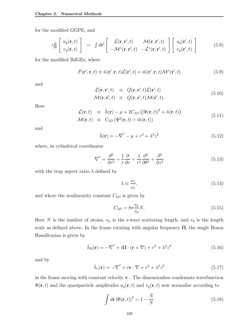
Chapter 5. Numerical Methods
for the modified GGPE, and
i ∂∂t
[
uq(r, t)
vq(r, t)
]
=∫
dr′
[
L(r, r′, t) M(r, r′, t)
−M∗(r, r′, t) −L∗(r, r′, t)
][
uq(r′, t)
vq(r′, t)
]
(5.8)
for the modified BdGEs, where
P (r′, r, t) ≡ n(r′, r, t)L(r′, t) + m(r′, r, t)M∗(r′, t) (5.9)
andL(r, r′, t) ≡ Q(r, r′, t)L(r′, t)
M(r, r′, t) ≡ Q(r, r′, t)M(r′, t).(5.10)
HereL(r, t) ≡ h(r)− µ+ 2C3D
(
|Φ(r, t)|2 + n(r, t))
M(r, t) ≡ C3D (Φ2(r, t) + m(r, t))(5.11)
and
h(r) = −∇2 − µ+ r2 + λ2z2 (5.12)
where, in cylindrical coordinates
∇2
=∂2
∂r2+
1
r
∂
∂r+
1
r2
∂2
∂θ2+
∂2
∂z2(5.13)
with the trap aspect ratio λ defined by
λ ≡ ωz
ωr, (5.14)
and where the nonlinearity constant C3D is given by
C3D = 8πas
r0N. (5.15)
Here N is the number of atoms, as is the s-wave scattering length, and r0 is the length
scale as defined above. In the frame rotating with angular frequency Ω, the single Boson
Hamiltonian is given by
hΩ(r) = −∇2
+ iΩ · (r×∇) + r2 + λ2z2 (5.16)
and by
hv(r) = −∇2
+ iv · ∇+ r2 + λ2z2 (5.17)
in the frame moving with constant velocity v . The dimensionless condensate wavefunction
Φ(r, t) and the quasiparticle amplitudes uq(r, t) and vq(r, t) now normalise according to
∫
dr |Φ(r, t)|2 = 1− N
N(5.18)
109
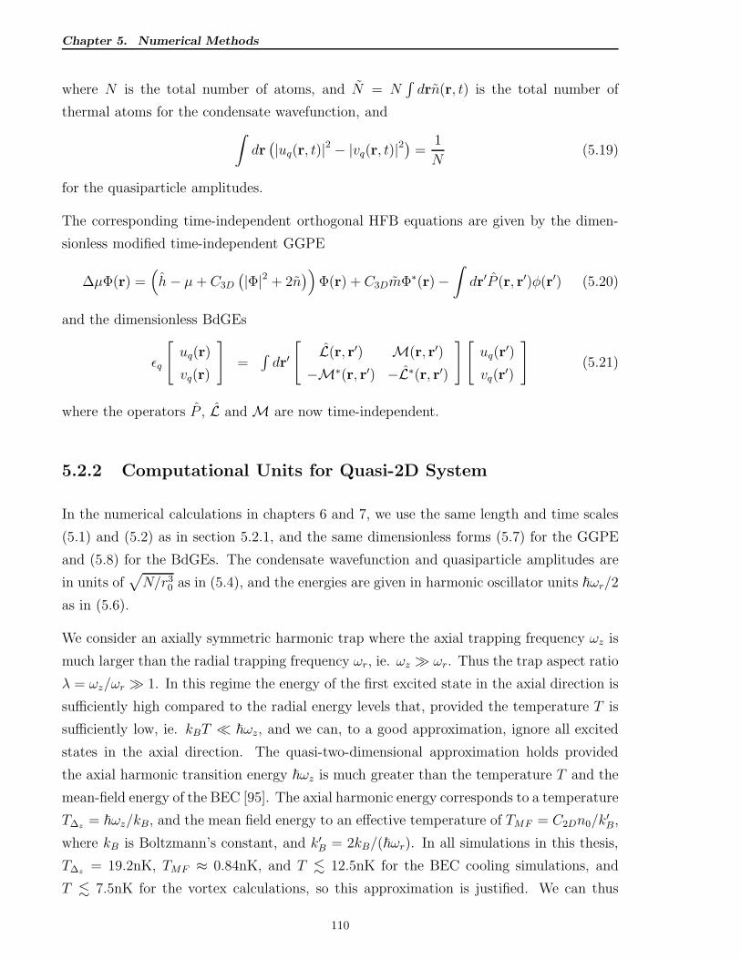
Chapter 5. Numerical Methods
where N is the total number of atoms, and N = N∫
drn(r, t) is the total number of
thermal atoms for the condensate wavefunction, and
∫
dr(
|uq(r, t)|2 − |vq(r, t)|2)
=1
N(5.19)
for the quasiparticle amplitudes.
The corresponding time-independent orthogonal HFB equations are given by the dimen-
sionless modified time-independent GGPE
∆µΦ(r) =(
h− µ+ C3D
(
|Φ|2 + 2n)
)
Φ(r) + C3DmΦ∗(r)−∫
dr′P (r, r′)φ(r′) (5.20)
and the dimensionless BdGEs
ǫq
[
uq(r)
vq(r)
]
=∫
dr′
[
L(r, r′) M(r, r′)
−M∗(r, r′) −L∗(r, r′)
][
uq(r′)
vq(r′)
]
(5.21)
where the operators P , L andM are now time-independent.
5.2.2 Computational Units for Quasi-2D System
In the numerical calculations in chapters 6 and 7, we use the same length and time scales
(5.1) and (5.2) as in section 5.2.1, and the same dimensionless forms (5.7) for the GGPE
and (5.8) for the BdGEs. The condensate wavefunction and quasiparticle amplitudes are
in units of√
N/r30 as in (5.4), and the energies are given in harmonic oscillator units ~ωr/2
as in (5.6).
We consider an axially symmetric harmonic trap where the axial trapping frequency ωz is
much larger than the radial trapping frequency ωr, ie. ωz ≫ ωr. Thus the trap aspect ratio
λ = ωz/ωr ≫ 1. In this regime the energy of the first excited state in the axial direction is
sufficiently high compared to the radial energy levels that, provided the temperature T is
sufficiently low, ie. kBT ≪ ~ωz, and we can, to a good approximation, ignore all excited
states in the axial direction. The quasi-two-dimensional approximation holds provided
the axial harmonic transition energy ~ωz is much greater than the temperature T and the
mean-field energy of the BEC [95]. The axial harmonic energy corresponds to a temperature
T∆z= ~ωz/kB, and the mean field energy to an effective temperature of TMF = C2Dn0/k
′B,
where kB is Boltzmann’s constant, and k′B = 2kB/(~ωr). In all simulations in this thesis,
T∆z= 19.2nK, TMF ≈ 0.84nK, and T . 12.5nK for the BEC cooling simulations, and
T . 7.5nK for the vortex calculations, so this approximation is justified. We can thus
110
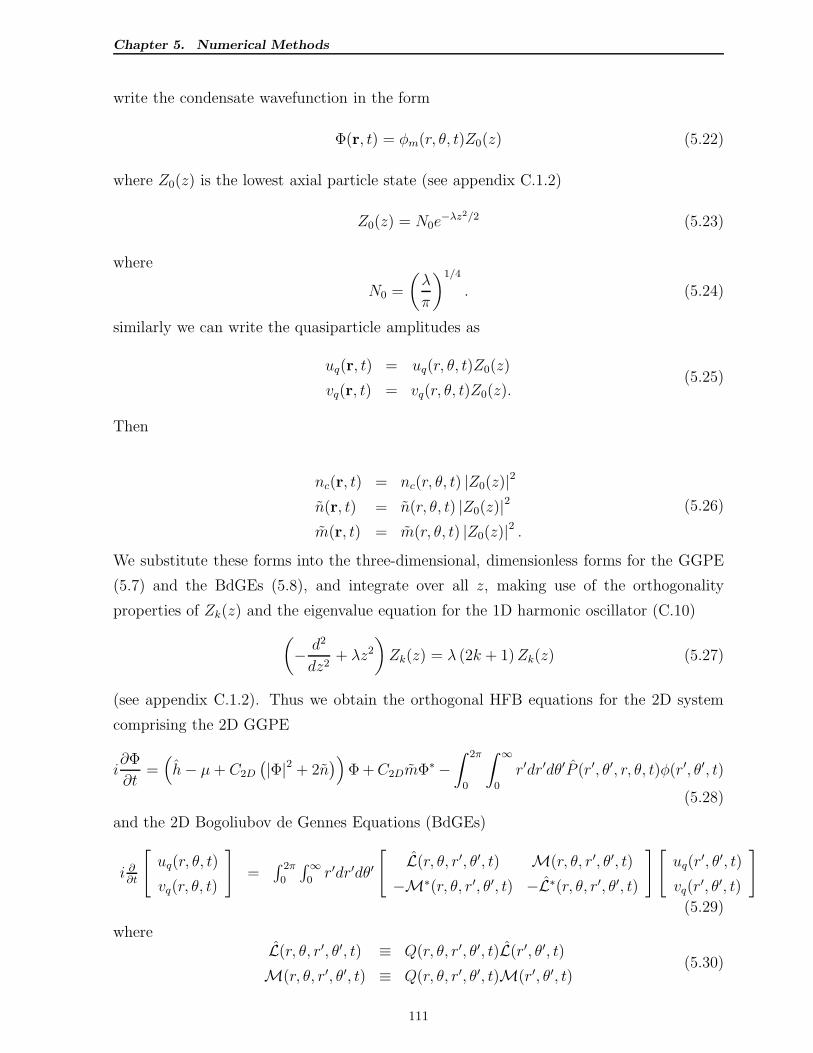
Chapter 5. Numerical Methods
write the condensate wavefunction in the form
Φ(r, t) = φm(r, θ, t)Z0(z) (5.22)
where Z0(z) is the lowest axial particle state (see appendix C.1.2)
Z0(z) = N0e−λz2/2 (5.23)
where
N0 =
(
λ
π
)1/4
. (5.24)
similarly we can write the quasiparticle amplitudes as
uq(r, t) = uq(r, θ, t)Z0(z)
vq(r, t) = vq(r, θ, t)Z0(z).(5.25)
Then
nc(r, t) = nc(r, θ, t) |Z0(z)|2
n(r, t) = n(r, θ, t) |Z0(z)|2
m(r, t) = m(r, θ, t) |Z0(z)|2 .(5.26)
We substitute these forms into the three-dimensional, dimensionless forms for the GGPE
(5.7) and the BdGEs (5.8), and integrate over all z, making use of the orthogonality
properties of Zk(z) and the eigenvalue equation for the 1D harmonic oscillator (C.10)
(
− d2
dz2+ λz2
)
Zk(z) = λ (2k + 1)Zk(z) (5.27)
(see appendix C.1.2). Thus we obtain the orthogonal HFB equations for the 2D system
comprising the 2D GGPE
i∂Φ
∂t=(
h− µ+ C2D
(
|Φ|2 + 2n)
)
Φ +C2DmΦ∗−∫ 2π
0
∫ ∞
0
r′dr′dθ′P (r′, θ′, r, θ, t)φ(r′, θ′, t)
(5.28)
and the 2D Bogoliubov de Gennes Equations (BdGEs)
i ∂∂t
[
uq(r, θ, t)
vq(r, θ, t)
]
=∫ 2π
0
∫∞0r′dr′dθ′
[
L(r, θ, r′, θ′, t) M(r, θ, r′, θ′, t)
−M∗(r, θ, r′, θ′, t) −L∗(r, θ, r′, θ′, t)
][
uq(r′, θ′, t)
vq(r′, θ′, t)
]
(5.29)
whereL(r, θ, r′, θ′, t) ≡ Q(r, θ, r′, θ′, t)L(r′, θ′, t)
M(r, θ, r′, θ′, t) ≡ Q(r, θ, r′, θ′, t)M(r′, θ′, t)(5.30)
111
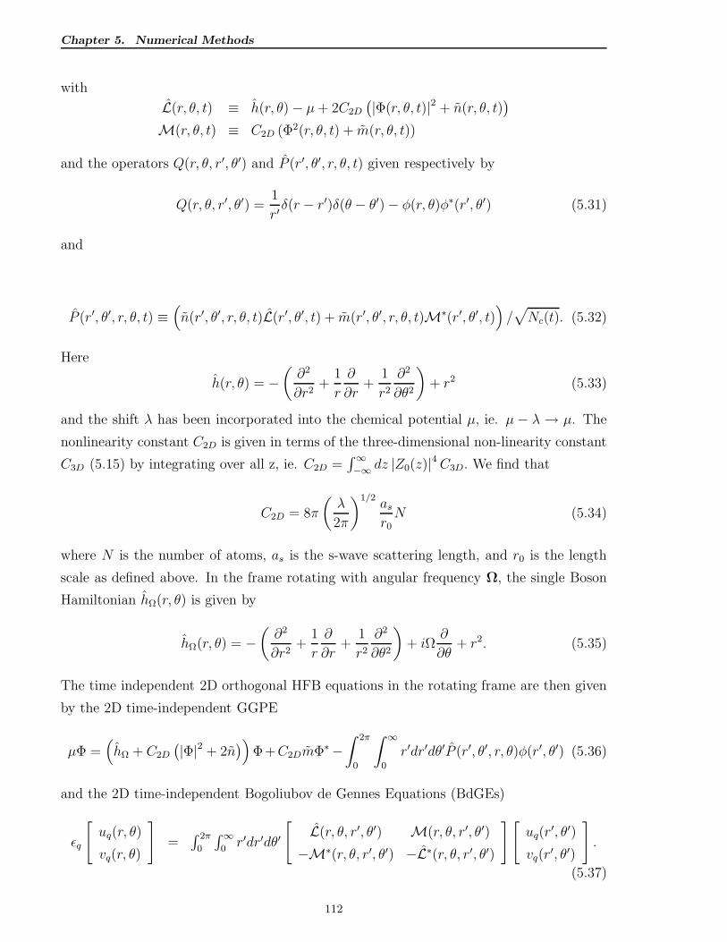
Chapter 5. Numerical Methods
with
L(r, θ, t) ≡ h(r, θ)− µ+ 2C2D
(
|Φ(r, θ, t)|2 + n(r, θ, t))
M(r, θ, t) ≡ C2D (Φ2(r, θ, t) + m(r, θ, t))
and the operators Q(r, θ, r′, θ′) and P (r′, θ′, r, θ, t) given respectively by
Q(r, θ, r′, θ′) =1
r′δ(r − r′)δ(θ − θ′)− φ(r, θ)φ∗(r′, θ′) (5.31)
and
P (r′, θ′, r, θ, t) ≡(
n(r′, θ′, r, θ, t)L(r′, θ′, t) + m(r′, θ′, r, θ, t)M∗(r′, θ′, t))
/√
Nc(t). (5.32)
Here
h(r, θ) = −(
∂2
∂r2+
1
r
∂
∂r+
1
r2
∂2
∂θ2
)
+ r2 (5.33)
and the shift λ has been incorporated into the chemical potential µ, ie. µ − λ → µ. The
nonlinearity constant C2D is given in terms of the three-dimensional non-linearity constant
C3D (5.15) by integrating over all z, ie. C2D =∫∞−∞ dz |Z0(z)|4C3D. We find that
C2D = 8π
(
λ
2π
)1/2as
r0N (5.34)
where N is the number of atoms, as is the s-wave scattering length, and r0 is the length
scale as defined above. In the frame rotating with angular frequency Ω, the single Boson
Hamiltonian hΩ(r, θ) is given by
hΩ(r, θ) = −(
∂2
∂r2+
1
r
∂
∂r+
1
r2
∂2
∂θ2
)
+ iΩ∂
∂θ+ r2. (5.35)
The time independent 2D orthogonal HFB equations in the rotating frame are then given
by the 2D time-independent GGPE
µΦ =(
hΩ + C2D
(
|Φ|2 + 2n)
)
Φ+C2DmΦ∗−∫ 2π
0
∫ ∞
0
r′dr′dθ′P (r′, θ′, r, θ)φ(r′, θ′) (5.36)
and the 2D time-independent Bogoliubov de Gennes Equations (BdGEs)
ǫq
[
uq(r, θ)
vq(r, θ)
]
=∫ 2π
0
∫∞0r′dr′dθ′
[
L(r, θ, r′, θ′) M(r, θ, r′, θ′)
−M∗(r, θ, r′, θ′) −L∗(r, θ, r′, θ′)
][
uq(r′, θ′)
vq(r′, θ′)
]
.
(5.37)
112
Chapter 5. Numerical Methods
5.3 Numerical Solutions of the Time-independent HFB
Equations
The regime of interest here is the axially symmetric harmonically confined quasi-2D BEC
(tight axial confinement). We shall consider the cases of an axially symmetric BEC in
the absence of vortices, or with a single on-axis vortex, and the more general non-axially-
symmetric BEC (which may have several off-axis vortices). In the former case, the az-
imuthal coordinate θ may be integrated out producing a set of radial HFB equations, and
in the second case we have a two dimensional set of equations in the radial coordinate r
and the azimuthal coordinate θ. In both cases the axial confinement is considered to be
sufficiently strong such that all excitations in the axial direction may be ignored, and the
axial coordinate z integrated out to produce a one or a two-dimensional problem with a
suitably modified non-linearity parameter - see section 5.2.2.
In all cases we expand the condensate wave-function Φ(r) and the quasi-particle amplitudes
uq(r) and vq(r) in terms of the single-particle basis functions ξk(r). These single-particle
basis functions are solutions of the (single-particle) time-independent Schrodinger equation
with respective energy eigenvalues µ(SP )k , viz.
µ(SP )k ξk(r) = h(r)ξk(r) (5.38)
Thus we may write the condensate wave function Φ(r) as
Φ(r) =∑
k
a0kξk(r) (5.39)
and the quasiparticle amplitudes uq(r) and vq(r) as
uq(r) =∑
k
cqkξk(r) (5.40)
and
vq(r) =∑
k
dqkξk(r) (5.41)
respectively. In this way we obtain matrix (eigenvalue) equations for the coefficients ajk for
the condensate wave-function Φ(r) (we use the lowest energy eigenvector for condensate
wave-function, and hence the coefficients a0k), and for the coefficients cqk and dqk for
the quasi-particle amplitudes uq(r) and vq(r) written in terms of the respective matrix
elements. We obtain the following matrix equations. For the coefficients for the condensate
wavefunction (GGPE) we obtain (see appendix C.2.1)
µa = (A + B)a (5.42)
113
Chapter 5. Numerical Methods
and for the quasiparticle amplitudes (BdGEs) the matrix equation
ǫq
[
cq
dq
]
=
[
L(u)q M
(u)q
−M(v)q −L
(v)q
][
cq
dq
]
. (5.43)
The matrices A, B, L(u)q , M
(u)q , L
(v)q , and M
(v)q represent the matrix elements of the GGPE
and the BdGEs respectively, and are defined in appendix C.2.1. In the laboratory (LAB)
frame in the axially symmetric case and in the absence of any vortices, we have L(u)q = L
(v)q
and M(u)q = M
(v)q , but this is not the case in general.
5.3.1 Numerical Solutions for the Quasi-2D BEC
In all cases, we assume axial symmetry of the confining potential. We also assume tight
axial confinerment (ωr ≫ ωz) such that we can ignore all excitations in the axial direction,
thus allowing the z-coordinate to be integrated out, yielding the 2D time-independent
orthogonal HFB equations comprising the 2D time-independent GGPE (5.36) and the 2D
time-independent orthogonal BdGEs (5.37) . In the rotating frame the angular precessional
frequency for off-axis vortices may be calculated using equation (4.65). We now consider
the cases of no vortices, a single on-axis vortex, and of one or more off-axis vortices. In all
cases we expand the condensate wave-function Φ(r, θ) and the quasi-particle amplitudes
uq(r1, θ1) and vq(r1, θ1) in terms of the single-particle basis functions ξln(r, θ) satisfying the
single-particle Schrodinger equation
µ(SP )ln ξln(r, θ) = h(r, θ)ξln(r, θ). (5.44)
These are simply the Laguerre basis functions
ξln(r, θ), l = 0,±1, . . . , n = 0, 1, . . .
de-
fined by (C.26)
ξln(r, θ) = ξln(r)eilθ
√2π
(5.45)
where the radial Laguerre function is given by
ξln(r) =
(
2n!
(n+ |l|)!
)1/2
e−r2/2r|l|L|l|n (r2) (5.46)
and where the L|l|n (r2) are nth order modified Laguerre polynomials in r2.
Axially-symmetric Solutions
In the case of axial symmetry of the solutions, we can integrate out the azimuthal coordinate
θ (see also section 7.2, chapter 7 and section C.2.2 of the appendix) to obtain the radial
114
Chapter 5. Numerical Methods
time-independent orthogonal HFB equations comprised of the radial time-independent
GGPE
∆µΦ(r) =(
hm,Ω(r)− µ+ CR2D
(
|Φ(r)|2 + 2n(r))
)
Φ(r)+CR2Dm(r)Φ(r)−
∫ ∞
0
r′dr′P (r′, r)φ(r′)
(5.47)
and the radial time-independent orthogonal BdGEs
ǫlq
[
ulq(r)
vlq(r)
]
=∫∞0r′dr′
[
Ql(r, r′)Ll+m(r′) Ql(r, r
′)M(r′)
−Ql(r, r′)M(r′) −Ql(r, r
′)Ll−m(r′)
][
ulq(r′)
vlq(r′)
]
,
(5.48)
where we have defined the radial operators Ll(r) ,M(r)
Ll(r) ≡ hl(r)− µ+ 2CR2D
(
|Φ(r)|2 + n(r))
M(r) ≡ CR2D (Φ2(r) + m(r))
(5.49)
and the operator P (r′, r)
P (r′, r) ≡(
n(r′, r)L(r′) + m(r′, r)M∗(r′))
/√
Nc(t) (5.50)
with the single-particle Hamiltonian in the LAB frame given by
hl(r) ≡ −(
d2
dr2+
1
r
d
dr
)
+l2
r2− µ+ r2, (5.51)
and by
hl,Ω(r) ≡ −(
d2
dr2+
1
r
d
dr
)
+l2
r2− lΩ + r2 (5.52)
in the rotating frame. The radial projection operator Q(r, r1) is given by
Ql(r, r′) = δ(r, r′)− δl,0φ(r)φ(r′), (5.53)
and the radial 2D nonlinearity constant CR2D ≡ C2D/2π by
CR2D = 4
(
λ
2π
)1/2as
r0N. (5.54)
In this case we can expand the radial condensate wave-function Φ(r) and the radial quasi-
particle amplitudes ulq(r) and vlq(r) in terms of the radial Laguerre basis functions ξln(r),
i.e.
Φ(r) =∑
n
a0,mnξmn(r) (5.55)
for the condensate wave-function, and
uq(r) =∑
ln
cq,lnξl+m,n(r) (5.56)
115
Chapter 5. Numerical Methods
and
vq(r) =∑
ln
dq,lnξl−m,n(r) (5.57)
for the quasi-particle amplitudes. Here we have allowed for the existence of an on-axis vor-
tex of vorticity m . In the case of no vortices, m = 0 . Thus we obtain the vector eigenvalue
equation for the coefficients for the condensate wavefunction (GGPE) and for the quasipar-
ticle amplitudes (BdGEs) given respectively by equations of the form (5.42) and (5.43) as
before (see appendix C.2.2). We note that the radial Laguerre basis functions ξln(r) given
by equation (5.46) may be written as a polynomial of order n + l in r2 times a weighting
factor exp (−r2/2), thus all matrix elements are integrals of orthogonal polynomials of or-
der 4N +2M−4 in r2 (since dr2 = 2rdr), where we have imposed the computational mode
cut-off of n = 0, . . . , N − 1 and l = 0,±1, . . . ,±M. This facilitates the use of Gaus-
sian quadrature for the integration (see section (5.5)), allowing accurate computation for
a minimal number of position points, greatly enhancing the efficiency and accuracy of the
numerical algorithms used here.
Single Off-axis Vortex
We find stationary solutions for a single off-axis vortex by solving the 2D orthogonal HFB
equations (5.36) and (5.37), and the equation for the precessional frequency (4.65) self-
consistently with C(r, θ) given by (4.125). We can write the condensate wave function
Φ(r, θ) in in the Laguerre basis ξln(r, θ)
Φ(r, θ) =∑
ln
alnξln(r, θ) (5.58)
and similarly the quasi-particle amplitudes uq(r, θ), vq(r, θ)
uq(r, θ) =∑
ln
cq,lnξln(r, θ) (5.59)
and
vq(r, θ) =∑
ln
dq,lnξln(r, θ). (5.60)
Suppose we have a single vortex situated at position (r1, θ1) such that (r1, θ1) does not lie
on any of the roots of the Laguerre basis functions ξln(r, θ). Then
Φ(r1, θ1) =∑
ln
alnξln(r1, θ1) = 0 (5.61)
so
a10 = −∑
l,n∈S(1)
alnξln(r1, θ1)
ξ10(r1, θ1)(5.62)
116
Chapter 5. Numerical Methods
gives the necessary constraint for the vortex to be at this position, where we have defined
S(1) ≡ l, n | (l, n) ∈ S − (1, 0) (5.63)
where S ≡ l, n | n = 0, . . . , l = 0,±1, . . . in anticipation of an iteration formula for the
case of multiple vortices. Then we can write
Φ(r, θ) =∑
l,n∈S(1)
alnχ(1)ln (r, θ) (5.64)
where we have defined the modified basis functions
χ(1)ln (r, θ) ≡ ξln(r, θ)−
ξln(r1, θ1)
ξ10(r1, θ1)ξ10(r, θ) (5.65)
corresponding to a single vortex situated at (r1, θ1). Substituting (5.64) into the GGPE
(5.36), and (5.59),(5.60) into the orthogonal BdGEs (5.37), and making use of the fact that
∞∫
0
2π∫
0
rdrdθξ∗ln(r, θ)χ(1)l′n′(r, θ) = δl,l′δn,n′ (5.66)
we again obtain the matrix equations for the coefficients for the condensate wavefunction
(GGPE) and for the quasiparticle amplitudes (BdGEs) given by the vector equations of
the form (5.42) and (5.43) (see appendix C.2.3).
Multiple Vortices
This procedure may be extended toNv vortices situated at positions (r, θ) ∈ (ri, θi) | i = 1, . . .Nvby an iterative process. Let us extend the notation (5.63) for Nv vortices, and define
S(Nv) ≡ l, n | (l, n) ∈ S − (1, 0) , . . . , (Nv, 0) . (5.67)
Then suppose that for Nv − 1 vortices we can write
Φ(r, θ) =∑
l,n∈S(Nv−1)
alnχ(Nv−1)ln (r, θ) (5.68)
where the modified basis function for Nv − 1 vortices is given by
χ(Nv−1)ln (r, θ) ≡ χ
(Nv−2)ln (r, θ)− χ
(Nv−2)ln (rNv−1, θNv−1)
χ(Nv−2)Nv−1,0(rNv−1, θNv−1)
χ(Nv−2)Nv−1,0(r, θ)
Then introducing another vortex Nv at position (rNv, θNv
) implies
Φ(rNv, θNv
) =∑
l,n∈S(Nv)
alnχ(Nv)ln (rNv
, θNv) = 0
117
Chapter 5. Numerical Methods
hence
aNv−1,0 = −∑
l,n∈S(Nv−1)
alnχ
(Nv−1)ln (rNv
, θNv)
χ(Nv−1)00 (rNv
, θNv)
so that for Nv vortices
Φ(r, θ) =∑
l,n∈S(Nv)
alnχ(Nv)ln (r, θ) (5.69)
where we define the modified basis functions
χ(Nv)ln (r, θ) ≡ χ
(Nv−1)ln (r, θ)− χ
(Nv−1)ln (rNv
, θNv)
χ(Nv−1)Nv0 (rNv
, θNv)χ
(Nv−1)Nv0 (r, θ) (5.70)
for Nv vortices situated at (r, θ) ∈ (ri, θi) | i = 1, . . . Nv. Further it can be shown that
that∞∫
0
2π∫
0
rdrdθξ∗ln(r, θ)χ(Nv)l′n′ (r, θ) = δll′δnn′ (5.71)
permitting us to write the vector equations for the coefficients for the condensate wavefunc-
tion (GGPE) and for the quasiparticle amplitudes (BdGEs) in the form given respectively
by equations (5.42) and (5.43) as before (see appendix C.2.3).
Numerical Calculation of the Precessional Frequency Ω
We use equation (4.65) with C(r, θ) given by (4.125) to calculate the precessional frequency
Ω in the case of single and multiple off-axis vortices. Let R = Re Φ and I = Im Φrepresent respectively the real and imaginary parts of the condensate wavefunction, then
Φ(r, t) = R(r, t) + iI(r, t). (5.72)
Calculation of the precessional frequency Ω requires numerical computation of the quan-
tities r ∂∂r
Φ(r, θ), r2 ∂2
∂r2 Φ(r, θ), ∂∂θ
Φ(r, θ), and ∂2
∂θ2 Φ(r, θ) involving first and second order
derivatives of the condensate function Φ given by equations (C.115)-(C.118). The deriva-
tives of the modified basis functions are found analytically using the recurrence relations of
the Laguerre basis functions, and the iterative relations (5.65) and (5.70) for the modified
basis functions for single and multiple vortices. This permits accurate computation of the
derivatives (C.115)-(C.118), in contrast to numeric differentiation which would be very
inaccurate for the Gaussian grid used here, and which would be very sensitive to numerical
noise.
Using the recurrence relation [103,104]
rdLk
n(r)
dr= nLk
n(r)− (n+ k)Lkn−1(r) (5.73)
118
Chapter 5. Numerical Methods
for the generalised associated Laguerre polynomial Lkn(r), and the expression (5.46) for the
radial Laguerre basis function ξln(r) = N|l|n e−r2/2r|l|L
|l|n (r2) , we find that
rdξln(r)
dr=(
2n + |l| − r2)
ξln(r)− 2√
n (n + |l|)ξl,n−1(r) (5.74)
and
r2d2ξln(r)
dr2=(
2n+ |l| − 1− r2)
rdξln(r)
dr− 2r2ξln(r)− 2
√
n (n+ |l|)rdξl,n−1(r)
dr. (5.75)
By (5.45) we have
∂ξln(r, θ)
∂θ= ilξln(r, θ) (5.76)
and∂2ξln(r, θ)
∂θ2= −l2ξln(r, θ). (5.77)
This allows us to calculate the derivatives of the basis functions, and hence of the modified
basis functions analytically. For a single vortex, the quantities r ∂∂rχ
(1)ln (r, θ), r2 ∂2
∂r2χ(1)ln (r, θ),
∂∂θχ
(1)ln (r, θ) and ∂2
∂θ2χ(1)ln (r, θ) for the modified Laguerre basis functions are given by equations
(C.124)-(C.127). By a process of iteration one can calculate the derivatives in the case of
any number of vortices Nv by use of the equations (C.128)-(C.131) which follow directly
from the iterative formula (5.70).
These derivatives for the modified Laguerre basis functions are pre-calculated (as are all
basis functions used in these calculations), thus greatly enhancing performance.
5.4 Numerical Solution of the Time-dependent HFB
Equations
We discuss two methods here for the solution of the time-dependent orthogonal HFB
equations. The first method is the fourth-order Runge-Kutta interaction-picture (RK4IP)
algorithm that uses fast Fourier transforms and inverse transforms, and the fourth-order
Runge-Kutta numerical integration algorithm to solve the HFB equations in the interaction
picture. The second is an algorithm where the wave-function and quasi-particle amplitudes
are represented in the Laguerre basis, and a fourth-order Runge-Kutta algorithm used
to determine the time evolution of the condensate wave-function and the quasi-particle
amplitude coefficients.
119
Chapter 5. Numerical Methods
5.4.1 Brief Description of the RK4IP Algorithm [90]
We consider a matrix differential equation of the form
∂Ψ(r, t)
∂t= DΨ(r, t) + G(Ψ(r, t), r, t)Ψ(r, t) (5.78)
where Ψ(r, t) is a vector wave function, D is a matrix differential operator with character-
istic equation d(α) (eg. for D = ∇2, d(−2πik) = |−2πik|2), and G(Ψ(r, t), r, t) a matrix
function of the vector wave-function Ψ(r, t), and of position r and time t. We shall see
presently how the time-dependent HFB equations can be cast in this form. We define the
interaction picture wavefunction vector ΨI(r, t) given by
ΨI(r, t) = exp (−D(t− ξ))Ψ(r, t) (5.79)
Then
∂ΨI(r, t)
∂t= exp (−D(t− ξ))G(Ψ(r, t), r, t)Ψ(r, t) = f
(
ΨI(r, t), r, t)
(5.80)
where we define the vector function
f(
ΨI(r, t), r, t)
= exp (−D(t− ξ))G(Ψ(r, t), r, t)Ψ(r, t) (5.81)
for some arbitrary parameter ξ, which we will choose later in such a way as to optimise
the algorithm. Using the fourth order Runge-Kutta algorithm (see for example [91]), we
integrate this equation numerically. The value of ΨI(r, t), the vector wavefunction in the
interaction picture at the (n + 1)th step is given by
ΨI(r, tn+1) = ΨI(r, tn) + [k1 + 2 (k2 + k3) + k4] /6 (5.82)
where
k1 = f(
ΨI(r, tn), r, tn)
∆t (5.83)
k2 = f
(
ΨI(r, tn +∆t
2) +
k1
2, r, tn +
∆t
2
)
∆t (5.84)
k3 = f
(
ΨI(r, tn +∆t
2) +
k2
2, r, tn +
∆t
2
)
∆t (5.85)
k4 = f(
ΨI(r, tn + ∆t) + k3, r, tn + ∆t)
∆t (5.86)
where we have defined the function f(
ΨI(r, t), r, t)
as above (5.81). This Runge-Kutta
step advances ΨI(r, tn)→ ΨI(r, tn+1). We can evaluate f(
ΨI(r, t), r, t)
from (5.81) using
the Fourier transform technique, we find that
f(
ΨI(r, t), r, t)
= F−1k Fr G(Ψ(r, t), r, t)Ψ(r, t) exp (−d(−2πik) (t− ξ) (5.87)
120
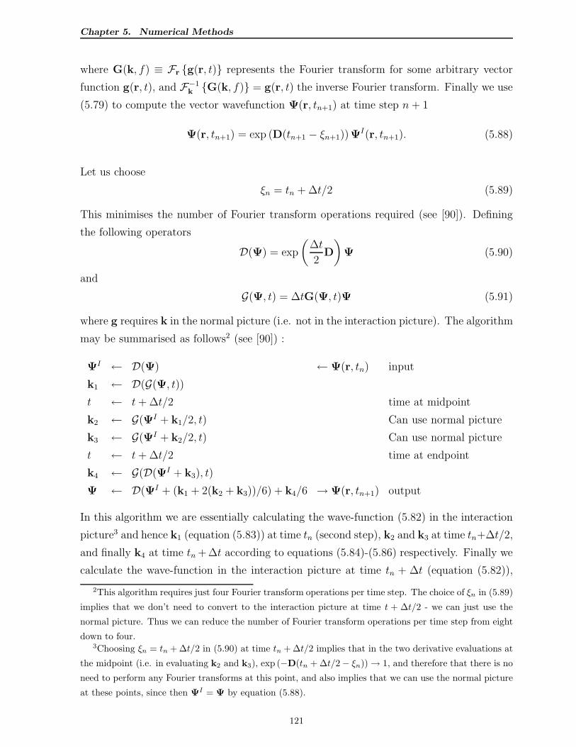
Chapter 5. Numerical Methods
where G(k, f) ≡ Fr g(r, t) represents the Fourier transform for some arbitrary vector
function g(r, t), and F−1k G(k, f) = g(r, t) the inverse Fourier transform. Finally we use
(5.79) to compute the vector wavefunction Ψ(r, tn+1) at time step n + 1
Ψ(r, tn+1) = exp (D(tn+1 − ξn+1))ΨI(r, tn+1). (5.88)
Let us choose
ξn = tn + ∆t/2 (5.89)
This minimises the number of Fourier transform operations required (see [90]). Defining
the following operators
D(Ψ) = exp
(
∆t
2D
)
Ψ (5.90)
and
G(Ψ, t) = ∆tG(Ψ, t)Ψ (5.91)
where g requires k in the normal picture (i.e. not in the interaction picture). The algorithm
may be summarised as follows2 (see [90]) :
ΨI ← D(Ψ) ← Ψ(r, tn) input
k1 ← D(G(Ψ, t))t ← t+ ∆t/2 time at midpoint
k2 ← G(ΨI + k1/2, t) Can use normal picture
k3 ← G(ΨI + k2/2, t) Can use normal picture
t ← t+ ∆t/2 time at endpoint
k4 ← G(D(ΨI + k3), t)
Ψ ← D(ΨI + (k1 + 2(k2 + k3))/6) + k4/6 → Ψ(r, tn+1) output
In this algorithm we are essentially calculating the wave-function (5.82) in the interaction
picture3 and hence k1 (equation (5.83)) at time tn (second step), k2 and k3 at time tn+∆t/2,
and finally k4 at time tn +∆t according to equations (5.84)-(5.86) respectively. Finally we
calculate the wave-function in the interaction picture at time tn + ∆t (equation (5.82)),
2This algorithm requires just four Fourier transform operations per time step. The choice of ξn in (5.89)
implies that we don’t need to convert to the interaction picture at time t + ∆t/2 - we can just use the
normal picture. Thus we can reduce the number of Fourier transform operations per time step from eight
down to four.3Choosing ξn = tn + ∆t/2 in (5.90) at time tn + ∆t/2 implies that in the two derivative evaluations at
the midpoint (i.e. in evaluating k2 and k3), exp (−D(tn + ∆t/2− ξn))→ 1, and therefore that there is no
need to perform any Fourier transforms at this point, and also implies that we can use the normal picture
at these points, since then ΨI = Ψ by equation (5.88).
121
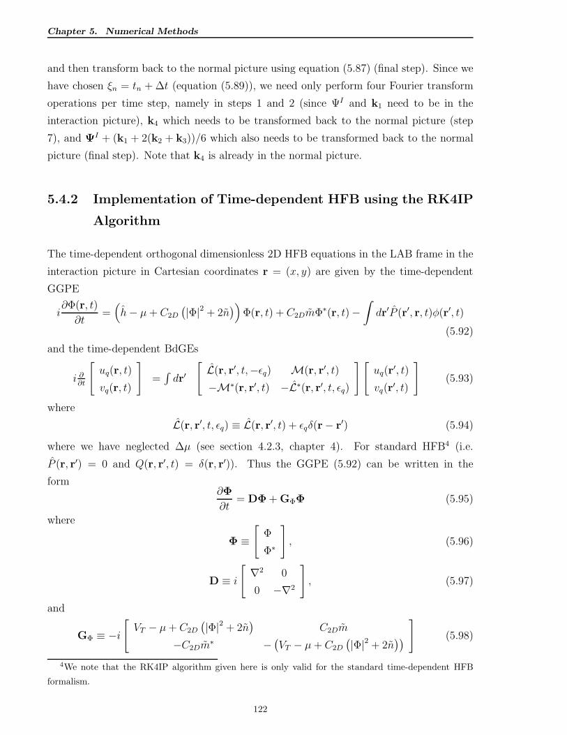
Chapter 5. Numerical Methods
and then transform back to the normal picture using equation (5.87) (final step). Since we
have chosen ξn = tn + ∆t (equation (5.89)), we need only perform four Fourier transform
operations per time step, namely in steps 1 and 2 (since ΨI and k1 need to be in the
interaction picture), k4 which needs to be transformed back to the normal picture (step
7), and ΨI + (k1 + 2(k2 + k3))/6 which also needs to be transformed back to the normal
picture (final step). Note that k4 is already in the normal picture.
5.4.2 Implementation of Time-dependent HFB using the RK4IP
Algorithm
The time-dependent orthogonal dimensionless 2D HFB equations in the LAB frame in the
interaction picture in Cartesian coordinates r = (x, y) are given by the time-dependent
GGPE
i∂Φ(r, t)
∂t=(
h− µ+ C2D
(
|Φ|2 + 2n)
)
Φ(r, t) + C2DmΦ∗(r, t)−∫
dr′P (r′, r, t)φ(r′, t)
(5.92)
and the time-dependent BdGEs
i ∂∂t
[
uq(r, t)
vq(r, t)
]
=∫
dr′
[
L(r, r′, t,−ǫq) M(r, r′, t)
−M∗(r, r′, t) −L∗(r, r′, t, ǫq)
][
uq(r′, t)
vq(r′, t)
]
(5.93)
where
L(r, r′, t, ǫq) ≡ L(r, r′, t) + ǫqδ(r− r′) (5.94)
where we have neglected ∆µ (see section 4.2.3, chapter 4). For standard HFB4 (i.e.
P (r, r′) = 0 and Q(r, r′, t) = δ(r, r′)). Thus the GGPE (5.92) can be written in the
form∂Φ
∂t= DΦ + GΦΦ (5.95)
where
Φ ≡[
Φ
Φ∗
]
, (5.96)
D ≡ i
[
∇2 0
0 −∇2
]
, (5.97)
and
GΦ ≡ −i[
VT − µ+ C2D
(
|Φ|2 + 2n)
C2Dm
−C2Dm∗ −
(
VT − µ+ C2D
(
|Φ|2 + 2n))
]
(5.98)
4We note that the RK4IP algorithm given here is only valid for the standard time-dependent HFB
formalism.
122
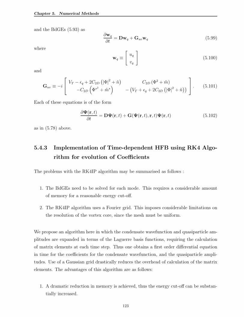
Chapter 5. Numerical Methods
and the BdGEs (5.93) as∂wq
∂t= Dwq + Guvwq (5.99)
where
wq ≡[
uq
vq
]
(5.100)
and
Guv ≡ −i
VT − ǫq + 2C2D
(
|Φ|2 + n)
C2D (Φ2 + m)
−C2D
(
Φ∗2+ m∗
)
−(
VT + ǫq + 2C2D
(
|Φ|2 + n))
. (5.101)
Each of these equations is of the form
∂Ψ(r, t)
∂t= DΨ(r, t) + G(Ψ(r, t), r, t)Ψ(r, t) (5.102)
as in (5.78) above.
5.4.3 Implementation of Time-dependent HFB using RK4 Algo-
rithm for evolution of Coefficients
The problems with the RK4IP algorithm may be summarised as follows :
1. The BdGEs need to be solved for each mode. This requires a considerable amount
of memory for a reasonable energy cut-off.
2. The RK4IP algorithm uses a Fourier grid. This imposes considerable limitations on
the resolution of the vortex core, since the mesh must be uniform.
We propose an algorithm here in which the condensate wavefunction and quasiparticle am-
plitudes are expanded in terms of the Laguerre basis functions, requiring the calculation
of matrix elements at each time step. Thus one obtains a first order differential equation
in time for the coefficients for the condensate wavefunction, and the quasiparticle ampli-
tudes. Use of a Gaussian grid drastically reduces the overhead of calculation of the matrix
elements. The advantages of this algorithm are as follows:
1. A dramatic reduction in memory is achieved, thus the energy cut-off can be substan-
tially increased.
123
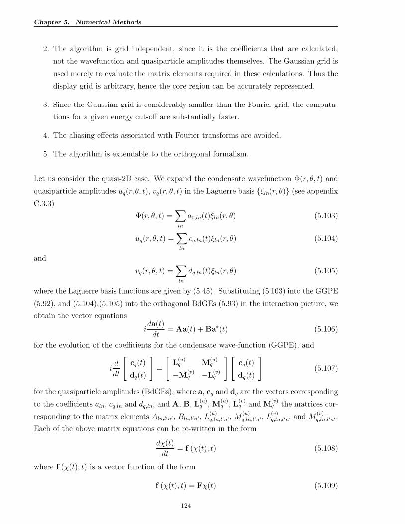
Chapter 5. Numerical Methods
2. The algorithm is grid independent, since it is the coefficients that are calculated,
not the wavefunction and quasiparticle amplitudes themselves. The Gaussian grid is
used merely to evaluate the matrix elements required in these calculations. Thus the
display grid is arbitrary, hence the core region can be accurately represented.
3. Since the Gaussian grid is considerably smaller than the Fourier grid, the computa-
tions for a given energy cut-off are substantially faster.
4. The aliasing effects associated with Fourier transforms are avoided.
5. The algorithm is extendable to the orthogonal formalism.
Let us consider the quasi-2D case. We expand the condensate wavefunction Φ(r, θ, t) and
quasiparticle amplitudes uq(r, θ, t), vq(r, θ, t) in the Laguerre basis ξln(r, θ) (see appendix
C.3.3)
Φ(r, θ, t) =∑
ln
a0,ln(t)ξln(r, θ) (5.103)
uq(r, θ, t) =∑
ln
cq,ln(t)ξln(r, θ) (5.104)
and
vq(r, θ, t) =∑
ln
dq,ln(t)ξln(r, θ) (5.105)
where the Laguerre basis functions are given by (5.45). Substituting (5.103) into the GGPE
(5.92), and (5.104),(5.105) into the orthogonal BdGEs (5.93) in the interaction picture, we
obtain the vector equations
ida(t)
dt= Aa(t) + Ba∗(t) (5.106)
for the evolution of the coefficients for the condensate wave-function (GGPE), and
id
dt
[
cq(t)
dq(t)
]
=
[
L(u)q M
(u)q
−M(v)q −L
(v)q
][
cq(t)
dq(t)
]
(5.107)
for the quasiparticle amplitudes (BdGEs), where a, cq and dq are the vectors corresponding
to the coefficients aln, cq,ln and dq,ln, and A, B, L(u)q , M
(u)q , L
(v)q and M
(v)q the matrices cor-
responding to the matrix elements Aln,l′n′, Bln,l′n′, L(u)q,ln,l′n′, M
(u)q,ln,l′n′, L
(v)q,ln,l′n′ and M
(v)q,ln,l′n′.
Each of the above matrix equations can be re-written in the form
dχ(t)
dt= f (χ(t), t) (5.108)
where f (χ(t), t) is a vector function of the form
f (χ(t), t) = Fχ(t) (5.109)
124
Chapter 5. Numerical Methods
for some matrix F. In the case of the dynamical equation for the evolution of the coefficients
a(t) for the condensate wave-function (GGPE), we can re-write equation (5.106) as
d
dt
[
a(t)
a∗(t)
]
=1
i
[
A B
−B∗ −A∗
][
a(t)
a∗(t)
]
(5.110)
which is of the required form.
We can integrate the vector equation (5.108) using the standard fourth-order Runge-Kutta
algorithm, thus
f (χ(tn+1), tn+1) = f (χ(tn), tn) + [k1 + 2 (k2 + k3) + k4] /6 (5.111)
where
k1 = f (χ(tn), tn) ∆t (5.112)
k2 = f
(
χ(tn +∆t
2) +
k1
2, tn +
∆t
2
)
∆t (5.113)
k3 = f
(
χ(tn +∆t
2) +
k2
2, tn +
∆t
2
)
∆t (5.114)
k4 = f (χ(tn + ∆t) + k3, tn + ∆t) ∆t. (5.115)
Verification of Kohn’s Theorem Preliminary time-independent simulations using both
the RK4IP and the RK4 algorithm for the evolution of the coefficients (not presented here)
verify that Kohn’s theorem is rigorously observed in both cases, as are the number and
angular momentum conservation laws.
Use of Orthogonal Formalism The results obtained using the standard and the or-
thogonal time-dependent HFB formalisms are qualitatively very similar. This was verified
in several simulations, but owing to the extra computational effort required in calculat-
ing the projection part∫
dr′P (r′, r, t)φ(r′, t) in the orthogonal GGPE (5.92) the standard
time-dependent HFB algorithm was used for all of the simulations presented here - see
footnote at the start of section 5.1.
5.5 Gaussian Quadrature
Gaussian quadrature is an integration technique that provides very accurate integration
for a minimal number of grid points. It is applicable to integrands that may be written as
125
Chapter 5. Numerical Methods
the product of a polynomial of order 2N − 1 times a weighting function, i.e. in evaluating
integrals of the form∫ a
b
w(x)P2N−1(x)dx (5.116)
where the P2N−1(x) is a polynomial of order 2N−1 in x and w(x) is a weighting function in
x defined over the closed interval [a, b]. Let fn(x) be a sequence of orthogonal polynomials
of order n in [a, b] relative to the weighting function w(x). Then it can be shown that [91]
∫ a
b
w(x)P2N−1(x)dx =
N∑
k=1
αkP2N−1(xk) (5.117)
where the constants αk are given by
αk =
∫ b
a
w(x)Lk(x)dx (5.118)
with
Lk =
∏
i6=k(x− xi)∏
i6=k(xk − xi)(5.119)
where the xk, k = 1, 2, . . . , N are the zeros of fn(x) = 0.
This shows that the integration is exact for polynomials up to order 2N − 1, given a
sequence fn(x) of orthogonal polynomials. Often the integration accuracy is very good
for polynomials of order greater than 2N−1 provided N is sufficiently large. Well-behaved
functions can also be approximated by the representation w(x)P2N−1(x).
Here the wave-functions and the quasi-particle amplitudes are expanded in the Laguerre
basis, hence defining ρ = r2 and noting that dρ = dr2 = 2rdr, we see that all radial
densities can be written in the form exp(−ρ)P2N+L−2(ρ), and all radial matrix products
in the form exp(−ρ)P4N+2L−4(ρ), so we need 2N + L radial grid points to evaluate radial
matrix densities to machine precision. Regarding the azimuthal coordinate θ, we assume
that the θ-dependence is relatively smooth, and can therefore be well represented by a
polynomial of order 2K − 1 with weighting factor w(x) = 1, and the integrals accurately
evaluated for a grid of K azimuthal grid points using the sequence of Legendre orthogonal
polynomials.
In most of the integrations performed here, Nr = 41 radial points and Nθ = 40 azimuthal
points were used (a grid of 41×40 points), though in certain circumstances involving several
vortices or in cases of vigorous stirring or trap axial symmetry-breaking it was necessary
to use Nr = 61 and Nθ = 60 for accurate integration.
126
Chapter 5. Numerical Methods
5.6 Computational Accuracy and Mode Energy Cut-
off
In view of the large number of calculations necessary, the numbers of computational modes
and grid points were kept to a minimum whilst still maintaining reasonable computational
accuracy (∼ 1−2%). This was verified by doubling the number of computational modes in
certain limited cases, and observing the change. Since the aim here is a proof in principle
of the method of calculation of the precessional frequency and how this correlates with
the LCLS energies, accuracy is not the main concern - only that reasonable accuracy is
maintained, and that the solutions can be refined later, if required. In the calculations here,
209 computational modes were used corresponding to n = 1, . . . , 10 and l = 0,±1, . . . ,±10,
and the effect of doubling the number of computational modes found to be relatively small.
Since Gaussian quadrature (see next section) was used for the radial integration, in most
cases Nr = 41 was sufficient. In some cases involving multiple vortices, this number
was increased to Nr = 61 . Gaussian quadrature was also used for the azimuthal (θ)
integration by use of the Legendre orthogonal polynomials, and provided the change in
angular dependence is not too rapid, Nθ = 40 ensures good computational accuracy. In
some cases involving multiple vortices, this number had to be increased to Nθ = 60.
As we shall see in chapter 7, a mode cut-off of Nm = 100 is sufficient for most vortex pre-
cession calculations. This is not sufficient for the perturbation calculations (not presented
here). In these preliminary calculations, we find that the shifts in the quasi-particle exci-
tation energies have a relatively small effect on the thermal and anomalous densities, and
therefore we would expect the effects on the vortex precession results to be insignificant.
Since the extra computational overhead in the self-consistent calculations for the vortex
precession calculations is significant, the orthogonal time-independent HFB equations are
solved self-consistently with the precessional frequency prediction calculations without the
extra overhead of the self-consistent perturbation calculations.
5.7 Vortex Detection and Tracking Algorithm
5.7.1 Vortex Detection
The vortex detection algorithm is the same as that used by B. M. Caradoc-Davies in his
PhD Thesis [90]. For each point (excluding the grid points on the boundary) a detection
127
Chapter 5. Numerical Methods
grid is set up as shown in figure 5.1 which shows the case of a positive vortex characterised
by a phase-flow in the anti-clockwise direction, and represented by the symbol + indicating
a singly-charged vortex.
Let us define the quantity U(α, β) by [90]
U(α, β) =
−1 if β − α > π
0 if −π ≤ β − α ≤ π
1 if β − α < −π(5.120)
and the set of pairs of wave-function phase angles Aij by
Aij = (φ1, φ2), (φ2, φ3), . . . , (φ7, φ8), (φ8, φ1) (5.121)
where the φi are short-hand representations for the phase-angles
φ1 ≡ arg (Φi−1,j−1)
φ2 ≡ arg (Φi,j−1)
φ3 ≡ arg (Φi+1,j−1)
φ4 ≡ arg (Φi+1,j)
φ5 ≡ arg (Φi+1,j+1)
φ6 ≡ arg (Φi,j+1)
φ7 ≡ arg (Φi−1,j+1)
φ8 ≡ arg (Φi−1,j)
(5.122)
We then define the vortex detection array by [90]
Vij =∑
(α,β)∈Aij
U(α, β). (5.123)
Vij = +1 indicates a vortex of charge +1 at position (i, j) on the grid, and -1 a vortex of
charge -1. The density curvature at point (i, j) is given by [90]
κ =|Φi−1,j|2 + |Φi+1,j |2 − 2 |Φi,j |2
(∆x)2 +|Φi,j−1|2 + |Φi,j+1|2 − 2 |Φi,j|2
(∆y)2. (5.124)
We set up a threshold κν for the detection of vortices, and neglect vortices in low density
regions of the condensate, i.e. for κ < κν . Here we choose κ ∼ 10−1 since we wish only
to track vortices in regions of appreciable density in our stirring and trap axial symmetry-
breaking simulations in order to limit the number of vortex tracks, though this can be
easily changed if necessary.
128
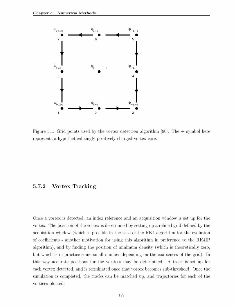
Chapter 5. Numerical Methods
0 1 2 3 4 5 6 7 8
1
2
3
4
5
6
7
1
ψi−1,j−1
8
ψi−1,j
7
ψi−1,j+1
2
ψi,j−1
ψi,j
6
ψi,j+1
3
ψi+1,j−1
4
ψi+1,j
5
ψi+1,j+1
+
Figure 5.1: Grid points used by the vortex detection algorithm [90]. The + symbol here
represents a hypothetical singly positively charged vortex core.
5.7.2 Vortex Tracking
Once a vortex is detected, an index reference and an acquisition window is set up for the
vortex. The position of the vortex is determined by setting up a refined grid defined by the
acquisition window (which is possible in the case of the RK4 algorithm for the evolution
of coefficients - another motivation for using this algorithm in preference to the RK4IP
algorithm), and by finding the position of minimum density (which is theoretically zero,
but which is in practice some small number depending on the coarseness of the grid). In
this way accurate positions for the vortices may be determined. A track is set up for
each vortex detected, and is terminated once that vortex becomes sub-threshold. Once the
simulation is completed, the tracks can be matched up, and trajectories for each of the
vortices plotted.
129
Chapter 5. Numerical Methods
5.8 Presentation of Data where Time Evolution of
HFB Equations is expressed in Coefficients
When using the RK4 algorithm above, one stores only the condensate wavefunction co-
efficients aln(t) and the quasiparticle amplitude coefficients cq,ln(t) and dq,ln(t) for
each time step in a file - ie. the data is not grid dependent. Thus one is free to choose
whatever grid is convenient, over any range desired. Here it is desirable to represent the
data in Cartesian coordinates. The coefficients here are in the Laguerre representation.
From a numerical viewpoint, it is more convenient to use the Hermite representation, since
this is much more efficient numerically, as we will see presently. To do this, one must make
a Laguerre to Hermite transformation of the coefficients. Then any Cartesian grid can be
deployed.
Laguerre-Hermite Transformation To do this one must first create a Hermite-Gaussian
grid in the x- and y- coordinates. Then the condensate wavefunction is given by
Φ(x, y, t) =∑
ln
aln(t)ξln(x, y) (5.125)
where
ξln(x, y) =
(
n!
π (n + |l|)!
)1/2
e−(x2+y2)/2L|l|n
(
x2 + y2)
(x+ isgn (l) y)|l| (5.126)
where L|l|n is a modified Laguerre polynomial of order n, and where
sgn (l) ≡
1 if l ≥ 0
−1 if l < 0.(5.127)
The Hermite basis set is given by ζn(x) where
ζn(x) =
(
1√π2nn!
)1/2
e−x2/2Hn(x) (5.128)
where Hn(x) is a Hermite polynomial of order n. We can express Φ(x, y, t) in terms of
Hermite basis functions by writing
Φ(x, y, t) =∑
mn
bmn(t)ζm(x)ζn(y) (5.129)
We can determine the coefficients bmn(t) in terms of the aln(t) coefficients as follows.
We first note by the orthonormality properties of the Hermite basis functions that
bmn(t) =
∞∫
−∞
∞∫
−∞
dxdyζ∗m(x)ζ∗n(y)Φ(x, y, t) =∑
l′n′
al′n′(t)
∞∫
−∞
∞∫
−∞
dxdyζ∗m(x)ζ∗n(y)ξl′n′(x, y).
(5.130)
130
Chapter 5. Numerical Methods
Thus we can transform from the Laguerre representation into the Hermite representation
using the transformation
bmn(t) =∑
l′n′
al′n′(t)Amn,l′n′ (5.131)
where
Amn,l′n′ ≡∞∫
−∞
∞∫
−∞
dxdyζ∗m(x)ζ∗n(y)ξl′n′(x, y). (5.132)
One can represent this as a matrix transformation
b(t) = Aa(t) (5.133)
by defining the vectors a and b, and the matrix A by
a(t) =
...
a−ln(t)...
aln(t)...
, b(t) =
b00(t)...
bmn(t)...
, A =
· · · A00,−ln · · · A00,ln · · ·...
...
· · · Amn,−ln · · · Amn,ln · · ·...
...
.
(5.134)
Numerically, the Hermite representation is considerably more convenient. Let
χ ≡
ζ0(x0) · · · ζm(x0) · · · ζNm(x0)
......
...
ζ0(xn) · · · ζm(xn) · · · ζNm(xn)
......
...
ζ0(xNx) · · · ζm(xNx
) · · · ζNm(xNx
)
(5.135)
be a matrix of size (Nx×Nm) where Nx represents the number of points in the 1D Cartesian
Gaussian grid, and Nm the number of modes determined by some energy cut-off criterion,
and
B ≡
b00(t) · · · b0n(t) · · · b0Nm(t)
......
...
bm0(t) · · · bmn(t) · · · bmNm(t)
......
...
bNm0(t) · · · bNmn(t) · · · bNmNm(t)
. (5.136)
131
Chapter 5. Numerical Methods
Then the matrix representing the condensate wavefunction Φ(x, y, tn) at time step n defined
by
Φn ≡
Φ(x0, y0, tn) · · · Φ(x0, yj, tn) · · · Φ(x0, yNx, tn)
......
...
Φ(xi, y0, tn) · · · Φ(xi, yj, tn) · · · Φ(xi, yNx, tn)
......
...
Φ(xNx, y0, tn) · · · Φ(xNx
, yj, tn) · · · Φ(xNx, yNx
, tn)
(5.137)
may be computed by pre- and post-multiplication, viz.
Φn = χBχT . (5.138)
One can do the same for the quasiparticle amplitudes using the same transformation, viz.
eq(t) = Acq(t)
fq(t) = Adq(t)(5.139)
where the quasiparticle amplitudes are now given by
uq(x, y, t) =∑
mn
eq,mn(t)ζm(x)ζn(y) (5.140)
and
vq(x, y, t) =∑
mn
fq,mn(t)ζm(x)ζn(y). (5.141)
5.9 Concluding Remarks
In this chapter we presented the numerical algorithms for solving the time-independent
and time-dependent orthogonal HFB equations. It is easy to modify these algorithms
to implement standard HFB calculations. All time-independent calculations in this thesis
were performed using the orthogonal HFB formalism. In the time-dependent case, however,
this implies extra computation and smaller step size to maintain orthogonality to reasonable
accuracy, therefore all the results presented here were performed using standard HFB.
However, many time-dependent simulations have subsequently been repeated using the
orthogonal HFB formalism, but the differences have been insignificant, and therefore have
not been presented here to reduce on bulk of material.
132
Chapter 6. Simulation of Evaporative Cooling of Dilute Quasi-Two Dimensional BECs
Chapter 6
Simulation of Evaporative Cooling of
Dilute Quasi-Two Dimensional BECs
6.1 Introduction
In this chapter, we implement a Gaussian out-coupler, and calculate the g(2) correlation
function for the out-coupled beam. The purpose of this is firstly to test the functionality of
the time-dependent algorithm, and secondly to simulate the cooling of a quasi-2D BEC by
means of evaporative cooling. We perform time-dependent standard HFB calculations to
simulate a cold dilute Bose gas undergoing evaporative cooling. We simulate the adiabatic
cooling process by coupling atoms out of the BEC using a complex coupling potential in
the form of an annulus having a Gaussian cross-sectional profile of starting radius well
outside the Thomas-Fermi radius, and slowly diminishing this radius to a final radius still
lying well outside the Thomas-Fermi radius. Since the thermal atoms lie farthest from
the axis, and there are very few condensate atoms lying outside the Thomas-Fermi radius,
we would expect the out-coupled atoms to be predominantly thermal atoms. This should
provide significant cooling of the condensate. We carry out this procedure for various rates
of cooling, and estimate the effective temperature of the BEC at various times during
the cooling process. We establish the response time of the system, and to what degree
the system equilibrates. However, it should be noted at the outset, that the Landau and
Beliaev processes are missing in the HFB formalism, and therefore we would not expect to
see re-thermalisation. Therefore we would not expect to see any condensate growth, and
any cooling that takes place is due to removal of the high energy particles well outside the
Thomas-Fermi radius.
133
Chapter 6. Simulation of Evaporative Cooling of Dilute Quasi-Two Dimensional BECs
6.2 Coherence Properties of an Out-coupled Beam of
Atoms from a BEC [93,94]
We consider an out-coupling potential −iVc(r, t). This gives us the GGPE
i~∂Φ(r, t)
∂t=(
h(r, t)− iVc(r)− µ+ g(
|Φ(r, t)|2 + 2n(r, t))
)
Φ(r, t) + gm(r, t)Φ∗(r, t)
(6.1)
and the (non-orthogonal) BdGEs
i~ ∂∂t
[
up(r, t)
vp(r, t)
]
=
L(C)(r, t)− ǫq M(r, t)
−M∗(r, t) −(
L(C)∗(r, t) + ǫq
)
[
up(r, t)
vp(r, t)
]
(6.2)
in the interaction-picture, where we have defined the operator L(C)(r, t) by
L(C)(r, t) ≡ L(r, t)− iVc(r, t). (6.3)
Then the rate of change of condensate particles is given by
dNc
dt= −2
~
∫
drVc(r)nc(r) + ig
~
∫
dr(
m(r)Φ∗2
(r)− m∗(r)Φ2(r))
(6.4)
and the rate of change of the thermal population by
dN
dt= −2
~
∫
drVc(r)n(r)− ig~
∫
dr(
m(r)Φ∗2
(r)− m∗(r)Φ2(r))
(6.5)
(see appendix B.2.1), where Nc is the total number of condensate particles and N the total
number of thermal particles. Then if we define Ntot to be the total number of particles in
the BEC, we find that the rate at which particles are coupled out of the BEC is given by
dNtot
dt= −2
~
∫
drVc(r, t)ntot(r, t) (6.6)
where ntot = nc + n. We note that in the absence of the out-coupling potential
dNtot
dt= 0 (6.7)
hence the total number of particles is conserved.
We use the second-order coherence function [92]
g(2)(r, r′, t) =
⟨
ψ†(r, t)ψ†(r′, t)ψ(r′, t)ψ(r, t)⟩
⟨
ψ†(r, t)ψ(r, t)⟩⟨
ψ†(r′, t)ψ(r′, t)⟩ (6.8)
134
Chapter 6. Simulation of Evaporative Cooling of Dilute Quasi-Two Dimensional BECs
and the approximations in [94] to obtain the expression
g(2)(r, r, t) = 2−[
nc(r, t)
nc(r, t) + n(r, t)
]
(6.9)
for the second-order coherence function for the BEC. We approximate the second-order
coherence of the output beam as prescribed in [94] by
g(2)(t) = 2−[
∫
drVc(r, t)nc(r, t)∫
drVc(r, t) (nc(r, t) + n(r, t))
]
. (6.10)
We note that g(2) = 1 indicates a second order coherent gas, whereas g(2) = 2 would indicate
total incoherence (a purely thermal gas). In this way we can quantify the coherence of the
out-coupled beam.
6.3 Simulations for Adiabatic Evaporative Cooling Pro-
cess
We consider here a dilute Bose gas consisting of 2000 87Rb atoms in an axially symmetric
harmonic trap, with radial and axial harmonic trapping frequencies of ωr = 2π×10Hz and
ωz = 2π × 400Hz respectively, having a transition temperature of Tc . 14nK. Thus the
axial confinement is sufficiently strong that all excited axial states may be neglected, hence
the axial (z) component can be integrated out, and the BEC may effectively be treated as
two-dimensional1. We perform time-dependent HFB calculations to simulate a cold dilute
Bose gas initially at T = 12.5nK, undergoing evaporative cooling. In all cases atoms are
coupled out of the BEC using a complex coupling potential in the form of an annulus of
radius ac having a Gaussian cross-sectional profile with amplitude Ac and a full-width at
half maximum (FWHM) of 2√
ln 2sc given by
Vc(r, θ, t) = Ac exp
[
−(
r − aci+ (aci
− acf)t/Tcool
sc
)2]
(6.11)
during the time of cooling, i.e for 0 ≤ t ≤ Tcool, with various amplitudes varying between
0.1~ωr/2 and 200~ωr/2 depending on the duration of cooling Tcool, and with a FWHM
of wFWHM = 4.16r0. The initial radius of the out-coupling potential is aci= 8.5r0 and
is moved in to a final radius of acf= 5.5r0 at a constant rate determined by the time
of cooling Tcool. After the time of cooling, the outcoupling potential is switched off, i.e
1Since Tmax = 12.5nK, the criteria for the two-dimensional approximation are satisfied - see section
5.2.2.
135
Chapter 6. Simulation of Evaporative Cooling of Dilute Quasi-Two Dimensional BECs
Vc(r, θ, t) = 0, for t > Tcool. At the initial radius of 8.5r0 the thermal and condensate
densities, and hence the out-coupled beam are completely negligible. This should simulate
an RF knife used in BEC cooling experiments. However, it should be pointed out that here
we are cooling a BEC, whereas in an experiment a BEC is created by evaporative cooling
of a thermal cloud above the condensation transition temperature. This is due to the limi-
tations of the HFB formalism which is only valid in the presence of a condensate, and does
not predict the growth of a condensate from a thermal cloud. Four cooling simulations
were performed with cooling times of 15 trap cycles, 1 trap cycle, 0.1 trap cycles, and 0.01
trap cycles, thus the behaviour of the BEC can be determined for cooling periods varying
by several orders of magnitude. Since the out-coupling potential always lies outside the
Thomas-Fermi radius, more thermal particles than condensate particles are coupled out of
the condensate, hence the BEC is effectively cooled during this process. This is reflected in
the results shown in figure 6.1 which show the condensate and thermal fractions, and the
g(2) correlation functions2 for each of the simulations, each of the cooling times differing
by an order of magnitude. In all four cases, the condensate function increases substan-
tially, resulting in a cooling of the BEC. At various points during the cooling process, an
effective temperature is estimated by assuming that the process is quasi-static. Hence the
time-independent HFB formalism can be used to determine the effective temperature for
a given thermal density and total number of particles by an iterative process. The effec-
tive temperature is initially estimated using the ideal gas law for a 2D system where the
condensate fraction Fc is given by [107]
Fc = 1− (T/T 2Dc )2 (6.12)
where T 2Dc is the predicted transition temperature for the ideal gas calculated according
to the formula
kBT2Dc = ~
√6ωtrapN
1/2/π. (6.13)
(here T 2Dc ≈ 16.7nK). Thus the thermal fraction can be written as
F = (T/T 2Dc )2. (6.14)
Let Fi be the initial thermal fraction (i.e. prior to cooling) and Ni the initial number of
atoms, and F the thermal fraction and N the number of atoms at the time of the effective
2We see from figures 6.1 I (c), II (c), and III (c) that the g(2) correlation of the out-coupled beam varies
between ∼ 1.8 at the start of the evaporative cooling, diminishing to ∼ 1.4 at the end. This indicates
a predominance of thermal atoms in the out-coupled beam, with the proportion of condensate atoms
increasing as the out-coupling potential moves inwards. As pointed out earlier, the predominance is due
to the fact that the out-coupling potential lies well outside the Thomas-Fermi radius, and this is reflected
in the out-coupled beam being largely incoherent.
136
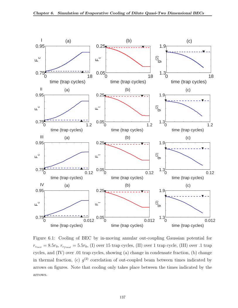
Chapter 6. Simulation of Evaporative Cooling of Dilute Quasi-Two Dimensional BECs
0 180.75
0.95
time (trap cycles)
Fc
I (a)
0 180.05
0.25
time (trap cycles)
Ft
(b)
0 181.3
1.9
time (trap cycles)
g(2)
(c)
0 1.20.75
0.95
time (trap cycles)
Fc
II (a)
0 1.20.05
0.25
time (trap cycles)
Ft
(b)
0 1.21.3
1.9
time (trap cycles)
g(2)
(c)
0 0.120.75
0.95
time (trap cycles)
Fc
III (a)
0 0.120.05
0.25
time (trap cycles)
Ft
(b)
0 0.121.3
1.9
time (trap cycles)
g(2)
(c)
0 0.0120.75
0.95
time (trap cycles)
Fc
IV (a)
0 0.0120.05
0.25
time (trap cycles)
Ft
(b)
0 0.0121.3
1.9
time (trap cycles)
g(2)
(c)
Figure 6.1: Cooling of BEC by in-moving annular out-coupling Gaussian potential for
rcinit= 8.5r0, rcfinal
= 5.5r0, (I) over 15 trap cycles, (II) over 1 trap cycle, (III) over .1 trap
cycles, and (IV) over .01 trap cycles, showing (a) change in condensate fraction, (b) change
in thermal fraction, (c) g(2) correlation of out-coupled beam between times indicated by
arrows on figures. Note that cooling only takes place between the times indicated by the
arrows.
137
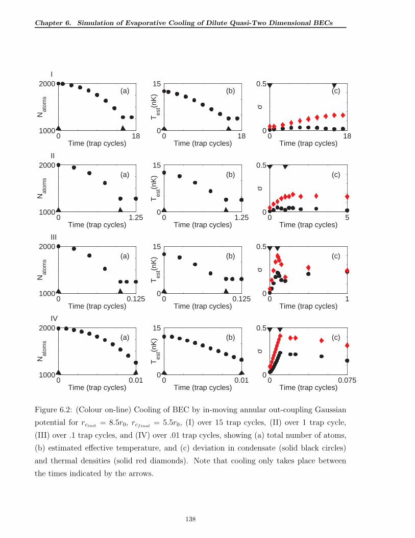
Chapter 6. Simulation of Evaporative Cooling of Dilute Quasi-Two Dimensional BECs
0 181000
2000
Time (trap cycles)
Nat
oms
I
(a)
0 180
15
Time (trap cycles)T
est(n
K) (b)
0 180
0.5
Time (trap cycles)
σ
(c)
0 1.251000
2000
Time (trap cycles)
Nat
oms
II
(a)
0 1.250
15
Time (trap cycles)
Tes
t(nK
) (b)
0 50
0.5
Time (trap cycles)
σ
(c)
0 0.1251000
2000
Time (trap cycles)
Nat
oms
III
(a)
0 0.1250
15
Time (trap cycles)
Tes
t(nK
) (b)
0 10
0.5
Time (trap cycles)
σ(c)
0 0.011000
2000
Time (trap cycles)
Nat
oms
IV
(a)
0 0.010
15
Time (trap cycles)
Tes
t(nK
) (b)
0 0.0750
0.5
Time (trap cycles)
σ
(c)
Figure 6.2: (Colour on-line) Cooling of BEC by in-moving annular out-coupling Gaussian
potential for rcinit= 8.5r0, rcfinal
= 5.5r0, (I) over 15 trap cycles, (II) over 1 trap cycle,
(III) over .1 trap cycles, and (IV) over .01 trap cycles, showing (a) total number of atoms,
(b) estimated effective temperature, and (c) deviation in condensate (solid black circles)
and thermal densities (solid red diamonds). Note that cooling only takes place between
the times indicated by the arrows.
138
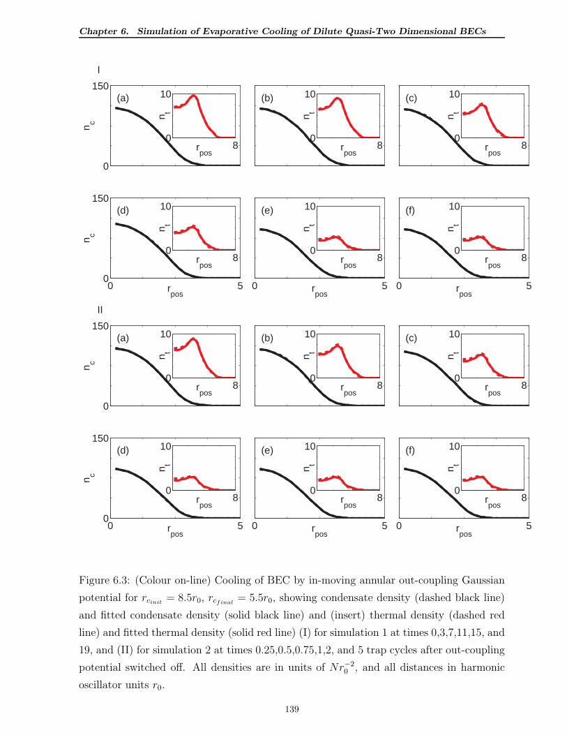
Chapter 6. Simulation of Evaporative Cooling of Dilute Quasi-Two Dimensional BECs
0
150n c
I
(a)
80
10
rpos
n t
(b)
80
10
rpos
n t
(c)
80
10
rpos
n t
0 50
150
rpos
n c
(d)
80
10
rpos
n t
0 5rpos
(e)
80
10
rpos
n t
0 5rpos
(f)
80
10
rpos
n t
0
150
n c
II
(a)
80
10
rpos
n t
(b)
80
10
rpos
n t
(c)
80
10
rpos
n t
0 50
150
rpos
n c
(d)
80
10
rpos
n t
0 5rpos
(e)
80
10
rpos
n t
0 5rpos
(f)
80
10
rpos
n t
Figure 6.3: (Colour on-line) Cooling of BEC by in-moving annular out-coupling Gaussian
potential for rcinit= 8.5r0, rcfinal
= 5.5r0, showing condensate density (dashed black line)
and fitted condensate density (solid black line) and (insert) thermal density (dashed red
line) and fitted thermal density (solid red line) (I) for simulation 1 at times 0,3,7,11,15, and
19, and (II) for simulation 2 at times 0.25,0.5,0.75,1,2, and 5 trap cycles after out-coupling
potential switched off. All densities are in units of Nr−20 , and all distances in harmonic
oscillator units r0.
139
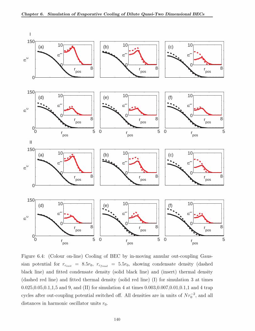
Chapter 6. Simulation of Evaporative Cooling of Dilute Quasi-Two Dimensional BECs
0
150
n c
I
(a)
80
10
rpos
n t
(b)
80
10
rpos
n t
(c)
80
10
rpos
n t
0 50
150
rpos
n c
(d)
80
10
rpos
n t
0 5rpos
(e)
80
10
rpos
n t
0 5rpos
(f)
80
10
rpos
n t
0
150
n c
II
(a)
80
10
rpos
n t
(b)
80
10
rpos
n t
(c)
80
10
rpos
n t
0 50
150
rpos
n c
(d)
80
10
rpos
n t
0 5rpos
(e)
80
10
rpos
n t
0 5rpos
(f)
80
10
rpos
n t
Figure 6.4: (Colour on-line) Cooling of BEC by in-moving annular out-coupling Gaus-
sian potential for rcinit= 8.5r0, rcfinal
= 5.5r0, showing condensate density (dashed
black line) and fitted condensate density (solid black line) and (insert) thermal density
(dashed red line) and fitted thermal density (solid red line) (I) for simulation 3 at times
0.025,0.05,0.1,1,5 and 9, and (II) for simulation 4 at times 0.003,0.007,0.01,0.1,1 and 4 trap
cycles after out-coupling potential switched off. All densities are in units of Nr−20 , and all
distances in harmonic oscillator units r0.
140
Chapter 6. Simulation of Evaporative Cooling of Dilute Quasi-Two Dimensional BECs
temperature estimate. Then the temperature may be estimated from equations (6.13) and
(6.14) according to
Teff ≈
√
N
Ni
Ti (6.15)
where N = NF is the number of thermal particles at the time of the calculation, and
Ni = NiFi is the initial number of thermal particles in the BEC. The time-independent
HFB equations (4.30) and (4.22) are then solved iteratively using this initial estimate for
Teff , given the number of atoms remaining, such that the thermal fraction is the same
as at that time in the cooling experiment. Thus one is able to establish an effective
temperature at any point subject to the assumption of a quasi-static system. Figure 6.2
shows the estimated effective temperature for each of the simulations at various stages
during the cooling process. Also shown in figure 6.2 are the number of atoms left, and
the deviation between the time-dependent and the fitted time-independent condensate
and thermal densities. Here we have defined the deviation σ between the time-dependent
density nTD at time t, and the fitted time-independent density nest
σ(t) ≡√
2
√
∫
dr (nTD(r, t)− nest(r, t))2
∫
dr (nTD(r, t) + nest(r, t))2 . (6.16)
Thus for the condensate the deviation σc would be defined for the densities ncTDand
ncest, and for the thermal population the deviation σt for the densities nTD and nest. In
simulations 1 and 2 the assumption of a quasi-static system is shown to be reasonable in that
the cooling process is on a time-scale that allows for equilibration of the system. However,
there is still a finite deviation due to numerical limitations imposed by the mode cut-off
which drastically reduces the number of accessible states, the fact that we assume a time-
independent quasi-particle basis at the initial temperature, with the initial quasi-particle
spectrum, and the absence of higher order scattering processes in the HFB formalism,
hence the differences in the profiles. We see from figure 6.3 that the forms of the density
profiles are still similar, thus we can reasonably conclude that the assumption of a quasi-
static process is justified in the first two simulations. Simulations 3 and 4, however, are
no longer quasi-static processes since the time-scales of the cooling process do not allow
for equilibration during the cooling process. This is indicated by a sharp increase in
the deviations between the condensate and thermal densities shown in figure 6.2, and the
qualitative differences in the thermal densities as seen in figure 6.4. From these calculations
we can also establish the optimal way to achieve evaporative cooling of a BEC using
an annular out-coupling potential as described above. We see from the above that it is
desirable for the out-coupling to start from as far off-axis as possible - i.e. in regions where
141
Chapter 6. Simulation of Evaporative Cooling of Dilute Quasi-Two Dimensional BECs
there is negligible condensate density (i.e. annular radius ≫ Thomas-Fermi radius), and
to move this in sufficiently slowly so as to maximise the number of thermal atoms and
to minimise the number of condensate atoms coupled out of the BEC. We expect this
to be the case in view of the fact that most of the condensate atoms reside within the
Thomas Fermi radius, whereas we would expect a reasonable proportion of the thermal
atoms to lie outside the Thomas Fermi radius at temperatures 3 T & Tc/2. Here we started
with a condensate at T = 12.5nK (∼ 3Tc/4) with a thermal fraction of ∼ .25. After the
adiabatic cooling, the thermal fraction was ∼ .1, corresponding to an effective temperature
of ∼ 5nK. This is confirmed in our result as shown in figures 6.1 and 6.2 where we see that
the maximum cooling is achieved in simulation 1 for the slowest rate of cooling. However,
simulation 2 is optimal in terms of efficiency of cooling when the time of cooling is also
taken into consideration, and is therefore preferable since this would minimise other losses
such as three-body losses which would become significant over the much longer cooling
times.
We note that there is no evidence of condensate growth in any of our simulations. Sim-
ulations at temperatures much closer to the transition temperature (∼ 0.9Tc), where the
condensate population is very small also show no evidence of condensate growth. This
is due to the fact that significant damping processes (probably the Landau and Beliaev
processes) are not accounted for in HFB due to the quadratic approximation of the Hamil-
tonian, which precludes the terms involving the Landau and Beliaev processes. Hence there
is no equilibration of the system within the time-scales of the experiment, and there is no
condensate growth, as one would have anticipated. Hence, whilst we do observe cooling of
the BEC, we don’t observe evaporative cooling leading to the growth of a condensate as
we would in an experiment.
3Here Tc is the transition temperature of the BEC, and is somewhat lower than the ideal gas predicted
transition temperature of T 2Dc ≈ 16.7nK. We estimate that Tc . 14nK.
142
Chapter 7. Vortices in Quasi-Two Dimensional BECs
Chapter 7
Vortices in Quasi-Two Dimensional
BECs
7.1 Introduction
Quantised vortices are perhaps the single most striking manifestation of superfluidity. Of
particular interest here are the dynamics of vortices in Bose Einstein condensates (BECs).
In 1999, Matthews et. al. [96] used an off-axis resonant laser in order to provide a rotating
gradient in the AC Stark shift across the condensate. The definitive experiment was
conducted by Madison et. al. [97] (see also [98]) towards the end of 1999, in which a
focused laser beam was used to stir a BEC of 87Rb confined in a magnetic trap. Various
methods have been used to create and detect vortices, see, for example, [42, 85, 99–102].
Much of the earlier theoretical work on the dynamics of vortices (see, for example, [36–38,
79]) assumed zero temperature, and neglected the effects of the non-condensate dynamics
on the overall dynamics of the vortex. The Bogoliubov spectrum has a lowest-lying energy
that is negative, the so-called anomalous mode [39,40,82]. The lowest-lying energy is zero
in the frame rotating at this frequency, leading one to conclude that this is the precessional
frequency of the vortex [39, 40, 82].
Solving the Hartree-Fock-Bogoliubov (HFB) equations for an on-axis vortex at finite tem-
perature in the Popov approximation in a regime having sufficiently strong interactions
yields a positive lowest lying energy mode, referred to as the lowest core localised state
(LCLS) [2, 3]. This was then generalised to a lower bound for the LCLS energy for an
off-axis vortex [86]. In both cases it is argued that the thermal cloud acts as an effective
143
Chapter 7. Vortices in Quasi-Two Dimensional BECs
potential, thereby stabilising the vortex, but this fails to take into account the dynamics of
the thermal cloud itself. The association of this energy with the precessional frequency of
the vortex [2,3] leads to the conclusion that the vortex precesses in the direction opposite
to the condensate flow around the core. This is inconsistent with experiment and also
seems intuitively unreasonable, since zero temperature predictions would suggest other-
wise [39, 40, 82] and one might reasonably expect continuous variation with temperature.
Later finite temperature calculations for off-axis vortices by Isoshima et. al. [4], however,
conclude that no correlation exists between the precessional frequency and the anomalous
mode.
To resolve this anomaly, we provide a full solution to the HFB equations for an off-axis
vortex, making a novel use of the continuity equation for the condensate density to establish
the vortex precessional frequency. Our model consists of a dilute Bose gas consisting of
2000 87Rb atoms in an axially symmetric harmonic trap, with radial and axial harmonic
trapping frequencies of ωr = 2π × 10Hz and ωz = 2π × 400Hz respectively, having a
transition temperature of Tc . 14nK. Thus the axial confinement is sufficiently strong
that all excited axial states may be neglected1, so the BEC may effectively be treated as
two-dimensional, but not strong enough to affect the scattering, which is still essentially
three-dimensional. Thus the BEC may be treated as two-dimensional from a computational
viewpoint, since the axial dependency may be integrated out.
7.2 Time-Independent, Axially Symmetric Solutions
In view of the above argument, we restrict ourselves to two-dimensions, and use the di-
mensionless units in section (5.2.2). The 2D time-independent HFB equations in the di-
mensionless units used here are given by the GGPE (5.36) and the BdGEs (5.37).
Before commencing with our calculations for off-axis vortices and the predictions for their
precessional frequencies, we perform time-independent on-axis vortex calculations in the
Popov approximation as a comparison with the results of [2, 3]. We make use of the axial
symmetry of the condensate and quasi-particle wave-functions, obtaining a set of radial
GGPEs and BdGEs for the case of a single on-axis vortex.
Let us consider a ground state having an on-axis vortex of vorticity m (m = 0 corre-
1Here Tmax = 7.5nK, and therefore the criteria for the quasi-two-dimensional approximation are satis-
fied (see section 5.2.2).
144
Chapter 7. Vortices in Quasi-Two Dimensional BECs
sponds to a ground state having no vortices). The general expression for the condensate
wavefunction expanded in the Laguerre basis is given by
Φ(r, θ) =∑
l,n
alnξln(r, θ) (7.1)
where the Laguerre basis function ξln(r, θ) is given by (see appendix C.1.5)
ξln(r, θ) =eilθ
√2πξln(r) (7.2)
with
ξln(r) = N |l|n e
−r2/2r|l|L|l|n (r2) (7.3)
and where L|l|n (r2) is an associated Laguerre polynomial. The Laguerre basis function
ξln(r, θ) satisfies the single-particle eigenvalue equation (as can be verified by substituting
(C.26) into (5.35), and by applying (5.44))
hΩ(r, θ)ξln(r, θ) =(
µ(SP )ln − lΩ
)
ξln(r, θ) (7.4)
where we have defined (c.f. (5.35))
hΩ(r, θ) = −(
∂2
∂r2+
1
r
∂
∂r+
1
r2
∂2
∂θ2
)
+ iΩ∂
∂θ+ r2, (7.5)
hence the motivation in using the Laguerre basis. In view of the axial symmetry of the
solutions, we can write
Φ(r, θ) =eimθ
√2π
Φ(r) (7.6)
where
Φ(r) =∑
n
anξmn(r) (7.7)
where m is the vorticity of the on-axis vortex. Here the aln, l 6= m are considered to be
zero since we are considering a vortex of vorticity m, and we use the short-hand notation
an ≡ amn. Clearly the condensate density nc(r, θ) can be written as
nc(r, θ) =1
2πnc(r) (7.8)
We can also write the quasiparticle amplitudes uq(r, θ) and vq(r, θ) in the form
ulq(r, θ) =ei(l+m)θ
√2π
ulq(r) (7.9)
vlq(r, θ) =ei(l−m)θ
√2π
vlq(r) (7.10)
145
Chapter 7. Vortices in Quasi-Two Dimensional BECs
whereulq(r) =
∑
n cq,lnξl+m,n(r)
vlq(r) =∑
n dq,lnξl−m,n(r).(7.11)
Hence the thermal and anomalous densities n(r, θ) and m(r, θ) can be written as
n(r, θ) =1
2πn(r) (7.12)
and
m(r, θ) =e2imθ
2πm(r) (7.13)
respectively. So, multiplying by e−imθ/√
2π for the GGPE (5.36), and by e−i(l+m)θ/√
2π
and e−i(l−m)θ/√
2π for the first and second of the BdGEs (5.37), and integrating over all θ,
we obtain the time-independent radial HFB equations, where the radial time-independent
GGPE is given by (5.47) (note the radial wave-function is real, i.e. Φ∗(r) = Φ(r))
∆µΦ(r) =(
hm(r)− µ+ CR2D
(
|Φ(r)|2 + 2n(r))
)
Φ(r)+CR2Dm(r)Φ(r)−
∫ ∞
0
r′dr′P (r′, r)φ(r′)
(7.14)
and the radial BdGEs by (5.48)
ǫlq
[
ulq(r)
vlq(r)
]
=∫∞
0r′dr′
[
Ql(r, r′)Ll+m(r′) Ql(r, r
′)M(r′)
−Ql(r, r′)M(r′) −Ql(r, r
′)L−(l−m)(r′)
][
ulq(r′)
vlq(r′)
]
(7.15)
Here we have defined the radial operators Ll(r) andM(r) by (5.49)
Ll(r) ≡ hl(r)− µ+ 2CR2D
(
|Φ(r)|2 + n(r))
M(r) ≡ CR2D (Φ2(r) + m(r))
(7.16)
and the operator P (r′, r) by (5.50)
P (r′, r) ≡(
n(r′, r)L(r′) + m(r′, r)M∗(r′))
/√
Nc(t) (7.17)
with hl(r) given by (5.51)
hl(r) ≡ −(
d2
dr2+
1
r
d
dr
)
+l2
r2− µ+ r2. (7.18)
The radial projection operator Q(r, r′) is given by (5.53)
Ql(r, r′) = δ(r − r′)− δl,0φ(r)φ(r′) (7.19)
The radial 2D nonlinearity constant CR2D ≡ C2D/2π is given by (5.54)
CR2D = 4
(
λ
2π
)1/2as
r0N. (7.20)
146
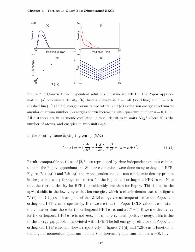
Chapter 7. Vortices in Quasi-Two Dimensional BECs
0 100
120
Position in Trap
Den
sity
(a)
0 100
60
Position in Trap
Den
sity
(b)
0 50
0.1(c)
T (nK)
LCLS
ene
rgy
−10 100
20
l
ε n,l
(d)
Figure 7.1: On-axis time-independent solutions for standard HFB in the Popov approxi-
mation, (a) condensate density, (b) thermal density at T = 1nK (solid line) and T = 5nK
(dashed line), (c) LCLS energy versus temperature, and (d) excitation energy spectrum vs
angular quantum number l - energies shown increasing with quantum number n = 0, 1, . . ..
All distances are in harmonic oscillator units r0, densities in units Nr−20 where N is the
number of atoms, and energies in trap units ~ωr.
In the rotating frame hl,Ω(r) is given by (5.52)
hl,Ω(r) ≡ −(
d2
dr2+
1
r
d
dr
)
+l2
r2− lΩ− µ+ r2. (7.21)
Results comparable to those of [2, 3] are reproduced by time-independent on-axis calcula-
tions in the Popov approximation. Similar calculations were done using orthogonal HFB.
Figures 7.1(a),(b) and 7.2(a),(b) show the condensate and non-condensate density profiles
in the plane passing through the vortex for the Popov and orthogonal HFB cases. Note
that the thermal density for HFB is considerably less than for Popov. This is due to the
upward shift in the low-lying excitation energies, which is clearly demonstrated in figures
7.1(c) and 7.2(c) which are plots of the LCLS energy versus temperature for the Popov and
orthogonal HFB cases respectively. Here we see that the Popov LCLS values are substan-
tially smaller than those for the orthogonal HFB case, and at T = 0nK we see that ǫLCLS
for the orthogonal HFB case is not zero, but some very small positive energy. This is due
to the energy gap problem associated with HFB. The full energy spectra for the Popov and
orthogonal HFB cases are shown respectively in figures 7.1(d) and 7.2(d) as a function of
the angular momentum quantum number l for increasing quantum number n = 0, 1, . . ..
147
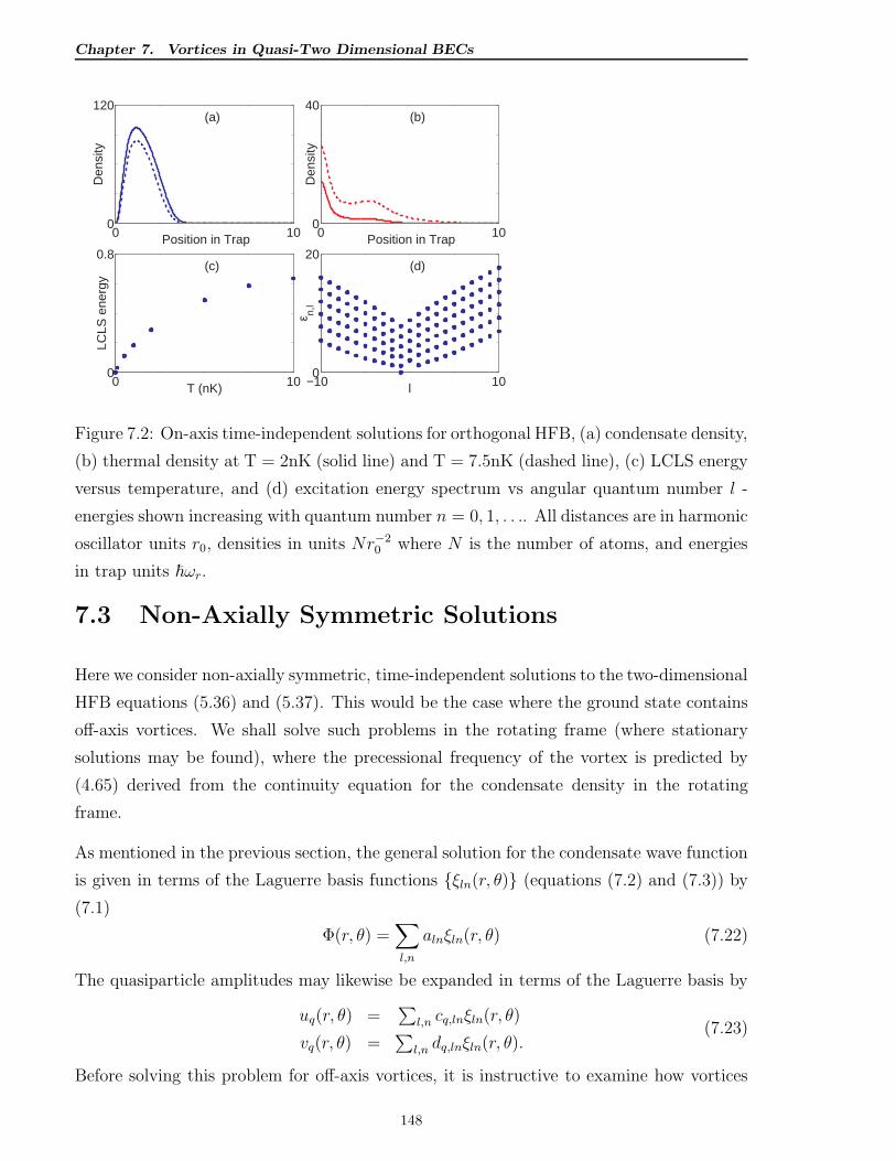
Chapter 7. Vortices in Quasi-Two Dimensional BECs
0 100
120
Position in Trap
Den
sity
(a)
0 100
40
Position in Trap
Den
sity
(b)
0 100
0.8(c)
T (nK)
LCLS
ene
rgy
−10 100
20
l
ε n,l
(d)
Figure 7.2: On-axis time-independent solutions for orthogonal HFB, (a) condensate density,
(b) thermal density at T = 2nK (solid line) and T = 7.5nK (dashed line), (c) LCLS energy
versus temperature, and (d) excitation energy spectrum vs angular quantum number l -
energies shown increasing with quantum number n = 0, 1, . . .. All distances are in harmonic
oscillator units r0, densities in units Nr−20 where N is the number of atoms, and energies
in trap units ~ωr.
7.3 Non-Axially Symmetric Solutions
Here we consider non-axially symmetric, time-independent solutions to the two-dimensional
HFB equations (5.36) and (5.37). This would be the case where the ground state contains
off-axis vortices. We shall solve such problems in the rotating frame (where stationary
solutions may be found), where the precessional frequency of the vortex is predicted by
(4.65) derived from the continuity equation for the condensate density in the rotating
frame.
As mentioned in the previous section, the general solution for the condensate wave function
is given in terms of the Laguerre basis functions ξln(r, θ) (equations (7.2) and (7.3)) by
(7.1)
Φ(r, θ) =∑
l,n
alnξln(r, θ) (7.22)
The quasiparticle amplitudes may likewise be expanded in terms of the Laguerre basis by
uq(r, θ) =∑
l,n cq,lnξln(r, θ)
vq(r, θ) =∑
l,n dq,lnξln(r, θ).(7.23)
Before solving this problem for off-axis vortices, it is instructive to examine how vortices
148
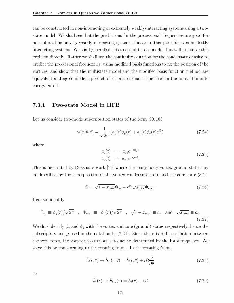
Chapter 7. Vortices in Quasi-Two Dimensional BECs
can be constructed in non-interacting or extremely weakly-interacting systems using a two-
state model. We shall see that the predictions for the precessional frequencies are good for
non-interacting or very weakly interacting systems, but are rather poor for even modestly
interacting systems. We shall generalise this to a multi-state model, but will not solve this
problem directly. Rather we shall use the continuity equation for the condensate density to
predict the precessional frequencies, using modified basis functions to fix the position of the
vortices, and show that the multistate model and the modified basis function method are
equivalent and agree in their prediction of precessional frequencies in the limit of infinite
energy cutoff.
7.3.1 Two-state Model in HFB
Let us consider two-mode superposition states of the form [90,105]
Φ(r, θ, t) =1√2π
(
ag(t)φg(r) + av(t)φv(r)eiθ)
(7.24)
where
ag(t) = ag0e−iµgt
av(t) = av0e−iµvt.
(7.25)
This is motivated by Rokshar’s work [79] where the many-body vortex ground state may
be described by the superposition of the vortex condensate state and the core state (3.1)
Φ =√
1− xcoreΦm + eiχ√xcoreΦcore. (7.26)
Here we identify
Φm ≡ φg(r)/√
2π , Φcore ≡ φv(r)/√
2π ,√
1− xcore ≡ ag and√xcore ≡ av.
(7.27)
We thus identify φv and φg with the vortex and core (ground) states respectively, hence the
subscripts v and g used in the notation in (7.24). Since there is Rabi oscillation between
the two states, the vortex precesses at a frequency determined by the Rabi frequency. We
solve this by transforming to the rotating frame. In the rotating frame
h(r, θ)→ hΩ(r, θ) = h(r, θ) + iΩ∂
∂θ(7.28)
so
hl(r)→ hΩ,l(r) = hl(r)− Ωl (7.29)
149
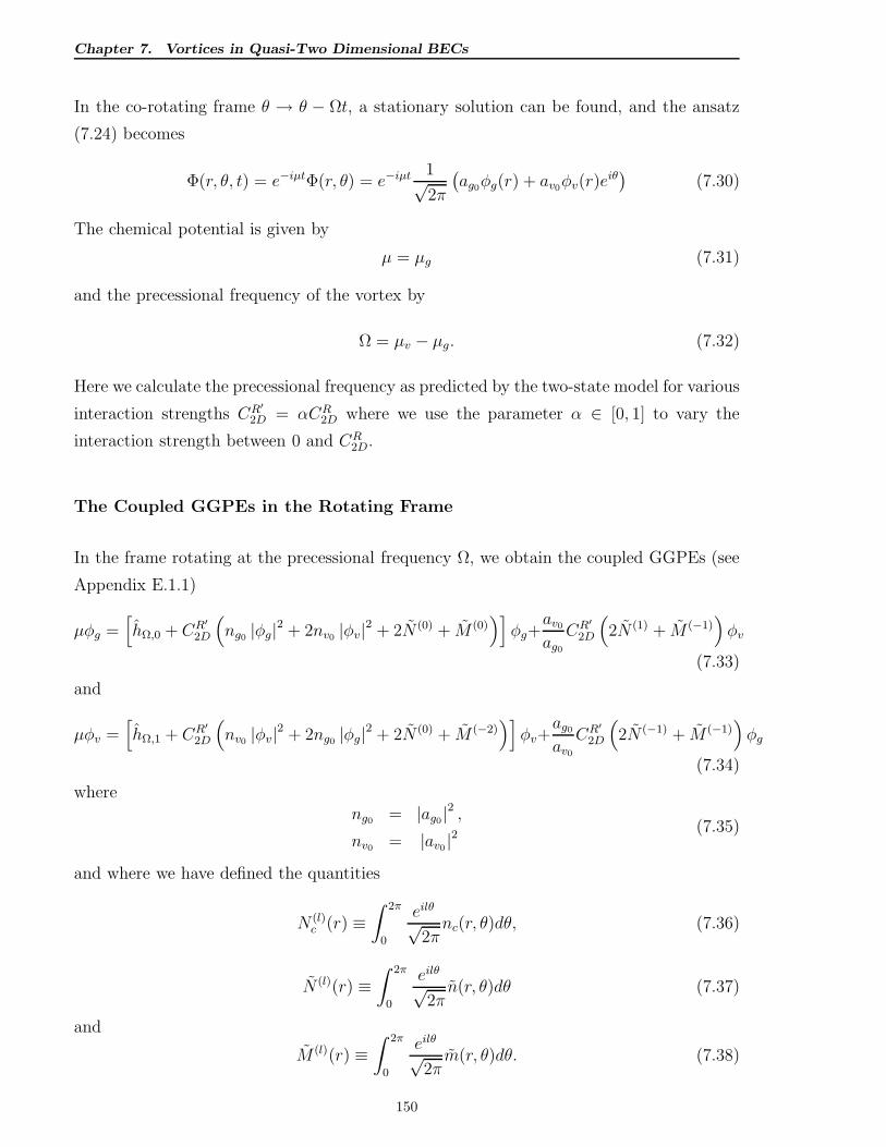
Chapter 7. Vortices in Quasi-Two Dimensional BECs
In the co-rotating frame θ → θ − Ωt, a stationary solution can be found, and the ansatz
(7.24) becomes
Φ(r, θ, t) = e−iµtΦ(r, θ) = e−iµt 1√2π
(
ag0φg(r) + av0φv(r)eiθ)
(7.30)
The chemical potential is given by
µ = µg (7.31)
and the precessional frequency of the vortex by
Ω = µv − µg. (7.32)
Here we calculate the precessional frequency as predicted by the two-state model for various
interaction strengths CR′
2D = αCR2D where we use the parameter α ∈ [0, 1] to vary the
interaction strength between 0 and CR2D.
The Coupled GGPEs in the Rotating Frame
In the frame rotating at the precessional frequency Ω, we obtain the coupled GGPEs (see
Appendix E.1.1)
µφg =[
hΩ,0 + CR′
2D
(
ng0 |φg|2 + 2nv0 |φv|2 + 2N (0) + M (0))]
φg+av0
ag0
CR′
2D
(
2N (1) + M (−1))
φv
(7.33)
and
µφv =[
hΩ,1 + CR′
2D
(
nv0 |φv|2 + 2ng0 |φg|2 + 2N (0) + M (−2))]
φv+ag0
av0
CR′
2D
(
2N (−1) + M (−1))
φg
(7.34)
where
ng0 = |ag0|2 ,nv0 = |av0 |2
(7.35)
and where we have defined the quantities
N (l)c (r) ≡
∫ 2π
0
eilθ
√2πnc(r, θ)dθ, (7.36)
N (l)(r) ≡∫ 2π
0
eilθ
√2πn(r, θ)dθ (7.37)
and
M (l)(r) ≡∫ 2π
0
eilθ
√2πm(r, θ)dθ. (7.38)
150
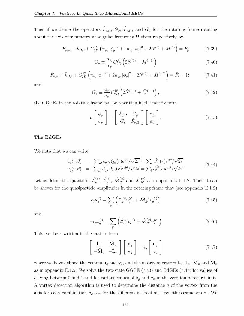
Chapter 7. Vortices in Quasi-Two Dimensional BECs
Then if we define the operators Fg,Ω, Gg, Fv,Ω, and Gv for the rotating frame rotating
about the axis of symmetry at angular frequency Ω given respectively by
Fg,Ω ≡ hΩ,0 + CR′
2D
(
ng0 |φg|2 + 2nv0 |φv|2 + 2N (0) + M (0))
= Fg (7.39)
Gg ≡av0
ag0
CR′
2D
(
2N (1) + M (−1))
(7.40)
Fv,Ω ≡ hΩ,1 + CR′
2D
(
nv0 |φv|2 + 2ng0 |φg|2 + 2N (0) + M (−2))
= Fv − Ω (7.41)
and
Gv ≡ag0
av0
CR′
2D
(
2N (−1) + M (−1))
, (7.42)
the GGPEs in the rotating frame can be rewritten in the matrix form
µ
[
φg
φv
]
=
[
Fg,Ω Gg
Gv Fv,Ω
][
φg
φv
]
. (7.43)
The BdGEs
We note that we can write
uq(r, θ) =∑
nl cq,lnξln(r)eilθ/√
2π =∑
l u(l)q (r)eilθ/
√2π
vq(r, θ) =∑
nl dq,lnξln(r)eilθ/√
2π =∑
l v(l)q (r)eilθ/
√2π.
(7.44)
Let us define the quantities L(u)ll′ , L(v)
ll′ , M(u)ll′ and M(v)
ll′ as in appendix E.1.2. Then it can
be shown for the quasiparticle amplitudes in the rotating frame that (see appendix E.1.2)
ǫqu(l)q =
∑
l′
(
L(u)ll′ u
(l′)q + M(u)
ll′ v(l′)q
)
(7.45)
and
−ǫqv(l)q =
∑
l′
(
L(v)ll′ v
(l′)q + M(v)
ll′ u(l′)q
)
(7.46)
This can be rewritten in the matrix form[
Lu Mu
−Mv −Lv
][
uq
vq
]
= ǫq
[
uq
vq
]
(7.47)
where we have defined the vectors uq and vq, and the matrix operators Lu, Lv, Mu and Mv
as in appendix E.1.2. We solve the two-state GGPE (7.43) and BdGEs (7.47) for values of
α lying between 0 and 1 and for various values of ag and av in the zero temperature limit.
A vortex detection algorithm is used to determine the distance a of the vortex from the
axis for each combination aa, av for the different interaction strength parameters α. We
151
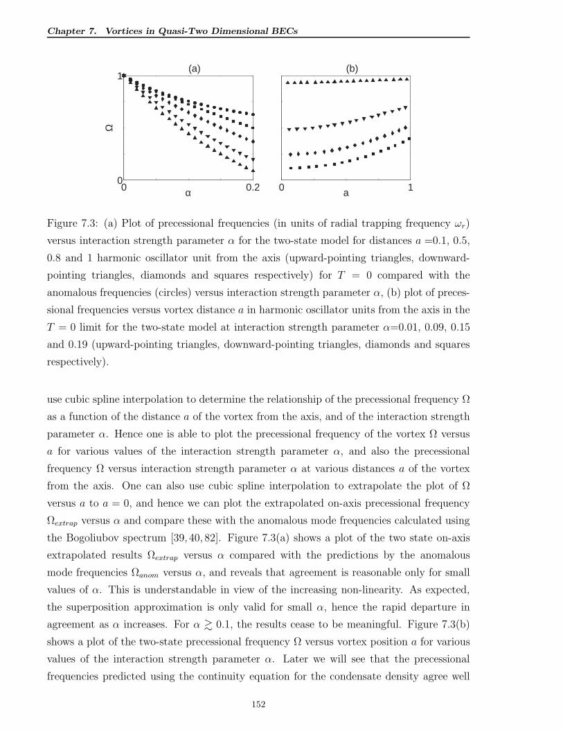
Chapter 7. Vortices in Quasi-Two Dimensional BECs
0 0.20
1(a)
α
Ω
0 1
(b)
a
Figure 7.3: (a) Plot of precessional frequencies (in units of radial trapping frequency ωr)
versus interaction strength parameter α for the two-state model for distances a =0.1, 0.5,
0.8 and 1 harmonic oscillator unit from the axis (upward-pointing triangles, downward-
pointing triangles, diamonds and squares respectively) for T = 0 compared with the
anomalous frequencies (circles) versus interaction strength parameter α, (b) plot of preces-
sional frequencies versus vortex distance a in harmonic oscillator units from the axis in the
T = 0 limit for the two-state model at interaction strength parameter α=0.01, 0.09, 0.15
and 0.19 (upward-pointing triangles, downward-pointing triangles, diamonds and squares
respectively).
use cubic spline interpolation to determine the relationship of the precessional frequency Ω
as a function of the distance a of the vortex from the axis, and of the interaction strength
parameter α. Hence one is able to plot the precessional frequency of the vortex Ω versus
a for various values of the interaction strength parameter α, and also the precessional
frequency Ω versus interaction strength parameter α at various distances a of the vortex
from the axis. One can also use cubic spline interpolation to extrapolate the plot of Ω
versus a to a = 0, and hence we can plot the extrapolated on-axis precessional frequency
Ωextrap versus α and compare these with the anomalous mode frequencies calculated using
the Bogoliubov spectrum [39, 40, 82]. Figure 7.3(a) shows a plot of the two state on-axis
extrapolated results Ωextrap versus α compared with the predictions by the anomalous
mode frequencies Ωanom versus α, and reveals that agreement is reasonable only for small
values of α. This is understandable in view of the increasing non-linearity. As expected,
the superposition approximation is only valid for small α, hence the rapid departure in
agreement as α increases. For α & 0.1, the results cease to be meaningful. Figure 7.3(b)
shows a plot of the two-state precessional frequency Ω versus vortex position a for various
values of the interaction strength parameter α. Later we will see that the precessional
frequencies predicted using the continuity equation for the condensate density agree well
152
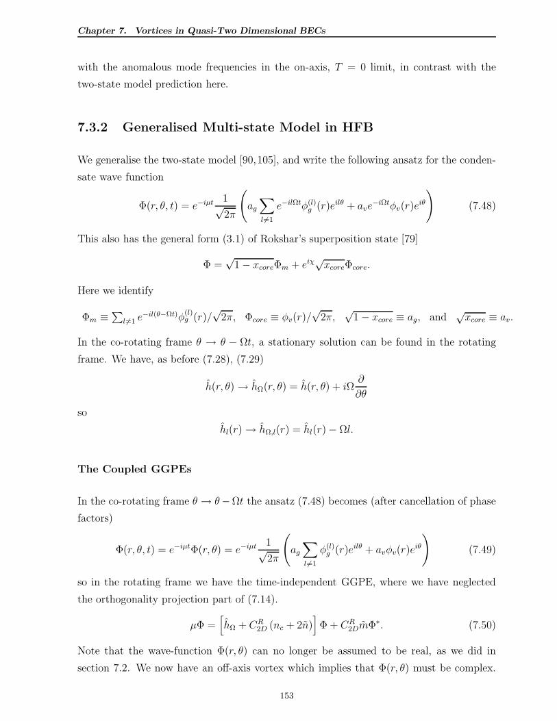
Chapter 7. Vortices in Quasi-Two Dimensional BECs
with the anomalous mode frequencies in the on-axis, T = 0 limit, in contrast with the
two-state model prediction here.
7.3.2 Generalised Multi-state Model in HFB
We generalise the two-state model [90,105], and write the following ansatz for the conden-
sate wave function
Φ(r, θ, t) = e−iµt 1√2π
(
ag
∑
l 6=1
e−ilΩtφ(l)g (r)eilθ + ave
−iΩtφv(r)eiθ
)
(7.48)
This also has the general form (3.1) of Rokshar’s superposition state [79]
Φ =√
1− xcoreΦm + eiχ√xcoreΦcore.
Here we identify
Φm ≡∑
l 6=1 e−il(θ−Ωt)φ
(l)g (r)/
√2π, Φcore ≡ φv(r)/
√2π,
√1− xcore ≡ ag, and
√xcore ≡ av.
In the co-rotating frame θ → θ − Ωt, a stationary solution can be found in the rotating
frame. We have, as before (7.28), (7.29)
h(r, θ)→ hΩ(r, θ) = h(r, θ) + iΩ∂
∂θ
so
hl(r)→ hΩ,l(r) = hl(r)− Ωl.
The Coupled GGPEs
In the co-rotating frame θ → θ−Ωt the ansatz (7.48) becomes (after cancellation of phase
factors)
Φ(r, θ, t) = e−iµtΦ(r, θ) = e−iµt 1√2π
(
ag
∑
l 6=1
φ(l)g (r)eilθ + avφv(r)e
iθ
)
(7.49)
so in the rotating frame we have the time-independent GGPE, where we have neglected
the orthogonality projection part of (7.14).
µΦ =[
hΩ + CR2D (nc + 2n)
]
Φ + CR2DmΦ∗. (7.50)
Note that the wave-function Φ(r, θ) can no longer be assumed to be real, as we did in
section 7.2. We now have an off-axis vortex which implies that Φ(r, θ) must be complex.
153
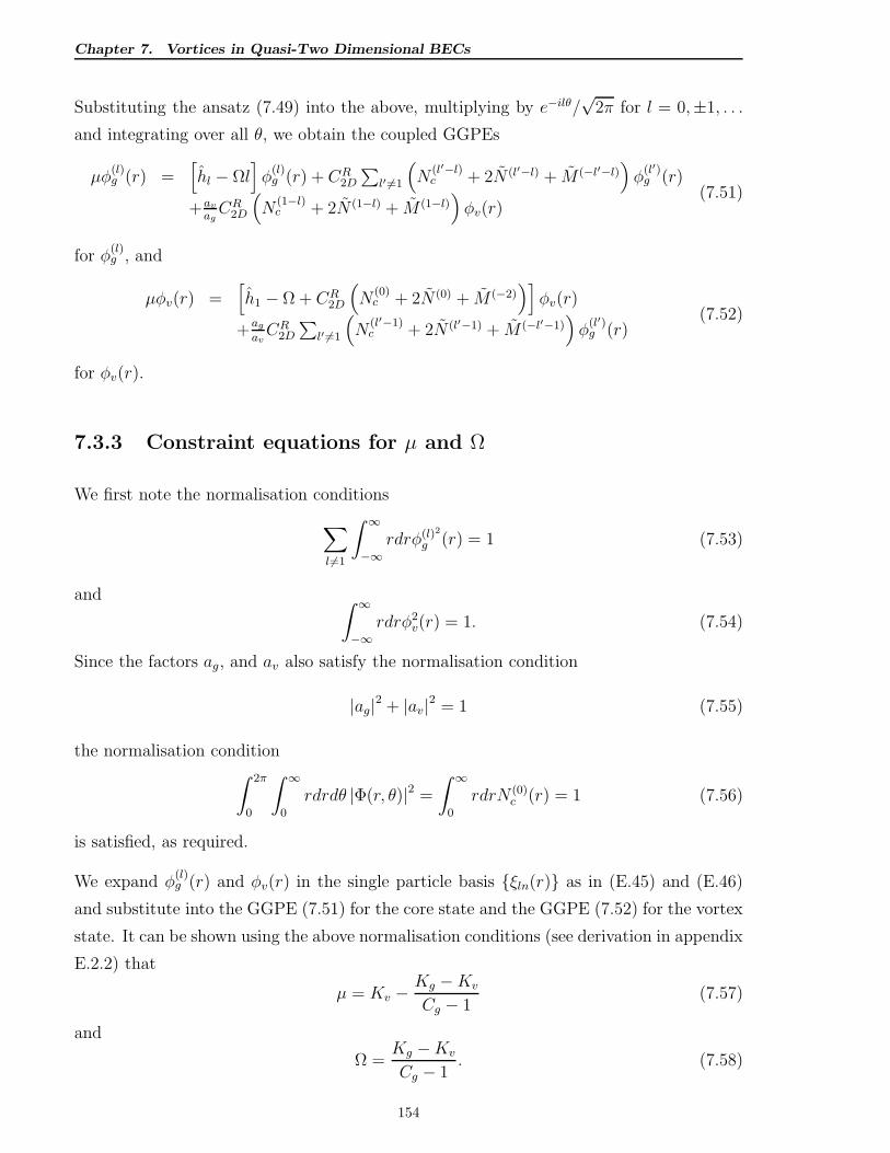
Chapter 7. Vortices in Quasi-Two Dimensional BECs
Substituting the ansatz (7.49) into the above, multiplying by e−ilθ/√
2π for l = 0,±1, . . .
and integrating over all θ, we obtain the coupled GGPEs
µφ(l)g (r) =
[
hl − Ωl]
φ(l)g (r) + CR
2D
∑
l′ 6=1
(
N(l′−l)c + 2N (l′−l) + M (−l′−l)
)
φ(l′)g (r)
+av
agCR
2D
(
N(1−l)c + 2N (1−l) + M (1−l)
)
φv(r)(7.51)
for φ(l)g , and
µφv(r) =[
h1 − Ω + CR2D
(
N(0)c + 2N (0) + M (−2)
)]
φv(r)
+ag
avCR
2D
∑
l′ 6=1
(
N(l′−1)c + 2N (l′−1) + M (−l′−1)
)
φ(l′)g (r)
(7.52)
for φv(r).
7.3.3 Constraint equations for µ and Ω
We first note the normalisation conditions
∑
l 6=1
∫ ∞
−∞rdrφ(l)2
g (r) = 1 (7.53)
and∫ ∞
−∞rdrφ2
v(r) = 1. (7.54)
Since the factors ag, and av also satisfy the normalisation condition
|ag|2 + |av|2 = 1 (7.55)
the normalisation condition∫ 2π
0
∫ ∞
0
rdrdθ |Φ(r, θ)|2 =
∫ ∞
0
rdrN (0)c (r) = 1 (7.56)
is satisfied, as required.
We expand φ(l)g (r) and φv(r) in the single particle basis ξln(r) as in (E.45) and (E.46)
and substitute into the GGPE (7.51) for the core state and the GGPE (7.52) for the vortex
state. It can be shown using the above normalisation conditions (see derivation in appendix
E.2.2) that
µ = Kv −Kg −Kv
Cg − 1(7.57)
and
Ω =Kg −Kv
Cg − 1. (7.58)
154
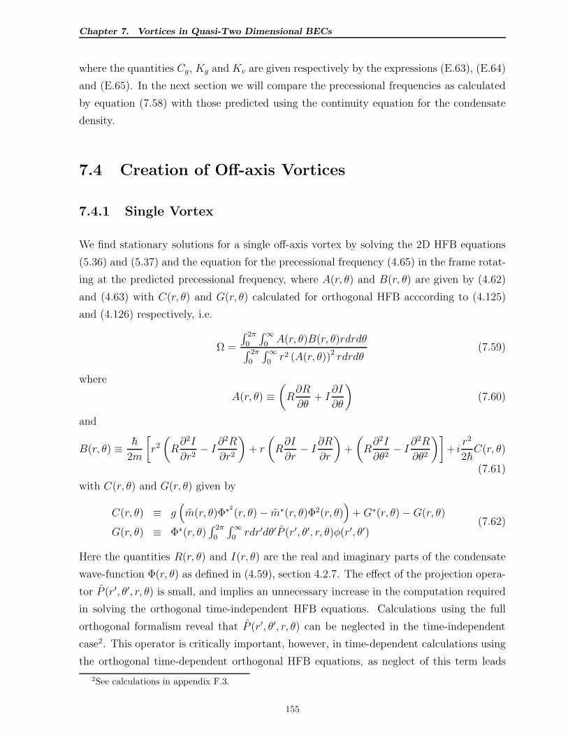
Chapter 7. Vortices in Quasi-Two Dimensional BECs
where the quantities Cg, Kg and Kv are given respectively by the expressions (E.63), (E.64)
and (E.65). In the next section we will compare the precessional frequencies as calculated
by equation (7.58) with those predicted using the continuity equation for the condensate
density.
7.4 Creation of Off-axis Vortices
7.4.1 Single Vortex
We find stationary solutions for a single off-axis vortex by solving the 2D HFB equations
(5.36) and (5.37) and the equation for the precessional frequency (4.65) in the frame rotat-
ing at the predicted precessional frequency, where A(r, θ) and B(r, θ) are given by (4.62)
and (4.63) with C(r, θ) and G(r, θ) calculated for orthogonal HFB acccording to (4.125)
and (4.126) respectively, i.e.
Ω =
∫ 2π
0
∫∞0A(r, θ)B(r, θ)rdrdθ
∫ 2π
0
∫∞0r2 (A(r, θ))2 rdrdθ
(7.59)
where
A(r, θ) ≡(
R∂R
∂θ+ I
∂I
∂θ
)
(7.60)
and
B(r, θ) ≡ ~
2m
[
r2
(
R∂2I
∂r2− I ∂
2R
∂r2
)
+ r
(
R∂I
∂r− I ∂R
∂r
)
+
(
R∂2I
∂θ2− I ∂
2R
∂θ2
)]
+ ir2
2~C(r, θ)
(7.61)
with C(r, θ) and G(r, θ) given by
C(r, θ) ≡ g(
m(r, θ)Φ∗2(r, θ)− m∗(r, θ)Φ2(r, θ)
)
+G∗(r, θ)−G(r, θ)
G(r, θ) ≡ Φ∗(r, θ)∫ 2π
0
∫∞0rdr′dθ′P (r′, θ′, r, θ)φ(r′, θ′)
(7.62)
Here the quantities R(r, θ) and I(r, θ) are the real and imaginary parts of the condensate
wave-function Φ(r, θ) as defined in (4.59), section 4.2.7. The effect of the projection opera-
tor P (r′, θ′, r, θ) is small, and implies an unnecessary increase in the computation required
in solving the orthogonal time-independent HFB equations. Calculations using the full
orthogonal formalism reveal that P (r′, θ′, r, θ) can be neglected in the time-independent
case2. This operator is critically important, however, in time-dependent calculations using
the orthogonal time-dependent orthogonal HFB equations, as neglect of this term leads
2See calculations in appendix F.3.
155
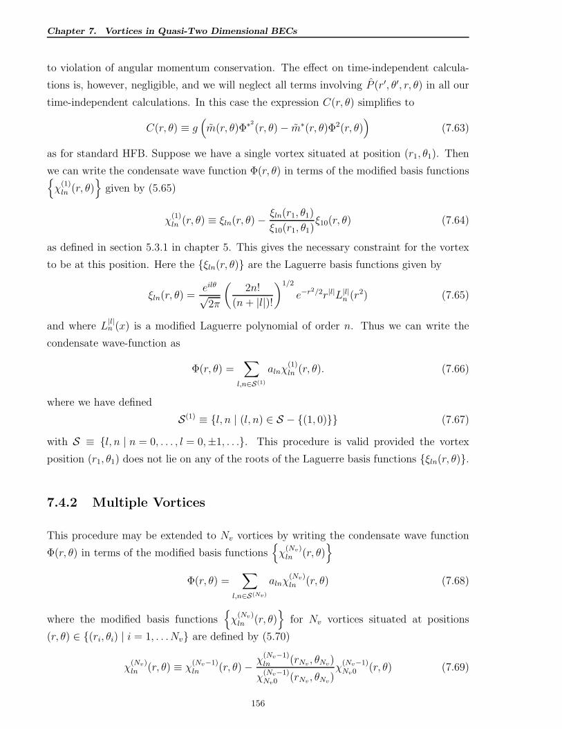
Chapter 7. Vortices in Quasi-Two Dimensional BECs
to violation of angular momentum conservation. The effect on time-independent calcula-
tions is, however, negligible, and we will neglect all terms involving P (r′, θ′, r, θ) in all our
time-independent calculations. In this case the expression C(r, θ) simplifies to
C(r, θ) ≡ g(
m(r, θ)Φ∗2
(r, θ)− m∗(r, θ)Φ2(r, θ))
(7.63)
as for standard HFB. Suppose we have a single vortex situated at position (r1, θ1). Then
we can write the condensate wave function Φ(r, θ) in terms of the modified basis functions
χ(1)ln (r, θ)
given by (5.65)
χ(1)ln (r, θ) ≡ ξln(r, θ)− ξln(r1, θ1)
ξ10(r1, θ1)ξ10(r, θ) (7.64)
as defined in section 5.3.1 in chapter 5. This gives the necessary constraint for the vortex
to be at this position. Here the ξln(r, θ) are the Laguerre basis functions given by
ξln(r, θ) =eilθ
√2π
(
2n!
(n + |l|)!
)1/2
e−r2/2r|l|L|l|n (r2) (7.65)
and where L|l|n (x) is a modified Laguerre polynomial of order n. Thus we can write the
condensate wave-function as
Φ(r, θ) =∑
l,n∈S(1)
alnχ(1)ln (r, θ). (7.66)
where we have defined
S(1) ≡ l, n | (l, n) ∈ S − (1, 0) (7.67)
with S ≡ l, n | n = 0, . . . , l = 0,±1, . . .. This procedure is valid provided the vortex
position (r1, θ1) does not lie on any of the roots of the Laguerre basis functions ξln(r, θ).
7.4.2 Multiple Vortices
This procedure may be extended to Nv vortices by writing the condensate wave function
Φ(r, θ) in terms of the modified basis functions
χ(Nv)ln (r, θ)
Φ(r, θ) =∑
l,n∈S(Nv)
alnχ(Nv)ln (r, θ) (7.68)
where the modified basis functions
χ(Nv)ln (r, θ)
for Nv vortices situated at positions
(r, θ) ∈ (ri, θi) | i = 1, . . .Nv are defined by (5.70)
χ(Nv)ln (r, θ) ≡ χ
(Nv−1)ln (r, θ)− χ
(Nv−1)ln (rNv
, θNv)
χ(Nv−1)Nv0 (rNv
, θNv)χ
(Nv−1)Nv0 (r, θ) (7.69)
156
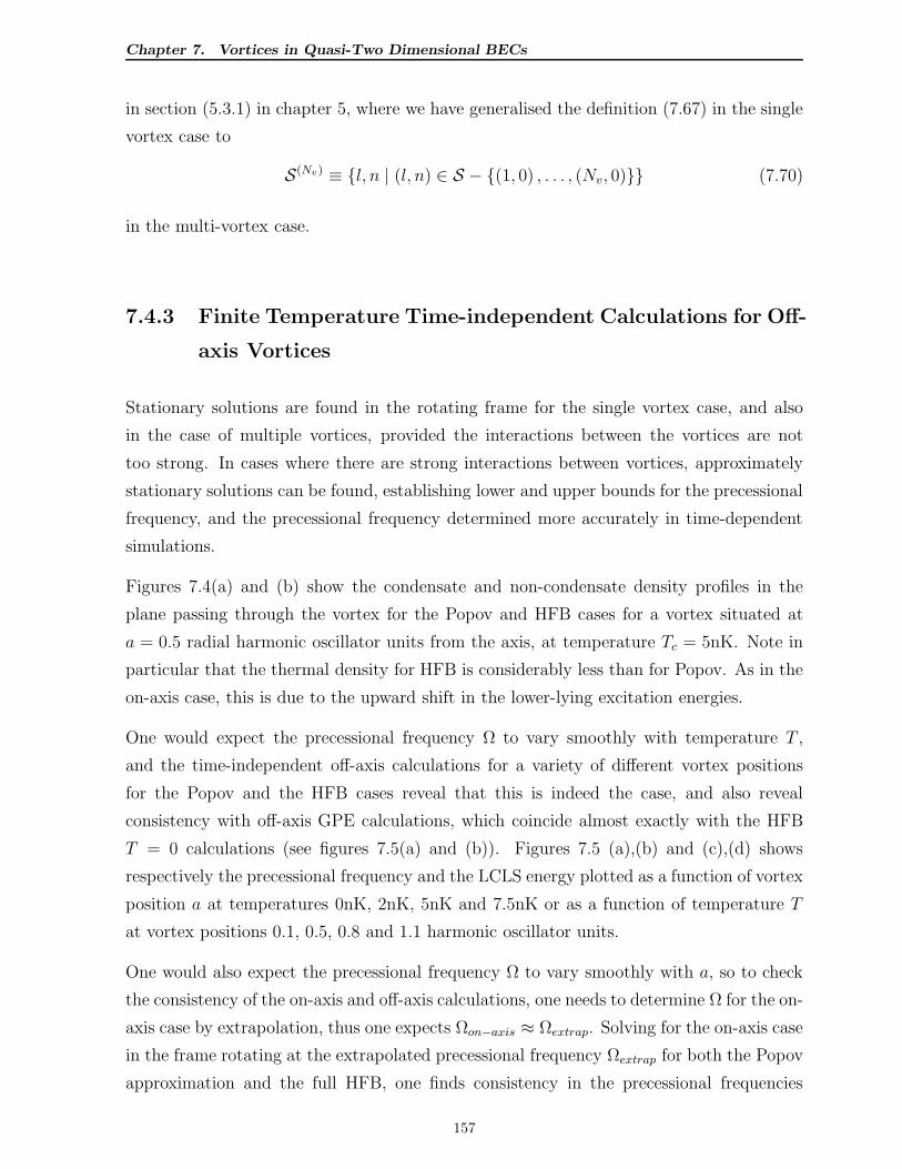
Chapter 7. Vortices in Quasi-Two Dimensional BECs
in section (5.3.1) in chapter 5, where we have generalised the definition (7.67) in the single
vortex case to
S(Nv) ≡ l, n | (l, n) ∈ S − (1, 0) , . . . , (Nv, 0) (7.70)
in the multi-vortex case.
7.4.3 Finite Temperature Time-independent Calculations for Off-
axis Vortices
Stationary solutions are found in the rotating frame for the single vortex case, and also
in the case of multiple vortices, provided the interactions between the vortices are not
too strong. In cases where there are strong interactions between vortices, approximately
stationary solutions can be found, establishing lower and upper bounds for the precessional
frequency, and the precessional frequency determined more accurately in time-dependent
simulations.
Figures 7.4(a) and (b) show the condensate and non-condensate density profiles in the
plane passing through the vortex for the Popov and HFB cases for a vortex situated at
a = 0.5 radial harmonic oscillator units from the axis, at temperature Tc = 5nK. Note in
particular that the thermal density for HFB is considerably less than for Popov. As in the
on-axis case, this is due to the upward shift in the lower-lying excitation energies.
One would expect the precessional frequency Ω to vary smoothly with temperature T ,
and the time-independent off-axis calculations for a variety of different vortex positions
for the Popov and the HFB cases reveal that this is indeed the case, and also reveal
consistency with off-axis GPE calculations, which coincide almost exactly with the HFB
T = 0 calculations (see figures 7.5(a) and (b)). Figures 7.5 (a),(b) and (c),(d) shows
respectively the precessional frequency and the LCLS energy plotted as a function of vortex
position a at temperatures 0nK, 2nK, 5nK and 7.5nK or as a function of temperature T
at vortex positions 0.1, 0.5, 0.8 and 1.1 harmonic oscillator units.
One would also expect the precessional frequency Ω to vary smoothly with a, so to check
the consistency of the on-axis and off-axis calculations, one needs to determine Ω for the on-
axis case by extrapolation, thus one expects Ωon−axis ≈ Ωextrap. Solving for the on-axis case
in the frame rotating at the extrapolated precessional frequency Ωextrap for both the Popov
approximation and the full HFB, one finds consistency in the precessional frequencies
157
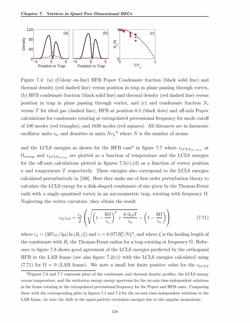
Chapter 7. Vortices in Quasi-Two Dimensional BECs
−5 0 50
40
80
120
Position in Trap
Den
sity
(a)
−5 0 5Position in Trap
(b)
0 10
1
T/Tc
Nc/N
(c)
Figure 7.4: (a) (Colour on-line) HFB Popov Condensate fraction (black solid line) and
thermal density (red dashed line) versus position in trap in plane passing through vortex,
(b) HFB condensate fraction (black solid line) and thermal density (red dashed line) versus
position in trap in plane passing through vortex, and (c) and condensate fraction Nc
versus T for ideal gas (dashed line), HFB at position 0.5 (black dots) and off-axis Popov
calculations for condensate rotating at extrapolated precessional frequency for mode cutoff
of 100 modes (red triangles), and 1639 modes (red squares). All distances are in harmonic
oscillator units r0, and densities in units Nr−20 where N is the number of atoms.
and the LCLS energies as shown for the HFB case3 in figure 7.7 where ǫLCLSon−axisat
Ωextrap and ǫLCLSextrapare plotted as a function of temperature and the LCLS energies
for the off-axis calculations plotted in figures 7.5(c),(d) as a function of vortex position
a and temperature T respectively. These energies also correspond to the LCLS energies
calculated perturbatively in [106]. Here they make use of first order perturbation theory to
calculate the LCLS energy for a disk-shaped condensate of size given by the Thomas-Fermi
radii with a singly-quantised vortex in an axi-symmetric trap, rotating with frequency Ω.
Neglecting the vortex curvature, they obtain the result
ǫLCLS =ǫa2
√
(
1− ~Ω
ǫa
)2
+4γkBT
ǫa−(
1− ~Ω
ǫa
)
(7.71)
where ǫa = (3~2ωr/4µ) ln (Rr/ξ) and γ = 0.077R2r/Nξ
4, and where ξ is the healing length of
the condensate with Rr the Thomas-Fermi radius for a trap rotating at frequency Ω. Refer-
ence to figure 7.8 shows good agreement of the LCLS energies predicted by the orthogonal
HFB in the LAB frame (see also figure 7.2(c)) with the LCLS energies calculated using
(7.71) for Ω = 0 (LAB frame). We note a small but finite positive value for the ǫLCLS
3Figures 7.6 and 7.7 represent plots of the condensate and thermal density profiles, the LCLS energy
versus temperature, and the excitation energy energy spectrum for the on-axis time-independent solutions
in the frame rotating at the extrapolated precessional frequency for the Popov and HFB cases. Comparing
these with the corresponding plots in figures 7.1 and 7.2 for the on-axis time-independent solutions in the
LAB frame, we note the shift in the quasi-particle excitation energies due to the angular momentum.
158
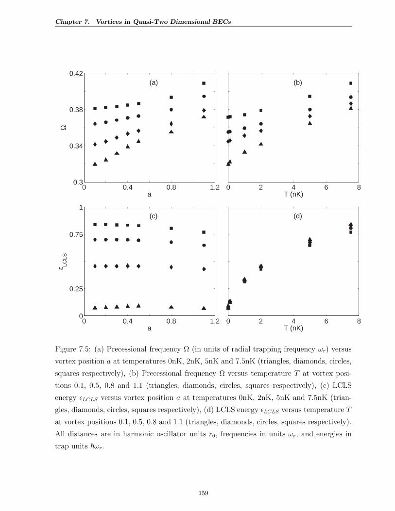
Chapter 7. Vortices in Quasi-Two Dimensional BECs
0 0.4 0.8 1.20.3
0.34
0.38
0.42
a
Ω
(a)
0 2 4 6 8T (nK)
(b)
0 0.4 0.8 1.20
0.25
0.75
1
a
ε LCLS
(c)
0 2 4 6 8T (nK)
(d)
Figure 7.5: (a) Precessional frequency Ω (in units of radial trapping frequency ωr) versus
vortex position a at temperatures 0nK, 2nK, 5nK and 7.5nK (triangles, diamonds, circles,
squares respectively), (b) Precessional frequency Ω versus temperature T at vortex posi-
tions 0.1, 0.5, 0.8 and 1.1 (triangles, diamonds, circles, squares respectively), (c) LCLS
energy ǫLCLS versus vortex position a at temperatures 0nK, 2nK, 5nK and 7.5nK (trian-
gles, diamonds, circles, squares respectively), (d) LCLS energy ǫLCLS versus temperature T
at vortex positions 0.1, 0.5, 0.8 and 1.1 (triangles, diamonds, circles, squares respectively).
All distances are in harmonic oscillator units r0, frequencies in units ωr, and energies in
trap units ~ωr.
159
Chapter 7. Vortices in Quasi-Two Dimensional BECs
calculation using orthogonal HFB corresponding to the energy gap in the HFB energy
spectrum and the quantum depletion.
We note from figure 7.5 that there is absolutely no correlation between the precessional
frequencies and the LCLS energies, contrary to the claims of [2, 3]. The excitation due
to ǫLCLS is given by the mode density corresponding to the LCLS mode, and has nothing
to do with precession. The precessional frequencies are determined by the conservation of
flow (the continuity equation for the condensate density), and hence by equation (7.59).
These calculations also predict precession in the same sense as the circulation, as one would
expect, contrary to [2, 3].
We note further that ǫLCLS varies continuously with T , and we see that ǫLCLS|T≈0 is always
some small value. Due to quantum depletion ǫLCLS > 0 always, even at T = 0 for HFB
and HFB (Popov).
We also find consistency in the condensate fractions between the on-axis and off-axis cal-
culations, and Figure 7.4(c) shows a plot of the condensate fraction Nc versus T (nK) for
the off-axis case for HFB, and the on-axis case for Popov for a mode cutoff of 100. Addi-
tional points are shown for Popov for mode cutoff4 of 1639. Shown also is Nc versus T for
the ideal gas calculations with Tc ≈ 16.7nK. The predicted transition temperature Tc is
calculated according to the calculation [107]
kBT2Dc = ~
√6ωtrapN
1/2/π (7.72)
for a radially harmonically trapped 2D Bose gas. The condensate fraction dependence on
T is given by
Fc = 1− (T/T 2Dc )2. (7.73)
The results reveal that the mode cutoff of 100 is sufficient for T . 7.5nK, but the results
for T & Tc/2 become unreliable. At these temperatures, the HFB formalism is unreliable
anyway [108], so a cutoff of 100 modes represents an adequate computational investment.
At this cutoff, for T ≈ 5nK, one estimates an error of ∼ 10% in thermal population
which does not qualitatively affect our results. We also perform off-axis calculations for
triangular and hexagonal vortex arrays. Plots of Ω versus temperature T at various values
4The mode cut-off Ncut is limited by the number of computational modes as follows: Suppose the
quantum numbers n and l are limited to n = 1, . . . , N and l = 0,±1, . . . ,±M , then the number of
computational modes for the BdGEs is given by Ncomp = N(2M + 1) − 1, and clearly the mode cut-off
cannot exceed the number of computational modes, i.e. Ncut ≤ Ncomp. In most of the computations
done here, N = 10 and M = 10, so Ncomp = 209, and we have chosen Ncomp = 100 to optimise the
computational investment. The case of Ncut = 1639 corresponds to N = 40 and M = 20.
160
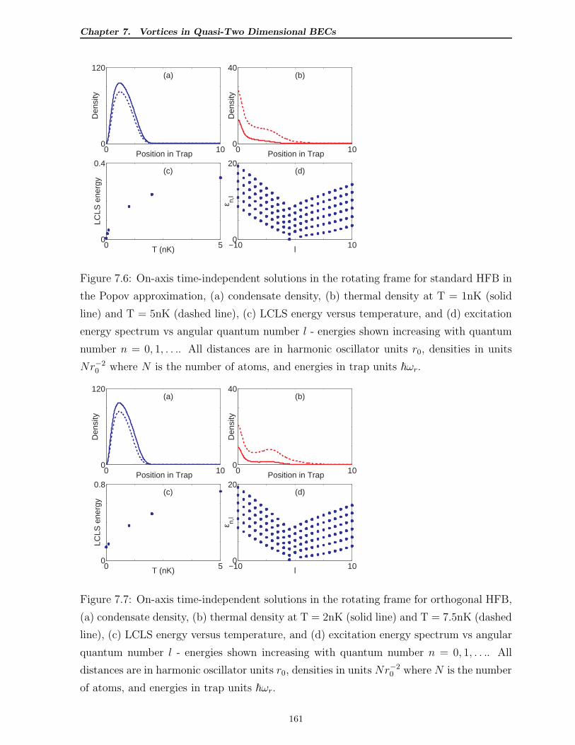
Chapter 7. Vortices in Quasi-Two Dimensional BECs
0 100
120
Position in Trap
Den
sity
(a)
0 100
40
Position in Trap
Den
sity
(b)
0 50
0.4(c)
T (nK)
LCLS
ene
rgy
−10 100
20
l
ε n,l
(d)
Figure 7.6: On-axis time-independent solutions in the rotating frame for standard HFB in
the Popov approximation, (a) condensate density, (b) thermal density at T = 1nK (solid
line) and T = 5nK (dashed line), (c) LCLS energy versus temperature, and (d) excitation
energy spectrum vs angular quantum number l - energies shown increasing with quantum
number n = 0, 1, . . .. All distances are in harmonic oscillator units r0, densities in units
Nr−20 where N is the number of atoms, and energies in trap units ~ωr.
0 100
120
Position in Trap
Den
sity
(a)
0 100
40
Position in Trap
Den
sity
(b)
0 50
0.8(c)
T (nK)
LCLS
ene
rgy
−10 100
20
l
ε n,l
(d)
Figure 7.7: On-axis time-independent solutions in the rotating frame for orthogonal HFB,
(a) condensate density, (b) thermal density at T = 2nK (solid line) and T = 7.5nK (dashed
line), (c) LCLS energy versus temperature, and (d) excitation energy spectrum vs angular
quantum number l - energies shown increasing with quantum number n = 0, 1, . . .. All
distances are in harmonic oscillator units r0, densities in units Nr−20 where N is the number
of atoms, and energies in trap units ~ωr.
161
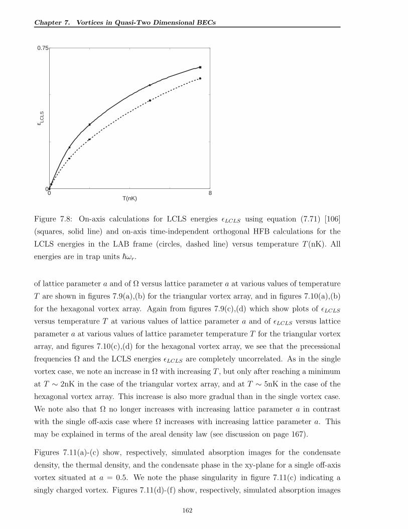
Chapter 7. Vortices in Quasi-Two Dimensional BECs
0 80
0.75
T(nK)
ε LCLS
Figure 7.8: On-axis calculations for LCLS energies ǫLCLS using equation (7.71) [106]
(squares, solid line) and on-axis time-independent orthogonal HFB calculations for the
LCLS energies in the LAB frame (circles, dashed line) versus temperature T (nK). All
energies are in trap units ~ωr.
of lattice parameter a and of Ω versus lattice parameter a at various values of temperature
T are shown in figures 7.9(a),(b) for the triangular vortex array, and in figures 7.10(a),(b)
for the hexagonal vortex array. Again from figures 7.9(c),(d) which show plots of ǫLCLS
versus temperature T at various values of lattice parameter a and of ǫLCLS versus lattice
parameter a at various values of lattice parameter temperature T for the triangular vortex
array, and figures 7.10(c),(d) for the hexagonal vortex array, we see that the precessional
frequencies Ω and the LCLS energies ǫLCLS are completely uncorrelated. As in the single
vortex case, we note an increase in Ω with increasing T , but only after reaching a minimum
at T ∼ 2nK in the case of the triangular vortex array, and at T ∼ 5nK in the case of the
hexagonal vortex array. This increase is also more gradual than in the single vortex case.
We note also that Ω no longer increases with increasing lattice parameter a in contrast
with the single off-axis case where Ω increases with increasing lattice parameter a. This
may be explained in terms of the areal density law (see discussion on page 167).
Figures 7.11(a)-(c) show, respectively, simulated absorption images for the condensate
density, the thermal density, and the condensate phase in the xy-plane for a single off-axis
vortex situated at a = 0.5. We note the phase singularity in figure 7.11(c) indicating a
singly charged vortex. Figures 7.11(d)-(f) show, respectively, simulated absorption images
162
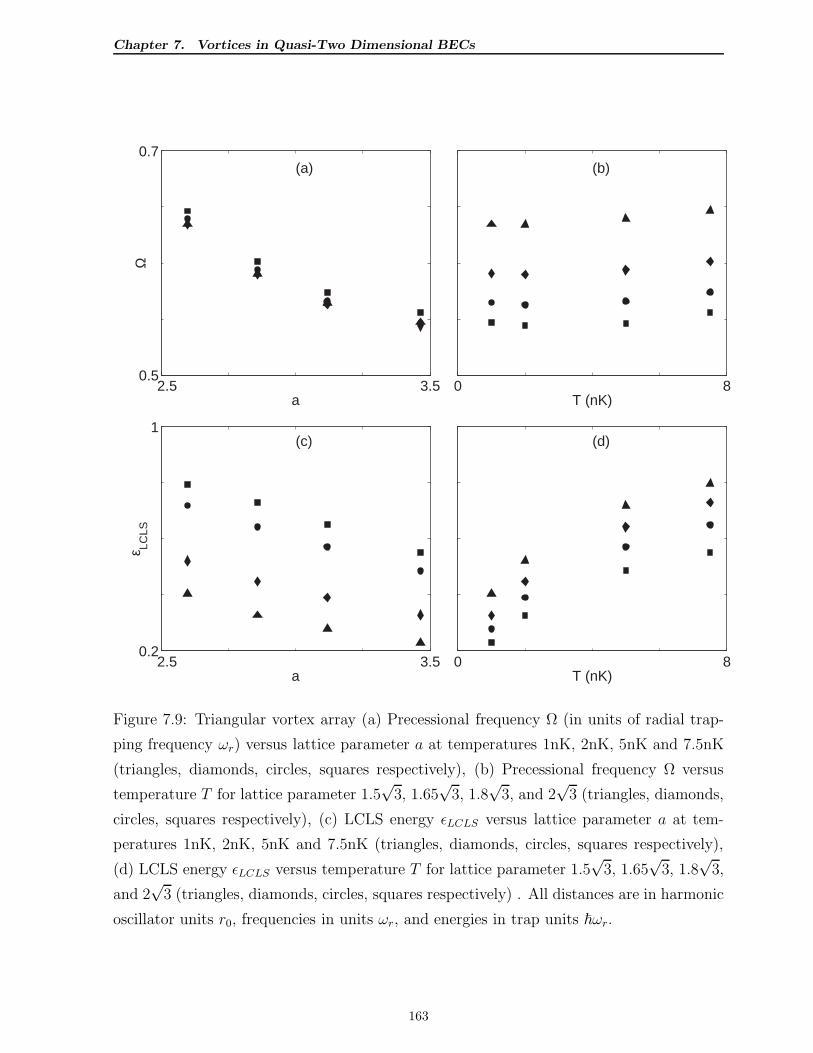
Chapter 7. Vortices in Quasi-Two Dimensional BECs
2.5 3.50.5
0.7
a
Ω
(a)
0 8T (nK)
(b)
2.5 3.50.2
1
a
ε LCLS
(c)
0 8T (nK)
(d)
Figure 7.9: Triangular vortex array (a) Precessional frequency Ω (in units of radial trap-
ping frequency ωr) versus lattice parameter a at temperatures 1nK, 2nK, 5nK and 7.5nK
(triangles, diamonds, circles, squares respectively), (b) Precessional frequency Ω versus
temperature T for lattice parameter 1.5√
3, 1.65√
3, 1.8√
3, and 2√
3 (triangles, diamonds,
circles, squares respectively), (c) LCLS energy ǫLCLS versus lattice parameter a at tem-
peratures 1nK, 2nK, 5nK and 7.5nK (triangles, diamonds, circles, squares respectively),
(d) LCLS energy ǫLCLS versus temperature T for lattice parameter 1.5√
3, 1.65√
3, 1.8√
3,
and 2√
3 (triangles, diamonds, circles, squares respectively) . All distances are in harmonic
oscillator units r0, frequencies in units ωr, and energies in trap units ~ωr.
163
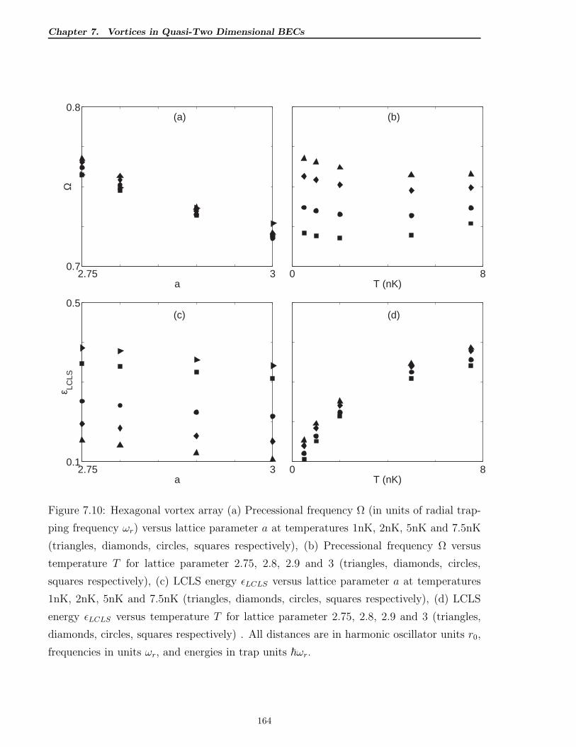
Chapter 7. Vortices in Quasi-Two Dimensional BECs
2.75 30.7
0.8
a
Ω
(a)
0 8T (nK)
(b)
2.75 30.1
0.5
a
ε LCLS
(c)
0 8T (nK)
(d)
Figure 7.10: Hexagonal vortex array (a) Precessional frequency Ω (in units of radial trap-
ping frequency ωr) versus lattice parameter a at temperatures 1nK, 2nK, 5nK and 7.5nK
(triangles, diamonds, circles, squares respectively), (b) Precessional frequency Ω versus
temperature T for lattice parameter 2.75, 2.8, 2.9 and 3 (triangles, diamonds, circles,
squares respectively), (c) LCLS energy ǫLCLS versus lattice parameter a at temperatures
1nK, 2nK, 5nK and 7.5nK (triangles, diamonds, circles, squares respectively), (d) LCLS
energy ǫLCLS versus temperature T for lattice parameter 2.75, 2.8, 2.9 and 3 (triangles,
diamonds, circles, squares respectively) . All distances are in harmonic oscillator units r0,
frequencies in units ωr, and energies in trap units ~ωr.
164
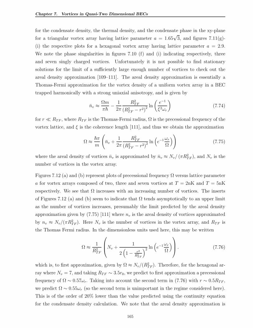
Chapter 7. Vortices in Quasi-Two Dimensional BECs
for the condensate density, the thermal density, and the condensate phase in the xy-plane
for a triangular vortex array having lattice parameter a = 1.65√
3, and figures 7.11(g)-
(i) the respective plots for a hexagonal vortex array having lattice parameter a = 2.9.
We note the phase singularities in figures 7.10 (f) and (i) indicating respectively, three
and seven singly charged vortices. Unfortunately it is not possible to find stationary
solutions for the limit of a sufficiently large enough number of vortices to check out the
areal density approximation [109–111]. The areal density approximation is essentially a
Thomas-Fermi approximation for the vortex density of a uniform vortex array in a BEC
trapped harmonically with a strong uniaxial anisotropy, and is given by
nv ≈Ωm
π~− 1
2π
R2TF
(R2TF − r2)
2 ln
(
e−1
ξ2ωr
)
(7.74)
for r ≪ RTF , where RTF is the Thomas-Fermi radius, Ω is the precessional frequency of the
vortex lattice, and ξ is the coherence length [111], and thus we obtain the approximation
Ω ≈ ~π
m
(
nv +1
2π
R2TF
(R2TF − r2)
2 ln(
e−1ωr
Ω
)
)
(7.75)
where the areal density of vortices nv is approximated by nv ≈ Nv/ (πR2TF ), and Nv is the
number of vortices in the vortex array.
Figures 7.12 (a) and (b) represent plots of precessional frequency Ω versus lattice parameter
a for vortex arrays composed of two, three and seven vortices at T = 2nK and T = 5nK
respectively. We see that Ω increases with an increasing number of vortices. The inserts
of Figures 7.12 (a) and (b) seem to indicate that Ω tends asymptotically to an upper limit
as the number of vortices increases, presumably the limit predicted by the areal density
approximation given by (7.75) [111] where nv is the areal density of vortices approximated
by nv ≈ Nv/(πR2TF ). Here Nv is the number of vortices in the vortex array, and RTF is
the Thomas Fermi radius. In the dimensionless units used here, this may be written
Ω ≈ 1
R2TF
Nv +
1
2(
1− r2
R2TF
)2 ln(
e−1ωr
Ω
)
. (7.76)
which is, to first approximation, given by Ω ≈ Nv/(R2TF ). Therefore, for the hexagonal ar-
ray where Nv = 7, and taking RTF ∼ 3.5r0, we predict to first approximation a precessional
frequency of Ω ∼ 0.57ωr. Taking into account the second term in (7.76) with r ∼ 0.5RTF ,
we predict Ω ∼ 0.55ωr (so the second term is unimportant in the regime considered here).
This is of the order of 20% lower than the value predicted using the continuity equation
for the condensate density calculation. We note that the areal density approximation is
165
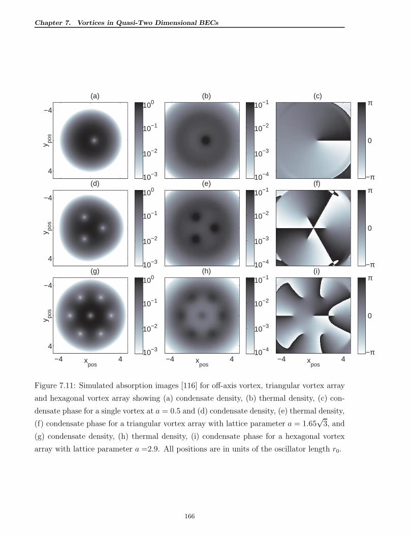
Chapter 7. Vortices in Quasi-Two Dimensional BECs
y pos
(a)100
10−1
10−2
10−3
−4
4
(b)10−1
10−2
10−3
10−4
(c)
π
0
−π
y pos
(d)100
10−1
10−2
10−3
−4
4
(e)10−1
10−2
10−3
10−4
(f)
π
0
−π
xpos
y pos
(g)100
10−1
10−2
10−3
−4 4
−4
4
xpos
(h)10−1
10−2
10−3
10−4
−4 4 xpos
(i) π
0
−π
−4 4
Figure 7.11: Simulated absorption images [116] for off-axis vortex, triangular vortex array
and hexagonal vortex array showing (a) condensate density, (b) thermal density, (c) con-
densate phase for a single vortex at a = 0.5 and (d) condensate density, (e) thermal density,
(f) condensate phase for a triangular vortex array with lattice parameter a = 1.65√
3, and
(g) condensate density, (h) thermal density, (i) condensate phase for a hexagonal vortex
array with lattice parameter a =2.9. All positions are in units of the oscillator length r0.
166
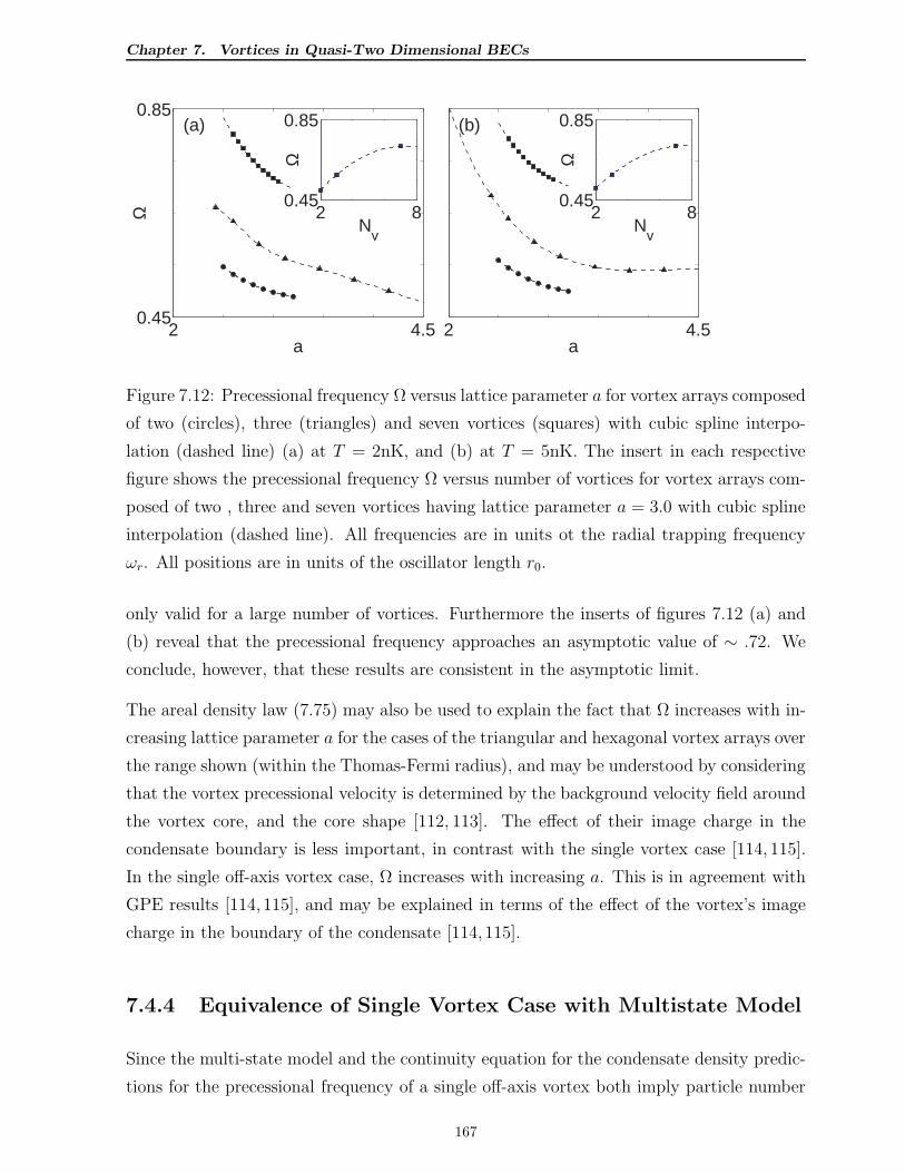
Chapter 7. Vortices in Quasi-Two Dimensional BECs
2 4.50.45
0.85
a
Ω(a)
2 80.45
0.85
Nv
Ω
2 4.5a
(b)
2 80.45
0.85
Nv
Ω
Figure 7.12: Precessional frequency Ω versus lattice parameter a for vortex arrays composed
of two (circles), three (triangles) and seven vortices (squares) with cubic spline interpo-
lation (dashed line) (a) at T = 2nK, and (b) at T = 5nK. The insert in each respective
figure shows the precessional frequency Ω versus number of vortices for vortex arrays com-
posed of two , three and seven vortices having lattice parameter a = 3.0 with cubic spline
interpolation (dashed line). All frequencies are in units ot the radial trapping frequency
ωr. All positions are in units of the oscillator length r0.
only valid for a large number of vortices. Furthermore the inserts of figures 7.12 (a) and
(b) reveal that the precessional frequency approaches an asymptotic value of ∼ .72. We
conclude, however, that these results are consistent in the asymptotic limit.
The areal density law (7.75) may also be used to explain the fact that Ω increases with in-
creasing lattice parameter a for the cases of the triangular and hexagonal vortex arrays over
the range shown (within the Thomas-Fermi radius), and may be understood by considering
that the vortex precessional velocity is determined by the background velocity field around
the vortex core, and the core shape [112, 113]. The effect of their image charge in the
condensate boundary is less important, in contrast with the single vortex case [114, 115].
In the single off-axis vortex case, Ω increases with increasing a. This is in agreement with
GPE results [114, 115], and may be explained in terms of the effect of the vortex’s image
charge in the boundary of the condensate [114, 115].
7.4.4 Equivalence of Single Vortex Case with Multistate Model
Since the multi-state model and the continuity equation for the condensate density predic-
tions for the precessional frequency of a single off-axis vortex both imply particle number
167
Chapter 7. Vortices in Quasi-Two Dimensional BECs
conservation, and the construction of the vortex state in the multi-state is from a com-
plete basis set, and is therefore completely general for the vortex state, one would expect
the two methodologies to yield the same result in the limit of no energy cut-off. Here we
shall demonstrate that this is indeed the case, and that the two representations are ex-
actly equivalent. From (7.49), we see that the time independent solution for the multistate
model in the rotating frame is given by
ΦMS(r, θ) = ag
∑
l 6=1
φ(l)g (r)
eilθ
√2π
+ avφv(r)eiθ
√2π
(7.77)
and for the vortex calculation above by (7.66)
ΦV C(r, θ) =∑
l,n∈S(1)
alnχ(1)ln (r, θ) (7.78)
where χ(1)ln (r, θ) is given by (7.64). The expression for ΦV C(r, θ) given by (7.78) can be
rewritten as
ΦV C(r, θ) =∑
l 6=1
(
∑
n
alnξln(r, θ)
)
eilθ
√2π
+
(
∑
n
alnξ0n(r, θ)−∑
l 6=1
∑
n
alnΛ(1)ln ξ10(r, θ)
)
eiθ
√2π
(7.79)
where Λ(1)ln ≡ ξln(r1, θ1)/ξ10(r1, θ1) for a single off-axis vortex situated at position (r1, θ1).
Comparing expression (7.77) with (7.79), we can identify
agφ(l)g (r) ≡
∑
n
alnξln(r, θ) (7.80)
and
avφv(r) ≡∑
n
alnξ0n(r, θ)−∑
l 6=1
∑
n
alnΛ(1)ln ξ10(r, θ) (7.81)
showing that the two representations are equivalent for a single vortex. We use equation
(7.58) to calculate the precessional frequency ΩMS as predicted by the multi-state model
with the corresponding precessional frequency calculated using the continuity equation
for the condensate density, equation (7.59) for mode cut-off of 100, and of 209. These
are plotted in figure 7.13, and we see that for a sufficient mode cut-off, the agreement is
excellent.
7.5 Two-dimensional Time-dependent Simulations
All time-dependent solutions are done in the interaction picture. We write (ignoring ∆µ,
i.e the shift in the chemical potential due to the fugacity for a finite number of atoms - see
168
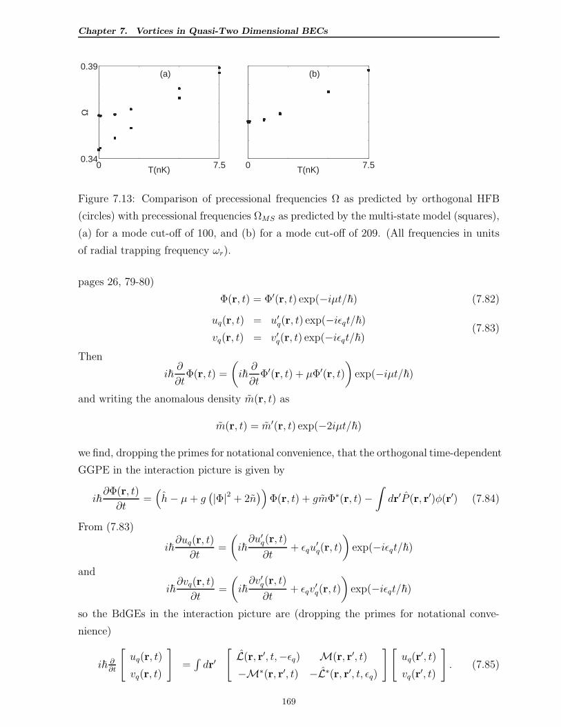
Chapter 7. Vortices in Quasi-Two Dimensional BECs
0 7.50.34
0.39(a)
T(nK)
Ω
0 7.5
(b)
T(nK)
Figure 7.13: Comparison of precessional frequencies Ω as predicted by orthogonal HFB
(circles) with precessional frequencies ΩMS as predicted by the multi-state model (squares),
(a) for a mode cut-off of 100, and (b) for a mode cut-off of 209. (All frequencies in units
of radial trapping frequency ωr).
pages 26, 79-80)
Φ(r, t) = Φ′(r, t) exp(−iµt/~) (7.82)
uq(r, t) = u′q(r, t) exp(−iǫqt/~)
vq(r, t) = v′q(r, t) exp(−iǫqt/~)(7.83)
Then
i~∂
∂tΦ(r, t) =
(
i~∂
∂tΦ′(r, t) + µΦ′(r, t)
)
exp(−iµt/~)
and writing the anomalous density m(r, t) as
m(r, t) = m′(r, t) exp(−2iµt/~)
we find, dropping the primes for notational convenience, that the orthogonal time-dependent
GGPE in the interaction picture is given by
i~∂Φ(r, t)
∂t=(
h− µ+ g(
|Φ|2 + 2n)
)
Φ(r, t) + gmΦ∗(r, t)−∫
dr′P (r, r′)φ(r′) (7.84)
From (7.83)
i~∂uq(r, t)
∂t=
(
i~∂u′q(r, t)
∂t+ ǫqu
′q(r, t)
)
exp(−iǫqt/~)
and
i~∂vq(r, t)
∂t=
(
i~∂v′q(r, t)
∂t+ ǫqv
′q(r, t)
)
exp(−iǫqt/~)
so the BdGEs in the interaction picture are (dropping the primes for notational conve-
nience)
i~ ∂∂t
[
uq(r, t)
vq(r, t)
]
=∫
dr′
[
L(r, r′, t,−ǫq) M(r, r′, t)
−M∗(r, r′, t) −L∗(r, r′, t, ǫq)
][
uq(r′, t)
vq(r′, t)
]
. (7.85)
169
Chapter 7. Vortices in Quasi-Two Dimensional BECs
where
L(r, r′, t, ǫq) ≡ L(r, r′, t) + ǫqδ(r− r′) (7.86)
As pointed out in chapter 4, ∆µ is negligible in the temperature regime of interest, and
can be ignored. Initially all standard HFB time-dependent simulations were done using
the RK4IP algorithm [90, 105] (see chapter 5, sections 5.4.1, 5.4.2 for a summary), but
with the need to implement the orthogonal formalism5 (7.84) and (7.85), a new fourth
order Runge-Kutta algorithm based on the evolution of the coefficients of the condensate
wave function, and of the quasiparticle amplitudes expanded in the Laguerre basis was
implemented (see chapter 5, section 5.4.3 for a description of the algorithm). This algorithm
has the advantage that it permits a much larger energy cut-off, and also runs quicker, in
view of the Gaussian grid which is much smaller than the Fourier grid required for the
RK4IP algorithm - see chapter 5, section 5.4.3 for a comparison. The results obtained
with each method are comparable - see chapter 5, section 5.4.3 on numerical methods.
7.5.1 Evolution of Time-independent Solutions
Time-dependent simulations were done for the standard HFB for T = 5nK for a vortex at
a = 0.5 radial harmonic oscillator units from the axis, with a mode cutoff of 100, using the
time-independent data initial state. In all the simulations, the vortex precession describes a
circle. The precessional frequency was estimated using a least squares fit of a sinusoid to the
vortex x-displacement versus time, and was found to be ΩLS = 0.3794ωr, in good agreement
with the value of Ω = 0.3727ωr, as predicted in the time-independent calculations. The
error in the prediction scales as the number of computational basis functions6 which, for
practical reasons, is only 209 in these calculations. Calculations for the single off-axis
vortex taking the projector P into account, presented in appendix F.3 predict a value of
Ω = 0.3756ωr. For 839 computational basis functions, the time-independent calculations
predict a value of Ω = 0.3761ωr. We see no evidence of dissipation during the time of the
simulation of ten trap cycles. Examination of the plot of the x-displacement versus time
(in trap cycles) in figure 7.14(a) reveals that this is indeed the case. Figure 7.14(b) shows
that the trajectory of the vortex constitutes a circle.
5See comments on use of standard time-dependent HFB versus orthogonal time-dependent HFB at end
of section 5.4.6Clearly it would be desirable to increase the mode cut-off. However, for practical reasons, these are
limited to 100, since these results are still reasonably accurate (∼ 2%) and to increase this number would
significantly increase the computational effort, rendering these calculations impractical. These results can
be refined, but the computation required is formidable.
170
Chapter 7. Vortices in Quasi-Two Dimensional BECs
Time-dependent simulations were also done for the standard HFB for T = 5nK for a
symmetrical triangular vortex array with lattice parameter a = 1.65√
3 (i.e. three vortices
symmetrically positioned at 1.65 radial harmonic oscillator units from the axis), and for
a symmetrical hexagonal triangular vortex centred on the axis having lattice parameter
a = 2.85 (i.e. seven vortices), again using time-independent calculations for the initial state.
For this symmetric case, all vortices precess in the same way with phase differences of 2π/3
and π/3 for the triangular and hexagonal vortex arrays respectively, with the exception of
the central vortex in the hexagonal array, which remains fixed. In both simulations, the
vortex precession describes a circle. Again we see no evidence of dissipation during the time
of the simulation of five trap cycles. Examination of the plots of the x-displacement versus
time (in trap cycles) in figures 7.14(c) and 7.14(e), where we have selected a representative
vortex for display purposes, reveals that this is indeed the case. The precessional frequency
for the triangular vortex array was estimated using a least squares fit of a sinusoid to
the vortex x-displacement versus time of a representative vortex, and was found to be
ΩLS = 0.5856ωr, in good agreement with the value of Ω = 0.5938ωr, as predicted in
the time-independent calculations for 209 computational basis functions. Figures 7.14(d)
and 7.14(f) show, respectively the trajectories of the representative vortices, which both
constitute a circle.
7.5.2 Stirring of the Condensate
In these simulations we use one or more Gaussian stirrers in order to stir the condensate.
The stirring imparts angular momentum to the condensate, and therefore one would expect
the production of vortices in cases where the angular frequency of the stirrer(s) exceeds a
certain critical value. This should correspond (at least approximately) to the velocity of
the stirrer with respect to the stirrer exceeding the local Landau critical velocity (i.e. the
local speed of sound). In what follows we shall establish a critical stirring frequency, below
which no vortices are produced in regions of appreciable density (i.e. within the Thomas-
Fermi radius). In these simulations we find that this critical frequency corresponds to a
velocity of the stirrer through the BEC that is slightly in excess of the local Landau critical
velocity7 (see table 7.1).
7This may be explained by noting the following: The expression s =√
ng/m for the “speed of sound”
is that appropriate to the Bogoliubov approximation (and the HFB-Popov approximation). In the HFB
case, however, the spectrum is steepened by the presence of the anomalous density (see equation (44) of
Griffin [11]), and is not linear in k as k → 0 anyway, due to the presence of the gap. Thus the critical
velocity obtained from the fundamental Landau definition Vc = min (E(k)/k) will be raised above the
171
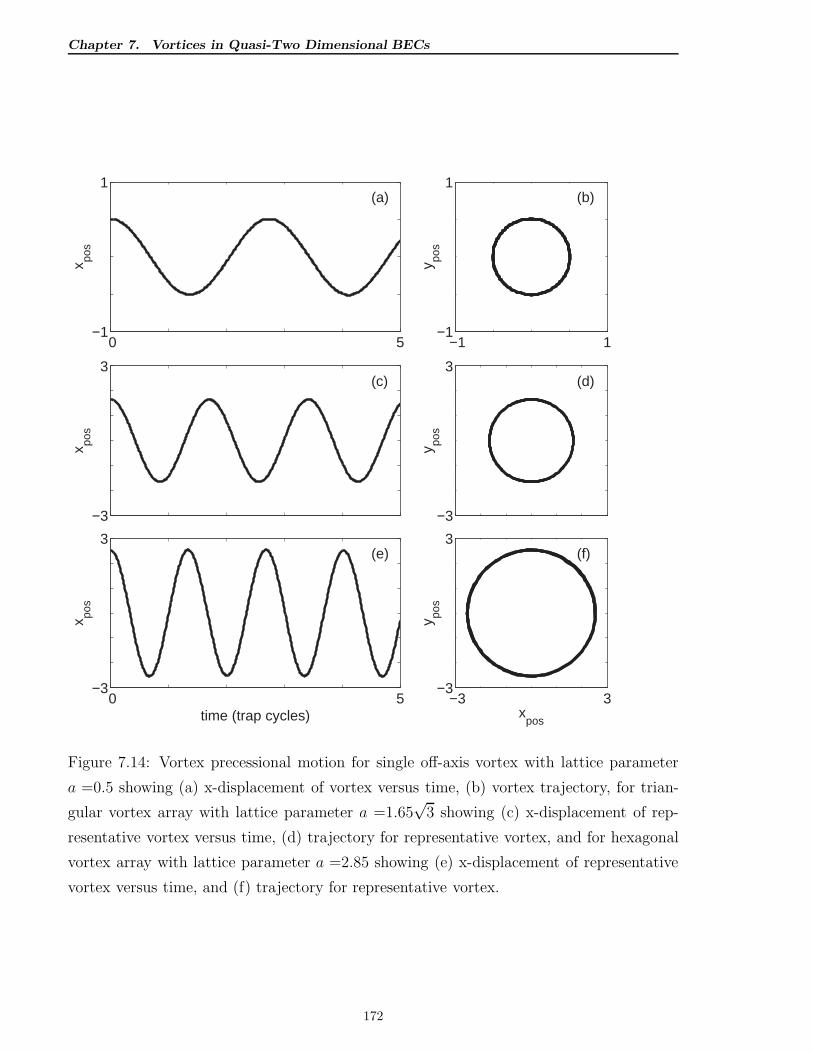
Chapter 7. Vortices in Quasi-Two Dimensional BECs
0 5 −1
1
x pos
(a)
−1 1−1
1
y pos
(b)
−3
3
x pos
(c)
−3
3
y pos
(d)
0 5 −3
3
time (trap cycles)
x pos
(e)
−3 3−3
3
xpos
y pos
(f)
Figure 7.14: Vortex precessional motion for single off-axis vortex with lattice parameter
a =0.5 showing (a) x-displacement of vortex versus time, (b) vortex trajectory, for trian-
gular vortex array with lattice parameter a =1.65√
3 showing (c) x-displacement of rep-
resentative vortex versus time, (d) trajectory for representative vortex, and for hexagonal
vortex array with lattice parameter a =2.85 showing (e) x-displacement of representative
vortex versus time, and (f) trajectory for representative vortex.
172
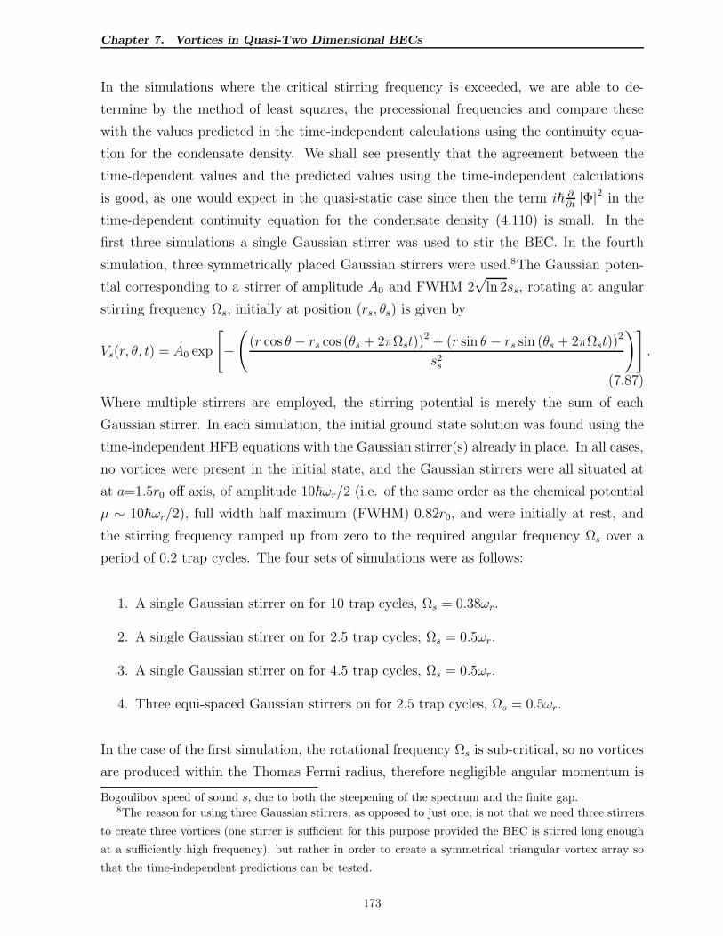
Chapter 7. Vortices in Quasi-Two Dimensional BECs
In the simulations where the critical stirring frequency is exceeded, we are able to de-
termine by the method of least squares, the precessional frequencies and compare these
with the values predicted in the time-independent calculations using the continuity equa-
tion for the condensate density. We shall see presently that the agreement between the
time-dependent values and the predicted values using the time-independent calculations
is good, as one would expect in the quasi-static case since then the term i~ ∂∂t|Φ|2 in the
time-dependent continuity equation for the condensate density (4.110) is small. In the
first three simulations a single Gaussian stirrer was used to stir the BEC. In the fourth
simulation, three symmetrically placed Gaussian stirrers were used.8The Gaussian poten-
tial corresponding to a stirrer of amplitude A0 and FWHM 2√
ln 2ss, rotating at angular
stirring frequency Ωs, initially at position (rs, θs) is given by
Vs(r, θ, t) = A0 exp
[
−(
(r cos θ − rs cos (θs + 2πΩst))2 + (r sin θ − rs sin (θs + 2πΩst))
2
s2s
)]
.
(7.87)
Where multiple stirrers are employed, the stirring potential is merely the sum of each
Gaussian stirrer. In each simulation, the initial ground state solution was found using the
time-independent HFB equations with the Gaussian stirrer(s) already in place. In all cases,
no vortices were present in the initial state, and the Gaussian stirrers were all situated at
at a=1.5r0 off axis, of amplitude 10~ωr/2 (i.e. of the same order as the chemical potential
µ ∼ 10~ωr/2), full width half maximum (FWHM) 0.82r0, and were initially at rest, and
the stirring frequency ramped up from zero to the required angular frequency Ωs over a
period of 0.2 trap cycles. The four sets of simulations were as follows:
1. A single Gaussian stirrer on for 10 trap cycles, Ωs = 0.38ωr.
2. A single Gaussian stirrer on for 2.5 trap cycles, Ωs = 0.5ωr.
3. A single Gaussian stirrer on for 4.5 trap cycles, Ωs = 0.5ωr.
4. Three equi-spaced Gaussian stirrers on for 2.5 trap cycles, Ωs = 0.5ωr.
In the case of the first simulation, the rotational frequency Ωs is sub-critical, so no vortices
are produced within the Thomas Fermi radius, therefore negligible angular momentum is
Bogoulibov speed of sound s, due to both the steepening of the spectrum and the finite gap.8The reason for using three Gaussian stirrers, as opposed to just one, is not that we need three stirrers
to create three vortices (one stirrer is sufficient for this purpose provided the BEC is stirred long enough
at a sufficiently high frequency), but rather in order to create a symmetrical triangular vortex array so
that the time-independent predictions can be tested.
173
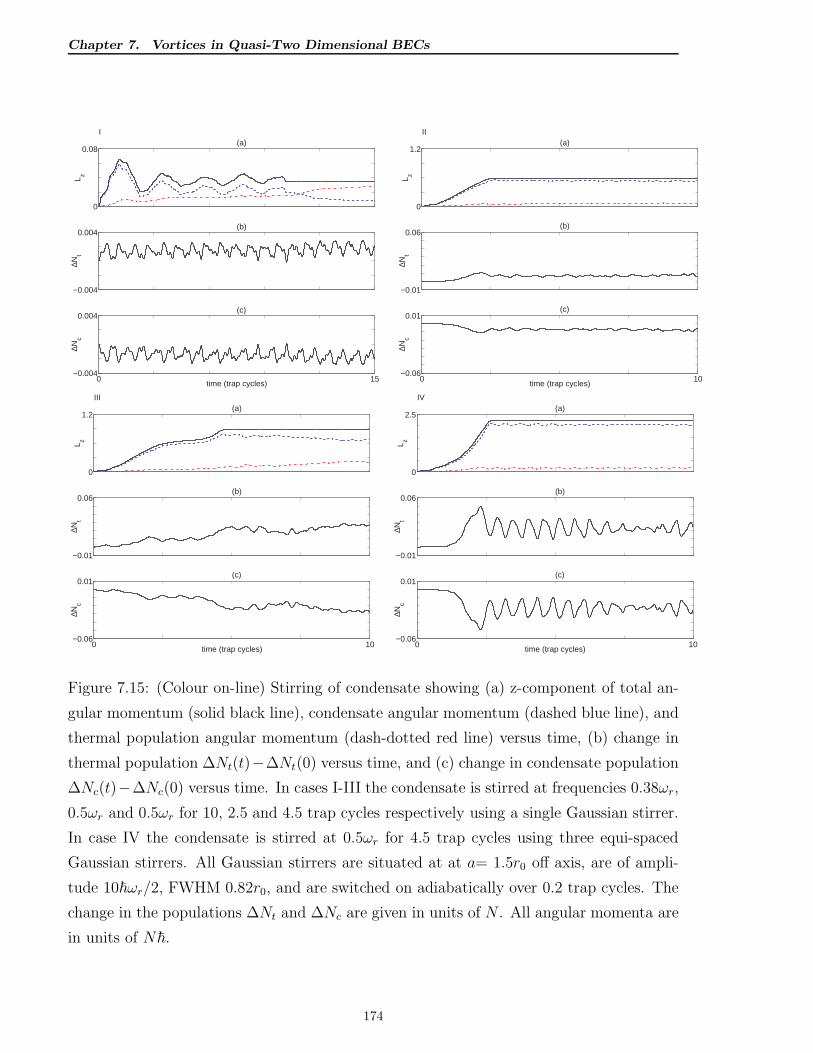
Chapter 7. Vortices in Quasi-Two Dimensional BECs
0
0.08
L z
I(a)
−0.004
0.004
∆Nt
(b)
0 15−0.004
0.004
time (trap cycles)
∆Nc
(c)
0
1.2
L z
II(a)
−0.01
0.06
∆Nt
(b)
0 10−0.06
0.01
time (trap cycles)
∆Nc
(c)
0
1.2
L z
III(a)
−0.01
0.06
∆Nt
(b)
0 10−0.06
0.01
time (trap cycles)
∆Nc
(c)
0
2.5
L zIV
(a)
−0.01
0.06
∆Nt
(b)
0 10−0.06
0.01
time (trap cycles)
∆Nc
(c)
Figure 7.15: (Colour on-line) Stirring of condensate showing (a) z-component of total an-
gular momentum (solid black line), condensate angular momentum (dashed blue line), and
thermal population angular momentum (dash-dotted red line) versus time, (b) change in
thermal population ∆Nt(t)−∆Nt(0) versus time, and (c) change in condensate population
∆Nc(t)−∆Nc(0) versus time. In cases I-III the condensate is stirred at frequencies 0.38ωr,
0.5ωr and 0.5ωr for 10, 2.5 and 4.5 trap cycles respectively using a single Gaussian stirrer.
In case IV the condensate is stirred at 0.5ωr for 4.5 trap cycles using three equi-spaced
Gaussian stirrers. All Gaussian stirrers are situated at at a= 1.5r0 off axis, are of ampli-
tude 10~ωr/2, FWHM 0.82r0, and are switched on adiabatically over 0.2 trap cycles. The
change in the populations ∆Nt and ∆Nc are given in units of N . All angular momenta are
in units of N~.
174
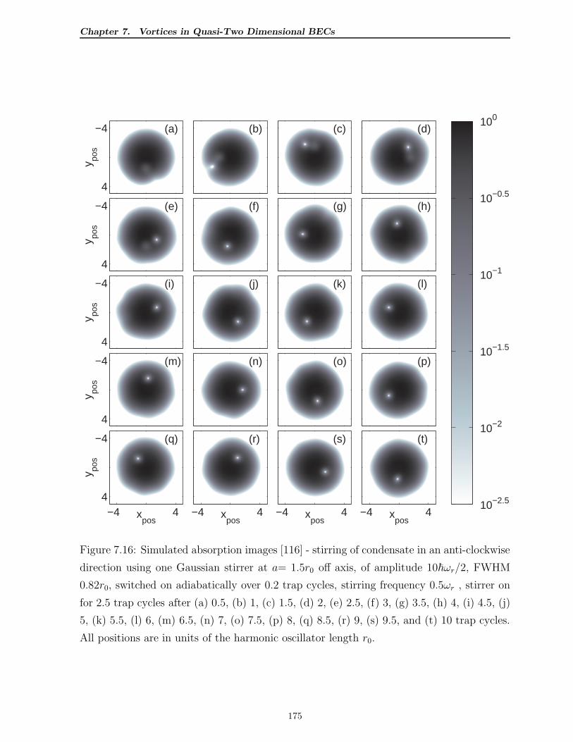
Chapter 7. Vortices in Quasi-Two Dimensional BECs
y pos
(a)−4
4
(b) (c) (d)
y pos
(e)−4
4
(f) (g) (h)
y pos
(i)−4
4
(j) (k) (l)
y pos
(m)−4
4
(n) (o) (p)
xpos
y pos
(q)
−4 4
−4
4
xpos
(r)
−4 4 xpos
(s)
−4 4 xpos
(t)
100
10−0.5
10−1
10−1.5
10−2
10−2.5
−4 4
Figure 7.16: Simulated absorption images [116] - stirring of condensate in an anti-clockwise
direction using one Gaussian stirrer at a= 1.5r0 off axis, of amplitude 10~ωr/2, FWHM
0.82r0, switched on adiabatically over 0.2 trap cycles, stirring frequency 0.5ωr , stirrer on
for 2.5 trap cycles after (a) 0.5, (b) 1, (c) 1.5, (d) 2, (e) 2.5, (f) 3, (g) 3.5, (h) 4, (i) 4.5, (j)
5, (k) 5.5, (l) 6, (m) 6.5, (n) 7, (o) 7.5, (p) 8, (q) 8.5, (r) 9, (s) 9.5, and (t) 10 trap cycles.
All positions are in units of the harmonic oscillator length r0.
175
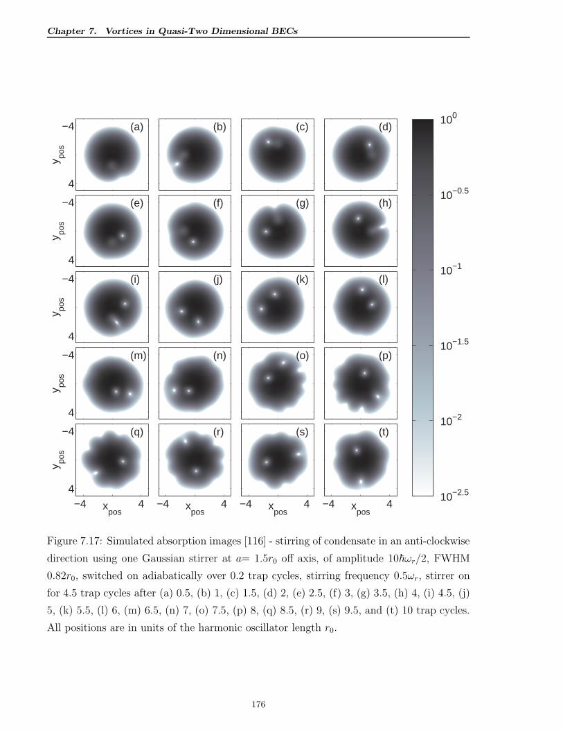
Chapter 7. Vortices in Quasi-Two Dimensional BECs
y pos
(a)−4
4
(b) (c) (d)
y pos
(e)−4
4
(f) (g) (h)
y pos
(i)−4
4
(j) (k) (l)
y pos
(m)−4
4
(n) (o) (p)
xpos
y pos
(q)
−4 4
−4
4
xpos
(r)
−4 4 xpos
(s)
−4 4 xpos
(t)
100
10−0.5
10−1
10−1.5
10−2
10−2.5
−4 4
Figure 7.17: Simulated absorption images [116] - stirring of condensate in an anti-clockwise
direction using one Gaussian stirrer at a= 1.5r0 off axis, of amplitude 10~ωr/2, FWHM
0.82r0, switched on adiabatically over 0.2 trap cycles, stirring frequency 0.5ωr, stirrer on
for 4.5 trap cycles after (a) 0.5, (b) 1, (c) 1.5, (d) 2, (e) 2.5, (f) 3, (g) 3.5, (h) 4, (i) 4.5, (j)
5, (k) 5.5, (l) 6, (m) 6.5, (n) 7, (o) 7.5, (p) 8, (q) 8.5, (r) 9, (s) 9.5, and (t) 10 trap cycles.
All positions are in units of the harmonic oscillator length r0.
176
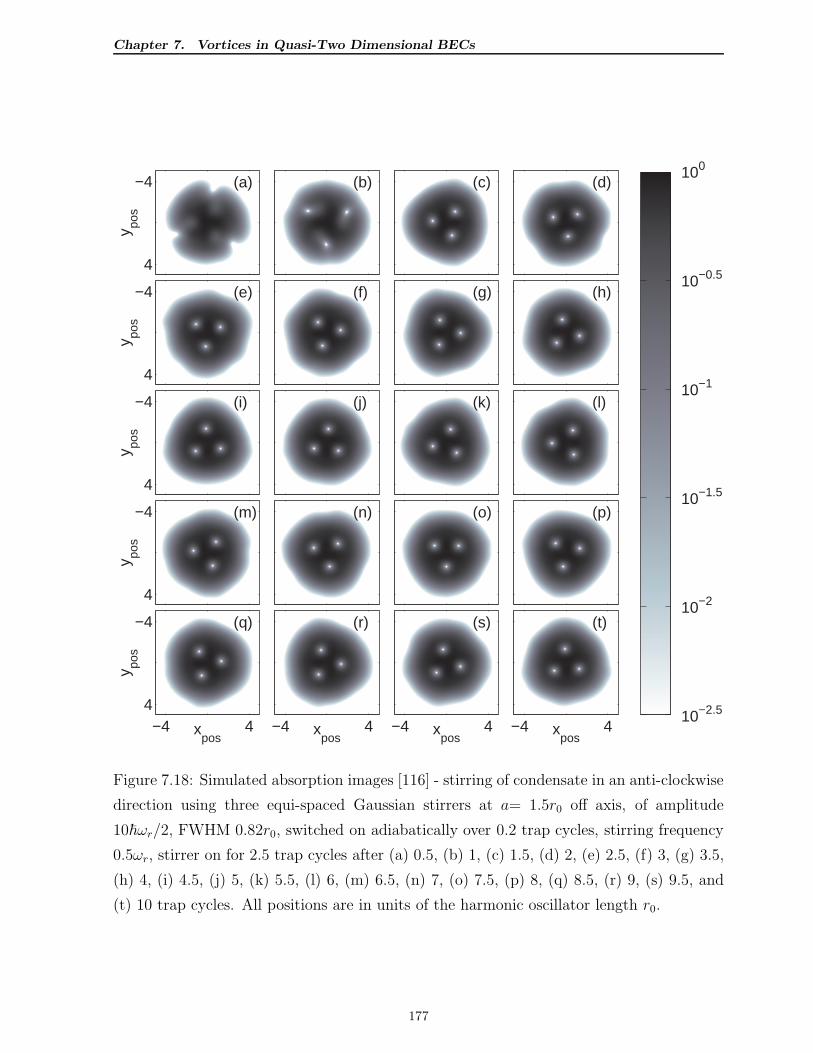
Chapter 7. Vortices in Quasi-Two Dimensional BECs
y pos
(a)−4
4
(b) (c) (d)
y pos
(e)−4
4
(f) (g) (h)
y pos
(i)−4
4
(j) (k) (l)
y pos
(m)−4
4
(n) (o) (p)
xpos
y pos
(q)
−4 4
−4
4
xpos
(r)
−4 4 xpos
(s)
−4 4 xpos
(t)
100
10−0.5
10−1
10−1.5
10−2
10−2.5
−4 4
Figure 7.18: Simulated absorption images [116] - stirring of condensate in an anti-clockwise
direction using three equi-spaced Gaussian stirrers at a= 1.5r0 off axis, of amplitude
10~ωr/2, FWHM 0.82r0, switched on adiabatically over 0.2 trap cycles, stirring frequency
0.5ωr, stirrer on for 2.5 trap cycles after (a) 0.5, (b) 1, (c) 1.5, (d) 2, (e) 2.5, (f) 3, (g) 3.5,
(h) 4, (i) 4.5, (j) 5, (k) 5.5, (l) 6, (m) 6.5, (n) 7, (o) 7.5, (p) 8, (q) 8.5, (r) 9, (s) 9.5, and
(t) 10 trap cycles. All positions are in units of the harmonic oscillator length r0.
177
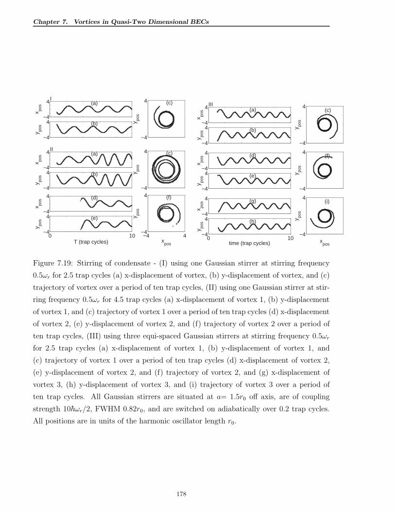
Chapter 7. Vortices in Quasi-Two Dimensional BECs
−4
4
x pos
I(a)
−4
4
y pos (b)
−4
4
x pos
II(a)
−4
4
y pos (b)
−4
4
x pos (d)
0 10−4
4
T (trap cycles)
y pos (e)
−4
4
y pos
(c)
−4
4
y pos
(c)
−4 4−4
4
xpos
y pos
(f)
−4
4
x pos
III(a)
−4
4
y pos (b)
−4
4
x pos (d)
−4
4
y pos (e)
−4
4x po
s (g)
0 10−4
4
time (trap cycles)
y pos (h)
−4
4
y pos
(c)
−4
4
y pos
(f)
−4
4
xpos
y pos
(i)
Figure 7.19: Stirring of condensate - (I) using one Gaussian stirrer at stirring frequency
0.5ωr for 2.5 trap cycles (a) x-displacement of vortex, (b) y-displacement of vortex, and (c)
trajectory of vortex over a period of ten trap cycles, (II) using one Gaussian stirrer at stir-
ring frequency 0.5ωr for 4.5 trap cycles (a) x-displacement of vortex 1, (b) y-displacement
of vortex 1, and (c) trajectory of vortex 1 over a period of ten trap cycles (d) x-displacement
of vortex 2, (e) y-displacement of vortex 2, and (f) trajectory of vortex 2 over a period of
ten trap cycles, (III) using three equi-spaced Gaussian stirrers at stirring frequency 0.5ωr
for 2.5 trap cycles (a) x-displacement of vortex 1, (b) y-displacement of vortex 1, and
(c) trajectory of vortex 1 over a period of ten trap cycles (d) x-displacement of vortex 2,
(e) y-displacement of vortex 2, and (f) trajectory of vortex 2, and (g) x-displacement of
vortex 3, (h) y-displacement of vortex 3, and (i) trajectory of vortex 3 over a period of
ten trap cycles. All Gaussian stirrers are situated at a= 1.5r0 off axis, are of coupling
strength 10~ωr/2, FWHM 0.82r0, and are switched on adiabatically over 0.2 trap cycles.
All positions are in units of the harmonic oscillator length r0.
178
Chapter 7. Vortices in Quasi-Two Dimensional BECs
transferred to the condensate. This angular momentum is due to circulation corresponding
to vortices in regions of neglible density9. A small amount of angular momentum is also
transferred to the thermal cloud. This accounts for the small amount of angular momentum
in the condensate and in the thermal population as shown in figure 7.15 I(a) which is a
plot of the z-component of the angular momentum versus time. We note that Lz remains
fixed once the stirring ceases after 10.2 trap cycles in accordance with the conservation
of angular momentum. We note that the angular momentum for the thermal population
increases for the first few trap cycles, reaching a saturation value after ∼ 4 → 5 trap
cycles. Simulations over a much longer time scale (not presented here) reveal a slow cyclical
change in the thermal population angular momentum of a few percent. Once the stirrer
is switched off, we see a steady increase in the thermal population angular momentum
with a resultant loss in the angular momentum of the condensate (since the overall angular
momentum is conserved). During the time of stirring, the condensate angular momentum
varies cyclically corresponding to the variation of vortices from the axis (see also [90,105]).
In the case where the stirring frequency is sub-critical, these vortices would lie outside
the Thomas Fermi radius and would therefore be sub-threshold. Figures 7.15 I(b),(c)
show respectively the changes in condensate and thermal density, where we see rigorous
observance of particle number conservation. In simulations two and three, the stirring
frequency Ωs is sufficient for the production of vortices, and figures 7.16 (a)-(t) and figures
7.17 (a)-(t) show the respective simulated absorption images. Figures 7.18 (a)-(t) represent
simulated absorption images for the fourth simulation using three Gaussian stirrers. In the
second sequence, only one vortex is created, and its x-displacement xpos and y-displacement
ypos versus time in trap cycles shown in figures 7.19 I(a),(b), and its trajectory in figure
7.19 I(c) [117]. In all four cases we see evidence of heating as the condensate is stirred in
figure 7.15 in panels I(b), II(b), III(b), and IV(b), which each indicate an increase in the
thermal population. In order to understand why there exists a critical frequency for the
production of vortices within the Thomas Fermi radius, we calculate the Landau critical
velocity vLC given by the speed of sound at the point of the stirrer s =√
ng/m where n
is the density of the superfluid, and m is the mass of a particle. We use the local density
approximation, and calculate the speed of sound s at the stirrer using the local density n
of the superfluid at the point of the stirrer.
In these simulations, we measure the two-dimensional density n(2D) where we have inte-
9This angular momentum is due to circulation of the condensate in regions of vanishing density, and is
at least an order of magnitude smaller than in situations where the stirring frequency exceeds the critical
value, and vortices can be produced in regions of appreciable density (i.e within the Thomas Fermi radius).
179
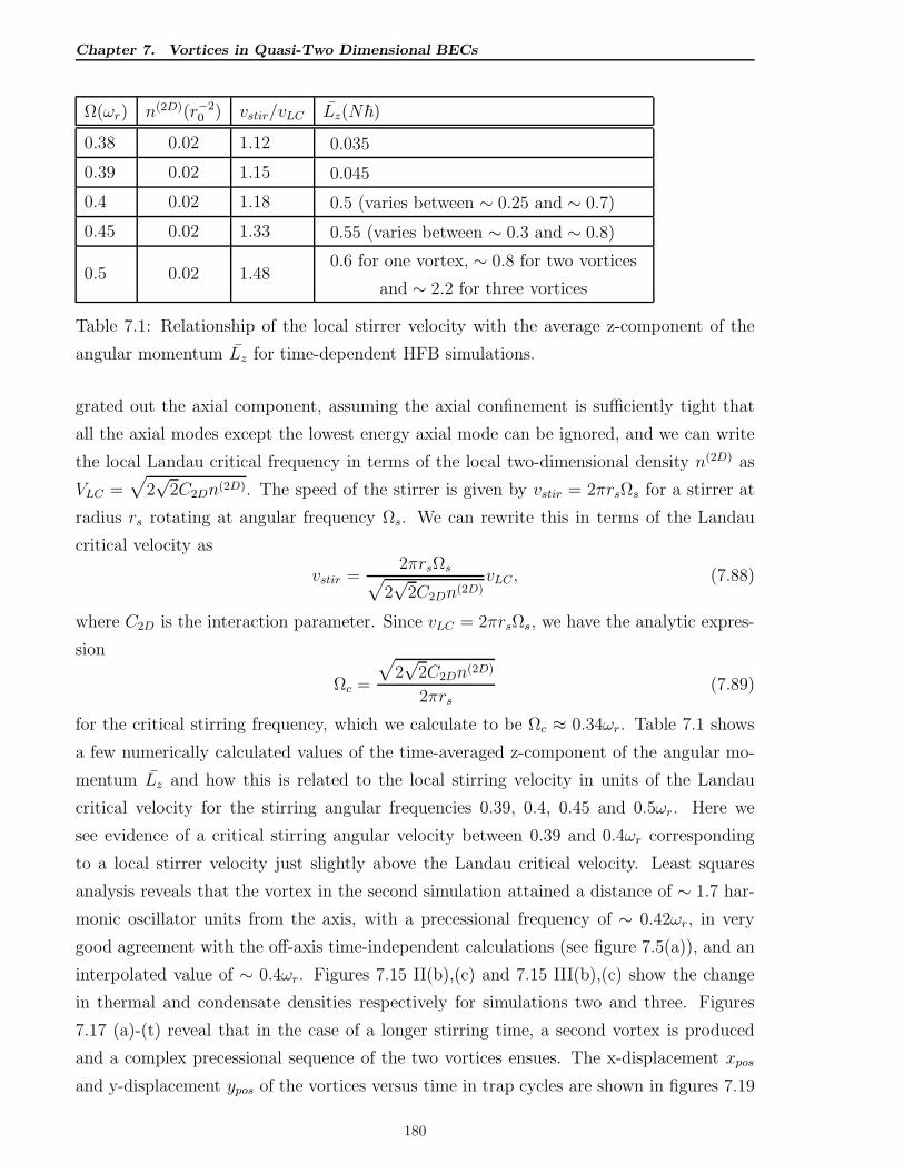
Chapter 7. Vortices in Quasi-Two Dimensional BECs
Ω(ωr) n(2D)(r−20 ) vstir/vLC Lz(N~)
0.38 0.02 1.12 0.035
0.39 0.02 1.15 0.045
0.4 0.02 1.18 0.5 (varies between ∼ 0.25 and ∼ 0.7)
0.45 0.02 1.33 0.55 (varies between ∼ 0.3 and ∼ 0.8)
0.5 0.02 1.480.6 for one vortex, ∼ 0.8 for two vortices
and ∼ 2.2 for three vortices
Table 7.1: Relationship of the local stirrer velocity with the average z-component of the
angular momentum Lz for time-dependent HFB simulations.
grated out the axial component, assuming the axial confinement is sufficiently tight that
all the axial modes except the lowest energy axial mode can be ignored, and we can write
the local Landau critical frequency in terms of the local two-dimensional density n(2D) as
VLC =√
2√
2C2Dn(2D). The speed of the stirrer is given by vstir = 2πrsΩs for a stirrer at
radius rs rotating at angular frequency Ωs. We can rewrite this in terms of the Landau
critical velocity as
vstir =2πrsΩs
√
2√
2C2Dn(2D)vLC , (7.88)
where C2D is the interaction parameter. Since vLC = 2πrsΩs, we have the analytic expres-
sion
Ωc =
√
2√
2C2Dn(2D)
2πrs(7.89)
for the critical stirring frequency, which we calculate to be Ωc ≈ 0.34ωr. Table 7.1 shows
a few numerically calculated values of the time-averaged z-component of the angular mo-
mentum Lz and how this is related to the local stirring velocity in units of the Landau
critical velocity for the stirring angular frequencies 0.39, 0.4, 0.45 and 0.5ωr. Here we
see evidence of a critical stirring angular velocity between 0.39 and 0.4ωr corresponding
to a local stirrer velocity just slightly above the Landau critical velocity. Least squares
analysis reveals that the vortex in the second simulation attained a distance of ∼ 1.7 har-
monic oscillator units from the axis, with a precessional frequency of ∼ 0.42ωr, in very
good agreement with the off-axis time-independent calculations (see figure 7.5(a)), and an
interpolated value of ∼ 0.4ωr. Figures 7.15 II(b),(c) and 7.15 III(b),(c) show the change
in thermal and condensate densities respectively for simulations two and three. Figures
7.17 (a)-(t) reveal that in the case of a longer stirring time, a second vortex is produced
and a complex precessional sequence of the two vortices ensues. The x-displacement xpos
and y-displacement ypos of the vortices versus time in trap cycles are shown in figures 7.19
180
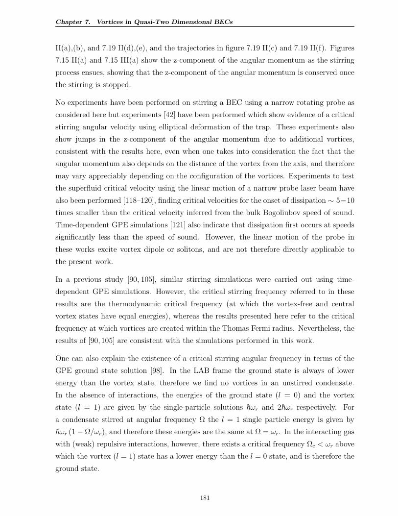
Chapter 7. Vortices in Quasi-Two Dimensional BECs
II(a),(b), and 7.19 II(d),(e), and the trajectories in figure 7.19 II(c) and 7.19 II(f). Figures
7.15 II(a) and 7.15 III(a) show the z-component of the angular momentum as the stirring
process ensues, showing that the z-component of the angular momentum is conserved once
the stirring is stopped.
No experiments have been performed on stirring a BEC using a narrow rotating probe as
considered here but experiments [42] have been performed which show evidence of a critical
stirring angular velocity using elliptical deformation of the trap. These experiments also
show jumps in the z-component of the angular momentum due to additional vortices,
consistent with the results here, even when one takes into consideration the fact that the
angular momentum also depends on the distance of the vortex from the axis, and therefore
may vary appreciably depending on the configuration of the vortices. Experiments to test
the superfluid critical velocity using the linear motion of a narrow probe laser beam have
also been performed [118–120], finding critical velocities for the onset of dissipation ∼ 5−10
times smaller than the critical velocity inferred from the bulk Bogoliubov speed of sound.
Time-dependent GPE simulations [121] also indicate that dissipation first occurs at speeds
significantly less than the speed of sound. However, the linear motion of the probe in
these works excite vortex dipole or solitons, and are not therefore directly applicable to
the present work.
In a previous study [90, 105], similar stirring simulations were carried out using time-
dependent GPE simulations. However, the critical stirring frequency referred to in these
results are the thermodynamic critical frequency (at which the vortex-free and central
vortex states have equal energies), whereas the results presented here refer to the critical
frequency at which vortices are created within the Thomas Fermi radius. Nevertheless, the
results of [90, 105] are consistent with the simulations performed in this work.
One can also explain the existence of a critical stirring angular frequency in terms of the
GPE ground state solution [98]. In the LAB frame the ground state is always of lower
energy than the vortex state, therefore we find no vortices in an unstirred condensate.
In the absence of interactions, the energies of the ground state (l = 0) and the vortex
state (l = 1) are given by the single-particle solutions ~ωr and 2~ωr respectively. For
a condensate stirred at angular frequency Ω the l = 1 single particle energy is given by
~ωr (1− Ω/ωr), and therefore these energies are the same at Ω = ωr. In the interacting gas
with (weak) repulsive interactions, however, there exists a critical frequency Ωc < ωr above
which the vortex (l = 1) state has a lower energy than the l = 0 state, and is therefore the
ground state.
181
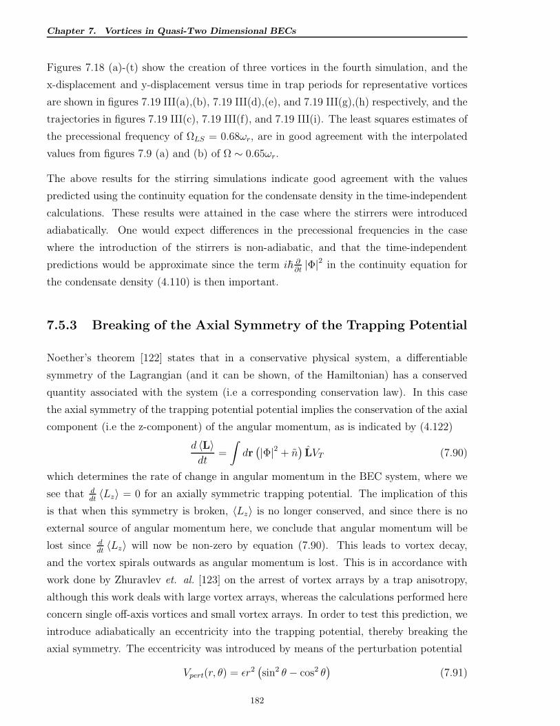
Chapter 7. Vortices in Quasi-Two Dimensional BECs
Figures 7.18 (a)-(t) show the creation of three vortices in the fourth simulation, and the
x-displacement and y-displacement versus time in trap periods for representative vortices
are shown in figures 7.19 III(a),(b), 7.19 III(d),(e), and 7.19 III(g),(h) respectively, and the
trajectories in figures 7.19 III(c), 7.19 III(f), and 7.19 III(i). The least squares estimates of
the precessional frequency of ΩLS = 0.68ωr, are in good agreement with the interpolated
values from figures 7.9 (a) and (b) of Ω ∼ 0.65ωr.
The above results for the stirring simulations indicate good agreement with the values
predicted using the continuity equation for the condensate density in the time-independent
calculations. These results were attained in the case where the stirrers were introduced
adiabatically. One would expect differences in the precessional frequencies in the case
where the introduction of the stirrers is non-adiabatic, and that the time-independent
predictions would be approximate since the term i~ ∂∂t|Φ|2 in the continuity equation for
the condensate density (4.110) is then important.
7.5.3 Breaking of the Axial Symmetry of the Trapping Potential
Noether’s theorem [122] states that in a conservative physical system, a differentiable
symmetry of the Lagrangian (and it can be shown, of the Hamiltonian) has a conserved
quantity associated with the system (i.e a corresponding conservation law). In this case
the axial symmetry of the trapping potential potential implies the conservation of the axial
component (i.e the z-component) of the angular momentum, as is indicated by (4.122)
d 〈L〉dt
=
∫
dr(
|Φ|2 + n)
LVT (7.90)
which determines the rate of change in angular momentum in the BEC system, where we
see that ddt〈Lz〉 = 0 for an axially symmetric trapping potential. The implication of this
is that when this symmetry is broken, 〈Lz〉 is no longer conserved, and since there is no
external source of angular momentum here, we conclude that angular momentum will be
lost since ddt〈Lz〉 will now be non-zero by equation (7.90). This leads to vortex decay,
and the vortex spirals outwards as angular momentum is lost. This is in accordance with
work done by Zhuravlev et. al. [123] on the arrest of vortex arrays by a trap anisotropy,
although this work deals with large vortex arrays, whereas the calculations performed here
concern single off-axis vortices and small vortex arrays. In order to test this prediction, we
introduce adiabatically an eccentricity into the trapping potential, thereby breaking the
axial symmetry. The eccentricity was introduced by means of the perturbation potential
Vpert(r, θ) = ǫr2(
sin2 θ − cos2 θ)
(7.91)
182
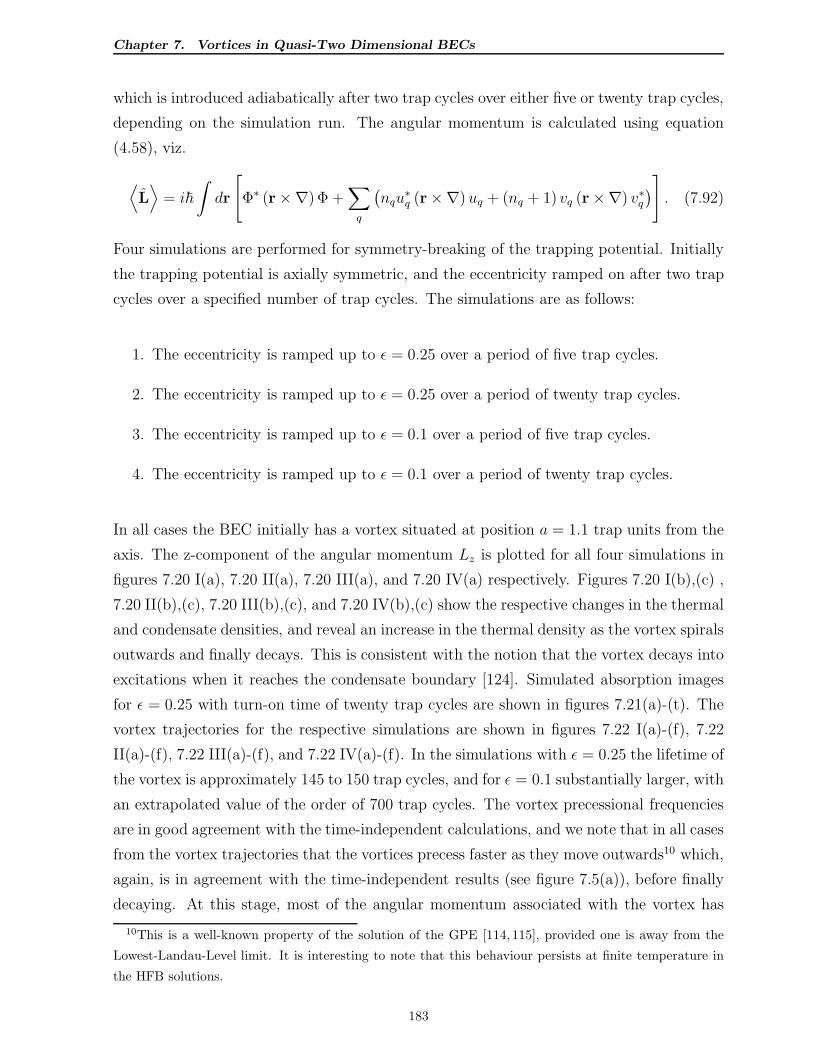
Chapter 7. Vortices in Quasi-Two Dimensional BECs
which is introduced adiabatically after two trap cycles over either five or twenty trap cycles,
depending on the simulation run. The angular momentum is calculated using equation
(4.58), viz.
⟨
L⟩
= i~
∫
dr
[
Φ∗ (r×∇)Φ +∑
q
(
nqu∗q (r×∇) uq + (nq + 1) vq (r×∇) v∗q
)
]
. (7.92)
Four simulations are performed for symmetry-breaking of the trapping potential. Initially
the trapping potential is axially symmetric, and the eccentricity ramped on after two trap
cycles over a specified number of trap cycles. The simulations are as follows:
1. The eccentricity is ramped up to ǫ = 0.25 over a period of five trap cycles.
2. The eccentricity is ramped up to ǫ = 0.25 over a period of twenty trap cycles.
3. The eccentricity is ramped up to ǫ = 0.1 over a period of five trap cycles.
4. The eccentricity is ramped up to ǫ = 0.1 over a period of twenty trap cycles.
In all cases the BEC initially has a vortex situated at position a = 1.1 trap units from the
axis. The z-component of the angular momentum Lz is plotted for all four simulations in
figures 7.20 I(a), 7.20 II(a), 7.20 III(a), and 7.20 IV(a) respectively. Figures 7.20 I(b),(c) ,
7.20 II(b),(c), 7.20 III(b),(c), and 7.20 IV(b),(c) show the respective changes in the thermal
and condensate densities, and reveal an increase in the thermal density as the vortex spirals
outwards and finally decays. This is consistent with the notion that the vortex decays into
excitations when it reaches the condensate boundary [124]. Simulated absorption images
for ǫ = 0.25 with turn-on time of twenty trap cycles are shown in figures 7.21(a)-(t). The
vortex trajectories for the respective simulations are shown in figures 7.22 I(a)-(f), 7.22
II(a)-(f), 7.22 III(a)-(f), and 7.22 IV(a)-(f). In the simulations with ǫ = 0.25 the lifetime of
the vortex is approximately 145 to 150 trap cycles, and for ǫ = 0.1 substantially larger, with
an extrapolated value of the order of 700 trap cycles. The vortex precessional frequencies
are in good agreement with the time-independent calculations, and we note that in all cases
from the vortex trajectories that the vortices precess faster as they move outwards10 which,
again, is in agreement with the time-independent results (see figure 7.5(a)), before finally
decaying. At this stage, most of the angular momentum associated with the vortex has
10This is a well-known property of the solution of the GPE [114, 115], provided one is away from the
Lowest-Landau-Level limit. It is interesting to note that this behaviour persists at finite temperature in
the HFB solutions.
183
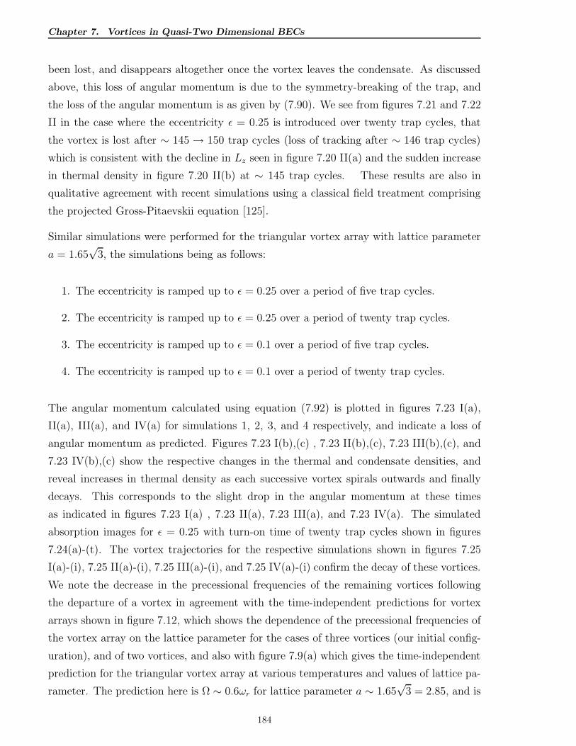
Chapter 7. Vortices in Quasi-Two Dimensional BECs
been lost, and disappears altogether once the vortex leaves the condensate. As discussed
above, this loss of angular momentum is due to the symmetry-breaking of the trap, and
the loss of the angular momentum is as given by (7.90). We see from figures 7.21 and 7.22
II in the case where the eccentricity ǫ = 0.25 is introduced over twenty trap cycles, that
the vortex is lost after ∼ 145 → 150 trap cycles (loss of tracking after ∼ 146 trap cycles)
which is consistent with the decline in Lz seen in figure 7.20 II(a) and the sudden increase
in thermal density in figure 7.20 II(b) at ∼ 145 trap cycles. These results are also in
qualitative agreement with recent simulations using a classical field treatment comprising
the projected Gross-Pitaevskii equation [125].
Similar simulations were performed for the triangular vortex array with lattice parameter
a = 1.65√
3, the simulations being as follows:
1. The eccentricity is ramped up to ǫ = 0.25 over a period of five trap cycles.
2. The eccentricity is ramped up to ǫ = 0.25 over a period of twenty trap cycles.
3. The eccentricity is ramped up to ǫ = 0.1 over a period of five trap cycles.
4. The eccentricity is ramped up to ǫ = 0.1 over a period of twenty trap cycles.
The angular momentum calculated using equation (7.92) is plotted in figures 7.23 I(a),
II(a), III(a), and IV(a) for simulations 1, 2, 3, and 4 respectively, and indicate a loss of
angular momentum as predicted. Figures 7.23 I(b),(c) , 7.23 II(b),(c), 7.23 III(b),(c), and
7.23 IV(b),(c) show the respective changes in the thermal and condensate densities, and
reveal increases in thermal density as each successive vortex spirals outwards and finally
decays. This corresponds to the slight drop in the angular momentum at these times
as indicated in figures 7.23 I(a) , 7.23 II(a), 7.23 III(a), and 7.23 IV(a). The simulated
absorption images for ǫ = 0.25 with turn-on time of twenty trap cycles shown in figures
7.24(a)-(t). The vortex trajectories for the respective simulations shown in figures 7.25
I(a)-(i), 7.25 II(a)-(i), 7.25 III(a)-(i), and 7.25 IV(a)-(i) confirm the decay of these vortices.
We note the decrease in the precessional frequencies of the remaining vortices following
the departure of a vortex in agreement with the time-independent predictions for vortex
arrays shown in figure 7.12, which shows the dependence of the precessional frequencies of
the vortex array on the lattice parameter for the cases of three vortices (our initial config-
uration), and of two vortices, and also with figure 7.9(a) which gives the time-independent
prediction for the triangular vortex array at various temperatures and values of lattice pa-
rameter. The prediction here is Ω ∼ 0.6ωr for lattice parameter a ∼ 1.65√
3 = 2.85, and is
184
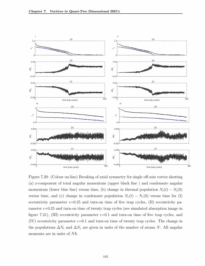
Chapter 7. Vortices in Quasi-Two Dimensional BECs
0
1.2
L z
I(a)
−0.01
0.03
∆Nt
(b)
0 300−0.03
0.01
time (trap cycles)
∆Nc
(c)
0
1.2
L z
(a)II
−0.01
0.03
∆Nt
(b)
0 300−0.03
0.01
time (trap cycles)
∆Nc
(c)
0.5
1
L z
III(a)
−0.001
0.004
∆Nt
(b)
0 300−0.004
0.001
time (trap cycles)
∆Nc
(c)
0.5
1
L z
IV(a)
−0.001
0.004
∆Nt
(b)
0 300−0.004
0.001
time (trap cycles)
∆Nc
(c)
Figure 7.20: (Colour on-line) Breaking of axial symmetry for single off-axis vortex showing
(a) z-component of total angular momentum (upper black line ) and condensate angular
momentum (lower blue line) versus time, (b) change in thermal population Nt(t)− Nt(0)
versus time, and (c) change in condensate population Nc(t) − Nc(0) versus time for (I)
eccentricity parameter ǫ=0.25 and turn-on time of five trap cycles, (II) eccentricity pa-
rameter ǫ=0.25 and turn-on time of twenty trap cycles (see simulated absorption image in
figure 7.21), (III) eccentricity parameter ǫ=0.1 and turn-on time of five trap cycles, and
(IV) eccentricity parameter ǫ=0.1 and turn-on time of twenty trap cycles. The change in
the populations ∆Nt and ∆Nc are given in units of the number of atoms N . All angular
momenta are in units of N~.
185
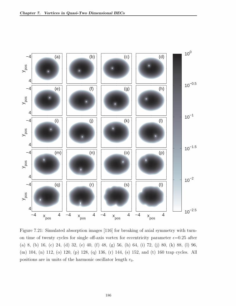
Chapter 7. Vortices in Quasi-Two Dimensional BECs
y pos
(a)−4
4
(b) (c) (d)
y pos
(e)−4
4
(f) (g) (h)
y pos
(i)−4
4
(j) (k) (l)
y pos
(m)−4
4
(n) (o) (p)
xpos
y pos
(q)
−4 4
−4
4
xpos
(r)
−4 4 xpos
(s)
−4 4 xpos
(t)
100
10−0.5
10−1
10−1.5
10−2
10−2.5
−4 4
Figure 7.21: Simulated absorption images [116] for breaking of axial symmetry with turn-
on time of twenty cycles for single off-axis vortex for eccentricity parameter ǫ=0.25 after
(a) 8, (b) 16, (c) 24, (d) 32, (e) 40, (f) 48, (g) 56, (h) 64, (i) 72, (j) 80, (k) 88, (l) 96,
(m) 104, (n) 112, (o) 120, (p) 128, (q) 136, (r) 144, (s) 152, and (t) 160 trap cycles. All
positions are in units of the harmonic oscillator length r0.
186
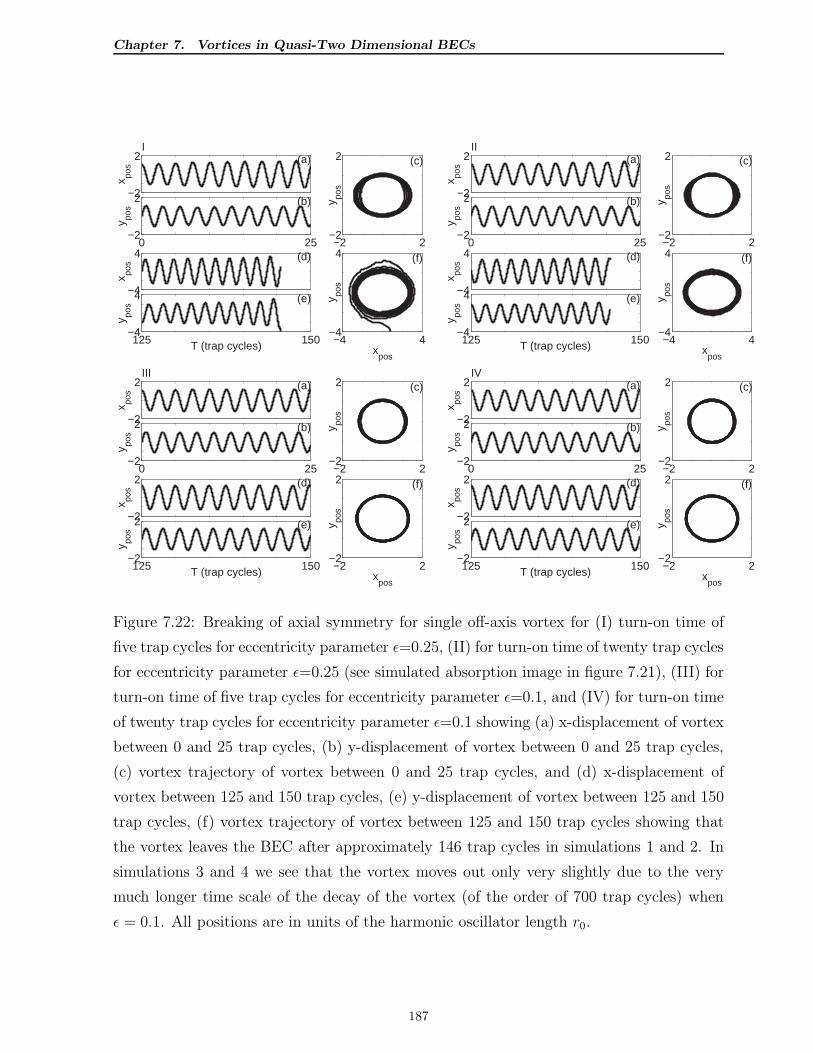
Chapter 7. Vortices in Quasi-Two Dimensional BECs
−2
2
x pos
I(a)
0 25−2
2
y pos
(b)
−4
4
x pos
(d)
125 150−4
4
T (trap cycles)
y pos
(e)
−2 2−2
2
y pos
(c)
−4 4−4
4
xpos
y pos
(f)
−2
2
x pos
II(a)
0 25−2
2
y pos
(b)
−4
4
x pos
(d)
125 150−4
4
T (trap cycles)
y pos
(e)
−2 2−2
2
y pos
(c)
−4 4−4
4
xpos
y pos
(f)
−2
2
x pos
III(a)
0 25−2
2
y pos
(b)
−2
2
x pos
(d)
125 150−2
2
T (trap cycles)
y pos
(e)
−2 2−2
2
y pos
(c)
−2 2−2
2
xpos
y pos
(f)
−2
2
x pos
IV(a)
0 25−2
2
y pos
(b)
−2
2
x pos
(d)
125 150−2
2
T (trap cycles)
y pos
(e)
−2 2−2
2
y pos
(c)
−2 2−2
2
xpos
y pos
(f)
Figure 7.22: Breaking of axial symmetry for single off-axis vortex for (I) turn-on time of
five trap cycles for eccentricity parameter ǫ=0.25, (II) for turn-on time of twenty trap cycles
for eccentricity parameter ǫ=0.25 (see simulated absorption image in figure 7.21), (III) for
turn-on time of five trap cycles for eccentricity parameter ǫ=0.1, and (IV) for turn-on time
of twenty trap cycles for eccentricity parameter ǫ=0.1 showing (a) x-displacement of vortex
between 0 and 25 trap cycles, (b) y-displacement of vortex between 0 and 25 trap cycles,
(c) vortex trajectory of vortex between 0 and 25 trap cycles, and (d) x-displacement of
vortex between 125 and 150 trap cycles, (e) y-displacement of vortex between 125 and 150
trap cycles, (f) vortex trajectory of vortex between 125 and 150 trap cycles showing that
the vortex leaves the BEC after approximately 146 trap cycles in simulations 1 and 2. In
simulations 3 and 4 we see that the vortex moves out only very slightly due to the very
much longer time scale of the decay of the vortex (of the order of 700 trap cycles) when
ǫ = 0.1. All positions are in units of the harmonic oscillator length r0.
187
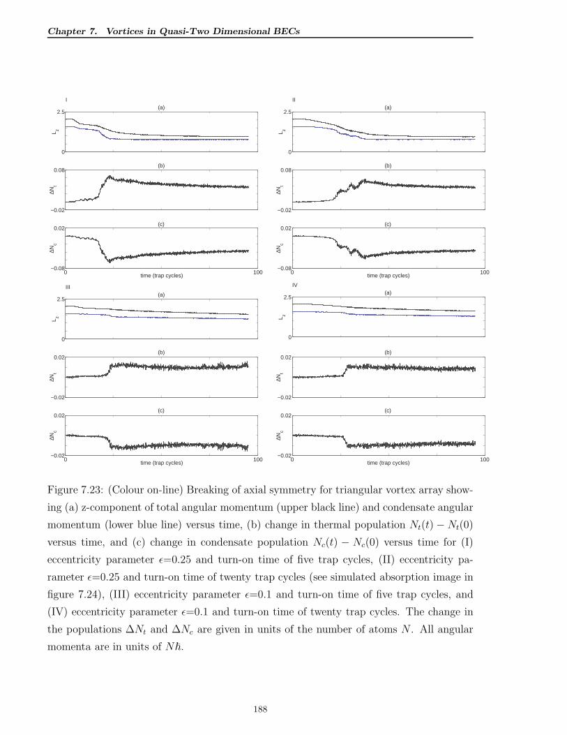
Chapter 7. Vortices in Quasi-Two Dimensional BECs
0
2.5
L z
I(a)
−0.02
0.08
∆Nt
(b)
0 100−0.08
0.02
time (trap cycles)
∆Nc
(c)
0
2.5
L z
II(a)
−0.02
0.08
∆Nt
(b)
0 100−0.08
0.02
time (trap cycles)∆N
c
(c)
0
2.5
L z
III(a)
−0.02
0.02
∆Nt
(b)
0 100−0.02
0.02
time (trap cycles)
∆Nc
(c)
0
2.5
L zIV
(a)
−0.02
0.02
∆Nt
(b)
0 100−0.02
0.02
time (trap cycles)
∆Nc
(c)
Figure 7.23: (Colour on-line) Breaking of axial symmetry for triangular vortex array show-
ing (a) z-component of total angular momentum (upper black line) and condensate angular
momentum (lower blue line) versus time, (b) change in thermal population Nt(t)− Nt(0)
versus time, and (c) change in condensate population Nc(t) − Nc(0) versus time for (I)
eccentricity parameter ǫ=0.25 and turn-on time of five trap cycles, (II) eccentricity pa-
rameter ǫ=0.25 and turn-on time of twenty trap cycles (see simulated absorption image in
figure 7.24), (III) eccentricity parameter ǫ=0.1 and turn-on time of five trap cycles, and
(IV) eccentricity parameter ǫ=0.1 and turn-on time of twenty trap cycles. The change in
the populations ∆Nt and ∆Nc are given in units of the number of atoms N . All angular
momenta are in units of N~.
188
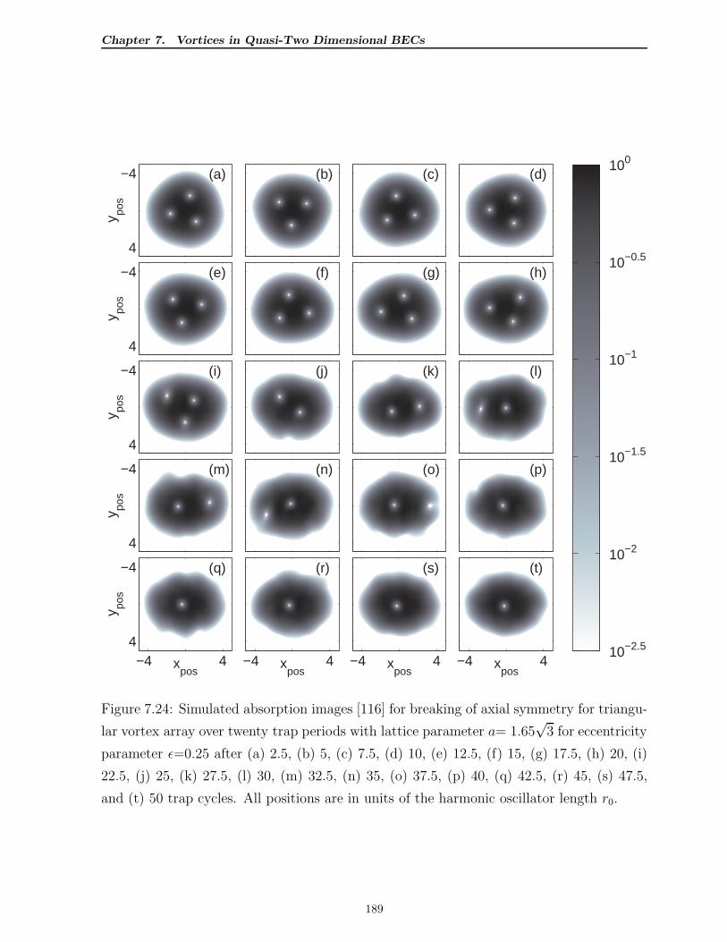
Chapter 7. Vortices in Quasi-Two Dimensional BECs
y pos
(a)−4
4
(b) (c) (d)
y pos
(e)−4
4
(f) (g) (h)
y pos
(i)−4
4
(j) (k) (l)
y pos
(m)−4
4
(n) (o) (p)
xpos
y pos
(q)
−4 4
−4
4
xpos
(r)
−4 4 xpos
(s)
−4 4 xpos
(t)
100
10−0.5
10−1
10−1.5
10−2
10−2.5
−4 4
Figure 7.24: Simulated absorption images [116] for breaking of axial symmetry for triangu-
lar vortex array over twenty trap periods with lattice parameter a= 1.65√
3 for eccentricity
parameter ǫ=0.25 after (a) 2.5, (b) 5, (c) 7.5, (d) 10, (e) 12.5, (f) 15, (g) 17.5, (h) 20, (i)
22.5, (j) 25, (k) 27.5, (l) 30, (m) 32.5, (n) 35, (o) 37.5, (p) 40, (q) 42.5, (r) 45, (s) 47.5,
and (t) 50 trap cycles. All positions are in units of the harmonic oscillator length r0.
189
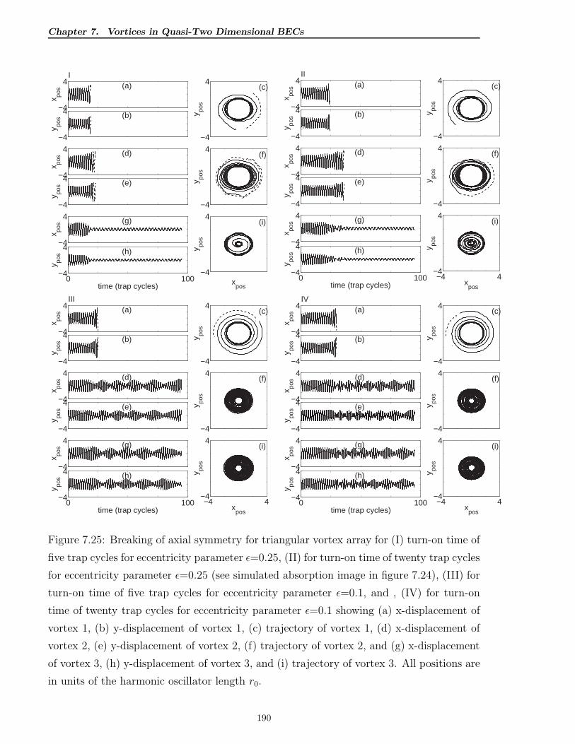
Chapter 7. Vortices in Quasi-Two Dimensional BECs
−4
4
x pos
I(a)
−4
4
y pos (b)
−4
4
x pos (d)
−4
4
y pos (e)
−4
4
x pos (g)
0 100−4
4
time (trap cycles)
y pos (h)
−4
4
y pos
(c)
−4
4
y pos
(f)
−4
4
xpos
y pos
(i)
−4
4
x pos
II(a)
−4
4
y pos (b)
−4
4
x pos (d)
−4
4
y pos (e)
−4
4
x pos (g)
0 100−4
4
time (trap cycles)y po
s (h)
−4
4
y pos
(c)
−4
4
y pos
(f)
−4 4−4
4
xpos
y pos
(i)
−4
4
x pos
III(a)
−4
4
y pos (b)
−4
4
x pos (d)
−4
4
y pos (e)
−4
4
x pos (g)
0 100−4
4
time (trap cycles)
y pos (h)
−4
4
y pos
(c)
−4
4
y pos
(f)
−4 4−4
4
xpos
y pos
(i)
−4
4
x pos
IV(a)
−4
4
y pos (b)
−4
4
x pos (d)
−4
4
y pos (e)
−4
4
x pos (g)
0 100−4
4
time (trap cycles)
y pos (h)
−4
4
y pos
(c)
−4
4
y pos
(f)
−4 4−4
4
xpos
y pos
(i)
Figure 7.25: Breaking of axial symmetry for triangular vortex array for (I) turn-on time of
five trap cycles for eccentricity parameter ǫ=0.25, (II) for turn-on time of twenty trap cycles
for eccentricity parameter ǫ=0.25 (see simulated absorption image in figure 7.24), (III) for
turn-on time of five trap cycles for eccentricity parameter ǫ=0.1, and , (IV) for turn-on
time of twenty trap cycles for eccentricity parameter ǫ=0.1 showing (a) x-displacement of
vortex 1, (b) y-displacement of vortex 1, (c) trajectory of vortex 1, (d) x-displacement of
vortex 2, (e) y-displacement of vortex 2, (f) trajectory of vortex 2, and (g) x-displacement
of vortex 3, (h) y-displacement of vortex 3, and (i) trajectory of vortex 3. All positions are
in units of the harmonic oscillator length r0.
190
Chapter 7. Vortices in Quasi-Two Dimensional BECs
in good agreement with the time-dependent value estimated using a least-squares method
of a slowly-varying sinusoid to the vortex x-displacement versus time (see figure 7.25 for
xpos versus T and ypos versus T ). We also see good agreement with the value of the preces-
sional frequencies of a single vortex (after the other two vortices have left the condensate)
indicated in figure 7.25 again estimated using a least-squares method of a slowly-varying
sinusoid to the vortex x-displacement versus time, and the time-independent predictions
given in figure 7.5(a). We note that the simulation absorption images in figures 7.24 and
the vortex trajectory diagrams in 7.25 II which show the vortex decay for the case where
the eccentricity ǫ = 0.25 is introduced over 20 trap cycles are consistent, indicating a decay
time of ∼ 24 trap cycles for the first vortex, and a decay time of ∼ 38 trap cycles for the
second. This is also consistent with figure 7.23 II which shows sudden changes in thermal
density at these times, and a steady decrease in Lz with slight drops accompanying the
decay of each vortex. We also note a sudden change in the thermal density after ∼ 30 trap
cycles. This accompanies the complex precessional motion of the third vortex at ∼ 30 trap
cycles as shown in figures 7.25 II(g),(h) due to the interaction between the vortices. The
lifetimes of the vortices in the case of the triangular vortex for ǫ = 0.25 varies considerably
- the first vortex to leave the condensate has a lifetime of between ∼ 20 and ∼ 25 trap
cycles, while the second has a lifetime varying between ∼ 25 and ∼ 38 depending on the
scenario - see figures 7.23 I(a)-(c) and 7.23 II(a)-(c). In all cases the loss of a vortex is
characterised by a slight drop in Lz and sudden increases in the thermal population with
a corresponding drop in the condensate population (see figure 7.23). The departure of the
vortices is also marked by the trajectories of the vortices shown in figures 7.25 I(a)-(f) and
7.25 II(a)-(f) where we see the end of the vortex tracks. The lifetime of the remaining
vortex can only be inferred from figures 7.23 I(a) and 7.23 II(a) by extrapolation, and is
of the order of 300-400 trap cycles (since the residual angular momentum (i.e. the angular
momentum at the time that only a single vortex remains) is higher than in the single
vortex case). In the case of the triangular vortex array for ǫ = 0.1, the lifetime of the first
vortex is of the same order (∼ 25 → 30 trap cycles), but the lifetimes for the second and
third vortices are considerably longer, the second vortex having an extrapolated lifetime
of ∼ 400 trap cycles (see figures 7.23 III and 7.23 IV). It is impossible to ascertain the
lifetime of the remaining vortex from the simulations, but it is probably of the order of a
few thousand trap cycles which is impractical to simulate with the facilities available.
191
Chapter 7. Vortices in Quasi-Two Dimensional BECs
7.6 Conclusions
By solving the orthogonal HFB equations in the frame rotating at the precessional fre-
quency of the vortex predicted using the continuity equation for the condensate, and solv-
ing this self-consistently with the orthogonal HFB equations, we were able to predict the
precessional frequency of off-axis vortices in BECs for given values of a (the distance of the
vortex from the axis) and T (the temperature of the BEC). In these calculations, the vor-
tex position is specified in the modified basis functions for the condensate wave-function.
The precessional frequencies and LCLS energies for on-axis vortices were determined by
extrapolation, and the LCLS energies found to be consistent with on-axis solutions to the
orthogonal HFB equations for BECs having a single vortex rotating at the extrapolated
precessional frequency. In this way we were able to demonstrate that there is no correlation
between the LCLS energies and the precessional frequencies of off-axis vortices (contrary
to that which was previously believed). We also established a correspondence between this
formulation and a generalised multi-state model. These results are consistent with GPE
simulations, and are also in qualitative agreement with the projected GPE simulations.
We were able to generalise this technique to vortex arrays, and thus were able to produce
plots of the precessional frequencies of these vortex arrays as a function of lattice param-
eter a and temperature T . We also obtained qualitative agreement with the areal density
approximation for the hexagonal vortex array.
These predictions were verified using time-dependent simulations in both the cases of the
single off-axis vortex and of vortex arrays consisting of two, three and seven vortices. Sim-
ulations of a BEC stirred with one or three narrow-beam Gaussian stirrers also produced
vortices precessing at frequencies in agreement with these predictions. In these simulations
a critical stirring frequency about 10-20% in excess of the local Landau critical velocity for
the creation of vortices within the Thomas-Fermi radius was found, and this is consistent
with the notion already expressed that the critical velocity is increased by the presence of
the energy gap in the HFB spectrum, and the fact that the HFB spectrum is steepened
with respect to the Bogoliubov spectrum by the presence of the anomalous density.
Finally we showed that breaking the axial symmetry of the trapping potential leads to
loss of angular momentum of the BEC, and hence to vortex decay. We demonstrated
this for both off-axis vortices, and for triangular vortex arrays by the introduction of an
eccentricity ǫ into the trapping potential, and were able to establish approximate life-times
for the vortices in both cases for ǫ = 0.25, and ǫ = 0.1.
192
Chapter 8. Finite Temperature Mean Field Theory for 1D Optical Lattice
Chapter 8
Finite Temperature Mean Field
Theory for 1D Optical Lattice
8.1 Introduction
Ultracold atoms confined within optical potentials [126] are of great current interest, both
theoretically [127–140] and experimentally [141,142]. Optical lattices can be generated with
extraordinary levels of control and used to simulate more complicated, less perfect and,
often, less manipulable condensed-matter systems [143–146]. Ultracold atoms in optical
lattices have also been proposed as candidates for quantum information processing [147],
with applications in quantum cryptography and quantum computing. Various methods of
loading and manipulating Bose-Einstein condensates in optical lattices have been proposed
[148–152] and this is now routinely performed.
We consider a quasi-one-dimensional gas with tight radial confinement such that only
axial degrees of freedom are available, but where the scattering is still effectively three-
dimensional [153,154]. We then impose a one-dimensional optical lattice in the axial direc-
tion. We extend previous treatments at zero temperature [128, 129] to finite temperature
using the Hartree-Fock-Bogoliubov mean-field treatment as applied to a discrete Bose-
Hubbard model, yielding modified Gross-Pitaevskii and Bogoliubov de Gennes equations.
This set of equations is solved for both the case of a translationally invariant lattice (no
external trapping potential) and an inhomogeneous lattice (optical lattice in an external
harmonic trapping potential). The use of the mean-field based treatment means we can
only consider the superfluid phase for the atoms in the optical lattice. The model is not
193
Chapter 8. Finite Temperature Mean Field Theory for 1D Optical Lattice
valid in the Mott insulator regime. We use the model to estimate the superfluid to normal
phase-transition temperature in each case. We are then able to obtain a phase diagram for
the superfluid and normal gas states in the low effective interaction strength limit. We note
that Kleinert et. al. [155] have considered a homogeneous three-dimensional optical lattice
(untrapped case) and predict an upward shift in the critical temperature which reduces
once more for large effective interaction strengths to give re-entrant-type behaviour1. This
is consistent with our findings for the one-dimensional system.
8.2 The Hartree-Fock Bogoliubov Treatment of a Bose
Einstein Condensate in a one-dimensional Optical
Lattice in the Popov Approximation
Let us consider a one-dimensional optical lattice with I lattice sites. If one expands the
Bose field operators in the Wannier basis and applies the tight-binding approximation,
one obtains the Bose-Hubbard model. The Bose-Hubbard Hamiltonian for atoms in a
one-dimensional optical lattice may be written in the form [127–129]
H =I∑
i=1
niǫi − JI∑
i=1
(
a†i+1ai + a†i ai+1
)
+V
2
I∑
i=1
ni (ni − 1) (8.1)
where J represents the coupling strength between adjacent lattice sites, V is the interaction
potential acting between atoms on the same site, and ai is the Bose field operator for the
ith lattice site, and ni = a†i ai . ǫi is the non-interacting energy of the atoms on each site i.
The usual commutation relations apply for the Bose field operator ai, ie.
[
aj , a†k
]
= δj,k , [aj , ak] =[
a†j, a†k
]
= 0. (8.2)
Assuming a macroscopic occupation of the ground state, we express the Bose annihilation
operator for each lattice site i in terms of a complex part zi and a fluctuation operator
part δi as follows [128,129]:
ai =(
zi + δi
)
exp
(−iµt~
)
. (8.3)
1The phase diagram in figure 1 [155] (effective scattering length aeff/a(0)eff versus the temperature
T/T(0)c ) exhibits a re-entrant transition above the critical temperature T
(0)c of the free system, i.e. the
transition curve has a nose. This implies that for T > T(0)c it is possible to create a condensate by increasing
aeff which then disappears when aeff is increased further.
194
Chapter 8. Finite Temperature Mean Field Theory for 1D Optical Lattice
We substitute equation (8.3) into the Hamiltonian (8.1) and take the self-consistent mean-
field approximation such that δ†i δiδi → 2⟨
δ†i δi
⟩
δi +⟨
δiδi
⟩
δi,⟨
δi
⟩
=⟨
δ†i
⟩
= 0, zi = 〈zi〉,
δ†i δi →⟨
δ†i δi
⟩
= ni and δiδi →⟨
δiδi
⟩
= mi, where nci= |zi|2 is the density of the
condensate atoms, ni =⟨
δ†i δi
⟩
is the excited population density, mi =⟨
δiδi
⟩
is the
anomalous density (which we ignore in the Popov approximation), ni = nci+ ni is the
overall number density (ie. the sum of the condensate and excitation population number
densities), and where mi = z2i + mi.
The resulting Hamiltonian can now be diagonalised provided the fluctuations δi satisfy the
Bogoliubov (canonical) transformation
δi =∑
q
[
uqi αqe
−iωqt − vq∗
i α†qe
iωqt]
(8.4)
with Hermitian conjugate
δ†i =∑
q
[
uq∗
i α†qe
iωqt − vqi αqe
−iωqt]
(8.5)
where uqi and vq
i are the quasiparticle amplitudes, ωq are the quasiparticle excitation fre-
quencies, α†q is the quasiparticle creator operator, and αq the quasiparticle destructor op-
erator.
Finally one obtains (for details see [128,129]) the set of coupled equations (in dimensionless
form) comprising the modified Gross-Pitaevskii equation
µ′zi = ǫ′izi − (zi+1 + zi−1) + Veff (ncizi + 2nizi) (8.6)
and the Bogoliubov-de Gennes equations
ǫq′
uqi + c′qzi = [2Veff (nci
+ ni)− µ′ + ǫ′i] uqi −
[
uqi+1 + uq
i−1
]
− Veffz2i v
qi
−ǫq′vqi − c′qzi = [2Veff (nci
+ ni)− µ′ + ǫ′i] vqi −
[
vqi+1 + vq
i−1
]
− Veffz2i u
qi
(8.7)
with
ni =⟨
δ†i δi
⟩
=∑
q
[
|vqi |
2+(
|uqi |
2+ |vq
i |2)
NBE
(
ǫq′)]
(8.8)
where
NBE
(
ǫq′)
=1
Z−1eβǫq′ − 1(8.9)
is the usual Bose distribution and Veff = V/J , µ′ = µ/J , ǫq′
= ǫq/J = ~ωq/J , ǫ′i = ǫi/J ,
J = ~2/2ma2, and where we have assumed without loss of generality the condensate am-
plitudes zi to be real (which they are to an arbitrary phase constant). µ is the energy
195
Chapter 8. Finite Temperature Mean Field Theory for 1D Optical Lattice
eigenvalue for the modified Gross-Pitaevskii equation (and approximates the chemical po-
tential closely for values of temperature well below the transition temperature), ǫq is the
energy eigenvalue of the Bogoliubov-de Gennes equations, and ǫi is the value of the trap-
ping potential at site i. The cq’s are necessary in order to ensure the orthogonality of the
condensate with the excited states [23, 24, 156] and are given by
cq =V
N0
∑
|zj |2(
z∗juqj − zjv
qj
)
. (8.10)
Z is a fugacity term resulting from the difference between the true chemical potential µT ,
and the chemical potential as estimated using the eigenvalue µ corresponding to the ground
state of the modified Gross-Pitaevskii equation (equation (8.6)). Thus
Z = exp (β (µT − µ)) (8.11)
where β = 1/kBT is the temperature parameter, with kB Boltzmann’s constant and T the
temperature. Equation (8.8) follows in view of the fact that 〈aqaq′〉 =⟨
a†qa†q′
⟩
= 0 and⟨
a†qaq′⟩
= NBE(ǫq)δqq′.
In the case of a homogeneous gas having a large number of particles in the ground state
(ie. nc ≫ 1), the fugacity may be approximated by [23, 24]
Z = 1 + 1/nc. (8.12)
In these calculations we neglect these finite-size effects, which are only significant near the
transition temperature Tc and take the fugacity Z to be unity.
We also require that the total number of atoms satisfy the condition [129]
N =I∑
i=1
[nci+ ni] =
I∑
i=1
[
|zi|2 + ni
]
= nc + n. (8.13)
The condensate fraction is simply
fc =nc
nc + n=nc
N=
∑Ii=1 nci
N=
∑Ii=1 |zi|2N
. (8.14)
Superfluid flow of the condensate occurs when there is a phase gradient. A phase gradient of
the condensate modifies the hopping term of the Hamiltonian by the introduction of Peierls
phase factors e±i∆φ where ∆φ is the phase factor between ai and ai+1. The resulting energy
shift may be estimated using second order perturbation theory. Since this energy shift is
due entirely to the kinetic energy associated with the superfluid flow, and hence due to the
196
Chapter 8. Finite Temperature Mean Field Theory for 1D Optical Lattice
superfluid fraction, it follows that the superfluid fraction fs may be calculated in terms of
this energy shift. It turns out that [128, 129]
fs =1
N
Eφ − E0
J (∆φ)2 = − 1
2NJ〈ψ0| T |ψ0〉 −
1
NJ
∑
ν 6=0
∣
∣
∣〈ψν | J |ψν〉
∣
∣
∣
2
Eν − E0= f (1)
s − f (2)s (8.15)
where we have defined the operators
J ≡ iJ
I∑
i=1
(
a†i+1ai − a†i ai+1
)
and
T ≡ JI∑
i=1
(
a†i+1ai + a†i ai+1
)
,
and where E0 and Eν are the energies corresponding respectively to the ground state |ψ0〉and the excited state |ψν〉 , ν = 1, 2, .... Finally, we obtain the following expression for the
superfluid fraction fS in terms of the condensate and quasiparticle amplitudes [128, 129]:
fs = f (1)s − f (2)
s (8.16)
where
f (1)s =
1
2N
I∑
i=1
[
(
zi+1z∗i + z∗i+1zi
)
+∑
q
(
vqi v
q∗
i+1 + vq∗
i vqi+1
)
]
(8.17)
and
f (2)s =
J
N
∑
q,q′
∣
∣
∣
∑
i
(
uqi+1v
q′
i − uqiv
q′
i+1
)∣
∣
∣
2
~ωq + ~ωq′+ δqq′
∣
∣
∑
i
(
uqi+1v
qi − uq
ivqi+1
)∣
∣
2
2~ωq
. (8.18)
8.3 Translationally Invariant Lattice
In the case of a translationally invariant lattice, periodic boundary conditions apply, and
the quasi-particle amplitudes are given by
uqj =
uqei(qja)
√I
, vqj =
vqei(qja)
√I
, 1 ≤ j ≤ I − 1. (8.19)
Furthermore the condensate amplitudes are equal for each site j, thus zj = z, ncj= |zj |2 =
|z|2 = z2 = nc for 1 ≤ j ≤ I−1 since z has been taken without loss of generality to be real.
Since there is no trapping potential, ǫi = ǫ = 0 for 1 ≤ j ≤ I − 1. For the translationally
invariant lattice
µ =
(
|z|2I
+ 2n
)
V − 2J (8.20)
197
Chapter 8. Finite Temperature Mean Field Theory for 1D Optical Lattice
where
n =1
I
∑
q
[
|vq|2 +(
|uq|2 + |vq|2)
NBE (ǫq)]
(8.21)
is the thermal population. Noting that cq = 0 for the case of a translationally invariant
lattice, it can be shown that for the translationally invariant lattice [129]
|uq|2 =V z2 + 4J sin2
(
qa2
)
+ ~ωq
2~ωq, (8.22)
|vq|2 =V z2 + 4J sin2
(
qa2
)
− ~ωq
2~ωq, (8.23)
and
ǫq = ~ωq =√
K(q) [2ncV +K(q)], (8.24)
where
K(q) = 4J sin2(qa
2
)
. (8.25)
Thus from equations (8.16), (8.17) and (8.18), for the translationally invariant lattice, the
superfluid fraction is given by
fs =1
N
(
I |z|2 +I−1∑
j=1
|vq|2 cos
(
2πj
I
)
)
(8.26)
since q = 2πj/Ia for 1 ≤ j ≤ I − 1.
The condensate fraction for a given lattice site is given by fc = nc/n0 where n0 = N/I is the
number of atoms per site. By equations (8.13) and (8.14), we have for the translationally
invariant lattice,
N = I |z|2 + n = I |z|2 +
I−1∑
j=1
[
∣
∣v(j)∣
∣
2+(
∣
∣u(j)∣
∣
2+∣
∣v(j)∣
∣
2)
NBE
(
ǫ(j))
]
. (8.27)
To calculate the condensate and superfluid fraction for the translationally invariant lattice,
we first determine the condensate amplitude. Then writing
gj(n) = |z|2(n−1) Veff + 4 sin2
(
πj
I
)
, (8.28)
ej(n) = 2 sin
(
πj
I
)
√
2 |z|2(n−1) Veff + 4 sin2
(
πj
I
)
(8.29)
and
NBEj(n)=
1
exp(
β ′ej(n−1)
)
− 1(8.30)
198
Chapter 8. Finite Temperature Mean Field Theory for 1D Optical Lattice
where β ′ = Jβ = J/kBT = 1/keffT , with keff = kB/J , and where the subscript (n) refers
to the variable in question at the nth iteration, one can solve for |z|2 using the iterative
scheme
|z|2(n) =1
I
(
N −I−1∑
j=1
[
gj(n) − ej(n)
2ej(n)
+gj(n)
ej(n)
NBEj(n)
]
)
. (8.31)
As an initial guess, the value |z|2(n) = NI
is used, and the calculations (8.28), (8.29), (8.30)
and (8.31) repeated until convergence is attained (ie.∣
∣
∣|z|2(n) − |z|
2(n−1)
∣
∣
∣< Error Tolerance),
or the maximum number of iterations is exceeded (divergent solution)).
One first calculates gj(n), ej(n) and NBEj(n)using equations (8.28), (8.29) and (8.30). The
quasiparticle amplitudes (given by equations (8.19)) may be calculated using the equations
∣
∣u(j)∣
∣
2
(n)=gj(n) + ej(n)
2ej(n)
(8.32)
and∣
∣v(j)∣
∣
2
(n)=gj(n) − ej(n)
2ej(n)
. (8.33)
The condensate and superfluid fractions are then readily determined.
8.4 Inhomogeneous Lattice
The condensate amplitudes zi are found by solving equation (8.6) where the trapping
potential is given by ǫi = Ω [i− (I + 1) /2]2 for site i with Ω = 12mω2a2, and a is the inter-
lattice spacing. The quasi-particle amplitudes for site i, uqi and vq
i are found by solving
equations (8.7).
This set of equations can again be solved iteratively. In performing this calculation, we
actually set the cq′
s to zero when solving the Bogoliubov-de Gennes equations, but do
so in the GGPE basis, thus ensuring orthogonality of the ground state and the excited
states [23, 24]. The GGPE basis is given by the normalised solutions to the eigenvalue
problem given by equation (8.6), with the ground state (zero energy solution) excluded.
Let us rewrite the Bogoliubov-de Gennes equations (8.7) in matrix form
ǫq
[
uq
vq
]
=
[
L M
−M −L
][
uq
vq
]
(8.34)
199
Chapter 8. Finite Temperature Mean Field Theory for 1D Optical Lattice
where
uq =
uq−I...
uqi...
uqI
, vq =
vq−I...
vqi...
vqI
(8.35)
L = 2Veff (nci+ ni)− µ+ Ωi2 − J (8.36)
and
M = −Veffz2i . (8.37)
Here J is defined as the operator acting on zi, uqi , and vq
i as follows:
J uqi = uq
i+1 + uqi−1 (8.38)
for example. In deriving equation (8.6), we used the fact that we can take the condensate
amplitudes zi (without loss of generality) to be real.
Now, let zqi constitute the eigenstates of equation (8.6) with eigenvalues µq. We order
the normalised eigenvalues into ascending order, and order the eigenstates accordingly, call
these ξqi . The state ξ0
i corresponds to the Goldstone mode, we must exclude this in order
to obtain the GGPE basis. Let us define the matrix
U =[
ξ1 . . . ξq . . . ξ2I]
(8.39)
where
ξq =
ξq1...
ξqi...
ξq2I+1
. (8.40)
Let uqHFB,v
qHFB be the solution to the Bogoliubov-de Gennes equations in the GGPE
basis, then the solution to the matrix equation
ǫq
[
uqHFB
vqHFB
]
=
[
UT LU UTMU
−UTMU −UT LU
][
uqHFB
vqHFB
]
(8.41)
gives the Bogoliubov quasiparticle amplitudes in the GGPE basis. To obtain the Bogoli-
ubov quasiparticle amplitudes uqi , v
qi one transforms back using
uq = UuqHFB
vq = UvqHFB.
(8.42)
200
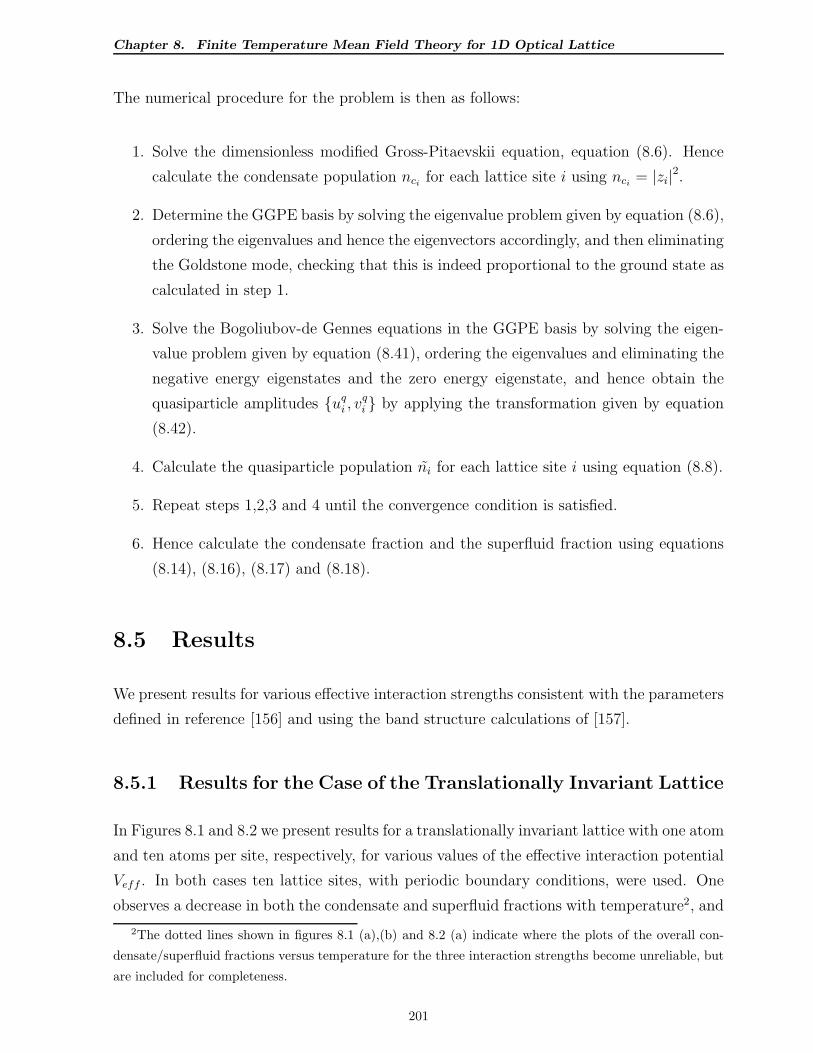
Chapter 8. Finite Temperature Mean Field Theory for 1D Optical Lattice
The numerical procedure for the problem is then as follows:
1. Solve the dimensionless modified Gross-Pitaevskii equation, equation (8.6). Hence
calculate the condensate population ncifor each lattice site i using nci
= |zi|2.
2. Determine the GGPE basis by solving the eigenvalue problem given by equation (8.6),
ordering the eigenvalues and hence the eigenvectors accordingly, and then eliminating
the Goldstone mode, checking that this is indeed proportional to the ground state as
calculated in step 1.
3. Solve the Bogoliubov-de Gennes equations in the GGPE basis by solving the eigen-
value problem given by equation (8.41), ordering the eigenvalues and eliminating the
negative energy eigenstates and the zero energy eigenstate, and hence obtain the
quasiparticle amplitudes uqi , v
qi by applying the transformation given by equation
(8.42).
4. Calculate the quasiparticle population ni for each lattice site i using equation (8.8).
5. Repeat steps 1,2,3 and 4 until the convergence condition is satisfied.
6. Hence calculate the condensate fraction and the superfluid fraction using equations
(8.14), (8.16), (8.17) and (8.18).
8.5 Results
We present results for various effective interaction strengths consistent with the parameters
defined in reference [156] and using the band structure calculations of [157].
8.5.1 Results for the Case of the Translationally Invariant Lattice
In Figures 8.1 and 8.2 we present results for a translationally invariant lattice with one atom
and ten atoms per site, respectively, for various values of the effective interaction potential
Veff . In both cases ten lattice sites, with periodic boundary conditions, were used. One
observes a decrease in both the condensate and superfluid fractions with temperature2, and
2The dotted lines shown in figures 8.1 (a),(b) and 8.2 (a) indicate where the plots of the overall con-
densate/superfluid fractions versus temperature for the three interaction strengths become unreliable, but
are included for completeness.
201
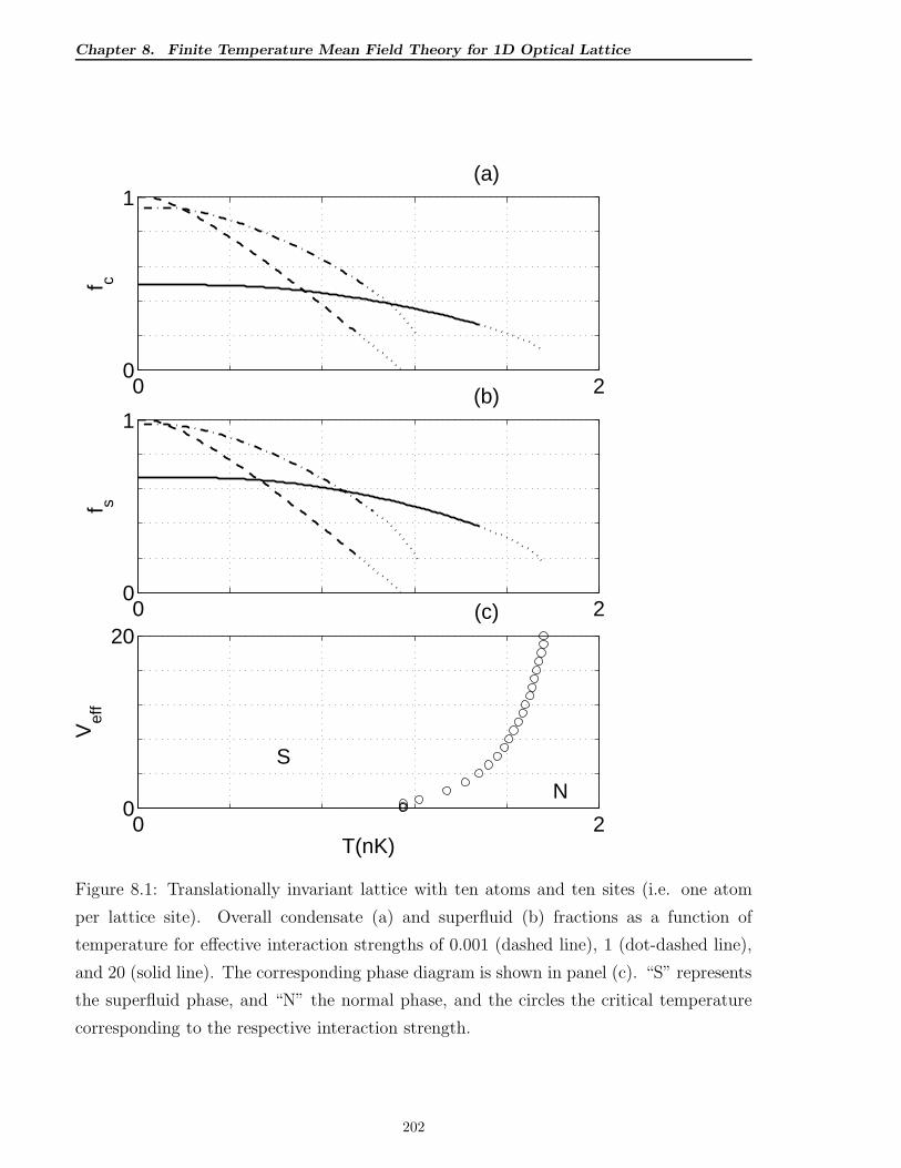
Chapter 8. Finite Temperature Mean Field Theory for 1D Optical Lattice
0 20
1 (a)
f c
0 20
1 (b)
f s
0 20
20
S
N
(c)
T(nK)
Vef
f
Figure 8.1: Translationally invariant lattice with ten atoms and ten sites (i.e. one atom
per lattice site). Overall condensate (a) and superfluid (b) fractions as a function of
temperature for effective interaction strengths of 0.001 (dashed line), 1 (dot-dashed line),
and 20 (solid line). The corresponding phase diagram is shown in panel (c). “S” represents
the superfluid phase, and “N” the normal phase, and the circles the critical temperature
corresponding to the respective interaction strength.
202
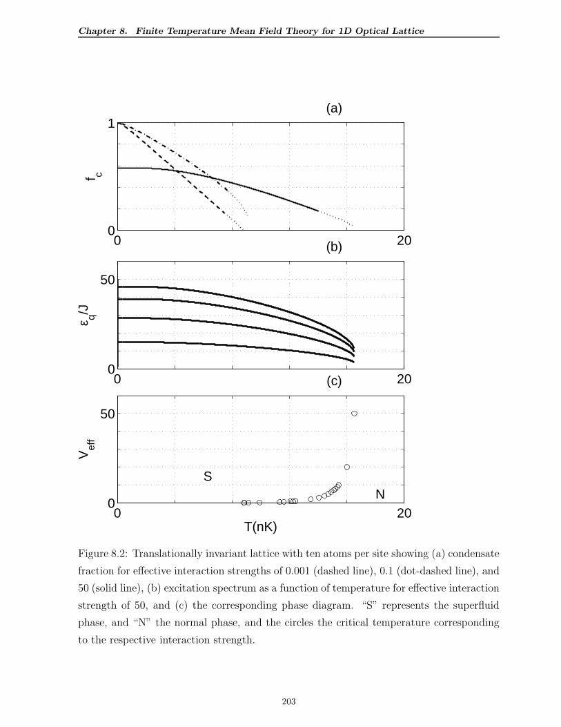
Chapter 8. Finite Temperature Mean Field Theory for 1D Optical Lattice
0 200
1 (a)
f c
0 200
50
(b)
ε q/J
0 200
50
SN
(c)
T(nK)
Vef
f
Figure 8.2: Translationally invariant lattice with ten atoms per site showing (a) condensate
fraction for effective interaction strengths of 0.001 (dashed line), 0.1 (dot-dashed line), and
50 (solid line), (b) excitation spectrum as a function of temperature for effective interaction
strength of 50, and (c) the corresponding phase diagram. “S” represents the superfluid
phase, and “N” the normal phase, and the circles the critical temperature corresponding
to the respective interaction strength.
203
Chapter 8. Finite Temperature Mean Field Theory for 1D Optical Lattice
we interpret the point at which these densities approach zero as indicative of the critical
temperature Tc for the superfluid to normal gas phase transition. Our calculations make
the assumption that the true chemical potential and the lowest energy eigenvalue for the
modified Gross-Pitaevskii equation are equal. This tends to underestimate the transition
temperature3, but should provide a useful criterion for the transition between superfluid
and normal behaviour4. This interpretation is supported by an examination of the low-
lying excitation spectrum5 which, for the case Veff = 50, is shown in panel (b) of figure
8.2. The “softening” of the modes, indicative of the phase transition, is clearly seen and
coincides with the transition temperature obtained by noting the temperature at which
the condensate and superfluid densities approach zero.
We obtain such a “transition”6 temperature for each value of the effective interaction
potential Veff , producing a phase diagram as shown in figures 8.1(c) and 8.2(c), where the
superfluid phase and the normal phase are as indicated, the superfluid phase lying to the
left of the curve. The transition to the Mott insulator phase cannot be accounted for by this
formalism, but would in practice occur when Veff = V/J exceeds some critical value. In all
instances, the critical temperature for the transition from superfluid to normal gas increases
with the effective interaction potential, as is indeed the case with a homogeneous Bose gas
(i.e. a Bose gas in the absence of an optical lattice and confining potential) [158,159]. This
behaviour has also been predicted by Kleinert et. al. [155]. Our results are consistent with
their conclusions. In addition, they predict a reduction of the critical temperature as the
effective interaction strength is increased further. We, however, are unable to explore this
regime for the one-dimensional lattice as it extends beyond the validity of our model.
8.5.2 Results for the Case of the Inhomogeneous Lattice
Figure 8.3 shows plots of the number of condensate atoms, excited atoms and of the to-
tal number of atoms for each lattice site for the case of an inhomogeneous optical lattice
3For an infinite, homogeneous one-dimensional lattice (no external trapping potential), the transition
temperature is zero, so no superfluid behaviour is ever possible. Here we are interested in the shift in
critical temperature due to the effect of interactions which we obtain by considering a finite system4Note that, in the Bose-Hubbard model, the condensate number approaches the filling factor as the
temperature tends to infinity, so the condensate and superfluid fractions are never strictly zero for the
finite size system.5The lines shown in figure 8.2 (b) represent the quasi-particle excitation energies q = 0, 1, 2, 3 in
ascending order.6We only see a “transition” because of the finite size of our system. There is, however, no transition in
the thermodynamic limit.
204
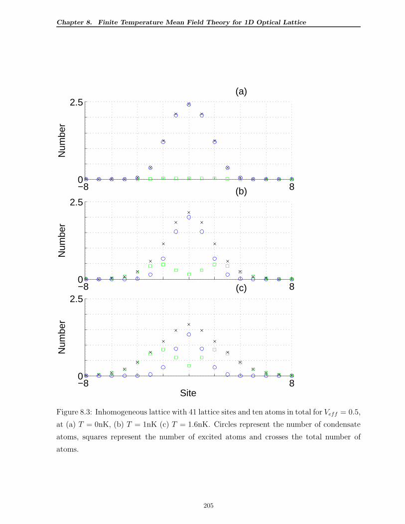
Chapter 8. Finite Temperature Mean Field Theory for 1D Optical Lattice
−8 80
2.5 (a)
Num
ber
−8 80
2.5 (b)
Num
ber
−8 80
2.5 (c)
Site
Num
ber
Figure 8.3: Inhomogeneous lattice with 41 lattice sites and ten atoms in total for Veff = 0.5,
at (a) T = 0nK, (b) T = 1nK (c) T = 1.6nK. Circles represent the number of condensate
atoms, squares represent the number of excited atoms and crosses the total number of
atoms.
205
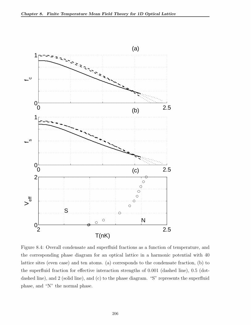
Chapter 8. Finite Temperature Mean Field Theory for 1D Optical Lattice
0 2.50
1 (a)
f c
0 2.50
1 (b)
f s
2 2.50
2
S
N
(c)
T(nK)
Vef
f
Figure 8.4: Overall condensate and superfluid fractions as a function of temperature, and
the corresponding phase diagram for an optical lattice in a harmonic potential with 40
lattice sites (even case) and ten atoms. (a) corresponds to the condensate fraction, (b) to
the superfluid fraction for effective interaction strengths of 0.001 (dashed line), 0.5 (dot-
dashed line), and 2 (solid line), and (c) to the phase diagram. “S” represents the superfluid
phase, and “N” the normal phase.
206
Chapter 8. Finite Temperature Mean Field Theory for 1D Optical Lattice
consisting of 41 lattice sites (odd case) with ten atoms in total. The plots are for Veff = 1
at various temperatures ranging from T = 0 to T = 1.6nK. At zero temperature, the
condensate atom distribution is bell-shaped, peaked at the central lattice site. There is a
small quantum depletion even at zero temperature, and the distribution of excited atoms
is shaped as a bimodal distribution, centred about the central lattice site. As the tem-
perature increases, the condensate population decreases, but the distribution still remains
bell-shaped, and the excited population increases. In figure 8.4 we present the overall con-
densate and superfluid fractions and the corresponding phase diagram for optical lattices
in a harmonic potential consisting of 40 lattice sites (even case). Panel (a) corresponds to
the condensate fraction, (b) the superfluid fraction, and (c) the phase diagram. The dotted
lines shown in panels (a) and (b) indicate where the plots of the overall condensate and
superfluid fractions versus temperature for the three interaction strengths become unreli-
able, but are included for completeness. We note that for higher temperatures, calculations
performed using 41 lattice sites begin to show a marked difference. This is indicative of
the fact that we are pushing the bounds of validity of our model. In particular we are
seeing significant finite size effects, which affect the value of the chemical potential and, ul-
timately, a failure of the mean field approximation. The dotted continuation of the lines in
figure 8.4 indicate where our calculations become unreliable, but are included for complet-
ness. We are still able to use our model to obtain an estimate of the critical temperature
and hence the trend in its dependence upon the effective interaction strength, using the
same criterion as for the homogeneous case. We therefore conclude from figure 8.4 that
the superfluid to normal phase transition temperature increases with increasing Veff . It
is clear, then, that the shift in critical temperature with effective interaction potential is
positive definite for a Bose gas in a one-dimensional optical lattice, regardless of whether
the system is confined in a (harmonic) trapping potential or not. This is in contrast to the
case of a three-dimensional Bose gas without the optical lattice, where ∆Tc changes sign
for the trapped gas.
As before, we can say nothing about the Mott insulator region, except that one would
expect the Mott insulator phase for small inter-site coupling strength J (and hence large
Veff).
207
Chapter 8. Finite Temperature Mean Field Theory for 1D Optical Lattice
8.6 Conclusions
We have applied the discretized Hartree-Fock-Bogoliubov formulation to the Bose-Hubbard
model in order to calculate the dependence of the condensate and superfluid fractions on
the temperature. We have used this to estimate the critical temperature for the superfluid
to normal phase transition for both a translationally invariant optical lattice (no external
trap present), and an inhomogeneous optical lattice (contained within an external harmonic
trap). This has enabled us to investigate the phase diagram for both cases and we observe
that the transition temperature increases with increasing effective interaction potential
Veff . Unlike the homogeneous case with no optical lattice, this positive shift in the critical
temperature with interaction strength is present in both the translationally invariant case
and when a harmonic confining potential is imposed. In the homogeneous gas the shift
in the critical temperature is only positive in the absence of a confining potential. These
conclusions are consistent with previous work for the translationally invariant case [155] in
three dimensions, extending this result to include harmonic confinement.
208
Chapter 9. Conclusions
Chapter 9
Conclusions
9.1 Background
In this thesis we developed an orthogonalised HFB theory which we applied to BECs vor-
tices in harmonically confined BECs. In chapter 2 we reviewed the theoretical background
for such a treatment, and commenced with the equivalence between the first and second
quantised representations of the quantum many-body problem. We then investigated vari-
ous approaches in solving the many-body problem in the second quantised form, focussing
mainly on number-conserving and symmetry-breaking mean-field theories. Since coherent
states do not have well-defined number eigenstates, symmetry-breaking mean-field for-
malisms violate number conservation, but introducing a chemical potential as a Lagrange
multiplier, and working in the Grand-Canonical ensemble ensures that particle number is
conserved. In the symmetry-breaking approach the Bose field operator is split into a c-field
part representing the condensate, and a fluctuation operator part. To lowest order, neglect-
ing the thermal part yields the Gross-Pitaevskii Equation (GPE) which is a T = 0 theory.
If we excite the condensate and retain perturbation terms to lowest order, we can calculate
the collective excitations of the condensate (linear response theory), and these equations
correspond to the Bogoliubov-de Gennes equations (BdGEs) in the Bogoliubov approxi-
mation. In deriving the BdGEs we transformed the thermal part (the fluctuation opera-
tor) into a basis of non-interacting quasi-particles representing the elementary excitations,
and this is justified with its correspondence at T = 0 (Bogoliubov approximation) with
the linear response theory. At finite temperature we obtain the Hartree-Fock-Bogoliubov
(HFB) equations which suffer from various theoretical problems, not least of which is the
unphysical gap in the quasi-particle spectrum and the violation of Hugenholtz-Pines The-
209
Chapter 9. Conclusions
orem [11]. We considered various approximations which exist in the literature, showing
that these result in gapless theories which rectify this problem, but unfortunately these
result in violation of important conservation laws. Other problems associated with the
HFB formalism are the fact that the condensate and non-condensate quasi-particle ampli-
tude wave-functions are not orthogonal, and the so-called Grand-Canonical catastrophe.
We discussed these issues in chapter 2, and later in chapter 4, where we proposed an or-
thogonal formalism which ensures that the condensate and thermal populations are always
orthogonal, thereby also ensuring the existence of a zero-energy excitation. We also con-
sidered briefly in chapter 2, two other approaches, namely, the projected Gross-Pitaevskii
and the truncated Wigner approaches.
In chapter 3 we presented a brief survey on topological defects in BECs. Topological
defects occur as a result of phase-discontinuities in the BEC, examples of which are vortices,
which have a phase circulation about the point of zero density with a corresponding phase
discontinuity of a multiple of 2π - usually 2π because multiply-charged vortices are very
unstable and soon break up into singly charged vortices.
Just to recap, the categories of formalisms considered here (which we presented in chapters
2 and 4) are:
1. Symmetry-breaking Mean-Field Theories, and
2. Number-conserving Mean-Field Theories
and may be summarised as follows1:
Symmetry-breaking Mean-Field Theories
1. The Gross-Pitaevskii Equation (GPE) [5–9] where the Bose field operator is regarded
as a mean-field, and replaced by a c-number. We saw in chapter 2 that this represents
the Hamiltonian to zeroth order, and yields the GPE. We saw further that the exci-
tations can be found using linear response theory [6–10] yielding the Bogoliubov-de
Gennes Equations (BdGEs) in the Bogoliubov approximation.
2. The Hartree-Fock-Bogoliubov (HFB) Formalism [11] where the Bose field operator
is separated into a condensate and a thermal fluctuation operator. We used the
1We also considered classical field theories and the truncated Wigner formalism, but these were dealt
with only very briefly.
210
Chapter 9. Conclusions
Bogoliubov transformation to de-compose the thermal fluctuation operator into a
basis of non-interacting quasi-particles. We considered the condensate part to be a
mean field, represented by a c-field, thus leading to the breaking of the U(1) symmetry
of the Hamiltonian, and hence to the violation of particle conservation. However, we
saw in chapter 2 how this problem may be overcome by considering the Grand-
Canonical Hamiltonian, where we introduced the chemical potential µ as a Lagrange
multiplier, thereby ensuring particle conservation. This led to the HFB equations
consisting of a generalised Gross-Pitaevskii equation (GGPE) for the condensate,
and a set of BdGEs for the quasi-particle amplitudes. We noted that the HFB
formalism is a conserving theory, i.e. the conservation laws are satisfied, but that the
symmetry-breaking resulted in various problems, one of which is an unphysical gap
in the quasi-particle energy spectrum, violating the Hugenholtz-Pines theorem [11],
and the Grand-Canonical catastrophe [12, 13]. We pointed out that, in view of the
approximations concerning the mean-field, HFB theory is valid for low temperatures,
typically for T . Tc/2.
3. The Popov Approximation to the full HFB theory [11] where the energy gap prob-
lem is addressed by ignoring the anomalous density. The argument presented is that
two-body correlations are represented by the anomalous density m, and therefore the
s-wave scattering length as is already measured in the presence of two-body colli-
sions (correlations). In order to understand this we noted that the contact potential
approximation U(r − r′) = gδ(r − r′) where g is the interaction parameter given
by g = 4π~2as/m used here represents an approximation to the 2-body T-matrix,
and not to the bare interaction potential U(r − r′). Using this approximation, one
achieves a gapless quasi-particle energy spectrum. However, as we saw in chapter 4,
the number and linear/angular momentum conservation laws are violated.
4. The G1 and G2 Gapless Theories [15, 19, 21] where one proceeds beyond the two-
body T-matrix by replacing the contact potential approximation to the interaction
potential in the GPE and in the BdGEs in the Bogoliubov approximation by the
expression g(
1 + m(r)Φ2(r,t)
)
thereby introducing the anomalous density into the formal-
ism. As in the case of the Popov approximation, one achieves a gapless quasi-particle
energy spectrum. However, as we showed in chapter 4, the number and linear/angular
momentum conservation laws are again violated.
5. The orthogonal HFB formalism presented in chapter 4 which, as we demonstrated in
section 4.3.1, has a zero-energy excitation. We showed in sections 4.3.3-4.3.5 that the
211
Chapter 9. Conclusions
physical conservation laws of particle, energy and angular momentum conservation
are all satisfied.
Number-conserving Mean-Field Theories
1. The formalism proposed by C. W. Gardiner [22], which is a T = 0 theory, and
essentially yields the GPE, where the excitations for quasi-particle modes may be
determined using the BdGEs in the Bogoliubov approximation.
2. The formalism proposed by S. A. Morgan [23,24], which is a finite temperature theory
using first order perturbation theory to take into account the quadratic terms in the
thermal fluctuation operator, and second-order perturbation to determine the energy
shifts due to the higher order terms. This yields a set of equations consisting of the
GGPE (as in HFB theory), and a modified set of BdGEs where the Hamiltonian is no
longer diagonalisable in terms of the quasi-particle energies (as is the case in HFB),
but where there is dependency on the excitation energy in the BdGEs for each of the
quasi-particle modes.
3. The formalism proposed by Y. Castin and R. Dum [25] where a number-conserving
approach (together with an appropriate form for the fluctuation operator) is used
to obtain a systematic expansion of the Hamiltonian. The dynamical equations are
then derived for the condensate and the quasi-particle amplitudes to various orders.
To first order, the GPE is recovered, with the quasi-particle amplitudes described by
the BdGEs in the Bogoliubov approximation. Subsequent orders yield higher order
corrections to these equations.
4. The formalism proposed by S. A. Gardiner and S. A. Morgan [26] where a number-
conserving approach is used along similar lines to Y. Castin and R. Dum [25], but
where they choose a slightly different fluctuation operator, again obtaining a system-
atic expansion of the Hamiltonian. The dynamical equations are then derived for the
condensate and the quasi-particle amplitudes to various orders yielding a generalised
form for the GPE, and a set of modified BdGEs. We discussed this formalism in
more detail in chapter 2, together with some of the problems associated with this
formalism.
212
Chapter 9. Conclusions
9.2 Work done
9.2.1 Development of Orthogonal HFB and Computational Im-
plementation
In Chapter 4 we developed further theory pertaining to the HFB formalism and introduced
an orthogonal HFB formalism which allows for a zero-energy excitation, in contrast to
the standard HFB formalism (see section 4.3.1). We showed in sections 4.3.3-4.3.5 that
the physical conservation laws of particle, energy and angular momentum conservation
are still satisfied, and presented in sections 4.3.8 perturbation calculations by which the
quasi-particle spectrum might be corrected, thus yielding a gapless theory in which all
important conservation laws are satisfied. In section 4.3.6 we derived an equation from the
continuity equation for the condensate density predicting the precessional frequencies of
off-axis vortices (including vortex arrays, provided the vortices are not too close), which
we then solved self-consistently with the time-independent orthogonal HFB equations in
the frame rotating at the vortex precessional frequency.
In chapter 5 on numerical methods, we explored methods by which the time-independent
and time-dependent calculations may be performed, including the calculation of the pre-
cessional frequencies of vortices.
9.2.2 Evaporative Cooling ’Toy Simulations’
In chapter 6 we simulated the evaporative cooling of 2D BECs in axially-symmetric har-
monic traps using time-dependent HFB theory, and used time-independent HFB theory
to estimate the effective temperature at various times during the evaporative cooling pro-
cess. We found that the system equilibrates to a reasonable approximation provided the
cooling process is not too rapid. We found, however, no evidence of condensate growth,
although cooling of the condensate is achieved. This is due to the fact that significant
damping processes, the Landau and Beliaev processes are not accounted for in HFB due
to the application of Wick’s theorem for ensemble averages. A dynamical thermal cloud
is required to account for the Landau and Beliaev damping processes, and this is not the
case in standard HFB and orthogonal HFB.
213
Chapter 9. Conclusions
9.2.3 Vortex Dynamics in Quasi-2D BECs
In chapter 7 we investigated vortices in 2D BECs in axially-symmetric harmonic traps
using the orthogonal HFB theory developed in chapter 4. In section 7.2 we found solutions
for on-axis vortices, determining the energy spectrum and hence the lowest core localised
state (LCLS) energies. We showed in section 7.3 that the precessional frequency for an off-
axis vortex (or for several off-axis vortices) may be predicted using the continuity equation
for the condensate, and solving self-consistently with the HFB equations in the rotating
frame. We showed that these predicted precessional frequencies are consistent with the
T = 0 case, and are entirely uncorrelated with the LCLS energies. We have seen that
this method provides an efficient method for solving the off-axis vortex problem, and also
works very well for vortex arrays, since the position of the vortices is incorporated into
the modified basis functions defined in this thesis in sections 5.3.1, 7.4.1 and 7.4.2. We
have also seen that the continuity equation for the condensate density predictions for the
precessional frequency of single off-axis vortices and of vortex lattices is accurate and is in
very good agreement with time-dependent simulations. In section 7.3.1 we created an off-
axis vortex using the two-state model, and we see that this model is only valid for extremely
weak interactions, and breaks down rapidly as we increase the interactions, becomming
meaningless at the interaction strengths considered here (which are only moderate). In
section 7.3.2 we generalised the two-state model to a generalised multi-state model and use
the normalisation conditions for the model to derive an equation predicting the precessional
frequency of the vortex. We showed the equivalence of the multi-state model with the
method described in section 7.4.1 where we specified the position of the vortex using
modified basis functions for the condensate wave-function and solved the HFB equations
self-consistently in the frame rotating at the precessional frequency as predicted by the
continuity equation for the condensate density. We found numerically (see figure 7.13)
that there is excellent agreement between the two predictions provided the mode cut-off is
sufficient. In section 7.4.3 we also calculated the precessional frequencies for two vortices,
triangular vortex arrays, and hexagonal vortex arrays, and the precessional frequencies are
compared in figure 7.12.
In section 7.5 we used the time-dependent HFB equations to create vortices by stirring
the BEC by means of a Gaussian optical potential (section 7.5.2) and examined the con-
servation of angular momentum and how breaking the axial symmetry of the harmonic
trapping potential leads to loss of angular momentum, and hence to the decay of vortices
(section 7.5.3). We found in section 7.5.2 very good agreement of the measured preces-
214
Chapter 9. Conclusions
sional frequencies of the vortices in stirred BECs with the predicted values in section 7.4.3.
In section 7.5.2 we found the existence of a critical stirring frequency (corresponding to a
velocity of the stirring potential through the fluid of just 10−20% in excess of the Landau
critical frequency), below which no vortices are created in regions of appreciable superfluid
density (i.e. within the Thomas-Fermi radius). No experiments have been performed on
stirring a BEC using a narrow rotating probe as considered here but experiments [42] have
been performed which show evidence of a critical stirring angular velocity using elliptical
deformation of the trap. Experiments to test the superfluid critical velocity using the linear
motion of a narrow probe laser beam have also been performed [118–120], finding critical
velocities for the onset of dissipation ∼ 5− 10 times smaller than the critical velocity in-
ferred from the bulk Bogoliubov speed of sound. Time-dependent GPE simulations [121]
also indicate that dissipation first occurs at speeds significantly less than the speed of
sound. However, the linear motion of the probe in these works excite vortex dipole or
solitons, and are not therefore directly applicable to the present work.
In a previous study [90, 105], similar stirring simulations were carried out using time-
dependent GPE simulations. However, the critical stirring frequency referred to in these
results are the thermodynamic critical frequency (at which the vortex-free and central
vortex states have equal energies), whereas the results presented here refer to the critical
frequency at which vortices are created within the Thomas Fermi radius. Nevertheless, the
results of [90, 105] are consistent with the simulations performed in this work.
9.2.4 1D Optical Lattices in the HFB Popov Approximation
In chapter 8 we applied finite temperature mean-field theory of BECs in 1D optical lattices
using HFB mean-field theory in the Popov approximation. We calculated the superfluidity
of the BEC in a 1D optical lattice in two situations:
1. No trapping potential (periodic boundary conditions),
2. In the presence of a harmonic trapping potential.
In both cases we extrapolated the superfluidity calculations as a function of temperature to
estimate a superfluid-normal fluid transition temperature, thus obtaining phase diagrams
for the homogeneous and inhomogeneous cases.
215
Chapter 9. Conclusions
9.3 Further Work
Further work that could be undertaken along the lines of the work already done in this
thesis could be:
1. Incorporating a damping term in the orthogonal HFB formalism such that the con-
servation laws are still satisfied. Such a term would approximate the scattering
terms neglected in the mean-field formalism, and would lead to a growth term for
the condensate which is not present in the formalism presented here. It is hoped
by incorporating such a term to obtain condensate growth which is not seen in the
BEC cooling simulations performed in chapter 6. There are several theories that
would need to be investigated in this type of approach, for example the Zaremba-
Nikuni-Griffin (ZNG) model [160], the work done by Walser Tet. al. [161, 162], and
Proukakis [163]. The important issue here is that the conservation laws are satisfied.
2. Using orthogonal time-dependent HFB to simulate disorder due to speckle [164].
Disorder has also been produced experimentally by means of an incommensurate
optical lattice [165], but the suggestion here would be to perform the 1D disorder
calculations as in [167,168] at finite temperature. This could prove quite challenging
in view of the large grid sizes, and the large number of grid points required.
3. Using three-dimensional orthogonal time-dependent HFB calculations to reproduce
the results in the JILA experiment [20] was considered, but the calculations were
considered to be numerically too costly for the computing facilities currently available.
Numerical techniques employing discrete variable representation [166] as opposed to
the spectral representation employed here could be used to substantially reduce the
numerical effort in calculating the matrix elements, but it is unclear at present how
practical these calculations will be. Another possibility for 3D HFB simulations
would be the vortex calculations to investigate the effect of external perturbations
(for example, noise), on the vortex lines at finite temperature.
216
Bibliography
Bibliography
[1] M. H. Anderson, J. R. Ensher, M.R. Matthews, C.E. Wiemann, and E.A. Cornell,
Observation Of Bose-Einstein Condensation in a dilute atomic vapor, Science 269,
189 (1995).
[2] T. Isoshima and K. Machida, Vortex stabilization in Bose-Einstein condensate of
alkali-metal atom gas, Phys. Rev. A 59, 2203 (1999).
[3] S. M. M. Virtanen, T. P. Simula, and M. M. Salomaa, Structure and Stability of
Vortices in Dilute Bose-Einstein Condensates at Ultralow Temperatures, Phys. Rev.
Lett. 86, 2704 (2001).
[4] T. Isoshima, J. Huhtamaki, and M. M. Salomaa, Precessional motion of a vortex in
a finite-temperature Bose-Einstein condensate, Phys. Rev. A 69, 063601 (2004).
[5] N. P. Proukakis and B. Jackson, Finite-temperature models of Bose-Einstein conden-
sation, J. Phys. B: At. Mol. Opt. Phys. 41, 203002 (2008).
[6] E. P. Gross, Structure of a quantized Vortex in Boson Systems, Nuovo Cimento 20,
454 (1961) ; E. P. Gross, Hydrodynamics of a Superfluid Condensate, J. Math. Phys.,
4, 195 (1963); L. P. Pitaevskii, Vortex Lines in an imperfect Bose Gas, Zh. Eksp.
Teor. Fiz., 40, 646 (1961) [Sov. Phys. JETP., 13, 451 (1961)].
[7] L. Pitaevskii and S. Stringari, Bose-Einstein Condensation, (Oxford Scientific Pub-
lications, 2003).
[8] C. J. Pethick and H. Smith, Bose-Einstein Condensation in Dilute Gases, (Cam-
bridge University Press, 2002).
[9] A. Penckwitt, Rotating Bose-Einstein Condensates - Vortex Lattices and Excitations,
(PhD. Thesis, University of Otago, 2004).
217
Bibliography
[10] N. N. Bogoliubov, On the theory of superfluidity, J. Phys. (USSR) 11, 23 (1947).
(Reprinted in D. Pines, The Many-body Problem, (W. A. Benjamin, New York, 1961),
p. 272).
[11] A. Griffin, Conserving and gapless approximations for an inhomogeneous Bose gas
at finite temperatures, Phys. Rev. B 53, 9341 (1996).
[12] C. Weiss and M. Wilkens, Particle number counting statistics in ideal Bose gases,
Optics Express 10, 272 (1997).
[13] C. Weiss and M. Wilkens, Particle number fluctuations in an ideal Bose gas, J. Mod.
Opt. 44, 1801 (1997).
[14] V. I. Yukalov and H. Kleinert, Gapless Hartree-Fock-Bogoliubov approximation for
Bose gases, Phys. Rev. A 73, 063612 (2006).
[15] N. P. Proukakis, S. A. Morgan, S. Choi, and K. Burnett, Comparison of gapless
mean-field theories for trapped Bose-Einstein condensates, Phys. Rev. A 58, 2435
(1998).
[16] N. P. Proukakis, S. A. Morgan, S. Choi, and K. Burnett, Microscopic treatment
of binary interactions in the nonequilibrium dynamics of partially Bose-condensed
trapped gases, Phys. Rev. A 57, 1230 (1998).
[17] N. P. Proukakis, Microscopic Mean Field Theories of Trapped Bose-Einstein Con-
densates, (D. Phil. Thesis, University of Oxford, 1998).
[18] K. Huang, Statistical Mechanics, (Cambridge University Press, 2002).
[19] D. A. W. Hutchinson, R. J. Dodd, and K. Burnett, Gapless finite-T theory of collec-
tive modes of a trapped gas, Phys. Rev. Lett. 81, 2198 (1998).
[20] D. S. Jin, M. R. Matthews, J. R. Ensher, C. E. Wiemann, and E. A. Cornell,
Temperature-Dependent Damping and Frequency Shifts in Collective Excitations of
a Dilute Bose-Einstein Condensate, Phys. Rev. Lett. 78 764 (1998).
[21] D. A. W. Hutchinson, K. Burnett, R. J. Dodd, S. A. Morgan, M. Rusch, E. Zaremba,
N. P. Proukakis, M. Edwards, and C. W. Clark, Gapless mean-field theory of Bose-
Einstein condensates, J. Phys. B: At. Mol. Opt. Phys. 33, 3825 (2000).
218
Bibliography
[22] C. W. Gardiner, Particle-number-conserving Bogoliubov method which demonstrates
the validity of the time-dependent Gross-Pitaevskii equation for a highly condensed
Bose gas, Phys. Rev. A 56, 1414 (1997).
[23] S. A. Morgan, A gapless theory of Bose-Einstein condensation in dilute gases at finite
temperature, J. Phys. B: At. Mol. Opt. Phys. 33, 3847 (2000).
[24] S. A. Morgan, A gapless Theory of Bose-Einstein Condensation in dilute Gases at
Finite Temperature, (D. Phil. Thesis, Oxford University (1999)).
[25] Y. Castin and R. Dum, Low-temperature Bose-Einstein condensates in time-
dependent traps: Beyond the U(1) symmetry-breaking approach, Phys. Rev. A 57,
3008 (1998).
[26] S. A. Gardiner and S. A. Morgan, Number-conserving approach to a minimal self-
consistent treatment of condensate and noncondensate dynamics in a degenerate Bose
gas, Phys. Rev. A 75, 043621 (2007).
[27] P. B. Blakie, A. S. Bradley, M. J. Davis, R. J. Ballagh and C. W. Gardiner, Dynamics
and statistical mechanics of ultra-cold Bose gases using c-field techniques, Advances
in Physics 57, 363 (2008).
[28] M. J. Davis, S. A. Morgan and K. Burnett, Simulations of Bose Fields at Finite
Temperature, Phys. Rev. Lett. 87, 160402 (2001).
[29] R. Graham and H. Haken, Functional Fokker-Planck treatment of electromagnetic
field propagation in a thermal medium, Z. Phys. 234, 193 (1970).
[30] M. J. Steel, M. K. Olsen, L. I. Plimak, P. D. Drummond, S. M. Tan, M. J. Collett,
D. F. Walls, and R. Graham, Dynamical quantum noise in trapped Bose-Einstein
condensates, Phys. Rev. A 58, 4824 (1998).
[31] A. Sinatra, C. Lobo and Y. Castin, The truncated Wigner method for Bose-condensed
gases : limits of validity and applications, J. Phys. B: At. Mol. Opt. Phys. 35, 3599
(2002). (Presented at the Theory of Quantum Gases and Quantum Coherence: The
Salerno BEC Workshop, 3-5 June 2001).
[32] A. A. Norrie, A Classical Field Treatment of Colliding Bose-Einstein Condensates,
(PhD. Thesis, University of Otago, 2005).
[33] R. G. Scott and D. A. W. Hutchinson, The dynamics of coherence between coupled
and de-coupled one-dimensional quasi-condensates, arXiv. 0908.2930v1 (2009).
219
Bibliography
[34] R. G. Scott and D. A. W. Hutchinson, Incoherence of Bose-Einstein condensates at
supersonic speeds due to quantum noise, Phys. Rev. A 78, 063614 (2008).
[35] J. Ruostekoski and L. Isella, Disipative Quantum Dynamics of Bosonic Atoms in a
Shallow 1D Optical Lattice, Phys. Rev. Lett. 95, 110403 (2005).
[36] A. L. Fetter and D. S. Rokshar, Excited states of a dilute Bose-Einstein condensate
in a harmonic trap, Phys. Rev. A 57, 1191 (1998).
[37] A. L. Fetter, Vortex Stability in a Trapped Bose Condensate, J. Low Temp. Phys.,
113, 189 (1998).
[38] A. A. Svidzinsky and A. L. Fetter, Normal modes of a vortex in a trapped Bose-
Einstein condensate, Phys. Rev. A. 58, 3168 (1998).
[39] R. J. Dodd, K. Burnett, M. Edwards, and C. W. Clark, Excitation spectroscopy of
vortex states in dilute Bose-Einstein condensed gases, Phys. Rev. A 56, 587 (1997).
[40] A. A. Svidzinsky and A. L. Fetter, Stability of a Vortex in a Trapped Bose-Einstein
Condensate, Phys. Rev. Lett. 84, 5919 (2000).
[41] A. L. Fetter, Vortices in an Imperfect Bose Gas. II. Single-Particle Excitations, Phys.
Rev. 138, A709 (1965) ; Vortices in an Imperfect Bose Gas. III. Scattering of Single-
Particle Excitations, 140, A452 (1965) ; Nonuniform states of an imperfect bose gas,
Ann. Phys. (N. Y.) 70, 67 (1972).
[42] F. Chevy, K. W. Madison, and J. Dalibard, Measurement of the Angular Momentum
of a Rotating Bose-Einstein Condensate, Phys. Rev. Lett. 85, 2223 (2000).
[43] B. G. Wild, P. B. Blakie, and D. A. W. Hutchinson, Finite-temperature treatment of
ultracold atoms in a one-dimensional optical lattice, Phys. Rev. A 73, 023604 (2006).
[44] B. G. Wild and D. A. W. Hutchinson, Precession of vortices in dilute Bose-Einstein
condensates at finite temperature, Phys. Rev. A 80, 035603 (2009).
[45] B. G. Wild and D. A. W. Hutchinson, Dynamical Hartree-Fock-Bogoliubov Theory of
vortices in Bose-Einstein condensates at finite temperature, Phys. Rev. A 83, 063635
(2011).
[46] C. Adolphs, M. Piraud, B. G. Wild, K. V. Krutitsky, and D. A. W. Hutchinson,
”Ultra-cold interacting bosons in incommensurate optical lattices” Proc. The Fifth
220
Bibliography
International Symposium “Modern Problems of Laser Physics” Ed. by S. N. Bagayev
and P. V. Pokasov.
[47] A. Eschmann, R. J. Ballagh and B. M. Caradoc-Davies, Formation of Ramsay fringes
in double Bose-Einstein condensates, J. Opt. B : Quantum Semiclass. Opt. 1, 383
(1999).
[48] E. K. U. Gross, E. Runge, and O. Heinonen, Many Particle Theory, (Adam Hilger,
1991).
[49] F. Wilczek, Quantum Mechanics of Fractional-Spin Particles, Phys. Rev. Lett. 49,
957 (1982).
[50] R. Roth and K. Burnett, Superfluidity and interference pattern of ultracold bosons
in optical lattices, Phys. Rev. A 67, 031602 (2003).
[51] A. M. Rey, Ultracold bosonic atoms in optical lattices, (PhD. Thesis, University of
Maryland, 2004).
[52] E. Toth and P. B. Blakie, Thermally induced coherence in a Mott insulator of bosonic
atoms, Phys. Rev. A 83, 021601(R) (2011).
[53] B. Sutherland, Beautiful Models : 70 Years of Exactly Solved Models in Statistical
Mechanics, (World Scientific Publishing Company, 1st Ed., 2004).
[54] M. Takahashi, Thermodynamics of One-Dimensional Solvable Models, (Cambridge
University Press, 1999).
[55] A. L. Fetter and J. D. Walecka, Quantum Theory of Many-Particle Systems, (Mc-
Graw Hill, 1971).
[56] J. R. Taylor, Scattering Theory, (John Wiley and Sons, 1972).
[57] M. Rusch, S. A. Morgan, D. A. W. Hutchinson and K. Burnett, Second Order Theory
of Excitations in Trapped Bose Condensates at Finite Temperatures, Phys. Rev. Lett.
85, 4844 (2000).
[58] M. J. Bijlsma and H. T. C. Stoof, Collisionless modes of a trapped Bose gas, Phys.
Rev. A 60 3973 (1999) ; U. Al Khawaja and H. T. C. Stoof, Kinetic theory of
Collective excitations and damping in Bose-Einstein condensed gases, Phys. Rev. A
62 053602 (2000).
221
Bibliography
[59] B. Jackson and E. Zaremba, Quadrupole Collective Modes in Trapped Finite-
temperature Bose-Einstein Condensates, Phys. Rev. Lett. 88 180402 (2002).
[60] S. A. Morgan, M. Rusch, D. A. W. Hutchinson and K. Burnett, Quantitative Test of
Thermal Field Theory for Bose-Einstein Condensates, Phys. Rev. Lett. 91, 250403
(2003).
[61] H. Buljan, M. Segev and A. Vardi, Incoherent Matter-Wave Solitons and Pairing
Instability in an Attractively Interacting Bose-Einstein Condensate, Phys. Rev. Lett.
95, 180401 (2005).
[62] S. Wuster, J. J. Hope, and C. M. Savage, Collapsing Bose-Einstein condensates
beyond the Gross-Pitaevskii approximation, Phys. Rev. A 71, 033604 (2005).
[63] S. Wuster, B. J. Dkabrowska-Wuster, S. M. Scott, J. D. Close and C. M. Savage,
Quantum-field dynamics of expanding and contracting Bose-Einstein condensates,
Phys. Rev. A 77, 023619 (2008).
[64] J. N. Milstein, C. Menotti, and M. J. Holland, Feshbach resonances and collapsing
Bose-Einstein condensates, New J. Phys. 5, 52 (2003).
[65] S. A. Morgan, Response of Bose-Einstein condensates to external perturbations at
finite temperature, Phys. Rev. A 69, 023609 (2004).
[66] M. Girardeau and R. Arnowitt, Theory of Many-Boson Systems: Pair Theory, Phys.
Rev. 113, 755 (1959).
[67] M. Lewenstein and Li You, Quantum Phase Diffusion of a Bose-Einstein Condensate,
Phys. Rev. Lett. 77, 3489 (1996).
[68] E. M. Wright, D. F. Walls and J. C. Garrison, Collapses and Revivals of Bose-
Einstein Condensates Formed in Small Atomic Samples, Phys. Rev. Lett. 77, 2158
(1996).
[69] O. Penrose and L. Onsager, Bose-Einstein Condensation and Liquid Helium, Phys.
Rev. 104, 576 (1956).
[70] N. G. Berloff and B. V. Svistunov, Scenario of strongly nonequilibrated Bose-Einstein
condensation, Phys. Rev. A 66, 013603 (2002).
[71] N. G. Berloff and A. J. Youd, Dissipative Dynamics of Superfluid Vortices at Nonzero
Temperatures, Phys. Rev. Lett. 99, 145301 (2007).
222
Bibliography
[72] M. J. Davis and P. B. Blakie, Critical Temperature of a Trapped Bose Gas: Compar-
ison of Theory and Experiment, Phys. Rev. Lett. 96, 060404 (2006).
[73] T. P. Simula and P. B. Blakie, Thermal Activation of Vortex-Antivortex Pairs in
Quasi-Two-Dimensional Bose-Einstein Condensates, Phys. Rev. Lett. 96, 020404
(2006).
[74] E. Wigner, On the Quantum Correction For Thermodynamic Equilibrium, Phys. Rev.
40, 749 (1932).
[75] C. W. Gardiner, Handbook of Stochastic Methods, (Springer-Verlag, 2004).
[76] L. D. Carr, J. Brand, S. Burger, and A. Sanpera, Dark-soliton creation in Bose-
Einstein condensates, Phys. Rev. A 63 051601(R) (2001).
[77] L. D. Carr, M. A. Leung, and W. P. Reinhardt, Dynamics of the Bose-Einstein
condensate: quasi-one-dimension and beyond, J. Phys. B: 33 3983 (2000).
[78] T. Tsuzuki, Nonlinear waves in the Pitaevskii-Gross equation, J. Low Temp. Phys.,
4, 441 (1971).
[79] D. S. Rokshar, Vortex Stability and Persistent Currents in Trapped Bose Gases, Phys.
Rev. Lett. 79, 2164 (1997).
[80] G. B. Hess, Angular Momentum of Superfluid Helium in a Rotating Cylinder, Phys.
Rev. 161, 189 (1967).
[81] A. L. Fetter, Core Structure of a Quantized Vortex, Phys. Rev. Lett. 27, 986 (1971).
[82] D. L. Feder, C. W. Clark and B. I. Schneider, Vortex Stability of Interacting Bose-
Einstein Condensates Confined in Anisotropic Harmonic Traps, Phys. Rev. Lett. 82,
4956 (1999).
[83] J. J. Garcia-Ripoll and V. M. Perez-Garcia, Stability of vortices in inhomogeneous
Bose condensates subject to rotation: A three-dimensional analysis, Phys. Rev. A 60,
4864 (1999).
[84] F. Gygi and M. Schluter, Self-consistent electronic structure of a vortex line in a
type-II superconductor, Phys. Rev. B 43, 7609 (1991).
[85] B. P. Anderson, P. C. Haljan, C. E. Wieman, and E. A. Cornell, Vortex Precession in
Bose-Einstein Condensates: Observations with Filled and Empty Cores, Phys. Rev.
Lett. 85, 2857 (2000).
223
Bibliography
[86] S. M. M. Virtanen and M. M. Salomaa, Effect of the thermal gas component on the
stability of vortices in trapped Bose–Einstein condensates, J. Phys. B: At. Mol. Opt.
Phys. 35, 3967 (2002).
[87] J. P. Blaizot and G. Ripka, Quantum Theory of Finite Systems, (The MIT Press,
1986).
[88] N. M. Hugenholz and D. Pines, Ground-State Energy and Excitation Spectrum of a
System of Interacting Bosons, Phys. Rev. 116, 489 (1959).
[89] P. C. Hohenberg and P. C. Martin, Microscopic Theory of Superfluid Helium, Ann.
of Phys. 34, 291 (1965).
[90] B. M. Caradoc-Davies, Vortex Dynamics in Bose-Einstein Condensates, (PhD. The-
sis, University of Otago, 2000).
[91] A. M. Cohen, Numerical Analysis, ( John Wiley and Sons (New York), 1973).
[92] M. Naraschewski and R. J. Glauber, Spatial coherence and density correlations of
trapped Bose gases, Phys. Rev. A 59, 4595 (1999).
[93] B. Kneer, T. Wong, K. Vogel, W. P. Schleich, and D. F. Walls, Generic model of an
atom laser, Phys. Rev. A 58, 4841 (1998).
[94] J. R. Fergusson, A. J. Geddes, and D. A. W. Hutchinson, Self-consistent finite-
temperature model of atom-laser coherence properties, Phys. Rev. A 71, 033614
(2005).
[95] D. S. Petrov, M. Holzmann, and G. V. Shlyapnikov, Bose-Einstein Condensation in
Quasi-2D Trapped Gases, Phys. Rev. Lett. 84, 2551 (2000).
[96] M. R. Matthews, B. P. Anderson, P. C. Haljan, D. S. Hall, C. E. Wieman, and E. A.
Cornell, Vortices in a Bose-Einstein Condensate, Phys. Rev. Lett. 83, 2498 (1999).
[97] K. W. Madison, F. Chevy, W. Wohlleben, and J. Dalibard, Vortex Formation in a
Stirred Bose-Einstein Condensate, Phys. Rev. Lett. 84, 806 (2000).
[98] K. W. Madison, F. Chevy, W. Wohlleben, and J. Dalibard, Vortices in a stirred
Bose-Einstein condensate, J. Mod. Opt. 47, 2715 (2000).
[99] A. F. Leanhardt, A. Gorlitz, A. P. Chikkatur, D. Kielpinski, Y. Shin, D. E. Pritchard,
W. Ketterle, Imprinting Vortices in a Bose-Einstein Condensate using Topological
Phases, Phys. Rev. Lett. 89, 190403 (2002).
224
Bibliography
[100] F. Chevy, K. W. Madison, V. Bretin, and J. Dalibard, Interferometric detection of
a single vortex in a dilute Bose-Einstein condensate, Phys. Rev. A 64, 031601(R)
(2001).
[101] S. Inouye, S. Gupta, T. Rosenband, A. P. Chikkatur, A. Gorlitz, T. L. Gustavson,
A. E. Leonhardt, D. E. Pritchard, and W. Ketterle, Observation of Vortex Phase
Singularities in Bose-Einstein Condensates, Phys. Rev. Lett. 87, 080402 (2001).
[102] C. Raman, J. R. Abo-shaer, J. M. Vogels, K. Xu, and W. Ketterle, Vortex Nucleation
in a Stirred Bose-Einstein Condensate, Phys. Rev. Lett. 87, 210402 (2001).
[103] N. N. Lebedev (tr. R. A. Silverman), Special Functions and their Applications, (Dover
Publications, New York, 1972).
[104] G. B. Arfken and H. J. Weber, Mathematical Methods for Physicists, A Comprehen-
sive Guide, (6th. Ed., Academic Press, 2005).
[105] B. M. Caradoc-Davies, R. J. Ballagh and K. Burnett, Coherent Dynamics of Vortex
Formation in Trapped Bose-Einstein Condensates, Phys. Rev. Lett. 83, 895 (1999).
[106] A. L. Fetter and A. A. Svidzinsky, Vortices in a trapped dilute Bose-Einstein con-
densate, J. Phys. Condens. Matter, 13, R135 (2001).
[107] A. Posazhennikova, Colloquium: Weakly interacting, dilute Bose gases in 2D, Rev.
Mod. Phys. 78, 1111 (2006).
[108] C. Gies, B. P. van Zyl, S. A. Morgan, and D. A. W. Hutchinson, Finite-temperature
theory of the trapped two-dimensional Bose gas, Phys. Rev. A 69, 023616 (2004).
[109] S. Tung, V. Schweikhard, and E. A. Cornell, Observation of Vortex Pinning in Bose-
Einstein Condensates, Phys. Rev. Lett. 97, 240402 (2006).
[110] I. Coddington, P. C. Haljan, P. Engels, V. Schweikhard, S. Tung, and E. A. Cornell,
Experimental studies of equilibrium vortex properties in a Bose-condensed gas, Phys.
Rev. A 70, 063607 (2004).
[111] D. E. Sheehy and L. Radzihovsky, Vortex lattice inhomogeneity in spatially inhomo-
geneous superfluids, Phys. Rev. A 70, 051602(R) (2004).
[112] H. M. Nilsen, G. Baym, and C. J. Pethick, Velocity of vortices in inhomogeneous
Bose-Einstein condensates, Proc. Nat. Acad. Sci. USA, 103, 7978 (2006).
225
Bibliography
[113] D. M. Jezek and H. M. Cataldo, Vortex velocity field in homogeneous media: A
numerical study in Bose-Einstein condensates, Phys. Rev. A 77, 043602 (2008).
[114] M. Guilleumas and R. Graham, Off-axis vortices in trapped Bose-condensed gases:
Angular momentum and frequency splitting, Phys. Rev. A 64, 033607 (2001).
[115] N. Papanicolaou, S. Komineas, and N. R. Cooper, Virial theorems for vortex states
in a confined Bose-Einstein condensate, Phys. Rev. A 72, 053609 (2005).
[116] The simulated absorption images shown here are logarithmic plots given by nplot =
log (n/nmax), where n refers to the relevant density to be plotted, and nmax is the
overall maximum density of the BEC (i.e. the maximum of the sum of the condensate
and non-condensate densities).
[117] It should be noted that in all cases the precessional frequency of the vortices nucleated
in the stirring is distinct from the rotational frequency of the stirrer itself - see for
example, figure 7.19 II which shows clearly that these precessional frequencies are
uncorrelated with the stirring frequency Ωstir = 0.5ωr.
[118] C. Raman, M. Kohl, R. Onofrio, D. S. Durfee, C.E. Kuklewicz, Z. Hadzibabic, and
W. Ketterle, Evidence for a Critical Velocity in a Bose-Einstein Condensed Gas,
Phys. Rev. Lett. 83, 2502 (1999).
[119] R. Onofrio, C. Raman, J. M. Vogels, J. R. Abo-Shaeer, A. P. Chikkatur, and W.
Ketterle, Observation of Superfluid Flow in a Bose-Einstein Condensed Gas, Phys.
Rev. Lett. 85, 2228 (2000).
[120] P. Engels and C. Atherton, Stationary and Nonstationary Fluid Flow of a Bose-
Einstein Condensate Through a Penentrable Barrier, Phys. Rev. Lett. 99, 160405
(2007).
[121] B. Jackson, J. F. McCann, and C. S. Adams, Dissipation and vortex creation in
Bose-Einstein condensed gases, Phys. Rev. A 61, 051603 (2000).
[122] Noether E., Invariante Variationsprobleme, Nachr. D. Konig. Gesellensch. D. Wiss.
Zu Gottingen, Math-Phys. Klasse 235-257 (1918) ; M. A. Peskin and D. V. Schroeder,
An Introduction to Quantum Field Theory, Adison-Wesley (1995).
[123] O. N. Zhuravlev, A. E. Muryshev, and P. O. Fedichev, Dissipative dynamics of vortex
arrays in anisotropic traps, Phys. Rev. A 64, 053601 (2001).
226
Bibliography
[124] P. O. Fedichev and G. V. Shlyapnikov, Dissipative dynamics of a vortex state in a
trapped Bose-condensed gas, Phys. Rev. A 60, R1779 (1999).
[125] T. M. Wright, A. S. Bradley, and R. J. Ballagh, Nonequilibrium dynamics of vortex
arrest in a finite-temperature Bose-Einstein condensate, Phys. Rev. A 81, 013610
(2010).
[126] O. Morsch and M. Oberthaler, Dynamics of Bose-Einstein condensates in optical
lattices, Rev. Mod. Phys. 70, 179 (2006).
[127] D. Jaksch, C. Bruder, J. I. Cirac, C. W. Gardiner, and P. Zoller, Cold Bosonic Atoms
in Optical Lattices, Phys. Rev. Lett. 81 3108 (1998).
[128] K. Burnett, M. Edwards, C. W. Clark and M. Shotter, The Bogoliubov approach to
number squeezing of atoms in an optical lattice, J. Phys. B: At. Mol. Phys. 35 1671
(2002).
[129] A. M. Rey, K. Burnett, R. Roth, M. Edwards, C. J. Williams and C. W. Clark,
Bogoliubov approach to superfluidity of atoms in an optical lattice, J. Phys B: At.
Mol. Phys. 36, 825 (2003).
[130] D. van Oosten, P. van der Straten and H. T. C. Stoof, Quantum phases in an optical
lattice, Phys. Rev. A 63, 053601 (2001).
[131] D. B. M. Dickersheid, D. van Oosten, P. J. H. Denteneer and H. T. C. Stoof, Ultracold
atoms in optical lattices, Phys. Rev. A. 68, 043623 (2003).
[132] D. Baillie and P. B. Blakie, Finite-temperature theory of superfluid bosons in optical
lattices, Phys. Rev. A 80, 033620 (2009).
[133] V. I. Yukalov, Cold bosons in optical lattices, Laser Physics 19, 1 (2009).
[134] E. Toth, A. M. Rey and P. B. Blakie, Theory of correlations between ultracold bosons
released from an optical lattice, Phys. Rev. A 78, 013627 (2008).
[135] R. Ramakumar and A. N. Das, Lattice bosons in quartic confinement, Eur. Phys. J.
D 47, 203 (2008).
[136] E. Arahata and T. Nikuni, Damping of condensate oscillations of a trapped Bose gas
in a one-dimensional optical lattice at finite temperatures, Phys. Rev. A 77, 033610
(2008).
227
Bibliography
[137] P. B. Blakie and W. X. Wang, Bose-Einstein condensation in an optical lattice, Phys.
Rev. A 76, 053620 (2007).
[138] E. Arahata and T. Nikuni, Bose-condensed gases in a 1D optical lattice at finite
temperatures, J. Low Temp. Phys. 148, 345 (2007).
[139] P. B. Blakie, A. M. Rey and A. Bezzet, Thermodynamics of quantum degenerate
gases in optical lattices, Laser Physics 17, 198 (2007).
[140] O. Zobay and M. Rosenkranz, Phase transition of interacting Bose gases in weak
periodic potentials, Phys. Rev. A 74, 053623 (2006).
[141] S. Friebel, C. D’Andrea, J. Walz, M. Weitz, and T. W. Hansch, CO2-laser optical
lattice with cold rubidium atoms, Phys. Rev. A. 57 R20 (1998).
[142] L. Guidoni and P. Verkerk, Direct observation of atomic localization in optical su-
perlattices, Phys. Rev. A 57, R1501 (1998).
[143] J. J. Garcia-Ripoll and J. I. Cirac, Spin dynamics for bosons in an optical lattice,
New J. Phys. 5 76 (2003).
[144] J. J. Garcia-Ripoll, M. A. Martin-Delgardo and J. I. Cirac, Implementation of Spin
Hamiltonians in Optical Lattices, Phys. Rev. Lett. 93 250405 (2004).
[145] V. W. Liu, F. Wilczek and P. Zoller, Spin-dependent Hubbard model and a quantum
phase transition in cold atoms, Phys. Rev. A 70 033603 (2004).
[146] M. Lewenstein, A. Sanpera, V. Ahufinger, B. Damski, A. Sen(de), and U. SenV,
Ultracold atomic gases in optical lattices: mimicking condensed matter physics and
beyond, Advances in Physics 56 243 (2007).
[147] T. Calarco, H. L. Briegel, D. Jaksch, J. I. Cirac and P. Zoller, Entangling neutral
atoms for quantum information processing, J. Mod. Optics. 47 No 12 2137-2149
(2000).
[148] J. Plata, Loading of a Bose-Einstein condensate into an optical lattice: The excitation
of collective modes, Phys. Rev. A 69 033604 (2004).
[149] P. B. Blakie and J. V. Porto, Adiabatic loading of bosons into optical lattices, Phys.
Rev. A 69 013603 (2004).
228
Bibliography
[150] A. S. Mellish, G. Duffy, C. McKenzie, R. Guerson and A. C. Wilson, Nonadiabatic
loading of a Bose-Einstein condensate into the ground state of an optical lattice, Phys.
Rev. A 68 051601 (2003).
[151] S. Peil, J. V. Porto, T. B. Laburthe Tolra, J. M. Olbrecht, B. E. King, M. Subbotin,
S. L. Rolston and W. D. Phillips, Patterned loading of a Bose-Einstein condensate
into an optical lattice, Phys. Rev. A 67 051603(R) (2003).
[152] H. L. Haroutyunyan and G. Nienhuis, Coherent control of atom dynamics in an
optical lattice, Phys. Rev. A 64 033424 (2001).
[153] D. S. Petrov, G. V. Shlyapnikov, and J. T. M. Walraven, Regimes of Quantum
Degeneracy in Trapped 1D Gases, Phys. Rev. Lett. 85 3745 (2000).
[154] M. Olshanii, Atomic Scattering in the Presence of an External Confinement and a
Gas of Impenentrable Bosons, Phys. Rev. Lett. 81 938 (1998).
[155] H. Kleinert, S. Schmidt, and A. Pelser, Reentrant Phenomenon in the Quantum
Phase Transitions of a Gas of Bosons Trapped in an Optical Lattice, Phys. Rev.
Lett. 93 160402 (2004).
[156] M. Greiner, O. Mandl, T. Esslinger, T. W. Hansch, and I Bloch, Quantum phase
transition from a superfluid to a Mott insulator in a gas of ultracold atoms, Nature
(London) 415 39 (2002).
[157] P. B. Blakie and C. W. Clark, Wannier states and Bose-Hubbard parameters for 2D
optical lattices, J. Phys. B: At. Mol. Opt. Phys. 37 1391 (2004).
[158] P. Arnold and G. Moore, BEC Transition Temperature of a Dilute Homogeneous
Imperfect Bose Gas, Phys. Rev. Lett. 87 120401 (2001).
[159] B. Kastening, Bose-Einstein condensation temperature of a homogenous weakly in-
teracting Bose gas in variational perturbation theory through seven loops, Phys. Rev.
A 69 043613 (2004).
[160] E. Zaremba, T. Nikuni, and A. Griffin, Dynamics of Trapped Bose Gases at Finite
Temperatures, J. Low Temp. Phys. 98 277 (1999).
[161] R. Walser, J. Williams, J. Cooper, and M. Holland, Quantum kinetic theory for a
condensed bosonic gas, Phys. Rev. A 59 3878 (1999).
229
Bibliography
[162] R. Walser, J. Cooper, and M. Holland, Reversible and irreversible evolution of a
condensed bosonic gas, Phys. Rev. A 63 013607 (2000).
[163] N. P. Proukakis, Self-consistent quantum kinetics of condensate and non-condensate
via a coupled equation of motion formalism, J. Phys. B: At. Mol. Opt. Phys. 34 4737
(2001).
[164] J. Billy, V. Josse, Z. Zuo, A. Bernard, B. Hambrecht, P. Lugan, D. Clement, L.
Sanchez-Palencia, P. Bouyer, and A. Aspect, Direct observation of Anderson locali-
sation of matter waves in a controlled disorder, Nature 453 891 (2008).
[165] G. Roati, C. D’Errico, L. Fallani, M. Fattori, C. Fort, M. Zaccanti, G. Modugno, M.
Modugno, and M. Inguscio, Anderson localization of a non-interacting Bose-Einstein
condensate, Nature 453 895 (2008).
[166] B. I. Schneider and N. Nygaard, Orthogonal Functions, Discrete Variable Represen-
tation, and Generalized Gauss Quadratures, J. Phys. Chem. A 106 10773 (2002).
[167] L. Sanchez-Palencia, D. Clement, P. Lugan, P. Bouyer, G. V. S. Shlyapnikov, and A.
Aspect, Anderson Localization of Expanding Bose-Einstein Condensates in Random
Potentials, Phys. Rev. Lett. 98 210401 (2007).
[168] L. Sanchez-Palencia, D. Clement, P. Lugan, P. Bouyer, and A. Aspect, Disorder-
induced trapping versus Anderson Localization in Bose-Einstein Condensates expand-
ing in disordered potentials, New J. Phys. 10 045019 (2008).
[169] R. P. Feynmann, Statistical Mechanics - A Set of Lectures, (Advanced Book Classics,
1998).
[170] B. H. Bransden and C. J. Joachain, Quantum Mechanics, (Prentice Hall, Second
Edition, 2000).
230
Appendix A. Properties of the HFB and Orthogonal HFB Formalism
Appendix A
Properties of the HFB and
Orthogonal HFB Formalism
A.1 Standard HFB
A.1.1 Commutation Relations for Bose Field Operators
Let ψ(r, t) be a Bose field operator satisfying the usual Bose commutation relations[
ψ(r1, t), ψ†(r2, t)
]
= δ(r1 − r2) ,[
ψ(r1, t), ψ(r2, t)]
= 0 ,[
ψ†(r1, t), ψ†(r2, t)
]
= 0.
(A.1)
Suppose as in standard HFB that we follow the spontaneous symmetry-breaking approach
writing
ψ(r, t) = Φ(r, t) + η(r, t) (A.2)
Since Φ(r, t) is a c-field, we find that the fluctuation operator η(r, t) also obeys the Bose
commutation relations
[
η(r1, t), η†(r2, t)
]
= δ(r1 − r2) , [η(r1, t), η(r2, t)] = 0 ,[
η†(r1, t), η†(r2, t)
]
= 0.
(A.3)
Suppose that we make the Bogoliubov transformation
η(r, t) =∑
k
(
uk(r, t)ak + v∗k(r, t)a†k
)
(A.4)
with Hermitian conjugate
η†(r, t) =∑
k
(
vk(r, t)ak + u∗k(r, t)a†k
)
(A.5)
231
Appendix A. Properties of the HFB and Orthogonal HFB Formalism
which we did in chapters 2 and 4 in order to transform into a non-interacting quasi-
particle basis for the fluctuation operator η(r, t). Since the Bogoliubov transformation is
canonical, the quasi-particle creation and annihilation operators a†k and ak also satisfy the
Bose commutation relations
[
ak, a†l
]
= δk,l and [ak, al] =[
a†k, a†l
]
= 0 (A.6)
and hence we also have from (A.4) and (A.5) the commutation relations
[
η(r, t), a†q]
= uq(r, t), [aq, η(r, t)] = v∗q (r, t),[
η†(r, t), a†q]
= vq(r, t),[
aq, η†(r, t)
]
= u∗q(r, t).
(A.7)
Since Φ(r, t) is a c-field, we deduce that
[
ψ(r, t), a†q
]
= uq(r, t),[
aq, ψ(r, t)]
= v∗q (r, t),[
ψ†(r, t), a†q
]
= vq(r, t),[
aq, ψ†(r, t)
]
= u∗q(r, t).
(A.8)
A.1.2 Symmetry and Orthogonality Properties of the Bogoli-
ubov Transformation
Since the Bogoliubov transformation is canonical, and hence the commutation relations
(A.6) hold, we have the following symmetry and orthogonality properties of the Bogoliubov
transformation:
1. The normalisation condition
∫
dr (u∗k(r, t)ul(r, t)− v∗k(r, t)vl(r, t)) = δk,l (A.9)
for the quasi-particle amplitudes is satisfied,
2. The symmetry conditions
∫
dr (uk(r, t)vl(r, t)− vk(r, t)ul(r, t)) = 0 (A.10)
and its complex conjugate
∫
dr (u∗k(r, t)v∗l (r, t)− v∗k(r, t)u∗l (r, t)) = 0 (A.11)
holds.
232
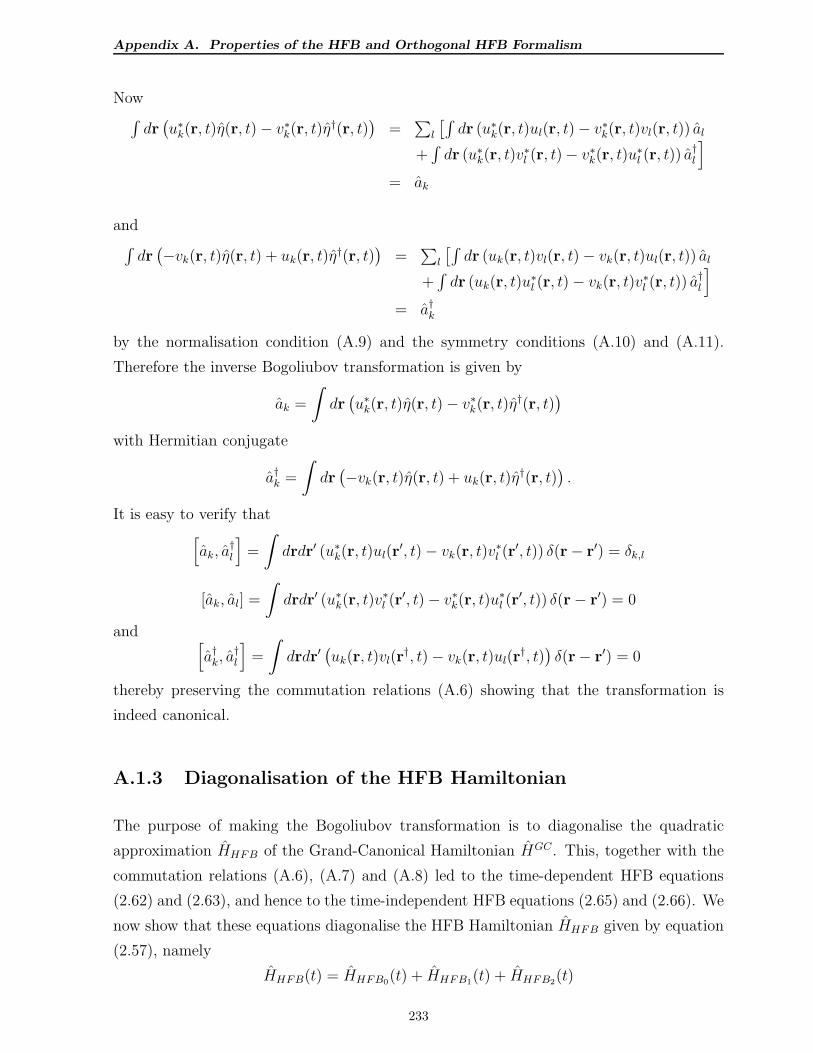
Appendix A. Properties of the HFB and Orthogonal HFB Formalism
Now∫
dr(
u∗k(r, t)η(r, t)− v∗k(r, t)η†(r, t))
=∑
l
[∫
dr (u∗k(r, t)ul(r, t)− v∗k(r, t)vl(r, t)) al
+∫
dr (u∗k(r, t)v∗l (r, t)− v∗k(r, t)u∗l (r, t)) a†l
]
= ak
and∫
dr(
−vk(r, t)η(r, t) + uk(r, t)η†(r, t)
)
=∑
l
[∫
dr (uk(r, t)vl(r, t)− vk(r, t)ul(r, t)) al
+∫
dr (uk(r, t)u∗l (r, t)− vk(r, t)v
∗l (r, t)) a
†l
]
= a†k
by the normalisation condition (A.9) and the symmetry conditions (A.10) and (A.11).
Therefore the inverse Bogoliubov transformation is given by
ak =
∫
dr(
u∗k(r, t)η(r, t)− v∗k(r, t)η†(r, t))
with Hermitian conjugate
a†k =
∫
dr(
−vk(r, t)η(r, t) + uk(r, t)η†(r, t)
)
.
It is easy to verify that[
ak, a†l
]
=
∫
drdr′ (u∗k(r, t)ul(r′, t)− vk(r, t)v
∗l (r
′, t)) δ(r− r′) = δk,l
[ak, al] =
∫
drdr′ (u∗k(r, t)v∗l (r
′, t)− v∗k(r, t)u∗l (r′, t)) δ(r− r′) = 0
and[
a†k, a†l
]
=
∫
drdr′(
uk(r, t)vl(r†, t)− vk(r, t)ul(r
†, t))
δ(r− r′) = 0
thereby preserving the commutation relations (A.6) showing that the transformation is
indeed canonical.
A.1.3 Diagonalisation of the HFB Hamiltonian
The purpose of making the Bogoliubov transformation is to diagonalise the quadratic
approximation HHFB of the Grand-Canonical Hamiltonian HGC. This, together with the
commutation relations (A.6), (A.7) and (A.8) led to the time-dependent HFB equations
(2.62) and (2.63), and hence to the time-independent HFB equations (2.65) and (2.66). We
now show that these equations diagonalise the HFB Hamiltonian HHFB given by equation
(2.57), namely
HHFB(t) = HHFB0(t) + HHFB1(t) + HHFB2(t)
233
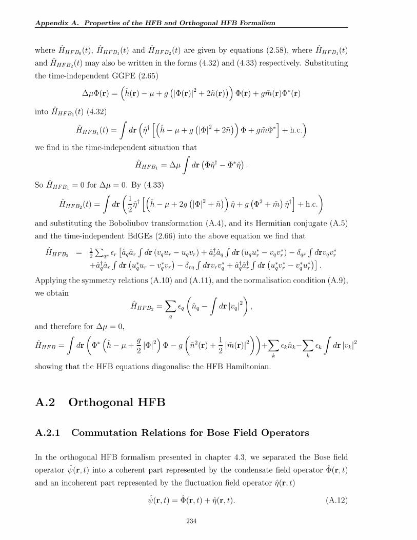
Appendix A. Properties of the HFB and Orthogonal HFB Formalism
where HHFB0(t), HHFB1(t) and HHFB2(t) are given by equations (2.58), where HHFB1(t)
and HHFB2(t) may also be written in the forms (4.32) and (4.33) respectively. Substituting
the time-independent GGPE (2.65)
∆µΦ(r) =(
h(r)− µ+ g(
|Φ(r)|2 + 2n(r))
)
Φ(r) + gm(r)Φ∗(r)
into HHFB1(t) (4.32)
HHFB1(t) =
∫
dr(
η†[(
h− µ+ g(
|Φ|2 + 2n)
)
Φ + gmΦ∗]
+ h.c.)
we find in the time-independent situation that
HHFB1 = ∆µ
∫
dr(
Φη† − Φ∗η)
.
So HHFB1 = 0 for ∆µ = 0. By (4.33)
HHFB2(t) =
∫
dr
(
1
2η†[(
h− µ+ 2g(
|Φ|2 + n)
)
η + g(
Φ2 + m)
η†]
+ h.c.
)
and substituting the Boboliubov transformation (A.4), and its Hermitian conjugate (A.5)
and the time-independent BdGEs (2.66) into the above equation we find that
HHFB2 = 12
∑
qr ǫr[
aqar
∫
dr (vqur − uqvr) + a†raq
∫
dr (uqu∗r − vqv
∗r )− δqr
∫
drvqv∗r
+a†qar
∫
dr(
u∗qur − v∗qvr
)
− δrq
∫
drvrv∗q + a†qa
†r
∫
dr(
u∗qv∗r − v∗qu∗r
)]
.
Applying the symmetry relations (A.10) and (A.11), and the normalisation condition (A.9),
we obtain
HHFB2 =∑
q
ǫq
(
nq −∫
dr |vq|2)
,
and therefore for ∆µ = 0,
HHFB =
∫
dr
(
Φ∗(
h− µ+g
2|Φ|2
)
Φ− g(
n2(r) +1
2|m(r)|2
))
+∑
k
ǫknk−∑
k
ǫk
∫
dr |vk|2
showing that the HFB equations diagonalise the HFB Hamiltonian.
A.2 Orthogonal HFB
A.2.1 Commutation Relations for Bose Field Operators
In the orthogonal HFB formalism presented in chapter 4.3, we separated the Bose field
operator ψ(r, t) into a coherent part represented by the condensate field operator Φ(r, t)
and an incoherent part represented by the fluctuation field operator η(r, t)
ψ(r, t) = Φ(r, t) + η(r, t). (A.12)
234
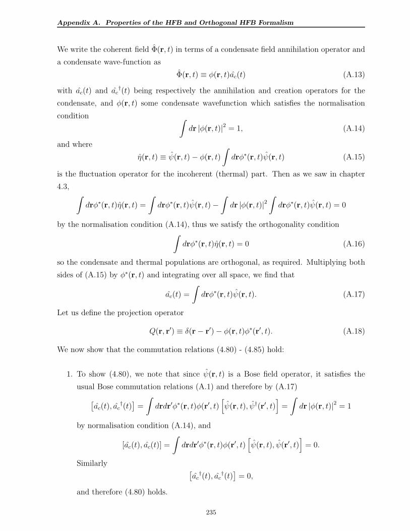
Appendix A. Properties of the HFB and Orthogonal HFB Formalism
We write the coherent field Φ(r, t) in terms of a condensate field annihilation operator and
a condensate wave-function as
Φ(r, t) ≡ φ(r, t)ac(t) (A.13)
with ac(t) and ac†(t) being respectively the annihilation and creation operators for the
condensate, and φ(r, t) some condensate wavefunction which satisfies the normalisation
condition∫
dr |φ(r, t)|2 = 1, (A.14)
and where
η(r, t) ≡ ψ(r, t)− φ(r, t)
∫
drφ∗(r, t)ψ(r, t) (A.15)
is the fluctuation operator for the incoherent (thermal) part. Then as we saw in chapter
4.3,∫
drφ∗(r, t)η(r, t) =
∫
drφ∗(r, t)ψ(r, t)−∫
dr |φ(r, t)|2∫
drφ∗(r, t)ψ(r, t) = 0
by the normalisation condition (A.14), thus we satisfy the orthogonality condition∫
drφ∗(r, t)η(r, t) = 0 (A.16)
so the condensate and thermal populations are orthogonal, as required. Multiplying both
sides of (A.15) by φ∗(r, t) and integrating over all space, we find that
ac(t) =
∫
drφ∗(r, t)ψ(r, t). (A.17)
Let us define the projection operator
Q(r, r′) ≡ δ(r− r′)− φ(r, t)φ∗(r′, t). (A.18)
We now show that the commutation relations (4.80) - (4.85) hold:
1. To show (4.80), we note that since ψ(r, t) is a Bose field operator, it satisfies the
usual Bose commutation relations (A.1) and therefore by (A.17)
[
ac(t), ac†(t)]
=
∫
drdr′φ∗(r, t)φ(r′, t)[
ψ(r, t), ψ†(r′, t)]
=
∫
dr |φ(r, t)|2 = 1
by normalisation condition (A.14), and
[ac(t), ac(t)] =
∫
drdr′φ∗(r, t)φ(r′, t)[
ψ(r, t), ψ(r′, t)]
= 0.
Similarly[
ac†(t), ac
†(t)]
= 0,
and therefore (4.80) holds.
235
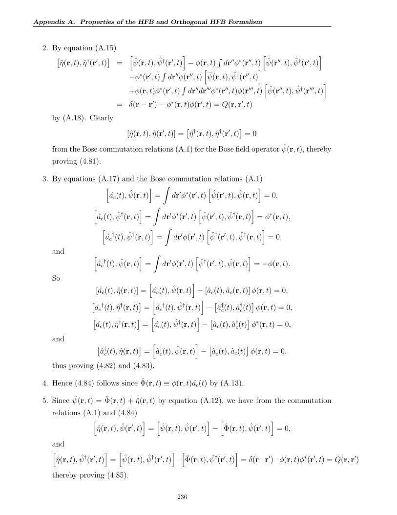
Appendix A. Properties of the HFB and Orthogonal HFB Formalism
2. By equation (A.15)[
η(r, t), η†(r′, t)]
=[
ψ(r, t), ψ†(r′, t)]
− φ(r, t)∫
dr′′φ∗(r′′, t)[
ψ(r′′, t), ψ†(r′, t)]
−φ∗(r′, t)∫
dr′′φ(r′′, t)[
ψ(r, t), ψ†(r′′, t)]
+φ(r, t)φ∗(r′, t)∫
dr′′dr′′′φ∗(r′′, t)φ(r′′′, t)[
ψ(r′′, t), ψ†(r′′′, t)]
= δ(r− r′)− φ∗(r, t)φ(r′, t) = Q(r, r′, t)
by (A.18). Clearly
[η(r, t), η(r′, t)] =[
η†(r, t), η†(r′, t)]
= 0
from the Bose commutation relations (A.1) for the Bose field operator ψ(r, t), thereby
proving (4.81).
3. By equations (A.17) and the Bose commutation relations (A.1)[
ac(t), ψ(r, t)]
=
∫
dr′φ∗(r′, t)[
ψ(r′, t), ψ(r, t)]
= 0,
[
ac(t), ψ†(r, t)
]
=
∫
dr′φ∗(r′, t)[
ψ(r′, t), ψ†(r, t)]
= φ∗(r, t),
[
ac†(t), ψ†(r, t)
]
=
∫
dr′φ(r′, t)[
ψ†(r′, t), ψ†(r, t)]
= 0,
and[
ac†(t), ψ(r, t)
]
=
∫
dr′φ(r′, t)[
ψ†(r′, t), ψ(r, t)]
= −φ(r, t).
So
[ac(t), η(r, t)] =[
ac(t), ψ(r, t)]
− [ac(t), ac(r, t)]φ(r, t) = 0,
[
ac†(t), η†(r, t)
]
=[
ac†(t), ψ†(r, t)
]
−[
a†c(t), a†c(t)]
φ(r, t) = 0,
[
ac(t), η†(r, t)
]
=[
ac(t), ψ†(r, t)
]
−[
ac(t), a†c(t)]
φ∗(r, t) = 0,
and[
a†c(t), η(r, t)]
=[
a†c(t), ψ(r, t)]
−[
a†c(t), ac(t)]
φ(r, t) = 0.
thus proving (4.82) and (4.83).
4. Hence (4.84) follows since Φ(r, t) ≡ φ(r, t)ac(t) by (A.13).
5. Since ψ(r, t) = Φ(r, t) + η(r, t) by equation (A.12), we have from the commutation
relations (A.1) and (4.84)[
η(r, t), ψ(r′, t)]
=[
ψ(r, t), ψ(r′, t)]
−[
Φ(r, t), ψ(r′, t)]
= 0,
and[
η(r, t), ψ†(r′, t)]
=[
ψ(r, t), ψ†(r′, t)]
−[
Φ(r, t), ψ†(r′, t)]
= δ(r−r′)−φ(r, t)φ∗(r′, t) = Q(r, r′)
thereby proving (4.85).
236
Appendix A. Properties of the HFB and Orthogonal HFB Formalism
A.2.2 Symmetry and Orthogonality Properties of the Bogoli-
ubov Transformation
We assume that the same symmetry and orthogonality properties of the Bogoliubov trans-
formation (A.4) and (A.5), given by equations (A.10), (A.11) and (A.9) respectively, hold
as for standard HFB.
A.2.3 Diagonalisation of the HFB Hamiltonian
Substituting the time-independent GGPE (4.106)
∆µΦ(r) =(
h(r)− µ+ g(
|Φ(r)|2 + 2n(r))
)
Φ(r) + gm(r)Φ∗(r)−∫
dr′P (r, r′)φ(r′)
(A.19)
into HHFB1(t) as given by equation (4.32) we find in the time-independent situation that
HHFB1 = ∆µ
∫
dr(
η†Φ + Φ∗η)
+
∫
dr
(
η†∫
dr′P (r, r′)φ(r′) + h.c.
)
≈ ∆µ
∫
dr(
η†Φ + Φ∗η)
to quadratic order in the fluctuation operator η, and therefore HHFB1 = 0 for ∆µ = 0. In
view of the orthogonality condition (4.77), we can write
HHFB2(t) =∫
dr
12η†(r)
∫
dr′Q(r, r′)[(
h(r′)− µ+ g(
|Φ(r′)|2 + 2n(r′))
)
η(r′)
+g (Φ2(r′) + m(r′)) η†(r′)]
+12
∫
dr′Q(r, r′)[(
h∗(r′)− µ+ g(
|Φ(r′)|2 + 2n(r′))
)
η†(r′)
+g(
Φ∗2(r′) + m∗(r′)
)
η(r′)]
η(r)
and substituting the Boboliubov transformation (A.4), and its Hermitian conjugate (A.5)
and the time-independent BdGEs (4.107) into the above equation we find that
HHFB2 = 12
∑
qr ǫr[
aqar
∫
dr (vqur − uqvr) + a†raq
∫
dr (uqu∗r − vqv
∗r)− δqr
∫
drvqv∗r
+a†qar
∫
dr(
u∗qur − v∗qvr
)
− δrq
∫
drvrv∗q + a†qa
†r
∫
dr(
u∗qv∗r − v∗qu∗r
)]
as before. Applying the symmetry relations (A.10) and (A.11), and the orthogonality
relation (A.9), we obtain
HHFB2 =∑
q
ǫq
(
nq −∫
dr |vq|2)
and therefore for ∆µ = 0,
HHFB =
∫
dr
(
Φ∗(
h− µ+g
2|Φ|2
)
Φ− g(
n(r) +1
2|m(r)|2
))
+∑
k
ǫknk−∑
k
ǫk
∫
dr |vk|2
237
Appendix A. Properties of the HFB and Orthogonal HFB Formalism
showing that the orthogonal HFB equations diagonalise the HFB Hamiltonian. Substitut-
ing the time-independent generalised GGPEs (A.19) into this equation gives us
HHFB =∫
drΦ∗ (−g(
12|Φ|2 + 2n
)
Φ− gmΦ∗
−g(
n(r) + 12|m(r)|2
))
+∑
k ǫknk −∑
k ǫk∫
dr |vk|2 ,
since∫
drΦ∗(r)∫
dr′Pk(r, r′)φk(r
′) = 0 , and hence we obtain (for ∆µ = 0)
HHFB =∑
k ǫknk − g∫
dr
Φ∗ [(12|Φ|2 + 2n
)
Φ]
+ 12
(
mΦ∗2+ m∗Φ2
)
+n+ 12|m|2
−∑k ǫk∫
dr |vk|2 .(A.20)
Let us define
IHFB = −g∫
dr
Φ∗ [(12|Φ|2 + 2n
)
Φ]
+ 12
(
mΦ∗2+ m∗Φ2
)
+n+ 12|m|2
−∑
k ǫk∫
dr |vk|2 .(A.21)
Then this simplifies to
HHFB = IHFB +∑
k
ǫknk. (A.22)
For ∆µ 6= 0 we find that
HHFB = IHFB + ∆µ
∫
dr(
η†Φ + Φ∗η)
+Nc∆µ+∑
k
ǫknk. (A.23)
A.3 Condensate and Quasi-particle Occupation Num-
bers
We first note that given the Grand Canonical Hamiltonian H(GC), the thermal average for
any operator O is given by [169]
⟨
O⟩
=Tr
O exp(
βH(GC))
Z (β)(A.24)
where Z (β) is the partition function for the Grand Canonical Hamiltonian H(GC) given by
Z (β) ≡ Tr
exp(
βH(GC))
. (A.25)
In what follows we make use of the following two results for any real number x such that
|x| < 1:
1.∑∞
n=1 xn = 1
1−x, and
238
Appendix A. Properties of the HFB and Orthogonal HFB Formalism
2. (1− x)∑∞
n=1 nxn = x
1−x.
Here H(GC) ≈ HHFB = IHFB +∆µ∫
dr(
η†Φ + Φ∗η)
+Nc∆µ+∑
q ǫqnq by equation (A.23),
where the integral IHFB is given by equation (A.21) above, and therefore1
Z (β) ≡ Tr
exp (−βIHFB) [exp (−βNc∆µ)]
[
∏
k
exp (−βnkǫk)
]
(A.26)
which we assume can be re-written as
Z (β) ≈ exp (−βIHFB)
[ ∞∑
Nc=0
exp (−βNc∆µ)
][
∏
k
∞∑
nk=1
exp (−βnkǫk)
]
(A.27)
where Nc is the condensate occupation number, and nk is the occupation number for the
kth quasi-particle excitation. We apply the definition (A.24) for the thermal average⟨
O⟩
of an operator O, and defining the thermal averages Nc ≡ 〈Nc〉 and nq ≡ 〈nq〉 for the
condensate and quasi-particle number operators Nc ≡ a†cac and nq ≡ a†qaq respectively, we
find (assuming that the integral IHFB contains purely thermally-averaged quantities, and
can therefore be factored out when tracing over Fock space) that
Nc ≈e−βIHF B
Z (β)
[ ∞∑
Nc=0
Nce−βNc∆µ
][
∏
k
∞∑
nk=1
e−βnkǫk
]
(A.28)
and
nq ≈e−βIHF B
Z (β)
[ ∞∑
Nc=0
e−βNc∆µ
][
∏
k 6=q
∞∑
nk=1
e−βnkǫk
]
∞∑
nq=0
nqe−βnkǫk
. (A.29)
Therefore by the results 1 and 2 above, we find that the thermal averages Nc and nq for
the condensate and quasiparticle occupation numbers obey the Bose distribution, i.e
Nc =1
exp (β∆µ)− 1
and
nq =1
exp (βǫq)− 1.
Here we drop the bars, and regard Nc as the thermal average for the occupation number
for the condensate, and nq as the thermal average for the quasi-particle number operator
1In what follows we assume that we can regard the quantities in IHFB as thermal averages which are
therefore unaffected when tracing over Fock space in evaluating the partition function Z (β) in equation
(A.26) and the quantities Nc and nq, and hence we can factor out the term exp (−βIHFB) as we have done
in equations (A.27), (A.28) and (A.29). We also note that the integral ∆µ∫
dr(
η†Φ + Φ∗η)
is traceless
since 〈n1 . . . nq . . .| aq |n1 . . . nq . . .〉 = 〈n1 . . . nq . . .| a†p |n1 . . . nq . . .〉 = 0 and therefore does not affect the
calculations for ensemble averages.
239
Appendix A. Properties of the HFB and Orthogonal HFB Formalism
〈nq〉 ≡⟨
a†qaq
⟩
. Thus we can write the occupation number Nc for the condensate in the
time-independent case as
Nc =1
exp (β∆µ)− 1(A.30)
and the occupation number Nq for thermal mode q as
Nq =
∫
dr(
nq |uq(r)|2 + (nq + 1) |vq(r)|2)
(A.31)
by equation (2.52), where we have shown that2
nq =1
exp (βǫq)− 1(A.32)
are the occupation numbers for quasiparticle q. Since by equation (A.30) the true value
for the chemical potential differs from the eigenvalue for the GGPE ground state by ∆µ,
we need to consider the fugacity term z = exp(
∆µkT
)
in the calculation of the quasi-particle
occupation numbers given by nq = NBE(ǫq) = 1z−1 exp(βǫq)−1
in chapter 4, section 4.2.3,
where the energies are with respect to the eigenvalue of the condensate ground state µ+∆µ,
and not the true chemical potential µ. Here ∆µ is the difference between the eigenvalue and
the true chemical potential. In cases where the quasi-particle energies are given with respect
to the true chemical potential, we use the expression (A.32) for the occupation numbers,
i.e. nq = 1exp(βǫq)−1
. As pointed out in chapter 4, ∆µ is negligible at low temperature, for
large Natoms, hence the fugacity term z = exp(
∆µkT
)
is very close to unity, and can therefore
be ignored.
2Note that for p 6= q, 〈n1 . . . np . . . nq . . .| a†paq |n1 . . . np . . . nq . . .〉 = 0, so⟨
a†paq
⟩
= nqδpq with nq given
by (A.32).
240
Appendix B. Conservation Laws for HFB and Orthogonal HFB
Appendix B
Conservation Laws for HFB and
Orthogonal HFB
B.1 Vector Calculus Results applied to Bose Field
Operators
B.1.1 Standard Results from Vector Calculus
Consider any volume V bounded by a surface S, and let φ(r) and ψ(r) be smooth scalar
fields and χ(r) a smooth vector field such that φ(r), ψ(r), and χ(r) and all their derivatives
vanish as r →∞. Then the following results hold:
1. By Green’s second identity, we have∫
V
dr(
φ(r)∇2ψ(r)− ψ(r)∇2φ(r))
=
∮
S
dS · (φ(r)∇ψ(r)− ψ(r)∇φ(r))
and since both φ(r) and ψ(r) and all their derivatives vanish as r →∞, integrating
over all space implies∮
SdS · (φ(r)∇ψ(r)− ψ(r)∇φ(r)) = 0, thus we obtain the result∫
drφ(r)∇2ψ(r) =
∫
drψ(r)∇2φ(r) (B.1)
where integration over all space is implied.
2. By the divergence theorem∫
V
dr∇ · χ(r) =
∮
S
dS · χ(r). (B.2)
241
Appendix B. Conservation Laws for HFB and Orthogonal HFB
3. It can be shown that the following standard identity∫
V
dr∇× χ(r) =
∮
S
dS× χ(r) (B.3)
holds.
4. Since χ(r) and all its derivatives vanish as r →∞, integrating over all space implies∮
SdS · χ(r) = 0 and therefore by (B.2)
∫
dr∇ · χ(r) = 0. (B.4)
Then for smooth scalar functions φ(r) and ψ(r) and any vector v,
v ·∫
dr (φ(r)∇ψ(r) + ψ(r)∇ψ(r)) =
∫
dr∇ · (vφ(r)ψ(r)) = 0
by (B.4) above, and therefore
v ·∫
drφ(r)∇ψ(r) = −v ·∫
drψ(r)∇ψ(r). (B.5)
5. We have
∇× (rφ(r)) = φ(r) (∇× r) = ∇φ(r)× r = −r× (∇φ(r))
since ∇× r = 0. Then by equation (B.3), it follows that
∫
V
dr (r×∇) (φ(r)ψ(r)) = −∮
S
dS× (rφ(r)ψ(r))
Since both φ(r) and ψ(r) and all their derivatives vanish as r →∞, integrating over
all space implies∮
SdS× (rφ(r)ψ(r)) = 0, and therefore for integration over all space
∫
dr (r×∇) (φ(r)ψ(r)) = 0
and therefore∫
drφ(r) (r×∇)ψ(r) = −∫
drψ(r) (r×∇)φ(r). (B.6)
B.1.2 Vector Calculus Results for Bose Field Operators
Let ψ(r, t) be a Bose field operator written as the sum of a condensate operator Φ(r, t)
corresponding to the coherent part, and a fluctuation operator part corresponding to the
thermal cloud (incoherent part), i.e. as ψ(r, t) = Φ(r, t)+η(r, t). We consider here standard
and orthogonal HFB where we assume a macroscopic occupation of the condensate, thus
242
Appendix B. Conservation Laws for HFB and Orthogonal HFB
Φ(r, t) =⟨
Φ(r, t)⟩
is the condensate wave-function. The fluctuation operator η(r, t) can
be written in the quasi-particle basis using the Bogoliubov transformation (2.43)
η(r, t) =∑
k
(
uk(r, t)ak + v∗k(r, t)a†k
)
(B.7)
where the a†k and the ak are respectively the quasi-particle creation and annihilation oper-
ators with the corresponding quasi-particle amplitude wave-functions uk(r, t) and v∗k(r, t).
Let hΩ(r) be the single-particle Hamiltonian in the rotating frame, and hv(r) be the single-
particle Hamiltonian in the rotating frame as defined in chapters 2 and 4. Then the fol-
lowing results hold:
1. For the Bose field operator ψ(r, t)
⟨∫
dr(
ψ†(r, t)hΩ(r)ψ(r, t)−(
h∗Ω(r)ψ†(r, t))
ψ(r, t))
⟩
= 0 (B.8)
2. For any linear differential operator D(r)
⟨∫
dr(
ψ†D(
hΩψ)
−(
h∗Ωψ†)
Dψ)
⟩
=
∫
dr(
|Φ|2 + n)
DVT (B.9)
where VT (r) is the trapping potential of the BEC.
3. For the Bose field operator ψ(r, t)
⟨∫
dr(
ψ†(r, t)hv(r)ψ(r, t)−(
h∗v(r)ψ†(r, t))
ψ(r, t))
⟩
= 0 (B.10)
4. For any linear differential operator D(r)
⟨∫
dr(
ψ†D(
hvψ)
−(
h∗vψ†)
Dψ)
⟩
=
∫
dr(
|Φ|2 + n)
DVT (B.11)
where VT (r) is the trapping potential of the BEC.
We now show that these results are true:
1. Proof of result 1:⟨
∫
dr(
ψ†hΩψ −(
h∗Ωψ†)
ψ)⟩
=∫
dr(
Φ∗hΩΦ− Φh∗ΩΦ∗)
+⟨
∫
dr(
η†hΩη −(
h∗Ωη†)
η)⟩
243
Appendix B. Conservation Laws for HFB and Orthogonal HFB
We first show that for any complex scalar fields φ(r, t) and ψ(r, t)∫
dr(
φ(r, t)hΩ(r)ψ(r, t)− ψ(r, t)h∗Ω(r)φ(r, t))
= 0 (B.12)
First note that the result∫
dr (φ∇2ψ − ψ∇2φ) = 0 follows by applying equation
(B.1) to the real and imaginary parts of φ(r, t) and ψ(r, t). We also note that∫
dr (φ (r×∇)ψ + ψ (r×∇)φ) =
∫
dr ((r×∇) (φψ)) = 0
follows by applying equation (B.6) to the real and imaginary parts of φ(r, t)ψ(r, t)
and clearly∫
dr (φVTψ − ψVTφ) = 0. Therefore the result∫
dr(
φhΩψ − ψh∗Ωφ)
= 0
holds for any complex scalar fields φ(r) and ψ(r) where the single-particle Hamilto-
nian in the rotating frame for trapping potential VT (r) is given by
hΩ(r) = − ~2
2m∇2
+ i~Ω · (r×∇) + VT (r). (B.13)
The result∫
dr(
Φ∗hΩΦ− Φh∗ΩΦ∗)
= 0 (B.14)
then follows. We now show that∫
dr(
η†hΩη −(
h∗Ωη†)
η)
= 0 (B.15)
thereby verifying equation (B.8). Using equation (B.7) and its Hermitian conjugate,
we see that
∫
dr(
η†hΩη −(
h∗Ωη†)
η)
=∑
kl
[
∫
dr(
vkhΩul − ulh∗Ωvk
)
akal
+∫
dr(
vkhΩv∗l − v∗l h∗Ωvk
)
aka†l
+∫
dr(
u∗khΩul − ulh∗Ωu
∗k
)
a†kal
+∫
dr(
u∗khΩv∗l − v∗l h∗Ωu∗k
)
a†ka†l
]
= 0
(B.16)
by equation (B.12), thus proving result 1 (equation (B.8)).
2. Proof of result 2:⟨
∫
dr(
ψ†D(
hΩψ)
−(
h∗Ωψ†)(
Dψ))⟩
=∫
dr(
Φ∗D(
hΩΦ)
−(
h∗ΩΦ∗)(
DΦ))
+⟨
∫
dr(
η†D(
hΩη)
−(
h∗Ωη†)(
Dη))⟩
(B.17)
We first show that for any complex scalar fields φ(r) and ψ(r)∫
dr(
φD(
hΩψ)
−(
h∗Ωφ)(
Dψ))
=
∫
drψφDVT . (B.18)
244
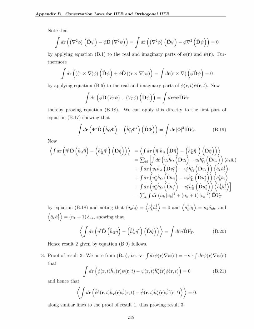
Appendix B. Conservation Laws for HFB and Orthogonal HFB
Note that∫
dr(
(
∇2φ)
(
Dψ)
− φD(
∇2ψ)
)
=
∫
dr(
(
∇2φ)
(
Dψ)
− φ∇2(
Dψ))
= 0
by applying equation (B.1) to the real and imaginary parts of φ(r) and ψ(r). Fur-
thermore∫
dr(
((r×∇)φ)(
Dψ)
+ φD ((r×∇)ψ))
=
∫
dr(r×∇)(
φDψ)
= 0
by applying equation (B.6) to the real and imaginary parts of φ(r, t)ψ(r, t). Now∫
dr(
φD (VTψ)− (VTφ)(
Dψ))
=
∫
drφψDVT
thereby proving equation (B.18). We can apply this directly to the first part of
equation (B.17) showing that∫
dr(
Φ∗D(
hΩΦ)
−(
h∗ΩΦ∗)(
DΦ))
=
∫
dr |Φ|2 DVT . (B.19)
Now⟨
∫
dr(
η†D(
hΩη)
−(
h∗Ωη†)(
Dη))⟩
=⟨
∫
dr(
η†hΩ
(
Dη)
−(
h∗Ωη†)(
Dη))⟩
=∑
kl
[
∫
dr(
vkhΩ
(
Dul
)
− ulh∗Ω
(
Dvk
))
〈akal〉+∫
dr(
vkhΩ
(
Dv∗l
)
− v∗l h∗Ω(
Dvk
))⟨
aka†l
⟩
+∫
dr(
u∗khΩ
(
Dul
)
− ulh∗Ω
(
Du∗k
))⟨
a†kal
⟩
+∫
dr(
u∗khΩ
(
Dv∗l
)
− v∗l h∗Ω(
Du∗k
))⟨
a†ka†l
⟩]
=∑
k
∫
dr(
nk |uk|2 + (nk + 1) |vk|2)
DVT
by equation (B.18) and noting that 〈akal〉 =⟨
a†ka†l
⟩
= 0 and⟨
a†kal
⟩
= nkδnk, and⟨
aka†l
⟩
= (nk + 1) δnk, showing that
⟨∫
dr(
η†D(
hΩη)
−(
h∗Ωη†)(
Dη))
⟩
=
∫
drnDVT . (B.20)
Hence result 2 given by equation (B.9) follows.
3. Proof of result 3: We note from (B.5), i.e. v ·∫
drφ(r)∇ψ(r) = −v ·∫
drψ(r)∇ψ(r)
that∫
dr(
φ(r, t)hv(r)ψ(r, t)− ψ(r, t)h∗v(r)φ(r, t))
= 0 (B.21)
and hence that⟨∫
dr(
ψ†(r, t)hv(r)ψ(r, t)− ψ(r, t)h∗v(r)ψ†(r, t))
⟩
= 0.
along similar lines to the proof of result 1, thus proving result 3.
245
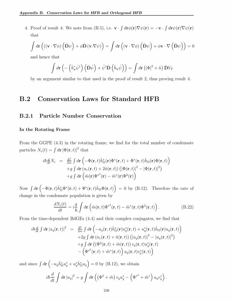
Appendix B. Conservation Laws for HFB and Orthogonal HFB
4. Proof of result 4: We note from (B.5), i.e. v ·∫
drφ(r)∇ψ(r) = −v ·∫
drψ(r)∇ψ(r)
that∫
dr(
((v · ∇φ)(
Dψ)
+ φD (v.∇ψ))
=
∫
dr(
(v · ∇φ)(
Dψ)
+ φv · ∇(
Dψ))
= 0
and hence that∫
dr(
−(
h∗vψ†)(
Dψ)
+ ψ†D(
hvψ))
=
∫
dr(
|Φ|2 + n)
DVT
by an argument similar to that used in the proof of result 2, thus proving result 4.
B.2 Conservation Laws for Standard HFB
B.2.1 Particle Number Conservation
In the Rotating Frame
From the GGPE (4.3) in the rotating frame, we find for the total number of condensate
particles Nc(t) =∫
dr |Φ(r, t)|2 that
i~ ddtNc = ~
2
2m
∫
dr(
−Φ(r, t)h∗Ω(r)Φ∗(r, t) + Φ∗(r, t)hΩ(r)Φ(r, t))
+g∫
dr (nc(r, t) + 2n(r, t))(
|Φ(r, t)|2 − |Φ(r, t)|2)
+g∫
dr(
m(r)Φ∗2(r)− m∗(r)Φ2(r)
)
Now∫
dr(
−Φ(r, t)h∗ΩΦ∗(r, t) + Φ∗(r, t)hΩΦ(r, t))
= 0 by (B.12). Therefore the rate of
change in the condensate population is given by
dNc(t)
dt= i
g
~
∫
dr(
m(r, t)Φ∗2
(r, t)− m∗(r, t)Φ2(r, t))
. (B.22)
From the time-dependent BdGEs (4.4) and their complex conjugates, we find that
i~ ddt
∫
dr |uq(r, t)|2 = ~2
2m
∫
dr(
−uq(r, t)h∗Ω(r)u∗q(r, t) + u∗q(r, t)hΩ(r)uq(r, t)
)
+2g∫
dr (nc(r, t) + n(r, t))(
|uq(r, t)|2 − |uq(r, t)|2)
+g∫
dr(
(Φ2(r, t) + m(r, t)) vq(r, t)u∗q(r, t)
−(
Φ∗2(r, t) + m∗(r, t)
)
uq(r, t)v∗q (r, t)
)
and since∫
dr(
−uqh∗Ωu
∗q + u∗qh
∗Ωuq
)
= 0 by (B.12), we obtain
i~d
dt
∫
dr |uq|2 = g
∫
dr(
(
Φ2 + m)
vqu∗q −
(
Φ∗2
+ m∗)
uqv∗q
)
.
246
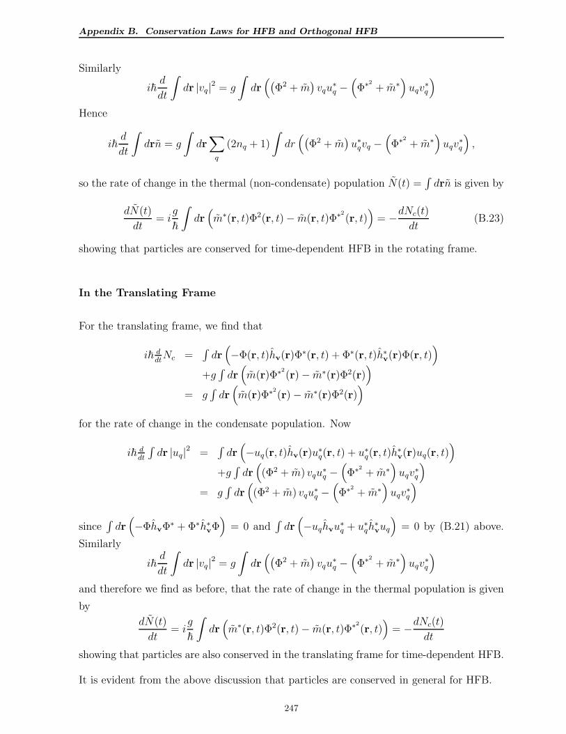
Appendix B. Conservation Laws for HFB and Orthogonal HFB
Similarly
i~d
dt
∫
dr |vq|2 = g
∫
dr(
(
Φ2 + m)
vqu∗q −
(
Φ∗2
+ m∗)
uqv∗q
)
Hence
i~d
dt
∫
drn = g
∫
dr∑
q
(2nq + 1)
∫
dr(
(
Φ2 + m)
u∗qvq −(
Φ∗2
+ m∗)
uqv∗q
)
,
so the rate of change in the thermal (non-condensate) population N(t) =∫
drn is given by
dN(t)
dt= i
g
~
∫
dr(
m∗(r, t)Φ2(r, t)− m(r, t)Φ∗2
(r, t))
= −dNc(t)
dt(B.23)
showing that particles are conserved for time-dependent HFB in the rotating frame.
In the Translating Frame
For the translating frame, we find that
i~ ddtNc =
∫
dr(
−Φ(r, t)hv(r)Φ∗(r, t) + Φ∗(r, t)h∗v(r)Φ(r, t))
+g∫
dr(
m(r)Φ∗2(r)− m∗(r)Φ2(r)
)
= g∫
dr(
m(r)Φ∗2(r)− m∗(r)Φ2(r)
)
for the rate of change in the condensate population. Now
i~ ddt
∫
dr |uq|2 =∫
dr(
−uq(r, t)hv(r)u∗q(r, t) + u∗q(r, t)h
∗v(r)uq(r, t)
)
+g∫
dr(
(Φ2 + m) vqu∗q −
(
Φ∗2+ m∗
)
uqv∗q
)
= g∫
dr(
(Φ2 + m) vqu∗q −
(
Φ∗2+ m∗
)
uqv∗q
)
since∫
dr(
−ΦhvΦ∗ + Φ∗h∗vΦ)
= 0 and∫
dr(
−uqhvu∗q + u∗qh
∗vuq
)
= 0 by (B.21) above.
Similarly
i~d
dt
∫
dr |vq|2 = g
∫
dr(
(
Φ2 + m)
vqu∗q −
(
Φ∗2
+ m∗)
uqv∗q
)
and therefore we find as before, that the rate of change in the thermal population is given
by
dN(t)
dt= i
g
~
∫
dr(
m∗(r, t)Φ2(r, t)− m(r, t)Φ∗2
(r, t))
= −dNc(t)
dt
showing that particles are also conserved in the translating frame for time-dependent HFB.
It is evident from the above discussion that particles are conserved in general for HFB.
247
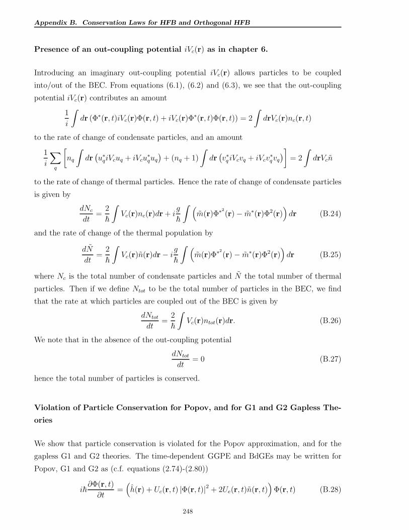
Appendix B. Conservation Laws for HFB and Orthogonal HFB
Presence of an out-coupling potential iVc(r) as in chapter 6.
Introducing an imaginary out-coupling potential iVc(r) allows particles to be coupled
into/out of the BEC. From equations (6.1), (6.2) and (6.3), we see that the out-coupling
potential iVc(r) contributes an amount
1
i
∫
dr (Φ∗(r, t)iVc(r)Φ(r, t) + iVc(r)Φ∗(r, t)Φ(r, t)) = 2
∫
drVc(r)nc(r, t)
to the rate of change of condensate particles, and an amount
1
i
∑
q
[
nq
∫
dr(
u∗qiVcuq + iVcu∗quq
)
+ (nq + 1)
∫
dr(
v∗q iVcvq + iVcv∗qvq
)
]
= 2
∫
drVcn
to the rate of change of thermal particles. Hence the rate of change of condensate particles
is given by
dNc
dt=
2
~
∫
Vc(r)nc(r)dr + ig
~
∫
(
m(r)Φ∗2
(r)− m∗(r)Φ2(r))
dr (B.24)
and the rate of change of the thermal population by
dN
dt=
2
~
∫
Vc(r)n(r)dr− ig~
∫
(
m(r)Φ∗2
(r)− m∗(r)Φ2(r))
dr (B.25)
where Nc is the total number of condensate particles and N the total number of thermal
particles. Then if we define Ntot to be the total number of particles in the BEC, we find
that the rate at which particles are coupled out of the BEC is given by
dNtot
dt=
2
~
∫
Vc(r)ntot(r)dr. (B.26)
We note that in the absence of the out-coupling potential
dNtot
dt= 0 (B.27)
hence the total number of particles is conserved.
Violation of Particle Conservation for Popov, and for G1 and G2 Gapless The-
ories
We show that particle conservation is violated for the Popov approximation, and for the
gapless G1 and G2 theories. The time-dependent GGPE and BdGEs may be written for
Popov, G1 and G2 as (c.f. equations (2.74)-(2.80))
i~∂Φ(r, t)
∂t=(
h(r) + Uc(r, t) |Φ(r, t)|2 + 2Ue(r, t)n(r, t))
Φ(r, t) (B.28)
248
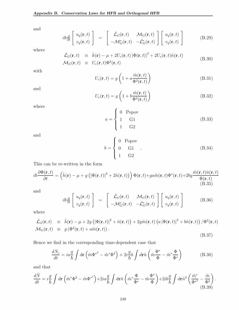
Appendix B. Conservation Laws for HFB and Orthogonal HFB
and
i~ ∂∂t
[
uq(r, t)
vq(r, t)
]
=
[
LG(r, t) MG(r, t)
−M∗G(r, t) −L∗
G(r, t)
][
uq(r, t)
vq(r, t)
]
(B.29)
whereLG(r, t) ≡ h(r)− µ+ 2Uc(r, t) |Φ(r, t)|2 + 2Ue(r, t)n(r, t)
MG(r, t) ≡ Uc(r, t)Φ2(r, t)
(B.30)
with
Uc(r, t) = g
(
1 + am(r, t)
Φ2(r, t)
)
(B.31)
and
Ue(r, t) = g
(
1 + bm(r, t)
Φ2(r, t)
)
(B.32)
where
a =
0 Popov
1 G1
1 G2
(B.33)
and
b =
0 Popov
0 G1
1 G2
. (B.34)
This can be re-written in the form
i~∂Φ(r, t)
∂t=(
h(r)− µ+ g(
|Φ(r, t)|2 + 2n(r, t))
)
Φ(r, t)+gam(r, t)Φ∗(r, t)+2bgm(r, t)n(r, t)
Φ(r, t)(B.35)
and
i~ ∂∂t
[
uq(r, t)
vq(r, t)
]
=
[
LG(r, t) MG(r, t)
−M∗G(r, t) −L∗
G(r, t)
][
uq(r, t)
vq(r, t)
]
(B.36)
where
LG(r, t) ≡ h(r)− µ+ 2g(
|Φ(r, t)|2 + n(r, t))
+ 2gm(r, t)(
a |Φ(r, t)|2 + bn(r, t))
/Φ2(r, t)
MG(r, t) ≡ g (Φ2(r, t) + am(r, t)) .
(B.37)
Hence we find in the corresponding time-dependent case that
dNc
dt= ia
g
~
∫
dr(
mΦ∗2 − m∗Φ2)
+ 2ig
~b
∫
drn
(
mΦ∗
Φ− m∗ Φ
Φ∗
)
(B.38)
and that
dN
dt= i
g
~
∫
dr(
m∗Φ2 − mΦ∗2)
+2iag
~
∫
drn
(
m∗ Φ
Φ∗ − mΦ∗
Φ
)
+2ibg
~
∫
drn2
(
m∗
Φ∗2 −m
Φ2
)
.
(B.39)
249
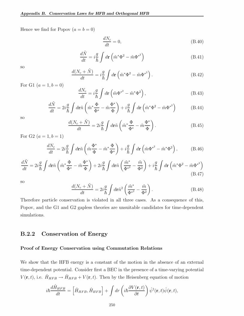
Appendix B. Conservation Laws for HFB and Orthogonal HFB
Hence we find for Popov (a = b = 0)
dNc
dt= 0, (B.40)
dN
dt= i
g
~
∫
dr(
m∗Φ2 − mΦ∗2)
(B.41)
sod(Nc + N)
dt= i
g
~
∫
dr(
m∗Φ2 − mΦ∗2)
. (B.42)
For G1 (a = 1, b = 0)dNc
dt= i
g
~
∫
dr(
mΦ∗2 − m∗Φ2)
, (B.43)
dN
dt= 2i
g
~
∫
drn
(
m∗ Φ
Φ∗ − mΦ∗
Φ
)
+ ig
~
∫
dr(
m∗Φ2 − mΦ∗2)
(B.44)
sod(Nc + N)
dt= 2i
g
~
∫
drn
(
m∗ Φ
Φ∗ − mΦ∗
Φ
)
. (B.45)
For G2 (a = 1, b = 1)
dNc
dt= 2i
g
~
∫
drn
(
mΦ∗
Φ− m∗ Φ
Φ∗
)
+ ig
~
∫
dr(
mΦ∗2 − m∗Φ2)
, (B.46)
dN
dt= 2i
g
~
∫
drn
(
m∗ Φ
Φ∗ − mΦ∗
Φ
)
+ 2ig
~
∫
drn
(
m∗
Φ∗2 −m
Φ2
)
+ ig
~
∫
dr(
m∗Φ2 − mΦ∗2)
(B.47)
sod(Nc + N)
dt= 2i
g
~
∫
drn2
(
m∗
Φ∗2 −m
Φ2
)
. (B.48)
Therefore particle conservation is violated in all three cases. As a consequence of this,
Popov, and the G1 and G2 gapless theories are unsuitable candidates for time-dependent
simulations.
B.2.2 Conservation of Energy
Proof of Energy Conservation using Commutation Relations
We show that the HFB energy is a constant of the motion in the absence of an external
time-dependent potential. Consider first a BEC in the presence of a time-varying potential
V (r, t), i.e. HHFB → HHFB + V (r, t). Then by the Heisenberg equation of motion
i~dHHFB
dt=[
HHFB, HHFB
]
+
∫
dr
(
i~∂V (r, t)
∂t
)
ψ†(r, t)ψ(r, t),
250
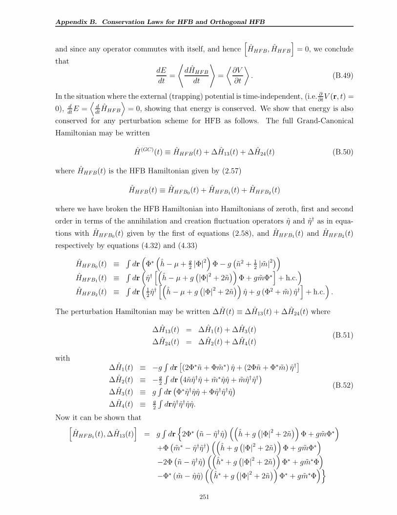
Appendix B. Conservation Laws for HFB and Orthogonal HFB
and since any operator commutes with itself, and hence[
HHFB, HHFB
]
= 0, we conclude
thatdE
dt=
⟨
dHHFB
dt
⟩
=
⟨
∂V
∂t
⟩
. (B.49)
In the situation where the external (trapping) potential is time-independent, (i.e. ∂∂tV (r, t) =
0), ddtE =
⟨
ddtHHFB
⟩
= 0, showing that energy is conserved. We show that energy is also
conserved for any perturbation scheme for HFB as follows. The full Grand-Canonical
Hamiltonian may be written
H(GC)(t) ≡ HHFB(t) + ∆H13(t) + ∆H24(t) (B.50)
where HHFB(t) is the HFB Hamiltonian given by (2.57)
HHFB(t) ≡ HHFB0(t) + HHFB1(t) + HHFB2(t)
where we have broken the HFB Hamiltonian into Hamiltonians of zeroth, first and second
order in terms of the annihilation and creation fluctuation operators η and η† as in equa-
tions with HHFB0(t) given by the first of equations (2.58), and HHFB1(t) and HHFB2(t)
respectively by equations (4.32) and (4.33)
HHFB0(t) ≡∫
dr(
Φ∗(
h− µ+ g2|Φ|2
)
Φ− g(
n2 + 12|m|2
)
)
HHFB1(t) ≡∫
dr(
η†[(
h− µ+ g(
|Φ|2 + 2n)
)
Φ + gmΦ∗]
+ h.c.)
HHFB2(t) ≡∫
dr(
12η†[(
h− µ+ g(
|Φ|2 + 2n)
)
η + g (Φ2 + m) η†]
+ h.c.)
.
The perturbation Hamiltonian may be written ∆H(t) ≡ ∆H13(t) + ∆H24(t) where
∆H13(t) = ∆H1(t) + ∆H3(t)
∆H24(t) = ∆H2(t) + ∆H4(t)(B.51)
with∆H1(t) ≡ −g
∫
dr[
(2Φ∗n + Φm∗) η + (2Φn + Φ∗m) η†]
∆H2(t) ≡ −g2
∫
dr(
4nη†η + m∗ηη + mη†η†)
∆H3(t) ≡ g∫
dr(
Φ∗η†ηη + Φη†η†η)
∆H4(t) ≡ g2
∫
drη†η†ηη.
(B.52)
Now it can be shown that[
HHFB1(t),∆H13(t)]
= g∫
dr
2Φ∗ (n− η†η)
((
h+ g(
|Φ|2 + 2n)
)
Φ + gmΦ∗)
+Φ(
m∗ − η†η†)
((
h+ g(
|Φ|2 + 2n)
)
Φ + gmΦ∗)
−2Φ(
n− η†η)
((
h∗ + g(
|Φ|2 + 2n)
)
Φ∗ + gm∗Φ)
−Φ∗ (m− ηη)((
h∗ + g(
|Φ|2 + 2n)
)
Φ∗ + gm∗Φ)
251
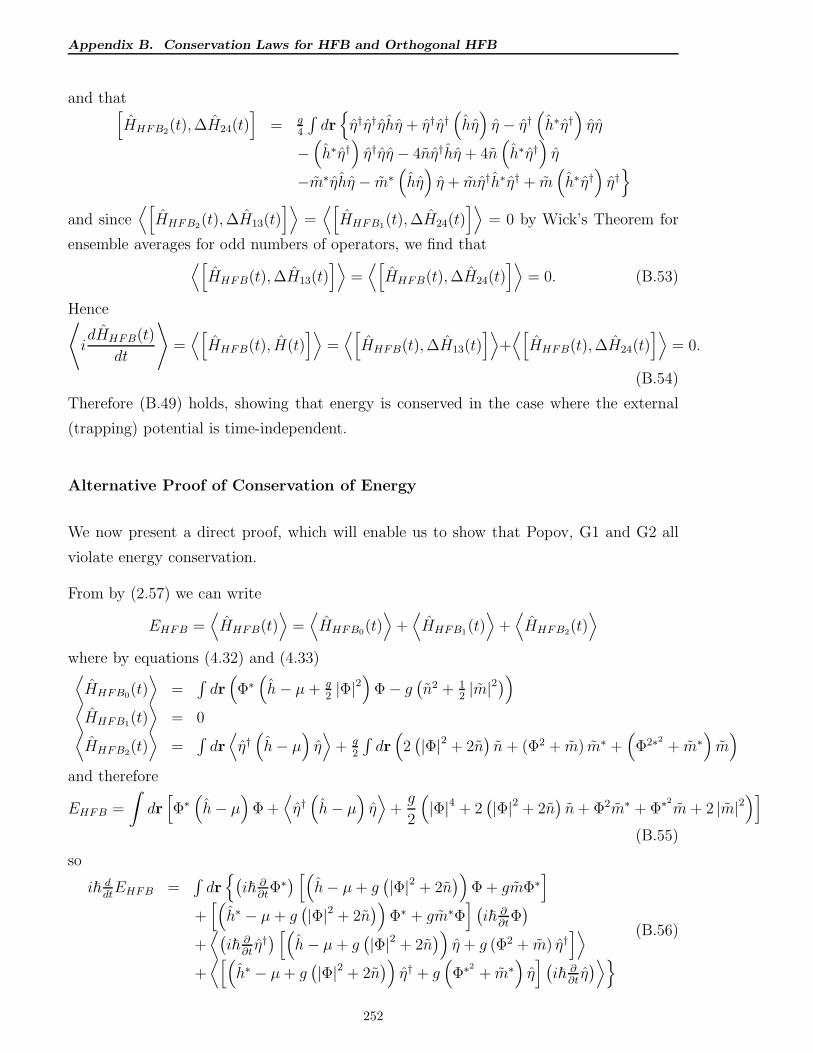
Appendix B. Conservation Laws for HFB and Orthogonal HFB
and that[
HHFB2(t),∆H24(t)]
= g4
∫
dr
η†η†ηhη + η†η†(
hη)
η − η†(
h∗η†)
ηη
−(
h∗η†)
η†ηη − 4nη†hη + 4n(
h∗η†)
η
−m∗ηhη − m∗(
hη)
η + mη†h∗η† + m(
h∗η†)
η†
and since⟨[
HHFB2(t),∆H13(t)]⟩
=⟨[
HHFB1(t),∆H24(t)]⟩
= 0 by Wick’s Theorem for
ensemble averages for odd numbers of operators, we find that⟨[
HHFB(t),∆H13(t)]⟩
=⟨[
HHFB(t),∆H24(t)]⟩
= 0. (B.53)
Hence⟨
idHHFB(t)
dt
⟩
=⟨[
HHFB(t), H(t)]⟩
=⟨[
HHFB(t),∆H13(t)]⟩
+⟨[
HHFB(t),∆H24(t)]⟩
= 0.
(B.54)
Therefore (B.49) holds, showing that energy is conserved in the case where the external
(trapping) potential is time-independent.
Alternative Proof of Conservation of Energy
We now present a direct proof, which will enable us to show that Popov, G1 and G2 all
violate energy conservation.
From by (2.57) we can write
EHFB =⟨
HHFB(t)⟩
=⟨
HHFB0(t)⟩
+⟨
HHFB1(t)⟩
+⟨
HHFB2(t)⟩
where by equations (4.32) and (4.33)⟨
HHFB0(t)⟩
=∫
dr(
Φ∗(
h− µ+ g2|Φ|2
)
Φ− g(
n2 + 12|m|2
)
)
⟨
HHFB1(t)⟩
= 0⟨
HHFB2(t)⟩
=∫
dr⟨
η†(
h− µ)
η⟩
+ g2
∫
dr(
2(
|Φ|2 + 2n)
n + (Φ2 + m) m∗ +(
Φ2∗2+ m∗
)
m)
and therefore
EHFB =
∫
dr[
Φ∗(
h− µ)
Φ +⟨
η†(
h− µ)
η⟩
+g
2
(
|Φ|4 + 2(
|Φ|2 + 2n)
n+ Φ2m∗ + Φ∗2
m+ 2 |m|2)]
(B.55)
so
i~ ddtEHFB =
∫
dr
(
i~ ∂∂t
Φ∗)[(
h− µ+ g(
|Φ|2 + 2n)
)
Φ + gmΦ∗]
+[(
h∗ − µ+ g(
|Φ|2 + 2n)
)
Φ∗ + gm∗Φ]
(
i~ ∂∂t
Φ)
+⟨
(
i~ ∂∂tη†)
[(
h− µ+ g(
|Φ|2 + 2n)
)
η + g (Φ2 + m) η†]⟩
+⟨[(
h∗ − µ+ g(
|Φ|2 + 2n)
)
η† + g(
Φ∗2+ m∗
)
η]
(
i~ ∂∂tη)
⟩
(B.56)
252
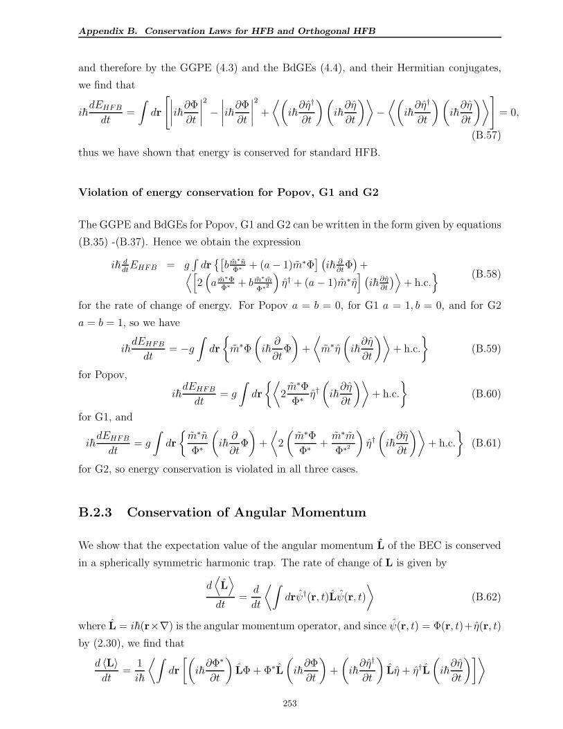
Appendix B. Conservation Laws for HFB and Orthogonal HFB
and therefore by the GGPE (4.3) and the BdGEs (4.4), and their Hermitian conjugates,
we find that
i~dEHFB
dt=
∫
dr
[
∣
∣
∣
∣
i~∂Φ
∂t
∣
∣
∣
∣
2
−∣
∣
∣
∣
i~∂Φ
∂t
∣
∣
∣
∣
2
+
⟨(
i~∂η†
∂t
)(
i~∂η
∂t
)⟩
−⟨(
i~∂η†
∂t
)(
i~∂η
∂t
)⟩
]
= 0,
(B.57)
thus we have shown that energy is conserved for standard HFB.
Violation of energy conservation for Popov, G1 and G2
The GGPE and BdGEs for Popov, G1 and G2 can be written in the form given by equations
(B.35) -(B.37). Hence we obtain the expression
i~ ddtEHFB = g
∫
dr[
b m∗nΦ∗ + (a− 1)m∗Φ
] (
i~ ∂∂t
Φ)
+⟨[
2(
a m∗ΦΦ∗ + b m∗m
Φ∗2
)
η† + (a− 1)m∗η]
(
i~∂η∂t
)
⟩
+ h.c. (B.58)
for the rate of change of energy. For Popov a = b = 0, for G1 a = 1, b = 0, and for G2
a = b = 1, so we have
i~dEHFB
dt= −g
∫
dr
m∗Φ
(
i~∂
∂tΦ
)
+
⟨
m∗η
(
i~∂η
∂t
)⟩
+ h.c.
(B.59)
for Popov,
i~dEHFB
dt= g
∫
dr
⟨
2m∗Φ
Φ∗ η†(
i~∂η
∂t
)⟩
+ h.c.
(B.60)
for G1, and
i~dEHFB
dt= g
∫
dr
m∗n
Φ∗
(
i~∂
∂tΦ
)
+
⟨
2
(
m∗Φ
Φ∗ +m∗m
Φ∗2
)
η†(
i~∂η
∂t
)⟩
+ h.c.
(B.61)
for G2, so energy conservation is violated in all three cases.
B.2.3 Conservation of Angular Momentum
We show that the expectation value of the angular momentum L of the BEC is conserved
in a spherically symmetric harmonic trap. The rate of change of L is given by
d⟨
L⟩
dt=
d
dt
⟨∫
drψ†(r, t)Lψ(r, t)
⟩
(B.62)
where L = i~(r×∇) is the angular momentum operator, and since ψ(r, t) = Φ(r, t)+ η(r, t)
by (2.30), we find that
d 〈L〉dt
=1
i~
⟨∫
dr
[(
i~∂Φ∗
∂t
)
LΦ + Φ∗L
(
i~∂Φ
∂t
)
+
(
i~∂η†
∂t
)
Lη + η†L
(
i~∂η
∂t
)]⟩
253
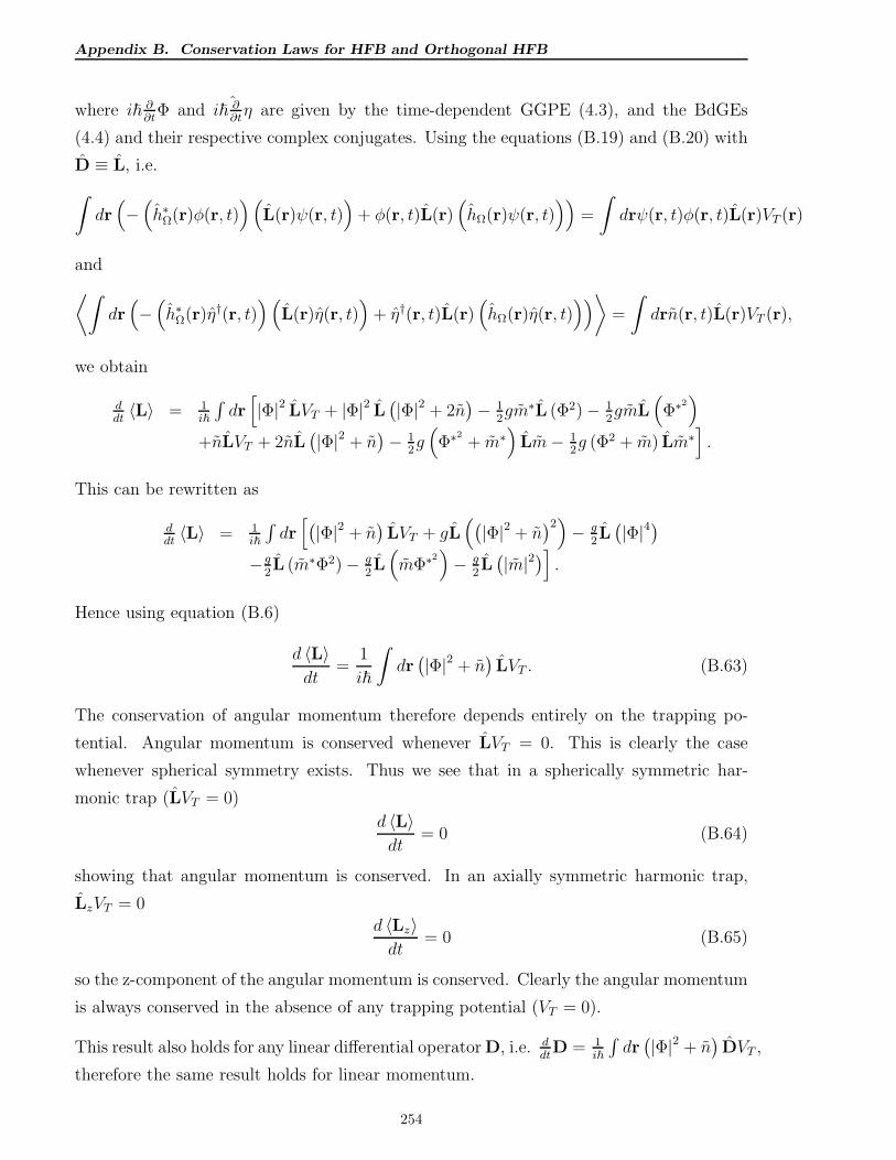
Appendix B. Conservation Laws for HFB and Orthogonal HFB
where i~ ∂∂t
Φ and ˆi~ ∂∂tη are given by the time-dependent GGPE (4.3), and the BdGEs
(4.4) and their respective complex conjugates. Using the equations (B.19) and (B.20) with
D ≡ L, i.e.
∫
dr(
−(
h∗Ω(r)φ(r, t))(
L(r)ψ(r, t))
+ φ(r, t)L(r)(
hΩ(r)ψ(r, t)))
=
∫
drψ(r, t)φ(r, t)L(r)VT (r)
and
⟨∫
dr(
−(
h∗Ω(r)η†(r, t))(
L(r)η(r, t))
+ η†(r, t)L(r)(
hΩ(r)η(r, t)))
⟩
=
∫
drn(r, t)L(r)VT (r),
we obtain
ddt〈L〉 = 1
i~
∫
dr[
|Φ|2 LVT + |Φ|2 L(
|Φ|2 + 2n)
− 12gm∗L (Φ2)− 1
2gmL
(
Φ∗2)
+nLVT + 2nL(
|Φ|2 + n)
− 12g(
Φ∗2+ m∗
)
Lm− 12g (Φ2 + m) Lm∗
]
.
This can be rewritten as
ddt〈L〉 = 1
i~
∫
dr[
(
|Φ|2 + n)
LVT + gL(
(
|Φ|2 + n)2)
− g2L(
|Φ|4)
−g2L (m∗Φ2)− g
2L(
mΦ∗2)
− g2L(
|m|2)
]
.
Hence using equation (B.6)
d 〈L〉dt
=1
i~
∫
dr(
|Φ|2 + n)
LVT . (B.63)
The conservation of angular momentum therefore depends entirely on the trapping po-
tential. Angular momentum is conserved whenever LVT = 0. This is clearly the case
whenever spherical symmetry exists. Thus we see that in a spherically symmetric har-
monic trap (LVT = 0)
d 〈L〉dt
= 0 (B.64)
showing that angular momentum is conserved. In an axially symmetric harmonic trap,
LzVT = 0
d 〈Lz〉dt
= 0 (B.65)
so the z-component of the angular momentum is conserved. Clearly the angular momentum
is always conserved in the absence of any trapping potential (VT = 0).
This result also holds for any linear differential operator D, i.e. ddtD = 1
i~
∫
dr(
|Φ|2 + n)
DVT ,
therefore the same result holds for linear momentum.
254
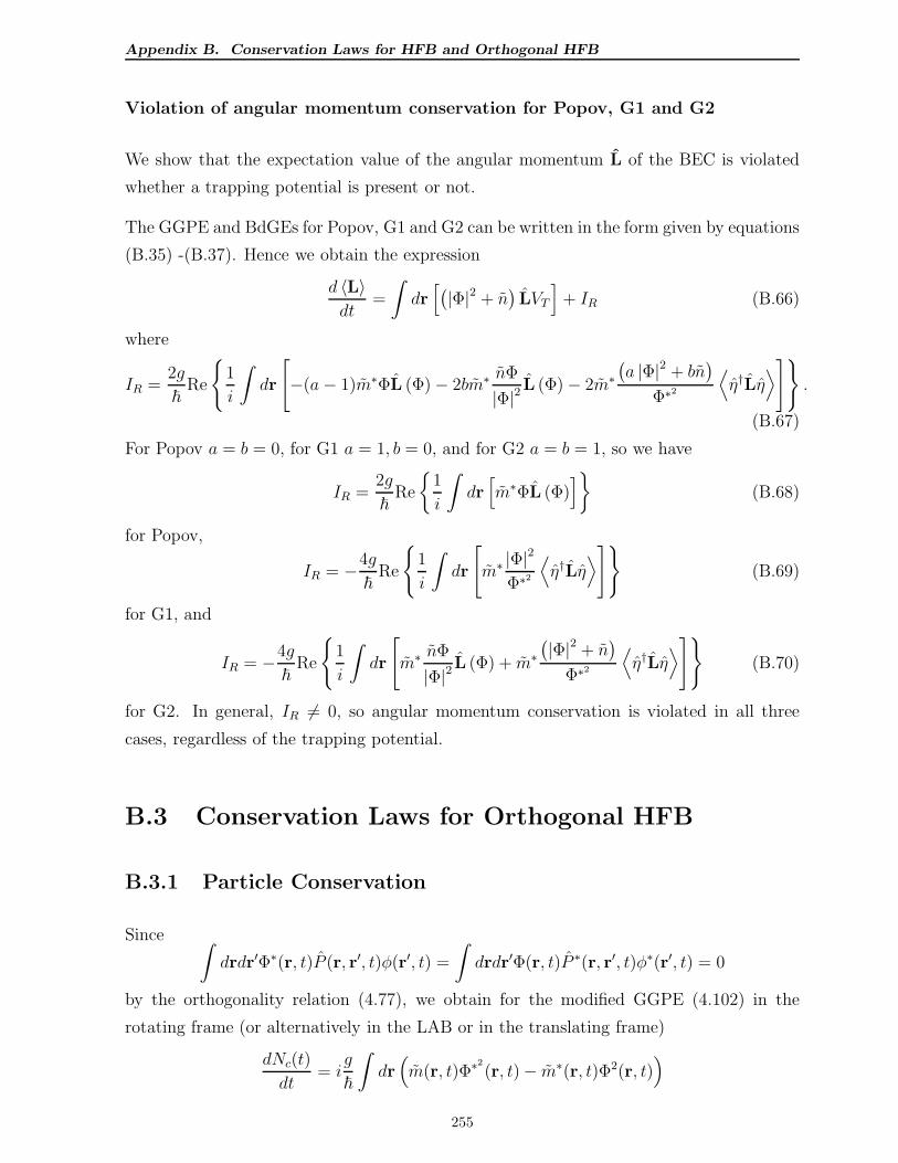
Appendix B. Conservation Laws for HFB and Orthogonal HFB
Violation of angular momentum conservation for Popov, G1 and G2
We show that the expectation value of the angular momentum L of the BEC is violated
whether a trapping potential is present or not.
The GGPE and BdGEs for Popov, G1 and G2 can be written in the form given by equations
(B.35) -(B.37). Hence we obtain the expression
d 〈L〉dt
=
∫
dr[
(
|Φ|2 + n)
LVT
]
+ IR (B.66)
where
IR =2g
~Re
1
i
∫
dr
[
−(a− 1)m∗ΦL (Φ)− 2bm∗ nΦ
|Φ|2L (Φ)− 2m∗
(
a |Φ|2 + bn)
Φ∗2
⟨
η†Lη⟩
]
.
(B.67)
For Popov a = b = 0, for G1 a = 1, b = 0, and for G2 a = b = 1, so we have
IR =2g
~Re
1
i
∫
dr[
m∗ΦL (Φ)]
(B.68)
for Popov,
IR = −4g
~Re
1
i
∫
dr
[
m∗ |Φ|2
Φ∗2
⟨
η†Lη⟩
]
(B.69)
for G1, and
IR = −4g
~Re
1
i
∫
dr
[
m∗ nΦ
|Φ|2L (Φ) + m∗
(
|Φ|2 + n)
Φ∗2
⟨
η†Lη⟩
]
(B.70)
for G2. In general, IR 6= 0, so angular momentum conservation is violated in all three
cases, regardless of the trapping potential.
B.3 Conservation Laws for Orthogonal HFB
B.3.1 Particle Conservation
Since∫
drdr′Φ∗(r, t)P (r, r′, t)φ(r′, t) =
∫
drdr′Φ(r, t)P ∗(r, r′, t)φ∗(r′, t) = 0
by the orthogonality relation (4.77), we obtain for the modified GGPE (4.102) in the
rotating frame (or alternatively in the LAB or in the translating frame)
dNc(t)
dt= i
g
~
∫
dr(
m(r, t)Φ∗2
(r, t)− m∗(r, t)Φ2(r, t))
255
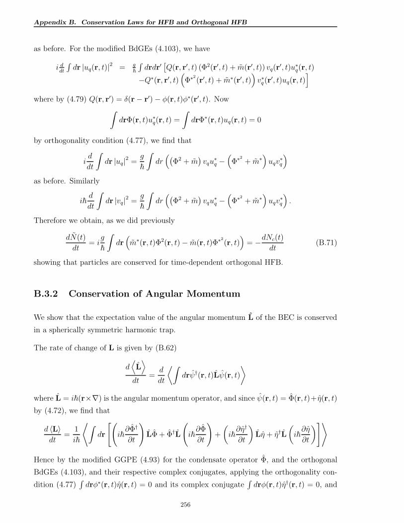
Appendix B. Conservation Laws for HFB and Orthogonal HFB
as before. For the modified BdGEs (4.103), we have
i ddt
∫
dr |uq(r, t)|2 = g~
∫
drdr′[
Q(r, r′, t) (Φ2(r′, t) + m(r′, t)) vq(r′, t)u∗q(r, t)
−Q∗(r, r′, t)(
Φ∗2(r′, t) + m∗(r′, t)
)
v∗q (r′, t)uq(r, t)
]
where by (4.79) Q(r, r′) = δ(r− r′)− φ(r, t)φ∗(r′, t). Now
∫
drΦ(r, t)u∗q(r, t) =
∫
drΦ∗(r, t)uq(r, t) = 0
by orthogonality condition (4.77), we find that
id
dt
∫
dr |uq|2 =g
~
∫
dr(
(
Φ2 + m)
vqu∗q −
(
Φ∗2
+ m∗)
uqv∗q
)
as before. Similarly
i~d
dt
∫
dr |vq|2 =g
~
∫
dr(
(
Φ2 + m)
vqu∗q −
(
Φ∗2
+ m∗)
uqv∗q
)
.
Therefore we obtain, as we did previously
dN(t)
dt= i
g
~
∫
dr(
m∗(r, t)Φ2(r, t)− m(r, t)Φ∗2
(r, t))
= −dNc(t)
dt(B.71)
showing that particles are conserved for time-dependent orthogonal HFB.
B.3.2 Conservation of Angular Momentum
We show that the expectation value of the angular momentum L of the BEC is conserved
in a spherically symmetric harmonic trap.
The rate of change of L is given by (B.62)
d⟨
L⟩
dt=
d
dt
⟨∫
drψ†(r, t)Lψ(r, t)
⟩
where L = i~(r×∇) is the angular momentum operator, and since ψ(r, t) = Φ(r, t)+ η(r, t)
by (4.72), we find that
d 〈L〉dt
=1
i~
⟨
∫
dr
[(
i~∂Φ†
∂t
)
LΦ + Φ†L
(
i~∂Φ
∂t
)
+
(
i~∂η†
∂t
)
Lη + η†L
(
i~∂η
∂t
)
]⟩
Hence by the modified GGPE (4.93) for the condensate operator Φ, and the orthogonal
BdGEs (4.103), and their respective complex conjugates, applying the orthogonality con-
dition (4.77)∫
drφ∗(r, t)η(r, t) = 0 and its complex conjugate∫
drφ(r, t)η†(r, t) = 0, and
256
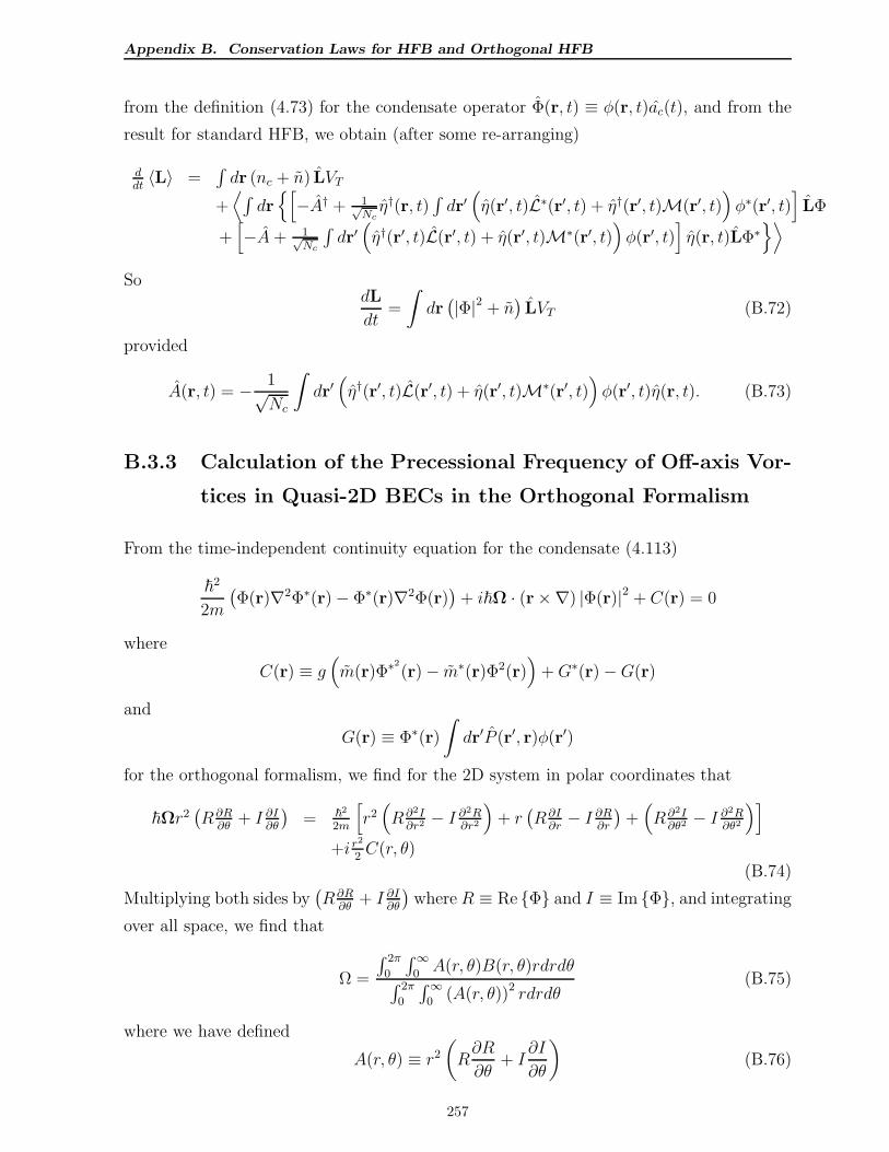
Appendix B. Conservation Laws for HFB and Orthogonal HFB
from the definition (4.73) for the condensate operator Φ(r, t) ≡ φ(r, t)ac(t), and from the
result for standard HFB, we obtain (after some re-arranging)
ddt〈L〉 =
∫
dr (nc + n) LVT
+⟨
∫
dr[
−A† + 1√Ncη†(r, t)
∫
dr′(
η(r′, t)L∗(r′, t) + η†(r′, t)M(r′, t))
φ∗(r′, t)]
LΦ
+[
−A+ 1√Nc
∫
dr′(
η†(r′, t)L(r′, t) + η(r′, t)M∗(r′, t))
φ(r′, t)]
η(r, t)LΦ∗⟩
SodL
dt=
∫
dr(
|Φ|2 + n)
LVT (B.72)
provided
A(r, t) = − 1√Nc
∫
dr′(
η†(r′, t)L(r′, t) + η(r′, t)M∗(r′, t))
φ(r′, t)η(r, t). (B.73)
B.3.3 Calculation of the Precessional Frequency of Off-axis Vor-
tices in Quasi-2D BECs in the Orthogonal Formalism
From the time-independent continuity equation for the condensate (4.113)
~2
2m
(
Φ(r)∇2Φ∗(r)− Φ∗(r)∇2Φ(r))
+ i~Ω · (r×∇) |Φ(r)|2 + C(r) = 0
where
C(r) ≡ g(
m(r)Φ∗2
(r)− m∗(r)Φ2(r))
+G∗(r)−G(r)
and
G(r) ≡ Φ∗(r)
∫
dr′P (r′, r)φ(r′)
for the orthogonal formalism, we find for the 2D system in polar coordinates that
~Ωr2(
R∂R∂θ
+ I ∂I∂θ
)
= ~2
2m
[
r2(
R∂2I∂r2 − I ∂2R
∂r2
)
+ r(
R∂I∂r− I ∂R
∂r
)
+(
R∂2I∂θ2 − I ∂2R
∂θ2
)]
+i r2
2C(r, θ)
(B.74)
Multiplying both sides by(
R∂R∂θ
+ I ∂I∂θ
)
where R ≡ Re Φ and I ≡ Im Φ, and integrating
over all space, we find that
Ω =
∫ 2π
0
∫∞0A(r, θ)B(r, θ)rdrdθ
∫ 2π
0
∫∞0
(A(r, θ))2 rdrdθ(B.75)
where we have defined
A(r, θ) ≡ r2
(
R∂R
∂θ+ I
∂I
∂θ
)
(B.76)
257
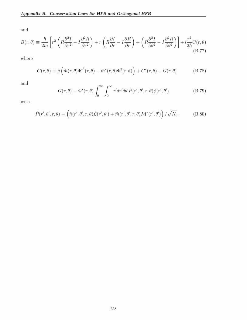
Appendix B. Conservation Laws for HFB and Orthogonal HFB
and
B(r, θ) ≡ ~
2m
[
r2
(
R∂2I
∂r2− I ∂
2R
∂r2
)
+ r
(
R∂I
∂r− I ∂R
∂r
)
+
(
R∂2I
∂θ2− I ∂
2R
∂θ2
)]
+ ir2
2~C(r, θ)
(B.77)
where
C(r, θ) ≡ g(
m(r, θ)Φ∗2
(r, θ)− m∗(r, θ)Φ2(r, θ))
+G∗(r, θ)−G(r, θ) (B.78)
and
G(r, θ) ≡ Φ∗(r, θ)
∫ 2π
0
∫ ∞
0
r′dr′dθ′P (r′, θ′, r, θ)φ(r′, θ′) (B.79)
with
P (r′, θ′, r, θ) =(
n(r′, θ′, r, θ)L(r′, θ′) + m(r′, θ′, r, θ)M∗(r′, θ′))
/√
Nc. (B.80)
258
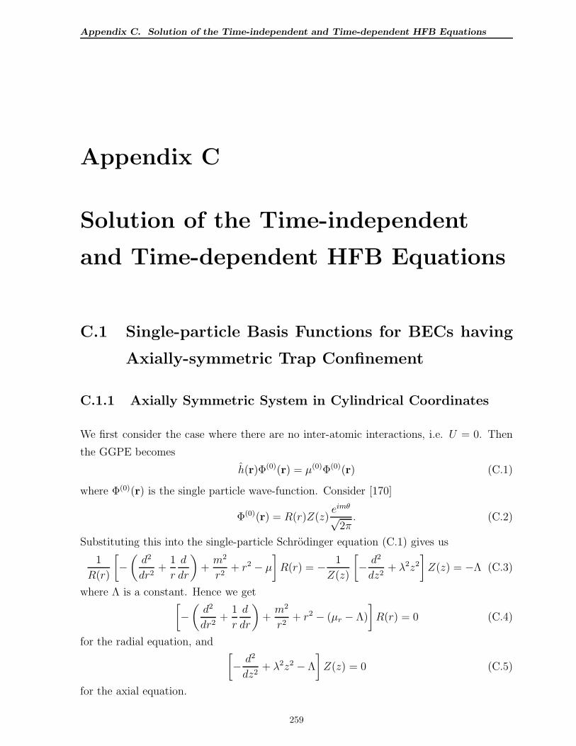
Appendix C. Solution of the Time-independent and Time-dependent HFB Equations
Appendix C
Solution of the Time-independent
and Time-dependent HFB Equations
C.1 Single-particle Basis Functions for BECs having
Axially-symmetric Trap Confinement
C.1.1 Axially Symmetric System in Cylindrical Coordinates
We first consider the case where there are no inter-atomic interactions, i.e. U = 0. Then
the GGPE becomes
h(r)Φ(0)(r) = µ(0)Φ(0)(r) (C.1)
where Φ(0)(r) is the single particle wave-function. Consider [170]
Φ(0)(r) = R(r)Z(z)eimθ
√2π. (C.2)
Substituting this into the single-particle Schrodinger equation (C.1) gives us
1
R(r)
[
−(
d2
dr2+
1
r
d
dr
)
+m2
r2+ r2 − µ
]
R(r) = − 1
Z(z)
[
− d2
dz2+ λ2z2
]
Z(z) = −Λ (C.3)
where Λ is a constant. Hence we get[
−(
d2
dr2+
1
r
d
dr
)
+m2
r2+ r2 − (µr − Λ)
]
R(r) = 0 (C.4)
for the radial equation, and[
− d2
dz2+ λ2z2 − Λ
]
Z(z) = 0 (C.5)
for the axial equation.
259
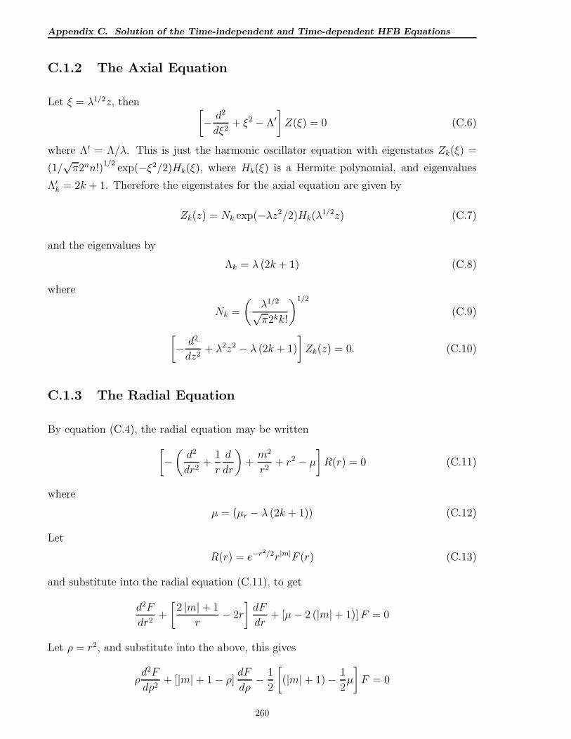
Appendix C. Solution of the Time-independent and Time-dependent HFB Equations
C.1.2 The Axial Equation
Let ξ = λ1/2z, then[
− d2
dξ2+ ξ2 − Λ′
]
Z(ξ) = 0 (C.6)
where Λ′ = Λ/λ. This is just the harmonic oscillator equation with eigenstates Zk(ξ) =
(1/√π2nn!)
1/2exp(−ξ2/2)Hk(ξ), where Hk(ξ) is a Hermite polynomial, and eigenvalues
Λ′k = 2k + 1. Therefore the eigenstates for the axial equation are given by
Zk(z) = Nk exp(−λz2/2)Hk(λ1/2z) (C.7)
and the eigenvalues by
Λk = λ (2k + 1) (C.8)
where
Nk =
(
λ1/2
√π2kk!
)1/2
(C.9)
[
− d2
dz2+ λ2z2 − λ (2k + 1)
]
Zk(z) = 0. (C.10)
C.1.3 The Radial Equation
By equation (C.4), the radial equation may be written
[
−(
d2
dr2+
1
r
d
dr
)
+m2
r2+ r2 − µ
]
R(r) = 0 (C.11)
where
µ = (µr − λ (2k + 1)) (C.12)
Let
R(r) = e−r2/2r|m|F (r) (C.13)
and substitute into the radial equation (C.11), to get
d2F
dr2+
[
2 |m|+ 1
r− 2r
]
dF
dr+ [µ− 2 (|m|+ 1)]F = 0
Let ρ = r2, and substitute into the above, this gives
ρd2F
dρ2+ [|m|+ 1− ρ] dF
dρ− 1
2
[
(|m|+ 1)− 1
2µ
]
F = 0
260
Appendix C. Solution of the Time-independent and Time-dependent HFB Equations
In order to render the solution physical, we require that the quantity −12
[
(|m| + 1)− 12µ]
be an integer, n, say, i.e.
n = −1
2
[
(|m|+ 1)− 1
2µ
]
.
Then
ρd2F
dρ2+ [|m|+ 1− ρ] dF
dρ+ nF = 0
which is in the form of the associated Laguerre differential equation, so we may write
F (ρ) = N |m|n L|m|
n (ρ)
where L|m|n (ρ) is an associated Laguerre polynomial. Hence the radial equation has eigen-
states given by
R|m|n (r) = N |m|
n e−r2/2r|m|L|m|n (r2) (C.14)
with eigenvalues
µ = 2 (2n+ 1 + |m|) (C.15)
where
N |m|n =
(
2n!
(n+ |m|)!
)1/2
(C.16)
is the normalisation constant, i.e.
[
−(
d2
dr2+
1
r
d
dr
)
+m2
r2+ r2 − 2 (2n+ 1 + |m|)
]
R|m|n (r) = 0. (C.17)
The chemical potential µr is given by
µr = 2 (2n+ 1 + |m|) + λ (2k + 1) . (C.18)
C.1.4 Single Particle Eigenstates
The single particle eigenstates may therefore be written as
Φ(0)nkm(r) = R|m|
n (r)Zk(z)eimθ
√2π
(C.19)
with eigenvalue
µnkm = 2 (2n+ 1 + |m|) + λ (2k + 1) . (C.20)
Alternatively, defining the Laguerre basis functions
ξmn(r, θ) =
(
n!
π(n+ |m|)!
)1/2
eimθe−r2/2r|m|L|m|n (r2) =
eimθ
√2πR|m|
n (r) (C.21)
261
Appendix C. Solution of the Time-independent and Time-dependent HFB Equations
we may also write the single particle eigenstates in the form
Φ(0)nkm(r) = ξmn(r, θ)Zk(z). (C.22)
The motivation for defining the Laguerre basis functions ξm,n(r, θ) is that they form an
orthonormal set, i.e.
∫ 2π
0
∫ ∞
0
rdrdθξ∗mn(r, θ)ξm′n′(r, θ) = δn,n′δm,m′ (C.23)
whereas the functions
R|m|n (r)
are only orthogonal for a given value of the quantum
number m, i.e.∫ ∞
0
rdrR|m|n (r)R
|m|n′ (r) = δn,n′ (C.24)
but∫ ∞
0
rdrR|m|n (r)R
|m′|n′ (r) 6= δn,n′δm,m′ . (C.25)
C.1.5 The Hermite and Laguerre Basis Functions
The Hermite Basis Set
We use the notation ζk(z) ≡ Zk(z) for the set of eigenstates satisfying (C.6) and refer
to the set of basis functions ζk(z), k = 0, . . . , K as the Hermite single particle basis
corresponding to a computational mode cut-off of k = 0, . . . , K.
The Laguerre Basis Set
We use the notation ξln(r) ≡ R|l|n (r) to represent the radial Laguerre function with principle
quantum number n, and angular quantum number l satisfying the the radial equation
(C.17), and rewrite ξln(r, θ) given by (C.21) in the form
ξln(r, θ) =eilθ
√2πξln(r), (C.26)
where
ξln(r) =
(
2n!
(n+ |l|)!
)1/2
e−r2/2r|l|L|l|n (r2). (C.27)
We refer to the set of basis functions
ξln(r, θ), n = 0, . . . , N, l = 0,±1, . . . ,±L
262
Appendix C. Solution of the Time-independent and Time-dependent HFB Equations
as the Laguerre single particle basis corresponding to a computational mode cut-off of n =
0, . . . , N and l = 0,±1, . . . ,±L. In the 2D case where the axial confinement is sufficiently
strong that we can neglect all axial states other than the lowest energy state, i.e., we can
restrict ourselves to k = 0, we integrate out the axial coordinate z . We generally absorb the
energy term of λ harmonic energy units ~ωr/2 in the expression µn0l = 2 (2n+ 1 + |l|) +
λ into the system chemical potential µ and write the single particle eigenvalue energies
corresponding to the Laguerre basis functions as µ(SP )ln = 2 (2n + 1 + |l|).
C.2 Time-independent HFB Equations
C.2.1 General Method of Solution for BECs in Axially Symmet-
ric Harmonic Trap using Single Particle Basis Functions
We expand the condensate wave-function Φ(r) and the quasi-particle amplitudes uq(r) and
vq(r) in terms of the single-particle basis functions ξk(r) = ξln(r, θ)ζk(z). These single-
particle basis functions are solutions of the (single-particle) time-independent Schrodinger
equation with respective energy eigenvalues µ(SP )k , viz.
µ(SP )k ξk(r) = h(r)ξk(r). (C.28)
Thus we may write the condensate wave function Φ(r) as
Φ(r) =∑
k
a0kξk(r) (C.29)
and the quasiparticle amplitudes uq(r) and vq(r) as
uq(r) =∑
k
cqkξk(r) (C.30)
and
vq(r) =∑
k
dqkξk(r) (C.31)
respectively. We substitute (C.29) into the dimensionless modified GGPE (5.20), i.e.
µΦ(r) =(
h(r) + C3D
(
|Φ(r)|2 + 2n(r))
)
Φ(r)+C3Dm(r)Φ∗(r)−∫
dr′P (r′, r)φ(r′) (C.32)
where we have neglected ∆µ, which we showed to be negligible in Chapter 4. In this
way we obtain the matrix (eigenvalue) equation for the coefficients ak for the condensate
263
Appendix C. Solution of the Time-independent and Time-dependent HFB Equations
wave-function Φ(r) given by
µak =∑
k′
(Ak,k′ +Bk,k′) ak′ (C.33)
written in terms of the matrix elements
Ak,k′ ≡ µ(SP )k,Ω δk,k′ + C3D
∫
drξ∗k(r)(
|Φ(r)|2 + 2n(r))
ξk′(r)− Pk,k′ (C.34)
and
Bk,k′ ≡ C3D
∫
drξ∗k(r)m(r)ξ∗k′(r) (C.35)
where
Pk,k′ =∫
drdr′ξ∗k(r)[
n(r′, r)(
µ(SP )k′,Ω − µ+ 2C3D
(
|Φ(r′)|2 + n(r′))
)
+C3Dm(r′, r)(
Φ∗2(r′) + m∗(r′)
)]
ξk′(r′)/Nc.(C.36)
Note that we use lowest energy eigenvector for condensate wave-function, and hence the
coefficients a0k. Similarly we substitute (C.30) and (C.31) into the dimensionless orthogonal
BdGEs (5.21)
ǫq
[
uq(r)
vq(r)
]
=∫
dr′
[
L(r, r′) M(r, r′)
−M∗(r, r′) −L∗(r, r′)
][
uq(r′)
vq(r′)
]
(C.37)
where, as before
L(r, r′) ≡ Q(r, r′)L(r′)
M(r, r′) ≡ Q(r, r′)M(r′)(C.38)
withL(r) ≡ h(r)− µ+ 2C3D
(
|Φ(r)|2 + n(r))
M(r) ≡ C3D (Φ2(r) + m(r))(C.39)
to obtain matrix (eigenvalue) equations for the coefficients cqk and dqk for the quasi-particle
amplitudes uq(r) and vq(r)
ǫq
[
cqk
dqk
]
=∑
k′
[
L(u)q,k,k′ M
(u)q,k,k′
−M (v)q,k,k′ −L(v)
q,k,k′
][
cqk′
dqk′
]
(C.40)
written in terms of the respective matrix elements
L(u)q,k,k′ ≡
(
µ(SP )k − µ
)
(
δk,k′ − 1
Nc
I(1)k I
(1)∗
k′
)
+ I(u)q,k,k′, (C.41)
L(v)q,k,k′ ≡
(
µ(SP )k − µ
)
(
δk,k′ − 1
NcI
(2)k I
(2)∗
k′
)
+ I(v)q,k,k′, (C.42)
264
Appendix C. Solution of the Time-independent and Time-dependent HFB Equations
M(u)q,k,k′ ≡ C3D
∫
dr
(
ξ∗k(r)−1
NcI
(1)k Φ∗(r)
)
(
Φ2(r) + m(r))
ξk′(r), (C.43)
M(v)q,k,k′ ≡ C3D
∫
dr
(
ξ∗k(r)−1
NcI
(2)k Φ(r)
)
(
Φ∗2
(r) + m∗(r))
ξk′(r), (C.44)
where
I(u)q,k,k′ ≡ 2C3D
∫
dr
(
ξ∗k(r)−1
NcI
(1)k Φ∗(r)
)
(
|Φ(r)|2 + n(r))
ξk′(r), (C.45)
I(v)q,k,k′ ≡ 2C3D
∫
dr
(
ξ∗k(r)−1
NcI
(2)k Φ(r)
)
(
|Φ(r)|2 + n(r))
ξk′(r), (C.46)
I(1)k ≡
∫
drξ∗k(r)Φ(r), (C.47)
and
I(2)k ≡
∫
drξ∗k(r)Φ∗(r). (C.48)
Defining the vectors a, cq, and dq corresponding to the coefficients ak, cq,k, and dq,k, and the
matrices A, B, L(u)q , M
(u)q , L
(v)q , and M
(v)q corresponding to the matrix elements Ak,k′, Bk,k′,
L(u)q,k,k′, M
(u)q,k,k′, L
(v)q,k,k′, and M
(v)q,k,k′ respectively, we obtain the following matrix equations:
The coefficients for the condensate wavefunction (GGPE) and the chemical potential are
obtained by solving the matrix eigenvalue equation
µa = (A + B)a. (C.49)
On the other hand, the coefficients for the quasiparticle amplitudes and the quasi-particle
energies are obtained by solving the matrix eigenvalue equation
ǫq
[
cq
dq
]
=
[
L(u)q M
(u)q
−M(v)q −L
(v)q
][
cq
dq
]
(C.50)
corresponding to the BdGEs. In the laboratory (LAB) frame in the axially symmetric case
and in the absence of any vortices, we have L(u)q = L
(v)q and M
(u)q = M
(v)q , but this is not
the case in general.
We generally neglect the projection part∫
dr′P (r′, r)φ(r′) in the time-independent solu-
tions for the GGPE since results (not presented here) indicate that the effect is small
and implies an unnecessary increase in the computational effort in solving the orthogonal
HFB equations. The projection part was included in some of the solutions, the effect of
its inclusion having a negligible effect on the time-independent solution. The projection
part is however crucially important in the time-dependent formalism in the conservation
of angular and linear momentum.
265
Appendix C. Solution of the Time-independent and Time-dependent HFB Equations
C.2.2 Solutions for Quasi-2D BEC in Axially-symmetric Trap -
Axially-symmetric Solutions
In the case of axial symmetry of the solutions, we can integrate out the azimuthal coordinate
θ to obtain the radial time-independent orthogonal HFB equations comprised of the radial
time-independent GGPE (7.14)
µΦ(r) =(
hm(r)− µ+ CR2D
(
|Φ(r)|2 + 2n(r))
)
Φ(r)+CR2Dm(r)Φ(r)−
∫ ∞
0
r′dr′P (r′, r)φ(r′)
(C.51)
and the radial time-independent orthogonal BdGEs (7.15)
ǫlq
[
ulq(r)
vlq(r)
]
=∫∞0r′dr′
[
Ql(r, r′)Ll+m(r′) Ql(r, r
′)M(r′)
−Ql(r, r′)M(r′) −Ql(r, r
′)Ll−m(r′)
][
ulq(r′)
vlq(r′)
]
(C.52)
(see sections 5.3.1 and 7.2). In this case we can expand the radial condensate wave-
function Φ(r) and the radial quasi-particle amplitudes ulq(r) and vlq(r) in terms of the
radial Laguerre basis functions ξln(r), i.e.
Φ(r) =∑
n
anξmn(r) (C.53)
for the condensate wave-function, and
uq(r) =∑
l,n
cq,lnξl+m,n(r) (C.54)
and
vq(r) =∑
l,n
dq,lnξl−m,n(r) (C.55)
for the quasi-particle amplitudes. Here we have allowed for the existence of an on-axis
vortex of vorticity m . In the case of no vortices, m = 0. Substituting (C.53) into the
GGPE (C.51), and (C.54),(C.55) into the orthogonal BdGEs (C.52), we find that
µan =∑
n′
An,n′an′ (C.56)
and
ǫq,l
[
cq,ln
dq,ln
]
=∑
n′
[
L(u)q,l,n,n′ M
(u)q,l,n,n′
−M (v)q,l,n,n′ −L(v)
q,l,n,n′
][
cq,l′n′
dq,l′n′
]
(C.57)
where we have defined
An,n′ ≡(
µ(SP )mn −mΩ
)
δn,n′ + CR2D
∞∫
0
rdrξmn(r)(
|Φ(r)|2 + 2n(r) + m(r))
ξmn′(r)− Pn,n′
(C.58)
266
Appendix C. Solution of the Time-independent and Time-dependent HFB Equations
with
Pn,n′ =∫∞0
∫∞0rdrr′dr′ξmn(r)
[
n(r′, r)(
µ(SP )mn −mΩ− µ+ 2CR
2D
(
|Φ(r′)|2 + n(r′))
)
+CR2Dm(r′, r) (Φ2(r′) + m(r′))
]
ξmn′(r′)/Nc,
(C.59)
and
L(u)q,l,n,n′ ≡
(
µ(SP )ln − (l +m)Ω− µ
)
(
δl,l′δn,n′ − δl,0Nc
I(1)l+m,nI
(1)l+m,n′
)
+ I(u)q,l,n,n′, (C.60)
L(v)q,l,n,n′ ≡
(
µ(SP )ln + (l −m)Ω− µ
)
(
δl,l′δn,n′ − δl,0Nc
I(2)l−m,nI
(2)l−m,n′
)
+ I(v)q,l,n,n′, (C.61)
M(u)q,l,n,n′ ≡ CR
2D
∞∫
0
rdr
(
ξl+m,n(r)−δl,0Nc
I(1)l+m,nΦ(r)
)
(
Φ2(r) + m(r))
ξl−m,n′(r), (C.62)
M(v)q,l,n,n′ ≡ CR
2D
∞∫
0
rdr
(
ξl−m,n(r)−δl,0Nc
I(2)l−m,nΦ(r)
)
(
Φ2(r) + m(r))
ξl+m,n′(r), (C.63)
where
I(u)q,l,n,n′ ≡ 2CR
2D
∞∫
0
rdr
(
ξl+m,n(r)−δl,0Nc
I(1)l+m,nΦ(r)
)
(
|Φ(r)|2 + n(r))
ξl+m,n′(r), (C.64)
I(v)q,l,n,n′ ≡ 2CR
2D
∞∫
0
rdr
(
ξl−m,n(r)−δl,0Nc
I(2)l−m,nΦ(r)
)
(
|Φ(r)|2 + n(r))
ξl−m,n′(r), (C.65)
and
I(1)ln = I
(2)ln =
∞∫
0
rdrξln(r)Φ(r). (C.66)
Defining the vectors a, cq,l and dq,l corresponding to the coefficients an, cq,lnand dq,ln, and
the matrices A, B, L(u)q,l , M
(u)q,l , L
(v)q,l and M
(v)q,l corresponding to the matrix elements An,n′,
Bn,n′, L(u)q,l,n,n′, M
(u)q,l,n,n′, L
(v)q,l,n,n′ and M
(v)q,l,n,n′, we obtain the matrix eigenvalue equation for
the coefficients for the condensate wavefunction (GGPE)
µa = Aa (C.67)
and for the quasi-particle amplitudes (BdGEs)
ǫq,l
[
cq,l
dq,l
]
=
[
L(u)q,l M
(u)q,l
−M(v)q,l −L
(v)q,l
][
cq,l
dq,l
]
. (C.68)
We note that the radial Laguerre basis functions ξln(r) given by equation (C.27) may
be written as a polynomial of order n + l in r2 times a weighting factor exp (−r2/2),
267
Appendix C. Solution of the Time-independent and Time-dependent HFB Equations
thus all matrix elements are integrals of orthogonal polynomials of order 4N + 2M − 4
in r2 (since dr2 = 2rdr), where we have imposed the computational mode cut-off of
n = 0, . . . , N − 1 and l = 0,±1, . . . ,±M . This facilitates the use of Gaussian quadra-
ture for the integration (see section 5.5 in chapter 5 on numerical methods), allowing accu-
rate computation for a minimal number of position points, greatly enhancing the efficiency
and accuracy of the numerical algorithms used here.
C.2.3 Solutions for 2D BEC in Axially-symmetric trap - General
Case
We consider the numerical solution for the dimensionless time-independent HFB equations
(5.36) and (5.37) in the 2D case (pancake BEC) in the case where no assumptions are made
concerning the axial symmetry of the solutions, in the case of no vortices, and in the case
of off-axis vortices.
No Vortices
We expand the condensate wavefunction Φ(r, θ) and quasiparticle amplitudes uq(r, θ),
vq(r, θ) in the Laguerre basis
ξln(r, θ), l = 0,±1, . . . , n = 0, 1, . . .
where the ξln(r, θ)
are given by (C.26) and (C.27)
ξln(r, θ) =eilθ
√2π
(
2n!
(n+ |l|)!
)1/2
e−r2/2r|l|L|l|n (r2) = ξln(r)
eilθ
√2π,
Φ(r, θ) =∑
ln
a0,lnξln(r, θ) (C.69)
uq(r, θ) =∑
ln
cq,lnξln(r, θ) (C.70)
and
vq(r, θ) =∑
ln
dq,lnξln(r, θ). (C.71)
Substituting (C.69) into the GGPE (5.36), and (C.70),(C.71) into the orthogonal BdGEs
(5.37), we find that
µaln =∑
l′n′
(Aln,l′n′ +Bln,l′n′) al′n′ (C.72)
and
ǫq
[
cq,ln
dq,ln
]
=∑
l′n′
[
L(u)q,ln,l′n′ M
(u)q,ln,l′n′
−M (v)q,ln,l′n′ −L(v)
q,ln,l′n′
][
cq,l′n′
dq,l′n′
]
(C.73)
268
Appendix C. Solution of the Time-independent and Time-dependent HFB Equations
where we have defined
Aln,l′n′ ≡(
µ(SP )ln − lΩ
)
δl,l′δn,n′+C2D
∞∫
0
2π∫
0
rdrdθξ∗ln(r, θ)(
|Φ(r, θ)|2 + 2n(r, θ))
ξl′n′(r, θ)−Pln,l′n′,
(C.74)
Pln,l′n′ ≡∫∞0
∫ 2π
0
∫∞0
∫ 2π
0rdrdθr′dr′dθ′ξ∗ln(r, θ) [
n(r′, θ′, r, θ)(
µ(SP )l′n′ − l′Ω− µ+ 2C2D
(
|Φ(r′, θ′)|2 + n(r′, θ′))
)
+C2Dm(r′, θ′, r, θ)(
Φ∗2(r′, θ′) + m∗(r′, θ′)
)]
ξl′n′(r′, θ′)/Nc,
(C.75)
Bln,l′n′ ≡ C2D
∞∫
0
2π∫
0
rdrdθξ∗ln(r, θ)m(r, θ)ξ∗l′n′(r, θ), (C.76)
L(u)q,ln,l′n′ ≡
(
µ(SP )ln − lΩ− µ
)
(
δl,l′δn,n′ − 1
Nc
I(1)ln I
(1)∗
l′n′
)
+ I(u)q,ln,l′n′, (C.77)
L(v)q,ln,l′n′ ≡
(
µ(SP )ln + lΩ− µ
)
(
δl,l′δn,n′ − 1
NcI
(2)ln I
(2)∗
l′n′
)
+ I(v)q,ln,l′n′, (C.78)
M(u)q,ln,l′n′ ≡ C2D
∞∫
0
2π∫
0
rdrdθ
(
ξ∗ln(r, θ)−1
NcI
(1)ln Φ∗(r, θ)
)
(
Φ2(r, θ) + m(r, θ))
ξl′n′(r, θ),
(C.79)
M(v)q,ln,l′n′ ≡ C2D
∞∫
0
2π∫
0
rdrdθ
(
ξ∗ln(r, θ)− 1
Nc
I(2)ln Φ(r, θ)
)
(
Φ∗2
(r, θ) + m∗(r, θ))
ξl′n′(r, θ),
(C.80)
where
I(u)q,ln,l′n′ ≡ 2C2D
∞∫
0
2π∫
0
rdrdθ
(
ξ∗ln(r, θ)− 1
NcI
(1)ln Φ∗(r, θ)
)
(
|Φ(r, θ)|2 + n(r, θ))
ξl′n′(r, θ),
(C.81)
I(v)q,ln,l′n′ ≡ 2C2D
∞∫
0
2π∫
0
rdrdθ
(
ξ∗ln(r, θ)−1
NcI
(2)ln Φ(r, θ)
)
(
|Φ(r, θ)|2 + n(r, θ))
ξl′n′(r, θ),
(C.82)
I(1)ln ≡
∞∫
0
2π∫
0
rdrdθξ∗ln(r, θ)Φ(r, θ) (C.83)
I(2)ln ≡
∞∫
0
2π∫
0
rdrdθξ∗ln(r, θ)Φ∗(r, θ). (C.84)
Defining the vectors a, cq and dq corresponding to the coefficients aln, cq,lnand dq,ln, and
the matrices A, B, L(u)q , M
(u)q , L
(v)q and M
(v)q corresponding to the matrix elements Aln,l′n′,
269
Appendix C. Solution of the Time-independent and Time-dependent HFB Equations
Bln,l′n′, L(u)q,l,n,l′,n′, M
(u)q,l,n,l′,n′, L
(v)q,l,n,l′,n′ and M
(v)q,l,n,l′,n′, we obtain the vector eigenvalue equa-
tion for the coefficients for the condensate wavefunction (GGPE)
µa = (A + B)a (C.85)
and for the quasiparticle amplitudes (BdGEs)
ǫq
[
cq
dq
]
=
[
L(u)q M
(u)q
−M(v)q −L
(v)q
][
cq
dq
]
. (C.86)
Off-axis Vortices
We find stationary solutions for a single off-axis vortex by solving the 2D HFB equations
(5.36) and (5.37) and the equation for the precessional frequency (4.65) self-consistently,
with C(r, θ) given by (4.125). We can write the condensate wave function Φ(r, θ) in terms
of the modified single-particle basis
χ(1)ln (r, θ), (l, n) ∈ S(1)
for a single vortex where we
have defined (5.63)
S(1) ≡ l, n | (l, n) ∈ S − (1, 0) (C.87)
with the definition S ≡ l, n | n = 0, . . . , l = 0,±1, . . . as (5.64)
Φ(r, θ) =∑
l,n∈S(1)
alnχ(1)ln (r, θ) (C.88)
where (5.65)
χ(1)ln (r, θ) ≡ ξln(r, θ)−
ξln(rNv, θNv
)
ξ10(rNv, θNv
)ξ10(r, θ). (C.89)
For multiple off-axis vortices we write the condensate wave function Φ(r, θ) in terms of the
modified single-particle basis
χ(Nv)ln (r, θ), (l, n) ∈ S(Nv)
for Nv off-axis vortices situated
at positions (r, θ) ∈ (ri, θi) | i = 1, . . . Nv as (5.69)
Φ(r, θ) =∑
l,n∈S(Nv)
alnχ(Nv)ln (r, θ) (C.90)
where we have defined (5.67)
S(Nv) ≡ l, n | (l, n) ∈ S − (1, 0) , . . . , (Nv, 0) , (C.91)
and where the modified basis functions are given by (5.70)
χ(Nv)ln (r, θ) ≡ χ
(Nv−1)ln (r, θ)− χ
(Nv−1)ln (rNv
, θNv)
χ(Nv−1)Nv0 (rNv
, θNv)χ
(Nv−1)Nv0 (r, θ). (C.92)
270
Appendix C. Solution of the Time-independent and Time-dependent HFB Equations
As before, we expand the quasiparticle amplitudes uq(r, θ), vq(r, θ) in the Laguerre basis
ξln(r, θ), l = 0,±1, . . . , n = 0, 1, . . .
(see (C.70),(C.71))
uq(r, θ) =∑
l,n
cq,lnξln(r, θ) (C.93)
and
vq(r, θ) =∑
l,n
dq,lnξln(r, θ) (C.94)
Substituting (C.90) into the GGPE (5.36), and (C.93),(C.94) into the orthogonal BdGEs
(5.37), we find that
µaln =∑
l′,n′∈S(1)
(Aln,l′n′ +Bln,l′n′) al′n′ (C.95)
and
ǫq
[
cq,ln
dq,ln
]
=∑
l′n′
[
L(u)q,ln,l′n′ M
(u)q,ln,l′n′
−M (v)q,ln,l′n′ −L(v)
q,ln,l′n′
][
cq,l′n′
dq,l′n′
]
(C.96)
where we have defined
Aln,l′n′ ≡(
µ(SP )ln − lΩ
)
δl,l′δn,n′+C2D
∞∫
0
2π∫
0
rdrdθξ∗ln(r, θ)(
|Φ(r, θ)|2 + 2n(r, θ))
χ(Nv)l′n′ (r, θ)−Pln,l′n′,
(C.97)
Pln,l′n′ ≡∫∞0
∫ 2π
0
∫∞0
∫ 2π
0rdrdθr′dr′dθ′ξ∗ln(r, θ) [
n(r′, θ′, r, θ)(
µ(SP )l′n′ − l′Ω− µ+ 2C2D
(
|Φ(r′, θ′)|2 + n(r′, θ′))
)
+C2Dm(r′, θ′, r, θ)(
Φ∗2(r′, θ′) + m∗(r′, θ′)
)]
χ(Nv)l′n′ (r′, θ′)/Nc,
(C.98)
Bln,l′n′ ≡ C2D
∞∫
0
2π∫
0
rdrdθξ∗ln(r, θ)m(r, θ)χ(Nv)∗
l′n′ (r, θ), (C.99)
L(u)q,ln,l′n′ ≡
(
µ(SP )ln − lΩ− µ
)
(
δl,l′δn,n′ − 1
NcI
(1)ln I
(1)∗
l′n′
)
+ I(u)q,ln,l′n′, (C.100)
L(v)q,ln,l′n′ ≡
(
µ(SP )ln + lΩ− µ
)
(
δl,l′δn,n′ − 1
Nc
I(2)ln I
(2)∗
l′n′
)
+ I(v)q,ln,l′n′, (C.101)
M(u)q,ln,l′n′ ≡ C2D
∞∫
0
2π∫
0
rdrdθ
(
ξ∗ln(r, θ)−1
NcI
(1)ln Φ∗(r, θ)
)
(
Φ2(r, θ) + m(r, θ))
ξl′n′(r, θ),
(C.102)
M(v)q,ln,l′n′ ≡ C2D
∞∫
0
2π∫
0
rdrdθ
(
ξ∗ln(r, θ)− 1
Nc
I(2)ln Φ(r, θ)
)
(
Φ∗2
(r, θ) + m∗(r, θ))
ξl′n′(r, θ),
(C.103)
271
Appendix C. Solution of the Time-independent and Time-dependent HFB Equations
where
I(u)q,ln,l′n′ ≡ 2C2D
∞∫
0
2π∫
0
rdrdθ
(
ξ∗ln(r, θ)−1
NcI
(1)ln Φ∗(r, θ)
)
(
|Φ(r, θ)|2 + n(r, θ))
ξl′n′(r, θ),
(C.104)
I(v)q,ln,l′n′ ≡ 2C2D
∞∫
0
2π∫
0
rdrdθ
(
ξ∗ln(r, θ)− 1
NcI
(2)ln Φ(r, θ)
)
(
|Φ(r, θ)|2 + n(r, θ))
ξl′n′(r, θ),
(C.105)
I(1)ln ≡
∞∫
0
2π∫
0
rdrdθξ∗ln(r, θ)Φ(r, θ), (C.106)
and
I(2)ln ≡
∞∫
0
2π∫
0
rdrdθξ∗ln(r, θ)Φ∗(r, θ). (C.107)
Defining the vectors a, cq,l and dq,l corresponding to the coefficients aln, cq,lnand dq,ln,
and the matrices A, B, L(u)q , M
(u)q , L
(v)q and M
(v)q corresponding to the matrix elements
Aln,l′n′, Bln,l′n′ , L(u)q,l,n,l′,n′, M
(u)q,l,n,l′,n′, L
(v)q,l,n,l′,n′ and M
(v)q,l,n,l′,n′, we obtain the vector eigenvalue
equation for the coefficients for the condensate wavefunction (GGPE)
µa = (A + B)a (C.108)
and for the quasiparticle amplitudes (BdGEs)
ǫq
[
cq
dq
]
=
[
L(u)q M
(u)q
−M(v)q −L
(v)q
][
cq
dq
]
. (C.109)
C.2.4 Numerical Calculation of the Precessional Frequency Ω for
the Off-Axis Case
We use equation (4.65)
Ω =
∫ 2π
0
∫∞0A(r, θ)B(r, θ)rdrdθ
∫ 2π
0
∫∞0
(A(r, θ))2 rdrdθ(C.110)
to calculate the precessional frequency Ω in the case of single and multiple off-axis vortices.
Here we have defined (4.62)
A(r, θ) ≡(
R∂R
∂θ+ I
∂I
∂θ
)
(C.111)
272
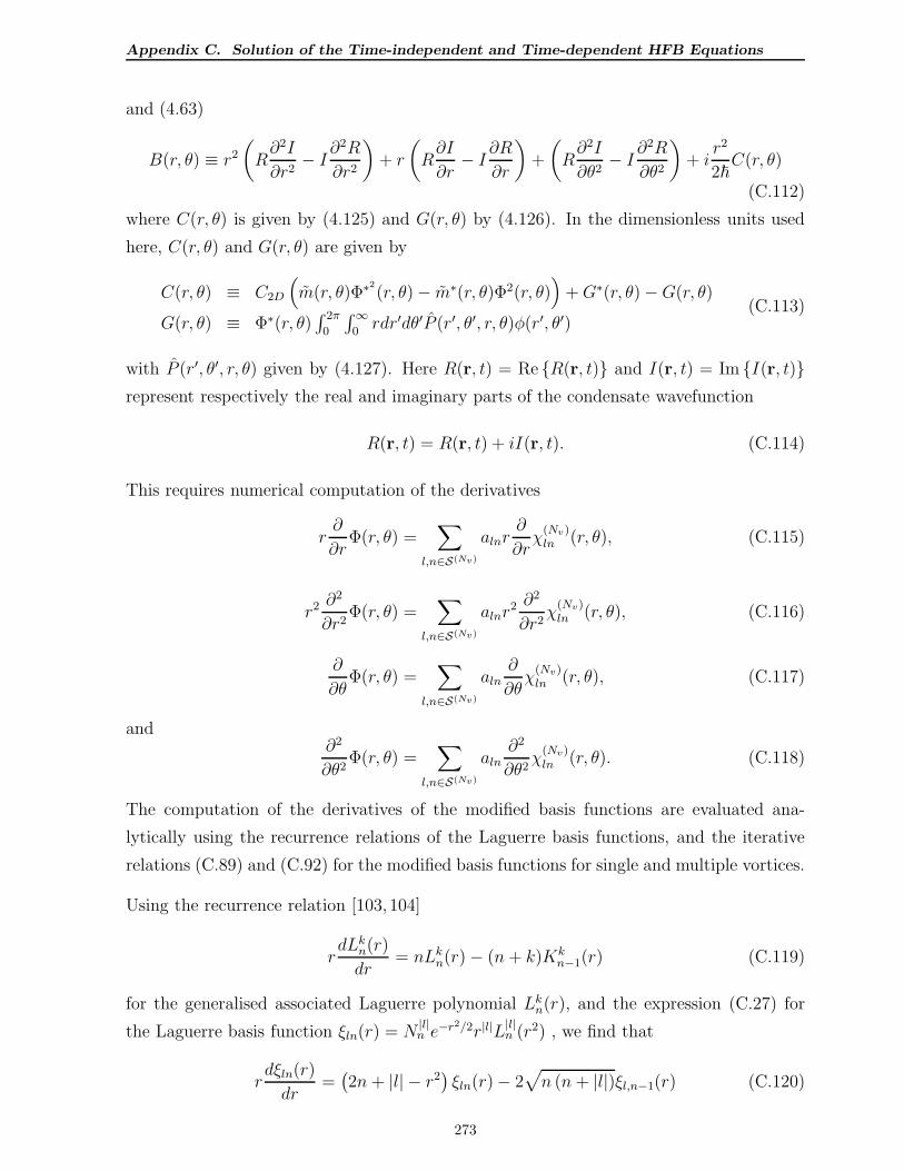
Appendix C. Solution of the Time-independent and Time-dependent HFB Equations
and (4.63)
B(r, θ) ≡ r2
(
R∂2I
∂r2− I ∂
2R
∂r2
)
+ r
(
R∂I
∂r− I ∂R
∂r
)
+
(
R∂2I
∂θ2− I ∂
2R
∂θ2
)
+ ir2
2~C(r, θ)
(C.112)
where C(r, θ) is given by (4.125) and G(r, θ) by (4.126). In the dimensionless units used
here, C(r, θ) and G(r, θ) are given by
C(r, θ) ≡ C2D
(
m(r, θ)Φ∗2(r, θ)− m∗(r, θ)Φ2(r, θ)
)
+G∗(r, θ)−G(r, θ)
G(r, θ) ≡ Φ∗(r, θ)∫ 2π
0
∫∞0rdr′dθ′P (r′, θ′, r, θ)φ(r′, θ′)
(C.113)
with P (r′, θ′, r, θ) given by (4.127). Here R(r, t) = Re R(r, t) and I(r, t) = Im I(r, t)represent respectively the real and imaginary parts of the condensate wavefunction
R(r, t) = R(r, t) + iI(r, t). (C.114)
This requires numerical computation of the derivatives
r∂
∂rΦ(r, θ) =
∑
l,n∈S(Nv)
alnr∂
∂rχ
(Nv)ln (r, θ), (C.115)
r2 ∂2
∂r2Φ(r, θ) =
∑
l,n∈S(Nv)
alnr2 ∂
2
∂r2χ
(Nv)ln (r, θ), (C.116)
∂
∂θΦ(r, θ) =
∑
l,n∈S(Nv)
aln∂
∂θχ
(Nv)ln (r, θ), (C.117)
and∂2
∂θ2Φ(r, θ) =
∑
l,n∈S(Nv)
aln∂2
∂θ2χ
(Nv)ln (r, θ). (C.118)
The computation of the derivatives of the modified basis functions are evaluated ana-
lytically using the recurrence relations of the Laguerre basis functions, and the iterative
relations (C.89) and (C.92) for the modified basis functions for single and multiple vortices.
Using the recurrence relation [103,104]
rdLk
n(r)
dr= nLk
n(r)− (n+ k)Kkn−1(r) (C.119)
for the generalised associated Laguerre polynomial Lkn(r), and the expression (C.27) for
the Laguerre basis function ξln(r) = N|l|n e−r2/2r|l|L
|l|n (r2) , we find that
rdξln(r)
dr=(
2n + |l| − r2)
ξln(r)− 2√
n (n + |l|)ξl,n−1(r) (C.120)
273
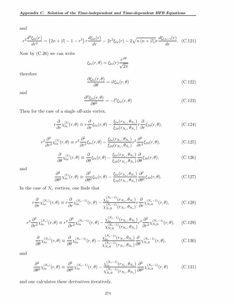
Appendix C. Solution of the Time-independent and Time-dependent HFB Equations
and
r2d2ξln(r)
dr2=(
2n+ |l| − 1− r2)
rdξln(r)
dr− 2r2ξln(r)− 2
√
n (n + |l|)rdξl,n−1(r)
dr. (C.121)
Now by (C.26) we can write
ξln(r, θ) = ξln(r)eilθ
√2π
therefore∂ξln(r, θ)
∂θ= ilξln(r, θ) (C.122)
and∂2ξln(r, θ)
∂θ2= −l2ξln(r, θ) (C.123)
Then for the case of a single off-axis vortex,
r∂
∂rχ
(1)ln (r, θ) ≡ r
∂
∂rξln(r, θ)− ξln(rNv
, θNv)
ξ10(rNv, θNv
)r∂
∂rξ10(r, θ), (C.124)
r2 ∂2
∂r2χ
(1)ln (r, θ) ≡ r2 ∂
2
∂r2ξln(r, θ)−
ξln(rNv, θNv
)
ξ10(rNv, θNv
)r2 ∂
2
∂r2ξ10(r, θ), (C.125)
∂
∂θχ
(1)ln (r, θ) ≡ ∂
∂θξln(r, θ)−
ξln(rNv, θNv
)
ξ10(rNv, θNv
)
∂
∂θξ10(r, θ), (C.126)
and∂2
∂θ2χ
(1)ln (r, θ) ≡ ∂2
∂θ2ξln(r, θ)− ξln(rNv
, θNv)
ξ10(rNv, θNv
)
∂2
∂θ2ξ10(r, θ). (C.127)
In the case of Nv vortices, one finds that
r∂
∂rχ
(Nv)ln (r, θ) ≡ r
∂
∂rχ
(Nv−1)ln (r, θ)− χ
(Nv−1)ln (rNv
, θNv)
χ(Nv−1)Nv0 (rNv
, θNv)r∂
∂rχ
(Nv−1)Nv0 (r, θ), (C.128)
r2 ∂2
∂r2χ
(Nv)ln (r, θ) ≡ r2 ∂
2
∂r2χ
(Nv−1)ln (r, θ)− χ
(Nv−1)ln (rNv
, θNv)
χ(Nv−1)Nv0 (rNv
, θNv)r2 ∂
2
∂r2χ
(Nv−1)Nv0 (r, θ), (C.129)
∂
∂θχ
(Nv)ln (r, θ) ≡ ∂
∂θχ
(Nv−1)ln (r, θ)− χ
(Nv−1)ln (rNv
, θNv)
χ(Nv−1)Nv0 (rNv
, θNv)
∂
∂θχ
(Nv−1)Nv0 (r, θ), (C.130)
and
∂2
∂θ2χ
(Nv)ln (r, θ) ≡ ∂2
∂θ2χ
(Nv−1)ln (r, θ)− χ
(Nv−1)ln (rNv
, θNv)
χ(Nv−1)Nv0 (rNv
, θNv)
∂2
∂θ2χ
(Nv−1)Nv0 (r, θ) (C.131)
and one calculates these derivatives iteratively.
274
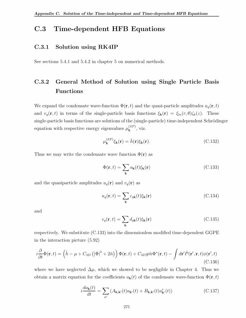
Appendix C. Solution of the Time-independent and Time-dependent HFB Equations
C.3 Time-dependent HFB Equations
C.3.1 Solution using RK4IP
See sections 5.4.1 and 5.4.2 in chapter 5 on numerical methods.
C.3.2 General Method of Solution using Single Particle Basis
Functions
We expand the condensate wave-function Φ(r, t) and the quasi-particle amplitudes uq(r, t)
and vq(r, t) in terms of the single-particle basis functions ξk(r) = ξln(r, θ)ζk(z). These
single-particle basis functions are solutions of the (single-particle) time-independent Schrodinger
equation with respective energy eigenvalues µ(SP )k , viz.
µ(SP )k ξk(r) = h(r)ξk(r). (C.132)
Thus we may write the condensate wave function Φ(r) as
Φ(r, t) =∑
k
ak(t)ξk(r) (C.133)
and the quasiparticle amplitudes uq(r) and vq(r) as
uq(r, t) =∑
k
cqk(t)ξk(r) (C.134)
and
vq(r, t) =∑
k
dqk(t)ξk(r) (C.135)
respectively. We substitute (C.133) into the dimensionless modified time-dependent GGPE
in the interaction picture (5.92)
i∂
∂tΦ(r, t) =
(
h− µ+ C3D
(
|Φ|2 + 2n)
)
Φ(r, t) + C3DgmΦ∗(r, t)−∫
dr′P (r′, r, t)φ(r′, t)
(C.136)
where we have neglected ∆µ, which we showed to be negligible in Chapter 4. Thus we
obtain a matrix equation for the coefficients ak(t) of the condensate wave-function Φ(r, t)
idak(t)
dt=∑
n′
(Ak,k′(t)ak′(t) +Bk,k′(t)a∗k′(t)) (C.137)
275
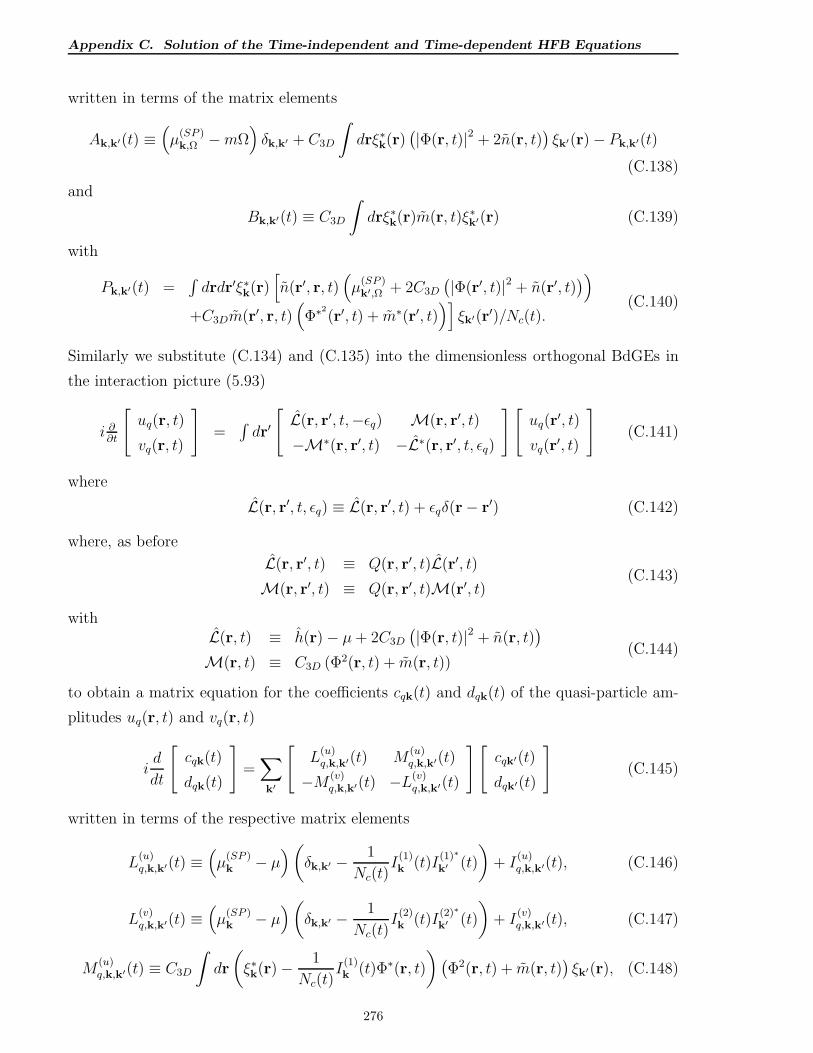
Appendix C. Solution of the Time-independent and Time-dependent HFB Equations
written in terms of the matrix elements
Ak,k′(t) ≡(
µ(SP )k,Ω −mΩ
)
δk,k′ + C3D
∫
drξ∗k(r)(
|Φ(r, t)|2 + 2n(r, t))
ξk′(r)− Pk,k′(t)
(C.138)
and
Bk,k′(t) ≡ C3D
∫
drξ∗k(r)m(r, t)ξ∗k′(r) (C.139)
with
Pk,k′(t) =∫
drdr′ξ∗k(r)[
n(r′, r, t)(
µ(SP )k′,Ω + 2C3D
(
|Φ(r′, t)|2 + n(r′, t))
)
+C3Dm(r′, r, t)(
Φ∗2(r′, t) + m∗(r′, t)
)]
ξk′(r′)/Nc(t).(C.140)
Similarly we substitute (C.134) and (C.135) into the dimensionless orthogonal BdGEs in
the interaction picture (5.93)
i ∂∂t
[
uq(r, t)
vq(r, t)
]
=∫
dr′
[
L(r, r′, t,−ǫq) M(r, r′, t)
−M∗(r, r′, t) −L∗(r, r′, t, ǫq)
][
uq(r′, t)
vq(r′, t)
]
(C.141)
where
L(r, r′, t, ǫq) ≡ L(r, r′, t) + ǫqδ(r− r′) (C.142)
where, as before
L(r, r′, t) ≡ Q(r, r′, t)L(r′, t)
M(r, r′, t) ≡ Q(r, r′, t)M(r′, t)(C.143)
withL(r, t) ≡ h(r)− µ+ 2C3D
(
|Φ(r, t)|2 + n(r, t))
M(r, t) ≡ C3D (Φ2(r, t) + m(r, t))(C.144)
to obtain a matrix equation for the coefficients cqk(t) and dqk(t) of the quasi-particle am-
plitudes uq(r, t) and vq(r, t)
id
dt
[
cqk(t)
dqk(t)
]
=∑
k′
[
L(u)q,k,k′(t) M
(u)q,k,k′(t)
−M (v)q,k,k′(t) −L(v)
q,k,k′(t)
][
cqk′(t)
dqk′(t)
]
(C.145)
written in terms of the respective matrix elements
L(u)q,k,k′(t) ≡
(
µ(SP )k − µ
)
(
δk,k′ − 1
Nc(t)I
(1)k (t)I
(1)∗
k′ (t)
)
+ I(u)q,k,k′(t), (C.146)
L(v)q,k,k′(t) ≡
(
µ(SP )k − µ
)
(
δk,k′ − 1
Nc(t)I
(2)k (t)I
(2)∗
k′ (t)
)
+ I(v)q,k,k′(t), (C.147)
M(u)q,k,k′(t) ≡ C3D
∫
dr
(
ξ∗k(r)−1
Nc(t)I
(1)k (t)Φ∗(r, t)
)
(
Φ2(r, t) + m(r, t))
ξk′(r), (C.148)
276
Appendix C. Solution of the Time-independent and Time-dependent HFB Equations
and
M(v)q,k,k′(t) ≡ C3D
∫
dr
(
ξ∗k(r)−1
Nc(t)I
(2)k (t)Φ(r, t)
)
(
Φ∗2
(r, t) + m∗(r, t))
ξk′(r), (C.149)
where
I(u)q,k,k′(t) ≡ C3D
∫
dr
(
ξ∗k(r)−1
Nc(t)I
(1)k (t)Φ∗(r, t)
)
(
|Φ(r, t)|2 + n(r, t))
ξk′(r), (C.150)
I(v)q,k,k′(t) ≡ C3D
∫
dr
(
ξ∗k(r)−1
Nc(t)I
(2)k (t)Φ(r, t)
)
(
|Φ(r, t)|2 + n(r, t))
ξk′(r), (C.151)
I(1)k (t) ≡
∫
drξ∗k(r)Φ(r, t), (C.152)
and
I(2)k (t) ≡
∫
drξ∗k(r)Φ∗(r, t). (C.153)
Defining the vectors a, cq and dq corresponding to the coefficients ak, cq,k and dq,k, and
the matrices A, B, L(u)q , M
(u)q , L
(v)q and M
(v)q corresponding to the matrix elements Ak,k′,
Bk,k′, L(u)q,k,k′, M
(u)q,k,k′, L
(v)q,k,k′ and M
(v)q,k,k′, we obtain the vector equation for the evolution of
the coefficients for the condensate wavefunction (GGPE)
ida(t)
dt= Aa(t) + Ba∗(t) (C.154)
which we can re-write in the form
id
dt
[
a(t)
a∗(t)
]
=
[
A B
−B∗ −A∗
][
a(t)
a∗(t)
]
, (C.155)
and for the quasiparticle amplitudes (BdGEs)
id
dt
[
cq(t)
dq(t)
]
=
[
L(u)q M
(u)q
−M(v)q −L
(v)q
][
cq(t)
dq(t)
]
. (C.156)
Each of these equations can be re-written in the form
dχ(t)
dt= f (χ(t), t) (C.157)
where
f (χ(t), t) ≡ Fχ(t). (C.158)
We can integrate the vector equation (C.157) using the standard fourth-order Runge-Kutta
algorithm, thus
f (χ(tn+1), tn+1) = f (χ(tn), tn) + [k1 + 2 (k2 + k3) + k4] /6 (C.159)
277
Appendix C. Solution of the Time-independent and Time-dependent HFB Equations
where
k1 = f (χ(tn), tn) ∆t, (C.160)
k2 = f
(
χ(tn +∆t
2) +
k1
2, tn +
∆t
2
)
∆t, (C.161)
k3 = f
(
χ(tn +∆t
2) +
k2
2, tn +
∆t
2
)
∆t, (C.162)
and
k4 = f (χ(tn + ∆t) + k3, tn + ∆t) ∆t. (C.163)
C.3.3 Solution of General 2D Case using Single Particle Basis
Functions
Let us consider the quasi-2D case (pancake BEC). We expand the condensate wave-
function Φ(r, θ, t) and quasiparticle amplitudes uq(r, θ, t), vq(r, θ, t) in the Laguerre basis
ξln(r, θ), l = 0,±1, . . . , n = 0, 1, . . .
(see (C.26), (C.27))
Φ(r, θ, t) =∑
ln
a0,ln(t)ξln(r, θ) (C.164)
uq(r, θ, t) =∑
ln
cq,ln(t)ξln(r, θ) (C.165)
and
vq(r, θ, t) =∑
ln
dq,ln(t)ξln(r, θ) (C.166)
where
ξln(r, θ) = ξln(r)eilθ
√2π. (C.167)
Substituting (C.164) into the GGPE (5.92), and (C.165), (C.166) into the orthogonal
BdGEs (5.93) in the interaction picture, we find that
idaln(t)
dt=∑
l′n′
(Aln,l′n′al′n′(t) +Bln,l′n′a∗l′n′(t)) (C.168)
and
id
dt
[
cq,ln(t)
dq,ln(t)
]
=∑
l′n′
[
L(u)q,ln,l′n′ M
(u)q,ln,l′n′
−M (v)q,ln,l′n′ −L(v)
q,ln,l′n′
][
cq,l′n′(t)
dq,l′n′(t)
]
(C.169)
where we have defined
Aln,l′n′(t) ≡ A′ln,l′n′(t)− Pln,l′n′(t), (C.170)
278
Appendix C. Solution of the Time-independent and Time-dependent HFB Equations
A′ln,l′n′(t) ≡
(
µ(SP )ln − lΩ− µ
)
δl,l′δn,n′+C2D
∞∫
0
2π∫
0
rdrdθξ∗ln(r, θ)(
|Φ(r, θ, t)|2 + 2n(r, θ, t))
ξl′n′(r, θ),
(C.171)
Pln,l′n′(t) ≡∫∞0
∫ 2π
0
∫∞0
∫ 2π
0rdrdθr′dr′dθ′ξ∗ln(r, θ) [
n(r′, θ′, r, θ, t)(
µ(SP )l′n′ − l′Ω− µ+ 2C2D
(
|Φ(r′, θ′, t)|2 + n(r′, θ′, t))
)
+C2Dm(r′, θ′, r, θ, t)(
Φ∗2(r′, θ′, t) + m∗(r′, θ′, t)
)]
ξl′n′(r′, θ′, t)/Nc(t),
(C.172)
Bln,l′n′(t) ≡ C2D
∞∫
0
2π∫
0
rdrdθξ∗ln(r, θ)m(r, θ, t)ξ∗l′n′(r, θ), (C.173)
L(u)q,ln,l′n′(t) ≡
(
µ(SP )ln − lΩ− µ− ǫq
)
(
δl,l′δn,n′ − 1
NcI
(1)ln (t)I
(1)∗
l′n′ (t)
)
+ I(u)q,ln,l′n′(t), (C.174)
L(v)q,ln,l′n′(t) ≡
(
µ(SP )ln + lΩ− µ+ ǫq
)
(
δl,l′δn,n′ − 1
NcI
(2)ln (t)I
(2)∗
l′n′ (t)
)
+ I(v)q,ln,l′n′(t), (C.175)
M(u)q,ln,l′n′(t) ≡ C2D
∞∫
0
2π∫
0
rdrdθ
(
ξ∗ln(r, θ)− 1
Nc
I(1)ln (t)Φ∗(r, θ, t)
)
(
Φ2(r, θ, t) + m(r, θ, t))
ξl′n′(r, θ),
(C.176)
and
M(v)q,ln,l′n′(t) ≡ C2D
∞∫
0
2π∫
0
rdrdθ
(
ξ∗ln(r, θ)− 1
NcI
(2)ln (t)Φ(r, θ, t)
)
(
Φ∗2
(r, θ, t) + m∗(r, θ, t))
ξl′n′(r, θ),
(C.177)
where
I(u)q,ln,l′n′(t) ≡ 2C2D
∞∫
0
2π∫
0
rdrdθ
(
ξ∗ln(r, θ)−1
NcI
(1)ln (t)Φ∗(r, θ, t)
)
(
|Φ(r, θ, t)|2 + n(r, θ, t))
ξl′n′(r, θ),
(C.178)
I(v)q,ln,l′n′(t) ≡ 2C2D
∞∫
0
2π∫
0
rdrdθ
(
ξ∗ln(r, θ)−1
NcI
(2)ln (t)Φ(r, θ, t)
)
(
|Φ(r, θ, t)|2 + n(r, θ, t))
ξl′n′(r, θ),
(C.179)
I(1)ln (t) ≡
∞∫
0
2π∫
0
rdrdθξ∗ln(r, θ)Φ(r, θ, t), (C.180)
and
I(2)ln (t) ≡
∞∫
0
2π∫
0
rdrdθξ∗ln(r, θ)Φ∗(r, θ, t). (C.181)
Defining the vectors a(t), cq(t) and dq(t) corresponding to the coefficients aln(t), cq,ln(t)
and dq,ln(t), and the matrices A, B, L(u)q , M
(u)q , L
(v)q and M
(v)q corresponding to the matrix
279
Appendix C. Solution of the Time-independent and Time-dependent HFB Equations
elements Aln,l′n′ , Bln,l′n′ , L(u)q,l,n,l′,n′, M
(u)q,l,n,l′,n′, L
(v)q,l,n,l′,n′ and M
(v)q,l,n,l′,n′, we obtain the vector
equation for the evolution of the coefficients for the condensate wavefunction (GGPE)
ida(t)
dt= Aa(t) + Ba∗(t) (C.182)
which we can re-write in the form
id
dt
[
a(t)
a∗(t)
]
=
[
A B
−B∗ −A∗
][
a(t)
a∗(t)
]
(C.183)
and for the quasiparticle amplitudes (BdGEs)
id
dt
[
cq(t)
dq(t)
]
=
[
L(u)q M
(u)q
−M(v)q −L
(v)q
][
cq(t)
dq(t)
]
. (C.184)
Each of these equations can be re-written in the form
dχ(t)
dt= f (χ(t), t) (C.185)
where
f (χ(t), t) ≡ Fχ(t) (C.186)
and we use the standard fourth-order Runge-Kutta algorithm as outlined in section C.3.2
above.
280
Appendix D. Perturbation Calculations for HFB
Appendix D
Perturbation Calculations for HFB
D.1 Calculation of Energy Shifts for Second Order
Perturbation as per Morgan [23,24]
D.1.1 Numerical Calculation
General Case
We calculate the energy shifts ∆ǫq using second-order perturbation theory according to S.
A. Morgan [23, 24], given by equation (2.151), thus
∆ǫq =∑
i,j 6=0
[
−∣
∣AP3qij
∣
∣
2(1 + ni + nj)
2(ǫq + ǫi + ǫj)+|Bqij + Bqji|2 (1 + ni + nj)
2(ǫq − ǫi − ǫj)+|Bijq +Biqj |2 (nj − ni)
ǫq − ǫi + ǫj)
]
(D.1)
where AP3ijk ≡ Aijk + Aikj + Ajik + Ajki + Akij + Akji , with Aijk and Bijk given by (2.147)
and (2.148). In the position representation, using the contact potential approximation,
Aijk and Bijk are given by (4.134)
Aijk = g
∫
dr (Φ∗viujuk + Φuivjvk) (D.2)
and (4.135)
Bijk = g
∫
dr (Φ∗ (u∗iujuk + v∗i vjuk + v∗i ujvk) + Φ (u∗iujvk + u∗i vjuk + v∗i vjvk)) (D.3)
We find that
Aqjk = Aqkj = g
∫
dr (Φ∗vqujuk + Φuqvjvk) ,
281
Appendix D. Perturbation Calculations for HFB
Ajqk = Ajkq = g
∫
dr (Φ∗uqvjuk + Φvqujvk)
and
Akqj = Akjq = g
∫
dr (Φ∗uqvkuj + Φvqukvj)
and therefore AP3qjk can be written
AP3qjk = 2g
∫
dr [(Φ∗uj + Φvj) (vquk + uqvk) + Φ∗vjuquk + Φujvqvk] (D.4)
From (D.3) we find that
Bqjk = Bqkj = g
∫
dr(
Φ∗ (u∗qujuk + v∗qvjuk + v∗qujvk
)
+ Φ(
u∗qujvk + u∗qvjuk + v∗qvjvk
))
and
Bjkq = Bjqk = g
∫
dr(
Φ∗ (uqu∗juk + uqv
∗j vk + vqv
∗juk
)
+ Φ(
vqu∗juk + uqu
∗jvk + vqv
∗j vk
))
and hence that
Bqjk +Bqkj = 2g
∫
dr[
(Φ∗uj + Φvj)(
u∗quk + v∗qvk
)
+ Φ∗vjv∗quk + Φuju
∗qvk
]
(D.5)
and
Bjkq +Bjqk = 2g
∫
dr[(
Φ∗v∗j + Φu∗j)
(uqvk + vquk) + Φ∗u∗juquk + Φv∗j vqvk
]
(D.6)
Let us define the functions
f(1)j (r) ≡ Φ(r)uj(r)
f(2)j (r) ≡ Φ∗(r)uj(r) + Φ(r)vj(r)
f(3)j (r) ≡ Φ∗(r)vj(r)
g(1)qk (r) ≡ uq(r)uk(r)
g(2)qk (r) ≡ uq(r)vk(r) + vq(r)uk(r)
g(3)qk (r) ≡ vq(r)vk(r)
h(1)qk (r) ≡ u∗q(r)vk(r)
h(2)qk (r) ≡ u∗q(r)uk(r) + v∗q (r)vk(r)
h(3)qk (r) ≡ v∗q (r)uk(r)
(D.7)
Then
AP3qjk = 2g
∫
dr[
f(1)j (r)g
(3)qk (r) + f
(2)j (r)g
(2)qk (r) + f
(3)j (r)g
(1)qk (r)
]
, (D.8)
Bqjk +Bqkj = 2g
∫
dr[
f(1)j (r)h
(1)qk (r) + f
(2)j (r)h
(2)qk (r) + f
(3)j (r)h
(3)qk (r)
]
, (D.9)
and
Bjkq +Bjqk = 2g
∫
dr[
f(1)∗
j (r)g(1)qk (r) + f
(2)∗
j (r)g(2)qk (r) + f
(3)∗
j (r)g(3)qk (r)
]
. (D.10)
282
Appendix D. Perturbation Calculations for HFB
Case of Axial Symmetry in 2D BEC
As before we integrate out the axial coordinate z, assuming the axial confinement to be
sufficiently strong that the higher axial energy modes can be ignored.
No Vortices Present Since no vortices are present, we can write
Φ(r, θ) = Φ(r)/√
2π
uln(r, θ) = uln(r) exp(ilθ)/√
2π
vln(r, θ) = vln(r) exp(ilθ)/√
2π
(D.11)
Thenf
(1)l′j (r, θ) = f
(1)l′j (r) exp(il′θ)/
√2π
f(2)l′j (r, θ) = f
(2)l′j (r) exp(il′θ)/
√2π
f(3)l′j (r, θ) = f
(3)l′j (r) exp(il′θ)/
√2π
g(1)lq,l′′k(r, θ) = g
(1)lq,l′′k(r) exp(i(l + l′′)θ)/
√2π
g(2)lq,l′′k(r, θ) = g
(2)lq,l′′k(r) exp(i(l + l′′)θ)/
√2π
g(3)lq,l′′k(r, θ) = g
(3)lq,l′′k(r) exp(i(l + l′′)θ)/
√2π
h(1)lq,l′′k(r, θ) = h
(1)lq,l′′k(r) exp(i(−l + l′′)θ)/
√2π
h(2)lq,l′′k(r, θ) = h
(2)lq,l′′k(r) exp(i(−l + l′′)θ)/
√2π
h(3)lq,l′′k(r, θ) = h
(3)lq,l′′k(r) exp(i(−l + l′′)θ)/
√2π
(D.12)
wheref
(1)l′j (r) = Φ(r)ul′j(r)
f(2)l′j (r) = Φ(r)ul′j(r) + Φ(r)vl′j(r)
f(3)l′j (r) = Φ(r)vl′j(r)
g(1)lq,l′′k(r) = ulq(r)ul′′k(r)
g(2)lq,l′′k(r) = ulq(r)vl′′k(r) + vlq(r)ul′′k(r)
g(3)lq,l′′k(r) = vlq(r)vl′′k(r)
h(1)lq,l′′k(r) = ulq(r)vl′′k(r)
h(2)lq,l′′k(r) = ulq(r)ul′′k(r) + vlq(r)vl′′k(r)
h(3)lq,l′′k(r) = vlq(r)ul′′k(r)
(D.13)
So in the dimensionless units used here
APlq,l′j,l′′k = 2NCR
2D
∫ ∞
0
rdr[
f(1)l′j g
(3)lq,l′′k + f
(2)l′j g
(2)lq,l′′k + f
(3)l′j g
(1)lq,l′′k
]
δl′′,−(l+l′), (D.14)
Blq,l′j,l′′k +Blq,l′′k,l′j = 2NCR2D
∫ ∞
0
rdr[
f(1)l′j h
(1)lq,l′′k + f
(2)l′j h
(2)lq,l′′k + f
(3)l′j h
(3)lq,l′′k
]
δl′′,l−l′, (D.15)
and
Blq,l′j,l′′k +Blq,l′′k,l′j = 2NCR2D
∫ ∞
0
rdr[
f(1)l′j g
(1)lq,l′′k + f
(2)l′j g
(2)lq,l′′k + f
(3)l′j g
(3)lq,l′′k
]
δl′′,l+l′. (D.16)
283
Appendix D. Perturbation Calculations for HFB
Single on-axis Vortex For a single on-axis vortex of charge m, we can write
Φ(r, θ) = Φ(r)/ exp(imθ)√
2π
uln(r, θ) = uln(r) exp(i(l +m)θ)/√
2π.
vln(r, θ) = vln(r) exp(i(l −m)θ)/√
2π
(D.17)
Then
f(1)l′j (r, θ) = f
(1)l′j (r) exp(i(l′ + 2m)θ)/
√2π
f(2)l′j (r, θ) = f
(2)l′j (r) exp(il′θ)/
√2π
f(3)l′j (r, θ) = f
(3)l′j (r) exp(i(l′ − 2m)θ)/
√2π
g(1)lq,l′′k(r, θ) = g
(1)lq,l′′k(r) exp(i(l + l′′ + 2m)θ)/
√2π
g(2)lq,l′′k(r, θ) = g
(2)lq,l′′k(r) exp(i(l + l′′)θ)/
√2π
g(3)lq,l′′k(r, θ) = g
(3)lq,l′′k(r) exp(i(l + l′′ − 2m)θ)/
√2π
h(1)lq,l′′k(r, θ) = h
(1)lq,l′′k(r) exp(i(−l + l′′ − 2m)θ)/
√2π
h(2)lq,l′′k(r, θ) = h
(2)lq,l′′k(r) exp(i(−l + l′′)θ)/
√2π
h(3)lq,l′′k(r, θ) = h
(3)lq,l′′k(r) exp(i(−l + l′′ + 2m)θ)/
√2π
(D.18)
where
f(1)l′j (r) = Φ(r)ul′j(r)
f(2)l′j (r) = Φ(r)ul′j(r) + Φ(r)vl′j(r)
f(3)l′j (r) = Φ(r)vl′j(r)
g(1)lq,l′′k(r) = ulq(r)ul′′k(r)
g(2)lq,l′′k(r) = ulq(r)vl′′k(r) + vlq(r)ul′′k(r)
g(3)lq,l′′k(r) = vlq(r)vl′′k(r)
h(1)lq,l′′k(r) = ulq(r)vl′′k(r)
h(2)lq,l′′k(r) = ulq(r)ul′′k(r) + vlq(r)vl′′k(r)
h(3)lq,l′′k(r) = vlq(r)ul′′k(r)
(D.19)
So in the dimensionless units used here
APlq,l′j,l′′k = 2NCR
2D
∫ ∞
0
rdr[
f(1)l′j g
(3)lq,l′′k + f
(2)l′j g
(2)lq,l′′k + f
(3)l′j g
(1)lq,l′′k
]
δl′′,−(l+l′), (D.20)
Blq,l′j,l′′k +Blq,l′′k,l′j = 2NCR2D
∫ ∞
0
rdr[
f(1)l′j h
(1)lq,l′′k + f
(2)l′j h
(2)lq,l′′k + f
(3)l′j h
(3)lq,l′′k
]
δl′′,l−l′, (D.21)
and
Blq,l′j,l′′k +Blq,l′′k,l′j = 2NCR2D
∫ ∞
0
rdr[
f(1)l′j g
(1)lq,l′′k + f
(2)l′j g
(2)lq,l′′k + f
(3)l′j g
(3)lq,l′′k
]
δl′′,l+l′ (D.22)
as in the case of no vortices.
284
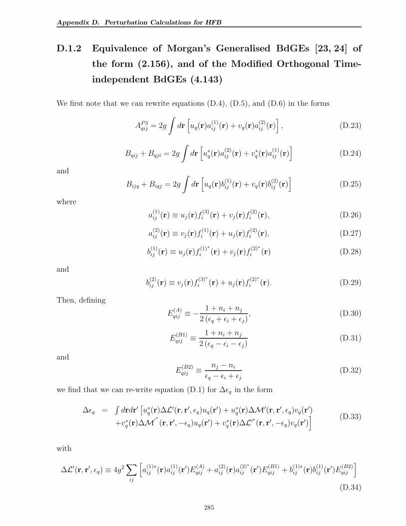
Appendix D. Perturbation Calculations for HFB
D.1.2 Equivalence of Morgan’s Generalised BdGEs [23, 24] of
the form (2.156), and of the Modified Orthogonal Time-
independent BdGEs (4.143)
We first note that we can rewrite equations (D.4), (D.5), and (D.6) in the forms
AP3qij = 2g
∫
dr[
uq(r)a(1)ij (r) + vq(r)a
(2)ij (r)
]
, (D.23)
Bqij +Bqji = 2g
∫
dr[
u∗q(r)a(2)ij (r) + v∗q (r)a
(1)ij (r)
]
(D.24)
and
Bijq +Biqj = 2g
∫
dr[
uq(r)b(1)ij (r) + vq(r)b
(2)ij (r)
]
(D.25)
where
a(1)ij (r) ≡ uj(r)f
(3)i (r) + vj(r)f
(2)i (r), (D.26)
a(2)ij (r) ≡ vj(r)f
(1)i (r) + uj(r)f
(2)i (r), (D.27)
b(1)ij (r) ≡ uj(r)f
(1)∗
i (r) + vj(r)f(2)∗
i (r) (D.28)
and
b(2)ij (r) ≡ vj(r)f
(3)∗
i (r) + uj(r)f(2)∗
i (r). (D.29)
Then, defining
E(A)qij ≡ −
1 + ni + nj
2 (ǫq + ǫi + ǫj), (D.30)
E(B1)qij ≡
1 + ni + nj
2 (ǫq − ǫi − ǫj)(D.31)
and
E(B2)qij ≡
nj − ni
ǫq − ǫi + ǫj(D.32)
we find that we can re-write equation (D.1) for ∆ǫq in the form
∆ǫq =∫
drdr′[
u∗q(r)∆L′(r, r′, ǫq)uq(r′) + u∗q(r)∆M′(r, r′, ǫq)vq(r
′)
+v∗q (r)∆M′∗
(r, r′,−ǫq)uq(r′) + v∗q (r)∆L′∗(r, r′,−ǫq)vq(r
′)] (D.33)
with
∆L′(r, r′, ǫq) ≡ 4g2∑
ij
[
a(1)∗ij (r)a
(1)ij (r′)E
(A)qij + a
(2)ij (r)a
(2)∗
ij (r′)E(B1)qij + b
(1)∗ij (r)b
(1)ij (r′)E
(B2)qij
]
(D.34)
285
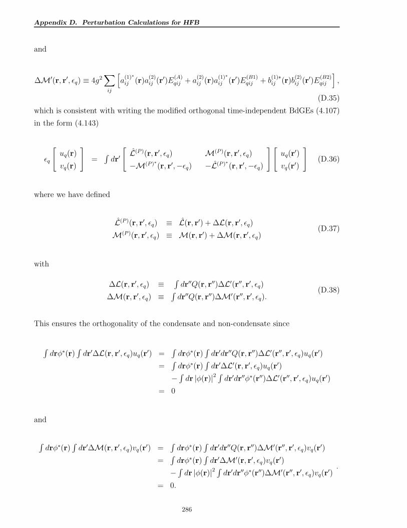
Appendix D. Perturbation Calculations for HFB
and
∆M′(r, r′, ǫq) ≡ 4g2∑
ij
[
a(1)∗
ij (r)a(2)ij (r′)E
(A)qij + a
(2)ij (r)a
(1)∗
ij (r′)E(B1)qij + b
(1)∗ij (r)b
(2)ij (r′)E
(B2)qij
]
,
(D.35)
which is consistent with writing the modified orthogonal time-independent BdGEs (4.107)
in the form (4.143)
ǫq
[
uq(r)
vq(r)
]
=∫
dr′
[
L(P )(r, r′, ǫq) M(P )(r, r′, ǫq)
−M(P )∗(r, r′,−ǫq) −L(P )∗(r, r′,−ǫq)
][
uq(r′)
vq(r′)
]
(D.36)
where we have defined
L(P )(r, r′, ǫq) ≡ L(r, r′) + ∆L(r, r′, ǫq)
M(P )(r, r′, ǫq) ≡ M(r, r′) + ∆M(r, r′, ǫq)(D.37)
with
∆L(r, r′, ǫq) ≡∫
dr′′Q(r, r′′)∆L′(r′′, r′, ǫq)
∆M(r, r′, ǫq) ≡∫
dr′′Q(r, r′′)∆M′(r′′, r′, ǫq).(D.38)
This ensures the orthogonality of the condensate and non-condensate since
∫
drφ∗(r)∫
dr′∆L(r, r′, ǫq)uq(r′) =
∫
drφ∗(r)∫
dr′dr′′Q(r, r′′)∆L′(r′′, r′, ǫq)uq(r′)
=∫
drφ∗(r)∫
dr′∆L′(r, r′, ǫq)uq(r′)
−∫
dr |φ(r)|2∫
dr′dr′′φ∗(r′′)∆L′(r′′, r′, ǫq)uq(r′)
= 0
and
∫
drφ∗(r)∫
dr′∆M(r, r′, ǫq)vq(r′) =
∫
drφ∗(r)∫
dr′dr′′Q(r, r′′)∆M′(r′′, r′, ǫq)vq(r′)
=∫
drφ∗(r)∫
dr′∆M′(r, r′, ǫq)vq(r′)
−∫
dr |φ(r)|2∫
dr′dr′′φ∗(r′′)∆M′(r′′, r′, ǫq)vq(r′)
= 0.
.
286
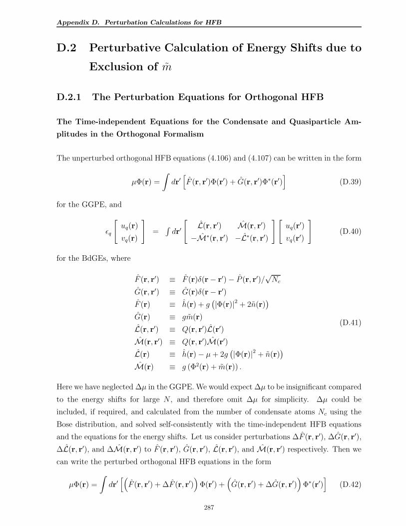
Appendix D. Perturbation Calculations for HFB
D.2 Perturbative Calculation of Energy Shifts due to
Exclusion of m
D.2.1 The Perturbation Equations for Orthogonal HFB
The Time-independent Equations for the Condensate and Quasiparticle Am-
plitudes in the Orthogonal Formalism
The unperturbed orthogonal HFB equations (4.106) and (4.107) can be written in the form
µΦ(r) =
∫
dr′[
F (r, r′)Φ(r′) + G(r, r′)Φ∗(r′)]
(D.39)
for the GGPE, and
ǫq
[
uq(r)
vq(r)
]
=∫
dr′
[
L(r, r′) M(r, r′)
−M∗(r, r′) −L∗(r, r′)
][
uq(r′)
vq(r′)
]
(D.40)
for the BdGEs, where
F (r, r′) ≡ F (r)δ(r− r′)− P (r, r′)/√Nc
G(r, r′) ≡ G(r)δ(r− r′)
F (r) ≡ h(r) + g(
|Φ(r)|2 + 2n(r))
G(r) ≡ gm(r)
L(r, r′) ≡ Q(r, r′)L(r′)
M(r, r′) ≡ Q(r, r′)M(r′)
L(r) ≡ h(r)− µ+ 2g(
|Φ(r)|2 + n(r))
M(r) ≡ g (Φ2(r) + m(r)) .
(D.41)
Here we have neglected ∆µ in the GGPE. We would expect ∆µ to be insignificant compared
to the energy shifts for large N , and therefore omit ∆µ for simplicity. ∆µ could be
included, if required, and calculated from the number of condensate atoms Nc using the
Bose distribution, and solved self-consistently with the time-independent HFB equations
and the equations for the energy shifts. Let us consider perturbations ∆F (r, r′), ∆G(r, r′),
∆L(r, r′), and ∆M(r, r′) to F (r, r′), G(r, r′), L(r, r′), and M(r, r′) respectively. Then we
can write the perturbed orthogonal HFB equations in the form
µΦ(r) =
∫
dr′[(
F (r, r′) + ∆F (r, r′))
Φ(r′) +(
G(r, r′) + ∆G(r, r′))
Φ∗(r′)]
(D.42)
287
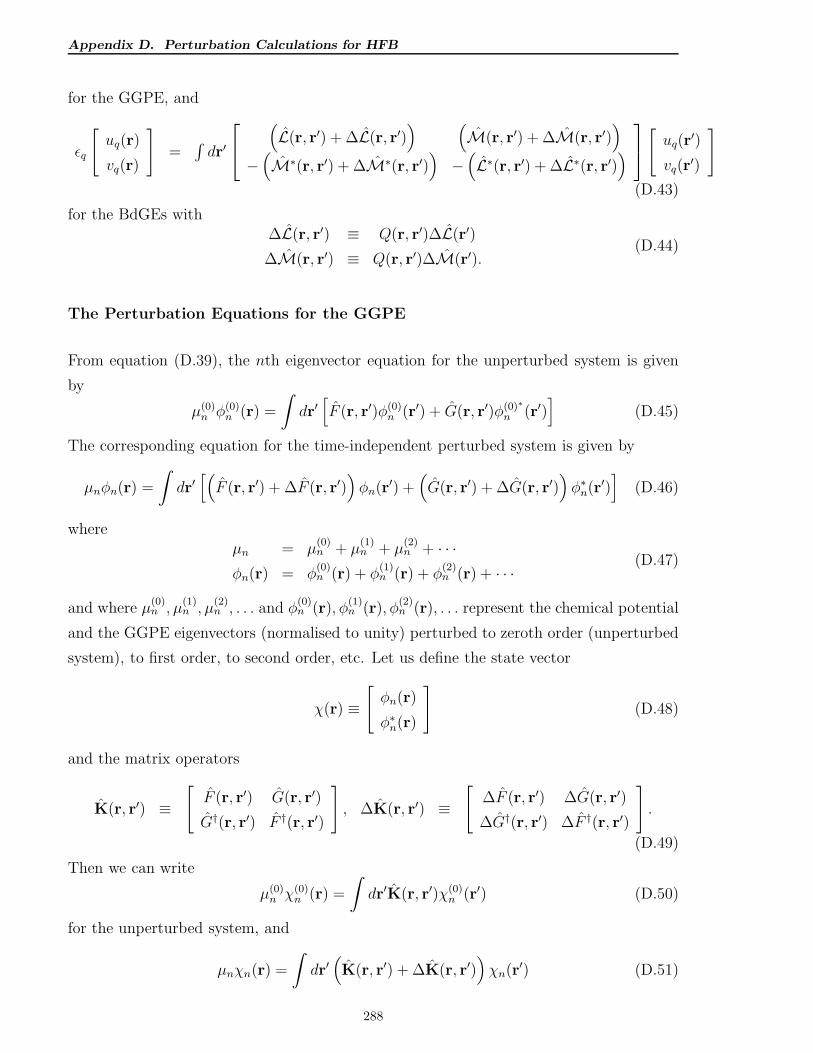
Appendix D. Perturbation Calculations for HFB
for the GGPE, and
ǫq
[
uq(r)
vq(r)
]
=∫
dr′
(
L(r, r′) + ∆L(r, r′)) (
M(r, r′) + ∆M(r, r′))
−(
M∗(r, r′) + ∆M∗(r, r′))
−(
L∗(r, r′) + ∆L∗(r, r′))
[
uq(r′)
vq(r′)
]
(D.43)
for the BdGEs with∆L(r, r′) ≡ Q(r, r′)∆L(r′)
∆M(r, r′) ≡ Q(r, r′)∆M(r′).(D.44)
The Perturbation Equations for the GGPE
From equation (D.39), the nth eigenvector equation for the unperturbed system is given
by
µ(0)n φ(0)
n (r) =
∫
dr′[
F (r, r′)φ(0)n (r′) + G(r, r′)φ(0)∗
n (r′)]
(D.45)
The corresponding equation for the time-independent perturbed system is given by
µnφn(r) =
∫
dr′[(
F (r, r′) + ∆F (r, r′))
φn(r′) +(
G(r, r′) + ∆G(r, r′))
φ∗n(r
′)]
(D.46)
whereµn = µ
(0)n + µ
(1)n + µ
(2)n + · · ·
φn(r) = φ(0)n (r) + φ
(1)n (r) + φ
(2)n (r) + · · ·
(D.47)
and where µ(0)n , µ
(1)n , µ
(2)n , . . . and φ
(0)n (r), φ
(1)n (r), φ
(2)n (r), . . . represent the chemical potential
and the GGPE eigenvectors (normalised to unity) perturbed to zeroth order (unperturbed
system), to first order, to second order, etc. Let us define the state vector
χ(r) ≡[
φn(r)
φ∗n(r)
]
(D.48)
and the matrix operators
K(r, r′) ≡[
F (r, r′) G(r, r′)
G†(r, r′) F †(r, r′)
]
, ∆K(r, r′) ≡[
∆F (r, r′) ∆G(r, r′)
∆G†(r, r′) ∆F †(r, r′)
]
.
(D.49)
Then we can write
µ(0)n χ(0)
n (r) =
∫
dr′K(r, r′)χ(0)n (r′) (D.50)
for the unperturbed system, and
µnχn(r) =
∫
dr′(
K(r, r′) + ∆K(r, r′))
χn(r′) (D.51)
288
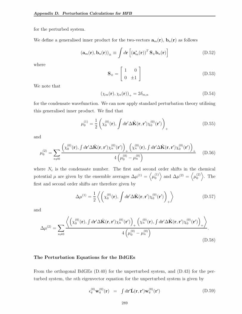
Appendix D. Perturbation Calculations for HFB
for the perturbed system.
We define a generalised inner product for the two-vectors am(r), bn(r) as follows
(am(r),bn(r))± ≡∫
dr[
(a∗m(r))T S±bn(r)
]
(D.52)
where
S± =
[
1 0
0 ±1
]
(D.53)
We note that
(χm(r), χn(r))+ = 2δm,n (D.54)
for the condensate wavefunction. We can now apply standard perturbation theory utilising
this generalised inner product. We find that
µ(1)0 =
1
2
(
χ(0)0 (r),
∫
dr′∆K(r, r′)χ(0)0 (r′)
)
+
(D.55)
and
µ(2)0 =
∑
n 6=0
(
χ(0)0 (r),
∫
dr′∆K(r, r′)χ(0)n (r′)
)
+
(
χ(0)n (r),
∫
dr′∆K(r, r′)χ(0)0 (r′)
)
+
4(
µ(0)0 − µ
(0)n
) (D.56)
where Nc is the condensate number. The first and second order shifts in the chemical
potential µ are given by the ensemble averages ∆µ(1) =⟨
µ(1)0
⟩
and ∆µ(2) =⟨
µ(2)0
⟩
. The
first and second order shifts are therefore given by
∆µ(1) =1
2
⟨(
χ(0)0 (r),
∫
dr′∆K(r, r′)χ(0)0 (r′)
)
+
⟩
(D.57)
and
∆µ(2) =∑
n 6=0
⟨
(
χ(0)0 (r),
∫
dr′∆K(r, r′)χ(0)n (r′)
)
+
(
χ(0)n (r),
∫
dr′∆K(r, r′)χ(0)0 (r′)
)
+
⟩
4(
µ(0)0 − µ
(0)n
) .
(D.58)
The Perturbation Equations for the BdGEs
From the orthogonal BdGEs (D.40) for the unperturbed system, and (D.43) for the per-
turbed system, the nth eigenvector equation for the unperturbed system is given by
ǫ(0)q w
(0)q (r) =
∫
dr′L(r, r′)w(0)q (r′) (D.59)
289
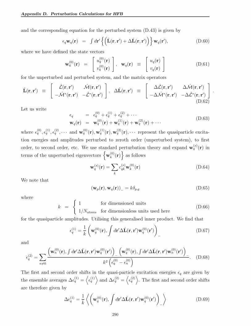
Appendix D. Perturbation Calculations for HFB
and the corresponding equation for the perturbed system (D.43) is given by
ǫqwq(r) =∫
dr′(
L(r, r′) + ∆L(r, r′))
wq(r′), (D.60)
where we have defined the state vectors
w(0)q (r) =
[
u(0)q (r)
v(0)q (r)
]
, wq(r) ≡[
uq(r)
vq(r)
]
(D.61)
for the unperturbed and perturbed system, and the matrix operators
L(r, r′) ≡[
L(r, r′) M(r, r′)
−M∗(r, r′) −L∗(r, r′)
]
, ∆L(r, r′) ≡[
∆L(r, r′) ∆M(r, r′)
−∆M∗(r, r′) −∆L∗(r, r′)
]
.
(D.62)
Let us writeǫq = ǫ
(0)q + ǫ
(1)q + ǫ
(2)q + · · ·
wq(r) = w(0)q (r) + w
(1)q (r) + w
(2)q (r) + · · ·
(D.63)
where ǫ(0)q , ǫ
(1)q , ǫ
(2)q , · · · and w
(0)q (r),w
(1)q (r),w
(2)q (r), · · · represent the quasiparticle excita-
tion energies and amplitudes perturbed to zeroth order (unperturbed system), to first
order, to second order, etc. We use standard perturbation theory and expand w(s)q (r) in
terms of the unperturbed eigenvectors
w(0)k (r)
as follows
w(s)q (r) =
∑
k
c(s)qk w
(0)k (r) (D.64)
We note that
(wp(r),wq(r))− = kδp,q (D.65)
where
k =
1 for dimensioned units
1/Natoms for dimensionless units used here(D.66)
for the quasiparticle amplitudes. Utilising this generalised inner product. We find that
ǫ(1)q =1
k
(
w(0)q (r),
∫
dr′∆L(r, r′)w(0)q (r′)
)
−(D.67)
and
ǫ(2)q =∑
n 6=0
(
w(0)n (r),
∫
dr′∆L(r, r′)w(0)q (r′)
)
−
(
w(0)q (r),
∫
dr′∆L(r, r′)w(0)n (r′)
)
−
k2(
ǫ(0)q − ǫ(0)n
) . (D.68)
The first and second order shifts in the quasi-particle excitation energies ǫq are given by
the ensemble averages ∆ǫ(1)q =
⟨
ǫ(1)q
⟩
and ∆ǫ(2)q =
⟨
ǫ(2)q
⟩
. The first and second order shifts
are therefore given by
∆ǫ(1)q =1
k
⟨(
w(0)q (r),
∫
dr′∆L(r, r′)w(0)q (r′)
)
−
⟩
(D.69)
290
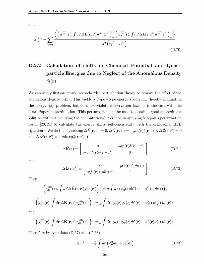
Appendix D. Perturbation Calculations for HFB
and
∆ǫ(2)q =∑
n 6=0
⟨
(
w(0)n (r),
∫
dr′∆L(r, r′)w(0)q (r′)
)
−
(
w(0)q (r),
∫
dr′∆L(r, r′)w(0)n (r′)
)
−
⟩
k2(
ǫ(0)q − ǫ(0)n
) .
(D.70)
D.2.2 Calculation of shifts in Chemical Potential and Quasi-
particle Energies due to Neglect of the Anomalous Density
m(r)
We can apply first-order and second-order perturbation theory to remove the effect of the
anomalous density m(r). This yields a Popov-type energy spectrum, thereby eliminating
the energy gap problem, but does not violate conservation laws as is the case with the
usual Popov approximation. This perturbation can be used to obtain a good approximate
solution without incurring the computational overhead in applying Morgan’s perturbation
result [23, 24] to calculate the energy shifts self-consistently with the orthogonal HFB
equations. We do this by setting ∆F (r, r′) = 0, ∆G(r, r′) = −gm(r)δ(r−r′), ∆L(r, r′) = 0
and ∆M(r, r′) = −gm(r)Q(r, r′), thus
∆K(r) ≡[
0 −gm(r)δ(r− r′)
−gm∗(r)δ(r− r′) 0
]
(D.71)
and
∆L(r, r′) ≡[
0 −gQ(r, r′)m(r′)
gQ∗(r, r′)m∗(r′) 0
]
(D.72)
Then(
χ(0)0 (r),
∫
dr′∆K(r, r′)χ(0)0 (r′)
)
+
= g
∫
dr(
φ20(r)m
∗(r) + φ∗2
0 (r)m(r))
,
(
χ(0)0 (r),
∫
dr′∆K(r, r′)χ(0)n (r′)
)
+
= g
∫
dr (φ0(r)φn(r)m∗(r) + φ∗0(r)φ
∗n(r)m(r)) ,
and(
χ(0)n (r),
∫
dr′∆K(r, r′)χ(0)0 (r′)
)
+
= g
∫
dr (φn(r)φ0(r)m∗(r) + φ∗
n(r)φ∗0(r)m(r)) .
Therefore by equations (D.57) and (D.58)
∆µ(1) = −g2
∫
dr(
φ20m
∗ + φ∗2
0 m)
(D.73)
291
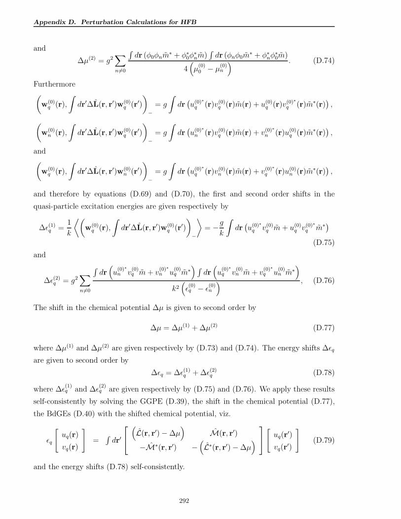
Appendix D. Perturbation Calculations for HFB
and
∆µ(2) = g2∑
n 6=0
∫
dr (φ0φnm∗ + φ∗
0φ∗nm)
∫
dr (φnφ0m∗ + φ∗
nφ∗0m)
4(
µ(0)0 − µ
(0)n
) . (D.74)
Furthermore(
w(0)q (r),
∫
dr′∆L(r, r′)w(0)q (r′)
)
−= g
∫
dr(
u(0)∗
q (r)v(0)q (r)m(r) + u(0)
q (r)v(0)∗
q (r)m∗(r))
,
(
w(0)n (r),
∫
dr′∆L(r, r′)w(0)q (r′)
)
−= g
∫
dr(
u(0)∗
n (r)v(0)q (r)m(r) + v(0)∗
n (r)u(0)q (r)m∗(r)
)
,
and(
w(0)q (r),
∫
dr′∆L(r, r′)w(0)n (r′)
)
−= g
∫
dr(
u(0)∗
q (r)v(0)n (r)m(r) + v(0)∗
q (r)u(0)n (r)m∗(r)
)
,
and therefore by equations (D.69) and (D.70), the first and second order shifts in the
quasi-particle excitation energies are given respectively by
∆ǫ(1)q =1
k
⟨(
w(0)q (r),
∫
dr′∆L(r, r′)w(0)q (r′)
)
−
⟩
= −gk
∫
dr(
u(0)∗
q v(0)q m+ u(0)
q v(0)∗
q m∗)
(D.75)
and
∆ǫ(2)q = g2∑
n 6=0
∫
dr(
u(0)∗
n v(0)q m+ v
(0)∗
n u(0)q m∗
)
∫
dr(
u(0)∗
q v(0)n m+ v
(0)∗
q u(0)n m∗
)
k2(
ǫ(0)q − ǫ(0)n
) , (D.76)
The shift in the chemical potential ∆µ is given to second order by
∆µ = ∆µ(1) + ∆µ(2) (D.77)
where ∆µ(1) and ∆µ(2) are given respectively by (D.73) and (D.74). The energy shifts ∆ǫq
are given to second order by
∆ǫq = ∆ǫ(1)q + ∆ǫ(2)q (D.78)
where ∆ǫ(1)q and ∆ǫ
(2)q are given respectively by (D.75) and (D.76). We apply these results
self-consistently by solving the GGPE (D.39), the shift in the chemical potential (D.77),
the BdGEs (D.40) with the shifted chemical potential, viz.
ǫq
[
uq(r)
vq(r)
]
=∫
dr′
(
L(r, r′)−∆µ)
M(r, r′)
−M∗(r, r′) −(
L∗(r, r′)−∆µ)
[
uq(r′)
vq(r′)
]
(D.79)
and the energy shifts (D.78) self-consistently.
292
Appendix E. Two-state and Multi-state Models for Vortices in BECs
Appendix E
Two-state and Multi-state Models for
Vortices in BECs
E.1 Two-state Model
Consider the two-state model presented in section 7.3.1 given by two-mode superposition
states of the form [90,105]
Φ(r, θ, t) =1√2π
(
ag(t)φg(r) + av(t)φv(r)eiθ)
(E.1)
whereag(t) = ag0e
−iµgt
av(t) = av0e−iµvt
(E.2)
We solve this by transforming to the rotating frame. In the rotating frame
h(r, θ)→ hΩ(r, θ) = h(r, θ) + iΩ∂
∂θ(E.3)
so
hl(r)→ hΩ,l(r) = hl(r)− Ωl (E.4)
In the co-rotating frame θ → θ − Ωt, a stationary solution can be found, and the ansatz
(E.1) becomes
Φ(r, θ, t) = e−iµtΦ(r, θ) = e−iµt 1√2π
(
ag0φg(r) + av0φv(r)eiθ)
(E.5)
Here the chemical potential is given by
µ = µg (E.6)
293
Appendix E. Two-state and Multi-state Models for Vortices in BECs
and the precessional frequency of the vortex by
Ω = µv − µg (E.7)
E.1.1 The Coupled GGPEs in the Rotating Frame
In the frame rotating at the precessional frequency Ω, we obtain the coupled GGPEs
µφg =[
hΩ,0 + CR′
2D
(
ng0 |φg|2 + 2nv0 |φv|2 + 2N (0) + M (0))]
φg+av0
ag0
CR′
2D
(
2N (1) + M (−1))
φv
(E.8)
and
µφv =[
hΩ,1 + CR′
2D
(
nv0 |φv|2 + 2ng0 |φg|2 + 2N (0) + M (−2))]
φv+ag0
av0
CR′
2D
(
2N (−1) + M (−1))
φg
(E.9)
whereng0 = |ag0|2
nv0 = |av0 |2 ,(E.10)
and where we have defined the quantities
N (l)c (r) ≡
∫ 2π
0
eilθ
√2πnc(r, θ)dθ, (E.11)
N (l)(r) ≡∫ 2π
0
eilθ
√2πn(r, θ)dθ, (E.12)
and
M (l)(r) ≡∫ 2π
0
eilθ
√2πm(r, θ)dθ. (E.13)
We show this as follows:
In the co-rotating frame
(
−∇2 + V)
Φ = e−iµt 1√2π
(
ag0hΩ,0φg + av0eiθhΩ,1φv
)
(E.14)
and
|Φ|2 =1
2π
(
|ag0|2 |φg|2 + ag0av0eiθφsφv + ag0av0e
−iθφsφv + |av0 |2 |φv|2)
(E.15)
so noting that CR2D = C2D/2π, we obtain
C2D
(
|Φ|2 + 2n)
Φ = e−iµtCR2D
[
|ag0 |2 |φg|2 ag0φg + 2 |av0 |2 |φv|2 ag0φg + 2nag0φg
]
+[
|av0 |2 |φv|2 av0φv + 2 |ag0|2 |φg|2 av0φv + 2nav0φv
]
exp(iθ)
+a2gav0φ
2gφv exp(−iθ) + ag0a
2vφgφ
2v exp(2iθ)
(E.16)
294
Appendix E. Two-state and Multi-state Models for Vortices in BECs
and
C2Dm(r, θ, t)Φ∗ = eiµtCR2Dm(r, θ, t)
(
ag0φg + av0φve−iθ)
= e−iµtCR2Dm(r, θ)
(
ag0φg + av0φve−iθ)
(E.17)
where we note that m(r, θ, t) has phase −2iµt in order to satisfy the stationary condition
for the GGPEs, ie.
m(r, θ, t) = e−2iµtm(r, θ) (E.18)
Now by (E.2) and (E.5)(
idag
dt
)
φg =1√2π
∫ 2π
0
i∂Φ
∂tdθ
and(
idav
dt
)
φg =1√2π
∫ 2π
0
e−iθi∂Φ
∂tdθ
and since now (cf (E.2), (E.6) and (E.7))
idag
dt= µag (E.19)
and
idav
dt= µav (E.20)
in the co-rotating frame, we obtain the coupled GGPEs
µφg =[
hΩ,0 + CR2D
(
ng0 |φg|2 + 2nv0 |φv|2 + 2N (0) + M (0))]
φg+av0
ag0
CR2D
(
2N (1) + M (−1))
φv
(E.21)
and
µφv =[
hΩ,1 + CR2D
(
nv0 |φv|2 + 2ng0 |φg|2 + 2N (0) + M (−2))]
φv+ag0
av0
CR2D
(
2N (−1) + M (−1))
φg.
(E.22)
Let us define the operators Fg,Ω, Gg, Fv,Ω, and Gv for the frame rotating about the axis of
symmetry at angular frequency Ω given respectively by
Fg,Ω ≡ hΩ,0 + CR′
2D
(
ng0 |φg|2 + 2nv0 |φv|2 + 2N (0) + M (0))
= Fg (E.23)
Gg ≡av0
ag0
CR′
2D
(
2N (1) + M (−1))
(E.24)
Fv,Ω ≡ hΩ,1 + CR′
2D
(
nv0 |φv|2 + 2ng0 |φg|2 + 2N (0) + M (−2))
= Fv − Ω (E.25)
and
Gv ≡ag0
av0
CR′
2D
(
2N (−1) + M (−1))
. (E.26)
Then the GGPEs in the rotating frame can be rewritten in the matrix form
µ
[
φg
φv
]
=
[
Fg,Ω Gg
Gv Fv,Ω
][
φg
φv
]
. (E.27)
295
Appendix E. Two-state and Multi-state Models for Vortices in BECs
E.1.2 The BdGEs
We first note that we can write
uq(r, θ, t) = e−iµtuq(r, θ) (E.28)
and
vq(r, θ, t) = eiµtvq(r, θ) (E.29)
so that (E.18) is satisfied.
We expand the quasi-particle amplitudes in terms of the complete single-particle basis
ξln(r)eilθ
√2π| n = 0, 1, . . . ; l = 0,±1, . . .
(E.30)
and write
uq(r, θ) =∑
nl
cq,lnξln(r)eilθ
√2π
=∑
l
u(l)q (r)
eilθ
√2π
(E.31)
and
vq(r, θ) =∑
nl
dq,lnξln(r)eilθ
√2π
=∑
l
v(l)q (r)
eilθ
√2π. (E.32)
The BdGE for uq in the co-rotating frame is given by
ǫquq =(
hΩ − µ+ 2CR2D
(
|Φ|2 + n)
)
uq + CR2D
(
Φ2 + m)
vq (E.33)
so
ǫq∑
l u(l)q (r) eilθ√
2π=∑
l
[
hΩ − µ+ 2CR2D
(
ng0 |φg|2 + ag0av0eiθφgφv + ag0av0e
−iθφsφv
+ |av0 |2 |φv|2 + n)]
u(l)q (r) eilθ
√2π
+ CR2D
[
a2g0φ2
g + 2ag0av0φgφveiθ + a2
v0φ2
ve2iθ + m
]
v(l)q (r) eilθ
√2π
.
(E.34)
Therefore, multiplying by e−ilθ/√
2π, and integrating over all θ, and defining the quantities
L(u)ll′ =
hΩ,l + 2CR′
2D
(
ng0 |φg|2 + nv0 |φv|2 + N (0))
, l′ = l
2CR′
2D
(
ag0av0φgφv + N (±1))
, l′ = l ± 1
2CR′
2DN(l′−l) , l′ /∈ l, l ± 1
(E.35)
and
M(u)ll′ =
CR′
2D
(
a2g0φ2
g + M (0))
, l′ = l
CR′
2D
(
2ag0av0φgφv + M (−1))
, l′ = l − 1
CR′
2D
(
a2v0φ2
v + M (−2))
, l′ = l − 2
CR′
2DM(l′−l) , l′ /∈ l, l − 1, l − 2
(E.36)
296
Appendix E. Two-state and Multi-state Models for Vortices in BECs
we find that
ǫqu(l)q =
∑
l′
(
L(u)ll′ u
(l′)q + M(u)
ll′ v(l′)q
)
. (E.37)
The BdGE for vq in the co-rotating frame is given by
−ǫqvq =(
h∗Ω − µ+ 2CR2D
(
|Φ|2 + n)
)
vq + CR2D
(
Φ∗2
+ m∗)
uq (E.38)
so
−ǫq∑
l v(l)q (r) eilθ
√2π
=∑
l
[
h∗Ω − µ+ 2CR2D
(
ng0 |φg|2 + ag0av0eiθφgφv + ag0av0e
−iθφsφv
+ |av0 |2 |φv|2 + n)]
v(l)q (r)(r) eilθ
√2π
+ CR2D
[
a2g0φ2
g + 2ag0av0φgφve−iθ + a2
v0φ2
ve2iθ + m∗]u
(l)q (r) eilθ
√2π
.
(E.39)
So again, multiplying by e−ilθ/√
2π, and integrating over all θ, and defining the quantities
L(v)ll′ =
hΩ,−l + 2CR′
2D
(
ng0 |φg|2 + nv0 |φv|2 + N (0))
, l′ = l
2CR′
2D
(
ag0av0φgφv + N (±1))
, l′ = l ± 1
2CR′
2DN(l′−l) , l′ /∈ l, l ± 1
(E.40)
and
M(v)ll′ =
CR′
2D
(
a2g0φ2
g + M (0))
, l′ = l
CR′
2D
(
2ag0av0φgφv + M (−1))
, l′ = l + 1
CR′
2D
(
a2v0φ2
v + M (−2))
, l′ = l + 2
CR′
2DM(l′−l) , l′ /∈ l, l + 1, l + 2
(E.41)
we find that
−ǫqv(l)q =
∑
l′
(
L(v)ll′ v
(l′)q + M(v)
ll′ u(l′)q
)
. (E.42)
Defining the vectors uq, and vq corresponding to the u(l)q (r) and the v
(l)q (r) and the matrix
operators Lu, Mu, Lv, and Mv corresponding to the L(u)ll′ , the M(u)
ll′ , the L(v)ll′ and the M(v)
ll′
respectively, we obtain the BdGEs
[
Lu Mu
−Mv −Lv
][
uq
vq
]
= ǫq
[
uq
vq
]
. (E.43)
We solve the two-state GGPE (E.27) and BdGEs (E.43) for various values of α lying
between 0 and 1 and for various values of ag and av in the zero temperature limit.
297
Appendix E. Two-state and Multi-state Models for Vortices in BECs
E.2 Generalised Multi-state Model
We generalise the two-state model [90,105], and write the following ansatz for the conden-
sate wave function
Φ(r, θ, t) = e−iµt 1√2π
(
ag
∑
l 6=1
e−ilΩtφ(l)g (r)eilθ + ave
−iΩtφv(r)eiθ
)
. (E.44)
Here we expand φ(l)g (r) and φv(r) in the single particle basis ξln(r), i.e.
φ(l)g (r) =
∑
n
αlnξln(r) (E.45)
and
φv(r) =∑
n
α1nξ1n(r). (E.46)
In the co-rotating frame θ → θ − Ωt, a stationary solution can be found in the rotating
frame. We have, as before (E.3), (E.4)
h(r, θ)→ hΩ(r, θ) = h(r, θ) + iΩ∂
∂θ
so
hl(r)→ hΩ,l(r) = hl(r)− Ωl.
E.2.1 The Coupled GGPEs
In the co-rotating frame θ → θ−Ωt the ansatz (E.44) becomes (after cancellation of phase
factors)
Φ(r, θ, t) = e−iµtΦ(r, θ) = e−iµt 1√2π
(
ag
∑
l 6=1
φ(l)g (r)eilθ + avφv(r)e
iθ
)
(E.47)
So in the rotating frame, we have the time-independent GGPE
µΦ =[
hΩ + CR2D (nc + 2n)
]
Φ + CR2DmΦ∗. (E.48)
Substituting the ansatz (E.47) into the above, multiplying by e−ilθ/√
2π and integrating
over all θ, we obtain the GGPE
µφ(l)g (r) =
[
hl − Ωl]
φ(l)g (r) + CR
2D
∑
l′ 6=1
(
N(l′−l)c + 2N (l′−l) + M (−l′−l)
)
φ(l′)g (r)
+av
agCR
2D
(
N(1−l)c + 2N (1−l) + M (1−l)
)
φv(r)
(E.49)
298
Appendix E. Two-state and Multi-state Models for Vortices in BECs
for the radial ground state φ(l)g , and multiplying by 1/
√2π, and integrating over all θ, we
obtain the GGPE
µφv(r) =[
h1 − Ω + CR2D
(
N(0)c + 2N (0) + M (−2)
)]
φv(r)
+ag
avCR
2D
∑
l′ 6=1
(
N(l′−1)c + 2N (l′−1) + M (−l′−1)
)
φ(l′)g (r)
(E.50)
for the radial vortex state φv(r).
E.2.2 Constraint equations for µ and Ω
We first note the normalisation conditions
∑
l 6=1
∫ ∞
0
rdrφ(l)2
g (r) = 1 (E.51)
and∫ ∞
0
rdrφ2v(r) = 1. (E.52)
Since the factors ag, and av also satisfy the normalisation condition
|ag|2 + |av|2 = 1 (E.53)
the normalisation condition∫ 2π
0
∫ ∞
0
rdrdθ |Φ(r, θ)|2 =
∫ ∞
0
rdrN (0)c (r) = 1 (E.54)
is satisfied, as required.
Since
hlφ(l)g (r) =
∑
n
αlnµ(l)SPn
ξln(r) (E.55)
multiplying both sides of (E.49) by φ(l)g (r), integrating over all r and summing over all l,
we find using the normalisation condition (E.51) the expression
µ =∑
ln,l 6=1
α2lnµ
(l)SPn− Ω
∑
ln,l 6=1
lα2ln +
∑
l,l′ 6=1
I(gg)ll′ + av/ag
∑
l 6=1
I(vg)l (E.56)
for µ, where we have defined the integrals
I(gg)ll′ ≡ CR
2D
∫ ∞
0
rdr(
N (l′−l)c (r) + 2N (l′−l)(r) + M (−l′−l)(r)
)
φ(l′)g (r)φ(l)
g (r) (E.57)
and
I(vg)l ≡ CR
2D
∫ ∞
0
rdr(
N (1−l)c (r) + 2N (1−l)(r) + M (−1−l)(r)
)
φv(r)φ(l)g (r). (E.58)
299
Appendix E. Two-state and Multi-state Models for Vortices in BECs
Since
h1φv(r) =∑
n
α1nµ(1)SPn
ξ(1)n (r) (E.59)
multiplying both sides of (E.50) by φv(r) and integrating over all r, we find that
µ =∑
n
β2nµ
(1)SPn− Ω + I(vv) + ag/av
∑
l′ 6=1
I(gv)l′ (E.60)
where we have defined the integrals
I(gv)l′ ≡ CR
2D
∫ ∞
0
rdr(
N (l′−1)c (r) + 2N (l′−1)(r) + M (−l′−1)(r)
)
φ(l′)g (r)φv(r) (E.61)
and
I(vv) ≡ CR2D
∫ ∞
0
rdr(
N (0)c (r) + 2N (0)(r) + M (−2)(r)
)
φ2v(r). (E.62)
Here we have made use of the normalisation condition (E.52). We can simplify (E.56) and
(E.60) by defining the quantities
Cg ≡∑
ln,l 6=1
lα2ln (E.63)
Kg ≡∑
ln,l 6=1
α2lnµ
(l)SPn
+∑
l,l′ 6=1
I(gg)ll′ + av/ag
∑
l 6=1
I(vg)l (E.64)
and
Kv ≡∑
n
β2lnµ
(1)SPn
+ I(vv) + ag/av
∑
l′ 6=1
I(gv)l′ . (E.65)
Then, solving for µ and Ω we find that
µ = Kv −Kg −Kv
Cg − 1(E.66)
and
Ω =Kg −Kv
Cg − 1. (E.67)
300
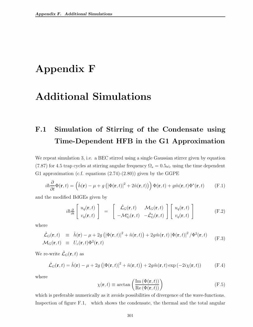
Appendix F. Additional Simulations
Appendix F
Additional Simulations
F.1 Simulation of Stirring of the Condensate using
Time-Dependent HFB in the G1 Approximation
We repeat simulation 3, i.e. a BEC stirred using a single Gaussian stirrer given by equation
(7.87) for 4.5 trap cycles at stirring angular frequency Ωs = 0.5ωr using the time dependent
G1 approximation (c.f. equations (2.74)-(2.80)) given by the GGPE
i~∂
∂tΦ(r, t) =
(
h(r)− µ+ g(
|Φ(r, t)|2 + 2n(r, t))
)
Φ(r, t) + gm(r, t)Φ∗(r, t) (F.1)
and the modified BdGEs given by
i~ ∂∂t
[
uq(r, t)
vq(r, t)
]
=
[
LG(r, t) MG(r, t)
−M∗G(r, t) −L∗
G(r, t)
][
uq(r, t)
vq(r, t)
]
(F.2)
where
LG(r, t) ≡ h(r)− µ+ 2g(
|Φ(r, t)|2 + n(r, t))
+ 2gm(r, t) |Φ(r, t)|2 /Φ2(r, t)
MG(r, t) ≡ Uc(r, t)Φ2(r, t)
(F.3)
We re-write LG(r, t) as
LG(r, t) = h(r)− µ+ 2g(
|Φ(r, t)|2 + n(r, t))
+ 2gm(r, t) exp (−2iχ(r, t)) (F.4)
where
χ(r, t) ≡ arctan
(
Im (Φ(r, t))
Re (Φ(r, t))
)
(F.5)
which is preferable numerically as it avoids possibilities of divergence of the wave-functions.
Inspection of figure F.1, which shows the condensate, the thermal and the total angular
301
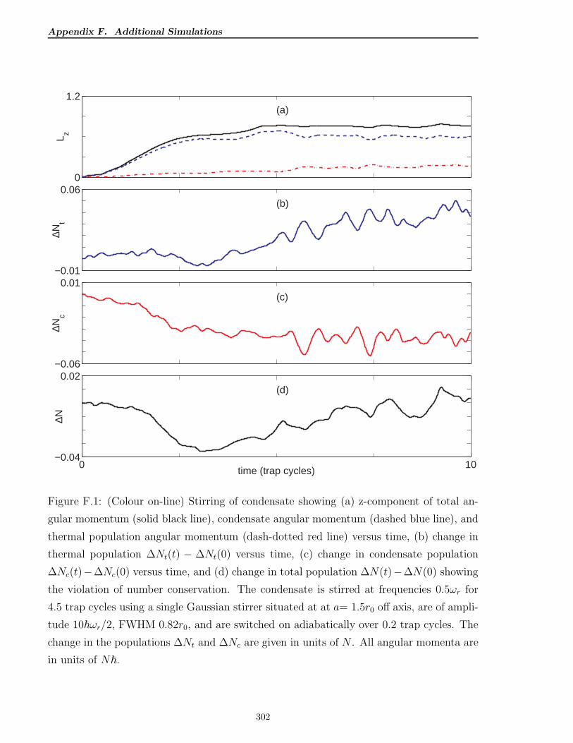
Appendix F. Additional Simulations
0
1.2
L z
(a)
−0.01
0.06
∆Nt
(b)
−0.06
0.01
∆Nc
(c)
0 10−0.04
0.02
time (trap cycles)
∆N
(d)
Figure F.1: (Colour on-line) Stirring of condensate showing (a) z-component of total an-
gular momentum (solid black line), condensate angular momentum (dashed blue line), and
thermal population angular momentum (dash-dotted red line) versus time, (b) change in
thermal population ∆Nt(t) − ∆Nt(0) versus time, (c) change in condensate population
∆Nc(t)−∆Nc(0) versus time, and (d) change in total population ∆N(t)−∆N(0) showing
the violation of number conservation. The condensate is stirred at frequencies 0.5ωr for
4.5 trap cycles using a single Gaussian stirrer situated at at a= 1.5r0 off axis, are of ampli-
tude 10~ωr/2, FWHM 0.82r0, and are switched on adiabatically over 0.2 trap cycles. The
change in the populations ∆Nt and ∆Nc are given in units of N . All angular momenta are
in units of N~.
302
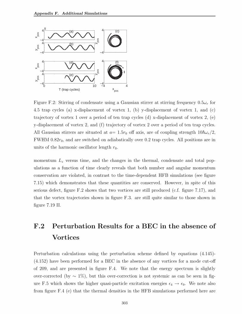
Appendix F. Additional Simulations
−4
4
x pos
II(a)
−4
4
y pos (b)
−4
4
x pos (d)
0 10−4
4
T (trap cycles)
y pos (e)
−4
4
y pos
(c)
−4 4−4
4
xpos
y pos
(f)
Figure F.2: Stirring of condensate using a Gaussian stirrer at stirring frequency 0.5ωr for
4.5 trap cycles (a) x-displacement of vortex 1, (b) y-displacement of vortex 1, and (c)
trajectory of vortex 1 over a period of ten trap cycles (d) x-displacement of vortex 2, (e)
y-displacement of vortex 2, and (f) trajectory of vortex 2 over a period of ten trap cycles.
All Gaussian stirrers are situated at a= 1.5r0 off axis, are of coupling strength 10~ωr/2,
FWHM 0.82r0, and are switched on adiabatically over 0.2 trap cycles. All positions are in
units of the harmonic oscillator length r0.
momentum Lz versus time, and the changes in the thermal, condensate and total pop-
ulations as a function of time clearly reveals that both number and angular momentum
conservation are violated, in contrast to the time-dependent HFB simulations (see figure
7.15) which demonstrates that these quantities are conserved. However, in spite of this
serious defect, figure F.2 shows that two vortices are still produced (c.f. figure 7.17), and
that the vortex trajectories shown in figure F.3. are still quite similar to those shown in
figure 7.19 II.
F.2 Perturbation Results for a BEC in the absence of
Vortices
Perturbation calculations using the perturbation scheme defined by equations (4.145)-
(4.152) have been performed for a BEC in the absence of any vortices for a mode cut-off
of 209, and are presented in figure F.4. We note that the energy spectrum is slightly
over-corrected (by ∼ 1%), but this over-correction is not systemic as can be seen in fig-
ure F.5 which shows the higher quasi-particle excitation energies ǫ4 → ǫ9. We note also
from figure F.4 (e) that the thermal densities in the HFB simulations performed here are
303
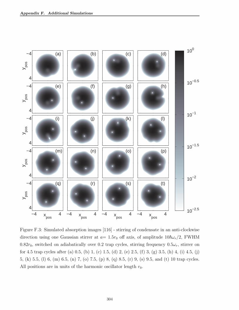
Appendix F. Additional Simulations
y pos
(a)−4
4
(b) (c) (d)
y pos
(e)−4
4
(f) (g) (h)
y pos
(i)−4
4
(j) (k) (l)
y pos
(m)−4
4
(n) (o) (p)
xpos
y pos
(q)
−4 4
−4
4
xpos
(r)
−4 4 xpos
(s)
−4 4 xpos
(t)
100
10−0.5
10−1
10−1.5
10−2
10−2.5
−4 4
Figure F.3: Simulated absorption images [116] - stirring of condensate in an anti-clockwise
direction using one Gaussian stirrer at a= 1.5r0 off axis, of amplitude 10~ωr/2, FWHM
0.82r0, switched on adiabatically over 0.2 trap cycles, stirring frequency 0.5ωr, stirrer on
for 4.5 trap cycles after (a) 0.5, (b) 1, (c) 1.5, (d) 2, (e) 2.5, (f) 3, (g) 3.5, (h) 4, (i) 4.5, (j)
5, (k) 5.5, (l) 6, (m) 6.5, (n) 7, (o) 7.5, (p) 8, (q) 8.5, (r) 9, (s) 9.5, and (t) 10 trap cycles.
All positions are in units of the harmonic oscillator length r0.
304
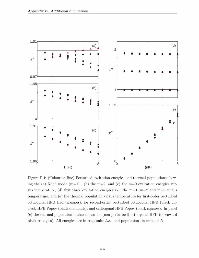
Appendix F. Additional Simulations
0.97
1.01
ε 1
(a)
1.4
1.48
ε 2
(b)
0 81.86
1.91
T(nK)
ε 3
(c)
1
2
ε q
(d)
0 80
0.25
T(nK)
Nt
(e)
Figure F.4: (Colour on-line) Perturbed excitation energies and thermal populations show-
ing the (a) Kohn mode (m=1) , (b) the m=2, and (c) the m=0 excitation energies ver-
sus temperature, (d) first three excitation energies i.e. the m=1, m=2 and m=0 versus
temperature, and (e) the thermal population versus temperature for first-order perturbed
orthogonal HFB (red triangles), for second-order perturbed orthogonal HFB (black cir-
cles), HFB Popov (black diamonds), and orthogonal HFB Popov (black squares). In panel
(e) the thermal population is also shown for (non-perturbed) orthogonal HFB (downward
black triangles). All energies are in trap units ~ωr, and populations in units of N .
305
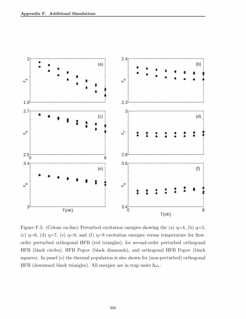
Appendix F. Additional Simulations
1.9
2
ε 4
(a)
2.3
2.4
ε 5
(b)
0 82.5
2.7
ε 6
(c)
2.8
3
ε 7
(d)
3
3.4
T(nK)
ε 8
(e)
0 83.4
3.6
T(nK)
ε 9
(f)
Figure F.5: (Colour on-line) Perturbed excitation energies showing the (a) q=4, (b) q=5,
(c) q=6, (d) q=7, (e) q=8, and (f) q=9 excitation energies versus temperature for first-
order perturbed orthogonal HFB (red triangles), for second-order perturbed orthogonal
HFB (black circles), HFB Popov (black diamonds), and orthogonal HFB Popov (black
squares). In panel (e) the thermal population is also shown for (non-perturbed) orthogonal
HFB (downward black triangles). All energies are in trap units ~ωr.
306
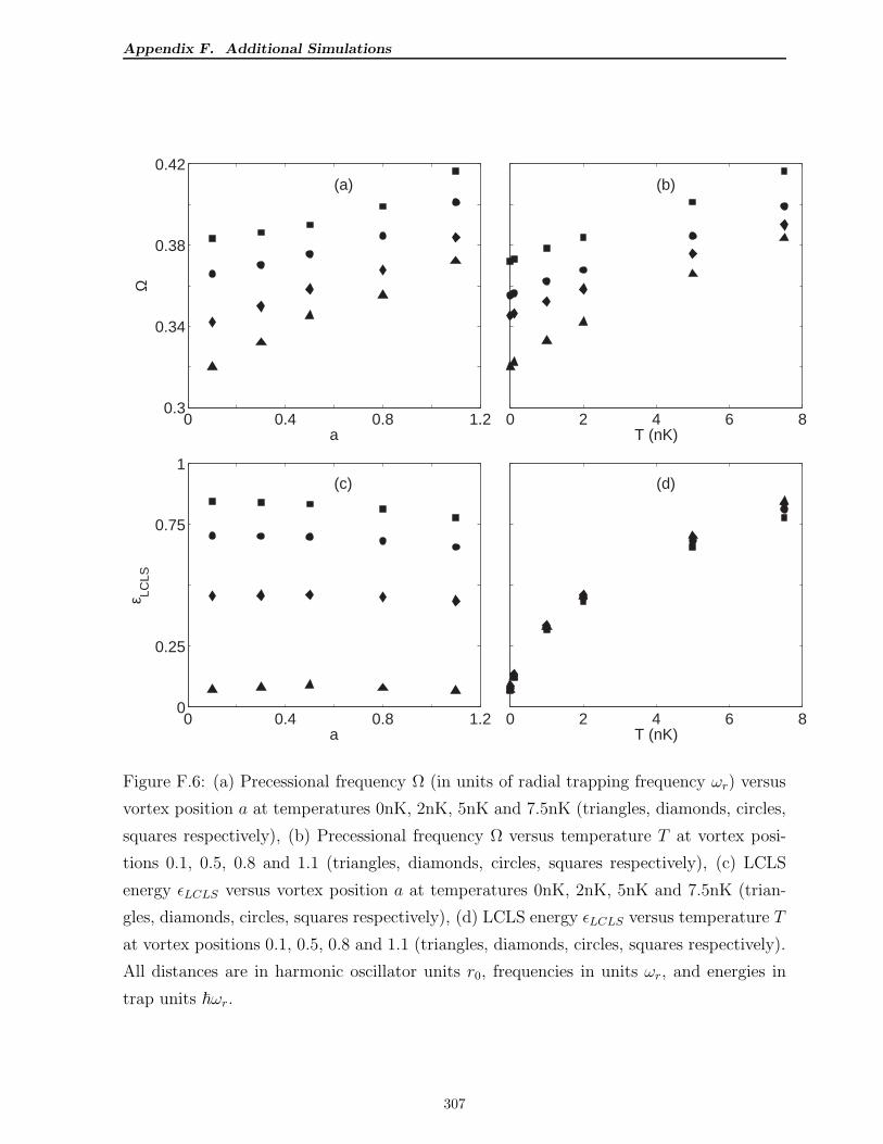
Appendix F. Additional Simulations
0 0.4 0.8 1.20.3
0.34
0.38
0.42
a
Ω
(a)
0 2 4 6 8T (nK)
(b)
0 0.4 0.8 1.20
0.25
0.75
1
a
ε LCLS
(c)
0 2 4 6 8T (nK)
(d)
Figure F.6: (a) Precessional frequency Ω (in units of radial trapping frequency ωr) versus
vortex position a at temperatures 0nK, 2nK, 5nK and 7.5nK (triangles, diamonds, circles,
squares respectively), (b) Precessional frequency Ω versus temperature T at vortex posi-
tions 0.1, 0.5, 0.8 and 1.1 (triangles, diamonds, circles, squares respectively), (c) LCLS
energy ǫLCLS versus vortex position a at temperatures 0nK, 2nK, 5nK and 7.5nK (trian-
gles, diamonds, circles, squares respectively), (d) LCLS energy ǫLCLS versus temperature T
at vortex positions 0.1, 0.5, 0.8 and 1.1 (triangles, diamonds, circles, squares respectively).
All distances are in harmonic oscillator units r0, frequencies in units ωr, and energies in
trap units ~ωr.
307
Appendix F. Additional Simulations
under-estimated by . 10% as alluded to earlier towards the end of chapter 4, but that this
should not qualitatively affect the results here.
F.3 The Effect of the Projection Operator P (r, r′, t) in
the GGPE in Orthogonal HFB on the Precession
of Off-Axis Vortices
The finite temperature time-independent calculations for off-axis vortices of section 7.4.3
in chapter 7 were repeated, now including the projection operator P (r, r′, t) in the GGPE
(4.106)
∆µΦ(r) =(
h(r)− µ+ g(
|Φ(r)|2 + 2n(r))
)
Φ(r)+ gm(r)Φ∗(r)−∫
dr′P (r′, r)φ(r′) (F.6)
in Orthogonal HFB equations (4.106), (4.107), and the results presented in figure F.6.
Comparing figures 7.5 and F.6 we notice that the results are quite similar for low T , but
exhibit an upward shift of ∼ 5-10% for higher temperatures.
308


![New efficient method for performing Hartree-Fock-Bogoliubov ...kenichi.matsuyanagi/PRC08a_Michel.pdf · Lagrangian [18] in the context of the relativistic Hartree-Bogoliubov theory](https://img.pdfslide.net/doc/110x75/60ea0b215285743bfb633121/new-eficient-method-for-performing-hartree-fock-bogoliubov-kenichimatsuyanagiprc08amichelpdf.jpg)


![Formation of Bose–Einstein condensates · Eckern developed a kinetic theory [12] for Hartree–Fock–Bogoliubov quasiparticles appropriate to the relaxation of the system on the](https://img.pdfslide.net/doc/110x75/5b33b7fb7f8b9a8b4b8b4a91/formation-of-boseeinstein-condensates-eckern-developed-a-kinetic-theory-12.jpg)