The Health Benefits of Solar Power Generation

FEBRUARY 2021 – EDF ECONOMICS DISCUSSION PAPER SERIES – EDF EDP 21–02

The Health Benefits of Solar Power Generation Evidence from Chile Nathaly M. Rivera, Cristobal Ruiz-Tagle, Elisheba Spiller

About Environmental Defense Fund

Guided by science and economics, Environmental Defense Fund (EDF) tackles our most urgent

environmental challenges with practical solutions. EDF is one of the world's largest

environmental organizations, with more than 2.5 million members and a staff of 700 scientists,

economists, policy experts and other professionals around the world.

EDF Economics Discussion Paper Series

EDF Economics Discussion Papers represent unrefereed works-in-progress by researchers who

are solely responsible for the content and any views expressed therein. Any comments on these

papers are welcome and should be sent to the author(s) by email. EDF’s Office of the Chief

Economist manages the series.

Sharing Our Discussion Papers

Our Discussion Papers (the “Materials”) are available for sharing and adaptation under an

Attribution-NonCommercial-NoDerivatives 4.0 International (CC BY-NC-ND 4.0) license (the

“License”). You can copy and redistribute the Materials in any medium or format; provided,

however: (i) you must give appropriate credit to us through recognition of our authorship of the

Materials (generally by citing to the Materials); (ii) you must provide the link to the License as

per the below; (iii) If you remix, transform, or build upon the Material, you may not distribute

the modified Material without our prior written consent; (iv) you may not apply any additional

restrictions to any third party that you distribute the Material to other then as specified herein,

except that you may not permit any third party to remix, transform or build upon the Materials,

without our prior written consent; and (v) you may not reproduce, duplicate, copy, distribute,

transmit, sell, trade, resell or exploit for any commercial purpose any portion of the

Materials. Images, trademarks, service marks, logos and icons used in the discussion papers are

our property and may not be used without our prior written consent. License information can be

found by visiting: https://creativecommons.org/licenses/by-nc-nd/4.0/

© 2021 Environmental Defense Fund. All rights reserved.

https://nam11.safelinks.protection.outlook.com/?url=https%3A%2F%2Fcreativecommons.org%2Flicenses%2Fby-nc-nd%2F4.0%2F&data=04%7C01%7Cespiller%40edf.org%7C30d3817e94a94a77c73c08d8c9f6d6d4%7Cfe4574edbcfd4bf0bde843713c3f434f%7C0%7C0%7C637481409292952331%7CUnknown%7CTWFpbGZsb3d8eyJWIjoiMC4wLjAwMDAiLCJQIjoiV2luMzIiLCJBTiI6Ik1haWwiLCJXVCI6Mn0%3D%7C1000&sdata=HUPZCjRzv4ChLjjAq6xZvo%2FnIgmf5sXo1pVROrT2%2BmM%3D&reserved=0

The Health Benefits of Solar Power Generation:

Evidence from Chile

Nathaly M. Riveraa, Cristobal Ruiz-Tagleb, Elisheba Spillerc

_____

a Corresponding author1. Department of Economics, University of São Paulo, [email protected] b Department of Geography and Environment, London School of Economics and Political Science, [email protected] c Environmental Defense Fund, [email protected]

Abstract

Renewable energy can yield social benefits through local air quality improvements and their

subsequent effects on human health. We estimate some of these benefits using data gathered

during the rapid adoption of large-scale solar power generation in Chile over the last decade.

Relying on exogenous variation from incremental solar generation capacity over time, we find

that solar energy displaces fossil fuel generation (primarily coal-fired generation) and curtails

hospital admissions, particularly those due to lower respiratory diseases. These effects are noted

mostly in cities downwind of displaced fossil fuel generation and are present across all age

groups. Our results document the existence of an additional channel through which renewable

energy can increase social welfare.

Key Words

Coal-fired power plants, coal displacement, solar generation, power plants, pollution, morbidity,

developing countries, Latin America

JEL Classification Numbers:

I18, L94, Q42, Q53

Acknowledgments:

We thank Andrew Bibler, Janet Currie, Harrison Fell, Maria Harris, Nicolai Kuminoff,

Lucija Muehlenbachs, Subhrendu K. Pattanayak, and Brett Watson and for helpful comments

1 Authors' contributions to the current version were as follows, with ~ denoting equal contribution. Conceptualization: NR~CR~BS. Methodology: NR, BS, CR. Data Curation: NR, CR, BS. Empirical Analysis: NR, BS, CR. Writing Original Draft: BS, NR.

mailto:[email protected]




and suggestions. We also thank seminar participants at Environmental Defense Fund,

Universidad Adolfo Ibañez, Universidad Católica del Norte, University of São Paulo, and

conference participants at the 21st Annual CU Environmental and Resource Economics

Workshop, the Association of Environmental and Resource Economists Annual Summer

Conference 2019, Camp Resources XXVI, Eastern Economic Association Annual Meeting 2020,

the 25th Annual Conference of the European Association of Environmental and Resource

Economists, and SETI Annual Meeting 2019, for helpful comments and suggestions. Any errors

are ours.

Contents

1 Introduction 6

2 Power Plants’ Emissions and Health Consequences 10

3 The Power Sector in Chile 11

3.1 The Generation Segment . . . . . . . . . . . . . . . . . . . . . . . . . . . . . 12

3.1.1 Solar Generation . . . . . . . . . . . . . . . . . . . . . . . . . . . . . 13

3.1.2 Emissions . . . . . . . . . . . . . . . . . . . . . . . . . . . . . . . . . 14

4 Data 16

4.1 Plant-Level Data . . . . . . . . . . . . . . . . . . . . . . . . . . . . . . . . . 16

4.2 Health Outcomes . . . . . . . . . . . . . . . . . . . . . . . . . . . . . . . . . 18

4.3 Wind Direction . . . . . . . . . . . . . . . . . . . . . . . . . . . . . . . . . . 20

4.4 Other Covariates . . . . . . . . . . . . . . . . . . . . . . . . . . . . . . . . . 20

5 Methods 21

5.1 Displacement . . . . . . . . . . . . . . . . . . . . . . . . . . . . . . . . . . . 21

5.2 Solar Generation and Health . . . . . . . . . . . . . . . . . . . . . . . . . . . 23

5.2.1 Air Pollution Exposure and Wind Direction . . . . . . . . . . . . . . 25

6 Results 26

6.1 Fossil Fuel Displacement . . . . . . . . . . . . . . . . . . . . . . . . . . . . . 26

6.2 Solar Generation and Health Outcomes . . . . . . . . . . . . . . . . . . . . . 30

6.2.1 Long-Term Health Effects . . . . . . . . . . . . . . . . . . . . . . . . 32

6.2.2 Fossil Fuel Generation, Pollution and Health in Chilean Cities . . . . 34

7 Robustness Checks 37

7.1 Alternative Groups of Cities . . . . . . . . . . . . . . . . . . . . . . . . . . . 37

7.2 Rate of Hospital Admissions . . . . . . . . . . . . . . . . . . . . . . . . . . . 39

7.3 Placebo Health Outcomes . . . . . . . . . . . . . . . . . . . . . . . . . . . . 40

8 Discussion 40

5

The Health Benefits of Solar Power Generation

1 Introduction

Renewable energy is the world’s fastest-growing energy source, set to become the leading

source of primary energy consumption by 2050 (U.S. Energy Information Administration,

2019). It promises several benefits to society, ranging from reductions in greenhouse gas

emissions, lower discharge of local air pollutants and improved health outcomes, to a re-

duced dependence on imported fuels and the creation of jobs through the manufacturing

and installation of these resources (U.S. Environmental Protection Agency, 2019). Yet, we

still lack a good understanding of the magnitude of some of these benefits, notably those

associated with health improvements. In this work, we use the rapid adoption of large-scale

solar power generation in the desert region of northern Chile to empirically quantify some

of the health benefits of solar energy.

Fossil fuel power generation, particularly that from coal combustion, releases large amounts

of local air pollutants, including sulfur dioxide (SO2), nitrogen oxides (NOX), mercury (Hg)

and particulate matter (PM). All of these pollutants are associated with several adverse

health effects, along with increased hospital admissions, mortality risks and threats to life

expectancy.1 The extent to which these emissions are curtailed with the introduction of

renewables reflects the potential of alternative energy sources to offset some of the negative

effects of dirty electricity generation. Nonetheless, some fossil fuel plants (e.g., natural

gas plants) have consistently been dispatched to deal with the intermittency of renewables

(Fell and Linn, 2013), thus attenuating the benefits of increasing the supply of these sources.

More insights on the co-benefits of renewable energy are, therefore, crucial to the cost–benefit

analyses of transitioning away from fossil fuels and, thus, for the optimal design of energy

policy.

The Atacama Desert, one of the sunniest and driest deserts in the world, not only has the

highest average surface solar radiation worldwide (Rondanelli et al., 2015), but also the

highest solar power potential. Figure 1 shows Chile’s photovoltaic power potential—a solar

energy system’s maximum productivity over time—relative to the rest of the world. This

potential, together with the recent decline in the cost of photovoltaic (PV) technology and

the country’s regulations aimed at fostering the adoption of renewables, resulted in rapid

market penetration of solar generation in Chile. By the end of 2012, a variety of solar plants

with capacity ranging from 3 MW to 138 MW were already injecting electricity into Chile’s

northern electric grid. We take advantage of this surge in large-scale investment in solar

energy to explore the effects of the steady expansion in solar capacity on generation from

1For comprehensive reviews, see Currie et al. (2014) on the effects of early-life exposure to pollution, andHoek et al. (2013) on the mortality impact of long-term air pollution exposure.

6

EDF Economics Discussion Paper 21-02

Figure 1: Chile’s Photovoltaic Power Potential (kWh/kWp)

Notes: Graph retrieved from https://globalsolaratlas.info. Solar resource data obtained from theGlobal Solar Atlas, owned by the World Bank Group and provided by Solargis. Photovoltaic power potentialrefers to how much energy (kWh) is produced per kilowatt peak (kWp) of a system.

thermal plants and on human health in northern Chile. By exploring the case of Chile, we

add to the scant literature on power plant pollution exposure and health impacts in emerging

economies (Gupta and Spears, 2017; Barrows et al., 2018).

Our study uses data on solar generation between 2012 and 2017. To identify the effects of this

increasing solar expansion, we first estimate the extent to which solar plants displace other

power facilities using daily variation in plant-level power generation capacity.2 For solar

generation to have a positive effect on health outcomes, it must first displace generation

by thermal plants.3 Next, we estimate a reduced form equation on the effect of daily solar

generation on health. In particular, we measure health effects using data on daily hospital

admissions of patients with health conditions generally associated with the combustion of

fossil fuels, and we estimate a set of zero-inflated negative binomial (ZINB) regressions that

relate daily solar variation to these admissions. Using limited data on fine PM concentrations,

we complement this analysis with an instrumental variable control function approach that

uses solar generation as an instrument for pollution in our health regressions. Throughout

all of our health equations, we indirectly take into account the transport of pollutants by

focusing on cities downwind of displaced fossil fuel plants.

2Ideally, we would use plant-level emissions data. Unfortunately, publicly available emissions data inChile are engineering estimates, rather than observed or measured data.

3The alternative is that solar generation rises to meet expanding demands for electricity. In this case, therewould be no displacement of fossil fuel plants, and the health impacts of the energy system would remainunchanged, although health improvements would have been seen relative to a counterfactual of increasedfossil fuel generation in response to increased loads.

7

https://globalsolaratlas.info


Our results show that increased solar generation in Chile led to a displacement of daily

thermal generation, particularly of coal- and gas-fired power generation. Subsequently, we

find that, through this displacement, solar generation reduces cardiovascular and respiratory

admissions in all cities included in our sample. Our analysis by age group indicates that

these reductions are mostly observed among infants, children (ages 6–14) and seniors, the

most vulnerable age groups. The reductions are found primarily after a short-term exposure

to abated pollution from displaced thermal plants, and in cities downwind of these displaced

facilities or that have fossil fuel generators within their borders. For cities closest to the

displaced plants, our results suggest that 1GWh of solar generation reduces all respiratory

hospitalizations by 52 per year, which represents a 13 percent reduction on average. These

conclusions remain unchanged after several robustness checks, which include the use of cities

upwind of displaced facilities and those downwind of nondisplaced units, and the use of

hospital admissions of patients with diseases presumably not related to air pollution.

Our findings can be considered a lower bound on the true health benefits from solar genera-

tion, particularly in developing countries. First, our area of study (Chile’s northern region)

has limited healthcare infrastructure, and thus any reduction in hospitalizations can have a

beneficial spillover effect in terms of increasing the number of hospital beds available, in turn

helping reduce the number of untreated unrelated injuries and illnesses. Second, reductions

in air pollution exposure for young children and infants has a lifelong benefit in terms of

reduced illnesses and improved economic outcomes (Currie et al., 2014). Third, the poor

and minorities may live closer to large air polluters in Chile, as has been demonstrated in

both the U.S. and India (e.g., Banzhaf et al. (2019); Kopas et al. (2020)). In this case,

improvements in air quality may not only bring greater long-term benefits on populations

experiencing uneven exposure to air pollution, but also help to reduce inequality.4

A wide number of papers document the displacement of coal-fired power plants, either

through a decline in the price of natural gas (Lu et al., 2012; Linn et al., 2014; Knittel

et al., 2015; Cullen and Mansur, 2017; Holladay and LaRiviere, 2017; Linn and Muehlen-

bachs, 2018), through the expansion in renewable generation capacity (Kaffine et al., 2013;

Cullen, 2013; Novan, 2015; Callaway et al., 2018; Fell et al., 2019), or through interaction

between the two (Holladay and LaRiviere, 2017; Fell and Kaffine, 2018). These studies also

document significant interactions among competing renewables, whereby solar generation

can lead to a shift in the supply of hydropower. To the extent that renewables offset and

4Previous evidence shows indications of population sorting in Chile in relation to other environmentaldisamenities, such as mining. For example, Rivera (2020) finds that residential properties near mining siteshave lower values and that these values are particularly salient for new residents in the area, suggesting anenvironmental-based sorting.

8


displace one another, the injection of new renewable sources into the grid may lead to am-

biguous environmental impacts. One of the benefits of conducting this analysis in northern

Chile is the small amount of non-solar renewables on the grid during the study period (they

made up only 6% of total capacity in 2017, combined). This allows us to isolate the effect

of solar generation on fossil fuel displacement more clearly.

We extend this previous literature by empirically documenting some of the consequences of

the displacement on morbidity outcomes. A small subset of literature estimates the effect

of changes in the power sector on health. For example, Burney (2020) estimates the health

benefits associated with the shift from coal to natural gas combustion in the U.S., finding

that the exit of coal-fired plants between 2005 and 2016 saved approximately 26,000 lives.

Along those lines, Casey et al. (2018a) find that coal and oil power plant retirement in

the U.S. led to improvements in fertility outcomes, and Casey et al. (2018b) show the link

between these retirements and a decrease in preterm births among nearby populations. Our

work adds to this literature, presenting new evidence on the benefits that curtailing coal-

fired generation has on morbidity. Moreover, we estimate this impact even without coal

plant retirement; rather, we are able to identify the health benefits of having a large amount

of solar generation at the intensive margin, even if it does not lead to coal plant shutdowns.

In doing so, we contribute to quantifying the value of curtailing coal-fired generation.

The analysis of solar generation also represents an advantage in evaluating the health ben-

efits of renewables relative to other similar sources such as wind. Increases in wind power

generation may be associated with reduced pollution due to higher wind speeds and greater

dispersion, hampering the identification of health impacts. There is existing work identifying

the health benefits of a cleaner grid (e.g., Anenberg et al. (2012); Muller and Mendelsohn

(2009)) or the addition of new utility-scale solar capacity (e.g., Sergi et al. (2020)) in inte-

grated assessment frameworks. The latter employ cutting-edge air transport and chemical

transformation models, but use existing epidemiological literature and underlying health and

population statistics to calculate the impact of policies on health. To the best of our knowl-

edge, we are the first to empirically test the impact of increased large-scale solar generation

on health. Therefore, our work also adds to the growing literature on the co-benefits of

renewable generation (e.g., Siler-Evans et al. (2013); Barbose et al. (2016); Buonocore et al.

(2016); Spiller et al. (2017); Millstein et al. (2017)), a key aspect in evaluating the economic

potential of renewable energy portfolios (Edenhofer et al., 2013; Wiser et al., 2017), and in

the design of health-based air quality regulations (Abel et al., 2018; Thakrar et al., 2020).

The remainder of our work proceeds as follows. Section 2 reviews the literature on the

health effects of power plant emissions, while Section 3 describes the power sector in Chile.

9


Section 4 documents the data, and Section 5 presents the empirical strategy. The results

and robustness checks are in Sections 6 and 7, respectively. Section 8 concludes.

2 Power Plants’ Emissions and Health Consequences

Fossil-fuel electricity generation accounts for a large share of greenhouse gas emissions, par-

ticularly carbon dioxide (CO2), an important contributor to global warming and climate

change (Stocker et al., 2013). The sector is also a major driver of outdoor air pollution, pri-

marily due to the burning of coal, which releases an important amount of airborne pollutants

such as SO2, NOX , Hg and PM. All of these pollutants are associated with adverse health

effects, mortality risks and threats to life expectancy (e.g., Chay and Greenstone (2003a,b);

Currie and Neidell (2005); Bateson and Schwartz (2007); Currie et al. (2009); Chen et al.

(2013); Arceo et al. (2016); Knittel et al. (2016); Schlenker and Walker (2016)). Coal com-

bustion also affects water quality. Ash released after coal combustion can end up in water

reservoirs, contaminating waterways and sources of drinking water (Carlson and Adriano,

1993). Here, we briefly summarize the evidence on the detrimental health impact of exposure

to the main pollutants from coal combustion. Evidence suggests that its displacement by

solar generation is expected to curtail mostly SO2, PM and NOX emissions.

SO2 is an invisible gas, part of the sulfur oxide (SOX) family of gases, formed when fuel

containing sulfur (e.g., coal, oil) is burned during metal smelting or other industrial pro-

cesses (U.S. Environmental Protection Agency, 2014). Exposure to high concentrations of

this pollutant is associated with eye, nose, and throat irritation, infectious complications of

chronic obstructive pulmonary disease, and rises in hospital admissions due to obstructions

of the lower airway such as asthma (World Health Organization, 2006). SO2 reacts with

other compounds in the atmosphere to form fine PM. Particulate matter is the general term

used to describe solid particles, dust and drops found in the air, all with different composi-

tions and sizes. Evidence on the health impact of exposure to coarse PM (PM10) and fine

PM (PM2.5) suggests detrimental effects on a variety of health outcomes, including respira-

tory diseases (Schwartz, 1996; Coneus and Spiess, 2010), cardiovascular diseases (Schwartz

and Morris, 1995; Brook et al., 2010; Franklin et al., 2015), low birth weight (Currie et al.,

2009; Coneus and Spiess, 2010; Currie and Walker, 2011), and infant mortality (Chay and

Greenstone, 2003a,b; Arceo et al., 2016; Knittel et al., 2016).

NOX are reactive gases, and include nitrogen dioxide (NO2), nitrous acid (HNO2) and nitric

acid (HNO3). Although mobile sources are responsible for the highest domestic anthro-

pogenic release of NOX into the atmosphere, stationary fossil fuel combustion represents a

10


significant portion of annual domestic NOX emissions. Evidence on outdoor exposure to

NOX indicates rises in asthma and bronchitis diagnoses in children (Orehek et al. (1976);

Pershagen et al. (1995); Chauhan et al. (2003); Gauderman et al. (2005)), and older popu-

lations (Schlenker and Walker, 2016). This pollutant can also react in the presence of heat

and sunlight in the atmosphere to create ground-level ozone, a harmful chemical associated

with lung diseases and premature deaths (Bell et al., 2004, 2005).

Hg is a toxic pollutant present in rocks, including coal in its natural state. Burning coal

releases Hg into the air, and it eventually settles into waterbodies through atmospheric

deposition. Once in the water, Hg is transformed by aquatic microbes into methylmercury

([CH3Hg]+), a poisonous form of mercury that accumulates in fish. Eating contaminated fish

is associated with cardiovascular diseases (Salonen et al., 1995; Guallar et al., 2002), and with

damage to the central nervous system in unborn (Clarkson, 1990). In the same way, high

blood Hg levels have been associated with elevated risk of IQ loss among children (Trasande

et al., 2005). Currently, coal-fired power plants represent the largest source of domestic

anthropogenic emissions of this global air pollutant (U.S. Environmental Protection Agency,

2015).

Evidence on the health impact of exposure to power plant pollution is limited within the

Chilean context. Epidemiological research from Ruiz-Rudolph et al. (2016) show significantly

higher rates of cardiovascular and respiratory hospital admissions in Chilean municipalities

that host power plants and other large-scale polluters. Yet, the authors fail to take into

account proximity to the pollution source, or the air transport of pollutants in the vicinity of

these facilities. This further highlights the importance of our work—identifying a causal im-

pact of exposure to power plant pollution on respiratory and cardiovascular hospitalizations

in Chile by relying on an exogenous source of variation: the incremental solar electricity

generation capacity over time.

3 The Power Sector in Chile

The electricity sector in Chile is composed of three different segments: generation, trans-

mission and distribution, all 100% privately owned. The sector is dominated by fossil fuels,

which account for 53% of total generation, followed by hydro with 28%. The fossil fuel

generation mix is primarily coal (40%), followed closely by natural gas (36%) and petroleum

(24%) (Comision Nacional de Energıa, 2018).

Before 2018, Chile’s electricity market featured four different electric systems (see Figure

2): two major interconnected systems, the Northern Interconnected System (Sistema In-

11


terconectado del Norte Grande — SING) and the Central Interconnected System (Sistema

Interconectado Central — SIC); and two additional minor grids, the Aysen Electric System

(Sistema Electrico de Aysen — SEA) and the Magallanes Electric System (Sistema Electrico

de Magallanges — SEM). The SING system, located in Chile’s northern region, has 5 GW of

installed capacity, 2.5 GW of peak load and more than 85% reliance on fossil fuel generation

(i.e., coal, natural gas and diesel). Although the northern region of Chile is relatively unpop-

ulated, with SING serving only 7% of the country’s total population, this region hosts most

of the large-scale copper mining companies that operate in the country, a sector character-

ized by its electricity-intensive production activities.5 Conversely, the SIC system, located

in central-south Chile and with 17 GW of total installed capacity and 7 GW of peak load,

relies heavily on hydro generation (around 35%) and serves 90% of the country’s population.

These two major grids, SING and SIC, began an interconnection process in November 2017

that resulted in a full integration by May 2019, thereby creating Chile’s National Electric

System (Sistema Electrico Nacional — SEN). In this paper, we focus on the period before

November 2017, thus avoiding any potentially confounding factors that may be associated

with the interconnection itself.

3.1 The Generation Segment

Chile’s current electric service legislation offers established competitive conditions in the

generation segment and maintains regulatory conditions for the transmission and distribution

segments. Generation at SING is characterized by a spot market, long-term forward contracts

and capacity payments. The spot market is a merit-order dispatch model that operates under

the coordination of the Economic Load Dispatch Center (Centro de Despacho Economico

de Carga — CDEC), which dispatches generators based strictly on their marginal cost at

every hour to meet the system’s load. The marginal cost of the system is set at every hour

by the CDEC and equals the cost of the most expensive unit being dispatched (Galetovic

and Munoz, 2011).6 This dispatch, determined by the regulator based on fuel costs, informs

our methodology in estimating the displacement of fossil fuel plants by solar generation.

Specifically, we incorporate relative costs of fossil fuels into our dispatch equation to control

for the market forces that will play a large role in determining dispatch and the ability of

solar to displace fossil fuel plants (see Section 5.1).

5During 2016, the copper industry consumed 50,578 TJ of electricity supplied by SING. This consumptionwas equivalent to more than 30% of SING’s installed capacity of 5 GW (data retrieved in May 2020 fromhttps://www.cochilco.cl).

6Regardless of whether generators are dispatched or not, each of these agents receives a monthly capacitypayment aimed at guaranteeing enough generation capacity to supply energy during times of peak demand.

12

https://www.cochilco.cl


Figure 2: Bulk Power Systems in Chile

Notes: Adapted from the National Energy Commission Monthly Report, December 2017. https://www.

cne.cl/wp-content/uploads/2015/06/RMensual_v201712.pdf

3.1.1 Solar Generation

Although numerous PV systems have existed in Chile since 2007, they were originally mostly

in the form of small-scale stand-alone systems and formed part of rural electrification pro-

grams (Haas et al., 2018). In 2008, however, the Chilean government established a quota

system for renewable energies; this currently requires that these sources account for 20% of

participation in the energy mix by 2025 (Ministry of Energy, 2013). This policy, in com-

bination with decreasing costs in PV technology, led to the installation in 2012 of the first

large-scale solar plant in northern Chile, La Huayca, adding 25.05 MW of gross capacity to

SING. By 2015, solar participation at SING reached 119 MW, equivalent to 2% of the total

daily generation of the system (≈.376 GWh), and by the end of 2017 it had grown to 655

MW, equivalent to 10% (≈1.5 GWh).7

7Data retrieved from the annual reports of Chile’s National Energy Commission (Comision Nacional deEnergıa — CNE), https://www.cne.cl/nuestros-servicios/reportes/informacion-y-estadisticas/

13

https://www.cne.cl/wp-content/uploads/2015/06/RMensual_v201712.pdf

https://www.cne.cl/wp-content/uploads/2015/06/RMensual_v201712.pdf

https://www.cne.cl/nuestros-servicios/reportes/informacion-y-estadisticas/


3.1.2 Emissions

Due to Chile’s heavy reliance on fossil fuels, the power sector accounts for approximately

40% of the nation’s total greenhouse gas emissions, which translates as 34,568.2 kt and 1.6

kt of carbon dioxide equivalent emissions (CO2e) due to CO2 and methane (CH4) discharges,

respectively (Chile Environmental Ministry, 2018). In terms of criteria air pollutants, the

sector accounts for more than 30% of the country’s total NOX and SO2 emissions, two haz-

ardous pollutants common to coal combustion (see Section 2). This situation is aggravated

by the longevity of some fossil fuel power plants, as older plants generally emit more. At

SING, for instance, some coal-fired generators are the oldest in the country, with ages that

in some cases exceed 50 years (Programa Chile Sustentable, 2017). Annual discharges from

the sector in this region are equivalent to 57% and 40% of Chile’s total SO2 and NOX emis-

sions, respectively (Chile Environmental Ministry, 2017), with concentration readings that

generally exceed life-threatening levels.

As an example, Figure 3 plots the hourly average SO2 (a) and NOX (b) concentrations in

Tocopilla, the city with the highest number of coal-fired power plants in SING, before (solid

line) and after (dashed line) the first solar connection, in 2012. As observed in both panels,

there is a clear decrease in hourly average concentrations of these two pollutants after the

introduction of large-scale solar installations in the system, although NOX levels decrease

much more drastically than SO2. To the extent that these reductions are effectively due to

the entry of new solar installations, Figure 3 anticipates the potential health benefits of a

cleaner grid. In any case, SO2 and NOX hourly averages in this city still exceed U.S. EPA

standards, currently set at 200 µg/m3 for 1-hour SO2 concentrations, and 100 ppb for NO2,

the most prevalent form of NOX in the atmosphere.

Regarding PM, Chile has relatively high daily average PM2.5 concentrations. For instance,

national annual average concentrations reached 21 µg/m3 in 2017, well above the World

Health Organization (WHO) guidelines (10 µg/m3 per year), which in the country’s north is

largely due to the region’s dependence on fossil fuel power generation (Chile Environmental

Ministry, 2017).8 Figure 4 shows daily average PM2.5 concentrations in Tocopilla between

2009 and 2019. As shown, concentrations have decreased over time but still exceed WHO

standards for 24-hour averages (25 µg/m3) during certain times of the year. This highlights

the importance that solar-powered electricity can play in reducing environmental-related

health concerns in areas with a heavy reliance on fossil fuels.

Preferably, the main hypothesis of this paper would be tested using data similar to those in

8The power sector is also the largest emitter of direct discharges of pollutants into the ocean and coastalwaters in Chile’s northern region (Chile Environmental Ministry, 2017).

14


(a) SO2 (b) NOX

Figure 3: Hourly Sulfur Dioxide (SO2) and Nitrogen Oxide (NOX) Concentrations in To-copilla

Notes: Hourly averages are obtained after controlling for a quadratic time trend. “Before the first solarconnection” includes observations between 2007 and 2011. “After the first solar connection” includes databetween 2013 and 2017. SO2 is measured in micrograms per cubic meter of air (µg/m3), and NOX in partsper billion (ppb).

Figure 4: Tocopilla’s Daily Average PM2.5 Concentrations

Notes: Reference line represents the World Health Organization’s 24-hour mean guideline of 25 µg/m3.Data from Tocopilla’s stations at the National Air Quality Information System (Sistema de InformacionNacional de Calidad del Aire — SINCA), https://sinca.mma.gob.cl

Figures 3 and 4. Unfortunately, however, we lack comprehensive city-level data on airborne

pollution for all the cities in our sample, as air quality monitoring stations in Chile are scarce

15

https://sinca.mma.gob.cl


for cities other than Santiago. We address this limitation with our displacement analysis.

Later in the paper, we do use the only available data on PM2.5 concentrations for some of

the cities in our sample as an additional test on our results (see Section 6.2.2).

4 Data

4.1 Plant-Level Data

We obtain comprehensive plant-level data on daily power generation from the National Elec-

tricity Coordinator (Coordinador Electrico Nacional — CEN), the national body in charge

of SING. Along with the information on generation, the data include specifics on plant-level

technology and capacity, which we later merge with data on fuel use and prices obtained

from the National Energy Commission (Comision Nacional de Energıa — CNE). As Novem-

ber 2017 was the month in which SING and SIC were first connected, our sample covers the

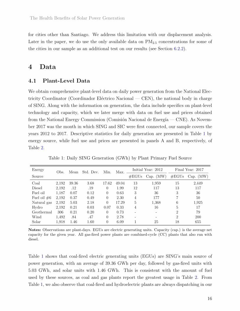
years 2012 to 2017. Descriptive statistics for daily generation are presented in Table 1 by

energy source, while fuel use and prices are presented in panels A and B, respectively, of

Table 2.

Table 1: Daily SING Generation (GWh) by Plant Primary Fuel Source

EnergyObs. Mean Std. Dev. Min. Max.

Initial Year: 2012 Final Year: 2017

Source #EGUs Cap. (MW) #EGUs Cap. (MW)

Coal 2,192 39.36 3.68 17.62 49.04 13 1,959 15 2,449Diesel 2,192 .12 .19 0 1.99 12 117 13 117Fuel oil 1,187 0.07 0.12 0 0.63 3 36 3 36Fuel oil #6 2,192 0.37 0.49 0 2.30 4 177 7 50Natural gas 2,192 5.03 2.18 0 17.29 5 1,368 6 1,925Hydro 2,192 0.21 0.03 0.07 0.33 4 16 5 17Geothermal 306 0.21 0.20 0 0.73 - - 2 79Wind 1,492 .84 .47 0 2.78 - - 2 200Solar 1,918 1.46 1.60 0 6.09 1 25 18 655

Notes: Observations are plant-days. EGUs are electric generating units. Capacity (cap.) is the average netcapacity for the given year. All gas-fired power plants are combined-cycle (CC) plants that also run withdiesel.

Table 1 shows that coal-fired electric generating units (EGUs) are SING’s main source of

power generation, with an average of 39.36 GWh per day, followed by gas-fired units with

5.03 GWh, and solar units with 1.46 GWh. This is consistent with the amount of fuel

used by these sources, as coal and gas plants report the greatest usage in Table 2. From

Table 1, we also observe that coal-fired and hydroelectric plants are always dispatching in our

16


Table 2: Monthly Fuel Use and Prices

Variable Mean Std. Dev. Min. Max. Obs.

Panel A. Fuel UseCoal 34,931.76 3,210.30 25,949.25 42,148.77 2,192Diesel 1,020.77 684.61 26.08 2,602.4 2,192Fuel oil 369.33 301.059 1 1,219 1,187Fuel oil #6 955.93 910.55 9 3,321.5 2,192Natural gas 15,333.87 7,389.24 3,371.79 44,707.66 2,192

Panel B. Fuel PricesCoal 105.41 16.21 68.19 138.73 2,192Diesel 620.94 200.63 288.5 908.7 2,192Fuel oil 95.79 22.91 46.67 125.33 1,187Fuel oil #6 446.96 175.40 157 728.41 2,192Natural gas 3.15 0.79 1.7 5.94 2,192

Notes: Using main fuel source only. Coal, diesel and fuel oil are in tons, while natural gas is in thousandsm3. Prices are in US$/ton for coal, US$/m3 for diesel and fuel oil #6, in US$/mm btu for natural gas, andin US$/bbl for fuel oil.

sample, as revealed by the positive minimum daily generation. Furthermore, solar generation

experienced the highest growth in terms of the number of new units and capacity installed

into the system, as shown in the last four columns of Table 1.9

Figure 5 depicts the share of SING’s monthly power generation by both fossil fuel and solar

facilities during the sample period. At the start of the period, power generation at SING was

(almost fully) coming from fossil fuels, with coal alone representing around 85% and natural

gas roughly covering the other 15%. Although there was some solar generation by the end

of 2012, a significant injection of solar-generated energy started at the beginning of 2015.

As shown in the same figure, this injection coincides with the persistent decrease in fossil

fuel power generation over the same period. By the end of 2017, coal-generated electricity

represented around 77% of SING’s monthly generation, while natural gas use was equivalent

to less than 10%.10

A more detailed overview of the relationship between solar and other fuels is offered by

Figure 6, which depicts SING’s hourly generation by fuel source averaged over the first week

9Note in Table 1 that the total net capacity of plants running with fuel oil #6 decreased from 177 MWin 2012 to 50 MW in 2017. This is due to the closure of two main generators, units U10 and U11, partof Termoelectrica Tocopilla, a power plant in operation since 1960. In fact, four generators were closedduring the sample period. Although solar generation may also displace fossil fuel generation at the extensivemargin, our main analysis is conservative as it is centered around the effects of displacement at the intensivemargin only. If these shutdowns were a consequence of the injection of solar power into the system, ourestimates would thus constitute a lower bound of the true effect of solar power generation on improvedhealth outcomes.

10Figure A1 in the Appendix shows SING’s daily load over the sample period. The increasing trend indemand over time indicated in this graph rules out a demand-driven reduction in fossil fuel power generation.

17


Figure 5: SING’s Monthly Fossil Fuel and Solar Power Generation

of January 2016 (left-hand side), and the last week of October 2017 (right-hand side), just

before the SING–SIC interconnection. Starting in 2016, SING had nine solar plants with

332 MW of total net capacity actively injecting power to the grid. By October 2017, this

capacity had doubled to 18 active solar projects, with a total net capacity of 654 MW. When

comparing these two periods in Figure 6, we observe that this increased solar capacity largely

displaced hourly coal- and gas-fired combustion during Atacama’s sunlight hours (7 a.m.–7

p.m.).

4.2 Health Outcomes

We use data from the Department of Health Statistics and Information (Departamento de

Estadısticas e Informacion de Salud — DEIS), part of Chile’s Ministry of Public Health,

from 2012 to 2017. DEIS provides data on each patient that has been discharged from any

hospital, together with information on their date of admission and the physician’s diagnosis

of the leading cause of disease. Although the data are compiled at the hospital or urgent care

center level, they include a variable on each patient’s city of origin, allowing us to match the

location of health outcomes with the location of generators. In our baseline specifications on

health, we look at daily hospital admissions at the city level as our main outcome. We focus

on hospital admissions due to cardiovascular and respiratory conditions, and, within respi-

ratory conditions, we further examine upper and lower respiratory infections.11 Descriptive

11Upper respiratory infections affect the nose and throat, causing symptoms such as sneezing and coughing.Among the most frequent upper respiratory infections are the common cold, sinusitis (sinus inflammation),

18


Figure 6: SING’s Hourly Generation by Fuel

Notes: Total hourly generation by fuel averaged over the first week of January 2016 (left-hand side), and thelast week of October 2017 (right-hand side). The left-hand side panel covers a period before the installationof nine additional solar projects, which subsequently doubled SING’s total solar installed capacity. By theend of 2017, just before the SING–SIC interconnection, SING’s total solar capacity had reached 654 MW(right-hand side).

statistics on hospital admissions by condition are presented in Table 3 for the 19 cities in

the sample.

Table 3: Descriptives on Daily Hospital Admissions

Disease Mean Std. Dev. Min. Max. Obs.

Cardiovascular 1.028 2.162 0 36 41,648All respiratory 1.070 2.346 0 25 41,648

Upper respiratory 0.331 1.092 0 16 41,648Lower respiratory 0.608 1.366 0 18 41,648

Notes: Observations are at the city level.

epiglottitis (trachea inflammation) and laryngitis (infection of the voice box). Lower respiratory infectionsaffect the lungs and lower airways. Common lower respiratory infections are bronchitis (bronchial tubeinflammation), bronchiolitis (an infection of the small airways, affecting children), pneumonia (a lung infec-tion), asthma (long-term disease of the lungs), influenza and tuberculosis (bacterial lung infection).

19


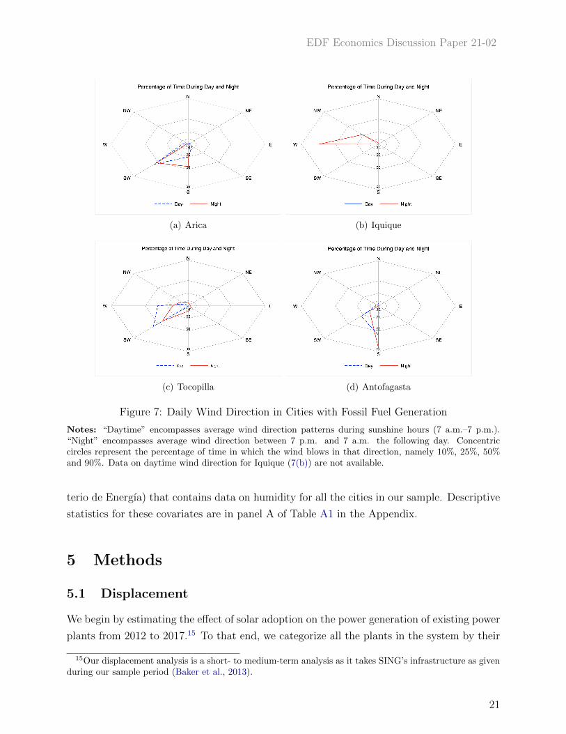
4.3 Wind Direction

Our data on wind direction come from Chile’s Meteorological Service and Air Quality System,

and cover four cities that host fossil fuel power plants, namely Arica, Iquique, Tocopilla and

Antofagasta. Mejillones also has a fossil fuel power plant but no available wind data; instead,

we rely on information from the nearest available city, Antofagasta, 62 km away. The eight-

wind compass roses for these cities are displayed in Figure 7 for daytime (dashed line) and

nighttime (solid line) wind patterns.12

Although wind speed is generally higher at night, we use daytime information given our

focus on the daily thermal displacement by solar energy sources. Considering that solar

installations produce at peak capacity around midday, we expect daytime wind direction

patterns to be more informative on a population’s true exposure to reduced emissions from

the displacement of fossil fuel generation during solar availability. Therefore, we obtain

average wind direction by drawing a pie slice with an angle of π/4 radians (i.e. 45 degrees)

bisected by average daytime wind direction in each location.13

4.4 Other Covariates

We also obtain information on other factors potentially correlated to hospital admissions.

First, we obtain data on city-level demographic characteristics such as population, density,

poverty and fertility rates as a proxy for socioeconomic factors known to affect health out-

comes.14 We gather this information from the National System of Municipalities Information

(Sistema Nacional de Informacion Municipal — SINIM). The demographic data are updated

every two years, and therefore we are able to include these variables in our estimation re-

gressions jointly with city-fixed effects.

Data on weather come from two different sources. First, we gather information on maximum

and minimum temperatures from the National System on Water Information (Sistema Na-

cional de Informacion del Agua — SNIA) for several monitoring stations located in remote

areas in northern Chile. Although we obtain this information for almost all cities in our

dataset, there are some incomplete entries, which we replace with daily regional averages.

The second source is Solar Explorer, an initiative of the Chilean Ministry of Energy (Minis-

12For the city of Iquique, we only have nighttime wind direction (see Figure 7(b)). In the definition ofdownwind cities, we approximate daytime wind patterns for this city using nighttime information.

13The resulting average wind direction is: 1.15π radians (206.9 degrees) in Arica (Figure 7(a)), 1.57πradians (282.7 degrees) in Iquique (Figure 7(b)), 1.33π radians (238.6 degrees) in Tocopilla (Figure 7(c)) and1.09π radians (196 degrees) in Antofagasta (Figure 7(d)).

14Unfortunately, city-level data on other indicators such as unemployment and income are not publiclyavailable.

20


(a) Arica (b) Iquique

(c) Tocopilla (d) Antofagasta

Figure 7: Daily Wind Direction in Cities with Fossil Fuel Generation

Notes: “Daytime” encompasses average wind direction patterns during sunshine hours (7 a.m.–7 p.m.).“Night” encompasses average wind direction between 7 p.m. and 7 a.m. the following day. Concentriccircles represent the percentage of time in which the wind blows in that direction, namely 10%, 25%, 50%and 90%. Data on daytime wind direction for Iquique (7(b)) are not available.

terio de Energıa) that contains data on humidity for all the cities in our sample. Descriptive

statistics for these covariates are in panel A of Table A1 in the Appendix.

5 Methods

5.1 Displacement

We begin by estimating the effect of solar adoption on the power generation of existing power

plants from 2012 to 2017.15 To that end, we categorize all the plants in the system by their

15Our displacement analysis is a short- to medium-term analysis as it takes SING’s infrastructure as givenduring our sample period (Baker et al., 2013).

21


primary fuel type (e.g., coal, diesel, natural gas, fuel oil) and then define a set of linear models

of daily generation to observe which types of plant decrease or increase their production with

the introduction of solar generation. Given our interest in the overall effect of solar power

generation on health, we use daily-level variation as our main specification because total

daily generation (and thus emissions) is more directly related to health outcomes than hourly

shifts. In particular, we define aggregated generation displacement equations as follows:

Gfd = γ0 + γ1Sd +

∑j 6=f

δj(FuelUsefm ∗

P fm

P jm

)+ γ2Loadd + ωd + τ + εfd , (1)

where Gfd is the system’s generation by fuel f during day d, ωd is a vector of daily weather

covariates, τ is a vector of time-fixed effects, and εfd is an error term. We consider two

variations of τ . The first of these, τ1, considers year, month, and weekend fixed effects, while

a stronger version, τ2, includes year, seasons, year × seasons, and weekend fixed effects.

Equation (1) also includes the variable Loadd that represents the system load during day d to

control for increases in demand over time, as demonstrated by Figure A1 in the Appendix.16

In addition, Equation (1) considers a term that models SING’s dispatch of generators to

control for differences in input prices that may affect daily dispatch conditions. This term

is given by the interaction between aggregate use of fuel f during month m, FuelUsefm, and

the relative international (exogenous) monthly prices of the fuels in the system, P fm/P j

m, where

f 6= j. Importantly, we do not include relative prices with respect to solar energy or other

renewables, given their zero marginal cost.

The key variable in Equation (1) is Sd, which represents the system’s solar generation during

day d. Whether solar power generation induces a significant displacement of non-solar sources

should be reflected by the displacement parameter γ1. We estimate Equation (1) with an

ordinary least square (OLS) estimator, bootstrapping the standard errors to account for

any heterogeneity and serial correlation in the generation data. To take into account the

heterogeneous capacity across fuel types, we also estimate an alternative specification of

Equation (1) in which we replace Gfd by capacity factor CF f

d , defined as total daily generation

by fuel f weighted by its net capacity. Given that CF fd takes values between 0 and 1, we

estimate this version of Equation (1) using a generalized least-squares (GLM) estimator

assuming a logit distribution.

In addition to the aggregated generation displacement, we run a plant-level version of Equa-

16As the large-scale copper mining industry is an important actor in the demand for energy at SING,variations in daily load should also capture similar variations in copper production.

22


tion (1) to identify the set of plants displaced by solar generation and those that are not. In

this case, we modify Equation (1) to include generation Gfid at the plant-level i, and their

corresponding fuel use FuelUsefim, as follows:

Gfid = β0 + β1Sd +

∑j 6=f

δj(FuelUsefim ∗

P fm

P jm

)+ β2Loadd + ωd + τ + εfid. (2)

5.2 Solar Generation and Health

Once we have confirmed that fossil fuel plants are indeed displaced by daily solar generation,

our next step is to estimate the resulting effect of solar power generation on health outcomes

(e.g., hospital admissions) for all cities in our sample, and for cities in close proximity to

these plants. A more in-depth discussion on this approach is offered in Section 5.2.1. We

define our baseline health equation as follows:

Healthjd = δ0 + δ1Sd + ωjd + ζ + τ + νjd, (3)

where Healthjd represents a health outcome in city j during day d; ωjd is a vector of daily

city-level weather covariates that may affect morbidity outcomes such as daily maximum and

minimum temperatures and humidity; ζ is a vector of demographics and city-fixed effects;

τ is a vector of time-fixed effects; and νjd is an idiosyncratic effect. As in Equation (1), we

consider two variations that include several combinations of weekend, month, season, and

year fixed effects.

The main variable in Equation (3) is Sd, which measures SING’s total solar generation on day

d. As we construct this variable considering all solar plants in the system, daily variation

in Sd is exogenous to any daily variation in hospital admissions in a given city j. Our

parameter of interest in Equation (3), δ1, gives us the marginal effect of solar generation

on the health outcome of interest. We estimate Equation (3) using a ZINB model due to

the large number of zeros in the outcomes (count variables) and a clear overdispersion of

these outcomes across cities in our sample.17 While we control for population in all of our

regressions, we also estimate Equation (3) with an OLS estimator on the rate of hospital

admissions per 100,000 people as a robustness check.18

17See Figure A2 (Appendix) for an example of two cities, Antofagasta and Tocopilla.18It is important to note here that some cities in northern Chile are very small in size, which means

that many of them report zero daily hospital admissions, particularly when it comes to admissions by agegroup. This complicates an OLS estimation on the rate of admissions, as in this case our outcome variableis continuous but with an important pileup at zero. Alternative estimation methods to deal with this, such

23


There are some potential drawbacks in the estimation of Equation (3). First, fossil fuel

plants are not randomly placed across the region, so cities with and without fossil fuel

plants may be observably different. Indeed, this is the case exhibited in panels B and

C of Table A1 (Appendix), which shows that cities without fossil fuel plants (panel C)

are smaller, less dense and poorer than those with fossil fuel plants (panel B) (all of these

differences are statistically significant). Thus, in addition to city-fixed effects, we also control

for demographic characteristics (e.g., poverty rate, density, fertility rate) in the estimation

of Equation (3). Second, the large copper mining industry is an important actor in the

demand on the energy sector in northern Chile, and also a significant air pollution emitter.

For this reason, we estimate an alternative specification to Equation (3) in which we control

for monthly large-scale copper production by city.19

Third, there may be important dynamic effects of daily avoided fossil-fueled pollution on

health outcomes. As air pollution gathers and accumulates in the atmosphere over time,

we would expect to see a lagged effect of daily improvements in air quality on health.20 In

particular, air quality improvements over three or four days may very well lead to greater

health benefits today than contemporaneous improvements in air quality. In that case,

Equation (3) would give us an incomplete picture of the actual health effect of a cleaner

grid.

There is precedent in the literature for testing the effect of lagged exposure to air pollution

on health. For instance, Neidell (2009) includes up to six days of lags, although the preferred

specification includes only four days, while Schlenker and Walker (2016) opt for three days

of lags. Although these two papers are looking at increases in air pollution, whereas our

method identifies the impact of air quality improvements, we could potentially identify a

dynamic effect through the inclusion of a couple of lags in our health equation. However,

this is not straightforward in our setting due to the fact that our main variable of interest

(solar generation) is highly colinear across days.21 Thus, including lags and leads would

result in unstable estimates due to the multicollinearity of the variables. Instead, we explore

a slightly different approach by testing whether there is a cumulative impact of longer-term

solar generation (and thus, longer periods of exposure to reduced fossil fuel-related pollution)

as a Hurdle estimation, resulted in the lack of convergence in many of our regressions.19We obtain this information from the Chilean Copper Corporation (Corporacion Chilena del Cobre —

COCHILCO). We would much rather use data on daily variation in production, but this information isunavailable.

20Indeed, there is evidence that certain air pollutants can have an extended effect on health. For instance,the U.S. Environmental Protection Agency (2006) found that ozone can have an effect on health for up tofour days after exposure.

21Our multicollinearity tests between Solard and Solard−l for l = {1, 2, 3} reveal variance inflation factors(VIFs) of magnitudes close to a 100.

24


on health. We do this by estimating the impact of average weekly, monthly, and yearly

solar generation on health outcomes, as depicted by Equation (4) where T = {7, 30, 365}.Expressed in this way, δt approximates the average long-term effect of solar generation on

daily hospital admissions.

Healthjd = δ0 + δtT−1

T∑t=1

Sd−t + ωjd + ζ + τ + νjd, (4)

5.2.1 Air Pollution Exposure and Wind Direction

A final concern regarding Equation (3) is that it ignores the potential air transport of pollu-

tants and, therefore, likely underestimates the effect on cities that are located closer to fossil

fuel plants and more exposed to their pollution, or displacement thereof. We address this

by rerunning our health equation using only those cities downwind of fossil fuel plants to

(indirectly) account for the transport of pollutants.22 To that end, we use the information

from the eight-wind compass roses in Figure 7, to guide us on exposure to pollution from

fossil-fueled generators.

Figure 8: Power Plant Locations in Tocopilla

Notes: Map of Tocopilla with the location of two fossil fuel power plants and the likely downwind areagiven the prevailing daytime wind direction.

For example, Tocopilla illustrates the case of a downwind city. From Figure 8, we can observe

that it hosts two power plants in its surrounding area, both at a distance of roughly 2 km and

22We state “indirectly” here because we do not have emissions data; thus, being downwind of a displacedplant only creates a proxy for potential to be in the line of emissions.

25


southwest from the city center.23 Combining this information with the prevailing wind at

this location (see Figure 7(c)), we observe that daytime wind blows from the southwest more

than 50% of the time, and from the west 40% of the time.24 Considering the location of the

thermal plants in Figure 8, it is straightforward to conclude that Tocopilla is downwind of

their emissions. Using similar information for all the cities that host thermal plants, we can

identify those that are downwind of thermal power generation. Furthermore, we combine

this information with the displacement results to construct an indicator for whether a city

is downwind of a displaced plant. In particular, we use four different categories throughout

the description of our health results: all cities, and cities downwind of displaced fossil fuel

plants that are located within 10km, within 50km or within 100km of their boundaries. In

addition, we can identify cities downwind of nondisplaced fossil fuel plants and those upwind

of displaced fossil fuel plants to use later in our robustness analyses.

6 Results

6.1 Fossil Fuel Displacement

Tables 4 and 5 present the results of the effect of 1-GWh of daily solar generation on the

displacement of daily aggregated generation (Equation (1)) for fossil fuels and renewable

sources, respectively. From left to right, each column shows a specification with more con-

trols. The two tables also include the effect of 1-GWh of daily solar generation on capacity

factors.

Our findings in Tables 4 and 5 suggest that solar-generated electricity displaces other fuel

sources, particularly dirty sources. From Table 4, we observe that a 1-GWh increase in daily

solar generation reduces the day-to-day generation of plants running with coal and with

natural gas by 0.48 and 0.27 GWh, respectively (columns 2).25 Considering the descriptive

statistics in Table 1, we observe that this displacement is roughly equivalent to 1.22% and

5.36% of the daily average power generated by these fossil fuels. Indeed, the results for

capacity factors in Table 4 show qualitatively similar results. An extra 1 GWh of solar

generation displaces 1.4 percentage points of the capacity factors of plants running with

coal, and 4.9 percentage points of the capacity factors of plants running with natural gas.

Table 4 suggests a ramp-up on capacity factors of plants running with diesel. Yet, this effect

23More specifically, at an angle of 217 degrees from the city’s geographical centroid.24Any other wind direction amounts to less than 5% during daytime.25Further analysis using simple cycle turbine plants reveals that solar energy displaces coal-fired single-

fuel engine generation at a larger magnitude (see Table A2 in the Appendix). This is an indication that thereduced coal use found in Table 4 is attenuated by dual-fuel engine coal-fired plants running with diesel.

26


Table 4: The Effect of 1 GWh of Solar Power Generation on Daily Aggregated Fossil FuelPower Generation

Coal Diesel Fuel oil Fuel oil #6 Natural gas

(1) (2) (1) (2) (1) (2) (1) (2) (1) (2)

Generation (GWh) -0.656∗∗∗ -0.483∗∗ 0.151 0.077 -0.011 -0.013 -0.016 -0.014 -0.215 -0.274∗∗

(0.175) (0.159) (0.094) (0.092) (0.019) (0.024) (0.017) (0.013) (0.150) (0.134)Capacity factor -0.021∗∗∗ -0.014∗∗∗ 0.015∗∗ 0.012 0.047 0.018 -0.018 -0.006 -0.063∗∗∗ -0.049∗∗∗

(0.003) (0.003) (0.006) (0.007) (0.041) (0.064) (0.012) (0.011) (0.009) (0.009)Obs. 1,915 1,915 1,915 1,915 910 910 1,915 1,915 1,915 1,915

Controls × × × × × × × × × ×τ1 fixed effects × × × × ×τ2 fixed effects × × × × ×

Notes: Marginal effects of 1 GWh of daily solar generation are derived from an OLS on daily aggregatedgeneration, and from a fractional logit response model on daily capacity factors. Estimations include plantswith both single- and dual-fuel engines. Controls include daily temperature, humidity, load and price ratios.Vector τ1 includes year, month, and weekend fixed effects. Vector τ2 includes year, seasons, year × seasons,and weekend fixed effects. Bootstrapped standard errors appear in parentheses. Significance levels: ∗p <0.10, ∗∗p < 0.05, ∗∗∗p < 0.001.

Table 5: The Effect of 1 GWh of Solar Generation on Daily Renewable Generation

Wind Hydro Geothermal

(1) (2) (1) (2) (1) (2)

Generation (GWh) 0.015 0.099∗∗∗ -0.008∗∗∗ -0.007∗∗∗ -0.071∗∗∗ -0.026(0.020) (0.019) (0.001) (0.002) (0.019) (0.016)

Capacity factor -0.004 0.013∗∗ -0.021∗∗∗ -0.018∗∗∗ -0.050∗∗∗ -0.040∗∗∗

(0.005) (0.004) (0.004) (0.005) (0.013) (0.011)Obs. 1,489 1,489 1,915 1,915 306 306

Controls × × × × × ×τ1 fixed effects × × ×τ2 fixed effects × × ×

Notes: Marginal effects of 1 GWh of daily solar generation are derived from an OLS on daily aggregatedgeneration, and from a fractional logit response model on daily capacity factors. Estimations include plantswith both single- and dual-fuel engines. Controls include daily temperature, humidity and load. Fuel priceratios are not included in this regression as these are renewable generators only. Vector τ1 includes year,month, and weekend fixed effects. Vector τ2 includes year, seasons, year × seasons, and weekend fixed effects.Bootstrapped standard errors appear in parentheses. Significance levels: ∗p < 0.10, ∗∗p < 0.05, ∗∗∗p < 0.001.

disappears once a stronger set of time-fixed effects is included.

The results for renewables in Table 5 suggest similar displacement effects on hydro, a dis-

patchable power source. In particular, the results in columns (2) indicate that, on average, a

1 GWh increase in daily solar generation displaces hydro by 0.007 GWh, equivalent to 3.3%

of the average hydro power generated in a single day. Regarding geothermal generation, we

find no effects, although the results on capacity factors indicate a significant reduction of

four percentage points. While this may be a weak effect, it is important to consider that the

27


geothermal displacement attenuates the potential benefits of a reduction in fossil fuels found

in 4. Because geothermal energy is a non-emitting source of electricity, its displacement will

reduce some of the health benefits associated with the expansion of solar generation. Hy-

dropower, on the other hand, is mostly utilized as a storage resource, dispatching in response

to high price times; thus, we are unable to directly identify the environmental impacts of

its displacement. Despite this potential attenuation, it is likely that the effect will be mi-

nor given the relatively small share of electricity that is produced by hydro and geothermal

sources (0.4% and 0.4% of mean daily generation, respectively; see Table 1). In summary,

we expect any attenuation effect from reduced hydro and geothermal generation to be small

compared to the benefits of displaced coal and natural gas, which account for 83% and 11%

of mean daily generation, respectively.

Finally, we find a positive coefficient of solar generation on wind generation, a non-

dispatchable (but curtailable) power source. The result for wind in column (2) of Table

5 indicates that a 1 GWh of daily solar generation ramps up wind generation by 0.099

GWh. Due to the non-dispatchability of wind generation, this likely reflects an underlying

correlation of wind and solar, given the thermally driven wind systems that characterize the

Atacama Desert (Jacques-Coper et al., 2015). Thermally driven winds are caused by local

differences in radiational heating and cooling systems, which in the case of the Atacama fa-

vor the complementarity between wind energy and solar energy (Jacques-Coper et al., 2015;

Munoz et al., 2018). An additional source of positive correlation between wind and solar

generation may come from the country’s effort to boost the adoption of renewable energy

sources, which has encouraged the installation of several wind parks in addition to solar

power plants (Ministry of Energy, 2013). In any case, given that wind generation is not

dispatchable but is curtailable, the fact that we are not getting a negative coefficient weakly

suggests that wind is not curtailed in response to greater solar output, or that, if curtailment

exists, it is not large enough to overcome the positive correlation between the two sources.

To delve deeper into the displacement of fossil fuel EGUs indicated in Table 4, Figure 9

plots the marginal effect of solar generation on daily generation levels and capacity factors

by coal-fired EGUs.26 Squares represent the point estimate of solar generation on daily coal

generation (left y-axis), and circles represent the marginal displacement of capacity factors

(right y-axis). We observe that the negative impact of solar generation on coal combustion

indicated in Table 4 is mostly explained by the shift in the generation of five units: U15,

U14, U12, CCR2 and CTA. Figure 9 also reveals the displacement of unit U13, statistically

26Similar graphs for diesel- and gas-fired units are provided in Figures A3 and A4, respectively, in theAppendix.

28


Figure 9: Coal-Fired EGUs and Displacement

Notes: The figure uses all EGUs that report coal (and its derivatives) as their primary fuel source. The lefty-axis shows the marginal effects of 1 GWh of daily solar generation on plant-level daily generation usingOLS. The right y-axis shows the marginal effects of 1 GWh of daily solar generation on daily capacity factorsusing a fractional logit response model. The estimation equation is identical to the one in columns (2) ofTable 4. Dashed lines represent 95% confidence intervals obtained with bootstrapped standard errors.

significant at the 10% level. Four of these units (U15, U14, U13 and U12) are part of the

Tocopilla coal-fired power station, which has been in operation since 1960 and is SING’s

oldest coal-fired plant.27 The largest generation displacement is found for the CTA unit that

belongs to the Atacama station. Power output for this unit decreased by 216 MWh, roughly

equivalent to 7% of its capacity. Considering this plant alone, this displacement translates

into more than 200 MWh of coal-fired generation avoided on a given day. This is closely

followed by reductions in CCR2’s output, one of the largest EGUs in the system (274.9

MW of gross capacity.28 On average, our estimates reveal that 1 GWh of solar generation

displaces 203 MWh of generation from the Atacama plant on a given day.

In addition to the displacement of several coal-fired units, Figure 9 also reveals a statistically

significant ramp-up in the power generation of two facilities: NTO1 and NTO2. On average,

1 GWh of daily solar generation increases generation in these plants by 90 and 89 MWh,

respectively, jointly equivalent to 0.46% of the daily coal-fired generation (see Table 1).

These two units are part of the Norgener power plant, also located in Tocopilla. Although

27At the time of writing, the Chilean government announced its plans to shut down these four unitsbetween 2019 and 2024. Source: Online. Retrieved: December 2019.

28Units CCR1 and CCR2 belong to the Cochrane Power Station, with more than 500 MW of gross capacity.

29

https://www.paiscircular.cl/industria/gobierno-anuncia-cierre-de-8-centrales-pero-deja-pendiente-cronograma-para-20-restantes-y-fija-en-21-anos-el-plazo-para-el-fin-del-carbon/


the ramp-up in the generation of these two coal-fired units is significantly lower than the

displacement found for other facilities, the increase slightly attenuates the plausible health

impact of the overall set of displaced plants in Tocopilla.

6.2 Solar Generation and Health Outcomes

The results on the effects of 1 GWh of solar generation on daily hospital admissions using

Equation (3) are displayed in Table 6 for cardiovascular and respiratory conditions. We

present these results using alternative groups of cities. Columns (1) and (2) both include

controls that capture weather conditions, city-level mining production and demographics.29

However, we vary the time-fixed effects across the two columns: columns (1) include year,

month and weekend fixed effects, while columns (2) have more expansive time-fixed effects,

including year, season, year season, and weekend fixed effects.

Table 6: The Effect of 1 GWh of Solar Generation on Hospital Admissions

All Cities Downwind of Displaced Fossil Fuel Plants

Cities < 10km < 50km < 100km

(1) (2) (1) (2) (1) (2) (1) (2)

Panel A. CardiovascularSolar -0.003 -0.025∗ -0.025 -0.061 -0.015 -0.037 -0.014 -0.022

(0.013) (0.014) (0.048) (0.070) (0.091) (0.040) (0.021) (0.015)Panel B. All respiratory

Solar 0.023 -0.060∗∗∗ -0.087 -0.142∗∗ -0.055 -0.092∗∗ -0.037 -0.078(0.020) (0.015) (0.071) (0.047) (0.047) (0.038) (0.040) (0.137)

Panel C. Upper respiratorySolar -0.07 -0.021∗∗ -0.037 -0.033∗∗∗ -0.024∗∗ -0.026∗∗∗ -0.023∗∗ -0.021

(0.019) (0.009) (0.075) (0.007) (0.012) (0.006) (0.009) (0.085)Panel D. Lower respiratory

Solar 0.022 -0.015 -0.064 -0.122∗∗∗ 0.005 -0.084∗∗∗ -0.010 -0.067∗∗∗

(0.014) (0.011) (0.049) (0.031) (0.034) (0.03) (0.032) (0.018)

Obs. 36,385 36,385 3,830 3,830 5,745 5,745 7,660 7,660Controls × × × × × × × ×City fixed effects × × × × × × × ×τ1 fixed effects × × × ×τ2 fixed effects × × × ×

Notes: Marginal effects from ZINB panel-data regressions using 100 iterations. Inflate regressions at countzero are estimated using a logit estimator. Controls include weather, mining production, and demographiccovariates (including population) in both the main and the inflate regressions. Vector τ2 includes year,seasons, year × seasons, and weekend fixed effects. Clustered standard errors by city appear in parentheses.Significance levels: ∗p < 0.10, ∗∗p < 0.05, ∗∗∗p < 0.001.

Altogether, the results indicate that solar generation leads to a reduction in hospital ad-

missions. For the full sample, we observe that 1 GWh of solar generation leads to a 0.025

29It is important to control for mining production as this sector is a significant polluter in the area andthe largest buyer of SING’s power. See Section 5 for more details.

30


average reduction in daily hospital admissions due to cardiovascular conditions, and to a

0.06 average reduction in admissions due to all respiratory conditions (columns (2)). To the

extent that emissions from displaced fossil fuel plants are not equally scattered across space,

these results are likely underestimating the effect of solar energy. Thus, to better understand

the effect of solar generation on health due to the displacement of emissions from dirty gen-

erators, we take into account the potential transport of pollutants and redefine our sample

to include cities downwind of displaced fossil fuel plants.

With this subsample, we obtain a stronger and larger effect in general admissions due to

respiratory conditions in the immediate vicinity of displaced plants (< 10km), although we

lose significance in cardiovascular conditions due to the reduction in statistical power. For

cities within 10km downwind of displaced plants, we observe that 1 GWh of daily solar

generation results in 0.142 fewer daily hospital admissions, or 52 fewer admissions per year

on average, due to all respiratory diseases, in cities near displaced fossil fuel power plants

(< 10km). Similar conclusions, albeit with decreasing magnitudes, are drawn for cities

within 50km and 100km of distance from displaced facilities.

Table 7: The Effect of 1 GWh of Solar Generation on Hospital Admissions by Age Group

All Cities Cities < 10km Downwind of Displaced Fossil Fuel Plants

Infants Toddlers Children Adults Seniors Infants Toddlers Children Adults Seniors

Panel A. CardiovascularSolar -0.00003 -0.0004 -0.001 -0.013∗ -0.004 -0.0003 -0.004 -0.001 -0.018 -0.020

(0.002) (0.036) (0.002) (0.008) (0.012) (0.001) (0.014) (0.006) (0.048) (0.028)Panel B. All respiratory

Solar -0.020∗∗ -0.010 -0.005 -0.005 -0.009∗∗∗ -0.048 -0.033 -0.003 -0.012 -0.013∗∗

(0.007) (0.011) (0.007) (0.005) (0.002) (0.092) (0.034) (0.456) (0.082) (0.006)Panel C. Upper respiratory

Solar -0.0001 -0.002 -0.011∗∗ -0.007∗ -0.001 -0.0001 -0.011 -0.005 -0.002 -0.001(0.001) (0.004) (0.005) (0.004) (0.001) (0.011) (0.144) (0.011) (0.059) (0.006)

Panel D. Lower respiratorySolar -0.012 -0.006 0.002 0.001 -0.002 -0.044 -0.022 -0.005 -0.008 -0.014

(0.012) (0.005) (0.009) (0.006) (0.004) (0.086) (0.065) (0.135) (0.134) (0.080)

Obs. 36,385 36,385 36,385 36,385 36,385 3,830 3,830 3,830 3,830 3,830Controls × × × × × × × × × ×City fixed effects × × × × × × × × × ×τ2 fixed effects × × × × × × × × × ×

Notes: Marginal effects from ZINB panel-data regressions using 100 iterations. Inflate regressions at countzero are estimated using a logit estimator. Controls include weather, mining production and demographiccovariates (including population) in both the main and the inflate regressions. Vector τ2 includes year,seasons, year × seasons, and weekend fixed effects. Clustered standard errors by city appear in parentheses.Significance levels: ∗p < 0.10, ∗∗p < 0.05, ∗∗∗p < 0.001.

We repeat the estimation of Equations (3) and (4) for different age groups using our strongest

specification (column (2) in Table 6). These results are given in Table 7 for all cities, and

for cities downwind of and within 10km of displaced fossil fuel power plants. The results

31


for cities downwind of displaced fossil fuel plants that are within 50km and 100km of their

limits are presented in Table A3 in the Appendix.

The results suggest that solar generation, through the displacement of fossil fuel energy, leads

to a positive effect in health outcomes across most age groups. Because we show the results

here for a limited sample of downwind cities, the number of observations in each age group

is significantly limited, thereby restricting the power of our estimation and reducing the

statistical significance. Thus, this regression of downwind cities identifies only statistically

significant improvements in all respiratory hospitalizations for seniors. However, when we

expand the buffer up to a distance of within 100km of a displaced fossil fuel plant, we find

reductions in respiratory hospitalizations for toddlers, children and seniors. We still do not

identify any statistically significant impact on cardiovascular hospitalizations.

6.2.1 Long-Term Health Effects

The results in Table 6 offer a general perspective of the net effect that day-to-day variation

in solar generation has on day-to-day variation in hospital admissions. Additional evidence

of the immediate co-benefit of solar is found in the results for Infants in Table 7, and in

Table A3. As stated in Currie and Neidell (2005), the link between cause and effect is

immediate in the case of infants, whereas diseases today in adults may reflect pollution

exposure from years ago. This immediate link is illustrated by the negative and statistically

significant effect of solar generation on hospital admissions of infants due to all respiratory

diseases found in panel B of Table 7. Comparable effects are found in panels B and D of

Table A3. Considering that infants are less than one year old, these findings corroborate the

contemporaneous aspect of the co-benefits of solar power generation.

To test whether these co-benefits also mask some permanent effects, we use the estimation

of Equation (4) where main explanatory variable is allowed to reflect the moving weekly,

monthly or yearly average solar generation in the system. Equation (4) also allows us to

take into account potential lagged effects of solar generation on contemporaneous health

outcomes, albeit indirectly. To that end, we express S = St, where t = {w,m, y}. Modeled

in this way, δt gives us the average marginal effect of 1 GWh of either weekly, monthly or

yearly average generation on daily relevant hospitalizations. The results using our strongest

specification are depicted in Table 8 for all ages, and in Table A5 by age group.

The results in Table 8 show the largest reductions in hospitalizations from weekly average

generation relative to those in columns (2) of Table 6, particularly for cities downwind of

nearby fossil fuel plants (< 10km). The fact that this coefficient is slightly greater than

32


the daily impact as reported in Table 6 suggests an additional effect of reduced cumulative

pollution exposure, although this added effect is present only in the relatively short term.

These cumulative effects, however, seem to be present in the relatively short term only,

as they become smaller and generally less significant as we move toward longer times of

exposure (monthly and yearly).

When exploring the results by age group in Table A5, we observe reductions in hospital

admissions of infants, children and seniors from weekly average generation. For instance,

for this last age group living in cities downwind of nearby thermal generation plants (<

10km), we observe a significant reduction of 0.025 in daily hospital admissions due to lower

respiratory diseases from weekly solar generation. Comparing this to the results in Table

7, we observe that the health effect of weekly solar generation for this age group is in line

with the presence of some cumulative effects but only in the short term, as it is significantly

greater than the effect of daily variation in solar power. Similar conclusions can be drawn for

infants and children. Taken together, the results in Tables 8 and A5 suggest that the average

health effects of exposure to reduced fossil fuel pollution are largely contemporaneous rather

than cumulative.

Table 8: The Long-Term Effect of 1 GWh of Solar Generation on Daily Hospital Admissions



t=week t=month t=year t=week t=month t=year t=week t=month t=year t=week t=month t=year

Panel A. CardiovascularSolart -0.043∗∗ -0.058 -0.097∗∗ -0.078 -0.112 -0.216 -0.050 -0.073 -0.146∗ -0.031∗ -0.034 -0.046

(0.015) (0.178) (0.036) (0.104) (0.118) (0.150) (0.057) (0.052) (0.083) (0.019) (0.035) (0.074)Panel B. All respiratory

Solart -0.090∗∗∗ -0.054∗∗ -0.026 -0.177∗∗ -0.084∗∗ 0.068 -0.116∗∗ -0.055 0.041 -0.094∗∗ -0.052∗∗ 0.024(0.014) (0.018) (0.044) (0.067) (0.027) (0.049) (0.039) (0.056) (0.027) (0.036) (0.024) (0.016)

Panel C. Upper respiratorySolart -0.019 -0.019 -0.022 -0.046∗∗∗ -0.016 0.011 -0.030 -0.013 -0.0002 -0.025∗∗ -0.014 -0.004

(0.012) (0.019) (0.025) (0.010) (0.038) (0.043) (0.019) (0.427) (0.029) (0.010) (0.145) (0.198)Panel D. Lower respiratory

Solart -0.016 -0.005 0.009 -0.137∗ -0.073 0.067 -0.101∗∗ -0.056 0.032 -0.081∗∗ -0.046 0.024(0.017) (0.015) (0.034) (0.071) (0.091) (0.127) (0.044) (0.052) (0.080) (0.035) (0.042) (0.054)

Obs. 36,366 36,366 36,366 3,828 3,828 3,828 5,742 5,742 5,742 7,656 7,656 7,656Controls × × × × × × × × × × × ×City fixed effects × × × × × × × × × × × ×τ2 fixed effects × × × × × × × × × × × ×


33


6.2.2 Fossil Fuel Generation, Pollution and Health in Chilean Cities

Our previous health results consistently show significant reductions in pollution-related hos-

pital admissions due to variation in solar power generation in Chile. Additionally, these

reductions are found mostly in cities downwind of fossil fuel plants that are displaced by so-

lar generation as revealed by our plant-level displacement analysis. While this strategy helps

us to take into account the air transport of pollutants emitted by thermal plants affected

by the injection of new solar power generation into the grid, it constitutes an indirect test

of the mechanism through which solar generation affects health. In this section, we explore

a more direct test on the mechanism through which solar generation is positively affecting

pollution-related admissions by using available data on PM2.5 concentrations for some of the

cities in our sample. As mentioned in Section 3.1.2, pollution data in Chile is scarce for

cities other than Santiago, yet we are able to gather data for some of the cities with fossil

fuel generation, and cities downwind of displaced fossil fuel plants.30 With these data, we

first test the link between thermal generation and air pollution concentrations, estimating

the effect of daily fossil fuel generation (i.e., coal, diesel and natural gas) on daily PM2.5

concentrations (in logs) as follows:

log(PM2.5)jd = ρ0 + ρ1Coaljd + ρ2Dieseljd + ρ3NaturalGasjd + ωjd + ζ + τ + υjd, (5)

where ωjd is a vector of daily city-level weather covariates (including wind speed, also avail-

able for these cities); ζ is a vector of demographics, mining production and city-fixed effects;

τ is a vector of time-fixed effects; and υjd is an idiosyncratic error. In an alternative spec-

ification, we replace thermal power for system-level daily solar generation. We estimate

Equation (5) with OLS using Newey–West standard errors to control for potential autocor-

relation known to affect pollution data.

The results for the strongest specification in columns (2) of Table 9 show that 1 GWh of

coal-fired generation increases PM2.5 concentrations by 1% in all cities for which we have

data. This effect becomes stronger and highly significant when looking at cities downwind

of fossil fuel plants. Specifically, 1 GWh of coal generation increases concentrations of PM2.5

by 2%, while 1 GWh of natural gas generation does so by 1%.31 Considering that daily

average concentrations of this pollutant are roughly 14.73 µg/m3 across cities with data,

30Specifically, we have data for Arica, Antofagasta, Tocopilla and Alto Hospicio. The last two cities,namely Tocopilla and Alto Hospicio, are part of the group of cities within 10km downwind of displaced fossilfuel plants. Pollution data was gathered from https://sinca.mma.gob.cl.

31As mentioned in our displacement analysis, all gas-fired plants in our sample are combined-cycled plantsthat operate with diesel as well, so this effect is likely due to the use of diesel in gas-fired plants.

34

https://sinca.mma.gob.cl


Table 9: The Effect of 1 GWh of Power Generation on Daily Log PM2.5

All Cities < 10km Downwind ofCities Displaced Fossil Fuel Plants

(1) (2) (1) (2) (1) (2) (1) (2)

Coal 0.007 0.014∗∗ 0.011∗∗ 0.020∗∗∗

(0.005) (0.005) (0.005) (0.006)Diesel -0.043 0.091 -0.138 -0.003

(0.105) (0.104) (0.126) (0.123)Natural Gas 0.006 0.009 0.009 0.011∗

(0.005) (0.06) (0.006) (0.006)Solar 0.007 -0.033∗∗ -0.019 -0.043∗∗

(0.013) (0.013) (0.016) (0.019)

Obs. 5,582 5,582 5,319 5,319 2,592 2,592 2,329 2,329Controls × × × × × × × ×City fixed effects × × × × × × × ×τ1 fixed effects × × × ×τ2 fixed effects × × × ×

Notes: Marginal effects from an OLS regression using Newey–West standard errors (in parentheses) allowingfor up to three lags. Controls include weather (min. and max. temperature, humidity and wind speed),mining production and demographic covariates (including population). Vector τ1 includes year, month, andweekend fixed effects. Vector τ2 includes year, seasons, year × seasons, and weekend fixed effects. Significancelevels: ∗p < 0.10, ∗∗p < 0.05, ∗∗∗p < 0.001.

these effects are equivalent to 0.295 and 0.147 µg/m3 daily increases in PM2.5. These results

are consistent with our previous findings on the displacement of coal-fired and gas-fired

facilities. Yet, they should be taken with caution as they cover the period between 2012 and

2017, already treated with the injection of solar generation, which may explain the reduced

magnitude of the coefficients. When replacing thermal generation with solar generation,

we find consistent and significant results. The results in columns (2) of Table 4 indicate

that 1 GWh of solar generation reduces PM2.5 concentrations by 3–4%. Altogether, the

findings in Table 4 indicate that thermal generation effectively increases airborne pollution

concentrations, while solar generation has the opposite effect.

Our final exercise considers the information in Table 4 in tandem with our health analysis. To

that end, we follow two approaches. First, we re-estimate our baseline ZINB health equations,

replacing the solar generation variable with city-level daily average PM2.5 concentrations. In

doing this, we have to consider that pollution-related hospital admissions are likely not

orthogonal to PM2.5 concentrations. For instance, PM2.5 can be formed due to chemical

reactions of secondary particles from SO2 and NOX , pollutants that are also common to coal

combustion and have a direct impact on health as well (World Health Organization, 2006).

In addition, other factors such as economic conditions may have a simultaneous impact on

both health outcomes and air pollution concentrations. Thus, while informative, omitted

35


factors in this regression may give us an inconsistent estimate of the impacts of pollution on

health.

Table 10: The Effect of Daily PM2.5 on Daily Hospital Admissions

All Cities < 10km Downwind ofCities Displaced Fossil Fuel Plants

ZINB CF ZINB CF

Panel A. CardiovascularPM2.5 -0.003 -0.006 -0.001∗∗∗ 0.020

(0.007) (0.023) (0.0004) (0.021)v 0.005 -0.023

(0.024) (0.022)Panel B. All respiratory

PM2.5 0.008 0.053∗∗ 0.009∗∗∗ 0.073∗

(0.009) (0.021) (0.002) (0.041)v -0.050∗∗ -0.069∗

(0.021) (0.042)Panel C. Upper respiratory

PM2.5 -0.002 0.002 0.002 0.005(0.006) (0.011) (0.002) (0.017)

v -0.006 -0.003(0.014) (0.012)

Panel D. Lower respiratoryPM2.5 0.012∗∗∗ 0.034 0.007∗∗ 0.059∗∗

(0.004) (0.029) (0.003) (0.021)v -0.024 -0.054∗∗

(0.027) (0.021)

First Stage (Solar) -0.600∗∗∗ -0.900∗∗∗

(0.120) (0.232)Obs. 5,319 5,319 2,329 2,329Controls × × × ×City fixed effects × × × ×τ2 fixed effects × × × ×

Notes: Marginal effects from both ZINB and CF ZINB regressions. PM2.5 is measured in µg/m3. v arethe residuals from the estimation of Equation (5). Controls include weather (min and max temperature,humidity and wind speed), mining production and demographic covariates (including population). Vector τ2includes year, seasons, year × seasons, and weekend fixed effects. Clustered standard errors by city (ZINB)and boostrapped standard errors (CF) appear in parentheses. Significance levels: ∗p < 0.10, ∗∗p < 0.05,∗∗∗p < 0.001.

The results on the health effects of PM2.5 are depicted in the ZINB column in Table 10 for

all cities and downwind cities. In line with our previous analyses, we observe that 1 µg/m3

of PM2.5 concentrations increases daily lower respiratory admissions in all cities, and all

respiratory and lower respiratory admissions in downwind cities. We also observe counterin-

tuitive, negative results for cardiovascular admissions in downwind cities, a result plausibly

explained by the endogeneity of our main explanatory variable. We solve this issue in a

second strategy, in which we use day-to-day variation in solar generation in an instrumen-

tal variable approach that uses a control function (CF) estimation (Wooldridge, 2015). We

adopt this two-step estimation given the non-linear distribution of the dependent variable

36


in the health equations, our second-stage equations.32 We carry out this CF exercise using

Equation (5) (unlogged) in a first-stage estimation with solar generation as the instrument,

and computing the residuals vjd that we include as an additional regressor in the estimation

of Equation (3) that uses PM2.5 as the main explanatory variable. A statistically significant

second-stage control function coefficient vjd constitutes a simple test on the endogeneity of

PM2.5 (Wooldridge, 2010), and can be interpreted as the effect of solar on health outcomes

through reductions in PM2.5. We present these results in column CF of Table 10, with

bootstrapped standard errors.

Daily variation in PM2.5 is found to increase daily respiratory admissions for all cities in our

sample. Additionally, a statistically significant estimate for vjd corroborates the endogeneity

of PM2.5, which may explain the lack of significance of this estimate in the previous ZINB

regression, or its counterintuitive signs. In fact, the negative vjd coefficient suggests that solar

generation effectively reduces the impact of PM2.5 on all hospital admissions, particularly all

respiratory admissions. We find consistent results when restricting the sample to downwind

cities. In this case, the CF results indicate a positive effect of PM2.5 on daily respiratory and

lower respiratory admissions, results that are almost fully mitigated by the injection of solar

generation. We take the results in Tables 9 and 10 as strong evidence that the co-benefits

of solar power generation on hospital admissions found throughout our analysis are largely

due to reductions in airborne pollution from displaced thermal generation.

7 Robustness Checks

7.1 Alternative Groups of Cities

Our results are robust to several alternative specifications. First, we check the robustness

of our wind direction analysis by splitting the sample between cities with and without fossil

fuel plants as an approximation to cities with and without pollution exposure. From our

displacement analysis, we are also able to consider cities that are downwind of fossil fuel

plants that were not displaced by the addition of solar generation into the grid, and cities

upwind of the displaced ones. We present these results in Table 11 using our strongest

specification.

Splitting the sample in this manner reveals that reductions in hospitalizations attributable

to solar generation are primarily found in places with fossil fuel generation. The results in

the first two columns of Table 11 suggest that additional solar generation predominantly

32See E.G., Kline and Walters (2016) for a recent example on the use of a control function approach.

37


Table 11: The Effect of 1 GWh of Solar Generation on Hospital Admission Using AlternativeGroups of Cities

With Without Downwind of Upwind ofFossil Fuel Fossil Fuel Nondisplaced NondisplacedGeneration Generation Fossil Fuel Plants Fossil Fuel Plants

Panel A. CardiovascularSolar -0.051 -0.015 0.007∗∗ -0.0003

(0.054) (0.010) (0.003) (0.002)Panel B. All respiratory

Solar -0.215∗ -0.023 -0.025 -0.002(0.127) (0.021) (0.076) (0.005)

Panel C. Upper respiratorySolar -0.093 -0.005 -0.003 -0.0002

(0.166) (0.006) (0.007) (0.003)Panel D. Lower respiratory

Solar -0.111∗∗∗ -0.007 -0.008 0.001(0.029) (0.008) (0.165) (0.002)

Obs. 9,575 24,895 3,830 7,660Controls × × × ×City Fixed Effects × × × ×τ2 × × × ×

Notes: Marginal effects from ZINB panel-data regressions using 100 iterations. All regressions includeweather covariates, season, year, weekend, city-fixed effects, demographics (e.g., density, fertility rate andpoverty rate) and mining production, in both the main and the inflate regressions. Inflate regressions atcount zero are estimated using a logit estimator. Clustered standard errors by city appear in parentheses.Significance levels: ∗p < 0.10, ∗∗p < 0.05, ∗∗∗p < 0.001.

curtails lower respiratory admissions in cities where displacement is possible. Namely, an

additional 1 GWh of solar generation results in 0.111 fewer daily lower respiratory admissions

in cities that house fossil fuel plants, roughly equivalent to 59 fewer yearly hospitalizations.

We do not find a statistically significant impact on hospitalizations for upper respiratory or

cardiovascular-related conditions, likely due to the failure to account for pollution transport.

We do find, however, a small but positive significant impact on cardiovascular hospitalizations

in cities downwind of nondisplaced fossil fuel plants. Namely, a 1 GWh of solar generation

is found to increase by 0.007 the number of daily hospital admissions due to cardiovascular

diseases. This is certainly an unexpected result, but it is important to point out that this

subsample includes only two cities, Sierra Gorda and Mejillones, and that the latter hosts all

gas-fired plants. Although our aggregated displacement analysis reveals that solar generation

displaces gas-fired generation, our plant-level analysis shows that one gas-fired unit ramps up

its production in response to the injection of this renewable (see Figure A4 in the Appendix).

Thus, a plausible explanation is that some pollution from this power plant reaches parts of

this city, even though it is downwind of nondisplaced plants. While we do not explore this

possibility further in the paper, it is important to note that this effect is small in magnitude

38


relative to those for cities with fossil fuel generation.33 Finally, and in contrast to our findings

in Table 6 for downwind cities, we find no statistically significant effects in cities upwind of

displaced fossil fuel plants.

7.2 Rate of Hospital Admissions

We also estimate an alternative version of our health equation using the rate of hospital

admissions per 100,000 people as the outcome variable. We present the OLS results for our

strongest health specification in Table 12. We find similar magnitudes of reduced hospital-

izations across all cities, although we lose significance when subsampling to downwind cities

alone. Here, it is important to consider that we have many small cities in our sample, which

translates into an abundant number of observations with zero daily hospital admissions. Ide-

ally, our OLS estimations using rate of admissions would account for this large number of

zeros in the data, yet that is not the case. While the OLS results on the rate of admissions

in Table 12 are useful as a first approximation, we take them with caution given the skewed

distribution of this dependent variable.

Table 12: The Effect of 1 GWh of Solar Generation on the Rate of Hospital Admissions



Panel A. CardiovascularSolar -0.004 -0.042 -0.043 -0.020

(0.041) (0.116) (0.065) (0.048)Panel B. All respiratory

Solar -0.116∗∗ -0.329 -0.192 -0.253(0.054) (0.273) (0.201) (0.154)

Panel C. Upper respiratorySolar -0.027 -0.078 -0.044 -0.053

(0.020) (0.065) (0.045) (0.032)Panel D. Lower respiratory

Solar -0.086∗∗ -0.269 -0.160 -0.193(0.041) (0.232) (0.169) (0.122)

Obs. 36,328 3,824 5,736 7,648Controls × × × ×City Fixed Effects × × × ×τ2 × × × ×

Notes: Marginal effects from OLS panel-data regressions. Controls include weather, mining productionand demographic covariates (including population) in both the main and the inflate regressions. Vector τ2includes year, seasons, year × seasons, and weekend fixed effects. Clustered standard errors by city appearin parentheses. Significance levels: ∗p < 0.10, ∗∗p < 0.05, ∗∗∗p < 0.001.

33We cannot estimate our health equations for cities downwind of the few plants ramping up their genera-tion in response to solar generation because, simultaneously, these cities are also downwind of some displacedfossil fuel plants.

39


7.3 Placebo Health Outcomes

Additionally, we test whether solar generation affects health outcomes that are, presumably,

unrelated to pollution. Table 13 displays the ZINB results of this falsification test using

infections(panel A), type 1 diabetes (panel B) and blood diseases (excluding anemia) (panel

C). We also include Schlenker and Walker (2016)’s placebo outcomes: strokes (panel D),

bone fractures (panel E) and appendicitis (panel F).34 The placebo results are all small and

statistically insignificant, regardless of the group of cities considered, except for appendicitis,

which has a positive effect at 50km downwind of displaced plants. This is not a peculiar result

given the findings in Guidetti et al. (2020) and the potential hospital capacity constraints

experienced by developing countries. Whether or not spikes in pollution displace admissions

due to other conditions in strained hospitals, a reduction in pollution-related admissions may

increase hospitalizations for other procedures such as appendicitis. This possibility remains

an open avenue for future research.

8 Discussion

The remarkable and rapid expansion of solar generation capacity in Chile has provided a

natural experiment to test the impact of renewable electricity sources on morbidity in a

developing country. We run a variety of different tests to quantify the health benefits of

almost 600 MW of new solar generation capacity. Overall, our results tell a positive story

about how we can employ solar energy to bring about improved health outcomes in settings

with elevated pollution exposure and reduced healthcare access.

We first demonstrate that solar energy can effectively displace fossil fuel plants, notably

plants that rely on coal and natural gas. These heavy emitters are displaced by increases

in solar generation, although the benefits may be attenuated by reductions in hydro and

geothermal electricity. However, given the relatively small shares of these fuel types in gen-

eration, the attenuation of displacement is not enough to offset the positive health benefits.

We next show that the day-to-day operation of solar plants reduces daily hospitalizations

of cardiovascular and respiratory diseases, particularly those related to the upper airways.

When taking into account the transport of pollutants using cities downwind of fossil fuel

plants displaced by solar generation, we find significant morbidity reductions associated

with all types of respiratory diseases, noticeable up to 50 km from the displaced facilities,

34The exact International Classification of Diseases (ICD)-10 codes are [A00,A099] and [B50,B999] forintestinal, protozoal, worm and other infectious diseases; [E100,E149] for type 1 diabetes mellitus; [D70,D899]for blood disorders; [I64,I679] for strokes; [S000,S929] for bone fractures; and [K352,K389] for appendicitis.

40


Table 13: The Effect of 1 GWh of Solar Generation on Placebo Outcomes



Panel A. InfectionsSolar -0.005 -0.010 -0.008 -0.008

(0.006) (1.623) (0.017) (0.080)Panel B. Type 1 Diabetes

Solar -0.005 -0.032 -0.020 -0.015(0.005) (0.113) (0.015) (0.025)

Panel C. Blood-Related DiseasesSolar -0.0004 0.002 0.0007 0.001

(0.007) (0.010) (0.005) (0.002)Panel D. Strokes

Solar 0.001 0.003 0.001 0.0001(0.004) (0.007) (0.003) (0.002)

Panel E. Bone FracturesSolar -0.016 0.003 0.0005 -0.001

(0.019) (0.022) (0.013) (0.011)Panel F. Appendicitis

Solar -0.012 0.026 0.037∗∗∗ 0.022(0.011) (0.023) (0.008) (0.084)

Obs. 36,385 3,830 5,745 7,660Controls × × × ×City fixed effects × × × ×τ2 fixed effects × × × ×

Notes: Marginal effects from ZINB panel-data regressions using 100 iterations. All regressions includeweather covariates, season, year, weekend, city-fixed effects, demographics (e.g., density, fertility rate andpoverty rate) and mining production, in both the main and the inflate regressions. Clustered standard errorsby city appear in parentheses. Significance levels: ∗p < 0.10, ∗∗p < 0.05, ∗∗∗p < 0.001.

and up to 100 km in the case of lower respiratory diseases. Our conclusions suggest that 1

GWh of solar energy reduces all respiratory hospitalizations on average by 52 per year in each

nearby downwind city, accounting for approximately 13 percent of all yearly hospitalizations.

Although all ages are affected by this, we find higher reductions in hospitalizations of infants,

children and seniors, the most vulnerable age groups.

Furthermore, we show that the health co-benefits of solar generation are mainly contempo-

raneous, and are primarily located in cities downwind of displaced plants and those hosting

fossil fuel generation. This demonstrates the geographic heterogeneous effect of solar gener-

ation, and simultaneously suggests that areas with intense fossil fuel generation will benefit

more from an expansion of renewable, clean energy sources.

Our results remain unaltered after using several robustness checks, which include the use of

cities without thermal generation, upwind cities and cities downwind of nondisplaced plants.

Although our results are also robust to using hospital admissions due to other conditions

presumably not related to pollution, we find a significant increase in appendicitis admissions,

41


which may be related to a temporary alleviation of otherwise strained hospitals — a common

characteristic in developing countries. This possibility remains an open question for future

research.

Our study provides important evidence that solar generation can bring about positive health

outcomes in developing nations, increasing the social benefits of investment in power gen-

eration capacity for these clean resources. To the extent that these countries suffer from

limited healthcare infrastructure that forces them to adjust their healthcare needs during

spikes in air pollution (Guidetti et al., 2020), or that their poor populations may be more

likely to be exposed to pollution, our results should be considered as a lower bound of the

true co-benefits that solar generation can bring to developing countries.

This work can be improved in several ways. Ideally, patient location would be used to

determine their exact proximity to the polluting source. As we lack individual- or household-

level data, our results represent a health outcome averaged across all individuals located

in the same city. Future research could closely explore heterogeneous impacts of renewable

generation considering different intensities in exposures to the polluting source. Additionally,

we lack comprehensive data to explore the impact of solar power generation on global and

other airborne emissions beyond PM2.5. Furthermore, our work estimates the impact of

solar generation prior to the northern and southern grid interconnection in Chile; identifying

the effect once these two grids are interconnected is another potential avenue of research

outside the scope of this paper.35 Finally, complementary insights on the health benefits of

renewable sources can be drawn from other health outcomes as well, such as mortality data.

These avenues remain open topics for future research.

References

Abel, D., Holloway, T., Harkey, M., Rrushaj, A., Brinkman, G., Duran, P., Janssen, M.,

and Denholm, P. (2018). Potential air quality benefits from increased solar photovoltaic

electricity generation in the eastern united states. Atmospheric Environment, 175:65–74.

Anenberg, S. C., Schwartz, J., Shindell, D., Amann, M., Faluvegi, G., Klimont, Z., Janssens-

Maenhout, G., Pozzoli, L., Van Dingenen, R., Vignati, E., et al. (2012). Global air quality

35The a priori effect of the interconnection on the health benefits of solar generation is unclear, due totwo factors. First, although Chile’s major population centers are in the south, which would imply greaterimpacts from solar generation on health, solar generation is more likely to occur in the north, given theregion’s massive solar irradiation compared to southern Chile. Thus, transmission constraints would likelyattenuate that benefit. Second, because the southern grid is cleaner, the relative benefits of solar generationwill be lower compared to that in northern Chile.

42


and health co-benefits of mitigating near-term climate change through methane and black

carbon emission controls. Environmental health perspectives, 120(6):831–839.

Arceo, E., Hanna, R., and Oliva, P. (2016). Does the Effect of Pollution on Infant Mortality

Differ Between Developing and Developed Countries? Evidence from Mexico City. The

Economic Journal, 126(591):257–280.

Baker, E., Fowlie, M., Lemoine, D., and Reynolds, S. S. (2013). The economics of solar

electricity.

Banzhaf, S., Ma, L., and Timmins, C. (2019). Environmental justice: The economics of race,

place, and pollution. Journal of Economic Perspectives, 33(1):185–208.

Barbose, G., Wiser, R., Heeter, J., Mai, T., Bird, L., Bolinger, M., Carpenter, A., Heath, G.,

Keyser, D., Macknick, J., et al. (2016). A retrospective analysis of benefits and impacts

of us renewable portfolio standards. Energy Policy, 96:645–660.

Barrows, G., Garg, T., and Jha, A. (2018). The economic benefits versus environmental

costs of india’s coal-fired power plants. Available at SSRN.

Bateson, T. F. and Schwartz, J. (2007). Children’s Response to Air Pollutants. Journal of

Toxicology and Environmental Health, Part A, 71(3):238–243.

Bell, M. L., Dominici, F., and Samet, J. M. (2005). A Meta-Analysis of Time-Series Studies

of Ozone and Mortality With Comparison to the National Morbidity, Mortality, and Air

Pollution Study. Epidemiology, 16(4):436–445.

Bell, M. L., McDermott, A., Zeger, S. L., Samet, J. M., and Dominici, F. (2004). Ozone and

Short-term Mortality in 95 US Urban Communities, 1987-2000. JAMA, 292(19):2372–

2378.

Brook, R. D., Rajagopalan, S., Pope III, C. A., Brook, J. R., Bhatnagar, A., Diez-Roux,

A. V., Holguin, F., Hong, Y., Luepker, R. V., Mittleman, M. A., et al. (2010). Particulate

matter air pollution and cardiovascular disease: an update to the scientific statement from

the american heart association. Circulation, 121(21):2331–2378.

Buonocore, J. J., Luckow, P., Norris, G., Spengler, J. D., Biewald, B., Fisher, J., and Levy,

J. I. (2016). Health and Climate Benefits of Different Energy-Efficiency and Renewable

Energy Choices. Nature Climate Change, 6(1):100–105.

Burney, J. A. (2020). The downstream air pollution impacts of the transition from coal to

natural gas in the united states. Nature Sustainability, pages 1–9.

43


Callaway, D. S., Fowlie, M., and McCormick, G. (2018). Location, Location, Location: The

Variable Value of Renewable Energy and Demand-Side Efficiency Resources. Journal of

the Association of Environmental and Resource Economists, 5(1):39–75.

Carlson, C. L. and Adriano, D. C. (1993). Environmental Impacts of Coal Combustion

Residues. Journal of Environmental quality, 22(2):227–247.

Casey, J. A., Gemmill, A., Karasek, D., Ogburn, E. L., Goin, D. E., and Morello-Frosch, R.

(2018a). Increase in fertility following coal and oil power plant retirements in california.

Environmental Health, 17(1):44.

Casey, J. A., Karasek, D., Ogburn, E. L., Goin, D. E., Dang, K., Braveman, P. A., and

Morello-Frosch, R. (2018b). Retirements of coal and oil power plants in california: as-

sociation with reduced preterm birth among populations nearby. American journal of

epidemiology, 187(8):1586–1594.

Chauhan, A. J., Inskip, H. M., Linaker, C. H., Smith, S., Schreiber, J., Johnston, S. L., and

Holgate, S. T. (2003). Personal exposure to nitrogen dioxide (NO2) and the severity of

virus-induced asthma in children. The Lancet, 361(9373):1939–1944.

Chay, K. Y. and Greenstone, M. (2003a). Air Quality, Infant Mortality, and the Clean Air

Act of 1970. Technical report, National Bureau of Economic Research.

Chay, K. Y. and Greenstone, M. (2003b). The Impact of Air Pollution on Infant Mortality:

Evidence from Geographic Variation in Pollution Shocks Induced by a Recession. The

Quarterly Journal of Economics, 118(3):1121–1167.

Chen, Y., Ebenstein, A., Greenstone, M., and Li, H. (2013). Evidence on the Impact of

Sustained Exposure to Air Pollution on Life Expectancy from China’s Huai River Pol-

icy. Proceedings of the National Academy of Sciences of the United States of America,

110(32):12936–12941.

Chile Environmental Ministry (2017). Informe Consolidado de Emisiones y Transferencia

de Contaminantes 2005-2017. Retrieved from RETC, Ministerio de Medio Ambiente:

ttps://retc.mma.gob.cl.

Chile Environmental Ministry (2018). Tercer Informe Bienal de Actualizacion de Chile

sobre Cambio Climatico. Retrieved from Ministerio de Medio Ambiente: https://www.

mma.gob.cl.

Clarkson, T. W. (1990). Mercury – An Element of Mystery. The New England Journal of

Medicine, 323(16):1137–1139.

44

ttps://retc.mma.gob.cl

https://www.mma.gob.cl

https://www.mma.gob.cl


Comision Nacional de Energıa (2018). Anuario Estadıstico de Energıa. Retrieved from

Comision Nacional de Energıa: https://www.cne.cl.

Coneus, K. and Spiess, C. K. (2010). Pollution exposure and infant health: Evidence from

germany.

Cullen, J. (2013). Measuring the Environmental Benefits of Wind-Generated Electricity.

American Economic Journal: Economic Policy, 5(4):107–33.

Cullen, J. A. and Mansur, E. T. (2017). Inferring Carbon Abatement Costs in Electricity

Markets: A Revealed Preference Approach using the Shale Revolution. American Eco-

nomic Journal: Economic Policy, 9(3):106–33.

Currie, J. and Neidell, M. (2005). Air Pollution and Infant Health: What Can We Learn

From California’s Recent Experience?*. Quarterly Journal of Economics, 120(3):1003–

1030.

Currie, J., Neidell, M., and Schmieder, J. F. (2009). Air pollution and infant health: Lessons

from new jersey. Journal of health economics, 28(3):688–703.

Currie, J. and Walker, R. (2011). Traffic congestion and infant health: Evidence from e-zpass.

American Economic Journal: Applied Economics, 3(1):65–90.

Currie, J., Zivin, J. G., Mullins, J., and Neidell, M. (2014). What do we know about

short-and long-term effects of early-life exposure to pollution? Annu. Rev. Resour. Econ.,

6(1):217–247.

Edenhofer, O., Hirth, L., Knopf, B., Pahle, M., Schlomer, S., Schmid, E., and Ueckerdt, F.

(2013). On the economics of renewable energy sources. Energy Economics, 40:S12–S23.

Fell, H. and Kaffine, D. T. (2018). The Fall of Coal: Joint Impacts of Fuel Prices and

Renewables on Generation and Emissions. American Economic Journal: Economic Policy,

10(2):90–116.

Fell, H., Kaffine, D. T., and Novan, K. (2019). Emissions, transmission, and the environ-

mental value of renewable energy. Technical report.

Fell, H. and Linn, J. (2013). Renewable Electricity Policies, Heterogeneity, and Cost Effec-

tiveness. Journal of Environmental Economics and Management, 66(3):688–707.

Franklin, B. A., Brook, R., and Pope III, C. A. (2015). Air pollution and cardiovascular

disease. Current problems in cardiology, 40(5):207–238.

45

https://www.cne.cl


Galetovic, A. and Munoz, C. M. (2011). Regulated Electricity Retailing in Chile. Energy

policy, 39(10):6453–6465.

Gauderman, W. J., Avol, E., Lurmann, F., Kuenzli, N., Gilliland, F., Peters, J., and Mc-

Connell, R. (2005). Childhood Asthma and Exposure to Traffic and Nitrogen Dioxide.

Epidemiology, 16(6):737–743.

Guallar, E., Sanz-Gallardo, M. I., Veer, P. v., Bode, P., Aro, A., Gomez-Aracena, J., Kark,

J. D., Riemersma, R. A., Martın-Moreno, J. M., and Kok, F. J. (2002). Mercury, fish oils,

and the risk of myocardial infarction. New England Journal of Medicine, 347(22):1747–

1754.

Guidetti, B., Pereda, P., and Severnini, E. (2020). Health shocks under hospital capacity

constraint: Evidence from air pollution in sao paulo, brazil.

Gupta, A. and Spears, D. (2017). Health externalities of india’s expansion of coal plants:

Evidence from a national panel of 40,000 households. Journal of environmental economics

and management, 86:262–276.

Haas, J., Palma-Behnke, R., Valencia, F., Araya, P., Dıaz-Ferran, G., Telsnig, T., Eltrop,

L., Dıaz, M., Puschel, S., Grandel, M., et al. (2018). Sunset or sunrise? understanding

the barriers and options for the massive deployment of solar technologies in chile. Energy

Policy, 112:399–414.

Hoek, G., Krishnan, R. M., Beelen, R., Peters, A., Ostro, B., Brunekreef, B., and Kaufman,

J. D. (2013). Long-term air pollution exposure and cardio-respiratory mortality: a review.

Environmental health, 12(1):43.

Holladay, J. S. and LaRiviere, J. (2017). The Impact of Cheap Natural Gas on Marginal

Emissions from Electricity Generation and Implications for Energy Policy. Journal of

Environmental Economics and Management, 85:205–227.

Jacques-Coper, M., Falvey, M., and Munoz, R. C. (2015). Inter-daily variability of a strong

thermally-driven wind system over the atacama desert of south america: synoptic forc-

ing and short-term predictability using the gfs global model. Theoretical and Applied

Climatology, 121(1-2):211–223.

Kaffine, D. T., McBee, B. J., and Lieskovsky, J. (2013). Emissions Savings from Wind Power

Generation in Texas. The Energy Journal, 34(1).

Kline, P. and Walters, C. R. (2016). Evaluating public programs with close substitutes: The

case of head start. The Quarterly Journal of Economics, 131(4):1795–1848.

46


Knittel, C. R., Metaxoglou, K., and Trindade, A. (2015). Natural Gas Prices and Coal

Displacement: Evidence from Electricity Markets. Technical report, National Bureau of

Economic Research.

Knittel, C. R., Miller, D. L., and Sanders, N. J. (2016). Caution, Drivers! Children Present:

Traffic, Pollution, and Infant Health. Review of Economics and Statistics, 98(2):350–366.

Kopas, J., York, E., Jin, X., Harish, S., Kennedy, R., Shen, S. V., and Urpelainen, J. (2020).

Environmental justice in india: Incidence of air pollution from coal-fired power plants.

Ecological Economics, 176:106711.

Linn, J., Mastrangelo, E., and Burtraw, D. (2014). Regulating Greenhouse Gases from Coal

Power Plants under the Clean Air Act. Journal of the Association of Environmental and

Resource Economists, 1(1/2):97–134.

Linn, J. and Muehlenbachs, L. (2018). The Heterogeneous Impacts of Low Natural Gas

Prices on Consumers and the Environment. Journal of Environmental Economics and

Management, 89:1–28.

Lu, X., Salovaara, J., and McElroy, M. B. (2012). Implications of the Recent Reductions

in Natural Gas Prices for Emissions of CO2 from the US Power Sector. Environmental

science & technology, 46(5):3014–3021.

Millstein, D., Wiser, R., Bolinger, M., and Barbose, G. (2017). The Climate and Air-Quality

Benefits of Wind and Solar Power in the United States. Nature Energy, 2(9):17134.

Ministry of Energy (2013). Ley 20.698: Propicia la ampliacion de la matriz energetica

mediante fuentes renovables no convencionales. Retrieved from Congreso Nacional de

Chile.

Muller, N. Z. and Mendelsohn, R. (2009). Efficient pollution regulation: getting the prices

right. American Economic Review, 99(5):1714–39.

Munoz, R. C., Falvey, M. J., Arancibia, M., Astudillo, V. I., Elgueta, J., Ibarra, M., Santana,

C., and Vasquez, C. (2018). Wind energy exploration over the atacama desert: A numerical

model–guided observational program. Bulletin of the American Meteorological Society,

99(10):2079–2092.

Neidell, M. (2009). Information, avoidance behavior, and health the effect of ozone on asthma

hospitalizations. Journal of Human resources, 44(2):450–478.

Novan, K. (2015). Valuing the Wind: Renewable Energy Policies and Air Pollution Avoided.

American Economic Journal: Economic Policy, 7(3):291–326.

47


Orehek, J., Massari, J. P., Gayrard, P., Grimaud, C., and Charpin, J. (1976). Effect of short-

term, low-level nitrogen dioxide exposure on bronchial sensitivity of asthmatic patients.

Journal of Clinical Investigation, 57(2):301–307.

Pershagen, G., Rylander, E., Norberg, S., Eriksson, M., and Nordvall, S. L. (1995). Air

Pollution Involving Nitrogen Dioxide Exposure and Wheezing Bronchitis in Children. In-

ternational Journal of Epidemiology, 24(6):1147–1153.

Programa Chile Sustentable (2017). Termoeletricas a Carbon en Chile. http://www.

chilesustentable.net. Retrieved in March, 2020.

Rivera, N. M. (2020). Is mining an environmental disamenity? evidence from resource

extraction site openings. Environmental and Resource Economics, 75(3):485–528.

Rondanelli, R., Molina, A., and Falvey, M. (2015). The Atacama surface Solar Maximum.

Bulletin of the American Meteorological Society, 96(3):405–418.

Ruiz-Rudolph, P., Arias, N., Pardo, S., Meyer, M., Mesıas, S., Galleguillos, C., Schiattino,

I., and Gutierrez, L. (2016). Impact of Large Industrial Emission Sources on Mortality

and Morbidity in Chile: A Small-Areas Study. Environment international, 92:130–138.

Salonen, J. T., Seppanen, K., Nyyssonen, K., Korpela, H., Kauhanen, J., Kantola, M.,

Tuomilehto, J., Esterbauer, H., Tatzber, F., and Salonen, R. (1995). Intake of mercury

from fish, lipid peroxidation, and the risk of myocardial infarction and coronary, cardio-

vascular, and any death in eastern finnish men. Circulation, 91(3):645–655.

Schlenker, W. and Walker, W. R. (2016). Airports, air pollution, and contemporaneous

health. The Review of Economic Studies, 83(2):768–809.

Schwartz, J. (1996). Air pollution and hospital admissions for respiratory disease. Epidemi-

ology, pages 20–28.

Schwartz, J. and Morris, R. (1995). Air pollution and hospital admissions for cardiovascular

disease in detroit, michigan. American journal of epidemiology, 142(1):23–35.

Sergi, B., Adams, P. J., Muller, N., Robinson, A. L., Davis, S., Marshall, J. D., and Azevedo,

I. M. L. (2020). Optimizing emissions reductions from the us power sector for climate and

health benefits. Environmental Science & Technology.

Siler-Evans, K., Azevedo, I. L., Morgan, M. G., and Apt, J. (2013). Regional Variations in the

Health, Environmental, and Climate Benefits of Wind and Solar Generation. Proceedings

of the National Academy of Sciences, 110(29):11768–11773.

48

http://www.chilesustentable.net

http://www.chilesustentable.net


Spiller, E., Sopher, P., Martin, N., Mirzatuny, M., and Zhang, X. (2017). The environmental

impacts of green technologies in tx. Energy Economics, 68:199–214.

Stocker, T. F., Qin, D., Plattner, G.-K., Tignor, M., Allen, S. K., Boschung, J., Nauels,

A., Xia, Y., Bex, V., Midgley, P. M., et al. (2013). Climate change 2013: The physi-

cal science basis. Contribution of working group I to the fifth assessment report of the

intergovernmental panel on climate change, 1535.

Thakrar, S. K., Balasubramanian, S., Adams, P. J., Azevedo, I. M., Muller, N. Z., Pandis,

S. N., Polasky, S., Pope III, C. A., Robinson, A. L., Apte, J. S., et al. (2020). Reducing

mortality from air pollution in the united states by targeting specific emission sources.

Environmental Science & Technology Letters, 7(9):639–645.

Trasande, L., Landrigan, P. J., and Schechter, C. (2005). Public health and economic

consequences of methyl mercury toxicity to the developing brain. Environmental health

perspectives, 113(5):590–596.

U.S. Energy Information Administration (2019). International Energy Outlook 2019. Re-

trieved in November, 2019.

U.S. Environmental Protection Agency (2006). Air Quality Criteria Document for Ozone.

https://cfpub.epa.gov/ncea/risk/recordisplay.cfm?deid=149923. Retrieved in

December, 2020.

U.S. Environmental Protection Agency (2014). EPA’s Report on the Environment (ROE):

Sulfur Dioxide Emissions. https://cfpub.epa.gov/roe/indicator.cfm?i=22. Last Up-

dated: 2014.

U.S. Environmental Protection Agency (2015). EPA’s Report on the Environment (ROE):

Mercury Emissions. https://cfpub.epa.gov/roe/indicator.cfm?i=14. Last Updated:

2015.

U.S. Environmental Protection Agency (2019). Local Renewable En-

ergy Benefits and Resources. https://www.epa.gov/statelocalenergy/

local-renewable-energy-benefits-and-resources. Retrieved in November, 2019.

Wiser, R., Mai, T., Millstein, D., Barbose, G., Bird, L., Heeter, J., Keyser, D., Krishnan,

V., and Macknick, J. (2017). Assessing the costs and benefits of us renewable portfolio

standards. Environmental Research Letters, 12(9):094023.

Wooldridge, J. M. (2010). Econometric analysis of cross section and panel data. MIT press.

49

https://cfpub.epa.gov/ncea/risk/recordisplay.cfm?deid=149923

https://cfpub.epa.gov/roe/indicator.cfm?i=22

https://cfpub.epa.gov/roe/indicator.cfm?i=14

https://www.epa.gov/statelocalenergy/local-renewable-energy-benefits-and-resources

https://www.epa.gov/statelocalenergy/local-renewable-energy-benefits-and-resources


Wooldridge, J. M. (2015). Control function methods in applied econometrics. Journal of

Human Resources, 50(2):420–445.

World Health Organization (2006). Air Quality Guidelines. Global Update 2005. World

Health Organization.

50


Appendix

Table A1: Descriptive Statistics - Other Covariates

Variable Mean Std. Dev. Min. Max.

Panel A. All cities (= 19)Demographics:

Population 61,802.89 104,603.38 244 395,453Density 19.43 47.45 0.08 229.51Poverty Rate 14.11 9.06 2 37Fertility Rate 11.18 6.32 0 21.6

Weather:Min. Temp. (C) 7.10 6.34 -25 23Max. Temp. (C) 10.72 8.65 -11.8 33.4Humidity (%) 49.11 13.71 9.68 96.26

Panel B. Cities with fossil fuel generation (= 5)Demographics:

Population 167,575 140,344.43 11,090 395,453Density 30.91 32.35 2.92 89.28Poverty Rate 8.30 3.66 3.12 15.71Fertility Rate 16.31 2.13 12.19 21.6

Weather:Min. Temp. (C) 9.03 6.67 -18.4 23Max. Temp. (C) 13.46 8.72 -11.8 33.4Humidity (%) 52.31 14.07 9.69 96.26

Panel C. Cities without fossil fuel generation (= 13)Demographics:

Population 25,041.19 51,812.2 244 184,543Density 16.42 53.11 0.08 229.51Poverty Rate 16.29 9.82 2 37Fertility Rate 9.40 6.49 0 20.99

Weather:Min. Temp. (C) 6.40 6.09 -25 22Max. Temp. (C) 9.98 8.52 -11.8 33Humidity (%) 47.88 13.68 9.68 95.85

Notes: Data from SINIM. Observations are at the city level. There is one city in our sample, Pica, thatswitches from panel C to panel B due to the opening of a new fossil fuel generator. We discard this cityfrom panels B and C.

51


Figure A1: SING’s Daily Load

52


Figure A2: Overdispersion in the Health Outcome Variables

Notes: The left-hand panel exhibits the number of daily hospital admissions due to respiratory conditionsfor one of the largest cities in the sample, Antofagasta, while the right-hand panel shows the same variablefor the case of a smaller city, Tocopilla. The overdispersion of this variable is evident in the case of the largecity (left-hand side). The heterogeneity in the size of the pile-up at zero is also clear when comparing thetwo cities.

53


Table A2: The Effect of Solar on Daily Aggregated Fossil Fuels Generation (Single-FuelEngines)

Coal Diesel Fuel oil Fuel oil #6

(1) (2) (1) (2) (1) (2) (1) (2)

Generation (GWh) -0.813∗∗∗ -0.813∗∗∗ -0.017 -0.017 -0.011 -0.011 0.001 0.001(0.137) (0.137) (0.011) (0.011) (0.023) (0.023) (0.001) (0.001)

Capacity factor -0.022∗∗∗ -0.022∗∗∗ -0.009∗∗ -0.009∗∗ 0.047 0.047 0.029 0.029(0.004) (0.004) (0.004) (0.004) (0.047) (0.047) (0.018) (0.018)

Obs. 1,915 1,915 1,915 1,915 910 910 1,825 1,825

Controls × × × × × × × ×τ1 fixed effects × × × ×τ2 fixed effects × × × ×

Notes: Marginal effects of 1 GWh of daily solar generation are derived from an OLS on daily aggregatedgeneration, and from a fractional logit response model on daily capacity factors. Estimations include plantsreporting a single fuel use. Controls include daily temperature, humidity, load and price ratios. Vectorτ1 includes year, month, and weekend fixed effects. Vector τ2 includes year, seasons, year × seasons, andweekend fixed effects. Bootstrapped standard errors appear in parentheses. Significance levels: ∗p < 0.10,∗∗p < 0.05, ∗∗∗p < 0.001.

54


Figure A3: Diesel-Fired (Single-Fuel) EGUs and Displacement

Notes: We use all single-fuel EGUs that report diesel as their primary fuel source. We exclude units withdual engines that run with natural gas or that report using fuel oil as well. The left y-axis shows the marginaleffects of 1 GWh of daily solar generation on plant-level daily generation using OLS. The right y-axis showsthe marginal effects of 1 GWh of daily solar generation on daily capacity factors using a fractional logitresponse model. The estimation equation is identical to the one in columns (2) of 4. Dashed lines represent95% confidence intervals obtained with bootstrapped standard errors.

55


Figure A4: Natural Gas-Fired (Combined-Cycle) EGUs and Displacement

Notes: We use all CC EGUs that report natural gas as their primary fuel source. The left-hand panelshows natural gas use, while the right-hand panel shows diesel use. The left y-axis shows the marginaleffects of 1 GWh of daily solar generation on plant-level daily generation using OLS. The right y-axis showsthe marginal effects of 1 GWh of daily solar generation on daily capacity factors using a fractional logitresponse model. The estimation equation is identical to the one in columns (2) of Table 4. Dashed linesrepresent 95% confidence intervals obtained with bootstrapped standard errors.

56


Table A3: The Effect of 1 GWh of Solar Generation on Hospital Admissions by Age Groupfor Cities < 50km and < 100km Downwind of Displaced Fossil Fuel Plants

Cities < 50km Downwind of Displaced Fossil Fuel Plants Cities < 100km Downwind of Displaced Fossil Fuel Plants

Infants Toddlers Children Adults Seniors Infants Toddlers Children Adults Seniors

Panel A. CardiovascularSolard -0.0002 -0.0004 -0.0004 -0.018 -0.012 -0.0002 -0.0005 -0.0002 -0.019 -0.009

(0.038) (0.008) (0.003) (0.026) (0.019) (0.005) (0.003) (0.002) (0.018) (0.017)Panel B. All respiratory

Solard -0.039∗ -0.025 -0.012 -0.002 -0.011 -0.031∗∗∗ -0.022∗∗ -0.008 -0.004 -0.009∗∗

(0.022) (0.032) (0.054) (0.010) (0.040) (0.009) (0.010) (0.009) (0.013) (0.004)Panel C. Upper respiratory

Solard 0.0003 -0.006 -0.016 0.002 -0.0008 0.0003 -0.003 -0.012∗∗ -0.001 -0.001(0.003) (0.008) (0.015) (0.011) (0.006) (0.002) (0.003) (0.004) (0.014) (0.003)

Panel D. Lower respiratorySolard -0.038 -0.017 -0.002 -0.008 -0.012 -0.030∗∗∗ -0.018 -0.001 -0.008 -0.011

(0.041) (0.014) (0.044) (0.019) (0.085) (0.007) (0.012) (0.013) (0.013) (0.043)

Obs. 5,745 5,745 5,745 5,745 5,745 7,660 7,660 7,660 7,660 7,660Controls × × × × × × × × × ×City Fixed Effects × × × × × × × × × ×τ2 × × × × × × × × × ×


57


Table A4: The Long-Term Effect of 1 GWh of Solar Generation on Daily Hospital Admissions




INFANTS

Panel A. CardiovascularSolart -0.0001 -0.0001 -0.0001 -0.0001 -0.0003 -0.001 -0.0002 -0.0002 -0.001 -0.0001 -0.0001 -0.0005


Solart -0.026∗∗ -0.016 0.050 -0.050 -0.054∗ -0.013 -0.053∗∗ -0.043 -0.010 -0.041∗ -0.030 -0.008(0.013) (0.041) (0.071) (0.034) (0.032) (0.102) (0.020) (0.028) (0.330) (0.024) (0.090) (0.042)

Panel C. Upper respiratorySolart 0.001 -0.0002 0.00002 -0.001 -0.001 0.001 -0.001 -0.0001 0.0005 -0.0004 0.000002 0.0005


Solart -0.014 -0.010 -0.004 -0.041 -0.049 -0.008 -0.048 -0.038 -0.010 -0.036∗∗ -0.031 -0.007(0.013) (0.018) (0.100) (0.180) (0.030) (0.080) (0.033) (0.032) (0.046) (0.015) (0.030) (0.336)

TODDLERS



Solart -0.008 -0.006 -0.006 -0.027 -0.001 0.030 -0.024 -0.009 0.005 -0.022 -0.011∗ 0.003(0.008) (0.009) (0.017) (0.044) (0.065) (0.070) (0.081) (0.021) (0.141) (0.028) (0.007) (0.010)

Panel C. Upper respiratorySolart -0.004 -0.008 -0.015∗ -0.013 -0.007 -0.007 -0.006 -0.002 0.003 -0.003 -0.001 0.001


Solart -0.005 -0.002 0.0004 -0.013 -0.008 0.009 -0.018 -0.006 0.004 -0.017 -0.009∗ 0.002(0.004) (0.004) (0.015) (0.042) (0.050) (0.121) (0.016) (0.435) (0.078) (0.020) (0.005) (0.016)

CHILDREN

Panel A. CardiovascularSolart -0.001 -0.001 -0.002 -0.0004 -0.0001 -0.001 0.0001 0.0003 -0.0002 -0.00002 0.0001 -0.0003


Solart -0.005 -0.004 -0.006 -0.006 0.002 0.008 -0.018 0.007 0.030 -0.008 0.004 0.017(0.010) (0.008) (0.012) (0.047) (0.105) (0.366) (0.158) (0.055) (0.031) (0.090) (0.020) (0.081)

Panel C. Upper respiratorySolart -0.013 -0.010∗ -0.013 -0.010 -0.007 -0.0004 -0.024∗∗ -0.012 -0.004 -0.012∗∗ -0.008 0.012


Solart 0.003 0.002 0.002 0.002 0.0005 0.013 0.002 0.007 0.010 0.003 0.005 0.008(2.181) (0.003) (0.005) (0.008) (0.606) (0.209) (0.003) (0.006) (0.036) (0.004) (0.006) (0.016)



58


Table A5: The Long-Term Effect of 1 GWh of Solar Generation on Daily Hospital Admissions(Cont.)




ADULTS

Panel A. CardiovascularSolart -0.015 -0.016 -0.033∗ -0.035 -0.040 -0.062 -0.028 -0.040 -0.051 -0.030 -0.033∗∗ -0.068∗∗∗


Solart -0.005 -0.005 -0.006 -0.010 0.007 0.029 0.002 0.016 0.028 -0.002 0.010 0.021∗∗

(0.087) (0.050) (0.019) (0.018) (0.037) (0.030) (0.108) (0.022) (0.074) (0.032) (0.010) (0.009)Panel C. Upper respiratory

Solart -0.005 -0.006 -0.011 -0.002 -0.0003 0.002 0.004 -0.029∗∗∗ 0.010 -0.0005 0.001 0.001(0.005) (0.004) (0.008) (0.206) (10.33) (0.772) (0.009) (0.006) (0.012) (0.059) (0.030) (0.018)

Panel D. Lower respiratorySolart 0.001 0.001 0.005 0.002 0.008 0.020 -0.007 0.005 0.016 -0.007 0.001 0.011

(0.005) (0.005) (0.012) (0.061) (0.301) (4.227) (0.021) (0.021) (0.030) (0.026) (0.015) (0.017)

SENIORS



Solart -0.013∗ -0.011 0.001 -0.022 -0.020 -0.014 -0.021 -0.017 -0.010 -0.015 -0.013 -0.002(0.007) (0.008) (0.026) (0.071) (0.014) (0.035) (0.052) (0.079) (0.045) (0.010) (0.043) (0.045)

Panel C. Upper respiratorySolart -0.001 -0.001 -0.001 -0.001 -0.001∗∗∗ -0.002 -0.001 -0.001∗ -0.002 -0.001 -0.001 -0.001


Solart -0.002 -0.0001 0.005 -0.025∗∗∗ -0.018 -0.004 -0.021 -0.017 -0.004 -0.018 -0.012 -0.0002(0.007) (0.009) (0.046) (0.007) (0.024) (0.049) (0.015) (0.018) (0.026) (0.014) (0.10) (0.024)


Notes: Marginal effects from ZINB panel-data regressions using 100 iterations. Inflate regressions at countzero are estimated using a logit estimator. Controls include weather, mining production and demographic co-variates (including population) in both the main and the inflate regressions. Vector τ2 includes year, seasons,year × seasons, and weekend fixed effects. Clustered standard errors by city in parentheses. Significancelevels: ∗p < 0.10, ∗∗p < 0.05, ∗∗∗p < 0.001.

59

Documents

The Health Benefits of Solar Power Generation