Embed Size (px)
Citation preview

The Hierarchical Local Partition Process
Lan Du [email protected]
Minhua Chen [email protected]
Qi An [email protected]
Lawrence Carin [email protected]
Department of Electrical and Computer EngineeringDuke UniversityDurham, NC 27708-0291, USA
Aimee Zaas [email protected]
Duke University Medical CenterDurham, NC 27708-0291, USA
David B. Dunson [email protected]
Department of Statistical Science
Duke University
Durham, NC 27708-0291, USA
Editor:
Abstract
We consider the problem for which K different types of data are collected to characterizean associated inference task, with this performed for M distinct tasks. It is assumed thatthe parameters associated with the model for data type (modality) k may be representedin the form of a mixture model, with the M tasks representing M draws from the mixture.We wish to simultaneously infer mixture models across all K modality types, using datafrom all M tasks. Considering tasks m1 and m2, we wish to impose the belief that if thedata associated with modality k are drawn from the same mixture component (implyinga similarity between tasks m1 and m2), then it is more probable that the associated datafrom modality j 6= k will also be drawn from the same component. On the other hand, itis anticipated that there may be “random effects” that manifest idiosyncratic behavior fora subset of the modalities, even when similarity exists between the other modalities. Themodel employed utilizes a hierarchical Bayesian formalism, based on the local partitionprocess. Inference is examined using both Markov chain Monte Carlo (MCMC) samplingand variational Bayesian (VB) analysis. The method is illustrated first with simulated dataand then with data from two real applications. Concerning the latter, we consider analysisof gene-expression data and the sorting of annotated images.
Keywords: Clustering, Nonparametric Bayesian, Hierarchical Model, Multi-Task Learn-ing, Dirichlet Process, Blocked Gibbs Sampling, Collapsed Gibbs Sampling, VariationalBayesian, Mixture Model, Hidden Cause, Random Effect, Sparse Factor Analysis, DataFusion.
1. Introduction
Traditional methods of information retrieval, clustering or classification are typically basedon one class of data. However, with the development of modern multimedia, a given item
1

may have joint representation in terms of words, images, audio, video, and other forms.It is of interest to develop techniques that process these often disparate types of datasimultaneously, to infer inter-relationships between different information sources. Whilethis framework is of interest in the modern world of ubiquitous multi-media informationsources, it is also of general interest in multi-modality sensing. For example, in medicineone typically employs different tests and measurements to diagnose and treat an illness.The joint integration of these disparate data is of interest, as is the desire to examinethe relationship between the multi-modality data from a given patient and a database ofprevious related data from other patients.
In the above examples the multi-modality data are observable. There are also problemsthat may be posed in terms of multiple latent modalities, or factors. An important exampleof this is Bayesian factor analysis (Carvalho et al.; Pournara and Wernish, 2007; Fokoue,2004; Knowles and Ghahramani, 2007), and in this case the different “modalities” corre-spond to the latent factors. We again want to perform clustering of factors across multiple(e.g., gene-expression) samples, but wish to do so in a flexible manner, as detailed furtherbelow.
A variety of methods from Bayesian statistics have been applied to multi-modality learn-ing (Taskar et al., 2001; Jeon et al., 2003; Brochu et al., 2003; Barnard et al., 2003; Bleiand Jordan, 2003; Wood et al., 2006; Airoldi et al., 2008; Kemp et al., 2004, 2006; Xuet al., 2006), with a focus on inferring the associations among the different types of data. In(Taskar et al., 2001; Jeon et al., 2003; Brochu et al., 2003), the relational data are consideredas data pairs, and a generative model mixes the distinct data distributions in the relationalfeature space, to capture the probabilistic hidden causes. Authors (Barnard et al., 2003;Blei and Jordan, 2003) have also extended the simple mixture models in (Taskar et al.,2001; Brochu et al., 2003) by using the latent Dirichlet allocation (LDA) model (Blei et al.,2003) to allow the latent causes to be allocated repeatedly within a given annotated im-age. The Indian buffet process (IBP) prior (Griffiths and Ghahramani, 2005) has been used(Wood et al., 2006) to structure learning with infinite hidden causes. Recent extension ofthe latent stochastic blockmodel (Wang and Wong, 1987) applied mixture modeling basedon a Dirichlet process prior for relational data, where each object belongs to a cluster andthe relationships between objects are governed by the corresponding pair of clusters (Kempet al., 2004, 2006; Xu et al., 2006). However, a limitation of such a model is that each ob-ject can only belong to one cluster. Since many relational data sets are multi-faceted (i.e.proteins or social actors), researchers (Airoldi et al., 2008) have relaxed the assumption ofsingle-latent-role for actors, and developed a mixed membership model for relational data.The objective of integrating data from multiple modalities or “views” has also motivatednon-Bayesian approaches. For example, the problem of interest here is also related to pre-vious “multi-view” studies (Livescu et al., 2008), in which a given item is viewed from twoor more distinct perspectives.
In this paper we consider K modalities associated with each “task”; a total of M tasksare considered. It is assumed that the data associated with each of the tasks representdraws from a mixture model. We wish to impose the belief that if data from modality k intasks m1 and m2 are drawn from the same mixture, it is more probable that modality j 6= kwill also be drawn from a shared mixture model. This extends previous multi-task learningalgorithms based upon the Dirichlet process (DP) (Xue et al., 2007), in which if sharing
2

existed between tasks m1 and m2, then all model components across these two tasks wereshared in the same way (termed here “global” sharing). At the other extreme, one mayemploy an independent DP to each of the K modalities, and in this case sharing, when itoccurs, is only enforced “locally” within a given modality. The goal of mixing global andlocal sharing motivated the matrix stick-breaking process (MSBP) (Dunson et al., 2008).While the MSBP has proven successful in applications (Dunson et al., 2008), it leads tosubstantial computational difficulties as number of tasks and modalities increases, and islack of interpretability.
This limitation of MSBP motivated development of the local partition process (LPP)prior for characterizing the joint distribution of multiple model parameters, with this per-formed within a Bayesian hierarchical model (Dunson). An LPP is constructed througha locally-weighted mixture of global and local clusterings, of which each clustering can beaccomplished by a DP; therefore, it allows dependent local clustering and borrowing ofinformation among different modalities (with respective model parameters). The originalLPP model assumed that all data in a task are drawn from a single distribution. We arehere interested in the case for which the data from a given task are assumed to be drawnfrom a mixture model; this motivates extending the original LPP by replacing the DP-type local and global components with hierarchical Dirichlet process (HDP) (Teh et al.,2006) construction; this new model is referred to as HLPP. A slice sampling (Walker, 2007)inference engine was developed for the original LPP model in (Dunson). However, suchan MCMC inference algorithm converges slowly, especially for a large number of tasks.Therefore, additional contributions of this paper include development of a combination ofcollapsed (MacEachern, 1998) and blocked (Ishwaran and James, 2001) Gibbs sampling; wealso develop a variational Bayesian (VB) (Beal, 2003) inference formulation for the HLPPmodel.
We demonstrate the proposed model by first using simulated data, followed by consid-eration of data from two real applications, i.e. gene-expression analysis and the analysis ofannotated images. For the gene-expression analysis application, the HLPP prior is appliedto a sparse factor analysis model (Carvalho et al.; Pournara and Wernish, 2007; Fokoue,2004; Knowles and Ghahramani, 2007) to select the important factors and genes related to adisease; for the annotated-image application, the HLPP model is specialized to two modal-ities (image and text features, i.e. K = 2), with the goal of organizing/sorting multipleimage-annotation pairs.
The remainder of the paper is organized as follows. In Section 2 we review the basicLPP model, and in Section 3 we extend this to an HLPP formulation. Section 4 developsthe MCMC-based sampling scheme, as well as the VB inference formulation. A simulationexample is presented in Section 5. The gene analysis and image-annotation applications arediscussed in Section 6 and 7, respectively. Section 8 concludes the paper.
2. Local Partition Process
Assume M tasks for which we wish to infer models, and each task is characterized by Kdifferent feature types (“modalities”). Our goal is to jointly design mixture models for eachof the K modalities, with the data in the M tasks representing M draws from the compositemixture model. We seek to learn models for all K modalities simultaneously, allowing
3

information from one modality to influence the mixture model for the other modalities. Inthe discussion that follows, for simplicity we assume the data from each of the K modalitiesare observable. In one of the real examples considered below (annotated images) the featuresare observable, while in the other example the “modalities” correspond to different sparsefactors in a factor model (Carvalho et al.; Pournara and Wernish, 2007; Fokoue, 2004), andtherefore the modalities are latent.
The data for task m ∈ 1, 2, · · · ,M are Xm = x(m)lk Lm,K
l=1,k=1, where Lm represents the
number of samples in task m, and x(m)lk represents the lth sample in task m associated with
modality k. It is assumed that when measuring the lth sample, data from all K modalitiesare acquired simultaneously; this is generalized when considering the text-image example
in Section 7.4. Let x(m)lk ∼ fk(θ
(m)lk ), for k = 1, 2, · · · ,K; m = 1, 2, · · · ,M ; l = 1, 2, · · · , Lm;
where fk(·) is the likelihood for the kth modality, and θ(m)lk represents the associated model
parameters for the mth task, kth modality, and lth sample. We initially assume the same
parameter θ(m)k for all samples l, with this generalized in Section 3.
At one extreme, within the prior the parameters associated with the different modalitiesmay be drawn independently, using independent DP priors for each modality:
θ(m)k ∼ Gk, Gk ∼ DP(αk,Hk); k = 1, 2, · · · ,K; m = 1, 2, · · · ,M (1)
This formulation does not impose (within the prior) statistical correlation between themodalities. As another extreme, one may consider a shared DP prior across all modalities:
θ(m) ∼ G, G ∼ DP(α0,K∏
k=1
Hk); m = 1, 2, · · · ,M (2)
where θ(m)k represents the kth set of parameters associated with θ(m), and Hk denotes
the base measure for the kth modality. The clustering properties being imposed via thepriors in (1) and (2) may be understood by recalling that a draw G ∼ DP(α,H) maybe constructed as G =
∑∞j=1 vjδΘj
, with v = vj∞j=1 denoting the probability weights
sampled from a stick-breaking process with parameter α, and δΘjdenoting a probability
measure concentrated at Θj (Muliere and Tardella, 1998), with the Θj drawn i.i.d. fromH; for notational convenience, we denote the draw of v as v ∼ Stick(α). Hence, in (1) theclustering is imposed “locally” (independently) for each of the K modalities, while in (2)the clustering is imposed “globally” (simultaneously) across all K modalities. The “global”clustering shown in (2) is similar to the methods developed in (Taskar et al., 2001; Jeonet al., 2003; Brochu et al., 2003; Barnard et al., 2003; Blei and Jordan, 2003; Wood et al.,2006); the disadvantage of such an approach is that global sharing doesn’t account forrandom effects (for example) that may yield localized differences in some of the modalities.On the other hand, purely local sharing does not account for expected statistical correlationsbetween the K modalities within a given task. We seek to impose the belief that if tasks m1
and m2 for modality k1 are characterized by the same model parameters θ∗k1
, then it is morelikely that tasks m1 and m2 for modality k2 will share the same parameter θ∗
k2; however,
the model should also allow random effects, in which some of the modalities from tasks m1
and m2 have distinct model parameters, despite the fact that many of the K modalitiesshare parameters (in other words, within the prior we allow partial sharing of parameters
4

across the K modalities). We also desire that (1) and (2) are different limiting cases of ourmodel.
To obtain a prior that addresses such a goal, (Petrone et al., 2008) proposed a hybridfunctional DP that allows local allocation to clusters through a latent Gaussian process.Although the formulation is flexible, the use of a latent process to allow random effectsin a subset of the modalities presents difficulties in the inference procedure. To avoid thecomplication of a latent Gaussian process, (Dunson) proposed a simpler model constructedthrough a weighted mixture of global and local clusterings (recall that “global” clusteringoccurs when all K modalities share parameters between tasks, and “local” clustering corre-sponds to independent clustering within a particular modality). The local partition process(LPP) is represented as
x(m)lk ∼ fk(θ
(m)k ); l = 1, 2, · · · , Lm; k = 1, 2, · · · ,K; m = 1, 2, · · · ,M
θ(m)k = ϑ
(m)k if z
(m)k = 0
θ(m)k ∼ Gk if z
(m)k = 1
; k = 1, 2, · · · ,K; m = 1, 2, · · · ,M
z(m)k ∼ ρkδ0 + (1 − ρk)δ1; k = 1, 2, · · · ,K; m = 1, 2, · · · ,M
ρk ∼ Beta(1, βk); k = 1, 2, · · · ,K
ϑ(m) ∼ G; m = 1, 2, · · · ,M
G ∼ DP(α0,K∏
k=1
Hk)
Gk ∼ DP(αk,Hk); k = 1, 2, · · · ,K (3)
where ϑ(m) = ϑ(m)k K
k=1; z(m)k = i denotes the class of clustering associated with modality
k in task m (i = 0 corresponds to global clustering and i = 1 to local clustering); ρk
and 1− ρk respectively denote the probabilities of global and local clusterings for modalityk. Additionally, one may place gamma priors on the parameters α = αk′K
k′=0 and β =βk
Kk=1. We typically favor βk near zero such that ρk is likely to be near one, implying
that most of the modalities are clustered in the same manner across the M tasks. However,with (relatively small) probability ρk, the kth modality will be clustered in an idiosyncraticmanner, constituting “random effects”. To simplify notation below, we henceforth represent
the 2nd to 6th lines in (3) as θ(m)k ∼ LPP(β, G, Gk
Kk=1) for k = 1, 2, · · · ,K and m =
1, 2, · · · ,M .
In the limit βk → ∞, we have ρk = 0, z(m)k = 1 and x
(m)lk Lm
l=1 are generated throughlocal (independent) clustering for k = 1, 2, · · · ,K; in this case, we obtain (1). In the limit
βk → 0, we have ρk = 1, z(m)k = 0 and x
(m)lk Lm
l=1 are generated via global clustering; inthis case, we obtain (2). For the general case 0 < βk < ∞ and hence 0 < ρk < 1, theglobal clustering and local clusterings are combined by the mixing weight ρk and 1 − ρk
for k = 1, 2, · · · ,K. This model allows a greater degree of flexibility than the matrix stick-breaking process (MSBP) (Dunson et al., 2008), which was developed with the same basicgoals (the MSBP model may achieve (1) as a limiting case, but not (2)).
5

Dunson proved the following clustering properties of the LPP model (Dunson):
Pr(θ(m1)k1
= θ(m2)k1
) =
(
1
1 + α
)(
1
2 + β
)(
β +2
1 + β
)
Pr(θ(m1)k1
= θ(m2)k1
,θ(m1)k2
= θ(m2)k2
) =
(
1
1 + α
)2( 1
2 + β
)2[
(
β +2
1 + β
)2
+4α
(1 + β)2
]
(4)
Consequently, LPP has the properties:
i) Pr(θ(m1)k1
= θ(m2)k1
|θ(m1)k2
= θ(m2)k2
) ≥ Pr(θ(m1)k1
= θ(m2)k1
), for all k1 6= k2 and m1 6= m2.
ii) Pr([
Pr(θ(m1)k1
= θ(m2)k1
|θ(m1)k2
= θ(m2)k2
) − Pr(θ(m1)k1
= θ(m2)k1
)]
∈ S)
> ε, for any Borel
subset S ⊂ [0, 1], k1 6= k2, m1 6= m2, and for some ε > 0.
In the limit βk → ∞ for k = 1, 2, · · · ,K, equality is achieved in Property i); while in the
limit βk → 0 for k = 1, 2, · · · ,K, Pr(θ(m1)k1
= θ(m2)k1
|θ(m1)k2
= θ(m2)k2
) = 1. Therefore, when
0 < βk < ∞, if data x(m1)lk2
Lm1l=1 and x
(m2)lk2
Lm2l=1 are contained within the same cluster, it
is more probable that x(m1)lk1
Lm1l=1 and x
(m2)lk1
Lm2l=1 will be in the same cluster. Property ii)
implies that any degree of positive dependence in local clustering is supported by the LPPprior.
3. Integration of HDP and LPP
The LPP assumes all data in a task are drawn from a model with the same parameters,
i.e. x(m)lk ∼ fk(θ
(m)k ) for l = 1, 2, · · · , L
(m)k . We now wish to extend this to a mixture
model for θ(m)lk . To employ the LPP global and local clustering, with extension to a mixture
model, we may substitute the DP-type local and global components of the original LPPwith hierarchical Dirichlet processes (HDP) (Teh et al., 2006).
To construct an HDP, a probability measure G0 ∼ DP(γ,H) is first drawn to definethe base measure for each task, and then the measure associated with the mth task isG(m) ∼ DP(α,G0); the parameters associated with the data in task m are drawn i.i.d.from G(m), therefore manifesting a mixture model within the task. Because G0 is drawnfrom a DP, it is almost surely composed of a discrete set of atoms, and these atoms areshared across the M tasks, with different mixture weights (Teh et al., 2006). The HDPmodel is denoted as HDP(α, γ,H).
The hierarchical LPP (HLPP) is expressed as
x(m)lk ∼ fk(θ
(m)lk ), θ
(m)lk ∼ LPP(β, G(m), G
(m)k K
k=1);
l = 1, 2, · · · , Lm; k = 1, 2, · · · ,K; m = 1, 2, · · · ,M
G(m)k ∼ HDP(αk, γk,Hk); k = 1, 2, · · · ,K; m = 1, 2, · · · ,M
G(m) ∼ HDP(α0, γ0,
K∏
k=1
Hk); m = 1, 2, · · · ,M (5)
The global set of atoms are shared across the tasks with z(m)k = 0 for k = 1, 2, · · · ,K, with
the similarity in the global clustering controlled by the global task-specific atom weights;
6

the local set of atoms are shared across the tasks with z(m)k = 1 for modality k, with the
similarity in the local clustering controlled by the local task-specific atom weights.
In the limit βk → ∞, we have ρk = 0, z(m)k = 1 for k = 1, 2, · · · ,K, yielding
θ(m)lk ∼ G
(m)k ; l = 1, 2, · · · , Lm; k = 1, 2, · · · ,K; m = 1, 2, · · · ,M
G(m)k ∼ HDP(αk, γk,Hk); k = 1, 2, · · · ,K; m = 1, 2, · · · ,M (6)
In this case the tasks are clustered locally (HDP is applied independently across the different
modalities). In the limit βk → 0, we have ρk = 1, z(m)k = 0 for k = 1, 2, · · · ,K, yielding
θ(m)l ∼ G(m); l = 1, 2, · · · , Lm; m = 1, 2, · · · ,M
G(m) ∼ HDP(α0, γ0,K∏
k=1
Hk); m = 1, 2, · · · ,M (7)
where θ(m)l = θ
(m)lk K
k=1. In this case all of the tasks are clustered globally (the HDPclustering is performed simultaneously across all K modalities). For the general case 0 <βk < ∞, 0 < ρk < 1, similar to the original LPP model, the global clustering and localclusterings are combined by the mixing weight ρk and 1 − ρk for k = 1, 2, · · · ,K.
We obtain similar clustering properties to those of the LPP model:
i) Pr(θ(m1)l1k1
= θ(m2)l2k1
|θ(m1)l3k2
= θ(m2)l4k2
) ≥ Pr(θ(m1)l1k1
= θ(m2)l2k1
), for all k1 6= k2, m1 6=
m2, l1 ∈ 1, 2, · · · , L(m1)1 , l2 ∈ 1, 2, · · · , L
(m2)1 , l3 ∈ 1, 2, · · · , L
(m1)2 and l4 ∈
1, 2, · · · , L(m2)2 .
ii) Pr([
Pr(θ(m1)l1k1
= θ(m2)l2k1
|θ(m1)l3k2
= θ(m2)l4k2
) − Pr(θ(m1)l1k1
= θ(m2)l2k1
)]
∈ S)
> ε, for any Borel
subset S ⊂ [0, 1], k1 6= k2, m1 6= m2, l1 ∈ 1, 2, · · · , L(m1)1 , l2 ∈ 1, 2, · · · , L
(m2)1 ,
l3 ∈ 1, 2, · · · , L(m1)2 , l4 ∈ 1, 2, · · · , L
(m2)2 , and for some ε > 0.
The proofs are presented in Appendices A and B.
4. Posterior Computation
4.1 Stick-Breaking Construction of Draw from HDP
Assume that we wish to draw parameter θ(m)l from G(m), where G(m) ∼ DP(α,G0) and
G0 ∼ DP(γ,H). This may be represented via the stick-breaking construction as
θ(m)l ∼
∞∑
i=1
v(m)i δ
Γ(m)i
; l = 1, 2, · · · , Lm; m = 1, 2, · · · ,M
v(m) ∼ Stick(α); m = 1, 2, · · · ,M
Γ(m)i ∼
∞∑
j=1
ωjδΘj; i = 1, 2, · · · ,∞; m = 1, 2, · · · ,M
ω ∼ Stick(γ)
Θj ∼ H; j = 1, 2, · · · ,∞ (8)
7

Through the introduction of two indicator variables, the expression in (8) may now beexpressed as
θ(m)l = Θ
ζ(m)
ξ(m)l
; l = 1, 2, · · · , Lm; m = 1, 2, · · · ,M
ξ(m)l ∼ Mult(v(m)); l = 1, 2, · · · , Lm; m = 1, 2, · · · ,M
v(m) ∼ Stick(α); m = 1, 2, · · · ,M
ζ(m)g ∼ Mult(ω); g = 1, 2, · · · ,∞; m = 1, 2, · · · ,M
ω ∼ Stick(γ)
Θj ∼ H; j = 1, 2, · · · ,∞ (9)
In (9) the indicator ζ(m)g represents which atom in the set Θj
∞j=1 is associated with the
gth stick in G(m), recognizing that the same atom may be used for multiple sticks. The
indicator ξ(m)l defines which atom from G(m) the lth sample in task m is drawn from. The
advantage of (9) is that consecutive components in the hierarchy are in the conjugate-exponential family, aiding inference. The inference in (Teh et al., 2006) was performedusing a Chinese-franchise construction, rather than a stick-breaking framework; the latteris useful for inference via the combination of collapsed (MacEachern, 1998) and blocked(Ishwaran and James, 2001) Gibbs sampling and VB inference (Beal, 2003).
The detailed HLPP model is
x(m)lk ∼ fk(Θ
(m)
k(0,ζ(m)
0ξ(m)0l
)) if z
(m)k = 0
x(m)lk ∼ fk(Θ
(m)
k(1,ζ(m)
kξ(m)kl
)) if z
(m)k = 1
;
l = 1, 2, · · · , Lm; k = 1, 2, · · · ,K; m = 1, 2, · · · ,M
z(m)k ∼ ρkδ0 + (1 − ρk)δ1; k = 1, 2, · · · ,K; m = 1, 2, · · · ,M
ρk ∼ Beta(1, βk); k = 1, 2, · · · ,K
ξ(m)k′l ∼ Mult(v
(m)k′ ); l = 1, 2, · · · , Lm; k′ = 0, 1, · · · ,K; m = 1, 2, · · · ,M
v(m)k′ ∼ Stick(αk′); k′ = 0, 1, · · · ,K; m = 1, 2, · · · ,M
ζ(m)k′g ∼ Mult(ωk′); k′ = 0, 1, · · · ,K; m = 1, 2, · · · ,M ; g = 1, 2, · · · ,∞
ωk′ ∼ Stick(γk′); k′ = 0, 1, · · · ,K
Θk(i,j) ∼ Hk; i = 0, 1; j = 1, 2, · · · ,∞; k = 1, 2, · · · ,K (10)
where Θk(0,j)Jj=1 and Θk(1,j)
Jj=1 respectively represent the global and local set of atoms
for modality k; v(m)0j is the jth component of the global task-specific atom weights v
(m)0 ,
and v(m)kj is the jth component of the local task-specific atom weights v
(m)k . The tasks
that have similar global clustering will have similar v(m)0 ; while the tasks that have similar
local clustering for a given modality k will have similar v(m)k . While the model may appear
somewhat complicated, we note that the last five lines in (10) correspond to repeatedapplication of the last five lines of the HDP representation in (9); k = 0 corresponds to
8
“global” HDP, and k = 1, · · · ,K correspond to the independent “local” HDPs on the
respective K modalities. As before, the indicator z(m)k defines whether the atoms associated
with the kth modality in task m come from the “global” or “local” atoms.
For inference purposes, we truncate the number of sticks in G(m) and G(m)k to T , and
the number of sticks in G0 and G0k to J (see the truncation properties of the stick-breakingrepresentation discussed in Muliere and Tardella, 1998); we impose T ≥ J . Since α =αk′K
k′=0, β = βkKk=1 and γ = γk′K
k′=0 are key hyper-parameters controlling theprobability of global and local clusterings, we also place Gamma hyper-priors on them toallow the data to inform about their values, i.e. αk′ ∼ Ga(aα, bα), βk ∼ Ga(aβ, bβ) andγk′ ∼ Ga(aγ , bγ).
To save space, we only present the Gibbs sampling procedure and VB update equationsfor variables that are unique to the current analysis; the reader is referred to (Teh et al.,2006) and (An et al., 2008) for related expressions employed within the HDP model.
4.2 Combination of Collapsed and Blocked Gibbs Sampling
We follow Bayes’ rule to derive the full conditional distribution for each random variable inthe posterior distribution
p(Φ|X ,Ψ) =p(X|Φ)p(Φ|Ψ)
∫
p(X|Φ)p(Φ|Ψ) dΦ(11)
where Φ =
Θk(i,j), ωk′, v(m)k′ , ρk, ζ
(m)k′g , ξ
(m)k′l , z
(m)k
are hidden variables of
interest, X = x(m)lk are observed variables and Ψ = αk′, βk, γk′,Ω are hyper-
parameters (Ω denotes the hyper-parameters of Hk(Θk(i,j))). The conditional posteriorcomputation proceeds through the following steps:
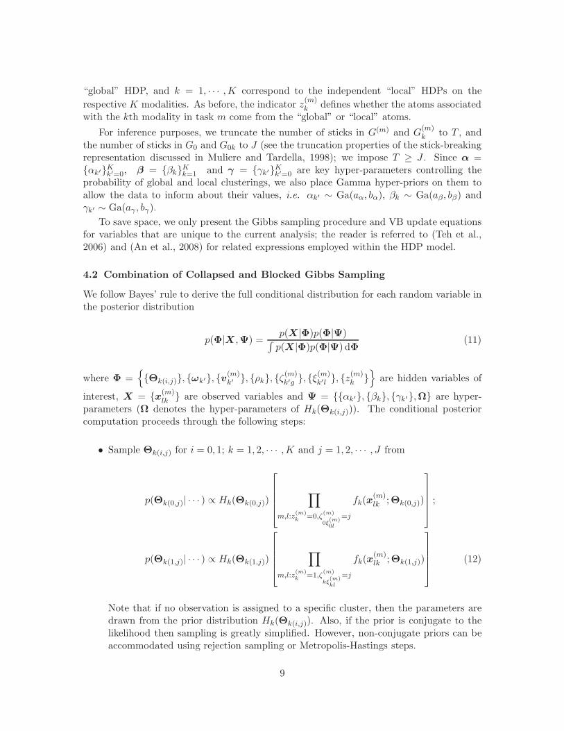
• Sample Θk(i,j) for i = 0, 1; k = 1, 2, · · · ,K and j = 1, 2, · · · , J from
p(Θk(0,j)| · · · ) ∝ Hk(Θk(0,j))
∏
m,l:z(m)k
=0,ζ(m)
0ξ(m)0l
=j
fk(x(m)lk ;Θk(0,j))
;
p(Θk(1,j)| · · · ) ∝ Hk(Θk(1,j))
∏
m,l:z(m)k
=1,ζ(m)
kξ(m)kl
=j
fk(x(m)lk ;Θk(1,j))
(12)
Note that if no observation is assigned to a specific cluster, then the parameters aredrawn from the prior distribution Hk(Θk(i,j)). Also, if the prior is conjugate to thelikelihood then sampling is greatly simplified. However, non-conjugate priors can beaccommodated using rejection sampling or Metropolis-Hastings steps.
9

• Sample ωk′j for k′ = 0, 1, · · · ,K and j = 1, 2, · · · , J by generating
p(ω′k′j | · · · ) ∝
Beta(
1 +∑M
m=1
∑Tg=1 1(ζ
(m)k′g = j), γk′ +
∑Mm=1
∑Tg=1
∑Jh:h>j 1
(
ζ(m)k′g = h
))
;
j = 1, 2, · · · , J − 1;
ω′k′J = 1 (13)
and constructing ωk′j = ω′k′j
∏j−1h=1(1 − ω′
k′h).
• Sample v(m)k′g for k′ = 0, 1, · · · ,K; g = 1, 2, · · · , T and m = 1, 2, · · · ,M by generating
p(v′(m)k′g | · · · ) ∝ Beta
1 +
Lm∑
l=1
1(ξ(m)k′l = g), αk′ +
Lm∑
l=1
T∑
h:h>g
1(ξ(m)k′l = h)
;
g = 1, 2, · · · , T − 1;
v′(m)k′T = 1 (14)
and constructing v(m)k′g = v
′(m)k′g
∏g−1h=1(1 − v
′(m)k′h ).
• Sample ρk for k = 1, 2, · · · ,K from
p(ρk| · · · ) ∝ Beta
(
1 +M∑
m=1
1(z(m)k = 0), βk +
M∑
m=1
1(z(m)k = 1)
)
(15)
• Sample ζ(m)k′g for k′ = 0, 1, · · · ,K; g = 1, 2, · · · , T and m = 1, 2, · · · ,M from a multi-
nomial distribution with probabilities
p(ζ(m)0g = j| · · · ) ∝ p(ζ
(m)0g = j|ζ
(m)0g′ g′ 6=g, γ0)
∏
k:z(m)k
=0,l:ξ(m)0l
=gfk(x
(m)lk ;Θk(0,j))
=
(
1+∑
g′ 6=g 1(ζ(m)
0g′=j)
1+γ0+∑
g′ 6=g 1(ζ(m)
0g′≥j)
∏
h<j
γ0+∑
g′ 6=g 1(ζ(m)
0g′>h)
1+γ+∑
g′ 6=g 1(ζ(m)
0g′≥h)
)
∏
k:z(m)k
=0,l:ξ(m)0l
=gfk(x
(m)lk ;Θk(0,j))
;
p(ζ(m)kg = j| · · · ) ∝ p(ζ
(m)kg = j|ζ
(m)kg′ g′ 6=g, γk)1(z
(m)k = 1)
∏
l:ξ(m)kl
=gfk(x
(m)lk ;Θk(1,j))
=
(
1+∑
g′ 6=g 1(ζ(m)
kg′=j)
1+γk+∑
g′ 6=g 1(ζ(m)
kg′≥j)
∏
h<j
γk+∑
g′ 6=g 1(ζ(m)
kg′>h)
1+γk+∑
g′ 6=g 1(ζ(m)
kg′≥h)
)
1(z(m)k = 1)
∏
l:ξ(m)kl
=gfk(x
(m)lk ;Θk(1,j))
(16)
10
• Sample ξ(m)k′l for k′ = 0, 1, · · · ,K; l = 1, 2, · · · , Lm and m = 1, 2, · · · ,M from a
multinomial distribution with probabilities
p(ξ(m)0l = g| · · · ) ∝ p(ξ
(m)0l = g|ξ
(m)0l′ l′ 6=l, α0)
∏
k:z(m)k
=0fk(x
(m)lk ;Θ
k(0,ζ(m)0g )
)
=
(
1+∑
l′ 6=l 1(ξ(m)
0l′=g)
1+α0+∑
l′ 6=l 1(ξ(m)
0l′≥g)
∏
h<g
α0+∑
l′ 6=l 1(ξ(m)
0l′>h)
1+α0+∑
l′ 6=l 1(ξ(m)
0l′≥h)
)
∏
k:z(m)k
=0fk(x
(m)lk ;Θ
k(0,ζ(m)0g )
)
;
p(ξ(m)kl = g| · · · ) ∝ p(ξ
(m)kl = g|ξ
(m)kl′ l′ 6=l, αk)1(z
(m)k = 1)fk(x
(m)lk ;Θ
k(1,ζ(m)kg
))
=
(
1+∑
l′ 6=l 1(ξ(m)
kl′=g)
1+αk+∑
l′ 6=l 1(ξ(m)
kl′≥g)
∏
h<g
αk+∑
l′ 6=l 1(ξ(m)
kl′>h)
1+αk+∑
l′ 6=l 1(ξ(m)
kl′≥h)
)
1(z(m)k = 1)fk(x
(m)lk ;Θ
k(1,ζ(m)kg
))
(17)
• Sample z(m)k for k = 1, 2, · · · ,K, and m = 1, 2, · · · ,M from a Bernoulli distribution
with probabilities
p(z(m)k = 0| · · · ) ∝ p(z
(m)k = 0|z
(m)k′′ k′′ 6=k, βk)
∏Lm
l=1 fk(x(m)lk ; Θ
k(0,ζ(m)
0ξ(m)0l
))
=1+∑
k′′ 6=k 1(z(m)
k′′=0)
1+βk+∑
k′′ 6=k 1(z(m)
k′′≥0)
∏Lm
l=1 fk(x(m)lk ;Θ
k(0,ζ(m)
0ξ(m)0l
))
;
p(z(m)k = 1| · · · ) ∝ p(z
(m)k = 1|z
(m)k′′ k′′ 6=k, βk)
∏Lm
l=1 fk(x(m)lk ; Θ
k(1,ζ(m)
kξ(m)kl
))
=
(
1+∑
k′′ 6=k 1(z(m)
k′′=1)
1+βk+∑
k′′ 6=k 1(z(m)
k′′≥1)
βk+∑
k′′ 6=k 1(z(m)
k′′>0)
1+βk+∑
k′′ 6=k 1(z(m)
k′′≥0)
)
∏Lm
l=1 fk(x(m)lk ;Θ
k(1,ζ(m)
kξ(m)kl
))
(18)
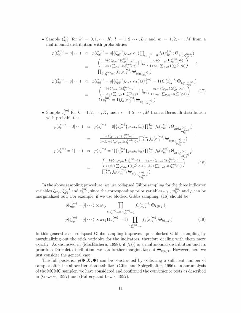
In the above sampling procedure, we use collapsed Gibbs sampling for the three indicator
variables ζk′g, ξ(m)k′l and z
(m)k , since the corresponding prior variables ωk′ , v
(m)k′ and ρ can be
marginalized out. For example, if we use blocked Gibbs sampling, (16) should be
p(ζ(m)0g = j| · · · ) ∝ ω0j
∏
k:z(m)k
=0,l:ξ(m)0l
=g
fk(x(m)lk ;Θk(0,j));
p(ζ(m)kg = j| · · · ) ∝ ωkj1(z
(m)k = 1)
∏
l:ξ(m)kl
=g
fk(x(m)lk ;Θk(1,j)) (19)
In this general case, collapsed Gibbs sampling improves upon blocked Gibbs sampling bymarginalizing out the stick variables for the indicators, therefore dealing with them moreexactly. As discussed in (MacEachern, 1998), if fk(·) is a multinomial distribution and itsprior is a Dirichlet distribution, we can further marginalize out Θk(i,j). However, here wejust consider the general case.
The full posterior p(Φ|X,Ψ) can be constructed by collecting a sufficient number ofsamples after the above iteration stabilizes (Gilks and Spiegelhalter, 1996). In our analysisof the MCMC sampler, we have considered and confirmed the convergence tests as describedin (Geweke, 1992) and (Raftery and Lewis, 1992).
11
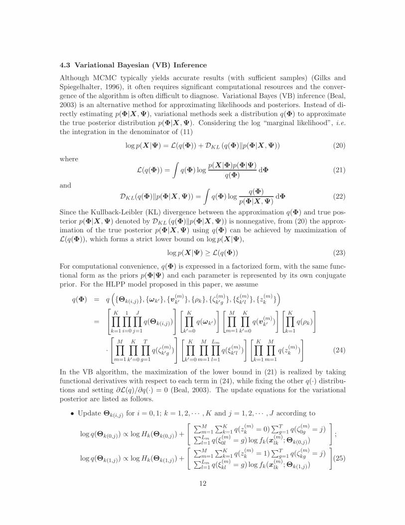
4.3 Variational Bayesian (VB) Inference
Although MCMC typically yields accurate results (with sufficient samples) (Gilks andSpiegelhalter, 1996), it often requires significant computational resources and the conver-gence of the algorithm is often difficult to diagnose. Variational Bayes (VB) inference (Beal,2003) is an alternative method for approximating likelihoods and posteriors. Instead of di-rectly estimating p(Φ|X,Ψ), variational methods seek a distribution q(Φ) to approximatethe true posterior distribution p(Φ|X ,Ψ). Considering the log “marginal likelihood”, i.e.the integration in the denominator of (11)
log p(X |Ψ) = L(q(Φ)) + DKL (q(Φ)‖p(Φ|X ,Ψ)) (20)
where
L(q(Φ)) =
∫
q(Φ) logp(X |Φ)p(Φ|Ψ)
q(Φ)dΦ (21)
and
DKL(q(Φ)‖p(Φ|X ,Ψ)) =
∫
q(Φ) logq(Φ)
p(Φ|X,Ψ)dΦ (22)
Since the Kullback-Leibler (KL) divergence between the approximation q(Φ) and true pos-terior p(Φ|X,Ψ) denoted by DKL (q(Φ)‖p(Φ|X ,Ψ)) is nonnegative, from (20) the approx-imation of the true posterior p(Φ|X,Ψ) using q(Φ) can be achieved by maximization ofL(q(Φ)), which forms a strict lower bound on log p(X|Ψ),
log p(X|Ψ) ≥ L(q(Φ)) (23)
For computational convenience, q(Φ) is expressed in a factorized form, with the same func-tional form as the priors p(Φ|Ψ) and each parameter is represented by its own conjugateprior. For the HLPP model proposed in this paper, we assume
q(Φ) = q(
Θk(i,j), ωk′, v(m)k′ , ρk, ζ
(m)k′g , ξ
(m)k′l , z
(m)k
)
=
K∏
k=1
1∏
i=0
J∏
j=1
q(Θk(i,j))
[
K∏
k′=0
q(ωk′)
] [
M∏
m=1
K∏
k′=0
q(v(m)k′ )
] [
K∏
k=1
q(ρk)
]
·
M∏
m=1
K∏
k′=0
T∏
g=1
q(ζ(m)k′g )
[
K∏
k′=0
M∏
m=1
Lm∏
l=1
q(ξ(m)k′l )
] [
K∏
k=1
M∏
m=1
q(z(m)k )
]
(24)
In the VB algorithm, the maximization of the lower bound in (21) is realized by takingfunctional derivatives with respect to each term in (24), while fixing the other q(·) distribu-tions and setting ∂L(q)/∂q(·) = 0 (Beal, 2003). The update equations for the variationalposterior are listed as follows.
• Update Θk(i,j) for i = 0, 1; k = 1, 2, · · · ,K and j = 1, 2, · · · , J according to
log q(Θk(0,j)) ∝ logHk(Θk(0,j)) +
[
∑Mm=1
∑Kk=1 q(z
(m)k = 0)
∑Tg=1 q(ζ
(m)0g = j)
∑Lm
l=1 q(ξ(m)0l = g) log fk(x
(m)lk ;Θk(0,j))
]
;
log q(Θk(1,j)) ∝ logHk(Θk(1,j)) +
[
∑Mm=1
∑Kk=1 q(z
(m)k = 1)
∑Tg=1 q(ζ
(m)kg = j)
∑Lm
l=1 q(ξ(m)kl = g) log fk(x
(m)lk ;Θk(1,j))
]
(25)
12

If the prior is conjugate to the likelihood then we can easily get the update equations.
• Update ω′k′j for k′ = 0, 1, · · · ,K and j = 1, 2, · · · , J − 1 according to
q(ω′k′j) = Beta(ω′
k′j; γ(1)k′j , γ
(2)k′j)
γ(1)k′j = 1 +
∑Mm=1
∑Tg=1 q(ζ
(m)k′g = j), γ
(2)k′j = γk′ +
∑Mm=1
∑Tg=1
∑Jh:h>j q(ζ
(m)k′g = h)(26)
Since ωk′j = ω′k′j
∏j−1h=1(1 − ω′
k′h), updating of ω′k′ is equivalent to updating the pos-
terior of ωk′ .
• Update v(m)k′g for k′ = 0, 1, · · · ,K; g = 1, 2, · · · , T and m = 1, 2, · · · ,M according to
q(v′(m)k′g ) = Beta(v
′(m)k′g ; α
(m,1)k′g , α
(m,2)k′g );
α(m,1)k′g = 1 +
∑Lm
l=1 q(ξ(m)k′l = g), α
(m,2)k′g = αk′ +
∑Lm
l=1
∑Th:h>g q(ξ
(m)k′l = h) (27)
Since v(m)k′g = v
′(m)k′g
∏g−1h=1(1 − v
′(m)k′h ), updating of v
′(m)k′ is equivalent to updating the
posterior of v(m)k′ .
• Update ρk for k = 1, 2, · · · ,K according to
q(ρk) = Beta(ρk; βk1, βk2);
βk1 = 1 +∑M
m=1 q(z(m)k = 0), βk2 = βk +
∑Mm=1 q(z
(m)k = 1) (28)
• Update ζ(m)k′g for k′ = 0, 1, · · · ,K; g = 1, 2, · · · , T and m = 1, 2, · · · ,M according to a
multinomial distribution with probabilities
q(ζ(m)0g = j) ∝ exp
(
∑j−1h=1[ψ(γ
(2)0h ) − ψ(γ
(1)0h + γ
(2)0h )] + [ψ(γ
(1)0j ) − ψ(γ
(1)0j + γ
(2)0j )]
+∑K
k=1 q(z(m)k = 0)
∑Lm
l=1 q(ξ(m)kl = g) log fk(x
(m)lk ;Θk(0,j))
)
;
q(ζ(m)kg = j) ∝ exp
(
∑j−1h=1[ψ(γ
(2)kh ) − ψ(γ
(1)kh + γ
(2)kh )] + [ψ(γ
(1)kj ) − ψ(γ
(1)kj + γ
(2)kj )]
+∑K
k=1 q(z(m)k = 1)
∑Lm
l=1 q(ξ(m)kl = g) log fk(x
(m)lk ;Θk(1,j))
)
(29)
where ψ(A) = ∂∂A
log Γ(A) and Γ(·) represents the Gamma function.
• Update ξ(m)k′l for k′ = 0, 1, · · · ,K; l = 1, 2, · · · , Lm and m = 1, 2, · · · ,M according to
a multinomial distribution with probabilities
q(ξ(m)0l = g) ∝ exp
∑g−1h=1[ψ(α
(m,2)0h ) − ψ(α
(m,1)0h + α
(m,2)0h )]
+[ψ(α(m,1)0g ) − ψ(α
(m,1)0g + α
(m,2)0g )]
+∑K
k=1 q(z(m)k = 0)
∑Jj=1 q(ζ
(m)0g = j) log fk(x
(m)lk ;Θk(0,j))
;
q(ξ(m)kl = g) ∝ exp
∑g−1h=1[ψ(α
(m,2)kh ) − ψ(α
(m,1)kh + α
(m,2)kh )]
+[ψ(α(m,1)kg ) − ψ(α
(m,1)kg + α
(m,2)kg )]
+∑K
k=1 q(z(m)k = 1)
∑Jj=1 q(ζ
(m)kg = j) log fk(x
(m)lk ;Θk(1,j))
(30)
13
• Update z(m)k for k = 1, 2, · · · ,K, and m = 1, 2, · · · ,M according to a Bernoulli
distribution with probabilities
q(z(m)k = 0) ∝ exp
(
[ψ(βk1) − ψ(βk1 + βk2)] +∑Lm
l=1
∑Tg=1
∑Jj=1 q(ζ
(m)0g = j)q(ξ
(m)0l = g) log fk(x
(m)lk ;Θk(0,j))
)
;
q(z(m)k = 1) ∝ exp
(
[ψ(βk2) − ψ(βk1 + βk2)] +∑Lm
l=1
∑Tg=1
∑Jj=1 q(ζ
(m)kg = j)q(ξ
(m)kl = g) log fk(x
(m)lk ;Θk(1,j))
)
(31)
The local maximum of the lower bound L(q) is achieved by iteratively updating theparameters of the variational distributions q(·) according to the above equations. Eachiteration guarantees to either increase the lower bound or leave it unchanged. We terminatethe algorithm when the change in L(q) is negligibly small. L(q) can be computed bysubstituting the updated q(·) and the prior distributions p(Φ|Ψ) into (21). To mitigatesensitivity of VB to initialization considerations and local-optimal solutions, we typicallyrun the VB algorithm multiple times with different initializations, and select the result withthe maximum lower bound.
In the analysis considered here we perform VB inference on the original model, sincethis was relatively efficient computationally. One may alternatively perform VB inferenceon the collapsed model (MacEachern, 1998; Teh et al., 2007), as applied to the combinationof collapsed and blocked Gibbs sampling discussed in detail above.
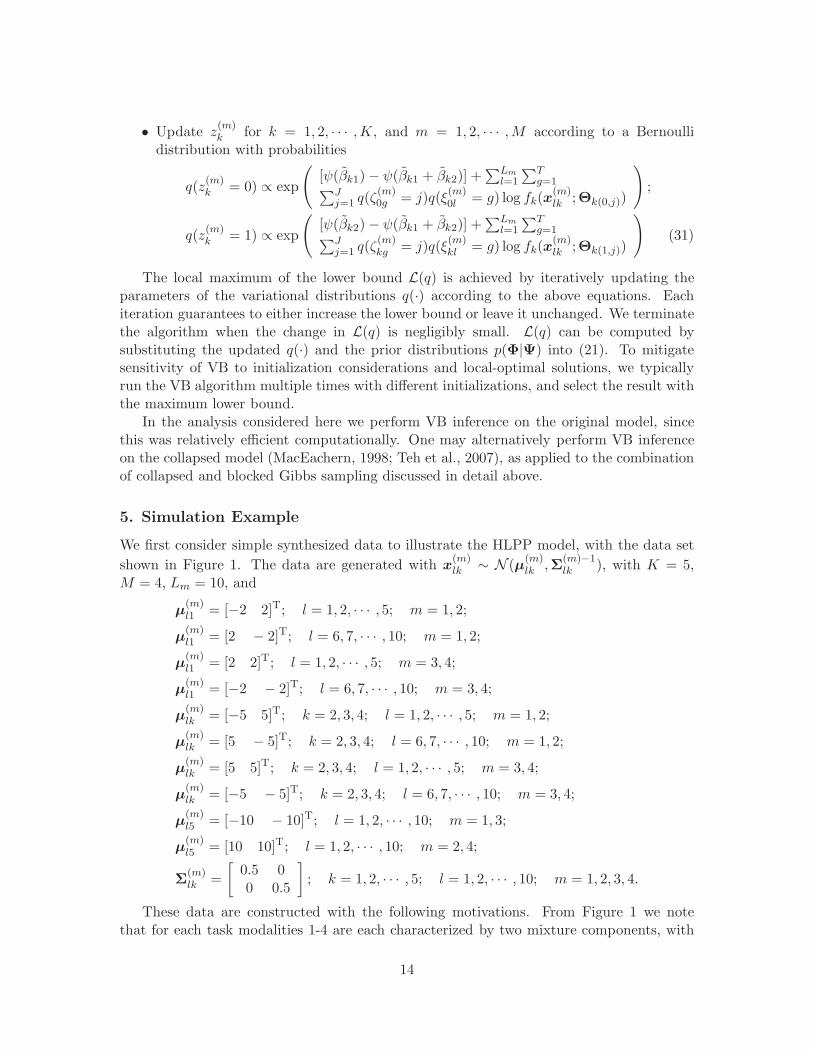
5. Simulation Example
We first consider simple synthesized data to illustrate the HLPP model, with the data set
shown in Figure 1. The data are generated with x(m)lk ∼ N (µ
(m)lk ,Σ
(m)−1lk ), with K = 5,
M = 4, Lm = 10, and
µ(m)l1 = [−2 2]T; l = 1, 2, · · · , 5; m = 1, 2;
µ(m)l1 = [2 − 2]T; l = 6, 7, · · · , 10; m = 1, 2;
µ(m)l1 = [2 2]T; l = 1, 2, · · · , 5; m = 3, 4;
µ(m)l1 = [−2 − 2]T; l = 6, 7, · · · , 10; m = 3, 4;
µ(m)lk = [−5 5]T; k = 2, 3, 4; l = 1, 2, · · · , 5; m = 1, 2;
µ(m)lk = [5 − 5]T; k = 2, 3, 4; l = 6, 7, · · · , 10; m = 1, 2;
µ(m)lk = [5 5]T; k = 2, 3, 4; l = 1, 2, · · · , 5; m = 3, 4;
µ(m)lk = [−5 − 5]T; k = 2, 3, 4; l = 6, 7, · · · , 10; m = 3, 4;
µ(m)l5 = [−10 − 10]T; l = 1, 2, · · · , 10; m = 1, 3;
µ(m)l5 = [10 10]T; l = 1, 2, · · · , 10; m = 2, 4;
Σ(m)lk =
[
0.5 00 0.5
]
; k = 1, 2, · · · , 5; l = 1, 2, · · · , 10; m = 1, 2, 3, 4.
These data are constructed with the following motivations. From Figure 1 we notethat for each task modalities 1-4 are each characterized by two mixture components, with
14

modality 5 characterized by a single task-dependent cluster. Note also that modalities 1-4 have the same mixture construction in tasks 1 and 2, as well as (separately) the samemixture construction in tasks 3 and 4. The task-dependent properties of modality 5 aredistinct from those of modalities 1-4. Therefore, we anticipate that modalities 1-4 willexhibit “global” clustering, with tasks 1 and 2 clustered together, and similarly tasks 3and 4 clustered together. By contrast, modality 5 is expected to exhibit distinct “local”clustering, with tasks 1 and 3 clustered together, and tasks 2 and 4 clustered together.Global clustering across all five modalities is clearly inappropriate. However, one may inprinciple cluster the data independently across tasks for each of the five modalities; thishas motivated the construction of the data in modality 1. Note that the differences in themixture components for modality 1 are far more subtle than those associated with modalities2-4. Below we demonstrate that when an independent HDP prior is used for task-dependentclustering for each of the modalities, the subtleties associated with modality 1 are missed.By contrast, the HLPP captures the clear clusterings associated with modalities 2-4, andin so doing “pulls along” the same task clustering for modality 1, thereby improving themixture model for modality 1. The HLPP also allows idiosyncratic “local” clustering formodality 5.
−10 0 10
−100
10
Task 1
Mod
ality
1x 2
−10 0 10
−100
10
Task 2
−10 0 10
−100
10
Task 3
−10 0 10
−100
10
Task 4
−10 0 10
−100
10
Mod
ality
2x 2
−10 0 10
−100
10
−10 0 10
−100
10
−10 0 10
−100
10
−10 0 10
−100
10
Mod
ality
3x 2
−10 0 10
−100
10
−10 0 10
−100
10
−10 0 10
−100
10
−10 0 10
−100
10
Mod
ality
4x 2
−10 0 10
−100
10
−10 0 10
−100
10
−10 0 10
−100
10
−10 0 10
−100
10
x1
Mod
ality
5x 2
−10 0 10
−100
10
x1
−10 0 10
−100
10
x1
−10 0 10
−100
10
x1
Figure 1: Synthetic data, where x1 and x2 represent components of the vector x.
The HLPP model is implemented for this synthetic data set, with J = 50 and T = 50.The base distribution is specified as Hk =
∏2n=1[N (µkn; r0n, t0Σkn) − Ga(Σkn; d0, s0n)] for
k = 1, 2, · · · , 5, with r0n = 0, t0 = 0.01, d0 = 4, and s0n = 1. We place Gamma priorsGa(10−6, 10−6) on α and γ, Ga(10−6, 1) on β. These parameters were not tuned, and manydifferent settings yield comparable results. The MCMC algorithm described in Section 4.2is used to obtain samples of posteriors under the HLPP. The results shown below are basedon 10,000 collection samples obtained after a burn-in period of 5,000 iterations. Rapid
15

Data Index
DataIndex
Modality 1
10 20 30 40
10
20
30
40
Data Index
Modality 2~4
10 20 30 40Data Index
Modality 5
10 20 30 400
0.2
0.4
0.6
0.8
1Task1
Task2
Task3
Task4
(a)
Data Index
Modality 2~4
10 20 30 40
Data Index
Modality 5
10 20 30 400
0.2
0.4
0.6
0.8
1Task1
Task2
Task3
Task4
Data Index
DataIndex
Modality 1
10 20 30 40
10
20
30
40
(b)
Data Index
DataIndex
10 20 30 40
10
20
30
40 0
0.2
0.4
0.6
0.8
1Task1
Task2
Task3
Task4
(c)
Figure 2: Pairwise posterior probabilities of two data samples being assigned to the samecluster for the simulation example analyzed using the HLPP, independent HDPand HDP models. (a) HLPP results; (b) independent HDP results; (c) “global”HDP results.
16

1~5 6~10 11~15 16~20 21~25 26~30 31~35 36~40−10
0
10
Modality 1x 1 V
alue
Data Index
1~5 6~10 11~15 16~20 21~25 26~30 31~35 36~40−10
0
10
Modality 2~4
x 1 Val
ue
Data Index
1~5 6~10 11~15 16~20 21~25 26~30 31~35 36~40−10
0
10
Modality 5
x 1 Val
ue
Data Index
(a)
1~5 6~10 11~15 16~20 21~25 26~30 31~35 36~40−10
0
10
Modality 1
x 2 Val
ue
Data Index
1~5 6~10 11~15 16~20 21~25 26~30 31~35 36~40−10
0
10
Modality 2~4
x 2 Val
ue
Data Index
1~5 6~10 11~15 16~20 21~25 26~30 31~35 36~40−10
0
10
Modality 5
x 2 Val
ue
Data Index
(b)
Figure 3: Posterior means and 95% credible intervals for the mean parameters of eachmodality in the simulation example. The red solid bar indicates the estimatesfor the HLPP model, the blue shows those for the independent HDP model, thegreen shows those for the HDP model, and the dark shows the true values of themean parameters. (a) the first dimension of the data; (b) the second dimensionof the data.
17

convergence has been observed in the diagnostic tests described in (Geweke, 1992) and(Raftery and Lewis, 1992).
From the indicators z(m)k 5,4
k=1,m=1 in the HLPP model, we observed that tasks 1-4selected global clustering and task 5 selected local clustering. Since the two clusters inmodality 1 are subtle, the good clustering performance of modalities 2-4 helps modality 1obtain the correct clustering, as indicated above. Figure 2(a) plots the posterior probabilityof two data samples being assigned to the same cluster separately for each of the fivemodalities, as inferred via the HLPP model. It is apparent that the true clustering structureis well represented by the HLPP model. For comparison, Figures 2(b) and 2(c) present thecorresponding results obtained by the independent HDP model (special case with βk → ∞)and global HDP model (special case with βk → 0), respectively. The similarity matrix ofthe independent HDP model is not correct for modality 1, impacting model performance asdiscussed further below. Because of the idiosyncratic clustering structure of modality 5, thesimilarity matrix of the HDP model is very poor. Figure 3 shows the inferred data-specific
posterior means and 95% credible intervals for the mean parameters µ(m)lk 10,5,4
l=1,k=1,m=1 viathe HLPP model (red), along with the results for the independent HDP model (blue) andthe HDP model (green). The black lines represent the true values of the mean parameters.It is clear the posterior densities via the HLPP model are concentrated around the truevalues, while there are mistakes for modality 1 via the independent HDP model and formodality 5 via the HDP model. In addition, the 95% credible intervals from the HLPPanalysis are the tightest, compared with the independent HDP and HDP analysis; this isattributed to proper global and local sharing explicitly imposed by HLPP.
6. Gene-Expression Analysis Application
To further illustrate the proposed HLPP model, we consider an application to gene-expressiondata, here for a Dengue virus study (Fink et al., 2007). The HLPP is applied to sparse factoranalysis (Carvalho et al.; Pournara and Wernish, 2007; Fokoue, 2004; Knowles and Ghahra-mani, 2007), where the latent factors correspond to the “modalities”. The factor scoresrepresent the data, although now these data are latent. For the Dengue gene-expressiondata under study we have expression values at multiple time points after cell exposure withthe virus, and each of the times represents a task; for each task (time) we have multiplegene-expression samples (from cells exposed to either live or heat inactivated virus). Wewish to impose the belief that the factor scores, which can be interpreted as meta-geneexpression levels underlying many genes in a pathway, cluster across tasks (time). How-ever, as different meta-genes are involved in different biologic pathways and have varyingrelationships with viral exposure, the factor scores may vary in their temporal clusteringstructure. Therefore, we do not expect all components of the factor scores to cluster inthe same way. This anticipated phenomenon mitigates the use of global HDP clustering(i.e., the same clustering across all factor scores). However, if we cluster the individualcomponents of the factor scores independently, we do not account for anticipated statisticalcorrelation. This therefore motivates the HLPP construction.
18

6.1 Sparse Factor Analysis for Gene Expression Data
Assume y(m)l is an N × 1 vector representing the gene expressions for N genes, for cell
l at time m, with m = 1, 2, · · · ,M and l = 1, 2, · · · , Lm. It is assumed that Y =
[y(1)1 · · ·y
(1)L1
· · · y(M)1 · · ·y
(M)LM
] is already normalized to zero mean in each row. We con-
sider the case N ≫ K =∑M
m=1 Lm, which is typical. The parametric sparse factor analysismodel (Pournara and Wernish, 2007) characterizes dependence in the high-dimensional genexpression measurements using
y(m)l = Bλ
(m)l + ǫ
(m)l ; l = 1, 2, · · · , Lm; m = 1, 2, · · · ,M
λ(m)l ∼ N (0, I); l = 1, 2, · · · , Lm; m = 1, 2, · · · ,M
Bnk ∼ N (0, η−1nk )); n = 1, 2, · · · , N ; k = 1, 2, · · · ,K
ηnk ∼ Ga(a0, b0); n = 1, 2, · · · , N ; k = 1, 2, · · · ,K
ǫ(m)nl ∼ N (0, ϕ−1
n )); l = 1, 2, · · · , Lm; m = 1, 2, · · · ,M ; n = 1, 2, · · · , N
ϕn ∼ Ga(g0, h0); n = 1, 2, · · · , N (32)
where Bnk is the (n, k)-component of the factor-loading matrix B, and λ(m)l represents the
factor score associated with cell l at time m. Typically one sets K, with K ≪ N . Note thatthe components of B are drawn independently from a Student-t distribution, and hencewith appropriate choice of a0 and b0 the matrix B is sparse. Alternatively, one may use a“spike-slab” sparseness construction, as in (Carvalho et al.); (Pournara and Wernish, 2007)gives a comprehensive review of different sparseness priors used for sparse factor analysis.
Both B and all λ(m)l are inferred by the model simultaneously. As discussed in (Carvalho
et al.), since B is “sparse”, which means many of the elements of B are close to zero, eachcolumn ideally will represent a particular biological “pathway”, composed of a relativelysmall number of relevant genes related to a given latent factor, which correspond to thosehaving factor loadings not close to zero. This is discussed further when presenting resultsfor the time-evolving Dengue virus data (Fink et al., 2007).
6.2 The Extended Factor Model with the HLPP Prior
In the HLPP factor analysis (HLPP-FA) model, the construction of B and ǫ(m)l is unchanged
from above, and therefore for simplicity it is not repeated below. What is different is the
manner in which the factor scores λ(m)l are drawn from the prior. Specifically, we have
λ(m)lk ∼ N (µ
(m)lk ,Σ
(m)−1lk ), (µ
(m)lk ,Σ
(m)lk ) ∼ LPP(β, G(m), G
(m)k K
k=1)
l = 1, 2, · · · , Lm; k = 1, 2, · · · ,K; m = 1, 2, · · · ,M
G(m)k ∼ HDP(αk, γk,Hk); k = 1, 2, · · · ,K; m = 1, 2, · · · ,M
G(m) ∼ HDP(α0, γ0,
K∏
k=1
Hk); m = 1, 2, · · · ,M
Hk = N − Ga(r0, t0, d0, s0); k = 1, 2, · · · ,K (33)
where here (µlk,Σlk) = θlk. Note that (32) assumes that the latent factors are normallydistributed and have the same distribution at the different times. In contrast, (33) charac-
19

terizes the distribution of the latent factors using a flexible mixture of normals, which canvary over time, while borrowing information. This borrowing is accomplished by incorpo-rating the same mean and variance in the normal mixture components at the different timesthrough the HDP structure, while also flexibly clustering latent factors over time throughfavoring allocation to the same mixture component. However, the LPP structure does notforce a latent factor to be allocated to the same component at all times, but allows occa-sional local switching of components. This is important in flexibly characterizing changesthat can occur as a result of the virus.
In the following examples, we also put Gamma priors on α, β and γ. The model in(33) is a direct combination of (5) and (32), and therefore the MCMC inference can alsobe directly derived based on Section 4.2 and (Fokoue, 2004). Here we only give the main
modification concerning sampling latent variable λ(m)lk .
• Let y(m)∗lk = yl −
∑
k′′ 6=k Bk′′λ(m)lk′′ for k = 1, 2, · · · ,K; l = 1, 2, · · · , Lm and m =
1, 2, · · · ,M . Since y(m)∗lk ∼ N (Bkλ
(m)lk ,diag−1(ϕ)) , we can sample λ
(m)kl from
p(λ(m)lk | · · · ) ∝ N
(BTk diag(ϕ)Bk + Σ∗−1
k(0,ζ(m)
0ξ(m)0l
))−1
(BTk diag(ϕ)y
(m)∗lk + Σ∗
k(0,ζ(m)
0ξ(m)0l
)) µ∗
k(0,ζ(m)
0ξ(m)0l
),
(BTk diag(ϕ)Bk + Σ∗−1
k(0,ζ(m)
0ξ(m)0l
))−1
if z(m)k = 0
p(λ(m)lk | · · · ) ∝ N
(BTk diag(ϕ)Bk + Σ∗−1
k(1,ζ(m)
kξ(m)kl
))−1
(BTk diag(ϕ)y
(m)∗lk + Σ∗
k(1,ζ(m)
kξ(m)kl
)) µ∗
k(1,ζ(m)
kξ(m)kl
),
(BTk diag(ϕ)Bk + Σ∗−1
k(1,ζ(m)
kξ(m)kl
))−1
if z(m)k = 1
(34)
The symbols correspond to those used in (10), where(µ∗k(i,j),Σ
∗k(i,j)) = Θk(i,j). The remain-
ing variables specified in (33) are sampled in a similar manner as in Section 4.2 and (Fokoue,2004).
6.3 Experimental Results for Gene-Expression Data
The Dengue data considered here is time-evolving expression data, and is publicly availableat http://www.ncbi.nlm.nih.gov/projects/geo (accession number is GSE6048). The dataconsist of six groups (tasks) of samples measured at six time points. The six time pointsare 3, 6, 12, 24, 48 and 72 hours after a HepG2 cell is exposed to the NGC Dengue virus (bothlive and heat-inactivated/dead viruses are used). At each time point the transcriptome isprofiled using biological repeats. The corresponding number of samples at the six timepoints are 10, 12, 12, 12, 12, 11. The number of genes in this dataset is 20,160. Thedetailed description of these genes can be found in (Fink et al., 2007). In the plots thatfollow, the samples are ordered according to their time points, from early to late time. Onequestion of interest is whether cells with live virus have a systematically different profile
20

0 50
−100
1020
Factor 1
Fac
tor
Sco
re
0 50−20−10
010
Factor 2
0 50−20
020
Factor 3
0 50
02040
Factor 4
0 50
−100
1020
Factor 5
0 50−30−20−10
010
Factor 6
Fac
tor
Sco
re
0 50−20
020
Factor 7
0 50−20
020
Factor 8
0 50−10
010
Factor 9
0 50−20
020
Factor 10
0 50
−200
20
Factor 11
Fac
tor
Sco
re
0 50
−100
1020
Factor 12
0 50
−100
10
Factor 13
0 50−20
020
Factor 14
0 50
0102030
Factor 15
0 50−10
010
Factor 16
Fac
tor
Sco
re
0 50−30−20−10
010
Factor 17
0 50−20
02040
Factor 18
0 50−20−10
010
Factor 19
0 50−10
01020
Factor 20
0 50
−100
10Factor 21
Fac
tor
Sco
re
0 50
−200
20Factor 22
0 50−20
020
Factor 23
0 50−10
01020
Factor 24
0 50−10
01020
Factor 25
0 50−10
010
Factor 26
Data Index
Fac
tor
Sco
re
0 50
−200
20Factor 27
Data Index0 50
−100
1020
Factor 28
Data Index0 50
−200
20Factor 29
Data Index0 50
02040
Factor 30
Data Index
Figure 4: Posterior means for the components of each factor score, as computed via thesparse factor analysis model in (Carvalho et al.). Different color denote differenttime points (tasks), time increases from left to right across the horizontal axis;“.” represents the cell cultures exposed to live virus, and “x” represents the cellcultures exposed to heat inactivated virus.
21

0 50−10
010
Factor 1F
acto
r S
core
0 50
−505
10Factor 2
0 50−5
05
Factor 3
0 50−10
−505
Factor 4
0 50−10
01020
Factor 5
0 50−5
05
10Factor 6
Fac
tor
Sco
re
0 50−10
010
Factor 7
0 50−5
05
10
Factor 8
0 50
−505
Factor 9
0 50−10
010
Factor 10
0 50−5
0
5Factor 11
Fac
tor
Sco
re
0 50−5
05
10Factor 12
0 50
−100
10
Factor 13
0 50−5
05
Factor 14
0 50−10
−505
Factor 15
0 50−5
05
Factor 16
Fac
tor
Sco
re
0 50
−100
10
Factor 17
0 50−10
0
10Factor 18
0 50
−505
Factor 19
0 50−5
05
10Factor 20
0 50
01020
Factor 21
Fac
tor
Sco
re
0 50−20−10
010
Factor 22
0 50−10
010
Factor 23
0 50−4−2
024
Factor 24
0 50
05
10Factor 25
0 50
−505
Factor 26
Data Index
Fac
tor
Sco
re
0 50−5
05
1015
Factor 27
Data Index0 50
−15−10
−505
Factor 28
Data Index0 50
−100
10
Factor 29
Data Index0 50
−505
10
Factor 30
Data Index
Figure 5: Posterior means for the components of each factor score, as computed via thesparse factor analysis model with the HLPP prior, where different color denotedifferent time points (tasks), time increases from left to right across the horizontalaxis; “.” represents the cell cultures exposed to live virus, and “x” represents thecell cultures exposed to heat inactivated virus.
Task Index
Fac
tor
Inde
x
3hr 6hr 12hr 24hr 48hr 72hr
5
10
15
20
25
30 0:Global
1:Local
Figure 6: The average indicator matrix for selecting global or local clustering via the sparsefactor analysis model with the HLPP prior.
22

of changes in the latent factor score distributions over time relative to cells with deadvirus. For factors exhibiting such changes, it is also of interest to identify the associatedgenes (i.e., those having loadings not close to zero) and assess whether they have knownbiological significance. In (Fink et al., 2007), differential gene expression was noted betweencells exposed to live or heat inactivated virus at 48 hours post exposure onset.
Factor 1~4, 6~20, 24~30
Data Index
DataIndex
20 40 60
10
20
30
40
50
60
3hr
6hr
12hr
24hr
48hr
72hr
Factor 5
Data Index20 40 60
Factor 21
Data Index20 40 60
0
0.2
0.4
0.6
0.8
1
3hr
6hr
12hr
24hr
48hr
72hr
Factor 22
Data Index
DataIndex
20 40 60
10
20
30
40
50
60
Factor 23
Data Index20 40 60
0
0.2
0.4
0.6
0.8
1
Figure 7: Pairwise posterior probabilities of two data samples being assigned to the samecluster for the Dengue data, analyzed using the sparse factor analysis model withthe HLPP prior.
The traditional sparse factor analysis model (FA) in (32) and the sparse factor analysismodel with the HLPP prior (HLPP-FA) are applied to the normalized gene expression data
using K = 30 factors, with truncation levels J = 50 and T = 50; in (32) all factors λ(m)l
are drawn independently. The hyper-parameters are r0k = 0 for k = 1, 2, · · · , 20, t0 =0.01, d0 = 4, s0k = 1 for k = 1, 2, · · · , 20, a0 = 0.1, b0 = 10−6, g0 = 10−6 and h0 = 10−6
. We also place Gamma priors Ga(10−6, 10−6) on α and γ, and Ga(10−6, 1) on β. Thesehyper-parameters were not optimized, and the results are relatively insensitive to most“reasonable” settings. The results given below are based on 10,000 samples collected fromthe combination of collapsed and blocked Gibbs sampling, after a burn-in period of 5,000iterations. Rapid convergence has been observed in the diagnostic tests as described in(Geweke, 1992) and (Raftery and Lewis, 1992).
23

0 10 20 30 40 50 60 70
-5
0
5
10
15
20
25
Factor 21
Data Index
FactorScore
Data Index
RankedGenes
Factor 21
10 20 30 40 50 60
5
10
15
20-2
-1
0
1
2
3
4
3hr 72hr6hr 12hr 24hr 48hr
(a) (b)
0 10 20 30 40 50 60 70
-10
0
10
20
Factor 5
Data Index
FactorScore
Data Index
RankedGenes
Factor 5
10 20 30 40 50 60
5
10
15
20
-2
-1
0
1
2
3hr 72hr6hr 12hr 24hr 48hr
(c) (d)
Figure 8: Two important factors and corresponding top-20 genes via the sparse factor anal-ysis model with the HLPP prior. These factors are deemed important becausethey are characterized by factor scores that exhibit local/distinctive clusteringwith increasing time. (a) posterior means for Factor 21, where different colorsdenote different time points, time increases from left to right across the horizontalaxis; “.” represents the cell cultures exposed to live virus, and “x” represents thecell cultures exposed to heat inactivated virus; (b) top 20 genes contributing toFactor 21; (c) posterior means for Factor 5, where different color denote differenttime points, time increases from left to right across the horizontal axis; “.” rep-resents the cell cultures exposed to live virus, and “x” represents the cell culturesexposed to heat inactivated virus; (d) top-20 genes contributing to Factor 5.
24

Table 1: Detailed gene description of the top 20 genes corre-sponding to Factor 21 via HLPP-FA. These genes are highlycorrelated with viral infection (per analysis by the fifth au-thor), and are found to be differentially expressed betweenthe experimental sets in (Fink et al., 2007).
Name Group Description
IL8 NFkB related Chemokine activity, attracts neutrophils, basophils, and t-cells
MDA5 Interferon related interferon induced with helicase C domain 1;IFIH1
HERC5 Ubiquitin related Ubiquitin-protein ligase, cyclin-E binding protein 1
G1P2 Interferon related Proteolysis, interferon-stimulated protein, 15 kDa (ISG15)
IFIT3-1 Interferon related Interferon-induced protein with tetratricopeptide repeats 3
IFIT1 Interferon related interferon-induced protein with tetratricopeptide repeats 1;IFIT1
ATF3 Interferon related mRNA transcription regulation;Induction of apoptosis
VIPERIN-1 Interferon related Virus inhibitory, endoplasmic reticulum-associated, interferon inducible
IFNB1 Interferon related interferon, beta 1, fibroblast
MX1 Interferon related myxovirus (influenza virus) resistance 1, interferon-inducible protein p78
KRT17 Intermediate filament;Structural protein
LOC93082 ortholog of mouse lung-inducible C3HC4 RING domain protein
IFIT2 Interferon related Interferon-induced protein with tetratricopeptide repeats 2
IP10 NFkB related Cytokine and chemokine signaling;Macrophage-mediated immunity
LGP2 Nucleoside, nucleotide and nucleic acid metabolism
OAS1 Interferon related nucleotide and nucleic acid metabolism;Interferon-mediated immunity
VIPERIN-2 Interferon related Virus inhibitory, endoplasmic reticulum-associated, interferon inducible
OAS2 Interferon related nucleotide and nucleic acid metabolism;Interferon-mediated immunity
CCL5 NFkB related Cytokine and chemokine mediated signaling pathway
I-TAC NFkB related Cytokine and chemokine signaling;Macrophage-mediated immunity
The posterior means of the factor scores, computed for all 30 factors via the two methods,are shown in detail in Figures 4 and 5 (different colors denote different time points, timeincreases from left to right across the horizontal axis; “.” represents the cell cultures exposedto live virus, and “x” represents the cell cultures exposed to heat inactivated virus), fromwhich we observe that factor 15 via FA and factor 21 via HLPP-FA distinguish between cellsexposed to live virus and cells exposed to heat-inactivated virus, with separation betweenthe groups noted at 48 hours and continuing through 72 hours post inoculation. In addition,three factors (factor 9, factor 26 and factor 28) via FA and (factor 5, factor 22 and factor 23)via HLPP-FA change in a correlated manner with time, and seem to be associated with cellsplitting and growth (based upon the associated important genes in the associated factorloadings). All biological interpretation of these results were performed by the fifth author.
Comparing factor 15 inferred via FA and factor 21 inferred via HLPP-FA, it is clearthat HLPP-FA enhances the separation of the factor scores for cells exposed to live virusrelative to cells exposed to heat-inactivated virus. This is likely because the factor scoresin the FA model are drawn from independent normals, while those in the HLPP-FA modelare drawn from a flexible mixture of normals. The factor scores associated with factor 21from HLPP-FA are represented in terms of two clusters at later times, with one cluster
25

associated with cells with live Dengue virus, and the other cluster associated with heat-inactivated virus. Note that this association was inferred from the model, since knowledgeof the different states of the virus was not imposed in the model.
Figure 6 shows the average indicator matrix for selecting global and local clusteringvia HLPP-FA, where factors 5, 21, 22 and 23 select local clustering after 24 hours, whileother factors select global clustering. It is deemed therefore that factors 5, 21, 22 and 23are associated with the idiosyncratic (time-evolving) properties of the virus as well as non-virus-related cell splitting and growth (perhaps less evident in the expression data before24 hours). The other factors, that do not evolve with time, are by contrast deemed to beassociated with cell activities (or other aspects) unrelated or weakly related to the virusnor time evolving properties of the cells (it is important to note that this product is uniqueto the HLPP-FA, relative to the model in (Carvalho et al.), providing an important toolfor interpreting the factors). While one may also infer Dengue-related factors from the FAresults shown in Figure 4, one must “eyeball” all the factor scores as a function of time, andthe human must decide which ones are of interest. By contrast, HLPP can automaticallypoint to the important factors via the local sharing depicted in Figure 6.
Figure 7 plots the posterior probability of two data samples being assigned to the samecluster for factors 5, 21, 22, 23 and the other factors as computed via the HLPP-FA model.It is apparent that the clustering structure we find in Figure 5 is well represented by thesimilarity matrices obtained by the posterior indicators in HLPP-FA. In addition, note thereare two clusters at 48 and 72 hours for factor 21 (as mentioned above, one associated withlive virus, and the other with heat-inactivated virus). This means the data from each of thetwo tasks are drawn from a mixture distribution rather than a single distribution, which isthe main motivation of the HLPP model (as compared to using the original LPP alone).
The posterior means for factor 21 and factor 5 via HLPP-FA are shown more clearly inFigure 8(a) and 8(c). By ranking the absolute values of the corresponding factor loadingweights, we infer the top 20 genes contributing to factor 5 and factor 21, with these depictedin Figure 8(b) and 8(d). Table 1 lists the detailed gene description of the top 20 genes inFigure 8(b). These genes are highly correlated with viral infection, and are found to bedifferentially expressed between the experimental sets in (Fink et al., 2007). We now con-sider a more-detailed analysis on the selected genes shown in Figures 8(b) and 8(d). Manybioinformatics applications can be used to classify genes represented into categories. Onesuch program, GATHER (Gene Annotation Tool to Help Explain Relationships) groupsgenes by Gene Ontology categories and provides an assessment of how strongly a GO anno-tation is associated with a particular gene list (Chang and Nevins, 2006). Notably, factor21 genes cluster in the GO categories of immune response (p < 0.0001), defense response(p < 0.0001), and response to biotic stimulus (p < 0.0001), as well as response to virus(p < 0.0001) and regulation of viral life cycle (p < 0.0001). The factor score associatedwith factor 5 (similar to factors 22 and 23) evolves in a coherent manner post inoculation,but it does not discriminate between cells infected with live versus heat-killed virus. Genesrepresented in these factors were highly associated with mitosis, the cell cycle and nucleardivision (p < 0.0001), as would be expected as representative of cellular division in cellculture across time.
For this Dengue data, the combination of collapsed and blocked Gibbs sampling asapplied to HLPP-FA and FA required about 1 and 3 hours, respectively, using non-optimized
26

MatlabTM software on a Pentium IV PC with a 2.1 GHz CPU. We found that VB-basedanalysis typically yields similar results, but generally MCMC results are more reliable (asa consequence of the local-optimal nature of the VB solution).
7. Image-Annotation Analysis Application
In the above two examples, since the number of tasks was relatively small, we consideredMCMC inference. To demonstrate the performance of the VB-HLPP formulation, we con-sider an application with a large number of annotated images. The assumption in thisexample is that we are given image-text pairs (annotated images), and we seek to clus-ter/sort them. Since there are only two modalities (text and image features), and becausethe number of samples of each of these modalities may be different for an annotated image,we adapt the general HLPP model.
7.1 Modified HLPP Model for Image-Annotation Application
In this setting one “modality” corresponds to the words in an annotation/caption, and theother modality corresponds to features extracted from the image. The model in (5) assumesthat the number of observations associated with the different modalities are the same, andmoreover that the individual samples characteristic of the different modalities are alwaysobserved jointly. We modify this model, such that it is appropriate for the image-text
example of interest here. Specifically, let L(m)1 represent the number of observations for
modality 1 in task m, with L(m)2 similarly defined for modality 2. The model structure for
K = 2 and for L(m)1 6= L
(m)2 is
θ(m)lk = ϑ
(m)lk if z
(m)k = 0
θ(m)lk ∼ G
(m)k if z
(m)k = 1
; l = 1, · · · , L(m)k ; k = 1, 2 ; m = 1, · · · ,M
z(m)k ∼ ρkδ0 + (1 − ρk)δ1; k = 1, 2, ; m = 1, 2, · · · ,M
ρk ∼ Beta(1, βk); k = 1, 2
ϑ(m)lk ∼ G(m)|k; l = 1, · · · , L
(m)k ; k = 1, 2 ; m = 1, · · · ,M
(35)
The expression ϑ(m)lk ∼ G(m)|k implies that the kth mixture of parameters is drawn from
the kth marginal of G(m). The construction of G(m) and G(m)k is same as that in (5) with
K = 2, and therefore for simplicity it is not repeated in (35). The model implies that
when z(m)k = 0 the mixture weights of atoms used for the two modalities are linked, but
not the specific atoms associated with a given sample (since the samples from the differentmodalities are not explicitly linked, for the number of image and text features are not the
same). The hyperparameters are set such that it is probable that z(m)k = 0. We note that
the special case z(m)k = 0 for all k and m corresponds to the assumptions used in (Barnard
et al., 2003; Blei and Jordan, 2003). To distinguish from the HLPP model discussed inSection 3, this modified model is referred to as HLPP*. The MCMC and VB inferenceformulations for (35) are very similar to those given in Section 4, and are therefore omittedhere.
27

7.2 Feature Extraction for Image-Annotation Data
Let x(m)l1
L(m)1
l=1 denote the image feature vectors in the mth task, and let x(m)l2
L(m)2
l=1 denotethe corresponding text feature vectors. The image sizes and the number of objects in these
images may be different; therefore, the number of feature vectors L(m)k may vary between
tasks and modalities.
For imagery, we employ features constituted by the independent feature subspace anal-ysis (ISA) technique (Hyvarinen and Hoyer, 2000). These features have proven to be rela-tively shift or translation invariant. In brief, the ISA feature extraction process is composedof two steps: i) We employ patches of images as training data, to estimate several inde-pendent feature subspaces via a modification of the independent component analysis (ICA)(Common, 1994). The nth feature subspace with n = 1, 2, · · · , N1 is represented as a setof orthogonal basis vectors, i.e., wnf with f = 1, 2, · · · , C, where C is the dimension of thesubspace. ii) The feature F of a new patch R is computed as the norm of the projectionson the feature subspaces
Fn(R) =
C∑
f=1
〈wnf ,R〉2; n = 1, 2, · · · , N1 (36)
where N1 is the number of independent feature subspaces and 〈·〉 is the inner product. For apatch of arbitrary size, the extracted feature vector isN1-dimensional. Interesting invarianceproperties (Hyvarinen and Hoyer, 2000) enable the ISA features to be widely applied inimage analysis. (Hoyer and Hyvarinen, 2000) also discussed how to extract the ISA features
from color images. For the extracted ISA feature vectors x(m)l1
L(m)1
l=1 , we assume that each
feature vector is drawn from a Gaussian distribution with diagonal covariance, i.e., x(m)l1 ∼
N(
θ(m)l1 = (µ
(m)l1 ,Σ
(m)l1 )
)
with µ(m)l1 representing the mean vector and Σ
(m)l1 representing
the diagonal precision matrix, and the base distribution corresponds to the product of a
normal-gamma distributions, i.e. H1 =∏N1
n=1
[
N(
µ(m)l1n ; r0n, t0Σ
(m)l1n
)
− Ga(
Σ(m)l1n ; d0, s0n
)]
.
The text is modeled in a manner related to (Blei et al., 2003) and (Blei and Jordan,
2003); specifically, we let x(m)l2 ∈ 1, 2, . . . , N2 correspond to an index of the lth word in
the caption for image m, with N2 denoting the number of unique words in all the tasks.
We let x(m)l2 ∼ Mult(θ
(m)l2 =
(m)l2 ), with
(m)l2 corresponding to an N2 × 1 probability vector,
i.e. a probability mass function (PMF) parameter. As a conjugate choice, we choose thebase distribution in the annotation model to correspond to a Dirichlet distribution, i.e.
H2 = Dir((m)l2 ;ν0).
7.3 Similarity Measure
For the image-annotation example considered below, we seek to cluster/sort annotatedimages, including information from the image features as well as the text. There are manyways this may be performed, while here we count the relative number of times a givenimage-text pair is characterized by specific atoms (from the stick-breaking representationof the above model). Given a VB run, the posterior atom weights for modality k ∈ 1, 2
28

and task m ∈ 1, 2, · · · ,M inferred via HLPP* are defined as
W(m)k,j = q(z(m)=0)
L(m)k
∑L(m)k
l=1 q(c0kl = j)
W(m)k,j+J = q(z(m)=1)
L(m)k
∑L(m)k
l=1 q(c1kl = j) (37)
where c0kl identifies the atom index for sample l of modality k if z(m) = 0, and c1kl is thesame when z(m) = 1; the function q(·) denotes the posterior probability of the argument. Itis assumed that the stick-breaking representation is truncated such that there are J atoms
of each type, and hence W(m)k corresponds to a 2J × 1 probability vector. To measure the
similarity of tasks m1 and m2 for modality k, we define a kernel function
SIMV B(m1,m2|k) = exp
(
−D2(W
(m1)k
‖W(m2)k
)
σ2
)
(38)
where σ is a fixed parameter (note that the choice of σ does not change the order of similar-ities); D(·‖·) denotes the Kullback-Leibler (KL) distance measure. Since the KL distance is
asymmetric, when performing computations this distance is averaged as [DKL(W(m1)k ||W
(m2)k )+
DKL(W(m2)k ||W
(m1)k )]/2, yielding a symmetric distance measure. Furthermore, although
the atoms have different meanings for different modalities (i.e., the base measures associ-ated with each modality are different), we may use the combined posterior atom-weight vec-tor over different modalities (after normalization) to measure the similarity between tasks.
The detailed approach is to substitute W(m)k in (38) with W (m) = 1
2 [W(m)T1 ,W
(m)T2 ]T for
m = m1,m2 to get the combined similarity measure SIMV B(m1,m2) (to avoid repeatednotation, the explicit expressions for the combined similarity measure are omitted here).
For a new task x∗lk
Lk,2l=1,k=1, we can predict its posterior weight on each atom associated
with each VB run as
Wk,j+i·J ∝(1 − i)E[ρ]
∑Lk
l=1 E[ω0j]fk(x∗lk; E[Θk(0,j)])
+i(1 − E[ρ])∑Lk
l=1 E[ωkj]fk(x∗lk; E[Θk(1,j)])
(39)
where i = 0, 1; j = 1, 2, · · · , J ; fk(·) is the corresponding parametric model defined inSection 7.2; and E[A] represents the posterior expectation of the variable A in the given VBrun. Then we can measure this task’s similarity with other tasks by (38) or its extendedform for the combined similarity measure. Thus once we have learned the HLPP* modelusing one large-scale dataset (essentially learning the set of atoms), we can directly doclustering for new datasets by the predicted posterior atom-weight vectors. Although thelearning procedure may be somewhat time-consuming, the testing on new data in the sensediscussed above is fast.
Before proceeding, we seek to provide insight into why HLPP* may provide bettersorting performance for image-annotation pairs than always coupling the text-image atoms(special case of HLPP* when ρk = 0) or always treating them independently (ρk = 1). Thedistance measure between any two image-text pairs, as summarized above, basically reducesto a count of model atoms, and two image-text pairs are deemed similar if the associatedatom counts are similar. In the clustering of tasks, the model infers an appropriate set of
29
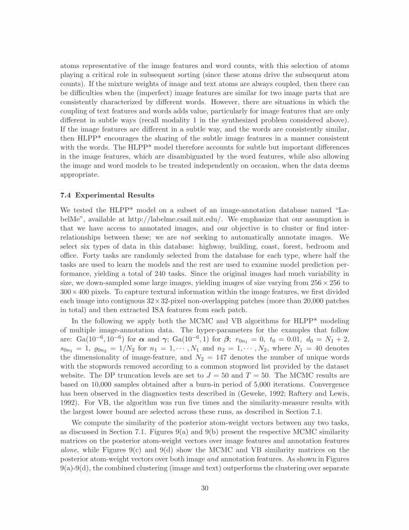
atoms representative of the image features and word counts, with this selection of atomsplaying a critical role in subsequent sorting (since these atoms drive the subsequent atomcounts). If the mixture weights of image and text atoms are always coupled, then there canbe difficulties when the (imperfect) image features are similar for two image parts that areconsistently characterized by different words. However, there are situations in which thecoupling of text features and words adds value, particularly for image features that are onlydifferent in subtle ways (recall modality 1 in the synthesized problem considered above).If the image features are different in a subtle way, and the words are consistently similar,then HLPP* encourages the sharing of the subtle image features in a manner consistentwith the words. The HLPP* model therefore accounts for subtle but important differencesin the image features, which are disambiguated by the word features, while also allowingthe image and word models to be treated independently on occasion, when the data deemsappropriate.
7.4 Experimental Results
We tested the HLPP* model on a subset of an image-annotation database named “La-belMe”, available at http://labelme.csail.mit.edu/. We emphasize that our assumption isthat we have access to annotated images, and our objective is to cluster or find inter-relationships between these; we are not seeking to automatically annotate images. Weselect six types of data in this database: highway, building, coast, forest, bedroom andoffice. Forty tasks are randomly selected from the database for each type, where half thetasks are used to learn the models and the rest are used to examine model prediction per-formance, yielding a total of 240 tasks. Since the original images had much variability insize, we down-sampled some large images, yielding images of size varying from 256× 256 to300×400 pixels. To capture textural information within the image features, we first dividedeach image into contiguous 32×32-pixel non-overlapping patches (more than 20,000 patchesin total) and then extracted ISA features from each patch.
In the following we apply both the MCMC and VB algorithms for HLPP* modelingof multiple image-annotation data. The hyper-parameters for the examples that followare: Ga(10−6, 10−6) for α and γ; Ga(10−6, 1) for β; r0n1 = 0, t0 = 0.01, d0 = N1 + 2,s0n1 = 1, 0n2 = 1/N2 for n1 = 1, · · · , N1 and n2 = 1, · · · , N2, where N1 = 40 denotesthe dimensionality of image-feature, and N2 = 147 denotes the number of unique wordswith the stopwords removed according to a common stopword list provided by the datasetwebsite. The DP truncation levels are set to J = 50 and T = 50. The MCMC results arebased on 10,000 samples obtained after a burn-in period of 5,000 iterations. Convergencehas been observed in the diagnostics tests described in (Geweke, 1992; Raftery and Lewis,1992). For VB, the algorithm was run five times and the similarity-measure results withthe largest lower bound are selected across these runs, as described in Section 7.1.
We compute the similarity of the posterior atom-weight vectors between any two tasks,as discussed in Section 7.1. Figures 9(a) and 9(b) present the respective MCMC similaritymatrices on the posterior atom-weight vectors over image features and annotation featuresalone, while Figures 9(c) and 9(d) show the MCMC and VB similarity matrices on theposterior atom-weight vectors over both image and annotation features. As shown in Figures9(a)-9(d), the combined clustering (image and text) outperforms the clustering over separate
30
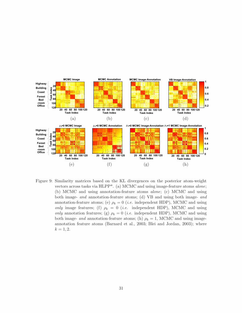
Highway
Building
Coast
Forest
Bed
-roomOffice
Task Index
TaskIndex
MCMC Image
20 40 60 80 100120
20
40
60
80
100
120
Task Index
MCMC Annotation
20 40 60 80 100120
MCMC Image-Annotation
Task Index20 40 60 80 100120
VB Image-Annotation
Task Index20 40 60 80 100120
0.2
0.4
0.6
0.8
1
(a) (b) (c) (d)
Task Index
TaskIndex
20 40 60 80 100 120
20
40
60
80
100
120
Highway
Building
Coast
Forest
Bed
-roomOffice
rk=0 MCMC Image
Task Index20 40 60 80 100 120
rk=0 MCMC Annotation
Task Index20 40 60 80 100 120
=0 MCMC Image-Annotationrk
Task Index20 40 60 80 100 120
0
0.2
0.4
0.6
0.8
1=1 MCMC Image-Annotationrk
(e) (f) (g) (h)
Figure 9: Similarity matrices based on the KL divergences on the posterior atom-weightvectors across tasks via HLPP*. (a) MCMC and using image-feature atoms alone;(b) MCMC and using annotation-feature atoms alone; (c) MCMC and usingboth image- and annotation-feature atoms; (d) VB and using both image- andannotation-feature atoms; (e) ρk = 0 (i.e. independent HDP), MCMC and usingonly image features; (f) ρk = 0 (i.e. independent HDP), MCMC and usingonly annotation features; (g) ρk = 0 (i.e. independent HDP), MCMC and usingboth image- and annotation-feature atoms; (h) ρk = 1, MCMC and using image-annotation feature atoms (Barnard et al., 2003; Blei and Jordan, 2003); wherek = 1, 2.
31

image-feature atoms or annotation-feature atoms. For comparison, Figures 9(e)-9(h) presentthe corresponding similarity matrices across tasks generated using two extremes of HLPP*:i) ρk = 0, and ii) ρk = 1, for k = 1, 2. We note that case i) corresponds to treating the imageand text features independently in the prior; while case ii) corresponds to the situation inwhich the mixture weights of image and text atoms are always the same, as in (Barnardet al., 2003; Blei and Jordan, 2003). Figures 9(e) and 9(f) only use image features and textfeatures, respectively; Figure 9(g) uses both of the posterior atom-weight vectors via themodels of Figures 9(e) and 9(f) to yield the combined similarity matrix (as discussed inSection 7.3).
To provide more-quantitative comparisons, Figure 10 directly compares the correct clus-tering rates of the above eight methods over categories. In Figure 10 each bar reflects theaverage fraction of the top-19 closest members of each task’s ordered similarity list that arewithin the same category as the task under test (there are 20 examples in each category;therefore, this measure examines the degree to which a given data is deemed most similarto all other data within the same class, before being similar to data from any other class).It is clear from Figure 10 that ordering based on atom information from both the imageand text features yields best performance, and generally the MCMC and VB HLPP* im-plementations provide similar performance. Typical example sorting results are depicted inFigure 11. Considering Figure 10 more carefully, we note that in some cases using ρk = 1 fork = 1, 2 (Barnard et al., 2003; Blei and Jordan, 2003) yields significantly worse clusteringperformance than HLPP*, in particular for Building, Coast, Forest, Office and Bedroom.Additionally, in some cases using ρk = 0 for k = 1, 2 (treating the image and text featuresindependently in the prior) and employing both of the posterior atom-weight vectors to mea-sure similarity actually does better than directly coupling the mixture weights in the prior,in particular for Coast, Forest, Bedroom and Office, with this attributed to imperfectionsin the image features and in the annotations.
To demonstrate the prediction performance of the HLPP* model, Figure 12 reportsthe correct clustering rates for test data (now based on the average fraction of the top-10closest members of the ranking list for each data); here we only show the top-10 (rather than19) because these samples were not in the training set. From the results shown in Figure12, we observe that MCMC and VB using the posterior atom-weight vectors over bothimage and annotation features achieved good test results for highway, building, coast andforest categories (larger than 0.85). Since the bedroom and office categories are somewhatconfused in the training procedure, their test results are also not as good as those of othercategories (about 0.75). Nevertheless, these are only clustering results; it is anticipatedthat one may design classifiers based on the posterior atom-weight vectors to improve thetest performance (in future work). In addition, the results using the posterior atom-weightvectors over image features and annotation features alone are also good (see Figure 12).This demonstrates that our model may also be used for automatic annotation and text-basedimage retrieval.
The computation required for learning the models via MCMC is expensive: it requiredover 48 hours (for the burn-in and collection period given above), using non-optimizedMatlabTM software on a Pentium IV PC with a 2.1 GHz CPU. By contrast, the VB solutionis much faster, requiring less than 4 hours, with typically about 50 iterations needed forconvergence. For both versions, the testing on new data in the sense discussed in Section 7.1
32

Highway Building Coast Forest Bedroom Office0
0.2
0.4
0.6
0.8
1
1.2
1.4
Category Index
Cor
rect
Clu
ster
ing
Rat
es fo
r T
rain
ing
Dat
a
MCMC Image
MCMC Annotation
MCMC Image−Annotation
VB Image−Annotation
ρk=0 MCMC Image
ρk=0 MCMC Annotation
ρk=0 MCMC Image−Annotation
ρk=1 MCMC Image−Annotation
Figure 10: Each bar reflects the average fraction of the top-19 closest samples that arewithin the same category as the sample under test (there are 20 examples ineach category). The ranking is based on the KL divergences on the posterioratom-weight vectors. Unless specified, the results are based on MCMC. TheHLPP* results are computed via the posterior weights on image-feature atomsalone, annotation-features atoms alone, and both image-feature and annotation-feature atoms. The results in two limiting regimes of the HLPP* model withrespect to ρk
2k=1 are also shown, where ρk = 0 for k = 1, 2 corresponds to
treating the image and text features independently in the prior; ρk = 1 fork = 1, 2 corresponds to the situation in (Barnard et al., 2003; Blei and Jordan,2003)
33

sky, trees, trees, sign, sign, ground
grass, central reservation, car, van,
sign, road
Hig
hway
reference
sky, road, central reservation, sign,
hedge, car, car, trees, trees, road
1
sky, trees, bridge, road, central
reservation, trees, road, car, car, sign
2
desk, chair, keyboard, screen
15
sky, building, spotlight, spotlight,
spotlight, ground grass, car, tree,
tree, tree, pole, tree, tree, sidewalk,
streetlight, pole, pole, road
Bui
ldin
g
reference
sky, flag, flag, flag, flag, building,
garden, tree, plants, sidewalk, road,
sidewalk, pole, pole, pole
1
sky, dome, building, sidewalk,
pedestal, bust, door, door, door,
arcade, window, road, ground grass,
ground grass, sidewalk
2
sky, sign, sign, trees, sign, trees, car,
car, pole, pole, building, streetlight,
sidewalk, car, car, car, car, road,
central reservation, road
9
sand beach, sky, sea water, tree
Co
ast
reference
sky, building, mountain, rock, sea
water, sand beach, rock
1
sky, rocks, rock, sea water, sand
beach, person walking, sea water,
sand beach
2
sky, mountain, path, shrubs, sky,
land, tree, tree trunk, tree trunk, trees
9
fence, trees, ground, trees
Fore
st
reference
water river, sky, trees
1
trees, trees, trees
2
sky, sign, trees, fence, bridge, trees,
sign, car, car, road
17
lamp, drawer, window, pillow, rug,
wicker basket, bed, chair
reference
Bedro
om
bed, window, window, painting, tv,
pillow, pillow, tvtable, heat, plant,
commode, table
1
bed, table, table, lamp, lamp, lamp,
curtain, curtain, window, chair, glass,
painting, painting
2
monitor, chair, window
6
bookshelf, desk, desk, keyboard,
cpu, cpu, screen
Offic
e
reference
chair, desk, bookshelf, chair, screen
1
desk, chair, keyboard, screen
2
bed, lamp, painting, window,
commode, pillow, table
16
Figure 11: Typical example sorting results based on VB HLPP*; those for the MCMCinference are similar. The results are based on the posterior atom-weight vectorsover both image and annotation features. Each row is for one category. The firstcolumn shows one template sample, and the next three columns show examples ofranked sorting results, with the number above the image specifying the closenessrank order as computed by the KL divergences. The last column denotes thefirst sample in the ranking that was in a wrong category.
34

is fast (a few minutes in non-optimized MatlabTM). This is important for online informationretrieval application.
8. Conclusion
We have developed a new hierarchical Bayesian model for hybrid multi-task learning usingthe LPP prior (Dunson). The LPP prior can combine global and local clusterings through alocally-weighted mixture, and therefore it leads to dependent local clustering and borrowingof information among different modalities. In order to extend LPP to model multiple infinitemixture models, the DP-type local and global components in the original LPP model havebeen replaced with the HDP, yielding the proposed HLPP model. This model shares dataacross multiple modalities and multiple tasks. Inference is performed via the combinationof collapsed and blocked Gibbs sampling and VB scheme.
The performance of HLPP model has been demonstrated using a simulated example,gene-expression data, and image-annotation analysis. Compared with independent HDPmodels for the different modalities and a completely dependent HDP model for combiningthe multiple modalities, the HLPP model has demonstrated improved clustering perfor-mance. In addition, the HLPP model can provide a smaller estimation uncertainty for mostparameters, which is attributed to proper global and local sharing explicitly imposed withinthe HLPP prior. In addition, the developed VB solution allows relatively fast computation,which can be used for modeling and sorting large databases, such as the application of theimage retrieval system.
Highway Building Coast Forest Bedroom Office0
0.2
0.4
0.6
0.8
1
Category Index
Cor
rect
Clu
ster
ing
Rat
es fo
r T
est D
ata
HLPP−2 ImageHLPP−2 AnnotationHLPP−2 Image−AnnotationVB HLPP−2 Image−Annotation
Figure 12: Using a separate set of data for testing the models, each bar reflects the aver-age fraction of the top-10 closest samples that are within the same category asthe sample under test (there are 20 examples in each category). The rankingis based on the KL divergences on the posterior atom-weight vectors. The re-sults are computed via the HLPP* inferred posterior weights on image-featureatoms alone, annotation-feature atoms alone, and both the image-feature andannotation-feature atoms. The first three results are for MCMC inference, andthe last one for VB.
35

Concerning future work, there may be other forms of prior information that one maywish to impose. For example, in the time-evolving gene-expression example, the differenttasks corresponded to data collected at known time points. Typically one might expect thelikelihood of task clustering to enhance as the tasks become more proximate. Related ideashave been considered recently for simpler DP-based models (Ren et al., 2008), and may alsobe considered in future work for LPP and HLPP. One may also be interested in addressingthe realistic problem for which the data from a given task is incomplete, in that not allmodalities have been employed for a given task. For the case in which such missing data ismanifested completely randomly, the model presented here may be extended directly.
In addition, there are alternative means by which to implement the basic HLPP con-struction. For example, rather than employing an HDP prior for draws of G(m) and Gk,one may alternatively employ a nested Dirichlet process (Rodrıguez et al., 2008). In sucha construction the sharing between tasks is more explicit, since one need not always sharethe same set of atoms across tasks, as in the HDP.
Appendix A.
In this appendix we prove Property i) of the HLPP model from Section 3:
Proof. If data x(m1)l3k2
and x(m2)l4k2
are contained within the same cluster, we wish it more
probable that x(m1)l1k1
and x(m2)l2k1
will be in the same cluster, for k1 6= k2, m1 6= m2, l1 ∈
1, 2, · · · , L(m1)1 , l2 ∈ 1, 2, · · · , L
(m2)1 , l3 ∈ 1, 2, · · · , L
(m1)2 and l4 ∈ 1, 2, · · · , L
(m2)2 .
Pr(θ(m1)l1k1
= θ(m2)l2k1
) =
∫ 1∑
i1=0
1∑
i2=0
Pr(θ(m1)l1k1
= θ(m2)l2k1
|z(m1)k1
= i1, z(m2)k1
= i2)
·Pr(z(m1)k1
= i1, z(m2)k1
= i2)· (ρk1) dρk1
= E[∞∑
j=1
v(m1)0j v
(m2)0j ] · E[ρ2
k1] + E[
∞∑
j=1
v(m1)k1j v
(m2)k1j ] · E[(1 − ρk1)
2]
=
∫
∞∑
j=1
E2[v(m1)0j |ω′] · E[ρ2
k1] +
∞∑
j=1
E2[v(m1)k1j |ω′] · E[(1 − ρk1)
2]
p(ω′) dω′
= E[∞∑
j=1
ω′2j
j−1∏
h=1
(1 − ω′h)2] ·
(
E[ρ2k1
] + E[(1 − ρk1)2])
=
(
1
1 + α
)(
1
2 + β
)(
β +2
1 + β
)
= P1(α, β) (40)
36
In the above derivation, since v(m)k′
i.i.d.∼ DP(α,ω), E[v
(m)k′ |ω′] = ω with ωj =
∑∞j=1 ω
′j
∏j−1h=1(1−
ω′h), for k′ = 0, 1, · · · ,K and m = 1, 2, · · · ,M .
Pr(θ(m1)l1k1
= θ(m2)l2k1
,θ(m1)l3k2
= θ(m2)l4k2
) = E[∞∑
j1=1
v(m1)0j1
v(m2)0j1
∞∑
j2=1
v(m1)0j2
v(m2)0j2
] · E[ρ2k1ρ2
k2]
+ E[
∞∑
j1=1
v(m1)0j1
v(m2)0j1
∞∑
j2=1
v(m1)k2j2
v(m2)k2j2
] · E[ρ2k1
(1 − ρk2)2]
+ E[
∞∑
j1=1
v(m1)k1j1
v(m2)k1j1
∞∑
j2=1
v(m1)0j2
v(m2)0j2
] · E[(1 − ρk1)2ρ2
k2]
+ E[∞∑
j1=1
v(m1)k1j1
v(m2)k1j1
∞∑
j2=1
v(m1)k2j2
v(m2)k2j2
] · E[(1 − ρk1)2(1 − ρk2)
2]
=
∞∑
j1=1
E[(
ω′2j1
+ Var[v(m1)0j1
|ω′])2
j1−1∏
h1=1
(
(
1 − ω′h1
)2+ Var[v
(m1)0h1
|ω′])2
]
+
∞∑
j1=1
E[ω′2j1
j1−1∏
h1=1
(1 − ω′h1
)2]∑
j2:j2 6=j1
E[ω′2j2
j2−1∏
h2=1
(1 − ωh2)′2]
· E2[ρ2k1
]
+ E[
∞∑
j1=1
ω′2j1
j1−1∏
h1=1
(1 − ω′h1
)2
2
] ·
2E[ρ2k1
] · E[(1 − ρk1)2] + E2[(1 − ρk1)
2]
= P2(α, β, γ)
=
E[
∞∑
j1=1
ω′2j1
j1−1∏
h1=1
(1 − ω′h1
)2
2
]
·
E2[ρ2k1
] + 2E[ρ2k1
] · E[(1 − ρk1)2] + E2[(1 − ρk1)
2]
+
∞∑
j1=1
E[Var2[v(m1)0j1
|ω′]
j1−1∏
h1=1
(
(1 − ω′h1
)2 + Var[v(m1)0h1
|ω′])2
+ 2ω′2j1
Var[v(m1)0j1
|ω′]
·
j1−1∏
h1=1
(
(1 − ω′h1
)2 + Var[v(m1)0h1
|ω′])2
+ ω′4j1
j1−1∏
h1=1
Var2[v(m1)0h1
|ω′]]
· E2[ρ2k1
]
= P2,1(α, β) + P2,2(α, β, γ)
=6 + α
(1 + α)(2 + α)(3 + α)
[
4
(1 + β)2(2 + β)2+
2 × 2
(1 + β)(2 + β)
(
β
2 + β
)
+
(
β
2 + β
)2]
+ P2,3(α, γ)4
(1 + β)2(2 + β)2
=6 + α
(1 + α)(2 + α)(3 + α)(2 + β)2
(
β +2
1 + β
)2
+4P2,3(α, γ)
(1 + β)2(2 + β)2
37

P2,1(α, β) = E[
∞∑
j1=1
ω′2j1
j1−1∏
h1=1
(1 − ω′h1
)2
2
]
·
E2[ρ2k1
] + 2E[ρ2k1
] · E[(1 − ρk1)2] + E2[(1 − ρk1)
2]
P2,2(α, β, γ) = P2,3(α, γ) · E2[ρ2
k1]
P2,3(α, γ) =
∞∑
j1=1
E[Var2[v(m1)0j1
|ω′]
j1−1∏
h1=1
(
(1 − ω′h1
)2 + Var[v(m1)0h1
|ω])2
+ 2ω′2j1
Var[v(m1)0j1
|ω′]
·
j1−1∏
h1=1
(
(1 − ω′h1
)2 + Var[v(m1)0h1
|ω′])2
+ ω′4j1
j1−1∏
h1=1
Var2[v(m1)0h1
|ω′]]
Var[v(m1)0j1
|ω′] =ω′
j1− ω
′2j1
γ∏j1−1
h1=1(1 − ω′h1
) + 1
Since Var[v(m1)0j1
|ω′] ≥ 0, P2,2(α, β, γ) ≥ 0 (while there is no analytical solution for P2,3(α, γ)).
We can easily proveP2,1(α,β)P1(α,β) ≥ P1(α, β), and then P2(α,β,γ)
P1(α,β) ≥ P1(α, β), therefore, Property1 in Section 3 is satisfied.
Appendix B.
In this appendix we prove the Property ii) of the HLPP model from Section 3:
Proof. Note that
Pr([
Pr(θ(m1)l1k1
= θ(m2)l2k1
|θ(m1)l3k2
= θ(m2)l4k2
) − Pr(θ(m1)l1k1
= θ(m2)l2k1
)]
∈ S)
=
∫
1(
∆(α, β, γ) ∈ S)
F(α, β, γ) dα dβ dγ (41)
where ∆(α, β, γ) = P2(α, β, γ)/P1(α, β) − P1(α, β), and F(α, β, γ) is the prior density forα, β and γ. Since we use independent gamma priors, F(α, β, γ) > 0 for all (α, β, γ) ∈(0,∞) × (0,∞) × (0,∞). For any point ι ∈ S, there exists a corresponding region ϑ(ι) ⊂(0,∞)× (0,∞)× (0,∞) of (α, β, γ) values that result in ∆(α, β, γ) = ι, with ϑ(ι) 6= ∅ for allι ∈ (0, 1). This condition follows directly if there exists an (α, β, γ) solution to the equation∆(α, β, γ) = ι, for every point ι in 0 < ι < 1. According to (40) and (??)
∆(α, β, γ) =2α
(1 + α)(2 + α)(3 + α)
β2 + β + 2
(1 + β)(2 + β)+
4(1 + α)P2,3(α, γ)
(1 + β)(2 + β)(β2 + β + 2)(42)
If α→ 0 and γ → ∞, then ∆(0, β,∞) → 0. When α→ ∞ and β → 0, we can simplify theHLPP model and easily obtain
Pr(θ(m1)l1k1
= θ(m2)l2k1
) → 0, Pr(θ(m1)l1k1
= θ(m2)l2k1
|θ(m1)l3k2
= θ(m2)l4k2
) → 6+γ(2+γ)(3+γ) (43)
Thus ∆(∞, 0, γ) → (6+γ)/ [(2 + γ)(3 + γ)]. If γ → 0, then ∆(∞, 0, 0) → 1. Since ∆(α, β, γ)should be a continuous function, Pr (∆(α, β, γ) ∈ S) > 0 for all Borel subset S ⊂ [0, 1].
38
References
E. M. Airoldi, D. M. Blei, S. E. Fienberg, and E. P. Xing. Mixed membership stochasticblockmodels. Journal of Machine Learning Research, 9:1981–2014, 2008.
Q. An, C. Wang, I. Shterev, E. Wang, D. B. Dunson, and L. Carin. Hierarchical kernel stick-breaking process for multi-task image analysis. In International Conference of MachineLearning (ICML), 2008.
K. Barnard, P. Duygulu, N. de Freitas, D. Forsyth, D. M. Blei, and M. I. Jordan. Matchingwords and pictures. Journal of Machine Learning Research, 3:1107–1135, 2003.
M. J. Beal. Variational algorithms for approximate Bayesian inference. PhD thesis, GatsbyComputational Neuroscience Unit, University College London, 2003.
D. Blei, A. Ng, and M. Jordan. Latent dirichlet allocation. Journal of Machine LearningResearch, 3:993–1022, 2003.
D. M. Blei and M. I. Jordan. Modeling annotated data. In Proceedings of the 26th an-nual international ACM SIGIR conference on Research and development in informationretrieval, pages 127–134, 2003.
E. Brochu, N. de Freitas, and K. Bao. The sound of an album cover: Probabilistic multi-media and ir. In Ninth International Workshop on Artificial Intelligence and Statistics,2003. URL http://www.cs.ubc.ca/ nando/papers/aismedia.pdf.
C. Carvalho, J. Chang, J. Lucas, J. R. Nevins, Q. Wang, and M. West. High-dimensionalsparse factor modeling: applications in gene expression genomics. Journal of the AmericanStatistical Association.
J. T. Chang and J. R. Nevins. Sgather: a systems approach to interpreting genomic signa-tures. Bioinformatics, 22(23):2926–2933, 2006.
P. Common. Independent component analysis - a new concept? Signal Processing, 36:287–314, 1994.
D. B. Dunson. Nonparametric bayes local partiotion models for random effects. Biometrika.
D. B. Dunson, Y. Xue, and L. Carin. The matrix stick-breaking process: Flexible bayesmeta analysis. Journal of the American Statistical Association, 103:317–327, 2008.
J. Fink, F. Gu, L. Ling, T. Tolfvenstan, F. Olfat, K. C. Chin, P. Aw, J. George, V. A.Kuznetsov, M. Schreiber, S. G. Vasudevan, and M. L. Hibberd. Host gene expressionprofiling of dengue virus infection in cell lines and patients. PLoS Neglected TropicalDiseases, 1(2), 2007.
E. Fokoue. Stochastic determination of the intrinstic structure in bayesian factor analysis.Technical report, 2004.
J. Geweke. Evaluating the accuracy of sampling-based approaches to calculation of posteriormoments. Bayesian Statistics, 4:169–193, 1992.
39

W. R. Gilks and D. J. Spiegelhalter. Markov Chain Monte Carlo in Practice. London:Chapman Hall, 1996.
T. L. Griffiths and Z. Ghahramani. Infinite latent feature mod-els and the indian buffet process. Technical report, 2005. URLhttp://cocosci.berkeley.edu/tom/papers/ibptr.pdf.
P. Hoyer and A. Hyvarinen. Independent component analysis applied to feature extractionfrom colour and stereo images. Network: Computation in Neural Systems, 11(3):191–210,2000.
A. Hyvarinen and P. Hoyer. Emergence of phase- and shift-invariant features by decompo-sition of natural images into independent feature subspace. Neural Computation, 12(7):1705–1720, 2000.
H. Ishwaran and L. F. James. Gibbs sampling methods for stick-breaking priors. Journalof the American Statistical Association, 96:161173, 2001.
J. Jeon, V. Lavrenko, and R. Manmatha. Automatic image annotation and retrieval usingcross-media relevance models. In Proceedings of the 26th annual international ACMSIGIR conference on Research and development in informaion retrieval, pages 119–126,2003.
C. Kemp, T. L. Griffiths, and J. B. Tenenbaum. Discovering latent classes in relationaldata. Technical report, 2004.
C. Kemp, J. B. Tenenbaum, T. L. Griffiths, T. Yamada, and N. Ueda. Learning systems ofconcepts with an infinite relational model. In Proceedings of the 21st National Conferenceon Artificial Intelligence, 2006.
D. Knowles and Z. Ghahramani. Infinite sparse factor analysis and infinite independentcomponents analysis. In 7th International Conference on Independent Component Anal-ysis and Signal Separation (ICA), 2007.
K. Livescu, K. Sridharan, S. Kakade, and K. Chauduri. Multi-view clustering via canonicalcorrelation analysis. In Neural Information Processing Systems Conference, 2008.
S. N. MacEachern. Estimating mixture of dirichlet process models. Journal of Computa-tional and Graphical Statistics, 7:223–238, 1998.
P. Muliere and L. Tardella. Approximating distributions of random functionals of ferguson-dirichlet priors. Can. J. Statist., 26:283–97, 1998.
S. Petrone, M. Guindani, and A. E. Gelfand. Hybrid dirichlet processesfor functional data. In An Isaac Newton Institute Workshop: Construc-tion and Proferties of Bayesian Nonparametric Regression Models, 2008. URLhttp://www.newton.ac.uk/programmes/BNR/seminars/080811301.html.
I. Pournara and L. Wernish. Factor analysis for gene regulatory networks and transcriptionfactor activity profiles. BMC Bioinformatics, 8, 2007.
40

A. E. Raftery and S. Lewis. How many iterations in the gibbs sampler? Bayesian Statistics,4:763–773, 1992.
L. Ren, D. B. Dunson, and L. Carin. The dynamic hierarchical dirichlet process. InInternational Conference of Machine Learning (ICML), 2008.
A. Rodrıguez, D. B. Dunson, and A. E. Gelfang. The nested dirichlet process. Journal ofthe American Statistical Association, 103:1131–1144, 2008.
B. Taskar, E. Segal, and D. Koller. Probabilistic clustering in relational data. In IJCAI-01,pages 870–876, 2001.
Y. W. Teh, M. I. Jordan, M. J. Beal, and D. M. Blei. Hierarchical dirichlet processes.Journal of the American Statistical Association, 101(476):1566–1581, 2006.
Y. W. Teh, K. Kurihara, and M. Welling. Collapsed variational inferencefor hdp. In Neural Information Processing Systems Conference, 2007. URLhttp://www.ics.uci.edu/ welling/publications/papers/CVHDP.pdf.
S. G. Walker. Sampling the dirichlet mixture model with slices. Comm. Statist. Sim.Comput., 36:45–54, 2007.
Y. J. Wang and G. Y. Wong. Stochastic blockmodels for directed graphs. Journal of theAmerican Statistical Association, 82:819, 1987.
F. Wood, T. L. Griffiths, and Z. Ghahramani. A non-parametric bayesian method forinferring hidden causes. In Uncertainty in Artificial Intelligence (UAI), pages 536–543,2006.
Z. Xu, V. Tresp, K. Yu, and H. Kriegel. Learning infinite hidden relational models. InUncertainty in Artificial Intelligence (UAI), 2006.
Y. Xue, X. Liao, L. Carin, and B. Krishnapuram. Multi-task learning for classification withdirichlet process priors. Journal of Machine Learning Research, 8:35–63, 2007.
41
![Blinder: Partition-Oblivious Hierarchical Scheduling › system › files › sec21summer_yoon.pdfof ARINC 653 standard [8] and MILS systems employ this table-driven approach as the](https://img.pdfslide.net/doc/110x75/60b717e16d94d36f9c53b64a/blinder-partition-oblivious-hierarchical-scheduling-a-system-a-files-a-sec21summeryoonpdf.jpg)