The Historical Evolution of the Wealth Distribution: A

Quantitative-Theoretic Investigation

Joachim Hubmer, Per Krusell, and Anthony A. Smith, Jr.∗

August 9, 2017

Abstract

This paper employs the benchmark heterogeneous-agent macroeconomic model to examine drivers

of the rise in wealth inequality in the U.S. over the last thirty years. By far the most important driver

is the significant drop in tax progressivity starting in the late 1970s. The sharp observed increases in

earnings inequality and the falling labor share over the recent decades, on the other hand, fall far short

of accounting for the data. Changes in asset returns and in the inflation rate help to account for the

shorter-run dynamics in wealth inequality.

1 Introduction

The distribution of wealth in most countries for which there is reliable data is strikingly uneven. There is

also recent work suggesting that the wealth distribution has undergone significant movements over time,

most recently with a large upward swing in dispersion in several Anglo-Saxon countries.1 For example,

according to the estimates in Saez & Zucman (2016) for the United States, the share of overall wealth

held by the top 1% has increased from around 25% in 1980 to over 40% today; for the top 0.1% it has

increased from less than 10% to over 20% over the same time period.

The observed developments have generated strong reactions across the political spectrum. In his 2014

book, Capital in the Twenty-First Century , Piketty is obviously motivated by the growing inequality

in itself, but he also suggests that further increases in wealth concentration may lead to both economic

and democratic instability. Conservatives in the U.S. have expressed worries as well: is the American

Dream really still alive, or might it be that a large fraction of the population simply will no longer be

able to productively contribute to society? Given, for example, that parental wealth and well-being are

important determinants behind children’s human capital accumulation, this appears to be a legitimate

concern regardless of one’s political views. As a result of these concerns, a number of policy changes have

∗The authors’ affiliations are, respectively, Yale University; Institute for International Economic Studies, NBER, andCEPR; and Yale University and NBER. For helpful comments the authors would like to thank Chris Carroll, Harald Uhlig,and seminar participants at the 2015 SED Meetings, the 2015 Hydra Workshop on Dynamic Macroeconomics, the SeventhMeeting of the Society for the Study of Economic Inequality, the 2017 NBER Summer Institute, Johns Hopkins, Indiana,M.I.T., Penn State, University of Pennsylvania, SOFI, and Yale.

1See, e.g., Piketty (2014) and Saez & Zucman (2016).

1

been proposed and discussed. The primary aim of the present paper is to understand the determinants of

the observed movements in wealth inequality. This aim is basic but well-motivated: to compare different

policy actions, we need a framework for thinking about what causes inequality and for addressing how

inequality—and other variables—are influenced by any policy proposal at hand.

In an effort to understand the movements in wealth inequality, Piketty (2014) and its online appendix

suggest specific mathematical theories and as part of the present study we examine those theories.2 Our

aim, however, is to depart instead from a more general, and by now rather standard, quantitatively

oriented theory used in the heterogeneous-agent literature within macroeconomics: the Bewley-Huggett-

Aiyagari model. This is a very natural setting for the study of inequality. This model incorporates rich

detail on the household level along the lines of the applied work in the consumption literature, allowing

several sources of heterogeneity among consumers. It is based on incomplete markets and, hence, does not

feature the “infinite elasticity of capital supply” of dynastic models with complete markets.3 This model

also involves equilibrium interaction: inequality is determined not only by the individual household’s

reactions to changes in the economic environment in which they operate but also by their interaction,

such as in the equilibrium formation of wages and interest rates, two key prices determining the returns to

labor and holding wealth, respectively. Our aim is to see to what extent a reasonably calibrated model can

account for the movements in wealth inequality from the mid-1960s and on as a function of a number of

drivers, the importance of each of which we then evaluate in separate counterfactuals.4 In this endeavor,

we proceed as follows.

We build on the model studied in Aiyagari (1994), i.e., we use the core setting of the recent literature

on heterogenous agents in macroeconomics.5 This kind of theoretical model is quantitative in nature: it

is constructed as an aggregate version of the applied work on consumption. Moreover, in it, inequality

plays a central role. We calibrate some key parameters of this model to match the wealth and income

distributions in the United States in the mid-1960s and treat these distributions as representing a long-run

steady state. In the 1960s, too, the dispersion of wealth was striking, and it is not immediate how to make

the basic model match the data in this respect. Building on the formulation in Krusell & Smith (1998), we

use preference heterogeneity—in particular, stochastic discount rates that vary across the population at

a point in time—to generate individual behavior among the very richest characterized by propensities to

save that are stochastic but (almost completely) independent of wealth. We also incorporate idiosyncratic

random asset returns, for which recent work by Fagereng et al. (2015) and Bach et al. (2015) uncovers

evidence in panel data from Norway and Sweden. Hence, our setting can be viewed as a microfoundation

for the kind of models entertained in Piketty & Zucman (2015) (who assume linear laws of motion for

wealth accumulation and either random saving propensities or random returns). These models generate a

wealth distribution whose right tail is Pareto-shaped, a feature shown to characterize the data; we discuss

2The appendix is available here: http://piketty.pse.ens.fr/files/capital21c/en/Piketty2014TechnicalAppendix.pdf. Seealso Piketty (1995) and Piketty (1997) which develop theories of the dynamics of the wealth distribution.

3This elasticity refers to the long-run response of a household’s savings to a change in the interest rate: in particular, withinfinitely-lived consumers and complete markets the equilibrium interest rate is pinned down by the rate of time preference.

4We do not specifically study Piketty’s “Second Fundamental Law”, which is not a theory about inequality per se butabout the aggregate capital-output ratio and which has also been extensively examined in Krusell & Smith (2015).

5The first application in this literature was one to asset pricing (the risk-free rate): Huggett (1993). Aiyagari (1994)addresses the long-run level of precautionary saving, whereas Krusell & Smith (1998) look at business cycles.

2

this finding and the relation to a number of other papers building on the same kind of reduced form in

detail in the paper.

With the resulting realistic starting wealth distribution, we then examine a number of potential drivers

of wealth inequality over the subsequent period. One is tax rates: beginning around 1980 tax rates fell

significantly for top incomes, so that tax progressivity in particular fell substantially. Thus, higher returns

to saving in the upper brackets since that time can potentially explain increased wealth gaps between the

rich and the poor. Another potential explanation for increased wealth inequality is the rather striking

increases in wage/earnings inequality witnessed since the mid-1970s. Since at least Katz & Murphy (1992)

it has been well-documented that the education skill premium has risen. Moreover, numerous studies have

since documented that the premia associated with other measures of skill have also risen, as have measures

of residual, or frictional, wage dispersion.6 In terms of the very highest earners, Piketty & Saez (2003)

document significant movements toward thicker tails in the upper parts of the distribution. So to the

extent that this increased income inequality has translated into savings and wealth inequality, it could

explain some of the changes we set out to analyze. Relatedly, the share of total income paid to capital

has increased recently, potentially contributing to increased wealth inequality (see, e.g., Karabarbounis

& Neiman (2014b)). We consider this factor as well in this study.

Thus, the overall methodology we follow is to attempt to quantify the mechanisms just mentioned and

then to examine their individual (and joint) effects on the evolution of wealth inequality from the 1960s.

For the time period considered, we find that the benchmark model does account for a significant share of

the increase in wealth inequality. The model is more or less successful depending on what aspect of the

wealth distribution is in focus. The shares of wealth held by the top 10% or top 1% exhibit net increases

that are very similar in the model and in the data, though for the top 0.1% and 0.01% the model does

not deliver enough of an increase, especially for the very top group. For the bottom 50%, the model’s

fit is also good. Furthermore, the model delivers a time path for the ratio of capital to net output that

is similar to the one in the data. As for the timing of the changes, the model delivers a rather smooth

increase in inequality, whereas the data shows faster swings, first down and then up (the model generates

a visible, though gentle, kink of this sort too, but in growth rates).

Turning to which specific features explain the largest fractions of the increase in wealth inequality, the

marked decrease in tax progressivity is by far the most powerful force for increasing wealth inequality.7

First, other things equal, decreasing tax progressivity spreads out the distribution of after-tax resources

available for consumption and saving. Second, decreasing tax progressivity increases the returns on

savings, leading to higher wealth accumulation, especially among the rich for whom wages (earnings) is a

smaller part of wealth.

Wage inequality, on the other hand, on net contributes negatively to wealth inequality: it increases

by more in a model with changes in progressivity unaccompanied by increases in wage inequality than

in a model with both types of changes. We follow Heathcote et al. (2010) in modelling increased wage

inequality as an increase in the riskiness of wage realizations around a mean. In a standard additive

permanent-plus-transitory model of wages, we use the estimated time series in Heathcote et al. (2010) for

6See, e.g., Acemoglu (2002), Hornstein et al. (2005), and Quadrini & Rios-Rull (2015).7These conclusions are line with two studies of France and the U.S.: Piketty (2003) and Piketty & Saez (2003).

3

the variances of the permanent and transitory shocks to wages. Both of those variances have increased

over time, leading to a reduction in wealth inequality for two reasons. First, increasing wage risk dampens

the tendency of heterogeneity in discount rates to drive apart the distribution of wealth.8 In particular, as

wage risk increases, poorer and less patient consumers—who are less well-insured against this risk through

their own savings—engage in additional precautionary saving, compressing the distribution of wealth at

the low end. Second, with more risk aggregate precautionary savings increase, reducing the equilibrium

interest rate and reducing the relative wealth accumulation of the rich, for whom wage risk is also not so

important. In sum, the increasing riskiness of wages compresses the wealth distribution at both ends.9

In addition, we follow Piketty & Saez (2003) by adding a Pareto-shaped tail to the wage distribution

so as to match the concentration of earnings at the top of the earning distribution; the standard wage

process (as in Heathcote et al. (2010)) does not match this extreme right tail well. Moreover, the right

tail has thickened over this period, and accordingly we model this thickening as a gradually decreasing

Pareto coefficient, based on the estimates in Piketty & Saez (2003). This element of increased wage

inequality does generate more wealth inequality—because it occurs in a segment of the population where

most workers are already rather well-insured through their own savings—but it is not so potent as to

produce a net overall increase in wealth inequality from higher wage inequality. To allow for an increasing

capital share over time we conduct an experiment using a CES production function with a somewhat

higher than unitary elasticity between capital and labor. The resulting paths in this experiment differ

only marginally from the case with unitary elasticity.

Given that the model predicts the within-period swings in the wealth shares less well than over the

full period, we also begin a preliminary examination of the effects of systematic return differences on the

overall portfolio between the poor and the rich. We look at both stock-market valuation effects—the idea

being that the rich hold a larger fraction of stock than do the poor—and inflation effects, where we point

out that progressivity jointly with a tax schedule that is not indexed to inflation reduces the returns to

saving of the wealthy more than it does for the poor if inflation rises.10 These factors both turn out to

have direct effects that are sizable, so this line of research seems promising. We restrict attention here,

however, to hard-wired portfolio-share differences and do not allow a nominal-vs.-real asset choice, and

we moreover take returns as given and thus use a partial-equilibrium setting. Hence, a deeper foray into

these issues seems promising but must be left for future work.

What are the implications of our dynamic model of wealth inequality for the future? Quite strikingly,

if the progressivity of taxes remains at today’s historically low level, then wealth inequality will continue

to climb and reach very high levels by, say, 2100: the top 10% will have an additional 10% of all of wealth,

as will (approximately) the top 1%. Thus, decreasing the progressivity of taxes is a rather powerful

mechanism for wealth concentration. In this context, we also consider a possible long-run decline in the

8As Becker (1980) shows, if discount rates are permanently different and there is no wage risk at all, then in the long-runsteady state the most patient consumer owns all of the economy’s wealth.

9Similar forces are at play in Krusell et al. (2009), but in the opposite direction: they find that reductions in wage riskthat accompany the elimination of business cycles lead to higher wealth inequality.

10This channel is thus not the same as general bracket creep but rather appears due to the interaction between nominaltaxation and progressivity: even if inflation makes no single consumer creep up a bracket, it makes the net-of-tax real returnfall more for consumers in higher tax brackets.

4

rate of growth, g—a determinant in Piketty’s r − g story behind inequality in line with a recent popular

belief of “secular stagnation”—and find that, although interesting in its own right, it does not affect these

conclusions appreciably.

Our paper begins in Section 2 with a brief literature review, the purpose of which is to put our

modeling in a historical perspective. We discuss the data on wealth inequality and its recent trends in

Section 3. We describe the basic model in Section 4 and the implied behavior of the very richest in

Section 5. Section 6 discusses the calibration in detail and Section 7 the benchmark results. A number

of extensions are then included in Section 8. We conclude our paper in Section 9 with a brief discussion

of potential other candidate explanations behind the increased wealth inequality and, hence, of possible

future avenues for research.

2 Connections to the recent macro-inequality literature

The study of inequality in wealth using structural macroeconomic modeling can be said to have started

with Bewley (undated), though in Bewley’s paper the focus was not on inequality per se.11 Bewley’s

paper was not completed—it stops abruptly in the middle—and the first papers to provide a complete

analysis of frameworks like his are Huggett (1993) and Aiyagari (1994). A defining characteristic of these

models is that long-run household wealth responds smoothly to the interest rate, so long as the interest

rate is not too high (higher than the discount rate in the case without growth).

In their early papers, neither Bewley nor Huggett nor Aiyagari focused on inequality per se but rather

on other phenomena related to inequality (asset pricing and aggregate precautionary saving in the latter

two cases, respectively). Soon after, however, the macroeconomic literature that arose from these analyses

began to address inequality directly. There were several reasons for this development. One was the

interest in building macroeconomic models with microeconomic foundations in which heterogeneity could

influence aggregates, i.e., cases that are in some sense far from aggregation and the typical permanent-

income behavior that characterize the complete-markets model.12 Another was an interest in wealth

inequality per se and the challenge it posed: the difficulty that these models have in generating significant

equilibrium wealth inequality. The difficulty is apparent in Aiyagari (1994), where the wage process is

calibrated to PSID data (as an AR(1) in logs): the resulting wealth distribution is slightly more skewed

than the wage distribution the model uses as an input, but not by much. The Gini index for wealth, in

the stationary distribution of Aiyagari’s model, is only around 0.4, whereas it is around 0.8 in the data.

The purpose here is not to go over the entire literature aiming at matching the wealth distribution but

several different extensions of the model have been proposed in order to match the data better. On some

general level, successful paths forward involve introducing “more heterogeneity”: typically in preferences

(such as discount factors, as in Krusell & Smith (1998)), in the wage/earnings process (as in Castaneda

11This model is of course not the first one with theoretical implications for inequality. An early example is Stiglitz(1969) who, building on his 1966 Ph.D. dissertation, studies the dynamics of the distributions of income and wealth in aneoclassical growth model with exogenous linear savings functions. A defining characteristic of the literature in focus here isthat consumers face problems much like those studied in the applied consumption literature: they are risk-averse and chooseoptimal saving in the presence of earnings shocks for which there is not a full set of state-contingent markets.

12See, e.g., Krusell & Smith (1998) and Guerrieri & Lorenzoni (2011) for this line of work.

5

et al. (2003)), or in occupation (as in Cagetti & De Nardi (2006) or Quadrini (2000)).

More recently, a literature evolved that focuses on explaining the observed Pareto tail at the top of

the wealth distribution. Benhabib et al. (2011) show analytically that the stationary wealth distribution

in an overlapping-generations (OLG) economy with idiosyncratic capital return risk has a Pareto tail.

Analogously, they provide analytical results for an infinite-horizon economy (Benhabib et al., 2015b).

In Benhabib et al. (2015a), they conduct a quantitative investigation of social mobility and the wealth

distribution in an OLG economy with idiosyncratic returns, which are fixed over a life-time. In a stylized

model, Gabaix et al. (2016) demonstrate that the random growth mechanism that can generate the Pareto

tail in the wealth distribution (either through idiosyncratic capital return risk or random discount factors)

implies very slow transitional dynamics. Furthermore, Nirei & Aoki (2016) consider a stationary Bewley

economy with investment risk. In that setting they find that decreasing top tax rates can explain the

increasing concentration of wealth at the top.

Most of the literature on Bewley models has considered only the stationary (long-run) wealth distri-

bution. Two recent exceptions are Kaymak & Poschke (2016), who in line with our analysis here aim to

quantify the contribution of changes in taxes and transfers and in the earnings distribution to changes

in the U.S. wealth distribution, and Aoki & Nirei (forthcoming) who study how a one-time drop in tax

rates affects transitional dynamics in a setting with investment risk.

Relative to these recent contributions, the present paper builds directly on Aiyagari (1994) and matches

the wealth distribution with the aid of stochastic, heterogeneous discount rates and idiosyncratic asset

returns. As we show below, the randomness in discount rates and rates of return generates capital

accumulation dynamics for the very richest that are similar to those in the recent theoretical studies on

Pareto tails just cited, including the very slow transitional dynamics. For earnings, we follow Aiyagari

(1994) but add a transitory shock to earnings as well as an exogenous Pareto-shaped tail in earnings.

Because we also consider transitional dynamics, it is important to investigate how our results might

depend on the extent to which agents can foresee the changes in taxes and other exogenous factors; here

we consider both perfect foresight and a “myopic” alternative. We do not incorporate assets like land,

housing, or stock-market equity but focus on physical capital only. This is potentially an important

omission insofar as the returns on these assets are random and have experienced a growing variance over

time, as discussed in our concluding remarks in Section 9.

3 Measuring wealth inequality over time

Over the last century, the distribution of wealth in the United States has undergone drastic changes and

we very briefly review data from some key studies here. Throughout the time period considered, wealth

was heavily concentrated at the top. Figure 1 shows the evolution of the share of total wealth held by

the top 1% and the top 0.1%, as measured using different estimation methods.13 Considering all three

13In Figure 1, the lines labelled “SCF” display findings from the Survey of Consumer Finances, as reported in Saez &Zucman (2016). The lines labelled “Capitalization” display findings from Saez & Zucman (2016), who back out the stock ofwealth held by a tax unit from observed capital income tax data. Finally, the lines labelled “Estate tax multiplier” displayfindings from Kopczuk & Saez (2004), who use observed estate tax data to make inferences about the distribution of wealth.See Kopczuk (2015) for a detailed comparison of the different measurement methods.

6

1920 1930 1940 1950 1960 1970 1980 1990 2000 2010

Wealth S

hare

in %

5

10

15

20

25

30

35

40

45

50

55

Capitalization, Top 1%

Capitalization, Top 0.1%

SCF, Top 1%

SCF, Top 0.1%

Estate tax multiplier, Top 1%

Estate tax multiplier, Top 0.1%

Figure 1: Top wealth share measurements over time

methods jointly, top wealth inequality exhibits a U-shaped pattern in the twentieth century. Yet, the

magnitude of the increase in wealth concentration in the last thirty years differs substantially among

estimation methodologies. We will calibrate the initial steady state of our model to the wealth shares

estimated by Saez & Zucman (2016) and consequently compare the model transition to their estimates.

Their estimates are especially useful for us as they allow for considering a group as small as the top

0.01%. Furthermore, they cover a long time period. While the capitalization method that they use to

back out wealth estimates does not suffer from the shortcomings of the SCF data (such as concerns about

response-rate bias and exclusion of the Forbes 400), it is an indirect way of measuring wealth and as such

has other drawbacks. For example, the tax data allows only for a coarse partitioning of capital income

in asset classes and within each class returns are effectively assumed to be homogeneous. Since recent

evidence based on both Norwegian and Swedish data (Fagereng et al. (2015) and Bach et al. (2015),

respectively) shows significantly higher returns for the high-wealth groups, the capitalization method

suggests an over-prediction of wealth levels for the richest group. Therefore, we will in addition contrast

our findings to estimates from the Survey of Consumer Finances.14

Another takeaway from Figure 1 is that the wealth distribution was quite stable in the 1950s and

1960s. As, in addition, some of the time series estimates we feed into our model start in 1967, we take

this year as the initial steady state in our model.

14Bricker et al. (2016) make adjustments to the SCF data, including incorporating the Forbes 400. For the top 0.1% wealthshares these adjustments roughly cancel. For the top 1% shares these adjustments shift the corresponding line in Figure 1down by approximately 2 to 3 percentage points.

7

4 Model framework

In this section, we describe the model economy. We depart from the framework studied by Aiyagari

(1994). To generate realistic income and wealth heterogeneity, the model features stochastic discount

rates and returns to capital as well as an earnings process centered around a persistent and a temporary

component.

4.1 Consumers

Time is discrete and there is a continuum of infinitely lived, ex ante identical consumers (dynasties).

Preferences are defined over infinite streams of consumption with von Neumann-Morgenstern utility in

constant relative risk aversion (CRRA) form:

u(c) =c1−γ

1− γ. (1)

In period t, a consumer discounts the future with an idiosyncratic stochastic factor βt that is the realization

of a Markov process characterized by the conditional distribution Γβ(βt+1|βt), giving rise to the following

objective:

max(ct)∞t=0

{u(c0) + E0

[ ∞∑t=1

t−1∏s=0

βsu(ct)

]}. (2)

Labor supply is exogenous. Each period t, a consumer supplies a stochastic amount lt = lt(pt, νt) of

efficiency units of labor to the market that depends on a persistent component pt ∼ Γp(pt|pt−1) and a

transitory component νt ∼ Γν(νt). Taking as given a competitive wage rate wt, her earnings are wtlt.

Asset markets are incomplete: consumers cannot fully insure against idiosyncratic shocks, but instead

have access only to a single asset that pays a gross return (1+rtηt), where rt is the average market return

and ηt ∼ Γη(ηt) is a transitory idiosyncratic shock.15 We briefly discuss the challenges in endogenizing

portfolio behavior in general, and in obtaining differences in returns across consumers in particular, in

Section 8.3 below.

The decision problem of the consumer can be stated parsimoniously in recursive form:

Vt(xt, pt, βt) = maxat+1≥a

{u(xt − at+1) + βtE [Vt+1(xt+1, pt+1, βt+1)|pt, βt]} (3)

subject to xt+1 = at+1 + yt+1 − τt+1(yt+1) + Tt+1 (4)

yt+1 = rt+1ηt+1at+1 + wt+1lt+1(pt+1, νt+1) (5)

15Fagereng et al. (2015) and Bach et al. (2015) find not only heterogeneity but persistence in idiosyncratic asset returnsbut a good portion of this persistence stems from richer consumers bearing more aggregate risk, which we do not modelhere. Furthermore, given that we allow for persistence in discount factors, we find below that we can replicate the wealthdistribution in 1967, even in its remotest tails, quite accurately without persistence in idiosyncratic returns.

8

Given cash-on-hand xt (all resources available in period t), the optimal savings decision and the

resulting value function depend solely on the persistent component in the earnings process pt and the

current discount factor βt. Conditional on (pt, βt), the expectation is taken over (pt+1, βt+1) as well as

the transitory shocks to earnings νt+1 and the return on capital ηt+1. Gross income yt is subject to an

income tax τt(·) and each consumer receives a uniform lump-sum transfer Tt.

4.2 Production, government, and equilibrium

Firms are perfectly competitive and can be described by an aggregate constant returns to scale production

function F (Kt, L) that yields a wage rate per efficiency unit of labor wt = ∂F (Kt,L)∂L as well as an (average)

market return on capital rt = ∂F (Kt,L)∂K − δ, where δ ∈ (0, 1) is the depreciation rate. Aggregate labor

supply L is normalized to one throughout.

The government redistributes aggregate income by means of a uniform lump-sum payment, which

amounts to a constant fraction λ ∈ [0, 1] of aggregate tax revenues. The remainder is spent in a way such

that marginal utilities of agents are not affected.

A steady-state equilibrium of this economy is characterized by a market clearing level of capital K?

and a lump-sum transfer T ? such that:

(i) factor prices are given by their respective marginal products w? = ∂F (K?,1)∂L and r? = ∂F (K?,1)

∂K − δ;

(ii) given r?, w?, and T ?, consumers solve the stationary version of their decision problem, giving rise

to an invariant distribution Γ(a, p, β, ν, η);

(iii) the government redistributes a fraction λ of total tax revenues, i.e.,

T ? = λ

∫τ(r?ηa+ w?l(p, ν))dΓ(a, p, β, ν, η);

(iv) and capital markets clear, i.e.,

K? =

∫adΓ(a, p, β, ν, η).

In the benchmark perfect-foresight transition experiment, we start the economy in period t0 in some

initial steady state, described by a vector θ? that parametrizes the tax schedule and earnings process

and by the equilibrium objects (K?, T ?). Agents are fully surprised and learn about a new exogenous

environment (θt)t1t=t0+1 that will prevail over some transition period t = t0 + 1, t0 + 2, ..., t1. From t1

onwards, the exogenous environment will once again be constant and equal to θt1 . In a perfect-foresight

equilibrium, agents are fully informed about future equilibrium objects (Kt, Tt)∞t=t0+1 too and optimize

accordingly. Capital markets clear and the fraction of tax revenues λ that is redistributed is fixed.

In an alternative myopic transition experiment, agents are surprised about the new exogenous envi-

ronment and equilibrium prices every period. That is, in period t = t0, t0+1, ..., t1−1, given a distribution

Γt(xt, pt, βt), they choose a savings decision rule, at+1 = gt(xt, pt, βt), assuming that both θt and (rt, wt, Tt)

will prevail forever. In period t+ 1, they are accordingly surprised that: one, the exogenous environment

has changed to θt+1; and, two, that equilibrium factor returns (rt+1, wt+1) and transfers Tt+1 result from

9

capital-market clearing and government-budget balance in period t+ 1.16 These two informational struc-

tures are, of course, extreme. We chose them because we expect them to bracket a range of informational

assumptions. Given that the results, as will be reported below, turn out to be very similar across the two

structures, we are confident that our findings are robust to other variations in this dimension.

5 The right tail of the wealth distribution: approximately Pareto

In this section, we briefly explain the main mechanism that leads to a “fat” Pareto-shaped right tail in

the wealth distribution. The same mechanism is at play in the much simpler stochastic-β model originally

proposed in Krusell & Smith (1998).

Formally, we make use of a mathematical result on random growth by Kesten (1973): consider a

stochastic process

at = stat−1 + εt, (6)

where st and εt are (for our purposes positive) i.i.d. random variables. If there exists some ζ > 0 such

that E[sζ ] = 1 as well as E[εζ ] <∞, then at converges in probability to a random variable A that satisfies

lima→∞ Prob(A > a) ∝ a−ζ , i.e., the right tail of the stationary distribution has a Pareto shape.17

In a setup like ours, it turns out—as we discuss in some more detail below—that s is the asymptotic

marginal propensity to save out of initial-period asset holdings. Moreover, this propensity is random,

whence it obtains time subscript. In a basic model with only discount-factor randomness, s varies precisely

with β; this turns out to be a property already of the model in Krusell & Smith (1998) designed to

match the wealth distribution, though the β distribution there is quite stripped down. In the present

somewhat augmented model, st also varies with the idiosyncratic return to wealth, ηt. Random earnings

appear in the linear approximation through the error term εt. Crucially, in this class of models, optimal

saving decisions are asymptotically, with increasing wealth, linear in economies with idiosyncratic risk

and incomplete markets.18

Assuming a fixed discount rate, Carroll & Kimball (1996) prove in a finite-horizon setting that the

consumption function is concave under hyperbolic absolute risk version, which comprises most commonly

used utility functions (e.g., CRRA). Hence, the savings rule is convex. However, as household wealth

increases, the convexity in the savings rule becomes weaker and weaker.19 Intuitively, as wealth grows

16That is, (rt+1, wt+1) are the marginal products of the net production function F (Kt+1, 1)− δKt+1, where

Kt+1 =

∫gt(xt, pt, βt)dΓt(at, pt, βt, νt, ηt),

and

Tt+1 = λ

∫τt+1(rt+1ηat+1 + wt+1lt+1(pt+1, νt+1))dΓt+1(at, pt, βt, νt, ηt),

where Γt+1 is the distribution in period t+ 1 generated by the period-t distribution Γt and the decision rule gt.17The exact conditions as well as a very accessible treatment can be found in Gabaix (2009).18In fact, the decision rules are almost linear for all but the very poorest agents, i.e., those close to the borrowing constraint.

For this reason, approximate aggregation as introduced in Krusell & Smith (1998) typically works very well.19A direct proof for a two-period problem can be found in Krusell & Smith (2006); Carroll (2012) proves the asymptotic

10

large consumers can smooth consumption more and more effectively. Moreover, with CRRA preferences

decisions rules are exactly linear in the absence of risk (or with complete markets against such risk).

The slope is then larger (smaller) than one as the discount rate is smaller (larger) than the interest rate.

In the recent literature on the Pareto tail in the wealth distribution, either saving rates or returns to

capital (or both, as in this paper) are assumed to vary randomly across consumers. Saving rules are then

asymptotically linear with random coefficients: Benhabib et al. (2015b) show analytically that in this

case the unique ergodic wealth distribution has a Pareto distribution in its right tail.

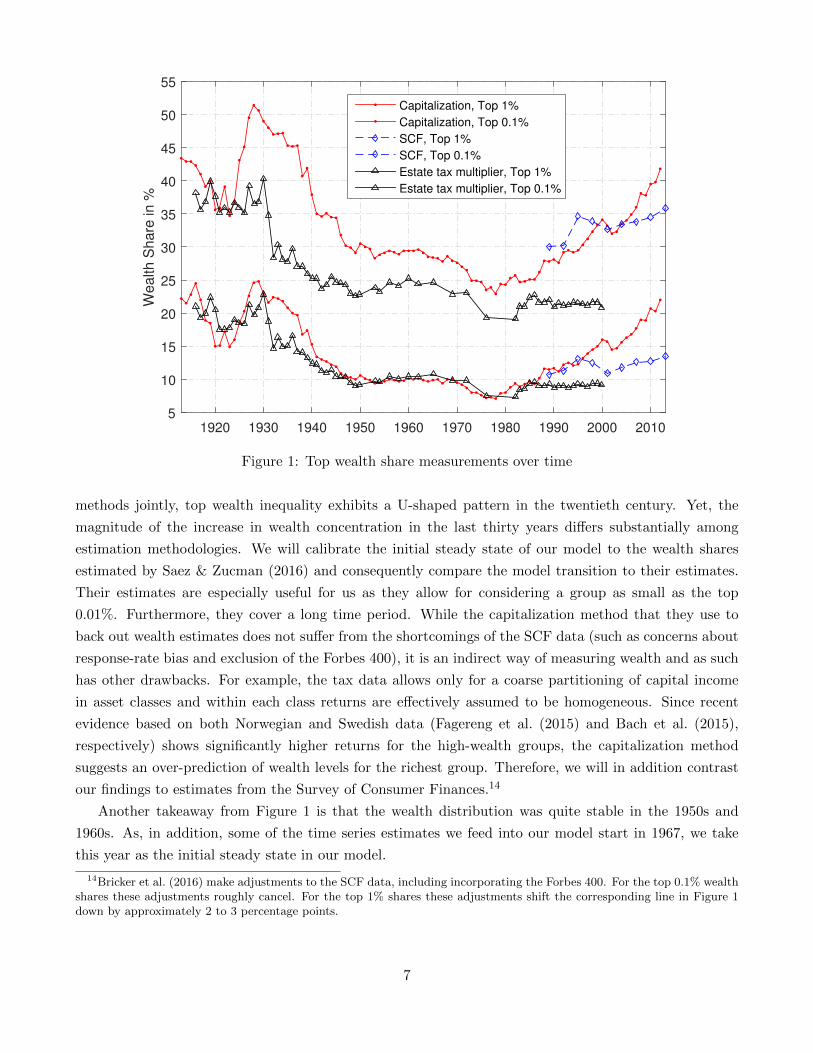
Figure 2 shows the marginal propensity to save out of capital holdings (denoted k in the figure)

arising from the stochastic-β model under study in the present paper.20 As discussed above, the marginal

propensity to save increases in wealth, holding earnings constant, and asymptotes to a constant that

depends on the consumer’s discount factor. Figure 3 displays the tail behavior of the stationary wealth

distribution. In line with the theoretical results in Benhabib et al. (2015b), the logarithm of its counter-

cumulative distribution function becomes linear in the logarithm of assets as assets grow large, indicating

that the right tail of the distribution follows a Pareto distribution.

log(k)2 4 6 8 10 12 14 16

mar

gina

l pro

pens

ity to

sav

e

0.85

0.9

0.95

1

high beta, high earningshigh beta, low earningslow beta, high earningslow beta, low earnings

Figure 2: Asymptotic marginal propensity to save

In light of this result, it is worth noting that the model in Castaneda et al. (2003)—which generates

substantial wealth inequality using an earnings process featuring a low-probability but transient very-

high-earnings state—does not deliver a Pareto tail in wealth. In this model, in which consumers have

a common discount rate, marginal propensities to save do not vary but instead converge to the same

constant, independently of the level of earnings and as a result the steady-state distribution of wealth

does not feature a Pareto tail. This model can deliver such a Pareto tail, however, if the earning process

linearity of the savings rule in a finite-horizon problem as the horizon grows large.20The graphs in this section are derived from a simplified model with a flat tax, to focus on the main mechanism.

11

log(k)-5 0 5 10 15

-18

-16

-14

-12

-10

-8

-6

-4

-2

0

log(Prob(K > k))Top 10%Top 1%Top 0.1%Top 0.01%

Figure 3: Pareto tail of the wealth distribution

itself has a Pareto tail. In the absence of randomness in either discount rates or returns, however,

the wealth distribution inherits not only the Pareto tail of the earnings distribution but also its Pareto

coefficient. Because earnings are considerably less concentrated than wealth, the resulting tail in wealth

is too thin to match the data in such an alternative model.

6 Calibration

In this section, we describe how we calibrate our model economy. As indicated in Figure 1, the U.S.

wealth distribution was roughly stable in the 1950s and 1960s, as was tax progressivity. This, together

with the fact that some of our time series estimates start in 1967, make this year a natural initial steady

state. We set the model period to a year to conform to the tax system.

6.1 Basic parameters

We parameterize the production technology and utility function using standard functional forms and

parameters. The (gross) production function is given by F (K,L) = KαL1−α. The capital share is set

to α = 0.36 and depreciation to δ = 0.048 annually. In an extension (see Section 8.1), we check the

sensitivity of our results to using a constant-elasticity-of-substitution production function with (gross)

elasticity greater than one. The coefficient of relative risk aversion, γ, is set to 1.5.

6.2 The earnings process

The earnings process is based on the traditional log-normal framework with lt(pt, νt) = exp(pt + νt).

That is, we assume that the persistent component pt of the earnings process follows a Gaussian AR(1)

12

1970 1980 1990 2000 20100.1

0.2

0.3

0.4

0.5

0.6Cross-sectional Standard Deviations

persistent componenttransitory component

1970 1980 1990 2000 20101.6

1.8

2

2.2

2.4

2.6

2.8

3Pareto Tail Coefficient Earnings

Figure 4: Earnings process ingredients

process with parameters (ρP , σPt ). The autocorrelation coefficient, ρP , is fixed over time, while the

innovation standard deviation varies. Likewise, the transitory component νt is also assumed to be normally

distributed with standard deviation σTt . We use estimates by Heathcote et al. (2010) that span the period

1967–2000 and assume that the time-varying variances of the innovations are constant thereafter. The

left panel of Figure 4 displays the resulting cross-sectional dispersion. The estimates show a significant

increase in earnings risk for both components.

As is well known, the resulting log-normal cross-sectional distribution of earnings understates the

concentration of top labor income quite severely. Because the observed increase in top labor income

shares is potentially an important explanation for the observed increase in wealth inequality at the top,

we augment the framework for the top 10% earners in such a way that we can directly match the fraction

of labor income going to the top 10%, top 1%, top 0.1% and top 0.01%. In concrete terms, we posit

lt(pt, νt) = ψt(pt) exp(νt), where

ψt(pt) =

exp(pt) if Fpt(pt) ≤ 0.9,

F−1Pareto(κt)

(Fpt (pt)−0.9

1−0.9

)if Fpt(pt) > 0.9.

(7)

Fpt(·) is the cdf of pt and F−1Pareto(κt)(·) the inverse cdf for a Pareto distribution with lower bound F−1pt (0.9)

and shape coefficient κt. Effectively, we thus assume that top earnings are spread out according to a

(scaled) Pareto distribution, while earnings for the majority of workers are distributed according to a log-

normal distribution. The Pareto tail coefficient on labor income κt is then one additional free parameter

to calibrate in each year year. We use estimates on top wage shares from an updated series by Piketty &

Saez (2003) spanning 1967–2011 as calibration targets. The right panel of Figure 4 displays the calibrated

Pareto tail coefficient κt and Figure 5 displays the resulting top labor income shares. That we can match

top labor income shares very well using just a single parameter in each year (i.e., the tail coefficient)

simply reflects the fact that the Pareto distribution is a very good description of the cross-sectional

13

1970 1980 1990 2000 2010

25

30

35

top 10% share

modeldata

1970 1980 1990 2000 2010

6

8

10

12

14top 1% share

1970 1980 1990 2000 2010

1

2

3

4

5

top 0.1% share

1970 1980 1990 2000 2010

0.5

1

1.5

2

top 0.01% share

Figure 5: Top labor income shares in %

earnings distribution at the top.

We do not explicitly model unemployment, nor voluntary non-employment or retirement. We do,

however, introduce a zero-earnings state, occurring with probability χ0 = 0.075 independently of (pt, νt)

and over time, reflecting both long-term unemployment and shocks that trigger temporary exit from the

labor force. This probability is calibrated, together with a borrowing constraint amounting to roughly

one yearly lump-sum transfer, so that the initial steady-state wealth distribution matches both the share

of wealth held by the bottom 50% and the fraction of the population with negative net wealth.

6.3 Tax system

The progressivity of the U.S. tax system has decreased substantially over the model period. To account

for these changes, we use estimates on federal effective tax rates by Piketty & Saez (2007) for the period

1967–2000, keeping them constant thereafter. These comprise the four major federal taxes: individual

income, corporate income, estate and gift, and payroll taxes.21 Piketty & Saez (2007) calculate effective

average tax rates for eleven income brackets, with a particularly detailed decomposition for top income

21Given that our model abstracts from the life cycle, it is appropriate to include the estate tax in the tax on total income,thus effectively smoothing out the incidence of this tax over the life cycle. Ignoring the estate tax would mean omitting amajor source of decreasing tax progressivity. Piketty & Saez (2007) assume further that the corporate income tax burden fallsentirely (and uniformly) on capital income. They argue that this is a middle-ground assumption (regarding the resulting taxprogressivity) between assuming that the tax falls solely on shareholders at one extreme and assuming that it is effectivelyborn by labor income at the other extreme.

14

1970 1975 1980 1985 1990 1995 20000.1

0.2

0.3

0.4

0.5

0.6

0.7

0.8

top rate5 * average income3 * average incomeaverage income

Figure 6: Imputed marginal tax rates for selected total income levels

groups (up to the top 0.01%). We translate this data to our model by means of a step-wise tax function

τt(·) with eleven steps. For each bracket, the threshold is set to match its income share in the data and

the marginal tax rate such that the resulting average tax rate aligns with the data. Figure 6 shows that

the U.S. tax system has indeed become much less progressive over the model period.

Note that in our model taxes τt(yt) are a function of total income yt, consistent with the measurement.

A weakness of our calibration is that we do not have separate tax rates for different sources of income,

but a strength is that we use effective tax rates, thereby accounting for tax avoidance and changing

portfolio composition to the extent that these vary systematically with income. To account for government

transfers, we introduce a social safety net in the simplest possible way by assuming that each agent

receives an (untaxed) lump-sum transfer Tt every period, its size being a constant fraction λ = 0.6 of tax

revenues.22

Note that the income tax does not distort labor supply in our setting, since we assume the latter is

exogenous. This simplification is obviously not a good one for understanding the welfare consequences of

changes in tax rates, but because our current focus is on wealth accumulation and its distribution in the

population we do not think that it is a major shortcoming.

6.4 Idiosyncratic discount rates and returns to capital

Finally, we calibrate the processes for the discount factor (β) and for the returns to capital (η)to match the

right tail of the wealth distribution in the initial steady state. Intuitively, the discount-factor distribution

22About 60% of total federal outlays are mandatory spending, the bulk of it on Social Security, Medicare, Medicaid, andincome security programs (CBO, 2015). The remainder is spent on the Department of Defense and other government agenciesas well as on interest payments.

15

affects the entire asset distribution. In terms of effects on the right tail of the distribution, both discount-

factor and return heterogeneity are crucial and, as discussed in 5 above, they influence its Pareto tail

coefficient. Return heterogeneity does not play a crucial role for the left tail of the wealth distribution

where assets are essentially zero.

To explain how we discipline our parameter selection based on the data at hand, note first that

variation in either β or η generates right-tail wealth inequality. Second, persistence in these parameters is

a particularly powerful force toward dispersion. Ideally, one would estimate the entire η distribution based

on individual panel data on asset returns, and one would want to also use panel data on saving rates.

Since we do not have U.S. data of this sort we did not follow this route in this paper, but we are hopeful to

follow this strategy in future work. We do motivate our assumptions here based on the two papers using

Norwegian and Swedish data cited above (Fagereng et al. (2015) and Bach et al. (2015), respectively),

which both strongly argue that there is a significant idiosyncratic returns component. These papers also

argue that there is persistence in returns but their interpretations of this finding differ. The possibility

that different households have different skills at return finding (an interpretation made in Fagereng et al.

(2015)) is radical relative to the finance literature, and although we do not want to rule out that this

hypothesis is true, we opted for the more conservative assumption that idiosyncratic return differences

are iid, while allowing persistence in βs.

We use an AR(1) structure for the discount factor. Thus, from the perspective of dispersion we

have three key parameters to calibrate: the variance and persistence of β and the variance of η. First,

we follow in selecting the persistence of the β process based on what seems a priori reasonable given a

generational structure. Second, we target two wealth-distribution statistics to obtain the remaining two

variance elements (for β and η): the Pareto tail coefficient and the fraction of total wealth held by the

10% richest. This identifies our parameters. We now describe the details.

We posit that β follows a Gaussian AR(1) process:

βt = ρββt−1 + (1− ρβ)µβ + σβεβt , εβt ∼ N(0, 1).

Moreover, we assume that the idiosyncratic factor in the return to capital is normally distributed: ηt ∼i.i.d.

N(1, ση). Importantly, all these parameters are fixed over time (by varying them freely we could of course

track the evolution of the wealth distribution more or less exactly). The mean discount factor determines

the equilibrium capital-output ratio and we set it to µβ = 0.92 to match a ratio of capital to net output of

about 4 in the initial steady state. The calibrated stochastic-β parameters are ρβ = 0.992 and σβ = 0.0019,

implying that the standard deviation of the cross-sectional distribution of discount factors, which does not

vary over time, is 0.0148. Moreover, the choice of ρβ implies that roughly one third of the gap between a

given discount factor and the average discount factor is closed within a generation. The idiosyncratic noise

in the return to capital is set to equal ση = 0.725, implying that the gross (pre-tax, net of depreciation)

return on capital (1 + r?η) lies in the interval [0.9874, 1.1437] for 90% of all agents in the initial steady

state. Interestingly, although these parameters were selected based on the procedure outlined above, the

implied idiosyncratic variation of returns in our calibration turns out to be close to the amount found by

Fagereng et al. (2015) in Norwegian data; see, for example, Panel C of Table 1 in that paper. Bach et al.

16

Table 1: Matching the 1967 wealth distribution as a steady state

Parameter ρβ σβ ση a χ0

Value 0.992 0.0019 0.725 −0.24 0.075

Target Top 10% share Top 1% Top 0.1% Top 0.01% Bottom 50% Fraction a < 0

Data 70.8% 27.8% 9.4% 3.1% 4.0% 8.0%Model 70.6% 28.1% 9.5% 2.9% 3.1% 7.0%

(2015), moreover, find roughly comparable amounts of variation in Swedish data.

To summarize, Table 6.4 lists the values of the five parameters (persistence and standard deviation

of the discount rates; standard deviation of return shocks; the borrowing constraint; and the probability

of zero income) calibrated to match as closely as possible six features of the initial steady-state wealth

distribution: the shares held by the top 10%, the top 1%, the top 0.1%, the top 0.01%, and the bottom

50% as well as the fraction of the population with negative net wealth. The fit is excellent at both ends

of the distribution.23 To the extent that the right tail of the wealth distribution has a Pareto tail, we are

therefore also matching the Pareto coefficient governing its thickness, because this coefficient is pinned

down by the ratio of the top 0.01% share to the top 0.1% share, or the ratio of the top 0.1% share to the

top 1% share, both of which are roughly one-third, both in the model and in the data.

Two comments are in order. First, when solving the model numerically we truncate the β and η

distributions to ensure that the consumer’s optimization problem is well-defined (with finite present-value

utility) and that a stationary distribution of wealth emerges. Unlike in a standard Aiyagari economy

without heterogeneity in preferences, in our model some agents temporarily have discount rates that are

smaller than the rate of return, a necessary condition for generating a Pareto tail in the wealth distribution

(see the discussion in Section 5). It follows that the support of the stationary wealth distribution is not

bounded from above. In practice, we use a large enough upper bound in our numerical implementation

so that the resulting truncation error is negligible.24

Second, if our goal were solely to match the Pareto coefficient in the right tail of the wealth distribution,

it would be excessive to calibrate as many as five parameters to match features of the wealth distribution.

But the tail coefficient is not a sufficient statistic for wealth inequality unless the entire distribution is

(counterfactually) Pareto-shaped: even if, say, the top 1% of the wealth distribution can be described

exactly by a Pareto distribution, the tail coefficient determines only the distribution of wealth within these

top 1% but not the fraction of total wealth held by the top 1%. While stochastic discount factors are the

main force driving the shape of the upper tail in the initial steady-state wealth distribution, to achieve

our objective of replicating the distribution of wealth on its entire domain we found that introducing in

addition a reasonable amount of randomness in returns helped to improve the fit. Moreover, because

ownership of primary residences and poorly diversified private equity account for a sizable fraction of net

23The data on top wealth shares in Table 6.4 is from Saez & Zucman (2016), who use a capitalization method to calculatethem. Because this method is unreliable for a breakdown of the bottom 90%, the other data moments are based on surveydata (SCF and precursors); see Kennickell (2011).

24Appendix A describes in detail our numerical procedure.

17

wealth, we view randomness in returns as a realistic feature of individual asset accumulation.25

7 Results

In Section 6, we showed that our model framework, when properly calibrated, can replicate wealth het-

erogeneity, including the Pareto-shaped right tail, as well as other macroeconomic moments in the initial

steady state. We proceed in this section to report on our main result: the evolution of the wealth dis-

tribution in the our model economy contrasted with the data. Subsequently, we employ counterfactual

analysis in order to decompose those overall changes and identify the key drivers of movements in the

wealth distribution.

7.1 Benchmark transition experiment

We summarize the findings from our main experiment in a set of tables: Tables 2-5. The tables differ

in terms of the moments of the data we look at and the particular data set we compare the model to;

the use of different tables is motivated by different coverage of the different data sets and should help

readability.26

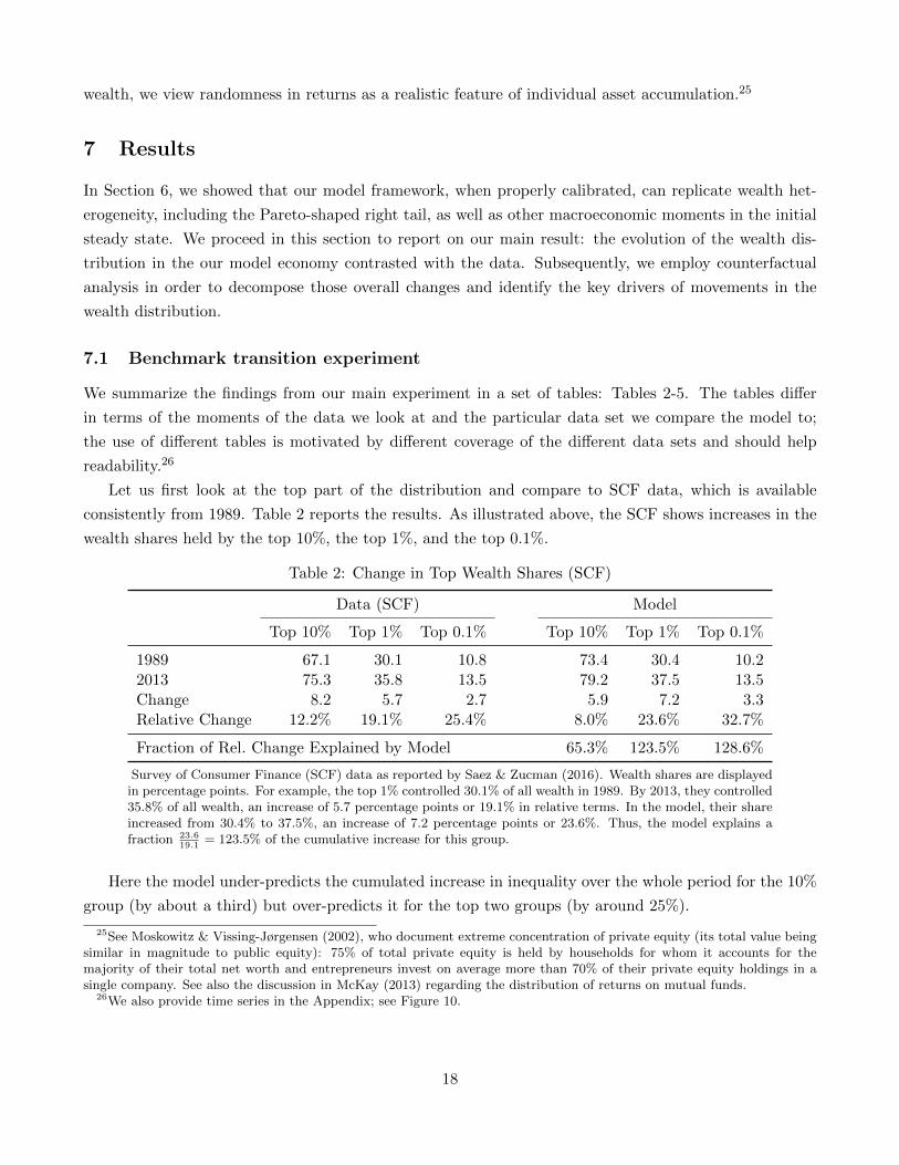
Let us first look at the top part of the distribution and compare to SCF data, which is available

consistently from 1989. Table 2 reports the results. As illustrated above, the SCF shows increases in the

wealth shares held by the top 10%, the top 1%, and the top 0.1%.

Table 2: Change in Top Wealth Shares (SCF)

Data (SCF) Model

Top 10% Top 1% Top 0.1% Top 10% Top 1% Top 0.1%

1989 67.1 30.1 10.8 73.4 30.4 10.22013 75.3 35.8 13.5 79.2 37.5 13.5Change 8.2 5.7 2.7 5.9 7.2 3.3Relative Change 12.2% 19.1% 25.4% 8.0% 23.6% 32.7%

Fraction of Rel. Change Explained by Model 65.3% 123.5% 128.6%

Survey of Consumer Finance (SCF) data as reported by Saez & Zucman (2016). Wealth shares are displayedin percentage points. For example, the top 1% controlled 30.1% of all wealth in 1989. By 2013, they controlled35.8% of all wealth, an increase of 5.7 percentage points or 19.1% in relative terms. In the model, their shareincreased from 30.4% to 37.5%, an increase of 7.2 percentage points or 23.6%. Thus, the model explains afraction 23.6

19.1= 123.5% of the cumulative increase for this group.

Here the model under-predicts the cumulated increase in inequality over the whole period for the 10%

group (by about a third) but over-predicts it for the top two groups (by around 25%).

25See Moskowitz & Vissing-Jørgensen (2002), who document extreme concentration of private equity (its total value beingsimilar in magnitude to public equity): 75% of total private equity is held by households for whom it accounts for themajority of their total net worth and entrepreneurs invest on average more than 70% of their private equity holdings in asingle company. See also the discussion in McKay (2013) regarding the distribution of returns on mutual funds.

26We also provide time series in the Appendix; see Figure 10.

18

Looking at the same population percentiles and comparing the model data to the Saez & Zucman

data, we can now go back and cumulate wealth increases from 1967. Table 3 gives the key numbers.

Table 3: Change in Top Wealth Shares (Saez & Zucman)

Data (Saez & Zucman) Model

Top 10% Top 1% Top 0.1% Top 10% Top 1% Top 0.1%

1967 70.8 27.8 9.4 70.6 28.1 9.52012 77.2 41.8 22.0 79.0 37.3 13.4Change 6.4 14.0 12.6 8.4 9.2 3.9Relative Change 9.0% 50.4% 134.0% 11.9% 32.5% 41.0%

Fraction of Rel. Change Explained by Model 132.2% 64.6% 30.6%

Data based on the capitalization method estimates by Saez & Zucman (2016).

Here the model over-predicts the increase in the fraction of wealth held by the top 10% by about

one third, whereas it under-predicts the increases for the two top groups, by about one and two thirds,

respectively. Clearly, in terms of the model’s relative performance across groups, the two data sets give

different answers, but it is comforting that the under- or over-predictions of the model are not systematic

across data series. In terms of shorter-run dynamics, wealth inequality in the Saez & Zucman data set

shows a U-shaped pattern within the period, with a trough in the late 1970s. The model’s dynamics

deliver a U-shaped pattern in growth rates but not in levels; we will discuss the shorter-run aspects of

the model-data comparison in more detail in Section 8.3 below.

The results for the bottom 50% of the population, where we do have a consistent data series from the

SCF beginning in 1967, are contained in Table 4.27 The bottom 50% have lost a little over two thirds;

the model accounts for about two thirds of this decline in wealth.

Table 4: Change in Bottom 50% Wealth Share

Data (SCF) Model

1967 4.0* 3.12010 1.1 1.4Change -2.9 -1.7Relative Change -72.5% -55.3%

Fraction Explained 76.2%

* Data point equals the median of estimates based on SCFprecursors in the 1960s, as reported by Kennickell (2011).

Finally, looking at the very richest, and here only Saez & Zucman have data, we see in Table 5 that

the model’s performance is still qualitatively correct but now the quantitative under-prediction is more

sizable.

The model predicts an increase in the fraction of wealth held by the top 0.01% by about a half,

whereas in the Saez & Zucman data set the increase is fivefold. Clearly, although—as suggested above—

27The method of Saez & Zucman’s unfortunately does not allow for a breakdown of the bottom 90% into subgroups.

19

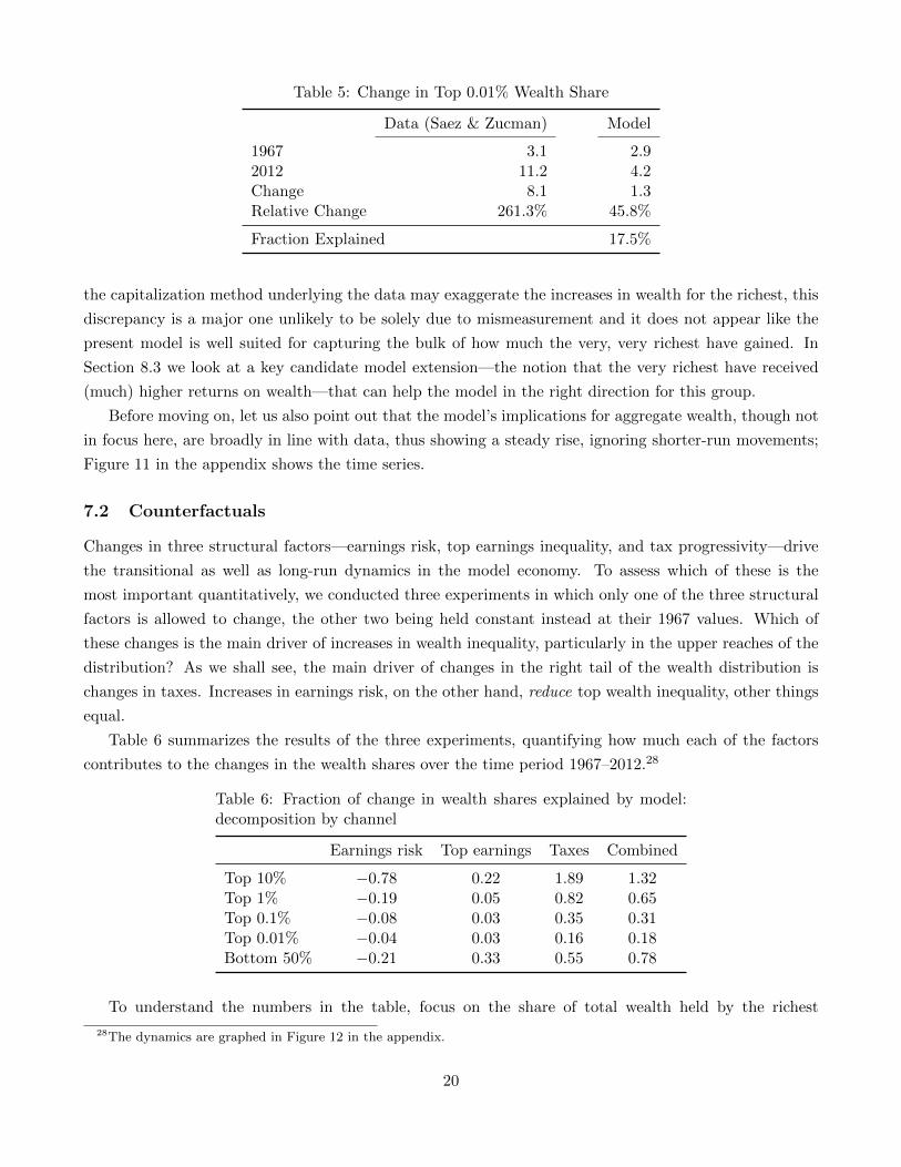
Table 5: Change in Top 0.01% Wealth Share

Data (Saez & Zucman) Model

1967 3.1 2.92012 11.2 4.2Change 8.1 1.3Relative Change 261.3% 45.8%

Fraction Explained 17.5%

the capitalization method underlying the data may exaggerate the increases in wealth for the richest, this

discrepancy is a major one unlikely to be solely due to mismeasurement and it does not appear like the

present model is well suited for capturing the bulk of how much the very, very richest have gained. In

Section 8.3 we look at a key candidate model extension—the notion that the very richest have received

(much) higher returns on wealth—that can help the model in the right direction for this group.

Before moving on, let us also point out that the model’s implications for aggregate wealth, though not

in focus here, are broadly in line with data, thus showing a steady rise, ignoring shorter-run movements;

Figure 11 in the appendix shows the time series.

7.2 Counterfactuals

Changes in three structural factors—earnings risk, top earnings inequality, and tax progressivity—drive

the transitional as well as long-run dynamics in the model economy. To assess which of these is the

most important quantitatively, we conducted three experiments in which only one of the three structural

factors is allowed to change, the other two being held constant instead at their 1967 values. Which of

these changes is the main driver of increases in wealth inequality, particularly in the upper reaches of the

distribution? As we shall see, the main driver of changes in the right tail of the wealth distribution is

changes in taxes. Increases in earnings risk, on the other hand, reduce top wealth inequality, other things

equal.

Table 6 summarizes the results of the three experiments, quantifying how much each of the factors

contributes to the changes in the wealth shares over the time period 1967–2012.28

Table 6: Fraction of change in wealth shares explained by model:decomposition by channel

Earnings risk Top earnings Taxes Combined

Top 10% −0.78 0.22 1.89 1.32Top 1% −0.19 0.05 0.82 0.65Top 0.1% −0.08 0.03 0.35 0.31Top 0.01% −0.04 0.03 0.16 0.18Bottom 50% −0.21 0.33 0.55 0.78

To understand the numbers in the table, focus on the share of total wealth held by the richest

28The dynamics are graphed in Figure 12 in the appendix.

20

percentile. Saez & Zucman (2016) measure an increase in this share from 27.8% to 41.8% from 1967

to 2012. Over the same time period, allowing for changes only in earnings risk and keeping all other

parameters fixed at their initial steady-state values, the model predicts a decrease from 28.0% to 25.2%.

Changes in earnings risk therefore explain a fraction 25.2−28.028.0 /41.8−27.827.8 = −0.19 of the actual change.29

Again, the observed increases in earnings risk reduce inequality, moving it in the opposite direction from

the observed changes! (Separate increases in either the persistent or transitory components of earnings

risk also reduce inequality.) Instead, as can be seen for all the different distributional statistics, the main

driver of the surge in wealth concentration is the changing U.S. tax system. The increase in top earnings

inequality (parameterized by changes over time in the the Pareto tail coefficient κt on labor income) has

worked in the same direction, although the effect of this channel is much smaller.

Why does an increase in earnings risk reduce wealth inequality? As noted in Section 1, persistent

heterogeneity in discount rates is a powerful force driving the wealth distribution apart: with permanently

different discount rates and complete markets against earnings risk, the most patient would eventually

hold all the economy’s wealth.30 Earnings risk, then, is a friction, or glue, that keeps the distribution from

flying apart altogether as in Becker (1980)’s work cited in Section 1. This risk operates especially strongly

at the low end of the wealth distribution, where poorer consumers save to move away from borrowing

constraints when earnings risk is larger.

In our model higher earnings risk also generates a thinner right tail in the wealth distribution because

the resulting increase in aggregate precautionary savings drives down the equilibrium interest rate. This

drop in the interest rate shifts the distribution of savings propensities to the left, particularly for the well-

insured wealthy consumers for whom wage risk is largely immaterial and who therefore have essentially

linear decision rules. As discussed in Section 5, the Pareto tail coefficient, ζ, is defined implicitly by the

equation E[sζ ] = 1, where s is the (asymptotic) marginal propensity to save out of wealth. As s falls for

all discount-factor types, ζ must increase to compensate, i.e., the Pareto tail becomes thinner.31

Why have changes in the tax system induced such large changes in wealth inequality? Note first

that the average tax rate (i.e., total tax revenues as a fraction of net GDP) in our model increases from

0.23 to 0.27 over the period 1967–2012. An increase in average taxes tends to reduce effective earnings

risk (because the tax is multiplicative), increasing inequality for the same reason (but in the opposite

direction) that the observed increases in (pre-tax) earnings risk reduce inequality. This effect, however,

is a small one unless the average tax rate changes dramatically. Much more important quantitatively

is the dramatic decrease in tax progressivity, where even small changes have large effects on inequality,

especially at the high end of the wealth distribution. There are both partial- and general-equilibrium

effects at work here. Starting with the latter, it is well known in the context of complete-markets models

without discount-factor or wage heterogeneity that progressivity in the tax rate on saving is a strong

force toward long-run equality, whereas mere proportional taxes are consistent with any distribution of

29Note that the fractions generally do not add up to the fraction explained when feeding in all observed changes at thesame time, as in our benchmark experiment. The remainder is due to interaction effects in general equilibrium.

30In our model, idiosyncratic returns are statistically independent across time, but were they persistent they would actmuch like persistent heterogeneity in discount rates to spread out the wealth distribution, because discount rates and returnsenter similarly in consumers’ Euler equations.

31Nirei & Aoki (2016) observe the same effect.

21

wealth as a steady-state equilibrium.32 The mathematical intuition behind the force of progressivity is

particularly clear in a simple case where the marginal tax rate is strictly increasing in wealth. Here,

because all consumers face the same market rate under complete markets (and have the same discount

rates and wage incomes), they also need to have the same net of tax return if their consumption levels

are all constant (or growing at a common constant rate); hence they need to have the same wealth in

the long run. This mechanism is still present in a more general model such as the present one, which has

incomplete markets and differences in wages and discount rates, though with less long-run poignancy: a

strictly increasing marginal tax rate is still consistent with long-run wealth inequality.

Turning to the partial equilibrium analysis, which influences the transition path too, note that the

marginal saving propensity (out of initial-period assets) for a well-insured consumer with power utility is

approximately β(1 + r(1− τ ′(y))) raised to a positive power, where β is the consumer’s current discount

factor and τ ′(y) is the consumer’s current marginal tax rate.33 This tax rate varies with the consumer’s

income, y, but it is persistent over time because income is persistent. Tax progressivity, therefore, gen-

erates persistent differences across consumers that act like persistent differences either in the consumers’

after-tax rates-of-return, r(1− τ ′(y)), or, equivalently, in consumers’ discount factors. Consequently, de-

creases in progressivity have the same effect as increasing the spread of discount factors, a powerful force

for generating differential savings behavior and as a result higher wealth inequality. In Figure 14 in the

appendix we break down the effects of progressivity into a direct effect—the return differences implied by

changed progressivity—and that on behavior—marginal saving propensities excluding the return effect—

by showing the effects of the latter only and the effects of the former only, along with the full equilibrium

response. Clearly, the former is most important for the very richest and hence for changes in top wealth

inequality.

In sum, among the different drivers of wealth inequality considered in the benchmark experiment it

is clear that decreasing tax progressivity is key: it spreads out the resources available to consume and

invest and it increases the relative return of the rich on any given saving.

In a representative-agent model the increase in average taxes would lead in equilibrium to a decrease

in the capital-to-output ratio, but it does not in our heterogeneous-agent model for three reasons. First,

the (smallish) increase in average taxes does not offset the even larger increase in the riskiness of pre-tax

earnings, leading to more precautionary savings in the aggregate. Second, decreasing tax progressivity

increases the returns to saving, a particularly powerful force for the rich. Third, the increasingly “thick”

right tail in earnings provides the rich (who tend to be those with high earnings) with additional resources

for saving. These three forces combine to generate a fairly large increase in the ratio of capital to net

output over the period 1967–2012.

Finally, if one looks at the wealth holdings of the bottom 50% of the population, the bulk of the

decrease is again accounted for by the decrease in tax progressivity, while the movements in the aggregate

capital-output ratio are mostly accounted for by the increase in earnings risk.34

32Total wealth is of course pinned down so that the return to saving equal the discount rate, abstracting from consumptiongrowth.

33With u(c) = c1−σ−11−σ , the power is 1/σ.

34Figure 13 in the appendix displays these results.

22

8 Extensions

We now visit a number of robustness exercises and extensions. First, we look at an aggregate production

function with a non-unitary elasticity of substitution between capital and labor; our benchmark Cobb-

Douglas (the unitary case) function does take a particular stand on the dynamics of the returns to capital.

We find that this mechanisms does not appear very promising for understanding the data at hand.

We then weaken the consumers’ ability to predict changes in their environment. In particular, in

our benchmark experiment we assume that consumers in 1967 could predict the future paths of the tax

schedule and the degree of idiosyncratic risk, arguably a very strong assumption, so it is interesting to

compare this case to one with more limited abilities to predict. Here, our finding is that a model with

entirely myopic expectations (the current policy/risk environment is expected to last forever) behaves

almost like our benchmark environment.

The benchmark experiment in our paper emphasized the secular changes in inequality over the sample

period, i.e., the cumulative increases in the wealth fractions attributable to the richest percentiles of the

population. We found that the model could account for a significant share of the observed changes (and

that the discrepancies depend on which data one compares to) and that the key factor was the decrease

in tax progressivity that began in the late 1970s. At the same time, as we pointed out but did not focus

on, the model does not do as well in replicating some of the shorter-run movements in inequality. In

particular, in the Saez & Zucman data set (see Figure 1), there is a fall in inequality from 1967 to just

before 1980 and since then an increase. This U shape is not captured by our model: the model has a

kink, but in the growth rate of inequality (an initial near-zero rate and a later significant positive rate).

To examine further mechanisms behind a possible U shape, we consider rate of return variation driven

by two factors: inflation (which has an effect via progressivity) and stock-market valuation (where richer

households benefit more from market increases since they hold more risky assets). These two mechanisms

are harder to embed in a choice framework, let alone one with a general equilibrium, and our extension here

is therefore a first pass where we use partial-equilibrium analysis and hard-wired differences in portfolio

choice between rich and poor households. We find that the valuation channel holds important promise for

understanding the dynamics of inequality but that the inflation channel appears to be of second order,

despite the large movements in inflation during the period.

8.1 Robustness to the elasticity of substitution in production

The stability of the fraction of income accruing to labor, for a long time a central pillar of macroeconomic

models, has recently been questioned. Karabarbounis & Neiman (2014b), among others, document a

visible (though not large) decline in the labor share. Using a production function with a constant elasticity

of substitution (CES), they estimate an elasticity of substitution between capital and labor of 1.25. To

look into the possibility of a falling labor share, we use a standard CES production function,

FCES(Kt, L) = ACES

(αCESK

σ−1σ

t + (1− αCES)Lσ−1σ

) σσ−1

, (8)

23

where ACES and αCES are chosen such that the initial steady state is identical to the Cobb-Douglas

benchmark. Over time, there is capital deepening, leading to a lower labor share because the elasticity of

substitution is above one. We find, however, only very small differences as compared to the Cobb-Douglas

benchmark (see Table 7).35

Table 7: Robustness to the input substitution elasticity and to myopia

Top 10% Top 1% Top 0.1% Top 0.01% Bottom 50% KY r

1967 70.6 28.1 9.5 2.9 3.1 3.74 6.56

2012Benchmark 79.0 37.3 13.4 4.2 1.3 4.24 5.41CES 78.7 36.9 13.2 4.1 1.4 4.28 5.57Myopia 77.1 36.3 13.3 4.2 1.6 4.21 5.47

Wealth shares and the interest rate r are reported in %. This table compares various statistics from the benchmarkmodel transition to alternatives. In the benchmark transition experiment, the production technology is assumed tobe Cobb-Douglas and agents have perfect foresight. The row labeled ’CES’ reports results from a model with CESproduction technology. The row labeled ’Myopia’ reports results from a transition experiment in which agents arecompletely myopic about the future, assuming present prices, as well as the parameters of the earnings processand the tax schedule, will prevail.

Capital deepening leads to a smaller reaction of the interest rate, so the rise in the capital-output ratio

is slightly larger in equilibrium and the Gini coefficient on gross income increases a small amount more

(relative to the benchmark).36 At the same time, we find that top wealth shares increase more slowly;

unlike for the decline in tax progressivity, higher equilibrium interest rates induce more savings across the

whole wealth distribution. In other words, at least over the time frame considered, the saving of the poor

tends to be more elastic with respect to the interest rate than the saving of the rich. Overall, though, the

message here is that the quantitative effects of considering a different elasticity of substitution are very

small.

8.2 Robustness to agents’ abilities to predict policy and risk

It is surely bold to assume that agents have perfect foresight on the entire path of the tax schedule, the

parameters governing the earnings process, and the resulting equilibrium prices. To gauge the sensitivity

of our findings to this assumption, we computed the transitional dynamics under complete myopia, i.e.,

a polar opposite case in terms of agents’ ability to predict. That is, in every period agents believe that

the current environment will prevail forever and, accordingly, they are surprised to learn about their

forecasting mistake in the subsequent period.37 Table 7 shows the effects of myopia in the last row.38

Clearly, the differences are very small. We conclude that the perfect-foresight assumption is not critically

driving the results in the benchmark experiment.

35Figure 15 in the appendix shows the time series.36In addition, the gross labor share falls by about one percentage point over the period 1967–2012 in our model, though

the net labor share actually rises a little. Karabarbounis & Neiman (2014a) report that since 1975 the gross labor share inthe U.S. has fallen by about five percentage points and the net labor share by about two-and-a-half.

37See Section 4.2 for an exact description of how this experiment is conducted.38Figure 16 in the appendix shows the time series.

24

8.3 Changes in returns: a preliminary look at valuation and inflation effects

In this section we look at the possibility that returns on saving differ systematically across wealth groups,

as indicated in Bach et al. (2015) and Fagereng et al. (2015) as well as via the the fact that the tax

schedule is progressive and not inflation-indexed. As for the former effect, there seems to be some extent

of “increasing returns” to wealth accumulation. The modeling in this section will be based on partial

equilibrium and hard-wiring of the features observed in data, and thus the results here should be viewed

as providing some directions for potential future work. We first briefly discuss why a full treatment is

beyond the scope of the present paper.

First, heterogeneity in the returns to saving is incorporated in the benchmark model but in the form

of hard-wired idiosyncratic differences unrelated to wealth (this feature was found to be important for

matching the initial wealth distribution). It is challenging to go beyond the hard-wiring of portfolio

choice. One could try to square differences in idiosyncratic returns and rational decision making (i.e.,

why more diversification is not chosen) by explicitly modeling asymmetric information, but to provide a

quantitative version of such a theory would amount to a whole project in itself.

Second, as for allowing different portfolios in terms of aggregate returns (nominal vs. real assets,

risky vs. risk-less assets), it is arguably equally challenging to provide a quantitative theory based on full

portfolio choice. Under some conditions, the more well-insured are consumers to idiosyncratic shocks, the

higher a portfolio share will they invest in risky assets. However, the benchmark model displays little

sensitivity to risk, for reasons rooted in the causes of the equity premium puzzle. That is, consumers

mostly care about returns and not about risk, so that the portfolio choices will be virtually the same

across different levels of wealth.39

Third, to provide a general-equilibrium theory one would need to derive return differences that are of

the magnitude observed—the equity premium puzzle. There are ways to accomplish this and they rely on

considering different consumer preferences (possibly in combination with different assumptions on returns,

such as low-probability disaster outcomes or long-run risk components). Such preferences (with habits or

non-additivity), however, have not been explored much in terms of their cross-sectional implications and

thus one would need to consider a different benchmark model altogether. This is an interesting project in

itself but it is also beyond the scope of the present paper. Relatedly, there are ways to computationally

handle the incorporation of aggregate risk (e.g., Krusell & Smith (1998)) but to deal with aggregate risk,

portfolio choice, and a nontrivial dynamic transition path is really at the frontier of our computational

abilities.40

Fourth, in reality there is also a choice between nominal and real assets and any inflation-based

arguments for differences in returns would need to explain what mixes of real and nominal assets are held

at different wealth levels.

For these reasons, in this section we simply assume systematic wealth-related differences in portfolio

choice and we assume that the returns to risky and risk-less assets are exogenous; for the inflation

39This point is made in detail, and a full portfolio-choice model is solved, in Krusell & Smith (1997).40Methods based on linearization with respect to aggregates, such as those in Reiter (2009) or, more recently, Ahn et al.

(2017), cannot be used since they imply certainty equivalence.

25

experiment we simply assume that all assets are nominal.

8.3.1 Valuation effects

We thus take the dynamic path of the real interest rate as given from the benchmark transitional experi-

ment, and we also use the equilibrium wages, transfers, and the decision rules. That is, we are given how

much people save in this equilibrium at each moment in time and for each outcome of their individual

states and we then simply append a return composition to this level of saving. To implement this, we

use portfolio weights (for risky and risk-less assets) from Bach et al. (2015), which offers direct data on

portfolios.41 These patterns are summarized in Figure 7.

00.10.20.30.40.50.60.70.80.91

RiskyAssetPortfolioWeights

Figure 7: Portfolio Weights

We then use the U.S. time series on stock market returns (using the S&P and including dividends in

the returns) and fluctuations in the short-run real interest rate to generate the return outcomes. These

are displayed in Figure 8.

1970 1975 1980 1985 1990 1995 2000 2005 2010-40

-30

-20

-10

0

10

20

30

40

An

nu

al R

etu

rn in

%

Riskfree Real Interest Rate

Real S&P Return

Equity Premium

Figure 8: Annual Real Interest Rate and Real S&P Return

We now interpret the portfolios of the initial steady state as having reflected both a riskless and a

risky part with the associated return differences taken as an average from the pre-1967 period and we

41Using the portfolio weights found by Fagereng et al. (2015) yields similar results.

26

assume a flat capital-gains tax on the risky part of the portfolio following the historical evolution of this

tax; the details of the computations are contained in Appendix C.

The results on wealth shares from the valuation experiment are displayed in Table 8; Figure 17 in the

appendix shows the time series. The table has two parts: on the left-hand side, we see the initial decrease

in inequality (a negative entry indicates a decrease throughout the table) and on the right-hand side the

cumulative over the whole period. The valuation effects are tabulated in the third row.

Table 8: Valuation and Inflation Effects

Initial-to-Trough Cumulative

Top 10% Top 1% Top 0.1% Top 10% Top 1% Top 0.1%

Data (Saez & Zucman) -7.2 -4.9 -2.3 6.4 14.0 12.6Benchmark Model (BM) 0.0 0.0 -0.1 8.4 9.2 3.9BM + Valuation Effects -6.9 -5.4 -2.5 3.8 4.0 1.7BM + Inflation -2.5 -3.2 -1.6 5.1 5.5 2.6

This table reports changes in wealth shares in percentage points. The columns titled ‘Initial-to-Trough’ refer tothe change in the share of wealth held by a particular group from the start of the time series in 1967 to its trough(which is around 1980). The columns titled ‘Cumulative’ refer to the cumulative change from 1967 to 2012. Thedata is from Saez & Zucman (2016). The second line reports wealth shares from the benchmark model transition.The third line reports shares from an out-of-equilibrium experiment that adds valuation effects to the benchmarkmodel. The shares in the last row refer to a similar experiment that incorporates the interaction between inflationand the tax code in the benchmark model.

Looking at the cumulative effects first, there are visible effects of portfolio differences across wealth

groups on inequality over the period: because the equity premium over the period has been somewhat

lower than prior to 1967, inequality goes up a few percentage points less than in the benchmark model.

More interestingly, however, the dynamics within the period are strongly accentuated due to valuation

movements. From 1967 to 1980, when the trough is reached, the inclusion of valuation effects induces

changes in the top shares that are very similar to those in the data for top 10%, top 1%, and top 0.1%. For

the extreme right tail (0.01%) of the wealth distribution, the valuation effects do not suffice in generating

the large recent run-up in wealth, but it is highly likely that valuation effects can play a role here too,

though through various forms of private equity not captured by a broad stock index. We conclude that

in order to understand shorter-run movements in the data, valuation effects seem quite promising. Given

their importance in accounting for relative wealth shares, moreover, it becomes all the more urgent to

explore different theories for their behavioral underpinnings in future work.

8.3.2 Inflation

As background for the table, the derivations in the appendix, Section D, show how progressivity interacts

with inflation to lower the relative returns on saving as a function of wealth. The data in Figure 9 shows

the rather dramatic movements in inflation over the period.

Turning to the results of these effects over the given period, Table 8 shows the results for inflation in

the last row; Figure 18 in the appendix shows the time series. The effects of inflation are similar to those

arising from valuation changes, though weaker. There are some cumulative effects, also lowering wealth

27

1970 1975 1980 1985 1990 1995 2000 2005 2010 2015

0

2

4

6

8

10

12

14

Infla

tio

n R

ate

in

%

Annual Inflation Rate (CPI)

1967 Steady State Inflation

Figure 9: Annual Inflation Rate (CPI)

inequality somewhat relative to the benchmark. Second, the movements in inflation also help generate

a U-shaped pattern in the wealth shares of the richest. To understand these findings, note that over

the period up to around 1980, there was an upward drift in inflation and progressivity remained at a

high level, thus accounting for a downward movement in the wealth shares of the richest. The Volcker

disinflation era that followed then amounted to a positive effect on the shares of the richest, though these

effects were limited by the fact that progressivity also fell—progressivity is a necessary component of

inflation effects.42 Going forward, unless both inflation and progressivity rises, inflation will not likely be

a major contributor to changes in the wealth shares across the population.

8.4 The long run

We have focused so far on the transitional dynamics of the wealth distribution over the period 1967–2012,

but what are the longer-run implications of the changes in earnings risk and, especially, tax progressivity

that have occurred over this time period? Table 9 shows the model’s prediction for the evolution of top

wealth inequality in the 21st century. In the calculations underlying these results, we have assumed no

further changes in either earnings risk or taxes after 2012.43

Table 9: Model Predictions for the 21st Century

Top 10% Top 1% Top 0.1% Top 0.01% Bottom 50%

1967 70.6 28.1 9.5 2.9 3.12017 79.9 38.5 14.0 4.4 1.22100 86.2 50.7 20.9 7.0 0.7

2100: secular stagnation 87.4 51.6 21.0 6.9 0.7

The predictions from the third row of the table are striking: the model suggests that the adjustment

to the new fundamentals is far from completion and that wealth inequality is likely to rise even more. As

pointed out before, the wealth distribution is a slow-moving object, especially in a setting with random

42Notice that the effects are not continuous as the tax brackets are discrete.43Figure 19 in the appendix shows the time series.

28

growth in which the right tail of the wealth distribution is Pareto-shaped. Changes in fundamentals (such

as the structure of taxes) that influence the consumption-savings decision differently for consumers with

different wealth levels are bound, then, to have long-lasting effects. The contrast between the behavior

of the wealth distribution over the transitional period and the eventual long-run steady-state wealth

distribution (assuming an unchanged environment going forward) underscores the hazards of looking

solely at steady states when attempting to quantify how fundamentals affect wealth inequality.

Table 9 also contains a row labeled “secular stagnation”. The results in this row are computed

based on assuming a lower growth rate in output from 2017 and on. This exercise appears relevant for

two reasons: (i) secular stagnation is increasingly considered a benchmark scenario for macroeconomic

analysts (though we take no stand on it here) and (ii) it has an interesting connection to Piketty’s “r−g”

theory elaborated on in Piketty & Zucman (2015). The idea of the latter is that the real interest rate net

of the growth rate of real GDP would increase wealth inequality because capital owners become richer

the higher is the return on their savings, r, whereas workers’ economic strength increases with wage (or

GDP) growth.

Specifically, we consider a permanent 0.5% decrease in TFP growth and we work out the general-

equilibrium implications of the secular-stagnation scenario. A change in the growth rate of TFP has

nontrivial implications for inequality in the present model. Let us first consider the long-run effects. Lower

TFP growth will lower the gap between the long-run interest rate and the growth rate through optimal

saving if the utility function has more than logarithmic curvature (as we assume: σ = 1.5). However, the

effect is not just given by the approximation r − g ≈ 1/β − 1 + (σ − 1)g—a linear approximation to the

long-run Euler-equation relation—because of the presence of taxes (so r in this equation should be net of

the tax). It turns out, in particular, since wealth is so concentrated and taxes are progressive, that the

relevant Euler equation is that of the consumers in the highest tax bracket. This means that the change

in r will be larger, the higher is the marginal tax rate of the richest, and it also means that the net return

to the poorest therefore changes by more than for the richest, as their marginal tax rate is lower. Hence,

the fall in g implies that the net return of the poor falls by more than for the rich in the long run, hence

increasing wealth inequality. It also means, for our parameter values, that r − g actually falls somewhat

in the long run. Given the rather modest 2017 marginal tax rates for the richest, this effect is not huge.44

Second, given that the effect on the interest rate takes time, the transitional dynamics following a fall in

g feature a small and direct effect in the opposite direction (r − g actually rises in the short run).

The results in the table indicate a modest effect of our assumed secular stagnation on inequality: the

effect on the very richest is close to nil and the effect on the 10% and 1% richest is to increase their shares

by around 1 percentage point each.45 As pointed out, in the short run the effects are smaller and, in fact,

have the opposite sign for a few decades.46

The experiments with a lower g, which deliver a lower long-run r − g (given σ > 1), indicate a large

44We also experimented with a fall in g beginning in 1967, when tax progressivity was much stronger. In that case, theeffect on long-run wealth inequality was dramatic and the fall in r − g sizable.

45We have, of course, computed the entire transition path, i.e., beyond 2100, and the effects in the very long run aresomewhat larger: the top shares all increase moderately (e.g., the share of wealth held by the top 10% goes up by around 5percentage points).

46The time series for the top shares can be found in Figure 20 in the Appendix.

29

difference between a general-equilibrium and a partial-equilibrium treatment. The partial-equilibrium

effect of secular stagnation, i.e., abstracting from indirect effects on r, are expected also be small. We did

consider a partial-equilibrium experiment with a temporary (10-year) rise in r− g; even here, the finding

was suprising in that wealth inequality went down. The chief reason for this is that the higher return on

wealth has a more potent effect on the less wealthy, as the net-of-tax return increase is larger for them.47

Of course, we urge caution in interpreting Table 9 as a plain prediction for the future, because no

doubt the economic environment will not remain unchanged going forward. Various exogenous impulses

are possible (e.g., external forces affecting the U.S. interest rate, changes in demographics, and further

change in earnings inequality). In addition, the model abstracts from plausible feedback mechanisms. For

example, changes in wealth inequality could themselves, via the political process, lead to changes in the

structure of taxes. Notwithstanding these points, the long-run analysis contained here does emphasize

how powerfully tax progressivity can shape the wealth distribution, particularly in its right tail.

9 Concluding remarks

The determinants of wealth inequality, in particular its developments over the last half a century, are

much-discussed recently and a number of new hypotheses have been put forth. This paper takes a “first-

thing-first” perspective and asks what established quantitative theory predicts based on the behavior

of a number of plausible, and observable, factors over the same period. We thus use a macroeconomic

general-equilibrium model with heterogeneous agents—the Bewley-Huggett-Aiyagari setting—to more

closely examine a set of candidate explanations for the increase in U.S. wealth inequality over the last 30

or so years. The method we follow is thus to (i) independently measure changes in the environment, such

as in the tax code and the earnings processes facing individuals; (ii) feed these into the model assuming

that the economy is in a steady state in 1967; (iii) examine the resulting wealth distribution path; and (iv)

conduct counterfactuals. We find that the model generates a path for inequality that is reasonably close

to that observed, the main exception being that the rise in inequality at the very top of the distribution

is under-predicted. The satisfactory performance of the model in predicting the overall path for wealth

inequality notwithstanding, the main contribution is the conclusion that the most important factor—by

far—behind the developments is the significant decline in tax progressivity that began in the late 1970s.

Declining tax progressivity, together with increasing earnings risk and higher earnings inequality

amongst top earnings, can also account for the rise in the capital-to-net-output ratio and at least some

of the decline in the (gross) labor share when the elasticity of substitution between capital and labor is

larger than one as in Karabarbounis & Neiman (2014b). Our model thus provides an alternative to the

central mechanism—declining growth rates—to which Piketty (2014) draws attention in attempting to

connect these macroeconomic trends to rising inequality.

Our findings merit several remarks. Although we find that tax progressivity has played a central role

in increasing inequality, our model is designed primarily as a positive rather than a normative tool. To

evaluate the pros and cons of, say, reversing the changes in tax progressivity, it is important to account

47We discuss this experiment briefly in Section E in the appendix.

30

for the distortions created by labor taxation; in the present setting, labor earnings are exogenous and

taxation is levied jointly on all incomes. We do not think that the introduction of distortionary labor

taxation would change the model’s predictions for wealth inequality measurably, but it would be central for

understanding the welfare consequences of tax changes. Further research contrasting the larger distortions

of increased tax progressivity with the accompanying reductions in inequality seems very promising.

To improve the model’s ability to account for the data, we note from the work in Section 8.3 that

introducing a richer asset framework could play an important role. We do not include endogenous portfolio

choice nor endogenous aggregate asset-price movements in our present setting and we do not consider the

choice between real and nominal assets. Asset choice is likely an important aspect for the very top of

the distribution, where in addition labor and asset incomes may be inextricably linked in practice. In

particular, many modern entrepreneurs hold a large part of their private assets in their own companies,

giving them an unbalanced portfolio that pays off greatly in successful states. With better availability of

tax records and register data more generally, there are hopes to measure how the idiosyncratic returns to

assets have evolved over time in the U.S. and we suspect that the variance here has risen considerably,

especially at the top. This is another great avenue for future research.48 Thus, although this is in broad

agreement with Piketty’s stylized r−g theory emphasizing the rate of return on assets, r, as an important

determinant of the relative growth rates of wealth (including human wealth which grows at rate g) of the

rich and the poor, we would rather want to emphasize differences in asset returns across different people,

net of tax rates (where progressivity is key), in our future work.

Regardless of one’s normative views on wealth inequality, there are many reasons to care about its

future course, as there are now many research contributions suggesting that the macroeconomy works

quite differently when there is significant heterogeneity among consumers. This goes for fiscal as well

as monetary policy; for examples, see Heathcote (2005), McKay & Reis (2016), and Brinca et al. (2016)

for fiscal policy and Auclert (2015), McKay et al. (2016), and Kaplan et al. (2016) for monetary policy.

The prediction from the present paper is that, barring reverses in the tax code, wealth inequality will go

up even further, thus potentially strengthening the case for further research on the heterogeneous-agent

approach to macroeconomics.

48As we emphasized in the paper, Fagereng et al. (2015) and Bach et al. (2015) have already embarked down this avenueusing data from Sweden and Norway.

31

A Computational strategy

A.1 Dynamic programming problem

The consumers’ dynamic programming problem is solved by value-function iteration using Carroll (2006)’s

endogenous grid-point method (EGM) on a grid for cash-on-hand and the persistent idiosyncratic shocks

(β, p).

Unlike in the plain Aiyagari (1994) model, the support of the ergodic wealth distribution is unbounded

in this framework. We use a log-spaced grid with 100 points for cash-on-hand (xi)100i=1 with a very large

upper bound (one million times average wealth) to minimize the truncation error.49 Cubic splines are

used to interpolate the value function along the wealth dimension.

The grid for the persistent component of individual productivity (pj)17j=1 is chosen to account for the

long right tail in earnings. First, we chose the grid points as the 0.0001, 0.01, 0.1, 0.25, 0.5, 0.75, 0.9,

0.925, 0.95, 0.975, 0.99, 0.999, ..., and 0.99999999 quantiles of the unconditional (i.e., cross-sectional)

p-distribution (which is a normal). Second, we compute the corresponding grid in actual efficiency units

of labor (ψ(p1), ..., ψ(p17)). Third, given that in the current period p = pj for j = 1, ..., 17, we use Gauss-

Hermite quadrature to integrate over p′|p, the value of idiosyncratic productivity in the next period, when

updating the value function. In doing so, we use linear interpolation in ψ(p)-space to evaluate the value

function off the grid (the value function is much more non-linear in p-space than in ψ(p)-space).50

Regarding the discount factor, we choose the grid points (βm)15m=1 as the Gauss-Hermite quadrature

points of the unconditional (i.e., cross-sectional) β-distribution (this will turn out to be useful when

integrating over the joint distribution to compute aggregate wealth). Again, when updating the value

function, we integrate over β′|β using Gauss-Hermite quadrature and linear interpolation in β-space.

In addition to the these three state variables, the setup requires numerical integration over the two

idiosyncratic i.i.d. shocks to earnings ν ′ and capital returns η′ (as they affect next period’s cash-on-hand

x′). As both shocks are normally distributed, we use Gauss-Hermite quadrature once again.

A.2 Computing the ergodic distribution

The focus on tiny population groups such as the top 0.01% of the wealth distribution implies that solving

for the ergodic distribution directly is more efficient than simulating a large number of agents and applying

the ergodic theorem. In doing so, simulation error is eliminated; instead one can directly control the

numerical error by updating the distribution until convergence is reached.

Specifically, note that the EGM entails using a grid for assets (ai)100i=1. Given pj and βm, saving ai is

optimal with cash-on-hand x(ai; pj , βm) that solves

u′(x(ai; pj , βm)− ai) = βmE[(

1 + rη′(1− τ ′(y′)

))V1(ai + y′ − τ(y′) + T, p′, β′)|pj , βm

].

49Alternatively, given that the Pareto tail has stabilized at some x, one could in principle also impute the distribution forx > x. However, this did not turn out to be necessary as the log-spaced grid—which works well as the curvature of thevalue function is high only close to the borrowing constraint—allows for selecting a very large upper bound while keepingthe number of grid points computationally feasible.

50Note that these linear interpolation coefficients can be pre-computed, resulting in a 17× 17 - matrix wp, where wpj,· arethe integration weights for evaluating next period’s value function on (p1, ..., p17) given that in the current period p = pj .

32

While the main advantage of the EGM is efficiency (x(ai; pj , βm) can be found without maximizing

the right-hand side of the Bellman equation), it is also convenient that the savings function is already

inverted. First, for all pj , βm, νq, ηh and for all ai, i = 1, ..., 100, there exists a unique level of asset holdings

a = s−1(ai; pj , βm, νq, ηh) such that saving ai is optimal.51 Second, we define a finer grid for asset holdings

(ki)1000i=1 and interpolate (using a cubic spline) to find the inverse savings function s−1(ki; pj , βm, νq, ηh).

Note that the borrowing constraint is binding for all k ≤ s−1(k1; pj , βm, νq, ηh). Finally, we can solve for

the ergodic distribution G(ki; pj , βm) ≡ Prob(k ≤ ki|p = pj , β = βm) at the grid points (ki)1000i=1 , (pj)

17j=1

and (βm)15m=1. To simplify notation, we will denote by Gj,m(ki) this conditional cdf evaluated at grid

points (pj , βm). This distribution has to satisfy

Gj,m(ki) =

∫p

∫β

∫ν

∫ηG(s−1(ki; p, β, ν, η); p, β)dΓη(η)dΓν(ν)dΓβ(β|βm)dΓp(p|pj). (9)

Note that pj and βm are the realizations of the shock in period t + 1 and the integration is over the

shock values in period t. Nevertheless, e.g., Γβ(β|βm) is the correct distribution as for any stationary

Gaussian AR(1) process zt the conditional random variables zt|zt+1 and zt+1|zt have the same distribu-

tion.52 Starting from some initial distribution G0j,m(ki) and using the short-hand notation s−1j,m,q,h(ki) =

s−1(ki; pj , βm, νq, ηh), we update until convergence according to

G1j′,m′(ki) =

∑j

wpj′,j

∑m

wβm′,m

∑q

wνq∑h

wηhG0j,m(s−1j,m,q,h(ki)). (10)

In (10), wνq and wηh are the Gauss-Hermite quadrature weights for the transitory shocks ν and η (normalized

to sum to one). The construction of the integration weights for the persistent shocks p and β is based

on linear interpolation in ψ(p)- and β-space, respectively (see details below). G0j,m(·) linearly interpolates

G0j,m(ki) off the grid in the k-dimension.

Integration weights wpj,′j and wβm′,m. Consider the persistent earnings shock p. Conditional on its

value in the next period being p′ = pj′ for some fixed j′ ∈ {1, ..., 17}, the integration over the current

period value p is with respect to the distribution of p, conditional on p′, where p|p′ ∼ N(ρP p′ + (1 −ρP )µP , σP ). Gauss-Hermite quadrature, here with ten sample points, entails evaluating the function of

interest G(s−1(ki; p, β, ν, η); p, β) at (pn)10n=1, where pn = ρP p′+(1−ρP )µP +√

2σP xn and (xn)10n=1 are the

roots of the Hermite polynomial, and approximating the integral using the associated weights (wn)10n=1 as

≈ 1√π

10∑n=1

wnG(s−1(ki; pn, β, ν, η); pn, β).

Of course, pn will in general not lie on the pj-grid, where the function value is known. Hence, we have

to interpolate. Using linear interpolation, we can pre-compute the integration weights (wpj′,j)17j=1 we

51s−1(ai; pj , βm, νq, ηh) is defined as the unique a that solves

x(ai; pj , βm) = a+ y − τ(y) + T,

where y = rηha+ wl(pj , νq).52That is, the densities satisfy fzt|zt+1

(x|y) = fzt+1|zt(x|y).

33

put on evaluating the function of interest at (G(s−1(ki; pj , β, ν, η); pj , β))17j=1 in an efficient manner: for

n = 1, ..., 10, locate j(n) such that pj(n) ≤ pn ≤ pj(n)+1 and compute the linear interpolation coefficient

in ψ(p)-space λn as

λn =ψ(pn)− ψ(pj(n))

ψ(pj(n)+1)− ψ(pj(n)).

Then, looping over n = 1, ..., 10, add (1−λn) 1√πwn to wpj′,j(n) and λn

1√πwn to wpj′,j(n)+1. The construction

of the integration weights for β is analogous, except that linear interpolation can be performed directly

in β-space.

Computing moments of the distribution. For example, aggregate wealth is given by

K =

∫p

∫β

(∫kkdG(k|p, β)

)fp(p)fβ(β)dpdβ,

where fp(·) and fβ(·) are the unconditional (i.e., cross-sectional) normal densities of the persistent shocks

p and β. We integrate numerically according to

K =

17∑j=1

wpj

15∑m=1

wβm

(k1Gj,m(k1) +

1000∑i=2

ki−1 + ki2

(Gj,m(ki)−Gj,m(ki−1))

). (11)

As the discount factor grid (βm)15m=1 was chosen as the Gauss-Hermite sample points, we set (wβm)15m=1

to be the associated Gauss-Hermite quadrature weights. Recall that the Pareto tail transformation of

the persistent earnings component p prompted us to define a grid (pj)17j=1 with a particular emphasis on

the right tail. Hence, we (pre-)compute the integration weights (wpj )17j=1 manually: (i) define a very fine

equally spaced grid (pn)Nn=1 (if, say, N = 100, 000, this has to be carried out only once) that covers the

coarser grid (pj)17j=1; (ii) for all n = 1, ..., N , locate j(n) and compute λn as above; (iii) looping over

n = 1, ..., N , add (1 − λn)fp(pn) to wpj(n) and λnfp(pn) to wpj(n)+1 (fp(·) is the pdf of p ∼ N(µP , σP )1−ρP );

and (iv) finally, normalize such that∑17

j=1 wpj = 1.53

A.3 Transition experiments

The perfect-foresight transition experiment is computationally straightforward. Given the calibrated

initial steady state (K?, T ?), the new steady state (K??, T ??) is computed under the new exogenous

environment. We then search for a fixed point in (Kt, Tt)t1t=t0+1-space where t1 − t0 is chosen to be

large enough that (Kt1 , Tt1) ≈ (K??, T ??). For each iteration, we first solve for the value functions and

corresponding (inverse) savings decisions backwards and subsequently roll the distribution forward, as

described in the previous sections for the steady state. Note that now the grids and integration weights

for the earnings process components are time-varying.54

53Of course one could also use Gauss-Hermite quadrature here, as the corresponding weights and results coincide for allpractical purposes.

54In particular, as the variance of the innovation term of the persistent earnings component σPt is time-varying, pt|t+1 isno longer equal to pt+1|t in distribution (but still normal); hence the integration weights for the decision problem (forward-looking) and the cross-sectional distribution (backward-looking) differ.

34

The myopic transition experiment is conceptually very different. Given a period t distribution Gtj,m(ki)

and savings decisions stj,m,q,h(k) (reflecting factor prices rt, wt, transfers Tt and exogenous environment

θt, all naively assumed to persist forever), Gt+1j,m(ki) is obtained as in (10).55 In turn, Gt+1

j,m(ki) and

θt+1 determine Kt+1 (thus rt+1, wt+1) and Tt+1. The surprised agents expect this new endogenous and

exogenous environment to prevail forever and hence we solve the dynamic programming problem given

this environment and accordingly obtain st+1j,m,q,h(k). Note that no fixed point problem has to be solved

and the capital stock converges to the same new steady state as under perfect foresight. Theoretically,

this strategy could give rise to oscillatory paths of capital. However, this turns out not to be the case in

our application.

55Again, the grids and integration weights for the earnings process components are time-varying.

35

B Additional figures

This section contains additional figures and results referred to in the main text.

1970 1980 1990 2000 2010

65

70

75

80top 10% wealth share

model

data (SZ)

data (SCF)

1970 1980 1990 2000 2010

25

30

35

40

top 1% wealth share

1970 1980 1990 2000 2010

10

15

20

top 0.1% wealth share

1970 1980 1990 2000 2010

2

4

6

8

10

12top 0.01% wealth share

Figure 10: Top wealth shares in %, 1967–2012

36

1970 1980 1990 2000 20103

3.5

4

4.5

5

5.5

6capital - net output ratio

model (capital)

data (national wealth)

data (private wealth)

1970 1980 1990 2000 20101

1.5

2

2.5

3

3.5

4bottom 50% share

model

data (SCF)

Figure 11: Capital-output ratio and bottom 50% share (in %), 1967–2012

1970 1980 1990 2000 2010

65

70

75

80

top 10% wealth share

taxes

full model

top earnings

earnings risk

1970 1980 1990 2000 2010

25

30

35

40

top 1% wealth share

1970 1980 1990 2000 2010

9

10

11

12

13

14

top 0.1% wealth share

1970 1980 1990 2000 2010

2.5

3

3.5

4

top 0.01% wealth share

Figure 12: Counterfactual top wealth shares in %, 1967–2012

37

1970 1980 1990 2000 20103.6

3.7

3.8

3.9

4

4.1

4.2

4.3capital - net output ratio

taxes

full model

top earnings

earnings risk

1970 1980 1990 2000 20101

1.5

2

2.5

3

3.5

4bottom 50% share

Figure 13: Counterfactual capital-output ratio and bottom 50% share (in %), 1967–2012

1970 1980 1990 2000 201070

72

74

76

78

80

82

84Top 10%

Full Equilibrium

New S(), Fixed Tax

Fixed S(), New Tax

1970 1980 1990 2000 201028

30

32

34

36

38

40Top 1%

1970 1980 1990 2000 20108

10

12

14

16Top 0.1%

1970 1980 1990 2000 20102

2.5

3

3.5

4

4.5

5

5.5Top 0.01%

Figure 14: Tax-change decomposition: top wealth shares

38

1970 1980 1990 2000 2010

3.8

3.9

4

4.1

4.2

4.3

capital - net output ratio

Cobb-DouglasCES sigma=1.25

1970 1980 1990 2000 2010

0.055

0.06

0.065

interest rate (pre-tax)

1970 1980 1990 2000 2010

28

30

32

34

36

38

top 1% wealth share

1970 1980 1990 2000 20100.4

0.45

0.5

Gini gross income

Figure 15: Cobb-Douglas vs. CES production function with elasticity σ = 1.25

1970 1980 1990 2000 20103.6

3.7

3.8

3.9

4

4.1

4.2capital - net output ratio

perfect foresightmyopic

1970 1980 1990 2000 201026

28

30

32

34

36

38top 1% wealth share

Figure 16: Contrasting prediction ability assumptions

39

1970 1980 1990 2000 2010

65

70

75

80top 10% wealth share

1970 1980 1990 2000 2010

25

30

35

40

top 1% wealth share

benchmark model

benchmark +valuation effects

data (SZ)

data (SCF)

1970 1980 1990 2000 2010

10

15

20

top 0.1% wealth share

1970 1980 1990 2000 2010

2

4

6

8

10

12

top 0.01% wealth share

Figure 17: Valuation effects experiment

40

1970 1980 1990 2000 2010

64

66

68

70

72

74

76

78

80top 10% wealth share

benchmark model

benchmark +inflation

data (SZ)

data (SCF)

1970 1980 1990 2000 2010

25

30

35

40

top 1% wealth share

1970 1980 1990 2000 2010

8

10

12

14

16

18

20

22

top 0.1% wealth share

1970 1980 1990 2000 2010

2

4

6

8

10

12

top 0.01% wealth share

Figure 18: Inflation experiment

41

1980 2000 2020 2040 2060 2080 2100

65

70

75

80

85

top 10% wealth share

model

data (SZ)

1980 2000 2020 2040 2060 2080 2100

25

30

35

40

45

50

top 1% wealth share

1980 2000 2020 2040 2060 2080 2100

10

15

20

top 0.1% wealth share

1980 2000 2020 2040 2060 2080 2100

2

4

6

8

10

12top 0.01% wealth share

Figure 19: Top wealth shares in %, long run

42

1950 2000 2050 210070

75

80

85

90top 10% wealth share

model: benchmark

model: low growth

1950 2000 2050 210025

30

35

40

45

50

55top 1% wealth share

1950 2000 2050 21005

10

15

20

25top 0.1% wealth share

1950 2000 2050 21002

3

4

5

6

7top 0.01% wealth share

Figure 20: Top wealth shares in %, long run with secular stagnation

43

C Valuation

In the valuation effects scenario, pre-tax income yt is given by

yt = at(ηtrt + rt(at)) + wtlt(pt, νt),

where at is the asset level at the beginning of period, ηt the idiosyncratic return shock, and rt the economy-

wide interest rate (which is the equilibrium interest rate if rt(·) = 0 as in the benchmark transition). rt(at)

is the differential return term unique to this out-of-equilibrium experiment, defined as

rt(at)) = χ(F−1t (at))(rS&Pt − rS&P

1960−67) + (1− χ(F−1t (at)))(rriskfreet − rriskfree1960−67),

where χ(·) is the risky portfolio weight, a function of the wealth distribution quantile. For taxation

purposes, we split income into ordinary income yordt and capital gains ycgt :

yordt = atηtrt + wtlt(pt, νt)

ycgt = atrt(at)

Ordinary income is subject to the progressive tax function τt(·) based on Piketty & Saez (2007), as in

the benchmark transition. Capital gains are subject to a time-varying flat tax τ cgt . In particular, we

use the average effective tax rate on capital gains, for which an annual time series is available from U.S.

Department of the Treasury (2016).56 Summarizing, cash-on-hand xt is given by

xt = at + yordt − τt(yordt ) + Tt + (1− τ cgt )ycgt .

For robustness, we perform a check using the maximum capital gains tax rate, yielding very similar results.

56This is a slight approximation to the actual, historical, U.S. tax schedule for capital gains, which features rates that varyacross asset categories, amount of time the asset was held, and also overall income. The capital gains tax schedule has beenslightly progressive as well, though much less so than the one on ordinary income. Note that we apply the flat tax in thisscenario only on the differential return, relative to the initial steady state.

44

D Inflation and progressivity

Let r be the constant real interest rate, π the inflation rate and i the nominal interest rate, i.e. (1 + i) =

(1 + r)(1 + π). Let τ be the tax rate an agent faces. Intuitively, as the tax is applied to nominal capital

income, the real after-tax return on capital is given by

r ≈ i(1− τ)− π ≈ (r + π)(1− τ)− π = r(1− τ)− τπ. (12)

Formally, we can derive equation (12) as follows: Consider an agent with earnings e growing at the

rate of inflation. Let s be savings in period t. Cash-on-hand in period t + 1, in real terms, after-tax,

amounts to

s+ (1− τ) (e(1 + π) + si)

1 + π= (1− τ)e+

s+ (1− τ)s(r + π + rπ)

1 + π

= (1− τ)e+ s

(1 + (1− τ)(r + π + rπ)

1 + π

)︸ ︷︷ ︸

≡1+r

The effective real after-tax return r is thus given by

r =

(1 + (1− τ)(r + π + rπ)

1 + π

)− 1

=1 + (1− τ)(r + π + rπ)− (1 + π)

1 + π

=1 + (1− τ)r(1 + π) + (1− τ)π − (1 + π)

1 + π

= (1− τ)r +(1− τ)π − π

1 + π

= (1− τ)r − τ π

1 + π≈ r(1− τ)− τπ.

Hence, the after-tax real return is affected by inflation. In particular, the higher the tax rate, the

worse inflation is. Formally, holding real pre-tax returns r and the tax rate τ constant, for small inflation

rates we have that

∂r

∂π|π=0 = −τ

Inflation is bad for agents in high tax brackets. It acts like a progressive increase in capital tax rates

(given that the tax system is progressive to start with, which it is).

45

E r − g?

The intuitive idea underlying this hypothesis is twofold. First, the movements in the wealth position of

the rich are influenced heavily by the return on wealth, r, if the rich hold most of the wealth and save

most of it. Second, in contrast, the wealth of the poor is mostly made up of wage income if the poor do

not save appreciably; moreover, wage growth tends to equal that of output, g. Piketty & Zucman (2015)

explicitly examine the link between r − g and wealth inequality: in a model with linear, random savings

rules they show that a permanent increase in r − g decreases the Pareto coefficient characterizing the

right tail of the wealth distribution. In our model, too, an increase in r − g would increase savings rates

for all consumers and thus decrease the Pareto coefficient in the right tail in steady state, as shown in

the analysis in Section 5. But this result leaves open both the question of how an increase r − g affects

overall wealth inequality and the question of how wealth inequality evolves during the transition to a

steady state after an increase in r − g.

To investigate these issues we conducted a partial-equilibrium experiment, starting from the distri-

bution of wealth in 1967, in which the pre-tax real interest rate increases by 50 percent for a ten-year

period and then returns to its original level.57 The resulting impulse responses are displayed in Figure

21. Surprisingly, the wealth share of the top 1% as well as the Gini coefficient for wealth initially decrease

sharply.58 Wealth inequality then rebounds and overshoots slightly before settling back to the steady-

state level. As in the experiment in Section 8.1, the model predicts a short-run elasticity of savings with

respect to changes in r that is larger for poorer agents. In the very long run, wealth inequality indeed

increases in response to a rise in r − g, but as pointed out by Gabaix et al. (2016) the dynamics implied

by the random growth mechanism work very slowly: it takes a long time to fill a long Pareto tail. In

our framework, then, movements in r − g certainly cannot explain the observed sharp changes in wealth

inequality over the period 1967–2012 upon which we focus. The partial equilibrium assumption is not

crucial for this finding. Finally, although wealth inequality falls on impact, income inequality increases

in this experiment because capital income constitutes a large fraction of total income for high-income

agents and the interest rate rises. The Gini coefficient for total income is plotted in the lower right panel

of Figure 21, showing a sharp increase as the interest-rate shock hits the economy.

57There is no growth, i.e., we set g = 0.58The dynamics are very similar for other groups such as the top 10% or the top 0.1%; conversely, for groups such as the

bottom 50% wealth shares increase before returning to their original levels.

46

year

0 20 40 60 80 100

%

6

7

8

9

10pre-tax interest rate

year

0 20 40 60 80 100

%

25

26

27

28

29top 1% wealth share

year

0 20 40 60 80 1000.78

0.79

0.8

0.81

0.82Gini Coefficient for Wealth

year

0 20 40 60 80 1000.3

0.35

0.4

0.45

0.5Gini Coefficient for Income

pre-tax income

post-tax income

Figure 21: Impulse responses to interest-rate shock (partial equilibrium)

47

References

Acemoglu, D. (2002). Technical Change, Inequality, and the Labor Market. Journal of Economic Litera-

ture, 40 (1), 7–72.

Ahn, S., Kaplan, G., Moll, B., Winberry, T., & Wolf, C. (2017). When inequality matters for macro

and macro matters for inequality. In NBER Macroeconomics Annual 2017, volume 32 . University of

Chicago Press.

Aiyagari, S. R. (1994). Uninsured Idiosyncratic Risk and Aggregate Saving. The Quarterly Journal of

Economics, 109 (3), pp. 659–684.

Aoki, S., & Nirei, M. (forthcoming). Zipf’s Law, Pareto’s Law, and the Evolution of Top Incomes in the

United States. American Economic Journal: Macroeconomics.

Auclert, A. (2015). Monetary Policy and the Redistribution Channel. Working paper.

Bach, L., Calvet, L. E., & Sodini, P. (2015). Rich Pickings? Risk, Return, and Skill in the Portfolios of

the Wealthy. Working paper.

Becker, R. A. (1980). On the Long-Run Steady State in a Simple Dynamic Model of Equilibrium with

Heterogeneous Households. The Quarterly Journal of Economics, 95 (2), 375–382.

Benhabib, J., Bisin, A., & Luo, M. (2015a). Wealth Distribution and Social Mobility in the US: A

Quantitative Approach. NBER Working Paper 21721, National Bureau of Economic Research, Inc.

Benhabib, J., Bisin, A., & Zhu, S. (2011). The Distribution of Wealth and Fiscal Policy in Economies

With Finitely Lived Agents. Econometrica, 79 (1), 123–157.

Benhabib, J., Bisin, A., & Zhu, S. (2015b). The Wealth Distribution in Bewley Economies with Capital

Income Risk. Journal of Economic Theory , 159, Part A, 489 – 515.

URL http://www.sciencedirect.com/science/article/pii/S0022053115001362

Bewley, T. (undated). Interest Bearing Money and the Equilibrium Stock of Capital. Manuscript.

Bricker, J., Henriques, A., Krimmel, J., & Sabelhaus, J. (2016). Measuring Income and Wealth at the

Top Using Administrative and Survey Data. Brookings Papers on Economic Activity , Spring 2016 ,

261–331.

Brinca, P., Holter, H., Krusell, P., & Malafry, L. (2016). Fiscal Multipliers in the 21st Century. Journal

of Monetary Economics, 77 , 53–69.

Cagetti, M., & De Nardi, M. (2006). Entrepreneurship, Frictions, and Wealth. Journal of Political

Economy , 114 (5), 835–870.

Carroll, C. D. (2006). The Method of Endogenous Gridpoints for Solving Dynamic Stochastic Optimiza-

tion Problems. Economics Letters, 91 (3), 312–320.

48

Carroll, C. D. (2012). Theoretical Foundations of Buffer Stock Saving. Working paper.

Carroll, C. D., & Kimball, M. S. (1996). On the Concavity of the Consumption Function. Econometrica,

64 (4), 981–92.

Castaneda, A., Dıas-Gimenez, J., & Rıos-Rull, J.-V. (2003). Accounting for the U.S. Earnings and Wealth

Inequality. Journal of Political Economy , 111 (4), 818–857.

CBO (2015). The Budget and Economic Outlook: 2015 to 2025. Tech. rep., Congressional Budget Office.

Fagereng, A., Guiso, L., Malacrino, D., & Pistaferri, L. (2015). Heterogeneity and Persistence in Returns

to Wealth. Working paper.

Gabaix, X. (2009). Power Laws in Economics and Finance. Annual Review of Economics, 1 (1), 255–294.

Gabaix, X., Lasry, J.-M., Lions, P.-L., & Moll, B. (2016). The Dynamics of Inequality. Econometrica,

84 (6), 2071–2111.

URL http://dx.doi.org/10.3982/ECTA13569

Guerrieri, V., & Lorenzoni, G. (2011). Credit Crises, Precautionary Savings, and the Liquidity Trap.

NBER Working Papers 17583, National Bureau of Economic Research, Inc.

Heathcote, J. (2005). Fiscal policy with heterogeneous agents and incomplete markets. Review of Eco-

nomic Studies, 72 (1), 161–188.

Heathcote, J., Storesletten, K., & Violante, G. L. (2010). The Macroeconomic Implications of Rising

Wage Inequality in the United States. Journal of Political Economy , 118 (4), 681–722.

Hornstein, A., Krusell, P., & Violante, G. (2005). The Effects of Technical Change on Labor Market

Inequalities , vol. 1 of Handbook of Economic Growth. Elsevier.

Huggett, M. (1993). The Risk-Free Rate in Heterogeneous-Agent Incomplete-Insurance Economies. Jour-

nal of Economic Dynamics and Control , 17 (5-6), 953–969.

Kaplan, G., Moll, B., & Violante, G. L. (2016). Monetary Policy According to HANK. Working paper.

Karabarbounis, L., & Neiman, B. (2014a). Capital Depreciation and Labor Shares Around the World:

Measurement and Implications. Working paper.

Karabarbounis, L., & Neiman, B. (2014b). The Global Decline of the Labor Share. The Quarterly Journal

of Economics, 129 (1), 61–103.

Katz, L. F., & Murphy, K. M. (1992). Changes in Relative Wages, 1963-1987: Supply and Demand

Factors. The Quarterly Journal of Economics, 107 (1), 35–78.

Kaymak, B., & Poschke, M. (2016). The Evolution of Wealth Inequality over Half a Century: The Role

of Taxes, Transfers and Technology. Journal of Monetary Economics, 77 (C), 1–25.

49

Kennickell, A. B. (2011). Tossed and Turned: Wealth Dynamics of U.S. Households 2007-2009. Finance

and Economics Discussion Series 2011-51, Board of Governors of the Federal Reserve System.

Kesten, H. (1973). Random Difference Equations and Renewal Theory for Products of Random Matrices.

Acta Mathematica, 131 (1), 207–248.

Kopczuk, W. (2015). What Do We Know about the Evolution of Top Wealth Shares in the United States?

Journal of Economic Perspectives, 29 (1), 47–66.

Kopczuk, W., & Saez, E. (2004). Top Wealth Shares in the United States, 1916-2000: Evidence from

Estate Tax Returns. National Tax Journal , 2, Part 2 , 445–487.

Krusell, P., Mukoyama, T., Sahin, A., & Smith, Jr., A. (2009). Revisiting the Welfare Effects of Elimi-

nating Business Cycles. Review of Economic Dynamics, 12 , 393–404.

Krusell, P., & Smith, Jr., A. (1998). Income and Wealth Heterogeneity in the Macroeconomy. Journal of

Political Economy , 106 (5), 867–896.

Krusell, P., & Smith, Jr., A. (2006). Quantitative Macroeconomic Models with Heterogeneous Agents. In

R. Blundell, W. Newey, & T. Persson (Eds.) Advances in Economics and Econometrics: Theory and

Applications, Ninth World Congress, Econometric Society Monographs, 41 , (pp. 298–340). Cambridge

University Press.

Krusell, P., & Smith, Jr., A. (2015). Is Piketty’s “Second Law of Capitalism” Fundamental? Journal of

Political Economy , 123 (4), 725–748.

McKay, A. (2013). Search for Financial Returns and Social Security Privatization. Review of Economic

Dynamics, 16 (2), 253–270.

McKay, A., Nakamura, E., & Steinsson, J. (2016). The Power of Forward Guidance Revisited. American

Economic Review , 106 (10), 3133–3158.

McKay, A., & Reis, R. (2016). The Role of Automatic Stabilizers in the U.S. Business Cycle. Economet-

rica, 84 (1), 141–194.

Moskowitz, T. J., & Vissing-Jørgensen, A. (2002). The Returns to Entrepreneurial Investment: A Private

Equity Premium Puzzle? American Economic Review , 92 (4), 745–778.

Nirei, M., & Aoki, S. (2016). Pareto Distribution of Income in Neoclassical Growth Models. Review of

Economic Dynamics, 20 (1), 25–42.

Piketty, T. (1995). Social Mobility and Redistributive Politics. The Quarterly Journal of Economics,

110 (3), 551–84.

Piketty, T. (1997). The Dynamics of the Wealth Distribution and the Interest Rate with Credit Rationing.

Review of Economic Studies, 64 , 173–189.

50

Piketty, T. (2003). Income inequality in france, 1901–1998. Journal of political economy , 111 (5), 1004–

1042.

Piketty, T. (2014). Capital in the Twenty-First Century . Translated by Arthur Goldhammer. Cambridge,

MA: Belknap.

Piketty, T., & Saez, E. (2003). Income Inequality in the United States, 1913-1998. The Quarterly Journal

of Economics, 118 (1), 1–41.

Piketty, T., & Saez, E. (2007). How Progressive is the U.S. Federal Tax System? A Historical and

International Perspective. Journal of Economic Perspectives, 21 (1), 3–24.

Piketty, T., & Zucman, G. (2015). Wealth and Inheritance in the Long Run (Chapter 15), vol. 2 of

Handbook of Income Distribution. Elsevier.

Quadrini, V. (2000). Entrepreneurship, Saving, and Social Mobility. Review of Economic Dynamics,

3 (1), 1–40.

Quadrini, V., & Rios-Rull, J.-V. (2015). Inequality in Macroeconomics (Chapter 14), vol. 2 of Handbook

of Income Distribution. Elsevier.

Reiter, M. (2009). Solving heterogeneous-agent models by projection and perturbation. Journal of

Economic Dynamics and Control , 33 (3), 649–665.

Saez, E., & Zucman, G. (2016). Wealth Inequality in the United States since 1913: Evidence from

Capitalized Income Tax Data. Quarterly Journal of Economics, 2 , 519–578.

Stiglitz, J. E. (1969). Distribution of Income and Wealth Among Individuals. Econometrica, 37 (3),

382–397.

U.S. Department of the Treasury (2016). Office of Tax Analysis: Taxes Paid on Capital Gains for Returns

with Positive Net Capital Gains, 1954-2014. Tech. rep.

51