The History of “Anomalous” AtmosphericNeutrino Events∗

John LoSeccoPhysics Department

University of Notre Dame

December 29, 2006

AbstractThe modern picture of the neutrino as a multiple mass highly

mixed neutral particle has emerged over 30 years of study. Best knowof the issues leading to this picture was the apparent lose of neutrinoscoming from the sun. This article describes another piece of evidencethat supports the picture; the substantial reduction of high energymuon type neutrinos observed in nature. For much of the 30 yearperiod, before the modern picture emerged this observation was knownas the “atmospheric neutrino anomaly”, since as will be seen, theseneutrinos originate in the Earth’s atmosphere.

This paper describes the discovery of the atmospheric neutrinoanomaly. We explore the scientific context and motivations in the late1970’s from which this work emerged. The gradual awareness thatthe observations of atmospheric neutrinos were not as expected tookplace in the 1983-1986 period.

Introduction

Over the last 30 years the role of the neutrino in nature has been studied andunderstood via observations of neutrinos from the sun, extragalactic super-novae and cosmic rays. The picture that has emerged has been corroborated

∗Based on a Talk presented at the Larry Sulak Festschrift “The Golden Age of ParticlePhysics and its Legacy”, Boston University, October 21-22, 2005

1

by observations of neutrinos from nuclear reactors and particle accelerators.The neutrino has turned out to be a much more complicated physical systemthan most elementary particles. Many kinds of neutrinos and antineutrinosare now known to exist and transformations among them can now explainmany of the odd features noted in the observations.

It is frequently convenient to label neutrinos by their properties underthe charged current weak interaction. Under the influence of the chargedcurrent the neutrino will turn into a charged particle, a lepton. The kind ofcharged particle produced by the interaction is then used to label the kindof neutrino. If a negatively charged electron, muon or tau is produced theneutrino is regarded to be an electron, muon or tau neutrino. An antineutrinowould produce a positively charged lepton.

Nuclear reactions in the sun produce electron neutrinos. Cosmic ray in-teractions in the Earth’s atmosphere produce a mixture of muon and electronneutrinos and antineutrinos.

This paper discusses the history of the discovery of what was known asthe “atmospheric neutrino anomaly”. This effect is widely regarded as oneof the strongest bits of experimental evidence for neutrino oscillations andhence a neutrino mass.

We will frequently use the terms neutrino mixing and neutrino oscillationsinterchangeably since oscillations require mixing. Neutrino mass differencesare also required for the mixing to manifest itself as a time and distancedependent variation in the neutrino properties, an oscillation.

Atmospheric neutrinos are neutrinos which are produced by cosmic rayinteractions in the Earth’s atmosphere. Cosmic rays interact strongly toproduce pions, kaons and other unstable particles by collision. The decayof these produced particles yields muons, the most common component ofcosmic rays at ground level. The decays also produce neutrinos which, untilthe period involved here, were very difficult to observe[1, 2].

The atmospheric neutrino anomaly refers to the fact that the muon neu-trino flux of atmospheric neutrinos is substantially lower than the expectedvalue. It has many similarities to the solar neutrino problem, in that theneutrinos were observed in nature and the observations were well below ex-pectation. The modern view is that the atmospheric neutrino anomaly andthe solar neutrino problem are closely related via the phenomena of threeflavor neutrino oscillations.

The time period of this paper is primarily 1978 to 1988. Some issues ofthe state of physics prior to 1978 are reviewed to set the stage for the events

2

that followed. The early and mid 1970’s was a very productive period forparticle physics. Electro-weak unification, quantum chromodynamics, grandunified theories, supersymmetry and their experimental underpinnings wereall developed in this period. String theories also became well establishedduring the 1978-1988 period of our story.

Scientific Context

Among the significant issues in neutrino physics in the mid 1970’s were anumber of “discoveries” which have since been resolved and were ultimatelynot confirmed. Scientific discovery is rarely linear and this section describesreports that could have been central to the issue of neutrino mixing, butmany of them were ultimately tangential. The goal of this section is to putthe subsequent story into its historical context.

The weak neutral current is the interaction that permits neutrinos tointeract without changing into a charged lepton. It is rarely relevant in nu-clear and particle decays since the much stronger electromagnetic interactioncan do these more rapidly. The weak neutral current was first observed inaccelerator neutrino beams.

The discovery of the weak neutral current (which turned out to be true)involved considerable uncertainty[3]. This uncertainty has become knownin the field as “alternating neutral currents”, since the reports of discoverycame and went and then returned. In fairness to those authors one shouldemphasize that doing a careful job is frequently inconsistent with making adramatic discovery. To rush such checks can lead to uncovering evidence thatboth supports and refutes a conclusion. As each piece of evidence is analyzedthe “conclusions” may change. If one does many checks the conclusions canchange many times.

The high y anomaly[4] was also a significant contributor to what wouldfollow. This disagreement of observed kinematic distributions (the y variable)for neutrino interactions at high energy with expectations, was taken by someas evidence for right handed currents. A neutrino mass would provide anatural source for right handed currents. Such currents helped motivate thepossibility of neutrino oscillations in the mid 1970’s. Subsequent experimentsfailed to support the presence of the high y discrepancy.

Some evidence for the violation of the muon number and electron numberconservation was found in the decay µ → eγ. (The symbol µ represents the

3

muon, e the electron and γ a gamma ray.) In such a decay muon numberdecreases and electron number increases but the total remains constant. Theconcepts of muon number, electron number and tau number had been intro-duced to explain the absence of transitions not forbidden by any other knownconservation law. The concept declared that each of the leptons contained aunique property that was conserved in all interactions. The charged leptonand its corresponding neutrino shared this property. The concept of leptonnumber explains, for example why the two neutrinos produced in muon decayµ → eνν̄ had to have different flavors. The decay µ → eγ is forbidden sinceboth the muon number and the electron number change by one unit.

The existence of the decay µ → eγ would remove a constraint that pre-vented neutrinos from mixing. Ultimately the evidence for the decay µ → eγwas not confirmed. Searches for this lepton number violating decay continuetoday.

Direct kinematic evidence for a neutrino mass was published by a Sovietgroup under Lubimov[5]. Lubimov had used the classic method of studyingthe high energy end of the tritium beta decay spectrum with a precisionspectrometer. A neutrino mass would produce distortion of the end pointsince a mass would limit the phase space for the highest energy electrons fromthis beta decay. (Their maximum kinetic energy would be lower since someof the decay energy would appear as the neutrino mass.) At the time theprevious best upper bound on the neutrino mass was 60 eV using a similarmethod[6]. From 1980 onward there was unrefuted evidence from this groupfor a neutrino mass of from 30-40 eV. It took decades of effort to eventuallyshow this result was in error. Currently there is no established value forthe neutrino mass, only upper limits. Though observations do support theexistence of neutrino mass differences.

A novel method of searching for neutrino flavor transformations yieldedsome evidence for oscillations in 1979[7]. The concept was a good one. Usethe neutral current interaction of neutrinos on deuterium to measure the neu-trino flux and use the charged current interaction on the same deuterium tomeasure the electron neutrino content at the same time. If the two measure-ments did not agree some of the electron neutrinos had been transformed.This in fact, was the method used by the Sudbury neutrino observatory(SNO) to resolve the solar neutrino puzzle. (The SNO group utilized thecharged current neutrino reaction on deuterium νeD → e−pp to measure theelectron neutrino content of the solar flux. They used the neutral currentreaction νD → νpn to measure the flux of all types of neutrinos indepen-

4

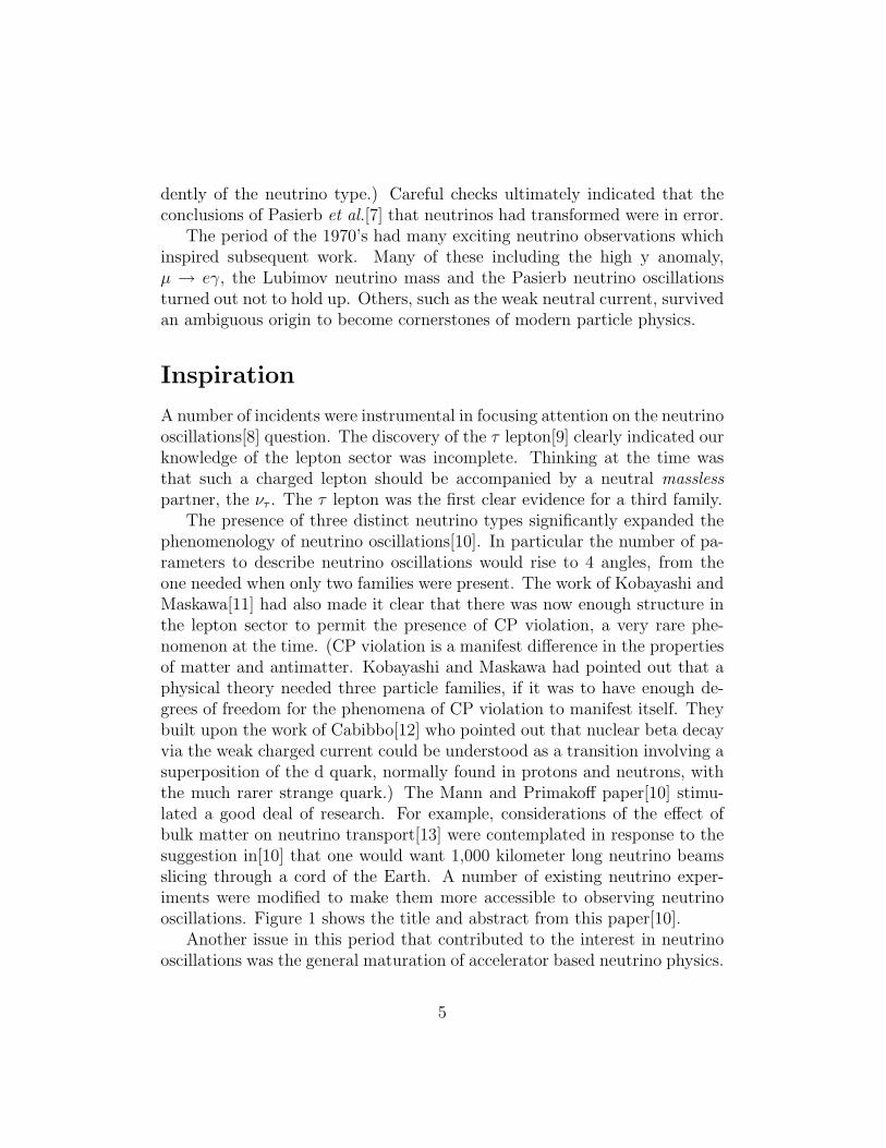
dently of the neutrino type.) Careful checks ultimately indicated that theconclusions of Pasierb et al.[7] that neutrinos had transformed were in error.

The period of the 1970’s had many exciting neutrino observations whichinspired subsequent work. Many of these including the high y anomaly,µ → eγ, the Lubimov neutrino mass and the Pasierb neutrino oscillationsturned out not to hold up. Others, such as the weak neutral current, survivedan ambiguous origin to become cornerstones of modern particle physics.

Inspiration

A number of incidents were instrumental in focusing attention on the neutrinooscillations[8] question. The discovery of the τ lepton[9] clearly indicated ourknowledge of the lepton sector was incomplete. Thinking at the time wasthat such a charged lepton should be accompanied by a neutral masslesspartner, the ντ . The τ lepton was the first clear evidence for a third family.

The presence of three distinct neutrino types significantly expanded thephenomenology of neutrino oscillations[10]. In particular the number of pa-rameters to describe neutrino oscillations would rise to 4 angles, from theone needed when only two families were present. The work of Kobayashi andMaskawa[11] had also made it clear that there was now enough structure inthe lepton sector to permit the presence of CP violation, a very rare phe-nomenon at the time. (CP violation is a manifest difference in the propertiesof matter and antimatter. Kobayashi and Maskawa had pointed out that aphysical theory needed three particle families, if it was to have enough de-grees of freedom for the phenomena of CP violation to manifest itself. Theybuilt upon the work of Cabibbo[12] who pointed out that nuclear beta decayvia the weak charged current could be understood as a transition involving asuperposition of the d quark, normally found in protons and neutrons, withthe much rarer strange quark.) The Mann and Primakoff paper[10] stimu-lated a good deal of research. For example, considerations of the effect ofbulk matter on neutrino transport[13] were contemplated in response to thesuggestion in[10] that one would want 1,000 kilometer long neutrino beamsslicing through a cord of the Earth. A number of existing neutrino exper-iments were modified to make them more accessible to observing neutrinooscillations. Figure 1 shows the title and abstract from this paper[10].

Another issue in this period that contributed to the interest in neutrinooscillations was the general maturation of accelerator based neutrino physics.

5

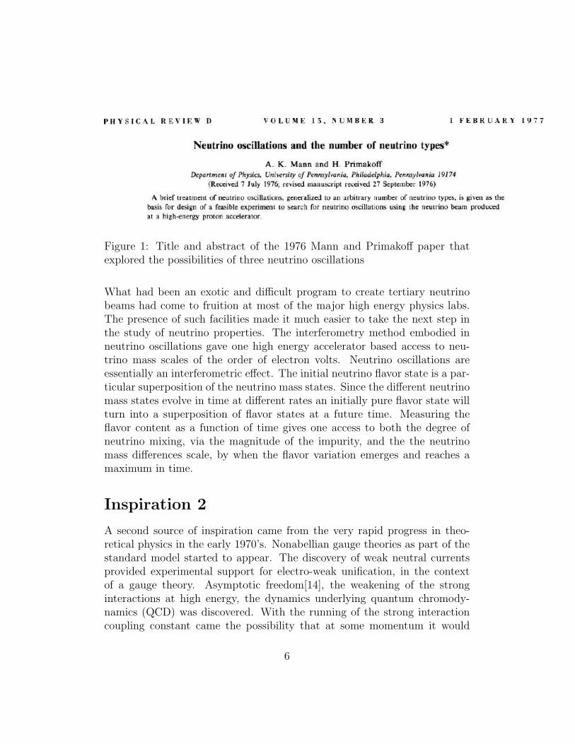
Figure 1: Title and abstract of the 1976 Mann and Primakoff paper thatexplored the possibilities of three neutrino oscillations

What had been an exotic and difficult program to create tertiary neutrinobeams had come to fruition at most of the major high energy physics labs.The presence of such facilities made it much easier to take the next step inthe study of neutrino properties. The interferometry method embodied inneutrino oscillations gave one high energy accelerator based access to neu-trino mass scales of the order of electron volts. Neutrino oscillations areessentially an interferometric effect. The initial neutrino flavor state is a par-ticular superposition of the neutrino mass states. Since the different neutrinomass states evolve in time at different rates an initially pure flavor state willturn into a superposition of flavor states at a future time. Measuring theflavor content as a function of time gives one access to both the degree ofneutrino mixing, via the magnitude of the impurity, and the the neutrinomass differences scale, by when the flavor variation emerges and reaches amaximum in time.

Inspiration 2

A second source of inspiration came from the very rapid progress in theo-retical physics in the early 1970’s. Nonabellian gauge theories as part of thestandard model started to appear. The discovery of weak neutral currentsprovided experimental support for electro-weak unification, in the contextof a gauge theory. Asymptotic freedom[14], the weakening of the stronginteractions at high energy, the dynamics underlying quantum chromody-namics (QCD) was discovered. With the running of the strong interactioncoupling constant came the possibility that at some momentum it would

6

meet the electro-weak value and Grand Unified theories[15] (GUTS) werecreated. These theories combined three forces of nature into one large groupand demonstrated how the underlying distinctions would emerge at normalenergies. At some high energy. called the unification scale all the interactionswould be identical, with the same interaction strength. At lower energies thecoupling constants and selection rules would diverge to form, what appearto be three distinct forces of nature.

Such unification was not without cost. Rather quickly it was realizedthat some of the additional interactions present in Grand Unified theorieswould lead to new, rare phenomena[16], such as the decay of the proton toleptons and mesons. The final state would conserve electric charge, angularmomentum or spin and energy but it would not conserve the values of baryonnumber or lepton number. The theory was not in conflict with observationsince the lifetime predicted was still several orders of magnitude longer thanexperimental limits on proton decay at the time.

The possibility of experimental confirmation of Grand Unified theoriesvia the observation of proton decay became a goal of late 1970’s to early1990’s particle physics and is still important today. No convincing evidencehas been reported for proton instability. Even now, the best we have areupper limits on its lifetime. The story of how technical problems were solvedto reduce costs such that massive detectors capable of making interestingmeasurements of the proton lifetime is a long one that we can not discusshere. A recent talk[17] outlines how the major design decisions were madein the period 1978-1979 and the first detectors constructed by 1982.

Much of the work described in the current paper took place in the con-text of a collaboration centered at the University of California at Irvine,the University of Michigan and Brookhaven National Laboratory, known asIMB. The collaboration was formed in early 1979 to construct a massive deepunderground detector to discover proton decay. The Irvine group includedmany of the co-discoverers of atmospheric neutrinos.

Figure 2 is a sketch of the detector used for this research. Reference [18]describes the search for proton decay and includes photographs and otherillustrations of the methods employed.

Most early Grand Unified theories predicted that the proton would decayto a final state consisting of a positron and a neutral pion. The neutral pionwould immediately decay to two photons giving a fairly clear signal. Somevariations of the theories, including those incorporating supersymmetry pre-dicted suppression of this decay mode but favored a decay mode containing

7

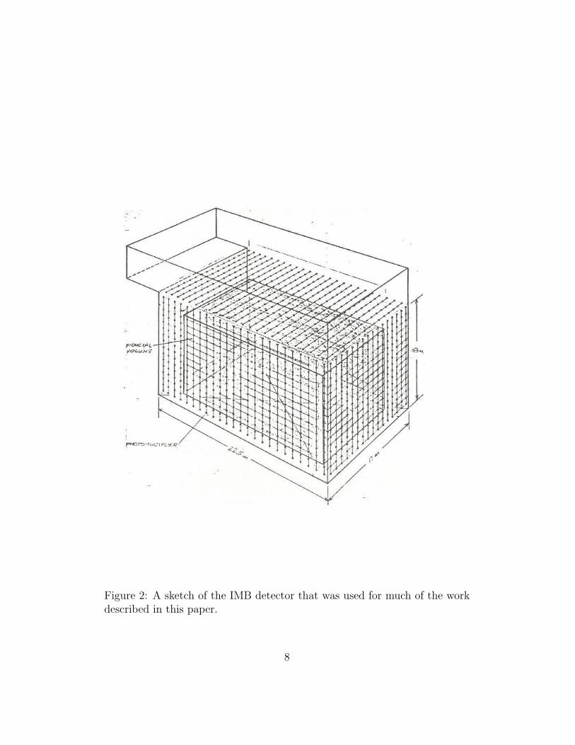
Figure 2: A sketch of the IMB detector that was used for much of the workdescribed in this paper.

8

a charged muon and a neutral K meson. The neutral K meson would alsodecay yielding a somewhat different signature. Some ability to distinguishthe proton decay modes was an essential part of the experiments.

An experiment searching for a rare processes such as proton decay mustbe very sensitive. A sensitive detector is subject to a very large numberof detections of non-signal. Such non-signal is termed “background”. Aproton decay detector needs to be very large to be sensitive to the signalbut it must be well shielded to reduce the background to a level where itdoes not obscure the signal. All such low background experiments have beenlocated underground since cosmic rays produce a substantial contribution tothe background at the surface. Even underground the cosmic ray rate is atbest reduced but never eliminated. This is because the high energy muoncomponent of the surface cosmic rays interact primarily electromagneticallyand so they loose energy fairly slowly in traversing matter. As a rule, thedeeper the detector the fewer cosmic ray muons one must register and reject.One important trade-off is that excavation costs are higher the deeper onegoes. So on a fixed budget one would have to construct a smaller detectorat larger depths. In most cases the location of the underground laboratoryhas been determined by previously existing infrastructure such as a mine ormountain tunnel.

One form of non-signal, background, which is not attenuated by depthare interactions from the neutrinos produced by cosmic ray interactions inthe atmosphere. A very efficient method for producing neutrinos in theatmosphere is by strong interaction production of pions. The pions decayreadily to a muon and a muon neutrino. Many of the muons also decay beforethey reach the ground to yield an electron and two additional neutrinos (oneeach of electron and muon type). Neutrinos are very penetrating since theyonly interact via the weak interaction, so they are essentially unattenuatedby any amount of terrestrial shielding.

The flux of these neutrinos can be calculated and an event rate estimated.The experimental challenge was to identify neutrino interactions so that theycould not be confused with the proton decay signature. In principle it wouldbe easy to distinguish the two. Protons decayed essentially at rest in thedetector, with negligible momentum whereas entering neutrinos bring mo-mentum creating events with approximately equal energy and momentum.So one can distinguish the two classes of events by reconstructing the eventsan measuring their momentum.

9

Formulation I – Accelerator Experiments

The search for neutrino oscillations was begun most expeditiously by adapt-ing existing facilities to the project. Once existing data had been checked,and no evidence for oscillations found, the next step was to try to extend therange of the searches. One project, experiment 704 at Brookhaven, utilizeda neutrino detector that had been used to establish the properties of theweak neutral current[19]. To extend its sensitivity to neutrino oscillationsthe energy of the beam was lowered. Lowering the neutrino beam energyhad several advantages. It extended the sensitivity to lower neutrino massdifferences (∆m2). At the lower energies the muon neutrinos in the beamwould not interact because they had insufficient center of mass energy toproduce a muon via the charged current interaction. Interactions could onlyoccur if the muon neutrinos transformed into electron neutrinos. Loweringthe production energy also had the advantage that no electron neutrinos wereproduced in the target since the beam was below kaon production threshold.Kaons are the major source of the electron neutrino content of acceleratorbased neutrino beams.

The experiment failed to find evidence for neutrino oscillations but gavethe experimenters, many of whom went on to work on IMB, substantialexperience with the neutrino oscillations problem. Figure 4 shows many ofthe participants in this early oscillations experiment.

Formulation II – Neutrinos in Nature

While the flux of atmospheric neutrinos was an annoyance to the search forproton decay, it was realized that such a signal also provided an opportunityto extended the study of neutrino oscillations to kinematic regions of massdifferences, ∆m2 well below what would be feasible at accelerators or reac-tors. But to be effective the detector would have to be able to distinguishbetween different kinds of neutrino interactions. Fortunately the requirementto identify the proton decay final state to distinguish different models hadsimilar requirements. The IMB detector[20] was designed with a high reso-lution time scale to facilitate reconstruction by time of flight and a coarsetime resolution which extended out to 10 microseconds following an eventto search for a delayed signal coming from a final state muon, µ → eνν̄(Figure 5). This coarse time scale, or second time scale was known as the

10

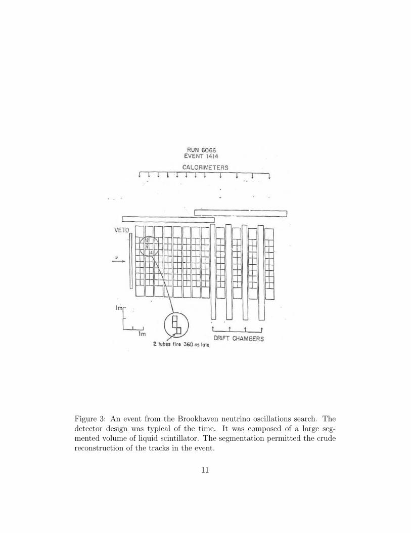
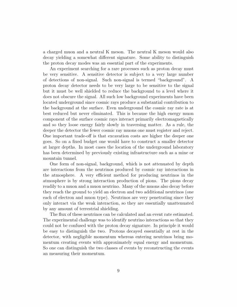
Figure 3: An event from the Brookhaven neutrino oscillations search. Thedetector design was typical of the time. It was composed of a large seg-mented volume of liquid scintillator. The segmentation permitted the crudereconstruction of the tracks in the event.

11

Figure 4: Members of a dedicated neutrino oscillations experiment atBrookhaven National Laboratory in 1977. LoSecco is on the left and LarrySulak is kneeling on the right. Bill Wang is kneeling to the right of LoSecco.Andy Soukas is in the middle of the group of accelerator operators standingin the back.

12

“T2” scale and was to later give the name “T2 problem” to our discovery.While massive shielded underground detectors were motivated, and fundedinitially to experimentally observe predictions of Grand Unified theories, itis noteworthy that even the earliest proposals[20] clearly indicated that suchdetectors would also be able to explore “neutrino oscillations, matter effectsand supernovae”. The groups active in the search for proton decay, for themost part, had substantial neutrino experience since the problems were sim-ilar in many ways. Neutrino observation also required massive well shieldeddetectors.

While the IMB proposal[20] had mentioned neutrino oscillations the de-tails were not filled in until spring of 1980. As part of the graduate schoolrequirements at Harvard University, students were expected to prepare aproject on a topic related to their thesis research and to present it as an oralexam. Bruce Cortez, a student of Larry Sulak, chose atmospheric neutrinooscillations as his qualifying orals topic[21]. His work was fairly complete.It included details of the neutrino flight distance as a function of direction.Upward going neutrinos travel about 13,000 km but those going down onlytravel about 15 km. While, in principle one got all of the distances in be-tween the transition from up to down distance scales occurs very rapidlyover a fairly small part of the total solid angle near the horizon so, in essenceone was dealing with an approximately 2 distance neutrino experiment. Thecorrelation of neutrino direction, with the direction reconstructed from thefinal states was studied. For most neutrino events the reconstructed direc-tion of the outgoing muon or electron provides a reasonable estimate of theneutrino direction (and hence path length) but this concordance tends tobe less reliable at lower energies. Fortunately the problem does not preventtelling up from down. The work showed that for about two orders of mag-nitude ∆m2, from below 10−4 eV2 to about 10−2 eV2 one would have a veryclear difference in the electron to muon ratio measured for upward eventscompared to the observed value for downward events. The downward eventsprovided a short range sample to which the long range upward going eventscould be compared. Figures prepared for this work also showed a substantialdistortion in the neutrino spectra if ∆m2 were in a range just below or justabove the one where the effect would be maximal. The Cortez oral workwas documented in a number of conference talks[22, 23]. Figures 6 and 7are the title pages from some of these talks. Figure 8 summarizes most ofthe information needed to study atmospheric neutrino oscillations includingthe neutrino flux and cross sections, the variable distances and resolution

13

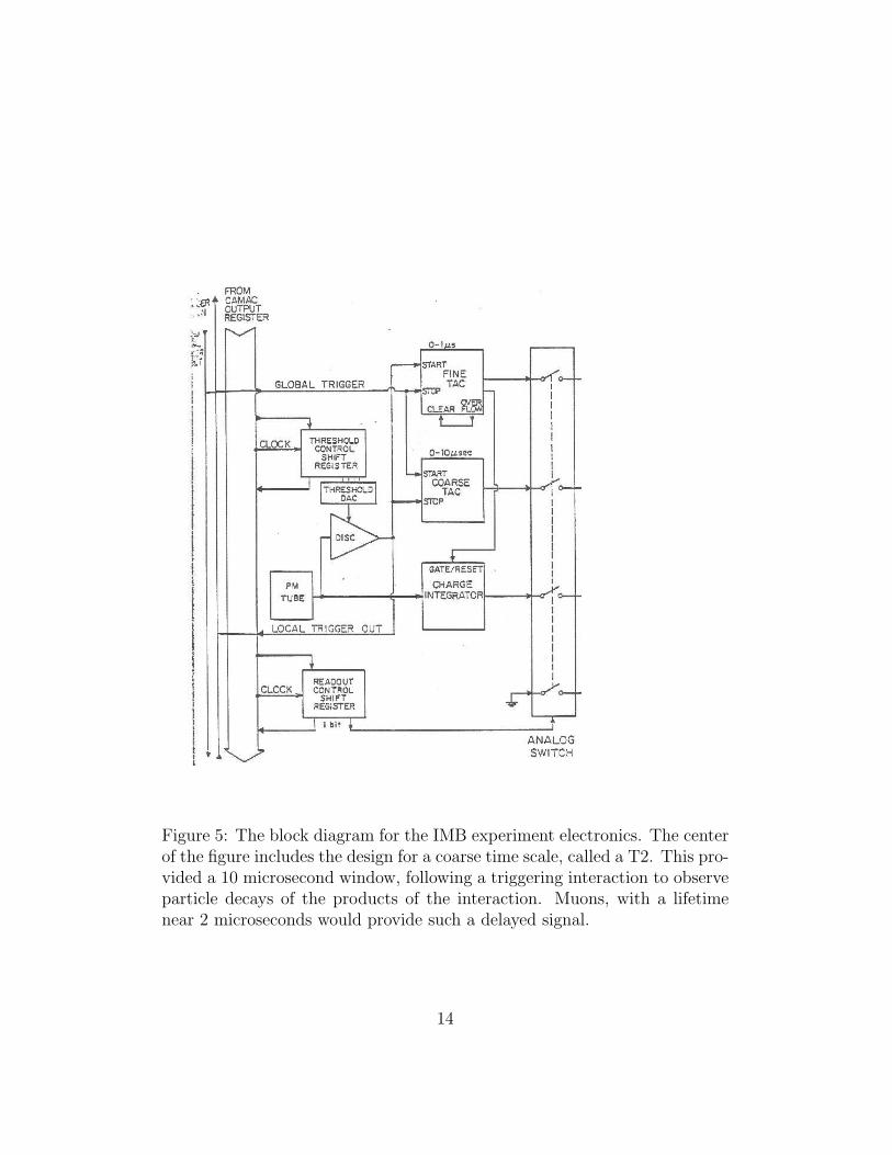
Figure 5: The block diagram for the IMB experiment electronics. The centerof the figure includes the design for a coarse time scale, called a T2. This pro-vided a 10 microsecond window, following a triggering interaction to observeparticle decays of the products of the interaction. Muons, with a lifetimenear 2 microseconds would provide such a delayed signal.

14

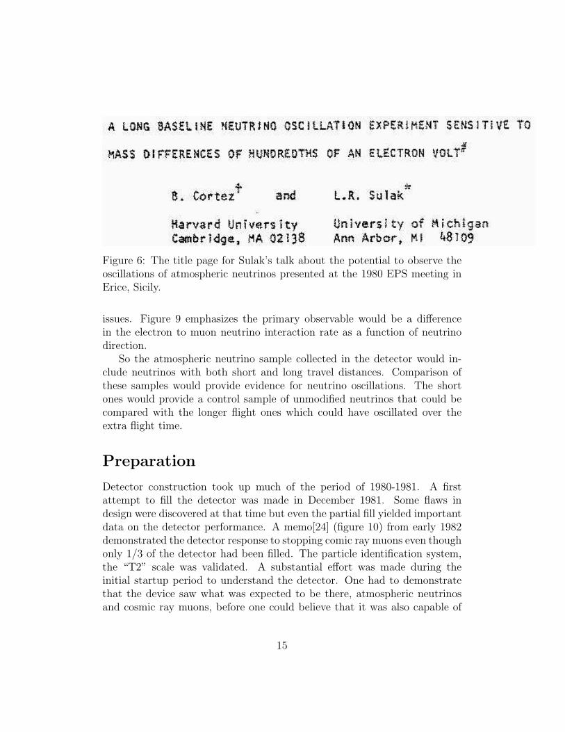
Figure 6: The title page for Sulak’s talk about the potential to observe theoscillations of atmospheric neutrinos presented at the 1980 EPS meeting inErice, Sicily.

issues. Figure 9 emphasizes the primary observable would be a differencein the electron to muon neutrino interaction rate as a function of neutrinodirection.

So the atmospheric neutrino sample collected in the detector would in-clude neutrinos with both short and long travel distances. Comparison ofthese samples would provide evidence for neutrino oscillations. The shortones would provide a control sample of unmodified neutrinos that could becompared with the longer flight ones which could have oscillated over theextra flight time.

Preparation

Detector construction took up much of the period of 1980-1981. A firstattempt to fill the detector was made in December 1981. Some flaws indesign were discovered at that time but even the partial fill yielded importantdata on the detector performance. A memo[24] (figure 10) from early 1982demonstrated the detector response to stopping comic ray muons even thoughonly 1/3 of the detector had been filled. The particle identification system,the “T2” scale was validated. A substantial effort was made during theinitial startup period to understand the detector. One had to demonstratethat the device saw what was expected to be there, atmospheric neutrinosand cosmic ray muons, before one could believe that it was also capable of

15

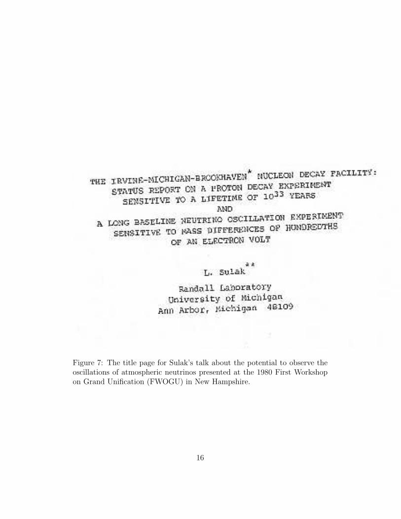
Figure 7: The title page for Sulak’s talk about the potential to observe theoscillations of atmospheric neutrinos presented at the 1980 First Workshopon Grand Unification (FWOGU) in New Hampshire.

16

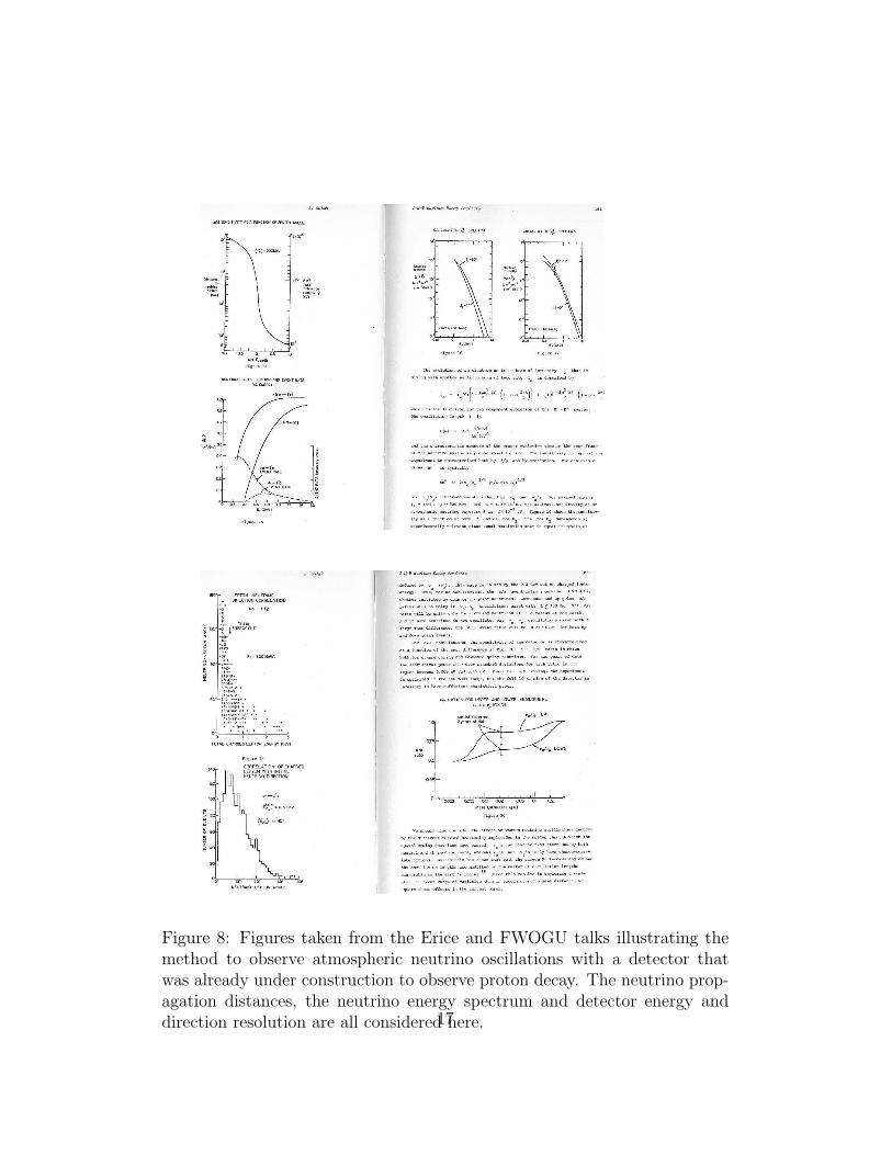
Figure 8: Figures taken from the Erice and FWOGU talks illustrating themethod to observe atmospheric neutrino oscillations with a detector thatwas already under construction to observe proton decay. The neutrino prop-agation distances, the neutrino energy spectrum and detector energy anddirection resolution are all considered here.17

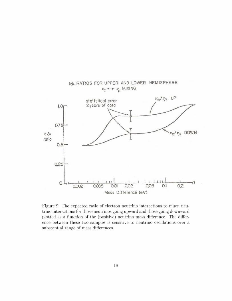
Figure 9: The expected ratio of electron neutrino interactions to muon neu-trino interactions for those neutrinos going upward and those going downwardplotted as a function of the (positive) neutrino mass difference. The differ-ence between these two samples is sensitive to neutrino oscillations over asubstantial range of mass differences.

18

Figure 10: Heading from a 1982 internal report on calibrating the detectorresponse to muon decays. This work was done well before the detector wascompleted

19

observing proton decay.Since the atmospheric neutrinos were expected to be the only serious

background to proton decay several efforts were made to control systematicerrors associated with them. The atmospheric neutrino response in the detec-tor was modeled using real neutrino interactions. We had access to the largesample of accelerator neutrino interactions acquired at CERN in the heavyliquid bubble chamber “Gargamelle”. These interactions were primarily onbromine, a slightly heavier nucleus than the oxygen found in our water. Butwe needed a sample of neutrino interactions on nuclei since these would in-clude absorption, rescattering and Fermi motion effects caused by the othernucleons in the nucleus. Subsequent to the work with the “Gargamelle”events we also studied events on neon from Brookhaven and on deuteriumfrom Argonne. Several neutrino interaction models were also prepared tofacilitate comparison and gauge systematic error.

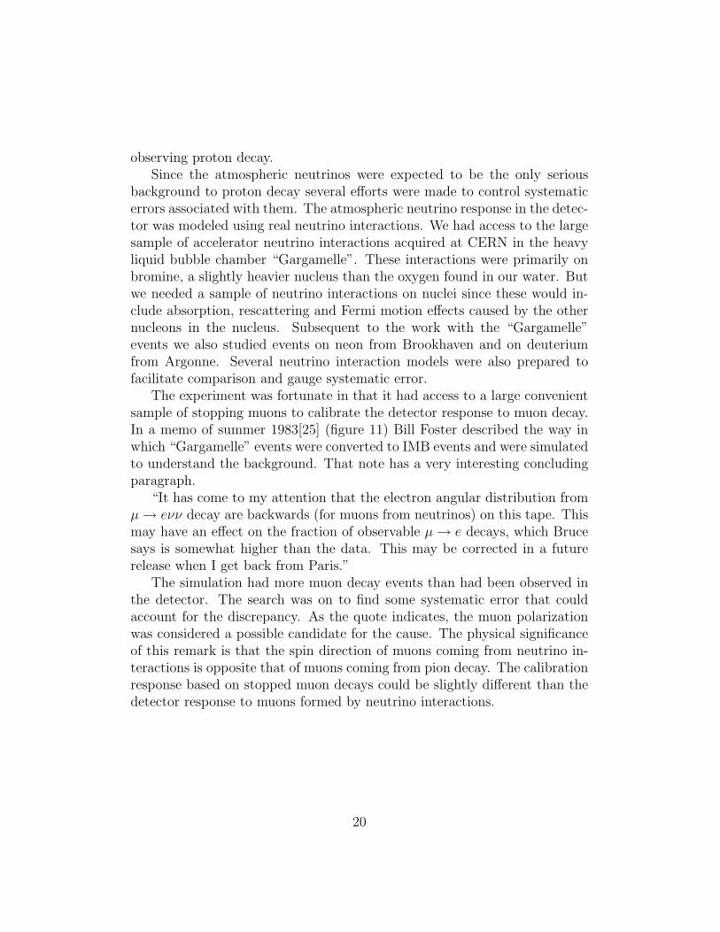
The experiment was fortunate in that it had access to a large convenientsample of stopping muons to calibrate the detector response to muon decay.In a memo of summer 1983[25] (figure 11) Bill Foster described the way inwhich “Gargamelle” events were converted to IMB events and were simulatedto understand the background. That note has a very interesting concludingparagraph.

“It has come to my attention that the electron angular distribution fromµ → eνν decay are backwards (for muons from neutrinos) on this tape. Thismay have an effect on the fraction of observable µ → e decays, which Brucesays is somewhat higher than the data. This may be corrected in a futurerelease when I get back from Paris.”

The simulation had more muon decay events than had been observed inthe detector. The search was on to find some systematic error that couldaccount for the discrepancy. As the quote indicates, the muon polarizationwas considered a possible candidate for the cause. The physical significanceof this remark is that the spin direction of muons coming from neutrino in-teractions is opposite that of muons coming from pion decay. The calibrationresponse based on stopped muon decays could be slightly different than thedetector response to muons formed by neutrino interactions.

20

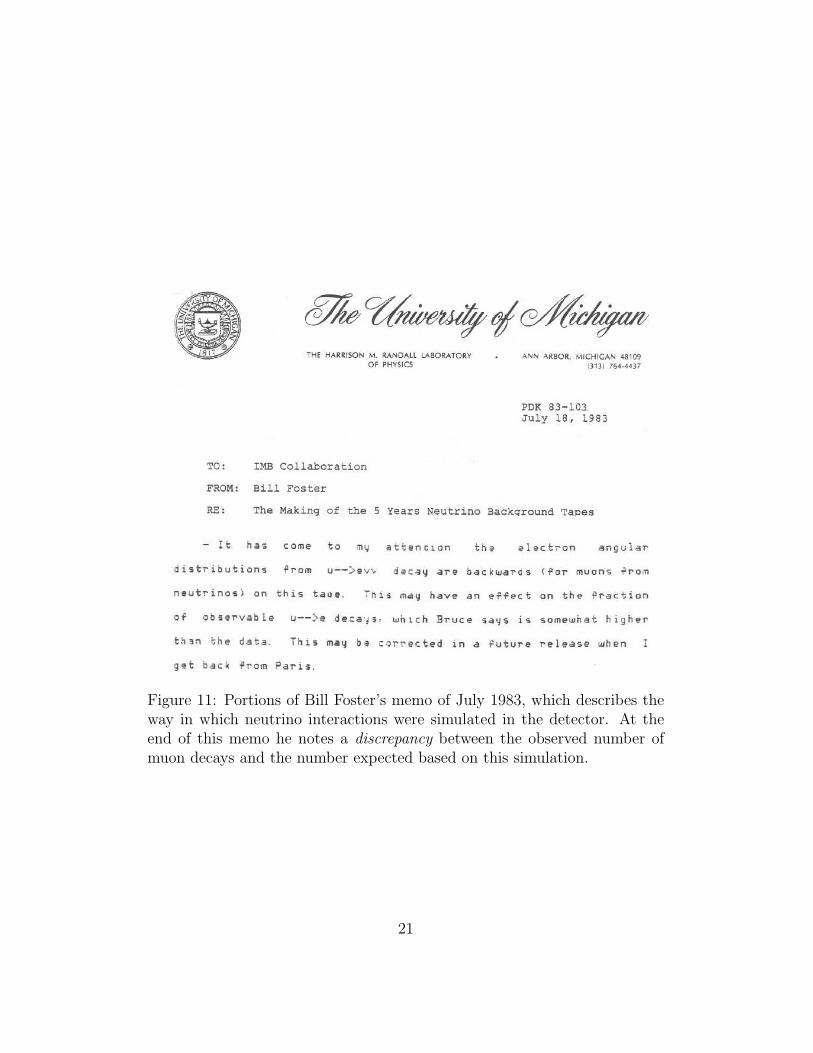
Figure 11: Portions of Bill Foster’s memo of July 1983, which describes theway in which neutrino interactions were simulated in the detector. At theend of this memo he notes a discrepancy between the observed number ofmuon decays and the number expected based on this simulation.

21

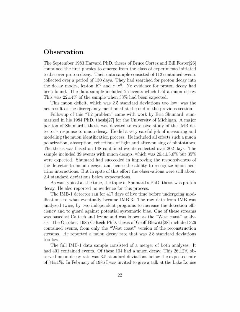
Observation

The September 1983 Harvard PhD. theses of Bruce Cortez and Bill Foster[26]contained the first physics to emerge from the class of experiments initiatedto discover proton decay. Their data sample consisted of 112 contained eventscollected over a period of 130 days. They had searched for proton decay intothe decay modes, lepton K0 and e+π0. No evidence for proton decay hadbeen found. The data sample included 25 events which had a muon decay.This was 22±4% of the sample when 33% had been expected.

This muon deficit, which was 2.5 standard deviations too low, was thenet result of the discrepancy mentioned at the end of the previous section.

Followup of this “T2 problem” came with work by Eric Shumard, sum-marized in his 1984 PhD. thesis[27] for the University of Michigan. A majorportion of Shumard’s thesis was devoted to extensive study of the IMB de-tector’s response to muon decay. He did a very careful job of measuring andmodeling the muon identification process. He included all effects such a muonpolarization, absorption, reflections of light and after-pulsing of phototubes.The thesis was based on 148 contained events collected over 202 days. Thesample included 39 events with muon decays, which was 26.4±3.6% but 35%were expected. Shumard had succeeded in improving the responsiveness ofthe detector to muon decays, and hence the ability to recognize muon neu-trino interactions. But in spite of this effort the observations were still about2.4 standard deviations below expectations.

As was typical at the time, the topic of Shumard’s PhD. thesis was protondecay. He also reported no evidence for this process.

The IMB-1 detector ran for 417 days of live time before undergoing mod-ifications to what eventually became IMB-3. The raw data from IMB wasanalyzed twice, by two independent programs to increase the detection effi-ciency and to guard against potential systematic bias. One of these streamswas based at Caltech and Irvine and was known as the “West coast” analy-sis. The October, 1985 Caltech PhD. thesis of Geoff Blewitt[28] included 326contained events, from only the “West coast” version of the reconstructionstreams. He reported a muon decay rate that was 2.8 standard deviationstoo low.

The full IMB-1 data sample consisted of a merger of both analyses. Ithad 401 contained events. Of these 104 had a muon decay. This 26±2% ob-served muon decay rate was 3.5 standard deviations below the expected rateof 34±1%. In February of 1986 I was invited to give a talk at the Lake Louise

22

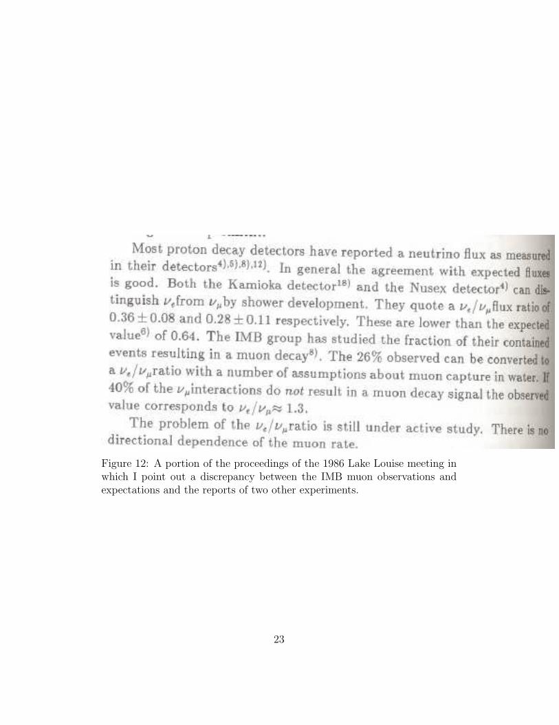
Figure 12: A portion of the proceedings of the 1986 Lake Louise meeting inwhich I point out a discrepancy between the IMB muon observations andexpectations and the reports of two other experiments.

23

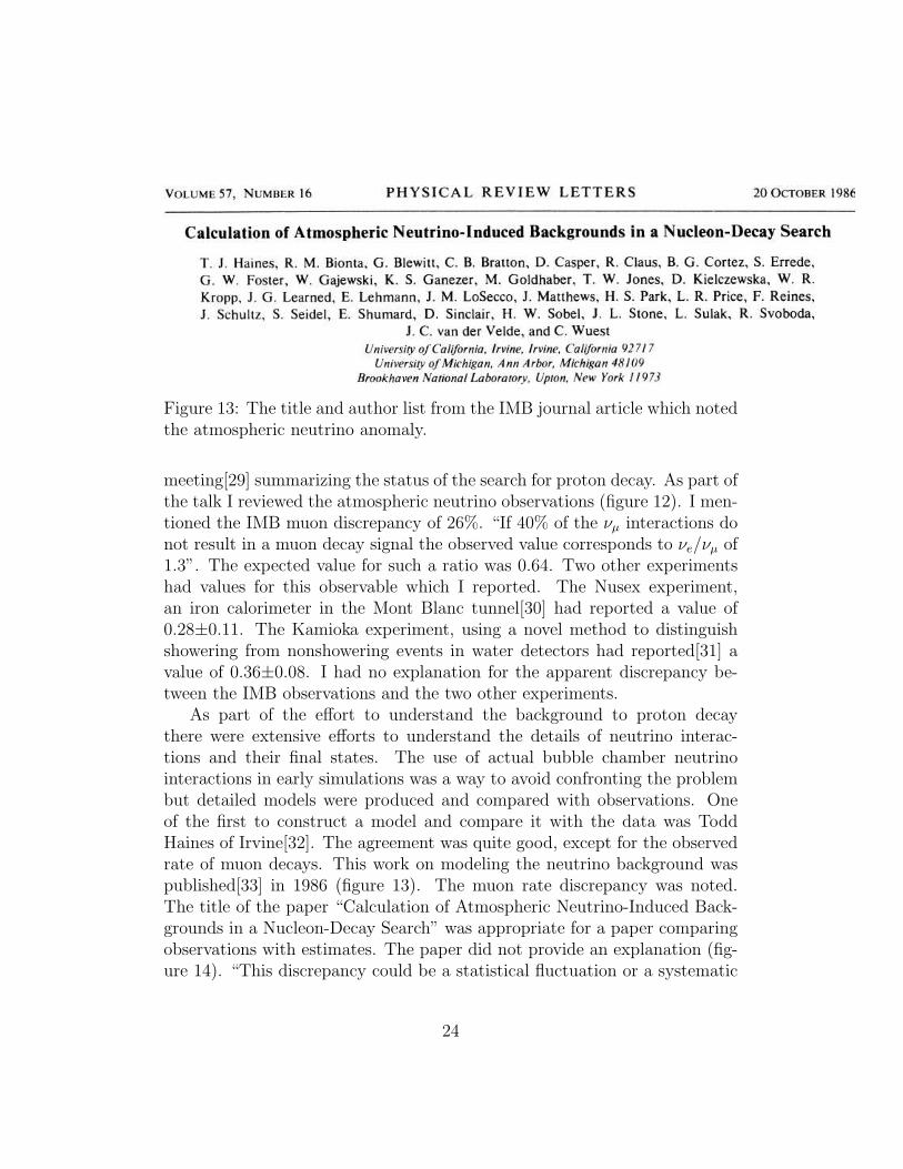
Figure 13: The title and author list from the IMB journal article which notedthe atmospheric neutrino anomaly.

meeting[29] summarizing the status of the search for proton decay. As part ofthe talk I reviewed the atmospheric neutrino observations (figure 12). I men-tioned the IMB muon discrepancy of 26%. “If 40% of the νµ interactions donot result in a muon decay signal the observed value corresponds to νe/νµ of1.3”. The expected value for such a ratio was 0.64. Two other experimentshad values for this observable which I reported. The Nusex experiment,an iron calorimeter in the Mont Blanc tunnel[30] had reported a value of0.28±0.11. The Kamioka experiment, using a novel method to distinguishshowering from nonshowering events in water detectors had reported[31] avalue of 0.36±0.08. I had no explanation for the apparent discrepancy be-tween the IMB observations and the two other experiments.

As part of the effort to understand the background to proton decaythere were extensive efforts to understand the details of neutrino interac-tions and their final states. The use of actual bubble chamber neutrinointeractions in early simulations was a way to avoid confronting the problembut detailed models were produced and compared with observations. Oneof the first to construct a model and compare it with the data was ToddHaines of Irvine[32]. The agreement was quite good, except for the observedrate of muon decays. This work on modeling the neutrino background waspublished[33] in 1986 (figure 13). The muon rate discrepancy was noted.The title of the paper “Calculation of Atmospheric Neutrino-Induced Back-grounds in a Nucleon-Decay Search” was appropriate for a paper comparingobservations with estimates. The paper did not provide an explanation (fig-ure 14). “This discrepancy could be a statistical fluctuation or a systematic

24

Figure 14: Excerpt from the 1986 IMB neutrino paper describing the atmo-spheric neutrino anomaly and some potential explanations. The variety ofexplanations represented the varied opinions of the multiple authors.

error due to (i) an incorrect assumption as to the ratio of muon ν’s to elec-tron ν’s in the atmospheric fluxes, (ii) an incorrect estimate of the efficiencyfor our observing a muon decay, or (iii) some other as-yet-unaccounted-forphysics.” The diversity of interpretations reflected the diverse opinions of theauthors. In reality, the first two possible hypotheses could at best reduce thestatistical significance of the result. Any uncertainty in the flux or the muondecay rate could not correct for the apparent 40% reduction in the muonneutrino interaction rate the observations suggested. The large scale of theanomaly was reflected in my Lake Louise quote above. After correcting forinefficiencies the data was almost a factor of 2 off from expectations. It isnoteworthy that most collaborations, including IMB can be very conserva-tive. As can be clearly seen in many documents leading up to this period,such as the PhD. theses quoted, most people hoped that the effect wouldjust go away. In fact the muon decay deficiency was not mentioned in earlydrafts of the 1986 article. It was added, at my insistence, since the topicof the paper, comparing neutrino observations with expectations, seemedappropriate.

25

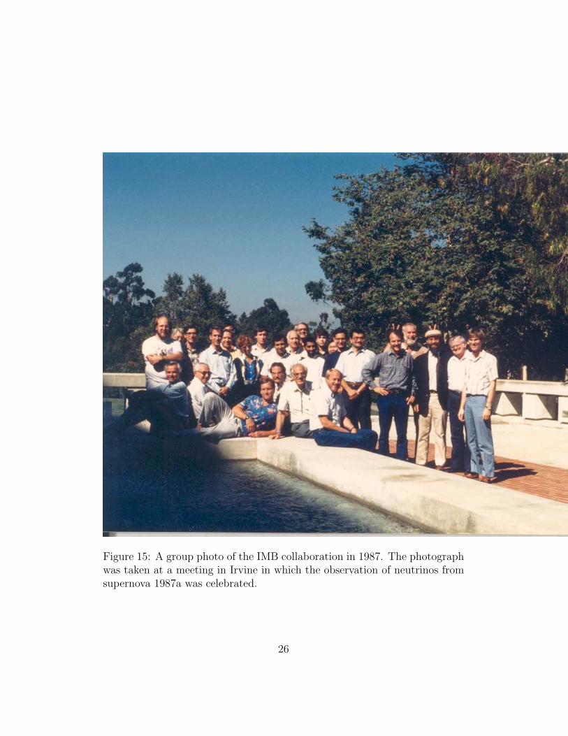
Figure 15: A group photo of the IMB collaboration in 1987. The photographwas taken at a meeting in Irvine in which the observation of neutrinos fromsupernova 1987a was celebrated.

26

While people have voiced criticism of the wording used in this[33] paper,because of the multiple hypotheses provided. The multiple hypotheses wasa compromise among the authors that permitted a significant but not fullyunderstood effect to be reported to a larger audience. The error reported onthe observed muon decay rate in the published letter[33] was±3% rather thanthe ±2% mentioned earlier. The smaller value, calculated using Binomialstatistics is right. Binomial statistics is the correct way to estimate the errorsince this ensures that the error on the fraction of events with a muon decayis exactly the same as the error on the fraction of events without a muondecay. The error can be easily calculated from the numbers in the paper.

Interpretation

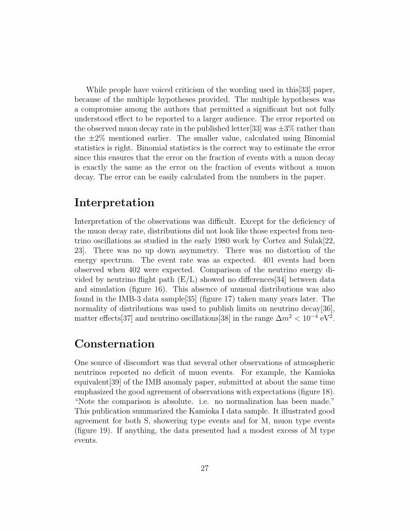
Interpretation of the observations was difficult. Except for the deficiency ofthe muon decay rate, distributions did not look like those expected from neu-trino oscillations as studied in the early 1980 work by Cortez and Sulak[22,23]. There was no up down asymmetry. There was no distortion of theenergy spectrum. The event rate was as expected. 401 events had beenobserved when 402 were expected. Comparison of the neutrino energy di-vided by neutrino flight path (E/L) showed no differences[34] between dataand simulation (figure 16). This absence of unusual distributions was alsofound in the IMB-3 data sample[35] (figure 17) taken many years later. Thenormality of distributions was used to publish limits on neutrino decay[36],matter effects[37] and neutrino oscillations[38] in the range ∆m2 < 10−4 eV2.

Consternation

One source of discomfort was that several other observations of atmosphericneutrinos reported no deficit of muon events. For example, the Kamiokaequivalent[39] of the IMB anomaly paper, submitted at about the same timeemphasized the good agreement of observations with expectations (figure 18).“Note the comparison is absolute. i.e. no normalization has been made.”This publication summarized the Kamioka I data sample. It illustrated goodagreement for both S, showering type events and for M, muon type events(figure 19). If anything, the data presented had a modest excess of M typeevents.

27

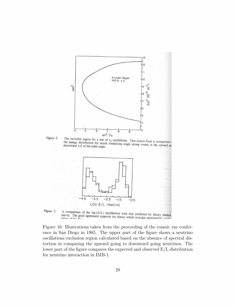
Figure 16: Illustrations taken from the proceeding of the cosmic ray confer-ence in San Diego in 1985. The upper part of the figure shows a neutrinooscillations exclusion region calculated based on the absence of spectral dis-tortion in comparing the upward going to downward going neutrinos. Thelower part of the figure compares the expected and observed E/L distributionfor neutrino interaction in IMB-1.

28

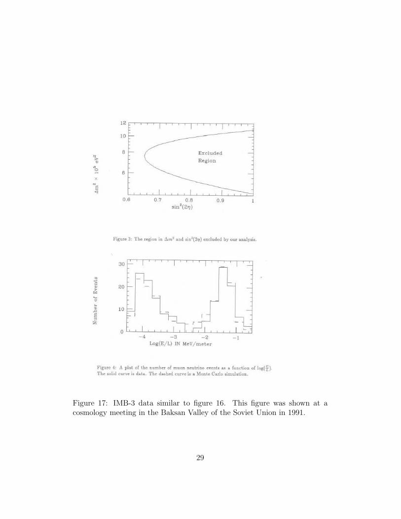
Figure 17: IMB-3 data similar to figure 16. This figure was shown at acosmology meeting in the Baksan Valley of the Soviet Union in 1991.

29

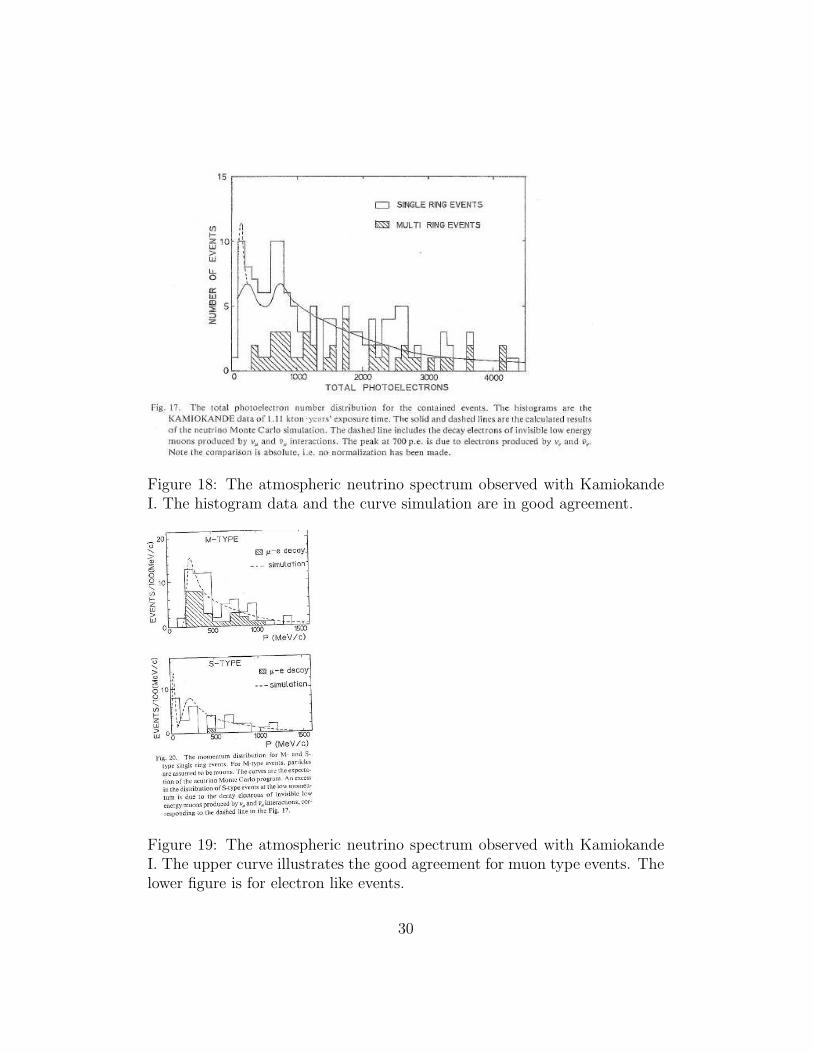
Figure 18: The atmospheric neutrino spectrum observed with KamiokandeI. The histogram data and the curve simulation are in good agreement.

Figure 19: The atmospheric neutrino spectrum observed with KamiokandeI. The upper curve illustrates the good agreement for muon type events. Thelower figure is for electron like events.

30

The Kamioka detector had much more light collection capability than theIMB detector. This permitted them to utilize the shape of the Cherenkovimage to determine if the interaction had produced a muon, M type events,or an electron, S type events. The S stands for showering since the electronwould multiple scatter, bremsstrahlung and pair produce. A processes knownas an electromagnetic shower. Muon induced events had a much crisper,cleaner image. Kamioka had used this difference in images to distinguishelectron from muon type events.

While Nakahata et al.[39] had no numbers for data, the data was thesame as the Kajita PhD. thesis[43] from earlier in 1986. Kajita’s PhD.thesis[43] reported the observations from the first phase of Kamioka, knownas Kamiokande I. In an exposure of 1.11 kt-yr they reported 141 containedevent in 474 days of live time. The ability to distinguish showering fromnon-showering tracks permitted them to report the event rates in the twocategories.

They reported 97 single prong events (89 with energies above 100 MeV)when they expected to observe 94 (85 with energies above 100 MeV). So thereported event rate was as expected. They reported 64 M type, or muon type,events when 54 were expected. They reported 33 S type events, electrons (25above 100 MeV) when 40 were expected (31 above 100 MeV). The reason formentioning the S type event rate above 100 MeV is that muon decay fromsub threshold muons could look like showering low energy electron events.Cosmic ray sub threshold muons could slip into the device undetected andlook like low energy electron neutrino interactions.

The Kamiokande I detector was capable of recording delayed muon de-cays associated with an event. 29 events had muon decays when 39.3 wereexpected.

These numbers are all in the thesis[43]. The thesis conclusions are thatthe muon and electron fractions are as expected.

But the numbers quoted above clearly indicate a 2.4 standard deviationdeficiency of muon decay signals and a 1.6 standard deviation excess of Mtype events, when compared to expectations. None of these significances arecalculated in the thesis.

In June of 1986 I visited Tokyo following the neutrino meeting at Sendai.I met with Koshiba and Kajita. I was well received. Koshiba took me anda small contingent of his group to a nearby noodle restaurant for a lesson inthe art of slurping. The IMB anomaly paper had recently been submitted forpublication. I discussed our observed muon decay deficiency. I pointed out

31

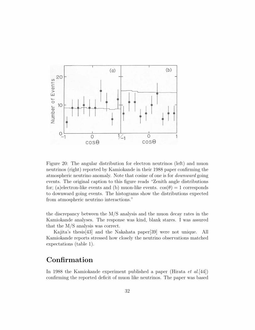
Figure 20: The angular distribution for electron neutrinos (left) and muonneutrinos (right) reported by Kamiokande in their 1988 paper confirming theatmospheric neutrino anomaly. Note that cosine of one is for downward goingevents. The original caption to this figure reads “Zenith angle distributionsfor; (a)electron-like events and (b) muon-like events. cos(θ) = 1 correspondsto downward going events. The histograms show the distributions expectedfrom atmospheric neutrino interactions.”

the discrepancy between the M/S analysis and the muon decay rates in theKamiokande analyses. The response was kind, blank stares. I was assuredthat the M/S analysis was correct.

Kajita’s thesis[43] and the Nakahata paper[39] were not unique. AllKamiokande reports stressed how closely the neutrino observations matchedexpectations (table 1).

Confirmation

In 1988 the Kamiokande experiment published a paper (Hirata et al.[44])confirming the reported deficit of muon like neutrinos. The paper was based

32

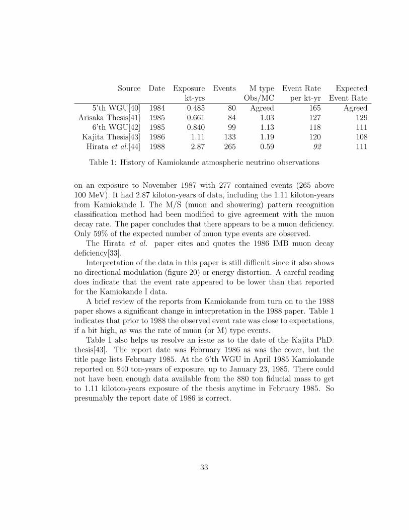
Source Date Exposure Events M type Event Rate Expectedkt-yrs Obs/MC per kt-yr Event Rate

5’th WGU[40] 1984 0.485 80 Agreed 165 AgreedArisaka Thesis[41] 1985 0.661 84 1.03 127 129

6’th WGU[42] 1985 0.840 99 1.13 118 111Kajita Thesis[43] 1986 1.11 133 1.19 120 108Hirata et al.[44] 1988 2.87 265 0.59 92 111

Table 1: History of Kamiokande atmospheric neutrino observations

on an exposure to November 1987 with 277 contained events (265 above100 MeV). It had 2.87 kiloton-years of data, including the 1.11 kiloton-yearsfrom Kamiokande I. The M/S (muon and showering) pattern recognitionclassification method had been modified to give agreement with the muondecay rate. The paper concludes that there appears to be a muon deficiency.Only 59% of the expected number of muon type events are observed.

The Hirata et al. paper cites and quotes the 1986 IMB muon decaydeficiency[33].

Interpretation of the data in this paper is still difficult since it also showsno directional modulation (figure 20) or energy distortion. A careful readingdoes indicate that the event rate appeared to be lower than that reportedfor the Kamiokande I data.

A brief review of the reports from Kamiokande from turn on to the 1988paper shows a significant change in interpretation in the 1988 paper. Table 1indicates that prior to 1988 the observed event rate was close to expectations,if a bit high, as was the rate of muon (or M) type events.

Table 1 also helps us resolve an issue as to the date of the Kajita PhD.thesis[43]. The report date was February 1986 as was the cover, but thetitle page lists February 1985. At the 6’th WGU in April 1985 Kamiokandereported on 840 ton-years of exposure, up to January 23, 1985. There couldnot have been enough data available from the 880 ton fiducial mass to getto 1.11 kiloton-years exposure of the thesis anytime in February 1985. Sopresumably the report date of 1986 is correct.

33

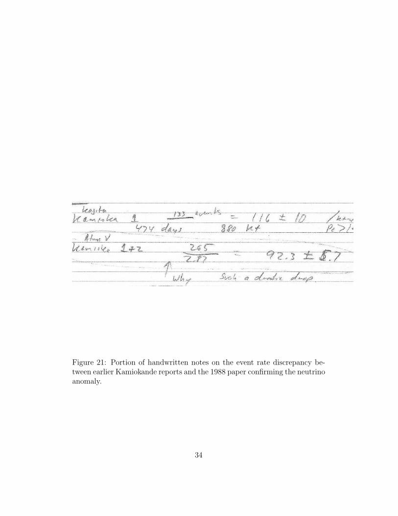
Figure 21: Portion of handwritten notes on the event rate discrepancy be-tween earlier Kamiokande reports and the 1988 paper confirming the neutrinoanomaly.

34

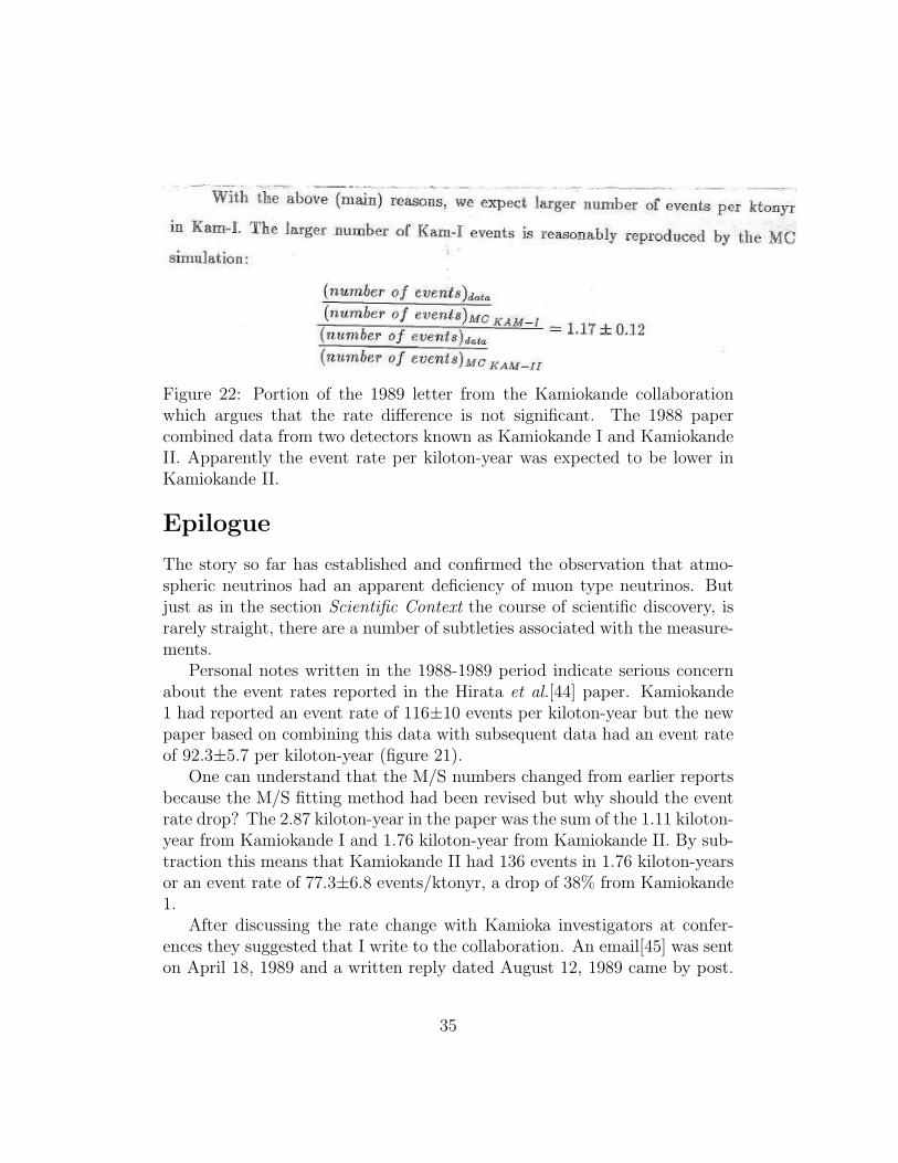
Figure 22: Portion of the 1989 letter from the Kamiokande collaborationwhich argues that the rate difference is not significant. The 1988 papercombined data from two detectors known as Kamiokande I and KamiokandeII. Apparently the event rate per kiloton-year was expected to be lower inKamiokande II.

Epilogue

The story so far has established and confirmed the observation that atmo-spheric neutrinos had an apparent deficiency of muon type neutrinos. Butjust as in the section Scientific Context the course of scientific discovery, israrely straight, there are a number of subtleties associated with the measure-ments.

Personal notes written in the 1988-1989 period indicate serious concernabout the event rates reported in the Hirata et al.[44] paper. Kamiokande1 had reported an event rate of 116±10 events per kiloton-year but the newpaper based on combining this data with subsequent data had an event rateof 92.3±5.7 per kiloton-year (figure 21).

One can understand that the M/S numbers changed from earlier reportsbecause the M/S fitting method had been revised but why should the eventrate drop? The 2.87 kiloton-year in the paper was the sum of the 1.11 kiloton-year from Kamiokande I and 1.76 kiloton-year from Kamiokande II. By sub-traction this means that Kamiokande II had 136 events in 1.76 kiloton-yearsor an event rate of 77.3±6.8 events/ktonyr, a drop of 38% from Kamiokande1.

After discussing the rate change with Kamioka investigators at confer-ences they suggested that I write to the collaboration. An email[45] was senton April 18, 1989 and a written reply dated August 12, 1989 came by post.

35

The response[46] (figure 22) indicated that a refit of Kamiokande I had anevent rate of 116±9.4 events/ktonyr, in good agreement with my estimates.They also indicated that both Kamiokande I and Kamiokande II had ratesin agreement with expectations.

It would have been nice to see the muon neutrino fraction independentlyfor these two exposures, Kamiokande I and II. But the data has never beenreleased in a format that would make that possible.

My notes indicate that a neutrino event rate check was done with theindependent IMB data sample. IMB-1 had an event rate of 106±5 eventper kiloton-year. In the first 1.53 kt-yr of exposure IMB-3 had a rate of110±10 per kiloton-year, for energies above 140 MeV. It would appear thatthe neutrino flux was stable over the period in question.

Conclusions

The author is neither a philosopher nor an historian so readers are encour-aged to draw their own conclusions. Scientific research is a human endeavorcarried out by people with conflicting standards. Scientists are often ex-pected to draw solid conclusions from incomplete data, while maintainingan open mind. Perhaps the best remedy for this conflict is redundancy andcorroboration.

In scientific research the answers are not in the back of the book andNature doesn’t read Physical Review Letters.

Fred Reines, a colleague on much of the work discussed here, formulateda poem to illustrate the challenges of observational science[47] and is knownto have recited it in the context of this research.

Ode to Frustration

If at first you don’t succeed

What did you expect?

Progress would be slow indeed

With nothing to reject.

A false step here, another there

It means you’re really trying

Besides, the struggle up the stair

36

Itself is satisfying.

So labor with your charming quarks

Though endless multiplying

And weigh each lepton, one by one,

And look for baryons dying.

Dimuon pairs, imploding stars

All vie for a solution

With quarks behind their prison bars

Compounding the confusion.

Oh, Pauli, Fermi guide us

Banish our illusions

And elevate our hunches

To sensible conclusions.

It took many years and various kinds of measurements to understand theatmospheric and solar neutrino observations. Over the course of time ourview of the significance of the results has changed. But the story is not over.The neutrino sector still has some discrepant observations that do not fit intothe picture and many parameters needed to finish the picture itself, such asthe overall mass scale, are just starting to be measured.

Acknowledgments

This work would have been impossible without the contributions of manypeople. Larry Sulak, Fred Reines, Maurice Goldhaber and Jack Van derVelde provided the leadership for the IMB experiment, which was in manyways the first large scale experiment in astro-particle physics. Many creativeand hardworking people have contributed. Most have been mentioned inthe article but should also be recognized here. Students Bruce Cortez, BillFoster, Eric Shumard, Geoff Blewitt and Todd Haines all played an impor-tant role. The next generation included Dave Casper, Steve Dye and ClarkMcGrew who helped confirm the result with the IMB-3 data and some new,independent particle classification methods. Richard Bionta was a master atcalibration and designed and constructed the system that converted raw de-tector information into useful physical observations. Tegid W. Jones, Danka

37

Keilczewska and John Learned have provided brilliant independent interpre-tations of the various observations. Many additional members of the IMBcollaboration contributed to its success.

M. Koshiba, Y. Totsuka and T. Kajita have always shown a willingnessto discuss physics even if they did not always share my point of view.

Steve Weinberg, Shelley Glashow, Howard Georgi, Abdus Salam and Jo-gesh Pati provided solid theoretical motivation for the project as well asenthusiastic support.

I would like to thank Allan Franklin for encouragement. In particu-lar, I benefited from many suggestions he made on an early version of thismanuscript.

References

[1] F. Reines, M. F. Crouch, T. L. Jenkins, W. R. Kropp, H. S. Gurr,G. R. Smith J. P. F. Sellschop and B. Meyer, “Evidence for High-Energy Cosmic-Ray Neutrino Interactions”, Phys. Rev. Lett. 15, 429-433 (1965)

[2] Krishnaswamy, M. R.; Menon, M. G. K.; Narasimham, V. S.; Hino-tani, K.; Ito, N.; Miyake, S.; Osborne, J. L.; Parsons, A. J.;Wolfendale, A. W.“The Kolar Gold Fields Neutrino Experiment. II.Atmospheric Muons at a Depth of 7000 hg cm-2 (Kolar)”, Proceedingsof the Royal Society of London. Series A, Mathematical and PhysicalSciences, Volume 323, Issue 1555, pp. 511-522 (1971).

[3] Peter Galison, “How the first neutral-current experiments ended”,Rev. Mod. Phys. 55, 477509 (1983)Andrew Pickering, “Against Putting the Phenomena First: The Dis-covery of the Weak Neutral Current”, Studies in the History andPhilosophy of Science, 15, 85-117 (1984)B. Aubert, A. Benvenuti, D. Cline, W. T. Ford, R. Imlay, T. Y. Ling,A. K. Mann, F. Messing, R. L. Piccioni, J. Pilcher, D. D. Reeder,C. Rubbia, R. Stefanski, and L. Sulak, “ Observation of MuonlessNeutrino-Induced Inelastic Interactions”, Phys. Rev. Lett. 32, 800-803 (1974)

38

[4] B. Aubert, A. Benvenuti, D. Cline, W. T. Ford, R. Imlay, T. Y. Ling,A. K. Mann, F. Messing, J. Pilcher, D. D. Reeder, C. Rubbia, R. Ste-fanski, and L. Sulak, “Scaling-Variable Distributions in High-EnergyInelastic Neutrino Interactions”, Phys. Rev. Lett. 33, 984987 (1974)A. Benvenuti, D. Cline, W. T. Ford, R. Imlay, T. Y. Ling, A. K.Mann, F. Messing, D. D. Reeder, C. Rubbia, R. Stefanski, and L.Sulak, “Invariant-Mass Distributions from Inelastic nu and nu -barInteractions”, Phys. Rev. Lett. 34, 597600 (1975)A. Benvenuti, D. Cline, W. T. Ford, R. Imlay, T. Y. Ling, A. K.Mann, D. D. Reeder, C. Rubbia, R. Stefanski, L. Sulak, and P. Wan-derer, “Further Data on the High-y Anomaly in Inelastic AntineutrinoScattering”, Phys. Rev. Lett. 36, 1478-1482 (1976)

[5] V. A. Lubimov, E. G. Novikov, V. Z. Nozik, E. F. Tretyakov and V. S.Kosik, “An estimate of the e neutrino mass from the Beta-spectrumof tritium in the valine molecule”, Phys. Lett. B94, 266 (1980).

[6] K.E. Bergkvist, Nuclear Physics B39, 839 (1972).

[7] E. Pasierb, H. S. Gurr, J. Lathrop-, F. Reines, and H. W. So-bel, “Detection of Weak Neutral Current Using Fission nu -bare onDeuterons”, Phys. Rev. Lett. 43, 9699 (1979)F. Reines, H. W. Sobel, and E. Pasierb, “Evidence for Neutrino In-stability”, Phys. Rev. Lett. 45, 13071311 (1980).

[8] B. Pontecorvo, Zh. Eksp. Teor. Fiz. 53, 1717 (1967)B. Pontecorvo, Zh. Eksp. Teor. Fiz. 33, 549 (1957)B. Pontecorvo, Zh. Eksp. Teor. Fiz. 34, 247 (1958)V. Gribov and B. Pontecorvo, Phys. Lett. 28B 495 (1969).

[9] Martin L. Perl, “The Discovery of the Tau Lepton and the Changes inElementary-Particle Physics in Forty Years”, Physics in Perspective6 (2004) 401-427.

[10] A. K. Mann and H. Primakoff, “Neutrino oscillations and the numberof neutrino types”, Phys. Rev D15 (1977), 655-665.

[11] M. Kobayashi and T. Maskawa, “CP-Violation in the RenormalizableTheory of Weak Interaction” Progress of Theoretical Physics (Vol. 49No. 2 (1973), pp.652-657)

39

[12] N. Cabibbo, “Unitary Symmetry and Leptonic Decays”,Phys. Rev. Lett. 10 531-533 (1963).

[13] L. Wolfenstein, “Neutrino oscillations in matter”, Phys. Rev. D 17,2369-2374 (1978).

[14] H. David Politzer , “Reliable Perturbative Results for Strong Interac-tions?”, Phys. Rev. Lett. 30, 1346-1349 (1973).David J. Gross and Frank Wilczek, ”Ultraviolet Behavior of Non-Abelian Gauge Theories”, Phys. Rev. Lett. 30, 1343-1346 (1973).

[15] Howard Georgi and S. L. Glashow, “Unity of All Elementary-ParticleForces”, Phys. Rev. Lett. 32, 438441 (1974).

[16] H. Georgi, H. R. Quinn, and S. Weinberg, “Hierarchy of Interactionsin Unified Gauge Theories”, Phys. Rev. Lett. 33, 451-454 (1974).

[17] B. Cortez, “Birth of the Large Scale Imaging Water Cherenkov De-tector” Sulak Festschrift, Boston University, October 22, 2005.

[18] J.M. LoSecco, F. Reines and D. Sinclair, “The Search for ProtonDecay”, Scientific American, 252 pages 54-62, June 1985.

[19] E. Egelman et al., “A Study of the Time Evolution of a Long-Livedνµ Beam”, submitted to Brookhaven National Laboratory, 1977.

[20] M. Goldhaber, W. Kropp, J. Learned, R. March, F. Reines, J. Schultz,D. Sinclair, H. Sobel, L. Sulak, J. Vander Velde, “A Proposal to Testfor Baryon Stability to a Lifetime of 1033 Years”, May 1979.

[21] Bruce Cortez, private communication.

[22] B. Cortez and L. Sulak, in Unification of the Fundamental ParticleInteractions, Proceedings of the Erice Workshop Europhysics Meeting,edited by S. Ferrara, J. Ellis and P. van Nieuwenhuizen March 1980,pages 661-671.

[23] L. Sulak, First Workshop on Grand Unification edited by P.H. Framp-ton, S.L. Glashow and A. Yildiz April 1980, pages 163-188.

[24] R. M. Bionta, H. S. Park, B. Cortez, L. Sulak, “Stopping Muons inthe IMB Detector”, PDK Memo 82-6, April 1, 1982.

40

[25] Bill Foster, “The Making of the 5 Years Neutrino Background Tapes”,PDK Memo 83-103, July 18, 1983.

[26] B. Cortez and G.W. Foster Harvard University PhD. theses 1983.

[27] E. Shumard University of Michigan PhD. thesis 1984.

[28] G. Blewitt California Institute of Technology PhD. thesis 1985.

[29] J. LoSecco, “Physics Results from Underground Experiments”, NewFrontiers in Particle Physics, Proceedings of the Lake Louise WinterSchool edited by J.M. Cameron, B.A. Campbell, A.N. Kamal andF.C. Khanna February 1986 pages 376-392.

[30] G. Battistoni et al., “Nucleon Decay and Atmospheric Neutrinos atthe Mont Blanc Experiment”, Proceedings of the 19’th InternationalCosmic Ray Conference, La Jolla (1985) volume 8 pages 271-274.

[31] M. Koshiba, Talk presented at the 1986 Aspen Winter Conference onParticle Physics 1986.

[32] T. Haines University of California at Irvine PhD. 1986.

[33] T. J. Haines, R. M. Bionta, G. Blewitt, C. B. Bratton, D. Casper,R. Claus, B. G. Cortez, S. Errede, G. W. Foster, W. Gajewski, K. S.Ganezer, M. Goldhaber, T. W. Jones, D. Kielczewska, W. R. Kropp,J. G. Learned, E. Lehmann, J. M. LoSecco, J. Matthews, H. S. Park,L. R. Price, F. Reines, J. Schultz, S. Seidel, E. Shumard, D. Sinclair,H. W. Sobel, J. L. Stone, L. Sulak, R. Svoboda, J. C. van der Velde,and C. Wuest, “Calculation of Atmospheric Neutrino-Induced Back-grounds in a Nucleon-Decay Search”, Phys. Rev. Lett. 57, 1986-1989(1986).

[34] J. M. LoSecco, R. M. Bionta, G. Blewitt, C. B. Bratton, D. Casper, P.Chrysicopoulou, R. Claus, B. G. Cortez, S. Errede, G. W. Foster, W.Gajewski, K. S. Ganezer, M. Goldhaber, T. J. Haines, T. W. Jones,D. Kielczewska, W. R. Kropp, J. G. Learned, E. Lehmann, H. S.Park, F. Reines, J. Schultz, S. Seidel, E. Shumard, D. Sinclair, H. W.Sobel, J. L. Stone, L. Sulak, R. Svoboda, J. C. Vander Velde, and C.Wuest, “A Study of Atmospheric Neutrinos with the IMB Detector”,

41

Proceedings of the 19’th International Cosmic Ray Conference, LaJolla (1985) volume 8 pages 116-119.

[35] J. LoSecco and J. Learned, “Recent Results from IMB”, Proceedingsof the International School on Particles and Cosmology, Baksan Val-ley, USSR, edited by V.A. Matveev, E.N. Alexeev, V.A. Rubikov andI.I Tkachev, pages 91-108 (1991).

[36] J. M. LoSecco, R. M. Bionta, G. Blewitt, C. B. Bratton, D. Casper, R.Claus, B. Cortez, S. Errede, G. Foster, W. Gajewski, K. S. Ganezer,M. Goldhaber, T. J. Haines, T. W. Jones, D. Kielczewska, W. R.Kropp, J. G. Learned, E. Lehmann, H. S. Park, F. Reines, J. Schultz,S. Seidel, E. Shumard, D. Sinclair, H. W. Sobel, J. L. Stone, L. Su-lak, R. Svoboda, J. C. Van der Velde, and C. Wuest, “Limits on theneutrino lifetime”, Phys. Rev. D 35, 2073-2076 (1987).

[37] J. M. LoSecco, “Off-diagonal neutral currents”, Phys. Rev. D 35, 1716-1718 (1987).

[38] J. M. LoSecco, R. M. Bionta, G. Blewitt, C. B. Bratton, D. Casper, P.Chrysicopoulou, R. Claus, B. G. Cortez, S. Errede, G. W. Foster, W.Gajewski, K. S. Ganezer, M. Goldhaber, T. J. Haines, T. W. Jones,D. Kielczewska, W. R. Kropp, J. G. Learned, E. Lehmann, H. S. Park,F. Reines, J. Schultz, S. Seidel, E. Shumard, D. Sinclair, H. W. Sobel,J. L. Stone, L. Sulak, R. Svoboda, J. C. Vander Velde, and C. Wuest,“Test of Neutrino Oscillations Using Atmospheric Neutrinos”, Phys.Rev. Lett. 54, 2299-2301 (1985).

[39] M. Nakahata et al., “Atmospheric neutrino background andpion nuclear effect for Kamioka nucleon decay experiment”,J. Phys. Soc. Japan 55 (1986) 3786.

[40] M. Koshiba, “Results from the Kamioka Nucleon Decay Experiment”Proceedings of the Fifth Workshop on Grand Unification, pages 13-30, edited by K. Kang, H. Fried and P. Frampton (World Scientific,1984).

[41] Katsushi Arisaka, “Experimental Search for Nucleon Decay”, PhDthesis University of Tokyo, January 1985, UTICEPP-85-01.

42

[42] M. Koshiba, “Kamioka Nucleon Decay Experiment”, Proceedings ofthe Sixth Workshop on Grand Unification, pages 65-88, edited byS. Rudaz and T. Walsh (World Scientific 1985).

[43] T. Kajita PhD. thesis Tokyo University 1986. UTICEPP-86-03 Feb.1986.

[44] K.S. Hirata et al., “Experimental study of the atmospheric neutrinoflux”, Phys. Lett. B205,(1988) 416.

[45] J. LoSecco Email to Totsuka April 18, 1989

[46] Y. Totsuka and T. Kajita, letter August 12, 1989.

[47] Fred Reines, private communication, used with permission.

43