Embed Size (px)
Citation preview
THE HITCHHIKER GUIDE TO: SECANT VARIETIES AND TENSORDECOMPOSITION.
ALESSANDRA BERNARDI∗, ENRICO CARLINI∗, MARIA VIRGINIA CATALISANO∗, ALESSANDRO GIMIGLIANO∗,AND ALESSANDRO ONETO∗
∗ The initial elaboration of this work had Anthony V. Geramitaas one of the authors. The paper is dedicated to him.
Abstract. We consider here the problem, which is quite classical in Algebraic geometry, of studying thesecant varieties of a projective variety X. The case we concentrate on is when X is a Veronese variety, aGrassmannian or a Segre variety. Not only these varieties are among the ones that have been most classicallystudied, but a strong motivation in taking them into consideration is the fact that they parameterize, respec-tively, symmetric, skew-symmetric and general tensors, which are decomposable, and their secant varietiesgive a stratification of tensors via tensor rank. We collect here most of the known results and the openproblems on this fascinating subject.
Contents
1. Introduction 21.1. The Classical Problem 21.2. Secant Varieties and Tensor Decomposition 32. Symmetric Tensors and Veronese Varieties 52.1. On Dimensions of Secant Varieties of Veronese Varieties 62.2. Fat Points in the Plane and SHGH Conjecture 192.3. Algorithms for the Symmetric-Rank of a Given Polynomial 303. Tensor Product and Segre Varieties 453.1. Introduction: First Approaches 453.2. The Multiprojective Affine Projective Method 463.3. The Balanced Case 483.4. The General Case 494. Other Structured Tensors 494.1. Exterior Powers and Grassmannians 504.2. Segre–Veronese Varieties 524.3. Tangential and Osculating Varieties to Veronese Varieties 534.4. Chow–Veronese Varieties 554.5. Varieties of Reducible Forms 574.6. Varieties of Powers 585. Beyond Dimensions 60
2010 Mathematics Subject Classification. 13D40, 14A05, 14A10, 14A15, 14C20, 14M12, 14M15, 14M99, 14N05, 15A69,15A75.
Keywords. Additive decompositions; Secant varieties; Veronese varieties; Segre varieties; Segre-Veronese varieties; Grassman-nians; tensor rank; Waring rank; algorithm.
1
arX
iv:1
812.
1026
7v1
[m
ath.
AG
] 2
6 D
ec 2
018
2 A. BERNARDI, E. CARLINI, M.V. CATALISANO, A. GIMIGLIANO, AND A. ONETO
5.1. Maximum Rank 605.2. Bounds on the Rank 615.3. Formulae for Symmetric Ranks 655.4. Identifiability of Tensors 675.5. Varieties of Sums of Powers 685.6. Equations for the Secant Varieties 715.7. The Real World 74References 75
Funding. A.B. acknowledges the Narodowe Centrum Nauki, Warsaw Center of Mathematics and Computer Science, Institute of
Mathematics of university of Warsaw which financed the 36th Autumn School in Algebraic Geometry “Power sum decompositions
and apolarity, a geometric approach” September 1st-7th, 2013 Łukęcin, Poland where a partial version of the present paper was
conceived. M.V. C. and A. G. acknowledges financial support from MIUR (Italy). A.O. acknowledges financial support from the
Spanish Ministry of Economy and Competitiveness, through the Maria de Maeztu Programme for Units of Excellence in R&D
(MDM-2014-0445).
1. Introduction1.1. The Classical Problem. When considering finite dimensional vector spaces over a field k (which forus, will always be algebraically closed and of characteristic zero, unless stated otherwise), there are threemain functors that come to attention when doing multilinear algebra:
• the tensor product, denoted by V1 ⊗ · · · ⊗ Vd;• the symmetric product, denoted by SdV ;• the wedge product, denoted by
∧dV .
These functors are associated with three classically-studied projective varieties in algebraic geometry (seee.g., [1]):
• the Segre variety;• the Veronese variety;• the Grassmannian.
We will address here the problem of studying the higher secant varieties σs(X), where X is one of thevarieties above. We have:
(1.1) σs(X) :=⋃
P1,...,Ps∈X〈P1, . . . , Ps〉
i.e., σs(X) is the Zariski closure of the union of the Ps−1’s, which are s-secant to X.The problem of determining the dimensions of the higher secant varieties of many classically-studied
projective varieties (and also projective varieties in general) is quite classical in algebraic geometry and has along and interesting history. By a simple count of parameters, the expected dimension of σs(X), for X ⊂ PN ,is min{s(dimX) + (s − 1), N}. This is always an upper-bound of the actual dimension, and a variety X issaid to be defective, or s-defective, if there is a value s for which the dimension of σs(X) is strictly smallerthan the expected one; the difference:
δs(X) := min{s(dimX) + (s− 1), N} − dimσs(X)
is called the s-defectivity of X (or of σs(X)); a variety X for which some δs is positive is called defective.
THE HITCHHIKER GUIDE TO: SECANT VARIETIES AND TENSOR DECOMPOSITION. 3
The first interest in the secant variety σ2(X) of a variety X ⊂ PN lies in the fact that if σ2(X) 6= PN ,then the projection of X from a generic point of PN into PN−1 is an isomorphism. This goes back to theXIX Century with the discovery of a surface X ⊂ P5, for which σ2(X) is a hypersurface, even though itsexpected dimension is five. This is the Veronese surface, which is the only surface in P5 with this property.The research on defective varieties has been quite a frequent subject for classical algebraic geometers, e.g.,see the works of F. Palatini [2], A. Terracini [3, 4] and G.Scorza [5, 6].
It was then in the 1990s that two new articles marked a turning point in the study about these questionsand rekindled the interest in these problems, namely the work of F. Zak and the one by J. Alexander and A.Hirshowitz.
Among many other things, like, e.g., proving Hartshorne’s conjecture on linear normality, the outstandingpaper of F. Zak [7] studied Severi varieties, i.e., non-linearly normal smooth n-dimensional subvarietiesX ⊂ PN , with 2
3 (N−1) = n. Zak found that all Severi varieties have defective σ2(X), and, by using invarianttheory, classified all of them as follows.
Theorem 1.1. Over an algebraically-closed field of characteristic zero, each Severi variety is projectivelyequivalent to one of the following four projective varieties:
• Veronese surface ν2(P2) ⊂ P5;• Segre variety ν1,1(P2 × P2) ⊂ P8;• Grassmann variety Gr(1, 5) ⊂ P14;• Cartan variety E16 ⊂ P26.
Moreover, later in the paper, also Scorza varieties are classified, which are maximal with respect to defec-tivity and which generalize the result on Severi varieties.
The other significant work is the one done by J. Alexander and A. Hirschowitz; see [8] and Theorem2.12 below. Although not directly addressed to the study of secant varieties, they confirmed the conjecturethat, apart from the quadratic Veronese varieties and a few well-known exceptions, all the Veronese varietieshave higher secant varieties of the expected dimension. In a sense, this result completed a project that wasunderway for over 100 years (see [2, 3, 9]).
1.2. Secant Varieties and Tensor Decomposition. Tensors are multidimensional arrays of numbers andplay an important role in numerous research areas including computational complexity, signal processing fortelecommunications [10] and scientific data analysis [11]. As specific examples, we can quote the complexity ofmatrix multiplication [12], the P versus NP complexity problem [13], the study of entanglement in quantumphysics [15, 14], matchgates in computer science [13], the study of phylogenetic invariants [16], independentcomponent analysis [17], blind identification in signal processing [18], branching structure in diffusion im-ages [19] and other multilinear data analysis techniques in bioinformatics and spectroscopy [20]. Looking atthis literature shows how knowledge about this subject used to be quite scattered and suffered a bit from thefact that the same type of problem can be considered in different areas using a different language.
In particular, tensor decomposition is nowadays an intensively-studied argument by many algebraic ge-ometers and by more applied communities. Its main problem is the decomposition of a tensor with a givenstructure as a linear combination of decomposable tensors of the same structure called rank-one tensors.To be more precise: let V1, . . . , Vd be k-vector spaces of dimensions n1 + 1, . . . , nd + 1, respectively, and letV = V ∗1 ⊗ · · · ⊗ V ∗d ' (V1 ⊗ . . . ⊗ Vd)∗. We call a decomposable, or rank-one, tensor an element of the typev∗1 ⊗ · · · ⊗ v∗d ∈ V. If T ∈ V , one can ask:
What is the minimal length of an expression of T as a sum of decomposable tensors?
We call such an expression a tensor decomposition of T , and the answer to this question is usually referredto as the tensor rank of T . Note that, since V is a finite-dimensional vector space of dimension
∏di=1 dimk Vi,
4 A. BERNARDI, E. CARLINI, M.V. CATALISANO, A. GIMIGLIANO, AND A. ONETO
which has a basis of decomposable tensors, it is quite trivial to see that every T ∈ V can be written as thesum of finitely many decomposable tensors. Other natural questions to ask are:
What is the rank of a generic tensor in V ? What is the dimension of the closure of the set ofall tensors of tensor rank ¬ r?
Note that it is convenient to work up to scalar multiplication, i.e., in the projective space P(V), andthe latter questions are indeed meant to be considered in the Zariski topology of P(V). This is the naturaltopology used in algebraic geometry, and it is defined such that closed subsets are zero loci of (homogeneous)polynomials and open subsets are always dense. In this terminology, an element of a family is said to begeneric in that family if it lies in a proper Zariski open subset of the family. Hence, saying that a propertyholds for a generic tensor in P(V ) means that it holds on a proper Zariski subset of P(V ).
In the case d = 2, tensors correspond to ordinary matrices, and the notion of tensor rank coincides withthe usual one of the rank of matrices. Hence, the generic rank is the maximum one, and it is the same withrespect to rows or to columns. When considering multidimensional tensors, we can check that in general, allthese usual properties for tensor rank fail to hold; e.g., for (2× 2× 2)-tensors, the generic tensor rank is two,but the maximal one is three, and of course, it cannot be the dimension of the space of “row vectors” inwhatever direction.
It is well known that studying the dimensions of the secant varieties to Segre varieties gives a first ideaof the stratification of V , or equivalently of P(V ), with respect to tensor rank. In fact, the Segre varietyν1,...,1(Pn1 × . . . × Pnd) can be seen as the projective variety in P(V), which parametrizes rank-one tensors,and consequently, the generic point of σs(ν1,...,1(Pn1 × · · · × Pnd)) parametrizes a tensor of tensor rank equalto s (e.g., see [21, 22]).
If V1 = · · · = Vd = V of dimension n+1, one can just consider symmetric or skew-symmetric tensors. In thefirst case, we study the SdV ∗, which corresponds to the space of homogeneous polynomials in n+1 variables.Again, we have a notion of symmetric decomposable tensors, i.e, elements of the type (v∗)d ∈ SdV ∗, whichcorrespond to powers of linear forms. These are parametrized by the Veronese variety νd(Pn) ⊂ P(SdV ∗). Inthe skew-symmetric case, we consider
∧dV ∗, whose skew-symmetric decomposable tensors are the elements
of the form v∗1 ∧ . . . ∧ v∗d ∈∧d
V ∗. These are parametrized by the Grassmannian Gr(d, n+ 1) in its Pluckerembedding. Hence, we get a notion of symmetric-rank and of ∧-rank for which one can ask the same questionsas in the case of arbitrary tensors. Once again, these are translated into algebraic geometry problems on secantvarieties of Veronese varieties and Grassmannians.
Notice that actually, Veronese varieties embedded in a projective space corresponding to P(SdV ∗) canbe thought of as sections of the Segre variety in P((V ∗)⊗d) defined by the (linear) equations given by thesymmetry relations.
Since the case of symmetric tensors is the one that has been classically considered more in depth, due to thefact that symmetric tensors correspond to homogeneous polynomials, we start from analyzing secant varietiesof Veronese varieties in Section 2. Then, we pass to secant varieties of Segre varieties in Section 3. Then, Section4 is dedicated to varieties that parametrize other types of structured tensors, such as Grassmannians, whichparametrize skew-symmetric tensors, Segre–Veronese varieties, which parametrize decomposable partially-symmetric tensors, Chow varieties, which parametrize homogeneous polynomials, which factorize as productof linear forms, varieties of powers, which parametrize homogeneous polynomials, which are pure k-th powersin the space of degree kd, or varieties that parametrize homogeneous polynomials with a certain prescribedfactorization structure. In Section 5, we will consider other problems related to these kinds of questions, e.g.,what is known about maximal ranks, how to find the actual value of (or bounds on) the rank of a given tensor,how to determine the number of minimal decompositions of a tensor, what is known about the equations of
THE HITCHHIKER GUIDE TO: SECANT VARIETIES AND TENSOR DECOMPOSITION. 5
the secant varieties that we are considering or what kind of problems we meet when treating this problemover R, a case that is of course very interesting for applications.
2. Symmetric Tensors and Veronese Varieties
A symmetric tensor T is an element of the space SdV ∗, where V ∗ is an (n + 1)-dimensional k-vectorspace and k is an algebraically-closed field. It is quite immediate to see that we can associate a degree dhomogeneous polynomial in k[x0, . . . , xn] with any symmetric tensor in SdV ∗.
In this section, we address the problem of symmetric tensor decomposition.
What is the smallest integer r such that a given symmetric tensor T ∈ SdV ∗ can be writ-ten as a sum of r symmetric decomposable tensors, i.e., as a sum of r elements of the type(v∗)⊗d ∈ (V ∗)⊗d?
We call the answer to the latter question the symmetric rank of T . Equivalently,
What is the smallest integer r such that a given homogeneous polynomial F ∈ SdV ∗ (a (n+1)-aryd-ic, in classical language) can be written as a sum of r d-th powers of linear forms?
We call the answer to the latter question the Waring rank, or simply rank, of F ; denoted Rsym(F ).Whenever it will be relevant to recall the base field, it will be denoted by Rk
sym(F ). Since, as we havesaid, the space of symmetric tensors of a given format can be naturally seen as the space of homogeneouspolynomials of a certain degree, we will use both names for the rank.
The name “Waring rank” comes from an old problem in number theory regarding expressions of integersas sums of powers; we will explain it in Section 2.1.1.
The first naive remark is that there are(n+dd
)coefficients ai0,··· ,in needed to write:
F =∑
ai0,··· ,inxi00 · · ·xinn ,
and r(n+ 1) coefficients bi,j to write the same F as:
F =r∑i=1
(bi,0x0 + · · ·+ bi,nxn)d.
Therefore, for a general polynomial, the answer to the question should be that r has to be at least such thatr(n+ 1)
(n+dd
). Then, the minimal value for which the previous inequality holds is
⌈1
n+1
(n+dd
)⌉. For n = 2
and d = 2, we know that this bound does not give the correct answer because a regular quadratic form inthree variables cannot be written as a sum of two squares. On the other hand, a straightforward inspectionshows that for binary cubics, i.e., d = 3 and n = 1, the generic rank is as expected. Therefore, the answercannot be too simple.
The most important general result on this problem has been obtained by J. Alexander and A. Hirschowitz,in 1995; see [8]. It says that the generic rank is as expected for forms of degree d 3 in n 1 variablesexcept for a small number of peculiar pairs (n, d); see Theorem 2.12.
What about non-generic forms? As in the case of binary cubics, there are special forms that require alarger r, and these cases are still being investigated. Other presentations of this topic from different pointsof view can be found in [24, 23, 25, 26].
As anticipated in the Introduction, we introduce Veronese varieties, which parametrize homogeneous poly-nomials of symmetric-rank-one, i.e., powers of linear forms; see Section 2.1.2. Then, in order to study thesymmetric-rank of a generic form, we will use the concept of secant varieties as defined in (1.1). In fact, theorder of the first secant that fills the ambient space will give the symmetric-rank of a generic form. The dimen-sions of secant varieties to Veronese varieties were completely classified by J. Alexander and A. Hirschowitz in[8] (Theorem 2.12). We will briefly review their proof since it provides a very important constructive method
6 A. BERNARDI, E. CARLINI, M.V. CATALISANO, A. GIMIGLIANO, AND A. ONETO
to compute dimensions of secant varieties that can be extended also to other kinds of varieties parameterizingdifferent structured tensors. In order to do that, we need to introduce apolarity theory (Section 2.1.4) andthe so-called Horace method (Sections 2.2.1 and 2.2.2).
The second part of this section will be dedicated to a more algorithmic approach to these problems, andwe will focus on the problem of computing the symmetric-rank of a given homogeneous polynomial.
In the particular case of binary forms, there is a very well-known and classical result firstly obtained by J.J. Sylvester in the XIX Century. We will show a more modern reformulation of the same algorithm presentedby G. Comas and M. Seiguer in [27] and a more efficient one presented in [28]; see Section 2.3.1. In Section2.3.2, we will tackle the more general case of the computation of the symmetric-rank of any homogeneouspolynomial, and we will show the only theoretical algorithm (to our knowledge) that is able to do so, whichwas developed by J. Brachat, P. Comon, B. Mourrain and E. Tsigaridas in [30] with its reformulation [32, 31].
The last subsection of this section is dedicated to an overview of open problems.
2.1. On Dimensions of Secant Varieties of Veronese Varieties. This section is entirely devoted tocomputing the symmetric-rank of a generic form, i.e., to the computation of the generic symmetric-rank.As anticipated, we approach the problem by computing dimensions of secant varieties of Veronese varieties.Recall that, in algebraic geometry, we say that a property holds for a generic form of degree d if it holds ona Zariski open, hence dense, subset of P(SdV ∗).
2.1.1. Waring problem for forms. The problem that we are presenting here takes its name from an oldquestion in number theory. In 1770, E. Waring in [9] stated (without proofs) that:
“Every natural number can be written as sum of at most 9 positive cubes, Every natural numbercan be written as sum of at most 19 biquadratics.”
Moreover, he believed that:
“For all integers d 2, there exists a number g(d) such that each positive integer n ∈ Z+ canbe written as sum of the d-th powers of g(d) many positive integers, i.e., n = ad1 + · · · + adg(d)
with ai 0.”
E. Waring’s belief was shown to be true by D. Hilbert in 1909, who proved that such a g(d) indeed existsfor every d 2. In fact, we know from the famous four-squares Lagrange theorem (1770) that g(2) = 4, andmore recently, it has been proven that g(3) = 9 and g(4) = 19. However, the exact number for higher powersis not yet known in general. In [33], H. Davenport proved that any sufficiently large integer can be writtenas a sum of 16 fourth powers. As a consequence, for any integer d 2, a new number G(d) has been defined,as the least number of d-th powers of positive integers to write any sufficiently large positive integer as theirsum. Previously, C. F. Gauss proved that any integer congruent to seven modulo eight can be written as asum of four squares, establishing that G(2) = g(2) = 4. Again, the exact value G(d) for higher powers is notknown in general.
This fascinating problem of number theory was then formulated for homogeneous polynomials as follows.Let k be an algebraically-closed field of characteristic zero. We will work over the projective space Pn = PV
where V is an (n + 1)-dimensional vector space over k. We consider the polynomial ring S = k[x0, . . . , xn]with the graded structure S =
⊕d0 Sd, where Sd = 〈xd0, xd−1
0 x1, . . . , xdn〉 is the vector space of homogeneous
polynomials, or forms, of degree d, which, as we said, can be also seen as the space SdV of symmetrictensors of order d over V . In geometric language, those vector spaces Sd are called complete linear systemsof hypersurfaces of degree d in Pn. Sometimes, we will write PSd in order to mean the projectivization of Sd,namely PSd will be a P(n+dd )−1 whose elements are classes of forms of degree d modulo scalar multiplication,i.e., [F ] ∈ PSd with F ∈ Sd.
THE HITCHHIKER GUIDE TO: SECANT VARIETIES AND TENSOR DECOMPOSITION. 7
In analogy to the Waring problem for integer numbers, the so-called little Waring problem for forms is thefollowing.
Problem 1 (Little Waring problem). Find the minimum s ∈ Z such that all forms F ∈ Sd can be writtenas the sum of at most s d-th powers of linear forms.
The answer to the latter question is analogous to the number g(d) in the Waring problem for integers. Atthe same time, we can define an analogous number G(d), which considers decomposition in sums of powers ofall numbers, but finitely many. In particular, the big Waring problem for forms can be formulated as follows.
Problem 2 (Big Waring problem). Find the minimum s ∈ Z such that the generic form F ∈ Sd can bewritten as a sum of at most s d-th powers of linear forms.
In order to know which elements of Sd can be written as a sum of s d-th powers of linear forms, we studythe image of the map:
(2.1) φd,s : S1 × · · · × S1︸ ︷︷ ︸s
−→ Sd, φd,s(L1, . . . , Ls) = Ld1 + · · ·+ Lds .
In terms of maps φd,s, the little Waring problem (Problem 1) is to find the smallest s, such that Im(φd,s) = Sd.Analogously, to solve the big Waring problem (Problem 2), we require Im(φd,s) = Sd, which is equivalent tofinding the minimal s such that dim(Im(φd,s)) = dimSd.
The map φd,s can be viewed as a polynomial map between affine spaces:
φd,s : As(n+1) −→ AN , with N =(n+ d
n
).
In order to know the dimension of the image of such a map, we look at its differential at a general point Pof the domain:
dφd,s|P : TP (As(n+1)) −→ Tφd,s(P )(AN ).
Let P = (L1, . . . , Ls) ∈ As(n+1) and v = (M1, . . . ,Ms) ∈ TP (As(n+1)) ' As(n+1), where Li,Mi ∈ S1
for i = 1, . . . , s. Let us consider the following parameterizations t 7−→ (L1 + M1t, . . . , Ls + Mst) of a line Cpassing through P whose tangent vector at P is M . The image of C via φd,s is φd,s(L1 +M1t, . . . , Ls+Mst) =∑si=1(Li +Mit)d. The tangent vector to φd,s(C) in φd,s(P ) is:
(2.2)d
dt
∣∣∣∣t=0
(s∑i=1
(Li +Mit)d)
=s∑i=1
d
dt
∣∣∣∣t=0
(Li +Mit)d =s∑i=1
dLd−1i Mi.
Now, as v = (M1, . . . ,Ms) varies in As(n+1), the tangent vectors that we get span 〈Ld−11 S1, . . . , L
d−1s S1〉.
Therefore, we just proved the following.
Proposition 2.1. Let L1, . . . , Ls be linear forms in S = k[x0, . . . , xn], where Li = ai,0x0 + · · ·+ ai,nxn, andconsider the map:
φd,s : S1 × · · · × S1︸ ︷︷ ︸s
−→ Sd, φd,s(L1, . . . , Ls) = Ld1 + · · ·+ Lds ;
then:
rk(dφd,s)|(L1,...,Ls) = dimk〈Ld−11 S1, . . . , L
d−1s S1〉.
It is very interesting to see how the problem of determining the latter dimension has been solved, becausethe solution involves many algebraic and geometric tools.
8 A. BERNARDI, E. CARLINI, M.V. CATALISANO, A. GIMIGLIANO, AND A. ONETO
2.1.2. Veronese Varieties. The first geometric objects that are related to our problem are the Veronesevarieties. We recall that a Veronese variety can be viewed as (is projectively equivalent to) the image ofthe following d-pleembedding of Pn, where all degree d monomials in n+ 1 variables appear in lexicographicorder:
(2.3)νd : Pn ↪→ P(n+dd )−1
[u0 : . . . : un] 7→ [ud0 : ud−10 u1 : ud−1
0 u2 : . . . : udn].
With a slight abuse of notation, we can describe the Veronese map as follows:
(2.4)νd : PS1 = (Pn)∗ ↪→ PSd =
(P(n+dd )−1
)∗[L] 7→ [Ld]
.
Let Xn,d := νd(Pn) denote a Veronese variety.Clearly, “νd as defined in (2.3)” and “νd as defined in (2.4)” are not the same map; indeed, from (2.4),
νd([L]) = νd ([u0x0 + · · ·+ unxn]) = [Ld] =
=[ud0 : dud−1
0 u1 :(d
2
)ud−1
0 u2 : . . . : udn
]∈ PSd.
However, the two images are projectively equivalent. In order to see that, it is enough to consider the monomialbasis of Sd given by: {(
d
α
)xα | α = (α0, . . . , αn) ∈ Nn+1, |α| = d
}.
Given a set of variables x0, . . . , xn, we let xα denote the monomial xα00 · · ·xαnn , for any α ∈ Nn+1. Moreover,we write |α| = α0 + . . .+ αn for its degree. Furthermore, if |α| = d, we use the standard notation
(dα
)for the
multi-nomial coefficient d!α0!···αn! .
Therefore, we can view the Veronese variety either as the variety that parametrizes d-th powers of linearforms or as the one parameterizing completely decomposable symmetric tensors.
Example 2.2 (Twisted cubic). Let V = k2 and d = 3, then:
ν3 : P1 ↪→ P3
[a0 : a1] 7→ [a30 : a2
0a1 : a0a21 : a3
1].
If we take {z0, . . . , z3} to be homogeneous coordinates in P3, then the Veronese curve in P3 (classically knownas twisted cubic) is given by the solutions of the following system of equations:
z0z2 − z21 = 0
z0z3 − z1z2 = 0z1z3 − z2
2 = 0.
Observe that those equations can be obtained as the vanishing of all the maximal minors of the followingmatrix:
(2.5)
(z0 z1 z2
z1 z2 z3
).
Notice that the matrix (2.5) can be obtained also as the defining matrix of the linear map:
S2V ∗ → S1V, ∂2xi 7→ ∂2
xi(F )
where F =∑3i=0
(di
)−1zix
3−i0 xi1 and ∂xi := ∂
∂xi.
Another equivalent way to obtain (2.5) is to use the so-called flattenings. We give here an intuitive ideaabout flattenings, which works only for this specific example.
THE HITCHHIKER GUIDE TO: SECANT VARIETIES AND TENSOR DECOMPOSITION. 9
Write the 2×2×2 tensor by putting in position ijk the variable zi+j+k. This is an element of V ∗⊗V ∗⊗V ∗.There is an obvious isomorphism among the space of 2× 2× 2 tensors V ∗ ⊗ V ∗ ⊗ V ∗ and the space of 4× 2matrices (V ∗⊗ V ∗)⊗ V ∗. Intuitively, this can be done by slicing the 2× 2× 2 tensor, keeping fixed the thirdindex. This is one of the three obvious possible flattenings of a 2 × 2 × 2 tensor: the other two flatteningsare obtained by considering as fixed the first or the second index. Now, after having written all the possiblethree flattenings of the tensor, one could remove the redundant repeated columns and compute all maximalminors of the three matrices obtained by this process, and they will give the same ideal.
The phenomenon described in Example 2.2 is a general fact. Indeed, Veronese varieties are always definedby 2× 2 minors of matrices constructed as (2.5), which are usually called catalecticant matrices.
Definition 2.3. Let F ∈ Sd be a homogeneous polynomial of degree d in the polynomial ring S =k[x0, . . . , xn]. For any i = 0, . . . , d, the (i, d − i)-th catalecticant matrix associated to F is the matrix repre-senting the following linear maps in the standard monomial basis, i.e.,
Cati,d−i(F ) : S∗i −→ Sd−i,
∂ixα 7→ ∂ixα(F ),
where, for any α ∈ Nn+1 with |α| = d− i, we denote ∂d−ixα := ∂d−i
∂xα00 ···∂x
αnn
.
Let {zα | α ∈ Nn+1, |α| = d} be the set of coordinates on PSdV , where V is (n + 1)-dimensional. The(i, d − i)-th catalecticant matrix of V is the
(n+in
)×(n+d−in
)matrix whose rows are labeled by Bi = {β ∈
Nn+1 | |β| = i} and columns are labeled by Bd−i = {β ∈ Nn+1 | |β| = d− i}, given by:
Cati,d−i(V ) =(zβ1+β2
)β1∈Biβ2∈Bd−i
.
Remark 2.4. Clearly, the catalecticant matrix representing Catd−i,i(F ) is the transpose of Cati,d−i(F ).Moreover, the most possible square catalecticant matrix is Catbd/2c,dd/2e(F ) (and its transpose).
Let us describe briefly how to compute the ideal of any Veronese variety.
Definition 2.5. A hypermatrix A = (ai1,...,id)0¬ij¬n, j=1,...,d is said to be symmetric, or completely sym-metric, if ai1,...,id = aiσ(1),...,iσ(d) for all σ ∈ Sd, where Sd is the permutation group of {1, . . . , d}.
Definition 2.6. Let H ⊂ V ⊗d be the(n+dd
)-dimensional subspace of completely symmetric tensors of V ⊗d,
i.e., H is isomorphic to the symmetric algebra SdV or the space of homogeneous polynomials of degree d inn + 1 variables. Let S be a ring of coordinates of P(n+dd )−1 = PH obtained as the quotient S = S/I whereS = k[xi1,...,id ]0¬ij¬n, j=1,...,d and I is the ideal generated by all:
xi1,...,id − xiσ(1),...,iσ(d) ,∀ σ ∈ Sd.
The hypermatrix (xi1,...,id)0¬ij¬n, j=1,...,d, whose entries are the generators of S, is said to be a genericsymmetric hypermatrix .
Let A = (xi1,...,id)0¬ij¬n, j=1,...,d be a generic symmetric hypermatrix, then it is a known result thatthe ideal of any Veronese variety is generated in degree two by the 2 × 2 minors of a generic symmetrichypermatrix, i.e.,
(2.6) I(νd(Pn)) = I2(A) := (2× 2 minors of A) ⊂ S.
See [34] for the set theoretical point of view. In [35], the author proved that the ideal of the Veronese varietyis generated by the two-minors of a particular catalecticant matrix. In his PhD thesis [36], A. Parolin showedthat the ideal generated by the two-minors of that catalecticant matrix is actually I2(A), where A is a genericsymmetric hypermatrix.
10 A. BERNARDI, E. CARLINI, M.V. CATALISANO, A. GIMIGLIANO, AND A. ONETO
2.1.3. Secant Varieties. Now, we recall the basics on secant varieties.
Definition 2.7. Let X ⊂ PN be a projective variety of dimension n. We define the s-th secant variety σs(X)of X as the closure of the union of all linear spaces spanned by s points lying on X, i.e.,
σs(X) :=⋃
P1,...,Ps∈X〈P1, . . . , Ps〉 ⊂ PN .
For any F ⊂ Pn, 〈F〉 denotes the linear span of F , i.e., the smallest projective linear space containing F .
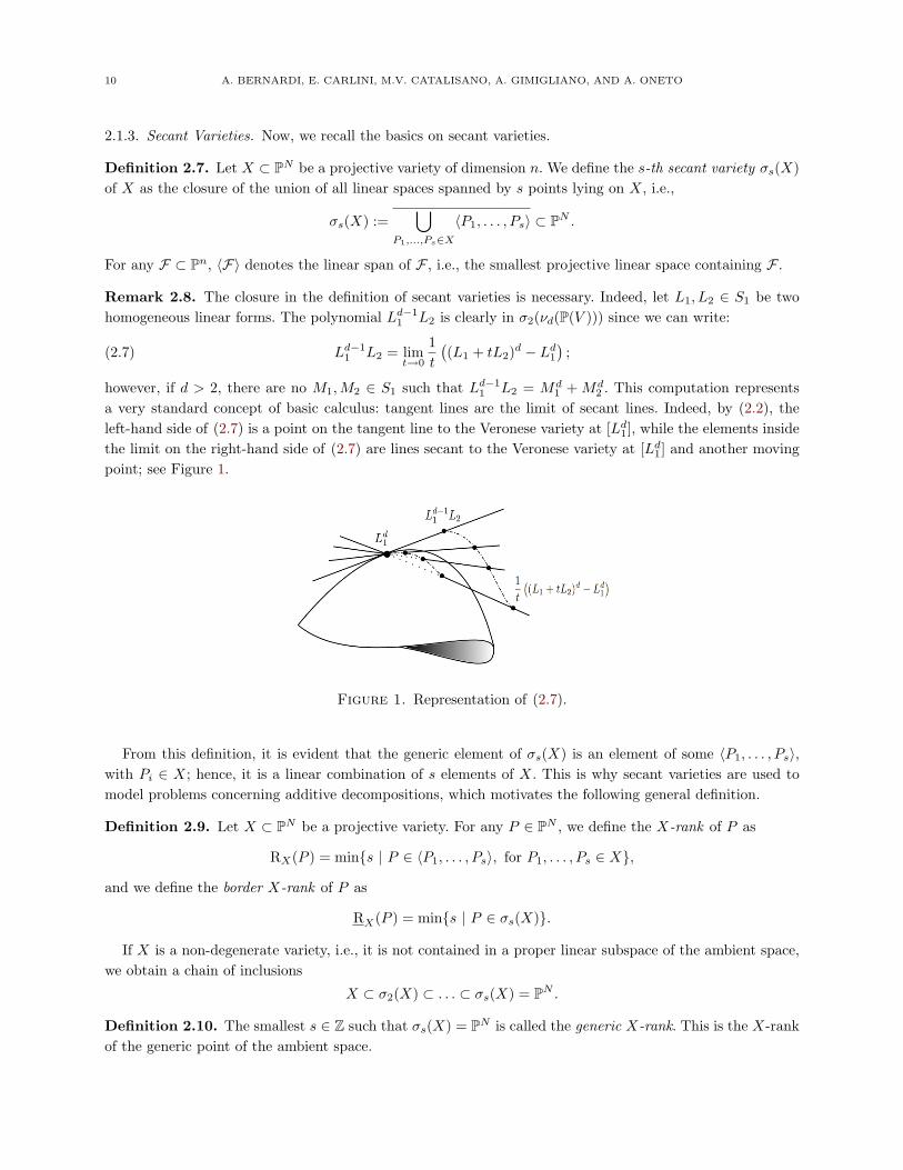
Remark 2.8. The closure in the definition of secant varieties is necessary. Indeed, let L1, L2 ∈ S1 be twohomogeneous linear forms. The polynomial Ld−1
1 L2 is clearly in σ2(νd(P(V ))) since we can write:
(2.7) Ld−11 L2 = lim
t→0
1t
((L1 + tL2)d − Ld1
);
however, if d > 2, there are no M1,M2 ∈ S1 such that Ld−11 L2 = Md
1 + Md2 . This computation represents
a very standard concept of basic calculus: tangent lines are the limit of secant lines. Indeed, by (2.2), theleft-hand side of (2.7) is a point on the tangent line to the Veronese variety at [Ld1], while the elements insidethe limit on the right-hand side of (2.7) are lines secant to the Veronese variety at [Ld1] and another movingpoint; see Figure 1.
Figure 1. Representation of (2.7).
From this definition, it is evident that the generic element of σs(X) is an element of some 〈P1, . . . , Ps〉,with Pi ∈ X; hence, it is a linear combination of s elements of X. This is why secant varieties are used tomodel problems concerning additive decompositions, which motivates the following general definition.
Definition 2.9. Let X ⊂ PN be a projective variety. For any P ∈ PN , we define the X-rank of P as
RX(P ) = min{s | P ∈ 〈P1, . . . , Ps〉, for P1, . . . , Ps ∈ X},
and we define the border X-rank of P as
RX(P ) = min{s | P ∈ σs(X)}.
If X is a non-degenerate variety, i.e., it is not contained in a proper linear subspace of the ambient space,we obtain a chain of inclusions
X ⊂ σ2(X) ⊂ . . . ⊂ σs(X) = PN .
Definition 2.10. The smallest s ∈ Z such that σs(X) = PN is called the generic X-rank. This is the X-rankof the generic point of the ambient space.
THE HITCHHIKER GUIDE TO: SECANT VARIETIES AND TENSOR DECOMPOSITION. 11
The generic X-rank of X is an invariant of the embedded variety X.As we described in (2.4), the image of the d-uple Veronese embedding of Pn = PS1 can be viewed as the
subvariety of PSd made by all forms, which can be written as d-th powers of linear forms. From this point ofview, the generic rank s of the Veronese variety is the minimum integer such that the generic form of degreed in n+ 1 variables can be written as a sum of s powers of linear forms. In other words,
the answer to the Big Waring problem (Problem 2) is the generic rank with respect to the d-upleVeronese embedding in PSd.
This is the reason why we want to study the problem of determining the dimension of s-th secant varietiesof an n-dimensional projective variety X ⊂ PN .
Let Xs := X × · · · ×X︸ ︷︷ ︸s
, X0 ⊂ X be the open subset of regular points of X and:
Us(X) :={
(P1, . . . , Ps) ∈ Xs | ∀ i, Pi∈X0, andthe Pi’s are independent
}.
Therefore, for all (P1, . . . , Ps) ∈ Us(X), since the Pi’s are linearly independent, the linear span H =〈P1, . . . , Ps〉 is a Ps−1. Consider the following incidence variety:
Is(X) = {(Q,H) ∈ PN × Us(X) | Q ∈ H}.
If s ¬ N + 1, the dimension of that incidence variety is:
dim(Is(X)) = n(s− 1) + n+ s− 1.
With this definition, we can consider the projection on the first factor:
π1 : Is(X)→ PN ;
the s-th secant variety of X is just the closure of the image of this map, i.e.,
σs(X) = Im(π1 : Is(X)→ PN ).
Now, if dim(X) = n, it is clear that, while dim(Is(X)) = ns+ s− 1, the dimension of σs(X) can be smaller:it suffices that the generic fiber of π1 has positive dimension to impose dim(σs(X)) < n(s − 1) + n + s − 1.Therefore, it is a general fact that, if X ⊂ PN and dim(X) = n, then,
dim(σs(X)) ¬ min{N, sn+ s− 1}.
Definition 2.11. A projective variety X ⊂ PN of dimension n is said to be s-defective if dim(σs(X)) <min{N, sn+ s− 1}. If so, we call s-th defect of X the difference:
δs(X) := min{N, sn+ s− 1} − dim(σs(X)).
Moreover, if X is s-defective, then σs(X) is said to be defective. If σs(X) is not defective, i.e., δs(X) = 0,then it is said to be regular or of expected dimension.
Alexander–Hirschowitz Theorem ([8]) tells us that the dimension of the s-th secant varieties to Veronesevarieties is not always the expected one; moreover, they exhibit the list of all the defective cases.
Theorem 2.12 (Alexander–Hirschowitz Theorem). Let Xn,d = νd(Pn), for d 2, be a Veronese variety.Then:
dim(σs(X)) = min{(
n+ d
d
)− 1, sn+ s− 1
}except for the following cases:
(1) d = 2, n 2, s ¬ n, where dim(σs(X)) = min{(n+2
2
)− 1, 2n+ 1−
(s2
)};
(2) d = 3, n = 4, s = 7, where δs = 1;
12 A. BERNARDI, E. CARLINI, M.V. CATALISANO, A. GIMIGLIANO, AND A. ONETO
(3) d = 4, n = 2, s = 5, where δs = 1;(4) d = 4, n = 3, s = 9, where δs = 1;(5) d = 4, n = 4, s = 14, where δs = 1.
Due to the importance of this theorem, we firstly give a historical review, then we will give the main stepsof the idea of the proof. For this purpose, we will need to introduce many mathematical tools (apolarity inSection 2.1.4 and fat points together with the Horace method in Section 2.2) and some other excursuses on avery interesting and famous conjecture (the so-called SHGHconjecture; see Conjecture 2.34 and Conjecture2.35) related to the techniques used in the proof of this theorem.
The following historical review can also be found in [37].The quadric cases (d = 2) are classical. The first non-trivial exceptional case d = 4 and n = 2 was
known already by Clebsch in 1860 [38]. He thought of the quartic as a quadric of quadrics and found thatσ5(ν4(P2)) ( P14, whose dimension was not the expected one. Moreover, he found the condition that theelements of σ5(ν4(P2)) have to satisfy, i.e., he found the equation of the hypersurface σ5(ν4(P2)) ( P14: thatcondition was the vanishing of a 6× 6 determinant of a certain catalecticant matrix.
To our knowledge, the first list of all exceptional cases was described by Richmond in [39], who showed allthe defectivities, case by case, without finding any general method to describe all of them. It is remarkablethat he could describe also the most difficult case of general quartics of P4. The same problem, but from amore geometric point of view, was at the same time studied and solved by Palatini in 1902–1903; see [40, 41].In particular, Palatini studied the general problem, proved the defectivity of the space of cubics in P4 andstudied the case of n = 2. He was also able to list all the defective cases.
The first work where the problem was treated in general is due to Campbell (in 1891; therefore, his workpreceded those of Palatini, but in Palatini’s papers, there is no evidence of knowledge of Campbell’s work),who in [42], found almost all the defective cases (except the last one) with very interesting, but not alwayscorrect arguments (the fact that the Campbell argument was wrong for n = 3 was claimed also in [4] in1915).
His approach is very close to the infinitesimal one of Terracini, who introduced in [3] a very simple andelegant argument (today known as Terracini’s lemmas, the first of which will be displayed here as Lemma2.13), which offered a completely new point of view in the field. Terracini showed again the case of n = 2in [3]. In [43], he proved that the exceptional case of cubics in P4 can be solved by considering that therational quartic through seven given points in P4 is the singular locus of its secant variety, which is a cubichypersurface. In [4], Terracini finally proved the case n = 3 (in 2001, Roe, Zappala and Baggio revisedTerracini’s argument, and they where able to present a rigorous proof for the case n = 3; see [44]).
In 1931, Bronowski [45] tried to tackle the problem checking if a linear system has a vanishing Jacobianby a numerical criterion, but his argument was incomplete.
In 1985, Hirschowitz ([46]) proved again the cases n = 2, 3, and he introduced for the first time in the studyof this problem the use of zero-dimensional schemes, which is the key point towards a complete solution ofthe problem (this will be the idea that we will follow in these notes). Alexander used this new and powerfulidea of Hirschowitz, and in [47], he proved the theorem for d 5.
Finally, in [48, 8] (1992–1995), J. Alexander and A. Hirschowitz joined forces to complete the proof ofTheorem 2.12. After this result, simplifications of the proof followed [49, 50].
After this historical excursus, we can now review the main steps of the proof of the Alexander–Hirschowitztheorem. As already mentioned, one of the main ingredients to prove is Terracini’s lemma (see [3] or [51]),which gives an extremely powerful technique to compute the dimension of any secant variety.
Lemma 2.13 (Terracini’s Lemma). Let X be an irreducible non-degenerate variety in PN , and let P1, . . . , Psbe s generic points on X. Then, the tangent space to σs(X) at a generic point Q ∈ 〈P1, . . . , Ps〉 is the linear
THE HITCHHIKER GUIDE TO: SECANT VARIETIES AND TENSOR DECOMPOSITION. 13
span in PN of the tangent spaces TPi(X) to X at Pi, i = 1, . . . , s, i.e.,
TQ(σs(X)) = 〈TP1(X), . . . , TPs(X)〉.
This “lemma” (we believe it is very reductive to call it a “lemma”) can be proven in many ways (forexample, without any assumption on the characteristic of k, or following Zak’s book [7]). Here, we present aproof “made by hand”.
Proof. We give this proof in the case of k = C, even though it works in general for any algebraically-closedfield of characteristic zero.
We have already used the notation Xs for X × · · · ×X taken s times. Suppose that dim(X) = n. Let usconsider the following incidence variety,
I ={
(P ;P1, . . . , Ps) ∈ PN ×Xs∣∣∣ P ∈ 〈P1, . . . , Ps〉
P1, . . . , Ps ∈ X}⊂ PN ×Xs,
and the two following projections,
π1 : I→ σs(X) , π2 : I→ Xs.
The dimension of Xs is clearly sn. If (P1, . . . , Ps) ∈ Xs, the fiber π−12 ((P1, . . . , Ps)) is generically a Ps−1,
s < N . Then, dim(I) = sn+ s− 1.If the generic fiber of π1 is finite, then σs(X) is regular. i.e., it has the expected dimension; otherwise, it
is defective with a value of the defect that is exactly the dimension of the generic fiber.Let (P1, . . . , Ps) ∈ Xs and suppose that each Pi ∈ X ⊂ PN has coordinates Pi = [ai,0 : . . . : ai,N ], for
i = 1, . . . , s. In an affine neighborhood Ui of Pi, for any i, the variety X can be locally parametrized withsome rational functions fi,j : kn+1 → k, with j = 0, . . . , N , that are zero at the origin. Hence, we write:
X ⊃ Ui :
x0 = ai,0 + fi,0(ui,0, . . . , ui,n)
...xN = ai,N + fi,N (ui,0, . . . , ui,n)
.
Now, we need a parametrization ϕ for σs(X). Consider the subspace spanned by s points of X, i.e.,
〈(a1,0 + f1,0, . . . , a1,N + f1,N ), . . . , (as,0 + fs,0, . . . , as,N + fs,N )〉,
where for simplicity of notation, we omit the dependence of the fi,j on the variables ui,j ; thus, an element ofthis subspace is of the form:
λ1(a1,0 + f1,0, . . . , a1,N + f1,N ) + · · ·+ λs(as,0 + fs,0, . . . , as,N + fs,N ),
for some λ1, . . . , λs ∈ k. We can assume λ1 = 1. Therefore, a parametrization of the s-th secant variety to Xin an affine neighborhood of the point P1 + λ2P2 + . . .+ λsPs is given by:
(a1,0 + f1,0, . . . ,a1,N + f1,N )+
+ (λ2 + t2)(a2,1 − a1,0 + f2,1 − f1,0, . . . , a2,N − a1,N + f2,N − f1,N )+
+ · · ·+
+ (λs + ts)(as,1 − a1,0 + fs,1 − f1,0, . . . , as,N − a1,N + fs,N − f1,N ),
for some parameters t2, . . . , ts. Therefore, in coordinates, the parametrization of σs(X) that we are lookingfor is the map ϕ : ks(n+1)+s−1 → kN+1 given by:
(u1,0, . . . , u1,n, u2,0, . . . , u2,n, . . . , us,0, . . . , us,n, t2, . . . , ts)7→
(. . . , a1,j + f1,j + (λ2 + t2)(a2,j − a1,j + f2,j − f1,j) + · · ·+ (λs + ts)(as,j − a1,j + fs,j − f1,j), . . .),
14 A. BERNARDI, E. CARLINI, M.V. CATALISANO, A. GIMIGLIANO, AND A. ONETO
where for simplicity, we have written only the j-th element of the image. Therefore, we are able to writethe Jacobian of ϕ. We are writing it in three blocks: the first one is (N + 1) × (n + 1); the second one is(N + 1)× (s− 1)(n+ 1); and the third one is (N + 1)× (s− 1):
J0(ϕ) =(
(1− λ2 − · · · − λs) ∂f1,j∂u1,k
∣∣∣ λi∂fi,j∂ui,k
∣∣∣ ai,j − a1,j
),
with i = 2, . . . , s; j = 0, . . . , N and k = 0, . . . , n. Now, the first block is a basis of the (affine) tangent spaceto X at P1, and in the second block, we can find the bases for the tangent spaces to X at P2, . . . , Ps; therows of:
∂fi,0∂ui,0
· · · ∂fi,0∂ai,N
......
∂fi,N∂ai,0
· · · ∂fi,N∂ai,N
give a basis for the (affine) tangent space of X at Pi. �
The importance of Terracini’s lemma to compute the dimension of any secant variety is extremely evident.One of the main ideas of Alexander and Hirshowitz in order to tackle the specific case of Veronese variety wasto take advantage of the fact that Veronese varieties are embedded in the projective space of homogeneouspolynomials. They firstly moved the problem from computing the dimension of a vector space (the tangentspace to a secant variety) to the computation of the dimension of its dual (see Section 2.1.4 for the precisenotion of duality used in this context). Secondly, their punchline was to identify such a dual space witha certain degree part of a zero-dimensional scheme, whose Hilbert function can be computed by induction(almost always). We will be more clear on the whole technique in the sequel. Now we need to use the languageof schemes.
Remark 2.14. Schemes are locally-ringed spaces isomorphic to the spectrum of a commutative ring. Ofcourse, this is not the right place to give a complete introduction to schemes. The reader interested instudying schemes can find the fundamental material in [52, 53, 54]. In any case, it is worth noting that wewill always use only zero-dimensional schemes, i.e., “points”; therefore, for our purpose, it is sufficient tothink of zero-dimensional schemes as points with a certain structure given by the vanishing of the polynomialequations appearing in the defining ideal. For example, a homogeneous ideal I contained in k[x, y, z], whichis defined by the forms vanishing on a degree d plane curve C and on a tangent line to C at one of its smoothpoints P , represents a zero-dimensional subscheme of the plane supported at P and of length two, since thedegree of intersection among the curve and the tangent line is two at P (schemes of this kind are sometimescalled jets).
Definition 2.15. A fat point Z ⊂ Pn is a zero-dimensional scheme, whose defining ideal is of the form℘m, where ℘ is the ideal of a simple point and m is a positive integer. In this case, we also say that Zis a m-fat point, and we usually denote it as mP . We call the scheme of fat points a union of fat pointsm1P1 + · · · + msPs, i.e., the zero-dimensional scheme defined by the ideal ℘m11 ∩ · · · ∩ ℘mss , where ℘i is theprime ideal defining the point Pi, and the mi’s are positive integers.
Remark 2.16. In the same notation as the latter definition, it is easy to show that F ∈ ℘m if and only if∂(F )(P ) = 0, for any partial differential ∂ of order ¬ m−1. In other words, the hypersurfaces “vanishing” atthe m-fat point mP are the hypersurfaces that are passing through P with multiplicity m, i.e., are singularat P of order m.
Corollary 2.17. Let (X,L) be an integral, polarized scheme. If L embeds X as a closed scheme in PN , then:
dim(σs(X)) = N − dim(h0(IZ,X ⊗ L)),
THE HITCHHIKER GUIDE TO: SECANT VARIETIES AND TENSOR DECOMPOSITION. 15
where Z is the union of sgeneric two-fat points in X.
Proof. By Terracini’s lemma, we have that, for generic points P1, . . . , Ps ∈ X,
dim(σs(X)) = dim(〈TP1(X), . . . , TPs(X)〉).
Since X is embedded in P(H0(X,L)∗) of dimension N , we can view the elements of H0(X,L) as hyperplanesin PN . The hyperplanes that contain a space TPi(X) correspond to elements in H0(I2Pi,X ⊗ L), since theyintersect X in a subscheme containing the first infinitesimal neighborhood of Pi. Hence, the hyperplanes ofPN containing 〈TP1(X), . . . , TPs(X)〉 are the sections of H0(IZ,X ⊗ L), where Z is the scheme union of thefirst infinitesimal neighborhoods in X of the points Pi’s. �
Remark 2.18. A hyperplane H contains the tangent space to a non-degenerate projective variety X at asmooth point P if and only if the intersection X ∩H has a singular point at P . In fact, the tangent spaceTP (X) to X at P has the same dimension of X and TP (X ∩ H) = H ∩ TP (X). Moreover, P is singularin H ∩ X if and only if dim(TP (X ∩ H)) dim(X ∩ H) = dim(X) − 1, and this happens if and only ifH ⊃ TP (X).
Example 2.19 (The Veronese surface of P5 is defective). Consider the Veronese surface X2,2 = ν2(P2) inP5. We want to show that it is two-defective, with δ2 = 1. In other words, since the expected dimension ofσ2(X2,2) is 2 · 2 + 1, i.e., we expect that σ2(X2,2) fills the ambient space, we want to prove that it is actuallya hypersurface. This will imply that actually, it is not possible to write a generic ternary quadric as a sum oftwo squares, as expected by counting parameters, but at least three squares are necessary instead.
Let P be a general point on the linear span 〈R,Q〉 of two general points R,Q ∈ X; hence, P ∈ σ2(X2,2).By Terracini’s lemma, TP (σ2(X2,2)) = 〈TR(X2,2), TQ(X2,2)〉. The expected dimension for σ2(X2,2) is five,so dim(TP (σ2(X2,2))) < 5 if and only if there exists a hyperplane H containing TP (σ2(X2,2)). The previousremark tells us that this happens if and only if there exists a hyperplane H such that H ∩X2,2 is singularat R,Q. Now, X2,2 is the image of P2 via the map defined by the complete linear system of quadrics; hence,X2,2 ∩H is the image of a plane conic. Let R′, Q′ be the pre-images via ν2 of R,Q respectively. Then, thedouble line defined by R′, Q′ is a conic, which is singular at R′, Q′. Since the double line 〈R′, Q′〉 is the onlyplane conic that is singular at R′, Q′, we can say that dim(TP (σ2(X2,2))) = 4 < 5; hence, σ2(X2,2) is defectivewith defect equal to zero.
Since the two-Veronese surface is defined by the complete linear system of quadrics, Corollary 2.17 allowsus to rephrase the defectivity of σ2(X2,2) in terms of the number of conditions imposed by two-fat points toforms of degree two; i.e., we say that
two two-fat points of P2 do not impose independent conditions on ternary quadrics.As we have recalled above, imposing the vanishing at the two-fat point means to impose the annihilation of
all partial derivatives of first order. In P2, these are three linear conditions on the space of quadrics. Since weare considering a scheme of two two-fat points, we have six linear conditions to impose on the six-dimensionallinear space of ternary quadrics; in this sense, we expect to have no plane cubic passing through two two-fatpoints. However, since the double line is a conic passing doubly thorough the two two-fat points, we havethat the six linear conditions are not independent. We will come back in the next sections on this relationbetween the conditions imposed by a scheme of fat points and the defectiveness of secant varieties.
Corollary 2.17 can be generalized to non-complete linear systems on X.
Remark 2.20. Let D be any divisor of an irreducible projective variety X. With |D|, we indicate thecomplete linear system defined by D. Let V ⊂ |D| be a linear system. We use the notation:
V (m1P1, . . . ,msPs)
16 A. BERNARDI, E. CARLINI, M.V. CATALISANO, A. GIMIGLIANO, AND A. ONETO
for the subsystem of divisors of V passing through the fixed points P1, . . . , Ps with multiplicities at leastm1, . . . ,ms respectively.
When the multiplicities mi are equal to two, for i = 1, . . . , s, since a two-fat point in Pn gives n+ 1 linearconditions, in general, we expect that, if dim(X) = n, then:
exp.dim(V (2P1, . . . , 2Ps)) = dim(V )− s(n+ 1).
Suppose that V is associated with a morphism ϕV : X0 → Pr (if dim(V ) = r), which is an embedding on adense open set X0 ⊂ X. We will consider the variety ϕV (X0).
The problem of computing dim(V (2P1, . . . , 2Ps)) is equivalent to that one of computing the dimension ofthe s-th secant variety to ϕV (X0).
Proposition 2.21. Let X be an integral scheme and V be a linear system on X such that the rational functionϕV : X 99K Pr associated with V is an embedding on a dense open subset X0 of X. Then, σs
(ϕV (X0)
)is
defective if and only if for general points, we have P1, . . . , Ps ∈ X:
dim(V (2P1, . . . , 2Ps)) > min{−1, r − s(n+ 1)}.
This statement can be reformulated via apolarity, as we will see in the next section.
2.1.4. Apolarity. This section is an exposition of inverse systems techniques, and it follows [55].As already anticipated at the end of the proof of Terracini’s lemma, the whole Alexander and Hirshowitz
technique to compute the dimensions of secant varieties of Veronese varieties is based on the computation ofthe dual space to the tangent space to σs(νd(Pn)) at a generic point. Such a duality is the apolarity actionthat we are going to define.
Definition 2.22 (Apolarity action). Let S = k[x0, . . . , xn] and R = k[y0, . . . , yn] be polynomial rings andconsider the action of R1 on S1 and of R1 on S1 defined by:
yi ◦ xj =(
∂
∂xi
)(xj) =
{0, if i 6= j
1, if i = j;
i.e., we view the polynomials of R1 as “partial derivative operators” on S1.
Now, we extend this action to the whole rings R and S by linearity and using properties of differentiation.Hence, we get the apolarity action:
◦ : Ri × Sj −→ Sj−i
where:
yα ◦ xβ =
∏ni=1
(βi)!(βi−αi)!x
β−α, if α ¬ β;
0, otherwise.
for α, β ∈ Nn+1, α = (α0, ..., αn), β = (β0, . . . , βn), where we use the notation α ¬ β if and only if ai ¬ bi forall i = 0, . . . , n, which is equivalent to the condition that xα divides xβ in S.
Remark 2.23. Here, are some basic remarks on apolarity action:
• the apolar action of R on S makes S a (non-finitely generated) R-module (but the converse is nottrue);
• the apolar action of R on S lowers the degree; in particular, given F ∈ Sd, the (i, d−i)-th catalecticantmatrix (see Definition 2.3) is the matrix of the following linear map induced by the apolar action
Cati,d−i(F ) : Ri −→ Sd−i, G 7→ G ◦ F ;
THE HITCHHIKER GUIDE TO: SECANT VARIETIES AND TENSOR DECOMPOSITION. 17
• the apolarity action induces a non-singular k-bilinear pairing:
(2.8) Rj × Sj −→ k, ∀ j ∈ N,
that induces two bilinear maps (Let V ×W −→ k be a k-bilinear parity given by v×w −→ v ◦w. Itinduces two k-bilinear maps: (1) φ : V −→ Homk(W, k) such that φ(v) := φv and φv(w) = v ◦w andχ : W −→ Homk(V,k) such that χ(w) := χw and χw(v) = v ◦w; (2) V ×W −→ k is not singular ifffor all the bases {w1, . . . , wn} of W , the matrix (bij = vi ◦ wj) is invertible.).
Definition 2.24. Let I be a homogeneous ideal of R. The inverse system I−1 of I is the R-submodule of Scontaining all the elements of S, which are annihilated by I via the apolarity action.
Remark 2.25. Here are some basic remarks about inverse systems:
• if I = (G1, . . . , Gt) ⊂ R and F ∈ S, then:
F ∈ I−1 ⇐⇒ G1 ◦ F = · · · = Gt ◦ F = 0,
finding all such F ’s amounts to finding all the polynomial solutions for the differential equationsdefined by the Gi’s, so one can notice that determining I−1 is equivalent to solving (with polynomialsolutions) a finite set of differential equations;
• I−1 is a graded submodule of S, but it is not necessarily multiplicatively closed; hence in general,I−1 is not an ideal of S.
Now, we need to recall a few facts on Hilbert functions and Hilbert series.Let X ⊂ Pn be a closed subscheme whose defining homogeneous ideal is I := I(X) ⊂ S = k[x0, . . . , xn].
Let A = S/I be the homogeneous coordinate ring of X, and Ad will be its degree d component.
Definition 2.26. The Hilbert function of the scheme X is the numeric function:
HF(X, ·) : N→ N;
HF(X, d) = dimk(Ad) = dimk(Sd)− dimk(Id).
The Hilbert series of X is the generating power series:
HS(X; z) =∑d∈N
HF(X, d)td ∈ k[[z]].
In the following, the importance of inverse systems for a particular choice of the ideal I will be given bythe following result.
Proposition 2.27. The dimension of the part of degree d of the inverse system of an ideal I ⊂ R is theHilbert function of R/I in degree d:
(2.9) dimk(I−1)d = codimk(Id) = HF(R/I, d).
Remark 2.28. If V ×W → k is a non-degenerate bilinear form and U is a subspace of V , then with U⊥,we denote the subspace of W given by:
U⊥ = {w ∈W | v ◦ w = 0 ∀ v ∈ U}.
With this definition, we observe that:
• if we consider the bilinear map in (2.8) and an ideal I ⊂ R, then:(I−1)d ∼= I⊥d .
• moreover, if I is a monomial ideal, then:I⊥d = 〈monomials of Rd that are not in Id〉;
• for any two ideals I, J ⊂ R: (I ∩ J)−1 = I−1 + J−1.
18 A. BERNARDI, E. CARLINI, M.V. CATALISANO, A. GIMIGLIANO, AND A. ONETO
If I = ℘m1+11 ∩· · ·∩℘ms+1
s ⊂ R = k[y0, . . . , yn] is the defining ideal of the scheme of fat points m1P1 + · · ·+msPs ∈ Pn, where Pi = [pi0 : pi1 : . . . : pin] ∈ Pn, and if LPi = pi0x0 +pi1x1 + · · ·+pinxn ∈ S = k[x0, . . . , xn],then:
(I−1)d =
{Sd, for d ¬ max{mi},Ld−m1P1
Sm1 + · · ·+ Ld−msPsSms , for d max{mi + 1},
and also:
HF(R/I, d) = dimk(I−1)d =
=
{dimk Sd, for d ¬ max{mi}dimk〈Ld−m1P1
Sm1 , . . . , Ld−msPs
Sms〉, for d max{mi + 1}(2.10)
This last result gives the following link between the Hilbert function of a set of fat points and ideals generatedby sums of powers of linear forms.
Proposition 2.29. Let I = ℘m1+11 ∩· · ·∩℘ms+1
s ⊂ R = k[y0, . . . , yn], then the inverse system (I−1)d ⊂ Sd =k[x0, . . . , xn]d is the d-th graded part of the ideal (Ld−m1P1
, . . . , Ld−msPs) ⊂ S, for d max{mi+1, i = 1, . . . , s}.
Finally, the link between the big Waring problem (Problem 2) and inverse systems is clear. If in (2.10), allthe mi’s are equal to one, the dimension of the vector space 〈Ld−1
P1S1, . . . , L
d−1Ps
S1〉 is at the same time theHilbert function of the inverse system of a scheme of s double fat points and the rank of the differential ofthe application φ defined in (2.1).
Proposition 2.30. Let L1, . . . , Ls be linear forms of S = k[x0, . . . , xn] such that:
Li = ai0x0 + · · ·+ ainxn,
and let P1, . . . , Ps ∈ Pn such that Pi = [ai0 , . . . , ain ]. Let ℘i ⊂ R = k[y0, . . . , yn] be the prime ideal associatedwith Pi, for i = 1, . . . , s, and let:
φs,d : S1 × · · · × S1︸ ︷︷ ︸s
−→ Sd
with φs,d(L1, . . . , Ls) = Ld1 + · · ·+ Lds . Then,
R(dφs,d)|(L1,...,Ls) = dimk〈Ld−11 S1, . . . , L
d−1s S1〉.
Moreover, by (2.9), we have:
dimk(〈Ld−11 S1, . . . , L
d−1s S1〉) = HF
(R
℘21 ∩ · · · ∩ ℘2
s
, d
).
Now, it is quite easy to see that:
〈TP1Xn,d, . . . , TPsXn,d〉 = P〈Ld−11 S1, . . . , L
d−1s S1〉.
Therefore, putting together Terracini’s lemma and Proposition 2.30, if we assume the Li’s (hence, the Pi’s)to be generic, we get:
dim(σs(Xn,d)) = dim〈TP1Xn,d, . . . , TPsXn,d〉 =
= dimk〈Ld−11 S1, . . . , L
d−1s S1〉 − 1 = HF(R/(℘2
1 ∩ · · · ∩ ℘2s), d)− 1.(2.11)
Example 2.31. Let P ∈ Pn, ℘ ⊂ S be its representative prime ideal and f ∈ S. Then, the order of allpartial derivatives of f vanishing in P is almost t if and only if f ∈ ℘t+1, i.e., P is a singular point of V (f)of multiplicity greater than or equal to t+ 1. Therefore,
(2.12) HF(S/℘t, d) =
{(d+nn
)if d < t;(
t−1+nn
)if d t.
THE HITCHHIKER GUIDE TO: SECANT VARIETIES AND TENSOR DECOMPOSITION. 19
It is easy to conclude that one t-fat point of Pn has the same Hilbert function of(t−1+nn
)generic distinct
points of Pn. Therefore, dim(Xn,d) = HF(S/℘2, d) − 1 = (n + 1) − 1. This reflects the fact that Veronesevarieties are never one-defective, or, equivalently, since Xn,d = σ1(Xn,d), that Veronese varieties are neverdefective: they always have the expected dimension 1 · n+ 1− 1.
Example 2.32. Let P1, P2 be two points of P2, ℘i ⊂ S = k[x0, x1, x2] their associated prime ideals andm1 = m2 = 2, so that I = ℘2
1 ∩ ℘22. Is the Hilbert function of I equal to the Hilbert function of six points of
P2 in general position? No; indeed, the Hilbert series of six general points of P2 is 1 + 3z + 6∑i2 z
i. Thismeans that I should not contain conics, but this is clearly false because the double line through P1 and P2
is contained in I. By (2.11), this implies that σ2(ν2(P2)) ⊂ P5 is defective, i.e., it is a hypersurface, while itwas expected to fill all the ambient space.
Remark 2.33 (Froberg–Iarrobino’s conjecture). Ideals generated by powers of linear forms are usually calledpower ideals. Besides the connection with fat points and secant varieties, they are related to several areasof algebra, geometry and combinatorics; see [56]. Of particular interest is their Hilbert function and Hilbertseries. In [57], Froberg gave a lexicographic inequality for the Hilbert series of homogeneous ideals in termsof their number of variables, number of generators and their degrees. That is, if I = (G1, . . . , Gs) ⊂ S =k[x0, . . . , xn] with deg(Gi) = di, for i = 1, . . . , s,
(2.13) HS(S/I; z) �Lex
⌈∏si=1(1− zdi)(1− z)n+1
⌉,
where d·e denotes the truncation of the power series at the first non-positive term. Froberg conjecturedthat equality holds generically, i.e., it holds on a non-empty Zariski open subset of PSd1 × . . . × PSds . Bysemicontinuity, fixing all the numeric parameters (n; d1, . . . , ds), it is enough to exhibit one ideal for which theequality holds in order to prove the conjecture for those parameters. In [58] (Main Conjecture 0.6), Iarrobinosuggested to look to power ideals and asserted that, except for a list of cases, their Hilbert series coincideswith the right-hand-side of (2.13). By (2.10), such a conjecture can be translated as a conjecture on theHilbert function of schemes of fat points. This is usually referred to as the Froberg–Iarrobino conjecture; fora detailed exposition on this geometric interpretation of Froberg and Iarrobino’s conjectures, we refer to [59].As we will see in the next section, computing the Hilbert series of schemes of fat points is a very difficult andlargely open problem.
Back to our problem of giving the outline of the proof of Alexander and Hirshowitz Theorem (Theorem2.12): Proposition 2.30 clearly shows that the computation of TQ(σs(νd(Pn))) relies on the knowledge of theHilbert function of schemes of double fat points. Computing the Hilbert function of fat points is in general avery hard problem. In P2, there is an extremely interesting and still open conjecture (the SHGH conjecture).The interplay with such a conjecture with the secant varieties is strong, and we deserve to spend a few wordson that conjecture and related aspects.
2.2. Fat Points in the Plane and SHGH Conjecture. The general problem of determining if a setof generic points P1, . . . , Ps in the plane, each with a structure of mi-fat point, has the expected Hilbertfunction is still an open one. There is only a conjecture due first to B. Segre in 1961 [60], then rephrased byB. Harbourne in 1986 [61], A. Gimigliano in 1987 [62], A. Hirschowitz in 1989 [63] and others. It describeshow the elements of a sublinear system of a linear system L formed by all divisors in L having multiplicityat least mi at the points P1, . . . , Ps, look when the linear system does not have the expected dimension, i.e.,the sublinear system depends on fewer parameters than expected. For the sake of completeness, we presentthe different formulations of the same conjecture, but the fact that they are all equivalent is not a trivialfact; see [65, 64, 66, 67].
20 A. BERNARDI, E. CARLINI, M.V. CATALISANO, A. GIMIGLIANO, AND A. ONETO
Our brief presentation is taken from [65, 64], which we suggest as excellent and very instructive deepeningon this topic.
Let X be a smooth, irreducible, projective, complex variety of dimension n. Let L be a complete linearsystem of divisors on X. Fix P1, . . . , Ps distinct points on X and m1, . . . ,ms positive integers. We denote byL(−
∑si=1miPi) the sublinear system of L formed by all divisors in L having multiplicity at least mi at Pi,
i = 1, . . . , s. Since a point of multiplicity m imposes(m+n−1
n
)conditions on the divisors of L, it makes sense
to define the expected dimension of L(−∑si=1miPi) as:
exp.dim
(L
(−
s∑i=1
miPi
)):= max
{dim(L)−
s∑i=1
(mi + n− 1
n
),−1
}.
If L(−∑si=1miPi) is a linear system whose dimension is not the expected one, it is said to be a special linear
system. Classifying special systems is equivalent to determining the Hilbert function of the zero-dimensionalsubscheme of Pn given s general fat points of given multiplicities.
A first reduction of this problem is to consider particular varieties X and linear systems L on them. Fromthis point of view, the first obvious choice is to take X = Pn and L = Ln,d := |OPn(d)|, the system of allhypersurfaces of degree d in Pn. In this language, Ln,d(−
∑si=1miPi) are the hypersurfaces of degree d in
n+ 1 variables passing through P1, . . . , Ps with multiplicities m1, . . . ,ms, respectively.The SHGH conjecture describes how the elements of L2,d(−
∑si=1miPi) look when not having the expected
dimension; here are two formulations of this.
Conjecture 2.34 (Segre, 1961 [60]). If L2,d(−∑si=1miPi) is a special linear system, then there is a fixed
double component for all curves through the scheme of fat points defined by ℘m11 ∩ · · · ∩ ℘mss .
Conjecture 2.35 (Gimigliano, 1987 [62, 68]). Consider L2,d(−∑si=1miPi). Then, one has the following
possibilities:
(1) the system is non-special, and its general member is irreducible;(2) the system is non-special; its general member is non-reduced, reducible; its fixed components are all
rational curves, except for at most one (this may occur only if the system is zero-dimensional); andthe general member of its movable part is either irreducible or composed of rational curves in a pencil;
(3) the system is non-special of dimension zero and consists of a unique multiple elliptic curve;(4) the system is special, and it has some multiple rational curve as a fixed component.
This problem is related to the question of what self-intersections occur for reduced irreducible curves onthe surface Xs obtained by blowing up the projective plane at the s points. Blowing up the points introducesrational curves (infinitely many when s > 8) of self-intersection −1. Each curve C ⊂ Xs corresponds to acurve DC ⊂ P2 of some degree d vanishing to orders mi at the s points:
P2 99K Xs, DC 7→ C,
and the self-intersection C2 is d2 −m21 − · · · −m2
s if DC ∈ L2,d(−∑si=1miPi).
Example 2.36. An example of a curve DC corresponding to a curve C such that C2 = −1 on Xs is theline through two of the points; in this case, d = 1, m1 = m2 = 1 and mi = 0 for i > 2, so we haved2 −m2
1 − · · · −m2s = −1.
According to the SHGH conjecture, these (−1)-curves should be the only reduced irreducible curves ofnegative self-intersection, but proving that there are no others turns out to be itself very hard and is stillopen.
THE HITCHHIKER GUIDE TO: SECANT VARIETIES AND TENSOR DECOMPOSITION. 21
Definition 2.37. Let P1, . . . , Ps be s points of Pn in general position. The expected dimension of L(−∑si=1miPi)
is:
exp.dim
(L
(−
s∑i=1
miPi
)):= max
{vir .dim
(L
(−
s∑i=1
miPi
)),−1
},
where:
vir .dim
(L
(−
s∑i=1
miPi
)):=(n+ d
d
)− 1−
s∑i=1
(mi + n− 1
n
),
is the virtual dimension of L(−∑si=1miPi).
Consider the blow-up π : P2 99K P2 of the plane at the points P1, . . . , Ps. Let E1, . . . , Es be the exceptionaldivisors corresponding to the blown-up points P1, . . . , Ps, and let H be the pull-back of a general line ofP2 via π. The strict transform of the system L := L2,d(
∑si=1miPi) is the system L = |dH −
∑si=1miEi|.
Consider two linear systems L := L2,d(∑si=1miPi) and L′ := L2,d(
∑si=1m
′iPi). Their intersection product is
defined by using the intersection product of their strict transforms on P2, i.e.,
L · L′ = L · L′ = dd′ −s∑i=1
mim′i.
Furthermore, consider the anticanonical class−K := −KP2 of P2 corresponding to the linear system L2,d(−∑si=1 Pi),
which, by abusing notation, we also denote by −K. The adjunction formula tells us that the arithmetic genuspa(L) of a curve in L is:
pa(L) =L · (L+K)
2+ 1 =
(d− 1
2
) s∑i=1
(mi
2
),
which one defines to be the geometric genus of L, denoted gL.This is the classical Clebsch formula. Then, Riemann–Roch says that:
dim(L) = dim(L) = L · (L −K) + h1(P2, L)− h2(P2, L) =
= L2 − gL + 1 + h1(P2, L) = vir .dim(L) + h1(P2, L)
because clearly, h2(P2, L) = 0. Hence,
L is non-special if and only if h0(P2, L) · h1(P2, L) = 0.
Now, we can see how, in this setting, special systems can naturally arise. Let us look for an irreduciblecurve C on P2, corresponding to a linear system L on P2, which is expected to exist, but, for example, itsdouble is not expected to exist. It translates into the following set of inequalities:
vir .dim(L) 0;
gL 0;
vir .dim(2L) ¬ −1;
which is equivalent to: C2 − C ·K 0;
C2 + C ·K −2;
2C2 − C ·K ¬ 0;
.
and it has the only solution:C2 = C ·K = −1,
which makes all the above inequalities equalities. Accordingly, C is a rational curve, i.e., a curve of genus zero,with self-intersection −1, i.e., a (−1)-curve. A famous theorem of Castelnuovo’s (see [69] (p. 27)) says that
22 A. BERNARDI, E. CARLINI, M.V. CATALISANO, A. GIMIGLIANO, AND A. ONETO
these are the only curves that can be contracted to smooth points via a birational morphism of the surfaceon which they lie to another surface. By abusing terminology, the curve Γ ⊂ P2 corresponding to C is alsocalled a (−1)-curve.
More generally, one has special linear systems in the following situation. Let L be a linear system on P2,which is not empty; let C be a (−1)-curve on P2 corresponding to a curve Γ on P2, such that L · C = −N < 0.Then, C (respectively, Γ) splits off with multiplicity N as a fixed component from all curves of L (respectively,L), and one has:
L = NC + M, (respectively,L = NΓ +M),
where M (respectively, M) is the residual linear system. Then, one computes:
dim(L) = dim(M) vir .dim(M) = vir .dim(L) +(N
2
),
and therefore, if N 2, then L is special.
Example 2.38. One immediately finds examples of special systems of this type by starting from the (−1)-curves of the previous example. For instance, consider L := L2,2d(−
∑5i=1 dPi), which is not empty, consisting
of the conic L2,2(∑di=1 Pi) counted d times, though it has virtual dimension −
(d2
).
Even more generally, consider a linear system L on P2, which is not empty, C1, . . . , Ck some (−1)-curves onP2 corresponding to curves Γ1, . . . ,Γk on P2, such that L · Ci = −Ni < 0, i = 1, . . . , k. Then, for i = 1, . . . , k,
L =k∑i=1
NiΓi +M, L =k∑i=1
NiCi + M, and M · Ci = 0.
As before, L is special as soon as there is an i = 1, . . . , k such that Ni 2. Furthermore, Ci · Cj = δi,j ,because the union of two meeting (−1)-curves moves, according to the Riemann–Roch theorem, in a linearsystem of positive dimension on P2, and therefore, it cannot be fixed for L. In this situation, the reduciblecurve C :=
∑ki=1 Ci (respectively, Γ :=
∑ki=1NiΓi) is called a (−1)-configuration on P2 (respectively, on P2).
Example 2.39. Consider L := L2,d(−m0P0 −∑si=1miPi), with m0 + mi = d + Ni, Ni 1. Let Γi be the
line joining P0, Pi. It splits off Ni times from L. Hence:
L =s∑i=1
NiΓi + L2,d−∑s
i=1Ni
(−
(m0 −
s∑i=1
Ni
)P0 −
s∑i=1
(mi −Ni)Pi
).
If we require the latter system to have non-negative virtual dimension, e.g., d ∑si=1mi, if m0 = d and
some Ni > 1, we have as many special systems as we want.
Definition 2.40. A linear system L on P2 is (−1)-reducible if L =∑ki=1NiCi + M, where C =
∑ki=1 Ci is a
(−1)-configuration, M · Ci = 0, for all i = 1, . . . , k and vir .dim(M) 0. The system L is called (−1)-specialif, in addition, there is an i = 1, . . . , k such that Ni > 1.
Conjecture 2.41 (Harbourne, 1986 [61], Hirschowitz, 1989 [63]). A linear system of plane curves L2,d(−∑si=1miPi)
with general multiple base points is special if and only if it is (−1)-special, i.e., it contains some multiplerational curve of self-intersection −1 in the base locus.
No special system has been discovered except (−1)-special systems.Eventually, we signal a concise version of the conjecture (see [68] (Conjecture 3.3)), which involves only a
numerical condition.
Conjecture 2.42. A linear system of plane curves L2,d(−∑si=1miPi) with general multiple base points and
such that m1 m2 . . . ms 0 and d m1 +m2 +m3 is always non-special.
THE HITCHHIKER GUIDE TO: SECANT VARIETIES AND TENSOR DECOMPOSITION. 23
The idea of this conjecture comes from Conjecture 2.41 and by working on the surface X = P2, which isthe blow up of P2 at the points Pi; in this way, the linear system L2,d(−
∑si=1miPi) corresponds to the linear
system L = dE0 −m1E1 − . . .− Es on X, where (E0, E1, . . . , Es) is a basis for Pic(X), and E0 is the stricttransform of a generic line of P2, while the divisors E1, . . . , Es are the exceptional divisors on P1, . . . , Ps. Ifwe assume that the only special linear systems L2,d(−
∑si=1miPi) are those that contain a fixed multiple
(−1)-curve, this would be the same for L in Pic(X), but this implies that either we have ms < −1, or wecan apply Cremona transforms until the fixed multiple (−1)-curve becomes of type −m′iE′i in Pic(X), wherethe E′i’s are exceptional divisors in a new basis for Pic(X). Our conditions in Conjecture 2.42 prevent thesepossibilities, since the mi are positive and the condition d m1 + m2 + m3 implies that, by applying aCremona transform, the degree of a divisor with respect to the new basis cannot decrease (it goes from d
to d′ = 2d −mi −mj −mk, if the Cremona transform is based on Pi, Pj and Pk), hence cannot become ofdegree zero (as −m′iE′i would be).
One could hope to address a weaker version of this problem. Nagata, in connection with his negativesolution of the fourteenth Hilbert problem, made such a conjecture,
Conjecture 2.43 (Nagata, 1960 [70]). The linear system L2,d(−∑si=1miPi) is empty as soon as s 10
and d ¬√s.
Conjecture 2.43 is weaker than Conjecture 2.41, yet still open for every non-square n 10. Nagata’sconjecture does not rule out the occurrence of curves of self-intersection less than −1, but it does rule outthe worst of them. In particular, Nagata’s conjecture asserts that d2 sm2 must hold when s 10, wherem = (m1 + · · ·+ms)/s. Thus, perhaps there are curves with d2−m2
1− · · ·−m2s < 0, such as the (−1)-curves
mentioned above, but d2 −m21 − · · · −m2
s is (conjecturally) only as negative as is allowed by the conditionthat after averaging the multiplicities mi for n 10, one must have d2 − sm2 0.
Now, we want to find a method to study the Hilbert function of a zero-dimensional scheme. One of themost classical methods is the so-called Horace method ([8]), which has also been extended with the Horacedifferential technique and led J. Alexander and A. Hirschowitz to prove Theorem 2.12. We explain thesemethods in Sections 2.2.1 and 2.2.2, respectively, and we resume in Section 2.2.3 the main steps of theAlexander–Hirschowitz theorem.
2.2.1. La Methode D’Horace. In this section, we present the so-called Horace method. It takes this namefrom the ancient Roman legend (and a play by Corneille: Horace, 1639) about the duel between three Romanbrothers, the “Orazi”, and three brothers from the enemy town of Albalonga, the “Curiazi”. The winnerswere to have their town take over the other one. After the first clash among them, two of the Orazi died,while the third remained alive and unscathed, while the Curiazi were all wounded, the first one slightly, thesecond more severely and the third quite badly. There was no way that the survivor of the Orazi could beatthe other three, even if they were injured, but the Roman took to his heels, and the three enemies pursuedhim; while running, they got separated from each other because they were differently injured and they couldrun at different speeds. The first to reach the Orazio was the healthiest of the Curiazi, who was easily killed.Then, came the other two who were injured, and it was easy for the Orazio to kill them one by one.
This idea of “killing” one member at a time was applied to the three elements in the exact sequence of anideal sheaf (together with the ideals of a residual scheme and a “trace”) by A. Hirschowitz in [46] (that iswhy now, we keep the french version “Horace” for Orazi) to compute the postulation of multiple points andcount how many conditions they impose.
Even if the following definition extends to any scheme of fat points, since it is the case of our interest, wefocus on the scheme of two-fat points.
24 A. BERNARDI, E. CARLINI, M.V. CATALISANO, A. GIMIGLIANO, AND A. ONETO
Definition 2.44. We say that a scheme Z of r two-fat points, defined by the ideal IZ , imposes independentconditions on the space of hypersurfaces of degree d in n + 1 variable OPn(d) if codimk (IZ)d) in SdV is
min{(
n+dd
), r(n+ 1)
}.
This definition, together with the considerations of the previous section and (2.11) allows us to reformu-late the problem of finding the dimension of secant varieties to Veronese varieties in terms of independentconditions imposed by a zero-dimensional scheme of double fat points to forms of a certain degree.
Corollary 2.45. The s-th secant variety σs(Xn,d) of a Veronese variety has the expected dimension if andonly if a scheme of s generic two-fat points in Pn imposes independent conditions on OPn(d).
Example 2.46. The linear system L := Ln,2(−∑si=1 2Pi) is special if s ¬ n. Actually, quadrics in Pn
singular at s independent points P1, . . . , Ps are cones with the vertex Ps−1 spanned by P1, . . . , Ps. Therefore,the system is empty as soon as s n+ 1, whereas, if s ¬ n, one easily computes:
dim(L) = vir .dim(L) +(s
2
).
Therefore, by (2.11), this equality corresponds to the fact that σs(ν2(Pn)) are defective for all s ¬ n; seeTheorem 2.12 (1).
We can now present how Alexander and Hirschowitz used the Horace method in [8] to compute thedimensions of the secant varieties of Veronese varieties.
Definition 2.47. Let Z ⊂ Pn be a scheme of two-fat points whose ideal sheaf is IZ . Let H ⊂ Pn be ahyperplane. We define the following:
• the trace of Z with respect to H is the scheme-theoretic intersection:
TrH(Z) := Z ∩H;
• the residue of Z with respect to H is the zero-dimensional scheme defined by the ideal sheaf IZ :OPn(−H) and denoted ResH(Z).
Example 2.48. Let Z = 2P0 ⊂ Pn be the two-fat point defined by ℘2 = (x1, . . . , xn)2, and let H be thehyperplane {xn = 0}. Then, the residue ResH(Z) ⊂ Pn is defined by:
IResH(Z) = ℘2 : (xn) = (x1, . . . , xn) = ℘,
hence, it is a simple point of Pn; the trace TrH(Z) ⊂ H ' Pn−1 is defined by:
ITrH(Z) = (x1, . . . , xn)2 ⊗ k[x0, . . . , xn]/(xn) = (x1, . . . , xn−1)2,
where the xi’s are the coordinate of the Pn−1 ' H, i.e., TrH(Z) is a two-fat point in Pn−1 with support atP0 ∈ H.
The idea now is that it is easier to compute the conditions imposed by the residue and by the trace ratherthan those imposed by the scheme Z; in particular, as we are going to explain in the following, this gives usan inductive argument to prove that a scheme Z imposes independent conditions on hypersurfaces of certaindegree. In particular, for any d, taking the global sections of the restriction exact sequence:
0→ IResH(Z)(d− 1)→ IZ(d)→ ITrH(Z)(d)→ 0,
we obtain the so-called Castelnuovo exact sequence:
(2.14) 0→ (IResH(Z))d−1 → (IZ)d → (ITrH(Z))d,
from which we get the inequality:
THE HITCHHIKER GUIDE TO: SECANT VARIETIES AND TENSOR DECOMPOSITION. 25
(2.15) dimk(IZ)d ¬ dimk(IResH(Z))d−1 + dimk(ITrH(Z))d.
Let us assume that the supports of Z are r points such that t of them lie on the hyperplane H, i.e., ResH(Z)is the union of r− t many two-fat points and t simple points in Pn and TrH(Z) is a scheme of t many two-fatpoints in Pn−1 i.e., with the notation of linear systems introduced above,
dimk(IResH(Z))d−1 = dim
(Ln,d−1
(−2
r−t∑i=1
Pi −r∑
i=r−t+1
Pi
))+ 1;
dimk(ITrH(Z))d = dim
(Ln−1,d
(−2
t∑i=1
Pi
))+ 1.
Assuming that:
(1) ResH(Z) imposes independent conditions on OPn(d− 1), i.e.,
dimk(IResH(Z))d−1 = max{(
d− 1 + n
n
)− (r − t)(n+ 1)− t, 0
},
(2) and TrH(Z) imposes independent conditions on OPn−1(d), i.e.,
dimk(ITrH(Z))d = max{(
d+ n− 1n+ 1
)− tn, 0
},
then, by (2.15) and since the expected dimension (Definition 2.37) is always a lower bound for the actualdimension, we conclude the following.
Theorem 2.49 (Brambilla–Ottaviani [37]). Let Z be a union of r many two-fat points in Pn, and let H ⊂ Pn
be a hyperplane such that t of the r points of Z have support on H. Assume that TrH(Zr) imposes independentconditions on OH(d) and that ResHZr imposes independent conditions on OPn(d− 1). If one of the pairs ofthe following inequalities occurs:
(1) tn ¬(d+n−1n−1
)and r(n+ 1)− tn ¬
(d+n−1n
),
(2) tn (d+n−1n−1
)and r(n+ 1)− tn
(d+n−1n
),
then Z imposes independent conditions on the system OPn(d).
The technique was used by Alexander and Hirschowitz to compute the dimension of the linear system ofhypersurfaces with double base points, and hence, the dimension of secant varieties of Veronese varieties ismainly the Horace method, via induction.
The regularity of secant varieties can be proven as described above by induction, but non-regularity cannot.Defective cases have to be treated case by case. We have already seen that the case of secant varieties ofVeronese surfaces (Example 2.32) and of quadrics (Example 2.46) are defective, so we cannot take them asthe first step of the induction.
Let us start with σs(X3,3) ⊂ P19. The expected dimension is 4s − 1. Therefore, we expect that σ5(X3,3)fills up the ambient space. Now, let Z be a scheme of five many two-fat points in general position in P3
defined by the ideal IZ = ℘21 ∩ . . . ∩ ℘2
5. Since the points are in general position, we may assume that theyare the five fundamental points of P3 and perform our computations for this explicit set of points. Then, itis easy to check that:
HF(S/℘21 ∩ · · · ∩ ℘2
5, 3) = 19− dimk(IZ)3 = 19− 0.
Hence, σ5(X3,3) = P19, as expected. This implies that:
(2.16) dim(σs(X3,3)) is the expected one for all s ¬ 5.
26 A. BERNARDI, E. CARLINI, M.V. CATALISANO, A. GIMIGLIANO, AND A. ONETO
Indeed, as a consequence of the following proposition, if the s-th secant variety is regular, so it is the (s−1)-thsecant variety.
Proposition 2.50. Assume that X is s-defective and that σs+1(X) 6= PN . Then, X is also (s+ 1)-defective.
Proof. Let δs be the s-defect of X. By assumptions and by Terracini’s lemma, if P1, . . . , Ps ∈ X are generalpoints, then the span TP1,...,Ps := 〈TP1X, . . . , TPsX〉, which is the tangent space at a general point of σs(X),has projective dimension min(N, sn+s−1)−δs. Hence, adding one general point Ps+1, the space TP1,...,Ps,Ps+1 ,which is the span of TP1,...,Ps and TPs+1X, has dimension at most min{N, sn+ s− 1} − δs + n+ 1. This lastnumber is smaller than N , while it is clearly smaller than (s+ 1)n+ s. Therefore, X is (s+ 1)-defective. �
In order to perform the induction on the dimension, we would need to study the case of d = 4, s = 8 inP3, i.e., σ8(X3,4). We need to compute HFZ(4) = HF(k[x0, . . . , x3]/(℘2
1 ∩ · · · ∩ ℘28), 4). In order to use the
Horace lemma, we need to know how many points in the support of scheme Z lie on a given hyperplane.The good news is upper semicontinuity, which allows us to specialize points on a hyperplane. In fact, if thespecialized scheme has the expected Hilbert function, then also the general scheme has the expected Hilbertfunction (as before, this argument cannot be used if the specialized scheme does not have the expected Hilbertfunction: this is the main reason why induction can be used to prove the regularity of secant varieties, butnot the defectiveness). In this case, we choose to specialize four points on H, i.e., Z = 2P1 + . . .+ 2P8 withP1, . . . , P4 ∈ H. Therefore,
• ResH(Z) = P1 + · · ·+ P4 + 2P5 + · · ·+ 2P8 ⊂ P3;• TrH(Z8) = 2P1 + · · ·+ 2P4 ⊂ H, where 2Pi’s are two-fat points in P2
Consider Castelunovo Inequality (2.15). Four two-fat points in P3 impose independent conditions to OP3(3)by (2.16), then adding four simple general points imposes independent conditions; therefore, ResHZ imposesthe independent condition on OP3(3). Again, assuming that the supports of TrH(Z) are the fundamentalpoints of P2, we can check that it imposes the independent condition on OP2(4). Therefore,
max{(
4 + 33
)− 8 · 4, 0
}= 3 = exp.dimk(IZ)4 ¬ dimk(IZ)4
¬ dimk(IResH(Z))3 + dimk(ITrH(Z))4
= max{(
3 + 33
)− 4 · 4− 4, 0
}+ max
{(2 + 4
2
)− 4 · 3, 0
}= max{20− 16− 4, 0}+ max{15− 12, 0} = 3.
In conclusion, we have proven that
σs(X3,4) has the expected dimension for any s ¬ 8.
Now, this argument cannot be used to study σ9(X3,4) because it is one of the defective cases, but we canstill use induction on d.
In order to use induction on the degree d, we need a starting case, that is the case of cubics. We have doneP3 already; see (2.16). Now, d = 3, n = 4, s = 7 corresponds to a defective case. Therefore, we need to startwith d = 3 and n = 5. We expect that σ10(X5,3) fills up the ambient space. Let us try to apply the Horacemethod as above. The hyperplane H is a P4; one two-fat point in P4 has degree five, so we can specialize upto seven points on H (in P4, there are exactly 35 = 7× 5 cubics), but seven two-fat points in P4 are defectivein degree three; in fact, if Z = 2P1 + . . . + 2P7 ⊂ P4, then dimk (IZ)3 = 1. Therefore, if we specialize seventwo-fat points on a generic hyperplane H, we are “not using all the room that we have at our disposal”, and(2.15) does not give the correct upper bound. In other words, if we want to get a zero in the trace term of
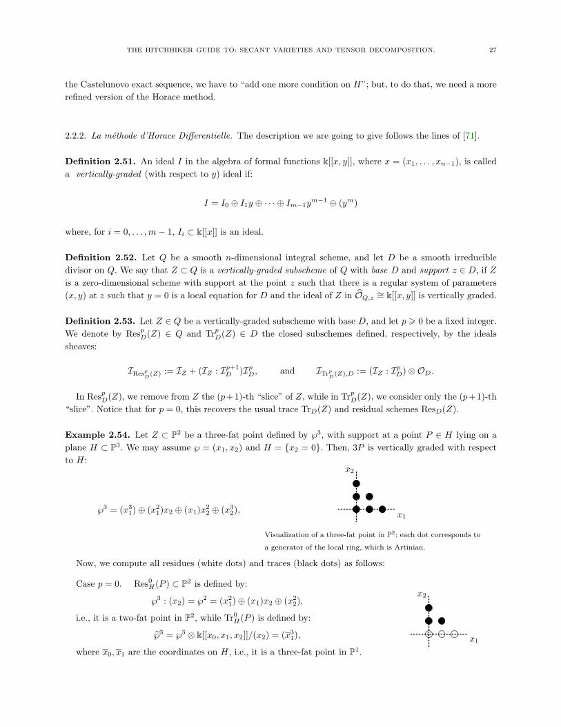
THE HITCHHIKER GUIDE TO: SECANT VARIETIES AND TENSOR DECOMPOSITION. 27
the Castelunovo exact sequence, we have to “add one more condition on H”; but, to do that, we need a morerefined version of the Horace method.
2.2.2. La methode d’Horace Differentielle. The description we are going to give follows the lines of [71].
Definition 2.51. An ideal I in the algebra of formal functions k[[x, y]], where x = (x1, . . . , xn−1), is calleda vertically-graded (with respect to y) ideal if:
I = I0 ⊕ I1y ⊕ · · · ⊕ Im−1ym−1 ⊕ (ym)
where, for i = 0, . . . ,m− 1, Ii ⊂ k[[x]] is an ideal.
Definition 2.52. Let Q be a smooth n-dimensional integral scheme, and let D be a smooth irreducibledivisor on Q. We say that Z ⊂ Q is a vertically-graded subscheme of Q with base D and support z ∈ D, if Zis a zero-dimensional scheme with support at the point z such that there is a regular system of parameters(x, y) at z such that y = 0 is a local equation for D and the ideal of Z in OQ,z ∼= k[[x, y]] is vertically graded.
Definition 2.53. Let Z ∈ Q be a vertically-graded subscheme with base D, and let p 0 be a fixed integer.We denote by RespD(Z) ∈ Q and TrpD(Z) ∈ D the closed subschemes defined, respectively, by the idealssheaves:
IRespD
(Z) := IZ + (IZ : Ip+1D )IpD, and ITrp
D(Z),D := (IZ : IpD)⊗OD.
In RespD(Z), we remove from Z the (p+1)-th “slice” of Z, while in TrpD(Z), we consider only the (p+1)-th“slice”. Notice that for p = 0, this recovers the usual trace TrD(Z) and residual schemes ResD(Z).
Example 2.54. Let Z ⊂ P2 be a three-fat point defined by ℘3, with support at a point P ∈ H lying on aplane H ⊂ P3. We may assume ℘ = (x1, x2) and H = {x2 = 0}. Then, 3P is vertically graded with respectto H:
℘3 = (x31)⊕ (x2
1)x2 ⊕ (x1)x22 ⊕ (x3
2),
x2
x1
Visualization of a three-fat point in P2: each dot corresponds to
a generator of the local ring, which is Artinian.
Now, we compute all residues (white dots) and traces (black dots) as follows:
Case p = 0. Res0H(P ) ⊂ P2 is defined by:
℘3 : (x2) = ℘2 = (x21)⊕ (x1)x2 ⊕ (x2
2),
i.e., it is a two-fat point in P2, while Tr0H(P ) is defined by:
℘3 = ℘3 ⊗ k[[x0, x1, x2]]/(x2) = (x31),
where x0, x1 are the coordinates on H, i.e., it is a three-fat point in P1.
x2
x1
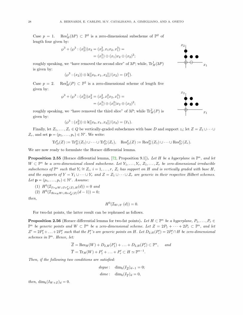
28 A. BERNARDI, E. CARLINI, M.V. CATALISANO, A. GIMIGLIANO, AND A. ONETO
Case p = 1. Res1H(3P ) ⊂ P2 is a zero-dimensional subscheme of P2 of
length four given by:
℘3 + (℘3 : (x22))x2 = (x2
2, x1x2, x31) =
= (x31)⊕ (x1)x2 ⊕ (x2)2;
roughly speaking, we “have removed the second slice” of 3P ; while, Tr1H(3P )
is given by:(℘3 : (x2))⊗ k[[x0, x1, x2]]/(x2) = (x2
1).
x2
x1
Case p = 2. Res2H(P ) ⊂ P2 is a zero-dimensional scheme of length five
given by:
℘3 + (℘3 : (x32))x2
2 = (x22, x
21x2, x
31) =
= (x31)⊕ (x2
1)x2 ⊕ (x2)2;
roughly speaking, we “have removed the third slice” of 3P ; while Tr2H(P ) is
given by:(℘3 : (x2
2))⊗ k[[x0, x1, x2]]/(x2) = (x1).
x2
x1
Finally, let Z1, . . . , Zr ∈ Q be vertically-graded subschemes with base D and support zi; let Z = Z1∪· · ·∪Zr, and set p = (p1, . . . , pr) ∈ Nr. We write:
TrpD(Z) := Trp1D (Z1) ∪ · · · ∪ TrprD (Zr), RespD(Z) := Resp1D (Z1) ∪ · · · ∪ ResprD (Zr).
We are now ready to formulate the Horace differential lemma.
Proposition 2.55 (Horace differential lemma, [72, Proposition 9.1]). Let H be a hyperplane in Pn, and letW ⊂ Pn be a zero-dimensional closed subscheme. Let Y1, . . . , Yr, Z1, . . . , Zr be zero-dimensional irreduciblesubschemes of Pn such that Yi ∼= Zi, i = 1, . . . , r, Zi has support on H and is vertically graded with base H,and the supports of Y = Y1 ∪ · · · ∪ Yr and Z = Z1 ∪ · · · ∪ Zr are generic in their respective Hilbert schemes.Let p = (p1, . . . , pr) ∈ Nr. Assume:
(1) H0(ITrHW∪TrpH(Z),H(d)) = 0 and(2) H0(IResHW∪RespH(Z)(d− 1)) = 0;
then,H0(IW∪Y (d)) = 0.
For two-fat points, the latter result can be rephrased as follows.
Proposition 2.56 (Horace differential lemma for two-fat points). Let H ⊂ Pn be a hyperplane, P1, . . . , Pr ∈Pn be generic points and W ⊂ Pn be a zero-dimensional scheme. Let Z = 2P1 + · · · + 2Pr ⊂ Pn, and letZ ′ = 2P ′1 + . . .+2P ′r such that the P ′i ’s are generic points on H. Let D2,H(P ′i ) = 2P ′i ∩H be zero-dimensionalschemes in Pn. Hence, let:
Z = ResH(W ) +D2,H(P ′1) + . . .+D2,H(P ′r) ⊂ Pn, and
T = TrH(W ) + P ′1 + . . .+ P ′r ⊂ H ' Pn−1.
Then, if the following two conditions are satisfied:
degue : dimk(IZ)d−1 = 0;
dime : dimk(IT )d = 0,
then, dimk(IW+Z)d = 0.
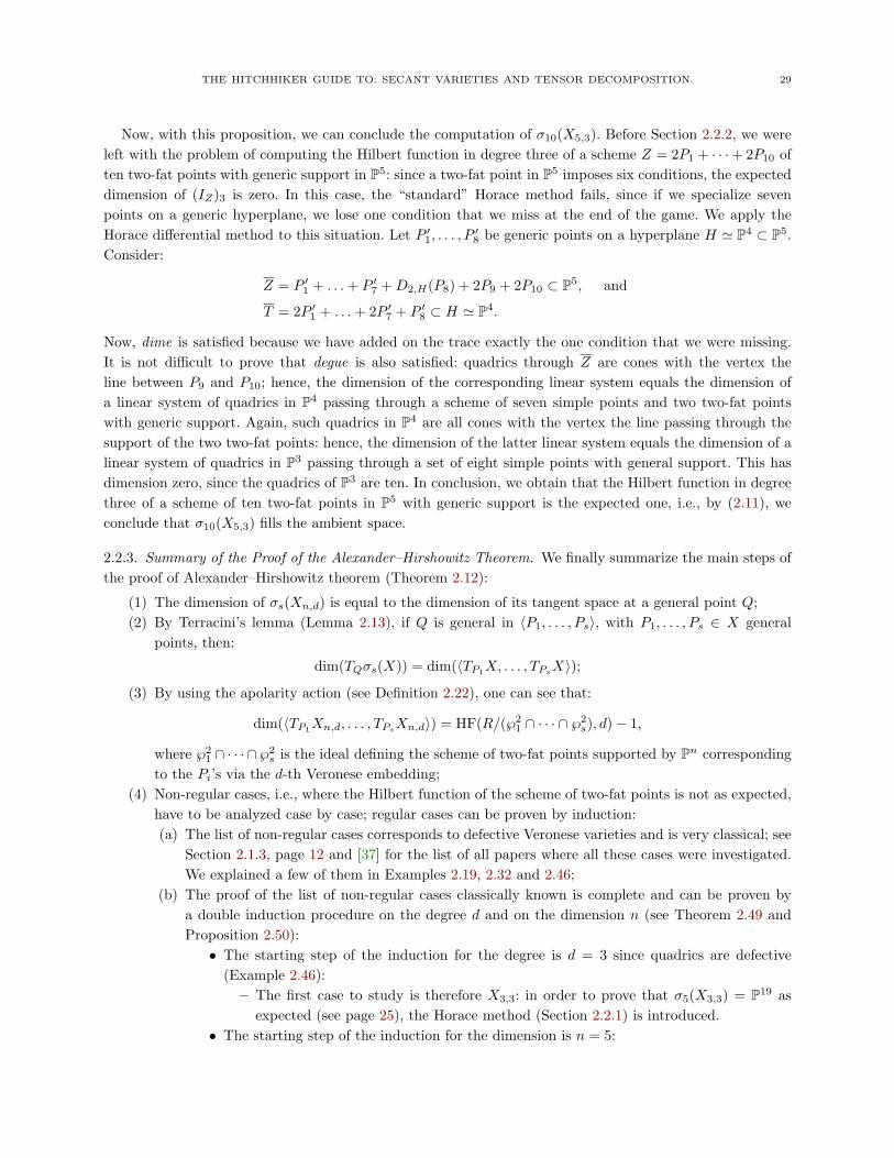
THE HITCHHIKER GUIDE TO: SECANT VARIETIES AND TENSOR DECOMPOSITION. 29
Now, with this proposition, we can conclude the computation of σ10(X5,3). Before Section 2.2.2, we wereleft with the problem of computing the Hilbert function in degree three of a scheme Z = 2P1 + · · ·+ 2P10 often two-fat points with generic support in P5: since a two-fat point in P5 imposes six conditions, the expecteddimension of (IZ)3 is zero. In this case, the “standard” Horace method fails, since if we specialize sevenpoints on a generic hyperplane, we lose one condition that we miss at the end of the game. We apply theHorace differential method to this situation. Let P ′1, . . . , P
′8 be generic points on a hyperplane H ' P4 ⊂ P5.
Consider:
Z = P ′1 + . . .+ P ′7 +D2,H(P8) + 2P9 + 2P10 ⊂ P5, and
T = 2P ′1 + . . .+ 2P ′7 + P ′8 ⊂ H ' P4.
Now, dime is satisfied because we have added on the trace exactly the one condition that we were missing.It is not difficult to prove that degue is also satisfied: quadrics through Z are cones with the vertex theline between P9 and P10; hence, the dimension of the corresponding linear system equals the dimension ofa linear system of quadrics in P4 passing through a scheme of seven simple points and two two-fat pointswith generic support. Again, such quadrics in P4 are all cones with the vertex the line passing through thesupport of the two two-fat points: hence, the dimension of the latter linear system equals the dimension of alinear system of quadrics in P3 passing through a set of eight simple points with general support. This hasdimension zero, since the quadrics of P3 are ten. In conclusion, we obtain that the Hilbert function in degreethree of a scheme of ten two-fat points in P5 with generic support is the expected one, i.e., by (2.11), weconclude that σ10(X5,3) fills the ambient space.
2.2.3. Summary of the Proof of the Alexander–Hirshowitz Theorem. We finally summarize the main steps ofthe proof of Alexander–Hirshowitz theorem (Theorem 2.12):
(1) The dimension of σs(Xn,d) is equal to the dimension of its tangent space at a general point Q;(2) By Terracini’s lemma (Lemma 2.13), if Q is general in 〈P1, . . . , Ps〉, with P1, . . . , Ps ∈ X general
points, then:
dim(TQσs(X)) = dim(〈TP1X, . . . , TPsX〉);
(3) By using the apolarity action (see Definition 2.22), one can see that:
dim(〈TP1Xn,d, . . . , TPsXn,d〉) = HF(R/(℘21 ∩ · · · ∩ ℘2
s), d)− 1,
where ℘21 ∩ · · · ∩ ℘2
s is the ideal defining the scheme of two-fat points supported by Pn correspondingto the Pi’s via the d-th Veronese embedding;
(4) Non-regular cases, i.e., where the Hilbert function of the scheme of two-fat points is not as expected,have to be analyzed case by case; regular cases can be proven by induction:(a) The list of non-regular cases corresponds to defective Veronese varieties and is very classical; see
Section 2.1.3, page 12 and [37] for the list of all papers where all these cases were investigated.We explained a few of them in Examples 2.19, 2.32 and 2.46;
(b) The proof of the list of non-regular cases classically known is complete and can be proven bya double induction procedure on the degree d and on the dimension n (see Theorem 2.49 andProposition 2.50):• The starting step of the induction for the degree is d = 3 since quadrics are defective
(Example 2.46):– The first case to study is therefore X3,3: in order to prove that σ5(X3,3) = P19 as
expected (see page 25), the Horace method (Section 2.2.1) is introduced.• The starting step of the induction for the dimension is n = 5:
30 A. BERNARDI, E. CARLINI, M.V. CATALISANO, A. GIMIGLIANO, AND A. ONETO
– σ8(X3,4) has the expected dimension thanks to upper semicontinuity (see page 26),so also the smallest secant varieties are regular (page 26);
– σ9(X3,4) is defective ([4, 44, 63]);– Therefore, one has to start with σ10(X3,5), which cannot be done with the standard
Horace method (see page 26), while it can be solved (see page 29) by using the Horacedifferential method (Section 2.2.2).
2.3. Algorithms for the Symmetric-Rank of a Given Polynomial. The goal of the second part ofthis section is to compute the symmetric-rank of a given symmetric tensor. Here, we have decided to focuson algorithms rather than entering into the details of their proofs, since most of them, especially the moreadvanced ones, are very technical and even an idea of the proofs would be too dispersive. We believe that adescriptive presentation is more enlightening on the difference among them, the punchline of each one andtheir weaknesses, rather than a precise proof.
2.3.1. On Sylvester’s Algorithm. In this section, we present the so-called Sylvester’s algorithm (Algorithm2.59). It is classically attributed to Sylvester, since he studied the problem of decomposing a homogeneouspolynomial of degree d into two variables as a sum of d-th powers of linear forms and solved it completely,obtaining that the decomposition is unique for general polynomials of odd degree. The first modern andavailable formulation of this algorithm is due to Comas and Seiguer; see [27].
Despite the “age” of this algorithm, there are modern scientific areas where it is used to describe veryadvanced tools; see [14] for the measurements of entanglement in quantum physics. The following descriptionfollows [28].
If V is a two-dimensional vector space, there is a well-known isomorphism between∧d−r+1(SdV ) and
Sd−r+1(SrV ); see [73]. In terms of projective algebraic varieties, this isomorphism allows us to view the(d − r + 1)-th Veronese embedding of Pr ' PSrV as the set of (r − 1)-dimensional linear subspaces of Pd
that are r-secant to the rational normal curve. The description of this result, via coordinates, was originallygiven by Iarrobino and Kanev; see [25]. Here, we follow the description appearing in [74] (Lemma 2.1). Weuse the notation G(k,W ) for the Grassmannian of k-dimensional linear spaces in a vector space W and thenotation G(k, n) for the Grassmannian of k-dimensional linear spaces in Pn.
Lemma 2.57. Consider the map φr,d−r+1 : P(SrV ) → G(d − r + 1, SdV ) that sends the projective class ofF ∈ SrV to the (d− r + 1)-dimensional subspace of SdV made by the multiples of F , i.e.,
φr,d−r+1([F ]) = F · Sd−rV ⊂ SdV.
Then, the following hold:
(1) the image of φr,d−r+1, after the Pl’ ucker embedding of G(d− r + 1, SdV ) inside P(∧d−r+1
SdV ), isthe (d− r + 1)-th Veronese embedding of PSrV ;
(2) identifying G(d − r + 1, SdV ) with G(r − 1,PSdV ∗), the above Veronese variety is the set of linearspaces r-secant to a rational normal curve Cd ⊂ PSdV ∗.
For the proof, we follow the constructive lines of [28], which we keep here, even though we take the proofas it is, since it is short and we believe it is constructive and useful.
THE HITCHHIKER GUIDE TO: SECANT VARIETIES AND TENSOR DECOMPOSITION. 31
Proof. Let {x0, x1} be the variables on V . Then, write F = u0xr0 + u1x
r−10 x1 + · · ·+ urx
r1 ∈ SrV . A basis of
the subspace of SdV of forms of the type FH is given by:
(2.17)
xd−r0 F = u0xd0 + · · ·+ urx
d−r0 xr1,
xd−r0 x1F = u0xd−10 x1 + · · ·+ urx
d−r−10 xr+1
1 ,...
. . .
xd−r1 F = u0xr0xd−r1 + · · ·+ urx
d1.
The coordinates of these elements with respect to the standard monomial basis {xd0, xd−10 x1, . . . , x
d1} of SdV
are thus given by the rows of the following (r + 1)× (d+ 1) matrix:
u0 u1 . . . ur 0 . . . 0 00 u0 u1 . . . ur 0 . . . 0...
. . .. . .
. . .. . .
. . ....
0 . . . 0 u0 u1 . . . ur 00 . . . 0 0 u0 . . . ur−1 ur
.
The standard Plucker coordinates of the subspace φr,d−r+1([F ]) are the maximal minors of this matrix. Itis known (see for example [29]) that these minors form a basis of k[u0, . . . , ur]d−r+1, so that the image ofφr,d−r+1([F ]) is indeed a Veronese variety, which proves (1).
To prove (2), we recall some standard facts from [29]. Consider homogeneous coordinates z0, . . . , zd inP(SdV ∗), corresponding to the dual basis of the basis {xd0, xd−1
0 x1, . . . , xd1}. Consider Cd ⊂ P(SdV ∗), the
standard rational normal curve with respect to these coordinates. Then, the image of [F ] by φr,d−r+1 isprecisely the r-secant space to Cd spanned by the divisor on Cd induced by the zeros of F . This completesthe proof of (2). �
The rational normal curve Cd ⊂ Pd is the d-th Veronese embedding of PV ' P1 inside PSdV ' Pd. Hence, asymmetric tensor F ∈ SdV has symmetric-rank r if and only if r is the minimum integer for which there existsa Pr−1 ' PW ⊂ PSdV such that F ∈ PW and PW is r-secant to the rational normal curve Cd ⊂ P(SdV ) inr distinct points. Consider the maps:
(2.18) P(SrV )φr,d−r+1−→ G(d− r,PSdV )
αr,d−r+1' G(r − 1,PSdV ∗).
Clearly, we can identify PSdV ∗ with PSdV ; hence, the Grassmannian G(r− 1,PSdV ∗) can be identified withG(r − 1,PSdV ). Now, by Lemma 2.57, a projective subspace PW of PSdV ∗ ' PSdV ' Pd is r-secant toCd ⊂ PSdV in r distinct points if and only if it belongs to Im(αr,d−r+1 ◦ φr,d−r+1) and the preimage of PWvia αr,d−r+1 ◦ φr,d−r+1 is a polynomial with r distinct roots. Therefore, a symmetric tensor F ∈ SdV hassymmetric-rank r if and only if r is the minimum integer for which the following two conditions hold:
(1) F belongs to some PW ∈ Im(αr,d−r+1 ◦ φr,d−r+1) ⊂ G(r − 1,PSdV ),(2) there exists a polynomial F ∈ SrV that has r distinct roots and such that αr,d−r+1(φr,d−r+1([F ])) =
P(W ).
Now, let PU be a (d − r)-dimensional linear subspace of PSdV . The proof of Lemma 2.57 shows that PUbelongs to the image of φr,d−r+1 if and only if there exist u0, . . . , ur ∈ k such that U = 〈F1, . . . , Fd−r+1〉,
32 A. BERNARDI, E. CARLINI, M.V. CATALISANO, A. GIMIGLIANO, AND A. ONETO
where, with respect to the standard monomial basis B = {xd0, xd−10 x1, . . . , x
d1} of SdV , we have:
F1 = (u0, u1, . . . , ur, 0, . . . , 0),
F2 = (0, u0, u1, . . . , ur, 0, . . . , 0),...
...
Fd−r+1 = (0, . . . , 0, u0, u1, . . . , ur).
Let B∗ = {z0, . . . , zd} be the dual basis of B with respect to the apolar pairing. Therefore, there exists aW ⊂ SdV such that PW = αr,d−r+1(PU) if and only if W = H1 ∩ · · · ∩Hd−r+1, and the Hi’s are as follows:
H1 : u0z0 + · · ·+ urzr = 0;
H2 : u0z1 + · · ·+ urzr+1 = 0;...
. . .
Hd−r+1 : u0zd−r + · · ·+ urzd = 0.
This is sufficient to conclude that F ∈ PSdV belongs to an (r − 1)-dimensional projective subspace ofPSdV that is in the image of αr,d−r+1 ◦ φr,d−r+1 defined in (2.18) if and only if there exist H1, . . . ,Hd−r+1
hyperplanes in SdV as above, such that F ∈ H1 ∩ . . . ∩ Hd−r+1. Now, given F ∈ SdV with coordinates(a0, . . . , ad) with respect to the dual basis B∗, we have that F ∈ H1∩ . . .∩Hd−r+1 if and only if the followinglinear system admits a non-trivial solution in the ui’s
u0a0 + · · ·+ urar = 0
u0a1 + · · ·+ urar+1 = 0. . .
u0ad−r + · · ·+ urad = 0.
If d − r + 1 < r + 1, this system admits an infinite number of solutions. If r ¬ d/2, it admits a non-trivialsolution if and only if all the maximal (r+1)-minors of the following catalecticant matrix (see Definition 2.3)vanish:
a0 · · · ara1 · · · ar+1...
...ad−r · · · ad
.
Remark 2.58. The dimension of σr(Cd) is never defective, i.e., it is the minimum between 2r − 1 and d.Actually, σr(Cd) ( PSdV if and only if 1 ¬ r <
⌈d+1
2
⌉. Moreover, an element [F ] ∈ PSdV belongs to σr(Cd)
for 1 ¬ r <⌈d+1
2
⌉, i.e., Rsym(F ) = r, if and only if Catr,d−r(F ) does not have maximal rank. These facts are
very classical; see, e.g., [1].
Therefore, if we consider the monomial basis{(
di
)−1xi0x
d−i1 | i = 0, . . . , d
}of SdV and write F =
∑di=0
(di
)−1aix
i0xd−i1 ,
then we write the (i, d− i)-th catalecticant matrix of F as Cati,d−i(F ) = (ah+k) h=0,...,ik=0,...,d−i
.
Algorithm 2.59 (Sylvester’s algorithm). The algorithm works as follows.
Input: A binary form F =∑di=0 aix
i0xd−i1 ∈ SdV .
Output: A minimal Waring decomposition F =∑ri=1 λiLi(x0, x1)d.
1: initialize r ← 0;
THE HITCHHIKER GUIDE TO: SECANT VARIETIES AND TENSOR DECOMPOSITION. 33
2: if rk Catr,d−r(F ) is maximal then3: increment r ← r + 1;4: end if5: compute a basis of Catr,d−r(F );6: take a random element G ∈ SrV ∗ in the kernel of Catr,d−r(F );7: compute the roots of G: denote them (αi, βi), for i = 1, . . . , r;8: if the roots are not distinct then9: go to Step 2;
10: else11: compute the vector λ = (λ1, . . . , λr) ∈ kr such that:
αd1 · · · αdrαd−1
1 β1 · · · αd−1r βr
αd−21 β2
1 · · · αd−2r β2
r...
......
βd1 · · · βdr
λ1
λ2...λr
=
a01da1(
d2
)−1a2
...ad
12: end if13: construct the set of linear forms {Li = αix0 + βix1} ⊂ S1V ;14: return the expression
∑ri=1 λiL
di .
Example 2.60. Compute the symmetric-rank and a minimal Waring decomposition of the polynomial
F = 2x40 − 4x3
0x1 + 30x20x
21 − 28x0x
31 + 17x4
1.
We follow Sylvester’s algorithm. The first catalecticant matrix with rank smaller than the maximal is:
Cat2,2(F ) =
2 −1 5−1 5 −75 −7 17
,
in fact, rk Cat2,2(F ) = 2. Now, let {y0, y1} the dual basis of V ∗. We get that kerCat2,2(F ) = 〈2y20−y0y1−y2
1〉.We factorize:
2y20 − y0y1 − y2
1 = (−y0 + y1)(−2y0 − y1).
Hence, we obtain the roots {(1, 1), (1,−2)}. Then, it is direct to check that:1 11 −21 41 −81 16
(
11
)=
2−15−717
,
hence, a minimal Waring decomposition is given by:
F = (x0 + x1)4 + (x0 − 2x1)4.
The following result was proven by Comas and Seiguer in [27]; see also [28]. It describes the structure ofthe stratification by symmetric-rank of symmetric tensors in SdV with dimV = 2. This result allows us toimprove the classical Sylvester algorithm (see Algorithm 2.62).
34 A. BERNARDI, E. CARLINI, M.V. CATALISANO, A. GIMIGLIANO, AND A. ONETO
Theorem 2.61. Let Cd = {[F ] ∈ PSdV | Rsym(F ) = 1} = {[Ld] | L ∈ S1V } ⊂ Pd be the rational normalcurve of degree d parametrizing decomposable symmetric tensors. Then,
∀ r, 2 ¬ r ¬⌈d+ 1
2
⌉, σr(Cd) r σr−1(Cd) = σr,r(Cd) ∪ σr,d−r+2(Cd),
where we write:σr,s(Cd) := {[F ] ∈ σr(Cd) | Rsym(F ) = s} ⊂ σr(Cd).
Algorithm 2.62 (Sylvester’s symmetric (border) rank algorithm, [28]). The latter theorem allows us to get asimplified version of the Sylvester algorithm, which computes the symmetric-rank and the symmetric-borderrank of a symmetric tensor, without computing any decomposition. Notice that Sylvester’s Algorithm 2.59for the rank is recursive: it runs for any r from one to the symmetric-rank of the given polynomial, whileTheorem 2.61 shows that once the symmetric border rank is computed, then the symmetric-rank is eitherequal to the symmetric border rank or it is d− r + 2, and this allows us to skip all the recursive process.
Input: A form F ∈ SdV , with dimV = 2.Output: the symmetric-rank Rsym(F ) and the symmetric-border rank Rsym(F ).
1: r := rk Catb d2 c,d d2 e(F )2: Rsym(F ) = r;3: choose an element G ∈ kerCatr,d−r(F );4: if G has distinct roots then5: Rsym(F ) = r
6: else7: Rsym(F ) = d− r + 2;8: end if9: return Rsym(F )
Example 2.63. Let F = 5x50x1, and let {y0, y1} be the dual basis to {x0, x1}. The smallest catalecticant
without full rank is:
Cat2,3(F ) =
0 1 0 01 0 0 00 0 0 0
,
which has rank two. Therefore [F ] ∈ σ2(C6). Now, ker Cat2,3(F ) = 〈y21〉, which has a double root. Hence,
[F ] ∈ σ2,6(C6).
Remark 2.64. When a form F ∈ k[x0, . . . , xn] can be written using less variables, i.e., F ∈ k[L0, . . . , Lm],for Lj ∈ k[x0, . . . , xn]1, with m < n, we say that F has m essential variables (in the literature, it is also saidthat F is m-concise). That is, F ∈ SdW , where W = 〈L0, . . . , Lm〉 ⊂ V . Then, the rank of [F ] with respectto Xn,d is the same one as the one with respect to νd(PW ) ⊂ Xn,d; e.g., see [75, 76]. As recently clearlydescribed in [77, Proposition 10] and more classically in [25], the number of essential variables of F coincideswith the rank of the first catalecticant matrix Cat1,d−1(F ). In particular, when [F ] ∈ σr(Xn,d) ⊂ P(SdV )with dim(V ) = n+1, then, if r < n+1, there is a subspace W ⊂ V with dim(W ) = r such that [F ] ∈ PSdW ,i.e., F can be written with respect to r variables.
Let now V be (n+ 1)-dimensional, and consider the following construction:
(2.19)
Hilbr(Pn)φ99K G
((d+nn
)− r, SdV
)
∼=
G(r − 1,PSdV ∗) ←− G((d+nn
)− r − 1,PSdV
)
THE HITCHHIKER GUIDE TO: SECANT VARIETIES AND TENSOR DECOMPOSITION. 35
where the map φ in (2.19) sends a zero-dimensional scheme Z with deg(Z) = r to the vector space (IZ)d (itis defined in the open set formed by the schemes Z, which impose independent conditions to forms of degreed) and where the last arrow is the identification, which sends a linear space to its perpendicular.
As in the case n = 1, the final image from the latter construction gives the (r − 1)-spaces, which arer-secant to the Veronese variety in PN ∼= P(k[x0, . . . , xn]d)∗. Moreover, each such space cuts the image of Zvia the Veronese embedding.
Notation 2.65. From now on, we will always use the notation ΠZ to indicate the projective linear subspaceof dimension r − 1 in PSdV , with dim(V ) = n + 1, generated by the image of a zero-dimensional schemeZ ⊂ Pn of degree r via the Veronese embedding, i.e., ΠZ = 〈νd(Z)〉 ⊂ PSdV .
Theorem 2.66. Any [F ] ∈ σ2(Xn,d) ⊂ PSdV , with dim(V ) = n+ 1 can only have symmetric-rank equal to1, 2 or d. More precisely:
σ2(Xn,d) rXn,d = σ2,2(Xn,d) ∪ σ2,d(Xn,d);
more precisely, σ2,d(Xn,d) = τ(Xn,d) rXn,d, where τ(Xn,d) denotes the tangential variety of Xn,d, i.e., theZariski closure of the union of the tangent spaces to Xn,d.
Proof. This is actually a quite direct consequence of Remark 2.64 and of Theorem 2.61, but let us describethe geometry in some detail, following the proof of [28]. Since r = 2, every Z ∈ Hilb2(Pn) is the completeintersection of a line and a quadric, so the structure of IZ is well known, i.e., IZ = (L0, . . . , Ln−2, Q), whereLi’s are linearly independent linear forms and Q is a quadric in S2V r (L0, . . . , Ln−2)2.
If F ∈ σ2(Xn,d), then we have two possibilities: either Rsym(F ) = 2 or Rsym(T ) > 2, i.e., F lies on atangent line ΠZ to the Veronese, which is given by the image of a scheme Z ⊂ PV of degree 2, via the maps(2.19). We can view F in the projective linear space H ∼= Pd in P(SdV ) generated by the rational normalcurve Cd ⊂ Xn,d, which is the image of the line ` defined by the ideal (L0, . . . , Ln−2) in PV , i.e., ` ⊂ Pn is theunique line containing Z. Hence, we can apply Theorem 2.61 in order to get that Rsym(F ) ¬ d. Moreover,by Remark 2.64, we have Rsym(F ) = d. �
Remark 2.67. Let us check that σ2(Xn,d) is given by the annihilation of the (3 × 3)-minors of the firsttwo catalecticant matrices, Cat1,d−1(V ) and Cat2,d−2(V ) (see Definition 2.3); actually, such minors are thegenerators of Iσ2(νd(Pn)); see [78].
Following the construction above (2.19), we can notice that the coefficients of the linear spaces defined bythe forms Li ∈ V ∗ in the ideal IZ are the solutions of a linear system whose matrix is given by the catalecticantmatrix Cat1,d−1(V ); since the space of solutions has dimension n− 1, we get rk Cat1,d−1(V ) = 2. When weconsider the quadric Q in IZ , instead, the analogous construction gives that its coefficients are the solutionsof a linear system defined by the catalecticant matrix Cat2,d−2(V ), and the space of solutions give Q and allthe quadrics in (L0, . . . , Ln−2)2, which are
(n2
)+ 2n− 1, hence:
rk Cat2,d−2(V ) =(n+ 2
2
)−((
n
2
)+ 2n
)= 2.
Therefore, we can write down an algorithm (Algorithm 2.68) to test if an element [F ] ∈ σ2(Xn,d) hassymmetric rank two or d.
Algorithm 2.68 (An algorithm to compute the symmetric-rank of an element lying on σ2(Xn,d)). Input:A from F ∈ SdV , where dimV = n+ 1.
Output: If [F ] ∈ σ2(Xn,d), returns the Rsym(F ).1: compute the number of essential variables m = rk Cat1,d−1(F );2: if m = 1 then
36 A. BERNARDI, E. CARLINI, M.V. CATALISANO, A. GIMIGLIANO, AND A. ONETO
3: print F ∈ Xn,d;4: else if m > 2 then5: print F 6∈ σ2(Xn,d);6: else7: let W = (kerCat1,d−1(F ))⊥ and view F ∈ SdW ;8: end if9: return apply Algorithm 2.62 to F .
Example 2.69. Compute the symmetric-rank of
F = x30x2 + 3x2
0x1x2 + 3x0x21x2 + x3
1x2.
First of all, note that (y0 − y1) ◦ F = 0; in particular, kerCat1,3(F ) = 〈y0 − y1〉. Hence, F has two essentialvariables. This can also be seen by noticing that F = (x0 + x1)3x2. Therefore, if we write z0 = x0 + x1
and z1 = x2, then F = z30z1 ∈ k[z0, z1]. Hence, we can apply Algorithm 2.59 and 2.62 to compute the
symmetric-rank, symmetric-border rank and a minimal decompositions of F . In particular, we write:
Cat2,2(F ) =
0 1/4 01/4 0 00 0 0
,
which has rank two, as expected. Again, as in Example 2.63, the kernel of Cat2,2(F ) defines a polynomial witha double root. Hence, Rsym(F ) = 2 and Rsym(F ) = 4. If we are interested in finding a minimal decompositionof F , we have to consider the first catalecticant whose kernel defines a polynomial with simple roots. In thiscase, we should get to:
Cat0,4(F ) =
0
1/4000
,
whose kernel is 〈(1, 0, 0, 0, 0), (0, 0, 1, 0, 0), (0, 0, 0, 1, 0), (0, 0, 0, 0, 1)〉. If we let {w0, w1} be the variables onW ∗, we take a polynomial in this kernel, as for example G = w4
0 + w20w
21 + w0w
31 + w4
1. Now, if we computethe roots of G, we find four complex distinct roots, i.e.,
(α1, β1) = − 16A−
12
√B + C (α2, β2) = − 1
6A+ 12
√B + C;
(α3, β3) = 16A−
12
√B − C (α4, β4) = 1
6A+ 12
√B − C;
where:
A =
√√√√9 ( 118 i√257√3− 4354) 23 − 6 ( 118 i√257√3− 4354) 13 + 13118 i√257√3− 4354
13
;
B =
√−(1/18i
√257√3− 4354
)1/3−( 13
9118 i√257√3− 4354
) 13
;
C =6√
9( 118 i√257√3− 4354 )
23−6( 118 i
√257√3− 4354 )
13 +13
118 i√257√(3)− 4354
13
− 43
THE HITCHHIKER GUIDE TO: SECANT VARIETIES AND TENSOR DECOMPOSITION. 37
Hence, if we write Li = αiz0 + βiz1, for i = 1, . . . , 4, we can find suitable λi’s to write a minimal de-composition F =
∑4i=1 λiL
4i . Observe that any hyperplane through [F ] that does not contain the tan-
gent line to C4 at [z40 ] intersects C4 at four distinct points, so we could have chosen also another point in
〈(1, 0, 0, 0, 0), (0, 0, 1, 0, 0), (0, 0, 0, 1, 0), (0, 0, 0, 0, 1)〉, and we would have found another decomposition of F .
Everything that we have done in this section does not use anything more than Sylvester’s algorithm forthe two-variable case. In the next sections, we see what can be done if we have to deal with more variablesand we cannot reduce to the binary case like in Example 2.69.
Sylvester’s algorithm allows us to compute the symmetric-rank of any polynomial in two essential variables.It is mainly based on the fact that equations for secant varieties of rational normal curves are well known andthat there are only two possibilities for the symmetric-rank of a given binary polynomial with fixed borderrank (Theorem 2.61). Moreover, those two cases are easily recognizable by looking at the multiplicity of theroots of a generic polynomial in the kernel of the catalecticant.
The first ideas that were exploited to generalize Sylvester’s result to homogeneous polynomials in morethan two variables were:
• a good understanding of the inverse system (and therefore, of the scheme defined by the kernels ofcatalecticant matrices and possible extension of catalecticant matrices, namely Hankel matrices); wewill go into the details of this idea in Section 2.3.3;
• a possible classification of the ranks of polynomials with fixed border rank; we will show the fewresults in this direction in Section 2.3.2.
2.3.2. Beyond Sylvester’s Algorithm Using Zero-Dimensional Schemes. We keep following [28]. Let us startby considering the case of a homogeneous polynomial with three essential variables.
If [F ] ∈ σ3(νd(Pn))rσ2(νd(Pn)), then we will need more than two variables, but actually, three are alwayssufficient. In fact, if [F ] ∈ σ3(νd(Pn)), then there always exists a zero-dimensional scheme νd(Z) of lengththree contained in νd(Pn), whose span contains [F ]; the scheme Z ⊂ Pn itself spans a P2, which can be seen asP((L1, L2, L3)1) with Li’s linear forms. Therefore, F can be written in three variables. The following theoremcomputes the symmetric-rank of any polynomial in [F ] ∈ σ3(νd(Pn)) \ σ2(νd(Pn)), and the idea is to classifythe symmetric-rank by looking at the structure of the zero-dimensional scheme of length three, whose linearspan contains [F ].
Theorem 2.70 ([28, Theorem 37]). Let d 3, Xn,d ⊂ P(kn+1). Then,
σ3(Xn,3) r σ2(Xn,3) = σ3,3(Xn,3) ∪ σ3,4(Xn,3) ∪ σ3,5(Xn,3),
while, for d 4,
σ3(Xn,d) r σ2(Xn,d) = σ3,3(Xn,d) ∪ σ3,d−1(Xn,d) ∪ σ3,d+1(Xn,d) ∪ σ3,2d−1(Xn,d).
We do not give here all the details of the proof since they can be found in [28]; they are quite technical,but the main idea is the one described above. We like to stress that the relation between the zero-dimensionalscheme of length three spanning F and the one computing the symmetric-rank is in many cases dependent onthe following Lemma 2.71. Probably, it is classically known, but we were not able to find a precise reference.
Lemma 2.71 ([28] (Lemma 11)). Let Z ⊂ Pn, n 2, be a zero-dimensional scheme, with deg(Z) ¬ 2d+ 1.A necessary and sufficient condition for Z to impose independent conditions on hypersurfaces of degree d isthat no line ` ⊂ Pn is such that deg(Z ∩ `) d+ 2.
Remark 2.72. Notice that if deg(` ∩ Z) is exactly d + 1 + k, then the dimension of the space of curves ofdegree d through them is increased exactly by k with respect to the generic case.
38 A. BERNARDI, E. CARLINI, M.V. CATALISANO, A. GIMIGLIANO, AND A. ONETO
It is easy to see that Lemma 2.71 can be improved as follows; see [79].
Lemma 2.73 ([79]). Let Z ⊂ Pn, n 2, be a zero-dimensional scheme, with deg(Z) ¬ 2d + 1. Ifh1(Pn, IZ(d)) > 0, there exists a unique line ` ⊂ Pn such that deg(Z ∩ `) = d+ 1 + h1(Pn, IZ(d)) > 0.
We can go back to our problem of finding the symmetric-rank of a given tensor. The classification ofsymmetric-ranks of the elements in σ4(Xn,d) can be treated in an analogous way as we did for σ3(Xn,d), butunfortunately, it requires a very complicated analysis on the schemes of length four. This is done in [80], butbecause of the long procedure, we prefer to not present it here.
It is remarkable that σ4(Xn,d) is the last s-th secant variety of Veronesean, where we can use this techniquefor the classification of the symmetric-rank with respect to zero-dimensional schemes of length s, whose spancontains the given polynomial we are dealing with; for s 5, there is a more intrinsic problem. In fact, thereis a famous counterexample due to Buczyńska and Buczyśki (see [81]) that shows that, in σ5(X4,3), thereis at least a polynomial for which there does not exist any zero-dimensional scheme of length five on X4,3,whose span contains it. The example is the following.
Example 2.74 (Buczyńska, Buczyński [81, 82]). One can easily check that the following polynomial:
F = x20x2 + 6x2
1x3 − 3 (x0 + x1)2x4.
can be obtained as limε→013εFε = F where:
Fε = (x0 + εx2)3 + 6(x1 + εx3)3 − 3(x0 + x1 + εx4)3 + 3(x0 + 2x1)3 − (x0 + 3x1)3
has symmetric-rank five for ε > 0. Therefore, [F ] ∈ σ5(ν3(P4)).An explicit computation of F⊥ yields the Hilbert series for HSR/F⊥(z) = 1 + 5z + 5z2 + z3. Let us prove,
by contradiction, that there is no saturated ideal I ⊂ F⊥ defining a zero-dimensional scheme of length ¬ 5.Suppose on the contrary that I is such an ideal. Then, HFR/I(i) HFR/F⊥(i) for all i ∈ N. As HFR/I(i) isan increasing function of i ∈ N with HFR/F⊥(i) ¬ HFR/I(i) ¬ 5, we deduce that HSR/I(t) = 1 + 5
∑∞i=1 z
i.This shows that I1 = {0} and that I2 = (F⊥)2. As I is saturated, I2 : (x0, . . . , x4) = I1 = {0}, sinceHFR/F⊥(1) = 5. However, an explicit computation of (F⊥)2 : (x0, . . . , x4) gives 〈x2, x3, x4〉. In this way, weobtain a contradiction, so that there is no saturated ideal of degree ¬ 5 such that I ⊂ F⊥. Consequently, theminimal zero-dimensional scheme contained in X4,3 whose linear span contains [F ] has degree six.
In the best of our knowledge, the two main results that are nowadays available to treat these “wild” casesare the following.
Proposition 2.75 ([28]). Let X ⊂ PN be a non-degenerate smooth variety. Let Hr be the irreducible com-ponent of the Hilbert scheme of zero-dimensional schemes of degree r of X containing r distinct points, andassume that for each y ∈ Hr, the corresponding subscheme Y of X imposes independent conditions on linearforms. Then, for each P ∈ σr(X) rσ0
r(X), there exists a zero-dimensional scheme Z ⊂ X of degree r suchthat P ∈ 〈Z〉 ∼= Pr−1. Conversely, if there exists Z ∈ Hr such that P ∈ 〈Z〉, then P ∈ σr(X).
Obviously, five points on a line do not impose independent conditions on cubics in any Pn for n 5;therefore, this could be one reason why the counterexample given in Example 2.74 is possible. Anotherreason is the following.
Proposition 2.76 ([81]). Suppose there exist points P1, . . . , Pr ∈ X that are linearly degenerate, that isdim〈P1, . . . , Pr〉 < r−1. Then, the join of the r tangent stars (see [83] (Section 1.4) for a definition) at thesepoints is contained in σr(X). In the case that X is smooth at P1, . . . Pr, then 〈TP1X, . . . , TPrX〉 ⊂ σr(X).
THE HITCHHIKER GUIDE TO: SECANT VARIETIES AND TENSOR DECOMPOSITION. 39
2.3.3. Beyond Sylvester’s Algorithm via Apolarity. We have already defined in Section 2.1.4 the apolarityaction of S•V ∗ ' k[y0, . . . , yn] on S•V ' k[x0, . . . , xn] and inverse systems. Now, we introduce the mainalgebraic tool from apolarity theory to study ranks and minimal Waring decompositions: that is the apolaritylemma; see [25, 24]. First, we introduce the apolar ideal of a polynomial.
Definition 2.77. Let F ∈ SdV be a homogeneous polynomial. Then, the apolar ideal of F is:
F⊥ = {G ∈ S•V ∗ | G ◦ F = 0}.
Remark 2.78. The apolar ideal is a homogeneous ideal. Clearly, F⊥i = SiV ∗, for any i > d, namelyAF = S•V ∗/F⊥ is an Artinian algebra with socle degree equal to d. Since dimk(AF )d = 1, then it is also aGorenstein algebra. Actually, Macaulay proved that there exists a one-to-one correspondence between gradedArtinian Gorenstein algebras with socle degree d and homogeneous polynomials of degree d; for details, see[24, Theorem 8.7].
Remark 2.79. Note that, directly by the definitions, the non-zero homogeneous parts of the apolar ideal ofa homogeneous polynomial F coincide with the kernel of its catalecticant matrices, i.e., for i = 0, . . . , d,
F⊥i = ker(Cati,d−i(F )).
The apolarity lemma tells us that Waring decompositions of a given polynomial correspond to sets ofreduced points whose defining ideal is contained in the apolar ideal of the polynomial.
Lemma 2.80 (Apolarity lemma). Let Z = {[L1], . . . , [Lr]} ⊂ P(S1V ), then the following are equivalent:
(1) F =∑ri=1 λiL
di , for some λ1, . . . , λr ∈ k;
(2) I(Z) ⊆ F⊥.
If these conditions hold, we say that Z is a set of points apolar to F .
Proof. The fact that (1) implies (2) follows from the easy fact that, for any G ∈ SdV ∗, we have that G ◦ Ld
is equal to d times the evaluation of G at the point [L] ∈ PV . Conversely, if I(Z) ⊂ F⊥, then we have thatF ∈ I(Z)⊥d = 〈Ld1, . . . , Ldr〉; see Remark 2.28 and Proposition 2.29. �
Remark 2.81 (Yet again: Sylvester’s algorithm). With this lemma, we can rephrase Sylvester’s algorithm.Consider the binary form F =
∑di=0 ci
(di
)xd−i0 xi1. Such an F can be decomposed as the sum of r distinct
powers of linear forms if and only if there exists Q = q0yr0 + q1y
r−10 y1 + · · ·+ qry
r1 such that:
(2.20)
c0 c1 · · · crc1 · · · cr+1...
...cd−r · · · cd
q0
q1...qr
= 0,
and Q = µΠrk=1(βky0 − αky1), for a suitable scalar µ ∈ k, where [αi : βi]’s are different points in P1. In this
case, there exists a choice of λ1, . . . , λr such that F =∑rk=1 λk(αkx0 + βkx1)d. This is possible because of
the following remarks:
• Gorenstein algebras of codimension two are always complete intersections, i.e.,
I(Z) ⊂ (F⊥) = (G1, G2);
• Artinian Gorenstein rings have a symmetric Hilbert function, hence:
deg(G1) + deg(G2) = deg(F ) + 2, say deg(G1) ¬ deg(G2);
40 A. BERNARDI, E. CARLINI, M.V. CATALISANO, A. GIMIGLIANO, AND A. ONETO
• If G1 is square-free, i.e., has only distinct roots, we take Q = G1 and Rsym(F ) = deg(G1); otherwise,the first degree where we get something square-free has to be the degree of G2; in particular, we cantake Q to be a generic element in F⊥deg(G2)
and Rsym(F ) = deg(G2).
By using Apolarity Theory, we can describe the following algorithm (Algorithm 2.82).
Algorithm 2.82 (Iarrobino and Kanev, [25].). We attribute the following generalization of Sylvester’s al-gorithm to any number of variables to Iarrobino and Kanev: despite that they do not explicitly write thealgorithm, the main idea is presented in [25]. Sometimes, this algorithm is referred to as the catalecticantmethod.
Input: F ∈ SdV , where dimV = n+ 1.Output: a minimal Waring decomposition.
1: construct the most square catalecticant of F , i.e., Catm,d−m(F ) for m = dd/2e;2: compute kerCatm,d−m(F );3: if the zero-set Z of the polynomials in kerCatm,d−m(F ) is a reduced set of points, say {[L1], . . . , [Lr]},
then continue, otherwise the algorithm fails;4: solve the linear system defined by F =
∑si=1 λiL
di in the unknowns λi.
Example 2.83. Compute a Waring decomposition of:
F = 3x4 + 12x2y2 + 2y4 − 12x2yz + 12xy2z − 4y3z + 12x2z2 − 12xyz2 + 6y2z2 − 4yz3 + 2z4.
The most square catalecticant matrix is:
Cat2,2(F ) =
3 0 0 2 −1 20 2 −1 0 1 −10 −1 2 1 −1 02 0 1 2 −1 1−1 1 −1 −1 1 −1
2 −1 0 1 −1 2
.
Now, compute that the rank of Cat2,2(F ) is three, and its kernel is:
ker(Cat2,2(F )) = 〈(1, 0, 0,−1,−1,−1), (0, 1, 0,−1,−2, 0), (0, 0, 1, 0, 2, 1)〉 =
〈y20 − y2
1 − y1y2 − y22 , y0y1 − y2
1 − 2y1y2, y0y2 + 2y1y2 + y22〉 ⊂ S2V ∗.
It is not difficult to see that these three quadrics define a set of reduced points {[1 : 1 : 0], [1 : 0 : −1], [1 :−1 : 1]} ⊂ PV . Hence, we take L1 = x0 + x1, L2 = x0 − x2 and L3 = x0 − x1 + x2, and, by the apolaritylemma, the polynomial F is a linear combinations of those forms, in particular,
F = (x0 + x1)4 + (x0 − x2)4 + (x0 − x1 + x2)4.
Clearly, this method works only if Rsym(F ) = rank Catm,d−m(F ), for m =⌈d2
⌉. Unfortunately, in many
cases, this condition is not always satisfied.Algorithm 2.82 has been for a long time the only available method to handle the computation of the
decomposition of polynomials with more than two variables. In 2013, there was an interesting contributiondue to Oeding and Ottaviani (see [84]), where the authors used vector bundle techniques introduced in [85]to find non-classical equations of certain secant varieties. In particular, the very interesting part of the paper[84] is the use of representation theory, which sheds light on the geometric aspects of this algorithm andrelates these techniques to more classical results like the Sylvester pentahedral theorem (the decompositionof cubic polynomial in three variables as the sum of five cubes). For the heaviness of the representation theory
THE HITCHHIKER GUIDE TO: SECANT VARIETIES AND TENSOR DECOMPOSITION. 41
background needed to understand that algorithm, we have chosen to not present it here. Moreover, we have topoint out that [84] (Algorithm 4) fails whenever the symmetric-rank of the polynomial is too large comparedto the rank of a certain matrix constructed with the techniques introduced in [84], similarly as happens forthe catalecticant method.
Nowadays, one of the best ideas to generalize the method of catalecticant matrices is due to Brachat,Comon, Mourrain and Tsidgaridas, who in [30] developed an algorithm (Algorithm 2.92) that gets rid of therestrictions imposed by the usage of catalecticant matrices. The idea developed in [30] is to use the so-calledHankel matrix that in a way encodes all the information of all the catalecticant matrices. The algorithmpresented in [30] to compute a Waring decomposition of a form F ∈ SdV passes through the computationof an affine Waring decomposition of the dehomogenization f of the given form with respect to a suitablevariable. Let S = k[x1, . . . , xn] be the polynomial ring in n variables over the field k corresponding to suchdehomogenization.
We first need to introduce the definition of Hankel operator associated with any Λ ∈ S∗. To do so, weneed to use the structure of S∗ as the S-module, given by:
a ∗ Λ : S → k, b 7→ Λ(ab), for a ∈ S,Λ ∈ S∗.
Then, the Hankel operator associated with Λ ∈ S∗ is the matrix associated with the linear map:
HΛ : S → S∗, such that a 7→ a ∗ Λ.
Here are some useful facts about Hankel operators.
Proposition 2.84. ker(HΛ) is an ideal.
Let IΛ = ker(HΛ) and AΓ = S/IΛ.
Proposition 2.85. If rank(HΛ) = r <∞, then the algebra AΛ is a k-vector space of dimension r, and thereexist polynomials l1, . . . lk of degree one and g1, . . . , gk of degree d1, . . . , dk, respectively, in k[∂1, . . . , ∂n] suchthat:
Λ =k∑i=1
ld−dii gi.
Moreover, IΛ defines the union of affine schemes Z1, . . . , Zk with support on the points l∗1, . . . , l∗k ∈ kn,
respectively, and with multiplicity equal to the dimension of the vector space spanned by the inverse systemgenerated by ld−dii gi.
The original proof of this proposition can be found in [30]; for a more detailed and expanded presentation,see [32, 31].
Theorem 2.86 (Brachat, Comon, Mourrain, Tsigaridas [30]). An element Λ ∈ S∗ can be decomposed asΛ =
∑ri=1 λil
di if and only if rankHΛ = r, and IΛ is a radical ideal.
Now, we consider the multiplication operators in AΛ. Given a ∈ AΛ:
Ma : AΛ → AΛ,
b 7→ a · b,and,
M ta : A∗Λ → A∗Λ,
γ 7→ a ∗ γ.Now,
(2.21) Ha∗Λ := M ta ·HΛ.
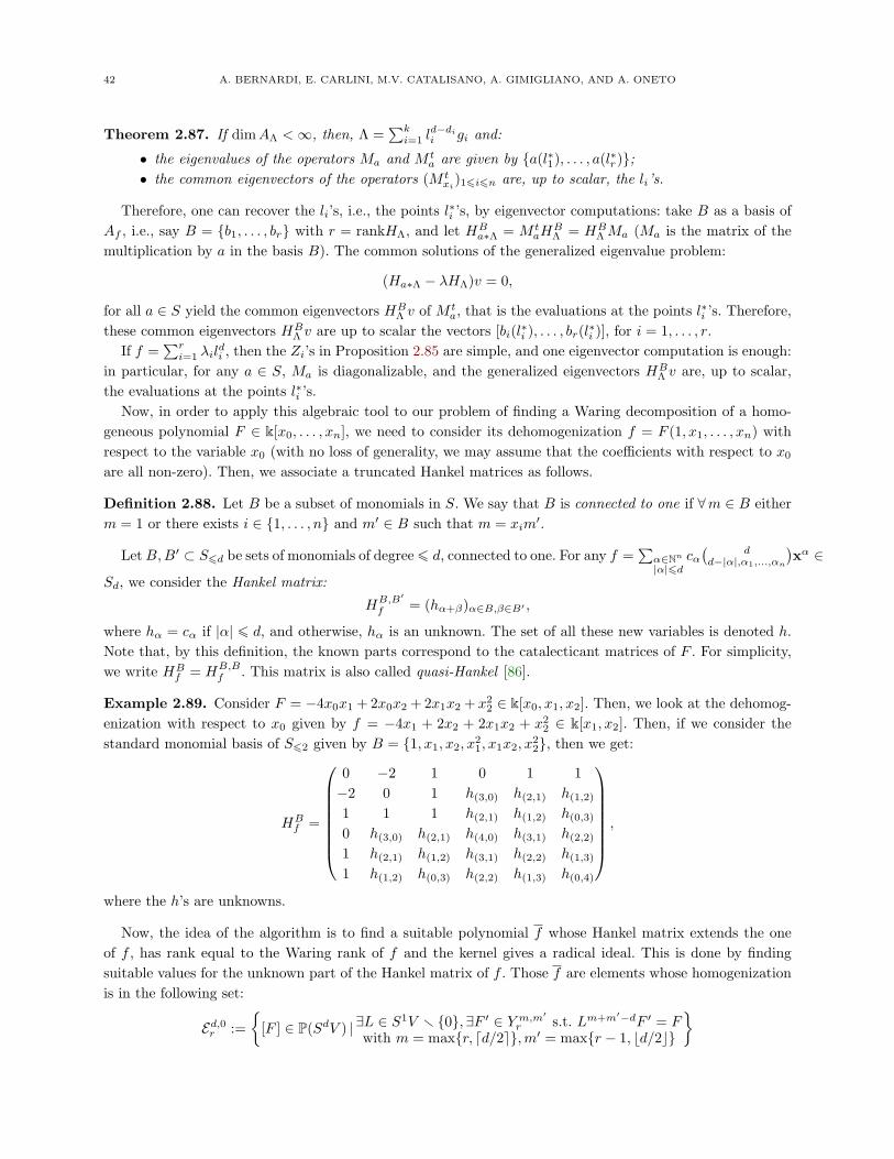
42 A. BERNARDI, E. CARLINI, M.V. CATALISANO, A. GIMIGLIANO, AND A. ONETO
Theorem 2.87. If dimAΛ <∞, then, Λ =∑ki=1 l
d−dii gi and:
• the eigenvalues of the operators Ma and M ta are given by {a(l∗1), . . . , a(l∗r)};
• the common eigenvectors of the operators (M txi)1¬i¬n are, up to scalar, the li’s.
Therefore, one can recover the li’s, i.e., the points l∗i ’s, by eigenvector computations: take B as a basis ofAf , i.e., say B = {b1, . . . , br} with r = rankHΛ, and let HB
a∗Λ = M taH
BΛ = HB
Λ Ma (Ma is the matrix of themultiplication by a in the basis B). The common solutions of the generalized eigenvalue problem:
(Ha∗Λ − λHΛ)v = 0,
for all a ∈ S yield the common eigenvectors HBΛ v of M t
a, that is the evaluations at the points l∗i ’s. Therefore,these common eigenvectors HB
Λ v are up to scalar the vectors [bi(l∗i ), . . . , br(l∗i )], for i = 1, . . . , r.
If f =∑ri=1 λil
di , then the Zi’s in Proposition 2.85 are simple, and one eigenvector computation is enough:
in particular, for any a ∈ S, Ma is diagonalizable, and the generalized eigenvectors HBΛ v are, up to scalar,
the evaluations at the points l∗i ’s.Now, in order to apply this algebraic tool to our problem of finding a Waring decomposition of a homo-
geneous polynomial F ∈ k[x0, . . . , xn], we need to consider its dehomogenization f = F (1, x1, . . . , xn) withrespect to the variable x0 (with no loss of generality, we may assume that the coefficients with respect to x0
are all non-zero). Then, we associate a truncated Hankel matrices as follows.
Definition 2.88. Let B be a subset of monomials in S. We say that B is connected to one if ∀m ∈ B eitherm = 1 or there exists i ∈ {1, . . . , n} and m′ ∈ B such that m = xim
′.
LetB,B′ ⊂ S¬d be sets of monomials of degree¬ d, connected to one. For any f =∑α∈Nn|α|¬d
cα(
dd−|α|,α1,...,αn
)xα ∈
Sd, we consider the Hankel matrix:
HB,B′
f = (hα+β)α∈B,β∈B′ ,
where hα = cα if |α| ¬ d, and otherwise, hα is an unknown. The set of all these new variables is denoted h.Note that, by this definition, the known parts correspond to the catalecticant matrices of F . For simplicity,we write HB
f = HB,Bf . This matrix is also called quasi-Hankel [86].
Example 2.89. Consider F = −4x0x1 + 2x0x2 + 2x1x2 + x22 ∈ k[x0, x1, x2]. Then, we look at the dehomog-
enization with respect to x0 given by f = −4x1 + 2x2 + 2x1x2 + x22 ∈ k[x1, x2]. Then, if we consider the
standard monomial basis of S¬2 given by B = {1, x1, x2, x21, x1x2, x
22}, then we get:
HBf =
0 −2 1 0 1 1−2 0 1 h(3,0) h(2,1) h(1,2)
1 1 1 h(2,1) h(1,2) h(0,3)
0 h(3,0) h(2,1) h(4,0) h(3,1) h(2,2)
1 h(2,1) h(1,2) h(3,1) h(2,2) h(1,3)
1 h(1,2) h(0,3) h(2,2) h(1,3) h(0,4)
,
where the h’s are unknowns.
Now, the idea of the algorithm is to find a suitable polynomial f whose Hankel matrix extends the oneof f , has rank equal to the Waring rank of f and the kernel gives a radical ideal. This is done by findingsuitable values for the unknown part of the Hankel matrix of f . Those f are elements whose homogenizationis in the following set:
Ed,0r :={
[F ] ∈ P(SdV ) | ∃L ∈ S1V r {0},∃F ′ ∈ Y m,m′r s.t. Lm+m′−dF ′ = F
with m = max{r, dd/2e},m′ = max{r − 1, bd/2c}
}
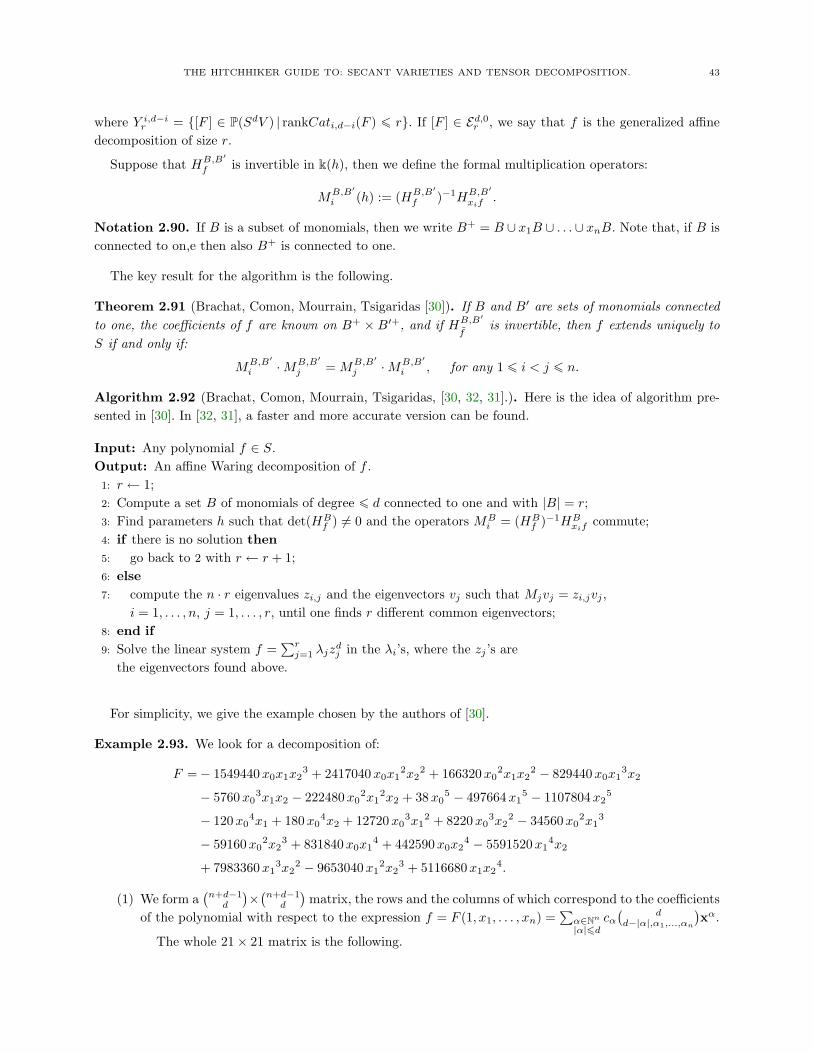
THE HITCHHIKER GUIDE TO: SECANT VARIETIES AND TENSOR DECOMPOSITION. 43
where Y i,d−ir = {[F ] ∈ P(SdV ) | rankCati,d−i(F ) ¬ r}. If [F ] ∈ Ed,0r , we say that f is the generalized affinedecomposition of size r.
Suppose that HB,B′
f is invertible in k(h), then we define the formal multiplication operators:
MB,B′
i (h) := (HB,B′
f )−1HB,B′
xif.
Notation 2.90. If B is a subset of monomials, then we write B+ = B ∪ x1B ∪ . . .∪ xnB. Note that, if B isconnected to on,e then also B+ is connected to one.
The key result for the algorithm is the following.
Theorem 2.91 (Brachat, Comon, Mourrain, Tsigaridas [30]). If B and B′ are sets of monomials connectedto one, the coefficients of f are known on B+ × B′+, and if HB,B′
fis invertible, then f extends uniquely to
S if and only if:
MB,B′
i ·MB,B′
j = MB,B′
j ·MB,B′
i , for any 1 ¬ i < j ¬ n.
Algorithm 2.92 (Brachat, Comon, Mourrain, Tsigaridas, [30, 32, 31].). Here is the idea of algorithm pre-sented in [30]. In [32, 31], a faster and more accurate version can be found.
Input: Any polynomial f ∈ S.Output: An affine Waring decomposition of f .
1: r ← 1;2: Compute a set B of monomials of degree ¬ d connected to one and with |B| = r;3: Find parameters h such that det(HB
f ) 6= 0 and the operators MBi = (HB
f )−1HBxif
commute;4: if there is no solution then5: go back to 2 with r ← r + 1;6: else7: compute the n · r eigenvalues zi,j and the eigenvectors vj such that Mjvj = zi,jvj ,
i = 1, . . . , n, j = 1, . . . , r, until one finds r different common eigenvectors;8: end if9: Solve the linear system f =
∑rj=1 λjz
dj in the λi’s, where the zj ’s are
the eigenvectors found above.
For simplicity, we give the example chosen by the authors of [30].
Example 2.93. We look for a decomposition of:
F =− 1549440x0x1x23 + 2417040x0x1
2x22 + 166320x0
2x1x22 − 829440x0x1
3x2
− 5760x03x1x2 − 222480x0
2x12x2 + 38x0
5 − 497664x15 − 1107804x2
5
− 120x04x1 + 180x0
4x2 + 12720x03x1
2 + 8220x03x2
2 − 34560x02x1
3
− 59160x02x2
3 + 831840x0x14 + 442590x0x2
4 − 5591520x14x2
+ 7983360x13x2
2 − 9653040x12x2
3 + 5116680x1x24.
(1) We form a(n+d−1
d
)×(n+d−1
d
)matrix, the rows and the columns of which correspond to the coefficients
of the polynomial with respect to the expression f = F (1, x1, . . . , xn) =∑α∈Nn|α|¬d
cα(
dd−|α|,α1,...,αn
)xα.
The whole 21× 21 matrix is the following.
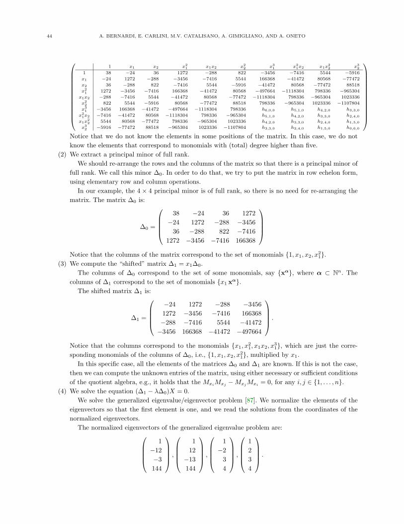
44 A. BERNARDI, E. CARLINI, M.V. CATALISANO, A. GIMIGLIANO, AND A. ONETO
1 x1 x2 x21 x1x2 x22 x31 x21x2 x1x22 x32
1 38 −24 36 1272 −288 822 −3456 −7416 5544 −5916x1 −24 1272 −288 −3456 −7416 5544 166368 −41472 80568 −77472x2 36 −288 822 −7416 5544 −5916 −41472 80568 −77472 88518x21 1272 −3456 −7416 166368 −41472 80568 −497664 −1118304 798336 −965304x1x2 −288 −7416 5544 −41472 80568 −77472 −1118304 798336 −965304 1023336x22 822 5544 −5916 80568 −77472 88518 798336 −965304 1023336 −1107804x31 −3456 166368 −41472 −497664 −1118304 798336 h6,0,0 h5,1,0 h4,2,0 h3,3,0x21x2 −7416 −41472 80568 −1118304 798336 −965304 h5,1,0 h4,2,0 h3,3,0 h2,4,0x1x
22 5544 80568 −77472 798336 −965304 1023336 h4,2,0 h3,3,0 h2,4,0 h1,5,0
x32 −5916 −77472 88518 −965304 1023336 −1107804 h3,3,0 h2,4,0 h1,5,0 h0,6,0
Notice that we do not know the elements in some positions of the matrix. In this case, we do notknow the elements that correspond to monomials with (total) degree higher than five.
(2) We extract a principal minor of full rank.We should re-arrange the rows and the columns of the matrix so that there is a principal minor of
full rank. We call this minor ∆0. In order to do that, we try to put the matrix in row echelon form,using elementary row and column operations.
In our example, the 4 × 4 principal minor is of full rank, so there is no need for re-arranging thematrix. The matrix ∆0 is:
∆0 =
38 −24 36 1272−24 1272 −288 −3456
36 −288 822 −74161272 −3456 −7416 166368
Notice that the columns of the matrix correspond to the set of monomials {1, x1, x2, x
21}.
(3) We compute the “shifted” matrix ∆1 = x1∆0.The columns of ∆0 correspond to the set of some monomials, say {xα}, where α ⊂ Nn. The
columns of ∆1 correspond to the set of monomials {x1 xα}.The shifted matrix ∆1 is:
∆1 =
−24 1272 −288 −34561272 −3456 −7416 166368−288 −7416 5544 −41472−3456 166368 −41472 −497664
.
Notice that the columns correspond to the monomials {x1, x21, x1x2, x
31}, which are just the corre-
sponding monomials of the columns of ∆0, i.e., {1, x1, x2, x21}, multiplied by x1.
In this specific case, all the elements of the matrices ∆0 and ∆1 are known. If this is not the case,then we can compute the unknown entries of the matrix, using either necessary or sufficient conditionsof the quotient algebra, e.g., it holds that the MxiMxj −MxjMxi = 0, for any i, j ∈ {1, . . . , n}.
(4) We solve the equation (∆1 − λ∆0)X = 0.We solve the generalized eigenvalue/eigenvector problem [87]. We normalize the elements of the
eigenvectors so that the first element is one, and we read the solutions from the coordinates of thenormalized eigenvectors.
The normalized eigenvectors of the generalized eigenvalue problem are:1
−12−3144
,
1
12−13144
,
1−2
34
,
1234
.
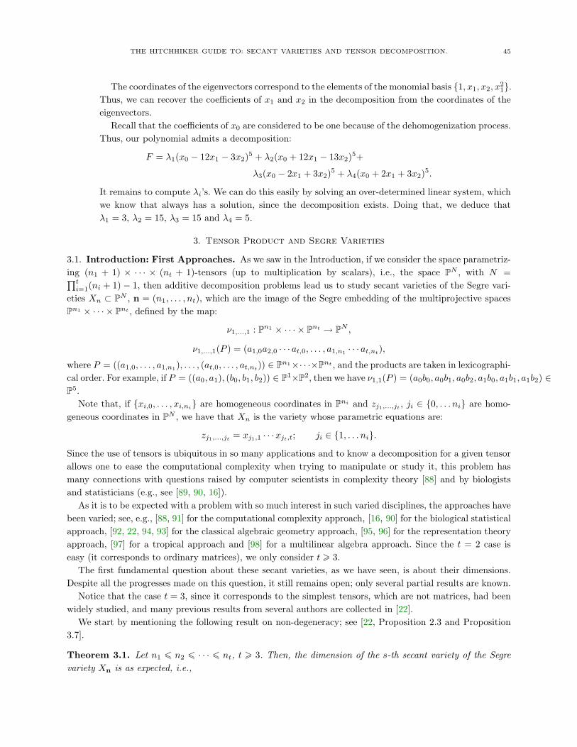
THE HITCHHIKER GUIDE TO: SECANT VARIETIES AND TENSOR DECOMPOSITION. 45
The coordinates of the eigenvectors correspond to the elements of the monomial basis {1, x1, x2, x21}.
Thus, we can recover the coefficients of x1 and x2 in the decomposition from the coordinates of theeigenvectors.
Recall that the coefficients of x0 are considered to be one because of the dehomogenization process.Thus, our polynomial admits a decomposition:
F = λ1(x0 − 12x1 − 3x2)5 + λ2(x0 + 12x1 − 13x2)5+
λ3(x0 − 2x1 + 3x2)5 + λ4(x0 + 2x1 + 3x2)5.
It remains to compute λi’s. We can do this easily by solving an over-determined linear system, whichwe know that always has a solution, since the decomposition exists. Doing that, we deduce thatλ1 = 3, λ2 = 15, λ3 = 15 and λ4 = 5.
3. Tensor Product and Segre Varieties
3.1. Introduction: First Approaches. As we saw in the Introduction, if we consider the space parametriz-ing (n1 + 1) × · · · × (nt + 1)-tensors (up to multiplication by scalars), i.e., the space PN , with N =∏ti=1(ni + 1) − 1, then additive decomposition problems lead us to study secant varieties of the Segre vari-
eties Xn ⊂ PN , n = (n1, . . . , nt), which are the image of the Segre embedding of the multiprojective spacesPn1 × · · · × Pnt , defined by the map:
ν1,...,1 : Pn1 × · · · × Pnt → PN ,
ν1,...,1(P ) = (a1,0a2,0 · · · at,0, . . . , a1,n1 · · · at,nt),
where P = ((a1,0, . . . , a1,n1), . . . , (at,0, . . . , at,nt)) ∈ Pn1×· · ·×Pnt , and the products are taken in lexicographi-cal order. For example, if P = ((a0, a1), (b0, b1, b2)) ∈ P1×P2, then we have ν1,1(P ) = (a0b0, a0b1, a0b2, a1b0, a1b1, a1b2) ∈P5.
Note that, if {xi,0, . . . , xi,ni} are homogeneous coordinates in Pni and zj1,...,jt , ji ∈ {0, . . . ni} are homo-geneous coordinates in PN , we have that Xn is the variety whose parametric equations are:
zj1,...,jt = xj1,1 · · ·xjt,t; ji ∈ {1, . . . ni}.
Since the use of tensors is ubiquitous in so many applications and to know a decomposition for a given tensorallows one to ease the computational complexity when trying to manipulate or study it, this problem hasmany connections with questions raised by computer scientists in complexity theory [88] and by biologistsand statisticians (e.g., see [89, 90, 16]).
As it is to be expected with a problem with so much interest in such varied disciplines, the approaches havebeen varied; see, e.g., [88, 91] for the computational complexity approach, [16, 90] for the biological statisticalapproach, [92, 22, 94, 93] for the classical algebraic geometry approach, [95, 96] for the representation theoryapproach, [97] for a tropical approach and [98] for a multilinear algebra approach. Since the t = 2 case iseasy (it corresponds to ordinary matrices), we only consider t 3.
The first fundamental question about these secant varieties, as we have seen, is about their dimensions.Despite all the progresses made on this question, it still remains open; only several partial results are known.
Notice that the case t = 3, since it corresponds to the simplest tensors, which are not matrices, had beenwidely studied, and many previous results from several authors are collected in [22].
We start by mentioning the following result on non-degeneracy; see [22, Proposition 2.3 and Proposition3.7].
Theorem 3.1. Let n1 ¬ n2 ¬ · · · ¬ nt, t 3. Then, the dimension of the s-th secant variety of the Segrevariety Xn is as expected, i.e.,
46 A. BERNARDI, E. CARLINI, M.V. CATALISANO, A. GIMIGLIANO, AND A. ONETO
dimσs(Xn) = s(n1 + n2 + · · ·+ nt + 1)− 1
if either:
• s ¬ n1 + 1; or• max{nt + 1, s} ¬
[n1+n2+···+nt+1
2
].
In the paper mentioned above, these two results are obtained in two ways. The first is via combinatorics onmonomial ideals in the multihomogeneous coordinate ring of Pn1×· · ·×Pnt : curiously enough, this correspondsto understanding possible arrangements of a set of rooks on an t-dimensional chessboard (corresponding tothe array representing the tensor). There is also a reinterpretation of these problems in terms of code theoryand Hamming distance (the so-called Hamming codes furnish nice examples of non-defective secants varietiesto Segre’s of type Pn × · · · × Pn).
Combinatorics turns out to be a nice, but limited tool for those questions. The second part of Theorem3.1 (and many other results that we are going to report) are obtained by the use of inverse systems andthe multigraded version of apolarity theory (recall Section 2.1.4 for the standard case, and we refer to[99, 100, 102, 101] for definitions of multigraded apolarity) or via Terracini’s lemma (see Lemma 2.13).
The idea behind these methods is to translate the problem of determining the dimension of σs(X), intothe problem of determining the multihomogeneous Hilbert function of a scheme Z ⊂ Pn1 × · · · × Pnt of sgeneric two-fat points in multi-degree 1 = (1, . . . , 1). We have that the coordinate ring of the multi-projectivespace Pn1×· · ·×Pnt is the polynomial ring S = k[x1,0, . . . , x1,n1 , . . . , xt,0, . . . , xt,nt ], equipped with the multi-degree given by deg(xi,j) = ei = (0, . . . , 1
i, . . . , 0). Then, the scheme Z is defined by a multi-homogeneous
ideal I = I(Z), which inherits the multi-graded structure. Hence, recalling the standard definition of Hilbertfunction (Definition 2.26), we say that the multi-graded Hilbert function of Z in multi-degree d = (d1, . . . , dt)is:
HF(Z; d) = dimk(S/I)d = dimk Sd − dimk Id.
3.2. The Multiprojective Affine Projective Method. We describe here a way to study the dimensionof σs(Xn) by studying the multi-graded Hilbert function of a scheme of fat points in multiprojective spacevia a very natural reduction to the Hilbert function of fat points in the standard projective space (of equaldimension).
We start recalling a direct consequence of Terracini’s lemma for any variety.Let Y ⊂ PN be a positive dimensional smooth variety, and let Z ⊂ Y be a scheme of s generic two-fat points,
i.e., a scheme defined by the ideal sheaf IZ = I2P1,Y
∩ · · · ∩ I2Ps,Y
⊂ OY , where the Pi’s are s generic pointsof Y defined by the ideal sheaves IPi,Y ⊂ OY , respectively. Since there is a bijection between hyperplanesof the space PN containing the linear space 〈TP1(Y ), . . . , TPs(Y )〉 and the elements of H0(Y, IZ(1)), we havethe following consequence of the Terracini lemma.
Theorem 3.2. Let Y be a positive dimensional smooth variety; let P1, . . . , Ps be generic points on Y ; andlet Z ⊂ Y be the scheme defined by I2
P1,Y∩ . . . ∩ I2
Ps,Y. Then,
dimσs(Y ) = dim〈TP1(Y ), . . . , TPs(Y )〉 = N − dimkH0(Y, IZ(1)).
Now, we apply this result to the case of Segre varieties; we give, e.g., [103] as the main reference. ConsiderPn := Pn1×· · ·×Pnt , and let Xn ⊂ PN be its Segre embedding given by OPn1 (1)⊗ . . .⊗OPnt (1). By applyingTheorem 3.2 and since the scheme Z ⊂ Xn corresponds to a scheme of s generic two-fat points in X, which,by a little abuse of notation, we call again Z, we get:
dimσs(Xn) = HF(Z,1)− 1.
THE HITCHHIKER GUIDE TO: SECANT VARIETIES AND TENSOR DECOMPOSITION. 47
Now, let n = n1 + · · ·+ nt, and consider the birational map:
Pn 99K An,
where: ([x1,0 : · · · : x1,n1 ], . . . , [xt,0, . . . , xt,nt ]
)
7→(x1,1x1,0
,x1,2x1,0
, . . . ,x1,n1x1,0
; x2,1x2,0, . . . ,
x2,n2x2,0
; . . . ; xt,1xt,0, . . . ,
xt,ntxt,0
).
This map is defined in the open subset of Pn given by {x1,0x2,0 · · ·xt,0 6= 0}.Now, let k[z0, z1,1, . . . , z1,n1 , z2,1, . . . , z2,n2 , . . . , zt,1, . . . , zt,nt ] be the coordinate ring of Pn, and consider
the embedding of An → Pn, whose image is the affine chart {z0 6= 0}. By composing the two maps above, weget:
ϕ : Pn 99K Pn,with: (
[x1,0 : · · · : x1,n1 ], . . . , [xt,0, . . . , xt,nt ])
7→[1 : x1,1x1,0
: x1,2x1,0: · · · : x1,n1x1,0
: x2,1x2,0: · · · : x2,n2x2,0
: · · · : xt,1xt,0: · · · : xt,ntxt,0
].
Let Z ⊂ X be a zero-dimensional scheme, which is contained in the affine chart {x0,1x0,2 · · ·x0,t 6= 0}, andlet Z ′ = ϕ(Z). We want to construct a scheme W ⊂ Pn such that HF(W ; d) = HF(Z; (d1, . . . , dt)), whered = d1 + . . .+ dt.
Let:Q0, Q1,1, . . . , Q1,n1 , Q2,1, . . . , Q2,n2 , Qt,1, . . . , Qt,nt
be the coordinate points of Pn. Consider the linear space Πi∼= Pni−1 ⊂ Pn, where Πi = 〈Qi,1, . . . , Qi,ni〉.
The defining ideal of Πi is:
I(Πi) = (z0, z1,1, . . . , z1,n1 ; . . . ; zi,1, . . . , zi,ni ; . . . ; zt,1, . . . , zt,nt) .
Let Wi be the subscheme of Pn denoted by (di − 1)Πi, i.e., the scheme defined by the ideal I(Πi)di−1. SinceI(Πi) is a prime ideal generated by a regular sequence, the ideal I(Πi)di−1 is saturated (and even primaryfor I(Πi)). Notice that Wi ∩Wj = ∅, for i 6= j. With this construction, we have the following key result.
Theorem 3.3. Let Z, Z ′, W1, . . . ,Wt be as above, and let W = Z ′ + W1 + · · · + Wt ⊂ Pn. Let I(W ) ⊂ S
and I(Z) ⊂ R be the ideals of W and Z, respectively. Then, we have, for all (d1, . . . , dt) ∈ Nt:
dimk I(W )d = dimk I(Z)(d1,...,dt),
where d = d1 + · · ·+ dt.
Note that when studying Segre varieties, we are only interested to the case (d1, . . . , dt) = (1, . . . , 1); but,in the more general case of Segre–Veronese varieties, we will have to look at Theorem 3.3 for any multidegree(d1, . . . , dt); see Section 4.2.
Note that the scheme W in Pn that we have constructed has two parts: the part W1 + · · · + Wt (whichwe shall call the part at infinity and we denote as W∞) and the part Z ′, which is isomorphic to our originalzero-dimensional scheme Z ⊂ X. Thus, if Z = ∅ (and hence, Z ′ = ∅), we obtain from the theorem that:
dimk I(W∞)d = dimk S(d1,...,dt), d = d1 + · · ·+ dt.
It follows that:
HF(W∞; d) =(d1 + · · ·+ dt + n
n
)−(d1 + n1
n1
)· · ·(dt + ntnt
).
With this observation made, the following corollary is immediate.
48 A. BERNARDI, E. CARLINI, M.V. CATALISANO, A. GIMIGLIANO, AND A. ONETO
Corollary 3.4. Let Z and Z ′ be as above, and write W = Z ′ +W∞. Then,
HF(W ; d) = HF(Z; (d1, . . . , dt)) + HF(W∞; d).
Eventually, when Z is given by s generic two-fat points in multi-projective space, we get the following.
Theorem 3.5. Let Z ⊂ X be a generic set of s two-fat points, and let W ⊂ Pn be as in the Theorem 3.3.Then, we have:
dimσs(Xn) = HF(Z, (1, . . . , 1))− 1 = N − dim I(W )t,
where N = Πti=1(1 + ni)− 1.
Therefore, eventually, we can study a projective scheme W ⊂ Pn, which is made of a union of generictwo-fat points and of fat linear spaces. Note that, when n1 = . . . = nt = 1, then also W is a scheme offat points.
3.3. The Balanced Case. One could try to attack the problem starting with a case, which is in a sensemore “regular”, i.e., the “balanced” case of n1 = · · · = nt, t 3. Several partial results are known, andthey lead Abo, Ottaviani and Peterson to propose, in their lovely paper [92], a conjecture, which states thatthere are only a finite number of defective Segre varieties of the form Pn × · · · × Pn, and their guess is thatσ4(P2 × P2 × P2) and σ3(P1 × P1 × P1 × P1) are actually the only defective cases (as we will see later, this isjust part of an even more hazardous conjecture; see Conjecture 3.9).
In the particular case of n1 = · · · = nt = 1, the question has been completely solved in [104], supportingthe above conjecture.
Theorem 3.6. [104] Let t, s ∈ N, t 3. Let X1 be the Segre embedding of P1 × · · · × P1, (t-times). Thedimension of σs(X1) ⊂ PN , with N = 2t − 1, is always as expected, i.e.,
dimσs(X) = min{N, s(t+ 1)− 1},
except for t = 4, s = 3. In this last case, dimσ3(X) = 13, instead of 14.
The method that has been used to compute the multi-graded Hilbert function for schemes of two-fat pointswith generic support in multi-projective spaces is based first on the procedure described on the multiprojectiveaffine projective method explained in the previous section, which brings to the study of the standard Hilbertfunction of the schemes W ⊂ Pt. Secondly, the problem of determining the dimension of I(W )t can be attackedby induction, via the powerful tool constituted by the differential Horace method, created by Alexander andHirschowitz; see Section 2.2.2. This is used in [104] together with other “tricks”, which allow one to “move”on a hyperplane some of the conditions imposed by the fat points, analogously as we have described in theexamples in Section 2.2.2. These were the key ingredients to prove Theorem 3.6.
The only defective secant variety in the theorem above is made by the second secant variety of P1 × P1 ×P1×P1 ⊂ P15, which, instead of forming a hypersurface in P15, has codimension two. Via Theorem 3.5 above,this is geometrically related to a configuration of seven fat points; more precisely, in this case, the scheme Wof Theorem 3.5 is union of three two-fat points and four three-fat ones (see also Theorem 3.3 for a detaileddescription of W ). These always lie on a rational normal curve in P4 (see, e.g., Theorem 1.18 of [1]) and donot have the expected Hilbert function in degree four, by the result in [105].
For the general “balanced” case Pn × · · · × Pn, the following partial result is proven in [92].
Theorem 3.7. Let Xn be the Segre embedding of Pn × · · · × Pn (t times), t 3. Let st and et be defined by:
st =⌊
(n+ 1)t
nt+ 1
⌋and et ≡ st mod (n+ 1) with et ∈ {0, . . . , n}.
Then:
THE HITCHHIKER GUIDE TO: SECANT VARIETIES AND TENSOR DECOMPOSITION. 49
• if s ¬ st − et, then σs(X) has the expected dimension;• if s st − et + n+ 1, then σs(X) fills the ambient space.
In other words, if st = q(n + 1) + r, with 1 ¬ r ¬ n, then σs(Xn) has the expected dimension both fors (q + 1)(n + 1) and for s ¬ q(n + 1), but if n + 1 divides st, then σs(X) has the expected dimension forany s.
Other known results in the “balanced” case are the following:
• σ4(P2 × P2 × P2) is defective with defect δ4 = 1; see [21].• Pn × Pn × Pn is never defective for n 3; see [106];• Pn × Pn × Pn × Pn for 2 ¬ n ¬ 10 is never defective except at most for s = 100 and n = 8 or fors = 357 and n = 10; see [107].
3.4. The General Case. When we drop the balanced dimensions request, not many defective cases areactually known. For example:
• P2 × P3 × P3 is defective only for s = 5, with defect δ4 = 1; see [92];• P2 × Pn × Pn with n even is defective only for s = 3n
2 + 1 with defect δs = 1; see [22, 94].• P1 × P1 × Pn × Pn is defective only for s = 2n+ 1 with defect δ2n+1 = 1; see [92].
However, when taking into consideration cases where the ni’s are far from being equal, we run into another“defectivity phenomenon”, known as “the unbalanced case”; see [22, 108].
Theorem 3.8. Let Xn be the Segre embedding of Pn1×· · ·×Pnt×Pn ⊂ PM , with M = (n+1)Πti=1(ni+1)−1.
Let N = Πti=1(ni + 1)− 1, and assume n > N −
∑ti=1 ni + 1. Then, σs(X) is defective for:
N −t∑i=1
ni + 1 < s ¬ min{n;N},
with defect equal to δs(X) = s2 − s(N −∑ti=1 ni + 1).
The examples described above are the few ones for which defectivities of Segre varieties are known. There-fore, the following conjecture has been stated in [92], where, for n1 ¬ n2 ¬ . . . ¬ nt, it is proven for s ¬ 6.
Conjecture 3.9. The Segre embeddings of Pn1 × · · · .× Pnt , t 3, are never defective, except for:
• P1 × P1 × P1 × P1, for s = 3, with δ3 = 1;• P2 × P2 × P2, for s = 4, with δ4 = 1;• the “unbalanced case”;• P2 × P3 × P3, for s = 5, with δ5 = 1;• P2 × Pn × Pn, with n even, for s = 3n
2 + 1, with δs = 1);• P1 × P1 × Pn × Pn, for s = 2n+ 1, with δ2n+1 = 1).
4. Other Structured Tensors
There are other varieties of interest, parametrizing other “structured tensors”, i.e., tensors that havedetermined properties. In all these cases, there exists an additive decomposition problem, which can begeometrically studied similarly as we did in the previous sections. In this section, we want to present someof these cases.
In particular, we consider the following structured tensors:
(1) skew-symmetric tensors, i.e., v1 ∧ . . . ∧ vk ∈∧k
V ;(2) decomposable partially-symmetric tensors, i.e., Ld11 ⊗ . . .⊗ L
dtt ∈ Sd1V ∗1 ⊗ · · · ⊗ SdtV ∗t ;
50 A. BERNARDI, E. CARLINI, M.V. CATALISANO, A. GIMIGLIANO, AND A. ONETO
(3) d-powers of linear forms, i.e., homogeneous polynomials Ld11 · · ·Ldtt ∈ SdV ∗, for any partition d =
(d1, . . . , dt) ` d;(4) reducible forms, i.e., F1 · · ·Ft ∈ SdV ∗, where deg(Fi) = di, for any partition d = (d1, . . . , dt) ` d;(5) powers of homogeneous polynomials, i.e., Gk ∈ SdV ∗, for any k|d;
4.1. Exterior Powers and Grassmannians. Denote by G(k, n) the Grassmannian of k-dimensional linearsubspaces of Pn ∼= PV , for a fixed n+1 dimensional vector space V . We consider it with the embedding givenby its Plucker coordinates as embedded in PNk , where Nk =
(n+1k
)− 1.
The dimensions of the higher secant varieties to the Grassmannians of lines, i.e., for k = 1, are well known;e.g., see [7], [109] or [110]. The secant variety σs(Gr(1, n)) parametrizes all (n+ 1)× (n+ 1) skew-symmetricmatrices of rank at most 2s.
Theorem 4.1. We have that σs(G(1, n)) is defective for s < bn+12 c with defect equal to δs = 2s(s− 1).
For k 2, not many results can be found in the classical or contemporary literature about this problem;e.g., see [109, 110, 111]. However, they are sufficient to have a picture of the whole situation. Namely, thereare only four other cases that are known to be defective (e.g., see [110]), and it is conjectured in [112] thatthese are the only ones. This is summarized in the following conjecture:
Conjecture 4.2 (Baur–Draisma–de Graaf, [112]). Let k 2. Then, the secant variety σs(G(k, n)) has theexpected dimension except for the following cases:
actual codimension expected codimensionσ3(G(2, 6)) 1 0σ3(G(3, 7)) 20 19σ4(G(3, 7)) 6 2σ4(G(2, 8)) 10 8
In [112], they proved the conjecture for n ¬ 15 (the case n ¬ 14 can be found in [113]). The conjecturehas been proven to hold for s ¬ 6 (see [111]) and later for s ¬ 12 in [114].
A few more results on non-defectivity are proven in [111, 110]. We summarize them in the following.
Theorem 4.3. The secant variety σs(G(k, n)) has the expected dimension when:
• k 3 and ks ¬ n+ 1,• k = 2, n 9 and s ¬ s1(n) or s s2(n),
where:
s1(n) =⌊n2
18− 20n
27+
28781
⌋+⌊
6n− 139
⌋and s2(n) =
⌈n2
18− 11n
27+
4481
⌉+⌈
6n− 139
⌉;
in the second case, σs(G(2, n)) fills the ambient space.
Other partial results can be found in [114], while in [115], the following theorem can be found.
Definition 4.4. Given an integer m 2, we define a function hm : N→ N as follows:
• hm(0) = 0;• for any k 1, write k+ 1 = 2λ1 + 2λ2 + . . .+ 2λ` + ε, for a suitable choice of λ1 > λ2 > . . . > λ` 1,ε ∈ {0, 1}, and define:
hm(k) := mλ1−1 +mλ2−1 + . . .+mλ`−1.
In particular, we get hm(2k) = hm(2k − 1), and h2(k) = bk+12 c.
THE HITCHHIKER GUIDE TO: SECANT VARIETIES AND TENSOR DECOMPOSITION. 51
Theorem 4.5 (Theorem 3.5.1 of [115, ]). Assume that k 2, and set:
α :=⌊n+ 1k + 1
⌋.
If either:
• n k2 + 3k + 1 and h ¬ αhα(k − 1);
or:
• n < k2 + 3k + 1, k is even, and h ¬ (α− 1)hα(k − 1) + hα(n− 2− αr);
or:
• n < k2 + 3k + 1, r is odd, and:
h ¬ (α− 1)hα(k − 2) + hα(min{n− 3− α(k − 1), r − 2}),
then, G(k, n) is not (h+ 1)-defective.
This results strictly improves the results in [111] for k 4, whenever (k, n) 6= (4, 10), (5, 11); see [115].
Notice that, if we let R∧(k, n) be the generic rank with respect to G(k, n), i.e., the minimum s such thatσs(G(k, n)) = PNk , we have that the results above give that, asymptotically:
R∧(2, n) ∼ n2
18.
A better asymptotic result can be found in [115].Finally, we give some words concerning the methods involved. The approach in [110] uses Terracini’s lemma
and an exterior algebra version of apolarity. The main idea there is to consider the analog of the perfect pairinginduced by the apolarity action that we have seen for the symmetric case in the skew-symmetric situation;see Section 2.1.4. In fact, the pairing considered here is:
k∧V ×
n−k∧V →
n∧V ' k,
induced by the multiplication in∧V , and it defines the apolarity of a subspace Y ⊂ V of dimension k to
be Y ⊥ := {w ∈∧n−k
V |w ∧ v = 0∀ v ∈ Y }. Now, one can proceed in the same way as the symmetric case,namely by considering a generic element of the Grassmannian G(k, n) and by computing the tangent space atthat point. Then, its orthogonal, via the above perfect pairing, turns out to be, as in the symmetric case, thedegree n−k part of an ideal, which is a double fat point. Hence, in [110], the authors apply Terracini’s lemmato this situation in order to study all the known defective cases and in other various cases. Notice that theabove definition of skew-symmetric apolarity works well for computing the dimension of secant varieties toGrassmannians since it defines the apolar of a subspace that is exactly what is needed for Terracini’s lemma,but if one would like to have an analogous definition of apolarity for skew symmetric tensors, then there area few things that have to be done. Firstly, one needs to extend by linearity the above definition to all theelements of
∧kV . Secondly, in order to get the equivalent notion of the apolar ideal in the skew symmetric
setting, one has to define the skew-symmetric apolarity in any degree ¬ d. This is done in [116], where alsothe skew-symmetric version of the apolarity lemma is given. Moreover, in [116], one can find the classificationof all the skew-symmetric-ranks of any skew-symmetric tensor in
∧3 Cn for n ¬ n (the same classificationcan actually be found also in [118, 117]), together with algorithms to get the skew-symmetric-rank and theskew-symmetric decompositions for any for those tensors (as far as we know, this is new).
Back to the results on dimensions of secant varieties of Grassmannians: in [112], a tropical geometryapproach is involved. In [111], as was done by Alexander and Hirshowitz for the symmetric case, the authorsneeded to introduce a specialization technique, by placing a certain number of points on sub-Grassmannians
52 A. BERNARDI, E. CARLINI, M.V. CATALISANO, A. GIMIGLIANO, AND A. ONETO
and by using induction. In this way, they could prove several non-defective cases. Moreover, in the same work,invariant theory was used to describe the equation of σ3(G(2, 6)), confirming the work of Schouten [119], whofirstly proved that it was defective by showing that it is a hypersurface (note that by parameter count, it isexpected to fill the ambient space). Lascoux [120] proved that the degree of Schouten’s hypersurface is seven.In [92], with a very clever idea, an explicit description of this degree seven invariant was found by relatingits cube to the determinant of a 21× 21 symmetric matrix.
Eventually, in [115], the author employed a new method for studying the defectivity of varieties based onthe study of osculating spaces.
4.2. Segre–Veronese Varieties. Now, we consider a generalization of the apolarity action that we haveseen in both Section 2 and Section 3 to the multi-homogeneous setting; see [99, 100, 102, 101]. More precisely,fixing a set of vector spaces V1, . . . , Vt of dimensions n1 + 1, . . . , nt + 1, respectively, and positive integersd1, . . . , dt, we consider the space of partially-symmetric tensors:
Sd1V ∗1 ⊗ . . .⊗ SdtV ∗t .
The Segre–Veronese variety parametrizes decomposable partially-symmetric tensors, i.e., it is the image ofthe embedding:
νn,d : P(S1V ∗1 )× . . .× P(S1V ∗t ) −→ P(Sd1V ∗1 ⊗ . . .⊗ SdtV ∗t )
([L1], . . . , [Lt]) 7→[Ld11 ⊗ . . .⊗ L
dtt
],
where, for short, we denote n = (n1, . . . , nt), d = (d1, . . . , dt).More geometrically, the Segre–Veronese variety is the image of the Segre–Veronese embedding:
νn,d : Pn := Pn1 × . . .× Pnt −→ PN , where N =t∏i=1
(di + nini
)− 1,
given by OPn(d) := OPn1 (d1) ⊗ . . . ⊗ OPnt (dt), that is via the forms of multidegree (d1, . . . , dt) of themultigraded homogeneous coordinate ring:
R = k[x1,0, . . . , x1,n1 ;x2,0, . . . , x2,n2 ; . . . ;xt,0, . . . , xt,nt ].
For instance, if n = (2, 1), d = (1, 2) and P = ([a0 : a1 : a2], [b0 : b1]) ∈ P2 × P1, we have νn,d(P ) = [a0b20 :
a0b0b1 : a0b21 : a1b
20 : a1b0b1 : a1b
21 : a2b
20 : a2b0b1 : a2b
21], where the products are taken in lexicographical
order. We denote the embedded variety νn,d(Pn) by Xn,d. Clearly, for t = 1, we recover Veronese varieties,while for (d1, . . . , dt) = (1, . . . , 1), we get the Segre varieties.
The corresponding additive decomposition problem is as follows.
Problem 3. Given a partially-symmetric tensor T ∈ Sd1V ∗1 × . . . × PSdtV ∗t or, equivalently, a multi-homogeneous polynomial T ∈ R of multidegree d, find the smallest possible length r of an expressionT =
∑ri=1 L
d1i,1 ⊗ . . .⊗ L
dti,t.
As regards the generic tensor, a possible approach to this problem mimics what has been done for Segre andVeronese varieties. One can use Terracini’s lemma (Lemma 2.13 and Theorem 3.2), as in [22, 103], to translatethe problem of determining the dimensions of the higher secant varieties of Xn,d into that of calculating thevalue, at d = (d1, . . . , dt), of the Hilbert function of generic sets of two-fat points in Pn. Then, by usingthe multiprojective affine projective method introduced in Section 3.2, i.e., by passing to an affine chart inPn and then homogenizing in order to pass to Pn, with n = n1 + · · · + nt, this last calculation amounts tocomputing the Hilbert function in degree d = d1 + · · ·+ dn for the subscheme W ⊂ Pn; see Theorem 3.3.
There are many scattered results on the dimension of σs(Xn,d), by many authors, and very few generalresults. One is the following, which generalizes the “unbalanced” case considered for Segre varieties; see[108, 92].
THE HITCHHIKER GUIDE TO: SECANT VARIETIES AND TENSOR DECOMPOSITION. 53
Theorem 4.6. Let X = X(n1,...,nt,n),(d1,...,dt,1) be the Segre–Veronese embedding:
Pn1 × . . .× Pnt × Pn (d1,...,dt,1)−→ X ⊂ PM , with M = (n+ 1)
(t∏i=1
(ni + didi
))− 1.
Let N = Πti=1
(ni+didi
)− 1, then, for N −
∑ti=1 ni + 1 < s ¬ min{n,N}, the secant variety σs(X) is defective
with δs(X) = s2 − s(N −∑ti=1 ni + 1).
When it comes to Segre–Veronese varieties with only two factors, there are many results by many authors,which allow us to get a quite complete picture, described by the following conjectures, as stated in [121].
Conjecture 4.7. Let X = X(m,n),(a,b), then X is never defective, except for:
• b = 1, m 2, and it is unbalanced (as in the theorem above);• (m,n) = (1, n), (a, b) = (2d, 2);• (m,n) = (3, 4), (a, b) = (2, 1);• (m,n) = (2, n), (a, b) = (2, 2);• (m,n) = (2, 2k + 1), k 1, (a, b) = (1, 2);• (m,n) = (1, 2), (a, b) = (1.3);• (m,n) = (2, 2), (a, b) = (2, 2);• (m,n) = (3, 3), (a, b) = (2, 2);• (m,n) = (3, 4), (a, b) = (2, 2).
Conjecture 4.8. Let X = X(m,n),(a,b), then for (a, b) (3, 3), X is never defective.
The above conjectures are based on results that can be found in [123, 131, 93, 128, 99, 122, 126, 130, 112,129, 134, 125, 124, 132, 133, 127, 121].
For the Segre embeddings of many copies of P1, we have a complete result. First, in [99] and in [130], thecases of two and three copies of P1, respectively, were completely solved.
Theorem 4.9. Let X = X(1,1),(a,b), a ¬ b. Then, X is never defective, except for (a, b) = (2, 2d); in thiscase, σ2d+1(X) is defective with δ2d+1 = 1.
Theorem 4.10. Let X = X(1,1,1),(a,b,c), a ¬ b ¬ c; then X is never defective, except for:
• (a, b, c) = (1, 1, 2d); in this case, σ2d+1(X) is defective with δ2d+1 = 1;• (a, b, c) = (2, 2, 2); here, σ7(X) is defective, and δ7 = 1.
In [135] the authors, by using an induction approach, whose basic step was Theorem 3.6 about the Segrevarieties X1 [104], concluded that there are no other defective cases except for the previously-known ones.
Theorem 4.11. Let X = X(1,...,1),(a1,...,ar). Then, X is never defective, except for:
• X(1,1),(2,2d) (Theorem 4.9);• X(1,1,1),(1,1,2d) and X(1,1,1),(2,2,2) (Theorem 4.10);• X(1,1,1,1),(1,1,1,1) (Theorem 3.6).
For several other partial results on the defectivity of certain Segre–Veronese varieties, see, e.g., [99, 136,133, 115], and for an asymptotic result about non-defective Segre–Veronese varieties, see [137, 115].
4.3. Tangential and Osculating Varieties to Veronese Varieties. Another way of generalizing whatwe saw in Section 2 for secants of Veronese Varieties Xn,d is to work with their tangential and osculatingvarieties.
54 A. BERNARDI, E. CARLINI, M.V. CATALISANO, A. GIMIGLIANO, AND A. ONETO
Definition 4.12. Let Xn,d ⊂ PN be a Veronese variety. We denote by τ(Xn,d) the tangential variety ofXn,d, i.e., the closure in PN of the union of all tangent spaces:
τ(Xn,d) =⋃
P∈Xn,d
TP (Xn,d) ⊂ PN .
More in general, we denote by Ok(Xn.d) the k-th osculating variety of Xn,d, i.e., the closure in PN of theunion of all k-th osculating spaces:
Ok(Xn,d) =⋃
P∈Xn,d
OkP (Xn,d) ⊂ PN .
Hence, τ(Xn,d) = O1(Xn,d).
These varieties are of interest also because the space Ok(Xn,d) parametrizes a particular kind of form.Indeed, if the point P = [Ld] ∈ Xn,d ⊂ PSd, then the k-th osculating space OkP (Xn,d) correspond to linearspace
{[Ld−kG] | G ∈ Sk
}. Therefore, the corresponding additive decomposition problem asks the following.
Problem 4. Given a homogeneous polynomial F ∈ k[x0, . . . , xn], find the smallest length of an expressionF =
∑ri=1 L
d−ki Gi, where the Li’s are linear forms and the Gi’s are forms of degree k.
The type of decompositions mentioned in the latter problem have been called generalized additive de-composition in [25] and in [30]. In the special case of k = 1, they are a particular case of the so-calledChow–Waring decompositions that we treat in full generality in Section 4.4. In this case, the answer toProblem 4 is called (d− 1, 1)-rank, and we denote it by R(d−1,1)(F ).
Remark 4.13. Given a family of homogeneous polynomials F = {F1, . . . , Fm}, we define the simultaneousrank of F the smallest number of linear forms that can be used to write a Waring decomposition of allpolynomials of F .
Now, a homogeneous polynomial F ∈ SdV can be seen as a partially-symmetric tensor in S1V ⊗ Sd−1V
via the equality:
F =1d
n∑i=0
xi ⊗∂F
∂xi.
From this expression, it is clear that a list of linear forms that decompose simultaneously all partial derivativesof F also decompose F , i.e., the simultaneous rank of the first partial derivatives is an upper bound of thesymmetric-rank of F . Actually, it is possible to prove that for every homogeneous polynomial, this is anequality (e.g., see [138] (Section 1.3) or [139] (Lemma 2.4)). For more details on relations between simultaneousranks of higher order partial derivatives and partially-symmetric-ranks, we refer to [139].
Once again, in order to answer the latter question in the case of the generic polynomial, we study thesecant varieties to the k-th osculating variety of Xn,d. In [21], the dimension of σs(τ(Xn,d)) is studied (k = 1case). Via apolarity and inverse systems, with an analog of Theorem 3.2, the problem is again reduced to thecomputation of the Hilbert function of some particular zero-dimensional subschemes of Pn; namely,
dimσs(τ(Xn,d)) = dimk(Ld−11 , . . . , Ld−1
s , Ld−21 M1, . . . , L
d−2s Ms)d − 1 =
= HF(Z, d)− 1,
where L1, . . . , Ls,M1, . . . ,Ms are 2s generic linear forms in k[x0, . . . , xn], while HF(Z, d) is the Hilbert func-tion of a scheme Z, which is the union of s generic (2, 3)-points in Pn, which are defined as follows.
Definition 4.14. A (2, 3)-point is a zero-dimensional scheme in Pn with support at a point P and whoseideal is of type I(P )3 + I(`)2, where I(P ) is the homogeneous ideal of P and ` ⊂ Pn is a line through P
defining ideal I(`).
THE HITCHHIKER GUIDE TO: SECANT VARIETIES AND TENSOR DECOMPOSITION. 55
Note that when we say that Z is a scheme of s generic (2, 3)-points in Pn, we mean that I(Z) = I(Q1) ∩. . . ∩ I(Qs), where the Qi’s are (2, 3)-points, i.e., I(Qi) = I(Pi)3 + I(`i)2, such that P1, . . . Ps are genericpoints in Pn, while `1, . . . , `s are generic lines passing though P1, . . . , Ps, respectively.
By using the above fact, in [21], several cases where σs(τ(Xn,d)) is defective were found, and it wasconjectured that these exceptions were the only ones. The conjecture has been proven in a few cases in [22](s ¬ 5 and n s + 1) and in [140] (n = 2, 3). In [71], it was proven for n ¬ 9, and moreover, it was proventhat if the conjecture holds for d = 3, then it holds in every case. Finally, by using this latter fact, Abo andVannieuwenhoven completed the proof of the following theorem [141].
Theorem 4.15. The s-th secant variety σs(τ(Xn,d)) of the tangential variety to the Veronese variety hasdimension as expected, except in the following cases:
(1) d = 2 and 2 ¬ 2s < n;(2) d = 3 and n = 2, 3, 4.
As a direct corollary of the latter result, we obtain the following answer to Problem 4 in the case of genericforms.
Corollary 4.16. Let F ∈ Sd be a generic form. Then,
R(d−1,1)(F ) =
⌈ (n+dn
)2n+ 1
⌉,
except for:
(1) d = 2, where R(d−1,1)(F ) =⌊n2
⌋+ 1;
(2) d = 3 and n = 2, 3, 4, where R(d−1,1)(F ) =⌈
(n+dn )2n+1
⌉+ 1.
The general case of σs(Ok(Xn.d)) is studied in [143, 71, 144, 142]. Working in analogy with the casek = 1, the dimension of σs(Ok(Xn,d) is related to the Hilbert function of a certain zero-dimensional schemeZ = Z1 ∪ · · · ∪ Zs, whose support is a generic union of points P1, . . . , Ps ∈ Pn, respectively, and such that,for each i = 1, . . . , s, we have that (k + 1)Pi ⊂ Zi ⊂ (k + 2)Pi.
As one of the manifestations of the ubiquity of fat points, the following conjecture describes the conditionsfor the defect of this secant variety in terms of the Hilbert function of fat points:
Conjecture 4.17 ([71] (Conjecture 2a)). The secant variety σs(Ok(Xn,d)) is defective if and only if either:
(1) h1(IX(d)) > max{0,degZ −(d+nn
)}, or
(2) h0(IT (d)) > max{0,(d+nn
)− degZ},
where X is a generic union of s (k + 1)-fat points and T is a generic union of (k + 2)-fat points.
In [144, 142], the conjecture is proven for n = 2, s ¬ 9, and in [71] for n = 2 and any s.
4.4. Chow–Veronese Varieties. Let d = (d1, . . . , dt) be a partition of a positive integer d, i.e., d1 . . . dtare positive integers, which sum to d. Then, we consider the following problem.
Let S =⊕
d∈N Sd be a polynomial ring in n+ 1 variables.
Problem 5. Given a homogeneous polynomial F ∈ Sd, find the smallest length of an expression F =∑ri=1 L
d1i,1 · · ·L
dti,t, where Li,j’s are linear forms.
The decompositions considered in the latter question are often referred to as Chow–Waring decompositions.We call the answer to Problem 5 as the d-rank of F , and we denote it by Rd(F ).
56 A. BERNARDI, E. CARLINI, M.V. CATALISANO, A. GIMIGLIANO, AND A. ONETO
In this case, the summands are parametrized by the so-called Chow–Veronese variety, which is given bythe image of the embedding:
νd : PS1 × . . .× PS1 −→ PSd,([L1], . . . , [Lt]) 7→
[Ld11 · · ·L
dtt
].
We denote by Xd the image νd(Pn). Notice that this map can be seen as a linear projection of the Segre–Veronese variety Xn,d ⊂ P(Sd1⊗ . . .⊗Sdt), for n = (n, . . . , n), under the map induced by the linear projectionof the space of partially-symmetric tensors Sd1 ⊗ . . . ⊗ Sdt on the totally symmetric component Sd. Onceagain, we focus on the question posed in Problem 5 in the case of a generic polynomial, for which we studydimensions of secant varieties to Xd.
In the case of d = (d− 1, 1), we have that Xd coincides with the tangential variety of the Veronese varietyτ(Xn,d), for which the problem has been completely solved, as we have seen in the previous section (Theorem4.15).
The other special case is given by d = (1, . . . , 1), for d 3. In this case, Xd has been also referred to asthe Chow variety or as the variety of split forms or completely decomposable forms. After the first work byArrondo and Bernardi [74], Shin found the dimension of the second secant variety in the ternary case (n = 2)[145], and Abo determined the dimensions of higher secant varieties [146]. All these cases are non-defective.It is conjectured that varieties of split forms of degree d 3 are never defective. New cases have been recentlyproven in [147, 148].
The problem for any arbitrary partition d has been considered in [149]. Dimensions of all s-th secantvarieties for any partition haves been computed in the case of binary forms (n = 1). In a higher number ofvariables, the dimensions of secant line varieties (s = 2) and of higher secant varieties with s ¬ 2
⌊n3
⌋have
been computed. This was done by using the classical Terracini’s lemma (Lemma 2.13) in order to obtain anice description of the generic tangent space of the s-th secant variety. In the following example, we explainhow the binary case could be treated.
Example 4.18. If P = [Ld11 · · ·Ldtt ] ∈ Xd, then it is not difficult to prove (see Proposition 2.2 in [149, ])
that:
TPXd = P ((IP )d) , with d = d1 + . . .+ dt
where IP = (Ld1−11 Ld22 · · ·L
dtt , L
d11 L
d2−12 · · ·Ldtt , . . . , L
d11 L
d22 · · ·L
dt−1t ).
In the particular case of binary forms, some more computations show that actually, TPXd = P ((I ′P )d),where I ′P is the principal ideal (Ld1−1
1 · · ·Ldt−1t ). In this way, by using Terracini’s lemma, we obtain that, if
Q is a generic point on the linear span of s generic points on Xd, then:
TQσs(Xd) = P(
(Ld1−11,1 · · ·Ldt−1
1,t , . . . , Ld1−1s,1 · · ·Ldt−1
s,t )d),
where Li,j ’s are generic linear forms. Now, in order to compute the dimension of this tangent space, we canstudy the Hilbert function of the ideal on the right-hand side. By semicontinuity, we may specialize to thecase Li,1 = . . . = Li,t, for any i = 1, . . . , s. In this way, we obtain a power ideal, i.e., an ideal generated bypowers of linear forms, whose Hilbert function is prescribed by Froberg–Iarrobino’s conjecture; see Remark2.33. Now, since in [150], the authors proved that the latter conjecture holds in the case of binary forms, i.e.,the Hilbert function of a generic power ideal in two variables is equal to the right-hand side of (2.13), we canconclude our computation of the dimension of the secant variety of Xd in the binary case. This is the wayTheorem 3.1 in [149, ] was proven.
In the following table, we resume the current state-of-the-art regarding secant varieties and Chow–Veronesevarieties.
THE HITCHHIKER GUIDE TO: SECANT VARIETIES AND TENSOR DECOMPOSITION. 57
d s d n References dimσs(Xd)(d− 1, 1) any any any [141] non-defective, except for
(1) d = 2 and 2 ¬ 2s < n;(2) d = 3 and n = 2, 3, 4.
(1, . . . , 1) d > 2 3(s− 1) < n [74] non-defectiveany any 2 [146] non-defective, except for cases abovesome numerical constraints [146, 148]
any any any 1 [149] non-defective, except for cases above2 any any
¬ 2⌊n3
⌋any any
4.5. Varieties of Reducible Forms. In 1954, Mammana [151] considered the variety of reducible planecurves and tried to generalize previous works by, among many others, C. Segre, Spampinato and Bordiga.More recently, in [147], the authors considered the varieties of reducible forms in full generality.
Let d = (d1, . . . , dt) ` d be a partition of a positive integer d, i.e., d1 . . . dt are positive integers,which sum up to d and t 2. Inside the space of homogeneous polynomials of degree d, we define the varietyof d-reducible forms as:
Yd = {[F ] ∈ PSd | F = G1 · · ·Gt, where deg(Gi) = di},
i.e., the image of the embedding:
ψd : PSd1 × . . .× PSdt −→ PSd,(G1, . . . , Gt) 7→ Gd11 · · ·G
dtt .
Clearly, if d = 2, then d = (1, 1), and Y(1,1) is just the Chow variety X(1,1). In general, we may see Ydas the linear projection of the Segre variety Xm inside P(Sd1 ⊗ · · · ⊗ Sdt), where m = (m1, . . . ,mt) withmi =
(di+nn
)− 1. Note that, if d,d′ are two partitions of d such that d can be recovered from d′ by grouping
and summing some of entries, then we have the obvious inclusion Yd′ ⊂ Yd. Therefore, if we define the varietyof reducible forms as the union over all possible partitions d ` d of the varieties Yd, we can actually write:
Y =b d2 c⋃k=1
Y(d−k,k) ⊂ PSd.
In terms of additive decompositions, the study of varieties of reduced forms and their secant varieties isrelated to the notion of the strength of a polynomial, which was recently introduced by T. Ananyan and M.Hochster [152] and then generalized to any tensor in [153].
Problem 6. Given a homogeneous polynomial F ∈ Sd, find the smallest length of an expression F =∑ri=1Gi,1Gi,2, where 1 ¬ deg(Gi,j) ¬ d− 1.
The answer to Problem 6 is called the strength of F , and we denote it by S(F ).In [147], the authors gave a conjectural formula for the dimensions of all secant varieties σs(Yd) of the
variety of d-reducible forms for any partition d (see Conjecture 1.1 in [147, ]), and they proved it undercertain numerical conditions (see Theorem 1.2 in [147, ]). These computations have been made by using theclassical Terracini’s lemma and relating the dimensions of these secants to the famous Froberg’s conjectureon the Hilbert series of generic forms.
The variety of reducible forms is not irreducible and the irreducible component with biggest dimension isthe one corresponding to the partition (d − 1, 1), i.e., dimY = dimY(d−1,1). Higher secant varieties of thevariety of reducible forms are still reduced, but understanding which is the irreducible component with thebiggest dimension is not an easy task. In Theorem 1.5 of [147, ], the authors proved that, if 2s ¬ n− 1, then
58 A. BERNARDI, E. CARLINI, M.V. CATALISANO, A. GIMIGLIANO, AND A. ONETO
the biggest irreducible component of σs(Y ) is σs(Y(d−1,1), i.e., dimσs(Y ) = dimσs(Y(d−1,1)), and togetherwith the aforementioned Theorem 1.2 of [147, ], this allows us to compute the dimensions of secant varietiesof varieties of reducible forms and answer Problem 6 under certain numerical restrictions (see Theorem 7.4[147, ]).
In conclusion, we have that Problem 6 is answered in the following cases:
(1) any binary form (n = 2), where S(F ) = 1,since every binary form is a product of linear forms;
(2) generic quadric (d = 2), where S(F ) =⌊n2
⌋+ 1,
since it forces d = (1, 1), which is solved by Corollary 4.16 (2);(3) generic ternary cubic (n = 2, d = 3), where S(F ) = 2,
since Y(2,1) is seven-dimensional and non-degenerate inside P9 = PS3, then σ2(Y(2,1)) cannot beeight-dimensional; otherwise, we get a contradiction by one of the classical Palatini’s lemmas, whichstates that if dimσs+1(X) = dimσs(X) + 1, then σs+1(X) must be a linear space [2].
4.6. Varieties of Powers. Another possible generalization of the classical Waring problem for forms is givenby the following.
Problem 7. Given a homogeneous polynomial F ∈ Sd and a positive divisor k > 1 of d, find the smallestlength of an expression F =
∑ri=1G
ki .
The answer to Problem 7 is called the k-th Waring rank, or simply k-th rank, of F , and we denote itRkd(F ). In this case, we need to consider the variety of k-th powers, i.e.,
Vk,d = {[Gk] ∈ PSd | G ∈ Sd/k}.
That is, the variety obtained by considering the composition:
(4.1) π ◦ νk : PSd/k → PSk(Sd/k) 99K PSd,
where:
(1) if W = Sd/k, then νk is the k-th Veronese embedding of PW in PSkW ;(2) if we consider the standard monomial basis wα = xα of W , i.e., |α| = d/k, then π is the linear
projection from PSkW to PSd induced by the substitution wα 7→ xα. In particular, we have that thecenter of the projection π is given by the homogeneous part of degree k of the ideal of the Veronesevariety νd(Pn).
Problem 7 was considered by Froberg, Shapiro and Ottaviani [154]. Their main result was that, if F is generic,then:
(4.2) Rkd(F ) ¬ kn,
i.e., the kn-th secant variety of Vk,d fills the ambient space. This was proven by Terracini’s lemma. Indeed,for any G,H ∈ Sd/k, we have that:
ddt
∣∣∣∣t=0
(G+ tH)k = kGk−1H;
therefore, we obtain that:
T[Gk]Vk,d = P(〈[Gk−1H] | H ∈ Sd/k〉
),
and, by Terracini’s lemma (Lemma 2.13), if Q is a generic point on 〈[Gk1 ], . . . , [Gks ]〉, where the Gi’s are genericforms of degree d/k, then:
(4.3) TQσsVk,d = P((Gk−1
1 , . . . , Gk−1s )d
).
THE HITCHHIKER GUIDE TO: SECANT VARIETIES AND TENSOR DECOMPOSITION. 59
In [154, Theorem 9], the authors showed that the family:
Gi1,...,in = (x0 + ξi1x1 + . . .+ ξinxn)d/k ∈ Sd/k, for i1, . . . , in ∈ {0, . . . , k − 1},
where ξk = 1, is such that:(Gk−1
1 , . . . , Gk−1s )d = Sd.
In this way, they showed that σkn(Vk,d) fills the ambient space. A remarkable fact with the upperbound (4.2)is that it is independent of the degree of the polynomial, but it only depends on the power k. Now, the naive
lower bound due to parameter counting is⌈
dimSddimSd/k
⌉=⌈
(n+dn )(n+d/kn )
⌉, which tends to kn when d runs to infinity.
In conclusion, we obtain that the main result of [154] is resumed as follows.
Theorem 4.19 ([154, Theorem 4]). Let F be a generic form of degree d in n+ 1 variables. Then,
Rkd(F ) ¬ kn.
If d� 0, then the latter bound is sharp.
This result gives an asymptotic answer to Problem 7, but, in general, it is not known for which degree dthe generic k-th Waring rank starts to be equal to kn, and it is not known what happens in lower degrees.
We have explained in (4.1) how to explicitly see the variety of powers Vk,d as a linear projection of aVeronese variety XN,k = νk(PN ), where N =
(n+d/kn
)− 1. It is possible to prove that σ2(XN,k) does not
intersect the base of linear projection, and therefore, Vk,d is actually isomorphic to XN,k. Unfortunately,higher secant varieties intersect non-trivially the base of the projection, and therefore, their images, i.e., thesecant varieties of the varieties of powers, are more difficult to understand. However, computer experimentssuggest that the dimensions are preserved by the linear projection; see [155] (Section 4) for more details aboutthese computations (a Macaulay2 script with some examples is available in the ancillary files of the arXivversion of [155]). In other words, it seems that we can use the Alexander–Hirschowitz theorem to computethe dimensions of secant varieties of varieties of powers and provide an answer to Problem 7. More on thisconjecture is explained in [155].
Conjecture 4.20 ([155] (Conjecture 1.2)). Let F be a generic form of degree d in n+ 1 variables. Then,
Rkd(F ) =
{min{s 1 | s
(n+d/2n
)−(s2
)(n+dn
)} for k = 2;
min{s 1 | s(n+d/kn
)(n+dn
)} for k 3.
Remark 4.21. The latter conjecture claims that for k 3, the correct answer is given by the direct parametercount. For k = 2, we have that secant varieties are always defective. This is analogous to the fact that secantvarieties to the two-fold Veronese embeddings are defective. Geometrically, this is motivated by Terracini’slemma and by the fact that:
T[G2]V2,d ∩ T[H2]V2,d = [GH],
and not empty, as expected.
Example 4.22. Here, we explain how the binary case can be treated; see [155, Theorem 2.3]. By (4.3),the computation of the dimension of secant varieties of varieties of powers reduces to the computation ofdimensions of homogeneous parts of particular ideals, i.e., their Hilbert functions. This relates Problem 7 tosome variation of Froberg’s conjecture, which claims that the ideal (Gk1 , . . . , G
ks), where the Gi’s are generic
forms of degrees at least two, has Hilbert series equal to the right-hand side of (2.13); see [156]. In the caseof binary forms, by semicontinuity, we may specialize the Gi’s to be powers of linear forms. In this way, wemay employ the result of [150], which claims that power ideals in two variables satisfy Froberg–Iarrobino’sconjecture, i.e., (2.13) is actually an equality, and we conclude the proof of Conjecture 4.20 in the case ofbinary forms.
60 A. BERNARDI, E. CARLINI, M.V. CATALISANO, A. GIMIGLIANO, AND A. ONETO
By using an algebraic study on the Hilbert series of ideals generated by powers of forms, we have a completeanswer to Problem 7 in the following cases (see [155]):
(1) binary forms (n = 1), where:
Rkd(F ) =
⌈d+ 1d/k + 1
⌉;
(2) ternary forms as sums of squares (n = 2, k = 2), where:
R2d(F ) =
⌈ (d+2
2
)(d/2+2
2
)⌉ ,except for d = 1, 3, 4, where R2
d(F ) =⌈
(d+22 )(d/2+22 )
⌉+ 1.;
(3) quaternary forms as sums of squares (n = 3, k = 2), where:
R2d(F ) =
⌈ (d+3
3
)(d/2+3
3
)⌉ ,except for d = 1, 2, where R2
d(F ) =⌈
(d+33 )(d/2+33 )
⌉+ 1.
5. Beyond Dimensions
We want to present here, as a natural final part of this work, a list of problems about secant varietiesand decomposition of tensors, which are different from merely trying to determine the dimensions of thevarieties σs(X) for the various X we have considered before. We will consider problems such as determiningmaximal possible ranks, finding bounds or exact values on ranks of given tensor, understanding the set ofall possible minimal decompositions of a given tensor, finding equations for the secant varieties or studyingwhat happens when working over R. The reader should be aware of the fact that there are many very difficultopen problems around these questions.
5.1. Maximum Rank. A very difficult and still open problem is the one that in the Introduction we havecalled the “little Waring problem”. We recall it here.
Which is the minimum integer r such that any form can be written as a sum of r pure powersof linear forms?
This corresponds to finding the maximum rank of a form of certain degree d in a certain number n+ 1 ofvariables.
To our knowledge, the best general achievement on this problem is due to Landsberg and Teitler, who in[76, Proposition 5.1] proved that the rank of a degree d form in n + 1 variables is smaller than or equal to(n+dd
)− n. Unfortunately, this bound is sharp only for n = 1 if d 2 (binary forms); in fact, for example, if
n = 2 and d = 3, 4, then the maximum ranks are known to be 5 <(2+3
2
)− 3 = 7 and 7 <
(2+42
)− 4 = 11,
respectively; see [28, Theorem 40 and Theorem 44]. Another general bound has been obtained by Jelisiejew[158], who proved that, for F ∈ Sdkn+1, we have Rsym(F ) ¬
(n+d−1d−1
)−(n+d−5d−3
). Again, this bound is not
sharp for n 2. Another remarkable result is the one due to Blekherman and Teitler, who proved in [157,Theorem 1] that the maximum rank is always smaller than or equal to twice the generic rank.
Remark 5.1. The latter inequality, which has a very short and elegant proof, holds also between maximaland generic X-ranks with respect to any projective variety X.
In a few cases in small numbers of variables and small degrees, exact values of maximal ranks have beengiven. We resume them in the following table.
THE HITCHHIKER GUIDE TO: SECANT VARIETIES AND TENSOR DECOMPOSITION. 61
d n Maximal Rank Ref.binary forms any 1 d classical, [159]
quadrics 2 any n+ 1 classicalplane cubics 3 2 5 [160, 76]
plane quartics 4 2 7 [162, 161]plane quintics 5 2 10 [163, 164]cubic surfaces 3 3 7 [160]
cubic hypersurfaces 3 any ¬⌊d2+6d+1
4
⌋[165]
We want to underline the fact that it is very difficult to find examples of forms having high rank, in thesense higher than the generic rank. Thanks to the complete result on monomials in [166] (see Theorem 5.15),we can easily see that in the case of binary and ternary forms, we can find monomials having rank higherthan the generic one. However, for higher numbers of variables, monomials do not provide examples of formsof high rank. Some examples are given in [164], and the spaces of forms of high rank are studied from ageometric point of view in [167].
5.2. Bounds on the Rank. In the previous subsection, we discussed the problem of finding the maximalrank of a given family of tensors. However, for a given specific tensor T , it is more interesting, and relevant,to find explicit bounds on the rank of T itself. For example, by finding good lower and upper bounds on therank of T , one can try to compute actually the rank of T itself, but usually, the maximal rank is going to betoo large to be useful in this direction.
One typical approach to find upper bounds is very explicit: by finding a decomposition of T . In the caseof symmetric tensors, that is in the case of homogeneous polynomials, the apolarity lemma (Lemma 2.80) isan effective tool to approach algebraically the study of upper bounds: by finding the ideal of a reduced setof points X inside F⊥, we bound the rank of F from above by the cardinality of X.
Example 5.2. For F = x0x1x2, in standard notation, we have F⊥ = (y20 , y
21 , y
23), and we can consider the
complete intersection set of four reduced points X whose defining ideal is (y21 − y2
0 , y22 − y2
0), and thus, therank of F is at most four. Analogously, if F = x0x
21x
32, we have F⊥ = (y2
0 , y31 , y
43), and we can consider the
complete intersection of 12 points defined by (y31 − y3
0 , y42 − y4
0).
Other upper bounds have been given by using different notions of rank.
Definition 5.3. We say that a scheme Z ⊂ PN is curvilinear if it is a finite union of schemes of theform OCi,Pi/m
eiPi
, for smooth points Pi on reduced curves Ci ⊂ PN . Equivalently, the tangent space at eachconnected component of Z supported at the Pi’s has Zariski dimension ¬ 1. The curvilinear rank Rcurv(F )of a degree d form F in n+ 1 variables is:
Rcurv(F ) := min {deg(Z) | Z ⊂ Xn,d, Z curvilinear, [F ] ∈ 〈Z〉} .
With this definition, in [168, Theorem 1], it is proven that the rank of an F ∈ Sdkn+1 is bounded by(Rcurv(F )−1)d+ 2−Rcurv(F ). This result is sharp if Rcurv(F ) = 2, 3; see [28, Theorem 32 and Theorem 37].
Another very related notion of rank is the following; see [169, 82].
Definition 5.4. We define the smoothable rank of a form F ∈ Sdkn+1 as:
Rsmooth(F ) := min
{deg(Z)
∣∣∣ Z is a limit of smooth schemes Zi such thatZ,Zi ⊂ Xn,d, are zero-dim schemes with deg(Zi) = deg(Z),
and [F ] ∈ 〈Z〉
}.
In [168] (Section 2), it is proven that if F is a ternary form of degree d, then Rsym(F ) ¬ (Rsmooth(F )−1)d.We refer to [82] for a complete analysis on the relations between different notions of ranks.
62 A. BERNARDI, E. CARLINI, M.V. CATALISANO, A. GIMIGLIANO, AND A. ONETO
The use of the apolarity lemma (Lemma 2.80) to obtain lower bounds to the symmetric-rank of a homo-geneous polynomial was first given in [170].
Theorem 5.5 ([170, Proposition 1]). If the ideal F⊥ is generated in degree t and X is a finite scheme apolarto F , that is IX ⊂ F⊥, then:
1t
degF⊥ ¬ degX.
This result is enough to compute the rank of the product of variables.
Example 5.6. For F = x0x1x2, Theorem 5.5 yields:
12
8 ¬ degX.
If we assume X to be reduced, i.e., degX = |X|, by the apolarity lemma, we get Rsym(F ) 4, and thus, byExample 5.2, the rank of F is equal to four. However, for the monomial x0x
21x
32, we get the lower bound of
six, which does not allow us to conclude the computation of the rank, since Example 5.2 gives us 12 as theupper bound.
To solve the latter case, we need a more effective use of the apolarity lemma in order to produce a betterlower bound for the rank; see [166, 171].
Theorem 5.7 ([171] (Corollary 3.4)). Let F be a degree d form, and let e > 0 be an integer. Let I be anyideal generated in degree e, and let G be a general form in I. For s� 0, we have:
Rsym(F ) 1e
s∑i=0
HF(R/(F⊥ : I + (G)), i
).
A form for which there exists a positive integer e such that the latter lower bound is actually sharp is callede-computable; see [171]. Theorem 5.7 was first presented in [166] in the special case of e = 1: this was thekey point to prove Theorem 5.15 on the rank of monomials, by showing that monomials are one-computable.In order to give an idea of the method, we give two examples: in the first one, we compute the rank ofx0x
21x
32 by using one-computability, while in the second one, we give an example in which it is necessary to
use two-computability; see [166, 171].
Example 5.8. Consider again F = x0x21x
32. We use Theorem 5.7 with e = 1, G = y0 and I = (y0). Note
that:F⊥ : I + (G) = (y2
0 , y31 , y
42) : (y0) + (y0) = (y0, y
31 , y
42).
This yields to:
Rsym(F ) s∑i=0
HF(R/(y0, y
31 , y
42), i
)= 12,
since HS(R/(y0, y31 , y
42), z) = 1 + 2z + 3z2 + 3z3 + 2z4 + z5. Hence, by using Example 5.2, we conclude that
the rank of F is actually 12.
Example 5.9. Consider the polynomial:
F = x110 − 22x9
0x21 + 33x7
0x41 − 22x9
0x22 + 396x7
0x21x
22 − 462x5
0x41x
22+
33x70x
42 − 462x5
0x21x
42 + 385x3
0x41x
42,
,
we show that F is two-computable and Rsym(F ) = 25. By direct computation, we get:
F⊥ = ((y20 + y2
1 + y22)2, G1, G2),
where G1 = y51 + y2(y2
0 + y21 + y2
2)2 and G2 = y52 + y0(y2
0 + y21 + y2
2)2.
THE HITCHHIKER GUIDE TO: SECANT VARIETIES AND TENSOR DECOMPOSITION. 63
Hence, by (5.7), we get:
Rsym(F ) 12
∞∑i=0
HF (T/(F⊥ : (y20 + y2
1 + y22) + (y2
0 + y21 + y2
2)), i) = 25.
Moreover, the ideal (G1, G2) ⊂ F⊥ is the ideal of 25 distinct points, and thus, the conclusion follows. It canbe shown that F is not one-computable; see [171] (Example 4.23).
Another way to find bounds on the rank of a form is by using the rank of its derivatives. A first easy boundon the symmetric-rank of a homogeneous polynomial F ∈ k[x0, . . . , xn] (where k is a characteristic zero field)is directly given by the maximum between the symmetric-ranks of its derivatives; indeed, if F =
∑ri=1 L
di ,
then, for any j = 0, . . . , n,
(5.1)∂F
∂xj=
r∑i=1
∂Ldi∂xj
= (d− 1)r∑i=1
∂Li∂xj
Ld−1i .
A more interesting bound is given in [172].
Theorem 5.10 ([172, Theorem 3.2]). Let 1 ¬ p ¬ n be an integer, and let F ∈ k[x0, . . . , xn] be a form,where k is a characteristic zero field. Set Fk = ∂F
∂xk, for 0 ¬ k ¬ n. If:
rksym(F0 +n∑k=1
λkFk) m,
for all λk ∈ k, and if the forms F1, F2, . . . , Fp are linearly independent, then:
rksym(F ) m+ p.
The latter bound was lightly improved in [173, Theorem 2.3].Formula (5.1) can be generalized to higher order differentials. As a consequence, for any G ∈ SjV ∗, with
1 ¬ j ¬ d − 1, we have that Rsym(F ) Rsym(G ◦ F ), and in particular, if F ∈ 〈Ld1, . . . , Ldr〉, we have thatG ◦F ∈ 〈Ld−j1 , . . . , Ld−jr 〉. Since this holds for any G ∈ SjV ∗, we conclude that the image of the (j, d− j)-thcatalecticant matrix is contained in 〈Ld−j1 , . . . , Ld−jr 〉. Therefore,
(5.2) Rsym(F ) dimk(Imm Catj,d−j(F )) = rk Catj,d−j(F ).
The latter bound is very classical and goes back to Sylvester. By using the geometry of the hypersurfaceV (F ) in Pn, it can be improved; see [76].
Theorem 5.11 ([76, Theorem 1.3]). Let F be a degree d form with n+1 essential variables. Let 1 ¬ j ¬ d−1.Use the convention that dim ∅ = −1. Then, the symmetric-rank of F is such that:
Rsym(F ) rk Catj,d−j(F ) + dim Σj(F ) + 1,
where Catj,d−j(F ) is the (j, d− j)-th catalecticant matrix of F and:
Σj(F ) ={P ∈ V (F ) ⊂ PV :
∂αF
∂xα(P ) = 0, ∀|α| ¬ j
}.
The latter result has been used to find lower bounds on the rank of the determinant and the permanentof the generic square matrix; see [76] (Corollary 1.4).
The bound (5.2) given by the ranks of catalecticant matrices is a particular case of a more general fact,which holds for general tensors.
64 A. BERNARDI, E. CARLINI, M.V. CATALISANO, A. GIMIGLIANO, AND A. ONETO
Given a tensor T ∈ V1 ⊗ . . .⊗ Vd, there are several ways to view it as a linear map. For example, we can“reshape” it as a linear map V ∗i → V1 ⊗ . . .⊗ Vi ⊗ . . .⊗ Vd, for any i, or as V ∗i ⊗ V ∗j → V1 ⊗ . . .⊗ Vi ⊗ . . .⊗Vj ⊗ . . .⊗ Vd, for any i 6= j, or more in general, as:
(5.3) V ∗i1 ⊗ V∗i2 ⊗ . . .⊗ V
∗is → V1 ⊗ . . .⊗ Vi1 ⊗ . . .⊗ Vis ⊗ . . .⊗ Vd,
for any choice of i1, . . . , is. All these ways of reshaping the tensor are called flattenings. Now, if T is a tensorof rank r, then all its flattenings have (as matrices) rank at most r. In this way, the ranks of the flatteningsgive lower bounds for the rank of a tensor, similarly as the ranks of catalecticant matrices gave lower boundsfor the symmetric-rank of a homogeneous polynomial.
We also point out that other notions of flattening, i.e., other ways to construct linear maps starting from agiven tensor, have been introduced in the literature, such as Young flattenings (see [85]) and Koszul flattenings(see [84]). These were used to find equations of certain secant varieties of Veronese and other varieties andto provide algebraic algorithms to compute decompositions.
We conclude this section with a very powerful method to compute lower bounds on ranks of tensors: theso-called substitution method. In order to ease the notation, we report the result in the case T ∈ V1⊗V2⊗V3,with dimk Vi = ni. For a general result, see [175] (Appendix B).
Theorem 5.12 (The substitution method [175] (Appendix B) or [174] (Section 5.3)). Let T ∈ V1⊗ V2⊗ V3.Write T =
∑n1i=1 ei ⊗ Ti, where the ei’s form a basis of V1 and the Ti’s are the corresponding “slices” of the
tensor. Assume that Mn1 6= 0. Then, there exist constants λ1, . . . , λn1−1 such that the tensor:
T ′ =n1−1∑i=1
ei ⊗ (Ti − λiTn1) ∈ kn1−1 ⊗ V2 ⊗ V3,
has rank at most R(T )− 1. If Tn1 is a matrix of rank one, then equality holds.
Roughly speaking, this method is applied in an iterative way, with each of the Vi’s playing the role of V1
in the theorem, in order to reduce the tensor to a smaller one whose rank we are able to compute. Since, inthe theorem above, R(T ) R(T ′) + 1, at each step, we get a plus one on the lower bound. For a completedescription of this method and its uses, we refer to [174] (Section 5.3).
A remarkable use of this method is due to Shitov, who recently gave counterexamples to very interestingconjectures such as Comon’s conjecture, on the equality between the rank and symmetric-rank of a symmetrictensor, and Strassen’s conjecture, on the additivity of the tensor rank for sums of tensors defined over disjointsubvector spaces of the tensor space.
We will come back with more details on Strassen’s conjecture, and its symmetric version, in the nextsection. We spend a few words more here on Comon’s conjecture.
Given a symmetric tensor F ∈ SdV ⊂ V ⊗d, we may regard it as a tensor, forgetting the symmetries, andwe could ask for its tensor rank, or we can take into account its symmetries and consider its symmetric-rank.Clearly,
(5.4) R(F ) ¬ Rsym(F ).
The question raised by Comon asks if whether such an inequality is actually an equality. Affirmative answerswere given in several cases (see [179, 176, 180, 178, 177]). In [181], Shitov found an example (a cubic in 800variables) where the inequality (5.4) is strict. As the author says, unfortunately, no symmetric analogs ofthis substitution method are known. However, a possible formulation of such analogs, which might lead to asmaller case where (5.4) is strict, was proposed.
THE HITCHHIKER GUIDE TO: SECANT VARIETIES AND TENSOR DECOMPOSITION. 65
Conjecture 5.13 ([181] (Conjecture 7)). Let F,G ∈ S = k[x0, . . . , xn] of degree d, d− 1, respectively. Let Lbe a linear form. Then,
Rsym(F + LG) d+ minL′∈S1
Rsym(F + L′G).
Remark 5.14. A symmetric tensor F ∈ SdV can be viewed as a partially-symmetric tensor in Sd1V ⊗ . . .⊗SdmV , for any d = (d1, . . . , dm) ∈ Nm such that d1 + . . . + dm = d. Moreover, if d′ = (d′1, . . . , d
′m′) ∈ Nm′ is
a refinement of d, i.e., there is some grouping of the entries of d′ to get d, then we have:
(5.5) Rsym(F ) Rd(F ) Rd′(F ),
which is a particular case of (5.4). In the recent paper [139], the authors investigated the partially-symmetricversion of Comon’s question, i.e., the question if, for a given F , (5.5) is an equality or not. Their approachconsisted of bounding from below the right-hand side of (5.5) with the simultaneous rank of its partialderivatives of some given order and then studying the latter by using classical apolarity theory (see alsoRemark 4.13). If such a simultaneous rank coincides with the symmetric-rank of F , then also all intermediateranks are the same. In particular, for each case in which Comon’s conjecture is proven to be true, thenalso all partially-symmetric tensors coincide. For more details, we refer to [139], where particular families ofhomogeneous polynomials are considered.
5.3. Formulae for Symmetric Ranks. In order to find exact values of the symmetric-rank of a givenpolynomial, we can use one of the available algorithms for rank computations; see Section 2.3. However, aswe already mentioned, the algorithms will give an answer only if some special conditions are satisfied, andthe answer will be only valid for that specific form. Thus, having exact formulae working for a family of formsis of the utmost interest.
Formulae for the rank are usually obtained by finding an explicit (a posteriori sharp) upper bound andthen by showing that the rank cannot be less than the previously-found lower bound.
An interesting case is the one of monomials. The lower bound of (5.7) is used to obtain a rank formulafor the complex rank of any monomial, similarly as in Example 5.8; i.e., given a monomial F = xα, whoseexponents are increasingly ordered, we have that F⊥ = (yα0+1
0 , . . . , yαn+1n ), and then, one has to:
(1) first, as in Example 5.2, exhibit the set of points apolar to F given by the complete intersection(yα11 − y
α10 , . . . , yαnn − y
α00 ); this proves that the right-hand side of (5.6) is an upper bound for the
rank;(2) second, as in Example 5.8, use Theorem 5.7 with e = 1 and G = y0 to show that the right-hand side
of (5.6) is a lower bound for the rank.
Theorem 5.15 ([166, Proposition 3.1]). Let 1 ¬ α0 ¬ α1 . . . ¬ αn. Then,
(5.6) Rsym(xα) =1
α0 + 1
n∏i=0
(αi + 1).
Another relevant type of forms for which we know the rank is the one of reduced cubic forms. Thereducible cubics, which are not equivalent to a monomial (up to change of variables), can be classified intothree canonical forms. The symmetric complex rank for each one was computed, as the following resultsummarizes: the first two were first presented in [76], while the last one is in [172]. In particular, for all threecases, we have that the lower bound given by Theorem 5.10 is sharp.
Theorem 5.16 ([172, Theorem 4.5]). Let F ∈ C[x0, . . . , xn] be a form essentially involving n + 1 vari-ables, which is not equivalent to a monomial. If F is a reducible cubic form, then one and only one of thefollowing holds:
66 A. BERNARDI, E. CARLINI, M.V. CATALISANO, A. GIMIGLIANO, AND A. ONETO
(1) F is equivalent to:
x0(x20 + x2
1 + . . .+ x2n),
and Rsym(F ) = 2n.(2) F is equivalent to:
x0(x21 + x2
2 + . . .+ x2n),
and Rsym(F ) = 2n.(3) F equivalent to:
x0(x0x1 + x2x3 + x24 + . . .+ x2
n),
and Rsym(F ) = 2n+ 1.
Another way to find formulae for symmetric-ranks relies on a symmetric version of Strassen’s conjectureon tensors. In 1973, Strassen formulated a conjecture about the additivity of the tensor ranks [183], i.e., giventensors Ti, . . . , Ts in V ⊗d defined over disjoint subvector spaces, then,
R(s∑i=1
Ti) =s∑i=1
R(Ti).
After a series of positive results (see, e.g., [186, 185, 184]), Shitov gave a proof of the existence of a counter-example to the general conjecture in the case of tensors of order three [187]. Via a clever use of the substitutionmethod we introduced in the previous section, the author described a way to construct a counter-example,but he did not give an explicit one.
However, as the author mentioned is his final remarks, no counter example is known for the symmetricversion of the conjecture that goes as follows: given homogeneous polynomials F1, . . . , Fs in different sets ofvariables, then:
Rsym(s∑i=1
Fi) =s∑i=1
Rsym(Fi).
In this case, Strassen’s conjecture is known to be true in a variety of situations. The case of sums of coprimemonomials was proven in [166, Theorem 3.2] via apolarity theory by studying the Hilbert function of theapolar ideal of F =
∑si=1 Fi. Indeed, it is not difficult to prove that:
F⊥ =s⋂i=1
F⊥i + (Fi + λi,jFj : i 6= j),(5.7)
where the λi,j ’s are suitable coefficients.
In this way, since apolar ideals of monomials are easy to compute, it is possible to express explicitly also theapolar ideal of a sum of coprime monomials. Therefore, the authors applied an analogous strategy as the oneused for Theorem 5.15 (by using more technical algebraic computations) to prove that Strassen’s conjectureholds for sums of monomials.
In [188], the authors proved that Strassen’s conjecture holds whenever the summands are in either one ortwo variables. In [171, 173], the authors provided conditions on the summands to guarantee that additivity ofthe symmetric-ranks holds. For example, in [173], the author showed that whenever the catalecticant bound(5.2) (or the lower bound given by Theorem 5.11) is sharp for all the Fi’s, then Strassen’s conjecture holds,and the corresponding bound for
∑si=1 Fi is also sharp.
A nice list of cases in which Strassen’s conjecture holds was presented in [171]. This was done againby studying the Hilbert function of the apolar ideal of F =
∑si=1 Fi, computed as described in (5.7), and
employing the bound given by Theorem 5.7.
THE HITCHHIKER GUIDE TO: SECANT VARIETIES AND TENSOR DECOMPOSITION. 67
Theorem 5.17 ([171, Theorem 6.1]). Let F = F1 + . . . + Fm, where the degree d forms Fi are in differentsets of variables. If, for i = 1, . . . ,m, each Fi is of one of the following types:
• Fi is a monomial;• Fi is a form in one or two variables;• Fi = xa0(xb1 + . . .+ xbn) with a+ 1 b;• Fi = xa0(xb1 + xb2);• Fi = xa0(xb0 + . . .+ xbn) with a+ 1 b;• Fi = xa0(xb0 + xb1 + xb2);• Fi = xa0G(x1, . . . , xn) where G⊥ = (H1, . . . ,Hm) is a complete intersection and a ¬ degHi;• Fi is a Vandermonde determinant;
then Strassen’s conjecture holds for F .
5.4. Identifiability of Tensors. For simplicity, in this section we work on the field C of the complexnumbers. Let us consider tensors in V = Cn1+1⊗ . . .⊗Cnd+1. A problem of particular interest when studyingminimal decompositions of tensors is to count how many there are.
Problem 8. Suppose a given tensor T ∈ V has rank r, i.e., it can be written as T =⊕r
i=1 v1i ⊗. . .⊗vdi . When
is it that such a decomposition is unique (up to permutation of the summands and scaling of the vectors)?
This problem has been studied quite a bit in the last two centuries (e.g., see [191, 189, 12, 190]), and itis also of interest with respect to many applied problems (e.g., see [192, 193, 194]). Our main references forthis brief exposition are [195, 196].
Let us begin with a few definitions.
Definition 5.18. A rank-r tensor T ∈ V is said to be identifiable over C if its presentation T =⊕r
i=1 v1i ⊗
. . .⊗ vdi is unique (up to permutations of the summands and scaling of the vectors).
It is interesting to study the identifiability of a generic tensor of given shape and rank.
Definition 5.19. We say that tensors in V are r-generically identifiable over C if identifiability over C holdsin a Zariski dense open subset of the space of tensors of rank r. Moreover, we say that the tensors in V aregenerically identifiable if they are rg-generically identifiable, where rg denotes the generic rank in V.
Let us recall that the generic rank for tensors V is the minimum value for which there is a Zariski opennon-empty set U of V where each point represents a tensor with rank ¬ rg; see Section 3. Consideringn = (n1, . . . , nd), let Xn ⊂ PV be the Segre embedding of Pn1 × . . . × Pnd . As we already said previously,if rg is the generic rank for tensors in V, then σrg (Xn) is the first secant variety of Xn, which fills theambient space. Therefore, to say that the tensors in V are generically identifiable over C amounts to sayingthe following: let rg be the generic rank with respect to the Segre embedding Xn in PV; then, for the genericpoint [T ] ∈ PV, there exists a unique Pr−1, which is rg-secant to Xn in rg distinct points and passes through[T ]. The rg points of Xn gives (up to scalar) the rg summands in the unique (up to permutation of summands)minimal decomposition of the tensor T .
When σr(Xn) 6= PV, i.e., the rank r is smaller than the generic one (we can say that r is sub-generic),then we have that the set of tensors T ∈ V with rank r is r-generically identifiable over C if there is an openset U of σr(Xn) such that for the points [T ] in U , there exists a unique Pr−1, which is r-secant in r distinctpoints to Xn and passes through [T ].
Obviously, the same problem is interesting also when treating symmetric or skew-symmetric tensors, i.e.,when n1 = . . . = nd = n and T ∈ Sd(Cn+1) ⊂ V or T ∈
∧d(Cn+1). From a geometric point of view, in these
68 A. BERNARDI, E. CARLINI, M.V. CATALISANO, A. GIMIGLIANO, AND A. ONETO
cases, we have to look at Veronese varieties or Grassmannians, respectively, and their secant varieties, as wehave seen in the previous sections.
Generic identifiability is quite rare as a phenomenon, and it has been largely investigated; in particular, werefer to [200, 198, 199, 197, 201, 202, 189, 12]. As an example of how generic identifiability seldom presentsitself, we can consider the case of symmetric tensors.
It is classically known that there are three cases of generic identifiability, namely:
• binary forms of odd degree (n = 1 and d = 2t+ 1), where the generic rank is t+ 1 [190];• ternary quintics (n = 2 and d = 5), where the generic rank is seven [191];• quaternary cubics (n = 3 and d = 3), where the generic rank is five [190].
Recently, Galuppi and Mella proved that these are the only generically identifiable cases when consideringsymmetric-ranks of symmetric tensors; see [203].
When we come to partially-symmetric tensors (which are related to Segre–Veronese varieties, as we de-scribed in Section 4.2), a complete classification of generically-identifiable cases is not known, but it is knownthat it happens in the following cases; see [204].
• Sd1C2⊗. . .⊗SdtC2, with d1 ¬ . . . dt and d1+1 rg, where rg is the generic partially-symmetric-rank,i.e., forms of multidegree (d1, . . . , dt) in t sets of two variables; here, the generic partially-symmetric-rank is t+ 1 [205];
• S2Cn+1 ⊗ S2Cn+1, i.e., forms of multidegree (2, 2) in two sets of n + 1 variables; her,e the genericpartially-symmetric-rank is n+ 1 [206];
• S2C3⊗S2C3⊗S2C3⊗S2C3, i.e., forms of multidegree (2, 2, 2, 2) in four sets of three variables; here,the generic partially-symmetric-rank is four (this is a classical result; see also [204]);
• S2C3⊗S3C3, i.e., forms of multidegree (2, 3) in two sets of three variables; here, the generic partially-symmetric-rank is four [207];
• S2C3 ⊗ S2C3 ⊗ S4C3, i.e., forms of multidegree (2, 2, 4) in three sets of three variables; here, thegeneric partially-symmetric-rank is seven [204].
When considering r-generically identifiable tensors for sub-generic rank, i.e., for r < rg, things changecompletely, in as much as we do expect r-generically-identifiability in this case. Again, the symmetric caseis the best known; in [202, Theorem 1.1], it was proven that every case where r is a sub-generic rank andσr(Xn,d) has the expected dimension for the Veronese variety Xn,d, r-generically identifiability holds withthe only following exceptions:
• S6C3, i.e., forms of degree six in three variables, having rank nine;• S4C4, i.e., forms of degree four in four variables, having rank eight;• S3C6, i.e., forms of degree three in six variables, having rank nine.
In all the latter cases, the generic forms have exactly two decompositions.Regarding generic identifiability for skew-symmetric tensors, there are not many studies, and we refer to
[208].It is quite different when we are in the defective cases, namely, when we want to study r-generic iden-
tifiability and the r-th secant variety is defective. In this case, non-identifiability is expected; in particular,we will have that the number of decompositions for the generic tensor parametrized by a point of σr(Y ) isinfinite.
5.5. Varieties of Sums of Powers. Identifiability deals with the case in which tensors have a unique (upto permutation of the summands) decomposition. When the decomposition is not unique, what can we sayabout all possible decompositions of the given tensor? In the case of symmetric tensors, that is homogeneous
THE HITCHHIKER GUIDE TO: SECANT VARIETIES AND TENSOR DECOMPOSITION. 69
polynomial, an answer is given by studying varieties of sums of powers, the so-called VSP, defined by Ranestadand Schreyer in [209].
Definition 5.20. Let F be a form in n+ 1 variables having Waring rank r, and let HilbrPn be the Hilbertscheme of r points in Pn; we define:
VSP(F, r) = {X = {P1, . . . , Pr} ∈ HilbrPn : IX = ℘1 ∩ . . . ∩ ℘r ⊂ F⊥}.
For example, when identifiability holds, VSP is just one single point. It is interesting to note that, evenfor forms having generic rank, the corresponding VSP might be quite big, as in the case of binary forms ofeven degree.
Using Sylvester’s algorithm we have a complete description of VSP for binary forms, and it turns out tobe always a linear space.
Example 5.21. Consider the binary form F = x20x
21. Since F⊥ = (y3
0 , y31), by Sylvester’s algorithm, we have
that the rank of F is three. Moreover, by the apolarity lemma, we have that VSP(F, 3) is the projectivizationof the vector space W = 〈y3
0 , y31〉 because the generic form in W has three distinct roots.
In general, the study of VSPsis quite difficult, but rewarding: VSPs play an important role in classificationwork by Mukai see [212, 210, 211]. For a review of the case of general plane curves of degree up to ten, that isfor general ternary forms of degree up to ten, a complete description is given in [209], including results fromMukai and original results. We summarize them in the following.
Theorem 5.22 ([209, Theorem 1.7]). Let F ∈ SdC3 be a general ternary cubic with d = 2t − 2, 2 ¬ t ¬ 5,then:
VSP(F,
(t+ 1
2
))' G(t, V, η) = {E ∈ G(t, V ) | ∧2 E ⊂ η}
where V is a 2t + 1-dimensional vector space and η is a net of alternating forms η : Λ2V → C3 on V .Moreover:
• if F is a smooth plane conic section, then VSP(F, 3) is a Fano three-fold of index two and degree fivein P6.
• if F is a general plane quartic curve, then VSP(F, 6) is a smooth Fano three-fold of index one andgenus 12 with anti-canonical embedding of degree 22;
• if F is a general plane sextic curve, then VSP(F, 10) is isomorphic to the polarized K3-surface ofgenus 20;
• if F is a general plane octic curve, then VSP(F, 15) is finite of degree 16, i.e., consists of 16 points.
Very often, for a given specific form, we do not have such a complete description, but at least, we can getsome relevant information, for example about the dimension of the VSP: this is the case for monomials.
Theorem 5.23 ([213, Theorem 2]). Let F ∈ C[x0, . . . , xn] be a monomial F = xα with exponents 0 < α0 ¬. . . ¬ αn. Let A = C[y0, . . . , yn]/(yα1+1
1 , . . . , yαn+1n ). Then, VSP(F,Rsym(F )) is irreducible and:
dim VSP(F,Rsym(F )) =n∑i=1
HF(A; di − d0).
A complete knowledge of VSP(F, r) gives us a complete control on all sums of powers decompositions ofF involving r summands. Such a complete knowledge comes at a price: a complete description of the varietyof sums of powers might be very difficult to obtain. However, even less complete information might be usefulto have and, possibly, easier to obtain. One viable option is given by Waring loci as defined in [182].
70 A. BERNARDI, E. CARLINI, M.V. CATALISANO, A. GIMIGLIANO, AND A. ONETO
Definition 5.24. The Waring locus of a degree d form F ∈ SdV is:
WF = {[L] ∈ PV : F = Ld + Ld2 + . . .+ Ldr , r = Rsym(F )},
i.e., the space of linear form which appears in some minimal sums of powers decomposition of F . The forbiddenlocus of F is defined as the complement of the Waring locus of F , and we denote it by FF .
Remark 5.25. In this definition, the notion of essential variables has a very important role; see Remark2.64. In particular, it is possible to prove that if F ∈ C[x0, . . . , xn] has less than n + 1 essential variables,say x0, . . . , xm, then for any minimal decomposition F =
∑ri=1 Li, the Li’s also involve only the variables
x0, . . . , xm. For this reason, if in general, we have F ∈ SdV , which has less than dimC V essential variables,say that W ⊂ V is the linear span of a set of essential variables, then WF ⊂ PW .
In [182], the forbidden locus, and thus the Waring locus, of several classes of polynomials was computed.For example, in the case of monomials, we have the following description.
Theorem 5.26 ([182, Theorem 3.3]). If F = xα, such that the exponents are increasingly ordered andm = mini{αi = α0}, then:
FF = V (y0 · · · ym).
The study of Waring and forbidden loci can have a two-fold application. One is to construct step-by-step aminimal decomposition of a given form F : if [L] belongs toWF , then there exists some coefficient λ ∈ C suchthat F ′ = F+λLd has rank smaller than F ; then, we can iterate the process by consideringWF ′ . In [214], thisidea is used to present an algorithm to find minimal decompositions of forms in any number of variables andof any degree of rank r ¬ 5 (the analysis runs over all possible configuration of r points in the space whosenumber of possibilities grows quickly with the rank); a Macaulay2 package implementing this algorithm canbe found in the ancillary files of the arXiv version of [214]. A second possible application relates to the searchfor forms of high rank: if [L] belongs to WF , then the rank of F + λLd cannot increase as λ varies, butconversely, if the rank of F + λLd increases, then [L] belongs to the forbidden locus of F . Unfortunately, itis not always possible to use elements in the forbidden locus to increase the rank of a given form; however,this idea can give a place to look for forms of high rank. For example, since Fx0x1x2 = V (y0y1y2), that isthe forbidden locus of the monomial F = x0x1x2 is the union of the three coordinate lines of P2, the onlypossible way to make the rank of F increase is to consider F +λL3 where L is a linear form not containing atleast one of the variables. However, as some computations can show, the rank of F + λL3 does not increasefor any value of λ and for any choice of L in the forbidden locus.
Another family of polynomial for which we have a complete description of Waring and forbidden loci arebinary forms.
Theorem 5.27 ([182, Theorem 3.5]). Let F be a degree d binary form, and let G ∈ F⊥ be an element ofminimal degree. Then,
• if rk(F ) <(d+1
2
), then WF = V (G);
• if rk(F ) >(d+1
2
), then FF = V (G);
• if rk(F ) =(d+1
2
)and d is even, then FF is finite and not empty;
if rk(F ) =(d+1
2
)and d is odd, then WF = V (G).
Example 5.28. The result about Waring and forbidden loci of binary forms can be nicely interpreted interms of rational normal curves. If F = x0x
21, then:
FF = {[y31 ]},
and this means that any plane containing [F ] and [y31 ] is not intersecting the twisted cubic curve in three
distinct points; indeed, the line spanned by [F ] and [y31 ] is tangent to the twisted cubic curve.
THE HITCHHIKER GUIDE TO: SECANT VARIETIES AND TENSOR DECOMPOSITION. 71
Other families of homogeneous polynomials for which we have a description of Waring and forbidden lociare quadrics [182] (Corollary 3.2) (in which case, the forbidden locus is given by a quadric) and plane cubics[182] (Section 3.4). We conclude with two remarks coming from the treatment of the latter case:
• in all the previous cases, the Waring locus of F is always either closed or open. However, this is nottrue in general. In fact, for the cusp F = x3
0 + x21x2, we have that the Waring locus is:
WF = {[y30 ]} ∪ {[(ay1 + by2)3] : a, b ∈ C and b 6= 0},
that is the Waring locus is given by two disjoint components: a point and a line minus a point;therefore, WF is neither open nor closed in P2;
• since the space of minimal decompositions of forms of high rank is high dimensional, it is expectedthat the Waring locus is very large, and conversely, the forbidden locus is reasonably small. Forexample, the forbidden locus of the maximal rank cubic F = x0(x2
1 + x0x2) is just a point, i.e.,
FF = {[y30 ]}.
There is an open conjecture stating that, for any form F , the forbidden locus FF is not empty.
5.6. Equations for the Secant Varieties. A very crucial problem is to find equations for the secantvarieties we have studied in the previous sections, mainly for Veronese, Segre and Grassmann varieties. Noticethat having such equations (even equations defining only set-theoretically the secant varieties in question)would be crucial in having methods to find border ranks of tensors.
5.6.1. Segre Varieties. Let us consider first Segre varieties; see also [108]. In the case of two factors, i.e., Xnwith n = (n1, n2), the Segre variety, which is the image of the embedding:
Pn1 × Pn2 → Xn ⊂ PN , N = (n1 + 1)(n2 + 1)− 1,
corresponds to the variety of rank one matrices, and σs(Xn) corresponds to the variety of rank s matrices,which is defined by the ideal generated by the (s+1)×(s+1) minors of the generic (n1 +1)×(n2 +1) matrix,whose entries are the homogenous coordinates of PN . In this case, the ideal is rather well understood; see,e.g., [215] and also the extensive bibliography given in the book of Weyman [216].
We will only refer to a small part of this vast subject, and we recall that the ideal Iσs(Xn) is a perfect idealof height (n1 + 1− (s+ 1)− 1)× (n2 + 1− (s+ 1)− 1) = (n1 − s− 1)× (n2 − s− 1) in the polynomial ringwith N + 1 variables, with a very well-known resolution: the Eagon–Northcott complex. It follows from thisdescription that all the secant varieties of the Segre embeddings of a product of two projective spaces arearithmetically Cohen–Macaulay varieties. Moreover, from the resolution, one can also deduce the degree, aswell as other significant geometric invariants, of these varieties. A determinantal formula for the degree wasfirst given by Giambelli. There is, however, a reformulation of this result, which we will use (see, e.g., [1] (p.244) or [217, Theorem 6.5]), where this lovely reformulation of Giambelli’s Formula is attributed to Herzogand Trung:
deg(σs(X(n1,n2))) =n1−s∏i=0
(n2+1+i
s
)(s+is
) .
Let us now pass to the case of the Segre varieties with more than two factors. Therefore, let Xn ⊂ PN withn = (n1, . . . , nt), N = Πt
i=1(ni + 1)− 1 and t 3, where we usually assume that n1 . . . nt.If we let T be the generic (n1 + 1)× . . .× (nt+ 1) tensor whose entries are the homogeneous coordinates in
PN , then it is well known that the ideal of Xn has still a determinantal representation, namely it is generatedby all the 2 × 2 “minors” of T , that is the 2 × 2 minors of the flattenings of T . It is natural to ask if the
72 A. BERNARDI, E. CARLINI, M.V. CATALISANO, A. GIMIGLIANO, AND A. ONETO
flattenings can be used also to find equations of higher secant varieties of Xn. If we split 1, . . . , t into twosubsets, for simplicity say 1, . . . , ` and `+ 1, . . . , t, then we can form the composition:
ν(n1,...,n`) × ν(n`+1,...,nt) : (Pn1 × . . .× Pn`)× (Pn`+1 × . . .× Pnt)→ Pa × Pb,
where a = Π`i=1(ni + 1)− 1, b = Πt
i=`+1(ni + 1)− 1, followed by:
ν1,1 : Pa × Pb → PN , N as above.
Clearly Xn ⊂ ν1,1(Pa × Pb), and hence, σs(Xn) ⊂ σs(ν1,1(Pa × Pb)).Thus, the (s+1)×(s+1) minors of the matrix associated with the embedding ν1,1 will all vanish on σs(Xn).
That matrix, written in terms of the coordinates of the various Pni , is what we have called a flattening ofthe tensor T .
As we have seen in (5.3), we can perform a flattening of T for every partition of 1, . . . , t into two subsets.The (s+ 1)× (s+ 1) minors of all of these flattenings will give us equations that vanish on σs(Xn). In [90],it was conjectured that, at least for s = 2, these equations are precisely the generators for the ideal Iσ2(Xn)
of σ2(Xn). The conjecture was proven in [218] for the special case of t = 3 (and set theoretically for all t’s).Then, Allman and Rhodes [16] proved the conjecture for up to five factors, while Landsberg and Weyman[96] found the generators for the defining ideals of secant varieties for the Segre varieties in the followingcases: all secant varieties for P1 × Pm × Pn for all m,n; the secant line varieties of the Segre varieties withfour factors; the secant plane varieties for any Segre variety with three factors. The proofs use representationtheoretic methods.
Note that for s > 2, one cannot expect, in general, that the ideals Iσs(Xn) are generated by the (s+1)×(s+1)minors of flattenings of T . Indeed, in many cases, there are no such minors, e.g., it is easy to check that ifwe consider n = (1, 1, 1, 1, 1) and Xn ⊂ P31, we get that the flattenings can give only ten 4× 8 matrices andfive 2 × 16 matrices. Therefore, we get quadrics, which generate IXn , and quartic forms, which are zero onσ3(Xn), but no equations for σ4(Xn) or σ5(Xn), which, by a simple dimension count, do not fill all of P31.
There is a particular case when we know that the minors of a single flattening are enough to generate theideal I(σs(Xn)), namely the unbalanced case we already met in Theorem 3.8, for which we have the followingresult.
Theorem 5.29 ([108]). Let X = Xn ⊂ PM with M = Πti=1(ni + 1) − 1; let N = Πt−1
i=1(ni + 1) − 1; and letY(N,nt) be the Segre embedding of PN × Pnt into PM . Assume nt > N −
∑t−1i=1 ni + 1. Then, for:
N −t−1∑i=1
ni + 1 ¬ s ¬ min{nt, N},
we have that σs(X) = σs(Y ) 6= PM , and its ideal is generated by the (s + 1) × (s + 1) minors of an (nt +1) × (N + 1) matrix of indeterminates, i.e., the flattening of the generic tensor with respect to the splitting{1, . . . , t− 1} ∪ {t}.
We can notice that in the case above, X is defective for N −∑t−1i=1 ni + 1 < s; see Theorem 3.8, while
when equality holds, σs(X) has the expected dimension. Moreover, in the cases covered by the theorem,σs(X) is arithmetically Cohen–Macaulay, and a minimal free resolution of its defining ideal is given by theEagon–Northcott complex.
5.6.2. Veronese Varieties. Now, let us consider the case of Veronese varieties. One case for which we havea rather complete information about the ideals of their higher secant varieties is the family of rationalnormal curves, i.e., the Veronese embeddings of P1. In this case, the ideals in question are classically known;in particular, the ideal of σs(X1,d) is generated by the (s + 1) × (s + 1) minors of catalecticant matricesassociated with generic binary form of degree d, whose coefficients corresponds to the coordinates of the
THE HITCHHIKER GUIDE TO: SECANT VARIETIES AND TENSOR DECOMPOSITION. 73
ambient coordinates. Moreover, we also know the entire minimal free resolution of these ideals, again givenby the Eagon–Northcott complex.
Since the space of quadrics can be associated with the space of symmetric matrices, a similar analysis asthe one done for the Segre varieties with two factors can be done in the case d = 2. In particular, the definingideals for the higher secant varieties of the quadratic Veronese embeddings of Pn, i.e., of σs(Xn,2), are definedby the (s+ 1)× (s+ 1) minors of the generic symmetric matrix of size (n+ 1)× (n+ 1).
For any n, d, the ideal of σ2(Xn,d) is considered in [78], where it is proven that it is generated by the 3× 3minors of the first two catalecticant matrices of the generic polynomial of degree d in n+ 1 variables; for theideal of the 3× 3 minors, see also [219].
In general for all σs(Xn,d)’s, these kinds of equations, given by (s + 1) × (s + 1) minors of catalecticantmatrices ([220]), are known, but in most of the cases, they are not enough to generate the whole ideal.
Notice that those catalecticant matrices can also be viewed this way (see [2]): consider a generic symmetrictensor (whose entries are indeterminates) T ; perform a flattening of T as we just did for generic tensors andSegre varieties; erase from the matrix that is thus obtained all the repeated rows or columns. What you getis a generic catalecticant matrix, and all of them are obtained in this way, i.e., those equations are the sameas you get for generic tensors, symmetrized.
Only in a few cases, our knowledge about the equations of secant varieties of Veronese varieties is complete;see for example [78, 25, 108, 85]. All recent approaches employ representation theory and the definition ofYoung flattenings. We borrow the following list of known results from [85].
σs(Xn,2) size s+ 1 minors generic symmetric matrix ideal classicalσs(X1,d) size s+ 1 minors of any generic catalecticant ideal classicalσ2(Xn,d) size 3 minors of ideal [78]
generic (1, d− 1) and (2, d− 2)-catalecticantsσ3(Xn,3) Aronhold equation + size 4 minors of ideal Aronhold (n = 2) [25]
generic (1, 2)-catalecticant [85]σ3(Xn,d) size 4 minors of scheme [221] (n = 2, d = 4)
(d 4) generic (1, 3) and (2, 2)-catalecticant [85]σ4(X2,d) size 5 minors of scheme [221] (d = 4)
generic (⌊d2
⌋,⌈d2
⌉)-catalecticant [85]
σ5(X2,d) size 6 minors of scheme Clebsch (d = 4) [25](d 6, d = 4) generic (
⌊d2
⌋,⌈d2
⌉)-catalecticant [85]
σs(X2,5) size 2s+ 2 sub-Pfaffians of irred.comp. [85]s ¬ 5 generic Young ((31), (31))-flattening
σ6(X2,5) size 14 sub-Pfaffians of scheme [85]s ¬ 5 generic Young ((31), (31))-flattening
σ6(X2,d) size 7 minors of scheme [85]generic (
⌊d2
⌋,⌈d2
⌉)-catalecticant
σ7(X2,6) symmetric flattenings + Young flattenings irred. comp. [85]σ8(X2,6) symmetric flattenings + Young flattenings irred. comp. [85]σ9(X2,6) determinant of generic (3, 3)-catalecticant ideal classicalσs(X2,7) size (2s+ 2) sub-Pfaffians of irred. comp. [85](s ¬ 10) generic ((4, 1), (4, 1))-Young flatteningσs(X2,2m) rank of (a, d− a)-catalecticant ¬ min
{s,(a+2
2
)}scheme [25, 85]
(s ¬(m+1
2
)) for 1 ¬ a ¬ m, open and closed
74 A. BERNARDI, E. CARLINI, M.V. CATALISANO, A. GIMIGLIANO, AND A. ONETO
σs(X2,2m+1) rank of (a, d− a)-catalecticant ¬ min{s,(a+2
2
)}scheme [25, 85]
(s ¬(m+1
2
)+ 1) for 1 ¬ a ¬ m, open and closed
σs(Xn,2m) size s+ 1 minors of irred. component [25, 85](s ¬
(m+n−1
n
)) generic (m,m)-catalecticant
σs(X2,2m+1) size(
nbn/2c
)j + 1 minors of a Young flattening irred. comp. [25, 85]
(s ¬(m+nn
))
Note that the knowledge of equations that define the σs(Xn,d)’s, also just set-theoretically, would give thepossibility to compute the symmetric border rank for any tensor in SdV .
For the sake of completeness, we mention that equations for secant varieties in other cases can be foundin [85] (Grassmannian and other homogeneous varieties), in [108] (Segre–Veronese varieties and Del Pezzosurfaces) and in [83] (Veronese re-embeddings of varieties).
5.7. The Real World. For many applications, it is very interesting to study tensor decompositions overthe real numbers.
The first thing to observe here is that since R is not algebraically closed, the geometric picture is much moredifferent. In particular, a first difference is in the definition of secant varieties, where, instead of consideringthe closure in the Zariski topology, we need to consider the Euclidean topology. In this way, we have thatopen sets are no longer dense, and there is not a definition of “generic rank”: if X is variety in PNR , the setUr(X) = {P ∈ PNR | RX(P ) = r} might be non-empty interior for several values of r. Such values are calledthe typical ranks of X.
It is known that the minimal typical (real) rank of X coincides with the generic (complex) rank of thecomplexification X ⊗ C; see [157, Theorem 2].
The kind of techniques that are used to treat this problem are sometimes very different from what we haveseen in the case of algebraically-closed fields.
Now, we want to overview the few known cases on real symmetric-ranks.The typical ranks of binary forms are completely known. Comon and Ottaviani conjectured in [222] that
typical ranks take all values between⌊d+2
2
⌋and d. The conjecture was proven by Blekherman in [223].
In [224], the authors showed that any value between the minimal and the maximal typical rank is alsoa typical rank. Regarding real symmetric-ranks, they proved that: the typical real rank of ternary cubics isfour; the typical ranks of quaternary cubics are only five and six; and they gave bounds on typical ranks ofternary quartics and quintics.
Another family of symmetric tensors for which we have some results on real ranks are monomials. First ofall, note that the apolarity lemma (Lemma 2.80) can still be employed, by making all algebraic computationsover the complex number, but then looking for ideals of reduced points apolar to the given homogeneouspolynomial and having only real coefficients. This was the method used in [225] to compute the real rank ofbinary monomials.
Indeed, if M = xα10 xα11 , then, as we have already seen, M⊥ = (yα0+10 , yα1+1
1 ). Now, Waring decompositionsof M are in one-to-one relation with reduced sets of points (which are principal ideals since we are in P1),whose ideal is contained in M⊥. Now, if we only look for sets of points that are also completely real, thenwe want to understand for which degree d it is possible to find suitable polynomials H0 and H1 such thatG = yα0+1
0 H0 + yα1+11 H1 is of degree d and have only distinct real roots.
The authors observe the following two elementary facts, which hold for any univariate g(y) = cdyd +
cd−1yd−1 + . . .+ c1y + c0, as a consequence of the classic Descartes’ rule of signs:
• if ci = ci−1 = 0, for some i = 1, . . . , d, then f does not have d real distinct roots; see [225] (Lemma 4.1);
THE HITCHHIKER GUIDE TO: SECANT VARIETIES AND TENSOR DECOMPOSITION. 75
• for any j = 1, . . . , d − 1, there exists ci’s such that f has d real distinct roots and cj = 0; see [225](Lemma 4.2).
As a consequence of this, we obtain that:
• if d < α0 +α1, then G (or rather, its dehomogenization) has two consecutive null coefficients; hence,it cannot have d real distinct roots;
• if d = α0+α1, then only the coefficient corresponding to yα00 yα11 of G (or rather its dehomogenization)is equal to zero; hence, it is possible to find H0 and H1 such that G has d real distinct roots.
Therefore, we get the following result.
Theorem 5.30 ([225, Proposition 3.1]). If α0, α1 are not negative integers, then RRsym(xα00 xα11 ) = α0 + α1.
Note that, comparing the latter result with Theorem 5.15, we can see that for binary monomials, the realand the complex rank coincide if and only if the least exponent is one. However, this is true in full generality,as shown in [226].
Theorem 5.31 ([226, Theorem 3.5]). Let M = xα00 · · ·xαnn be a degree dmonomial with α0 = mini{αi}.Then,
RRsym(M) = RC
sym(M) if and only if α0 = 1.
Note that the real rank of monomials is not known in general, and as far as we know, the first unknowncase is the monomial x2
0x21x
22, whose real rank is bounded by 11 ¬ RR
sym(x20x
21x
22) ¬ 13; here, the upper bound
is given by [226, Proposition 3.6 and Example 3.6], and the lower bound is given by [227, Example 6.7].
We conclude with a result on real ranks of reducible real cubics, which gives a (partial) real counterpartto Theorem 5.16.
Theorem 5.32 ([172, Theorem 5.6]). If F ∈ R[x0, . . . , xn] is a reducible cubic form essentially involvingn+ 1 variables, then one and only one of the following holds:
• F is equivalent to x0(∑ni=1 εix
2i ), where εi ∈ {−1,+1}, for 1 ¬ i ¬ n, and:
2n ¬ RRsym(F ) ¬ 2n+ 1.
Moreover, if∑i εi = 0, then RR
sym(F ) = 2n.• F is equivalent to x0(
∑ni=0 εix
2i ), where εi ∈ {−1,+1}, for 1 ¬ i ¬ n, and:
2n ¬ RRsym(F ) ¬ 2n+ 1.
Moreover, if ε0 = . . . = εn, then RRsym(F ) = 2n. If ε0 6= ε1 and ε1 = . . . = εn, then RR
sym(F ) = 2n+ 1.• F is equivalent to (αx0+xp)(
∑ni=0 εix
2i ), for α 6= 0, where ε0 = . . . = εp−1 = 1 and εp = . . . = εn = −1
for 1 ¬ p ¬ n, and:2n ¬ RR
sym(F ) ¬ 2n+ 3.
Moreover, if α = −1 or α = 1, then 2n+ 1 ¬ RRsym(F ) ¬ 2n+ 3.
References
[1] Harris, J. Algebraic Geometry, A First Course; Graduate Texts in Math; Springer-Verlag: New York, NY, USA, 1992.[2] Palatini, F. Sulle varieta algebriche per le quali sono di dimensione minore dell’ ordinario, senza riempire lo spazio ambiente,
una o alcuna delle varieta formate da spazi seganti. Atti Accad. Torino Cl. Sci. Mat. Fis. Nat. 1909, 44, 362–375,[3] Terracini, A. Sulle vk per cui la varieta degli sh (h + 1)-seganti ha dimensione minore dell’ordinario. Rend. Circ. Mat.
Palermo 1911, 31, 392–396.[4] Terracini, A. Sulla rappresentazione delle forme quaternarie mediante somme di potenze di forme lineari. Atti della R. Acc.
delle Scienze di Torino 1916, 51, 107–117.[5] Scorza, G. Sopra la teoria delle figure polari delle curve piane del 4o ordine. Ann. di Mat. 1899, 2, 155–202.
76 A. BERNARDI, E. CARLINI, M.V. CATALISANO, A. GIMIGLIANO, AND A. ONETO
[6] Scorza, G. Sulla determinazione delle varieta a tre dimensioni di sr (r 7) i cui s3 tangenti si tagliano a due a due. Rend.Circ. Mat. Palermo 1908, 25, 193–204.
[7] Zak, F.L. Tangents and secants of algebraic varieties, volume 127 of Translations of Mathematical Monographs. AmericanMathematical Society, Providence, RI, 1993. Translated from the Russian manuscript by the author.
[8] Alexander, J.; Hirschowitz, A. Polynomial interpolation in several variables J. Algebraic Geom. 1995, 4, 201–222.[9] Waring, E. Meditationes Algebricae; Translated from the Latin by D. Weeks; American Mathematical Sociey: Providence,
RI, USA, 1991.[10] de Lathauwer, L.; Castaing, J. Tensor-based techniques for the blind separation of DS–CDMA signals. Signal Process. 2007,
87, 322–336.[11] Smilde, A.; Bro, R.; Geladi, P. Multi-Way Analysis: Applications in the Chemical Sciences; John Wiley & Sons: 2005.[12] Strassen, V. Rank and optimal computation of generic tensors. Linear Algebra Its Appl. 1983, 52, 645–685.[13] Valiant, L.G. Quantum computers that can be simulated classically in polynomial time. In Proceedings of the Thirty-Third
Annual ACM Symposium On Theory of Computing, 2001; ACM: New York, NY, USA, 2001; pp. 114–123.[14] Bernardi, A.; Carusotto, I. Algebraic geometry tools for the study of entanglement: an application to spin squeezed states.
J. Phys. A 2012, 45, 105304.[15] Eisert, J.; Gross, D. Lectures on Quantum Information; Wiley-VCH: Weinheim, Germany, 2007.[16] Allman, E.S.; Rhodes, J.A. Phylogenetic ideals and varieties for the general Markov model. Adv. Appl. Math. 2008, 40,
127–148.[17] Comon, P. Independent component analysis, a new concept? Signal Process. 1994, 36, 287–314.[18] Sidiropoulos, N.D.; Giannakis, G.B.; Bro, R. Blind parafac receivers for ds-cdma systems. IEEE Trans. Signal Process.2000, 48, 810–823.
[19] Schultz, T.; Seidel, H. Estimating crossing fibers: A tensor decomposition approach. IEEE Trans. Vis. Comput. Graph.2008, 14, 1635–1642.
[20] Comon, P.; Jutten, C. Handbook of Blind Source Separation: Independent Component Analysis and Applications; AcademicPress: 2010.
[21] Catalisano, M.V.; Geramita, A.V.; Gimigliano, A. On the secant varieties to the tangential varieties of a Veronesean. Proc.Am. Math. Soc. 2002, 130, 975–985.
[22] Catalisano, M.V.; Geramita, A.V.; Gimigliano, A. Ranks of tensors, secant varieties of Segre varieties and fat points. LinearAlgebra Appl. 2002, 355, 263–285.
[23] Carlini, E.; Grieve, N.; Oeding, L. Four lectures on secant varieties. In Connections between Algebra, Combinatorics, andGeometry; Springer: 2014; pp. 101–146.
[24] Geramita, A.V. Inverse systems of fat points: Waring’s problem, secant varieties of Veronese varieties and parameter spacesfor Gorenstein ideals. In The Curves Seminar at Queen’s, Vol. X (Kingston, ON, 1995); Queen’s Univ.: Kingston, ON,Canada, 1996; pp. 2–114.
[25] Iarrobino, A.; Kanev, V. Power sums, Gorenstein algebras, and determinantal loci. In vLecture Notes in Mathematics;Springer-Verlag: Berlin, Germany, 1999; Volume 1721.
[26] Landsberg, J.M. Tensors: Geometry and Applications; American Mathematical Society: Providence, RI, USA, 2012; Volume128.
[27] Comas, G.; Seiguer, M. On the rank of a binary form. Found. Comput. Math. 2011, 11, 65–78.[28] Bernardi, A.; Gimigliano, A.; Ida, M. Computing symmetric-rank for symmetric tensors. J. Symbolic Comput. 2011, 46,
34–53.[29] Arrondo, E.; Paoletti, R. Characterization of Veronese varieties via projection in Grassmannians. In Projective Varieties
With Unexpected Properties; Walter de Gruyter: Berlin, Germany, 2005; pp. 1–12.[30] Brachat, J.; Comon, P.; Mourrain, B.; Tsigaridas, E. Symmetric tensor decomposition. Linear Alg. Its Appl. 2010, 433,
1851–1872.[31] Bernardi, A.; Taufer, D. Waring, tangential and cactus decompositions. arXiv 2018, arXiv:1812.02612.[32] Taufer, D. Symmetric Tensor Decomposition. Master’s Thesis, Galileian School of Higher Education, University of Padova,
2017.[33] Davenport, H. On Waring’s problem for fourth powers. Ann. Math. 1939, 40, 731–747.[34] Wakeford, E.K. On canonical forms. Proc. Lond. Math. Soc. 1920, 2, 403–410.[35] Pucci, M. The Veronese variety and catalecticant matrices. J. Algebra 1998, 202, 72–95.[36] Parolin, A. Varieta secanti alle varieta di Segre e di Veronese e loro applicazioni. Ph.D. Thesis, Universita di Bologna,
2004.[37] Brambilla, M.C.; Ottaviani, G. On the Alexander-Hirschowitz theorem. J. Pure Appl. Algebra 2008, 212, 1229–1251.
THE HITCHHIKER GUIDE TO: SECANT VARIETIES AND TENSOR DECOMPOSITION. 77
[38] Clebsch, A. Ueber curven vierter ordnung. J. Reine Angew. Math. 1861, 59, 125–145.[39] Richmond, H.W. On canonical forms. Quart. J. Pure Appl. Math. 1904, 33, 331–340.[40] Palatini, F. Sulla rappresentazione delle forme ed in particolare della cubica quinaria con la somma di potenze di forme
lineari. Atti Acad. Torino 1903, 38, 43–50.[41] Palatini, F. Sulla rappresentazione delle forme ternarie mediante la somma di potenze di forme lineari. Rend. Accad. Lincei1903, V, 378–384.
[42] Campbell, J.E. Note on the maximum number of arbitrary points which can be double points on a curve, or surface, of anydegree. Messenger Math. 1891, 21, 158–164.
[43] Terracini, A. Sulla rappresentazione delle coppie di forme ternarie mediante somme di potenze di forme lineari. AnnaliMatematica Pura Applicata 1915, 24, 1–10.
[44] Roe, J.; Zappala, G.; Baggio, S. Linear systems of surfaces with double points: Terracini revisited. Le Matematiche 2003,56, 269–280.
[45] Bronowski, J. The sum of powers as canonical expression. In Math. Proc. Cambridge Philos. Soc.; Cambridge Univ Press:1933; Volume 29, pp. 69–82.
[46] Hirschowitz, A. La methode d’Horace pour l’interpolation a plusieurs variables. Manuscripta Math. 1985, 50, 337–388.[47] Alexander, J. Singularites imposables en position generale a une hypersurface projective. Compos. Math. 1988, 68, 305–354.[48] Alexander, J.; Hirschowitz, A. Un lemme d’Horace differentiel: Application aux singularites hyperquartiques de P5. J.
Algebraic Geom. 1992, 1, 411–426.[49] Alexander, J.; Hirschowitz, A. Generic hypersurface singularities. Proc. Math. Sci. 1997, 107, 139–154.[50] Chandler, K.A. A brief proof of a maximal rank theorem for generic double points in projective space. Trans. Am. Math.
Soc. 2001, 353(5), 1907–1920.[51] Adlandsvik, B. Varieties with an extremal number of degenerate higher secant varieties. J. Reine Angew. Math. 1988, 392,
16–26.[52] Eisenbud, D.; Harris, J. The Geometry of Schemes; Springer Science & Business Media: 2006; Volume 197.[53] Hartshorne, R. Algebraic Geometry; Springer Science & Business Media: 2013; Volume 52.[54] Mumford, D. The red Book of Varieties and Schemes: Includes the Michigan Lectures (1974) on Curves and Their Jaco-
bians; Springer Science & Business Media: 1999; Volume 1358.[55] Geramita, A.V. Catalecticant varieties. In Commutative Algebra and Algebraic Geometry (Ferrara); Dekker: New York,
NY, USA, 1999; pp. 143–156.[56] Ardila, F.; Postnikov, A. Combinatorics and geometry of power ideals. Trans. Am. Math. Soc. 2010, 362, 4357–4384.[57] Froberg, R. An inequality for Hilbert series of graded algebras. Math. Scand. 1985, 56, 117–144.[58] Iarrobino, A. Inverse system of a symbolic power III: thin algebras and fat points. Compos. Math. 1997, 108, 319–356.[59] Chandler, K.A. The geometric interpretation of Froberg–Iarrobino conjectures on infinitesimal neighborhoods of points in
projective space. J. Algebra 2005, 286, 421–455.[60] Segre, B. Alcune questioni su insiemi finiti di punti in geometria algebrica. In Atti del Convegno Internazionale di Geometria
Algebrica, Torino; 1961; pp. 15–33.[61] Harbourne, B. The geometry of rational surfaces and Hilbert functions of points in the plane. In Proceedings of the 1984
Vancouver Conference in Algebraic Geometry; American Mathematical Society: Providence, RI, USA, 1986; pp. 95–111.[62] Gimigliano, A. On Linear Systems of Plane Curves. Ph.D. Thesis, Queen’s University, Kingston, ON, Canada1987.[63] Hirschowitz, A. Une conjecture pour la cohomologie des diviseurs sur les surfaces rationnelles generiques. J. Reine Angew.
Math 1989, 397, 208–213.[64] Ciliberto, C.; Harbourne, B.; Miranda, R.; Roe, J. Variations on Nagata’s conjecture. In A Celebration of Algebraic Geom-
etry; 2013; Volume 18, pp. 185–203.[65] Ciliberto, C. Geometric aspects of polynomial interpolation in more variables and of Waring’s problem. In European
Congress of Mathematics, Vol. I (Barcelona, 2000); Birkhauser: Basel, Switzerland, 2001; pp. 289–316..[66] Ciliberto, C.; Miranda, R. Linear systems of plane curves with base points of equal multiplicity. Trans. Am. Math. Soc.2000, 352, 4037–4050.
[67] Ciliberto, C.; Miranda, R. The Segre and Harbourne–Hirschowitz conjectures. In Applications of Algebraic Geometry toCoding Theory, Physics and Computation; Springer: 2001; pp. 37–51.
[68] Gimigliano, A. Our thin knowledge of fat points. In Queen’s Papers in Pure and Applied Mathematics; 1989.[69] Beauville, A. Surfaces Algebriques Complexes; Societe Mathematique de France: 1978; Volume 54.[70] Nagata, M. On the 14-th problem of hilbert. Am. J. Math. 1959, 81, 766–772.[71] Bernardi, A.; Catalisano, M.V.; Gimigliano, A.; Ida, M. Secant varieties to osculating varieties of Veronese embeddings of
Pn. J. Algebra 2009, 321, 982–1004.
78 A. BERNARDI, E. CARLINI, M.V. CATALISANO, A. GIMIGLIANO, AND A. ONETO
[72] Alexander, J.; Hirschowitz, A. An asymptotic vanishing theorem for generic unions of multiple points. Invent. Math. 2000,140, 303–325.
[73] Murnaghan, F.D. The theory of group representations. Johns Hopkins Univ., 1938.[74] Arrondo, E.; Bernardi, A. On the variety parameterizing completely decomposable polynomials. J. Pure Appl. Algebra2011, 215, 201–220.
[75] de Silva, V.; Lim, L.H. Tensor rank and the ill-posedness of the best low-rank approximation problem. SIAM J. MatrixAnal. Appl. 2008, 30, 1084–1127.
[76] Landsberg, J.M.; Teitler, Z. On the ranks and border ranks of symmetric tensors. Found. Comput. Math. 2010, 10, 339–366.[77] Carlini, E. Reducing the number of variables of a polynomial. In Algebraic Geometry and Geometric Modeling; Springer:
2006; pp. 237–247.[78] Kanev, V. Chordal varieties of veronese varieties and catalecticant matrices. J. Math. Sci. 1999, 94, 1114–1125.[79] Ballico, E.; Bernardi, A. Decomposition of homogeneous polynomials with low rank. Math. Z., 271(3-4):1141–1149, 2012.[80] Ballico, E.; Bernardi, A. Stratification of the fourth secant variety of Veronese varieties via the symmetric rank. Adv. Pure
Appl. Math. 2013, 4, 215250.[81] Buczyńska, W.; Buczyński, J. On differences between the border rank and the smoothable rank of a polynomial. Glasg.
Math. J. 2015, 57, 401–413.[82] Bernardi, A.; Brachat, J.; Mourrain, B. A comparison of different notions of ranks of symmetric tensors. Linear Algebra
Appl. 2014, 460, 205–230.[83] Buczyski, J.; Ginensky, A.; Landsberg, J.M. Determinantal equations for secant varieties and the Eisenbud–Koh–Stillman
conjecture. J. Lond. Math. Soc. 2013, 88.[84] Oeding, L.; Ottaviani, G. Eigenvectors of tensors and algorithms for Waring decomposition. J. Symb. Comput. 2013, 54,
9–35.[85] Landsberg, J.M.; Ottaviani, G. Equations for secant varieties of veronese and other varieties. Annali di Matematica Pura
ed Applicata 2013, 192, 569–606.[86] Mourrain, B.; Pan, V.Y. Multivariate polynomials, duality, and structured matrices. J. Complex. 2000, 16, 110–180.[87] Golub, G.H.; van Loan, C.F. Matrix Computations; JHU Press: 2012; Volume 3.[88] Burgisser, P.; Clausen, M.; Shokrollahi, M.A. Algebraic Complexity Theory, Volume 315 of Grundlehren der Mathema-
tischen Wissenschaften [Fundamental Principles of Mathematical Sciences]; ,With the collaboration of Thomas Lickteig;Springer-Verlag: Berlin, Germany, 1997.
[89] Geiger, D.; Heckerman, D.; King, H.; Meek, C. Stratified exponential families: graphical models and model selection. Ann.Stat. 2001, 29, 505–529.
[90] Garcia, L.D.; Stillman, M.; Sturmfels, B. Algebraic geometry of Bayesian networks. J. Symb. Comput. 2005, 39, 331–355.[91] Landsberg, J.M. Geometry and the complexity of matrix multiplication. Bull. Am. Math. Soc. 2008, 45, 247–284.[92] Abo, H.; Ottaviani, G.; Peterson, C. Induction for secant varieties of Segre varieties. Trans. Am. Math. Soc. 2009, 36,
767–792.[93] Chiantini, L.; Ciliberto, C. Weakly defective varieties. Trans. Am. Math. Soc. 2002, 354, 151–178.[94] Catalisano, M.V.; Geramita, A.V.; Gimigliano, A. Publisher’s erratum to: “Ranks of tensors, secant varieties of Segre
varieties and fat points” [Linear Algebra Appl. 355 (2002), 263–285; MR1930149 (2003g:14070)]. Linear Algebra Appl.2003, 367, 347–348.
[95] Landsberg, J.M.; Manivel, L. Generalizations of Strassen’s equations for secant varieties of Segre varieties. Commun. Algebra2008, 36, 405–422.
[96] Landsberg, J.M.; Weyman, J. On the ideals and singularities of secant varieties of Segre varieties. Bull. Lond. Math. Soc.2007, 39, 685–697.
[97] Draisma, J. A tropical approach to secant dimensions. J. Pure Appl. Algebra 2008, 212, 349–363.[98] Friedland, S. On the Generic Rank of 3-Tensors. Available online: http://front.math.ucdavis.edu/0805.1959 (accessed
on 2008).[99] Catalisano, M.V.; Geramita, A.V.; Gimigliano, A. Higher secant varieties of Segre-Veronese varieties. In Projective Varieties
With Unexpected Properties; Walter de Gruyter GmbH & Co. KG: Berlin, Germany, 2005; pp. 81–107.[100] Gałazka, M. Multigraded Apolarity. arXiv 2016, arXiv:1601.06211.[101] Ballico, E.; Bernardi, A.; Gesmundo, F. A Note on the Cactus Rank for Segre–Veronese Varieties. arXiv 2017,
arXiv:1707.06389.[102] Gallet, M.; Ranestad, K.; Villamizar, N. Varieties of apolar subschemes of toric surfaces. Ark. Mat. 2018, 56, 73–99.[103] Catalisano, M.V.; Geramita, A.V.; Gimigliano, A. Higher secant varieties of the Segre varieties P1× . . .×P1. J. Pure Appl.
Algebra 2015, 201, 367–380.
THE HITCHHIKER GUIDE TO: SECANT VARIETIES AND TENSOR DECOMPOSITION. 79
[104] Catalisano, M.V.; Geramita, A.V.; Gimigliano, A. Secant varieties of P1 × . . .× P1 (n-times) are not defective for n > 5.J. Algebraic Geom. 2011, 20, 295–327.
[105] Catalisano, M.V.; Ellia, P.; Gimigliano, A. Fat points on rational normal curves. J. Algebra 1999, 216, 600–619.[106] Lickteig, T. Typical tensorial rank. Linear Algebra App 1985, 69, 95–120.[107] Gesmundo, F. An asymptotic bound for secant varieties of Segre varieties. Ann. Univ. Ferrara 2013, 59, 285–302.[108] Catalisano, M.V.; Geramita, A.V.; Gimigliano, A. On the ideals of secant varieties to certain rational varieties. J. Algebra2008, 319, 1913–1931.
[109] Ehrenborg, R.; Rota, G.-G. Apolarity and canonical forms for homogeneous polynomials. Eur. J. Comb. 1993, 14, 157–181.[110] Catalisano, M.V.; Geramita, A.V.; Gimigliano, A. Secant varieties of Grassmann varieties. Proc. Am. Math. Soc. 2005,
133, 633–642.[111] Abo, H.; Ottaviani, G.; Peterson, C. Non-defectivity of Grassmannians of planes. J. Algebraic Geom. 2012, 21, 1–20.[112] Baur, K.; Draisma, J.; de Graaf, W.A. Secant dimensions of minimal orbits: Computations and conjectures. Exp. Math.2007, 16, 239–250.
[113] McGillivray, B. A probabilistic algorithm for the secant defect of Grassmann varieties. Linear Algebra Appl. 2006, 418,708–718.
[114] Boralevi, A. A note on secants of Grassmannians. Rend. Istit. Mat. Univ. Trieste 2013, 45, 67–72.[115] Rischter, R. Projective and Birational Geometry of Grassmannians and Other Special Varieties. Ph.D. Thesis, 2017.[116] Arrondo, E.; Bernardi, A.; Marques, P.; Mourrain, B. Skew-symmetric decomposition. arXiv 2018, arXiv:1811.12725.[117] Westwick, R. Irreducible lengths of trivectors of rank seven and eight. Pac. J. Math. 1979, 80, 575–579.[118] Segre, C. Sui complessi lineari di piani nello spazio a cinque dimensioni. Annali Mat. Pura Ed Appl. 1917, 27, 75–23.[119] Schouten, J.A. Klassifizierung der alternierenden Grossen dritten Grades in 7 dimensionen. Rend. Circ. Mat. Palermo1931, 55, 137–156.
[120] Lascoux, A. Degree of the dual of a Grassmann variety. Commun. Algebra 1981, 9, 1215–1225.[121] Abo, H.; Brambilla, M.C. On the dimensions of secant varieties of Segre-Veronese varieties. Ann. Mat. Pura Appl. 2013,
192, 61–92.[122] Bocci, C. Special effect varieties in higher dimension. Collect. Math. 2005, 56, 299–326.[123] London, F. Ueber die polarfiguren der ebenen curven dritter ordnung. Math. Ann. 1890, 36, 535–584.[124] Abo, H. On non-defectivity of certain Segre-Veronese varieties. J. Symb. Comput. 2010, 45, 1254–1269.[125] Abo, H.; Brambilla, M.C. Secant varieties of Segre-Veronese varieties Pm × Pn embedded by O(1, 2). Exp. Math. 2009,
18, 369–384.[126] Ballico, E. On the non-defectivity and non weak-defectivity of Segre-Veronese embeddings of products of projective spaces.
Port. Math. 2006, 63, 101–111.[127] Ballico, E.; Bernardi, A.; Catalisano, M.V. Higher secant varieties of Pn × P1 embedded in bi-degree (a, b). Commun.
Algebra 2012, 40, 3822–3840.[128] Carlini, E.; Chipalkatti, J. On Waring’s problem for several algebraic forms. Comment. Math. Helv. 2003, 78, 494–517.[129] Abrescia, S. About defectivity of certain Segre-Veronese varieties. Can. J. Math. 2008, 60, 961–974.[130] Catalisano, M.V.; Geramita, A.V.; Gimigliano, A. Segre-Veronese embeddings of P1 × P1 × P1 and their secant varieties.
Collect. Math. 2007, 58, 1–24.[131] Dionisi, C.; Fontanari, C. Grassman defectivity a la Terracini. Le Matematiche 2001, 56, 245–255.[132] Bernardi, A.; Carlini, E.; Catalisano, M.V. Higher secant varieties of Pn×Pm embedded in bi-degree (1, d). J. Pure Appl.
Algebra 2011, 215, 2853–2858.[133] Abo, H.; Brambilla, M.C. New exampless of defective secant varieties of Segre-Veronese varieties. Collect. Math. 2012,
63, 287–297.[134] Ottaviani, G. Symplectic bundles on the plane, secant varieties and Luroth quartics revisited. Quaderni di Quaderni di
Matematica 2008, 21 .[135] Laface, A.; Postinghel, E. Secant varieties of Segre-Veronese embeddings of (P1)r. Math. Ann. 2013, 356, 1455–1470.[136] Carlini, E.; Catalisano, M.V. On rational normal curves in projective space. J. Lond. Math. Soc. 2009, 80, 1–17.[137] Araujo, C.; Massarenti, A.; Rischter, R. On non-secant defectivity of Segre-Veronese varieties. Trans. Amer. Math. Soc.2018.
[138] Teitler, Z. Geometric lower bounds for generalized ranks. arXiv 2014, arXiv:1406.5145.[139] Gesmundo, F.; Oneto, A.; Ventura, E. Partially symmetric variants of ComonŹs problem via simultaneous rank. arXiv2018, arXiv:1810.07679.
[140] Ballico, E. On the secant varieties to the tangent developable of a Veronese variety. J. Algebra 2005, 288, 279–286.
80 A. BERNARDI, E. CARLINI, M.V. CATALISANO, A. GIMIGLIANO, AND A. ONETO
[141] Abo, H.; Vannieuwenhoven, N. Most secant varieties of tangential varieties to Veronese varieties are nondefective. Trans.Amer. Math. Soc. 2018, 370, 393–420.
[142] Ballico, E.; Fontanari, C. On the secant varieties to the osculating variety of a Veronese surface. Central Europ. J. Math.2003, 1, 315–326.
[143] Bernardi, A.; Catalisano, M.V.; Gimigliano, A.; Ida, M. Osculating varieties of Veronese varieties and their higher secantvarieties. Can. J. Math. 2007, 59, 488–502.
[144] Bernardi, A.; Catalisano, M.V. Some defective secant varieties to osculating varieties of Veronese surfaces. Collect. Math.2006, 57, 43–68.
[145] Shin, Y.S. Secants to the variety of completely reducible forms and the Hilbert function of the union of star-configurations.J. Algebra Its Appl. 2012, 11, 1250109.
[146] Abo, H. Varieties of completely decomposable forms and their secants. J. Algebra 2014, 403, 135–153.[147] Catalisano, M.V.; Geramita, A.V.; Gimigliano, A.; Harbourne, B.; Migliore, J.; Nagel, U.; Shin, Y.S. Secant varieties of
the varieties of reducible hypersurfaces in Pn. arXiv 2015, arXiv:1502.00167.[148] Torrance, D.A. Generic forms of low chow rank. J. Algebra Its Appl. 2017, 16, 1750047.[149] Catalisano, M.V.; Chiantini, L.; Geramita, A.V.; Oneto, A. Waring-like decompositions of polynomials, 1. Linear Algebra
Its Appl. 2017, 533, 311–325.[150] Geramita, A.V.; Schenck, H.K. Fat points, inverse systems, and piecewise polynomial functions. J. Algebra 1998, 204,
116–128.[151] Mammana, C. Sulla varieta delle curve algebriche piane spezzate in un dato modo. Ann. Scuola Norm. Super. Pisa (3)1954, 8, 53–75.
[152] Ananyan, T.; Hochster, M. Small subalgebras of polynomial rings and Stillman’s conjecture. arXiv 2016, arXiv:1610.09268.[153] Bik, A.; Draisma, J.; Eggermont, R.H. Polynomials and tensors of bounded strength. arXiv 2018, arXiv:1805.01816.[154] Froberg, R.; Ottaviani, G.; Shapiro, B. On the Waring problem for polynomial rings. Proc. Natl. Acad. Sci. USA 2012,
109, 5600–5602.[155] Lundqvist, S.; Oneto, A.; Reznick, B.; Shapiro, B. On generic and maximal k-ranks of binary forms. J. Pure Appl. Algebra
2018, doi:10.1016/j.jpaa.2018.08.015.[156] Nicklasson, L. On the Hilbert series of ideals generated by generic forms. Commun. Algebra 2017, 45, 3390–3395.[157] Blekherman, G.; Teitler, Z. On maximum, typical and generic ranks. Math. Ann. 2015, 362, 1021–1031.[158] Jelisiejew, J. An upper bound for the Waring rank of a form. Archiv der Mathematik 2014, 102, 329–336.[159] Reznick, B. On the length of binary forms. In Quadratic and Higher Degree Forms; Springer: 2013; pp. 207–232.[160] Segre, B. The Non-Singular Cubic Surfaces; Oxford University Press: Oxford, UK, 1942.[161] De Paris, A. A proof that the maximum rank for ternary quartics is seven. Le Matematiche 2015, 70, 3–18.[162] Kleppe, J. Representing a Homogenous Polynomial as a Sum of Powers Of Linear Forms. Ph.D. Thesis, University of
Oslo, Oslo, Norway, 1999.[163] De Paris, A. Every ternary quintic is a sum of ten fifth powers. Internat. J. Algebra Comput. 2015, 25, 607–631.[164] Buczyński, J.; Teitler, Z. Some examples of forms of high rank. Collect. Math. 2016, 67, 431–441.[165] De Paris, A. The asymptotic leading term for maximum rank of ternary forms of a given degree. Linear Algebra Appl.2016, 500, 15–29.
[166] Carlini, E.; Catalisano, M.V.; Geramita, A.V. The solution to the Waring problem for monomials and the sum of coprimemonomials. J. Algebra 2012, 370, 5–14.
[167] Buczyński, J.; Han, K.; Mella, M.; Teitler, Z. On the locus of points of high rank. Eur. J. Math. 2018, 4, 113–136.[168] Ballico, E.; Bernardi, A. Curvilinear schemes and maximum rank of forms. Matematiche (Catania) 2017, 72, 137–144.[169] Buczyńska, W.; Buczyński, J. Secant varieties to high degree Veronese reembeddings, catalecticant matrices and smooth-
able Gorenstein schemes. J. Algebraic Geom. 2014, 23, 63–90.[170] Ranestad, K.; Schreyer, F.-O. On the rank of a symmetric form. J. Algebra 2011, 346, 340–342.[171] Carlini, E.; Catalisano, M.V.; Chiantini, L.; Geramita, A.V.; Woo, Y. Symmetric tensors: Rank, Strassen’s conjecture ande-computability. Ann. Scuola Norm. Sup. Pisa 2018, 18, 1–28.
[172] Carlini, E.; Guo, C.; Ventura, E. Real and complex Waring rank of reducible cubic forms. J. Pure Appl. Algebra 2016,220, 3692–3701.
[173] Teitler, Z. Sufficient conditions for Strassen’s additivity conjecture. Ill. J. Math. 2015, 59, 1071–1085.[174] Landsberg, J.M. Geometry and Complexity Theory; Cambridge University Press: 2017; Volume 169.[175] Alexeev, B.; Forbes, M.A.; Tsimerman, J. Tensor rank: some lower and upper bounds. In Proceedings of the 2011 IEEE
26th Annual Conference on Computational Complexity (CCC), San Jose, CA, USA 8–11 June 2011; pp. 283–291.
THE HITCHHIKER GUIDE TO: SECANT VARIETIES AND TENSOR DECOMPOSITION. 81
[176] Ballico, E.; Bernardi, A. Tensor ranks on tangent developable of Segre varieties. Linear Multilinear Algebra 2013, 61,881–894.
[177] Seigal, A. Ranks and symmetric-ranks of cubic surfaces. arXiv 2018, arXiv:1801.05377.[178] Friedland, S. Remarks on the symmetric-rank of symmetric tensors. SIAM J. Matrix Anal. Appl. 2016, 37, 320–337.[179] Comon, P.; Golub, G.; Lim, L.H.; Mourrain, B. Symmetric tensors and symmetric tensor rank. SIAM J. Matrix Anal.
Appl. 2008, 30, 1254–1279.[180] Zhang, X.; Huang, Z.H.; Qi, L. Comon’s conjecture, rank decomposition, and symmetric-rank decomposition of symmetric
tensors. SIAM J. Matrix Anal. Appl. 2016, 37, 1719–1728.[181] Shitov, Y. A counterexample to Comon’s conjecture. SIAM J. Appl. Algebra Geometry 2018, 2, 428–443.[182] Carlini, E.; Catalisano, M.V.; Oneto, A. Waring loci and the Strassen conjecture. Adv. Math. 2017, 314, 630–662.[183] Strassen, V. Vermeidung von divisionen. J. Reine Angew. Math. 1973, 264, 184–202.[184] Landsberg, J.M.; Michałek, M. Abelian tensors. J. Math. Pures Appl. 2017, 108, 333–371.[185] Ja’Ja’, J.; Takche, J. On the validity of the direct sum conjecture. SIAM J. Comput. 1986, 15, 1004–1020.[186] Feig, E.; Winograd, S. On the direct sum conjecture. Linear Algebra Appl. 1984, 63, 193–219.[187] Shitov, Y. A counterexample to Strassen’s direct sum conjecture. arXiv 2017, arXiv:1712.08660.[188] Carlini, E.; Catalisano, M.V.; Chiantini, L. Progress on the symmetric Strassen conjecture. J. Pure Appl. Algebra 2015,
219, 3149–3157.[189] Kruskal, J.B. Three-way arrays: rank and uniqueness of trilinear decompositions, with application to arithmetic complexity
and statistics. Linear Algebra Appl. 1977, 18, 95–138.[190] Sylvester, J.J. The Collected Mathematical Papers, Vol. I; Cambridge University Press: 1904.[191] Hilbert, D. Letter adressee a M. Hermite. Gesam. Abh., II:148–153, 1888.[192] Anandkumar, A.; Ge, R.; Hsu, D.; Kalade, S.M.; Telgarsky, M. Tensor decompositions for learning latent variable models.
J. Mach. Learn. Res. 2014, 15, 2773–2832.[193] Appellof, C.J.; Davidson, E.R. Strategies for analyzing data from video fluorometric monitoring of liquid chromatographic
effluents. Anal. Chem. 1981, 53, 2053–2056.[194] Allman, E.S.; Matias, C.; Rhodes, J.A. Identifiability of parameters in latent structure models with many observed vari-
ables. Ann. Stat. 2009, 37, 3099–3132.[195] Angelini, E.; Bocci, C.; Chiantini, L. Real identifiability vs complex identifiability. Linear Multilinear Algebra 2018, 66,
1257–1267.[196] Angelini, E. On complex and real identifiability of tensors. Riv. Mat. Univ. Parma 2017, 8, 367–377.[197] Chiantini, L.; Ottaviani, G. On generic identifiability of 3-tensors of small rank. SIAM J. Matrix Anal. Appl 2012, 33,
1018–1037.[198] Bocci, C.; Chiantini, L. On the identifiability of binary Segre products. J. Algebraic Geom. 2013, 22, 1–11.[199] Bhaskara, A.; Charikar, M.; Vijayaraghavan, A. Uniqueness of tensor decompositions with applications to polynomial
identifiability. In Proceedings of the Conference on Learning Theory, 2014; pp. 742–778.[200] Bocci, C.; Chiantini, L.; Ottaviani, G. Refined methods for the identifiability of tensors. Ann. Mat. Pura Appl. 2014, 193,
1691–1702.[201] Chiantini, L.; Ottaviani, G.; Vannieuwenhoven, N. An algorithm for generic and low-rank specific identifiability of complex
tensors. SIAM J. Matrix Anal. Appl. 2014, 35, 1265–1287.[202] Chiantini, L.; Ottaviani, G.; Vannieuwenhoven, N. On generic identifiability of symmetric tensors of subgeneric rank.
Trans. Amer. Math. Soc. 2017, 369, 4021–4042, 2017.[203] Galuppi, F.; Mella, M. Identifiability of homogeneous polynomials and Cremona transformations. J. Reine Angew. Math.2018, doi:10.1515/crelle-2017-0043.
[204] Angelini, E.; Galluppi, F.; Mella, M.; Ottaviani, G. On the number of Waring decompositions for a generic polynomialvector. J. Pure Appl. Algebra 2018, 222, 950–965.
[205] Ciliberto, C.; Russo, F. Varieties with minimal secant degree and linear systems of maximal dimension on surfaces. Adv.Math. 2006, 200, 1–50.
[206] Weierstrass, K. Zur Theorie Der Bilinearen and Quadratischen Formen; Monatsh. Akad. Wisa.: Berlin, Germany, 1867;pp. 310–338.
[207] Roberts, R.A. Note on the plane cubic and a conic. In Proc. Lond. Math. Soc. 1889, 21, 62–69.[208] Bernardi, A.; Vanzo, D. A new class of non-identifiable skew-symmetric tensors. Annali Matematica Pura Applicata 2018,
197, 1499–1510.[209] Ranestad, K.; Schreyer, F.-O. Varieties of sums of powers. J. Reine Angew. Math. 2000, 525, 147–181.
82 A. BERNARDI, E. CARLINI, M.V. CATALISANO, A. GIMIGLIANO, AND A. ONETO
[210] Mukai, S. Polarized K3 surfaces of genus 18 and 20. Complex projective geometry (Trieste, 1989/Bergen, 1989) 1992,179, 264–276.
[211] Mukai, S. Curves and symmetric spaces, 1. Am. J. Math 1995, 117, 1627–1644.[212] Mukai, S. Fano 3-folds, complex projective geometry. Lond. Math. Soc. Lecture Note 1992, 179, 255–263.[213] Buczyńska, W.; Buczyński, J.; Teitler, Z. Waring decompositions of monomials. J. Algebra 2013, 378, 45–57.[214] Mourrain, B.; Oneto, A. On minimal decompositions of low rank symmetric tensors. arXiv 2018, arXiv:1805.11940.[215] Lascoux, A. Syzygies des varietes determinatales. Adv. Math. 1978, 30, 202–237.[216] Weyman, J. Cohomology of Vector Bundles and Syzygies; Cambridge University Press: 2003.[217] Bruns, W.; Conca, A. Groebner bases and determinantal ideals. Singularities and Computer Algebra; Kluwer Academic
Publishers: The Netherlands, 2003; pp. 9–66.[218] Landsberg, J.M.; Manivel, L. On the ideals of secant varieties of Segre varieties. Found. Comput. Math. 2004, 4, 397–422.[219] Raicu, C. 3× 3 Minors of Catalecticants. Math. Res. Lett. 2013, 20, 745–756.[220] Catalano-Johnson, M.L. The possible dimensions of the higher secant varieties. Am. J. Math. 1996, 118, 355–361.[221] Schreyer, F.-O. Geometry and algebra of prime Fano 3-folds of genus 12. Compos. Math. 2001, 127, 297–319.[222] Comon, P.; Ottaviani, G. On the typical rank of real binary forms. Linear Multilinear Algebra 2012, 60, 657–667.[223] Blekherman, G. Typical real ranks of binary forms. Found. Comput. Math. 2015, 15, 793–798.[224] Bernardi, A.; Blekherman, G.; Ottaviani, G. On real typical ranks. Bollettino dellŹUnione Matematica Italiana 2018, 11,
293–307.[225] Boij, M.; Carlini, E.; Geramita, A. Monomials as sums of powers: the real binary case. Proc. Am. Math. Soc. 2011, 139,
3039–3043.[226] Carlini, E.; Kummer, M.; Oneto, A.; Ventura, E. On the real rank of monomials. Math. Z. 2017, 286, 571–577.[227] Michałek, M.; Moon, H.; Sturmfels, B.; Ventura, E. Real rank geometry of ternary forms. Annali di Matematica Pura ed
Applicata 2017, 196, 1025–1054.
(A. Bernardi) Dipartimento di Matematica, Universita di Trento, Trento, ItalyE-mail address: [email protected]
(E. Carlini) Dipartimento di Scienze Matematiche, Politecnico di Torino, Turin, ItalyE-mail address: [email protected]
(M.V. Catalisano) Dipartimento di Ingegneria Meccanica, Energetica, Gestionale e dei Trasporti, Universitadegli studi di Genova, Genoa, Italy,
E-mail address: [email protected]
(A. Gimigliano) Dipartimento di Matematica, Univ. di Bologna, Bologna, ItalyE-mail address: [email protected]
(A. Oneto) Barcelona Graduate School of Mathematics, and Universitat Politecnica de Catalunya, Barcelona,Spain
E-mail address: [email protected]; [email protected]