The Huckel Theoretical Calculation for the Electronic Structure of DNA

Kazumoto IguchiKazumotoIguchi Research Laboratory(KIRL),

70-3 Shin-hari, Hari, Anan, Tokushima 774-0003(Dated: ver.4 June 8, 2014)

I. PRELIMINARIES

A. Intorduction

It is very important for us to be able to understand chemicalreactions and electric conduction of DNA in academic pointsof view as well as in engineering and biochemical applica-tions. However, although DNA has been studied by variousmethods in various areas as long as 60 years since the discov-ery of double stranded structures of DNA[1], it has been stillfar from well understanding. Our goal is to how to calculatethe electronic conduction of DNA[2–4].

To do so, at first we have to solve quantum mechanics ofDNA and to calculate the electronic states and its electronicspectrum of DNA. As we say that we calculate the electronicstates of DNA quantum mechanically, it sounds simple inwords, but practically it is very very difficult to do so. BecauseDNA has a complimentary double stranded helical structuremade by very complicated nucleotides, in which there are somany atoms and electrons. Obviously it is not a single elec-tron problem but a many electron problem. In addition, sinceDNA consists of genetic information, it has a very irregu-lar structure in itself. This means that we have to solve theSchrodinger equation for electrons moving on the complicateddouble strand of DNA.

As long as I know, there are several (mainly, three) methodsto treat this problem so far: (i) First one is the un-empiricalmethod of quantum chemistry. This is an approach to calcu-late the electronic states of DNA by massive calculation by afull use of super computer power such that we treat DNA asrealistic as possible based upon the raw atomic arrangementsof DNA in nature[5–15].

(ii) The second one is the reverse approach. We make com-plicated DNA as simple as possible up to the level of symbolicnotation, and we calculate the electronic states of the modelDNA based upon its simple virtual DNA bases. In this case,the Huckel approximation in quantum chemistry[16–20] andthe tight-binding models of solid state physics[21–23] havebeen used. This has a very long history. Although in the mostof such simplified DNA models the linear chain model hasbeen used[24–27], I have proposed so-called the decoratedladder model of DNA, which is a simple two-chain model ofthe double stranded helical DNA structure[28–30].

(iii) Third approach is located in between the two. We ap-proximate the global structure of DNA by the simple deco-rated ladder model of symbolic notation approach and use therather realistic Huckel approximation for its internal structuresof nucleotides bases[31].

Each method has its own advantage and disadvantage, re-spectively, and it is not perfect. The first approach of the

method of the first principle can only treat short segmentsof DNA, since it calculates all electrons in all the atoms ineach segment of DNA. If we denote by Ni the total numberof treated electrons in the base and by Nb the total numberof bases of DNA, then the total number of all electrons Ne isgiven by Ne = Nb × Ni. Therefore, as long as the number Neis remained to be at most finite, as the number Ni increasesthe number Nb has to decrease. Usually, under the calculationpower of recent super computer, Nb might be about severaltens, at most less than a hundred.

In the second method, the number of electrons in the unitsegment of the model DNA chain or the decorated laddermodel of DNA is unity ≈ o(1). Therefore, contrary to thefirst one, we can calculate the DNA model with a very longbase arrangement of DNA as long as the order of Ne ≈ Nb ≈o(105). Therefore, this method is very useful for the electroniclocalization-delocalization problem in DNA[32–38].

In the third method, as it is located in between, so arethe merit and demerit. However, since it treats rather real-istic DNA nucleotide bases, it can be thought that microscop-ically it reflects quite precise situation of the system. Es-pecially, it would be a good approximation for the highestoccupied molecular orbitals (HOMO) and the lowest unoc-cupied molecular orbitals (LUMO)[39, 40]of π-electrons inDNA molecules.

The purpose of the present note is to review the thirdmethod. However, the goal of the present paper is very mod-est. We would like to apply the Huckel theory to electrons inone of the simplest DNA structure only. Even so, we can learnsomething important for the study of DNA electron transportproblem[2, 3].

B. Quantum Chemistry for atoms in biology

Our living life in Nature is organized by using the so-calledbiomolecules. Such biomolecues are made by organic materi-als that consist of such as carbon (6C), nitrogen (7N), oxygen(8O), and phosphorus (15P), etc. Therefore, in the beginning,we have to start to understand the nature of such atoms. Thisis bio quantum chemistry. I was taught the main parts of thefollowing arguments by Dr. Chikayoshi Nagata[41] throughhis letters.

The problem here is that atoms that exist in vacuum aredifferent from the same atoms in the biological environment.This is because coordination of the nearest atoms to the atomsunder consideration causes a perturbation to the atoms un-der consideration as ligands, which then changes the elec-tronic states of the isolated atoms to those of the atoms underthe influence of ligands. This kind of perturbation provides

2

the geometry to the atoms such as sp-hybrid(linear), sp2-hybrid(triangular) and sp3-hybrid(tetrahedral) orbitals etc.Hence, by such constraints of geometry, bimolecules have tohave particular geometry.

1. Carbon, C

Let us consider the electronic states of carbon atom(C) ofatomic number 6 with 6 electrons. When the carbon atom isisolated, the electronic orbitals are given by

|1s⟩, |2s⟩, |2px⟩, |2py⟩, |2pz⟩, (1)

respectively. The electron configuration in the ground state ofcarbon atom is now given by

C: (1s)2(2s)2(2p)2. (2)

Electrons in the most external shell are given by (2s)2(2p)2,which means (2s)↑↓(2px)↑(2py)↑(2pz) such that two electronsoccupy the 2s-orbital, one electron occupies the 2px-orbital,and one electron occupies the 2py-orbital, respectively.

When the carbon atom is chemically linked with otheratoms such as –CH2 in biopolymers, the atomic orbitals areperturbed so as to form the sp2-hybrid orbitals,

|1, 0⟩ = 1√3|2s⟩ +

√2√3|2px⟩,

| − 12 ,√

32 ⟩ =

1√3|2s⟩ − 1√

6|2px⟩ + 1√

2|2py⟩,

| − 12 ,−

√3

2 ⟩ =1√3|2s⟩ − 1√

6|2px⟩ − 1√

2|2py⟩.

(3)

however. The sp2-hybrid orbitals can form the σ-orbitals forthe σ-bonds between the nearest atoms, while the left pz-orbital forms a π-orbital. Here there are four electrons suchthat one electron occupies each orbital of the sp2-hybrid or-bitals and one electron occupies the π-orbital. The configura-tion is drawn in Fg.1(A). This situation can be written sym-bolically such as –CH2, where dot(·) means an electron in theπ-orbital(i.e., π-electron).

Similarly, let us consider the carbon atom chemically linkedwith other atoms such as –C–. In this case, the atomic orbitalsare perturbed so as to form the sp-hybrid orbitals:

|1⟩ = 1√2|2s⟩ + |2px⟩,

| − 1⟩ = 1√2|2s⟩ − |2px⟩,

(4)

There are two electrons in the 2s-orbital to make a lone pair,and one electron occupies the 2px-orbital and one electronoccupies the 2py-orbital to form the σ-orbitals, respectively.Therefore, there is no electron in the π-orbital. This situationcan be written symbolically such as –C–, where there is noπ-electron. The configuration is drawn in Fig.1(B).

2. Nitrogen, N

Let us consider nitrogen atom(N) of atomic number 7 with7 electrons. When the nitrogen atom is isolated, the electronic

state in the ground state is given by

N: (1s)2(2s)2(2p)3. (5)

Electrons in the most external shell are given by (2s)2(2p)3,which means (2s)↑↓(2px)↑(2py)↑(2pz)↑, such that two elec-trons occupy the 2s-orbital, one electron occupies the 2px-orbital, one electron the 2py-orbital, and one electron the 2pzorbital, respectively.

When the nitrogen atom is chemically linked with otheratoms such as –NH2 in biopolymers, the atomic orbitals areperturbed so as to form the sp2-hybrid orbitals, however.There are three electrons in the sp2-hybrid orbitals. Eachelectron occupies each σ-orbital of the sp2-hybrid orbital andthere are two electrons in the π-orbital. The configuration isdrawn in Fig.1(C). This situation can be schematically writtenas –NH2, where the double dot means two π-electrons.

Let us next consider a nitrogen with two bonds such as –N–. The electronic configuration is given by Eq.(5) as before.Therefore, in this case, one electron occupies the 2px-orbital,one electron occupies the 2py-orbital, and two electrons oc-cupy the single 2s-orbital to make a lone pair, and one electronoccupies the π-orbital. The configuration is drawn in Fig.1(D).This situation can be symbolically written as –N–, where thedot means a π-electron.

3. Oxygen, O

Let us consider oxygen atom(O) of atomic number 8 with8 electrons. When the oxygen atom is isolated, the electronicstate in the ground state is given by

O: (1s)2(2s)2(2p)4. (6)

Electrons in the most external shell are given by (2s)2(2p)4,which means (2s)↑↓(2px)↑↓(2py)↑(2pz)↑, such that two elec-trons occupy the 2s-orbital, two electrons occupy the 2px-orbital, one electron occupies the 2py-orbital, and one electronoccupies the 2pz orbital, respectively.

When the oxygen atom is chemically linked with otheratoms such as –O=C in biopolymers, the atomic orbitals areperturbed, however. There are two electrons occupy the 2px-orbital, one electron occupies the 2py-orbital, two electronsoccupy the single 2s-orbital to make a lone pair, and one elec-tron occupies the π-orbital, respectively. The configuration isdrawn in Fig.1(E). This situation can be symbolically writtenas –O=C, where the dot means a π-electron.

Next, when the oxygen atom is chemically linked withother atoms such as –O–. In this case, one electron occu-pies the 2px-orbital, one electron occupies the 2py-orbital, twoelectrons occupy the single 2s-orbital to make a lone pair, andtwo electron occupy the π-orbital, respectively. The configu-ration is drawn in Fig.1(F). This situation can be symbolicallywritten as –O–, where two dots(··) mean two π-electrons.

3

4. Phosphorus, P

Let us consider phosphorus atom(P) of atomic number 15with 15 electrons. When the phosphorus atom is isolated, theelectronic state in the ground state is given by

P: (1s)2(2s)2(2p)6(3s)2(3p)3. (7)

Electrons in the most external shell are given by (3s)2(3p)3,which means (3s)↑↓(3px)↑(3py)↑(3pz)↑, such that two elec-trons occupy the 3s-orbital, one electron occupies the 2px-orbital, one electron occupies the 2py-orbital, and one electronoccupies the 2pz orbital, respectively.

When the phosphorus atom is chemically linked with otheratoms such as −PO4 in biopolymers, the atomic orbitals areperturbed so as to form the sp3-hybrid orbitals,

|1, 1, 1⟩ = 12 ( |3s⟩ + |3px⟩ + |3py⟩ + |3pz⟩),

|1,−1,−1⟩ = 12 ( |3s⟩ + |3px⟩ − |3py⟩ − |3pz⟩),

| − 1, 1,−1⟩ = 12 ( |3s⟩ − |3px⟩ + |3py⟩ − |3pz⟩),

| − 1,−1, 1⟩ = 12 ( |3s⟩ − |3px⟩ − |3py⟩ + |3pz⟩),

(8)

however. Here there are five electrons in the sp3-hybrid or-bital. Each electron occupies each σ-bond of the sp3-hybridorbital in order to form four bonds between the nearest atoms.Therefore, since there is no left pz-orbital, there appears noπ-orbital. And there is an extra electron sitting at the center ofphosphorus. The configuration is drawn in Fg.1(G). This situ-ation can be written symbolically such as –PO4, where dot(·)means an electron at phosphorus site.

This is the starting point for considering the electronicstates of bases of DNA. From this, we can count the num-ber of π-electrons and the number of π-orbitals in the bases,respectively.

C. π-Electronic configurations in organic molecules in biology

1. π-Electronic configuration in benzen

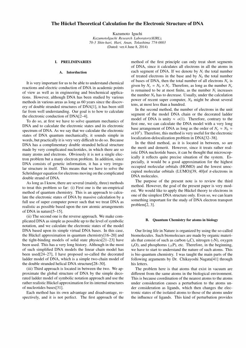
We consider first the simplest case, which is benzene. Ifcarbon atom is isolated, then there are four bonds around theatom where each bond consists of one valence electron. Butonce carbon meets other carbons such as in benzene, the co-ordination of atom is changed to the sp2-hybrid orbital; it isthree-coordination number plus one π-orbital perpendicular tothe plane of benzene.

Thus, in benzene there are six sp2-hybrid orbitals whichare triangular. They form the main hexagonal geometry ofbenzene. These bonds are called the σ-bonds through thesp2-hybrid orbitals. And there are still left six π-orbitals.These form the π-bonds between carbon atoms through theπ-orbitals, which are schematically represented by doublebonds.

Since three of four valence electrons in carbon are con-sumed to form the sp2-hybrid bonds, only one valence elec-tron left in carbon can exists for the π-electron. That is shownin Figure 2 as dot(•) near the carbon C.

FIG. 1. The electron configurations for C, N, O and P, respectively.(A) The electronic state of a carbon with three bonds. (B) The elec-tronic state of a carbon with two bonds. (C) The electronic state ofa nitrogen with three bonds. (D) The electronic state of a nitrogenwith two bonds. (E) The electronic state of an oxygen with a doublebond. (F) The electronic state of an oxygen with two bonds. (G) Theelectronic state of a phosphorus with four bonds. Here dots (•) meanelectrons, where electrons that occupy the π-orbitals are called theπ-electrons.

FIG. 2. The π-electron configuration in benzene molecule. The leftmost figure is a schematic diagram of benzene molecule. C is notconventionally shown at the carbon atom sites as in the middle figure.Using the previous electron configuration for carbon atom, there isone π-electron at each carbon atom. Here dots (•) mean π-electrons.

2. π-Electronic configurations in the A, G, C, T base molecules

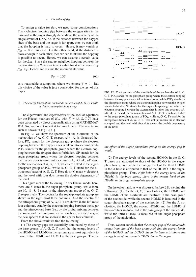
Let us consider the electronic configurations in the nitroge-nous base molecules such as adenine (A), guanine (G), cyto-sine (C) and thymine (T). The nitrogenous base molecules inDNA are classified into two types: purine and pyrimidine[42].A and G belong to purines, while C and T to prymidines,respectively. We may simply call the nitrogenous bases thebases, if there is no confusion. The molecular structures of A,G, C, T base molecules using the bond model are schemati-cally shown in Fig.3.

In the A molecule, there are five nitrogen N atoms, five car-

4

FIG. 3. The electron configurations for the bases of A, G, C and T,where there are 12 π-electrons and 10 π-orbitals in the A molecule;14 π-electrons and 11 π-orbitals in the G molecule; 10 π-electronsand 8 π-orbitals in the C molecule; and 10 π-electrons and 8 π-orbitals in the T molecule, respectively. Here dots (•) mean π-electrons.

bon C atoms and four hydrogen H atoms. In the G molecule,there are five nitrogen N atoms, five carbon C atoms, five hy-drogen H atoms and one oxygen O atom. In the C molecule,there are five hydrogen H atoms, four carbon C atoms, threenitrogen N atoms and one oxygen O atom. In the T molecule,there are six hydrogen H atoms, five carbon C atoms, two ni-trogen N atoms and two oxygen O atoms. Let us denote by|N|, |C| and |O| the total numbers of N, C and O atoms in thebase molecules.

Let us next consider the electron configurations in the π-orbitals of the nitrogenous bases of A, G, C and T. Here wecall such electrons in the π-orbitals π-electrons for the sakeof simplicity. In this paper we are concerned with only theπ-electrons and the π-orbitals in the system.

Applying the above basic knowledge of the quantum chem-istry to the biomolecules of nitrogenous bases, we find thefollowing: There are 12 π-electrons and 10 π-orbitals in the Amolecule; 14 π-electrons and 11 π-orbitals in the G molecule;10 π-electrons and 8 π-orbitals in the C molecule; and 10 π-electrons and 8 π-orbitals in the T molecule, respectively. Thisis summarized in Fig.3. Here we note that the carbon atom ofCH3 in the T molecule does not have any π-electron since itforms the sp3-hybrid orbitals. This provides 8 π-electrons forthe T molecule. Thus, we can summarize the above as in Table1.

TABLE I. The total numbers |N|, |C| and |O| of N, C and O atomsand of π-orbitals and π-electrons in the bases of A, G, C and T, re-spectively. Here there are 12 π-electrons and 10 π-orbitals in the Amolecule; 14 π-electrons and 11 π-orbitals in the G molecule; 10 π-electrons and 8 π-orbitals in the C molecule; and 10 π-electrons and8 π-orbitals in the T molecule, respectively.

Base A G C T|N| 5 5 3 5|C| 5 5 4 2|O| 0 1 1 2

Total 10 11 8 9π-orbitals 10 11 8 8π-electrons 12 14 10 10

3. Electronic configurations in molecules of sugar, phosphate andtriphosphate

Let us consider the electronic configurations in the sugar,the phosphate, the triphosphate, the sugar-phosphate and thesugar-triphosphate molecules[42], for later purposes[43–45].

To study the electronic states in such molecules was anold problem. As early as in 1960’s, by using the Huckeltheory[16–20], the quantum chemists[43–45] studied the elec-tronic properties of the complex molecules such as adeno-sine diphosphate (ADP) and adenosine triphosphate (ATP), inwhich the sugar is a ribose.

Naively saying, the Huckel theory can be applied to onlythe systems with a plane geometry such as benzene and ni-trogenous bases such as A, G, C, T[39, 46]. And also itis applicable to the systems with a linear geometry such aspolyacetylene[47, 48], where the π-orbitals are the nearestneighbor orbitals to each other so that there exists the overlapbetween the adjacent π-orbitals. So, the system with a tetra-hedral geometry such as the phosphate (−PO4) may not be agood system when we use the Huckel theory for π-orbitals,since the overlap between the π-orbitals is smaller than thatin the planer molecule systems. And by the same reason, thesystem of a sugar is not a good system for applying the Huckeltheory to it, since the π-orbitals at oxygen sites in the sugar arequite far from each other. Therefore, as the first approximationthe chemists in the 1960’s ignored the role of the π-orbitals inthe sugar molecule and treated only the π-orbitals at the phos-phate sites[49, 50]. Later, this point was improved to includethe role of the π-orbitals in the sugar molecule as well as thephosphate sites[51].

As was considered by Fukui et. al.[49, 50], the orbital mix-ing (hybridization) between the sp3-hybrid and the d-orbitalof the phosphorus should be taken into account, since there arefive valence electrons in the phosphorus so that four electronsoccupy the sp3-hybrid around the phosphorus atom and oneelectron occupies the orbital at the phosphorus atom. There-fore, one good approximation for treating the orbitals of thephosphorus is that we put five orbitals for five electrons sothat there are four orbitals forming the sp3-hybrid and one or-bital at the phosphorus site where each orbital can be occupied

5

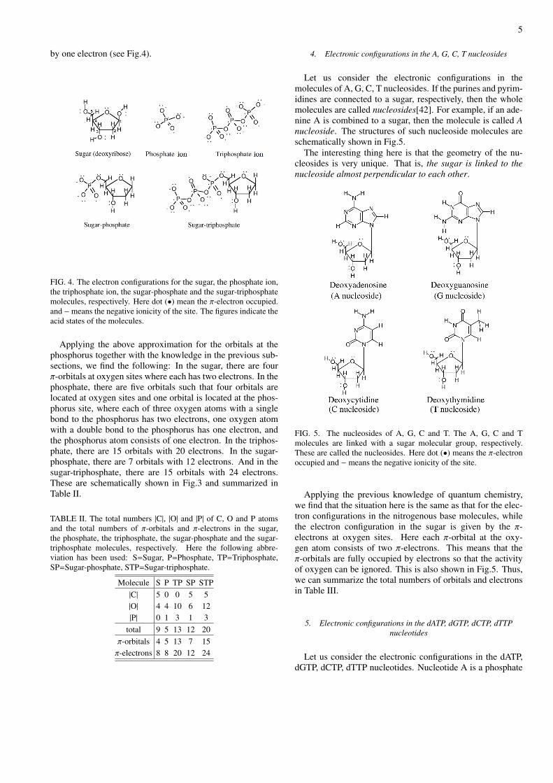
by one electron (see Fig.4).

FIG. 4. The electron configurations for the sugar, the phosphate ion,the triphosphate ion, the sugar-phosphate and the sugar-triphosphatemolecules, respectively. Here dot (•) mean the π-electron occupied.and −means the negative ionicity of the site. The figures indicate theacid states of the molecules.

Applying the above approximation for the orbitals at thephosphorus together with the knowledge in the previous sub-sections, we find the following: In the sugar, there are fourπ-orbitals at oxygen sites where each has two electrons. In thephosphate, there are five orbitals such that four orbitals arelocated at oxygen sites and one orbital is located at the phos-phorus site, where each of three oxygen atoms with a singlebond to the phosphorus has two electrons, one oxygen atomwith a double bond to the phosphorus has one electron, andthe phosphorus atom consists of one electron. In the triphos-phate, there are 15 orbitals with 20 electrons. In the sugar-phosphate, there are 7 orbitals with 12 electrons. And in thesugar-triphosphate, there are 15 orbitals with 24 electrons.These are schematically shown in Fig.3 and summarized inTable II.

TABLE II. The total numbers |C|, |O| and |P| of C, O and P atomsand the total numbers of π-orbitals and π-electrons in the sugar,the phosphate, the triphosphate, the sugar-phosphate and the sugar-triphosphate molecules, respectively. Here the following abbre-viation has been used: S=Sugar, P=Phosphate, TP=Triphosphate,SP=Sugar-phosphate, STP=Sugar-triphosphate.

Molecule S P TP SP STP|C| 5 0 0 5 5|O| 4 4 10 6 12|P| 0 1 3 1 3

total 9 5 13 12 20π-orbitals 4 5 13 7 15π-electrons 8 8 20 12 24

4. Electronic configurations in the A, G, C, T nucleosides

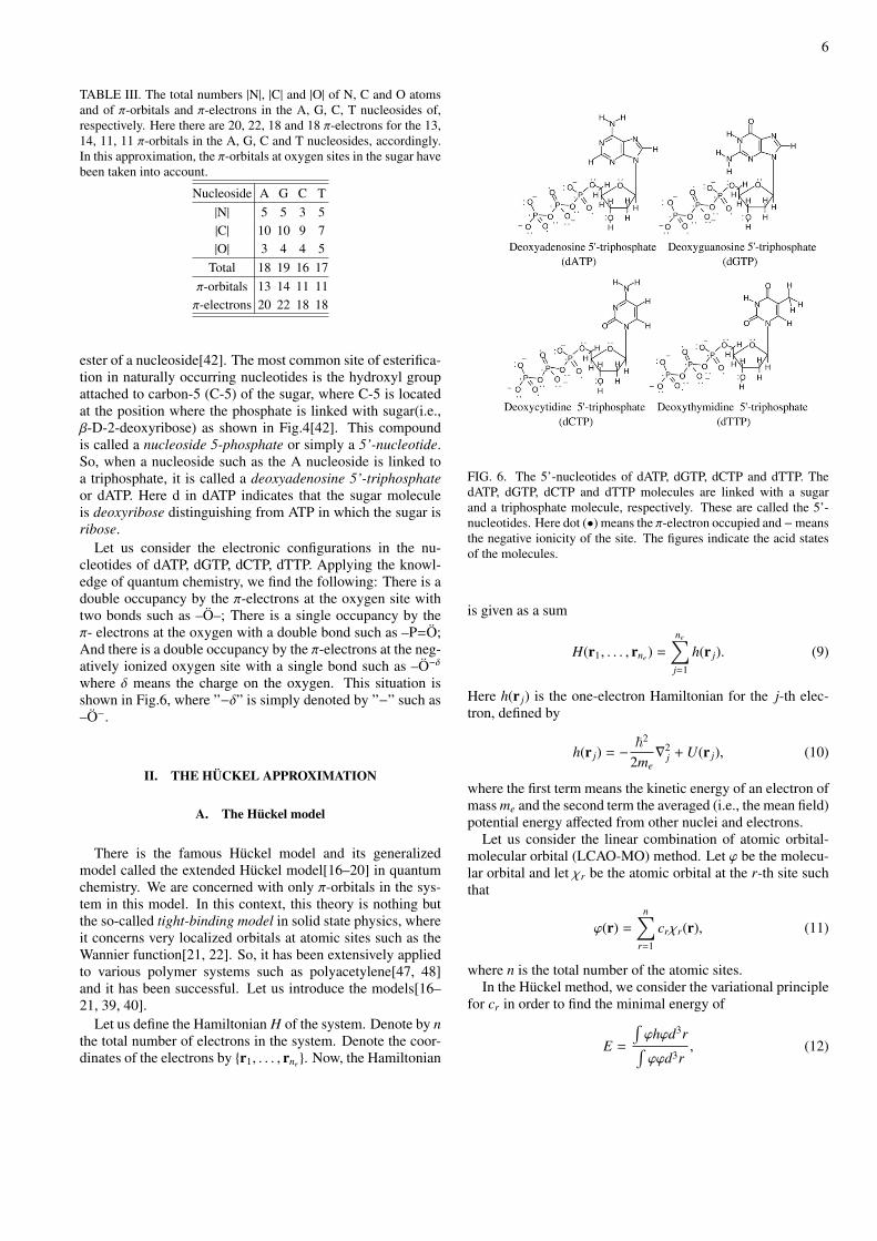
Let us consider the electronic configurations in themolecules of A, G, C, T nucleosides. If the purines and pyrim-idines are connected to a sugar, respectively, then the wholemolecules are called nucleosides[42]. For example, if an ade-nine A is combined to a sugar, then the molecule is called Anucleoside. The structures of such nucleoside molecules areschematically shown in Fig.5.

The interesting thing here is that the geometry of the nu-cleosides is very unique. That is, the sugar is linked to thenucleoside almost perpendicular to each other.

FIG. 5. The nucleosides of A, G, C and T. The A, G, C and Tmolecules are linked with a sugar molecular group, respectively.These are called the nucleosides. Here dot (•) means the π-electronoccupied and − means the negative ionicity of the site.

Applying the previous knowledge of quantum chemistry,we find that the situation here is the same as that for the elec-tron configurations in the nitrogenous base molecules, whilethe electron configuration in the sugar is given by the π-electrons at oxygen sites. Here each π-orbital at the oxy-gen atom consists of two π-electrons. This means that theπ-orbitals are fully occupied by electrons so that the activityof oxygen can be ignored. This is also shown in Fig.5. Thus,we can summarize the total numbers of orbitals and electronsin Table III.

5. Electronic configurations in the dATP, dGTP, dCTP, dTTPnucleotides

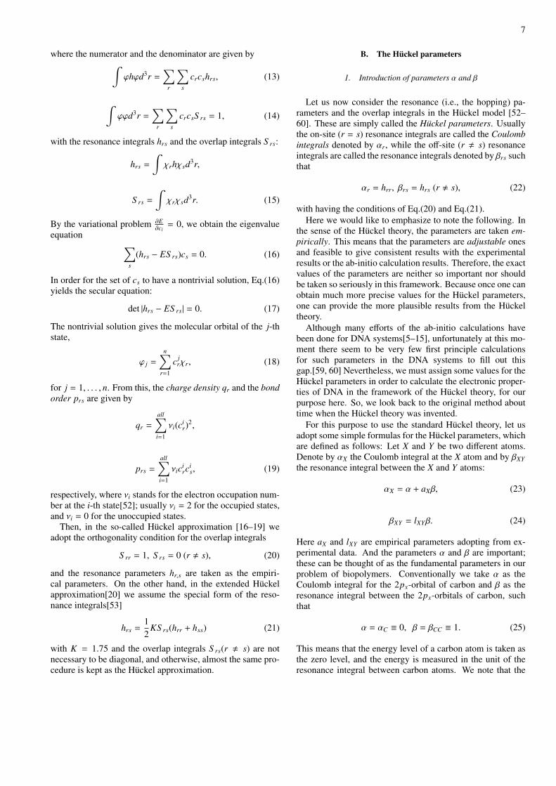
Let us consider the electronic configurations in the dATP,dGTP, dCTP, dTTP nucleotides. Nucleotide A is a phosphate

6

TABLE III. The total numbers |N|, |C| and |O| of N, C and O atomsand of π-orbitals and π-electrons in the A, G, C, T nucleosides of,respectively. Here there are 20, 22, 18 and 18 π-electrons for the 13,14, 11, 11 π-orbitals in the A, G, C and T nucleosides, accordingly.In this approximation, the π-orbitals at oxygen sites in the sugar havebeen taken into account.

Nucleoside A G C T|N| 5 5 3 5|C| 10 10 9 7|O| 3 4 4 5

Total 18 19 16 17π-orbitals 13 14 11 11π-electrons 20 22 18 18

ester of a nucleoside[42]. The most common site of esterifica-tion in naturally occurring nucleotides is the hydroxyl groupattached to carbon-5 (C-5) of the sugar, where C-5 is locatedat the position where the phosphate is linked with sugar(i.e.,β-D-2-deoxyribose) as shown in Fig.4[42]. This compoundis called a nucleoside 5-phosphate or simply a 5’-nucleotide.So, when a nucleoside such as the A nucleoside is linked toa triphosphate, it is called a deoxyadenosine 5’-triphosphateor dATP. Here d in dATP indicates that the sugar moleculeis deoxyribose distinguishing from ATP in which the sugar isribose.

Let us consider the electronic configurations in the nu-cleotides of dATP, dGTP, dCTP, dTTP. Applying the knowl-edge of quantum chemistry, we find the following: There is adouble occupancy by the π-electrons at the oxygen site withtwo bonds such as –O–; There is a single occupancy by theπ- electrons at the oxygen with a double bond such as –P=O;And there is a double occupancy by the π-electrons at the neg-atively ionized oxygen site with a single bond such as –O−δ

where δ means the charge on the oxygen. This situation isshown in Fig.6, where ”−δ” is simply denoted by ”−” such as–O−.

II. THE HUCKEL APPROXIMATION

A. The Huckel model

There is the famous Huckel model and its generalizedmodel called the extended Huckel model[16–20] in quantumchemistry. We are concerned with only π-orbitals in the sys-tem in this model. In this context, this theory is nothing butthe so-called tight-binding model in solid state physics, whereit concerns very localized orbitals at atomic sites such as theWannier function[21, 22]. So, it has been extensively appliedto various polymer systems such as polyacetylene[47, 48]and it has been successful. Let us introduce the models[16–21, 39, 40].

Let us define the Hamiltonian H of the system. Denote by nthe total number of electrons in the system. Denote the coor-dinates of the electrons by {r1, . . . , rne }. Now, the Hamiltonian

FIG. 6. The 5’-nucleotides of dATP, dGTP, dCTP and dTTP. ThedATP, dGTP, dCTP and dTTP molecules are linked with a sugarand a triphosphate molecule, respectively. These are called the 5’-nucleotides. Here dot (•) means the π-electron occupied and −meansthe negative ionicity of the site. The figures indicate the acid statesof the molecules.

is given as a sum

H(r1, . . . , rne ) =ne∑j=1

h(r j). (9)

Here h(r j) is the one-electron Hamiltonian for the j-th elec-tron, defined by

h(r j) = −ℏ2

2me∇2

j + U(r j), (10)

where the first term means the kinetic energy of an electron ofmass me and the second term the averaged (i.e., the mean field)potential energy affected from other nuclei and electrons.

Let us consider the linear combination of atomic orbital-molecular orbital (LCAO-MO) method. Let φ be the molecu-lar orbital and let χr be the atomic orbital at the r-th site suchthat

φ(r) =n∑

r=1

crχr(r), (11)

where n is the total number of the atomic sites.In the Huckel method, we consider the variational principle

for cr in order to find the minimal energy of

E =

∫φhφd3r∫φφd3r

, (12)

7

where the numerator and the denominator are given by∫φhφd3r =

∑r

∑s

crcshrs, (13)

∫φφd3r =

∑r

∑s

crcsS rs = 1, (14)

with the resonance integrals hrs and the overlap integrals S rs:

hrs =

∫χrhχsd3r,

S rs =

∫χrχsd3r. (15)

By the variational problem ∂E∂cl= 0, we obtain the eigenvalue

equation ∑s

(hrs − ES rs)cs = 0. (16)

In order for the set of cs to have a nontrivial solution, Eq.(16)yields the secular equation:

det |hrs − ES rs| = 0. (17)

The nontrivial solution gives the molecular orbital of the j-thstate,

φ j =

n∑r=1

c jrχr, (18)

for j = 1, . . . , n. From this, the charge density qr and the bondorder prs are given by

qr =

all∑i=1

νi(cir)

2,

prs =

all∑i=1

νicirc

is, (19)

respectively, where νi stands for the electron occupation num-ber at the i-th state[52]; usually νi = 2 for the occupied states,and νi = 0 for the unoccupied states.

Then, in the so-called Huckel approximation [16–19] weadopt the orthogonality condition for the overlap integrals

S rr = 1, S rs = 0 (r , s), (20)

and the resonance parameters hr,s are taken as the empiri-cal parameters. On the other hand, in the extended Huckelapproximation[20] we assume the special form of the reso-nance integrals[53]

hrs =12

KS rs(hrr + hss) (21)

with K = 1.75 and the overlap integrals S rs(r , s) are notnecessary to be diagonal, and otherwise, almost the same pro-cedure is kept as the Huckel approximation.

B. The Huckel parameters

1. Introduction of parameters α and β

Let us now consider the resonance (i.e., the hopping) pa-rameters and the overlap integrals in the Huckel model [52–60]. These are simply called the Huckel parameters. Usuallythe on-site (r = s) resonance integrals are called the Coulombintegrals denoted by αr, while the off-site (r , s) resonanceintegrals are called the resonance integrals denoted by βrs suchthat

αr = hrr, βrs = hrs (r , s), (22)

with having the conditions of Eq.(20) and Eq.(21).Here we would like to emphasize to note the following. In

the sense of the Huckel theory, the parameters are taken em-pirically. This means that the parameters are adjustable onesand feasible to give consistent results with the experimentalresults or the ab-initio calculation results. Therefore, the exactvalues of the parameters are neither so important nor shouldbe taken so seriously in this framework. Because once one canobtain much more precise values for the Huckel parameters,one can provide the more plausible results from the Huckeltheory.

Although many efforts of the ab-initio calculations havebeen done for DNA systems[5–15], unfortunately at this mo-ment there seem to be very few first principle calculationsfor such parameters in the DNA systems to fill out thisgap.[59, 60] Nevertheless, we must assign some values for theHuckel parameters in order to calculate the electronic proper-ties of DNA in the framework of the Huckel theory, for ourpurpose here. So, we look back to the original method abouttime when the Huckel theory was invented.

For this purpose to use the standard Huckel theory, let usadopt some simple formulas for the Huckel parameters, whichare defined as follows: Let X and Y be two different atoms.Denote by αX the Coulomb integral at the X atom and by βXYthe resonance integral between the X and Y atoms:

αX = α + aXβ, (23)

βXY = lXYβ. (24)

Here aX and lXY are empirical parameters adopting from ex-perimental data. And the parameters α and β are important;these can be thought of as the fundamental parameters in ourproblem of biopolymers. Conventionally we take α as theCoulomb integral for the 2px-orbital of carbon and β as theresonance integral between the 2px-orbitals of carbon, suchthat

α = αC ≡ 0, β = βCC ≡ 1. (25)

This means that the energy level of a carbon atom is taken asthe zero level, and the energy is measured in the unit of theresonance integral between carbon atoms. We note that the

8

empirical values obtained from experiments are usually givenby[43–45]

α ≈ −6.30 ∼ −6.61eV, β ≈ −2.93 ∼ −2.95eV. (26)

There are some examples for the parameters of αX and βXY .They are summarized in Table 4 and Table 5, respectively.

TABLE IV. The empirical parameters of the Coulomb integral pa-rameters αX of atom X in the unit of eV . For an example, we adoptthe values from Ref.[43–45]. Here αC = α = −6.61eV (which willbe regarded as the zero energy level such that αC = α = 0) andαP = α − β = −3.66eV has been assumed with β = −2.95ev.

Atom, X C O N PαX −6.61 −8.73 −10.94 −3.66

TABLE V. The empirical parameters of the resonance integrals βXY

between X and Y atoms in the unit of β. For an example, we adoptthe values from Ref.[43–45].

Atoms, XY CC OC CN OPβXY 1 2 1 ≈ 1

2. Convienient formulas for the Huckel parameters

The above values of the Huckel parameters α and β are es-sentially those for the empty site without electrons. When π-electrons occupy an atomic site, there are a few good formulasfor calculating the numerical values of α and β.

Denote by αX the Coulomb integral of the atomic site Xwithout any electron. Denote by αX the Coulomb integral ofthe atomic site X with one electron occupied. And denoteby αX the Coulomb integral of the atomic site X with twoelectrons occupied.

The Sandorfy’s formulaWe now have

αX =χX

χCα = α +

χX − χC

χC· 4.1β, (27)

where χX (χC) means the Pauling’s electronegativity of X(carbon) atom[58]. Since this method was proposed bySandorfy[54], this is called the Sandorfy’s formula in quan-tum chemistry[44, 45].

The Streitwieser’s formulaTo use the Sandorfy’s formula for αX , Streitwieser[55] intro-duced the following formula:

αX � αX + β. (28)

This is called the Streitwieser’s formula in quantumchemistry[44, 45].

The Mulliken’s formulaOn the other hand, there are a couple of methods to evaluate

lXY in Eq.(24). One method was proposed by Mulliken[56, 57]such that

lCX =S CX

S CC, (29)

where S CX stands for the overlap integral between carbon andX atoms and S CC the overlap integral between carbon atomswith assuming S CC = 0.25. Another method uses the formula:

lCX =

(1.397RCX

)4

, (30)

where RCX is the inter-distance between the C and Xatoms[44, 45].

These formulas are just empirical ones, which should beable to be derived by the ab-initio method using a supercom-putor. However, unless one can use such a super high per-formance computer system, one can obtain some appropriatevalues for the Huckel parameters below. This is the advan-tage of the above formulas such that before we have to use thehighly expensive tools we can estimate what the values areprobable to be obtained.

3. The Huckel parameters for biomolecules

For our purpose that we apply the Huckel model tobiomolecules of DNA, we have to set up the numerical val-ues of the Huckel parameters. Since the biomolecules consistof the atoms C, N, O, P, let us find the plausible values of theHuckel parameters for them.

The Pauling’s electronegativity[58] for carbon (C), nitrogen(N), oxygen (O) and phosphorus (P) are given as follows:

χC ≈ 2.55, χN ≈ 3.0, χO ≈ 3.5, χP ≈ 2.1. (31)

Remembering our definition of the Huckel parameters for car-bon [see Eq.(25)] and using the Sandorfy’s formula[54] [seeEq.(27)], we find

αC = αC = α,

αN = α +χN − χC

χC· 4.1β = α + 0.723β,

αO = α +χO − χC

χC· 4.1β = α + 1.53β,

αP = α +χP − χC

χC· 4.1β = α − 0.724β, (32)

Using next the Streitwieser’s formula[55] [see Eq.(28)], weobtain

αO = αO + β = α + 2.53β,

αN = αN + β = α + 1.72β. (33)

9

And using the Mulliken’s formula[56] [see Eq.(29)], we esti-mate the approximated values as

βC−C = β, βC=C = 1.1β,

βC−N = βC−N = 0.8β, βC=N = 1.1β,

βC=O = 1.7β. (34)

For example, the above value of βC−C is obtained as follows:Substituting the distance between C-C bond RC−C = 1.379Åinto Eq.(30), we obtain lC−C = 1. Hence, βC−C = β. Simi-larly for βC=N , we take RC=N = 1.37Å and substitute it intoEq.(30). We obtain βC=N = 1.1β. For βC=C , we have takenapproximately the same value as βC=N .

We note here that we will use the above parametersthroughout this paper. The adoption of these phenomenolog-ical values is just a convention for our purpose here. And ifone can get the more accurate values from the ab-initio cal-culations, then we can always replace them by the new set ofvalues.[59, 60]

C. Electronic states of benzene C6H6

Before going to consider the electronic states ofbiomolecules, let us consider one of the simplest case ofbenzene(Fig.2)[40]. From this simple example we can learnwhat will happen to and how we can solve the problem[43–45].

1. The Huckel matrix for benzene C6H6

Let us find the Huckel matrix for benzene, C6H6. In thecase of benzene, the resonance parameters are given by onlyαC = αC = α = 0 and βC−C = βC=C = β = 1 for simplicity.Numbering the sites of π-orbitals from 1 to 6, then we obtainthe following Huckel matrix:

HC6H6 =

α β 0 0 0 ββ α β 0 0 00 β α β 0 00 0 β α β 00 0 0 β α ββ 0 0 0 β α

. (35)

2. The eigenequation for benzene C6H6

Defining the wavefunction φ =∑6

r=1 crχr[see Eq.(11)], andfrom Eq.(16) together with the Huckel matrix for benzeneC6H6, we obtain the eigenequation:

(HC6H6 − E16)c =

α − E β 0 0 0 β

β α − E β 0 0 00 β α − E β 0 00 0 β α − E β 00 0 0 β α − E β

β 0 0 0 β α − E

c1

c2

c3

c4

c5

c6

= 0, (36)

where cr (r = 1, · · · , 6) in the vector c is the wave function forthe r-th π-orbital at r-th carbon site, and E the energy of thesix π-electrons.

3. The eigenvalues of the Huckel matrix for benzene C6H6

Digonalizing the eigenequation:

det |HC6H6 − E16| =

∣∣∣∣∣∣∣∣∣∣∣∣∣∣∣∣∣∣∣

α − E β 0 0 0 β

β α − E β 0 0 00 β α − E β 0 00 0 β α − E β 00 0 0 β α − E β

β 0 0 0 β α − E

∣∣∣∣∣∣∣∣∣∣∣∣∣∣∣∣∣∣∣= 0, (37)

we find the six eigenvalues E j and the corresponding sixeigenfunctions φ j. The result is very simple since there issymmetry in the molecule of benzene C6H6.

Solving Eq.(36) and Eq.(37), we obtain the following equa-tion for c j

s:

c jr =

√1n

ei 2π jn r, (38)

where j = 1, · · · , n and we set n = 6 for benzene C6H6. Thisdescribes the wave function at site r with the j-th state of en-ergy level E j:

E j = α + 2β cos(

2π jn

), (39)

with the corresponding the j-th state being given by

φ j =

√1n

n∑r=1

ei 2π jn rχr. (40)

III. ELECTRONIC STATES OF NUCLEOTIDES

A. Electronic states of single bases of A, G, C and T

In this section, we are going to study the electronic statesof the single nitrogenous bases of A, G, C and T, in terms ofthe language of the Huckel theory[16–20], respectively.

To do so, (i) we first specify the molecule so that we canrepresent the matrix of the Huckel model (we will call the

10

matrix the Huckel matrix) in terms of the Huckel parameters,αX and βXY for the molecule.

(ii) Second, thanks to MATHEMATICA, we use it to solvedirectly the secular equation represented by the Huckel matrixin order to obtain its eigenstates and eigenvalues.

(iii) Third, we count the π-electrons and put them in theenergy levels in order to know the HOMO and LUMO statesof the system.

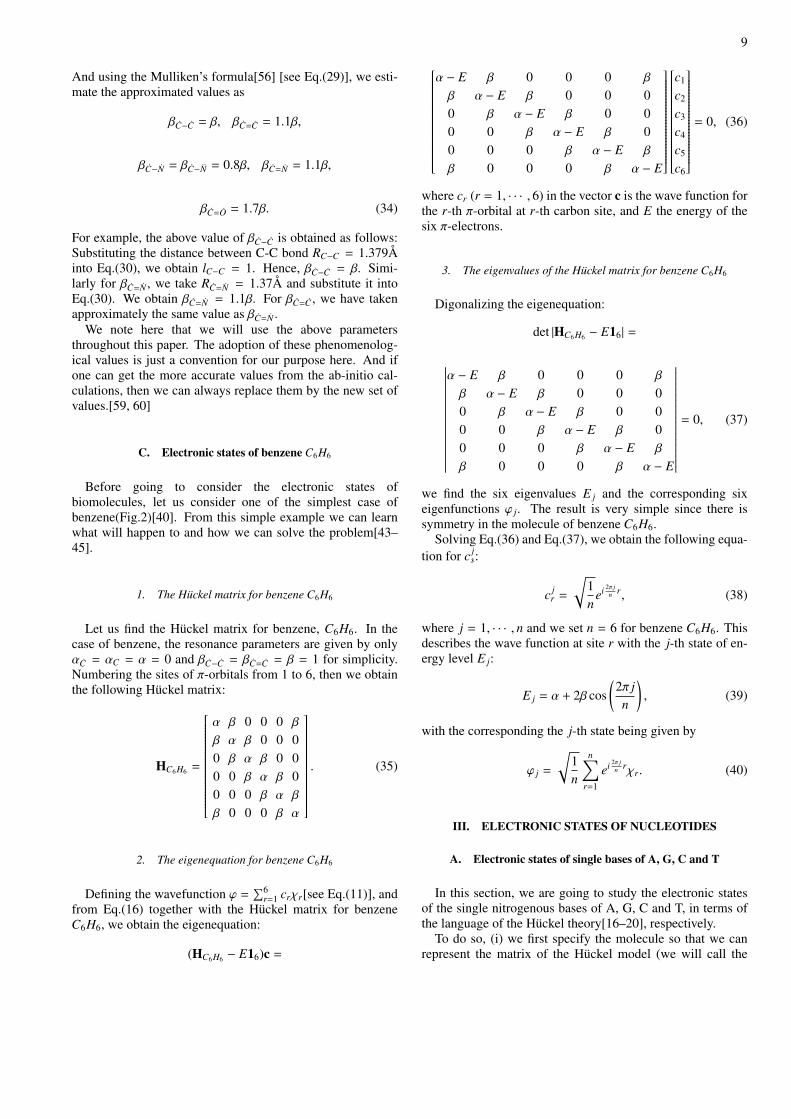
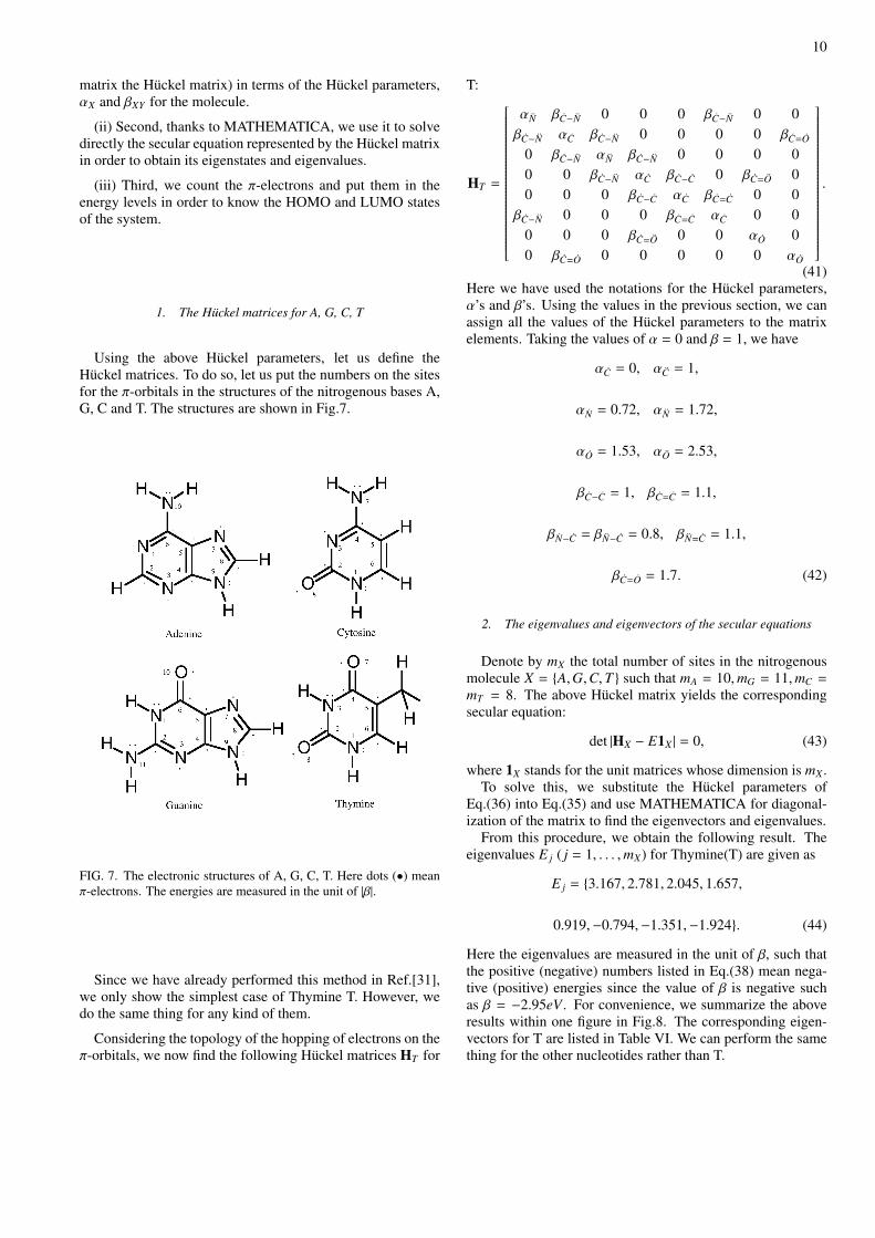
1. The Huckel matrices for A, G, C, T

Using the above Huckel parameters, let us define theHuckel matrices. To do so, let us put the numbers on the sitesfor the π-orbitals in the structures of the nitrogenous bases A,G, C and T. The structures are shown in Fig.7.

FIG. 7. The electronic structures of A, G, C, T. Here dots (•) meanπ-electrons. The energies are measured in the unit of |β|.

Since we have already performed this method in Ref.[31],we only show the simplest case of Thymine T. However, wedo the same thing for any kind of them.

Considering the topology of the hopping of electrons on theπ-orbitals, we now find the following Huckel matrices HT for

T:

HT =

αN βC−N 0 0 0 βC−N 0 0βC−N αC βC−N 0 0 0 0 βC=O

0 βC−N αN βC−N 0 0 0 00 0 βC−N αC βC−C 0 βC=O 00 0 0 βC−C αC βC=C 0 0βC−N 0 0 0 βC=C αC 0 0

0 0 0 βC=O 0 0 αO 00 βC=O 0 0 0 0 0 αO

.

(41)Here we have used the notations for the Huckel parameters,α’s and β’s. Using the values in the previous section, we canassign all the values of the Huckel parameters to the matrixelements. Taking the values of α = 0 and β = 1, we have

αC = 0, αC = 1,

αN = 0.72, αN = 1.72,

αO = 1.53, αO = 2.53,

βC−C = 1, βC=C = 1.1,

βN−C = βN−C = 0.8, βN=C = 1.1,

βC=O = 1.7. (42)

2. The eigenvalues and eigenvectors of the secular equations

Denote by mX the total number of sites in the nitrogenousmolecule X = {A,G,C,T } such that mA = 10,mG = 11,mC =

mT = 8. The above Huckel matrix yields the correspondingsecular equation:

det |HX − E1X | = 0, (43)

where 1X stands for the unit matrices whose dimension is mX .To solve this, we substitute the Huckel parameters of

Eq.(36) into Eq.(35) and use MATHEMATICA for diagonal-ization of the matrix to find the eigenvectors and eigenvalues.

From this procedure, we obtain the following result. Theeigenvalues E j ( j = 1, . . . ,mX) for Thymine(T) are given as

E j = {3.167, 2.781, 2.045, 1.657,

0.919,−0.794,−1.351,−1.924}. (44)

Here the eigenvalues are measured in the unit of β, such thatthe positive (negative) numbers listed in Eq.(38) mean nega-tive (positive) energies since the value of β is negative suchas β = −2.95eV . For convenience, we summarize the aboveresults within one figure in Fig.8. The corresponding eigen-vectors for T are listed in Table VI. We can perform the samething for the other nucleotides rather than T.

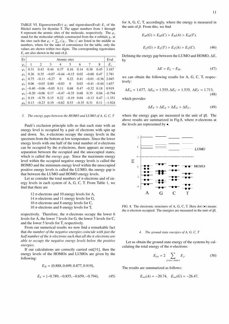
11

TABLE VI. Eigenvectors(Ev) φ j and eigenvalues(Eval) E j of theHuckel matrix for thymine T. The upper numbers from 1 through8 represent the atomic sites of the molecule, respectively. The φ j

stand for the molecular orbitals constructed from the π-orbitals χr atthe sites such that φ j =

∑n c j

rχr. The c jr are listed in the middle as

numbers, where for the sake of convenience for the table, only thevalues are shown within two digits. The corresponding eigenvaluesE j are also shown in the unit of β.

Ev Atomic sites Evalφ j 1 2 3 4 5 6 7 8 E j

φ1 0.31 0.43 0.44 0.37 0.16 0.14 0.38 0.45 3.167φ2 0.26 0.35 −0.07 −0.44 −0.15 0.02 −0.60 0.47 2.781φ3 0.75 −0.11 −0.27 0 0.22 0.41 −0.01 −0.36 2.045φ4 0.06 −0.03 0.80 −0.03 0 0.03 −0.41 −0.44 1.657φ5 −0.40 −0.06 −0.05 0.11 0.68 0.47 −0.32 0.18 0.919φ6 −0.20 −0.06 0.17 −0.47 −0.35 0.68 0.35 0.04 −0.794φ7 0.19 −0.79 0.15 0.22 −0.19 0.04 −0.13 0.47 −1.351φ8 0.13 −0.23 0.19 −0.62 0.53 −0.35 0.31 0.11 −1.924

3. The energy gaps between the HOMO and LUMO of A, G, C, T

Pauli’s exclusion principle tells us that each state with anenergy level is occupied by a pair of electrons with spin upand down. So, π-electrons occupy the energy levels in thespectrum from the bottom at low temperature. Since the lowerenergy levels with one half of the total number of π-electronscan be occupied by the π-electrons, there appears an energyseparation between the occupied and the unoccupied states,which is called the energy gap. Since the maximum energylevel within the occupied negative energy levels is called theHOMO and the minimum energy level within the unoccupiedpositive energy levels is called the LUMO, the energy gap isthat between the LUMO and HOMO energy levels.

Let us consider the total numbers of π-electrons and of en-ergy levels in each system of A, G, C, T. From Table 1, wefind that there are

12 π-electrons and 10 energy levels for A,14 π-electrons and 11 energy levels for G,10 π-electrons and 8 energy levels for C,10 π-electrons and 8 energy levels for T,

respectively. Therefore, the π-electrons occupy the lower 6levels for A, the lower 7 levels for G, the lower 5 levels for C,and the lower 5 levels for T, respectively.

From our numerical results we now find a remarkable factthat the number of the negative energies coincide with just thehalf number of the π-electrons such that all the π-electrons areable to occupy the negative energy levels below the positiveenergies.

If our calculations are correctly carried out[31], then theenergy levels of the HOMOs and LUMOs are given by thefollowing:

EH = {0.888, 0.699, 0.877, 0.919},

EL = {−0.789,−0.855,−0.659,−0.794}, (45)

for A, G, C, T, accordingly, where the energy is measured inthe unit of β. From this, we find

EH(G) > EH(C) > EH(A) > EH(T ),

EL(G) > EL(T ) > EL(A) > EL(C). (46)

Defining the energy gap between the LUMO and HOMO, ∆E,by

∆E = EL − EH , (47)

we can obtain the following results for A, G, C, T, respec-tively:

∆EA = 1.677, ∆EG = 1.555,∆EC = 1.535, ∆ET = 1.713,(48)

which provides

∆ET > ∆EA > ∆EG > ∆EC , (49)

where the energy gaps are measured in the unit of |β|. Theabove results are summarized in Fig.8, where π-electrons atthe levels are represented by •.

FIG. 8. The electronic structures of A, G, C, T. Here dot (•) meansthe π-electron occupied. The energies are measured in the unit of |β|.

4. The ground state energies of A, G, C, T

Let us obtain the ground state energy of the systems by cal-culating the total energy of the π-electrons:

Etot = 2∑

j=occ.states

E j. (50)

The results are summarized as follows:

Etot(A) = −20.74, Etot(G) = −26.47,

12

Etot(C) = −19.05, Etot(T ) = −21.14, (51)

which gives

Etot(C) > Etot(A) > Etot(T ) > Etot(G), (52)

where the energies are measured in the unit of |β|. This showsthat since the lower the ground state energy the more stable thesystem, the most stable molecule is G while the most unstablemolecule is C.

Finally we note that Eq.(40), Eq.(45) and Eq.(46) qual-itatively agree with the results in the early calculations ofLadik[25, 26] and in the recent ab-initio calculations [5–15].Therefore, even though our approach is phenomenological us-ing many empirical values for the Huckel parameters, the re-sults obtained are quite encouraging. This situation gives usa starting point as the zeroth approximation for the furtherstudy.

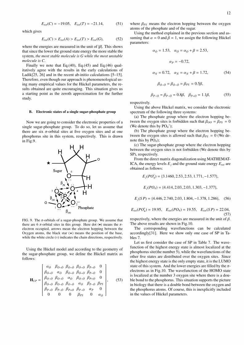
B. Electronic states of a single sugar-phosphate group

Now we are going to consider the electronic properties of asingle sugar-phosphate group. To do so, let us assume thatthere are six π-orbital sites at five oxygen sites and at onephosphorus site in this system, respectively. This is drawnin Fig.9.

FIG. 9. The π-orbitals of a sugar-phosphate group. We assume thatthere are 6 π-orbital sites in this group. Here dot (•) means the π-electron occupied, arrows mean the electron hopping between theOxygen atoms, the black star (⋆) means the position of the base,while the white circle (◦) indicates the chain directions, respectively.

Using the Huckel model and according to the geometry ofthe sugar-phosphate group, we define the Huckel matrix asfollows:

HS P =

αO βO−O βO−O βO−O βP−O 0βO−O αO βO−O βO−O βP−O 0βO−O βO−O αO βO−O βP=O 0βO−O βO−O βO−O αO βP−O βPS

βP−O βP−O βP=O βP−O αP 00 0 0 βPS 0 αO

, (53)

where βPS means the electron hopping between the oxygenatoms of the phosphate and of the sugar.

Using the method explained in the previous section and as-suming that α = 0 and β = 1, we assign the following Huckelparameters:

αO = 1.53, αO = αO + β = 2.53,

αP = −0.72,

αN = 0.72, αN = αN + β = 1.72, (54)

βO−O = βO−O = βPS = 0.5β,

βP−O = βP−O = 0.8β, βP=O = 1.1β, (55)

respectively.Using the above Huckel matrix, we consider the electronic

spectrum of the following three systems:(a) The phosphate group where the electron hopping be-

tween the oxygen sites is forbidden such that βOO = βPS = 0(We denote this by PO4’);

(b) The phosphate group where the electron hopping be-tween the oxygen sites is allowed such that βPS = 0 (We de-note this by PO4);

(c) The sugar-phosphate group where the electron hoppingbetween the oxygen sites is not forbidden (We denote this bySP), respectively.

From the direct matrix diagonalization using MATHEMAT-ICA, the energy levels E j and the ground state energy Etot areobtained as follows:

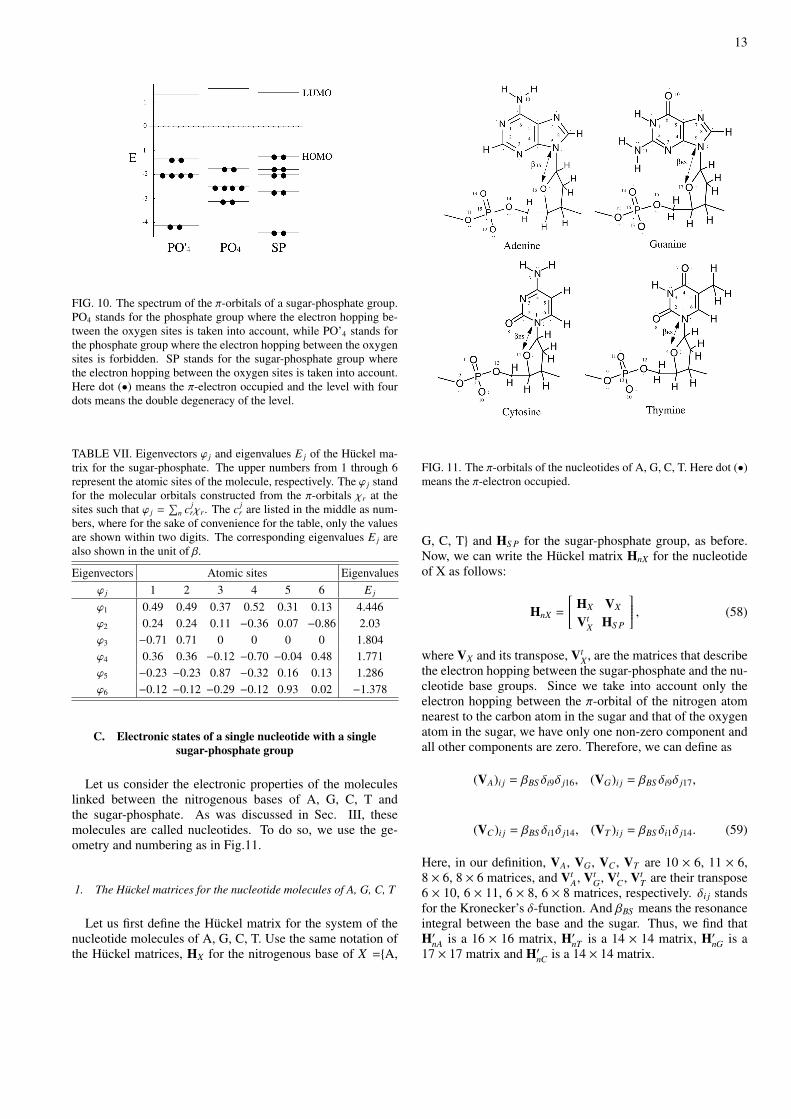
E j(PO′4) = {3.1460, 2.53, 2.53, 1.771,−1.577},

E j(PO4) = {4.414, 2.03, 2.03, 1.303,−1.377},

E j(S P) = {4.446, 2.740, 2.03, 1.804,−1.378, 1.286}, (56)

Etot(PO′4) = 19.95, Etot(PO4) = 19.55, Etot(S P) = 22.04,(57)

respectively, where the energies are measured in the unit of β.The above results are shown in Fig.10.

The corresponding wavefunctions can be calculatedaccordingly[31]. Here we show only one case of SP in Ta-bles 7.

Let us first consider the case of SP in Table 7. The wave-function of the highest energy state is almost localized at thephosphorus site(the number 5), while the wavefunctions of theother five states are distributed over the oxygen sites. Sincethe highest energy state is the only empty state, it is the LUMOstate of this system. And the lower energies are filled by the π-electrons as in Fig.10. The wavefunction of the HOMO stateis localized at the number 3 oxygen site where there is a dou-ble bond to the phosphorus. This situation supports the picturein biology that there is a double bond between the oxygen andthe phosphorus atoms. Of course, this is inexplicitly includedin the values of Huckel parameters.

13

FIG. 10. The spectrum of the π-orbitals of a sugar-phosphate group.PO4 stands for the phosphate group where the electron hopping be-tween the oxygen sites is taken into account, while PO’4 stands forthe phosphate group where the electron hopping between the oxygensites is forbidden. SP stands for the sugar-phosphate group wherethe electron hopping between the oxygen sites is taken into account.Here dot (•) means the π-electron occupied and the level with fourdots means the double degeneracy of the level.

TABLE VII. Eigenvectors φ j and eigenvalues E j of the Huckel ma-trix for the sugar-phosphate. The upper numbers from 1 through 6represent the atomic sites of the molecule, respectively. The φ j standfor the molecular orbitals constructed from the π-orbitals χr at thesites such that φ j =

∑n c j

rχr. The c jr are listed in the middle as num-

bers, where for the sake of convenience for the table, only the valuesare shown within two digits. The corresponding eigenvalues E j arealso shown in the unit of β.

Eigenvectors Atomic sites Eigenvaluesφ j 1 2 3 4 5 6 E j

φ1 0.49 0.49 0.37 0.52 0.31 0.13 4.446φ2 0.24 0.24 0.11 −0.36 0.07 −0.86 2.03φ3 −0.71 0.71 0 0 0 0 1.804φ4 0.36 0.36 −0.12 −0.70 −0.04 0.48 1.771φ5 −0.23 −0.23 0.87 −0.32 0.16 0.13 1.286φ6 −0.12 −0.12 −0.29 −0.12 0.93 0.02 −1.378

C. Electronic states of a single nucleotide with a singlesugar-phosphate group

Let us consider the electronic properties of the moleculeslinked between the nitrogenous bases of A, G, C, T andthe sugar-phosphate. As was discussed in Sec. III, thesemolecules are called nucleotides. To do so, we use the ge-ometry and numbering as in Fig.11.

1. The Huckel matrices for the nucleotide molecules of A, G, C, T

Let us first define the Huckel matrix for the system of thenucleotide molecules of A, G, C, T. Use the same notation ofthe Huckel matrices, HX for the nitrogenous base of X ={A,

FIG. 11. The π-orbitals of the nucleotides of A, G, C, T. Here dot (•)means the π-electron occupied.

G, C, T} and HS P for the sugar-phosphate group, as before.Now, we can write the Huckel matrix HnX for the nucleotideof X as follows:

HnX =

HX VX

VtX HS P

, (58)

where VX and its transpose, VtX , are the matrices that describe

the electron hopping between the sugar-phosphate and the nu-cleotide base groups. Since we take into account only theelectron hopping between the π-orbital of the nitrogen atomnearest to the carbon atom in the sugar and that of the oxygenatom in the sugar, we have only one non-zero component andall other components are zero. Therefore, we can define as

(VA)i j = βBS δi9δ j16, (VG)i j = βBS δi9δ j17,

(VC)i j = βBS δi1δ j14, (VT )i j = βBS δi1δ j14. (59)

Here, in our definition, VA, VG, VC , VT are 10 × 6, 11 × 6,8 × 6, 8 × 6 matrices, and Vt

A, VtG, Vt

C , VtT are their transpose

6 × 10, 6 × 11, 6 × 8, 6 × 8 matrices, respectively. δi j standsfor the Kronecker’s δ-function. And βBS means the resonanceintegral between the base and the sugar. Thus, we find thatH′nA is a 16 × 16 matrix, H′nT is a 14 × 14 matrix, H′nG is a17 × 17 matrix and H′nC is a 14 × 14 matrix.

14

2. The value of βBS

To assign a value for βBS , we need some considerations.The π-electron hopping βBS between the oxygen sites in thebase and in the sugar strongly depends on the geometry of thesingle strand of DNA. So, if the distance between the oxygensites of the base and the sugar is far apart, then we can thinkthat the hopping is hard to occur. Hence, it may vanish asβBS = 0 in this case. On the other hand, if the distance isclose enough to each other, then we can think that the hoppingis possible to occur. Hence, we can assume a certain valuefor the βBS . Since the nearest neighbor hopping between thecarbon atoms is β we can take a value for it in between 0 ≤βBS ≤ β. Hence, we assume the intermediate value

βBS = 0.5β (60)

as a reasonable assumption, where we choose β = 1. Butthis choice of the value is just a convention for the rest of thispaper.

3. The energy levels of the nucleotide molecules of A, G, C, T witha single sugar-phosphate group

The eigenvalues and eigenvectors of the secular equationsfor the Huckel matrices of HnX with X = {A,G,C,T } havebeen calculated by direct diagonalization using MATHEMAT-ICA. So, we do not repeat it too much here. The results aresuch as shown in Fig.12[31].

In Fig.12, we show the spectrum of the π-orbitals of thenucleotides of A, G, C, T, respectively. As is discussed be-fore, PO4 stands for the phosphate group where the electronhopping between the oxygen sites is taken into account, whilePO’4 stands for the phosphate group where the electron hop-ping between the oxygen sites is forbidden. SP stands for thesugar-phosphate group where the electron hopping betweenthe oxygen sites is taken into account. nA, nG, nC, nT standfor the nucleotides of A, G, C, T, which are linked to the sugar-phosphate group of PO4, while A, G, C, T stand for the ni-trogenous bases of A, G, C, T. Here dots (•) mean π-electronsand the level with four dots means the double degeneracy ofthe level.

This figure means the following: In our Huckel model here,there are 6 states in the sugar-phosphate group, while thereare 10, 11, 8, 8 states in the nitrogenous group of A, G, C,T, respectively. The spectra for the sugar-phosphate group areshown in the right most three columns. And the spectra forthe nitrogenous group of A, G, C, T are shown in the left mostfour columns. And by the electron hopping between the sugarand the nitrogenous base (i.e., by the orbital mixing betweenthe sugar and the base groups) the levels are affected to givethe new spectra that are shown in the center four columns.

From the above result we find the following:(1) The energy gaps are essentially dominated by those of

the base groups of A, G, C, T, such that the energy levels ofthe HOMO and LUMO in the system are almost equivalent tothose of the HOMO and LUMO in the base groups. That is,

FIG. 12. The spectrum of the π-orbitals of the nucleotides of A, G,C, T. PO4 stands for the phosphate group where the electron hoppingbetween the oxygen sites is taken into account, while PO’4 stands forthe phosphate group where the electron hopping between the oxygensites is forbidden. SP stands for the sugar-phosphate group where theelectron hopping between the oxygen sites is taken into account. nA,nG, nC, nT stand for the nucleotides of A, G, C, T, which are linkedto the sugar-phosphate group of PO4, while A, G, C, T stand for thenitrogenous bases of A, G, C, T. Here dot (•) means the π-electronoccupied and the level with four dots means the double degeneracyof the level.

the effect of the sugar-phosphate group on the energy gap isweak.

(2) The energy levels of the second HOMOs in the G, C,T bases are attributed to those of the HOMO in the sugar-phosphate group, while the energy level of the third HOMOin the A base is attributed to that of the HOMO in the sugar-phosphate group. Thus, right below the energy level of theHOMO in the base group, there is the energy level of theHOMO in the sugar-phosphate group.

On the other hand, as was discussed before[31], we find thefollowing: (1) For the G, C, T nucleotides, the HOMO andthe LUMO of the π-orbitals are localized in the base groupof the nucleotide, while the second HOMO is localized in thesugar-phosphate group of the nucleotide. (2) For the A nu-cleotide, the HOMO, the second HOMO and the LUMO ofthe π-orbitals are localized in the base group of the nucleotide,while the third HOMO is localized in the sugar-phosphategroup of the nucleotide.

Thus, we can conclude that the energy gap of the nucleotidecomes from that of the base group such that the energy levelsof the HOMO and the LUMO due to the base exist above theenergy level of the second HOMO due to the sugar.

15

IV. ELECTRONIC STATES OF DNA

A. The decorated ladder models of a single or double strand ofDNA

1. The geometry of a single or double strand of DNA

As is well known, DNA is constructed as a double helixof two single strands of DNA chain. The single strand isconstructed by a complicated repetition of the bases of A, G,C, T and the sugar-phosphate alternatively. This is shown inFig.13.

FIG. 13. An example of a single strand of DNA is shown. The chainstructure is constructed by the nucleotides of A, G, T, C. And P andS denote the phosphate group and the sugar group, respectively.

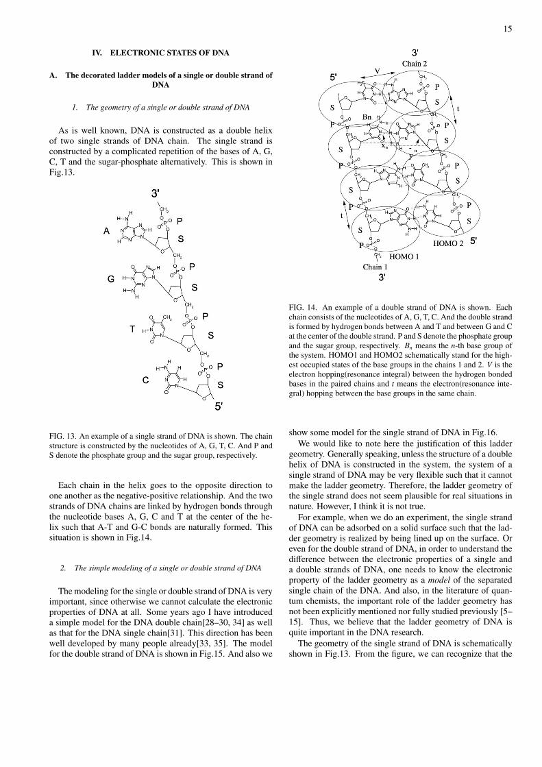
Each chain in the helix goes to the opposite direction toone another as the negative-positive relationship. And the twostrands of DNA chains are linked by hydrogen bonds throughthe nucleotide bases A, G, C and T at the center of the he-lix such that A-T and G-C bonds are naturally formed. Thissituation is shown in Fig.14.

2. The simple modeling of a single or double strand of DNA

The modeling for the single or double strand of DNA is veryimportant, since otherwise we cannot calculate the electronicproperties of DNA at all. Some years ago I have introduceda simple model for the DNA double chain[28–30, 34] as wellas that for the DNA single chain[31]. This direction has beenwell developed by many people already[33, 35]. The modelfor the double strand of DNA is shown in Fig.15. And also we

FIG. 14. An example of a double strand of DNA is shown. Eachchain consists of the nucleotides of A, G, T, C. And the double strandis formed by hydrogen bonds between A and T and between G and Cat the center of the double strand. P and S denote the phosphate groupand the sugar group, respectively. Bn means the n-th base group ofthe system. HOMO1 and HOMO2 schematically stand for the high-est occupied states of the base groups in the chains 1 and 2. V is theelectron hopping(resonance integral) between the hydrogen bondedbases in the paired chains and t means the electron(resonance inte-gral) hopping between the base groups in the same chain.

show some model for the single strand of DNA in Fig.16.We would like to note here the justification of this ladder

geometry. Generally speaking, unless the structure of a doublehelix of DNA is constructed in the system, the system of asingle strand of DNA may be very flexible such that it cannotmake the ladder geometry. Therefore, the ladder geometry ofthe single strand does not seem plausible for real situations innature. However, I think it is not true.

For example, when we do an experiment, the single strandof DNA can be adsorbed on a solid surface such that the lad-der geometry is realized by being lined up on the surface. Oreven for the double strand of DNA, in order to understand thedifference between the electronic properties of a single anda double strands of DNA, one needs to know the electronicproperty of the ladder geometry as a model of the separatedsingle chain of the DNA. And also, in the literature of quan-tum chemists, the important role of the ladder geometry hasnot been explicitly mentioned nor fully studied previously [5–15]. Thus, we believe that the ladder geometry of DNA isquite important in the DNA research.

The geometry of the single strand of DNA is schematicallyshown in Fig.13. From the figure, we can recognize that the

16

FIG. 15. The decorated ladder model of DNA – the simplest modelof a double strand of DNA is shown. (A) The schematic diagramof the DNA double chain. Here the repetition of the sugar(S) andphosphate(P) groups is emphasized. Hydrogen bonds are realizedbetween nucleotide A and nucleotide T or between nucleotide G andnucleotide C. (B) The decorated ladder model. It is the simplestmodeling for the double strand of DNA. Here the white(black) circlestands for the phosphate(sugar) site. The bonds between the chainstand for the hydrogen bonds. This is called the decorated laddermodel of DNA.

nucleotide base groups as big molecules are separated witheach other but the sugar-phosphate groups as small moleculesare linked with each other. This geometry allows electronsinevitably go through the backbone chain with an alternativerepetition of sugar-phosphate groups in the system.

On the other hand, we can also allow electrons hop be-tween the nucleotide base groups in the system. Here sincethe nucleotide base groups are lined up or twisted in the lad-der geometry, the overlap of the π-orbitals between the near-est nucleotide groups can be realized. Otherwise, this electronhopping must be difficult to occur in the system of the singlestrand of DNA.

Thus, we can understand that what is most important hereis the topology of electron hopping in the system such that theessential nature of the geometry of the single strand of DNAcan be regarded as a ladder.

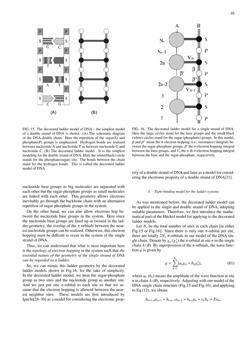
So, we can mimic this ladder geometry by the decoratedladder models shown in Fig.16, for the sake of simplicity.In the decorated ladder model, we treat the sugar-phosphategroup as two sites and the nucleotide group as another site.And we just put one π-orbital to each site so that we as-sume that the electron hopping is allowed between the near-est neighbor sites. These models are first introduced byIguchi[28–30] as a model for considering the electronic prop-

FIG. 16. The decorated ladder model for a single strand of DNA.Here the large circles stand for the base groups and the small black(white) circles stand for the sugar (phosphate) groups. In this model,β and β′′ mean the π-electron hopping (i.e., resonance) integrals be-tween the sugar-phosphate groups, β′ the π-electron hopping integralbetween the base groups, and Vn the n-th π-electron hopping integralbetween the base and the sugar-phosphate, respectively.

erty of a double strand of DNA and later as a model for consid-ering the electronic property of a double strand of DNA[31].

3. Tight-binding model for the ladder systems

As was mentioned before, the decorated ladder model canbe applied to the single and double strand of DNA, adoptingsuitable parameters. Therefore, we first introduce the mathe-matical part of the Huckel model for applying to the decoratedladder models.

Let Ns be the total number of sites in each chain [in eitherFig.15 or Fig.16]. Since there is only one π-orbital per site,there are totally 2Ns π-orbitals in our model of the DNA sin-gle chain. Denote by χn (χ′n) the π-orbital at site n in the singlechain A (B). By superposition of the π-orbitals, the wave func-tion φ is given by

φ =

Ns∑n=1

{anχn + bnχ′n}, (61)

where an (bn) means the amplitude of the wave function at siten in chain A (B), respectively. Adjusting with our model of theDNA single chain structure (Fig.15 and Fig.16), and applyingto Eq.(12), we obtain

hn+1,nan+1 + hn,n−1an−1 + hn,nan + vnbn = Ean,

17

h′n+1,nbn+1 + h′n,n−1bn−1 + h′n,nbn + v′nan = Ebn. (62)

Here hi j, h′i j are all the Huckel parameters of αii’s and βi j’sfor the system under investigation. And vn and v′n are theresonance integrals for the hydrogen bonds between the ad-jacent nucleotides. We would like to note that the conditionshn+1,n = h′n+1,n and vn = v′n are imposed without having anyproblem in the practical use. This reason has been explainedin the literature[28, 29].

4. Transfer matrix method

Let us find the transfer matrix method for Eq.(62). Definethe four-dimensional column vector, Ψn ≡ (an, an−1, bn, bn−1)t.Together with trivial relations, an = an and bn = bn, Eq.(62)can be converted into the following form:

Ψn+1 = MnΨn, (63)

Mn =

An Vn

Un Bn

, (64)

where Mn is the 4 × 4 transfer matrix with the 2 × 2 matrices:

An ≡ E−αn,n

βn+1,n− βn,n−1

βn+1,n

1 0

, Bn ≡ ε−α

′n,n

β′n+1,n− β

′n,n−1

β′n+1,n

1 0

, (65)

Un ≡ −vnβn+1,n

0

0 0

, Vn ≡ −v′nβ′n+1,n

0

0 0

. (66)

According to the sequence of Ns segments, we have to takea matrix product M of the Ns transfer matrices Mn such that

M(Ns) ≡ MNs MNs−1 · · ·M1, (67)

which is also a 4 × 4 matrix.We now impose that the single strand of DNA is periodic.

This means an+Ns = an and bn+Ns = bn, (i.e., Ψn+Ns = Ψn). Letus use this to Eq.(64). We then have Ψn+Ns = Ψn = M(Ns)Ψn.This provides the condition:

det[M(Ns) − I4] = 0, (68)

where I4 is the 4 × 4 unit matrix. Eq.(68) provides thewave vector k in the system such that k = 2π j/Ns for j =−Ns/2, · · · ,Ns/2.

Suppose next that the system is arbitrary large (i.e., Ns →∞) with the unit cell of N pairs of the nucleotide base and thesugar groups. Then we adopt the Bloch theorem to the system:

an+N = ρan, bn+N = ρbn (69)

with ρ = eikN . Applying Eq.(68) to Eq.(64), we find a 4 × 4determinant D(ρ) that is a fourth order polynomial of ρ:

D(ρ) ≡ det[M(N) − ρI4] =

ρ4 − s1ρ3 + s2ρ

2 − s3ρ + s4 = 0, (70)

where

M(N) ≡ MN MN−1 · · ·M1. (71)

By the relation between the roots and the coefficients the fourroots ρ1, ρ2, ρ3 and ρ4 are given by

s1 =

4∑i=1

ρi ≡ trM(N), s2 =

4∑i< j=1

ρiρ j,

s3 =

4∑i< j<k=1

ρiρ jρk, s4 = det M(N) ≡ ρ1ρ2ρ3ρ4. (72)

5. Symplectic property of the transfer matrix

Let us solve the biquadratic equation D(ρ) = 0. As wasproved previously[28–31], if ρ is a solution of the biquadraticequation, then so is ρ−1. Hence, ρ−1 must be an eigenvalue ofD(ρ) = 0 such that

D(ρ−1) = ρ−4(s4ρ4 − s3ρ

3 + s2ρ2 − s1ρ + 1) = 0. (73)

This gives us the particular property of the matrix M, calledthe symplectic structure[61],:

M†JM = J, (74)

J ≡ J 0

0 J

, J ≡ 0 −1

1 0

, (75)

where M† means the Hermitian conjugate of M and 0 is the2 × 2 zero matrix, respectively. This yields

D(ρ) = ρ4D(ρ−1), (76)

from which we find

s1 = s3, s4 = 1. (77)

Thus, M belongs to S L(4,R).By using this property and dividing D(ρ) by ρ2, the bi-

quadratic equation is reduced to the quadratic equation:

x2 − s1x + s2 − 2 = 0,

x = ρ +1ρ

(78)

Therefore, its two roots are given as

x± =12

(s1 ±

√D),

D = s21 − 4s2 + 8. (79)

18

As was shown in the literature[28, 29], by a simple manipula-tion using Eq.(72), we finally get

x± =12

[trM ±√

D],

D ≡ 2tr(M2) − (trM)2 + 8, (80)

where tr means the trace of matrix that is the sum of diagonalelements, and the − (+) channel means the bonding (antibond-ing) states between two parallel parts (i.e., the nucleotide basegroups and the sugar-phosphate groups) in the single strand ofDNA.

6. Scheme for obtaining the energy bands and the density of states

Now we can state a simple scheme to obtain the spectrumin the following: If an energy ε satisfies

x± = 2 cos kN, (81)

then the energy is allowed; otherwise it is forbidden in channel±, respectively. This can be regarded as a generalized versionof the Bloch condition for the single linear chain system withthe 2 × 2 transfer matrix M where

trM = 2 cos kN. (82)

We can also calculate the density of states (DOS) D±(ε) us-ing Eq.(80) together with Eq.(81) for each channel ±, respec-tively:

dk± =1N

d cos−1[x±(ε)/2]

= − 1N

∂x±∂ε√

4 − x2±

dε = D±(ε)dε. (83)

Therefore, the total DOS is given as the sum of D+(ε) andD−(ε):

D(ε) = D+(ε) + D−(ε), (84)

where D−(ε) [D+(ε)] means the DOS contributed from thebonding (antibonding) channel − (+), respectively.

B. The Electronic Properties of the single strand of DNA

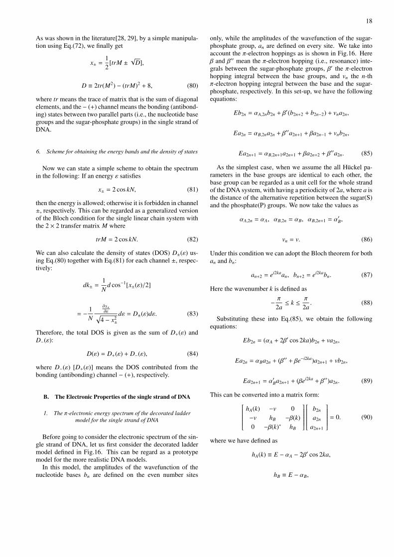
1. The π-electronic energy spectrum of the decorated laddermodel for the single strand of DNA

Before going to consider the electronic spectrum of the sin-gle strand of DNA, let us first consider the decorated laddermodel defined in Fig.16. This can be regard as a prototypemodel for the more realistic DNA models.

In this model, the amplitudes of the wavefunction of thenucleotide bases bn are defined on the even number sites

only, while the amplitudes of the wavefunction of the sugar-phosphate group, an are defined on every site. We take intoaccount the π-electron hoppings as is shown in Fig.16. Hereβ and β′′ mean the π-electron hopping (i.e., resonance) inte-grals between the sugar-phosphate groups, β′ the π-electronhopping integral between the base groups, and vn the n-thπ-electron hopping integral between the base and the sugar-phosphate, respectively. In this set-up, we have the followingequations:

Eb2n = αA,2nb2n + β′(b2n+2 + b2n−2) + vna2n,

Ea2n = αB,2na2n + β′′a2n+1 + βa2n−1 + vnb2n,

Ea2n+1 = αB,2n+1a2n+1 + βa2n+2 + β′′a2n. (85)

As the simplest case, when we assume the all Huckel pa-rameters in the base groups are identical to each other, thebase group can be regarded as a unit cell for the whole strandof the DNA system, with having a periodicity of 2a, where a isthe distance of the alternative repetition between the sugar(S)and the phosphate(P) groups. We now take the values as

αA,2n = αA, αB,2n = αB, αB,2n+1 = α′B,

vn = v. (86)

Under this condition we can adopt the Bloch theorem for bothan and bn:

an+2 = ei2kaan, bn+2 = ei2kabn. (87)

Here the wavenumber k is defined as

− π2a≤ k ≤ π

2a. (88)

Substituting these into Eq.(85), we obtain the followingequations:

Eb2n = (αA + 2β′ cos 2ka)b2n + va2n,

Ea2n = αBa2n + (β′′ + βe−i2ka)a2n+1 + vb2n,

Ea2n+1 = α′Ba2n+1 + (βei2ka + β′′)a2n. (89)

This can be converted into a matrix form:hA(k) −v 0−v hB −β(k)0 −β(k)∗ hB

b2n

a2n

a2n+1

= 0. (90)

where we have defined as

hA(k) ≡ E − αA − 2β′ cos 2ka,

hB ≡ E − αB,

19

β(k) ≡ −(β′′ + βe−i2ka),

h′B ≡ E − α′B. (91)

From this, we get the eigenvalue equation∣∣∣∣∣∣∣∣∣hA(k) −v 0−v hB −β(k)0 −β(k)∗ hB

∣∣∣∣∣∣∣∣∣ = 0. (92)

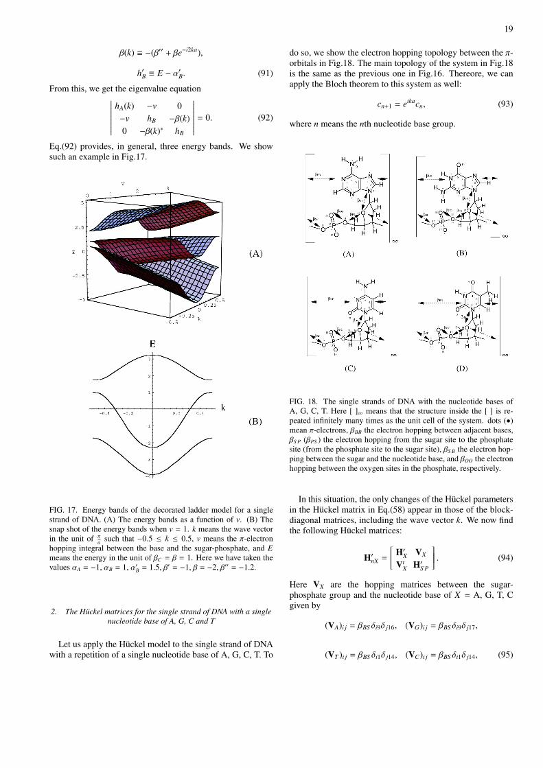
Eq.(92) provides, in general, three energy bands. We showsuch an example in Fig.17.

FIG. 17. Energy bands of the decorated ladder model for a singlestrand of DNA. (A) The energy bands as a function of v. (B) Thesnap shot of the energy bands when v = 1. k means the wave vectorin the unit of πa such that −0.5 ≤ k ≤ 0.5, v means the π-electronhopping integral between the base and the sugar-phosphate, and Emeans the energy in the unit of βC = β = 1. Here we have taken thevalues αA = −1, αB = 1, α′B = 1.5, β′ = −1, β = −2, β′′ = −1.2.

2. The Huckel matrices for the single strand of DNA with a singlenucleotide base of A, G, C and T

Let us apply the Huckel model to the single strand of DNAwith a repetition of a single nucleotide base of A, G, C, T. To

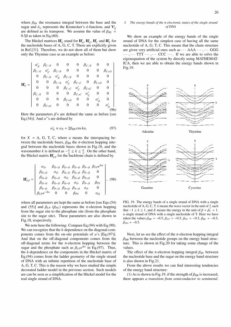
do so, we show the electron hopping topology between the π-orbitals in Fig.18. The main topology of the system in Fig.18is the same as the previous one in Fig.16. Thereore, we canapply the Bloch theorem to this system as well:

cn+1 = eikacn, (93)

where n means the nth nucleotide base group.

FIG. 18. The single strands of DNA with the nucleotide bases ofA, G, C, T. Here [ ]∞ means that the structure inside the [ ] is re-peated infinitely many times as the unit cell of the system. dots (•)mean π-electrons, βBB the electron hopping between adjacent bases,βS P (βPS ) the electron hopping from the sugar site to the phosphatesite (from the phosphate site to the sugar site), βS B the electron hop-ping between the sugar and the nucleotide base, and βOO the electronhopping between the oxygen sites in the phosphate, respectively.

In this situation, the only changes of the Huckel parametersin the Huckel matrix in Eq.(58) appear in those of the block-diagonal matrices, including the wave vector k. We now findthe following Huckel matrices:

H′nX =

H′X VX

VtX H′S P

. (94)

Here VX are the hopping matrices between the sugar-phosphate group and the nucleotide base of X = A, G, T, Cgiven by

(VA)i j = βBS δi9δ j16, (VG)i j = βBS δi9δ j17,

(VT )i j = βBS δi1δ j14, (VC)i j = βBS δi1δ j14, (95)

20

where βBS the resonance integral between the base and thesugar and δi j represents the Kronecker’s δ-function, and Vt

Xare defined as its transpose. We assume the value of βBS =

0.5β as taken in Eq.(60).The Huckel matrices H′X stand for H′A, H′G, H′C and H′T for

the nucleotide bases of A, G, C, T. These are explicitly givenin Ref.[31]. Therefore, we do not show all of them but showonly the Thymine case as an example as before:

H′T =

α′NβC−N 0 0 0 βC−N 0 0

βC−N α′CβC−N 0 0 0 0 βC=O

0 βC−N α′NβC−N 0 0 0 0

0 0 βC−N α′CβC−C 0 βC=O 0

0 0 0 βC−C α′CβC=C 0 0

βC−N 0 0 0 βC=C α′C

0 00 0 0 βC=O 0 0 α′

O0

0 βC=O 0 0 0 0 0 α′O

.

(96)Here the parameters β’s are defined the same as before [seeEq.(34)]. And α′’s are defined by

α′X ≡ αX + 2βBB cos ka, (97)

for X = A, G, T, C, where a means the interspacing be-tween the nucleotide bases, βBB the π-electron hopping inte-gral between the nucleotide bases shown in Fig.18, and thewavenumber k is defined as − πa ≤ k ≤ πa . On the other hand,the Huckel matrix H′S P for the backbone chain is defined by

H′S P =

αO βO−O βO−O βO−O βP−O βS Peika

βO−O αO βO−O βO−O βP−O 0βO−O βO−O αO βO−O βP=O 0βO−O βO−O βO−O αO βP−O βPS

βP−O βP−O βP=O βP−O αP 0βS Pe−ika 0 0 βPS 0 αO

, (98)

where all parameters are kept the same as before [see Eqs.(54)and (55)] and βS P (βPS ) represents the π-electron hoppingfrom the sugar site to the phosphate site (from the phosphatesite to the sugar site). These parameters are also shown inFig.18, respectively.

We note here the following: Compare Eq.(94) with Eq.(90).We can recognize that the k-dependence on the diagonal com-ponents comes from the on-site potentials of α’s [Eq.(97)].And that on the off-diagonal components comes from theoff-diagonal terms for the π-electron hopping between thesugar and the phosphate such as βS Peika in Eq.(97). Thus,the k-dependence on the components in the Huckel matrix ofEq.(94) comes from the ladder geometry of the single strandof DNA with an infinite repetition of the nucleotide base ofA, G, T, C. This is the reason why we have studied the simpledecorated ladder model in the previous section. Such modelsare can be seen as a simplification of the Huckel model for thereal single strand of DNA.

3. The energy bands of the π-electronic states of the single strandof DNA

We show an example of the energy bands of the singlestrand of DNA for the simplest case of having all the samenucleotide of A, G, T, C. This means that the chain structureare given very artificial ones such as · · · AAA · · · , · · · GGG· · · , · · · TTT · · · , · · · CCC · · · . If we are able to solve theeigenequation of the system by directly using MATHEMAT-ICA, then we are able to obtain the energy bands shown inFig.19.

FIG. 19. The energy bands of a single strand of DNA with a singlenucleotide of A, G, C, T. k means the wave vector in the unit of πa suchthat −1 ≤ k ≤ 1, and E means the energy in the unit of β = βC = 1.a single strand of DNA with a single nucleotide of T. Here we havetaken the values βBB = −0.5, βS P = −0.5, βPS = −0.5, βBS = −0.5,βOO = −0.5.

Next, let us see the effect of the π-electron hopping integralβBB between the nucleotide groups on the energy band struc-ture. This is shown in Fig.20 for taking some change of thevalues.

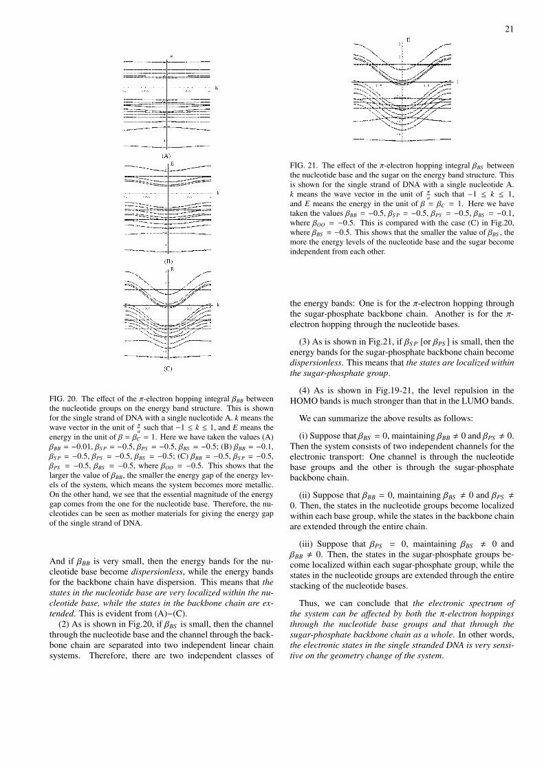
The effect of the π-electron hopping integral βBS betweenthe nucleotide base and the sugar on the energy band structureis also shown in Fig.21.

From the above results we can find interesting tendenciesof the energy band structure:

(1) As is shown in Fig.19, if the strength of βBB is increased,there appears a transition from semiconductor to semimetal.

21

FIG. 20. The effect of the π-electron hopping integral βBB betweenthe nucleotide groups on the energy band structure. This is shownfor the single strand of DNA with a single nucleotide A. k means thewave vector in the unit of πa such that −1 ≤ k ≤ 1, and E means theenergy in the unit of β = βC = 1. Here we have taken the values (A)βBB = −0.01, βS P = −0.5, βPS = −0.5, βBS = −0.5; (B) βBB = −0.1,βS P = −0.5, βPS = −0.5, βBS = −0.5; (C) βBB = −0.5, βS P = −0.5,βPS = −0.5, βBS = −0.5, where βOO = −0.5. This shows that thelarger the value of βBB, the smaller the energy gap of the energy lev-els of the system, which means the system becomes more metallic.On the other hand, we see that the essential magnitude of the energygap comes from the one for the nucleotide base. Therefore, the nu-cleotides can be seen as mother materials for giving the energy gapof the single strand of DNA.

And if βBB is very small, then the energy bands for the nu-cleotide base become dispersionless, while the energy bandsfor the backbone chain have dispersion. This means that thestates in the nucleotide base are very localized within the nu-cleotide base, while the states in the backbone chain are ex-tended. This is evident from (A)−(C).

(2) As is shown in Fig.20, if βBS is small, then the channelthrough the nucleotide base and the channel through the back-bone chain are separated into two independent linear chainsystems. Therefore, there are two independent classes of

FIG. 21. The effect of the π-electron hopping integral βBS betweenthe nucleotide base and the sugar on the energy band structure. Thisis shown for the single strand of DNA with a single nucleotide A.k means the wave vector in the unit of πa such that −1 ≤ k ≤ 1,and E means the energy in the unit of β = βC = 1. Here we havetaken the values βBB = −0.5, βS P = −0.5, βPS = −0.5, βBS = −0.1,where βOO = −0.5. This is compared with the case (C) in Fig.20,where βBS = −0.5. This shows that the smaller the value of βBS , themore the energy levels of the nucleotide base and the sugar becomeindependent from each other.

the energy bands: One is for the π-electron hopping throughthe sugar-phosphate backbone chain. Another is for the π-electron hopping through the nucleotide bases.

(3) As is shown in Fig.21, if βS P [or βPS ] is small, then theenergy bands for the sugar-phosphate backbone chain becomedispersionless. This means that the states are localized withinthe sugar-phosphate group.

(4) As is shown in Fig.19-21, the level repulsion in theHOMO bands is much stronger than that in the LUMO bands.

We can summarize the above results as follows:

(i) Suppose that βBS = 0, maintaining βBB , 0 and βPS , 0.Then the system consists of two independent channels for theelectronic transport: One channel is through the nucleotidebase groups and the other is through the sugar-phosphatebackbone chain.

(ii) Suppose that βBB = 0, maintaining βBS , 0 and βPS ,0. Then, the states in the nucleotide groups become localizedwithin each base group, while the states in the backbone chainare extended through the entire chain.

(iii) Suppose that βPS = 0, maintaining βBS , 0 andβBB , 0. Then, the states in the sugar-phosphate groups be-come localized within each sugar-phosphate group, while thestates in the nucleotide groups are extended through the entirestacking of the nucleotide bases.

Thus, we can conclude that the electronic spectrum ofthe system can be affected by both the π-electron hoppingsthrough the nucleotide base groups and that through thesugar-phosphate backbone chain as a whole. In other words,the electronic states in the single stranded DNA is very sensi-tive on the geometry change of the system.

22

C. The Electronic Properties of the double strand of DNA

1. The π-electronic energy spectrum of the decorated laddermodel for the double strand of DNA

Before going to consider the electronic spectrum of the dou-ble strand of DNA, we can use the same decorated decoratedladder model defined in Fig.15(as well as Fig.16) to this sys-tem as well. This can be regard as a prototype model for themore realistic models fore the double strand of DNA.

For our propose here, the equations that we need havebeen presented in §.X, by applying the Huckel method to thismodel. To use the equations, what we need is to assign theHuckel parameters for this model. We only consider the sim-plest case that all nucleotides are identical. In this case, wedefine the following:

βn+1,n = β′n+1,n = −β(= β′),

αn,n = α′n,n = 0,

vn = v′n = −v(= 0) at odd(even) n (99)

Applying this to Eq.(64), we have

M ≡ M1M2 =

E2

ββ′ −ββ′

Eβ

− vEββ′ 0

− Eβ− β

′

βvβ

0

− vEββ′ 0 E2

ββ′ −ββ′

Eβ

vβ

0 − Eβ− β

′

β

, (100)

Now we take the trM and trM2, and we obtain

12

trM =E2

ββ′−

(β

β′+β′

β

), (101)

12

trM2 =

E4

β2β′2−

[2(

1β2 +

1β′2

)− v2

β2β′2

]E2 +

β2

β′2+β′2

β2 , (102)

Substituting these into Eq.(80), we obtain

x± =E2

ββ′−

(β

β′+β′

β

)±

∣∣∣∣∣ vEββ′

∣∣∣∣∣ , (103)

where x± ≡ 2 cos 2k. Solving Eq.(103) for the energy E, weobtain the energy bands:

E(±)+ (k) =

12

(v ±

√v2 + 4

(β2 + β′2 + 2ββ′ cos 2k

)),

E(±)+ (k) =

12

(−v ±

√v2 + 4

(β2 + β′2 + 2ββ′ cos 2k

)), (104)

FIG. 22. Energy bands of the decorated ladder model for a doublestrand of DNA. (A) The energy bands as a function of v rangingv from 0 to 3. (B) The snap shot of the energy bands when v =0(thin curves) and v = 2(thick gray and black). Here v means the π-electron hopping integral between the base and the sugar-phosphate.The horizontal axis k means the wave vector in the unit of π/a suchthat −0.5 ≤ k ≤ 0.5, where a the interspacing between the basegroups. The verticai axis E means the energy in the unit of βC = β =1. The horizontal plane (i.e. EF = 0) means the position of the Fermienergy. We have taken the values α = 0, β = 1.2 and β′ = 0.9.

where E(+)± (k)[E(−)

± (k)] stand for the upper(lower) energybands in channels ±, respectively. These are shown in Fig.22.

We now observe that the spectrum is symmetric around E =0 and E(+)

± (k) > 0 > E(−)± (k) with respecr to k. The band gap at

the center of the spectrum is given by

∆0 = E(+)− (π/2) − E(−)

+ (π/2) =√

v2 + 4(β − β′)2 − v, (105)

and the overlapping of the two bands E(+)+ (k) and E(+)

− (k) isgiven by

∆1 = E(+)+ (π/2) − E(−)

− (0)

= v +12

[√v2 + 4(β − β′)2 −

√v2 + 4(β + β′)2

], (106)

23

Let us consider the above energy bands at half filling, EF =

0. In this model there is always a gap at E = 0 since As ∆0 > 0except the case of β = β′, contrary to the former case of theladder structure. However, there are several distinct charactersof the system classified in terms of ∆0 and ∆1.

(1) For v = 0, there are two doubly degenerate energybands separated by the gap ∆0 = 2|β− β′| with the band width∆1 = (β + β′ − |β − β′|)/2. So,the spectrum is semiconductor-like around E = 0. Hence, one expects that the system is asemiconductor at half filling.

(2) Suppose that

vc ≡2ββ′√β2 + β′2

. (107)

For 0 < v ≤ vc, the gap ∆0 persists to exist and the overlap-ping ∆1 is semimetal-like (i.e. ∆1 < 0) with the separationof v. Thus, the spectrum is again semiconductor-like at E :0.Hence, one expects that the system is a semiconductor at halffilling.

(3) For v > vc, another gap ∆1 appears so that ∆1 > 0 aswell as the gap ∆0 > 0. However, the spectrum is once againsemiconductor-like around E = 0. Hence, one expects thatthe system is a semiconductor at half filling.

In this way, if β − β′ , 0, then the system is maintained tobe a semiconductor for the whole range of v, in a strict sensethat there is always a gap at E = 0 in this model. However,unless v = 0, 1 find from Eq.(105) that if |(β−β′)/v| ≪ 1, then

∆0(v) ≈ 2|β − β′|2/v ≈ 0 ≪ ∆0(0) = 2|β − β′|. (108)

This tendency is enhanced as u is increased. Therefore, even ifthe center gap exists in the spectrum, it can be relatively smalland the system can behave like a metal at finite temperature inthe limit:

∆0 ≪ kBT < ∆0(0), (109)

where kB is the Boltzman constant and T the tempera-ture of the system. Thus, the system can show a kind ofsemiconductor-metal transition as v is increased. It is not anabsolute insulator-metal transition in the strict sense, but itmight be regarded as an effective one mediated at finite tem-perature.

2. The electronic conduction of the decorated ladder model for thedouble strand of DNA

Let us now consider the electronic property of DNA. Thiswas found long ago by Evans and Gergely[62] and found pe-culiar properties of DNA by Meade and Kayyem[63] about adecade ago. The former found that the electric conduction ofDNA follows the famous formula of semiconductor. The lat-ter found that the electronic conduction in the double strandof DNA is enhanced by the formation of the double strand ofDNA as large as 104 larger than that of the single strand ofDNA.

Let us now consider the electronic property of the π-electrons in the decorated ladder model for the double strand

of DNA[28, 29]. For this purpose, since we have the conduc-tion formula for the current I with the band gap ∆:

I = I0e−∆

kBT , (110)

where I0 is a constant, we just plague our expression of thecenter band gap into the energy gap ∆. This produces thecurrent Is when the double strand is broken to two separatechains such as

Is = I0e−∆0(0)kBT = I0e−

2|β−β′ |kBT . (111)

This is the case when v = 0. Similarly, when the double strandis formed such that v > 0, we obtain the conduction formulafor the current Id:

Id = I0e−∆0(v)kBT = I0e−

2|β−β′ |+√

v2+4|β−β′ |2 −vkBT (112)

In this way, we finally have the ratio Id/Is as

Id

Is∝ e−

∆0(v)kBT = I0e−

√v2+4|β−β′ |2 −v

kBT (113)

This was first obtained by the author[28, 29]. We show this re-sult in Fig.23. This result may explain such an intriguing prop-

FIG. 23. The relative current Id/Is. lt is shown for ∆0(0) = 2.4eV andkBT = 0.026eV . For the range of v ≈ 0.45− 0.64eV , it is the order ofthe magnitude of 104. The vertical axis means the relative current Id

in the unit of Is, while the horizontal axis means v.

erty of DNA conduction found by Meade and Kayyem[63].

3. The energy bands of the π-electronic states of the double strandof DNA

When we consider the π-electronic states of the doublestrand of DNA going beyond considering the π-electronicstates of the single strand of DNA, we may also use the sim-ilar method that has been introduced in §.XI. While a singlestrand of DNA is constructed such as

5′ − · · ·AAA · · · − 3′, 5′ − · · ·TTT · · · − 3′,

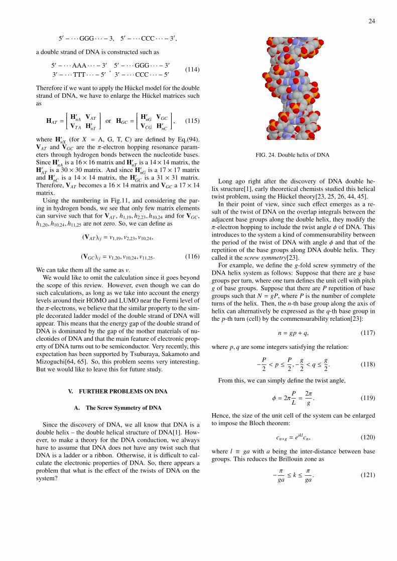
24

5′ − · · ·GGG · · · − 3, 5′ − · · ·CCC · · · − 3′,

a double strand of DNA is constructed such as

5′ − · · ·AAA · · · − 3′

3′ − · · ·TTT · · · − 5′,

5′ − · · ·GGG · · · − 3′

3′ − · · ·CCC · · · − 5′(114)

Therefore if we want to apply the Huckel model for the doublestrand of DNA, we have to enlarge the Huckel matrices suchas

HAT =

H′nA VAT

VT A H′nT

or HGC =

H′nG VGC

VCG H′nC

, (115)

where H′nX (for X = A, G, T, C) are defined by Eq.(94).VAT and VGC are the π-electron hopping resonance param-eters through hydrogen bonds between the nucleotide bases.Since H′nA is a 16× 16 matrix and H′nT is a 14× 14 matrix, theH′AT is a 30 × 30 matrix. And since H′nG is a 17 × 17 matrixand H′nC is a 14 × 14 matrix, the H′GC is a 31 × 31 matrix.Therefore, VAT becomes a 16 × 14 matrix and VGC a 17 × 14matrix.

Using the numbering in Fig.11, and considering the par-ing in hydrogen bonds, we see that only few matrix elementscan survive such that for VAT , h1,19, h2,23, h10,24 and for VGC ,h1,20, h10,24, h11,25 are not zero. So, we can define as

(VAT )i j = v1,19, v2,23, v10,24,

(VGC)i j = v1,20, v10,24, v11,25. (116)

We can take them all the same as v.We would like to omit the calculation since it goes beyond

the scope of this review. However, even though we can dosuch calculations, as long as we take into account the energylevels around their HOMO and LUMO near the Fermi level ofthe π-electrons, we believe that the similar property to the sim-ple decorated ladder model of the double strand of DNA willappear. This means that the energy gap of the double strand ofDNA is dominated by the gap of the mother materials of nu-cleotides of DNA and that the main feature of electronic prop-erty of DNA turns out to be semiconductor. Very recently, thisexpectation has been supported by Tsuburaya, Sakamoto andMizoguchi[64, 65]. So, this problem seems very interesting.But we would like to leave this for future study.

V. FURTHER PROBLEMS ON DNA

A. The Screw Symmetry of DNA

Since the discovery of DNA, we all know that DNA is adouble helix – the double helical structure of DNA[1]. How-ever, to make a theory for the DNA conduction, we alwayshave to assume that DNA does not have any twist such thatDNA is a ladder or a ribbon. Otherwise, it is difficult to cal-culate the electronic properties of DNA. So, there appears aproblem that what is the effect of the twists of DNA on thesystem?

FIG. 24. Double helix of DNA

Long ago right after the discovery of DNA double he-lix structure[1], early theoretical chemists studied this helicaltwist problem, using the Huckel theory[23, 25, 26, 44, 45].

In their point of view, since such effect emerges as a re-sult of the twist of DNA on the overlap integrals between theadjacent base groups along the double helix, they modify theπ-electron hopping to include the twist angle ϕ of DNA. Thisintroduces to the system a kind of commensurability betweenthe period of the twist of DNA with angle ϕ and that of therepetition of the base groups along DNA double helix. Theycalled it the screw symmetry[23].

For example, we define the g-fold screw symmetry of theDNA helix system as follows: Suppose that there are g basegroups per turn, where one turn defines the unit cell with pitchg of base groups. Suppose that there are P repetition of basegroups such that N = gP, where P is the number of completeturns of the helix. Then, the n-th base group along the axis ofhelix can alternatively be expressed as the q-th base group inthe p-th turn (cell) by the commensurability relation[23]:

n = gp + q, (117)

where p, q are some integers satisfying the relation:

−P2< p ≤ P

2,−g

2< q ≤ g

2. (118)

From this, we can simply define the twist angle,

ϕ = 2πPL=

2πg. (119)

Hence, the size of the unit cell of the system can be enlargedto impose the Bloch theorem:

cn+g = eiklcn, (120)

where l ≡ ga with a being the inter-distance between basegroups. This reduces the Brillouin zone as

− πga≤ k ≤ π

ga. (121)

25

And correspondingly, the energy bands E j(k) for the j-thmolecule can be given by

E j(k) = α j + 2β j cos(ka +

2πsg

), (122)

where s = 0, 1, · · · , g − 1[25, 26, 44, 45]. This result is notaffected by the change of the π-electron hopping parameters.Therefore, the energy bands degenerate at the zone boundarysuch that there are no band gaps between them[43].

To consider this effect, let us consider the π-electron hop-ping, βBi.B j ≡ βi j, between the i-th and j-th base groups. Wecan simply assume the approximation :

βi j = kS i j, (123)

where k is some constant and S i j the overlap integral of theπ-orbitals between the i-th and j-th base groups. If we areable to use this assumption, then the twist angle , ϕ, betweenthe base groups enters into the expression through the overlapintegral such as

S i j(ϕ) = S σσi j cos2 θ − S ππi j sin2 θ. (124)

Here S σσi j means the σ-bond like overlap integral and S ππi jmeans the π-bond like overlap integral of the π-orbitals of thei-th and j-th base groups. And θ is related to the twist angle ϕby

cos θ =

√a2 − (rϕ)2

a, (125)

where a is twice the interspacing between sugar-phosphategroup along the backbone of helix and r the distance from thecenter axis of helix to the position of the base group. Thiscan be derived from geometrical consideration[66]. FromEq.(123), we find

βi j(ϕ) = βσσi j cos2 θ − βππi j sin2 θ. (126)

Here βσσi j means the σ-bond like resonance integral and βππi jmeans the π-bond like resonance integral of the π-orbitals ofthe i-th and j-th base groups.

When the commensurability between the twist and thechange of the Huckel parameters is realized, there may ap-pear the band gaps at zone boundary. Therefore, the matchbetween the pitch of DNA and the overlapping of π-orbitalsis very crucial to have band gaps in the spectrum. However,at that time they assumed that the system is a linear objectof DNA like a line segment for the foundation of the theory.Therefore, in their theory even though they included the twistof the system, it was just like a torsion of the linear system.Hence, there appeared no much difference of the results fromthose of the standard linear chain system.

B. The effect of half-twist of DNA

We would like to discuss some peculiar mathematical prob-lem related to DNA, which seems very important for further

study. This is a problem when we think of the half-turns ofthe ladder or ribbon models. This has not been treated in theearly theoretical works in the above.

Consider the ladder structure of DNA in Fig.15. For ourprevious calculations, we always assumed the periodic bound-ary condition. This can be described as follows: Suppose thatboth ends of DNA are open ends with numbering 1 and Nsuch as in Fig.15. If we impose the periodicity to make anring geometry of DNA, then we have the periodicity of N forthe amplitudes of wave function as

an = an+N , bn = bn+N , (127)

or equivalently an+N

bn+N

= 1 00 1

an

bn

, (128)

where an are the amplitudes of wave function for helix A andbn that for helix B as in Eq.(62). This assures that when theunit cell of base group is simple enough we hold the Blochtheorem for the system such as

an+1 = eikaan, bn+1 = eikabn, (129)

where a stands for the spacing between nucleotide base groupsand −π/a ≤ k ≤ π/a with k j = 2π j/N for −N/2 ≤ j ≤ N/2.This means that there are totally 2N states for two channels,where for each channel there are N states[28, 29].

Let us now introduce a half-turn to the DNA ladder or DNAribbon to make a ring. Hence we encounter the problem oftopology of DNA[66] such that we have a Mobius strip ofDNA ladder or ribbon[67, 68]. In this case, Eq.(127) is nolonger correct. The boundary condition must be given by

an = bn+N , bn = an+N , (130)

or equivalently an+N

bn+N

= 0 11 0

an

bn

. (131)

Obviously, it is identical to the following:

cn = cn+2N , (132)

which means that there is no difference between an for chainA and bn for chain B for the system of the Mobius strip. Inother words, the double chain of length N in the ladder is en-larged to the single chain of length 2N so that the short rangeinteractions Vn,n ≡ vn through bridges between the neighborchains become the long distance interaction Vn,n+N betweensite n and site n + N in numbering.

Since we now have the Bloch theorem:

cn+1 = eikacn, (133)

we also have

cn+N = eikNacn, (134)

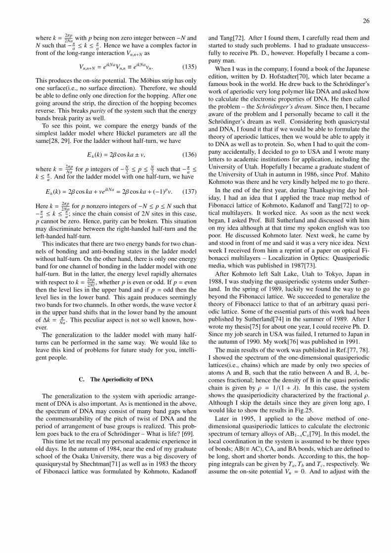
26

where k = 2πp2Na with p being non zero integer between −N and

N such that − πa ≤ k ≤ πa . Hence we have a complex factor infront of the long-range interaction Vn,n+N as

Vn,n+N = eikNaVn,n ≡ eikNavn. (135)

This produces the on-site potential. The Mobius strip has onlyone surface(i.e., no surface direction). Therefore, we shouldbe able to define only one direction for the hopping. After onegoing around the strip, the direction of the hopping becomesreverse. This breaks parity of the system such that the energybands break parity as well.

To see this point, we compare the energy bands of thesimplest ladder model where Huckel parameters are all thesame[28, 29]. For the ladder without half-turn, we have

E±(k) = 2β cos ka ± v, (136)

where k = 2πpNa for p integers of −N

2 ≤ p ≤ N2 such that − πa ≤

k ≤ πa . And for the ladder model with one half-turn, we have

E±(k) = 2β cos ka + veikNa = 2β cos ka + (−1)pv. (137)

Here k = 2πp2Na for p nonzero integers of −N ≤ p ≤ N such that

− πa ≤ k ≤ πa ; since the chain consist of 2N sites in this case,p cannot be zero. Hence, parity can be broken. This situationmay discriminate between the right-handed half-turn and theleft-handed half-turn.

This indicates that there are two energy bands for two chan-nels of bonding and anti-bonding states in the ladder modelwithout half-turn. On the other hand, there is only one energyband for one channel of bonding in the ladder model with onehalf-turn. But in the latter, the energy level rapidly alternateswith respect to k = 2πp

2Nl , whether p is even or odd. If p = eventhen the level lies in the upper band and if p = odd then thelevel lies in the lower band. This again produces seeminglytwo bands for two channels. In other words, the wave vector kin the upper band shifts that in the lower band by the amountof ∆k = π

Na . This peculiar aspect is not so well known, how-ever.

The generalization to the ladder model with many half-turns can be performed in the same way. We would like toleave this kind of problems for future study for you, intelli-gent people.

C. The Aperiodicity of DNA

The generalization to the system with aperiodic arrange-ment of DNA is also important. As is mentioned in the above,the spectrum of DNA may consist of many band gaps whenthe commensurability of the pitch of twist of DNA and theperiod of arrangement of base groups is realized. This prob-lem goes back to the era of Schrodinger – What is life? [69].

This time let me recall my personal academic experience inold days. In the autumn of 1984, near the end of my graduateschool of the Osaka University, there was a big discovery ofquasiqurystal by Shechtman[71] as well as in 1983 the theoryof Fibonacci lattice was formulated by Kohmoto, Kadanoff

and Tang[72]. After I found them, I carefully read them andstarted to study such problems. I had to graduate unsuccess-fully to receive Ph. D., however. Hopefully I became a com-pany man.

When I was in the company, I found a book of the Japaneseedition, written by D. Hofstadter[70], which later became afamous book in the world. He drew back to the Schrodinger’swork of aperiodic very long polymer like DNA and asked howto calculate the electronic properties of DNA. He then calledthe problem – the Schrodinger’s dream. Since then, I becameaware of the problem and I personally became to call it theSchrodinger’s dream as well. Considering both quasicrystaland DNA, I found it that if we would be able to formulate thetheory of aperiodic lattices, then we would be able to apply itto DNA as well as to protein. So, when I had to quit the com-pany accidentally, I decided to go to USA and I wrote manyletters to academic institutions for application, including theUniversity of Utah. Hopefully I became a graduate student ofthe University of Utah in autumn in 1986, since Prof. MahitoKohmoto was there and he very kindly helped me to go there.

In the end of the first year, during Thanksgiving day hol-iday, I had an idea that I applied the trace map method ofFibonacci lattice of Kohmoto, Kadanoff and Tang[72] to op-tical multilayers. It worked nice. As soon as the next weekbegan, I asked Prof. Bill Sutherland and discussed with himon my idea although at that time my spoken english was toopoor. He discussed Kohmoto later. Next week, he came byand stood in front of me and said it was a very nice idea. Nextweek I received from him a reprint of a paper on optical Fi-bonacci multilayers – Localization in Optics: Quasiperiodicmedia, which was published in 1987[73].

After Kohmoto left Salt Lake, Utah to Tokyo, Japan in1988, I was studying the quasiperiodic systems under Suther-land. In the spring of 1989, luckily we found the way to gobeyond the Fibonacci lattice. We succeeded to generalize thetheory of Fibonacci lattice to that of an arbitrary quasi peri-odic lattice. Some of the essential parts of this work had beenpublished by Sutherland[74] in the summer of 1989. After Iwrote my thesis[75] for about one year, I could receive Ph. D.Since my job search in USA was failed, I returned to Japan inthe autumn of 1990. My work[76] was published in 1991.

The main results of the work was published in Ref.[77, 78].I showed the spectrum of the one-dimensional quasiperiodiclattices(i.e., chains) which are made by only two species ofatoms A and B, such that the ratio between A and B, λ, be-comes fractional; hence the density of B in the quasi periodicchain is given by ρ = 1/(1 + λ). In this case, the systemshows the quasiperiodicity characterized by the fractional ρ.Although I skip the details since they are given long ago, Iwould like to show the results in Fig.25.

Later in 1995, I applied to the above method of one-dimensional quasiperiodic lattices to calculate the electronicspectrum of ternary alloys of AB1−xCx[79]. In this model, thelocal coordination in the system is assumed to be three typesof bonds; AB(≡AC), CA, and BA bonds, which are defined tobe long, short and shorter bonds. According to this, the hop-ping integrals can be given by Ta,Tb and Tc, respectively. Weassume the on-site potential Vn = 0. And to adjust with the

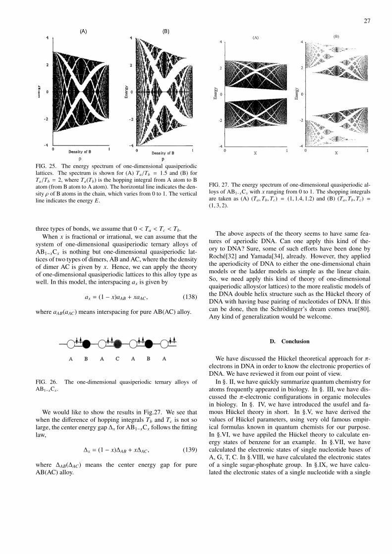
27

FIG. 25. The energy spectrum of one-dimensional quasiperiodiclattices. The spectrum is shown for (A) Ta/Tb = 1.5 and (B) forTa/Tb = 2, where Ta(Tb) is the hopping integral from A atom to Batom (from B atom to A atom). The horizontal line indicates the den-sity ρ of B atoms in the chain, which varies from 0 to 1. The verticalline indicates the energy E.

three types of bonds, we assume that 0 < Ta < Tc < Tb.When x is fractional or irrational, we can assume that the

system of one-dimensional quasiperiodic ternary alloys ofAB1−xCx is nothing but one-dimensional quasiperiodic lat-tices of two types of dimers, AB and AC, where the the densityof dimer AC is given by x. Hence, we can apply the theoryof one-dimensional quasiperiodic lattices to this alloy type aswell. In this model, the interspacing ax is given by

ax = (1 − x)aAB + xaAC , (138)

where aAB(aAC) means interspacing for pure AB(AC) alloy.

FIG. 26. The one-dimensional quasiperiodic ternary alloys ofAB1−xCx.

We would like to show the results in Fig.27. We see thatwhen the difference of hopping integrals Tb and Tc is not solarge, the center energy gap ∆x for AB1−xCx follows the fittinglaw,

∆x = (1 − x)∆AB + x∆AC , (139)

where ∆AB(∆AC) means the center energy gap for pureAB(AC) alloy.

FIG. 27. The energy spectrum of one-dimensional quasiperiodic al-loys of AB1−xCx with x ranging from 0 to 1. The shopping integralsare taken as (A) (Ta, Tb, Tc) = (1, 1.4, 1.2) and (B) (Ta,Tb, Tc) =(1, 3, 2).

The above aspects of the theory seems to have same fea-tures of aperiodic DNA. Can one apply this kind of the-ory to DNA? Sure, some of such efforts have been done byRoche[32] and Yamada[34], already. However, they appliedthe aperiodicity of DNA to either the one-dimensional chainmodels or the ladder models as simple as the linear chain.So, we need apply this kind of theory of one-dimensionalquaiperiodic alloys(or lattices) to the more realistic models ofthe DNA double helix structure such as the Huckel theory ofDNA with having base pairing of nucleotides of DNA. If thiscan be done, then the Schrodinger’s dream comes true[80].Any kind of generalization would be welcome.

D. Conclusion

We have discussed the Huckel theoretical approach for π-electrons in DNA in order to know the electronic properties ofDNA. We have reviewed it from our point of view.

In §. II, we have quickly summarize quantum chemistry foratoms frequently appeared in biology. In §. III, we have dis-cussed the π-electronic configurations in organic moleculesin biology. In §. IV, we have introduced the usufel and fa-mous Huckel theory in short. In §.V, we have derived thevalues of Huckel parameters, using very old famous empir-ical formulas known in quantum chemists for our purpose.In §.VI, we have appiled the Huckel theory to calculate en-ergy states of benzene for an example. In §.VII, we havecalculated the electronic states of single nucleotide bases ofA, G, T, C. In §.VIII, we have calculated the electronic statesof a single sugar-phosphate group. In §.IX, we have calcu-lated the electronic states of a single nucleotide with a single

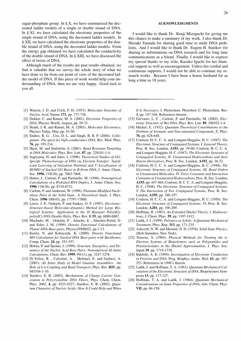
28

sugar-phosphate group. In §.X, we have summarized the dec-orated ladder models of a single or double strand of DNA.In §.XI, we have calculated the electronic properties of thesingle strand of DNA, using the decorated ladder models. In§.XII, we have calculated the electronic properties of the dou-ble strand of DNA, using the decorated ladder models. Fromthe energy gap obtained we have calculated the conductivityof the double strand of DNA. In §.XIII, we have discussed theeffect of twists of DNA.

Although much of the results are past results obtained, wefind it valuable that we survey the whole story of what wehave done so far from our point of view of the decorated lad-der model of DNA. If this piece of work would help your un-derstanding of DNA, then we are very happy. Good luck toyou all.

ACKNOWLEDGMENTS

I would like to thank Dr. Kenji Mizoguchi for giving methis chance to make a summary of my work. I also thank Dr.Hiroaki Yamada for sharing good time to study DNA prob-lems. And I would like to thank Dr. Eugeni B. Starikov forsharing us informations on DNA research and for long timecommunications as a friend. Finally, I would like to expressmy special thanks to my wife, Kazuko Iguchi for her finan-cial support as well as encouragement. Unless her cordial andcontinuous supports, I would not be able to continue my re-search works. Because I have been a house husband for aslong a time as 18 years.

[1] Watson, J. D. and Crick, F. H. (1953). Molecular Structure ofNucleic Acid, Nature 171, pp. 737-738.

[2] Dekker, C. and Ratner, M. A. (2001). Electronic Properties ofDNA, Physics World, August, pp. 29-33.

[3] Heath, J. R. and Ratner, M. A. (2003). Molecular Electronics,Physics Today, May, pp. 43-50.

[4] Endres, R. G. , Cox, D. L. and Singh, R. R. P. (2004). Collo-quium: The quest for high-conductance DNA, Rev. Mod. Phys.76, pp. 195-214.

[5] Hjort, M. and Stafstrom, S. (2001). Band Resonant Tunnelingin DNA Molecules, Phys. Rev. Lett. 87, pp. 228101-1-4.

[6] Sugiyama, H. and Saito, I. (1996). Theoretical Studies of GG-Specific Photocleavage of DNA via Electron Transfer: Signif-icant Lowering of Ionization Potential and 5’-Localization ofHOMO of Stacked GG Bases in B-Form DNA, J. Amer. Chem.Soc. 1996, 118(30), pp. 7063-7068.

[7] Hutter, J., Carloni, P. and Parrinello, M. (1996). NonempiricalCalculations of a Hydrated RNA Duplex, J. Amer. Chem. Soc.1996 118(38), pp. 8710-8712.

[8] Carloni, P. and Andreoni, W. (1996). Platinum-Modified Nucle-obase Pairs in the Solid State: A Theoretical Study, J. Phys.Chem. 1996 100(45), pp. 17797-17800.

[9] Lewis, J. P., Ordejon, P. and Sankey, O. F. (1997). Electronic-Structure-based Molecular-dynamics Method for Large Bio-logical Systems: Application to the 10 Basepair Poly(dG)-poly(dC) DNA Double Helix, Phys. Rev. B 55, pp. 6880-6887.

[10] Machado, M. , Ordejon, P. , Artacho, E. , Sanchez-Portal, D.and Soler, J. M. (1999). Density Functional Calculations ofPlanar DNA Base-pairs, Physics/9908022, pp.1-12.

[11] Kurita, N. and Kobayashi, K. (2000). Density FunctionalMO Calculation for Stacked DNA Base-pairs with Backbones,Comp. Chem. 24, pp. 351-357.

[12] Hobza, P. and Sponer, J. (1999). Structure, Energetics, and Dy-namics of the Nucleic Acid Base Pairs: Nonempirical Ab InitioCalculations, Chem. Rev. 1999, 99(11), pp. 3247-3276.

[13] Di Felice, R. , Calzolari, A. , Molinari, E. and Garbesi, A.(2001). Ab Initio Study of Model Guanine Assemblies: theRole of π-π Coupling and Band Transport, Phys. Rev. B55, pp.045104-1-10.

[14] Starikov. E. B. (2002). Mechanisms of Charge Carrier Gen-eration in Polycrystalline DNA Fibers, Phys. Chem. Chem.Phys. 2002, 4, pp. 4523-4527; Starikov. E. B. (2002). Quan-tum Chemistry of Nucleic Acids: How It Could Help and When

It Is Necessary, J. Photochem. Photobiol. C: Photochem. Rev.3, pp. 147-164. References therein.

[15] Gervasio, L. F. , Carloni, P. and Parrinello, M. (2002). Elec-tronic Structure of Wet DNA, Phys. Rev. Lett. 89, 108102-1-4.

[16] Huckel, E. (1932). Quantum Theoretical Contributions to theProblem of Aromatic and Non-saturated Compounds, Z. Phys.76, pp. 628-648.

[17] Coulson, H. C. C. A. and Longuet-Huggins, H. C. (1947). TheElectronic Structure of Conjugated Systems. I. General Theory,Proc. R. Soc. London, A191, pp. 39-60; Coulson, H. C. C. A.and Longuet-Huggins, H. C. (1947). The Electronic Structure ofConjugated Systems. II. Unsaturated Hydrocarbons and theirHetero-Derivatives, Proc. R. Soc. London, A192, pp. 16-32.

[18] Coulson, H. C. C. A. and Longuet-Huggins, H. C. (1948). TheElectronic Structure of Conjugated Systems. III. Bond Ordersin Unsaturated Molecules; IV. Force Constants and InteractionConstants in Unsaturated Hydrocarbons, Proc. R. Soc. London,A193, pp. 447-464; Coulson, H. C. C. A. and Longuet-Huggins,H. C. (1948). The Electronic Structure of Conjugated Systems.V. The Interaction of Two Conjugated Systems, Proc. R. Soc.London, A195, pp. 188-197.

[19] Coulson, H. C. C. A. and Longuet-Huggins, H. C. (1950). TheElectronic Structure of Conjugated Systems. VI, Proc. R. Soc.London, A201, pp. 196-209.

[20] Hoffman, R. (1963). An Extended Huckel Theory. I. Hydrocar-bons, J. Chem. Phys. 39, pp. 1397-1412.

[21] Ladik, J. J. (1999). Polymers as Solids: A Quantum MechanicalTreatment, Phys. Rep. 313, pp. 171-235.

[22] Ashcroft, N. W. and Mermin, N. D. (1976). Solid State Physics,(Holt-Saunders, New York).

[23] Yomosa, S. (1964). Physical Methods for Treating the π-Electron Systems of Biopolymers such as Polypeptides andPolynucleotides in the Huckel Approximation, J. Phys. Soc.Japan 19, pp. 1718-1730.

[24] Bakhshi, A. K. (1994). Investigation of Electronic Conductionin Proteins and DNA, Prog. Biophys. molec. Biol. 61, pp. 187-253. References in 1990’s therein.

[25] Ladik, J. and Hoffman, T. A. (1963). Quantum Mechanical Cal-culation of the Electronic Structure of DNA, Biopolymers Sym-posia 13, pp. 117-127.

[26] Hoffman, T. A. and Ladik, J. (1964). Quantum MechanicalConsiderations on Some Properties of DNA, Adv. Chem. Phys.VII, pp. 84-158;

29

[27] Ladik, J. and Biczo, G. (1965). Energy-Band Calculations forPeriodic DNA Models in the Huckel Approximation, J. Chem.Phys. 42, pp. 1658-1662. References in 1960’s therein. This isabout the time of birth of quantum chemistry.

[28] Iguchi, K. (1997). Tight-binding Model for DNA DoubleChains: Metal-insulator Transition Due to the Formation of aDouble Strand of DNA, Int. J. Mod. Phys. 11, pp. 2405-2423.

[29] Iguchi, K. (2001). Semiconductivity and Band Gap of a DoubleStrand of DNA, J. Phys. Soc. Japan 70, pp. 593-597.

[30] Iguchi, K. (2003). Extrinsic Semiconductor Character of aDouble Strand of DNA: Holstein’s Polarons as Donors and Ac-ceptors, Int. J. Mod. Phys. 17, pp. 2565-2578.

[31] Iguchi, K. (2004). π-Electrons in a Single Strand of DNA: APhenomenological Approach, Int. J. Mod. Phys. 13, pp. 1845-1910.

[32] Roche, S. (2003). Sequence Dependent DNA-mediated Conduc-tion, Phys. Rev. Lett. 91, pp. 108101-1-4; Roche, S., Bicout,D., Macia, E., and Kats, E. (2003). Long Range Correlations inDNA: Scaling Properties and Charge Transfer Efficiency, Phys.Rev. Lett. 91, 228101-1-4.

[33] Macia Barber, E. (2008). Aperiodic Structures in CondensedMatter: Fundamentals and Applications, (Taylor & Francis,New York). References therein.

[34] Yamada, H. (2004). Electronic Localization Properties of aDouble Strand of DNA: A Simple Model with Long-range Cor-related Hopping Disorder, Int. J. Mod. Phys. B18, pp. 1697-1716; Yamada, H. (2004). Localization of Electronic States inChain Models Based on Real DNA Sequence, Phys. Lett. A 332,pp. 65-73.

[35] Yamada, H. and Iguchi, K. (2010). Some Effective Tight-Binding Models for Electrons in DNA Conduction: A Review,Adv. in Cond. Mat. Phys. 2010, 380710.

[36] Klotsa, D., Romer, R. A. and Turner, M. S. , (2005). ElectronicTransport in DNA, Biophys. J. 89, pp. 2187-2198.

[37] Wang, H. , Marsh, R. , Lewis, J. P. and Romer, R. A. (2006).Electronic transport and localization in short and long DNA,in Modern Methods for Theoretical Physical Chemistry ofBiopolymers, edited by E. B. Starikov, J. P. Lewis, S. Tanaka,(Elsevier B. V., Amsterdam), Chap 21, pp.407-428.

[38] Cuniberti, G. , Macia, E. , Rodrıguez, A. and Romer, R. A.(2007). Tight-Binding Modeling of Charge Migration in DNADevices, in Charge Migration in DNA, edited by Prof. Dr. T.Chakraborty, (Springer Berlin Heidelberg) pp.1–20.

[39] Fukui, K. (1976). Chemical Reactions and Electronic Orbitals,(Maruzen, Tokyo), in Japanese.

[40] Burdett, J. K. (1984). From Bonds to Bands and Molecules toSolids, Prog. Solid St. Chem. 15, pp. 173-255.

[41] Nagata, Chikayoshi (2002). private communications throughpostal mails (Jan. 25). He was one of graduate students fromKen-Ichi Fukui who got Nobel prize for the discovery of fron-tier electrons.

[42] Stryer, L. (1988). Biochemistry, Third Ed., (Freeman and Com-pany, New York).

[43] Yomosa, S. (1965). Electronic Structures of Proteins, in Quan-tum Chemistry II, Lecture Series in Biophysics, (YoshiokaShoten, Kyoto), pp. 3-74(in Japanese).

[44] Nagata, C. (1965). Electronic Structures of DNA, in QuantumChemistry II, Lecture Series in Biophysics, (Yoshioka Shoten,Kyoto), pp. 75-112(in Japanese).

[45] Nagata, C. (1975). Introduction to Quantum Biology, (GakkaiShuppan Center, Tokyo), in Japanese.

[46] Pullman, B. and Pullman, A. (1960). Some Electronic Aspectsof Biochemistry, Rev. Mod. Phys. 32, pp. 428-436.

[47] Chiang, C. K. , Fincher, Jr., C. R. , Park, Y. W., Heeger, A. J. ,

Shirakawa, H., Louis, E. J., Gau, S. C. and MacDiarmid, A. G.(1977). Electrical Conductivity in Doped Polyacetylene, Phys.Rev. Lett. 39, pp. 1098-1101.

[48] Heeger, A. J. , Kivelson, S., Schrieffer, J. R., and Su, W.-P.(1988). Solitons in Conducting Polymers, Rev. Mod. Phys. 60,pp. 781-850.

[49] Fukui, K., Morokuma, K., and Nagata, C. (1960). A MolecularOrbital Treatment of Phosphate Bonds of Biochemical Interest.I. Simple LCAO MO Treatment, Bull. Chem. Soc. Japan 33, pp.1214-1219.

[50] Fukui, K., Imamura, A. and Nagata, C. (1963). A MolecularOrbital Treatment of Phosphate Bonds of Biochemical Interest.II. Metal Chelates of Adenosine Triphosphate, Bull. Chem. Soc.Japan 33, pp. 1450-1453.

[51] Boyd, D. B. and Lipscomb, W. N. (1969). Electronic Structuresfor Energy-rich Phosphates, J. Theor. Biol. 25, pp. 403-420.

[52] Mulliken, R. S. (1955). Electronic Population Analysis onLCAO-MO Molecular Wave Functions. II. Overlap Popula-tions, Bond Orders, and Covalent Bond Energies, J. Chem.Phys. 23, pp. 1841-1846.

[53] Wolfsberg, M. and Helmholtz, L. (1952). The Spectra and Elec-tronic Structure of the Tetrahedral Ions MnO−4 , CrO−−4 , andClO−4 , J. Chem. Phys. 20, pp. 837-843.

[54] Sandorfy, C. (1949). Etude Sur Le Role Des Substitutants EtDes Heteroatomes Dans Le Noyau Benzenique, Bull. Soci.Chim. de France, 16, pp. 615-626.

[55] Streiwieser, Jr., A. (1961). Molecular Orbital Theory for Or-ganic Chemists, (John Willey & Sons, Inc., New York), Chap.5.

[56] Mulliken, R. S., Rieke, C. A., Orloff, D. and Orloff, H.(1949). Formulas And Numerical Tables For Overlap Integrals,J. Chem. Phys. 17, pp. 1248-1267.

[57] C. J. Ballhausen and H. B. Gray. (1964). Molecular OrbitalTheory, (Benjamin, Ne York), p.158.

[58] Prichard, H. O. and Skinner, H. A. (1955). The Concept of Elec-tronegativity, Chem. Rev. 1955, 55(4), pp. 745-786.

[59] Vela, A. and Gazquez, J. L. (1988). Extended Huckel Param-eters from Density Functional Theory, J. Phys. Chem. 92, pp.5688-5693.

[60] Zhao, J. and Lu, J. P. (2003). A Nonorthogonal Tight-bindingTotal Energy Model for Molecular Simulations, Phys. Lett. A319, pp. 523-529.

[61] Arnold, V. I. (1989). Mathematical Methods of Classical Me-chanics, Second Edition, (Springer-Verlag, Berlin), p.225.

[62] Eley, D. D. and Spivey, D. I. (1962). Semiconductivity ofOrganic Substances. Part 9.―Nucleic Acid in the Dry State,Trans. Faraday Soc. 58, pp. 411-415.

[63] T. J. Meade and J. F. Kayyem. (1995). Angew. Chem. Int. Ed.Engl. 34, 352.

[64] Mizoguchi, K., Tanaka, S., Ogawa, T., Shiobara, N. andSakamoto, H. (2005). Magnetic Study of the Electronic Statesof B-DNA and M-DNA Doped with Metal Ions, Phys. Rev B 72,0233106-1-4.

[65] Tsuburaya, M. , Sakamoto, H. and Mizoguchi, K. (2014). Elec-tronic States of DNA and M-DNA Studied by Optical Absorp-tion, Phys. Rev E 89, 022719-1-7.

[66] White, J. H. and Bauer, W. R. (1986). Calculation of the Twistand the Writhe for Representative Models of DNA, J. Mol. Biol.189, pp. 329-341.

[67] Mila, F., Stafford, C. A. and Capponi, S. (1998). Persistent Cur-rents in a Mobius Ladder: A Test of Interchain Coherence ofInteracting Electrons, Phys. Rev B 57, pp. 1457-1460.

[68] Hayashi, M. and Ebisawa, H. (2001). Little-Parks Oscillation ofSuperconducting Mobius Strip, J. Phys. Soc. Japan 70, pp.3495-3498.

30

[69] Schrodinger, E. (1967). What is life? & Mind and Matter,(Cambridge University, Cambridge, 1967).

[70] Hofstadter, D. R. (1979). Godel, Esher, Bach: An EternalGolden Braid, (Vintage Books, New York); translated intoJapanese (Hakuyosha, Tokyo, 1985).

[71] Shechtman, D., Blech, I., Gratias, D., and Cahn, J. W. (1984).Metallic Phase with Long-range Orientational Order and NoTranslational Symmetry, Phys. Rev. Let., 53, pp. 1951-1953.

[72] Kohmoto, M., Kadanoff, L. P., and Tang, C. (1983). Localiza-tion Problem in One Dimension: Mapping and Escape, Phys.Rev. Let., 50, pp. 1870-1872.

[73] Kohmoto, M., Sutherland, B., and Iguchi, K. (1987). Localiza-tion of Optics: Quasiperiodic Media, Phys. Rev. Lett., 58, pp.2436-2438.

[74] Sutherland, B. (1989). Quasiperiodic Physics in One Dimen-sion, in Disorder and Nonlinearity, edited byA. B. Bishop,D. K. Campbell, and S. Pnevmatikos, (Springer-Verlag, NewYork), pp. 62-69.

[75] Iguchi, K. (1990). Theory of Quasiperiodic Lattices, Ph. D.

Thesis, Deprt. of Phys., The University of Utah, Salt Lake City,Utah, USA.

[76] Iguchi, K. (1991). Theory of Quasiperiodic Lattices. I. ScalingTransformation for a Quasiperiodic Lattice, Phys. Rev. B, 43,pp. 5915-5918; Theory of Quasiperiodic Lattices. II. GenericTrace Map and Invariant Surface, Phys. Rev. B, 43, pp. 5919-5923.

[77] Iguchi, K. (1992). Exact Wave Functions of An Electron onA Quasiperiodic Lattice: Definition of An Infinite-dimensionalRiemann Theta Function, J. Math. Phys. 33, pp. 3938-3947.

[78] Iguchi, K. (1994). Some Remarks on the Theory of An Electronon Binary Quasiperiodic Lattices, Int. J. Mod. Phys. B 8, pp.1931-1964.

[79] Iguchi, K. (1995). Electronic Structure of One-DimensionalQuasiperiodic Materials of AB1−xCx, J. Phys. Soc. Japan, 64,pp. 177-184.

[80] Iguchi, K. (1994). The Schrodinger’s Dream: Electronic Struc-ture of DNAs and Proteins: Quantum Automata, RIKEN Re-view 6, pp. 49-50.